NBER WORKING PAPER SERIES

SUBWAYS, STRIKES, AND SLOWDOWNS:THE IMPACTS OF PUBLIC TRANSIT ON TRAFFIC CONGESTION

Michael L. Anderson

Working Paper 18757http://www.nber.org/papers/w18757

NATIONAL BUREAU OF ECONOMIC RESEARCH1050 Massachusetts Avenue

Cambridge, MA 02138February 2013

I thank Ken Small, Lowell Taylor, Matt Turner, and participants at the 13th Occasional CaliforniaWorkshop on Environmental and Resource Economics, the 2012 AERE Summer Conference, TexasA&M, and the University of Houston for valuable suggestions. Any errors in the paper are the author’s.The views expressed herein are those of the author and do not necessarily reflect the views of the NationalBureau of Economic Research.

NBER working papers are circulated for discussion and comment purposes. They have not been peer-reviewed or been subject to the review by the NBER Board of Directors that accompanies officialNBER publications.

© 2013 by Michael L. Anderson. All rights reserved. Short sections of text, not to exceed two paragraphs,may be quoted without explicit permission provided that full credit, including © notice, is given tothe source.

Subways, Strikes, and Slowdowns: The Impacts of Public Transit on Traffic CongestionMichael L. AndersonNBER Working Paper No. 18757February 2013JEL No. R41,R42,R48

ABSTRACT

Public transit accounts for only 1% of U.S. passenger miles traveled but nevertheless attracts strongpublic support. Using a simple choice model, we predict that transit riders are likely to be individualswho commute along routes with the most severe roadway delays. These individuals’ choices thus havevery high marginal impacts on congestion. We test this prediction with data from a sudden strike in2003 by Los Angeles transit workers. Estimating a regression discontinuity design, we find that averagehighway delay increases 47% when transit service ceases. This effect is consistent with our model’spredictions and many times larger than earlier estimates, which have generally concluded that publictransit provides minimal congestion relief. We find that the net benefits of transit systems appear tobe much larger than previously believed.

Michael L. AndersonDepartment of Agricultural and Resource Economics207 Giannini Hall, MC 3310University of California, BerkeleyBerkeley, CA 94720and NBERmlanderson@berkeley.edu

! 1

1. INTRODUCTION

It is a stylized fact in the transportation literature that mass transit attracts a

disproportionate share of public funds but carries a negligible fraction of commuters. In

2010, public transit received 23% of federal highway and transit outlays but accounted for

1% of passenger miles traveled (U.S. Department of Transportation 2009, 2011a, 2011b).

State, local, and federal subsidies exceed $40 billion per year and cover 63% of operating

costs and 100% of capital costs. Even in Washington, DC – which boasts the second busiest

metro system in the United States – transit accounts for only 5% of passenger miles traveled

(American Public Transportation Association 2011; Schrank, Lomax, and Eisele 2011).

Public transit subsidies nevertheless remain popular in many areas. For example, in 2008

67% of Los Angeles County residents voted to allocate $26 billion to transit over 30 years.

Why is there such deep public support for transit subsidies if few voters are frequent riders?

The simplest explanation is the possibility of congestion relief – commuters may expect to

benefit from reduced congestion even if they rarely use public transit themselves.1 A large

body of transportation and economic research, however, concludes that public transit has

little effect on reducing congestion, calling into question its heavy subsidy rate (Rubin,

Moore, and Lee 1999; Stopher 2004; Small 2005; Winston and Maheshri 2007).

An important detail that has received little attention in the existing literature is that

commuters on different roadways in the same metropolitan area face sharply different levels

of congestion during peak hours. This paper presents a simple choice model in which

commuters face differing levels of congestion and choose either to drive or take transit.

Calibrating the model using data from the Los Angeles metro area, we predict effects on

congestion that are approximately six times larger than a model that does not account for

heterogeneity in congestion levels. This prediction is much larger than previous estimates,

and the qualitative conclusion is robust to wide variations in parameter values. The intuition

is straightforward: Transit is most attractive to commuters who face the worst congestion, so

a disproportionate number of transit riders are commuters who would otherwise have to

drive on the most congested roads at the most congested times. Since drivers on heavily

congested roads have a much higher marginal impact on congestion than drivers on the

average road, transit has a large impact on reducing traffic congestion.

!!!!!!!!!!!!!!!!!!!!!!!!!!!!!!!!!!!!!!!!!!!!!!!!!!!!!!!!1 This possibility is perhaps best summarized by the title of a satirical article in the November 29, 2000, issue of The Onion, “Report: 98 Percent of U.S. Commuters Favor Public Transportation for Others.” Other factors that may explain local support of capital investment in transit include high federal matching rates, a combination of concentrated economic rents and dispersed costs, and the political appeal of “ribbon cutting” ceremonies (Taylor 2004; Baum-Snow and Kahn 2005; Winston and Maheshri 2007).

! 2

We test our predictions using freeway speed data from a 2003 strike by Los Angeles

County Metropolitan Transportation Authority (MTA) workers. In October 2003, MTA

workers began a strike that lasted 35 days and shut down MTA bus and rail lines. Using

hourly data on traffic speeds for all major Los Angeles freeways, we estimate a regression

discontinuity (RD) design using time as the running variable. We find an abrupt increase in

average delays of 47% (0.19 minutes per mile) during peak periods. This increase persists

through the end of the strike, and the estimate – consistent with the predictions of our

model – is many times larger than estimates in the existing literature. The effects are largest

on freeways that parallel transit lines with heavy ridership, and they are small and statistically

insignificant during the same period in neighboring counties unaffected by the transit strike.

Our estimates imply that the total congestion relief benefit of operating the Los Angeles

transit system is between $1.2 billion to $4.1 billion per year, or $1.20 to $4.10 per peak-hour

transit passenger mile. We consider the potential gap between the short-run effect of ceasing

transit provision (i.e., our estimates) and the long-run effect of a permanent shutdown. We

find that reducing the long-run effect to less than 50% of the short-run effect’s lower bound

requires implausibly large elasticities of travel with respect to travel costs. We consider the

net benefits of constructing the Los Angeles rail system and conclude – contrary to the

existing literature on rail capital investment – that they are large and positive.

On a broader scale, our findings demonstrate that in contexts in which policymakers

encourage adoption of activities that mitigate negative externalities, considering who adopts

the mitigating activity is critical in determining a policy’s expected benefits. We close with a

brief discussion of other contexts in which selection into mitigating activities may have large

impacts on predicted benefits.

2. BACKGROUND

Existing economic research on the effects of transit on traffic congestion falls into two

categories: model-based estimates and empirical estimates. Examples of the former include

Nelson et al. (2007) and Parry and Small (2009). Parry and Small (2009) develop an analytical

model of an urban transportation system and compute the optimal transit operating subsidy.

The model takes as inputs average speeds, costs, and price and service elasticities. One input

is the effect of transit on relieving traffic congestion. They compute this effect using

assumptions about substitution between transportation modes and engineering estimates

relating average delays and marginal congestion impacts. In Los Angeles, the congestion

relief externality of traveling 1 mile on transit during peak hours is computed at 1.7 person-

! 3

minutes of reduced traffic delays.2 Aggregating this figure across all peak-period transit

passengers implies that transit reduces average delay by approximately 5% (0.025 minutes

per mile). Nelson et al. explore the potential benefits of the Washington, DC transit system

using a simulation model in which travel decisions are modeled as a nested logit tree. The

model takes as inputs demand response parameters from the literature, and it is calibrated to

match aggregate Washington travel patterns. Applying a relationship between traffic flows

and traffic speeds similar to that used by Parry and Small, Nelson et al. calculate that the

Washington transit system reduces total congestion by 184,000 person-hours per day, or 2.0

person-minutes per peak transit passenger mile carried. This figure is close to the figure

implied by Parry and Small.

Researchers employing empirical approaches include Winston and Langer (2006) and

Duranton and Turner (2011). Using metropolitan-area data, these authors regress total

congestion or vehicle miles traveled (VMT) on measures of transit capacity. They reach

varying conclusions. Winston and Langer estimate that rail lines reduce congestion but that

bus lines increase congestion. The net effect of transit systems is thus to increase congestion.

Duranton and Turner focus on testing the “fundamental law of road congestion” – the

hypothesis that the primary determinant of VMT in most cities is roadway capacity. They

also estimate a positive relationship between bus fleet size and VMT. To address the

potential endogeneity of transit provision, they instrument for bus fleets using an area’s 1972

Democratic vote share. The relationship between bus fleets and VMT then becomes

statistically insignificant and of variable sign, though the instrument is not powerful enough

to rule out the possibility that 1 passenger mile traveled on transit removes substantially

more than 1 VMT from roadways.3 These findings are nevertheless consistent with our own

findings, which suggest that transit has a minimal impact on total VMT but a large impact on

!!!!!!!!!!!!!!!!!!!!!!!!!!!!!!!!!!!!!!!!!!!!!!!!!!!!!!!!2 In Los Angeles, Parry and Small assume that each passenger mile traveled on transit diverts approximately 0.9 passenger miles from roadways. The average peak period delay in Los Angeles is 0.5 minutes per mile, and estimates from the literature relating traffic flows and traffic speeds suggest that the marginal effect on total delay of adding an additional vehicle to the road is 3.7 times the average delay. The congestion relief externality of traveling 1 mile on transit during peak hours is thus (–0.9 auto passenger miles/transit passenger mile * 0.5 mins avg delay/passenger mile * 3.7 mins increased delay/min avg delay) = –1.7 mins increased delay/transit passenger mile. 3 Duranton and Turner estimate that increasing a city’s bus fleet by 18 buses (10%) changes annual VMT by –1.3% to 0.6% (–35 million to 16 million VMT) in their most precise instrumental variables (IV) specification and –0.7% to 4.9% (–18 million to 133 million VMT) in their least precise IV specification (these figures correspond to 95% confidence intervals). An average city bus carries 0.3 million passenger miles per year (American Public Transit Association 2011), so adding 5.4 million passenger miles of bus travel could decrease VMT by up to 35 million miles in the most precise specification and up to 18 million miles in the least precise specification.

! 4

congestion levels. As we demonstrate below, the type of VMT diverted to transit is critical in

determining transit’s effects on congestion.

Overall, existing economic research does not support the hypothesis that transit

generates large aggregate reductions in traffic congestion. Though transit operating subsidies

may be justifiable on other grounds, such as returns to scale (Parry and Small 2009) or transit

passenger welfare gains (Nelson et al. 2007), there is no evidence that transit service is a

substantial factor in reducing congestion. At a minimum, the positive externalities appear far

too small to justify capital investments in transit infrastructure.

3. THEORETICAL MODEL

We begin with a simple choice model in which travelers choose to either drive or take

transit. The goal of this model is to explore the quantitative importance of incorporating

heterogeneity in observed driving delays. We calibrate the model using data from the Los

Angeles metropolitan area. We choose Los Angeles for three reasons. First, it is the location

of the transit strike that we use for our RD design. Second, it is one of the three cities

included in Parry and Small’s comprehensive analysis of optimal transit operating subsidies.

Third, its annual transit usage is close to the national urban area average.

3.1 Theoretical Framework

Consider an individual who can either drive or take rail transit to her destination (we

consider the possibility of bus transit later). For convenience we refer to this individual as a

“commuter,” though in practice her trip need not be work-related. Commuter i has

preferences over consumption of a composite good, Xi, and generalized commute costs, Ti.

We assume a quasi-linear utility function of the form:

Utility is increasing in the composite good X and decreasing in generalized commute

costs T. Generalized commute costs are a function of vehicle speed si, access and egress time

ai, waiting time wi, and commute distance m. Each of these quantities (except commute

distance) is itself a function of whether the commuter takes rail or drives; Ri equals one if the

commuter takes rail and zero if she drives. The commuter maximizes utility subject to the

budget constraint:

Income Yi must equal spending on the composite good X (whose price is normalized to

unity) plus monetary commute costs. If the commuter takes rail (Ri = 1), then commute

Ui = Xi � T (si(Ri), ai(Ri), wi(Ri),m)

s.t. Yi = Xi +m · (prRi + pd(1�Ri))

! 5

costs are the per-mile cost of rail (pr) times distance m. Otherwise commute costs are the per-

mile cost of driving (pd) times m.

Let the commuter value time at vi dollars per hour. An extensive literature concludes

that commuters place a higher value on time spent waiting for transit, stuck in traffic, or

walking (Small and Verhoef 2007, p. 53; Abrantes and Wardman 2011) than they do on the

same amount of time in other circumstances. Defining a “delay multiplier” ! > 1, we can

write the commuter’s problem as maximizing:

where sr is rail speed, ari is rail access and egress time, wr is average waiting time for the train,

sd is free-flow driving speed, ad is car access and egress time, and wdi is driving delay time (i.e.,

the difference between driving time in free-flow traffic and actual driving time). This leads to

a decision rule under which the commuter takes rail if and only if:

(1)

Rail is the more appealing choice if the difference between delay-penalized rail travel

time ! !!" + !! + !!!

and delay-penalized driving travel time ! !! + !!" + !!!

is less than the

difference between the cost of driving and the cost of taking rail, converted from dollars to

hours (!!!!! − !! ). The share of commuters taking rail is thus determined by the

probability that the inequality above holds. We calibrate the model under two scenarios. The

first scenario assumes that, consistent with the existing literature, all peak-period drivers face

the same average congestion delay, wd. We set the value of time vi at a fraction of the hourly

wage and calibrate the model by varying the distribution of rail access times until the

probability of taking rail equals the observed rail market share in Los Angeles. Note that the

fraction of rail commuters is determined by the fraction of commuters who live sufficiently

close to rail for Equation (1) to hold. If the predicted number of rail commuters is lower

than the true number, then we modify the distribution of rail access times to increase the

share of commuters who live close to rail. We continue this process until the predicted

number of rail commuters matches the actual number.

The second scenario allows for heterogeneous driving delays across commuters. The

distribution of congestion delays is set so that the average driving delay is identical to wd in

the first scenario, and the model is again calibrated by varying the distribution of rail access

[c(ari + wr) +m

sr]� [c(ad + wdi) +

m

sd] m

vi(pd � pr)

s.t. Yi = Xi +m · (prRi + pd(1�Ri))

Ui = Xi � vi[Ri(msr

+ c(ari + wr)) + (1�Ri)(msd

+ c(ad + wdi))]

! 6

times until the probability of taking rail equals the observed rail market share. Formally, the

two scenarios entail calibrating the following two equations by varying the distribution of rail

access times (i.e., f(ari)) until:

(Scenario 1)

(Scenario 2)

Of course, buses rather than rail serve many areas. For simplicity, we assume that any

given area is served either by buses or by rail but not both. This assumption is reasonable in

that the MTA arranges its bus lines so that they do not duplicate the rail service. The

commuter takes the bus if and only if:

The decision rule for taking the bus is similar to the rule for taking rail, though with

different parameter values. The main difference is that the bus speed sbi varies by commuter.

This reflects the fact that buses do not have a dedicated right-of-way and thus may run more

slowly on congested routes. We calibrate the bus model under the same two scenarios as the

rail model: homogeneous driving delays and heterogeneous driving delays. We assume that

everyone who lives more than 1 mile from a rail line (based on the results of calibrating the

rail choice model) is in a bus catchment area (i.e., on or near a bus line).

3.2 Model Calibration

Table 1 lists the parameter values used to calibrate the rail choice and bus choice models.

In cases with any ambiguity we tried to choose parameter values consistent with the previous

literature (e.g., Parry and Small 2009). We assume a trip length of 7 miles for commuters in

rail catchment areas and 5 miles for commuters in bus catchment areas. Transit headways

and fares come from historical MTA documents, and driving costs come from the American

Automobile Association (AAA). We could not find authoritative data on parking costs or the

share of commuters with free parking, so we assumed that 85% of commuters have free

parking and that parking costs $5.00 per day for those with paid parking. These values are

roughly consistent with those reported in Willson and Shoup (1990), and our results are

robust to variations in these parameters.4

!!!!!!!!!!!!!!!!!!!!!!!!!!!!!!!!!!!!!!!!!!!!!!!!!!!!!!!!4 Willson and Shoup report that the average market price of parking in Los Angeles Central Business District is $4.32 per day and that 91% of all workers in Los Angeles, Riverside, San Bernardino, and Ventura Counties receive free parking. We view 91% as an upper bound on the free parking share because the Los Angeles County MTA service area is more densely populated than the counties in Willson and Shoup.

P (Ri = 1) = P [c(ari � wdi)�m

vi(pd � pr) c(ad � wr) +

m

sd� m

sr]

P (Ri = 1) = P [c · ari �m

vi(pd � pr) c(ad + wd � wr) +

m

sd� m

sr]

[c(abi + wb) +m

sbi]� [c(ad + wdi) +

m

sd] m

vi(pd � pb)

! 7

Of particular importance for the calibration are parameters that vary across individuals:

vi and wdi. Absent individual heterogeneity, the predicted transit share would be either 0% or

100%. To set vi we assume that an average commuter values time at half his gross hourly

wage and that the elasticity of vi with respect to the wage is 0.8 (Small and Verhoef 2007, p.

52; Parry and Small 2009). This generates a distribution of vi with the 10th percentile at $4.88,

the median at $8.76, and the 90th percentile at $17.96. For wdi we assume an average driving

delay, relative to the free-flow speed, of 0.5 minutes per mile (Parry and Small 2009). This

translates to an average speed of 30 mph when the free-flow speed is 40 mph and 27.1 mph

when the free-flow speed is 35 mph.5 When wdi varies across commuters, we draw wdi from a

gamma distribution parameterized such that the average delay is 0.5 minutes per mile and the

right tail is consistent with our freeway speed data in Section 4.2. This implies percentile

delays corresponding to the following average speeds: 98th percentile, 13 mph; 99th percentile,

11.5 mph; 99.9th percentile, 8 mph.6 An average speed of 11–12 mph is also consistent with

the lowest average speed for a 7-mile trip in Los Angeles that we regularly observed during

rush hour in 2012 (Bing Maps 2012). We set bus speeds to strongly correlate with driving

speeds (ρ = 0.97).

We calibrate the model by varying the distribution of transit access times until the

predicted rail and bus shares match their observed values. In Los Angeles, rail and bus

account for 0.4% and 1.2% of peak-hour travel respectively (Parry and Small 2009). We

generate rail access times ari from a sum of two gamma distributions with shape parameters

of 2 (i.e., similar shape to a chi-square with low degrees of freedom). The first gamma-

distributed random variable, a1ri, represents access time from home to transit. The second, a2ri,

represents egress time from transit to work. We set E[a2ri] = 0.5*E[a1ri] to reflect the fact that

commercial districts have denser transit service than residential areas. We vary the scale

parameter on f(a1ri) until predicted rail share equals 0.4%.

!!!!!!!!!!!!!!!!!!!!!!!!!!!!!!!!!!!!!!!!!!!!!!!!!!!!!!!!5 We use a lower free-flow speed for commuters in bus catchment areas than in rail catchment areas because bus commuters have a shorter average commute. A 40 mph free-flow speed over 7 miles (the rail commute distance) translates to 2.5 miles on local roads at 25 mph and 4.5 miles on freeways at 60 mph. A 35 mph free-flow speed over 5 miles (the bus commute distance) translates to 2.5 miles on local roads and 2.5 miles on freeways. 6 We calculate evening rush-hour median speed for 960 Los Angeles freeway segments when the transit system is operating. The 0.1st percentile speed is 8 mph, the 1st percentile speed is 15.5 mph, and the 2nd percentile speed is 17 mph. We lack speed data for local roads, but Dowling and Skabardonis (2008) take 216 hourly samples across 8 Los Angeles arterial streets and find average speeds between 7 to 10 mph approximately 10% of the time. Assuming a local road speed of 8 mph for the 0.1st and 1st percentiles and 9 mph for the 2nd percentile, then average trip speeds for the 0.1st, 1st, and 2nd percentiles are approximately 8 mph, 11.5 mph, and 13 mph respectively (as in footnote 5, we assume the 7 mile trip entails 2.5 miles on local roads and 4.5 miles on freeways). Corresponding values for our gamma distribution are 8 mph, 11.3 mph, and 13.2 mph. We truncate the distribution at 8 mph to prevent speeds slower than the minimum observed speed in the data.

! 8

We generate bus access times abi from a sum of two triangular distributions. In an

area with uniformly distributed population and bus lines placed in a grid pattern, the access

time to the nearest bus stop will follow a triangular distribution (see Appendix A1). The first

triangular-distributed random variable, a1bi, represents access time from home, and the

second triangular-distributed random variable, a2bi, represents egress time to work. We again

set E[a2bi] = 0.5*E[a1bi] and vary the scale parameter on f(a1bi) until predicted bus share equals

1.2%. We assume access times ari and abi are independent of driving delays wdi and value of

time vi, but our qualitative results are robust to relaxing this assumption (see Appendix A2).

Replacing the triangular distribution with a smoother gamma distribution also has minimal

impact on our results (see Appendix A2).

3.3 Model Results

Table 2 presents results from calibrating the rail and bus choice models. The first

column reports results from a model in which driving delay wdi is fixed at 0.5 minutes per

mile for all commuters. All rail and bus passengers would thus face the same 0.5 mins/mile

delay if they were to drive. We compute the effect of ceasing transit service (which would

force current rail and bus passengers to drive) by applying a power function of !! = ! ⋅!"#$$%&!!"#$%!!.! (Parry and Small 2009). The predicted effect of ceasing transit service is

to increase average driving delays by 0.032 minutes per mile (6%). This increase is roughly

similar to the effect of transit service on congestion computed by Parry and Small (2009),

which is reassuring as their study applied similar parameter values. We also calculate average

consumer surplus (relative to driving) and find values of $0.08/mile for rail passengers and

$0.04/mile for bus passengers.

The second column in Table 2 reports results from a model in which wdi varies across

commuters. The average driving delay is 0.5 minutes/mile, but rail and bus passengers come

from routes with higher-than-average driving delays. On these routes, if the rail passenger

chose to drive instead, the average driving delay would be 3.2 mins/mile. The average

driving delay for a bus passenger who drove her own car would be 2.5 mins/mile. As a result,

we predict that ceasing transit service would increase average delays by 0.189 minutes per

mile (38%). This effect is 5.9 times larger than the predicted effect in the homogeneous

driving time model, and routes with the most congestion would experience the largest

increases. Average consumer surplus (relative to driving) is higher than in the homogeneous

! 9

model, at $0.24/mile for rail passengers and $0.11/mile for bus passengers.7 The implied

fare elasticity is –1.1, which is slightly higher than estimates from the literature.8

The bottom two rows of Table 2 report the parameter values that calibrate the model

in each case. We calibrate the model using transit access times; comparing the calibrated

access time distribution to the true access time distribution serves as a check on the model.

In reality, approximately 26% of the Los Angeles metropolitan area lives within 2 miles of a

rail line, and the spacing between bus lines in residential areas is generally between 0.5 and

0.75 miles.9 When calibrating the homogeneous model, 51% of commuters live within 2

miles of a rail line, and the implied spacing between bus lines is 0.4 miles. When calibrating

the heterogeneous model, 30% of commuters live within 2 miles of a rail line, and the

implied spacing between bus lines is 0.5 miles. The parameter values that calibrate the

heterogeneous driving time model are thus reasonably close to their true values.

The intuition underlying our results is straightforward. Driving is the more attractive

option for most commuters because the average cost of driving (including the cost of time)

is much lower than the average cost of transit. Nevertheless, some commuters choose transit,

and these commuters must be different from the average commuter along one or more

dimensions. An important dimension is transit access time – commuters who choose transit

tend to live close to transit. Another dimension is roadway congestion – commuters who

choose transit tend to commute on highly congested routes. As long as there is substantial

heterogeneity in traffic delays, commuters choosing transit will come from routes that have

higher than average congestion. This implies that their marginal effect on congestion will be

higher than the average commuter’s marginal effect on congestion, and the model

demonstrates that the difference is potentially very large.

The qualitative result that a model with heterogeneous driving times predicts much

larger effects from ceasing transit service than a model with homogeneous driving times is

robust to a wide range of parameter values. In general, assumptions that lower the cost of

driving or increase the cost of transit service will widen the difference between the two

!!!!!!!!!!!!!!!!!!!!!!!!!!!!!!!!!!!!!!!!!!!!!!!!!!!!!!!!7 These values represent average consumer surplus for rail (bus) passengers at current congestion levels. If a significant number of rail (bus) passengers drove instead, increasing congestion, then average consumer surplus among the remaining passengers would likely increase. 8 Litman (2004) summarizes long-run fare elasticity estimates as ranging from –0.6 to –0.9. Our overall fare elasticity of –1.1 is driven by a fare elasticity of –1.3 for bus riders. This elasticity of –1.3 is likely too large because we do not consider “captive” bus riders who do not own cars. However, we show in Appendix A2 that the qualitative conclusions from our model are robust to introducing captive bus riders. 9 In 2003, approximately 240 square miles of Los Angeles were within two miles of a subway or light rail line. The average population density of zip codes containing rail lines is 13,648 residents per square mile (author’s calculation from US Census). Thus 3.3 million of the 12.8 million Los Angeles metropolitan area residents (26%) lived within two miles of a rail line.

! 10

models’ predictions.10 In cases with uncertainty we therefore err on the side of picking high

values for driving costs and low values for transit costs. For example, we assume that drivers

account for all vehicle operating costs (gas, maintenance, and tires) rather than only gas costs,

and we assume that transit riders are risk-neutral with respect to waiting time for the bus or

train (i.e., they only care about expected waiting time, not the variance in waiting time).

In some cases the parameter choices do not have clear implications for the relative

cost of driving versus transit. Specific examples include the delay multiplier (which applies to

both driving delays and transit wait and access time), the wage multiplier, and trip length. We

test the sensitivity of our conclusions to reasonable variations in these parameters and to the

addition of a group of riders who are “captive” to transit because they do not own cars. In

all cases the model with drive time heterogeneity predicts qualitatively larger congestion

impacts from ceasing transit than the model with homogeneous drive times. Nevertheless,

the magnitudes vary substantially. For example, the predicted congestion impacts from the

heterogeneous model are 3.4 times larger than the homogeneous model if we reduce the

delay multiplier from c = 1.8 to c = 1.3, but they are 7.7 times larger if we increase the delay

multiplier to c = 2.3. There is also some sensitivity to trip length and the wage multiplier (see

Appendix A2). Augmenting the model with a group of commuters who do not own cars and

thus always take the bus attenuates the overall effect of ceasing transit service but has little

impact on the relative magnitudes of the homogeneous and heterogeneous models’

predictions (the latter is 6.1 times larger than the former). Incorporating the possibility that

access times are lower when delays are higher (i.e., when transit lines are located in dense,

congested areas) slightly increases the predicted effect of ceasing transit service, and

incorporating the possibility that lower-income households locate near transit lines modestly

decreases it (see Appendix A2). Thus, while our model unambiguously predicts much larger

congestion impacts from ceasing transit service than the previous literature, it does not

identify exact magnitudes. For this we turn to empirical estimates.

4. REGRESSION DISCONTINUITY ESTIMATES

On October 14, 2003, Los Angeles County MTA workers went on strike, shutting

down the entire transit system for 35 days. We use this abrupt halt in service to estimate the

effects of transit provision on traffic congestion. To do so we implement an RD design with

the date as the running variable and October 14 as the discontinuity threshold. This design is

!!!!!!!!!!!!!!!!!!!!!!!!!!!!!!!!!!!!!!!!!!!!!!!!!!!!!!!!10 As the average cost gap between driving and transit increases, commuters need more extreme shocks in order to choose transit. This means that transit commuters either need to live very close to transit or need to experience more severe driving delays. The latter factor increases their marginal impact on congestion.

! 11

similar in principle to the RD designs implemented by Davis (2008), Auffhammer and

Kellogg (2011), Chen and Whalley (2012), and Bento et al. (2012).

4.1 Institutional Background

The Los Angeles County MTA provides heavy rail (subway), light rail, and bus service

for approximately 10 million people in a 1,400 square mile service area. The MTA service

area includes most incorporated areas in Los Angeles County; the largest populated area that

is not served by the MTA is the area east of I-605 (basically the area from El Monte to

Pomona). In 2003 it operated one subway line (the Red Line), two light rail lines (the Blue

and Green Lines), and dozens of bus lines.11 The bus lines included five “Metro Rapid” lines

featuring frequent service, limited stops, and traffic signal preemption (the number of Metro

Rapid lines has since increased). The busiest Metro Rapid line – the Rapid 720 – runs down

Wilshire Boulevard and carries more passengers than the Metro Green light rail line. The

average number of weekday passenger boardings was 200,000 on all three rail lines and 1.1

million on all bus lines. While the MTA is by far the largest transit provider in Los Angeles

County, some municipalities complement MTA service with their own bus lines, primarily to

fill gaps in local intra-municipality service. Metrolink commuter rail service is also operated

independently of the MTA and serves a much larger geographic area (the majority of its

track lies outside Los Angeles County). Overall, annual transit usage in the Los Angeles area

is very close to the national urban area average (244 miles travelled per capita in Los Angeles

versus 252 miles travelled per capita nationwide; Schrank, Lomax, and Eisele 2011).

Private automobiles account for over 98% of passenger miles traveled in the Los

Angeles metropolitan area. Fifty-three percent of VMT occur on freeways, with the

remainder on city streets. Congestion levels in Los Angeles average 0.34 minutes of delay per

VMT (peak and off-peak), which is higher than the national urban area average of 0.21

minutes per VMT but closer to the average level in other large urban areas of 0.28 minutes

per VMT (all figures are from Schrank, Lomax, and Eisele 2011).12 The backbone of the Los

Angeles freeway network contains three freeways running northwest-to-southeast (I-5, US-

101, and I-405), two freeways running east-west (I-10 and I-105), and two freeways running

north-south (I-110 and I-710). Several smaller state freeways (SR-2, SR-60, SR-91, and SR-

170) supplement these primary freeways. Ramp meters regulate traffic flows at most freeway

!!!!!!!!!!!!!!!!!!!!!!!!!!!!!!!!!!!!!!!!!!!!!!!!!!!!!!!!11 A third light rail line, the Gold Line, began operation three months before the strike, but it had not attracted significant ridership by the time of the strike. 12 Other large urban areas include Atlanta, Boston, Chicago, Dallas-Fort Worth, Detroit, Houston, Miami, Philadelphia, Phoenix, San Diego, San Francisco-Oakland, Seattle, and Washington, DC. We exclude New York-Newark from this category because of its unique attributes, particularly with respect to transit use.

! 12

entrances, and many freeways contain carpool lanes. Figure 1 covers the MTA service area

and shows the major Los Angeles highways and MTA rail lines.

The 2003 strike was rooted in a disagreement by MTA mechanics over contributions

to a health care fund. The mechanics had worked without a contract for over one year

before striking on October 14. The strike’s exact timing was exogenous in that it occurred

on the first business day following the expiration of a 60-day court-ordered injunction on

striking. MTA drivers, clerks, and supervisors honored the mechanics’ picket line, shutting

down the entire system (Streeter and Bernstein 2003). A small number of contract-operated

MTA bus lines continued service, and the MTA contracted a “Red Line Special” bus service

to duplicate part of the Red Line subway route. Metrolink also continued scheduled

commuter rail service. However, these combined services carried an insignificant fraction of

total MTA riders. Anecdotal evidence suggested that congestion increased substantially

during the strike (Rubin 2003), and this was later confirmed in data analyses.13 The strike

continued until November 18, at which point service was gradually resumed over the

following week (Streeter, Bernstein, and Liu 2003).

4.2 Data

The data for our study come from the Caltrans Performance Measurement System

(PeMS). All major divided freeways in California contain embedded loop detectors that

continually measure the number of vehicles crossing the detector and the average time that

each vehicle spends over the detector. Using these data, PeMS constructs hourly measures of

vehicle flows and average vehicle speed for each detector. The average spacing between loop

detectors is 0.6 miles along the freeways in our sample.

The primary outcome is average delay, measured in minutes per mile. We assume a

free-flow speed of 60 mph on freeways (Schrank and Lomax 2003) and calculate delay as

(60/speed – 1), with a lower bound of 0. For example, a speed of 40 mph corresponds to a

!!!!!!!!!!!!!!!!!!!!!!!!!!!!!!!!!!!!!!!!!!!!!!!!!!!!!!!!13 The Los Angeles Department of Transportation reported that the number of cars and trucks on the road increased 4% during the strike (Bernstein, Pierson, and Hernandez 2003). Lo and Hall (2006) analyzed average traffic speeds from 7:00 a.m. to 8:00 a.m. and focused on three highways paralleling MTA rail lines (US-101, I-105, and I-110). Doing a simple before-and-after comparison, they found that average traffic speeds declined between 0 and 37% on these highway segments. In contrast to Lo and Hall, we analyze all loop detectors on all major Los Angeles highways during all peak hours. We employ a regression discontinuity design, which turns out to be important for achieving identification in this context. If we replicate Lo and Hall’s before-and-after design on “control” freeways in neighboring counties, we find that peak-period delays increased 32.3% (t = 7.0) during the strike. These highways were too far from Los Angeles County to be affected by the strike, so seasonal trends or other unobserved factors must be driving the observed increase. Estimating the RD design on the same control freeways generates estimates that are much smaller (e.g., 11.7%) and statistically insignificant (see Section 4.5).

! 13

delay of 0.5 minutes per mile. Our results are robust to alternative values for free-flow speed

(e.g., 65 mph or 55 mph) or to using average speed itself as the dependent variable.

We focus on weekday peak hours since this is when congestion occurs. We define

peak hours as hours during which the average speed on Los Angeles freeways consistently

fell below 60 mph during the pre-strike period. Under this definition, the morning peak lasts

from 7 a.m. to 10 a.m., and the evening peak from 2 p.m. to 8 p.m. We prefer a broad

definition of peak hours because the strike lengthens the morning and evening commute

periods. Shortening the peak period increases the average level of congestion and the

magnitude of our estimates. We exclude weekends and holidays from our data set.

Table 3 reports summary statistics for our data set over a 200-day window containing

the strike. Each observation is a detector-by-hour. The first two columns report unweighted

means and standard deviations, and the last two columns report VMT-weighted means and

standard deviations. For average speed, average delay, and share of time occupied, the VMT

weight equals the length of highway covered by a detector multiplied by the average pre-

strike traffic flow across the detector.14

The average highway is 3.2 lanes wide and carries approximately 4,400 vehicles per

hour (in each direction). Average speed is 52.8 mph when the strike is not in effect and

drops to 48.3 mph during the strike; average delays increase accordingly. Peak vehicle flows

are 1% lower during the strike, in part because increased congestion reduces roadway

capacity. Detectors are occupied by vehicles 11% of the time outside the strike and 12.5% of

the time during the strike. The number of detectors changes slightly over time because

detectors go in and out of service. We include detector fixed effects in our specifications to

ensure that changes in the composition of detectors in service do not bias our estimates.

4.3 Regression Discontinuity (RD) Specification

We use an RD design to estimate the effects of the transit strike. Specifically, we

estimate the equation:

In this equation yit is the average delay (in minutes per mile) for detector i during hour

t, strikeit is a binary variable equal to unity when the strike is in effect and zero otherwise, and

dateit is the date measured in days from the beginning of the strike. Identification in the RD

model comes from assuming that the underlying, potentially endogenous relationship

between εit and the date is fully captured by the flexible function f(.). In particular, the

!!!!!!!!!!!!!!!!!!!!!!!!!!!!!!!!!!!!!!!!!!!!!!!!!!!!!!!!14 For lanes and total flow, the weight equals the length of freeway covered by a detector, and for average share of time occupied the weight equals the length of freeway covered by a detector times the number of lanes.

yit = ↵+ � strikeit + � f(dateit) + "it

! 14

relationship between εit and the date must not change discontinuously on or near the date on

which the strike begins. The RD is a sharp RD in that the running variable dateit completely

determines strikeit. We set the RD threshold at the beginning of the strike rather than the end

of the strike because service is restored gradually when the strike ends. There is thus no

sharp change in the “treatment” when the strike ends.

To estimate this model we follow Imbens and Lemieux (2008). With dateit normalized

to be zero on the day the strike begins, we estimate local linear regressions of the form:

(2)

The terms dateit and dateit strikeit should absorb any smooth relationship between the

date and εit. If the RD assumption is valid (i.e., εit does not change discontinuously when the

strike begins) our estimate of β will be unbiased even without the additional controls Xit.

However, we include several variables in Xit to increase the precision of our estimates. These

additional controls include day-of-week indicators and detector fixed effects.15 In our base

specification we use a bandwidth of 28 days on each side of the threshold. The strike began

on October 14, 2003, so the sample includes dates between September 16 and November 10

(excluding all weekends and holidays). In alternative specifications we use varying

bandwidths and find similar results. In all cases we weight each detector by pre-strike VMT.

In practice this means each observation is weighted by ωi, which equals the length of

highway covered by detector i multiplied by the average traffic flow across detector i in the

pre-strike period. Unweighted regressions generate qualitatively similar results.

Statistical inference is complicated by the fact that εit is correlated both over time and

across detectors. It is thus impossible to construct a single set of clusters in which

observations in different clusters are independent of each other. We address this problem by

clustering along both the day and the detector dimensions, as suggested in Cameron,

Gelbach, and Miller (2011). The resulting standard errors are robust both to within-day and

within-detector serial correlation.

4.4 RD Results

Figure 2 plots the average delay by week across all major Los Angeles freeways for a

28-week window containing the strike. Each point is a VMT-weighted average of delays

during peak periods across all detectors. Some weeks are missing one or more weekdays due

!!!!!!!!!!!!!!!!!!!!!!!!!!!!!!!!!!!!!!!!!!!!!!!!!!!!!!!!15 Dropping Xit increases the standard errors somewhat but has little impact on the estimates of β.

! 15

to holidays. To adjust for this we plot the residuals from a regression of average delay on

day-of-week indicators rather than plotting the raw average delay. The two dashed lines in

the figure indicate the beginning and the end of the strike. Delays average around 0.4

minutes per mile in the 12 weeks leading up to the strike and then jump discontinuously to

0.6 minutes per mile during the strike. Average delay increases as the strike continues,

suggesting that the strike’s impacts are not confined to the initial week of the strike. Delays

fall following the strike but take several weeks to reach pre-strike levels. There are several

reasons for this gradual decline. First, service is slowly phased back in over the first week

following the strike. Second, the weeks around Thanksgiving (which occurs two weeks after

the strike ends) tend to have higher-than-average delays (see Section 4.5). Finally, it may take

commuters some time to readjust to their original travel patterns. The outlier at week 24 is

the week containing New Year’s Day.

Figure 3 plots the average delay by week for freeways that parallel major transit lines.

The four busiest transit lines in 2003 were the Red Line (99,000 daily boardings), the Blue

Line (67,000 daily boardings), the Green Line (32,000 daily boardings), and the Metro Rapid

720 bus line (45,000 daily boardings). Panels A and B in Figure 3 plot the average delay on

US 101 and Interstate 105. US 101 parallels the Red Line subway, and Interstate 105

contains the Green Line on its median. In both cases there is a striking and sustained

increase in average delay after the strike begins. Panels C and D plot average delay on

Interstates 110 and 710 and on Interstate 10. Interstates 110 and 710 parallel the Blue Line,

though both of them lie 2 to 4 miles away from the line itself. Interstate 10 parallels the

Metro Rapid 720 bus line. In both panels there is a notable increase in average delay after the

strike begins, though it is less dramatic than on US 101 or Interstate 105.

Table 4 presents the regression analogs of Figures 2 and 3. Each column reports

results from a separate regression. The first column estimates Equation (2) on a sample that

includes all major Los Angeles freeways. The average delay increases by 0.19 minutes per

mile (t = 4.7), or 47% of the pre-strike average delay. The second column reports results for

US 101. Average delay increases by 0.33 minutes per mile (t = 4.4), or 90% of the pre-strike

average. Columns (3), (4), and (5) report results for Interstate 105, Interstates 110 and 710,

and Interstate 10 respectively. Average delay increases between 53% and 81% when the

strike begins, and the coefficients are significant in all three columns. Column (6) reports

results for all major Los Angeles freeways that do not parallel a major transit line. Average

delay increases by 0.13 minutes per mile (29%) on these freeways when the strike begins.

! 16

The increase is statistically significant (t = 3.0), but it is more modest than the increases

observed on freeways paralleling major transit lines.

Table 5 presents regression estimates for the a.m. peak period only. Column (1)

reports results for all major Los Angeles freeways. Average delay increases by 0.31 minutes

per mile (67%) when the strike begins (t = 4.2). Columns (2) through (5) report a.m. peak

period results for freeways that parallel major transit lines. Morning delays increase 123%

and 106% on freeways that parallel the Red Line and Green Line respectively. They increase

39% on freeways paralleling the Blue Line and 65% on the freeway paralleling the Rapid 720

bus line. Morning delays on freeways not paralleling major transit lines, reported in Column

(6), increase 56%. All estimates in Table 5 are statistically significant.

Table 6 reports analogous estimates for the p.m. peak period. Average delay increases

0.16 minutes per mile (41%) across all major freeways (t = 3.9). Delays are again

concentrated on freeways that parallel major transit lines. Average delay on these highways,

reported in Columns (2) through (5), increases between 66% and 78%. The coefficients are

smaller in magnitude than during the a.m. peak period. This occurs in part because the p.m.

peak period is longer, with lower average delay. Transit may also be a poorer substitute for

driving during evening because some trips involve returning late at night, when trains and

buses run less frequently. The increase in average delay on freeways that do not parallel

major transit lines, reported in Column (6), is statistically insignificant.

Table 7 presents regressions measuring the strike’s effect on freeway occupancy. The

dependent variable in these regressions is the share of time that a detector is occupied. This

share increases with the density of cars on the roadway. If cars were placed bumper-to-

bumper, the share of time occupied would be 100%. If the average space between cars were

equal to the average length of a car, the share of time occupied would be 50%. The first

column reports results for all major Los Angeles freeways during peak hours. The share of

time occupied increases 1.3 percentage points (t = 4.1), or 12% of the pre-strike level.

Columns (2) through (5) report larger increases of 1.6 to 2.3 percentage points on freeways

paralleling major transit lines. The increase in share of time occupied on other freeways,

reported in Column (6), is 0.8 percentage points (t = 2.5).

A 12% increase in the share of time occupied does not imply that the total number of

vehicles traveling on freeways increased 12%. This distinction arises because the share of

time occupied is a function of both the number of vehicles on the freeway and the speed at

which they travel. If the density of vehicles were homogeneous over time, then speed would

not affect the share of time occupied; a decrease in speed would have the same

! 17

proportionate impact on the time a vehicle takes to cross the detector and the time it takes

for the next vehicle to reach the detector. However, the density of vehicles is heterogeneous

over time, and the share of time occupied is a weighted average of different vehicle densities,

with weights inversely proportional to speed.16 A 1% increase in vehicles thus increases the

share of time occupied by more than 1% because it both increases vehicle density and

increases the relative weight placed on higher levels of density (recall that a vehicle’s marginal

effect on congestion is strongly increasing in average congestion). The increase in share of

time occupied will be particularly high if, as predicted by our model, the increase in vehicles

is concentrated among times and freeways with the highest vehicle densities.

Table 8 presents estimates of the strike’s effect on peak-hour vehicle flows. The

dependent variable is the hourly traffic flow per lane. The first column reports results for all

major Los Angeles freeways. Vehicle flows fall by 31 cars per hour (t = 3.2) during peak

hours, or 2.2% of pre-strike levels. The effects are particularly strong on the freeways

paralleling the Red Line and the Rapid 720 (Columns (2) and (5)), but statistically

insignificant on freeways paralleling the Green and Blue lines (Columns (3) and (4)). It may

seem counterintuitive that vehicle flows decrease when transit shuts down, but this occurs

because traffic throughput decreases as congestion increases (Small and Verhoef 2007). Thus,

while the density of vehicles on the freeways increases, the number of vehicles crossing a

specific point per hour decreases. If we estimate the regression in Column (1) using all hours

of the day, we find a statistically insignificant effect of the strike on total vehicle flows. The

95% confidence interval ranges from –13.7 to +9.8 vehicles per hour, or –1.3% to +1.0% of

pre-strike levels (see Appendix Table A3). These results are consistent with our model,

which predicts small changes in VMT but large changes in average delays, and with the fact

that the MTA transports less than 2% of the region’s total passenger miles. However, we

cannot rule out larger changes in VMT on arterial roads as freeways slow down.

4.5 Falsification Tests

Identification in the RD model comes from assuming that the conditional expectation

E[εit | dateit] is smooth as dateit crosses the RD threshold. In our context this implies that

factors affecting traffic congestion must not change sharply on or near October 14, 2003. !!!!!!!!!!!!!!!!!!!!!!!!!!!!!!!!!!!!!!!!!!!!!!!!!!!!!!!!16 Consider a set of vehicle platoons of heterogeneous density x crossing detector i. The density measure x runs from 0 (a platoon with no vehicles) to 1 (a platoon that is bumper-to-bumper). Let f(x) represent the frequency at which platoons of density x occupy detector i. The average share of time occupied for detector i is

!"(!)!"!! . However, f(x) = (minutes taken for platoons of density x to cross detector i )/60 minutes

= [(length of platoons of density x in miles)/(speed of platoons of density x in miles per minute)]/60 minutes = (length of platoons of density x in miles)/[60*(speed of platoons of density x in miles per minute)]. The weighting function f(x) is thus inversely proportional to the speed at which platoons of density x travel.

! 18

The exact timing of the strike corresponded to the expiration of a 60-day court injunction

and is thus exogenous. Nevertheless, it is important to rule out any possibility of seasonal

effects influencing our results, particularly since the strike began the first day following a

three-day weekend (Columbus Day weekend).

We conduct two falsification tests to rule out bias in our RD design. First, we estimate

the strike’s effect on traffic in neighboring Orange and Ventura counties. Portions of these

counties lie within the Los Angeles Combined Statistical Area, but neither county lies within

the Los Angeles MTA’s service area. We focus on sections of US 101 in Ventura County and

I-5 and I-405 in Orange County that lie near the Los Angeles County border. However, to

avoid spillover effects we exclude any portions of the freeways that are within 10 miles of

the MTA service area. If the RD design is valid, then there should be no statistically

significant effects on these “control” freeways.

Figure 4 plots average delay by week on the control freeways. There is no significant

break in average delay when the strike begins. Table 9 presents the regression analog of

Figure 4. The first three columns report results from estimating Equation (2) on the control

highways. Column (1) uses data from both morning and evening peak hours. Average delay

increases by a statistically insignificant 0.02 minutes per mile (12% of the pre-strike level).

Columns (2) and (3) present results from the morning and evening peak hours. In both

columns the increase is statistically insignificant and less than 15% of pre-strike levels.

Our second falsification test examines delays on Los Angeles freeways one year after

the strike. If seasonal effects drive our results, then similar discontinuities should appear one

year later. We code a “placebo” strike that begins October 12, 2004 – the day after

Columbus Day – and lasts 35 days (the length of the real strike). Since there was no strike

during this period, we expect to find no significant effects if our research design is valid.

Figure 5 plots average delays on major Los Angeles freeways during the weeks

surrounding the 2004 placebo strike. There is no visually perceptible break at the beginning

of the placebo strike. However, delays trend upwards in the weeks during and directly after

the placebo strike, suggesting that traffic increases in the weeks approaching Thanksgiving

even absent a strike. The fourth column of Table 9 presents the regression analog of Figure

5. It estimates Equation (2) using data within 28 days of October 12, 2004. Average delay

during peak hours increases a statistically insignificant 0.06 minutes per mile (14% of “pre-

strike” levels). Columns (5) and (6) estimate the same regression using only morning and

evening peak period data respectively. In both cases the changes are statistically insignificant

and represent less than 15% of “pre-strike” levels.

! 19

5. DISCUSSION

The RD results demonstrate that ceasing public transit service causes a marked

increase in traffic delays. Our model calibration results predict a 0.189 minutes per mile

(38%) increase in average delay (Table 2). In comparison, our preferred RD estimate

(Column (1) of Table 4) finds that average delay increases 0.194 minutes per mile (47%). The

observed absolute change is similar to our model’s prediction, but the proportional change is

larger. The discrepancy in the proportional change occurs because we observe an average

pre-strike delay of 0.41 minutes per mile instead of the reported Los Angeles average of 0.5

minutes per mile. Part of this difference may arise because we only have data on freeway

delays and do not observe delays on arterial roads (the 0.5 minutes per mile figure averages

delays across freeways and arterial roads). Regardless, the RD estimates come much closer to

matching the predictions of the model with heterogeneous driving delays than they do to

matching the predictions of the model with homogeneous driving delays.

5.1 Potential Congestion Relief Benefits

How large are the congestion relief benefits of public transit? We calculate these

benefits under two scenarios. Our first scenario focuses on the reduction in freeway delays,

which is all we can observe in our data. Los Angeles freeways carry approximately 36 billion

passenger miles of peak-hour travel each year (Parry and Small 2009; Schrank, Lomax, and

Eisele 2011). An increase of 0.19 minutes per mile in average delay therefore implies an

aggregate increase of 114 million hours of delay per year. Valuing time at half the average

hourly wage, or $10.30, we estimate an annual congestion relief benefit of $1.2 billion per

year (U.S. Department of Labor 2004). However, motorists appear to place a higher value on

time spent stuck in traffic than on time spent driving on uncongested roads. If we apply a

delay multiplier of 1.8, the annual congestion relief benefit becomes $2.1 billion. These

estimates represent a lower bound on the congestion relief benefits since they assume that

transit has no effect on arterial road congestion.

In the second scenario we assume that ceasing transit service increases delays on

arterial roads by the same amount that it increases delays on freeways. This assumption may

underestimate or overestimate transit’s true effects, but there are strong reasons to believe

that congestion on arterial roads increased as much as or more than on freeways. In

particular, ramp meters restrict vehicle flows onto Los Angeles freeways, but they are not

used on arterial roads. Los Angeles freeways and roadways combined carry approximately 70

billion passenger miles of peak-hour travel each year (Parry and Small 2009). A 0.19 minutes

per mile increase in average delay thus increases aggregate delays by 222 million hours per

! 20

year. The annual congestion relief benefit is $2.3 billion when valuing time at half the hourly

wage and $4.1 billion when applying a delay multiplier of 1.8.

We can also express the congestion relief benefit in “per transit passenger mile” terms.

The Los Angeles MTA carried approximately 1 billion passenger miles during peak hours in

2003. A lower bound on the congestion relief benefit per peak-hour transit passenger mile is

thus $1.20 ($1.2 billion/1 billion passenger miles), and reasonable estimates are as high as

$4.10 per peak-hour transit passenger mile ($4.1 billion/1 billion passenger miles). These

estimates are many times larger than those in the previous literature. For example, a 0.025

minutes per mile increase in average delay – which is consistent with Parry and Small’s

calculations – would imply a congestion relief benefit of between $0.16 to $0.54 per peak-

hour transit passenger mile.17 The congestion relief benefit is also much larger than estimates

of consumer surplus. For example, the results in Table 2 from our choice model suggest

average consumer surplus of $0.24/mile for peak rail passengers and $0.11/mile for peak

bus passengers. The congestion relief benefits thus appear to be an order of magnitude

larger than the private benefits to transit riders (at least for those riders that own cars).

A final external benefit that we consider is agglomeration externalities. Several studies

suggest that increasing traffic speeds raises productivity by reducing “effective distance”

(Prud’homme and Lee 1999; Graham 2007). These papers conclude that a 10% increase in

commuting speed raises productivity by 2–3%. In our context this suggests that the transit

system might increase productivity by $400–600 million per year, or $0.40–0.60 per peak-

hour passenger mile. 18 These benefits appear larger than our consumer surplus estimates.

5.2 Long-Run Implications

In the long run, individuals may adapt to increased traffic congestion costs using

strategies that are not feasible in the short-to-medium run. Indeed, the “fundamental law of

road congestion” implies that in the long run individuals respond to increases in congestion

by reducing travel to some degree. The long-run effect on congestion of permanently

eliminating public transit may therefore be smaller than the short-run effect of temporarily

shutting down public transit. Potential long-run adaptations that may not be available in the

short run include increasing telecommuting, ride sharing, moving closer to work or school,

!!!!!!!!!!!!!!!!!!!!!!!!!!!!!!!!!!!!!!!!!!!!!!!!!!!!!!!!17 The $0.16 value applies if we limit delays to freeways only and apply no delay multiplier. The $0.54 value applies if we assume delays occur on all roads and apply a delay multiplier of 1.8. 18 We calculate this figure as: 395,000 Downtown LA workers × $43,200 average salary × 12% speed increase × 2–3% productivity increase per 10% speed increase = $410–614 million. Employment figures are from Thornberg and Haveman (2010).

! 21

and leaving the metropolitan area entirely. The first three represent reductions in travel

demand, while the fourth represents a relocation of travel demand.

To evaluate the potential long-run reduction in travel demand due to increased

congestion, we draw on two literatures. The first links gas prices and travel demand, and the

second links congestion charges and travel demand. Like an increase in gas prices or a

congestion charge, an increase in road congestion raises the cost of travel. In all cases we

expect travel demand to fall as a result. Small and van Dender (2007) estimate average long-

run VMT elasticities with respect to fuel cost ranging from –0.11 to –0.22. Bento et al.

(2009) estimate a long-run VMT elasticity with respect to gas prices of –0.34, and Knittel

and Sandler (2011) estimate an average “two-year” elasticity of miles traveled with respect to

gas prices of –0.26. We thus consider a “low” estimate of –0.15 for the long-run VMT

elasticity with respect to fuel cost (Small and van Dender’s estimate using 2006 gas prices)

and a “high” estimate of –0.34 for the long-run VMT elasticity. These elasticities imply long-

run VMT elasticities with respect to total travel costs (i.e., fuel costs plus time costs) of –0.67

in the “low” case and –1.5 in the “high” case.19 We supplement these estimates with

estimates of the long-run (5 year) travel demand response to the London congestion charge,

which imply a VMT elasticity with respect to total travel costs of –2.0 (Evans 2008, p. 5).20

We consider this the “extreme” case because London has world-class metro and bus systems,

which should make roadway travel demand more elastic. In contrast, our counterfactual

simulation posits a Los Angeles metro area with no transit service at all.

We solve for a long-run equilibrium using a VMT demand equation of !! = ! ⋅!"#$!!"#$ + !"#$!!"#$ !!, with ! = 0.67 in the low case, ! = 1.5 in the high case, and ! =

2.0 in the extreme case. The “supply” equation relating VMT and travel delays is given by

the power function !"#$% = ! ⋅ !!!.! (see Section 3.3).21!Panel A of Table 10 summarizes the travel demand response and corresponding long-

run congestion-relief effects under different long-run VMT elasticities. Under a long-run

VMT elasticity with respect to total travel costs of –0.67, long-run travel demand falls

!!!!!!!!!!!!!!!!!!!!!!!!!!!!!!!!!!!!!!!!!!!!!!!!!!!!!!!!19 Delay-penalized time costs are approximately 240% higher than fuel costs. 20 Evans finds a long-run VMT elasticity with respect to total travel costs of –1.9 to –2.1 when using a value of time of £10.8/hr ($16.60/hr). 21 We use the supply and demand equations to solve for equilibrium values at which Qd = Qs. Quantities are normalized to one during the period before the strike, and the parameters a and b are determined by the average delays observed prior to the strike. The shift in demand following the strike, which represents a change in b, is calculated by finding the value of b that satisfies the short-run equilibrium at which Qd = Qs during the strike. To solve for this equilibrium we apply short-run VMT elasticities of ! = 0.14 in the low case, ! = 0.37 in the high case, and ! = 0.50 in the extreme case (Small and van Dender 2007). A spreadsheet detailing these calculations is available from the author.

! 22

between 2.5% (on lightly affected freeways) to 6.7% (on heavily affected freeways). The

demand reduction is modest for two reasons. First, even on heavily affected freeways, the

short-run increase in congestion costs represents only a 21% increase in total travel costs.

Second, these are long-run equilibrium values, and in the long run congestion does not

increase as much as in the short run. With these reductions the long-run effect on delays is

between 56% of the short-run effect (on heavily affected freeways) to 63% of the short-run

effect (on lightly affected freeways). If we increase the long-run VMT elasticity to –1.5 (the

“high” case), then the long-run effect on delays ranges from 45% to 51% of the short-run

effect. In the “extreme” case of a VMT elasticity of –2.0, the long-run effect is between 40%

to 46% of the short-run effect. All of these calculations apply a delay multiplier of 1.8 and

assume that transit’s effect on arterial congestion is similar to its effect on freeway

congestion. Panel B applies no delay multiplier – which is necessary for calculating the lower

bound on the congestion relief benefit (see Section 5.1) – and assumes no arterial congestion.

The long-run effect on delays is now 85% of the short-run effect if ! = 0.67, 79% of the

short-run effect if ! = 1.5, and 75% of the short-run effect if ! = 2.0.22 The lower bound on

the long-run benefit is thus not much smaller than the lower bound on the short-run benefit.

The last column of Table 10 reports the value of these potential long-run effects. Our

estimates of short-run congestion relief effects range from $1.2 billion to $4.1 billion per

year. Equivalent long-run effects range from $1.0 billion to $2.6 billion per year, and even in

the “extreme” case of an elasticity of –2 they can reach $1.9 billion. These long-run figures

include the loss in consumer welfare experienced by individuals who stop traveling, but this

welfare loss is second order, ranging from $13 million to $120 million per year. While the

long-run effects are smaller than the short-run effects, they remain economically significant.

One possibility not captured in our calculations above is the potential for households

to relocate to a different metropolitan area in response to increased traffic congestion. We

are not aware of any studies estimating the effect of within-area travel costs on migration

between metropolitan areas. Nevertheless, we can rule out a large impact on the long-run

effects due to migration. If we assume that drivers on the heavily affected freeways are the

most likely to leave the metropolitan area, then reducing the lower bound on our estimated

!!!!!!!!!!!!!!!!!!!!!!!!!!!!!!!!!!!!!!!!!!!!!!!!!!!!!!!!22 These figures apply to the average freeway. The analogous figures for lightly affected freeways are 87% and 80% respectively. The analogous figures for heavily affected freeways are 81% and 74% respectively. The difference between short-run and long-run effects is smaller when there is no delay multiplier because the dollar value of the congestion increase becomes smaller as a share of total travel costs.

! 23

effect by 20% requires an elasticity of migration with respect to travel costs of 8.7.23 An

elasticity of that magnitude is implausibly large – it is equivalent, for example, to assuming

that a 10% increase in Los Angeles-area rents would reduce the Los Angeles population by

80%.24 The large elasticity is necessary in part because delay costs during commute hour

represent a minority of annual household travel costs (particularly when applying no delay

multiplier, as is the case with the lower-bound estimate). It is also necessary because

migration among metropolitan areas does not eliminate congestion but rather reapportions it

between areas. In our simulation we assume that households departing Los Angeles move to

metropolitan areas with a level of congestion equal to the average across all 439 U.S.

metropolitan areas. This implies that for every one hour of congestion eliminated in Los

Angeles, approximately 15 minutes of congestion are generated in other urban areas. The

congestion relief in Los Angeles is thus partially offset by increased congestion elsewhere.25

In summation, it seems likely that the long-run congestion relief benefits of transit

service are at least half the size of the short-run benefits. Under any reasonable assumptions,

the estimated long-run benefits are still four times larger than estimates in the previous

literature. Reducing the long-run effects below 50% of the lower bound on the short-run

effects requires elasticities of implausible magnitude. In fact, the calculations above are

conservative in that they ignore long-run behavioral responses that could increase

congestion. Chief among these is the likelihood that some former transit riders without cars

would purchase cars if the transit system were permanently shut down.

5.3 Capital Investment

Previous research has generally concluded that the costs of rail transit capital projects

greatly exceed the potential benefits (Baum-Snow and Kahn 2005; Winston and Maheshri

!!!!!!!!!!!!!!!!!!!!!!!!!!!!!!!!!!!!!!!!!!!!!!!!!!!!!!!!23 Reducing the high end of our estimate effects by 20% requires an elasticity of migration with respect to travel costs of 2.8. A spreadsheet detailing these calculations is available from the author. 24 The average rent in Los Angeles is approximately $14,400 per year ($1,200 per month), and we calculate that the average household spends about $7,200 per year in travel costs (travel time and fuel). The elasticity of migration with respect to rents should thus be twice as large as the elasticity of migration with respect to travel costs (17.4 versus 8.7). At an elasticity of 17.4, a 10% increase in rents causes 80% of the population to leave. 25 Offsetting congestion increases will not occur if households move to rural areas, but rural areas are poor substitutes for the Los Angeles area. Furthermore, rural moves may create additional welfare losses by reducing urban agglomeration benefits. For example, if the elasticity of wages with respect to urban density is 0.02 (Combes et al. 2010), the reduction in agglomeration benefits offsets one-quarter of the congestion relief benefit associated with relocating households to rural areas. This figure applies in our lower-bound scenario (i.e., a delay multiplier of 1.0 and no effect of transit service on arterial road congestion). The offsetting share becomes smaller if we apply a higher delay multiplier or assume a larger effect of transit service on arterial road congestion, but the total long-run effect of transit on congestion is of course higher in those scenarios.

! 24

2007; Parry and Small 2009).26 Are the estimates in this paper large enough to alter that

conclusion? To answer this question we consider a back-of-the-envelope calculation

comparing costs and benefits.

Table 11 estimates the net benefits of the Los Angeles rail system under several

scenarios. The circa-2000 Los Angeles rail system cost $7.1 billion to construct (2003 dollars)

and transported 85 million passengers in 2010 (48 million during peak hours). We assume

that ridership increases linearly (as opposed to exponentially) at historical rates and reaches a

maximum capacity of 175 million riders around 2060.27 We value the short-run congestion

relief benefit at $2.50 per peak-hour transit passenger mile, which comes from assuming a

value of time equal to half the median hourly wage, a modest delay multiplier of 1.4, and a

congestion relief benefit on arterial roads that is half the benefit observed on freeways. We

assume a high long-run VMT elasticity with respect to total travel costs of –1.5.

Of course, the average benefit per peak-hour rail passenger mile is less than $2.50

because some rail passengers are diverted from bus lines that are shut down when the rail

system opens. If we replace the rail service parameters with typical bus service parameters in

our choice model, we predict that a bus overlay of the existing rail system would attract 26%

of the current ridership (assuming rail service ceased). We thus assume that 74% of rail

passengers are incremental passengers attracted by the rail system. This assumption

generates a capital cost per incremental rider that is somewhat higher than the estimated

capital cost per incremental rider for the Washington Metro system (Pickrell 1990).28 We

apply a real discount rate of 5%, which lies at the upper end of discount rates used to

evaluate highway infrastructure projects (U.S. Department of Transportation 2003).

The first column of Table 11 presents estimates under these baseline assumptions.

The present value of gross benefits is $13.7 billion and exceeds the costs by $6.6 billion. The

subsequent columns test the robustness of this conclusion to variations in key parameters.

The second column assumes annual ridership grows half as fast; the gross benefits fall to !!!!!!!!!!!!!!!!!!!!!!!!!!!!!!!!!!!!!!!!!!!!!!!!!!!!!!!!26 One exception is Nelson et al. (2007), who estimate that the entire Washington, DC, transit system generates positive net benefits even after accounting for capital costs. However, 76% of the benefits in their study accrue in the form of consumer surplus among transit riders, which Nelson et al. note must be high by construction since their logit-based model imposes severe welfare costs for completely eliminating traveler options. 27 Linear growth to 2060 implies an average growth rate of 1.5% per year and a doubling of core ridership in 40 years. This represents slower ridership growth than that experienced by the San Francisco Bay Area Rapid Transit system (BART) over the past 35 years. BART opened its initial operating segment in 1972 and its core system in 1976. Core system ridership doubled in just 23 years, and from 1977 to 2012 it increased by an average of 2.0% per year. 28 Pickrell (1990) estimates that the Washington Metro attracted 281,000 new weekday passengers at a capital cost of $11.5 billion, or $40.9 million per weekday rider. We estimate that Los Angeles attracted 148,000 new weekday passengers at a capital cost of $7.1 billion, or $48.0 million per weekday rider (all costs converted to 1998 dollars).

! 25

$11.8 billion but still exceed the costs by $4.8 billion. The third column assumes that a bus

replacement of the rail system would attract much higher ridership than in the baseline

scenario (50% of rail ridership). Gross benefits are $12.3 billion and exceed the costs by $5.2

billion, in large part because the cost of operating additional buses to accommodate greater

ridership offsets the reduction in benefits from incremental rail passengers. The last column

increases the long-run VMT elasticity with respect to total travel costs to the “extreme” case

of –2. Gross benefits are $12.7 billion and exceed the costs by $5.7 billion. Reducing the

gross benefits to less than the costs requires a long-run VMT elasticity with respect to travel

costs of –26.2 (equivalent to a VMT elasticity with respect to fuel costs of –5.9).29 This value

lies far outside the range of estimates in the literature and is fundamentally inconsistent with

basic time-series evidence on gas prices and VMT. The calculations in Table 11 do not

account for the full range of benefits (e.g., reductions in air pollution, consumer surplus,

agglomeration externalities, or construction firm profits) or costs (e.g., cost of public funds).

Nevertheless, they indicate that capital investments in transit infrastructure may generate

substantial positive net benefits – a finding that has previously had little empirical support.

6. CONCLUSION

Using a simple choice model, we show that transit provision should have much larger

impacts on traffic congestion than predicted by models that do not incorporate within-city

heterogeneity in driving delays. Our regression discontinuity estimates of the effects of a

transit strike confirm this prediction, and back-of-the-envelope calculations suggest that the

congestion relief externality of a peak-hour transit passenger mile ranges from $1.20 to $4.10.

The lower bounds on potential long-run benefits are at least half those values. Contrary to

the conclusions in the existing transportation and urban economics literature, the congestion

relief benefits alone may justify transit infrastructure investments.

Both the model calibration and the regression discontinuity estimates apply specifically

to the Los Angeles metropolitan area. The exact magnitudes of the effects are thus unlikely

to generalize to other U.S. urban areas. Nevertheless, there are good reasons to believe that

the qualitative effects of transit on congestion are similar in other large cities. Los Angeles

per capita transit ridership and congestion levels are roughly equivalent to those in other

large urban areas (244 annual transit passenger miles per capita versus 295, and 0.34 minutes

!!!!!!!!!!!!!!!!!!!!!!!!!!!!!!!!!!!!!!!!!!!!!!!!!!!!!!!!29 Consistent with the literature linking gas prices and VMT, we assume in this calculation that the short-run VMT elasticity with respect to gas prices is 20% of the long-run VMT elasticity, but we cap the maximum value of the short-run elasticity at –1.

! 26

of delay per VMT versus 0.28).30 The effects are less applicable to smaller urban areas (e.g.,

Buffalo, Fresno, Madison, or Omaha), where congestion levels are three to four times lower

than in Los Angeles. At a minimum, however, the results establish the importance of transit

in what many consider the prototypical car-centric city.

The results also illustrate a more general point of substantive importance to public

policy. In many cases it is logistically or politically infeasible to internalize externalities, and

policymakers instead implement second-best policies that lower the cost of activities that

mitigate externalities. In these cases, determining who will adopt the mitigating activities is

critical in determining a policy’s effectiveness. If the mitigating activity is more attractive to

individuals who generate greater externalities, then it will be more effective than a calculation

using simple population averages would predict. There are numerous potential examples

other than mass transit and congestion. For example, programs that encourage home

weatherization should be most attractive to households with the highest energy costs.

Hybrid and electric vehicle subsidies should be most appealing to drivers who average a high

number of VMT per year. Vaccination against hepatitis B should be most attractive to

individuals who engage in high-risk sexual activities and needle sharing. Exploring the policy

significance of self-selection into mitigating activities in settings such as these may be a

useful area of future research.

REFERENCES

Abrantes, Pedro A.L., and Mark R. Wardman. 2011. “Meta-analysis of UK values of travel time: An update.” Transportation Research Part A: Policy and Practice 45(1): 1–17.

American Public Transportation Association. 2011. 2011 Public Transportation Fact Book. Washington, DC.

Auffhammer, M., and R. Kellogg. 2011. “Clearing the Air? The Effects of Gasoline Content Regulation on Air Quality.” American Economic Review 101(6): 2687–2722.

Baum-Snow, Nathaniel, and Matthew E. Kahn. 2005. “Effects of Urban Rail Transit Expansions: Evidence from Sixteen Cities, 1970-2000.” Brookings-Wharton Papers on Urban Affairs 2005(1): 147–206.

Bento, A. M et al. 2012. “Clearing the air? The unintended consequences of the Clean Air Stickers Program in California.” Cornell Applied Economics Dept. Working Paper.

Bento, Antonio M et al. 2009. “Distributional and Efficiency Impacts of Increased US Gasoline Taxes.” American Economic Review 99(3): 667–699.

!!!!!!!!!!!!!!!!!!!!!!!!!!!!!!!!!!!!!!!!!!!!!!!!!!!!!!!!30 Other large urban areas include Atlanta, Boston, Chicago, Dallas-Fort Worth, Detroit, Houston, Miami, Philadelphia, Phoenix, San Diego, San Francisco-Oakland, Seattle, and Washington, DC. We exclude New York-Newark from this category because of its unique attributes, particularly with respect to transit use.

! 27

Bernstein, Sharon, David Pierson, and Daniel Hernandez. 2003. “MTA Strike Derails Business.” Los Angeles Times: A1.

“Bing Maps.” 2012. http://www.bing.com/maps/.

Cameron, A. Colin, Jonah B. Gelbach, and Douglas L. Miller. 2011. “Robust Inference With Multiway Clustering.” Journal of Business & Economic Statistics 29(2): 238–249.

Chen, Yihsu, and Alexander Whalley. 2012. “Green Infrastructure: The Effects of Urban Rail Transit on Air Quality.” American Economic Journal: Economic Policy 3(4): 58–97.

Combes, Pierre-Philippe et al. 2010. “Estimating Agglomeration Economies with History, Geology, and Worker Effects.” In Agglomeration Economics, ed. Glaeser, Edward. University of Chicago Press, p. 15–65.

Davis, Lucas W. 2008. “The Effect of Driving Restrictions on Air Quality in Mexico City.” Journal of Political Economy 116(1): 38–81.

Dowling, Richard, and Alexander Skabardonis. 2008. “Urban Arterial Speed–Flow Equations for Travel Demand Models.” In Innovations in Travel Demand Modeling, Austin, TX: Transportation Research Board of the National Academies, p. 109–113.

Duranton, Gilles, and Matthew A Turner. 2011. “The Fundamental Law of Road Congestion: Evidence from US Cities.” American Economic Review 101(6): 2616–2652.

Evans, Reg. 2009. Demand Elasticities for Car Trips to Central London as revealed by the Central London Congestion Charge. London: Transport for London Policy Analysis Division.

Graham, Daniel J. 2007. “Variable returns to agglomeration and the effect of road traffic congestion.” Journal of Urban Economics 62(1): 103–120.

Imbens, Guido W., and Thomas Lemieux. 2008. “Regression discontinuity designs: A guide to practice.” Journal of Econometrics 142(2): 615–635.

Knittel, C., and R. Sandler. 2011. “Cleaning the Bathwater with the Baby: The Health Co-Benefits of Carbon Pricing in Transportation.” NBER Working Paper 17390.

Litman, Todd. 2004. “Transit Price Elasticities and Cross Elasticities.” Journal of Public Transportation 7(2): 37–58.

Lo, Shih-Che, and Randolph W. Hall. 2006. “Effects of the Los Angeles transit strike on highway congestion.” Transportation Research Part A: Policy and Practice 40(10): 903–917.

Nelson, Peter et al. 2007. “Transit in Washington, DC: Current benefits and optimal level of provision.” Journal of Urban Economics 62(2): 231–251.

Parry, Ian W.H., and Kenneth A. Small. 2009. “Should Urban Transit Subsidies Be Reduced?” The American Economic Review 99(3): 700–724.

Pickrell, D H. 1990. Urban Rail Transit Projects: Forecast Versus Actual Ridership and Costs. Cambridge, MA: US Department of Transportation.

Prud’homme, Remy, and Chang-Woon Lee. 1999. “Size, Sprawl, Speed and the Efficiency of Cities.” Urban Studies 36(11): 1849–1858.

! 28

Rubin, Joel. 2003. “MTA Strike Puts Traffic Officers in Thick of It.” Los Angeles Times: B12.

Rubin, Thomas A., James E. Moore II, and Shin Lee. 1999. “Ten myths about US urban rail systems.” Transport Policy 6(1): 57–73.

Schrank, David, and Tim Lomax. 2003. 2003 Annual Urban Mobility Report. College Station, TX: Texas Transportation Institute.

Schrank, David, Tim Lomax, and Bill Eisele. 2011. 2011 Urban Mobility Report. College Station, TX: Texas Transportation Institute.

Small, K A. 2005. “Unnoticed Lessons from London: Road Pricing and Public Transit.” Access (26): 10–15.

Small, Kenneth A., and Kurt van Dender. 2007. “Fuel Efficiency and Motor Vehicle Travel: The Declining Rebound Effect.” The Energy Journal 28(1): 25–52.

Small, K., and E. Verhoef. 2007. The Economics of Urban Transportation. New York: Routledge.

Stopher, P. 2004. “Reducing road congestion: a reality check.” Transport Policy 11(2): 117–131.

Streeter, Kurt, and Karen Bernstein. 2003. “MTA Strike Halts Buses Across L.A.” Los Angeles Times: A1.

Streeter, Kurt, Karen Bernstein, and Caitlin Liu. 2003. “Mediation Plan Ends MTA Strike.” Los Angeles Times: A1.

Taylor, B. D. 2004. “The politics of congestion mitigation.” Transport Policy 11(3): 299–302.

Thornberg, C., and J. Haveman. 2010. Los Angeles City Council Districts: 2010 Economic Report. Los Angeles, CA: Beacon Economics.

US Department of Labor. 2006. Employment Cost Index Historical Listing. Washington, DC.

———. 2004. Los Angeles–Riverside–Orange County, CA National Compensation Survey April 2004. Washington, DC.

US Department of Transportation. 2003. Economic Analysis Primer. Washington, DC.

———. 2011a. Federal Transit Administration Fiscal Year 2011 Budget Estimates. Washington, DC.

———. 2011b. Highway Statistics 2010. Washington, DC.

———. 2009. Travel Profile of the United States. Washington, DC. http://nhts.ornl.gov/2009/pub/profile_2012.pdf.

Willson, Richard, and Donald Shoup. 1990. “Parking subsidies and travel choices: Assessing the evidence.” Transportation 17(2): 141–157.

Winston, Clifford, and Ashley Langer. 2006. “The effect of government highway spending on road users’ congestion costs.” Journal of Urban Economics 60(3): 463–483.

Winston, Clifford, and Vikram Maheshri. 2007. “On the social desirability of urban rail transit systems.” Journal of Urban Economics 62(2): 362–382.

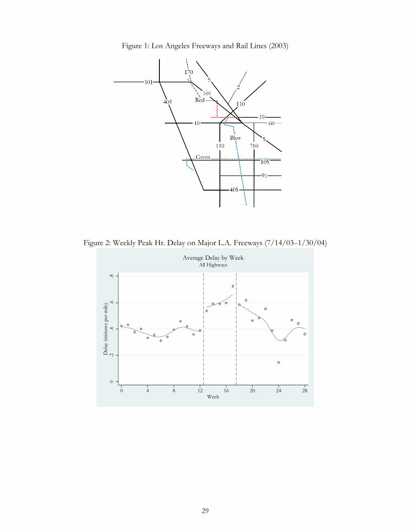
Figure 1: Los Angeles Freeways and Rail Lines (2003)

Figure 2: Weekly Peak Hr. Delay on Major L.A. Freeways (7/14/03–1/30/04)

0.2

.4.6

.8D

elay

(min

utes

per

mile

)

0 4 8 12 16 20 24 28Week

All HighwaysAverage Delay by Week

29

Figure 3: Weekly Peak Hr. Delay on Specific L.A. Freeways (7/14/03–1/30/04) Panel A: Red Line Freeway (US-101) Panel B: Green Line Freeway (I-105)

Panel C: Blue Line Freeways (I-110 & I-710) Panel D: Rapid 720 Freeway (I-10)

Figure 4: Weekly Peak Hr. Delay on Orange/Ventura County Freeways (7/14/03–1/30/04)

.2.4

.6.8

1D

elay

(min

utes

per

mile

)

0 4 8 12 16 20 24 28Week

US 101Average Delay by Week

.1.2

.3.4

.5.6

Del

ay (m

inut

es p

er m

ile)

0 4 8 12 16 20 24 28Week

Interstate 105Average Delay by Week

0.2

.4.6

.8D

elay

(min

utes

per

mile

)

0 4 8 12 16 20 24 28Week

Interstates 110 and 710Average Delay by Week

0.5

11.

5D

elay

(min

utes

per

mile

)

0 4 8 12 16 20 24 28Week

Interstate 10Average Delay by Week

0.2

.4.6

.8D

elay

(min

utes

per

mile

)

0 4 8 12 16 20 24 28Week

Control HighwaysAverage Delay by Week

30

Figure 5: Weekly Peak Hr. Delay on Major L.A. Freeways 1 Year Later (7/14/04–1/30/05)

0.2

.4.6

.8D

elay

(min

utes

per

mile

)

0 4 8 12 16 20 24 28Week

2004 Placebo Strike (All Highways)Average Delay by Week

Parameter Related variable Rail Bus Source (where applicable)General ParametersTrip Length m 7 miles 5 miles Parry and Small (2009)Hourly Wage (avg) vi BLS (2004)Hourly Wage (95% interval) vi BLS (2004)Wage Multiplier for Value of Time vi Parry and Small (2009)Delay Multiplier c Parry and Small (2009)

Transit Travel Time and CostsTransit Vehicle Speed (avg) sr , sb 23 mph 11 mph Parry and Small (2009)Transit Vehicle Speed (95% interval) sr , sb 23 mph 8.8–11.6 mphAvg Time Between Trains/Buses wr , wb 7 mins 8 mins Los Angeles County MTAWalking Speed ar , ab

Adult Fare (per mile) pr , pb $0.12 $0.17 Los Angeles County MTA

Driving Travel Time and CostsFree-flow Driving Speed sd 40 mph 35 mph Parry and Small (2009)Actual Driving Speed (avg) wd 30 mph 27.1 mph Parry and Small (2009)Actual Driving Speed (95% interval) wd 14 –40 mph 13.3–35 mph PeMS Data, Bing MapsAccess, Parking, and Egress Time ad

Operating Costs (per mile) pd AAA (2004)Share Commuters with Free Parking pd

Parking Costs (per day) pd

Notes: The delay multiplier applies to time spent waiting for transit, walking, or delayed in traffic. For timespent delayed in traffic, we calculate delay time as the difference between actual driving time and drivingtime under free-flow conditions.

Table 1: Parameter Values for Model Calibration

3 mins$0.1585%$5.00

0.5

$21.60$8.00–$65.50

1.8

2.5 mph

31

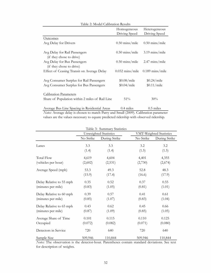
Homogeneous Driving Speed

Heterogeneous Driving Speed

OutcomesAvg Delay for Drivers 0.50 mins/mile 0.50 mins/mile

Avg Delay for Rail Passengers 0.50 mins/mile 3.19 mins/mile (if they chose to drive)Avg Delay for Bus Passengers 0.50 mins/mile 2.47 mins/mile (if they chose to drive)Effect of Ceasing Transit on Average Delay 0.032 mins/mile 0.189 mins/mile

Avg Consumer Surplus for Rail Passengers $0.08/mile $0.24/mileAvg Consumer Surplus for Bus Passengers $0.04/mile $0.11/mile

Calibration ParametersShare of Population within 2 miles of Rail Line 51% 30%

Average Bus Line Spacing in Residential Areas 0.4 miles 0.5 milesNotes: Average delay is chosen to match Parry and Small (2009). Calibration parametervalues are the values necessary to equate predicted ridership with observed ridership.

Table 2: Model Calibration Results

No Strike During Strike No Strike During Strike

Lanes 3.3 3.3 3.2 3.2(1.4) (1.4) (1.5) (1.5)

Total Flow 4,619 4,604 4,401 4,355(vehicles per hour) (2,602) (2,531) (2,730) (2,674)

Average Speed (mph) 53.3 49.3 52.8 48.3(15.9) (17.4) (16.6) (17.9)

Delay Relative to 55 mph 0.35 0.52 0.37 0.55(minutes per mile) (0.83) (1.05) (0.81) (1.01)

Delay Relative to 60 mph 0.39 0.57 0.41 0.61(minutes per mile) (0.85) (1.07) (0.83) (1.04)

Delay Relative to 65 mph 0.43 0.62 0.45 0.66(minutes per mile) (0.87) (1.09) (0.85) (1.05)

Average Share of Time 0.101 0.115 0.110 0.125Occupied (0.072) (0.082) (0.071) (0.080)

Detectors in Service 720 640 720 640

Sample Size 509,946 110,844 509,946 110,844

Table 3: Summary Statistics

Notes: The observation is the detector-hour. Parentheses contain standard deviations. See textfor description of weights.

VMT-Weighted StatisticsUnweighted Statistics

32

Dependent Variable: Average Delay (in minutes per mile)

(1) (2) (3) (4) (5) (6)

Strike 0.194 0.332 0.218 0.190 0.357 0.125(0.041) (0.076) (0.052) (0.051) (0.128) (0.042)

Date -0.004 -0.003 -0.002 -0.003 -0.005 -0.005(0.002) (0.003) (0.002) (0.002) (0.004) (0.002)

Date*Strike 0.007 0.006 -0.001 0.007 0.012 0.007(0.002) (0.003) (0.002) (0.003) (0.007) (0.002)

Average Delay Pre-Strike 0.409 0.369 0.264 0.357 0.600 0.434

Freeways All 101 105 110 & 710 10 Other

Parallel Transit Line Red Line Green Line Blue Line Rapid 720

Sample Size 178,549 15,854 31,058 19,152 15,357 97,128Notes: Each column represents a separate VMT-weighted regression, with weights equal to (length of highway coveredby detector i)*(average pre-strike traffic flow over detector i). The observation is the detector-hour, and the sample islimited to weekdays from 7-10 am and 2-8 pm within 28 days of the strike's beginning. Parentheses contain clusteredstandard errors that are robust to within-day and within-detector serial correlation. All regressions include day-of-week and detector fixed effects.

Table 4: Effect of Strike on Delays During All Peak Hours

33

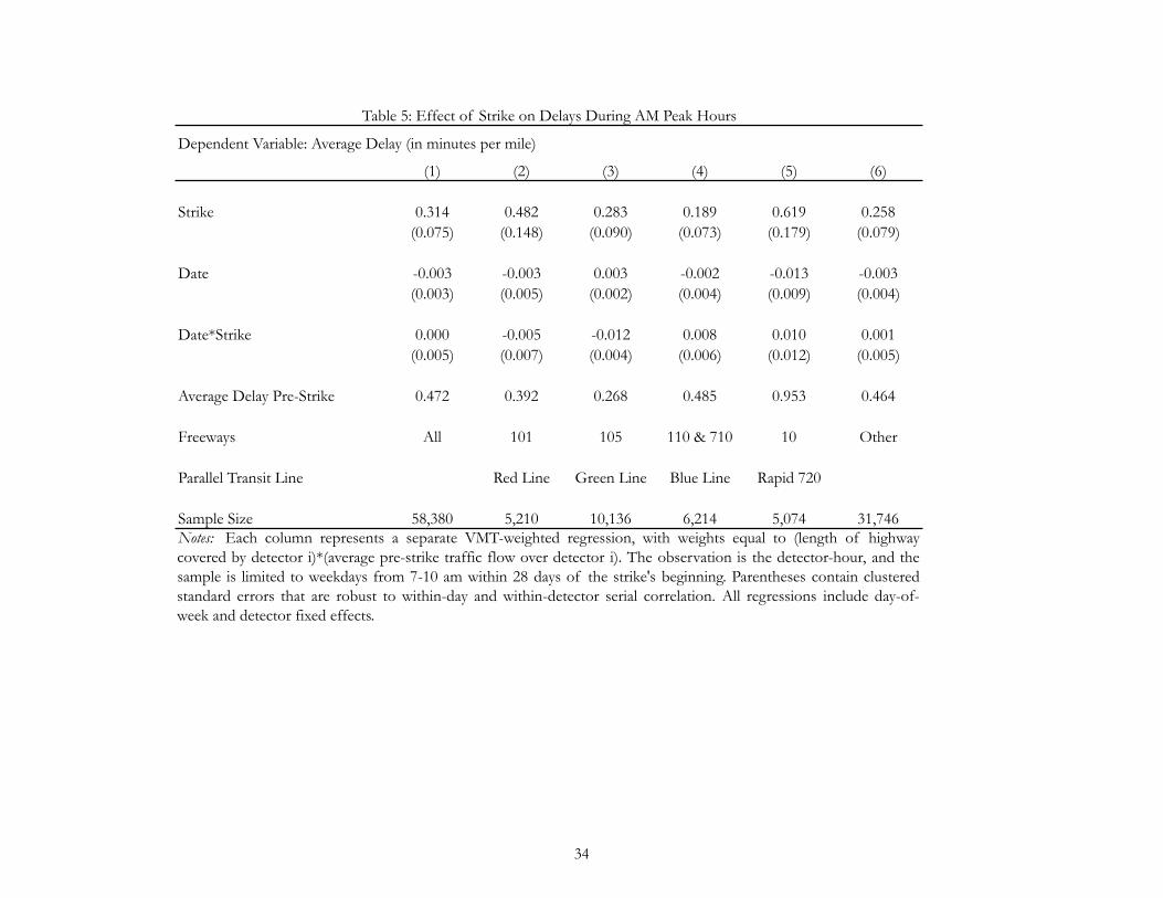
Dependent Variable: Average Delay (in minutes per mile)

(1) (2) (3) (4) (5) (6)

Strike 0.314 0.482 0.283 0.189 0.619 0.258(0.075) (0.148) (0.090) (0.073) (0.179) (0.079)

Date -0.003 -0.003 0.003 -0.002 -0.013 -0.003(0.003) (0.005) (0.002) (0.004) (0.009) (0.004)

Date*Strike 0.000 -0.005 -0.012 0.008 0.010 0.001(0.005) (0.007) (0.004) (0.006) (0.012) (0.005)

Average Delay Pre-Strike 0.472 0.392 0.268 0.485 0.953 0.464

Freeways All 101 105 110 & 710 10 Other

Parallel Transit Line Red Line Green Line Blue Line Rapid 720

Sample Size 58,380 5,210 10,136 6,214 5,074 31,746

Table 5: Effect of Strike on Delays During AM Peak Hours

Notes: Each column represents a separate VMT-weighted regression, with weights equal to (length of highwaycovered by detector i)*(average pre-strike traffic flow over detector i). The observation is the detector-hour, and thesample is limited to weekdays from 7-10 am within 28 days of the strike's beginning. Parentheses contain clusteredstandard errors that are robust to within-day and within-detector serial correlation. All regressions include day-of-week and detector fixed effects.

34

Dependent Variable: Average Delay (in minutes per mile)

(1) (2) (3) (4) (5) (6)

Strike 0.157 0.266 0.213 0.197 0.279 0.085(0.040) (0.064) (0.061) (0.056) (0.132) (0.049)

Date -0.005 -0.004 -0.005 -0.004 -0.004 -0.006(0.002) (0.003) (0.002) (0.002) (0.005) (0.002)

Date*Strike 0.010 0.011 0.005 0.007 0.017 0.011(0.002) (0.004) (0.002) (0.002) (0.008) (0.002)

Average Delay Pre-Strike 0.384 0.361 0.274 0.300 0.401 0.431

Freeways All 101 105 110 & 710 10 Other

Parallel Transit Line Red Line Green Line Blue Line Rapid 720

Sample Size 120,007 10,575 20,922 12,938 10,283 65,289

Table 6: Effect of Strike on Delays During PM Peak Hours

Notes: Each column represents a separate VMT-weighted regression, with weights equal to (length of highwaycovered by detector i)*(average pre-strike traffic flow over detector i). The observation is the detector-hour, and thesample is limited to weekdays from 2-8 pm within 28 days of the strike's beginning. Parentheses contain clusteredstandard errors that are robust to within-day and within-detector serial correlation. All regressions include day-of-week and detector fixed effects.

35

Dependent Variable: Average Share of Time Detector Is Occupied

(1) (2) (3) (4) (5) (6)

Strike 0.013 0.023 0.019 0.016 0.022 0.008(0.003) (0.006) (0.004) (0.004) (0.009) (0.003)

Date 0.000 0.000 0.000 0.000 0.000 0.000(0.000) (0.000) (0.000) (0.000) (0.000) (0.000)

Date*Strike 0.000 0.000 0.000 0.000 0.001 0.000(0.000) (0.000) (0.000) (0.000) (0.000) (0.000)

Average Share of Time Detector 0.112 0.121 0.097 0.115 0.129 0.110 Is Occupied Pre-StrikeFreeways All 101 105 110 & 710 10 Other

Parallel Transit Line Red Line Green Line Blue Line Rapid 720

Sample Size 179,680 16,222 31,112 19,152 15,668 97,526

Table 7: Effect of Strike on Freeway Occupancy

Notes: Each column represents a separate VMT-weighted regression, with weights equal to (length of highway coveredby detector i)*(lanes at detector i). The observation is the detector-hour, and the sample is limited to weekdays from 7-10 am and 2-8 pm within 28 days of the strike's beginning. Parentheses contain clustered standard errors that arerobust to within-day and within-detector serial correlation. All regressions include day-of-week and detector fixedeffects.

36

Dependent Variable: Hourly Traffic Flow per Lane

(1) (2) (3) (4) (5) (6)

Strike -31.3 -68.2 -9.4 -1.4 -61.1 -29.4(9.7) (17.3) (11.7) (18.1) (19.6) (9.0)

Date 0.81 0.79 0.91 0.46 1.14 0.83(0.40) (0.58) (0.62) (0.94) (0.88) (0.33)

Date*Strike -1.85 -2.50 -1.29 -2.46 -2.45 -1.53(0.61) (0.85) (0.73) (1.07) (1.06) (0.60)

Average Hourly Flow Pre-Strike 1,399 1,576 1,349 1,403 1,455 1,353

Freeways All 101 105 110 & 710 10 Other

Parallel Transit Line Red Line Green Line Blue Line Rapid 720

Sample Size 179,680 16,222 31,112 19,152 15,668 97,526

Table 8: Effect of Strike on Traffic Flows

Notes: Each column represents a separate VMT-weighted regression, with weights equal to (length of highway coveredby detector i)*(lanes at detector i). The observation is the detector-hour, and the sample is limited to weekdays from 7-10 am and 2-8 pm within 28 days of the strike's beginning. Parentheses contain clustered standard errors that arerobust to within-day and within-detector serial correlation. All regressions include day-of-week and detector fixedeffects.

37

Dependent Variable: Average Delay (in minutes per mile)

Falsification Sample:(1) (2) (3) (4) (5) (6)

Strike 0.024 0.025 0.026 0.060 0.082 0.045(0.027) (0.037) (0.037) (0.042) (0.054) (0.064)

Date 0.000 -0.001 0.000 -0.002 -0.002 -0.003(0.001) (0.003) (0.002) (0.002) (0.003) (0.002)

Date*Strike 0.004 0.000 0.006 0.005 0.002 0.007(0.002) (0.003) (0.003) (0.003) (0.003) (0.004)

Average Delay Pre-Strike 0.205 0.170 0.219 0.433 0.539 0.386

Hours All Peak AM Peak PM Peak All Peak AM Peak PM Peak

Sample Size 13,149 4,296 8,853 177,572 59,532 118,034

Table 9: Effect of Placebo Strikes on Delays

Notes: Each column represents a separate VMT-weighted regression, with weights equal to (length of highway covered bydetector i)*(average pre-strike traffic flow over detector i). The observation is the detector-hour, and the sample is limitedto weekdays from 7-10 am and 2-8 pm within 28 days of the strike's beginning. Parentheses contain clustered standarderrors that are robust to within-day and within-detector serial correlation. All regressions include day-of-week and detectorfixed effects. In Columns (1)-(3) the strike variable is defined normally but the sample contains detectors in neighboringcounties not subject to the strike. In columns (4)-(6) the strike variable equals zero prior to October 12, 2004 and unityafter October 12, 2004.

Orange and Ventura Counties October/November 2004

38

Travel Response Parameter

Implied generalized travel cost elasticity

of VMT

Lightly-affected freeways

Average freeway

Heavily-affected freeways

Lightly-affected freeways

Average freeway

Heavily-affected freeways

Panel A: Delay Multiplier = 1.8, Arterial CongestionFuel price elasticity of VMT = -0.15 -0.67 -2.5% -3.9% -6.7% 63% 62% 56% $2.6 billion

Fuel price elasticity of VMT = -0.34 -1.5 -3.3% -5.2% -8.9% 51% 49% 45% $2.1 billion

London Congestion Charge Response -2.0 -3.6% -5.7% -9.7% 46% 45% 40% $1.9 billion

Panel B: No Delay Multiplier, No Arterial CongestionFuel price elasticity of VMT = -0.15 -0.67 -0.8% -1.5% -2.5% 87% 85% 81% $1 billion

Fuel price elasticity of VMT = -0.34 -1.5 -1.3% -2.1% -3.7% 80% 79% 74% $1 billion

London Congestion Charge Response -2.0 -1.5% -2.5% -4.3% 77% 75% 70% $1 billion

Long-run equilibrium travel demand reduction Long-run effect as a % of short-run effectTable 10: Potential Long-run Effects

Notes: Panel A applies a delay multiplier of 1.8 to time spent in traffic and assumes an effect of transit on arterial congestion that is similar to the estimated effect of transit on freeway congestion. Panel B applies no delay multiplier and assumes transit has no effect on arterial congestion.

Long-run annual

congestion relief benefit

39

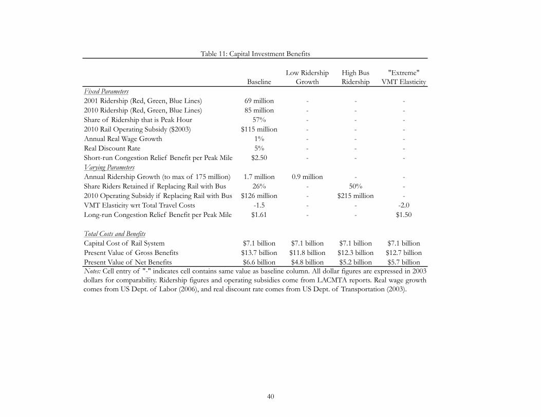
BaselineLow Ridership

GrowthHigh Bus Ridership

"Extreme" VMT Elasticity

Fixed Parameters2001 Ridership (Red, Green, Blue Lines) 69 million - - -2010 Ridership (Red, Green, Blue Lines) 85 million - - -Share of Ridership that is Peak Hour 57% - - -2010 Rail Operating Subsidy ($2003) $115 million - - -Annual Real Wage Growth 1% - - -Real Discount Rate 5% - - -Short-run Congestion Relief Benefit per Peak Mile $2.50 - - -Varying ParametersAnnual Ridership Growth (to max of 175 million) 1.7 million 0.9 million - -Share Riders Retained if Replacing Rail with Bus 26% - 50% -2010 Operating Subsidy if Replacing Rail with Bus $126 million - $215 million -VMT Elasticity wrt Total Travel Costs -1.5 - - -2.0Long-run Congestion Relief Benefit per Peak Mile $1.61 - - $1.50

Total Costs and BenefitsCapital Cost of Rail System $7.1 billion $7.1 billion $7.1 billion $7.1 billionPresent Value of Gross Benefits $13.7 billion $11.8 billion $12.3 billion $12.7 billionPresent Value of Net Benefits $6.6 billion $4.8 billion $5.2 billion $5.7 billion

Table 11: Capital Investment Benefits

Notes: Cell entry of "-" indicates cell contains same value as baseline column. All dollar figures are expressed in 2003dollars for comparability. Ridership figures and operating subsidies come from LACMTA reports. Real wage growthcomes from US Dept. of Labor (2006), and real discount rate comes from US Dept. of Transportation (2003).

40

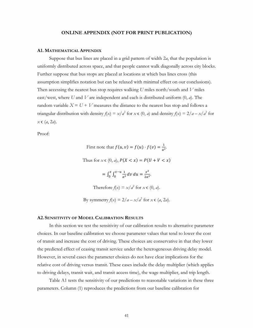
ONLINE APPENDIX (NOT FOR PRINT PUBLICATION)

A1. MATHEMATICAL APPENDIX

Suppose that bus lines are placed in a grid pattern of width 2a, that the population is

uniformly distributed across space, and that people cannot walk diagonally across city blocks.

Further suppose that bus stops are placed at locations at which bus lines cross (this

assumption simplifies notation but can be relaxed with minimal effect on our conclusions).

Then accessing the nearest bus stop requires walking U miles north/south and V miles

east/west, where U and V are independent and each is distributed uniform (0, a). The

random variable X = U + V measures the distance to the nearest bus stop and follows a

triangular distribution with density f(x) = x/a2 for x ϵ (0, a) and density f(x) = 2/a – x/a2 for

x ϵ (a, 2a).

Proof:

First note that ! !, ! = !(!) ⋅ !(!) = !!!.

Thus for x ϵ (0, a), ! ! < ! = ! ! + ! < !

= !!! !" !"

!!!!

!! = !!

!!!.

Therefore f(x) = x/a2 for x ϵ (0, a).

By symmetry f(x) = 2/a – x/a2 for x ϵ (a, 2a).

A2. SENSITIVITY OF MODEL CALIBRATION RESULTS

In this section we test the sensitivity of our calibration results to alternative parameter

choices. In our baseline calibration we choose parameter values that tend to lower the cost

of transit and increase the cost of driving. These choices are conservative in that they lower

the predicted effect of ceasing transit service under the heterogeneous driving delay model.

However, in several cases the parameter choices do not have clear implications for the

relative cost of driving versus transit. These cases include the delay multiplier (which applies

to driving delays, transit wait, and transit access time), the wage multiplier, and trip length.

Table A1 tests the sensitivity of our predictions to reasonable variations in these three

parameters. Column (1) reproduces the predictions from our baseline calibration for

41

comparison purposes. In the baseline calibration, the heterogeneous driving delay model

predicts a congestion impact from ceasing transit service that is 5.9 times greater than the

homogeneous driving delay model’s prediction. Columns (2) and (3) test sensitivity to

variations in the delay multiplier, which is set at c = 1.8 in our baseline calibration (a delay

multiplier of 1.8 implies that individuals value time spent waiting in traffic, waiting for transit,

or walking to transit at 1.8 times their normal value of time). Under a high delay multiplier (c

= 2.3), the ratio of the heterogeneous model prediction to the homogeneous model

prediction increases to 7.7. Under a low delay multiplier (c = 1.3), the ratio decreases to 3.4.

Columns (4) and (5) test sensitivity to variations in the value of time. Under a high value of

time (60% of the average wage), the ratio of the two models’ predictions increases to 7.6.

Under a low value of time (40% of the average wage), the ratio decreases to 4.1. Columns (6)

and (7) test sensitivity to variations in trip length. Since long and short trips are less common

than average-length trips, we calibrate the model in these two columns so that predicted

transit share is half the overall transit share. This reduces the predicted impact of ceasing

transit service under either model (homogeneous or heterogeneous), but it has little impact

on the ratio of the two predictions (which is the object of interest). On long trips (a 10-mile

rail trip or a 7-mile bus trip), the ratio of the two predictions is 6.1. On short trips (a 5-mile

rail trip or a 3-mile bus trip), the ratio of the two predictions is 3.6.

Table A2 tests the sensitivity of our predictions to different assumptions about

transportation alternatives and sorting behavior. Column (1) reproduces the predictions

from our baseline calibration for comparison purposes. Column (2) calibrates the two

models under the assumption that one-third of the bus riders are “captive” riders who do

not own cars. Under this assumption the predicted impact of ceasing transit service falls in

both models because captive riders do not switch to driving. Nevertheless, the ratio of the

two models’ predictions is nearly unchanged at 6.1. Column (3) calibrates the two models

under the assumption that access time and driving delays are negatively correlated (i.e.,

people living far from transit experience fewer driving delays). This modification captures

the possibility that denser areas have better transit access and more congestion. The ratio of

the two predictions increases to 6.5. Column (4) calibrates the two models under the

assumption that access time and value of time are positively correlated (i.e., wealthy

neighborhoods are farther from transit). This modification captures the possibility that low-

income individuals choose to live closer to transit. The ratio of the two predictions decreases

to 4.6.

42

Two patterns emerge from the sensitivity analyses in Tables A1 and A2. First, in all

cases the heterogeneous driving delay model predicts a much greater increase in congestion

from ceasing transit service than the homogeneous driving delay model. The minimum ratio

between the two models’ predictions is 3.4, and the maximum ratio is 7.7. Second, despite

the consistent qualitative finding that a model incorporating heterogeneous driving delays

predicts much greater congestion impacts, the magnitude of the predictions varies

substantially with different parameter values. Thus it is infeasible to make an accurate

quantitative prediction about the effect of ceasing transit service without additional data or a

natural experiment.

43

(1) (2) (3) (4) (5) (6) (7)Parameter Modification: None High Delay Low Delay High Value Low Value Long Trip Short Trip

Multiplier Multiplier of Time of Time (Rail = 10 miles, (Rail = 5 miles,(c = 2.3) (c = 1.3) (60% avg wage) (40% avg wage) Bus = 7 miles) Bus = 3 miles)

OutcomesEffect of Ceasing Transit on Average Delay 6.3% 6.4% 6.4% 6.3% 6.3% 3.1% 3.1% (Homogeneous Driving Delay Model)Effect of Ceasing Transit on Average Delay 37.1% 49.3% 21.5% 47.8% 25.8% 18.9% 11.2% (Heterogeneous Driving Delay Model)Ratio of Heterogeneous Model Effect 5.9 7.7 3.4 7.6 4.1 6.1 3.6 to Homogeneous Model Effect

Calibration Parameters (Heterogeneous Model)Share of Population within 2 miles of Rail Line 30% 30% 27% 32% 25% 15% 30%

Average Bus Line Spacing in Residential Areas 0.5 miles 0.5 miles 0.5 miles 0.3 miles 0.7 miles 0.6 miles 0.6 miles

Table A1: Model Calibration Results Under Different Parameter Values

Notes: Average delay is chosen to match Parry and Small (2009). Calibration parameter values are the values necessary to equate predicted ridership with observed ridership inthe model with heterogeneous driving delays. The effect of ceasing transit under the homogeneous model is smaller in columns (6) and (7) than other columns becauseobserved ridership for long/short trips is assumed to be half the observed ridership for the average trip.

44

(1) (2) (3) (4) (5)Parameter Modification: None 1/3 of Bus Riders Access Time and Delays Access Time and Value Bus Access Time

are "Captive" Negatively Correlated of Time Positively DistributedCorrelated Gamma

OutcomesEffect of Ceasing Transit on Average Delay 6.3% 4.7% 6.3% 6.2% 6.2% (Homogeneous Driving Delay Model)Effect of Ceasing Transit on Average Delay 37.1% 28.6% 41.0% 28.5% 33.7% (Heterogeneous Driving Delay Model)Ratio of Heterogeneous Model Effect 5.9 6.1 6.5 4.6 5.4 to Homogeneous Model Effect

Calibration Parameters (Heterogeneous Model)Share of Population within 2 miles of Rail Line 30% 30% 28% 22% 30%

Average Bus Line Spacing in Residential Areas 0.5 miles 0.5 miles 0.5 miles 0.7 miles 0.5 miles

Table A2: Model Calibration Results Under Different Parameter Values

Notes: Average delay is chosen to match Parry and Small (2009). Calibration parameter values are the values necessary to equate predicted ridership with observed ridership in the model with heterogeneous driving delays. The effect of ceasing transit under the homogeneous model is smaller in column (2) than other columns because the "captive" riders do not switch to driving when transit service ceases.

45

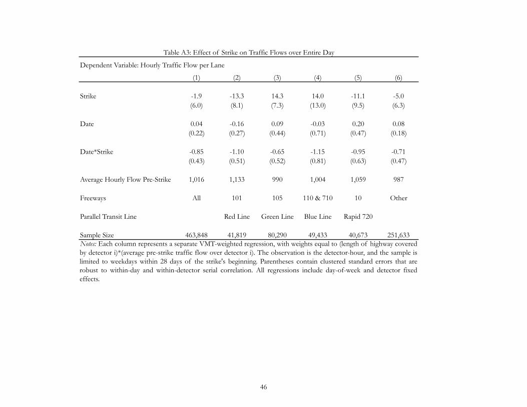
Dependent Variable: Hourly Traffic Flow per Lane

(1) (2) (3) (4) (5) (6)

Strike -1.9 -13.3 14.3 14.0 -11.1 -5.0(6.0) (8.1) (7.3) (13.0) (9.5) (6.3)

Date 0.04 -0.16 0.09 -0.03 0.20 0.08(0.22) (0.27) (0.44) (0.71) (0.47) (0.18)

Date*Strike -0.85 -1.10 -0.65 -1.15 -0.95 -0.71(0.43) (0.51) (0.52) (0.81) (0.63) (0.47)

Average Hourly Flow Pre-Strike 1,016 1,133 990 1,004 1,059 987

Freeways All 101 105 110 & 710 10 Other

Parallel Transit Line Red Line Green Line Blue Line Rapid 720

Sample Size 463,848 41,819 80,290 49,433 40,673 251,633

Table A3: Effect of Strike on Traffic Flows over Entire Day

Notes: Each column represents a separate VMT-weighted regression, with weights equal to (length of highway coveredby detector i)*(average pre-strike traffic flow over detector i). The observation is the detector-hour, and the sample islimited to weekdays within 28 days of the strike's beginning. Parentheses contain clustered standard errors that arerobust to within-day and within-detector serial correlation. All regressions include day-of-week and detector fixedeffects.

46