Subsurface Inverse Modeling with Physics Based Machine

Subsurface Inverse Modeling with Physics BasedMachine Learning

Kailai Xu and Dongzhuo LiJerry M. Harris, Eric Darve

Kailai Xu ([email protected]), et al. Physics Constrained Learning 1 / 35

Outline

1 Inverse Modeling

2 Automatic Differentiation

3 Physics Constrained Learning

4 Applications

5 ADCME: Scientific Machine Learning for Inverse Modeling


Inverse Modeling

Inverse modeling identifies a certain set of parameters or functionswith which the outputs of the forward analysis matches the desiredresult or measurement.

Many real life engineering problems can be formulated as inversemodeling problems: shape optimization for improving the performanceof structures, optimal control of fluid dynamic systems, etc.t

Physical Properties

Physical Laws

Predictions (Observations)

Inverse Modeling

……

Optimal Control

Predictive Modeling

Discover Physics

Reduced Order Modeling


Inverse Modeling

Forward Problem

Inverse Problem

Model Parameters

Observations

Physical Laws

Physical LawsEstimation

of Parameters

Prediction of

Observations


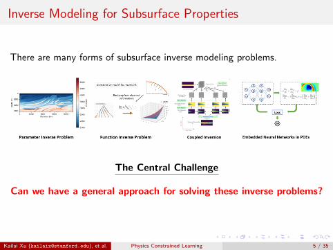
Inverse Modeling for Subsurface Properties

There are many forms of subsurface inverse modeling problems.

The Central Challenge

Can we have a general approach for solving these inverse problems?


Parameter Inverse Problem

We can formulate inverse modeling as a PDE-constrained optimizationproblem

minθ

Lh(uh) s.t. Fh(θ, uh) = 0

The loss function Lh measures the discrepancy between the predictionuh and the observation uobs, e.g., Lh(uh) = ‖uh − uobs‖2

2.

θ is the model parameter to be calibrated.

The physics constraints Fh(θ, uh) = 0 are described by a system ofpartial differential equations. Solving for uh may require solving linearsystems or applying an iterative algorithm such as theNewton-Raphson method.


Function Inverse Problem

minf

Lh(uh) s.t. Fh(f , uh) = 0

What if the unknown is a function instead of a set of parameters?

Koopman operator in dynamical systems.Constitutive relations in solid mechanics.Turbulent closure relations in fluid mechanics.Neural-network-based physical properties....

The candidate solution space is infinite dimensional.


Physics Based Machine Learning

minθ

Lh(uh) s.t. Fh(NNθ, uh) = 0

Deep neural networks exhibit capability of approximating highdimensional and complicated functions.Physics based machine learning: the unknown function isapproximated by a deep neural network, and the physical constraintsare enforced by numerical schemes.Satisfy the physics to the largest extent.


Gradient Based Optimization

minθ

Lh(uh) s.t. Fh(θ, uh) = 0 (1)

We can now apply a gradient-based optimization method to (1).The key is to calculate the gradient descent direction gk

θk+1 ← θk − αgk

Predicted Data

Observed Data

Loss Function

Calculate Gradients

Update Model Parameters

PDE

Initial and Boundary Conditions

Optimizer

< tol?Calibrated Model


Outline

1 Inverse Modeling



4 Applications



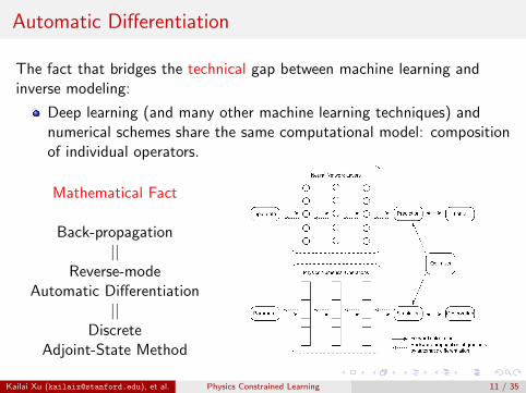
Automatic Differentiation

The fact that bridges the technical gap between machine learning andinverse modeling:

Deep learning (and many other machine learning techniques) andnumerical schemes share the same computational model: compositionof individual operators.

Mathematical Fact

Back-propagation||

Reverse-modeAutomatic Differentiation

||Discrete

Adjoint-State Method


Forward Mode vs. Reverse Mode

Reverse mode automatic differentiation evaluates gradients in thereverse order of forward computation.Reverse mode automatic differentiation is a more efficient way tocompute gradients of a many-to-one mapping J(α1, α2, α3, α4) ⇒suitable for minimizing a loss (misfit) function.


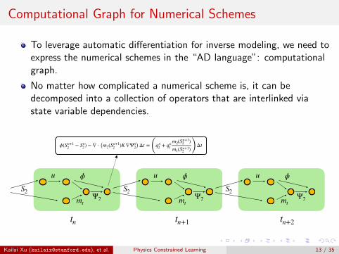
Computational Graph for Numerical Schemes

To leverage automatic differentiation for inverse modeling, we need toexpress the numerical schemes in the “AD language”: computationalgraph.

No matter how complicated a numerical scheme is, it can bedecomposed into a collection of operators that are interlinked viastate variable dependencies.

S2

u ϕ

mtΨ2

ϕ(Sn+12 − Sn2) − ∇ ⋅ (m2(Sn+1

2 )K ∇Ψn2) Δt = (qn2 + qn1m2(Sn+12 )m1(Sn+12 ) ) Δt

S2

u ϕ

mtΨ2

S2

u ϕ

mtΨ2

tn tn+1 tn+2


Outline

1 Inverse Modeling



4 Applications



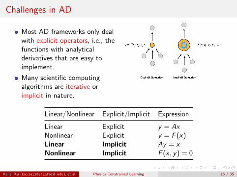
Challenges in AD

Most AD frameworks only dealwith explicit operators, i.e., thefunctions with analyticalderivatives that are easy toimplement.

Many scientific computingalgorithms are iterative orimplicit in nature.

Linear/Nonlinear Explicit/Implicit Expression

Linear Explicit y = AxNonlinear Explicit y = F (x)Linear Implicit Ay = xNonlinear Implicit F (x , y) = 0


Implicit Operators in Subsurface Modeling

For reasons such as nonlinearity and stability, implicit operators(schemes) are almost everywhere in subsurface modeling...

The ultimate solution: design “differentiable” implicit operators.


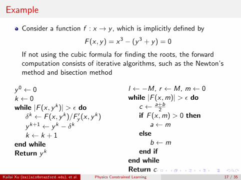
Example

Consider a function f : x → y , which is implicitly defined by

F (x , y) = x3 − (y3 + y) = 0

If not using the cubic formula for finding the roots, the forwardcomputation consists of iterative algorithms, such as the Newton’smethod and bisection method

y0 ← 0k ← 0while |F (x , yk)| > ε do

δk ← F (x , yk)/F ′y (x , yk)

yk+1 ← yk − δkk ← k + 1

end whileReturn yk

l ← −M, r ← M, m← 0while |F (x ,m)| > ε do

c ← a+b2

if F (x ,m) > 0 thena← m

elseb ← m

end ifend whileReturn c


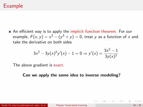
Example

An efficient way is to apply the implicit function theorem. For ourexample, F (x , y) = x3 − (y3 + y) = 0, treat y as a function of x andtake the derivative on both sides

3x2 − 3y(x)2y ′(x)− 1 = 0⇒ y ′(x) =3x2 − 1

3y(x)2

The above gradient is exact.

Can we apply the same idea to inverse modeling?


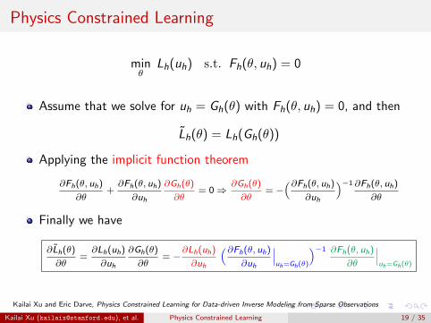
Physics Constrained Learning

minθ

Lh(uh) s.t. Fh(θ, uh) = 0

Assume that we solve for uh = Gh(θ) with Fh(θ, uh) = 0, and then

L̃h(θ) = Lh(Gh(θ))

Applying the implicit function theorem

∂Fh(θ, uh)

∂θ+∂Fh(θ, uh)

∂uh

∂Gh(θ)

∂θ= 0⇒

∂Gh(θ)

∂θ= −

(∂Fh(θ, uh)

∂uh

)−1 ∂Fh(θ, uh)

∂θ

Finally we have

∂L̃h(θ)

∂θ=∂Lh(uh)

∂uh

∂Gh(θ)

∂θ= −

∂Lh(uh)

∂uh

(∂Fh(θ, uh)

∂uh

∣∣∣uh=Gh(θ)

)−1 ∂Fh(θ, uh)

∂θ

∣∣∣uh=Gh(θ)

Kailai Xu and Eric Darve, Physics Constrained Learning for Data-driven Inverse Modeling from Sparse Observations


Outline

1 Inverse Modeling



4 Applications



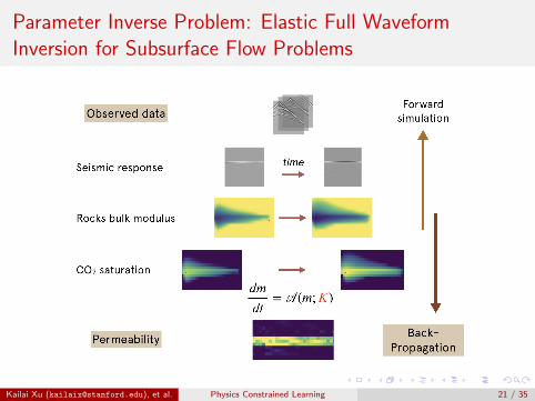
Parameter Inverse Problem: Elastic Full WaveformInversion for Subsurface Flow Problems


Fully Nonlinear Implicit Schemes

The governing equation is a nonlinear PDE

∂

∂t(φSiρi ) +∇ · (ρivi ) = ρiqi , i = 1, 2

S1 + S2 = 1

vi = −Kkri

µ̃i(∇Pi − gρi∇Z), i = 1, 2

kr1(S1) =kor1S

L11

SL11 + E1S

T12

kr2(S1) =SL2

2

SL22 + E2S

T21

ρ∂vz

∂t=∂σzz

∂z+∂σxz

∂x

ρ∂vx

∂t=∂σxx

∂x+∂σxz

∂z∂σzz

∂t= (λ+ 2µ)

∂vz

∂z+ λ

∂vx

∂x∂σxx

∂t= (λ+ 2µ)

∂vx

∂x+ λ

∂vz

∂z∂σxz

∂t= µ(

∂vz

∂x+∂vx

∂z),

For stability and efficiency, implicit methods are the industrialstandards.

φ(Sn+12 − Sn

2 )−∇ ·(m2(Sn+1

2 )K∇Ψn2

)∆t =

(qn2 + qn1

m2(Sn+12 )

m1(Sn+12 )

)∆t mi (s) =

kri (s)

µ̃i


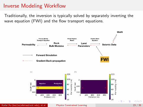
Inverse Modeling Workflow

Traditionally, the inversion is typically solved by separately inverting thewave equation (FWI) and the flow transport equations.


Coupled Inversion vs. Decoupled Inversion

We found that coupled inversion reduces the artifacts from FWIsignificantly and yields a substantially better results.


Travel Time vs. Full Waveforms

We also compared using only travel time (left, Eikonal equation) versususing full waveforms (right, FWI) for inversion. We found that fullwaveforms do contain more information for making a better estimation ofthe permeability property.

The Eikonal equation solver was also implemented with physics constrained

learning!


Check out our package FwiFlow.jl for wave and flow inversion and ourrecently published paper for this work.

High Performance

Solves inverse modelingproblems faster with ourGPU-accelerated FWImodule.

Designed forSubsurface Modeling

Provides many operatorsthat can be reused fordifferent subsurfacemodeling problems.

Easy to Extend

Allows users toimplement and inserttheir own customoperators and solve newproblems.


Function Inverse Problem: Modeling Viscoelasticity

Multi-physics Interaction of Coupled Geomechanics and Multi-PhaseFlow Equations

divσ(u)− b∇p = 0

1

M

∂p

∂t+ b

∂εv (u)

∂t−∇ ·

(k

Bf µ∇p)

= f (x , t)

σ = σ(ε, ε̇)

Approximate the constitutive relation by a neural network

σn+1 = NN θ(σn, εn) + Hεn+1

Traction-free∂u∂n

= 0

No-flow∂p∂n

= 0

Fixed Pressurep = 0

No-flow∂p∂n

= 0No-flow∂p∂n

= 0 Injection Production

x

y

Finite Element Finite Volume Cell

He1 He2

He3 He4

e

Sensors


Neural Networks: Inverse Modeling of Viscoelasticity

We propose the following form for modeling viscosity (assume thetime step size is fixed):

σn+1 − σn = NN θ(σn, εn) + H(εn+1 − εn)

H is a free optimizable symmetric positive definite matrix (SPD).Hence the numerical stiffness matrix is SPD.

Implicit linear equation

σn+1 − Hεn+1 = −Hεn +NN θ(σn, εn) + σn := NN ∗θ(σn, εn)

Linear system to solve in each time step ⇒ good balance betweennumerical stability and computational cost.

Good performance in our numerical examples.


Training Strategy and Numerical Stability

Physics constrained learning = improved numerical stability inpredictive modeling.

For simplicity, consider two strategies to train an NN-basedconstitutive relation using direct data {(εno , σno)}n

∆σn = H∆εn +NN θ(σn, εn), H � 0

Training with input-output pairs

minθ

∑n

(σn+1o −

(Hεn+1

o +NN ∗θ(σno , εno)))2

Better stability using training on trajectory = physics constrainedlearning

minθ

∑n

(σn(θ)− σno)2

s.t. I.C. σ1 = σ1o and time integrator ∆σn = H∆εn +NN θ(σn, εn)


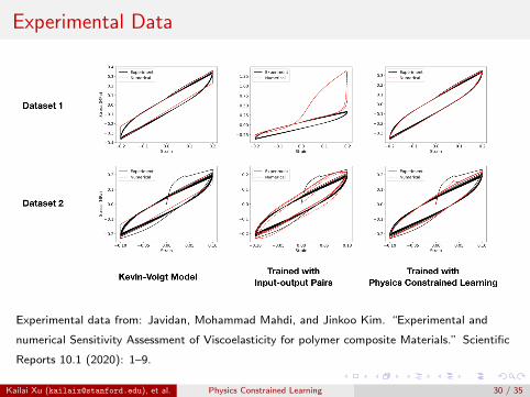
Experimental Data

Experimental data from: Javidan, Mohammad Mahdi, and Jinkoo Kim. “Experimental and

numerical Sensitivity Assessment of Viscoelasticity for polymer composite Materials.” Scientific

Reports 10.1 (2020): 1–9.


Inverse Modeling of Viscoelasticity

Comparison with space varying linear elasticity approximation

σ = H(x , y)ε


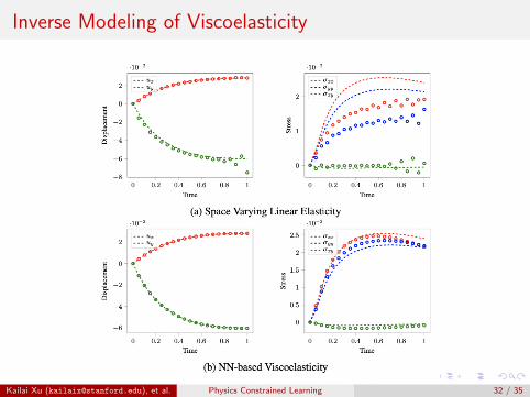
Inverse Modeling of Viscoelasticity


Outline

1 Inverse Modeling



4 Applications



Physical Simulation as a Computational Graph


A General Approach to Inverse Modeling


Documents

Subsurface Inverse Modeling with Physics Based Machine