Embed Size (px)
Citation preview

The Annals of Probability2017, Vol. 45, No. 1, 4–55DOI: 10.1214/15-AOP1030© Institute of Mathematical Statistics, 2017
SUBSEQUENTIAL SCALING LIMITS OF SIMPLE RANDOM WALKON THE TWO-DIMENSIONAL UNIFORM SPANNING TREE
BY M. T. BARLOW1, D. A. CROYDON2 AND T. KUMAGAI3
University of British Columbia, University of Warwick and Kyoto University
The first main result of this paper is that the law of the (rescaled) two-dimensional uniform spanning tree is tight in a space whose elements aremeasured, rooted real trees continuously embedded into Euclidean space.Various properties of the intrinsic metrics, measures and embeddings of thesubsequential limits in this space are obtained, with it being proved in partic-ular that the Hausdorff dimension of any limit in its intrinsic metric is almostsurely equal to 8/5. In addition, the tightness result is applied to deduce thatthe annealed law of the simple random walk on the two-dimensional uniformspanning tree is tight under a suitable rescaling. For the limiting processes,which are diffusions on random real trees embedded into Euclidean space,detailed transition density estimates are derived.
1. Introduction. The study of uniform spanning trees (USTs) has a long his-tory; in the 1840s Kirchhoff used them in his classic paper [34] on electrical re-sistance. Much of the recent theory in the probability literature is based on thediscovery that paths in the UST have the same law as loop erased random walks.Using this connection, algorithms to construct the UST from random walks havebeen given in [5, 14, 49]. See [12] for a survey of the properties of the UST, anda description of Wilson’s algorithm, which will be important for this article, and[38] for a survey of the properties of the loop erased random walk (LERW). Wealso remark that USTs can be considered as a boundary case of the random clustermodel; see [29].
In [48], Schramm studied the scaling limit of the UST in Z2, and this led himto introduce the SLE process. In [41], it was proved that the LERW in Z2 hasSLE2 as its scaling limit, and this connection was used in [10, 45] to improveearlier results of Kenyon [31] on the growth function of two-dimensional LERW.In [11], this good control on the length of LERW paths, combined with Wilson’salgorithm, was used to obtain volume growth and resistance estimates for the two-dimensional UST U . Using the connection between random walks and electrical
Received July 2014; revised April 2015.1Supported in part by NSERC (Canada).2Supported in part by EPSRC First Grant EP/K029657/1.3Supported in part by the JSPS Grant-in-Aid for Scientific Research (A) 25247007.MSC2010 subject classifications. 60D05, 60G57, 60J60, 60J67, 60K37.Key words and phrases. Uniform spanning tree, loop-erased random walk, random walk, scaling
limit, continuum random tree.
4

RANDOM WALK ON THE UNIFORM SPANNING TREE 5
resistance, and the methods of [9, 37], these bounds then led to heat kernel boundsfor U .
In this paper, we study scaling limits of U , as well as the random walk on it.While very significant progress in this direction was made on the first topic in [2,48], those papers are focused on the topological properties of the scaling limit as asubset of R2. Here, we work in a framework that allows us to describe propertiesof the joint scaling limit of the corresponding intrinsic metric, uniform measureand simple random walk.
We begin by introducing our main notation. Throughout this article, U will rep-resent the uniform spanning tree on Z2, and P the probability measure on the prob-ability space on which this is built. As proved in [47], U is the local limit of theuniform spanning tree on [−n,n]2 ∩Z2 (equipped with nearest-neighbour bonds)as n → ∞. We note that U is P-a.s. indeed a spanning tree of Z2, that is, it is agraph with vertex set Z2, and any two of its vertices are connected by a uniquepath in U . We will denote by dU the intrinsic (shortest path) metric on the graph U ,and μU the uniform measure on U (i.e., the measure which places a unit mass ateach vertex).
To describe the scaling limit of the metric measure space (U, dU ,μU ), we workwith a Gromov–Hausdorff-type topology of the kind that has proved useful forstudying real trees. (See [15] for an introduction to the classical theory, and [25] forits application to real trees.) In particular, we will build on the notions of Gromov–Hausdorff–Prohorov topology of [1, 25, 46], and the topology for spatial treesof [23] (cf. the spectral Gromov–Hausdorff topology of [22]). We extend the met-ric space (U, dU ) to a complete and locally compact real tree by adding unit linesegments along edges. The measure μU is then viewed as a locally finite (atomic)Borel measure on this space. To retain information about U in the Euclidean topol-ogy, we consider (U, dU ) as a spatial tree, that is, as an abstract real tree embeddedinto R2 via a continuous map φU : U → R2, which we take in our example to bejust the identity on vertices, with linear interpolation along edges. In addition, wewill suppose the space (U, dU ) is rooted at the origin of Z2. Thus, we define arandom quintuplet (U, dU ,μU , φU ,0), and our first result (Theorem 1.1 below) isthat the law of this object is tight under rescaling in the appropriate space of “mea-sured, rooted spatial trees.” The principal advantage of working in this topology isthat it allows us to preserve information about the intrinsic metric dU and measureμU ; these parts of the picture were missing from the earlier scaling results of [2,48].
The final ingredient we need in order to state our first main result comes fromthe growth function for LERW in Z2. This is the function G2(r) = E|Lr |, where|Lr | is the length of a LERW run from 0 until it first exits the ball of radius r . Inparticular, from the results in [40, 45] we have (see [8], Corollary 3.15) that thereexist constants c1, c2 ∈ (0,∞) such that
c1rκ ≤ G2(r) ≤ c2r
κ,(1.1)

6 M. T. BARLOW, D. A. CROYDON AND T. KUMAGAI
where the growth exponent κ := 5/4. This exponent plays a key role in the com-parison of the intrinsic and Euclidean metrics on the UST. We remark that in [11],where the key result of [40] was not available, the heat kernel estimates on U takeon a more complicated form involving the function G2 and functions derived fromit.
THEOREM 1.1. If Pδ is the law of the measured, rooted spatial tree (U, δκdU ,
δ2μU , δφU ,0) under P, then the collection (Pδ)δ∈(0,1) is tight.
As already noted, this theorem extends the results of [2, 48] to include scalingof the intrinsic metric and uniform measure. We further note that the tightness in[2, 48] was essentially a finite-dimensional statement, since it described the shapein Euclidean space of the tree spanning a finite number of points, while the resultabove establishes tightness for the entire space.
REMARK 1.2. To extend the above theorem to a full convergence result, andestablish that the scaling limit satisfies the obvious scale invariance properties,it would be sufficient to characterise the limit uniquely from a suitable finite-dimensional convergence result. We expect that such a characterisation will bepossible once it is known that two-dimensional loop-erased random walk con-verges as a process. Proving this is an open problem, but see [3, 42, 43] for recentprogress on proving the convergence of LERW to the SLE2 curve in its “naturalparameterisation.”
The tightness in Theorem 1.1 implies the existence of subsequential scalinglimits for the collection (Pδ)δ∈(0,1) of laws on measured, rooted spatial trees asδ → 0. The following theorem gives a number of properties of these limits. Wenote that (a)(ii) translates part of [2], Theorem 1.2, into our setting, and the topo-logical aspects of (c)(i) and (c)(ii) are a restatement of parts of [48], Theorem 1.6.[In particular, the set φT (T o) that appears in the statement of our result is identicalto Schramm’s notion of the “trunk” for the UST scaling limit; see Lemma 5.7.] Wedo not expect the powers of logarithms and log-logarithms in (1.3) and (1.4) to beoptimal. We write degT (x) for the degree of a point x in a real tree T , that is, thenumber of connected components of T \ {x}, |A| to represent the cardinality of asubset A ⊆ T , and L to represent Lebesgue measure on R2.
THEOREM 1.3. If P is a subsequential limit of (Pδ)δ∈(0,1), then for P-a.e.measured, rooted spatial tree (T , dT ,μT , φT , ρT ) it holds that:
(a) (i) the Hausdorff dimension of the complete and locally compact real tree(T , dT ) is given by
df := 2
κ= 8
5;(1.2)

RANDOM WALK ON THE UNIFORM SPANNING TREE 7
(ii) (T , dT ) has precisely one end at infinity [i.e., there exists a unique iso-metric embedding of R+ into (T , dT ) that maps 0 to ρT ];
(b) (i) the locally finite Borel measure μT on (T , dT ) is nonatomic and sup-ported on the leaves of T , that is, μT (T o) = 0, where T o := T \ {x ∈ T :degT (x) = 1};
(ii) given R > 0, there exists a random r0(T ) > 0 and deterministic c1, c2 ∈(0,∞) such that
c1rdf
(log r−1)−80 ≤ μT
(BT (x, r)
) ≤ c2rdf
(log r−1)80
,(1.3)
for every x ∈ BT (ρT ,R) and r ∈ (0, r0(T )), where BT (x, r) is the openball centred at x with radius r in (T , dT );
(iii) there exists a random r0(T ) > 0 and deterministic c1, c2 ∈ (0,∞) suchthat
c1rdf
(log log r−1)−9 ≤ μT
(BT (ρT , r)
) ≤ c2rdf
(log log r−1)3
,(1.4)
for every r ∈ (0, r0(T ));(c) (i) the restriction of the continuous map φT : T → R2 to T o is a homeo-
morphism between T o (equipped with the topology induced by the metricdT ) and its image φT (T o) (equipped with the Euclidean topology), thelatter of which is dense in R2;
(ii) maxx∈T degT (x) = 3 = maxx∈R2 |φ−1T (x)|;
(iii) μT = L ◦ φT .
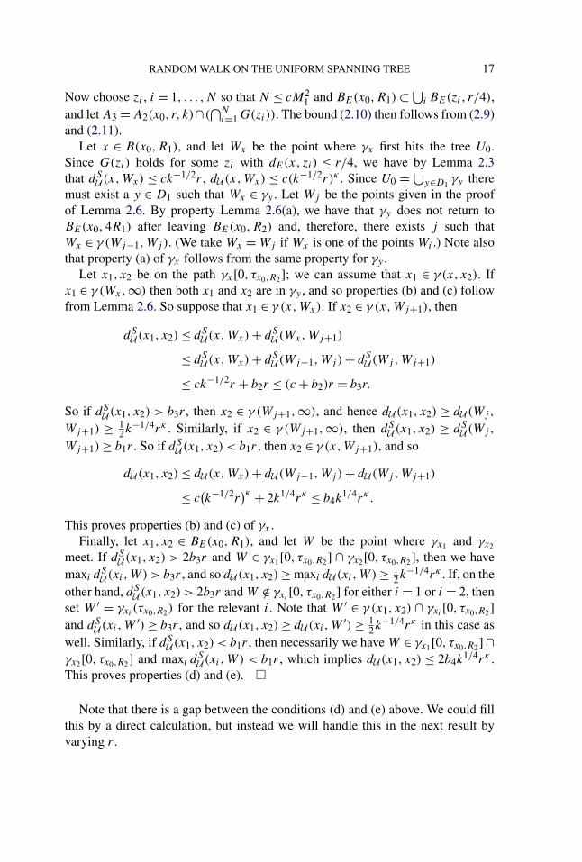
The second topic of this paper is the scaling limit of the simple random walk(SRW) on the two-dimensional UST. For a given realisation of the graph U , theSRW on U is the discrete time Markov process XU = ((Xn)n≥0, (P
Ux )x∈Z2) which
at each time step jumps from its current location to a uniformly chosen neighbourin U (considered as a graph); see Figure 1. For x ∈ Z2, the law P U
x is called thequenched law of the simple random walk on U started at x. Since 0 is always anelement of U , we can define the annealed or averaged law P as the semi-directproduct of the environment law P and the quenched law P U
0 by setting
P(·) :=∫
P U0 (·) dP.(1.5)
It is this measure for which we will deduce scaling behaviour.Techniques for deriving the scaling limits of random walks on the kinds of
trees generated by critical branching processes have previously been developedin [16, 20, 21]; see also [36], Chapter 7, for a survey. In the present work, weadapt these to prove a general result of the following form; see Theorem 6.1below for details and some additional technical conditions. If we have a se-quence of graph trees (Tn), n ≥ 1, each equipped with its intrinsic metric dTn ,a measure μTn , an embedding φTn : Tn → R2 and a distinguished root vertex ρn,for which there exist null sequences (an)n≥1, (bn)n≥1, (cn)n≥1 with bn = o(an)

8 M. T. BARLOW, D. A. CROYDON AND T. KUMAGAI
FIG. 1. The range of a realisation of the simple random walk on uniform spanning tree on a 60×60box (with wired boundary conditions), shown after 5000 and 50,000 steps. From most to least crossededges, colours blend from red to blue.
such that (Tn, andTn, bnμTn, cnφTn, ρTn) → (T , dT ,μT , φT , ρT ) in the space ofmeasured, rooted spatial trees, then the corresponding rescaled random walks(cnφTn(X
Tn
t/anbn))t≥0 converge in distribution. Further, the limiting process can be
written as (φT (XTt ))t≥0, where XT = ((XT
t )t≥0, (PTx )x∈T ) is the canonical Brow-
nian motion on (T , dT ,μT ), as constructed in [6], for example, cf. [32]. (We givea brief introduction to Brownian motion on measured real trees at the start of Sec-tion 6.)
Combining Theorems 1.1 and 6.1 we obtain the following theorem, which es-tablishes the existence of subsequential scaling limits for the annealed law of thesimple random walk on U . Given the volume estimates (1.3), the general results of[18] yield sub-diffusive transition density bounds for the limiting diffusion. Thesedemonstrate that, uniformly over bounded regions of space, the transition densityin question has at most logarithmic fluctuations from the leading order polynomialterms in both the on-diagonal and exponential off-diagonal decay parts. In Sec-tion 7, we also deduce pointwise on-diagonal estimates with only log-logarithmicfluctuations (cf. the discrete result of [11], Theorem 4.5(a)), as well as annealedon-diagonal polynomial bounds. We note the similarity between these results andthe transition density estimates for the Brownian continuum random tree givenin [19].
THEOREM 1.4. If (Pδi)i≥1 is a convergent sequence with limit P, then the
following statements hold:

RANDOM WALK ON THE UNIFORM SPANNING TREE 9
(a) The annealed law of (φT (XTt ))t≥0, where XT is Brownian motion on
(T , dT ,μT ) started from ρT , that is,
P(·) :=∫
P TρT ◦ φ−1
T (·) dP,(1.6)
is a well-defined probability measure on C(R+,R2).(b) If Pδ is defined to be the law of (δXU
δ−κdw t)t≥0 under P, where the walk
dimension dw of U is defined by
dw := 1 + df = 135 ,
then (Pδi)i≥1 converges to P.
(c) P-a.s., the process XT is recurrent and admits a jointly continuous tran-sition density (pT
t (x, y))x,y∈T ,t>0. Moreover, it P-a.s. holds that, for any R > 0,there exist random constants ci(T ) and t0(T ) ∈ (0,∞) and deterministic con-stants θ1, θ2, θ3, θ4 ∈ (0,∞) (not depending on R) such that
pTt (x, y) ≤ c1(T )t−df /dw�
(t−1)θ1
× exp{−c2(T )
(dT (x, y)dw
t
)1/(dw−1)
�(dT (x, y)/t
)−θ2
},
pTt (x, y) ≥ c3(T )t−df /dw�
(t−1)−θ3
× exp{−c4(T )
(dT (x, y)dw
t
)1/(dw−1)
�(dT (x, y)/t
)θ4
},
for all x, y ∈ BT (ρT ,R), t ∈ (0, t0(T )), where �(x) := 1 ∨ logx.
REMARK 1.5. If follows that for P-a.e. realisation of (T , dT ,μT , φT , ρT ),we have that
− limt→0
2 logpTt (x, x)
log t= 2df
1 + df
= 16
13for every x ∈ T .
Using the language of diffusions on fractals, this means that the spectral dimensionof the limiting tree is P-a.s. equal to 16/13, which is the same as for the discretemodel (see [11]).
The remainder of this article is organised as follows. In Section 2, we provesome key estimates for U , which enable us to compare distances in the Euclideanand intrinsic metrics on this set. These allow us to extend some of the volumeestimates of [11]. In Section 3, we introduce our topology for measured, rootedspatial trees, and in Section 4 we prove tightness in this topology for the rescaledtrees. The properties of limiting trees are studied in Section 5. Following this, weturn our attention to the simple random walk on U , establishing in Section 6 a gen-eral convergence result for simple random walks on measured, rooted spatial trees

10 M. T. BARLOW, D. A. CROYDON AND T. KUMAGAI
and applying this to the two-dimensional UST. In addition, we explain how thisconvergence result can be applied to branching random walks and trees withoutembeddings. In Section 7, we then derive the transition density estimates for thelimiting diffusion.
We write c or ci for constants in (0,∞); these will be universal and nonrandom,but may change in value from line to line. We use the notation ci(T ) for (random)constants which depend on the tree T .
2. UST estimates. In this section, we obtain estimates for the two-dimensional UST U , which improve those in [11]. Our arguments will dependheavily on Wilson’s algorithm, which gives the construction of U in terms ofLERW. In particular, we can construct U by first running an infinite loop-erasedrandom walk from 0 to ∞ (for details of this see [45]), and then, sequentially run-ning through vertices x ∈ Z2 \ {0}, adding a loop-erased random walk path fromx ∈ Z2 to the part of the tree already created. We remark that U is a one-endedtree; see [12].
We will consider three metrics on U , which we now introduce. We define dE tobe the Euclidean metric on Z2, and write BE(x, r) = {y : dE(x, y) ≤ r} for ballsin this metric. For x ∈ Z2, we let γ (x, y) be the unique path in U between x and y.We define the intrinsic (shortest path) metric dU by setting dU (x, y) := |γ (x, y)|,that is, the number of edges on the path γ (x, y), and write BU (x, r) for balls in thismetric. Finally, it will also be helpful to use a modification of a metric introducedby Schramm in [48], given by
dSU (x, y) := diam
(γ (x, y)
),(2.1)
where the right-hand side refers to the diameter of γ (x, y) in the metric dE .We begin by recalling the comparison between BU (0, r1/κ) and BE(0, r) and
the estimates on the size of |BU (0, r)| from [11].
THEOREM 2.1 (See [11], Theorems 1.1, 1.2). (a) There exist c1, c2 such thatfor every r ≥ 1 and λ ≥ 1,
P(BU
(0, λ−1rκ) �⊂ BE(0, r)
) ≤ c1e−c2λ
2/3,
P(BE(0, r) �⊂ BU
(0, λrκ)) ≤ c1λ
−1/5.
(b) There exist c1, c2 such that for every r ≥ 1 and λ ≥ 1,
P(∣∣BU (0, r)
∣∣ ≥ λrdf) ≤ c1e
−c2λ1/3
,
P(∣∣BU (0, r)
∣∣ ≤ λ−1rdf) ≤ c1e
−c2λ1/9
.
Since the law of U is translation invariant, the above result also holds forBU (x, r) for any x ∈ Zd . However, we wish to have these bounds (for suitable r, n)

RANDOM WALK ON THE UNIFORM SPANNING TREE 11
for every x ∈ BE(0, n); obtaining such uniform estimates is one of the main goalsof this section. If we use a simple union bound, as, for example, in [11], (4.47),we obtain an error estimate of the form n2 exp(−λc), which is only small whenλ (logn)1/c. To improve this, for a suitable δ = δ(λ) > 0 we choose a δ-coverD of BE(0, n) with |D| ≤ cδ−2. (Recall that a subset A of Z2 is called a λ-coverif every point of Z2 is within distance λ of a point of A.) We then obtain goodbehaviour of BU (x, r) for all x ∈ D, except on a set of probability |D| exp(−λc).Using a “filling in lemma” (see Lemma 2.3 below), together with some additionalbounds, we are able to extend this good behaviour to BU (y, r) for all y ∈ BE(0, n);see Proposition 2.10 below for a uniform version of part (b) in particular. An ex-ample of the kind of additional result that we need is that if dE(x, y) = 3r thenevery path in U between BE(x, r) and BE(y, r) is of length at least crκ , excepton a set of trees of small probability; note that [10], Theorem 1.2, shows that withhigh probability the unique infinite self avoiding path in U started from x takesat least crκ steps to escape a Euclidean ball of radius r , but again this does notreadily extend to a uniform bound and so further work is required.
We proceed by introducing some further notation and results from [11]. Letγx = γ (x,∞) be the unique infinite self avoiding path in U started at x; by Wil-son’s algorithm γx has the law of the loop-erased random walk from x to ∞. Writeγx[i] for the ith point on γx , and let τy,r = τy,r (γx) = min{i : γx[i] /∈ BE(y, r)}.Whenever we use notation such as γx[τy,r ], the exit time τy,r will always be forthe path γx . We define the segment of the path γx between its ith and j th points byγx[i, j ] = (γx[i], γx[i + 1], . . . , γx[j ]), and define γx[i,∞) in a similar fashion.For such paths, the following was established in [11].
LEMMA 2.2 (See [11], Lemma 2.4). There exists c1 such that for every r ≥ 1and k ≥ 2,
P(γx[τx,kr ,∞) ∩ BE(x, r) �= ∅
) ≤ c1k−1.
We next give the filling in lemma that we will use several times. This is a smallextension of [11], Proposition 3.2. Note that [10], Proposition 6.2, shows that thefunction G(r) considered in [11] is comparable with the function G2(r) appearingin (1.1).
LEMMA 2.3. There exist constants c1, c2 ∈ (0,∞) such that for each δ ≤ 1the following holds. Let r ≥ 1, and U0 be a fixed tree in Z2 with the property thatdE(x,U0) ≤ δr for each x ∈ BE(0, r). Let U be the random spanning tree in Z2
obtained by running Wilson’s algorithm with root U0 (i.e., starting from the treeU0). Then there exists an event G such that P(Gc) ≤ c1e
−c2δ−1/3
, and on G wehave that for all x ∈ BE(0, r/2),
dU (x,U0) ≤ (δ1/2r
)κ; dSU (x,U0) ≤ δ1/2r; γ (x,U0) ⊂ BE(0, r).

12 M. T. BARLOW, D. A. CROYDON AND T. KUMAGAI
PROOF. Except for the bound involving dSU this is proved in [11]. [Note that
the hypothesis there that U0 connects 0 to BE(0,2r)c is unnecessary.] The proofof the dS
U bound is similar. �
The following sequence of lemmas will improve the results in [11] on thecomparison of the metrics dU , dE and dS
U . Fix for now r, k ≥ 1 and x ∈ Z2,and choose points zj on γx so that z0 = x and zj = γx[sj ], where sj = min{i :dE(γx[i], {z0, . . . , zj−1}) ≥ r/k}. Let N = N(r, k) = max{j : sj ≤ τx,r (γx)}.Moreover, define a collection of disjoint balls Br,k = {Bj = BE(zj , r/3k), j =1, . . . ,N(r, k)}. These depend on the path γx , and when we need to recall this wewill write Br,k(γx). Let a = 1 + k−1/8, and set
F1(x, r, k) = {γx[τx,ar ,∞] hits fewer than k1/2 of B1, . . . ,BN(r,k)
}.
LEMMA 2.4. There exist constants c1, c2 ∈ (0,∞) such that, if r, k ≥ 1 andx ∈ Z2, then
P(F1(x, r, k)c
) ≤ c1e−c2k
1/8.
PROOF (see [11], Lemma 3.7). Write τs = τx,s(γx), and let b = ek1/8 ≥ 2.Then by Lemma 2.2,
P(γx[τbr ,∞] ∩ BE(x, r) �= ∅
) ≤ cb−1 = ce−k1/8.(2.2)
If γx[τar ,∞] hits more than k1/2 balls from the family Br,k(γx), then either γx hitsBE(0, r) after time τbr , or γx[τar , τbr ] hits more than k1/2 balls. Given (2.2), it istherefore sufficient to prove that
P(γx[τar , τbr ] hits more than k1/2 balls
) ≤ c1e−c2k
1/8.(2.3)
Let S be a simple random walk on Z2 started at x, L′ be the loop-erasure ofS[0, τx,4br(S)], and L′′ = L′[τx,ar (L
′), τx,br (L′)]. Then by [45], Corollary 4.5, in
order to prove (2.3), it is sufficient to prove that
P(L′′ hits more than k1/2 balls in Br,k
(L′)) ≤ c1e
−c2k1/8
.
Define stopping times for S by letting T0 = τx,ar (S) and for j ≥ 1, setting Rj =min{n ≥ Tj−1 : Sn ∈ BE(x, r)} and Tj = min{n ≥ Rj : Sn /∈ BE(x, ar)}. Note thatthe balls in Br,k(L
′) can only be hit by S in the intervals [Rj ,Tj ] for j ≥ 1.Let M = min{j : Rj ≥ τx,4br (S)}. Then, by the result of [39], Exercise 1.6.8,P(M = j + 1|M > j) ≥ c(log(ar) − log r)/(log(4br) − log r) ≥ ck−2/8. Hence,P(M ≥ k3/8) ≤ c1 exp(−c2k
1/8). Now, for each j ≥ 1, let Lj be the loop-erasureof S[0, Tj ], αj be the first exit by Lj from BE(x, ar), and βj be the numberof steps in Lj . If L′′ hits more than k1/2 balls in Br,k(L
′), then there must existsome j ≤ M such that Lj [αj ,βj ] hits more than k1/2 of the balls in the collec-tion Br,k(Lj ). Hence, if M ≤ k3/8 and L′′ hits more than k1/2 balls in Br,k(L
′),

RANDOM WALK ON THE UNIFORM SPANNING TREE 13
FIG. 2. A sample of A1(x, r, k) in Lemma 2.5.
then S must hit more than k1/8 balls in Br,k(Lj ) in one of the intervals [Rj ,Tj ],without hitting the path Lj [0, αj ]. However, by Beurling’s estimate (see [39],Lemma 2.5.3, e.g.), the probability of this event is less than c1 exp(−c2k
1/8). Com-bining these estimates completes the proof. �
Our next lemma shows that if D0 is δr-cover of BE(x,2r), then with highprobability we can find points Yx,r and Wx,r which are close to the boundary ofBE(x, r) and to each other, and such that Yx,r ∈ D0 and Wx,r ∈ γx ∩BE(x, r). (SeeFigure 2.) In the proof, we refer to the event F2(x, r, k) = {8k−1/4rκ ≤ τx,r (γx) ≤k1/4rκ}. From [10], Theorems 5.8, 6.1, we have
P(F2(x, r, k)c
) ≤ c1 exp(−c2k
1/6).(2.4)
LEMMA 2.5. Let r ≥ 1, k ≥ 2, x ∈ Z2, and D0 ⊂ Z2 satisfy BE(x,2r) ⊂⋃y∈D0
BE(y, r/18k). Then there exists an event A1 = A1(x, r, k), defined in (2.8)below, which satisfies
P(Ac
1) ≤ e−k1/8
,(2.5)
and on A1(x, r, k) there exists T ≤ τx,r (γx) such that, writing Wx,r = γx(T ):
(a) k−1/4rκ ≤ T ≤ k1/4rκ ;(b) a−2r ≤ dE(x,Wx,r ) ≤ r ;(c) there exists Yx,r ∈ D0 such that dE(Yx,r ,Wx,r) ≤ r/3k, dS
U (Yx,r ,Wx,r ) ≤2r/3k and also dU (Yx,r ,Wx,r ) ≤ c1(r/k)κ .

14 M. T. BARLOW, D. A. CROYDON AND T. KUMAGAI
PROOF. Fix k ≥ 1 and recall that a = 1 + k−1/8. Suppose that the event
F1(x, r/a, k) ∩ F2(x, r/a2, k
) ∩ F2(x, r, k)(2.6)
occurs. Write τs = τx,s(γx), T1 = τr/a2 , and T2 = τr/a . Let J0 = J0(ω) be the set ofj such that zj ∈ γx[T1, T2] and BE(zj , r/3ak) ⊂ BE(x, r/a) \ BE(x, r/a2). Then|J0| ≥ ck7/8. Since F1(x, r/a, k) holds, at most k1/2 of the balls (BE(zj , r/3ak),
j ∈ J0) are hit by γx[τr ,∞]. So if J = J (ω) is the set of j ∈ J0 such thatBE(zj , r/3ak) ∩ γx[τr ,∞] = ∅, then |J | ≥ k7/8 − k1/2 ≥ ck3/4. For each j ∈ J ,we can find a point yj ∈ D0 with dE(yj , zj ) ≤ r/18k. Hence, BE(yj , r/18k) ∩γx[T1, T2] �=∅, while BE(yj , r/9k)∩γx[τr ,∞] = ∅. Note that BE(yj , r/9k) mayhowever intersect the path γx in the interval [T2, τr ].
For the remainder of the proof, it will be helpful to regard γx as a fixed deter-ministic path which satisfies the conditions in (2.6). For each j ∈ J , let Xj be aSRW started at yj and run until it hits γx , and let Lj be the loop-erasure of Xj .Let
Hj = {Xj hits γx before it exits BE(zj , r/3ak),
∣∣Lj∣∣ ≤ c0(r/3k)κ
}.
By [11], Theorem 2.2, we have [taking D = Z2 \γx and D′ = D∩BE(zj , r/3ak)],
P(∣∣Lj ∩ BE(zj , r/3ak)
∣∣ > λ(r/k)κ) ≤ c1 exp(−c2λ).
So, by Beurling’s estimate (see [39], Lemma 2.5.3, e.g.), we can choose c0 so thatthere exists p > 0 such that P(Hj ) ≥ p.
Recall now the implementation of Wilson’s algorithm using “stacks” (see [49]).For each j , assume we have stack variables ξx,i for x ∈ BE(zj , r/3ak). We usethese to make a random walk path Xj started at yj and run either it hits γx or leavesBE(zj , r/3ak). Thus, the event Hj is measurable with respect to σ(ξx,i , i ≥ 1, x ∈BE(zj , r/3ak)). We now consider the yj one at a time, and continue until eitherwe obtain a success, or we have tried k3/4 of the points yj . Since these events areindependent, if H is the event that we obtain a success, then
P(Hc) ≤ (1 − p)k
3/4 ≤ c1 exp(−c2k
3/4).(2.7)
If H occurs, with a success for yj , set Y = Yx,r = yj , let W = Wx,r be the pointwhere Xj hits γx , and let T be such that γx(T ) = W . We take
A1 = A1(x, r, k) = H ∩ F1(x, r/a, k) ∩ F2(x, r/a2, k
) ∩ F2(x, r, k).(2.8)
By Lemma 2.4, (2.4) and (2.7), we have the upper bound (2.5) on P(Ac1).
Finally, suppose that A1(x, r, k) occurs. By construction, we have dE(Y,W) ≤r/3k, and since the path Xj lies inside BE(zj , r/3k) we also have dS
U (Y,W) ≤2r/3k. The definition of the event Hj gives that dU (Y,W) ≤ c(r/k)κ . Since Xj
hits γx inside BE(zj , r/3ak), we must have W ∈ BE(x, r) \ BE(x, a−2r). More-over, because j ∈ J , T ≤ τr(γx), so since F2(x, k, r) holds we have T ≤ k1/4rκ .

RANDOM WALK ON THE UNIFORM SPANNING TREE 15
Since BE(zj , r/3ak) ∩ BE(x, r/a2) = ∅, we must also have T ≥ τr/a2 , and soT ≥ 8k−1/4(r/a2)κ ≥ k−1/4rκ . �
The next lemma allows us to compare dSU and dU on a large family of paths in a
ball.
LEMMA 2.6. Let r ≥ 1, k ≥ 8, and x ∈ Z2. Set M1 = ek1/8/27, M2 = ek1/8/3,Ri = rMi , and let D0 ⊂ BE(x,2R2) satisfy |D0| ≤ ck2M2
2 , |D0 ∩ BE(x,2R1)| ≤ck2M2
1 , BE(x,2R2) ⊂ ⋃y∈D0
BE(y, r/18k). Write D1 = D0 ∩ BE(x,2R1). Thenthere exist constants b1, b2 and an event A2 = A2(x, r, k) with
P(Ac
2) ≤ c exp
(−k1/8/4),(2.9)
such that on A2 the following holds for every y ∈ D1:
(a) γy[τx,R2,∞] ∩ BE(x,4R1) =∅;(b) if x1, x2 ∈ γy[0, τx,R2] and dS
U (x1, x2) > b2r , then dU (x1, x2) ≥ 12k−1/4rκ ;
(c) if x1, x2 ∈ γy[0, τx,R2] and dSU (x1, x2) < b1r , then dU (x1, x2) ≤ 2k1/4rκ .
PROOF. For y ∈ D1, let F3(y, r, k) = {γy[τx,R2,∞] ∩ BE(x,4R1) = ∅}. ByLemma 2.2, we have P(F c
3 ) ≤ cM1/M2. Now set
A2 =( ⋂
y∈D0
A1(y, r, k)
)∩
( ⋂y∈D1
F3(y, r, k)
),
where A1(y, r, k) is the event defined by (2.8). From (2.5), we note that
P(Ac
2) ≤ ck2M2
2e−k1/8 + cM21k2M1M
−12 ≤ c exp
(−k1/8/4).
Now suppose that A2 holds, and let y ∈ D1. It is immediate that (a) holds.Write W0 = Y0 = y, and let Y1 = YY0,r and W1 = WY0,r be the points given bythe event A1(Y0, r, k). Similarly write Yj+1 and Wj+1 for the points given by theevent A1(Yj , k, r) for j ≥ 1, and continue until we have for some N = Ny thatWN /∈ BE(x,3R2/2). Note that both dS
U and dU are monotone on the path γy ,in the sense that if x1, x2 ∈ γy and x3 ∈ γ (x1, x2) then for ρ = dS
U or ρ = dUthen ρ(x1, x3) ≤ ρ(x1, x2). This is immediate for dU and easily proved from thedefinition of dS
U .The construction of the (Yj ,Wj ) gives that
r
a2 ≤ dSU (Yj ,Wj+1) ≤ r, dS
U (Yj ,Wj ) ≤ 2r
k,
k−1/4rκ ≤ dU (Yj ,Wj+1) ≤ k1/4rκ, dU (Yj ,Wj ) ≤ c(r/k)κ .

16 M. T. BARLOW, D. A. CROYDON AND T. KUMAGAI
Thus, we have
dSU (Wj ,Wj+1) ≤ dS
U (Wj ,Yj ) + dSU (Yj ,Wj+1) ≤ 2r
k+ r = 1
2b2r,
dSU (Wj ,Wj+1) ≥ dS
U (Yj ,Wj+1) − dSU (Wj ,Yj ) ≥ r/a2 − 2r
k= b1r.
Here, we have used the equations above to define b1 and b2. Similarly, we have
dU (Wj ,Wj+1) ≤ dU (Yj ,Wj+1) ≤ k1/4rκ,
dU (Wj ,Wj+1) ≥ dU (Yj ,Wj+1) − dU (Yj ,Wj ) ≥ k−1/4rκ − c(r/k)κ ≥ 12k−1/4rκ .
Let x1, x2 ∈ γy[0, τx,3R2/2]. We can assume that x1 ∈ γ (y, x2). Let j =min{i : Wi ∈ γ (x1,∞)}. If x2 ∈ γ (x1,Wj+1), then dS
U (x1, x2) ≤ dSU (Wj−1,Wj ) +
dSU (Wj ,Wj+1) ≤ b2r . So if dS
U (x1, x2) > b2r , then both Wj and Wj+1 are onthe path γ (x1, x2), and so dU (x1, x2) ≥ 1
2k−1/4rκ , proving (b). Similarly, if bothWj and Wj+1 are on the path γ (x1, x2), then we have dS
U (x1, x2) ≥ b1r . So ifdSU (x1, x2) < b1r , then Wj+1 ∈ γ (x2,∞), and hence dU (x1, x2) ≤ 2k1/4rκ . �
We now extend this result to all paths γx in a ball.
LEMMA 2.7. Let r ≥ 1, k ≥ 8, x0 ∈ Z2, Mi,Ri , and b1, b2 be as inLemma 2.6. Then there exist constants b3, b4 (depending on k) and an eventA3 = A3(x0, r, k) with
P(Ac
3) ≤ c1 exp
(−c2k1/8)
,(2.10)
such that on A3 the following holds for every x ∈ BE(x0,R1):
(a) γx[τx0,R2,∞] ∩ BE(x0,4R1) = ∅;(b) If x1, x2 ∈ γx[0, τx0,R2] and dS
U (x1, x2) > b3r , then dU (x1, x2) ≥ 12k−1/4rκ ;
(c) If x1, x2 ∈ γx[0, τx0,R2] and dSU (x1, x2) < b1r , then dU (x1, x2) ≤ b4k
1/4rκ ;(d) If x1, x2 ∈ BE(x0,R1) and dS
U (x1, x2) > 2b3r , then dU (x1, x2) ≥ 12k−1/4rκ ;
(e) If x1, x2 ∈ BE(x0,R1) and dSU (x1, x2) < b1r , then dU (x1, x2) ≤ 2b4k
1/4rκ .
PROOF. We begin by choosing a set D0 which satisfies the conditions ofLemma 2.6. Let A2(x0, r, k) be the event defined in that lemma, and let U0 be therandom tree obtained by applying Wilson’s algorithm with initial points in D1 =D0 ∩ B(x0,2R1). Let z ∈ BE(x0,R1). We now apply the filling in Lemma 2.3 toBE(z, r) taking δ = 1/18k. Let G(z) be the “good” event given by the lemma; wehave
P(G(z)c
) ≤ c exp(−ck1/3)
.(2.11)
RANDOM WALK ON THE UNIFORM SPANNING TREE 17
Now choose zi , i = 1, . . . ,N so that N ≤ cM21 and BE(x0,R1) ⊂ ⋃
i BE(zi, r/4),and let A3 = A2(x0, r, k)∩(
⋂Ni=1 G(zi)). The bound (2.10) then follows from (2.9)
and (2.11).Let x ∈ B(x0,R1), and let Wx be the point where γx first hits the tree U0.
Since G(zi) holds for some zi with dE(x, zi) ≤ r/4, we have by Lemma 2.3that dS
U (x,Wx) ≤ ck−1/2r , dU (x,Wx) ≤ c(k−1/2r)κ . Since U0 = ⋃y∈D1
γy theremust exist a y ∈ D1 such that Wx ∈ γy . Let Wj be the points given in the proofof Lemma 2.6. By property Lemma 2.6(a), we have that γy does not return toBE(x0,4R1) after leaving BE(x0,R2) and, therefore, there exists j such thatWx ∈ γ (Wj−1,Wj ). (We take Wx = Wj if Wx is one of the points Wi .) Note alsothat property (a) of γx follows from the same property for γy .
Let x1, x2 be on the path γx[0, τx0,R2]; we can assume that x1 ∈ γ (x, x2). Ifx1 ∈ γ (Wx,∞) then both x1 and x2 are in γy , and so properties (b) and (c) followfrom Lemma 2.6. So suppose that x1 ∈ γ (x,Wx). If x2 ∈ γ (x,Wj+1), then
dSU (x1, x2) ≤ dS
U (x,Wx) + dSU (Wx,Wj+1)
≤ dSU (x,Wx) + dS
U (Wj−1,Wj ) + dSU (Wj ,Wj+1)
≤ ck−1/2r + b2r ≤ (c + b2)r = b3r.
So if dSU (x1, x2) > b3r , then x2 ∈ γ (Wj+1,∞), and hence dU (x1, x2) ≥ dU (Wj ,
Wj+1) ≥ 12k−1/4rκ . Similarly, if x2 ∈ γ (Wj+1,∞), then dS
U (x1, x2) ≥ dSU (Wj ,
Wj+1) ≥ b1r . So if dSU (x1, x2) < b1r , then x2 ∈ γ (x,Wj+1), and so
dU (x1, x2) ≤ dU (x,Wx) + dU (Wj−1,Wj ) + dU (Wj ,Wj+1)
≤ c(k−1/2r
)κ + 2k1/4rκ ≤ b4k1/4rκ .
This proves properties (b) and (c) of γx .Finally, let x1, x2 ∈ BE(x0,R1), and let W be the point where γx1 and γx2
meet. If dSU (x1, x2) > 2b3r and W ∈ γx1[0, τx0,R2] ∩ γx2[0, τx0,R2], then we have
maxi dSU (xi,W) > b3r , and so dU (x1, x2) ≥ maxi dU (xi,W) ≥ 1
2k−1/4rκ . If, on theother hand, dS
U (x1, x2) > 2b3r and W /∈ γxi[0, τx0,R2] for either i = 1 or i = 2, then
set W ′ = γxi(τx0,R2) for the relevant i. Note that W ′ ∈ γ (x1, x2) ∩ γxi
[0, τx0,R2]and dS
U (xi,W′) ≥ b3r , and so dU (x1, x2) ≥ dU (xi,W
′) ≥ 12k−1/4rκ in this case as
well. Similarly, if dSU (x1, x2) < b1r , then necessarily we have W ∈ γx1[0, τx0,R2] ∩
γx2[0, τx0,R2] and maxi dSU (xi,W) < b1r , which implies dU (x1, x2) ≤ 2b4k
1/4rκ .This proves properties (d) and (e). �
Note that there is a gap between the conditions (d) and (e) above. We could fillthis by a direct calculation, but instead we will handle this in the next result byvarying r .

18 M. T. BARLOW, D. A. CROYDON AND T. KUMAGAI
PROPOSITION 2.8. Let r ≥ 1, λ ≥ λ0 (where λ0 is a large, finite constant),x0 ∈ Z2, and R = rec1λ
1/2. There exists an event A4 with P(Ac
4) ≤ c exp(−c2λ1/2)
such that on A4, for all x, y ∈ BE(x0,R),
λ−1dSU (x, y)κ ≤ dU (x, y) ≤ λdS
U (x, y)κ if r ≤ dSU (x, y) ≤ R,
dU (x, y) ≤ λrκ if dSU (x, y) ≤ r,(2.12)
dU (x, y) ≥ λ−1Rκ if dSU (x, y) ≥ R.
PROOF. Choose k = cλ4, let m be such that 2m−1 < exp(k1/8/27) ≤ 2m,and define A4 = ⋂m
i=0 A3(x0,2ir, k). Then P(Ac4) ≤ exp(−ck1/8) ≤ exp(−c′λ1/2).
Now let x, y ∈ BE(x0,R), and suppose r ′ = dSU (x, y) ≤ R. Then choosing the
largest i ∈ {0,1, . . . ,m} so that r ′ ≥ 2b32ir , we have dU (x1, x2) ≥ cλ−1(2ir)κ ≥cλ−1(r ′)κ . Similarly, we have dU (x1, x2) ≤ cλ(r ′)κ . Replacing cλ by λ thisgives (2.12), and the other two inequalities follow. �
One consequence of the above proposition is the following approximation re-sult, which shows that if a set of points is an r/18k2-cover in the Euclidean metric,then it is also a cover with respect to the metrics dS
U and dU .
PROPOSITION 2.9. Let r ≥ k ≥ 1. Define R1 := rek1/32, R2 := rek1/16
, andsuppose D2 ⊆ Z2 satisfies
BE(0,6R2) ⊆ ⋃x∈D2
BE
(x, r/18k2)
.(2.13)
Then there exists an event A5 = A5(r, k) such that P(Ac5) ≤ c1e
−c2k1/16
and on A5the following holds:
maxx∈BE(0,R1)
dSU (x,D2) ≤ 2r
k,(2.14)
maxx∈BE(0,R1)
dU (x,D2) ≤ 4rκ
k1/4 .(2.15)
PROOF. First, choose a subset D′2 ⊆ D2 such that (2.13) holds when D2 is
replaced by D′2 and also |D′
2| ≤ ck4e2k1/16. Set A′(r, k) := ⋂
x∈D′2A1(x, r/k, k),
where A1 is defined in the statement of Lemma 2.5. From that result, we knowthat
P(A′c) ≤ ck4e2k1/16
P(A1(0, r/k, k)
) ≤ ce−ck1/8.(2.16)
Moreover, if A′ holds, then for x ∈ BE(0,2R1) ∩ D′2 we can define (Wj ,Yj )
Nj=0
similarly to the proof of Lemma 2.6. In particular, set W0 = Y0 = x, and let Wj,Yj

RANDOM WALK ON THE UNIFORM SPANNING TREE 19
be given by the event A1(Yj−1, r/k, k), up to j = N := inf{m : dE(x,Wm) >
2R2}. By construction, it follows that
maxz∈γx(0,τx,R2 )
dSU (z,D2) ≤ max
j=1,...,NdSU (Wj−1,Wj )
(2.17)≤ max
j=1,...,NdSU (Yj−1,Wj ) ≤ r
k.
Next, choose D′′2 ⊆ D′
2 ∩BE(0,2R1) such that BE(0,R1) ⊆ ⋃x∈D′′
2BE(x, r/18k2)
and |D′′2 | ≤ ck4e2k1/32
. Set A′′(r, k) := A′(r, k) ∩ (⋂
x∈D′′2B(x, r, k)), where
B(x, r, k) := {γx(τx,R2,∞) ∩ BE(0,2R1) = ∅}. By applying Lemma 2.2 in con-junction with (2.16), we obtain
P(A′′c) ≤ ce−ck1/8 + ck4e2k1/32
P(γ0(τ0,R2,∞) ∩ BE(0,4R1) �= ∅
) ≤ c1e−c2k
1/16.
Define U0 to be the subtree of U spanned by D′′2 and suppose A′′ holds. If
x ∈ U0 ∩ BE(0,2R1), then it must be the case that x ∈ γy(0, τy,R2) for somey ∈ D′′
2 . Hence, by (2.17), it holds that maxx∈U0∩BE(0,2R1) dSU (x,D2) ≤ r/k. Now,
by applying Lemma 2.3 with root U0, it is possible to deduce
P(
maxx∈BE(0,R1)
dSU (x,U0) >
r
k
)≤ Ce−cek1/32
.
So, if A′′′ is defined to be the event that both A′′ and maxx∈BE(0,R1) dSU (x,U0) ≤
r/k hold, then we have P(A′′′c) ≤ c1e−c2k
1/16and also (2.14) holds on A′′′.
To complete the proof, we will use Proposition 2.8 with (x0, r, λ) given by(0,2r/k, k) to compare the relevant distances. Since R = 2rk−1ec1k
1/2 ≥ 2R1 forlarge k, we find that with probability exceeding 1 − ce−c2k
1/2it is the case that
maxx,y∈BE(0,2R1):dSU (x,y)≤2r/k
dU (x, y) ≤ k
(2r
k
)κ
≤ 4rκ
k1/4 .
Note that if A′′′ and the above inequality both hold, then so does (2.15). Hence,in conjunction with the conclusion of the previous paragraph, this completes theproof. �
We can now improve the volume estimates of [11]. Recall from (1.2) that df =2/κ = 8/5, and define, for λ,n ≥ 1,
A(λ,n) := {ω : λ−1Rdf ≤ ∣∣BU (x,R)
∣∣ ≤ λRdf
for all x ∈ BE(0, n),R ∈ [e−λ1/40
nκ,nκ]}.
The following result extends a fundamental estimate of [11]; the key improvementis that the upper bound does not depend on n (once n is suitably large). Althoughwe do not need to do so here, we note that the same approach can also be used toobtain a similar improvement of the resistance estimates in [11].

20 M. T. BARLOW, D. A. CROYDON AND T. KUMAGAI
PROPOSITION 2.10. There exist constants c1, c2 ∈ (0,∞) such that
P(A(λ,n)c
) ≤ c1 exp(−c2λ
1/80)for all n ≥ eλ1/16
.
PROOF. Let k = λ, r = ne−λ1/32, and let R1 = n, R2 = rek1/6
and D2 be asin Proposition 2.9, with |D2| ≤ ck4e2k1/16
. Set m0 := inf{m : km ≥ ek1/32}. LetA5(r, k) be the event given in the statement of Proposition 2.9, and
E(r, k) := ⋂x∈D2
m0+1⋂m=1
{k−1(
rkm)κ ≤ ∣∣BU(x,
(rkm)κ)∣∣ ≤ k
(rkm)κ}
.
A simple union bound allows us to deduce from Theorem 2.1(b) that
P(E(r, k)c
) ≤ Ck4e2k1/16k1/32ce−k1/9 ≤ Ce−ck1/9
.
Consequently, we have P(E(r, k)c ∪ A5(r, k)c) ≤ c exp(−cλ1/16).Suppose that E(r, k) ∩ A5(r, k) holds. Let x ∈ BE(0, n), and s ∈ [rk3, n].
Choose m ∈ {3, . . . ,m0 + 1} such that s ∈ [rkm, rkm+1). Since A5(r, k) holds,there exists y ∈ D2 with dU (x, y) ≤ 4rκ/k1/4. Hence,∣∣BU
(x, sκ)∣∣ ≤ ∣∣BU
(y,
(rkm+1)κ + 4rκ/k1/4)∣∣ ≤ ∣∣BU
(y,
(rkm+2)κ)∣∣ ≤ k
(rkm+2)2
≤ k5s2.
Similarly, |BU (x, sκ)| ≥ k−5s2. Since (rk3)κ ≤ nκ exp(−λ1/40) it follows thatE(r, k) ∩ A5(r, k) ⊂ A(λ5, n), which completes the proof of the proposition. �
From this, we can prove the following distributional measure bounds, whichwill be used in the proof of Theorem 1.3(b)(ii).
COROLLARY 2.11. Given R > 0, there exist constants c1, . . . , c7 ∈ (0,∞)
(depending on R) such that for every r ∈ (0, c7),
lim supδ→0
P(δ2 min
x∈BE(0,δ−1R)μU
(BU
(x, δ−κr
)) ≤ c1rdf
(log r−1)−80
)(2.18)
≤ c2rc3,
lim supδ→0
P(δ2 max
x∈BE(0,δ−1R)μU
(BU
(x, δ−κr
)) ≥ c4rdf
(log r−1)80
)(2.19)
≤ c5rc6 .
PROOF. We just prove (2.19); the proof of (2.18) is similar. Fix R ≥ 1, andsuppose r ∈ (0,1), δ ∈ (0,1). Define n := δ−1R and λ := (log(Rκ/r))80. Sinceδ−κr ∈ [e−λ1/40
nκ,nκ ], we have that, on A(λ,n),
minx∈BE(0,δ−1R)
μU(BU
(x, δ−κr
)) ≥ λ−1δ−2rdf ≥ c1δ−2rdf
(log r−1)−80
.

RANDOM WALK ON THE UNIFORM SPANNING TREE 21
Hence, by Proposition 2.10, the left-hand side of (2.19) is bounded above byCe−cλ1/80
. �
Let NU (r, s) the minimum number of dU -balls of radius s required to coverBU (0, r). Another consequence of Proposition 2.10 is the following bound onNU (r, r/λ).
LEMMA 2.12. There exist constants c1, c2, c3, λ0 ∈ (0,∞) such that, for r ≥eκ(logλ)41/16
and λ ≥ λ0,
P(NU (r, r/λ) ≥ c1(logλ)107λdf
) ≤ c2e−c3(logλ)41/80
.
PROOF. Let θ ≥ 1 be such that 2λ ≤ θ−1 exp(θ1/40). By Theorem 2.1(a), wehave that
P(BU (0, r) �⊂ BE
(0, θ1/κr1/κ)) ≤ e−cθ2/3
.
Now it is straightforward to check that one can cover BU (0, r) by balls BU (zi, r/λ),i = 1, . . . ,M , such that BU (zi, r/2λ) are disjoint and zi ∈ BU (0, r). Moreover, itis necessarily the case that M ≥ NU (r, r/λ). Setting nκ = θr , if A(θ, n) holdsand BU (0, r) ⊂ BE(0, n) then we have |BU (0, r)| ≤ (θr)df and |BU (zi, r/2λ)| ≥cθ−1(r/λ)df for each i. Thus, we deduce from Proposition 2.10 that
P(NU (r, r/λ) ≥ cθ1+df λdf
) ≤ c exp(−cθ1/80)
.(2.20)
Taking θ = (logλ)41 completes the proof. �
REMARK 2.13. Taking θ = λ in (2.20) gives the bound, for r ≥ eκλ1/16and λ
large,
P(NU (r, r/λ) ≥ cλ1+2df
) ≤ c exp(−cλ1/80)
.
3. Topology for UST scaling limit. In this section, we introduce the topologyon measured, rooted spatial trees for which we prove tightness for the law of therescaled UST. This topology is finer than that considered in [2, 48], since it incor-porates the full convergence of real trees embedded into Euclidean space, ratherthan merely the shape of subsets spanning a finite number of vertices. This pointwill be important when it comes to the proof of Theorem 1.4.
We define T to be the collection of quintuplets of the form
T = (T , dT ,μT , φT , ρT ),
where: (T , dT ) is a complete and locally compact real tree (see [44], Defini-tion 1.1, e.g.); μT is a locally finite Borel measure on (T , dT ); φT is a con-tinuous map from (T , dT ) into a separable metric space (M,dM); and ρT is adistinguished vertex in T . [Usually the image space (M,dM) we consider is R2

22 M. T. BARLOW, D. A. CROYDON AND T. KUMAGAI
equipped with the Euclidean distance, though we will also consider other imagespaces at certain places in our arguments.] We call such a quintuplet a measured,rooted, spatial tree. Let Tc be the subset of T for which (T , dT ) is compact. Wewill say that two elements of T, T and T ′ say, are equivalent if there exists anisometry π : (T , dT ) → (T ′, d ′
T ) for which μT ◦ π−1 = μ′T , φT = φ′
T ◦ π andalso π(ρT ) = ρ′
T .In order to introduce a topology on T, we will start by defining a topology on Tc.
In particular, for two elements of Tc, we set �c(T ,T ′) to be equal to
infZ,ψ,ψ ′,C:(ρT ,ρ′
T )∈C
{dZP
(μT ◦ ψ−1,μ′
T ◦ ψ ′−1)
(3.1)+ sup
(x,x′)∈C(dZ
(ψ(x),ψ ′(x′)) + dM
(φT (x),φ′
T(x′)))},
where the infimum is taken over all metric spaces Z = (Z, dZ), isometric em-beddings ψ : (T , dT ) → Z, ψ ′ : (T ′, d ′
T ) → Z, and correspondences C betweenT and T ′, and we define dZ
P to be the Prohorov distance between finite Borelmeasures on Z. Note that, by a correspondence C between T and T ′, we mean asubset of T × T ′ such that for every x ∈ T there exists at least one x′ ∈ T ′ suchthat (x, x′) ∈ C and conversely for every x′ ∈ T ′ there exists at least one x ∈ Tsuch that (x, x′) ∈ C.
PROPOSITION 3.1. The function �c defines a metric on the equivalenceclasses of Tc. Moreover, the resulting metric space is separable.
PROOF. The proof of this result is almost identical to that of [22], Lemma 2.1,taking, in the notation of that paper, I = {1} and q1(x, y) := φT (x). The mainchange is that when considering a correspondence between T and T ′, one has torequire that the pair of roots (ρT , ρ′
T ) is included, and, when selecting the pointsxi , x′
i as in [22], one should take x1 = ρT and x′1 = ρ′
T . A second change is thatin the proof of separability, rather than approximating by metric spaces with afinite number of vertices, one should approximate by real trees formed of a finitenumber of line segments; however, making these changes is routine and we omitthe details. �
REMARK 3.2. Even if (M,dM) is assumed to be complete, the space of equiv-alence classes of Tc is not complete with respect to the metric �c in general.Indeed, suppose (M,dM) = (R2, d
(2)E ) and consider ([0,1], d(1)
E ,L, f,0) ∈ Tc,
where d(d)E is the d-dimensional Euclidean distance, L is Lebesgue measure on
[0,1], and f : [0,1] → R2 is any continuous nonconstant function. If we replaced
(1)E by εd
(1)E , then the sequence of elements in Tc that we obtain is Cauchy as
ε → 0, but does not have a limit in Tc. One way to ensure completeness would be

RANDOM WALK ON THE UNIFORM SPANNING TREE 23
to restrict to a subset of Tc for which the functions φT satisfy an equi-continuitycondition.
To extend �c to a metric on the equivalence classes of T, we considerbounded restrictions of elements of T (cf. [1]). Thus, for T ∈ T, let T (r) =(T (r), d
(r)T ,μ
(r)T , φ
(r)T , ρ
(r)T ) be obtained by taking: T (r) to be the closed ball in
(T , dT ) of radius r centred at ρT ; d(r)T μ
(r)T and φ
(r)T to be the restriction of dT ,
μT and φT , respectively, to T (r), and ρ(r)T to be equal to ρT . As in [1], the fact
that (T , dT ) is a real tree, and therefore a length space, means we can apply theHopf–Rinow theorem (which implies that all closed, bounded subsets of a com-plete and locally compact length space are compact) to establish that T (r) is anelement of Tc. Furthermore, as in [1], Lemma 2.8, we can check the regularity ofthis restriction with respect to the metric �c.
LEMMA 3.3. For any two elements of T, T and T ′, the function r �→�c(T (r),T ′(r)) is cadlag.
PROOF. By considering the natural embedding of T (r) into T (r+ε), along withthe correspondence consisting of pairs (x, x′) such that x is the closest point inT (r) to x′ ∈ T (r+ε), we have, as in [1], Lemma 5.2, that
�c
(T (r),T (r+ε)) ≤ μT
(T (r+ε) \ T (r)) + ε + sup
x,x′∈T (r+ε):dT (x,x′)≤ε
dM
(φT (x),φT
(x′));
given this, the proof is a straightforward adaption of the proof of [1], Lemma 2.8.�
This result allows us to well define a function � on T2 by setting
�(T ,T ′) :=
∫ ∞0
e−r(1 ∧ �c
(T (r),T ′(r)))dr.(3.2)
PROPOSITION 3.4. The function � defines a metric on the equivalence classesof T. Moreover, the resulting metric space is separable.
PROOF. Again, the proof is similar to the corresponding result in [1]. Posi-tivity, finiteness and symmetry of � are clear. Moreover, the triangle inequality iseasy to check from the definition and the fact that the triangle inequality holds for�c. So, to establish that � is a metric, it remains to prove positive definiteness.To this end, suppose that T and T ′ are such that the expression at (3.2) is equal tozero. From Lemma 3.3, it follows that �c(T (r),T ′(r)) = 0 for every r > 0. Conse-quently, for each r , there exists an isometry πr : (T (r), d
(r)T ) → (T ′(r), d ′(r)
T ) such
that μ(r)T ◦π−1
r = μ′(r)T , φ
(r)T = φ
′(r)T ◦πr and also πr(ρ
(r)T ) = ρ
′(r)T . For n, k ≥ 1, let

24 M. T. BARLOW, D. A. CROYDON AND T. KUMAGAI
(xn,ki )
N(n,k)i=1 be a finite k−1-cover of T (n) containing the root ρT (such a collection
exists as a result of the compactness of T (n)). Since πr is an isometry, we havethat (πm(x
n,ki ))m≥n is a bounded sequence for each n, k ≥ 1 and 1 ≤ i ≤ N(n, k),
and so has a convergent subsequence. By a diagonal procedure, one can thus finda subsequence (mj )j≥1 such that π(x
n,ki ) = limj→∞ πmj
(xn,ki ) exists for every
n, k ≥ 1 and 1 ≤ i ≤ N(n, k). From this construction, we obtain that π is distance-preserving on {xn,k
i : n, k ≥ 1,1 ≤ i ≤ N(n, k)} and, since the latter set is dense inT , we can extend it to a distance-preserving map on T . Clearly, by reversing theroles of T and T ′, it is also possible to find a distance-preserving map from T ′to T . Hence, π must be an isometry. Moreover, it is clear that this map is root-preserving, that is, π(ρT ) = ρ′
T . To check that it is measure-preserving, that is,μT ◦ π−1 = μ′
T , one can follow an identical argument to that applied in the proof
of [1], Proposition 5.3, based on considering approximations to the measures μ(n)T
and μ′(n)T supported on (x
n,ki )
N(n,k)i=1 and (π(x
n,ki ))
N(n,k)i=1 , respectively. Finally, we
note that the continuity of φ′T implies
φ′T
(π
(x
n,ki
)) = limj→∞φ
′(mj )
T ◦ πmj
(x
n,ki
) = limj→∞φ
(mj )
T(x
n,ki
) = φT(x
n,ki
).
Since φT is also continuous, it follows that φT = φ′T ◦ π . Hence, we have shown
that T and T ′ are equivalent, and so � is indeed a metric on the equivalence classesof T.
For separability, we first note that �(T ,T (r)) ≤ e−r , and so Tc is dense in(T,�). Since (Tc,�c) is separable, it will thus be sufficient to check that conver-gence in (Tc,�c) implies convergence in (T,�) (cf. [1], Proposition 2.10). So letus start by supposing that we have a sequence T n that converges to T in (Tc,�c).In particular, we can find a sequence of metric spaces Zn, isometric embeddingsψn : T → Zn, ψ ′
n : Tn → Zn and correspondences Cn between T and Tn contain-ing (ρT , ρTn) such that
dZn
P
(μT ◦ ψ−1
n ,μTn ◦ ψ ′−1n
)+ sup
(x,x′)∈Cn
(dZn
(ψn(x),ψ ′
n
(x′)) + dM
(φT (x),φTn
(x′)))(3.3)
< εn,
where εn → 0. Now, define ψ(r)n to be the restriction of ψn to T (r), ψ ′
n(r) to be the
restriction of ψ ′n to T (r)
n , and C(r)n to be the collection of pairs (x, x′) such that:
either x ∈ T (r) and x′ is the closest point in T (r)n to an element x′′ ∈ Tn such that
(x, x′′) ∈ Cn; or x′ ∈ T (r)n and x is the closest point in T (r) to an element x′′ ∈ T
such that (x′′, x′) ∈ Cn. Note that ψ(r)n and ψ ′
n(r) are isometric embeddings of T (r)
and T (r)n , respectively, into Zn, and that C(r)
n is a correspondence between T (r) andT (r)
n such that (ρ(r)T , ρ
(r)Tn
) ∈ C(r)n . If we suppose that x ∈ T (r) and x′ is the closest

RANDOM WALK ON THE UNIFORM SPANNING TREE 25
point in T (r)n to an element x′′ ∈ Tn such that (x, x′′) ∈ Cn, then
dTn
(ρTn, x
′′) ≤ dZn
(ψ ′
n(ρTn),ψn(ρT )) + dZn
(ψn(ρT ),ψn(x)
)+ dZn
(ψn(x),ψ ′
n
(x′′)),
which is bounded above by r + 2εn. It follows that dTn(x′, x′′) < 2εn and, there-
fore, also dZn(ψn(x),ψ ′n(x
′)) < 3εn. A similar argument applies to the case whenx′ ∈ T (r)
n and x is the closest point in T (r) to an element x′′ ∈ T such that(x′′, x′) ∈ Cn. Consequently, we obtain that
sup(x,x′)∈C(r)
n
dZn
(ψ(r)
n (x),ψ ′n(r)(
x′)) < 3εn.(3.4)
From this, one can proceed as in the proof of [1], Proposition 2.10, to deduce that
dZn
P
(μ
(r)T ◦ (
ψ(r)n
)−1,μ
(r)Tn
◦ (ψ ′
n(r))−1)
< εn + μT(T (r+4εn) \ T (r−4εn)).
Moreover, it is also elementary to deduce from (3.3) and (3.4) that
sup(x,x′)∈C(r)
n
∣∣φ(r)T (x) − φ
(r)Tn
(x′)∣∣ ≤ εn + sup
(x,x′)∈T (r+4εn):dT (x,x′)<4εn
dM
(φT (x),φT
(x′)).
Hence, we have established that
�c
(T (r)
n ,T (r)) ≤ 5εn + μT(T (r+4εn) \ T (r−4εn))
(3.5)+ sup
(x,x′)∈T (r+4εn):dT (x,x′)<4εn
dM
(φT (x),φT
(x′)).
Since μT is a finite measure, this expression must converge to zero for all but atmost a countable number of values of r . Thus, dominated convergence implies that�(T n,T ) → 0, as desired. �
Next, under the additional assumption that (M,dM) is proper (i.e., every closedball in M is compact), we provide a sufficient condition for a subset A of T tobe relatively compact with respect to the topology induced by �. This extends thecorresponding result of [1], Theorem 2.11, to include the spatial embedding.
LEMMA 3.5. Suppose (M,dM) is proper. Let A be a subset of T such that,for every r > 0:
(i) for every ε > 0, there exists a finite integer N(r, ε) such that for any ele-ment T of A there is an ε-cover of T (r) of cardinality less than N(r, ε);
(ii) it holds that
supT ∈A
μT(T (r)) < ∞;

26 M. T. BARLOW, D. A. CROYDON AND T. KUMAGAI
(iii) {φT (ρT ) : T ∈ A} is a bounded subset of M , and for every ε > 0, thereexists a δ = δ(r, ε) > 0 such that
supT ∈A
supx,y∈T (r):dT (x,y)≤δ
dM
(φT (x),φT (y)
)< ε.
Then A is relatively compact.
PROOF. We follow closely the proof [1], Theorem 2.11. Suppose that T n isa sequence in a set A ⊆ T that is assumed to satisfy the properties listed in thestatement of the lemma. We can then define U to be a countable index set suchthat {xn
u : u ∈ U} is dense in Tn for each n (we further assume that 0 ∈ U andxn
0 = ρTn), and also introduce an abstract space T ′ := {xu : u ∈ U} such that, forsome subsequence (ni)i≥1,
dTni
(xniu , xni
v
) → dT (xu, xv)(3.6)
for each pair of indices u, v ∈ U , where the right-hand side may be taken as a def-inition of the function dT : T ′ × T ′ → R+. In fact, dT is a quasi-metric on T ′,and so, with a slight abuse of notation, we obtain a metric space (T ′, dT ) by iden-tifying points that are a dT -distance of zero apart. Moreover, the argument of [1]gives us that the completion (T , dT ) of this metric space is locally compact, andidentifies ρT := x0 as the root for the space. It also describes how to construct acorresponding locally finite Borel measure on T , which we will call μT . Now,from property (iii) and (3.6), it is easy to see that φTni
(xniu ) is bounded for each u,
and so a diagonal procedure yields that, by taking a further subsequence if nec-essary, φTni
(xniu ) → φT (xu), for each u ∈ U , where, similarly to the definition of
dT , the right-hand side provides a definition of φT (xu) [that this function is well-defined on T ′ is readily checked from (iii) and (3.6)]. Moreover, it is not difficultto check that
supx,y∈T ′(r):
dT (x,y)≤δ(r,ε)
dM
(φT (x),φT (y)
)< ε,
and so the function can be extended continuously to the whole of T . In particular,we have so far constructed T , and to check this is an element of T, it remainsto show that (T , dT ) is a real tree. However, in [1], Lemma 2.7, it is shown that(T , dT ) is a length space, and so it is connected. Moreover, the four-point con-dition for the metric for (T , dT ) follows from the four-point condition that musthold for (Tn, dTn) (see [26], (2.1)). It follows that (T , dT ) must be a real tree, asdesired.
It remains to show that T ni→ T in (T,�). For this it is sufficient to show
that T (r)ni
→ T (r) in (Tc,�c), at least whenever μT (∂BT (ρT , r)) = 0. Again, thismay be accomplished by following the argument of [1], which involves introduc-ing finite subsets Uk,l ⊂ U such that {xni
u : u ∈ Uk,l} and {xu : u ∈ Uk,l} suitably

RANDOM WALK ON THE UNIFORM SPANNING TREE 27
well-approximate T (r)ni and T (r), respectively. Moreover, a consideration of the
correspondence between these finite sets given by (xniu , xu), u ∈ Uk,l , allows it to
be deduced in our case that
limi→∞�c
(T (r)
ni,T (r)) ≤ 2 sup
i≥1sup
x,y∈T (r+δ)ni
:dTni
(x,y)≤δ
dM
(φTni
(x), φTni(y)
)
+ 2 supx,y∈T (r+δ):dT (x,y)≤δ
dM
(φT (x),φT (y)
),
for any δ > 0 [cf. the extra term involving the continuity of φT in (3.5)]. Since theright-hand side can be made arbitrarily small by suitable choice of δ, this completesthe proof. �
REMARK 3.6. The restriction to real trees for (Tc,�c) has actually been un-necessary in this section so far, and so the same topology could be extended to thesetting where the metric space part of an element—(T , dT )—is simply assumed tobe a compact metric space. Similarly, for the topology, (T,�), it would have beenenough to assume that the metric space part of an element is a locally compactlength space (cf. [1]). In both cases, the restriction to the case where the metricspace is a real tree would then simply be the restriction to a closed subset of therelevant topology (cf. [25], Lemma 4.22).
To conclude this section, we present two consequences of convergence in(Tc,�c), again assuming that (M,dM) is proper. First, we prove convergence ofthe push-forward measures. In what follows, BX(x, r) is the open ball in the metricspace X = (X,dX) with radius r centred at x.
LEMMA 3.7. Suppose (M,dM) is proper. If T n → T in (Tc,�c), then
μTn ◦ φ−1Tn
→ μT ◦ φ−1T(3.7)
weakly as Borel measures on (M,dM).
PROOF. Note first that if T n → T in (Tc,�c) then for each n we can find ameasurable function fn : Tn → T such that μTn ◦ f −1
n → μT weakly as measureson T , and also
supx∈Tn
dM
(φT
(fn(x)
), φTn(x)
) → 0.(3.8)
Indeed, let Zn,ψn,ψ′n,Cn be defined as in the proof of Proposition 3.4, that is,
so that (3.3) holds. Let (xni )
N(n)i=1 be a εn-cover of T . Set An
1 := BZn(ψn(xn1 ),2εn)
and Ani := BZn(ψn(x
ni ),2εn) \ An
i−1 for i = 2, . . . ,N(n). Then the sets Ani , i =

28 M. T. BARLOW, D. A. CROYDON AND T. KUMAGAI
1, . . . ,N(n), are disjoint and their union contains all those points in Zn within adistance εn of ψn(T ). In particular, they cover ψ ′
n(Tn), so one can define a (mea-surable) map fn : Tn → T by setting fn(x) := xn
i if ψ ′n(x) ∈ An
i . For this map, wehave
dTP
(μTn ◦ f −1
n ,μT) ≤ d
Zn
P
(μTn ◦ f −1
n ◦ ψ−1n ,μTn ◦ ψ ′−1
n
)(3.9)
+ dZn
P
(μTn ◦ ψ ′−1
n ,μT ◦ ψ−1n
),
where dTP is the Prohorov distance between measures on T . By (3.3), the sec-
ond term in (3.9) is bounded above by εn. Moreover, by definition we have thatdZn(ψn(fn(x)),ψ ′
n(x)) is strictly less than 2εn for all x ∈ Tn, and so the first termis bounded above by 2εn. This confirms that μTn ◦ f −1
n → μT . Next, observe thatif fn(x) = xn
i and (x′, x) ∈ Cn, then
dM
(φT
(fn(x)
), φTn(x)
) ≤ εn + dM
(φT
(xni
), φT
(x′))
≤ εn + sup(x,x′)∈T :
dT (x,x′)<3εn
dM
(φT (x),φT
(x′)).
By the continuity of φT , this upper bound converges to zero as n → ∞, and wehave thereby established (3.8). As a consequence, if g : M →R is continuous andcompactly supported, then∣∣μTn ◦ φ−1
Tn(g) − μT ◦ φ−1
T (g)∣∣
≤∫Tn
∣∣g(φTn(x)
) − g(φT
(fn(x)
))∣∣μTn(dx)
+∣∣∣∣∫T
g(φT (x)
)μTn ◦ f −1
n (dx) −∫T
g(φT (x)
)μT (dx)
∣∣∣∣→ 0,
where the convergence of the first term in the upper bound to zero followsfrom (3.8) [and the fact that μTn(Tn) → μT (T ) < ∞, as follows from μTn ◦f −1
n → μT ], and the convergence of the second term to zero also follows fromμTn ◦ f −1
n → μT . This establishes that μTn ◦ φ−1Tn
converges vaguely to μT ◦ φ−1T .
Finally, since the masses of the measures in the sequence converge to the mass ofthe limit, which is finite, it also demonstrates weak convergence. �
REMARK 3.8. It is not difficult to extend the above proof to deduce that theconclusion of (3.7) holds in the sense of vague convergence of measures wheneverT n → T in (T,�), and in addition we have the following condition which pre-vents an explosion of mass in a bounded region of the proper space (M,dM): foreach r ∈ (0,∞), there exists an R < ∞ such that
φ−1Tn
(BM(ρM, r)
) ⊆ BTn(ρTn,R) for all n,(3.10)

RANDOM WALK ON THE UNIFORM SPANNING TREE 29
where ρM is a distinguished point in M . We will apply a probabilistic version ofsuch an argument to prove Lemma 5.2.
Our second result is that convergence in Tc with respect to �c implies con-vergence in a generalisation of the topology for path ensembles considered bySchramm in [48]. In that paper, the space M considered was the one-point com-pactification of R2, S2 say. This result will be used when we wish to transfer theresults of [48] to our setting. Given a metric space X, write H(X) for the Hausdorffspace of compact subsets of X. We write γT (x, y) for the unique path between x
and y in T (including its endpoints).
LEMMA 3.9. If we define
T(T ) := {(φT (x),φT (y),φT
(γT (x, y)
)) : x, y ∈ T},
then the convergence T n → T in (Tc,�c) implies that T(T n) → T(T ) in H(M ×M ×H(M)).
PROOF. Suppose that T n → T holds in (Tc,�c), and that Zn,ψn,ψ′n,Cn are
defined as in the proof of Proposition 3.4, so that (3.3) holds. We claim that if(x, xn), (y, yn) ∈ Cn, then
dMH
(φT
(γT (x, y)
), φTn
(γTn(xn, yn)
))(3.11)
≤ ηn := εn + sup(z,z′)∈T :
dT (z,z′)<5εn
dM
(φT (z), φT
(z′)),
where dMH is the Hausdorff distance between subsets of M . To prove this, we start
by considering z ∈ γT (x, y), and defining zn to be any element of Tn such that(z, zn) ∈ Cn. By applying (3.3) and the fact that the metric dT is additive alongpaths, we obtain
dTn(xn, zn) + dTn(zn, yn) < dT (x, z) + dT (z, y) + 4εn = dT (x, y) + 4εn
< dTn(xn, yn) + 6εn.
It follows that zn is within a distance of 3εn (with respect to dTn ) of γTn(xn, yn).Now, if we let z′
n be the closest point in γTn(xn, yn) to zn, and z′′n be such that
(z′′n, z
′n) ∈ Cn, then it is the case that dT (z, z′′
n) < dTn(zn, z′n) + 2εn < 5εn, and
so dM(φT (z), φTn(z′n)) < εn + dM(φT (z), φT (z′′
n)) ≤ ηn. Thus φT (z) is withina dM -distance ηn of φTn(γTn(xn, yn)). A similar argument yields that any pointof φTn(γTn(xn, yn)) is within a dM -distance ηn of φT (γT (x, y)). This estab-lishes (3.11), from which the result follows. �

30 M. T. BARLOW, D. A. CROYDON AND T. KUMAGAI
REMARK 3.10. As with Lemma 3.7, this result is readily extended to thenoncompact case when (M,dM) is proper. Indeed, under this assumption, if T n →T in (T,�) and (3.10) holds, then T(T n) → T(T ) in H(M × M ×H(M)), whereM is defined to be the one-point compactification of M . A probabilistic version ofthis argument will be used to prove Lemma 5.5.
REMARK 3.11. While we do not need the result, we note that a similar ar-gument can be used to relate convergence in our topology to convergence in thetopology of [2]. This topology is similar to that of Schramm, but it incorporatesconvergence of the shape of subtrees spanning an arbitrary finite number of ver-tices, rather than just two.
4. Tightness of UST law under rescaling. The aim of this section is to proveTheorem 1.1, that is, to establish that the law of the UST, considered as a measured,rooted, spatial tree, is tight under rescaling. The key estimates for this purpose werealready established in Section 2. As discussed in the Introduction, here we extendU to a (locally compact) real tree by adding line segments of unit length along itsedges, and define φU : U → R2 to be the identity map on vertices with linear in-terpolation along edges. Throughout this section, we suppose that the image space(M,dM) introduced in Section 3 is R2 equipped with the Euclidean distance.
LEMMA 4.1. For every r > 1, ε ∈ (0, ε0), it holds that
limN→∞ lim inf
δ→0P
(there exists a δ−κε-cover for BU
(0, δ−κr
)
of cardinality ≤ N)
(4.1)
= 1.
PROOF. Recalling the notation NU introduced above Lemma 2.12. wehave that the probability in (4.1) is at least P(NU (δ−κr, δ−κε) ≤ N). Letθ = θ(N) be such that cθ1+df (r/ε)df = N ; then by (2.20) we have thatlim supδ→0 P(NU (δ−κr, δ−κε) ≥ N) ≤ c exp(−θ1/80), and since limN→∞ θ(N) =∞, this proves the result. �
LEMMA 4.2. For every r < ∞, it holds that
limλ→∞ lim inf
δ→0P
(δ2μU
(BU
(0, δ−κr
)) ≤ λ) = 1.
PROOF. This is a simple consequence of Theorem 2.1(b). �
LEMMA 4.3. For every ε > 0, r < ∞, it holds that
limη→0
lim infδ→0
P(
maxx,y∈BU (0,δ−κ r):dU (x,y)≤δ−κη
∣∣φU (x) − φU (y)∣∣ ≤ δ−1ε
)= 1.

RANDOM WALK ON THE UNIFORM SPANNING TREE 31
PROOF. Since |φU (x) − φU (y)| ≤ dSU (x, y) it is sufficient to prove that
limη→0
lim infδ→0
P(
maxx,y∈BU (0,c1δ
−κ r):dU (x,y)≤c2δ
−κη
dSU (x, y) > δ−1ε
)= 0.(4.2)
Let r ′ = δ−1ε, and set A∗(λ) := {BU (0, c1δ−κr) ⊂ BE(0, r ′ec1λ
1/2)}, where c1 is
the constant of Proposition 2.8. By Theorem 2.1(a),
P({
BU(0, c1δ
−κr) ⊂ BE
(0, (λr)1/κδ−1)}c) ≤ c2e
−c3λ2/3 ∀δκ ≤ λr,λ ≥ c1,
and in addition (λr)1/κδ−1 ≤ r ′ec1λ1/2
for λ large. Thus, P(A∗(λ)c) ≤ c2e−c3λ
2/3
for all δκ ≤ λr , λ ≥ λ1, where λ1 is some large, finite constant. Next, let A4 beas in Proposition 2.8 [taking (x0, r, λ) in that result to be (0, r ′, λ) in our currentparameterisation], so that P(Ac
4) ≤ c4 exp(−c5λ1/2) for all δ ≤ ε, λ ≥ λ0. Clearly,
it is enough to consider the event of (4.2) on A∗(λ)∩A4. On A∗(λ)∩A4, if x, y ∈BU (0, c1δ
−κr) satisfy dSU (x, y) > δ−1ε = r ′, then by Proposition 2.8, dU (x, y) ≥
λ−1dSU (x, y)κ ≥ λ−1εκδ−κ . Thus, by taking η < λ−1εκ , dU (x, y) > ηδ−κ , so (4.2)
is proved. �
PROOF OF THEOREM 1.1. This is clear given the pre-compactness result ofLemma 3.5, and Lemmas 4.1–4.3. �
5. Properties of limit measures. In this section, we establish properties ofthe limit measure of the UST and will prove Theorem 1.3. Throughout, we fix asequence δn → 0 such that (Pδn)n≥1 converges weakly [as measures on (T,�)],and write U δn
= (U, δκndU , δ2
nμU , δnφU ,0). Letting P be the relevant limiting law,
we denote by T = (T , dT ,μT , φT , ρT ) a random variable with law P. Again, wetake the image space (M,dM) of Section 3 to be R2 equipped with the Euclideandistance. In many of the arguments, the following coupling result will be useful.
LEMMA 5.1. There exist realisations of (U δn)n≥1 and T built on the same
probability space, with probability measure P∗ say, such that: for some subse-quence (ni)i≥1 and divergent sequence (rj )j≥1 it holds that, P∗-a.s.,
Di,j := �c
(U (rj )
δni,T (rj )) → 0(5.1)
as i → ∞, for every j ≥ 1.
PROOF. Recall that by the definition of P we have that U δn→ T in distri-
bution (where the laws of random variables on the left-hand side are consideredunder P, and those on the right under P). Thus, since the space (T,�) is sepa-rable (see Proposition 3.4), we can suppose that we have versions of the randomvariables built on a common probability space, with probability measure P∗, such

32 M. T. BARLOW, D. A. CROYDON AND T. KUMAGAI
that the convergence holds P∗-a.s. From the definition of � and Fubini’s theorem,it follows that
∫ ∞0 e−r (1 ∧ E∗(�c(U (r)
δn,T (r)))) dr → 0. Some standard analysis
now yields that there exists a subsequence (ni)i≥1 such that for Lebesgue almost-every r , E∗(�c(U (r)
δni,T (r))) → 0. In turn, letting (rj )j≥1 be a divergent sequence
such that the above holds for every rj , a straightforward diagonalisation argumentyields the result. �
We now show that the push-forward of μT by φT is P-a.s. equal to Lebesguemeasure on R2.
LEMMA 5.2. P-a.s., it holds that μT ◦ φ−1T = L.
PROOF. We first note that since δ2μU ◦ φ−1U (δ−1·) → L for any realisation of
the UST, it will suffice to show that
δ2nμU ◦ φ−1
U(δ−1n ·) → μT ◦ φ−1
T(5.2)
in distribution with respect to the topology of vague convergence of probabilitymeasures on R2. For this, it will be enough to establish that, for any continuous,positive, compactly supported function f ,
δ2n
∫R2
f (δnx)μU ◦ φ−1U (dx) →
∫R2
f (x)μT ◦ φ−1T (dx)(5.3)
in distribution (see [30], Theorem 16.16, e.g.).Applying the coupling of Lemma 5.1 in conjunction with Lemma 3.7, we obtain
δ2ni
μU(φ−1U
(δ−1ni
·) ∩ BU(0, δ−κ
nirj
)) → μT(φ−1T (·) ∩ T (rj ))(5.4)
weakly as measures on R2 as i → ∞, for every rj , P∗-a.s. In particular, this con-firms that, for every rj , the above convergence holds in distribution (under theconvention that the laws of random variables on the left-hand side are consideredunder P, and those on the right under P). By monotonicity, we also clearly haveP-a.s. that, for any positive measurable f ,
∫R2
f (x)μT(φ−1T (·) ∩ T (r))(dx) →
∫R2
f (x)μT ◦ φ−1T (dx),(5.5)
as r → ∞.As a consequence of (5.4) and (5.5), to establish the convergence at (5.3) along
the subsequence (ni)i≥1, it is sufficient to show that μT ◦ φ−1T is locally finite and
also that, for any continuous, positive, compactly supported function f ,
limj→∞ lim sup
i→∞δ2ni
∣∣∣∣E(∫
BU (0,δ−κni
rj )cf
(δni
φU (x))μU (dx)
)∣∣∣∣ = 0(5.6)

RANDOM WALK ON THE UNIFORM SPANNING TREE 33
(cf. [13], Theorem 3.2). To show that the latter is true, first choose r such thatthe support of f is contained within BE(0, r) (where we write A to represent theclosure of a set A), and define A(i, j) to be the event that
φ−1U
(BE
(0, δ−1
nir)) ⊆ BU
(0, δ−κ
nirj
)(5.7)
[i.e., similar to the inclusion at (3.10)]. It is then the case that the expression withinthe limits on the left-hand side of (5.6) is equal to
δ2ni
∣∣∣∣E(∫
BU (0,δ−κni
rj )cf
(δni
φU (x))μU (dx)1A(i,j)c
)∣∣∣∣,
which is bounded above by supx∈R2 f (x)δ2ni
μU (BE(0, δ−1ni
r))P(A(i, j)c) ≤cP(A(i, j)c) for some finite constant c. Consequently, since
limj→∞ lim sup
i→∞P
(A(i, j)c
) = 0(5.8)
by Theorem 2.1(a), we have proved (5.6), as desired.To check that μT ◦ φ−1
T is locally finite, we will show that, for every r > 0,
limR→∞ P
(φ−1T
(BE(0, r)
)� T (R)) = 0.(5.9)
Suppose that (5.9) is not true for some r ′ > 0, with the limit instead being equal toε > 0. It is then the case that for every R, there exists an R′ such that
P(φT (x) ∈ BE
(0, r ′) for some x ∈ T (R′) \ T (R)) ≥ ε/2.(5.10)
Next, let us suppose that the sequences (ni)i≥1 and (rj )j≥1 are given byLemma 5.1, and Di,j , as defined by (5.1), is bounded strictly above by δ. We canthen find a correspondence Ci,j ⊆ BU (0, δ−κ
nirj ) × T (rj ) such that |δκ
nidU (0, x) −
dT (ρT , x′)| < 2δ and also |δniφU (x) − φT (x′)| ≤ δ for every (x, x′) ∈ Ci,j . It
is then easy to check that if rj > R′ and the event within the probability at(5.10) holds, then so does the event that φU (x) ∈ BE(0, δ−1
ni(r ′ + δ)) for some
x ∈ BU (0, δ−κni
rj )\BU (0, δ−κni
(R−2δ)), which is a subset of {φ−1U (BE(0, δ−1
ni(r ′ +
δ))) � BU (0, δ−κni
(R − 2δ))}. Since we know that P∗(Di,j > δ) → 0 as i → ∞, itfollows that
lim infi→∞ P
(φ−1U
(BE
(0, δ−1
ni
(r ′ + δ
)))� BU
(0, δ−κ
ni(R − 2δ)
)) ≥ ε/2.
However, replacing r ′ + δ by r and R − 2δ by rj for suitably large j , we see thatthis contradicts the statement at (5.8). Consequently, (5.9) must actually be true.
What we have proved already is enough to yield the lemma. We do note, though,that for any subsequence (ni)i≥1, we could have applied the same argument to finda sub-subsequence (nij )j≥1 along which the convergence at (5.3) holds. Since thelimit is identical for any such sub-subsequence, it must be the case that the fullsequence also converges to this limit, which thereby establishes (5.2). �

34 M. T. BARLOW, D. A. CROYDON AND T. KUMAGAI
Next, similar to (2.1), define a “Schramm-metric” on T by setting, for x, y ∈ T ,
dST (x, y) := diam
(φT
(γT (x, y)
)),
where the diameter is in the Euclidean metric. It follows immediately from thecontinuity of φT that dS
T takes values in [0,∞), and it is easy to verify from thedefinition that dS
T is symmetric and satisfies the triangle inequality. In the next twolemmas, we show that dS
T is a metric on T , and that it gives the same topologyas dT .
LEMMA 5.3. For every r, η > 0, we have
limε→0
P(
infx,y∈BT (ρT ,r):
dT (x,y)≥η
dST (x, y) < ε
)= 0.(5.11)
PROOF. We start by proving the discrete analogue of the result: for everyr, η > 0,
limε→0
lim supδ→0
P(
infx,y∈BU (0,δ−κ r):dU (x,y)≥δ−κη
dSU (x, y) < δ−1ε
)= 0.(5.12)
We argue similar to the proof of Lemma 4.3. Again, it is enough to consider theevent in A∗(λ) ∩ A4. On A∗(λ) ∩ A4, if x, y ∈ BU (0, c1δ
−κr) satisfy dSU (x, y) ≤
δ−1ε, then by Proposition 2.8, dU (x, y) ≤ λεκδ−κ . Thus, by taking ε small enoughso that λεκ < η, we have dU (x, y) < ηδ−κ . This proves (5.12) with r replaced byc1r , and a simple reparameterisation yields the result.
To transfer to the continuous setting, let us suppose that the sequences (ni)i≥1
and (rj )j≥1 are defined by Lemma 5.1 and that the �c distance between U (rj )
δniand
T (rj ), again denoted by Di,j , is bounded strictly above by δ. Similarly to (3.11),we can then find a correspondence Ci,j ⊆ BU (0, δ−κ
nirj )×T (rj ) such that for every
(x, x′), (y, y′) ∈ Ci,j , we have
dR2
H
(δni
φU(γ (x, y)
), φT
(γT
(x′, y′))) ≤ δ + sup
(z,z′)∈T (rj ):dT (z,z′)<5δ
∣∣φT (z)−φT(z′)∣∣,
where dR2
H is the Hausdorff distance on R2, and so∣∣δni
dSU (x, y) − dS
T(x′, y′)∣∣ ≤ 2δ + 2 sup
(z,z′)∈T (rj ):dT (z,z′)<5δ
∣∣φT (z) − φT(z′)∣∣.
We can further assume that |δκni
dU (x, y) − dT (x′, y′)| ≤ 2δ for every (x, x′),(y, y′) ∈ Ci,j . Next, fix r, η > 0 and select j so that rj > r . It then holds that

RANDOM WALK ON THE UNIFORM SPANNING TREE 35
the probability on the left-hand side of (5.11) is bounded above by
P(
infx,y∈BU (0,δ−κ
nirj ):
dU (x,y)≥δ−κni
(η−2δ)
dSU (x, y) < 2δ−1
niε)
+ P(2δ + 2 sup
(z,z′)∈T (rj ):dT (z,z′)<5δ
∣∣φT (z) − φT(z′)∣∣ > ε
)+ P∗(Di,j > δ),
where P∗ is the coupling measure defined in the statement of Lemma 5.1. Now,by our choice of subsequence (ni)i≥1, the final expression converges to zero asi → ∞, for any value of δ > 0. Since φT is continuous, the second term convergesto zero as δ → 0, for any value of ε > 0. Hence, we can conclude
P(
infx,y∈BT (ρT ,r):
dT (x,y)≥η
dST (x, y) < ε
)≤ lim sup
i→∞P
(inf
x,y∈BU (0,δ−κni
rj ):dU (x,y)≥δ−κ
niη/2
dSU (x, y) < 2δ−1
niε).
Since the upper bound converges to zero as ε → 0 by (5.12), this completes theproof. �
LEMMA 5.4. P-a.s., dST is a metric on T , and the identity map from (T , dT )
to (T , dST ) is a homeomorphism.
PROOF. To establish that dST is a metric, it remains to check that it is positive
definite. For this, we note P(dST (x, y) = 0 for some x, y ∈ T with dT (x, y) > 0) is
equal to
limr→∞ lim
η→0limε→0
P(dST (x, y) < ε for some x, y ∈ BT (ρT , r) with dT (x, y) ≥ η
),
which in turn is equal to zero by Lemma 5.3. Next, we check that the identity mapfrom (T , dT ) to (T , dS
T ) is a homeomorphism. Clearly, it is a bijection. Moreover,its continuity follows from the continuity of φT . For the continuity of the inverse,we start by noting that a simple Borel–Cantelli argument yields that, P-a.s., forevery η > 0, there exists a εη > 0 such that infx,y∈BT (ρT ,r):dT (x,y)≥η dS
T (x, y) >
εη. In particular, this implies that if x, y ∈ BT (ρT , r) and dST (x, y) ≤ εη, then
dT (x, y) < η. Hence, the identity map from (T , dST ) to (T , dT ) is continuous, as
desired. �
In order to transfer results from [48], we now show that the push-forward of Pby the map T introduced in Lemma 3.9 gives precisely a subsequential limitingmeasure as considered in the latter paper. In particular, in [48], Schramm studiedproperties of the subsequential limits as δ → 0 of the laws of T(U δ), viewed asprobability measures on the space H(S2 × S2 × H(S2)) (with S2 the one-point

36 M. T. BARLOW, D. A. CROYDON AND T. KUMAGAI
compactification of R2). Whilst the space H(S2 ×S2 ×H(S2)) is compact, and soit is immediate that the laws of (T(U δ))δ>0 are tight and admit such subsequentiallimits, the next result shows that along the subsequence (δn)n≥1 we actually haveconvergence, with the limit being the law of T(T ) under P.
LEMMA 5.5. The laws of (T(U δn))n≥1 under P converge to the law of T(T )
under P, weakly as probability measures on H(S2 × S2 ×H(S2)).
PROOF. We again consider the coupling of Lemma 5.1. Together withLemma 3.9, this gives that there exists a divergent sequence (rj )j≥1 such that,
for every rj , P∗-a.s., T(U (rj )
δni) → T(T (rj )) in H(R2 ×R2 ×H(R2)), and thus also
in H(S2 × S2 ×H(S2)).Let dS2 be the usual metric on S2. Set δr := supx,y∈S2\BE(0,r) dS2(x, y), and note
that δr → 0 as r → ∞. Let also
dS2×S2×H(S2)
((x, y,A),
(x′, y′,A′)) := dS2
(x, x′) + dS2
(y, y′) + dS2
H
(A,A′),
where dS2
H is the Hausdorff distance on H(S2). Now, suppose that i and j areindices such that the event A(i, j) holds, where A(i, j) is defined as in the proof
of Lemma 5.2 [see the definition at (5.7) in particular]. Denoting by dS2×S2×H(S2)H
the Hausdorff distance on H(S2 × S2 ×H(S2)), we claim that on A(i, j),
dS2×S2×H(S2)H
(T
(U (rj )
δni
),T(U δni
))< 3δr ,
and similarly, if φ−1T (BE(0, r)) ⊆ T (R), then
dS2×S2×H(S2)H
(T
(T (R)),T(T )
)< 3δr .
Since the two statements can be proved in the same way, let us consider onlythe latter. We need to show that if x ∈ T \ T (R) and y ∈ T then (φT (x),φT (y),
φT (γT (x, y))) is within a distance of δr of T(T (R)) with respect to the metricdS2×S2×H(S2). First, define x0, y0 to be the closest point of T (R) to x, y, re-spectively, so that the triple (φT (x0), φT (y0), φT (γT (x0, y0))) is an element ofT(T (R)). By definition, we have that γT (x0, x)\{x0} is a subset of T \T (R), and soits image under φT must fall outside of BE(0, r). A similar observation holds in thecase that y /∈ T (R). It follows that dS2×S2×H(S2)((φT (x),φT (y),φT (γT (x, y))),
(φT (x0), φT (y0), φT (γT (x0, y0)))) < 3δr , as desired.Given (5.8), (5.9) and the conclusions of the previous two paragraphs, it is not
difficult to show that T(U δni) converges to T(T ) in distribution. The full conver-
gence result can be obtained from this by applying a subsequence argument as inthe proof of Lemma 5.2. �
As a consequence of the previous lemma, we immediately inherit a number ofresults from [48].

RANDOM WALK ON THE UNIFORM SPANNING TREE 37
LEMMA 5.6 (see [48], Theorem 1.6, Corollary 10.4). For P-a.e. realisation ofT , the following properties are satisfied:
(a) For every (a, b,ω) ∈ T(T ), if a �= b, then ω is a simple path, that is, home-omorphic to [0,1]. If a = b, then ω is a single point or homeomorphic to a circle.
(b) Considered as a subset of S2,
trunk := ⋃(a,b,ω)∈T(T )
ω∖
{a, b}(5.13)
is a dense topological tree.(c) For each x ∈ trunk, there are at most three connected components of
trunk \ {x}.(d) The Hausdorff dimension of trunk is in (1,2).
Note that, by construction, the set trunk defined at (5.13) is actually a subsetof R2, and is also a dense topological tree when considered a subset of this space.In the following lemma, we show further that trunk is topologically equivalent tothe set T o introduced in the statement of Theorem 1.3. For the proof of this result,we observe that T o can equivalently be defined by
T o = ⋃x,y∈T
γT (x, y)∖
{x, y}.(5.14)
Define, for x, y ∈ trunk, dStrunk(x, y) := diam(γtrunk(x, y)), where γtrunk(x, y) is
the unique path between x and y in trunk, and the diameter is taken with regardsto the Euclidean metric. We remark that although the metric dS
trunk behaves quitedifferently to the Euclidean one, the topologies these two metrics induce on trunkare the same; see the proof of Theorem 1.3 for details (cf. [48], Remark 10.15).
LEMMA 5.7. P-a.s., φT is an isometry from (T o, dST ) to (trunk, dS
trunk).
PROOF. We start the proof by establishing that
φT(γT (x, y) \ {x, y}) = φT
(γT (x, y)
) \ {φT (x),φT (y)
}(5.15)
for every x, y ∈ T . The inclusion ⊇ is easy, and so we work toward showing ⊆.Let z ∈ φT (γT (x, y) \ {x, y}) for some x �= y, and suppose that it is also the casethat z = φT (x). By assumption, we know that z = φT (x′) for some x′ ∈ γT (x, y)\{x, y}. Now, by Lemma 5.5, because φT (x′) = φT (x) we can apply Lemma 5.6(a)to deduce that φT (γT (x, x′)) is either a single point or homeomorphic to a circle.Actually, since dT (x, x′) > 0, Lemma 5.4 tells us that dS
T (x, x′) > 0, and so itmust be the latter option that holds true. We continue to consider two cases. First,if φT (y) �= φT (x), then Lemma 5.6(a) tells us that φT (γT (x, y)) must be a simplepath. However, the circle φT (γT (x, x′)) is a subset of φT (γT (x, y)), and so wearrive at a contradiction. Second, if φT (y) = φT (x), then one can again apply

38 M. T. BARLOW, D. A. CROYDON AND T. KUMAGAI
Lemma 5.4 to choose x′′ ∈ γT (x, y) such that φT (x′′) �= φT (x). Clearly, we havethat either z ∈ φT (γT (x, x′′) \ {x, x′′}) or z ∈ φT (γT (x′′, y) \ {x′′, y}). Since x′′ /∈{x, y} and φT (x′′) /∈ {φT (x),φT (y)}, the situation reduces to the first case, andyields another contradiction. Hence, we cannot have z = φT (x). Similarly, z �=φT (y), so the claim at (5.15) is proved.
Now, from (5.13), (5.14) and (5.15), it is clear that
φT(T o) = ⋃
x,y∈TφT
(γT (x, y) \ {x, y}) = ⋃
x,y∈TφT
(γT (x, y)
) \ {φT (x),φT (y)
}
= trunk,
and so the map φT : T o → trunk is a surjection. To complete the proof, we willagain use the fact that, for every x, y ∈ T with φT (x) �= φT (y), φT (γT (x, y)) isa simple path, and note that the proof of this result in [48] includes showing thatthe endpoints of this path are φT (x) and φT (y). In particular, if x, y ∈ T o are suchthat φT (x) �= φT (y), then we know that the simple path φT (γT (x, y)) from φT (x)
to φT (y) is contained in trunk. Recalling that trunk is a topological tree, whichimplies there is be a unique path γtrunk(φT (x),φT (y)) between φT (x) and φT (y)
within this set, it must be the case that φT (γT (x, y)) = γtrunk(φT (x),φT (y)). Onthe other hand, if x, y ∈ T o are such that φT (x) = φT (y), then, by Lemma 5.6(a),it must hold that φT (γT (x, y)) = {φT (x)}, where we note that we can ex-clude the possibility that φT (γT (x, y)) is homeomorphic to a circle, since trunkis a topological tree and cannot contain such a subset. Hence we obtain thatφT (γT (x, y)) = γtrunk(φT (x),φT (y)) in this case, also. Consequently, dS
T (x, y) =dS
trunk(φT (x),φT (y)) for every x, y ∈ T o. This confirms that φT is an isometry, asdesired. �
Before we complete the proof of Theorem 1.3, we mention another propertyof the trunk that will be needed. This is that the trunk can be used to reconstructthe dual trunk, that is, the (subsequential) scaling limit of the dual graph of theUST (see [48], Remarks 10.13 and 10.14). More precisely, for any two pointsx, y ∈ S2 \ trunk, there exists a unique path in S2 \ trunk between them. Denotethis path by γtrunk†(x, y), and set trunk† := ⋃
x,y∈S2\trunk γtrunk†(x, y)\ {x, y}. Thisis the dual trunk, which is distributed identically to trunk.
PROOF OF THEOREM 1.3. It readily follows from Theorem 1.1 and the un-boundedness of (U, dU ) that the diameter of (T , dT ) is infinite, and so it has atleast one end at infinity. Thus, to complete the proof of part (a)(ii), it will sufficeto show that there can be no more than one end at infinity. To this end, note that,for any r > 0,
P((T , dT ) has ≥ 2 ends at infinity
) ≤ limR→∞ P
(CT (r,R) ≥ 2
),
RANDOM WALK ON THE UNIFORM SPANNING TREE 39
where CT (r,R) is the event that there exist x, y /∈ T (R) such that γT (x, y)∩T (r) �=∅. By applying the coupling of Lemma 5.1, it is possible to bound the inner prob-ability by lim supδ→0 P(CU (2δ−κr, δ−κR/2)), where CU (r,R) is defined similarlyto CT (r,R), with T replaced by U . (Since we have already presented similar cou-pling arguments in the proofs of Lemmas 5.2, 5.3 and 5.5, we omit the details.)Now, for λ > 0,
P(CU
(2δ−κr, δ−κR/2
))≤ P
(CEU
(λδ−1r1/κ , δ−1R1/κ/λ
)) + P(BU
(0,2δ−κr
)� BE
(0, λδ−1r1/κ))
+ P(BE
(0, λ−1δ−1R1/κ)
� BU(0, δ−κR/2
)),
where CEU (r,R) is the event that there exist x, y /∈ BE(0,R) such that γ (x, y) ∩
BE(0, r) �= ∅. Hence, from Theorem 2.1(a) and [2], we obtain, for R ≥ λ ≥ 2 andR ≥ λ2κr ,
P(CU
(2δ−κr, δ−κR/2
)) ≤ c1
(λ2r1/κ
R1/κ
)c2
+ c3λ−1/6.
Taking λ = R1/3κ , this converges to 0 as R → ∞. It follows that the P-probabilityof (T , dT ) having ≥ 2 ends at infinity is zero, as desired.
For part (b)(i), we begin by noting that A ⊆ φ−1T (φT (A)) for any set A. Conse-
quently, from Lemma 5.2, we obtain μT ({x}) ≤ L({φT (x)}) = 0 for every x ∈ T .Moreover, by Lemma 5.7, μT (T o) ≤ L(φT (T o)) = L(trunk) = 0, where the finalequality is a consequence of the fact that trunk has Hausdorff dimension strictlyless than two [as recalled in Lemma 5.6(d)].
To establish part (b)(ii), it will suffice to check that, given R > 0, there existconstants c1, c2, c3, c4, c5, c6 ∈ (0,∞) such that, for every r ∈ (0,1),
P(
infx∈BT (ρT ,R)
μT(BT (x, r)
) ≤ c1rdf
(log r−1)−80
)≤ c2r
c3,
P(
supx∈BT (ρT ,R)
μT(BT (x, r)
) ≥ c4rdf
(log r−1)80
)≤ c5r
c6 .
Indeed, one can then apply a simple Borel–Cantelli argument along the subse-quence rn = 2−n, n ∈ N, to deduce the result. We observe that the above inequal-ities can be deduced from the definition of P and Corollary 2.11 by applying thecoupling of Lemma 5.1. Furthermore, note that part (a)(i) is an elementary conse-quence of (b)(ii) (see [24], Proposition 1.5.15, e.g.).
Part (b)(iii) can also be obtained using a Borel–Cantelli argument in conjunctionwith the following: there exist constants c1, c2 ∈ (0,∞) such that
P(μT
(BT (ρT , r)
) ≥ λrdf) ≤ c1e
−c2λ1/3
,(5.16)
P(μT
(BT (ρT , r)
) ≤ λ−1rdf) ≤ c1e
−c2λ1/9
,(5.17)
40 M. T. BARLOW, D. A. CROYDON AND T. KUMAGAI
for all r > 0, λ ≥ 1. Again applying the definition of P and the coupling ofLemma 5.1, it is possible to deduce the bound at (5.16) from Theorem 2.1(b).The proof for the bound at (5.17) is similar.
The first statement of part (c)(i) depends on Lemmas 5.4 and 5.7. In par-ticular, these two results imply that φT is a homeomorphism from (T o, dT ) to(trunk, dS
trunk). To replace the topology generated by dStrunk with the Euclidean one,
we will show that the identity map from (trunk, dStrunk) to (trunk, dE) is also a
homeomorphism. Clearly, it is a continuous bijection, and so we need to showits inverse is continuous. To do this, suppose that xn, x ∈ trunk are such thatdE(xn, x) → 0. Now, in light of φT : (T o, dT ) → (trunk, dS
trunk) being a home-omorphism, the map φT : T → R2 can be viewed as the extension of the identitymap trunk → R2 to a continuous map on the completion of (trunk, dS
trunk), and ittherefore follows from the discussion in [48], Remark 10.15, that |φ−1
T (x)| is equalto one if x is not contained in trunk†. In particular, since trunk ∩ trunk† = ∅, thereexist unique yn, y ∈ T such that φT (yn) = xn and φT (y) = x. Moreover, sincexn, x ∈ BE(0, r) for some r < ∞, there must exist an R < ∞ such that yn, y ∈BT (ρT ,R)—this is an easy consequence of (5.9). Hence, by compactness, for anysubsequence ni , there exists a sub-subsequence ynij
such that dT (ynij, y′) → 0
for some y′ ∈ T . By the continuity of φT , it follows that dE(φT (y′), φT (y)) =limj→∞ dE(φT (ynij
), φT (y)) = limj→∞ dE(xnij, x) = 0, and so y′ = y. Noting
that yn, y are necessarily in T o, Lemmas 5.4 and 5.7 thus yield dStrunk(xnij
, x) =dST (ynij
, y) → 0. Since the initial subsequence (ni) was arbitrary, this implies
dStrunk(xn, x) → 0, as desired. The denseness of φT (T o) in R2 follows from Lem-
mas 5.6(b) and 5.7. Furthermore, applying Lemma 5.6(c) together with the home-omorphism between T o and trunk yields that maxx∈T degT (x) = 3, which is thefirst claim of part (c)(ii). To check the remaining claim of part (c)(ii), we note thatif x is contained in trunk†, then |φ−1
T (x)| is equal to the degree of x in trunk†
(again, see the discussion in [48], Remark 10.15). Since trunk† also has maximumdegree 3 [by Lemma 5.6(c) again], this establishes the desired result. [Recall that|φ−1
T (x)| = 1 for x /∈ trunk†.] Finally, point (c)(iii) will be a simple consequence ofLemma 5.2, at least if we can show that L({x : |φ−1
T (x)| ≥ 2}) = 0. However, fromour previous observations, we know that the set {x : |φ−1
T (x)| ≥ 2} is contained intrunk†, which has Hausdorff dimension strictly less than two [by Lemma 5.6(d)].
�
6. Simple random walk scaling limit. In this section, we prove Theorem 1.4.The general convergence result for simple random walks on graph trees (see The-orem 6.1 below) that we apply extends [16, 20, 21] from the setting of orderedgraph trees (in particular, in those articles graph trees and real trees were encodedby functions). Work is also needed to extend to the noncompact setting of thisarticle.

RANDOM WALK ON THE UNIFORM SPANNING TREE 41
Let us start by introducing some notation. Let (Tn)n≥1 be a sequence of finitegraph trees. Write dTn for the shortest path graph distance on Tn, and μTn forthe counting measure on the vertices of Tn. Suppose that φn is a map from thevertices of Tn into M—until otherwise noted, we assume that M is a separablenormed vector space, and write the metric induced by its norm as dM . Fix a distin-guished vertex ρTn of Tn. We extend (Tn, dTn,μTn,φTn, ρTn) to an element of Tc
by adding line segments of unit length along edges of the graph tree, and (isomet-rically) interpolating φTn between these along the relevant geodesics. The process(X
Tnt )t≥0 is the discrete time simple random walk on Tn, and P
Tnx its law started
from x. We extend (φTn(XTnt ))t≥0 to an element of C(R+,M) by interpolation
along geodesics.The limit space we consider in Theorem 6.1 is the natural generalisation of that
of [21]. In particular, let T∗c be the collection of those elements T of Tc such that
μT is nonatomic, supported on the leaves of T [recall that the leaves of a realtree T are those points x ∈ T such that T \ {x} is connected, i.e., which havedegT (x) = 1], and also there exists a constant c such that
lim infr→0
infx∈T r−cμT
(BT (x, r)
)> 0.(6.1)
For a locally compact real tree (T , dT ) equipped with a locally finite Borel mea-sure μT of full support, it is shown in [6] how to construct an associated “Brownianmotion” (cf. [32], which deals with the case when (T , dT ) is complete). For read-ers’ convenience, let us briefly summarise this construction. In particular, first de-fine the length measure λT on T to be the restriction of one-dimensional Hausdorffmeasure to T o := T \ {x ∈ T : degT (x) = 1}. Moreover, let A be the collection oflocally absolutely continuous functions on T , where we say a function f : T →Ris locally absolutely continuous if and only if for every ε > 0 and subset A ⊆ Twith λT (A) < ∞, there exists a δ > 0 such that: if γT (x1, y1), . . . , γT (xk, yk) ⊆ A,k ∈ N are disjoint arcs with
∑ki=1 dT (xi, yi) < δ, then
∑ki=1 |f (xi) − f (yi)| < ε.
Given a function f ∈ A, there exists a unique (up to λT -null sets) function g thatis locally in L1(T , λT ) such that
f (y) − f (x) = −∫γT (bT (ρT ,x,y),x)
g(z)λT (dz) +∫γT (bT (ρT ,x,y),y)
g(z)λT (dz),
for all x, y ∈ T , where bT (ρT , x, y) is the unique branch-point of ρT , x and y
in T [6], Proposition 1.1. (Note that the above difference can be interpreted as anoriented integral from x to y, and is independent of the choice of ρT .) The functiong in the previous sentence is called the gradient of f , and is denoted ∇f . Next,define
ET (f, g) := 1
2
∫∇f (x)∇g(x)λT (dx),
for all f,g ∈ FT , where F := {f ∈A : ∇f ∈ L2(T , λT )} ∩L2(T ,μT )∩C∞(T ).Here, C∞(T ) is the space of continuous functions on T that vanish at infinity.

42 M. T. BARLOW, D. A. CROYDON AND T. KUMAGAI
By [6], Propositions 2.4 and 4.1, and the proof of Theorem 1, (ET ,FT ) is a lo-cal, regular Dirichlet form on L2(T ,μT ). The Brownian motion on (T , dT ,μT )
is the continuous, μT -symmetric, strong Markov process ((XTt )t≥0, (P
Tx )x∈T ) as-
sociated with this Dirichlet form (see [27]). Clearly, this construction applies toelements of T∗
c , and the additional restriction (6.1) allows one to deduce that thisBrownian motion has local times (LT
t (x))x∈T ,t≥0 which are jointly continuous int and x (see [21], Lemma 2.2).
THEOREM 6.1. Let (an)n≥1, (bn)n≥1, (cn)n≥1 be null sequences with bn =o(an) such that
(Tn, andTn, bnμTn, cnφTn, ρTn) → T(6.2)
in (Tc,�c), where T is an element of T∗c . Then
(cnφTn
(X
Tn
t/anbn
))t≥0 → (
φT(XT
t
))t≥0(6.3)
in distribution in C(R+,M), where we assume XTn
0 = ρTn for each n, and alsoXT
0 = ρT .
Since the proof of this result is close to the arguments of [16, 20, 21], we willnot give all of the details. For clarity, though, we will break it into three lemmas.The basic idea is to approximate the processes of interest by processes on treeswhich have finite total length, for which convergence is more straightforward toprove. So, let T be an element of T∗
c , and (xi)i≥1 be a dense sequence of verticesin T —these will be fixed throughout the current discussion. (To avoid trivialities,we assume that T consists of more than one point.) We suppose that (xi)i≥1 aredistinct, and none is equal to the root ρT , which we will sometimes also denoteby x0. For each k ≥ 1, define T (k) := ⋃k
i=1 γT (ρT , xi), and let πT ,T (k) be thenatural projection from T to T (k), that is, for x ∈ T , πT ,T (k)(x) is the closest
point in T (k) to x. Taking μ(k) := μT ◦ π−1T ,T (k), we define XT (k),μ(k)
to be Brow-
nian motion on (T (k), dT |T (k),μ(k)). By [21], Proposition 2.1, if we assume that
XT (k),μ(k)and XT are both started from ρT , then (X
T (k),μ(k)
t )t≥0 → (XTt )t≥0 in
distribution in C(R+,T ). (This step is one of the places in the proof that the ex-istence of jointly continuous local times for the Brownian motion XT is used.)Hence, the continuous mapping theorem implies that
(φT
(X
T (k),μ(k)
t
))t≥0 → (
φT(XT
t
))t≥0(6.4)
in distribution in C(R+,M). Moreover, if we define B(k) := {bT (ρT , xi, xj ) :i, j ∈ {0, . . . , k}} and φ
(k)T : T (k) → M by setting φ
(k)T = φT on B(k) and interpo-
lating along geodesics between these vertices, then one can deduce from the dense-ness of (xi)i≥1 and continuity of φT that limk→∞ supx∈T (k) dM(φ
(k)T (x),φT (x)) =
0 (cf. [20], Theorem 8.2, and the following discussion). Consequently, (6.4) yieldsthe following lemma.

RANDOM WALK ON THE UNIFORM SPANNING TREE 43
LEMMA 6.2. As k → ∞,(φ
(k)T
(X
T (k),μ(k)
t
))t≥0 → (
φT(XT
t
))t≥0
in distribution in C(R+,M).
Before describing the connection with discrete objects, let us note that XT (k),μ(k)
can also be represented as a time change of another Brownian motion on T (k). Inparticular, let λ(k) be the one-dimensional Hausdorff measure on (T (k), dT |T (k)),
and XT (k),λ(k)be the associated Brownian motion. Since λ(k) satisfies (6.1), this
process admits jointly continuous local times (L(k)t (x))x∈T (k),t≥0, from which
we define an additive functional A(k)t := ∫
T (k) L(k)t (x)μ(k)(dx), and its inverse
τ (k)(t) := inf{s : A(k)s > t}. (We use hatted notation for consistency with [21].)
From [21], Lemma 2.4, we then obtain that if XT (k),λ(k)is started from ρT , then
(X
T (k),λ(k)
τ (k)(t)
)t≥0(6.5)
is distributed identically to XT (k),μ(k)started from ρT .
For the next part of the proof of Theorem 6.1, we fix a sequence of metric spacesZn, isometric embeddings ψn : T → Zn, ψ ′
n : (Tn, andTn) → Zn and correspon-dences Cn between T and Tn containing (ρT , ρTn) and such that (3.3) holds withT n replaced by (Tn, andTn, bnμTn, cnφTn, ρTn) for some sequence εn → 0. [Thisis possible if we suppose that (6.2) holds.] Moreover, let xn
i ∈ Tn be such that(xi, x
ni ) ∈ Cn, and define the subtree Tn(k) ⊆ Tn and projection πn,k : Tn → Tn(k)
similarly to the continuous case. Using elementary arguments, one can check that
limk→∞ lim sup
n→∞an max
x∈Tn
dTn
(x,πn,k(x)
)(6.6)
≤ limk→∞ lim sup
n→∞
(supx∈T
dT(x,πT ,T (k)(x)
) + 5εn
)= 0
(cf. [16], Lemma 2.7), which says that the subtrees Tn(k) are uniformly good ap-proximations of the full trees Tn. As for processes, we define Xn,k := πn,k(X
Tn)
and Jn,k to be the corresponding jump chain, that is, if An,k0 := 0 and A
n,kt :=
min{s ≥ An,kt−1 : X
Tns ∈ Tn(k) \ {XTn
An,kt−1
}}, then Jn,kt = X
Tn
An,kt
. Conversely, if
τn,k(t) := max{s : An,ks ≤ t}, then we can write
Xn,kt = J
n,k
τn,k(t).(6.7)
Define the local times of Jn,k by setting Ln,kt (x) := 2
degn,k(x)
∑t−1s=0 1x(J
n,ks ) for
x ∈ Tn(k) and t ≥ 0, where degn,k(x) is the usual graph degree of x in Tn(k).
We use these to define an associated additive functional An,k by setting An,k0 := 0
and An,kt := ∫
Tn(k) Ln,kt (x)μn,k(dx), where μn,k := μTn ◦ π−1
n,k . Finally, from the

44 M. T. BARLOW, D. A. CROYDON AND T. KUMAGAI
inverse τ n,k(t) := max{s : An,ks ≤ t}, we define an alternative time-change of J n,k
by setting
Xn,kt = J
n,k
τ n,k(t).(6.8)
In the next lemma, we describe how methods of [21], Section 3, can be applied todeduce a scaling limit for these processes. The map φ
(k)Tn
: Tn(k) → M is definedanalogously to the continuous case.
LEMMA 6.3. Suppose that (6.2) holds, and fix k ≥ 1. Then
(cnφ
(k)Tn
(X
n,kt/anbn
))t≥0 → (
φ(k)T
(X
T (k),μ(k)
t
))t≥0,
in distribution in C(R+,M).
PROOF. In this proof, we will use an embedding of trees into �1, the Banachspace of infinite sequences of real numbers equipped with the metric d�1 inducedby the norm
∑i≥1 |x(i)| for x ∈ �1 (the procedure was originally described in [4]).
In particular, given a sequence (T (k))k≥1 as above it is possible to construct adistance-preserving map ψ : (T , dT ) → (�1, d�1) that satisfies ψ(ρ) = 0 and
πk
(ψ(σ )
) = ψ(πT ,T (k)(σ )
)(6.9)
for every σ ∈ T and k ≥ 1, where πk is the projection map on �1, that is,πk(x(1), x(2), . . .) = (x(1), . . . , x(k),0,0, . . .). Roughly speaking, we first mapT (1) to a line segment of length dT (ρT , x1) in the first coordinate direction of �1.Then, given the map ψ on T (k), map the additional line segment in T (k + 1)
to a line segment in the (k + 1)st coordinate direction of �1 [i.e., orthogonally toψ(T (k))], attached at the image in �1 of the appropriate branch-point. Such a mapis determined uniquely by insisting that ψ(T ) ⊆ {(x(1), x(2), . . .) ∈ �1 : x(i) ≥0, i = 1,2, . . .}. We can of course embed the discrete trees similarly, and we de-note the corresponding embeddings by ψn. It is not difficult to check from ourconstruction that, for every i ≥ 0,
anψn
(xni
) → ψ(xi).(6.10)
As a consequence of this and the fact that the maps ψ and ψn are isometries,we find that (Tn, andTn, bnμTn, anψn, ρTn) → (T , dT ,μT , ψ, ρT ) in the versionof (Tc,�c) where maps are into (M,dM) = (�1, d1
� ). Moreover, taking projec-tions πk yields (Tn, andTn, bnμTn,πk ◦ anψn, ρTn) → (T , dT ,μT , πk ◦ ψ, ρT ) inthe version of (Tc,�c) where maps are into Rk . Hence, by applying Lemma 3.7,and noting the characterisation of ψ at (6.9), it follows that
bnμn,k ◦ (anψn)−1 → μ(k) ◦ ψ−1(6.11)

RANDOM WALK ON THE UNIFORM SPANNING TREE 45
weakly as measures on Rk , and the same conclusion also holds in terms of weakconvergence of measures on �1. The two conditions (6.10) and (6.11) enable us toobtain from [21], Proposition 3.1, (see also the proof of [21], Lemma 4.2) that
(anψn
(J
n,k
t/a2n
), anbnA
n,k
t/a2n
)t≥0 → (
ψ(X
T (k),λ(k)
t
), A
(k)t
)t≥0(6.12)
in distribution in C(R+, �1 ×R+). Since the functions t �→ A(k)t are almost-surely
continuous and strictly increasing (by [21], Lemma 2.5), one can take an inversein the second coordinate and compose with the first to obtain
(anψn
(X
n,kt/anbn
))t≥0 → (
ψ(X
T (k),μ(k)
t
))t≥0(6.13)
in distribution in C(R+, �1), for which it is helpful to recall the expressions at(6.5) and (6.8). Now, from our choice of xn
i , one can check that, for every i, j ≥ 0,cnφTn(bTn(ρTn, x
ni , xn
j )) → φT (bT (ρT , xi, xj )), where the function bTn returns thebranch-point of three vertices of Tn. This allows one to transfer the convergenceof (6.13) into M , and so obtain the result. �
In light of Lemmas 6.2 and 6.3, the proof of Theorem 6.1 is completed by thefollowing lemma (see [13], Theorem 3.2, e.g.).
LEMMA 6.4. Suppose that (6.2) holds. For every ε > 0,
limk→∞ lim sup
n→∞P Tn
ρTn
(sup
s∈[0,t]dM
(cnφTn
(X
Tn
s/anbn
), cnφ
(k)Tn
(X
n,ks/anbn
))> ε
)= 0.
PROOF. From the definition of εn, one can obtain
limδ→0
limk→∞ lim sup
n→∞max
x∈Tn,y∈Tn(k):andTn (x,y)≤δ
cndM
(φTn(x),φ
(k)Tn
(y))
≤ limδ→0
limk→∞ lim sup
n→∞
(sup
x,y∈T :dT (x,y)≤δ+δk+18εn
dM
(φT (x),φT (y)
) + 2εn
).
Here, δk is the maximum dT -distance between two adjacent vertices of B(k),where by saying x, y ∈ B(k) are adjacent, we mean that γT (x, y) contains no ele-ment of B(k) other than x and y. By the continuity of φT and denseness of (xi)i≥1,the upper bound above is equal to 0. Hence, the lemma will follow from
limk→∞ lim sup
n→∞P Tn
ρTn
(an sup
s∈[0,t]dTn
(X
n,ks/anbn
, Xn,ks/anbn
)> ε
)= 0,(6.14)
where we have applied (6.6) to replace XTn by Xn,k in this requirement. Now,by making the change from α−1
n to an and from n−1 to bn, one can follow theargument of [21], Lemma 4.3, exactly to deduce that
limk→∞ lim sup
n→∞P Tn
ρTn
(anbn sup
s≤t
∣∣An,k
s/a2n− A
n,k
s/a2n
∣∣ > ε)
= 0.
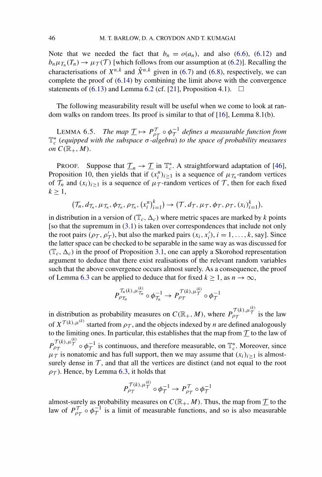
46 M. T. BARLOW, D. A. CROYDON AND T. KUMAGAI
Note that we needed the fact that bn = o(an), and also (6.6), (6.12) andbnμTn(Tn) → μT (T ) [which follows from our assumption at (6.2)]. Recalling thecharacterisations of Xn,k and Xn,k given in (6.7) and (6.8), respectively, we cancomplete the proof of (6.14) by combining the limit above with the convergencestatements of (6.13) and Lemma 6.2 (cf. [21], Proposition 4.1). �
The following measurability result will be useful when we come to look at ran-dom walks on random trees. Its proof is similar to that of [16], Lemma 8.1(b).
LEMMA 6.5. The map T �→ P TρT ◦ φ−1
T defines a measurable function fromT∗
c (equipped with the subspace σ -algebra) to the space of probability measureson C(R+,M).
PROOF. Suppose that T n → T in T∗c . A straightforward adaptation of [46],
Proposition 10, then yields that if (xni )i≥1 is a sequence of μTn-random vertices
of Tn and (xi)i≥1 is a sequence of μT -random vertices of T , then for each fixedk ≥ 1, (
Tn, dTn,μTn, φTn, ρTn,(xni
)ki=1
) → (T , dT ,μT , φT , ρT , (xi)
ki=1
),
in distribution in a version of (Tc,�c) where metric spaces are marked by k points[so that the supremum in (3.1) is taken over correspondences that include not onlythe root pairs (ρT , ρ′
T ), but also the marked pairs (xi, x′i), i = 1, . . . , k, say]. Since
the latter space can be checked to be separable in the same way as was discussed for(Tc,�c) in the proof of Proposition 3.1, one can apply a Skorohod representationargument to deduce that there exist realisations of the relevant random variablessuch that the above convergence occurs almost surely. As a consequence, the proofof Lemma 6.3 can be applied to deduce that for fixed k ≥ 1, as n → ∞,
PTn(k),μ
(k)Tn
ρTn◦ φ−1
Tn→ P
T (k),μ(k)T
ρT ◦ φ−1T
in distribution as probability measures on C(R+,M), where PT (k),μ
(k)T
ρT is the law
of XT (k),μ(k)started from ρT , and the objects indexed by n are defined analogously
to the limiting ones. In particular, this establishes that the map from T to the law of
PT (k),μ
(k)T
ρT ◦ φ−1T is continuous, and therefore measurable, on T∗
c . Moreover, sinceμT is nonatomic and has full support, then we may assume that (xi)i≥1 is almost-surely dense in T , and that all the vertices are distinct (and not equal to the rootρT ). Hence, by Lemma 6.3, it holds that
PT (k),μ
(k)T
ρT ◦ φ−1T → P T
ρT ◦ φ−1T
almost-surely as probability measures on C(R+,M). Thus, the map from T to thelaw of P T
ρT ◦ φ−1T is a limit of measurable functions, and so is also measurable

RANDOM WALK ON THE UNIFORM SPANNING TREE 47
on T∗c . Since P T
ρT ◦ φ−1T is a function of only T [and not the particular sequence
(xi)i≥1], the result follows from a standard argument. �
Suppose that T is a random element of Tc, built on a probability space withprobability measure P, and P-a.s. takes values in T∗
c . The previous lemma tellsus that the annealed law of the process φT (XT ), where the Brownian motion XT
is started from the root, that is,∫Tc
P TρT ◦ φ−1
T (·)dP [cf. (1.6)], is a well-definedprobability measure on C(R+,M). By a Skorohod representation argument, wealso obtain the following as an immediate corollary of Theorem 6.1.
COROLLARY 6.6. Let (Tn, dTn,μTn,φTn, ρTn), n ≥ 1 be a random sequence,and (an)n≥1, (bn)n≥1, (cn)n≥1 be null sequences with bn = o(an), such that (6.2)holds in distribution, and the limit T almost-surely takes values in T∗
c . Then theannealed laws of the processes
(cnφTn
(X
Tn
t/anbn
))t≥0
[cf. (1.5)] converge to the annealed law of φT (XT ), where we assume that XTn
0 =ρTn for each n, and also XT
0 = ρT .
As with Lemmas 3.7 and 3.9, Theorem 6.1 and Corollary 6.6 can be extended tothe noncompact case with an additional assumption. To begin with the determin-istic case, suppose (Tn)n≥1 is a deterministic sequence of locally finite graph treesfor which (6.2) holds in (T,�), where T is such that μT is nonatomic, supportedon the leaves of T , and satisfies (6.1) when the infimum is taken over BT (ρT ,R)
for any R; we denote the subset of T whose elements satisfy these properties by T∗.(Note that for an element of T∗, it is possible to define Brownian motion XT on(T , dT ,μT ) by the procedure of [6], as described above the statement of Theo-rem 6.1.) Moreover, assume that, for t > 0,
limR→∞ lim sup
n→∞P Tn
ρTn
(τ(XTn,BTn
(ρTn, a
−1n R
)) ≤ t/anbn
) = 0,
where, here and in the following, τ(X,A) := inf{t ≥ 0 : Xt /∈ A} is the exit timeof a process X from a set A. It is then the case that (6.3) holds. Similarly to Re-marks 3.8 and 3.10, we do not include the full details of this argument, but insteadrestrict our presentation to describing the probabilistic version of the argumentneeded to handle the simple random walk on U . In particular, given Theorems 1.1and 1.3, the key additional ingredient for this is the following, where we recall Pis the annealed law of the simple random walk on U , as introduced at (1.5).
PROPOSITION 6.7. For t > 0,
limR→∞ lim sup
δ→0P
(τ(XU ,BU
(0, δ−κR
)) ≤ tδ−κdw) = 0.

48 M. T. BARLOW, D. A. CROYDON AND T. KUMAGAI
PROOF. Given the volume growth and resistance estimates of [11], Proposi-tion 4.2, we can apply an identical argument to that used to prove the correspondinglimit in [17], Theorem 1.1. �
We are now ready to prove the main simple random walk convergence result forthe UST. In the proof, we let (Pδn)n≥1 be a convergent sequence with limit P, andsuppose that T is a random variable with law P. Unless otherwise noted, we take(M,dM) to be R2 equipped with the Euclidean distance.
PROOF OF THEOREM 1.4(a), (b). As in the proof of Lemma 5.2, the sepa-rability of (T,�) allows us to find realisations of U δn
, n ≥ 1, and T built on acommon probability space with probability measure P∗ such that U δn
→ T holdsin (T,�), P∗-a.s. This yields the existence of a subsequence (ni)i≥1 and diver-gent sequence (rj )j≥1 such that, for every rj , P∗-a.s., we have convergence in
(Tc,�c) of the radius rj restrictions along the subsequence (ni)i≥1, that is, U (rj )
δni
converges to T (rj ). Moreover, since the Lebesgue measure of those r ≥ 0 for whichμT (∂T (r)) > 0 is zero, P-a.s., we may further assume that μT (∂T (rj )) = 0 for ev-ery rj , P-a.s. Noting that the map T �→ T (r) is continuous at those elements of Tsatisfying μT (∂T (r)) = 0 [cf. the proof of Proposition 3.4, and equation (3.5) inparticular], this final condition ensures that, for every rj , T (rj ) is T -measurable.Now, from Theorem 1.3(b)(ii), it is the case that T (r) takes values in T∗
c , P-a.s.[Observe that if r ′ ≤ r/2 and x ∈ T (r), then there exists an x′ ∈ T (r) such thatBT (r) (x, r ′) ⊇ BT (x′, r ′/2), and so there is no problem in deducing the lower vol-ume estimate of (6.1) for the ball T (r) from the lower volume estimate from T .The further two properties—that μ
(r)T is nonatomic and supported on the leaves of
T (r)—are immediate from the full T statements.] Hence, by Corollary 6.6 (withani
= δκni
, bni= δ2
ni, cni
= δni), it follows that, for every rj , the annealed law of
(δni
XBU (0,δ−κ
nirj )
δ−κdwni
t
)t≥0,
where XBU (0,δ−κ
nirj ) is the simple random walk on BU (0, δ−κ
nirj ), converges as i →
∞ to the annealed law of (φ(rj )
T (XT (rj )
t ))t≥0, where XT (rj )
is Brownian motion on
the measured real tree (T (rj ), d(rj )
T ,μ(rj )
T ), and we assume processes are startedfrom the roots of the relevant trees. Given the measurability of T (rj ) describedabove, this limit law can be expressed as∫
P T (rj )
ρT ◦ φ−1T (·) dP.(6.15)
Furthermore, since the limit does not depend on the subsequence, we obtain an-nealed distributional convergence of the rescaled discrete processes along the fullsequence (δn)n≥1.

RANDOM WALK ON THE UNIFORM SPANNING TREE 49
Next, suppose XU and XBU (0,δ−κ
nirj ) are coupled so that their sample paths agree
up to τ(XU ,BU (0, δ−κni
rj )) [e.g., by taking XBU (0,δ−κ
nirj ) to be XU observed on
BU (0, δ−κni
rj )]. It then holds that, for t < ∞ and ε > 0,
P(
sups∈[0,t]
δn
∣∣XUδ−κdwn s
− XBU (0,δ−κ
n rj )
δ−κdwn s
∣∣ > ε)
≤ P(τ(XU ,BU
(0, δ−κ
n rj)) ≤ tδ−κdw
).
Hence, we deduce from Proposition 6.7 that the left-hand side converges to 0 asn → ∞ and then j → ∞.
Finally, we need to take care of the situation when rj → ∞ for the continuous
trees. We have already established that P T (rj )
ρT ◦ φ−1T is T -measurable for every
rj . To show that this is also the case for P TρT ◦ φ−1
T , it will suffice to check that
P T (r)
ρT → P TρT as r → ∞, P-a.s. This will follow if we can check that
P TρT
(lim
r→∞ τ(XT ,BT (ρT , r)
) = ∞)
= 1,(6.16)
for P-a.e. realisation of T . To this end, first note that
P TρT
(lim
r→∞ τ(XT ,BT (ρT , r)
)< ∞
)(6.17)
= limt→∞ lim
r→∞ limj→∞P T (rj )
ρT
(τ(XT (rj )
,BT (ρT , r)) ≤ t
),
where we note that the laws of XT and XT (rj )
agree up to the exit time ofBT (ρT , r) whenever rj > r . Now, suppose that U δn
, n ≥ 1, and T are cou-pled as in the first part of the proof. It is not difficult to check from the defi-nition of �c that the convergence in (Tc,�c) of the radius rj restrictions stillholds P∗-a.s. if δnφU is replaced by δκ
n φU and φT is replaced by φT , whereφU (x) := (dU (0, x),0) and φT (x) := (dT (0, x),0), respectively. Thus, an appli-cation of Theorem 6.1 (with M = R) and a subsequence argument yields that, for
every rj , P∗-a.s., (δκndU (0,X
BU (0,δ−κn rj )
δ−κdwn t
))t≥0 converges to (dT (ρT ,XT (rj )
t ))t≥0 in
distribution in C(R+,R) as n → ∞. Consequently,∫
P T (rj )
ρT
(τ(XT (rj )
,BT (ρT , r)) ≤ t
)dP
=∫
P T (rj )
ρT
(sup
s∈[0,t]dT
(ρT ,XT (rj )
s
) ≥ r)dP
≤∫
lim infn→∞ P
BU (0,δ−κni
rj )
0
(sup
s∈[0,t]dU
(0,X
BU (0,δ−κn rj )
δ−κdwn s
) ≥ δ−κn r/2
)dP
≤ lim infn→∞ P
(τ(XBU (0,δ−κ
n rj ),BU(0, δ−κ
n r)) ≤ tδ−κdw
n
),

50 M. T. BARLOW, D. A. CROYDON AND T. KUMAGAI
where we note that the necessary measurability of the law of dT (ρT ,XT (rj )
) can
be checked similarly to the measurability of P T (rj )
ρT ◦φ−1T . Taking limits as j → ∞,
r → ∞ and then t → ∞, we obtain from another application of Proposition 6.7that the upper bound above converges to zero. Thus, the dominated convergencetheorem yields that the P-expectation of the left-hand side of (6.17) is equal tozero, and so we have established (6.16), as desired. In summary, we have nowshown that P T
ρT ◦ φ−1T is T -measurable, and so P—the annealed law of φT (XT ),
as introduced at (1.6)—is well-defined. This establishes part (a) of the theorem.Moreover, since P T (r)
ρT → P TρT , P-a.s., the continuous mapping theorem and the
dominated convergence theorem yield that the annealed law at (6.15) converges asj → ∞ to P. Together with the conclusions of the previous two paragraphs, thiscompletes the proof of part (b) (see [13], Theorem 3.2, e.g.). �
REMARK 6.8. In [20], Theorem 8.1, it was shown that the convergence ofrescaled graph tree “tours” (i.e., functions encoding trees and embeddings into Rd )implies convergence of spatial trees. It only requires a simple extension of theproof of that result to add the measure, and thereby deduce that convergence oftours also implies convergence in the topology of (Tc,�c) (with R2 replacedby Rd ). Consequently, (the Rd version of) Theorem 6.1 provides an extension ofthe random walk convergence result of [20], Theorem 8.1, and can also be used todeduce a scaling limit for the simple random walks on critical branching randomwalks satisfying the various assumptions on the offspring and step distribution de-tailed in [20], Section 10.
REMARK 6.9. In [21], Theorem 1.1 (see also [16], Theorem 1.1), a scalinglimit was established for simple random walks on ordered graph trees. The proofsof these results used the convenience of encoding ordered graph trees by func-tions to simplify various technical details. Theorem 6.1 provides the additionalframework needed to handle unordered graph trees. Indeed, suppose that we havea sequence of finite rooted graph trees such that
(Tn, andTn, bnμTn, ρTn) → (T , dT ,μT , ρT ),(6.18)
for some null sequences (an)n≥1 and (bn)n≥1 with bn = o(an) in the Gromov–Hausdorff–Prohorov topology of [1] for rooted, compact metric spaces equippedwith Borel measures. Moreover, assume that the limit satisfies the additional prop-erties on the measure that hold for elements of T∗
c . It is then the case that, by ap-plying the procedure described in the proof of Lemma 6.3, one can find isometricembeddings ψ : T → �1 and ψn : Tn → �1, n ≥ 1, such that
(anψn
(X
Tn
t/anbn
))t≥0 → (
ψ(XT
t
))t≥0,
in distribution in C(R+, �1), where XTn is the simple random walk on Tn startedfrom ρTn , and XT is the Brownian motion on (T , dT ,μT ) started from ρT . We

RANDOM WALK ON THE UNIFORM SPANNING TREE 51
note that a similar, but slightly stronger result was recently established indepen-dently in [7]—the most important difference being that the argument of the latterwork required a weaker lower volume growth condition.
The above result can also be extended to the random case by embeddingtrees into �1 in a canonical random way—specifically, by choosing the vertices(xi)i≥1 ∈ T to be a μT -random sequence. The only additional complicationscome from some measurability issues, but these can be resolved using similarideas to those applied in the proof of Lemma 6.5. To summarise the conclusion,suppose that (Tn)n≥1 is a sequence of finite rooted (unordered) graph trees forwhich (6.18) holds in distribution for some random measured compact real tree(T , dT ,μT , ρT ). Moreover, assume that μT is a nonatomic probability measure,supported on the leaves of T and satisfies (6.1), almost-surely. It can then bechecked that the annealed laws of (anψn(X
Tn
t/anbn))t≥0, where ψn is the canoni-
cal random isometric embedding of Tn into �1, converge to the annealed law ofBrownian motion on T randomly isometrically embedded into �1. For example,taking an = n−1/2, bn = n−1, this result applies to the model of uniformly randomunordered trees with n vertices, in which each vertex has at most m ∈ {2,3, . . . ,∞}children, as studied in [28]. Moreover, applying the argument of [22], Section 5.2,(where critical Galton–Watson trees were considered), a corollary of this is thatthe mixing times of the simple random walks on the random discrete trees, whenrescaled by n3/2, converge in distribution to (a constant multiple of) the mixingtime of the limiting diffusion.
7. Heat kernel bounds for the scaling limit. As in Section 5 and the proof ofTheorem 1.4(a), (b), let (Pδn)n≥1 be a convergent sequence with limit P, and sup-pose that (T , dT ,μT , φT , ρT ) is a random variable with law P. It follows from [6],Remark 3.1 and [27], Theorem 1.5.2, that the Dirichlet form (ET ,FT ) given inSection 6 is the same as that of [32], Section 5. In particular, this is the form as-sociated with the natural “resistance form” on (T , dT ), and so we can apply [33],Theorem 10.4, to deduce the existence of a jointly continuous transition density(pT
t (x, y))x,y∈T ,t>0 for the process XT .Let RT be the resistance associated with (ET ,FT ), defined by setting, for two
disjoint subsets A,B ⊆ T ,
RT (A,B)−1 := inf{ET (f, f ) : f ∈ FT , f |A = 0, f |B = 1
}.
Since T is complete and, by Theorem 1.3(a)(ii), has a single end at infinity, wededuce from [6], Theorem 4, that XT is recurrent. As a consequence, combin-ing [27], Theorem 1.6.3 and [6], Proposition 3.5, yields that the resistance be-tween two points corresponds to (a multiple of) the distance between them, thatis, RT ({x}, {y}) = 2dT (x, y) for all x, y ∈ T , x �= y (see [6], e.g.). Hence, we canuse [18], Theorem 3, to obtain estimates for pT
t (x, y) from the volume estimatesof Theorem 1.3(b)(ii).

52 M. T. BARLOW, D. A. CROYDON AND T. KUMAGAI
PROOF OF THEOREM 1.4(c). We have already discussed the claims about theexistence and joint continuity of the heat kernel, and the recurrence of XT . So, wewill simply present here a few key points that are needed to apply the heat kernelestimates of [18], Theorem 3. As already noted, the resistance metric coincideswith (a multiple of) the tree metric dT in our setting, and so we can replace RT inthe conclusion of [18] by dT . Moreover, the fact that (T , dT ) is a real tree automat-ically means the “chaining condition” of [18] is satisfied, that is, there exists a con-stant c1 such that for all x, y ∈ T and all n ∈ N, there exist x0 = x, x1, . . . , xN = y
such that dT (xi−1, xi) ≤ c1dT (x, y)/n, ∀i = 1, . . . , n. (Clearly, we can take c1 = 1and equality in the latter statement.) Finally, note that in [18] volume estimateswere assumed to hold uniformly over the entire space, but Theorem 1.3(b)(ii) onlygives uniformity over balls of finite radius. However, it is straightforward to checkthat the arguments of [18] are enough to give the stated heat kernel estimates. �
For the remaining heat kernel estimates, we derive the following tail bound forthe resistance from the root to the radius of a ball will be useful.
LEMMA 7.1. There exist constants c1, c2, θ ∈ (0,∞) such that for all r > 0,λ ≥ 1,
P(RT
(ρT ,BT (ρT , r)c
) ≤ λ−1r) ≤ c1e
−c2λθ
.(7.1)
PROOF. As we have done several times previously, we will apply a cou-pling argument, and start by supposing that we have a realisation of randomvariables such that U δn
→ T holds almost-surely along the sequence (δn)n≥1.Let NT (r, r/λ) be the minimum number of dT -balls of radius r/λ required tocover BT (ρT , r). From the definition of (T,�), it is elementary to check that ifNT (r, r/λ) ≥ N0, then so is NU (4δ−κ
n r, δ−κn r/8λ) for large n. It follows that
P(NT (r, r/λ) ≥ cλ5) ≤ lim sup
n→∞P
(NU
(4δ−κ
n r, δ−κn r/8λ
) ≥ cλ5),(7.2)
which by Remark 2.13 is, for a suitable choice of c, bounded above by c1e−c2λ
1/80.
Now, the proof of [35], Lemma 4.1, gives that RT (ρT ,BT (ρT , r)c) ≥ r/8NT (r,
r/4), and so, for any λ > 45c,
P(RT
(ρT ,BT (ρT , r)c
) ≤ r/λ) ≤ P
(NT
(r, c1/5r/λ1/5) ≥ 8λ
).
Combining this bound with (7.2) yields the result. �
Given (5.16), (5.17) and (7.1), the next two results can be proved in exactlythe same way as the corresponding parts of [19], Theorem 1.6 and [19], Proposi-tion 1.7, modulo a different volume growth exponent.

RANDOM WALK ON THE UNIFORM SPANNING TREE 53
THEOREM 7.2. (a) P-a.s., there exists a random t0(T ) ∈ (0,∞) and deter-ministic constants c1, c2, θ1, θ2 ∈ (0,∞) such that
c1t−8/13(
log log t−1)−θ1 ≤ pTt (ρT , ρT ) ≤ c2t
−8/13(log log t−1)θ2,
for all t ∈ (0, t0).(b) There exist constants c1, c2 ∈ (0,∞) such that
c1t−8/13 ≤ EpT
t (ρT , ρT ) ≤ c2t−8/13,
for all t ∈ (0,1).
Acknowledgement. The authors thank Sunil Chhita, who wrote the code usedto produce Figure 1.
REFERENCES
[1] ABRAHAM, R., DELMAS, J.-F. and HOSCHEIT, P. (2013). A note on the Gromov–Hausdorff–Prokhorov distance between (locally) compact metric measure spaces. Electron. J.Probab. 18 1–21. MR3035742
[2] AIZENMAN, M., BURCHARD, A., NEWMAN, C. M. and WILSON, D. B. (1999). Scalinglimits for minimal and random spanning trees in two dimensions. Random StructuresAlgorithms 15 319–367. MR1716768
[3] ALBERTS, T., KOZDRON, M. J. and MASSON, R. (2013). Some partial results on the conver-gence of loop-erased random walk to SLE(2) in the natural parametrization. J. Stat. Phys.153 119–141. MR3100817
[4] ALDOUS, D. (1993). The continuum random tree. III. Ann. Probab. 21 248–289. MR1207226[5] ALDOUS, D. J. (1990). The random walk construction of uniform spanning trees and uniform
labelled trees. SIAM J. Discrete Math. 3 450–465. MR1069105[6] ATHREYA, S., ECKHOFF, M. and WINTER, A. (2013). Brownian motion on R-trees. Trans.
Amer. Math. Soc. 365 3115–3150. MR3034461[7] ATHREYA, S., LÖHR, W. and WINTER, A. (2014). Invariance principle for variable speed
random walks on trees. Preprint. Available at arXiv:1404.6290.[8] BARLOW, M. T. (2016). Loop erased walks and uniform spanning trees. MSJ Memoirs 34
1–32. MR3525847[9] BARLOW, M. T., JÁRAI, A. A., KUMAGAI, T. and SLADE, G. (2008). Random walk on the
incipient infinite cluster for oriented percolation in high dimensions. Comm. Math. Phys.278 385–431. MR2372764
[10] BARLOW, M. T. and MASSON, R. (2010). Exponential tail bounds for loop-erased randomwalk in two dimensions. Ann. Probab. 38 2379–2417. MR2683633
[11] BARLOW, M. T. and MASSON, R. (2011). Spectral dimension and random walks on the twodimensional uniform spanning tree. Comm. Math. Phys. 305 23–57. MR2802298
[12] BENJAMINI, I., LYONS, R., PERES, Y. and SCHRAMM, O. (2001). Uniform spanning forests.Ann. Probab. 29 1–65. MR1825141
[13] BILLINGSLEY, P. (1999). Convergence of Probability Measures, 2nd ed. Wiley, New York.MR1700749
[14] BRODER, A. (1989). Generating random spanning trees. In Proceedings of the 30th AnnualSymposium on Foundations of Computer Science 442–447. IEEE Computer Society,Washington, DC.

54 M. T. BARLOW, D. A. CROYDON AND T. KUMAGAI
[15] BURAGO, D., BURAGO, Y. and IVANOV, S. (2001). A Course in Metric Geometry. GraduateStudies in Mathematics 33. Amer. Math. Soc., Providence, RI. MR1835418
[16] CROYDON, D. (2008). Convergence of simple random walks on random discrete trees to Brow-nian motion on the continuum random tree. Ann. Inst. Henri Poincaré Probab. Stat. 44987–1019. MR2469332
[17] CROYDON, D. and KUMAGAI, T. (2008). Random walks on Galton–Watson trees with infinitevariance offspring distribution conditioned to survive. Electron. J. Probab. 13 1419–1441.MR2438812
[18] CROYDON, D. A. (2007). Heat kernel fluctuations for a resistance form with non-uniformvolume growth. Proc. Lond. Math. Soc. (3) 94 672–694. MR2325316
[19] CROYDON, D. A. (2008). Volume growth and heat kernel estimates for the continuum randomtree. Probab. Theory Related Fields 140 207–238. MR2357676
[20] CROYDON, D. A. (2009). Hausdorff measure of arcs and Brownian motion on Brownian spatialtrees. Ann. Probab. 37 946–978. MR2537546
[21] CROYDON, D. A. (2010). Scaling limits for simple random walks on random ordered graphtrees. Adv. in Appl. Probab. 42 528–558. MR2675115
[22] CROYDON, D. A., HAMBLY, B. M. and KUMAGAI, T. (2012). Convergence of mixingtimes for sequences of random walks on finite graphs. Electron. J. Probab. 17 1–32.MR2869250
[23] DUQUESNE, T. and LE GALL, J.-F. (2005). Probabilistic and fractal aspects of Lévy trees.Probab. Theory Related Fields 131 553–603. MR2147221
[24] EDGAR, G. A. (1998). Integral, Probability, and Fractal Measures. Springer, New York.MR1484412
[25] EVANS, S. N. (2008). Probability and Real Trees. Lecture Notes in Math. 1920. Springer,Berlin. MR2351587
[26] EVANS, S. N., PITMAN, J. and WINTER, A. (2006). Rayleigh processes, real trees, and rootgrowth with re-grafting. Probab. Theory Related Fields 134 81–126. MR2221786
[27] FUKUSHIMA, M., OSHIMA, Y. and TAKEDA, M. (1994). Dirichlet Forms and Symmet-ric Markov Processes. De Gruyter Studies in Mathematics 19. de Gruyter, Berlin.MR1303354
[28] HAAS, B. and MIERMONT, G. (2012). Scaling limits of Markov branching trees with ap-plications to Galton–Watson and random unordered trees. Ann. Probab. 40 2589–2666.MR3050512
[29] HÄGGSTRÖM, O. (1995). Random-cluster measures and uniform spanning trees. StochasticProcess. Appl. 59 267–275. MR1357655
[30] KALLENBERG, O. (2002). Foundations of Modern Probability, 2nd ed. Springer, New York.MR1876169
[31] KENYON, R. (2000). The asymptotic determinant of the discrete Laplacian. Acta Math. 185239–286. MR1819995
[32] KIGAMI, J. (1995). Harmonic calculus on limits of networks and its application to dendrites.J. Funct. Anal. 128 48–86. MR1317710
[33] KIGAMI, J. (2012). Resistance forms, quasisymmetric maps and heat kernel estimates. Mem.Amer. Math. Soc. 216 vi+132. MR2919892
[34] KIRCHHOFF, G. (1847). Ueber die Auflösung der Gleichungen, auf welche man bei der Un-tersuchung der linearen Vertheilung galvanischer Ströme geführt wird. Ann. Phys. 148497–508.
[35] KUMAGAI, T. (2004). Heat kernel estimates and parabolic Harnack inequalities on graphs andresistance forms. Publ. Res. Inst. Math. Sci. 40 793–818. MR2074701
[36] KUMAGAI, T. (2014). Random Walks on Disordered Media and Their Scaling Limits. LectureNotes in Math. 2101. Springer, Cham. MR3156983

RANDOM WALK ON THE UNIFORM SPANNING TREE 55
[37] KUMAGAI, T. and MISUMI, J. (2008). Heat kernel estimates for strongly recurrent randomwalk on random media. J. Theoret. Probab. 21 910–935. MR2443641
[38] LAWLER, G. F. (1999). Loop-erased random walk. In Perplexing Problems in Probability(M. Bramson and R. Durrett, eds.). Progress in Probability 44 197–217. Birkhäuser,Boston, MA. MR1703133
[39] LAWLER, G. F. (2013). Intersections of Random Walks. Birkhäuser/Springer, New York.MR2985195
[40] LAWLER, G. F. (2014). The probability that planar loop-erased random walk uses a given edge.Electron. Commun. Probab. 19 1–13. MR3246970
[41] LAWLER, G. F., SCHRAMM, O. and WERNER, W. (2004). Conformal invariance of pla-nar loop-erased random walks and uniform spanning trees. Ann. Probab. 32 939–995.MR2044671
[42] LAWLER, G. F. and SHEFFIELD, S. (2011). A natural parametrization for the Schramm–Loewner evolution. Ann. Probab. 39 1896–1937. MR2884877
[43] LAWLER, G. F. and ZHOU, W. (2013). SLE curves and natural parametrization. Ann. Probab.41 1556–1584. MR3098684
[44] LE GALL, J.-F. (2006). Random real trees. Ann. Fac. Sci. Toulouse Math. (6) 15 35–62.MR2225746
[45] MASSON, R. (2009). The growth exponent for planar loop-erased random walk. Electron. J.Probab. 14 1012–1073. MR2506124
[46] MIERMONT, G. (2009). Tessellations of random maps of arbitrary genus. Ann. Sci. Éc. Norm.Supér. (4) 42 725–781. MR2571957
[47] PEMANTLE, R. (1991). Choosing a spanning tree for the integer lattice uniformly. Ann. Probab.19 1559–1574. MR1127715
[48] SCHRAMM, O. (2000). Scaling limits of loop-erased random walks and uniform spanning trees.Israel J. Math. 118 221–288. MR1776084
[49] WILSON, D. B. (1996). Generating random spanning trees more quickly than the cover time. InProceedings of the Twenty-Eighth Annual ACM Symposium on the Theory of Computing(Philadelphia, PA, 1996) 296–303. ACM, New York. MR1427525
M. T. BARLOW
DEPARTMENT OF MATHEMATICS
UNIVERSITY OF BRITISH COLUMBIA
VANCOUVER, B.C., V6T 1Z2CANADA
E-MAIL: [email protected]
D. A. CROYDON
DEPARTMENT OF STATISTICS
UNIVERSITY OF WARWICK
COVENTRY, CV4 7ALUNITED KINGDOM
E-MAIL: [email protected]
T. KUMAGAI
RESEARCH INSTITUTE FOR MATHEMATICAL SCIENCES
KYOTO UNIVERSITY
KYOTO 606-8502JAPAN
E-MAIL: [email protected]