SUBJECT : Math TITLE OF COURSE : Algebra 1 GRADE … school 1… · Unit 1: Quantities and Modeling Module 2: Algebraic Models 2.4: Creating and solving inequalities Creating and

Ref: GIS Math G 8 A.E. 2015-2016

2011-2012

SUBJECT : Math TITLE OF COURSE : Algebra 1

GRADE LEVEL : 8

DURATION : ONE YEAR

NUMBER OF CREDITS : 1.25

Goals:

The Number System 8.NS Know that there are numbers that are not rational, and approximate them by rational numbers. 1. Know that numbers that are not rational are called irrational. Understand informally that every number has a decimal expansion; for rational numbers show that the decimal expansion repeats eventually, and convert a decimal expansion which repeats eventually into a rational number. 2. Use rational approximations of irrational numbers to compare the size of irrational numbers, locate them approximately on a number line diagram, and estimate the value of expressions (e.g., π2). For example, by truncating the decimal expansion of √2, show that √2 is between 1 and 2, then between 1.4 and 1.5, and explain how to continue on to get better approximations.

Expressions and Equations 8.EE Work with radicals and integer exponents. 1. Know and apply the properties of integer exponents to generate equivalent numerical

expressions. For example, 32 × 3–5 = 3–3 = 1/33 = 1/27.

2. Use square root and cube root symbols to represent solutions to equations of the form x2 = p and x3 = p, where p is a positive rational number. Evaluate square roots of small perfect squares and cube roots of small perfect cubes. Know that √2 is irrational. 3. Use numbers expressed in the form of a single digit times an integer power of 10 to estimate very large or very small quantities, and to express how many times as much

one is than the other. For example, estimate the population of the United States as 3×

108 and the population of the world as 7 × 109, and determine that the world

population is more than 20 times larger. 4. Perform operations with numbers expressed in scientific notation, including problems where both decimal and scientific notation are used. Use scientific notation and choose

units of appropriate size for measurements of very large or very small quantities (e.g., use millimeters per year for seafloor spreading). Interpret scientific notation that has been generated by technology.

Understand the connections between proportional relationships, lines, and linear equations. 5. Graph proportional relationships, interpreting the unit rate as the slope of the graph. Compare two different proportional relationships represented in different ways. For example, compare a distance-time graph to a distance-time equation to determine which of two moving objects has greater speed. 6. Use similar triangles to explain why the slope m is the same between any two distinct points on a non-vertical line in the coordinate plane; derive the equation y = mx for a line through the origin and the equation y = mx + b for a line intercepting the vertical axis at b.

Analyze and solve linear equations and pairs of simultaneous linear equations. 7. Solve linear equations in one variable. a. Give examples of linear equations in one variable with one solution, infinitely many solutions, or no solutions. Show which of these possibilities is the case by successively transforming the given equation into simpler forms, until an equivalent equation of the form x = a, a = a, or a = b results (where a and b are different numbers). b. Solve linear equations with rational number coefficients, including equations whose solutions require expanding expressions using the distributive property and collecting like terms. 8. Analyze and solve pairs of simultaneous linear equations. a. Understand that solutions to a system of two linear equations in two variables correspond to points of intersection of their graphs, because points of intersection satisfy both equations simultaneously. b. Solve systems of two linear equations in two variables algebraically, and estimate solutions by graphing the equations. Solve simple cases by inspection. For example, 3x + 2y = 5 and 3x + 2y = 6 have no solution because 3x + 2y cannot simultaneously be 5 and 6. c. Solve real-world and mathematical problems leading to two linear equations in two variables. For example, given coordinates for two pairs of points, determine whether the line through the first pair of points intersects the line through the second pair.

Functions 8.F Define, evaluate, and compare functions. 1. Understand that a function is a rule that assigns to each input exactly one output. The graph of a function is the set of ordered pairs consisting of an input and the corresponding output.1 2. Compare properties of two functions each represented in a different way (algebraically, graphically, numerically in tables, or by verbal descriptions). For example, given a linear function represented by a table of values and a linear function represented by an algebraic expression, determine which function has the greater rate of change. 3. Interpret the equation y = mx + b as defining a linear function, whose graph is a straight line; give examples of functions that are not linear.

For example, the function A = s2 giving the area of a square as a function of its side length is not linear because its graph contains the points (1,1),(2, 4) and (3, 9), which are not on a straight line.

Use functions to model relationships between quantities. 4. Construct a function to model a linear relationship between two quantities. Determine the rate of change and initial value of the function from a description of a relationship or from two (x, y) values, including reading these from a table or from a graph. Interpret the rate of change and initial value of a linear function in terms of the situation it models, and in terms of its graph or a table of values. 5. Describe qualitatively the functional relationship between two quantities by analyzing a graph (e.g., where the function is increasing or decreasing, linear or nonlinear). Sketch a graph that exhibits the qualitative features of a function that has been described verbally.

Geometry 8.G Understand congruence and similarity using physical models, transparencies, or geometry software. 1. Verify experimentally the properties of rotations, reflections, and translations: a. Lines are taken to lines, and line segments to line segments of the same length. b. Angles are taken to angles of the same measure. c. Parallel lines are taken to parallel lines. 2. Understand that a two-dimensional figure is congruent to another if the second can be obtained from the first by a sequence of rotations, reflections, and translations; given two congruent figures, describe a sequence that exhibits the congruence between them. 3. Describe the effect of dilations, translations, rotations, and reflections on two-dimensional figures using coordinates. 4. Understand that a two-dimensional figure is similar to another if the second can be obtained from the first by a sequence of rotations, reflections, translations, and dilations; given two similar two dimensional figures, describe a sequence that exhibits the similarity between them. 5. Use informal arguments to establish facts about the angle sum and exterior angle of triangles, about the angles created when parallel lines are cut by a transversal, and the angle-angle criterion for similarity of triangles. For example, arrange three copies of the same triangle so that the sum of the three angles appears to form a line, and give an argument in terms of transversals why this is so.

Understand and apply the Pythagorean Theorem. 6. Explain a proof of the Pythagorean Theorem and its converse. 7. Apply the Pythagorean Theorem to determine unknown side lengths in right triangles in real-world and mathematical problems in two and three dimensions. 8. Apply the Pythagorean Theorem to find the distance between two points in a coordinate system.

Solve real-world and mathematical problems involving volume of cylinders, cones, and spheres. 9. Know the formulas for the volumes of cones, cylinders, and spheres and use them to solve real-world and mathematical problems.

Statistics and Probability 8.SP Investigate patterns of association in bivariate data.

1. Construct and interpret scatter plots for bivariate measurement data to investigate patterns of association between two quantities. Describe patterns such as clustering, outliers, positive or negative association, linear association, and nonlinear association. 2. Know that straight lines are widely used to model relationships between two quantitative variables. For scatter plots that suggest a linear association, informally fit a straight line, and informally assess the model fit by judging the closeness of the data points to the line. 3. Use the equation of a linear model to solve problems in the context of bivariate measurement data, interpreting the slope and intercept. For example, in a linear model for a biology experiment, interpret a slope of 1.5 cm/hr as meaning that an additional hour of sunlight each day is associated with an additional 1.5 cm in mature plant height. 4. Understand that patterns of association can also be seen in bivariate categorical data by displaying frequencies and relative frequencies in a two-way table. Construct and interpret a two-way table summarizing data on two categorical variables collected from the same subjects. Use relative frequencies calculated for rows or columns to describe possible association between the two variables. For example, collect data from students in your class on whether or not they have a curfew on school nights and whether or not they have assigned chores at home. Is there evidence that those who have a curfew also tend to have chores?

Resources: 1- HMH Algebra 1 text book.

2- Online resources

3- HMH attached resources CD’S (lesson tutorial videos, power point presentations, one

stop

planer,…..)

4- Internet.

5- E-games and links

6- Teacher’s Handouts

Course Content and Objectives: Unit 1: Quantities and Modeling

Module 2: Algebraic Models

2.2: Creating and solving equations

Creating and solving equations

Solving proportions

2.3: Solving for a variable

Algebraic expressions

Solving for a variable

Creating and solving inequalities

Unit 1: Quantities and Modeling


2.4: Creating and solving inequalities

Creating and solving equations

Solving proportions

2.5: Creating and solving compound inequalities

Algebraic expressions

Solving for a variable

Creating and solving inequalities

Unit 3: Linear functions, equations, and inequalities

Module 7: Linear equations and inequalities

7.1: Modeling linear relationships

Linear functions

Rate of change and slope

7.2: Using functions to solve one-variable equations

Slope intercept form and point-slope form

Modeling linear relationships

Using functions to solve one-variable equations

Linear inequalities in two variables

7.3: Linear inequalities in two variables

Linear functions






Unit 2: Understanding functions

Module 3: Functions and models

3.1: Graphing relationships

Graphing relationships

Understanding relations and functions

Modeling functions

Graphing functions

3.2: Understanding relations and functions

Identifying and graphing sequences

Constructing and modeling arithmetic sequences

3.3: Modeling with functions

Graphing relationships

Understanding relations and functions

Modeling functions

3.4: Graphing functions

Graphing functions

Identifying and graphing sequences

Constructing and modeling arithmetic sequences

Unit 3: Linear functions, equations, and inequalities

Module 5: Linear functions

5.1: Understanding linear functions

Linear functions



5.2: Using intercepts




5.3: Interpreting rate of change and slope

Linear functions






Module 6: Forms of linear equations

6.1: Slope- intercept form

Linear functions






6.2: Point-slope form

Linear functions



6.3: Standard form




Unit 5: Linear systems and piecewise-defined functions

Module 11: Solving systems of linear equations

11.1: Solving linear systems by graphing

Solving systems of linear equations

Creating systems of linear equations

11.2: Solving linear systems by substitution

Graphing systems of linear equalities and inequalities

Solving absolute value equations and inequalities

11.3: Solving linear systems by adding or subtracting Solving systems of linear equations


11.4: Solving linear systems by multiplying first



Module 12: Modeling with linear systems

12.1: Creating systems of linear equations



12.2: Graphing systems of linear inequalities



12.3: Modeling with linear systems





Unit 8: Quadratic functions

Module 19: Graphing quadratic functions

19.1: Understanding quadratic functions

Graphing quadratic functions

Interpreting vertex and standard form of quadratic functions

Connecting intercepts and zeros

Solving quadratic equations using the zero product property

Unit 7: Polynomial Operations

Module 17: Adding and subtracting polynomials

17.1: Understanding polynomial expressions

Adding polynomial expressions

Subtracting polynomial expressions

Multiplying polynomial expressions

17.2: Adding polynomials expressions

Special products of binomials

Dividing polynomial expressions Module 19: Graphing quadratic functions

19.2: Transforming quadratic functions



19.3: Interpreting vertex form and standard form



Unit 8: Quadratic functions

Module 20: Connecting intercepts and zeros

20.1: Connecting intercepts and zeros



20.2: Connecting intercepts and linear factors



20.3: Apply the zero product property to solve equations





Unit 9: Quadratic equations and modeling

Module 21: Using factors to solve quadratic equations

21.1: Solving equations by factoring x2+bx+c

Solving quadratic equations by factoring

Solving quadratic equations by completing the square

Using the quadratic formula to solve equations

Comparing linear, quadratic, and exponential models

21.2: Solving equations by factoring ax2+ bx + c



21.3: Using special factors to solve equations



Module 22: Using square roots to solve quadratic equations

22.1: Solving equations by taking square roots


Solving quadratic equations by completing

22.2: Solving equations by completing the square



22.3: Using the quadratic formula to solve equations



22.4: Choosing a method for solving quadratic equations



22.5: Solving non-linear systems





Unit 6: Exponential relationships

Module 14: Rational exponents and radicals

14.1: Understanding rational exponents and radicals

Simplifying expressions with rational exponents

Simplifying expressions with radicals

14.2: Simplifying expressions with rational exponents and radicals

Geometric sequences

Exponential functions

Module 15: Geometric Sequences and exponential functions

15.1: Understanding geometric sequences



15.2: Constructing geometric sequences

Geometric sequences


15.3: Constructing exponential functions



15.4: Graphing exponential functions

Geometric sequences


15.5: Transforming exponential functions



Geometric sequences


Unit 9: Quadratic equations and modeling


23.1: Modeling with quadratic functions



23.2: Comparing linear, exponential, and quadratic models



Unit 10: Inverse relationships

Module 24: Functions and inverses

24.1: Graphing polynomial functions

Graphing polynomial functions

Understanding inverse functions

Graphing square root functions

24.2: Understanding inverse functions

Graphing cube root functions

24.3: Graphing square root functions

Graphing polynomial functions

Understanding inverse functions

Graphing square root functions

24.4: Graphing cube root functions

Graphing cube root functions

Unit 5: Linear systems and piecewise-defined functions

Module 13: Piecewise-defined functions

13.1: Understanding piecewise-defined functions



13.2: Absolute value functions and transformations



Unit 4: Statistical Models

Module 8: Multi-variable categorical data

8.1: Two-way frequency tables

Multi-variable data and two-way frequency tables

Measures of center and spread

8.2: Relative frequency

Histograms and box plots

Normal distributions

Fitting a linear model to data

Module 9: One-variable data distributions

9.1: Measures of center and spread



9.2: Data distributions and outliers




9.3: Histograms and box plots



9.4: Normal distributions




Course Sequence. Term 1


2.2: Creating and solving equations

2.3: Solving for a variable

2.4: Creating and solving inequalities

2.5: Creating and solving compound inequalities

Module 7: Linear equations and inequalities 7.1: Modeling linear relationships

7.2: Using functions to solve one-variable equations

7.3: Linear inequalities in two variables

Module 3: Functions and models

3.1: Graphing relationships

3.2: Understanding relations and functions

3.3: Modeling with functions

3.4: Graphing functions Module 5: Linear functions

5.1: Understanding linear functions

5.2: Using intercepts

5.3: Interpreting rate of change and slope

Module 6: Forms of linear equations

6.1: Slope intercept form

6.2: Point-slope form

6.3: Standard form

Module 11: Solving systems of linear equations

11.1: Solving linear systems by graphing 11.2: Solving linear systems by substitution

11.3: Solving linear systems by adding or subtracting

11.4: Solving linear systems by multiplying first

Module 12: Modeling with linear systems

12.1: Creating systems of linear equations

12.2: Graphing systems of linear inequalities

12.3: Modeling with linear systems

Module 19: Graphing quadratic functions

19.1: Understanding quadratic functions

Module 17: Adding and subtracting polynomials

17.1: Understanding polynomial expressions

17.2: Adding polynomials expressions

17.3: Subtracting polynomial expressions

Module 18: Multiplying polynomials

18.1: Multiplying polynomial expressions

18.2: Multiplying polynomial expressions

18.3: Special products of binomials

Term 2 Module 19: Graphing quadratic functions 19.2: Transforming quadratic functions 19.3: Interpreting vertex form and standard form

Module 20: Connecting intercepts and zeros 20.3: Apply the zero product property to solve equations

Module 21: Using factors to solve quadratic equations 21.1: Solving equations by factoring x2+bx+c 21.2: Solving equations by factoring a x2+ bx + c

21.3: Using special factors to solve equations

Module 22: Using square roots to solve quadratic equations 22.2: Solving equations by completing the square

22.3: Using the quadratic formula to solve equations

22.4: Choosing a method for solving quadratic equations

22.5: Solving non-linear systems

Module 14: Rational exponents and radicals

14.1: Understanding rational exponents and radicals

14.2: Simplifying expressions with rational exponents and radicals

Module 15: Geometric Sequences and exponential functions

15.1: Understanding geometric sequences

15.2: Constructing geometric sequences

15.3: Constructing exponential functions

15.4: Graphing exponential functions

15.5: Transforming exponential functions

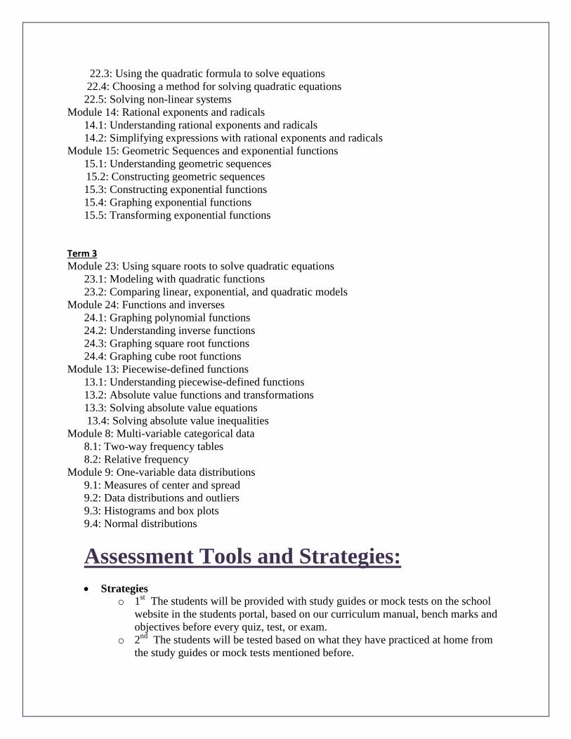
Term 3


23.1: Modeling with quadratic functions

23.2: Comparing linear, exponential, and quadratic models

Module 24: Functions and inverses

24.1: Graphing polynomial functions

24.2: Understanding inverse functions

24.3: Graphing square root functions

24.4: Graphing cube root functions

Module 13: Piecewise-defined functions

13.1: Understanding piecewise-defined functions

13.2: Absolute value functions and transformations

13.3: Solving absolute value equations

13.4: Solving absolute value inequalities

Module 8: Multi-variable categorical data

8.1: Two-way frequency tables

8.2: Relative frequency

Module 9: One-variable data distributions

9.1: Measures of center and spread

9.2: Data distributions and outliers

9.3: Histograms and box plots

9.4: Normal distributions

Assessment Tools and Strategies:

Strategieso 1

st The students will be provided with study guides or mock tests on the school

website in the students portal, based on our curriculum manual, bench marks and

objectives before every quiz, test, or exam.

o 2nd

The students will be tested based on what they have practiced at home from

the study guides or mock tests mentioned before.

o 3rd

The evaluation will be based on what objectives did the students achieve, and

in what objectives do they need help, through the detailed report that will be sent

to the parents once during the semester and once again with the report card.

Tests and quizzes will comprise the majority of the student’s grade. There will be one major test

given at the end of each chapter.

Warm-up problems for review, textbook assignments, worksheets, etc. will comprise the majority of

the daily work.

Home Works and Assignments will provide students the opportunity to practice the concepts

explained in class and in the text.

Students will keep a math notebook. In this notebook students will record responses to daily warm-

up problems, lesson activities, post-lesson wrap-ups, review work, and daily textbook ssignments.

Class work is evaluated through participation, worksheets, class activities and group work done in

the class.

Passing mark 60 %

Grading Policy: Term 1 Terms 2 and 3

Weight Frequency

Weight Frequency

Class Work 15% At least two times

Class Work 20% At least two times

Homework 10% At least 4 times

Homework 15% At least 4 times

Quizzes 30% At least times

Quizzes 35% At least 2 times

Project 10% Once in a term.

Project 15% Once in a term.

Class Participation Includes:

POP Quizzes (3

percent) ,

SPI (3 percent) ,

Problem of the

week (3 percent),

Group work

(3 percent).

Student work (3

percent).

15% Class Participation Includes:

POP Quizzes

(3 percent) ,

SPI (3 percent) ,

Problem of the

week (3

percent),

Group work

(3 percent)

Student work (3

percent).

15%

Mid-Year Exam 20%

Total 100 Total 100

Performance Areas (skills).

Evaluation, graphing, Application, and Analysis of the Mathematical concepts and relating them to daily life, through solving exercises, word problems and applications...

Communication and social skills: through group work, or presentation of their own work.

Technology skills: using digital resources and graphic calculators or computers to solve problems or present their work.

Note: The following student materials are required for this class:

Graph paper.

Scientific Calculator (Casio fx-991 ES Plus)

Done by Eman AL-Saleh. Math teacher

Documents

SUBJECT : Math TITLE OF COURSE : Algebra 1 GRADE … school 1… · Unit 1: Quantities and Modeling Module 2: Algebraic Models 2.4: Creating and solving inequalities Creating and