Sub Module 2.2 Thermoelectric thermometry

Mechanical Measurements Prof. S.P.Venkateshan

Indian Institute of Technology Madras

Sub Module 2.2

Thermoelectric thermometry Thermoelectric thermometry is based on thermoelectric effects or

thermoelectricity discovered in the 19th century. They are:

• Seebeck effect discovered by Thomas Johann Seebeck in 1821

• Peltier effect discovered by Jean Charles Peltier in 1824

• Thomson effect discovered by William Thomson (later Lord

Kelvin) in 1847

The effects referred to above were all observed experimentally by the

respective scientists. All these effects are reversible unlike heat diffusion

(conduction of heat) and Joule heating (due to electrical resistance of the

material) which are irreversible. In discussing the three effects we shall

ignore the above mentioned irreversible processes. It is now recognized that

these three effects are related to each other through the Kelvin relations.

Thermoelectric effects:

Figure 4 Sketch to explain Peltier effect Consider two wires of dissimilar materials connected to form a circuit with two

junctions as shown in Figure 4. Let the two junctions be maintained at

different temperatures as shown by the application of heat at the two

junctions. An electric current will flow in the circuit as indicated with heat

absorption at one of the junctions and heat rejection at the other. This is

referred to as the Peltier effect. The power absorbed or released at the

Current I

T1 T2

A

B



junctions is given by IQP ABP π±== where ABπ is the Peltier voltage (this

expression defines the Peltier emf), PQ is rate at which the heat absorbed or

rejected. The direction of the current will decide whether heat is absorbed or

rejected at the junction. For example, if the electrons move from a region of

lower energy to a region of higher energy as they cross the junction, heat will

be absorbed at the junction. This again depends on the nature of the two

materials that form the junction. The subscript AB draws attention to this fact!

The above relation may be written for the two junctions together as

( )21 TABTAB21AB T,T π−π=π (3)

Figure 5 Sketch to explain Thomson effect Note that the negative sign for the second term on the right hand side is a

consequence of the fact that the electrons move from material A to material B

at junction 1 and from material B to material A at junction 2.

Consider now a single conductor of homogeneous material (wire A alone of

Figure 4) in which a temperature gradient exists. The current I is maintained

by heat absorption or heat rejection along the length of the wire. Note that if

the direction of the current is as shown the electrons move in the opposite

direction. If 12 TT > , the electrons move from a region of higher temperature to

that at a lower temperature. In this case heat will be rejected from the wire.

The expression for heat rejected is ∫σ=1

2

T

TAT dTIQ where TQ is the Thomson

heat and Aσ is the Thomson coefficient for the material. A similar expression

may be written for the Thomson heat in conductor B.

Current I

T1 T2

A

B



Figure 6 Sketch to explain the Seebeck effect If we cut conductor B (or A) as indicated the Seebeck emf appears across the

cut. This emf is due to the combined effects of the Peltier and Thomson

effects. We may write the emf appearing across the cut as

( ) ( )

( ) ( ) ( )∫

∫∫+π−π=

++π−π=+=

2

112

1

2

2

112

T

T BATABTAB

T

T B

T

T ATABTABTPS

dTσ-σ

dTσdTσVVV (4)

We define the Seebeck coefficient ABα through the relation ABs α

dTdV

= . In

differential form, Equation 4 may then be rewritten as (assume dTTT 12 =− )

( )

( ) dTσσddVor

σσdT

dα

dTdV

BAABs

BAAB

ABs

−+π=

−+π

==

(5)

Kelvin relations: Since the thermoelectric effects (Peltier and Thomson effects) are reversible

in nature there is no net entropy change in the arrangement shown in Figure

4.

The entropy changes are due to heat addition or rejection at the junctions due

to Peltier effect and all along the two conductors due to Thomson effect. The

entropy change due to Peltier effect may be obtained as follows:

At junction 1, the entropy change is1

AB

1

1P1P T

IT

Qs

π== . Similarly at junction 2

the entropy change is2

AB

2

BA

2

2P1P T

IT

IT

Qs π−=

π== . Again if we assume that the

A

B

T1 T2

VS



temperature difference is dTTT 12 =− the net change in entropy is

⎟⎠⎞

⎜⎝⎛ π=

TIddsP . The net change in entropy due to Thomson heat in the two

conductors may be written as dTTσσIds BA

T−

= . Combining these two we get

0 dTTσσ

TdT

Td

I

0dTTσσ

TdIdsdsds

BA2AB

AB

BATP

=⎥⎦⎤

⎢⎣⎡ −

+π−π

=

=⎥⎦

⎤⎢⎣

⎡ −+⎟

⎠⎞

⎜⎝⎛ π=+=

(6)

The total entropy change is equated to zero since both the thermoelectric

processes are reversible. The current I can have arbitrary value and hence

the bracketed term must be zero.

From Equation 5 ( ) ABsBA ddVdTσσ π−=− . Introducing this in Equation 6 we get

0T

dT

dVTdT

Td ABs

2ABAB =

π−+π−

π

or SABS

AB TTdTdVT α=α==π (7)

We have renamed the Seebeck coefficient as Sα according to normal practice.

Differentiating Equation 7 we get dTαTdαd ssAB +=π . Introduce this in

Equation 5 to get ( ) dTαdTσσdTαTdαdV SBAsss =−++= or

( ) dTdα

Tσσ sBA −=− (8)

Equations 7 and 8 constitute the Kelvin relations. How do we interpret the Kelvin relations?

The Seebeck, Peltier and Thomson coefficients are normally obtained by

experiments. For this purpose we use the arrangement shown in Figure 6

with the junction labeled 2 maintained at a suitable reference temperature,

normally the ice point (0°C). The junction labeled 1 will then be called the

measuring junction. Data is gathered by maintaining the measuring junction

at different temperatures and noting down the Seebeck voltage. If the

measuring junction is also at the ice point the Seebeck voltage is identically



equal to zero. The data is usually represented by a polynomial of suitable

degree. For example, with Chromel (material A) and Alumel (material B) as

the two wire materials, the expression is a quartic of

form 44

33

221S tatatataV +++= where The Seebeck voltage is in μV and the

temperature is in °C. An inverse relation is also used in practice in the form

4S4

3S3

2S2S1 VAVAVAVAt +++= . Two examples follow. We shall see later that the

coefficients in the polynomial are related to the three thermoelectric effects.



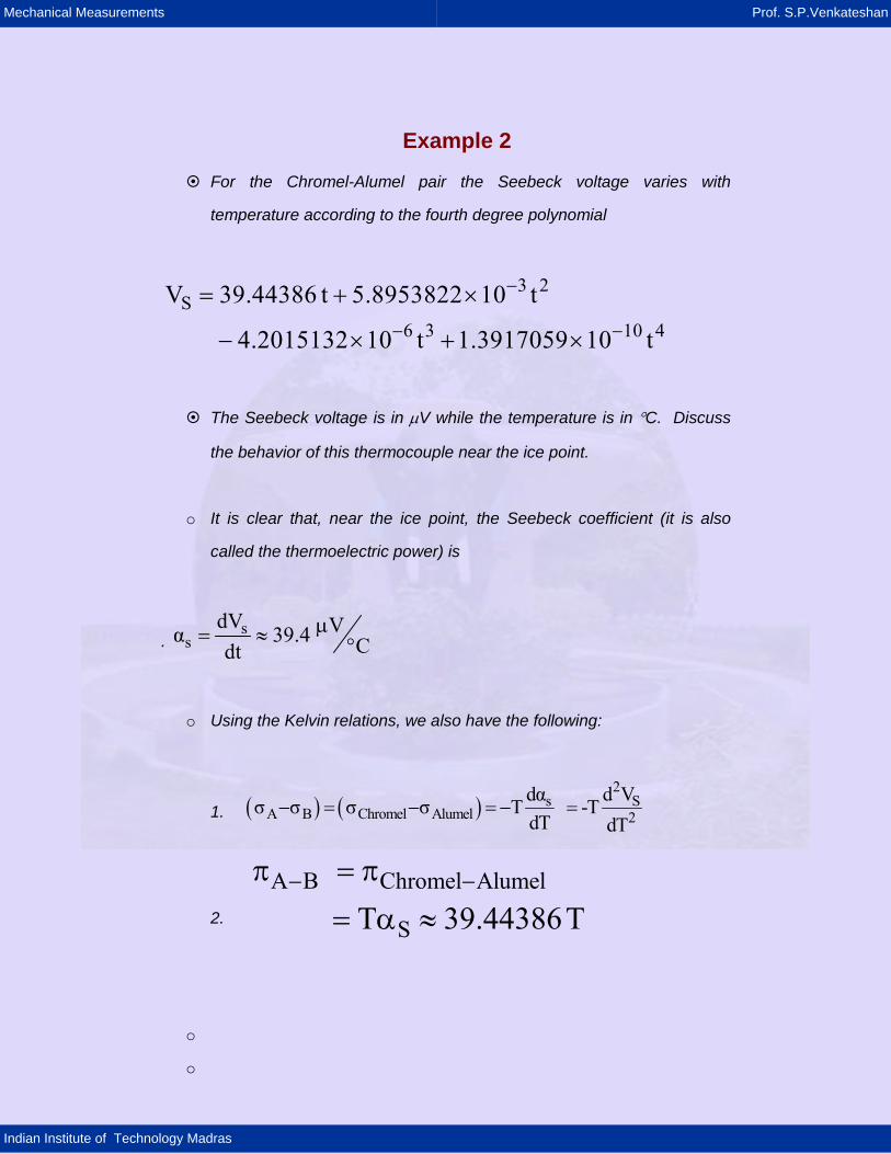
Example 2

For the Chromel-Alumel pair the Seebeck voltage varies with

temperature according to the fourth degree polynomial

3 2S

6 3 10 4

V 39.44386 t 5.8953822 10 t

4.2015132 10 t 1.3917059 10 t

−

− −

= + ×

− × + ×

The Seebeck voltage is in μV while the temperature is in °C. Discuss

the behavior of this thermocouple near the ice point.

o It is clear that, near the ice point, the Seebeck coefficient (it is also

called the thermoelectric power) is

. s

sdV Vα 39.4 Cdt

μ= ≈ °

o Using the Kelvin relations, we also have the following:

1. ( ) ( )2

s SA B Chromel Alumel 2

dα d Vσ σ σ σ T -T dT dT

− = − = − =

2.

A B Chromel Alumel

S

T 39.44386T

− −π = π

= α ≈

o

o



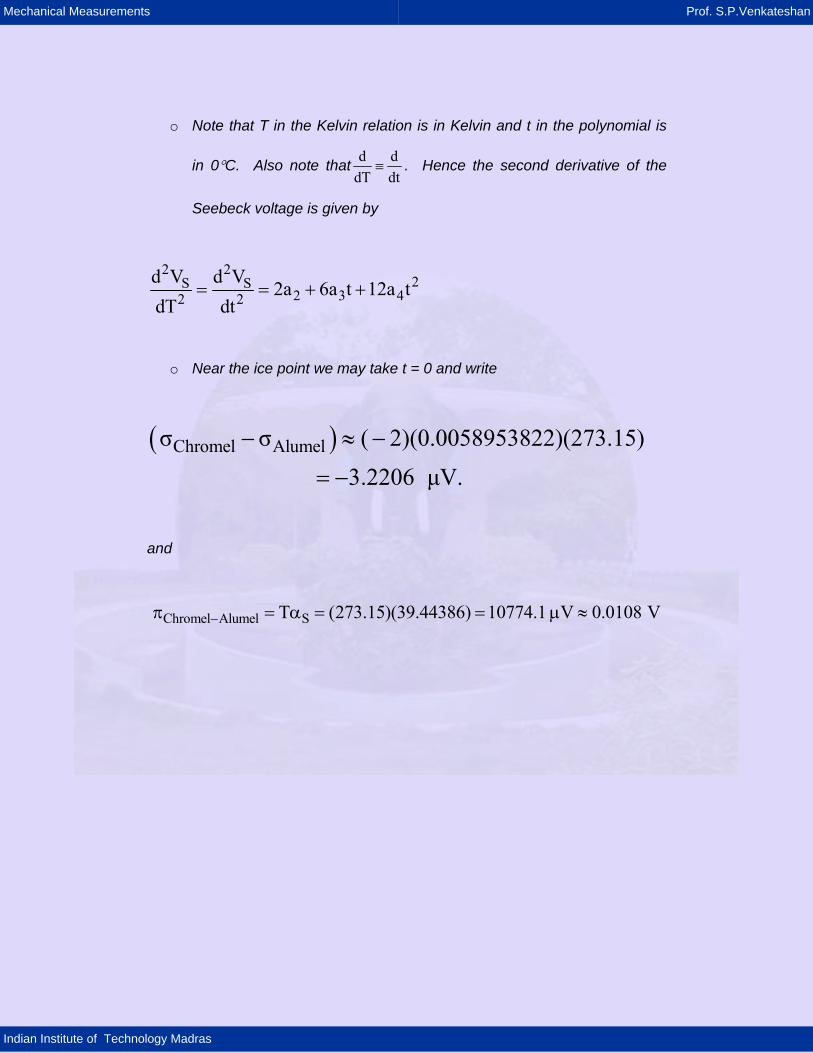
o Note that T in the Kelvin relation is in Kelvin and t in the polynomial is

in 0°C. Also note that d ddT dt

≡ . Hence the second derivative of the

Seebeck voltage is given by

2 22S S

2 3 42 2d V d V 2a 6a t 12a tdT dt

= = + +

o Near the ice point we may take t = 0 and write

( )Chromel Alumelσ σ ( 2)(0.0058953822)(273.15) 3.2206 μV.

− ≈ −

= −

and

Chromel Alumel ST (273.15)(39.44386) 10774.1 V 0.0108 V−π = α = = μ ≈



Example 3

The thermocouple response shown below (Copper Constantan

thermocouple with the cold junction at the ice point) follows the law VS

= a t + b t2. Obtain the parameters a and b by least squares. Here t is

in °C and VS is in mV.

Temperature, °C 37.8 93.3 148.9 204.4 260

VS, mV 1.518 3.967 6.647 9.523 12.572

o Since the fit follows the form specified above, it is equivalent to a linear

relation between E= VS/t and t. Since VS/t is a small number we shall

work with 100 VS/t and denote it as y. We shall denote the temperature

as x. The following table helps in evolving the desired linear fit.

x=t y=100VS/t x2 y2 xy yfit

37.8 4.015873 1428.84 16.12724 151.8 4.036073

93.3 4.251876 8704.89 18.07845 396.7 4.24048

148.9 4.46407 22171.21 19.92792 664.7 4.445255

204.4 4.659002 41779.36 21.7063 952.3 4.649661

260 4.835385 67600 23.38094 1257.2 4.854436

Sum: 744.4 22.22621 141684.3 99.22085 3422.7 6.638481

Mean = 148.88 4.445241 28336.86 19.84417 684.54 4.445181

(Note: I have used EXCEL to solve the problem)

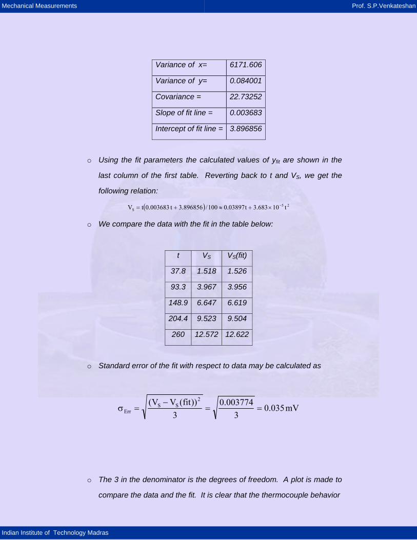
o The statistical parameters are calculated and presented in the form of a

table:



Variance of x= 6171.606

Variance of y= 0.084001

Covariance = 22.73252

Slope of fit line = 0.003683

Intercept of fit line = 3.896856

o Using the fit parameters the calculated values of yfit are shown in the

last column of the first table. Reverting back to t and VS, we get the

following relation:

( ) 25S t10683.3t03897.0100/3.896856t0.003683tV −×+≈+=

o We compare the data with the fit in the table below:

t VS VS(fit)

37.8 1.518 1.526

93.3 3.967 3.956

148.9 6.647 6.619

204.4 9.523 9.504

260 12.572 12.622

o Standard error of the fit with respect to data may be calculated as

mV035.03

003774.03

))fit(VV( 2SS

Err ==−

=σ

o The 3 in the denominator is the degrees of freedom. A plot is made to

compare the data and the fit. It is clear that the thermocouple behavior



is mildly nonlinear. The standard error of fir translates to approximately

±1°C!

o The inverse relation may similarly be obtained by fitting a linear relation

between S

tV

and SV . This is left as an exercise to the student. The

result obtained is 2S St 25.173V 0.3769V= − with a standard error

of t 2.209 Cσ = ± ° .

0

2

4

6

8

10

12

14

0 50 100 150 200 250 300Temperature oC

Seeb

eck

volta

ge m

VVS VS(fit)



Example 2 has shown that the thermoelectric data may be expressed in terms

of global polynomial to facilitate interpolation of data. A simple quadratic fit

has been used to bring home this idea. In practice the appropriate

interpolating polynomial may involve higher powers such that the standard

error is much smaller than what was obtained in Example 2. As an example,

the interpolating polynomial recommended for the K type thermocouple with

the reference junction at the ice point is given as:

-3 2 6 3

10 4

39.44386 t 5.8953822 10 4.2015132 10

+1.3917059 10SV t t

t

−

−

= + × − ×

×

This is a fourth degree polynomial and passes through the origin. The

Seebeck voltage is given in μV and the temperature is in °C. Using Kelvin

relations, the appropriate parameters are calculated near the ice point as:

39.444 /

273.15 39.44 = 10774.1

273.15 2 0.005895

= 3.22064

oss

AB S

SA B

dVV c

dtT

Vd

Tdt

V

= =

= = ×

− = − = × ×

−

α μ

π αμ

ασ σ

μ

The variation of the Seebeck coefficient over the range of this thermocouple is

given in Figure 7 below.



Figure 7 Variation of Seebeck coefficient with temperature

for K type thermocouple A short excerpt from a table of Seebeck voltages is taken and the

corresponding fit values as calculated using the above fourth degree

polynomial is given in Table 3. Note that the voltages in this table are in mV.

Table 3 comparison of actual data with fit

t VS VS(fit)

37.8 1.52 1.499 93.3 3.819 3.728 148.9 6.092 5.990 204.4 8.314 8.273 260 10.56 10.581

371.1 15.178 15.237 537.8 22.251 22.276 815.6 33.913 33.874

1093.3 44.856 44.879 1371.1 54.845 54.827

The maximum deviation is some 0.102 mV. The standard error is

approximately ±0.053 mV! This translates to roughly an error of ±1.2°C.

0

5

10

15

20

25

30

35

40

45

0 200 400 600 800 1000 1200 1400

Temperature oC

Seeb

eck

coef

ficie

nt μ

V/o C



The above shows that the three effects are related to the various terms in the

polynomial. The Seebeck coefficient and the Peltier coefficients are related to

the first derivative of the temperature. The contributions to the first derivative

from the higher degree terms are not too large and hence the Seebeck

coefficient is a very mild function of temperature. In the case of K type

thermocouple this variation is less than some 2% over the entire range of

temperatures. The Thomson effect is related to the second derivative of the

polynomial with respect to temperature. The value of this is again small and

varies from -3.22 �V at 0°C to a maximum value of +31.16 �V at 1350°C.

On the use of thermocouples for temperature measurement

We shall be looking at basic theoretical aspects and practical aspects of

measurement of temperatures using thermocouples. General ideas are

explored first followed by important practical aspects. Simple or basic

thermocouple circuit used for temperature measurement is shown in Fig. 8.

Figure 8 Simple thermocouple circuit The basic thermocouple circuit consists of a wire of P type material (P stands

for positive) and a wire of N type material (N stands for negative) forming a

measuring junction and a reference junction as shown (more about P and N

materials will be given later). The voltmeter is connected by making a break

P

N Ptm

tr

taV



in the P type wire as shown. Thus two more junctions are formed between P

type wires and connecting leads of the voltmeter. As we shall see later the

voltmeter will indicate the correct Seebeck voltage corresponding to tm if the

two extra junctions formed with the voltmeter are at the same temperature. If

m rt t , the voltmeter will indicate a positive voltage, the way it is connected.

We now look at the temperature variations along the wires that make up the

simple circuit shown in Fig. 8. It is likely that the thermocouple wires pass

through a region of uniform temperature (eg. the laboratory space) a short

distance away from the junctions that are maintained at the indicated

temperatures. The state of affairs is schematically shown in Fig. 9. It is clear

that the temperature varies significantly within a short distance from the

measuring and reference junctions (the variation is determined by the thermal

properties of the wire and the nature of the ambient) and comes to the

ambient temperature. Recall that the thermoelectric effects (Peltier and

Thomson) are confined to either the junctions or to the region along the wires

that have a temperature variation along them. Those regions along the wire

that are isothermal do not give rise to any thermoelectric effects. Hence it is

possible to change the simple circuit shown in Fig. 8 to a practical circuit

shown in Fig. 10.

In the practical circuit the thermocouple wires are long enough to see that the

end away from the junctions is at the room temperature. Copper wires are

used as shown in the largely isothermal region. Apart from the measuring

and the reference junctions there are six more junctions that are formed!



Figure 9 Temperature variations along the wires

Figure 10 Practical thermocouple circuit

We shall now look at these junctions in the light of three laws of thermoelectric

circuits that are discussed below.

Laws of thermoelectric circuits

I. Law of homogenous materials

A thermoelectric current cannot be sustained in a circuit of a

single homogenous material however it varies in cross section by the

application of heat alone

II. Law of intermediate materials

PN

P

N

tm

ta

tr

t

Cu

Cu Cu VP

NP

tm

N

tr

ta



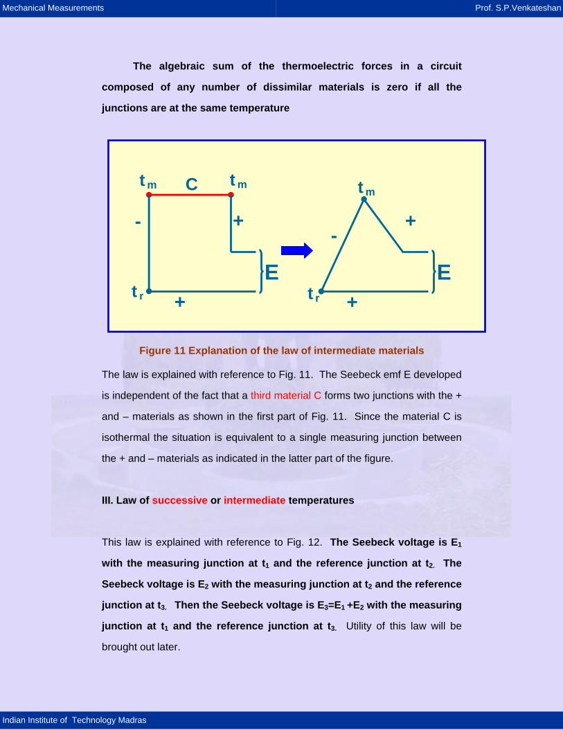
The algebraic sum of the thermoelectric forces in a circuit

composed of any number of dissimilar materials is zero if all the

junctions are at the same temperature

Figure 11 Explanation of the law of intermediate materials

The law is explained with reference to Fig. 11. The Seebeck emf E developed

is independent of the fact that a third material C forms two junctions with the +

and – materials as shown in the first part of Fig. 11. Since the material C is

isothermal the situation is equivalent to a single measuring junction between

the + and – materials as indicated in the latter part of the figure.

III. Law of successive or intermediate temperatures

This law is explained with reference to Fig. 12. The Seebeck voltage is E1

with the measuring junction at t1 and the reference junction at t2. The

Seebeck voltage is E2 with the measuring junction at t2 and the reference

junction at t3. Then the Seebeck voltage is E3=E1 +E2 with the measuring

junction at t1 and the reference junction at t3. Utility of this law will be

brought out later.

+

+

-

C

E

tm tm

tr

+

+

-

E

tm

tr



Now we get back to the practical thermocouple circuit shown in Fig. 10. The

six extra junctions that are formed are all at a uniform temperature equal to

the ambient temperature. The laws of thermoelectricity enunciated above

guarantee that these do not have any effect on the Seebeck voltage

developed by the thermocouple circuit. The copper wires are at room

temperature (uniform temperature) and hence the law of intermediate

materials asserts that the circuit is equivalent to one in which the copper wire

is absent! In fact the temperature variations along the wires are as indicted in

Fig. 13. The reason for the use of copper lead wires is to cut down on the

cost of expensive thermocouple wires. Sometimes compensating lead wires

are made use of. These are made of the same material as the thermocouple

wires but not of the same high quality. They may also be made of cheaper

alloys that have thermoelectric properties closely following the thermoelectric

properties of the thermocouple wires themselves.

Figure 12 Explanation of the law of intermediate temperatures

t1

E1

t2 t2

E2

t3

t1

E3

t3

+

=

=E1+E2



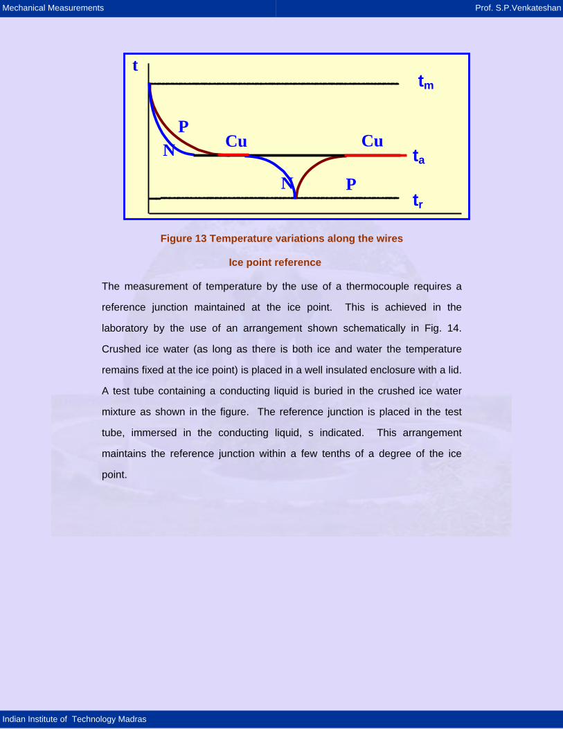
Figure 13 Temperature variations along the wires

Ice point reference The measurement of temperature by the use of a thermocouple requires a

reference junction maintained at the ice point. This is achieved in the

laboratory by the use of an arrangement shown schematically in Fig. 14.

Crushed ice water (as long as there is both ice and water the temperature

remains fixed at the ice point) is placed in a well insulated enclosure with a lid.

A test tube containing a conducting liquid is buried in the crushed ice water

mixture as shown in the figure. The reference junction is placed in the test

tube, immersed in the conducting liquid, s indicated. This arrangement

maintains the reference junction within a few tenths of a degree of the ice

point.

Cu

t

P

N P

N

Cu

tm

tr

ta



Figure 14 Ice point reference junction

It is seldom that individual ice point references are maintained while using

several thermocouples for measuring temperatures at different points in an

apparatus. The laws of thermoelectricity come to our help in designing a

suitable arrangement with selector switch and a single ice point reference

junction as shown in Fig. 15.

Figure 15 Many measuring junctions with a single reference junction

Reference Junction

Conducting Medium

Crushed Ice Water Mixture

Thermocouple Wires

Insulated Vessel (Thermos Flask)

Stopper

V 3

1

2

4

Ice point

Selector switch

+

+

+

+

-

-

-

-

Cu Cu

Cu

- +

Junction Box



The switch is generally a rotary switch with gold plated contacts. Switches

are available with a capacity of 8, 16 or 32 thermocouple connections. The

switch is a double pole single throw type that will connect each thermocouple

pair to complete the circuit with the voltmeter and the cold junction.

Use of thermocouple tables

Practical aspects of thermoelectric thermometry

Even though, in principle, one can use any two dissimilar materials as

candidates for constructing thermocouples thermometry demands that there

be standardization so that one may use with very little effort. Also no single

thermoelectric thermometer can cover the wide range of temperatures met

with in practice. The materials chosen must be available easily from

manufacturers with guaranteed quality. In view of these only a few

combinations of materials are made use of in day to day laboratory practice.

The common thermocouple materials are shown in Table 4. The entries in

the table are such that all the materials that are below the one under

consideration are negative with respect to it. This means that the

thermoelectric power increases as the row count between two materials

increases. The Seebeck voltages of materials are measured with respect to

Platinum 67 (the platinum standard used by the National Institute of

Standards and Technology – NIST - USA) as the standard second element.

The columns correspond to the usable temperature ranges for the materials.

Several of the materials are alloys and they are sold under trade mark. Law

of intermediate materials is invoked to combine the thermoelectric data of two

materials that are individually measured with Platinum 67 as the reference

material.



Table 4 Common thermocouple materials

100°C 500°C 900°C Antimony Chromel Chromel Chromel Nichrome Nichrome Iron Copper Silver Nichrome Silver Gold Copper Gold Iron Silver Iron Pt90Rh10 Pt87Rh13 Pt90Rh10 Pt Pt Pt Cobalt Palladium Cobalt Alumel Cobalt Palladium Nickel Alumel Alumel Palladium Nickel Nickel ConstantanConstantan Constantan Copel Copel Bismuth

Presumably Seebeck was experimenting with Antimony and Bismuth when he

discovered thermoelectricity. It appears that he had hit upon materials with

the largest thermoelectric power! If the candidate thermocouple material is

positive with respect to Platinum 67 the Seebeck voltage will be positive

across the candidate – Platinum 67 terminals. In general, if a candidate

material is positive with respect to a second material the Seebeck voltage will

be positive across the candidate and the second material terminals.

Table 5 Standard thermocouple types

Type + / - Wires +/- Color

B Pt94%Rh6% / Pt Grey / Red E Chromel / Constantan Purple / Red J Iron / Constantan WWWhhhiiittteee / Red K Chromel / Alumel YYYeeellllllooowww / Red R Pt87%Rh13% / Pt Black / Red S Pt90%Rh10% / Pt Black / Red T Copper / Constantan Blue / Red



Table 6 Typical thermocouple reference table From: http://www.temperatures.com/tctables.html

ITS90 Table for Type K thermocouples �C 0 1 2 3 4 5 6 7 8 9 10 Thermoelectric voltage in mV

0 0 0.039 0.079 0.119 0.158 0.198 0.238 0.277 0.317 0.357 0.397 10 0.397 0.437 0.477 0.517 0.557 0.597 0.637 0.677 0.718 0.758 0.798 20 0.798 0.838 0.879 0.919 0.96 1 1.041 1.081 1.122 1.163 1.203 30 1.203 1.244 1.285 1.326 1.366 1.407 1.448 1.489 1.53 1.571 1.612 40 1.612 1.653 1.694 1.735 1.776 1.817 1.858 1.899 1.941 1.982 2.023

50 2.023 2.064 2.106 2.147 2.188 2.23 2.271 2.312 2.354 2.395 2.436 60 2.436 2.478 2.519 2.561 2.602 2.644 2.685 2.727 2.768 2.81 2.851 70 2.851 2.893 2.934 2.976 3.017 3.059 3.1 3.142 3.184 3.225 3.267 80 3.267 3.308 3.35 3.391 3.433 3.474 3.516 3.557 3.599 3.64 3.682 90 3.682 3.723 3.765 3.806 3.848 3.889 3.931 3.972 4.013 4.055 4.096

100 4.096 4.138 4.179 4.22 4.262 4.303 4.344 4.385 4.427 4.468 4.509 110 4.509 4.55 4.591 4.633 4.674 4.715 4.756 4.797 4.838 4.879 4.92 120 4.92 4.961 5.002 5.043 5.084 5.124 5.165 5.206 5.247 5.288 5.328 130 5.328 5.369 5.41 5.45 5.491 5.532 5.572 5.613 5.653 5.694 5.735 140 5.735 5.775 5.815 5.856 5.896 5.937 5.977 6.017 6.058 6.098 6.138

Not all combinations of materials given in Table 4 are used in practice. A

small number of them (Table 5) are used and are available from reputed

manufacturers. Also the thermoelectric data are available in the form of

tables for each of these. As an example Table 6 shows an excerpt of the

table appropriate for K type (Chromel is the positive element and Alumel is the

negative element) thermocouple. The table assumes that the reference

junction is maintained at the ice point.

Some interesting things may be noted by examining the table. The Seebeck

coefficient for K type thermocouple is approximately 40 μV/°C. If we use a

voltmeter that can resolve 0.01 mV or 10 μV the temperature resolution is

about 0.25°C! Even this is in not achieved in practice. Voltmeters capable of

such high resolution are expensive and hence it is not possible to achieve sub

degree resolution levels in ordinary laboratory practice. The accuracy limits

that are possible to achieve are given in Table 7 for various thermocouple

pairs.



Table 7 Accuracy and range values of some thermocouple sensors

Thermocouple Full range °C

Accuracy °C or %

Range °C ISA* standard limits

Chromel Alumel, K Type

-185 to 1371 ±2°C

±0.75%

-18 to 277 277 to 1371

Iron – Constantan, J Type -190 to 760 ±2°C ±0.75%

-18 to 277 277 to 760

Copper – Constantan, T Type

-190 to 400 ±2% ±0.8°C ±0.75%

-190 to –60 -60 to 93 93 to 370

Pt90Rh10-Pt, S Type

0 to 1760 ±2.8°C ±0.5%

0 to 538 538 to 1482

W – W74Rh26 W95Rh5-W74Rh26

0 to 2870 ±4.5°C ±1%

0 to 427 427 to 2870

*ISA stands for Instrument Society of America Note that Tungsten - Tungsten Rhenium thermocouples (special but

expensive thermocouples) are useful for the measurement of very high

temperatures normally inaccessible to other thermocouples. However the

accuracy limits are not as good as for the other thermocouples

The useful ranges of thermocouples are determined, (a) by the thermoelectric

behavior and (b) by the physical properties of the wire materials, as the

temperature is changed. At elevated temperatures the integrity of the

thermocouple wire materials as well as the junction is important. The

materials of the wires are also prone to thermal fatigue when the junctions are

subjected to thermal cycling during use. In view of the fact that the materials

near the junctions experience these thermal cycles it is possible to discard a

small length close to the junction and remake a junction for subsequent use.

Materials also age during use and may have to be discarded if the

thermoelectric properties change excessively during use.

To round of this discussion we present (Fig. 16) the thermoelectric output of a

K type thermocouple over the range of its usefulness. We notice that over an



extended range the output is non-linear. Note that this pair of materials is far

apart in Table 1. Hence the thermoelectric power is very large and next only

to J type (Iron – Constantan) thermocouple. The sensitivity also compares

favorably with T type (Copper – Constantan) thermocouple. Even though

these three types have high sensitivity the ranges are different. K type has

the widest range among these three types. Both K type and T type

thermocouples are commonly used in laboratory and industrial applications.

Iron is prone to corrosion and hence is of limited use.

0

10

20

30

40

50

60

0 200 400 600 800 1000 1200 1400

t,oC

V S, m

V

Figure 16 Seebeck volts – temperature relationship for K type thermocouple

Insulation systems Thermocouples are made with wires of various diameters according to

requirement. The P and N wires are expected to not contact each other

(electrically) excepting at the junctions. Hence it is necessary to cover the

wire with an electrical insulator. It is normal for the P and N wires to be

individually covered with insulation, the two wires laid parallel to each other

and covered with an outer sheath encasing both the wires. The insulation



material is chosen with the temperature range in mind. A list of insulation

materials along with the useful range of temperatures is given in Table 8.

Table 8 Thermocouple insulation systems

Insulation Temperature

limits oC Nylon -40 to 160 PVC -40 to 105 Enamel Up to 107 Cotton over enamel Up to 107 Silicone rubber over Fiberglass -40 to 232 Teflon and Fiberglass -120 to 250 Asbestos -78 to 650 Tempered Fiberglass Up to 650 Refrasil® Up to 1083

Sometimes the thermocouple is protected from mechanical damage by a

protective tube. The protective tube material is again chosen based on the

temperature range and the ruggedness desired.

Table 9 Ceramic protecting tube materials

Material Composition Max. Temp.oC Quatrtz Fused Silica 1260 Siliramic® Silica-Alumina 1650 Durax® Silicon Carbide 1650 Refrax® Silicon Nitride Bonded Silicon Carbide 1735 Alumina 99% Pure 1870

Some of the materials shown in tables 8 and 9 are proprietary in nature and

are identified by the trade name. Some times the protective tube material

may be made of metal like stainless steel. Since metals are good conductors

of electricity the insulation of the individual wires must be adequate to avoid

any electrical contact with the protective metal tube.

Thermocouple junctions Thermocouple junctions may be formed by various means. The most

common method is to weld or fuse the two materials to form a junction.

Welding is commonly made by twisting the two wires for a short length,



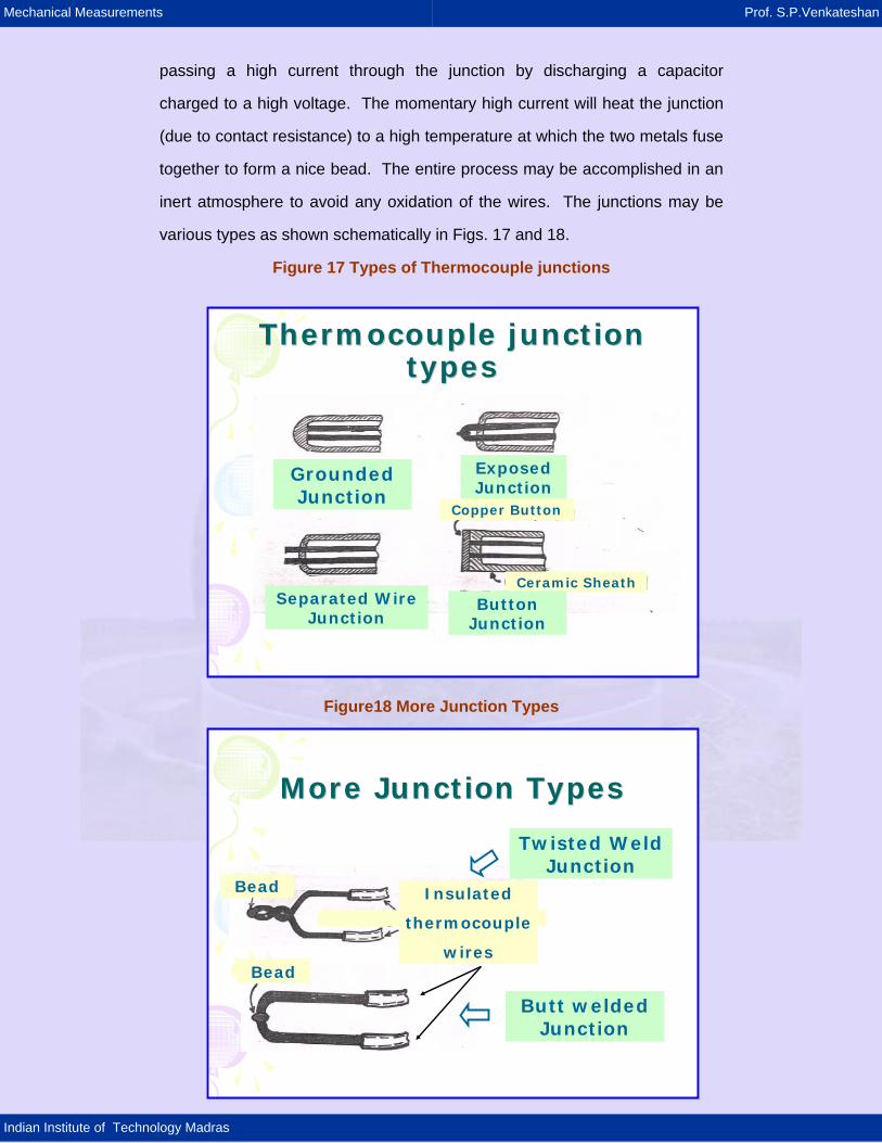
passing a high current through the junction by discharging a capacitor

charged to a high voltage. The momentary high current will heat the junction

(due to contact resistance) to a high temperature at which the two metals fuse

together to form a nice bead. The entire process may be accomplished in an

inert atmosphere to avoid any oxidation of the wires. The junctions may be

various types as shown schematically in Figs. 17 and 18.

Figure 17 Types of Thermocouple junctions

Figure18 More Junction Types

13

Thermocouple junction Thermocouple junction typestypes

Grounded Junction

Exposed Junction

Separated Wire Junction

Copper Button

Ceramic Sheath

Button Junction

14

More Junction TypesMore Junction Types

Bead

Bead

Insulated

thermocouple

wires

Butt welded Junction

Twisted Weld Junction



Grounded junction: Such a junction is used (Fig. 17) if one wants avoid direct

contact between the thermocouple bead and the process fluid. The protective

tube provides a barrier between the junction and the process fluid. This type

of arrangement increases the response time of the thermocouple when

measuring temperature transients.

Exposed junction: This arrangement (Fig. 17) is acceptable if the process

space does not adversely affect the thermocouple materials. This type of

arrangement decreases the response time of the thermocouple when

measuring temperature transients.

Separated wire junction: The two wires are allowed to float within the process

space as shown in Fig. 17. The process fluid (molten metal in metallurgical

applications) provides the electrical connection between the P and N wires.

Button junction: The P and N wires are attached to a copper (high

conductivity material) button such that the thermal contact between the

process fluid (may be gas like air) and the junction is enhanced. This is

beneficial from the response time point of view as well as from the

thermometric error point of view (as we shall see later).

Junctions may be made by twisting the P and N wires together. Twisting

action itself cold works the two materials to form good contact. In addition the

two wires may also be welded as shown in Fig. 18. The junction may also be

formed by butt welding the two wires as shown in Fig. 18.



Figure 19 Bayonet or pencil type of thermocouple probe

Sometimes a thermocouple probe is constructed in the form of a bayonet or

pencil as indicated in Fig. 19. The figure shows a J type thermocouple probe

with the protective tube of Iron (P type material) and a wire of constantan (N

type material) attached to the bottom of the tube with fiberglass insulation

between the two. The connections to the external circuit are made through

terminal blocks.

““Bayonet” or “Pencil” Bayonet” or “Pencil” TypeType

Terminal Block

Fiberglass

Insulation

Constantan Wire

Iron Tube



Thermocouples in series and parallel Differential thermocouple:

Figure 20 Differential thermocouple for the direct

measurement of temperature difference Thermocouples may be used in other ways than the ones described earlier.

The temperature difference between two locations in a process may be

obtained by measuring the two temperatures individually using two separate

thermocouples and then taking the difference. The errors involved in each

such measurement will propagate and give an overall error that may be

unacceptable in practice. A way out of this is to use the differential

thermocouple (this is just the basic thermocouple circuit with the hot and cold

junctions at different temperatures!) and measure the temperature difference

directly once ΔVS is measured. In applications where the temperature

difference to be measured is small, we obtain the temperature difference

directly as S

SVt

αΔ

=Δ where a constant value of Sα appropriate to the chosen

thermocouple pair may be used. It is even possible to amplify the output

using a high gain low noise amplifier to improve the measurement process.

The differential thermocouple arrangement may also be used as a calibration

arrangement. If 21 tt = , the differential thermocouple should give zero voltage

output, if the two thermocouples are of the same type and behave alike. If we

choose one of the thermocouples to be a standard calibrated one, the other

ΔVS

t1

t2

-

-

+

+



the thermocouple is one to be calibrated, and both are of the same type it is

easy to arrange both the junctions to be subjected to the same temperature.

The non-zero output, if any, gives the error of one thermocouple against the

other. The temperature itself may be measured independently using a

standard thermocouple so that we can have a calibration chart giving the

thermocouple error as a function of temperature.

The amplification may also be accomplished by using several junctions in

series as shown in Fig. 21. This arrangement is referred as a thermopile and

produces an output that is n times the value with a single differential

thermocouple where n is the total number of hot or cold junctions. In the

example shown the thermopile is being used as a radiation flux sensor. The

shading ring prevents illumination of the cold junctions and thus produces a

number of differential thermocouples in series.

Figure 21 Several differential thermocouples in series forming a thermopile

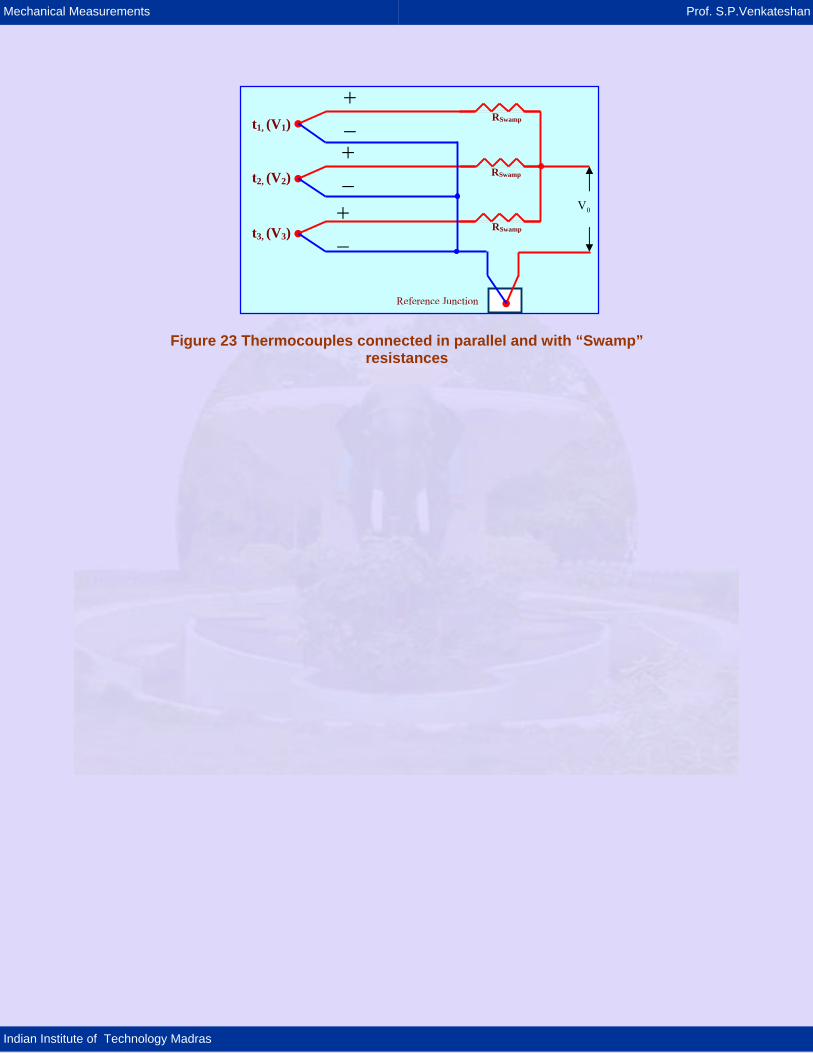
Thermocouples in parallel: In practice we may require the average temperature in a region where the

temperature may vary. One way of doing this would be to measure all the

temperatures individually with separate thermocouples and then take the

mean. However, it is possible to measure the mean value directly using

ο Illuminated Junctions

V

• Shaded Junctions

Shading ring



several thermocouples connected in parallel as shown in Fig. 22. The

thermoelectric output corresponding to the junctions are as indicated in the

figure and these correspond to the respective measuring junction

temperatures. Assuming that all the thermocouples are identical, the output

voltage is given by

3

VVVV 3210

++= (1)

Thus the inferred temperature is the mean of the measuring junction

temperatures. The accurate averaging of the Seebeck voltages relies on

each thermocouple's wire resistances being equal. If this is difficult to achieve

one may use equal but large (large compared to the resistance of the

thermocouple wires) “swamping” resistance in each circuit to alleviate the

problem. This is indicated in Fig. 23.

Figure 22 Thermocouples connected in parallel

t3, (V3)

t1, (V1) −+

0V−+

−+

t2, (V2)

Reference Junction



Figure 23 Thermocouples connected in parallel and with “Swamp”

resistances

t3, (V3)

t1, (V1) −+

0V−+

−+

t2, (V2)

Reference Junction

RSwamp

RSwamp

RSwamp



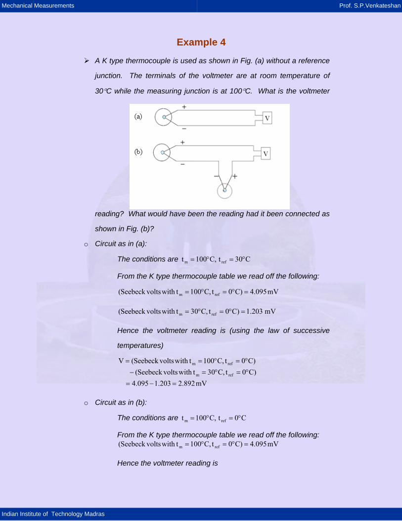
Example 4

A K type thermocouple is used as shown in Fig. (a) without a reference

junction. The terminals of the voltmeter are at room temperature of

30°C while the measuring junction is at 100°C. What is the voltmeter

reading? What would have been the reading had it been connected as

shown in Fig. (b)?

o Circuit as in (a):

The conditions are C30t,C100t refm °=°=

From the K type thermocouple table we read off the following:

mV095.4)C0t,C100twithvoltsSeebeck( refm =°=°=

mV203.1)C0t,C30twithvoltsSeebeck( refm =°=°= Hence the voltmeter reading is (using the law of successive

temperatures)

mV892.2203.1095.4)C0t,C30twithvoltsSeebeck()C0t,C100twithvoltsSeebeck(V

refm

refm

=−=°=°=−°=°==

o Circuit as in (b):

The conditions are C0t,C100t refm °=°=

From the K type thermocouple table we read off the following: mV095.4)C0t,C100twithvoltsSeebeck( refm =°=°=

Hence the voltmeter reading is



mV095.4)C0t,C100twithvoltsSeebeck(V refm

=°=°==

Example 5

Consider the thermopile arrangement shown in the figure. What will be

the output voltage?

o Three materials are used in the circuit. KP and KN at the measuring

temperature of 100°C form four junctions. There are three cold

junctions between KN and KP at 30°C. There is one junction each

between KP – Cu and KN – Cu. Since these two junctions are at the

same temperature, the law of intermediate temperatures says that

these two junctions are equivalent to a single junction between KN and

KP at 30°C. Thus effectively there are four cold junctions.

o Thus the voltage indicated will be four times that due to a measuring

junction at 100°C and a reference junction at 30°C. By the law of

intermediate temperatures, we thus have:

KN KP Cu

All junctions at 100°C

All junctions at 30°C

V



[ ]( )( )

( ) mV11.568892.24203.1095.44C0andC30betweenSeebeck

C0andC100betweenSeebeck4

C30andC100betweenSeebeck4V

=×=−×=

⎥⎦

⎤⎢⎣

⎡°°−°°

×=

°°×=



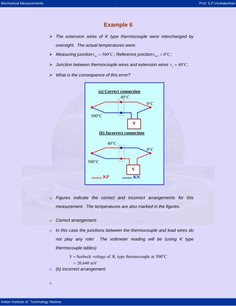
Example 6

The extension wires of K type thermocouple were interchanged by

oversight. The actual temperatures were:

Measuring junction C500t m °= ; Reference junction C0t ref °= ;

Junction between thermocouple wires and extension wires C40t j °= .

What is the consequence of this error?

o Figures indicate the correct and incorrect arrangements for this

measurement. The temperatures are also marked in the figures.

o Correct arrangement:

o In this case the junctions between the thermocouple and lead wires do

not play any role! The voltmeter reading will be (using K type

thermocouple tables)

mV640.20C500atlethermocouptypeKofvoltageSeebeckV

=°=

o (b) Incorrect arrangement:

o

(a) Correct connection

(b) Incorrect connection

0°C 40°C

500°C

V

0°C 40°C

500°C

V

KP KN



o In this case there are effectively four junctions. The net voltage

indicated is given by

C40C0C40C500 VVVVV °°°° −+−=

o The notation used is

C0junctionatreferenceandCtatjunctionmeasuringwithvoltageSeebeckV Ct °°=°

o Using K type thermocouple tables we get

mV418.17611.10611.1640.20V =−+−=

o If one were to convert this to a temperature based on the assumption

that the measuring junction and reference junction are correctly

connected, the temperature would be (using K type thermocouple

tables) C2.424t °= . Thus the consequence of the mistake is that the

temperature is underestimated by 74.8°C.

Documents

Sub Module 2.2 Thermoelectric thermometry