Sub-Modelling Boundary Element approach for stress concentration · PDF fileSub-Modelling Boundary Element approach for stress concentration in samples exposed to pitting corrosion

Sub-Modelling Boundary Element approach for stress concentration in samples exposed to pitting corrosion

A. Peratta & C. Brebbia Wessex Institute of Technology, UK

Abstract

The paper presents a Sub-Modelling - Boundary Element Method (BEM) for computing SCFs in samples exposed to pitting corrosion. The goal of this technique is to provide a detailed mapping of the stress concentration factor (SCF) including the effects of deep pits of several microns in a sample of a few centimetres size, provided that the topographical data of the sample is known in detail. The methodology is summarised as follows. First, the original geometrical data representing the top surface of the sample is used for building a hierarchical sequence of defeatured levels by means of a moving average approach. Second, an iterative three-dimensional BEM solving scheme is launched in order to explore and solve the sample data at a defeatured level. The calculation resolution level can be selected by the user. When the iterative solving scheme ends, an iterative assembly scheme starts in which the results of SCF and the geometrical error of the model are collocated at sampling points corresponding to the resolution selected by the user. Finally, and repeatedly if necessary, a new solving iteration sequence may be launched with increased resolution, in the regions of the sample data that require more accuracy, such as zones of high SCF, large geometrical error, or steep gradient of any of them. The process continues until convergence of results is achieved. The tool has been successfully tested in several real case scenarios, and the results obtained compare well with experimental findings. Keywords: pitting corrosion, stress concentration, Boundary Element Method, Sub-Modelling.

© 2007 WIT PressWIT Transactions on Engineering Sciences, Vol 54, www.witpress.com, ISSN 1743-3533 (on-line)

Simulation of Electrochemical Processes II 277

doi:10.2495/ECOR070271

1 Introduction

One of the most damaging and prevalent types of corrosive attack most likely to breach a metallic structure under stress is localized corrosion [1]. Pitting is a form of corrosion in metals characterised by its extremely local damaging effect. Pitting corrosion is characterised by having the anodic and cathode areas, in close vicinity to each other. The former has poor access to oxygen in the electrolyte, while the latter appears in areas in contact with high concentration of oxygen. Hence, pitting can be regarded as a special case of galvanic corrosion, in which the anode and cathode are extremely close to each other. With time, the corrosion area tends to dig into the un-corroded metal, and further increase the local lack of oxygen in the anode. Pitting corrosion usually leads to the creation of small and deep holes of sub-millimetric diameter in the exposed metallic surface. It is supposed that gravity effects contribute to the process. The structural damage induced by pitting is difficult to appreciate by simple visual inspection. Moreover, when the metallic structure is subject to mechanical stress, the holes induced by pitting can amplify the local stress concentration in factors ranging from two to five. Finally, pits originate cracks which will end up damaging the structure. It is well known that pitting can also be initiated by surface defects and heterogeneities in the metal. Either a scratch or a local change in composition can cause pitting. In addition, homogeneous surfaces and metals characterised by uniform corrosion such as mild steels are less prone to pitting. In opposition, materials more resistant to uniform corrosion such as stainless steels, nickel and aluminium alloys are more susceptible to pitting. The study of SCFs induced by pitting is motivated by the lack of low cost/efficient-ratio methods available nowadays for detecting and predicting the damage in industrial environments. There have been a number of reviews of theories and mechanisms for describing pitting and crevice corrosion [1-3]. A thorough revision of the theoretical conceptual models for describing pitting corrosion has been done in ref. [4]. Detailed modelling of fatigue crack corrosion and crack initiation due to pitting has been studied with the Finite Element Method (FEM) in [5,6]. The need to retain in service expensive and large maritime structures beyond their lifetime expectations has triggered a significant number of research activities towards the prediction and risk assessment, where probabilistic approaches have recently proven quite useful [7]. The aim of this paper is to present a computer simulation tool that has been developed in order to assess the SCF of metallic samples exposed to pitting for which exact topography is known in detail, i.e. by scanning microscopy techniques. The characteristic size of a sample may be of few centimetres while the characteristic length of the dangerous pits in the sample might be of few tens of microns or microns. The conceptual model for the numerical test is illustrated in Fig. 1.


278 Simulation of Electrochemical Processes II

Figure 1: Conceptual model for the numerical test showing a sample with pitting defects exposed to lateral unitary stress along y direction.

The sample of characteristic size L and thickness H is constrained to lateral unitary stress T in y direction. The top surface of the sample may include a significant number of pits with characteristic diameter D and depth h. The stress analysis is conducted by means of BEASY Mechanical Design module [8], a three dimensional computer code based on the Boundary Element Method (BEM) [9]. The key advantages of the BEM are first that it is based on the fundamental solution of the leading differential equation, and second that it does not need domain discretisation, i.e. in three dimensional models the computational mesh is required in the boundary only. One of the major complications in BEM is that it yields fully populated unsymmetric linear systems of equations, and when the number of degrees of freedom becomes too large the calculation becomes prohibitive. Roughly speaking, a few tens of thousands degrees of freedom (i.e. 50000) may require a storage of few gigabytes (10 GBytes) in full format and could take a couple of days to run in a Pentium IV PC with 3GHz using a standard direct Gaussian solver. Noteworthy, the accuracy achieved with 50000 degrees of freedom is usually superior than the one obtained with other standard methods such as FEM, distributing the same amount of degrees of freedom in volume. To illustrate the motivation of this approach, consider a problem in which a sample of L ~ 100mm with a significantly large number of pits of average size D~10µm randomly distributed is laterally loaded with constant stress. The challenge is to determine the stress concentration field defined as:



TS

SCF yy= (1)

In order to take into account the pits with a reasonable accuracy, it is necessary to use at least a 2 µm sampling resolution for the top surface. Henceforth, the top surface alone will produce a mesh of with 92.5 10× nodes. This figure yields a prohibitively large number of degrees of freedom, even unpractical for a supercomputer. On the other hand, it can be demonstrated that the stress field is a very local effect. If pits are separated by more than 5D, they can be considered as uncorrelated. This behaviour helps to decompose the large problem into smaller ones by means of a sub-modelling approach. A possible sub-modelling approach would be to solve 1000000 sub-models of 0.1mm by 0.1mm, covering the whole surface, where each one of them accounts for 2500 degrees of freedom. Models of few thousand degrees of freedom can be solved in a matter of seconds in an average PC. Then, roughly speaking, with a small cluster of four to eight PC’s the complete problem can be solved within few days. The method above outlined can be substantially improved if we start solving the problem in a rather defeatured geometry with few sub-models, and successively refined sub-modelling stages are applied in an iterative way in combination an adaptive mesh refinement that improves the resolution only in the regions where high SCFs are being discovered. This is the main idea implemented in the present work. The paper is organised as follows. Section 2 outlines the technical implementation of the described approach. Section 3 provides basic guidelines on how to choose a safe sub-modelling approach. A case study is that briefly illustrates the applicability of the method is presented in section 4, and finally the corresponding conclusions are elaborated in Section 5.

2 Iterative solving scheme Figure 2 shows the general sub-modelling approach with three calculation stages. Each rectangle represents a sub-model, characterised by certain space resolution and size. Both size and resolution of the sub-model should be chosen according to the results of the SCF obtained in the previous stage. The initial input consists of the original large sample with detailed geometrical information. In the first stage, the original sample is decomposed into N1 sub-models with coarser resolution. The density of the hatch pattern represents the mesh resolution of the associated sub-model. Stage 2 (with N2 sub-models) performs another division to the previous iteration with increased space resolution. Stage 3 increases the number of sub-models but the mesh resolution is refined only in those sub-models which presented high concentration factor in the previous step. The number of stages may continue until the desired level of resolution and geometrical accuracy is achieved. At the end of the process, the pits with higher SCF will have been identified and solved. In some cases, the boundary conditions between sub-models must be readjusted iteratively, hence the method will iterate between two stages until the boundary conditions are properly adapted, same as in a standard multi-grid approach.



Original sample

Stage1

Stage2

Stage3

Figure 2: Illustrative sketch showing different stages of the iterative sub-modelling approach. Each cell represents a sub-model, the density of the hatched area represents the space resolution of the computational grid.

The iterative solving scheme operates in the following way. An initial representation of the top surface, usually coarser than the original data, is used to automatically create a NurbSurface model by the geometry modeller BEASY-GiD [10]. Then, a parametric wireframe structure is connected to the created Nurb-surface in order to build a three-dimensional sub-model of the corroded surface. The remaining wireframe is then filled with flat surfaces to define a closed six-faced volume [8]. Next BEASY-GiD [8] creates a computational grid of the 3D model with the resolution and quality chosen either by the user or automatically by the software in a configuration file. Since BEASY is based on the Boundary Element Method, the computational grid is created only for the surface of the sub-model, thus avoiding meshing the volume. This represents an important advantage which helps to speed up model generation and further calculation time. Once the model is created by BEASY-GiD, the information is passed as input to the BEASY MECHANICAL DESIGN software which conducts the stress analysis. As output, BEASY provides the stress and strain tensors results in all points of the boundary mesh of the sub-model. BEASY results of each sub-model are stored in a file for later assembly into the appropriate location of the overall result file. The solving iterations stop once all the sub-models are completed. The above mentioned tasks are automatically performed in non-interactive mode, so as to



avoid time consuming graphical interactions during the iteration over a large number of sub-models.

3 Sub-modelling

In each iteration stage a certain number of sub-models are solved after suitable space resolution and dimensions are chosen for them. A 3D mesh with boundary conditions is associated to each sub-model. The top surface of each sub-model undergoes three approximations. The first one happens when defeaturing the original sampled data with a moving average filter, the second one is introduced when representing the topography of the defeatured data with a rectangular grid and Nurb-Surfaces, and the third approximation occurs when meshing the surface approximated by Nurb-surfaces with a computational grid made of either linear (flat) or quadratic (curved) elements. The accuracy at each level of approximation can be adjusted according to the quality of results sought by the user. We consider the original sample as a parallelepiped with L >> H. All sub-models in any stage will be also parallelepipeds of size hww ×× . In order to decrease the computational burden the number of the degrees of freedom (NDOF) of the sub-models should be as small as possible. For a fixed space resolution, the NDOF is proportional to w and h. The window size w is directly affected by the local topography, while the depth can in principle be chosen arbitrarily. In order to determine a practical rule to determine the depth of the sub-model, a systematic numerical experiment has been performed. The results are summarised in Figure 3 which shows the scaled y-y component of the stress tensor Syy, when a series of sub-models of different widths (1015µm by 1015 µm, and 507.5µm by 507.5 µm) and varying depth h are subjected to unitary stress. The original sample is 3.175 mm thick. It can be observed that Syy converges to the same value when h > 1,5 w. Finally, the minimum side w that the smallest sub-model could have should be at least twice the characteristic diameter of the surrounding features D, or the maximum depth fluctuation DZ. Then, the depth of the sub-model h should be chosen according to:

)5.1,min( wHh = , (2)

where H is the thickness of the original sample, and w is the characteristic size of the submodel.

4 Results

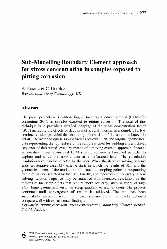
This section shows the results of the sub-modelling technique in a test sample. The initial topography of the sample has been recorded with a grid spacing of 6.345 µm. Figure 5 shows the results of the SCF in two different sub-models, one containing the other. The space resolution in the larger sub-model is 50.76µm by 50.76 µm, the space resolution for the most inner sub-model is 6.345 µm by 6.345 µm. In this case, the small sub-model has captured a small pit responsible for a SCF of nearly 2.



Figure 3: Normalised Y-Y component of the stress tensor for sub-models of different depths.

Figure 4: Sequence of sub-models with different depths used to determine a rule for defining the optimum size, for thick plates exposed to pitting corrosion. The greyscale in the top surface indicates Syy.



Figure 5: Pit detected during the sub-modelling iterations. The square window represents the region of high resolution covered by a submodel when scanning the whole sample.

Figure 6 shows some preliminary results obtained for a sample of 33 43 3.175mm mm mm× × , in which many pits of different scales (typically 20 µm) are randomly distributed. The greyscale in the figure indicates SCF while the circles spot regions with peaks of SCF that significantly exceed the local average. Cracks are more likely to originate in these regions. The results obtained in this figure are in good agreement with experimental findings during fatigue tests.

5 Conclusions

A Sub-Modelling - Boundary Element approach for computing SCFs in samples exposed to pitting corrosion has been developed, and practical rules for defining the sub-model elaborated.



Figure 6.

The research behind this presentation is still being undertaken. The goal of representing a SCF mapping of a sampled surface to the most available level of accuracy has been achieved. The tool has been successfully tested in several real case scenarios, and the results obtained compare well with experimental findings.

Acknowledgements

The authors of this work would like to acknowledge the support provided by Dr John Baynham and Dr Robert Adey, and the use of BEASY MECHANICAL DESIGN software.

References

[1] Kolotyrkin, Ya. M. Pitting corrosion of metals. Corrosion 19: 261t, 1963.



[2] Szklarska-Smialowska, Z. Localized Corrosion, Staehle, Brown, Kruger and Agrawal, eds., p. 312. National Assoc. of Corros. Engrs., Houston, 1974.

[3] Kruger, J. in Passivity and Its Breakdown on Iron and Iron Base Alloys, Staehle and Okada, eds., p. 91. Nat. Assoc. of Corros. Engrs., 1976.

[4] S. M. Sharland. A review of the theoretical modelling of crevice and pitting corrosion. Corrosion Science. 27 (3), pp 289-323, 1987.

[5] A. P. Jivkov. Evolution of fatigue crack corrosion from surface irregularities. Theoretical and Applied Fracture Mechanics. 40, pp 45-54, 2003.

[6] S. I. Rokhlin, J.-Y. Kim, H. Nagy, B. Zoofan. Effect of pitting corrosion on fatigue crack initiation and fatigue life. Engineering Fracture Mechanics 62 pp. 425-444, 1999.

[7] R. E. Melchers and R. J. Jeffrey, Probabilistic models for steel corrosion loss and pitting of marine infrastructure, Reliability Engineering and System Safety (2007), doi:10.1016/j.ress.2006.12.006.

[8] Beasy Mechanical Design software. www.beasy.com [9] C. A. Brebbia, J. C. F. Telles, and L. C. Wrobel. Boundary Element

Techniques. Theory and Applications in Engineering. Springer-Verlag, Berlin, Heidelberg, NY, Tokyo, 1984

[10] GID resources. Commercial pre and post-processor software. url: http://gid.cimne.upc.es



Documents

Sub-Modelling Boundary Element approach for stress concentration · PDF fileSub-Modelling Boundary Element approach for stress concentration in samples exposed to pitting corrosion