NeuroImage 176 (2018) 454–464

Contents lists available at ScienceDirect

NeuroImage

journal homepage: www.elsevier.com/locate/neuroimage

Sub-millimeter ECoG pitch in human enables higher fidelity cognitiveneural state estimation

John Hermiz a, Nicholas Rogers b, Erik Kaestner c, Mehran Ganji a, Daniel R. Cleary d,Bob S. Carter d, David Barba d, Shadi A. Dayeh e,f, Eric Halgren g,h, Vikash Gilja a,*

a Department of Electrical and Computer Engineering, University of California San Diego, La Jolla, CA 92093, USAb Department of Physics, University of California San Diego, La Jolla, CA, 92161, USAc Neurosciences Program, University of California San Diego, La Jolla, CA, 92096, USAd Department of Neurosurgery, University of California San Diego, La Jolla, CA, 92103, USAe Department of Nanoengineering, University of California San Diego, La Jolla, CA, 92093, USAf Department of Materials Science and Engineering, University of California San Diego, La Jolla, CA, 92093, USAg Department of Radiology, University of California San Diego, La Jolla, CA, 92103, USAh Department of Neurosciences, University of California San Diego, La Jolla, CA, 92103, USA

A R T I C L E I N F O

Keywords:microECoGHumanMachine-learningPEDOTElectrodeLanguage

Abbreviation: HFB, high frequency band; ACC, creference; MVN, Multivariate normal.* Corresponding author.E-mail address: vgilja@ucsd.edu (V. Gilja).

https://doi.org/10.1016/j.neuroimage.2018.04.027Received 2 November 2017; Received in revised foAvailable online 18 April 20181053-8119/© 2018 Published by Elsevier Inc.

A B S T R A C T

Electrocorticography (ECoG), electrophysiological recording from the pial surface of the brain, is a criticalmeasurement technique for clinical neurophysiology, basic neurophysiology studies, and demonstrates greatpromise for the development of neural prosthetic devices for assistive applications and the treatment of neuro-logical disorders. Recent advances in device engineering are poised to enable orders of magnitude increase in theresolution of ECoG without comprised measurement quality. This enhancement in cortical sensing enables theobservation of neural dynamics from the cortical surface at the micrometer scale. While these technical capa-bilities may be enabling, the extent to which finer spatial scale recording enhances functionally relevant neuralstate inference is unclear.

We examine this question by employing a high-density and low impedance 400 μm pitch microECoG (μECoG)grid to record neural activity from the human cortical surface during cognitive tasks. By applying machinelearning techniques to classify task conditions from the envelope of high-frequency band (70–170Hz) neuralactivity collected from two study participants, we demonstrate that higher density grids can lead to more accuratebinary task condition classification. When controlling for grid area and selecting task informative sub-regions ofthe complete grid, we observed a consistent increase in mean classification accuracy with higher grid density; inparticular, 400 μm pitch grids outperforming spatially sub-sampled lower density grids up to 23%. We alsointroduce a modeling framework to provide intuition for how spatial properties of measurements affect theperformance gap between high and low density grids. To our knowledge, this work is the first quantitativedemonstration of human sub-millimeter pitch cortical surface recording yielding higher-fidelity state estimationrelative to devices at the millimeter-scale, motivating the development and testing of μECoG for basic and clinicalneurophysiology as well as towards the realization of high-performance neural prostheses.

Introduction

Recent advances in device engineering and human neurophysiologyhas stimulated interest in recording electrical activity from the surface ofthe brain, a technique referred to as Electrocorticography (ECoG).

lassification accuracy; ELR, elast

rm 9 March 2018; Accepted 11 A

Current studies have demonstrated that ECoG probe features can beshrunk to sub-mm scales (μECoG) with devices that have remarkablesubstrate flexibility allowing the probes to conform to the surface of thebrain (Castagnola et al., 2015; Ganji et al., 2017; Insanally et al., 2016;Kellis et al., 2009; Khodagholy et al., 2016, 2014; 2011; Toda et al., 2011;

ic-net logistic regression; STG, superior temporal gyrus; CAR, common average

pril 2018

J. Hermiz et al. NeuroImage 176 (2018) 454–464

Trumpis et al., 2017). Novel devices also demonstrate the integration offlexible electronics on these substrates, which could result in a newgeneration of ultra-high density probes with 1,000s to 10,000s of elec-trodes (Fang et al., 2017; Viventi et al., 2011). New methods for applyingorganic materials, in particular poly(3,4-ethylenedioxythiophene) dopedwith polystyrene sulfonate (PEDOT:PSS), have yielded relatively lowimpedance (Ganji et al., 2017; Khodagholy et al., 2014, 2011) electrodeswith areas as small as 10 μm2 (Khodagholy et al., 2016), enabling elec-trophysiology with high signal fidelity. These proof of concept technol-ogies have enabled neurophysiologists to discover novel neural dynamicsfrom the surface of the brain, including recurrent spiral waves manifestedfrom seizures in animal model (Viventi et al., 2011) and single unit ac-tivity in both animal model and studies in the clinic (Khodagholy et al.,2016, 2014). These developments could lead to advances in basicneuroscience research and medical applications such as clinical mappingand brain-machine interfaces (Blakely et al., 2008; Bleichner et al., 2016;Branco et al., 2016; Chang, 2015; Ganji et al., 2017; Hwang andAndersen, 2013; Jiang et al., 2017; Kaiju et al., 2017; Kellis et al., 2010;Leuthardt et al., 2009; Maharbiz et al., 2017; Muller et al., 2016b).

A major question raised in the advancement of device technology is,“How dense should surface grids be?” There is likely no universalanswer to this question, since relevant parameters are applicationdependent and, in particular, the spatial characteristics of neural ac-tivity could vary between cortical regions and functional settings.Previous simulation and empirical studies have used spatial spectraltechniques to estimate the ideal spacing to be 1.25 mm (Freeman et al.,2000; Slutzky et al., 2010). Other empirical works have quantifiedspatial characteristics by using similarity metrics such as channel cor-relation vs channel distance (Chang, 2015; Insanally et al., 2016; Kelliset al., 2016; Muller et al., 2016b; Trumpis et al., 2017) with the inter-pretation that steeper falloffs indicate that high density grids are ad-vantageous. However, a well-defined functional interpretation of thesefalloff curves has not been established. In this work, we develop anillustrative model to gain an intuition for how spatial signal and noiseproperties affect the performance gap between high and low densitygrids from a machine learning perspective. Furthermore, we apply thisperspective to examine sub-millimeter pitch grid recordings from thehuman cortical surface.

Typical adult clinical ECoG probes have an interelectrode spacings(“pitch”) of 1 cm, and research grids with pitches as low as 30 μm havebeen used intraoperatively (i.e. Neurogrid) (Chang, 2015; Khodagholyet al., 2016, 2014). Previous electrophysiology studies demonstrated thatgrids with pitches below 1 cm capture richer electrophysiology, and anumber of research studies employ “HD-ECoG” grids with 3–4mm pitchthat are manufactured by the same companies with the same processes and

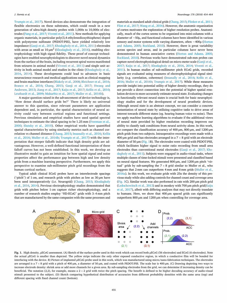
Fig. 1. High density, μECoG assessment. (A) Sketch of the surface probe used in this wthe actual μECoG is smaller than depicted. The yellow strips indicate the only othinterfacing with the device. B) Picture of implanted μECoG probe used in this work, ware arranged is a 7� 8 grid with a pitch of 400 μm, a diameter of 50 μm, and coatedincrease electrode density: shrink area or add more channels for a given area. By sub-beneficial. The notation (2,2), for example, means a 2� 2 grid with twice the pitchstimuli presented to the subject. (D) Sketch comparing hypothetical distribution odifferent spacing with fixed channel count (bottom).

455

materials as standard adult clinical grids (Chang, 2015; Flinker et al., 2011;Flint et al., 2017; Wang et al., 2016). However, the anatomic organizationof cortex motivates the exploration of higher resolution probes. Anatomi-cally, much of the cortex seems to be organized into mini-columns with adiameter of ~50μ, and functional columns have been identified in varioussensory and motor systems with varying diameters, often ~400μ (Hortonand Adams, 2005; Rockland, 2010). However, there is great variabilityacross species and areas, and in particular columns have never beendemonstrated in human associative cortex (Horton and Adams, 2005;Rockland, 2010). Previous works have demonstrated sub-mm probes cancapture novel electrophysiological detail onmicro-meter scale (Ganji et al.,2017; Kaiju et al., 2017; Khodagholy et al., 2016, 2014; Viventi et al.,2011). In human studies of sub-millimeter pitch ECoG grids, recordedsignals are evaluated using measures of electrophysiological signal simi-larity (e.g. correlation, coherence) (Insanally et al., 2016; Kellis et al.,2016; Muller et al., 2016b; Trumpis et al., 2017). While these measuresprovide insight into potential utility of higher density recordings, they donot provide a direct connection into the potential of higher spatial reso-lution devices tomore accurately estimate neural state. Evaluating changesin functionally relevant neural states is crucial both for basic neurophysi-ology studies and for the development of neural prosthetic devices.Although neural state is an abstract concept, we can consider a concreteinstantiation of neural state by utilizing cognitive tasks to drive areas ofinterest towards different states (eg. hearing human voice vs noise). Thenwe apply machine learning algorithms to evaluate if the additional viewsof neural state provided by higher resolution recording improves ourability to classify task conditions from neural activity alone. In this work,we compare the classification accuracy of 400 μm, 800 μm, and 1200 μmpitch grids from two subjects. Intraoperative recordings were made with a400 μm grid and has electrodes arranged in a 7� 8 grid with an electrodediameter of 50 μm (Fig. 1B). The electrodes were coated with PEDOT:PSS,which facilitates higher signal to noise ratio recording from small areaelectrodes than conventional metal electrodes (Ganji et al., 2017; Kho-dagholy et al., 2011). Subjects were engaged in audio-visual tasks, wheremultiple classes of time-locked stimuli were presented and classified basedon neural signal features. We generated 800 μm, and 1200 μm pitch “vir-tual” grids by sub-sampling the 7� 8 grid similar to Muller et al., whosuggests that 2mm can outperform 4mm and 8mm grids (Muller et al.,2016a). In this work, we evaluate grids with 25x the density of this pre-vious study while also adding controls for channel count and coverage area(Fig. 1C). Similar work was also performed in rats with 200 μm pitch grid(Ledochowitsch et al., 2013) and in monkey with 700 μm pitch grid(Kaijuet al., 2017), albeit with differing analyses that may not directly translateto humans. Here, we show that 400 μm spaced grids can significantlyoutperform 800 μm and 1200 μm when controlling for coverage area.

ork which can record both μECoG (56 electrodes) and ECoG (6 electrodes). Noteer exposed conductive region, in which a conductive film will be bonded forhich was manufactured using micro/nano-fabrication techniques. The electrodeswith PEDOT:PSS. The scale bar is 400 μm. (C) Drawing depicting two ways to

sampling electrodes from the grid, we can determine if increasing density can bespacing. The benefit is defined to be higher decoding accuracy of audio-visualf accuracies from different probability densities with the same area (top) and

Table 1Commonly used symbols.

Symbol Description Symbol Description

σs characteristic length forsignal

s signal across channels

λ characteristic length fornoise

Σ channel co-variance matrix

a signal amplitude for centerchannel

d 2m squared Mahalanobis

distancex measurements across

channelsΔ difference in squared Mahal.

distance

J. Hermiz et al. NeuroImage 176 (2018) 454–464

Methods

Please refer to Table 1 for commonly used symbols used throughoutthe text.

Modeling

DescriptionTo explore when higher density grids might outperform (or under-

perform) comparable lower density grids, a model was developed andstudied under various circumstances. Let x be a d-dimensional mea-surement or feature vector of real numbers, where d is the channel count.In general, x is assumed to include signal and additive noise.

x ¼ sþ n (1)

Two conditional random variables are defined xp ¼ x��c ¼ p and

xnp ¼ x��c ¼ np, where c denotes the class a particular feature vector be-

longs to: p (preferred stimuli) or np (non-preferred stimuli). We will as-sume only the preferred stimuli has signal. Previous studies have shownthat correlation between raw channels measurements and featuresderived from various frequency bands can fit reasonably well to anexponential decay (Insanally et al., 2016; Kellis et al., 2016; Muller et al.,2016b; Trumpis et al., 2017). This motivated defining the signal to decayexponentially with respect to Euclidean distance from the peak activationsite.

si ¼ a*exp�� jjri � rctrjj

σs

�(2)

Note, ri is the position of the ith channel and rctr is the position of thechannel with peak (or center) activation. a scales the magnitude of signaland, as will subsequently become evident, is the signal to noise ratio(SNR) for the center channel. σs is the characteristic length for the signal,which is when jjri � rctr jj ¼ σs corresponding to a 1/e� 0.37 decrease inthe signal. For simplicity, the noise is assumed to be Gaussian with zeromean and unit variance ðΣii ¼ 1Þ, n � Nð0;ΣÞ; hence, SNR, which isdefined to be the mean divided by the standard deviation for the centerchannel is a. Again, it is assumed that noise covariance decays expo-nentially as a function of distance. Here, λ is the characteristic length ofnoise correlation. So, two electrodes that are spaced λ units apart fromeach other will have a correlation of 1/e� 0.37.

Σij ¼ exp������ri � rj

����λ

�(3)

The overall model can be rewritten as

xp � Nðs;ΣÞ (4)

xnp � Nð0;ΣÞ (5)

AnalysisThis simple, yet plausible model allows us to explore situations in

456

which higher density grids outperform lower density grids. We aremainly interested in two comparisons: 1) fix area and vary channel count(or equivalently pitch) and 2) fix channel count and vary pitch (orequivalently area). In order to compare grids, we need a metric. Since xp

and xnp are drawn from multivariate normal distributions with the samecovariance matrix, the natural choice is the Mahalanobis distance, dmbetween the means of the distributions.

d2m ¼ sTΣ�1s (6)

In fact, researchers in related work have used the Mahalanobis dis-tance to score “evoked signal-to-noise ratio” in trials indicating that theseassumptions are reasonable (Insanally et al., 2016; Trumpis et al., 2017).

Intuitively, dm is the average separation between feature vectors from thepreferred and non-preferred stimuli. The larger the separation, the morediscriminable the two classes of data are. What we are interested in ishow that separation changes as a function of grid density. That is, thedifference or difference squared,

Δ ¼ d2m;hd � d2m;ld (7)

To gain an intuition for when higher density grids have an advantage,we compute analytical expressions for Δ in the two-channel case: 1) thedifference between two vs one channel, Δ2,1 and 2) the difference be-tween two channels that are 1 unit apart vs 2 units apart, Δ2,2’.

Δ2;1 ¼ ðs2 � s1Σ21Þ21� Σ2

21

(8)

Δ2;2' ¼ðs2 � s1Σ21Þ2�

1� Σ221

� � ðs2' � s1Σ2'1Þ2�1� Σ2

2'1

� (9)

See Sections A4.1-A4.2 for derivation. As is obvious from Eqns (8) and(9), there is a singularity when Σ21 ¼ 1 or Σ2'1 ¼ 1. This occurs becausethe squared Mahalanobis distance, d2x1 ;x2 or d

2x1 ;x'2

cannot be computed as

detðΣÞ becomes undefined and Σ uninvertible. This likely never occurs inpractice as there is always measurement noise that is not perfectlycorrelated across channels.

Time seriesA simple time series extension of the spatial model is described. The

measurement vector, x that has d elements for the number of channelsbecomes a matrix, X that is d x T, where T is number of time samples.Again, we will assume in general that the signal is deterministic and thatthere is additive noise.

X ¼ SþN (10)

In the non-preferred condition, S ¼ 0 and in the preferred condition S ¼F where F are samples for a set of deterministic functions that evolve overspace and time. The rows of F are denoted f 1; f 2; :: f d. As before, thesignal on each channel decays exponentially with distance from thecenter channel, xctr which we will set to be x1.

f j ¼ f 1 exp������r1 � rj

����σs

�(11)

The time evolution of f 1 is assumed to follow a Gaussian shape wherethe peak activation occurs at tpk.

f 1 ¼ a exp������t � tpk

����σt

�(12)

Finally, the noise matrix N are just T copies of the original model'srandom variable n, so that it’s entries across time are independent andidentically distributed. Hence, the noise spatial relationship of Eqn (3)still holds.

J. Hermiz et al. NeuroImage 176 (2018) 454–464

Probe

The probe used in experiments consists of 56 μECoG and 6 ECoGelectrodes. The μECoG electrodes are arranged in a 7� 8 grid with a400 μmpitch and an electrode diameter of 50 μm. The ECoG electrodes arearranged is a strip or line spaced 1 cm apart with an electrode diameter of3mm. The μECoG were used to record surface potentials while the most ofthe ECoG electrodes were tied to reference. A stainless steel needle probewas used for ground and was inserted into the scalp at the edge of thecraniotomy. The electrodes are coatedwith an organic conducting polymercalled poly(3,4-ethylenedioxythiophene) doped with polystyrene sulfo-nate (PEDOT:PSS). PEDOT:PSS has been shown to reduce impedancevalues by orders of magnitude compared to traditional metal electrodes(eg. Pt). The typical electrode impedance magnitude at 1 kHz is 13 kΩ.Lastly, the substrate is 4–5 μm thick parylene which can conform to thesurface of the brain. Additional device details can be found in (Ganji et al.,2017; Uguz et al., 2016). The data acquisition system used is describedextensively in (Hermiz et al., 2016) and briefly in Section A.1.

Sub-sampling

The 7� 8 grid of electrodes was sub-sampled to obtain “virtual” grids.There are many ways to sub-sample and an exhaustive enumeration of allpossible sub-samples is not only intractable, but would be challenging tointerpret. Since we are interested in determining if certain grid densitiesare beneficial we chose to limit all virtual grids to be square as thesevirtual grids could easily be parameterized and related to electrodedensity.

Virtual square grids can be parameterized by 3 variables (ignoringelectrode size): number of channels, pitch (or spacing), and the area thatthe grid encompasses. If pitch is normalized to take on integer values (1,2, …), then we can relate the variables using the following expression:A ¼ ðpð ffiffiffi

cp � 1Þ2, where A, p and c are the area, pitch and number of

channels, respectively. We explored the device parameter space by fixingeach variable for a given analysis and changing the other degree offreedom: fixed pitch (Fig. 6), fixed area (Fig. 7), and fixed channel count(Fig. S7). We are primarily interested in comparing virtual devices withfixed area (Fig. 7).

Since our grid contained bad recording channels, we only consideredvirtual grids that had at least 50% of the channels they were supposed tohave. For example, let's say a 5� 5 grid had 13 good recording channels(52%), then the virtual grid would not be thrown out; however, it had 12good recording channels (48%), then the virtual grid would be thrownout.

In some situations, it might be the case that a grid with 50% goodelectrodes is compared to a grid with 90% good electrodes, in which casethe percentage of good channels confounds the comparison. To ensurethere our results were not biased by the confounding variable of per-centage of good channels, we performed a meta-analysis where we foundthe difference in percentage of good channels for all comparisons anddetermined if the distributions were significantly biased away from 0.Wedid not find a significant bias for the fixed area comparison, but did find abias for the fixed channel comparison for SD007 (Fig. S8). We discuss theinterpretation of the fixed channel comparison results in light of this biasin the Discussion and Section A.9.

Machine learning

Features were computed by summing up the HFB for each channel innon-overlapping windows of 0.25 s. For SD007, the start and end timewere 0.15 and 0.9 s post stimulus onset and for SD008, the start and endtime were 0.5–1 s post stimulus. Elastic-net logistic regression (ELR) wasused to classify presented stimuli types. ELR was used because it is robustto high dimensional datasets and generally yields competitive classifi-cation accuracies (Zou and Hastie, 2005). ELR is a regularized version of

457

logistic regression. It uses a combination of ridge (L2-penalty) and lasso(L1-penalty) regularization to reduce and eliminate the effect ofnon-discriminatory features. Ultimately, the result in a linear discrimi-nate that should have few, high magnitude weights. The ELR imple-mentation used was Glmnet Toolbox for Matlab (Qian et al., 2013). Themix of L1 and L2 penalty was fixed to be 0.75 and 0.25, while the weightof the regularization penalty was chosen by sweeping through 50candidate values 12 times (for 12-fold cross validation) and choosing thevalue that maximizes the average accuracy. Aggregate accuracy statisticsare computed from validation sets.

Experimental task

Subjects SD007 and SD008 undergoing clinical mapping of eloquentcortex provided informed consent to have the probe placed on their pialsurface and to participate in a 10-min task. The μECoG grid was placed onthe left superior temporal gyrus (STG): anterior STG for SD007 andposterior STG for SD008. UC San Diego Health Institutional ReviewBoard (IRB) reviewed and approved study protocol.

The preferred and non-preferred categories were assigned by visuallyinspecting the trial averages of the high frequency band envelope. Thecategory that yielded the largest response was labeled preferred while thecategory that yielded the smallest or no response was labeled non-preferred.

SD007 read visual words (e.g text of the word ‘lion’), repeatedauditory words (eg. audio of the word ‘lion’), and named visual pictures(eg. picture of a ‘lion’). The stimuli that elicited the largest response wasthe auditory word, therefore it was labeled preferred. Both visual picturesand words yielded little if any response. Visual words were chosen to bein the analysis and were labeled non-preferred. It is expected that theauditory word elicits the largest response since the probe was implantedon STG, which is responsible for auditory processing. There were 60auditory word trials and 59 visual word trials analyzed in this study.

SD008 saw a 3-letter string (GUH, SEE) and then heard an auditory 2-phoneme combination, making a decision whether the visual and audi-tory stimuli matched. Interspersed were visual control trials in which afalse font was followed by a real auditory stimulus and auditory controltrials in which a real letter string was followed by a 6-band noise-vocoded2-phoneme combination. For SD008, binary classification was performedbetween noise-vocoded stimuli and human voice. In these recordings, thenoise-vocoded stimuli produce a larger response than human voice andtherefore the noise-vocoded was labeled preferred while human voicewas labeled non-preferred. This is consistent with previous work exam-ining cognitive processing and evoked responses to noise-vocoded andhuman voice in posterior STG (Travis et al., 2013). There were 68noise-vocoded trials and 63 human voice trials analyzed in this study.

Results

Modeling and experimental analyses were performed to determine ifand when higher density grids outperform lower density grids. Anillustrative model with properties motivated from previous studies(Insanally et al., 2016; Kellis et al., 2016; Muller et al., 2016b; Trumpiset al., 2017) was developed to determine under what conditions a higherdensity grid might outperform a lower density grid. Analytical results forthe simple 2-channel case and numerical results for higher dimensionalcases are presented (Fig. 2). We then analyze real μECoG recordings ac-quired from two subjects, SD007 and SD008 engaged in audio-visualtasks in the operating room. Two types of stimuli were classified andclassification accuracy served as the performance metric whencomparing grids. Sub-sampling the 7� 8 grid allowed us to explore thedevice design space and, in particular, electrode density.

Modeling

We developed a simple model that assumes measurements belong two

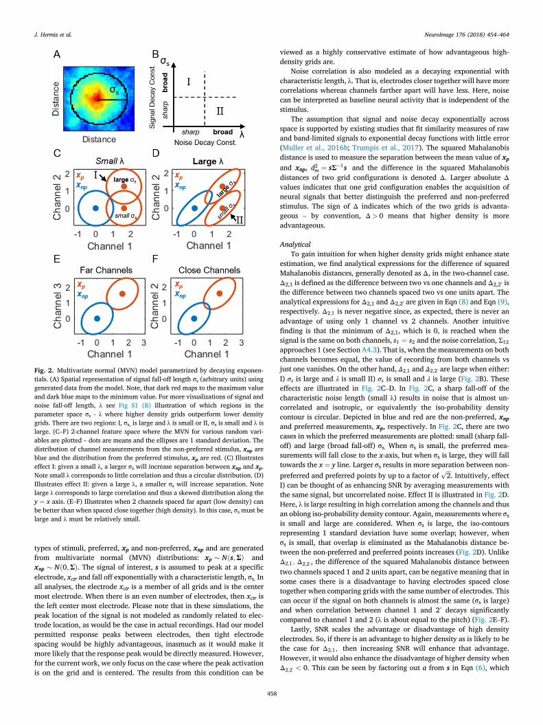
Fig. 2. Multivariate normal (MVN) model parametrized by decaying exponen-tials. (A) Spatial representation of signal fall-off length σs (arbitrary units) usinggenerated data from the model. Note, that dark red maps to the maximum valueand dark blue maps to the minimum value. For more visualizations of signal andnoise fall-off length, λ see Fig S1 (B) Illustration of which regions in theparameter space σs - λ where higher density grids outperform lower densitygrids. There are two regions: I, σs, is large and λ is small or II, σs is small and λ islarge. (C–F) 2-channel feature space where the MVN for various random vari-ables are plotted – dots are means and the ellipses are 1 standard deviation. Thedistribution of channel measurements from the non-preferred stimulus, xnp areblue and the distribution from the preferred stimulus, xp are red. (C) Illustrateseffect I: given a small λ, a larger σs will increase separation between xnp and xp.Note small λ corresponds to little correlation and thus a circular distribution. (D)Illustrates effect II: given a large λ, a smaller σs will increase separation. Notelarge λ corresponds to large correlation and thus a skewed distribution along they ¼ x axis. (E–F) Illustrates when 2 channels spaced far apart (low density) canbe better than when spaced close together (high density). In this case, σs must belarge and λ must be relatively small.

J. Hermiz et al. NeuroImage 176 (2018) 454–464

types of stimuli, preferred, xp and non-preferred, xnp and are generatedfrom multivariate normal (MVN) distributions: xp � Nðs;ΣÞ andxnp � Nð0;ΣÞ. The signal of interest, s is assumed to peak at a specificelectrode, xctr and fall off exponentially with a characteristic length, σs. Inall analyses, the electrode xctr is a member of all grids and is the centermost electrode. When there is an even number of electrodes, then xctr isthe left center most electrode. Please note that in these simulations, thepeak location of the signal is not modeled as randomly related to elec-trode location, as would be the case in actual recordings. Had our modelpermitted response peaks between electrodes, then tight electrodespacing would be highly advantageous, inasmuch as it would make itmore likely that the response peak would be directly measured. However,for the current work, we only focus on the case where the peak activationis on the grid and is centered. The results from this condition can be

458

viewed as a highly conservative estimate of how advantageous high-density grids are.

Noise correlation is also modeled as a decaying exponential withcharacteristic length, λ. That is, electrodes closer together will have morecorrelations whereas channels farther apart will have less. Here, noisecan be interpreted as baseline neural activity that is independent of thestimulus.

The assumption that signal and noise decay exponentially acrossspace is supported by existing studies that fit similarity measures of rawand band-limited signals to exponential decay functions with little error(Muller et al., 2016b; Trumpis et al., 2017). The squared Mahalanobisdistance is used to measure the separation between the mean value of xpand xnp, d2m ¼ sΣ�1s and the difference in the squared Mahalanobisdistances of two grid configurations is denoted Δ. Larger absolute Δvalues indicates that one grid configuration enables the acquisition ofneural signals that better distinguish the preferred and non-preferredstimulus. The sign of Δ indicates which of the two grids is advanta-geous – by convention, Δ> 0 means that higher density is moreadvantageous.

AnalyticalTo gain intuition for when higher density grids might enhance state

estimation, we find analytical expressions for the difference of squaredMahalanobis distances, generally denoted as Δ, in the two-channel case.Δ2,1 is defined as the difference between two vs one channels and Δ2,20 isthe difference between two channels spaced two vs one units apart. Theanalytical expressions for Δ2,1 and Δ2,20 are given in Eqn (8) and Eqn (9),respectively. Δ2;1 is never negative since, as expected, there is never anadvantage of using only 1 channel vs 2 channels. Another intuitivefinding is that the minimum of Δ2,1, which is 0, is reached when thesignal is the same on both channels, s1 ¼ s2 and the noise correlation, Σ12

approaches 1 (see Section A4.3). That is, when themeasurements on bothchannels becomes equal, the value of recording from both channels vsjust one vanishes. On the other hand, Δ2;1 and Δ2;2' are large when either:I) σs is large and λ is small II) σs is small and λ is large (Fig. 2B). Theseeffects are illustrated in Fig. 2C–D. In Fig. 2C, a sharp fall-off of thecharacteristic noise length (small λ) results in noise that is almost un-correlated and isotropic, or equivalently the iso-probability densitycontour is circular. Depicted in blue and red are the non-preferred, xnpand preferred measurements, xp, respectively. In Fig. 2C, there are twocases in which the preferred measurements are plotted: small (sharp fall-off) and large (broad fall-off) σs. When σs is small, the preferred mea-surements will fall close to the x-axis, but when σs is large, they will falltowards the x ¼ y line. Larger σs results in more separation between non-preferred and preferred points by up to a factor of

ffiffiffi2

p. Intuitively, effect

I) can be thought of as enhancing SNR by averaging measurements withthe same signal, but uncorrelated noise. Effect II is illustrated in Fig. 2D.Here, λ is large resulting in high correlation among the channels and thusan oblong iso-probability density contour. Again, measurements where σsis small and large are considered. When σs is large, the iso-contoursrepresenting 1 standard deviation have some overlap; however, whenσs is small, that overlap is eliminated as the Mahalanobis distance be-tween the non-preferred and preferred points increases (Fig. 2D). UnlikeΔ2;1; Δ2;2' , the difference of the squared Mahalanobis distance betweentwo channels spaced 1 and 2 units apart, can be negative meaning that insome cases there is a disadvantage to having electrodes spaced closetogether when comparing grids with the same number of electrodes. Thiscan occur if the signal on both channels is almost the same (σs is large)and when correlation between channel 1 and 2’ decays significantlycompared to channel 1 and 2 (λ is about equal to the pitch) (Fig. 2E–F).

Lastly, SNR scales the advantage or disadvantage of high densityelectrodes. So, if there is an advantage to higher density as is likely to bethe case for Δ2;1; then increasing SNR will enhance that advantage.However, it would also enhance the disadvantage of higher density whenΔ2;2' < 0. This can be seen by factoring out a from s in Eqn (6), which

Fig. 3. (A–D) Numerical results from (5,1) vs (3,2) and (3,1) vs (3,2). The no-tation (a,b) refers to a grid that has a by a channels and has a pitch of b. (A–B) AsSNR increases, the difference of squared Mahalanobis distance (Δd2m) increasesor decreases, depending on σs, λ and which grids are compared. (C–D) 3d plotsshowing Δd2m for a grid of σs and λ values. (C) For (5,1) – (3,2), there are novalues for which Δd2m< 0, given the domain; and as expected, Δd2m » 0, whenσs, is large and λ is small or vice versa. (D) For (3,1) - (3,2), Δd2m< 0, whenroughly, σs> 5 and 1< λ< 2, which is expected. Again, Δd2m » 0 when σs, islarge and λ is small or vice versa. The color axis ranges from �1 (dark blue) to 1(dark red) and is used to represent sign.

J. Hermiz et al. NeuroImage 176 (2018) 454–464

shows that d2m∝a2 and thus Δ∝a2. This SNR scaling effect is true for thegeneral d-channel case.

NumericalTo determine whether the effects found in the analytical expressions

of the 2-channel case generalized to higher dimensional cases, the 25-channel results were numerically computed from Eqn (6). Again, twocomparisons were made: 1) fixed area, comparing a 5� 5 grid with unitpitch vs a 3� 3 grid with twice unit pitch and 2) fixed channel count,comparing a 3� 3 grid with unit pitch vs a 3� 3 grid with twice unitpitch. The difference in squared Mahalanobis distances for 1) and 2) willbe denoted as Δ5;3' and Δ3;3' , respectively.

As expected, SNR scales the difference in performance Δ5;3' and Δ3;3' :

In Fig. 3A, both Δ5;3' and Δ3;3' > 0 for σs ¼ 0:5 and λ ¼ 1, so increasingSNR increases the difference in squared Mahalanobis distance quadrati-cally. Interestingly, Fig. 3B shows for σs ¼ 10 and λ ¼ 1 high densityprovides an advantage or disadvantage depending the comparison:Δ5;3' > 0 and Δ3;3' < 0: Hence, SNR quadratically increases Δ5;3' anddecreases Δ3;3' . These results follow directly from our analytical findingsdescribed in the last paragraph of Section 3.1.1.

Consistent with the effects found in the analytical expressions of the2-channel case, there are two regions in σs-λ space where higher densityoutperforms: I) σs < 1 and λ > 1 or II) σs > 1 and λ < 1 for Δ5;3' and λ <

1=3 for Δ3;3' (Fig. 3C–D). As anticipated from our 2-channel analyticalresults, there is a region where higher density underperforms whencomparing grids with the same channel count, which is roughly σs ≫ 1and 1=2 < λ < 2. Finally, as expected, Δ5;3' > 0 for all computed valuesin the domain 0:1 � σs; λ � 10, or, simply put, the 3� 3 grid with twiceunit spacing never outperforms the 5� 5 grid with 1 unit spacing for allthe parameters we used.

Time seriesIt is important to note that the presented model has no notion of time,

but simple extensions can be made to model time. One extension is tohave the signal evolve according to a Gaussian function and assume thenoise is independent and identically distributed across time (see Section2.1.3 for explicit definition). An important statistic often computed fromhigh density recordings is the correlation between two channels vs thedistance between those channels. The correlation between the centerchannel, x1 and any other channel xj is (see Section A4.4 for derivation)

ρx1xj ¼�Σ1j þ αjp� μ1μj

�ffiffiffiffiffiffiffiffiffiffiffiffiffiffiffiffiffiffiffiffiffiffiffiffiffiΣ11 þ p� μ21

p ffiffiffiffiffiffiffiffiffiffiffiffiffiffiffiffiffiffiffiffiffiffiffiffiffiffiffiffiΣjj þ α2

j p� μ2jq 13

where αj ¼ exp�

�jjr1�rjjjσs

�, Σ1j ¼ exp

�� jjr1�rjjj

λ

�, p ¼ E½f 21�, μ1 ¼ E½x1�

and E½xj� ¼ μj. Numerical calculations suggested out that ρx1xj � Σ1j

when SNR in x1 is not too large (Fig. S2). That is, if the SNR is not toolarge, then the channel correlation computed from the time series of thismodel, will be approximately equal to the entries of the noise covariancematrix. Under these circumstances, we can extend the results of thespatial model to this time series model. This is important because we caninterpret commonly computed correlation vs distance plots using ourframework.

Empirical

Next, we explore the advantages of higher density grids by analyzingreal μECoG recordings from two subjects intraoperatively at UC SanDiego, Thornton Hospital. The grid has 7� 8 micro-electrodes spaced400 μm apart and a diameter of 50 μm. These subjects were engaged in anaudio-visual task (see Section 2.5). Various types of time locked stimuliwere presented to the subjects and stimuli class served as ground truth foroffline neural state decoding experiments. For each subject, there were 2

459

stimulus classes classified: one that produced a marked neural responseand one that did not. Rectified high frequency band (70–170Hz)amplitude (HFB) was used to measure the neural response because it hasbeen shown to have high spatial specificity and correlation with sensoryand cognitive processing (Crone et al., 1998; Miller et al., 2007).Fig. 4A–C shows how the raw trials were processed to yield HFB (SectionA.2). The trials were then parsed into 0.25 s windows and summed tocompute the features (Section 2.4).

The spatial spread of HFB activation was qualitatively assessed bytaking the peak HFB in time and using cubic interpolation across space(Fig. 4D–G). The plots for each subject are normalized to indicated thepercentage of the peak response. For both subjects, there is a clear regionwhere the activation is markedly larger. For SD007, the highly-activatedregion appears to be confined to a smaller area and the dynamic range islarger than SD008. The preferred and non-preferred stimuli were

Fig. 4. Signal processing pipeline. (A) Trials of raw measurements (no post processing) shown in gray and the trial average is shown as black (B) Block diagram ofsignal processing (C) Trials of high frequency band (HFB) activity shown in gray and the trial average is shown as black. Cubic interpolation across space of peak HFBdue to preferred stimuli (D) SD007 and (E) SD008 vs non-preferred stimuli (F) SD007 and (G) SD008. Units are percent of maximum response across stimuli type foreach subject. White space could not be interpolated due to lack of channels. Single channel ACC for (H) SD007 and (I) SD008. White squares indicate thrownout channels.

J. Hermiz et al. NeuroImage 176 (2018) 454–464

classified by applying the HFB features to Elastic Net Logistic Regression(ELR) – a classification algorithm robust to high dimensional datasetswith a limited number of examples (Qian et al., 2013; Zou and Hastie,2005) (Section 2.4). The single channel classification accuracy (ACC)results are consistent with the heatmaps of the HFB activation(Fig. 4H–I). Maximum single channel ACC for SD007 and SD008 is 78%and 77%, respectively. Note, chance performance is 50% since classifi-cation is between two labels.

A common technique for removing interference (eg. movement arti-fact, electromagnetic interference) in EEG/ECoG is common averagereferencing (CAR), where the average of the rawmeasurements across allchannels is subtracted for each channel (Crone et al., 2001; Ludwig et al.,2009). After applying CAR, the trial averaged HFB for each channel wasmore prominent and smoother for SD008, while SD007 did not changemuch suggesting that there was substantial interference for SD008(Figs. S3–S4). Re-doing the HFB heatmaps with CAR changed the spatialactivation to be more focal and increased the dynamic range for bothsubjects (Fig. 5A–D). While the classification results did not change verymuch for SD007, SD008 saw a dramatic increase in single channel ACCacross all channels (Fig. 5E–F). Maximum single channel decoding afterCAR is 77% and 89% for SD007 and SD008, respectively. Interestingly, in

460

SD008 a block of channels in the upper-right portion of the grid jumpedfrom among the worst to best classifying electrodes. Since in this work wesub-sample the grid, we defined CARss, which uses only the sub-sampledchannels to compute the average. On the other hand, it is important toidentify whether using all the channels in the average, denoted CARtot,would improve interference removal, since the additional parallel re-cordings may result in a more accurate estimate of common noise. NoteCARss is the same as CARtot when all channels are sampled. ACC acrosssquare virtual grids with unit pitch, but varying number of channels (orcoverage area) for all possible placements were computed. As channelcount (or coverage area) increases, the general trend, irrespective ofwhich CAR method was used, is that the median ACC increases(Fig. 5G–H), which will be highlighted shortly. When fitting a linearmixed effects model where CAR methods and channel count were fixedeffects and fold-location-channel count was the random effect, an in-crease in ACC was observed when applying CARtot or CARss vs No CAR.When comparing CARtot vs No CAR, there was a 3.0% and 5.8% differ-ence in ACC for SD007 and SD008, respectively. When comparing CARssvs No CAR, there was no significant difference for SD007, but there was asignificant difference for SD008 at 6.2%. Note, the linear mixed effectsmodel was fit for data points that ranged from 9 to 56 channels. The

Fig. 5. Common average referencing (CAR) can improve ACC. HFB spatial mapsafter doing CAR using all kept channels. Preferred stimuli for (A) SD007 and (B)SD008 vs non-preferred stimuli (C) SD007 and (D) SD008. Single channel ac-curacy after CAR (E) SD007 and (F) SD008. Median of the mean accuracy vschannel count (or coverage area) using minimum pitch sub-sampled grids. Themean is taken over 12 cross validation folds and the median is taken overdifferent virtual grid placements in that order. The 3 sets are: using all channelsto do CAR (CARtot), only channels that were sub-sampled (CARss), and no CAR.A linear mixed effects model was fit for data points that have 9 to 56 channels asindicated by the shaded gray region in (G–H). The fixed effects were CAR typeand channel count while the random effect was fold-location-channel count. (G)For SD007, there was a 3.0% (p< 1e-3, n¼ 1980) increase when applyingCARtot compared to No CAR, but an insignificant increase when applying CARss

compared to No CAR. (H) For SD008, there was a 5.8% (p< 1e-3) differencewhen applying CARtot compared to No CAR, and a 6.2% (p< 1e-3) difference forCARss compared to No CAR (n¼ 2448).

J. Hermiz et al. NeuroImage 176 (2018) 454–464

effect on CARtot can also be seen on the HFB trial averages Figs. S3–S4. Asexpected, CARtot appears to greatly reduce interference in the trial av-erages for SD008, while in SD007 there is no obvious difference. To beconsistent with the sub-sampling paradigm, we use CARss for all subse-quent analyses unless stated otherwise.

Do larger virtual grids with fixed density do better? To address thisquestion, we sub-sampled square grids with unit pitch as depicted inFig. 6a. We summarized the performance of each class of virtual grids bytaking the mean ACC across cross validation folds and then either themedian or maximum across all virtual grid placements. Fig. 6B–C showsthese summary statistics plotted against channel count. When consid-ering the median (red dots) performing grid across placements, there is asignificant positive correlation of 1 and 0.86 for subjects SD007 and

461

SD008, respectively. When considering the best placed grid (blue), therewas significant correlation with channel count of 0.88 for SD007; how-ever, the difference in ACC is only 10% (max) compared to 30% (me-dian). There was no correlation for the max case in SD008. These resultsindicate that larger virtual grids with fixed density improves performancein general. Grids placed in the ideal location outperform the medianperforming grid, but less so as the grid size grows.

Does adding more electrodes within a given area improve perfor-mance? This is one way to determine if higher density is beneficial. Todetermine this, higher density grids were sub-sampled and ACC statisticswere compared (Fig. 7a). The notation (3,1) refers to a 3� 3 grid withunit pitch and (3,1) – (2,2) means that (3,1) has it’s ACC statistics sub-tracted from (2,2), a 2� 2 grid with twice unit pitch. The top two per-forming high density placements were only used for each comparison inFig. 7B–C. The mean ACC difference across 12 cross-validation folds andtwo placements (n¼ 24) was computed between the high and low den-sity grids (Table 2). Histograms of the pairwise ACC differences areshown in Fig. 7B–C. For SD007, higher density appeared more advan-tageous with 400 μm pitch grid significantly outperforming 800 μm or1200 μm pitch grids by more than 10% 3 out 4 comparisons, whereas inSD008, 400 μm pitch grids significantly outperformed by 5–10% 2 out 4comparisons (p< 0.01 Wilcoxon signed rank test). It is important to notethat SD008 is closer to the ceiling of maximum performance, which mayexplain why there is smaller improvement (Table 2). Across both sub-jects, all mean differences between grids of different densities but thesame area were positive suggesting that it’s never detrimental to use ahigher density grid with the same footprint. This result is consistent withintuition and our modeling results.

Discussion

The central question we explored in this work is “do higher densitygrids convey a benefit for neural state decoding?” We demonstratedempirically from intraoperative human electrophysiology data, obtainedfrom cortical surface μECoG while two subjects were awake and engagedin an audio-visual task, that neural state estimation is improved withincreased spatial resolution. Furthermore, we formulated a model withsimple, yet informed assumptions to explore when higher density mightoutperform lower density.

In the model, we explored how signal spread (σs) and noise spread (λÞamong channels affect the difference in performance between high andlow density grids? Using the model, we derive expressions for the dif-ference in performance (squared Mahalanobis distance) in the 2-channelcase and numerically compute it in the 25-channel case. Taken together,we find that there are two regimes where high density grids stronglyoutperform: I) σs small and λ is large or II) σs is large and λ is small. Inwords, this occurs when there I) is a focal spatial activation or II) whenthere is less correlated noise among neighboring channels, but not both.There is never a disadvantage in high density when the grid is directlysub-sampled within a given area, but there can be a disadvantage whenchannel count is fixed and electrodes are brought closer. It is counter-productive to bring channels closer together if the signal across space isbroad and correlation among channels falls off considerably across space.To our knowledge, this is the first time a model has been demonstratedwhich relates basic channel statistics such as correlation among channelsto a functionally relevant metric, classification performance. This isimportant because many studies primarily report empirical results suchas channel correlation computed from time series as function of distance(Insanally et al., 2016; Kellis et al., 2016; Muller et al., 2016b; Trumpiset al., 2017), which alone can have limited and possibly misleading in-terpretations. A frequent assumption is that sharper falloff in channelcorrelation or other similarity metrics across distance indicates value inhigh density while a broad falloff indicates lack of value (Kellis et al.,2016; Muller et al., 2016b). This intuition is contradicted by themodeling results, which shows that a classifier using features from a highdensity grid can substantially outperform a low density grid even when

Fig. 6. Do larger virtual grids with fixeddensity do better? (A) Sketch showingthe grids used in this analysis are squareminimum pitch grids. (B) SD007 and (C)SD008 accuracy vs channel count (orcoverage area) with two sets: max ofmean (blue) and median of mean (red)across all possible sub-samplings ofsquare grids. Note, chance is 50%. Themean is taken across 12 cross validationfolds and the max or median is takenacross different virtual grid placements.There is a significant Spearman correla-tion in (B) of 1 (p< 1e-3) and (C) of 0.86(p¼ 0.028) for the median of mean datapoints with a difference of 30% and 15%in ACC from 4 to 56 channels. For themax of mean data points only SD007showed a significant correlation (B) of0.88 (p¼ 0.015) with a smaller differ-ence in ACC of 10% from 4 to 56channels.

Fig. 7. Is adding more channels to a grid with fixed area coverage beneficial? (A) Sketch comparing two sub-sampled grid types with the same coverage area: 3� 3with minimum pitch (3,1) and 2� 2 with double min. pitch (2,2). (B) SD007 and (C) SD008 histograms comparing various device types of the same coverage area. Thex-axis of the histogram is pairwise difference (same location) of accuracy (ΔACC) between two devices types (eg. (3,1) and (2,2)). The two best high density gridlocations were used and other locations were excluded. The notation (3,1) – (2,2) means accuracies of 3� 3 min. pitch devices minus 2� 2 double min. pitch devices.Distribution statistics are provided in Table 2. ACC sample vectors with significantly different mean ranks are denoted with a black asterisk (P< 0.01). The dashed redline indicates the mean of the pairwise differences.

J. Hermiz et al. NeuroImage 176 (2018) 454–464

there is high channel correlation (effect II). Insights made from modelingefforts, like those presented here, will likely be important for informingμECoG device design for scientific research, clinical mapping andbrain-machine interface applications.

A limitation of the presented analyses is that placement was fixed andassumed to be ideal in all cases. That is, the peak activation occurred atthe center of the grids. In real datasets, this need not be the case asillustrated from our own datasets (Figs. s.s. 4–5). This placementconstraint can lead to counterintuitive results such as there is little per-formance gain from low to high density grids when both noise and signaldecay rapidly. There is no performance gain because, the center channelpicks up the same signal, while the surrounding electrodes pick up un-correlated noise. In actual recordings the peak activation could belocated off center or between electrodes where finer sampling would beadvantageous to reduce the expected distance between peak activationand a nearest neighbor electrode. Since in the modeling work, we onlyfocused on the case where the peak activation was centered, these results

462

can be viewed as conservative or an underestimate of the advantages ofhigh density grids. Analysis and simulations that look at various peaklocations is important future work.

Another limitation of the model is that structure of the signal andnoise is assumed to fall-off exponentially across space. Although studieshave found that a decaying exponential models the fall-off of channelsstatistics across space well, the structure of the neural spatial response islikely to vary between cortical regions and with neural state. The neuralresponse may take on multifaceted patterns with multiple sources orga-nized sparsely in space, which motivates the use of high-density grids tofinely sample the cortical surface. High-density grids may enable thedevelopment of more accurate models to capture the structure of neuralresponse across space.

We found empirically that μECoG grids with 400 μm outperformed800 μm and 1200 μm when controlling for area. Mean pairwise ACCdifferences were as large as 23.1% and appeared to be larger for SD007compared to SD008 suggesting that higher density grids with the same

Table 2Is adding more channels to a grid with fixed area coverage beneficial? Overall(fold þ location) mean difference between paired accuracies, p-values fromWilcoxon signed-rank sum test (n ¼ 24), and mean accuracy of the high-densitygrid. The mean difference of sample vectors which are significantly differentfrom each other are denoted by bold (P< 0.01).

Comparison SD007 SD008

Mean Δ p-value

Mean HD Mean Δ p-value

Mean HD

(3,1) – (2,2) 23.1% <1e-3 82.0% 6.2% 8.5e-3 92.8%(4,1) – (2,3) 12.5% 1.4e-3 79.5% 7.7% 4.7e-3 92.4%(5,1) – (3,2) 11.3% 1.6e-3 79.9% 3.1% 0.059 93.5%(7,1) – (3,3) 6.3% 0.043 83.7% 4.1% 0.080 91.1%(4,2) – (3,3) 2.0% 0.45 79.5% 3.9% 0.063 90.8%

J. Hermiz et al. NeuroImage 176 (2018) 454–464

footprint were more advantageous in SD007 vs SD008. Mean differenceswere consistently positive suggesting that, within this range of inter-contact densities, adding more channels within a given footprint doesnot reduce state estimation performance which is intuitive and consistentwith modeling results. This is the first time that 400 μm grids have beenshown to significantly outperform larger pitch grids placed on humancortex; 400 μm pitch is 5x smaller than previous work (Muller et al.,2016a). Note, that (Muller et al., 2016a) only directly sub-sampled theoriginal grid roughly similar to fixing area, but did not show results forfixing channel count. In many practical situations though, the number ofchannels is a limiting factor, and so an important density comparison is tovary pitch while controlling for number of channels. Due to the numberof bad channels within our microgrid, particularly for SD007, we werenot able to perform this analysis in an unbiased fashion as there tended tobe a larger percentage of good channels for the denser virtual grids forthis particular comparison (Fig. S8). Although the results of this analysiswill likely overestimate the performance of denser, the results may stillbe informative. When controlling for channels in both subjects, μECoGgrids with a smaller pitch did not significantly differ from their largerpitch counterparts except once. In fact, we observed negative meanssuggesting that higher density grids may underperform their lowerdensity counterparts when controlling for channel count (Fig. S7). Takentogether with the bias, we can conclude that high density grids certainlyhave not outperformed lower density grids while controlling for channelcount.

The empirical results of two subjects provide an existence proof that400 μm grids can outperform lower density grids with respect to neuralstate estimation. However, the extent to which these results generalize toa wider range of neural state estimation problems, cortical areas, andsubjects, will require a substantially expanded clinical research trial withhigh-density/low-impedance electrode technologies that are currentlynot available commercially. Thus, these empirical findings are notintended to validate the presented modeling framework. The purpose ofthe model is to provide insight into potential circumstances under whichhigh density grids might outperform low density grids and to utilize theseinsights towards aiding in the interpretation of these and future empiricalfindings. More sophisticated models will need to be developed to pre-cisely model real data.

In evaluating the empirical results, it is important to note that com-mon average reference (CAR), although intended to improve singlechannel signal fidelity, can have deleterious effects on signal quality.Ideally, CAR is applied to a set of signals contaminated with identicalartifact such as 60 Hz artifacts, in which case CAR will eliminate it. But, ifonly few channels contain artifacts, the artifacts will be introduced to allother signals. This is likely not the case for either subject as applying CARdoes not reduce decoding performance (Fig. 5) or visibly contaminatechannels in the HFB trial averages (Figs. S3–S4). On the other hand, ifhalf of signals recorded from a grid are similar to each other, and theother half are also similar to each other, but different from the first half,then CAR will introduce many interdependencies/correlations. This islikely not the case for the analyses conducted for SD007 and SD008 since

463

the HFB spatial response remains focal after CAR (Fig. 5, S3-S4).Nevertheless, it is important to understand the implications of CAR,especially for μECoG since it can drastically alter the signals and theirinterpretation.

The choice of learning algorithm used to assess grid performance isimportant. A poor choice that is not robust to high dimensional datasetswill likely underperform, due to overfitting. We chose ELR, because itperforms feature selection while optimizing parameters, making it robustto high dimensional datasets. Furthermore, ELR manages highly corre-lated variables well by promoting a group of correlated variables to beeither all in or out (Zou and Hastie, 2005).

One limitation of these experiments was the small coverage area ofthe μECoG probe, which was approximately 3mm by 3mm. The smallcoverage area makes it difficult to align the recording region to the brainregions of interest. This is illustrated in SD007, where the HFB responseonly starts to become apparent on the left edge of the grid. If a larger gridwas used, we may have been able to measure the full extent of the spatialresponse and be able to center the virtual grids over regions of peakactivation for better grid comparison. A major challenge to increasing thearea for such small pitch grids is scaling connectors and amplificationcircuits. However, we anticipate that advances in technology will makehigher channel count systems cheaper and easier to access (Hermiz et al.,2016; Insanally et al., 2016; Trumpis et al., 2017), thus making higherdensity probes more attractive to use.

Conclusion

Here we report the first instance of 400 μm pitch grids outperforminglower density grids in estimating cognitive neural states from humans.We also explored how signal and noise spatial properties affect the per-formance gap between low and high-density grids by developing anillustrative model, which we found to be consistent with our empiricalresults. In the future, we plan to add more channels to increase thecoverage area, extend the presented model and explore other signalfeatures. Increasing channel count and footprint of the μECoG will beimportant for fully exploring possible advantages over ECoG. The pre-sented model could evolve to become an important piece in a designmethod for μECoG probes. The design method could take as input spec-ifications such as desired classification accuracy, channel count and ex-pected characteristic lengths and output the optimal pitch for specificapplications. Finally, finer spatial scales may allow us to measure novelneural dynamics such as wave propagation or spiking activity. We plan toexplore other signal features to potentially uncover novel neural dy-namics only visible at the micrometer scale.

Acknowledgements

We would like to acknowledge James Proudfoot from the AltmanClinical and Translational Research Institute, Biostatistics team for hisadvice regarding statistical analyses. This work was graciously supportedby the Center for Brain Activity Mapping (CBAM) at UC San Diego. S.A.D.and V.G. acknowledge faculty start-up support from the Department ofElectrical and Computer Engineering at UC San Diego. S.A.D. acknowl-edges partial support from the NSF No. ECCS-1351980. V.G. acknowl-edges partial support from University of California MulticampusResearch Programs and Initiatives (UC MRPI) No. MR-15-328909. E.H.acknowledges partial support from the Office of Naval Research No.N00014-13-1-0672.

Conflicts of interest

No competing interests.

Appendix A. Supplementary data

Supplementary data related to this article can be found at https://doi.

J. Hermiz et al. NeuroImage 176 (2018) 454–464

org/10.1016/j.neuroimage.2018.04.027.

References

Blakely, T., Miller, K.J., Rao, R.P., Holmes, M.D., Ojemann, J.G., 2008. Localization andclassification of phonemes using high spatial resolution electrocorticography (ECoG)grids. Conf. Proc. Annu. Int. Conf. IEEE Eng. Med. Biol. Soc. IEEE Eng. Med. Biol. Soc.Annu. Conf. 4964–4967. https://doi.org/10.1109/IEMBS.2008.4650328, 2008.

Bleichner, M.G., Freudenburg, Z.V., Jansma, J.M., Aarnoutse, E.J., Vansteensel, M.J.,Ramsey, N.F., 2016. Give me a sign: decoding four complex hand gestures based onhigh-density ECoG. Brain Struct. Funct. 221 https://doi.org/10.1007/s00429-014-0902-x.

Branco, M.P., Freudenburg, Z.V., Aarnoutse, E.J., Bleichner, M.G., Vansteensel, M.J.,Ramsey, N.F., 2016. Decoding hand gestures from primary somatosensory cortexusing high-density ECoG. Neuroimage 147, 130–142. https://doi.org/10.1016/j.neuroimage.2016.12.004.

Castagnola, E., Maiolo, L., Maggiolini, E., Minotti, A., Marrani, M., Maita, F., Pecora, A.,Angotzi, G.N., Ansaldo, A., Boffini, M., Fadiga, L., Fortunato, G., Ricci, D., 2015.PEDOT-cnt-coated low-impedance, ultra-flexible, and brain-conformable micro-ECoGarrays Elisa. IEEE Trans. Neural Syst. Rehabil. Eng. 23, 342–350.

Chang, E.F., 2015. Towards large-scale, human-based, mesoscopic neurotechnologies.Neuron 86, 68–78. https://doi.org/10.1016/j.neuron.2015.03.037.

Crone, N.E., Boatman, D., Gordon, B., Hao, L., 2001. Induced electrocorticographicgamma activity during auditory perception. Clin. Neurophysiol. 112, 565–582.https://doi.org/10.1016/S1388-2457(00)00545-9.

Crone, N.E., Crone, N.E., Miglioretti, D.L., Miglioretti, D.L., Gordon, B., Gordon, B.,Sieracki, J.M., Sieracki, J.M., Wilson, M.T., Wilson, M.T., Uematsu, S., Uematsu, S.,Lesser, R.P., Lesser, R.P., 1998. Functional mapping of human sensorimotor cortexwith electrocorticographic spectral analysis. I. Alpha and beta event-relateddesynchronization. Brain 121 (Pt 1), 2271–2299. https://doi.org/10.1093/brain/121.12.2271.

Fang, H., Yu, K.J., Gloschat, C., Yang, Z., Song, E., Chiang, C.-H., Zhao, J., Won, S.M.,Xu, S., Trumpis, M., Zhong, Y., Han, S.W., Xue, Y., Xu, D., Choi, S.W.,Cauwenberghs, G., Kay, M., Huang, Y., Viventi, J., Efimov, I.R., Rogers, J.A., 2017.Capacitively coupled arrays of multiplexed flexible silicon transistors for long-termcardiac electrophysiology. Nat. Biomed. Eng. 1, 38. https://doi.org/10.1038/s41551-017-0038.

Flinker, A., Chang, E.F., Barbaro, N.M., Berger, M.S., Knight, R.T., 2011. Sub-centimeterlanguage organization in the human temporal lobe. Brain Lang. 117, 103–109.https://doi.org/10.1016/j.bandl.2010.09.009.

Flint, R.D., Rosenow, J.M., Tate, M.C., Slutzky, M.W., 2017. Continuous decoding ofhuman grasp kinematics using epidural and subdural signals. J. Neural Eng. 14https://doi.org/10.1088/1741-2560/14/1/016005, 16005.

Freeman, W.J., Rogers, L.J., Holmes, M.D., Silbergeld, D.L., 2000. Spatial spectral analysisof human electrocorticograms including the alpha and gamma bands. J. Neurosci.Methods 95, 111–121. https://doi.org/10.1016/S0165-0270(99)00160-0.

Ganji, M., Kaestner, E., Hermiz, J., Rogers, N., Tanaka, A., Cleary, D., Lee, S.H., Snider, J.,Halgren, M., Cosgrove, G.R., Carter, B.S., Barba, D., Uguz, I., Malliaras, G.G.,Cash, S.S., Gilja, V., Halgren, E., Dayeh, S.A., 2017. Development and translation ofPEDOT: PSS microelectrodes for intraoperative monitoring. Adv. Funct. Mat. https://doi.org/10.1002/adfm.201700232, 1700232.

Hermiz, J., Rogers, N., Kaestner, E., Ganji, M., Cleary, D., Snider, J., Barba, D., Dayeh, S.,Halgren, E., Gilja, V., 2016. A clinic compatible, open source electrophysiologysystem. In: Eng. Med. Biol. Soc. (EMBC), 2016 IEEE 38th Annu. Int. Conf,pp. 4511–4514. https://doi.org/10.1109/EMBC.2016.7591730.

Horton, J.C., Adams, D.L., 2005. The cortical column: a structure without a function.Philos. Trans. R. Soc. B Biol. Sci. 360, 837–862. https://doi.org/10.1098/rstb.2005.1623.

Hwang, E.J., Andersen, R.A., 2013. The utility of multichannel local field potentials forbrain-machine interfaces. J. Neural Eng. 10 https://doi.org/10.1088/1741-2560/10/4/046005, 46005.

Insanally, M., Trumpis, M., Wang, C., Chiang, C.-H., Woods, V., Palopoli-Trojani, K.,Bossi, S., Froemke, R.C., Viventi, J., 2016. A low-cost, multiplexed μECoG system forhigh-density recordings in freely moving rodents. J. Neural Eng. 13 https://doi.org/10.1088/1741-2560/13/2/026030, 26030.

Jiang, T., Jiang, T., Wang, T., Mei, S., Liu, Q., Li, Y., Wang, X., Prabhu, S., Sha, Z.,Ince, N.F., 2017. Characterization and decoding the spatial patterns of handextension/flexion using high-density ECoG. IEEE Trans. Neural Syst. Rehabil. Eng.4320 https://doi.org/10.1109/TNSRE.2016.2647255, 1–1.

Kaiju, T., Doi, K., Yokota, M., Watanabe, K., Inoue, M., Ando, H., Takahashi, K.,Yoshida, F., Hirata, M., Suzuki, T., 2017. High spatiotemporal resolution ECoGrecording of somatosensory evoked potentials with flexible micro-electrode arrays.Front. Neural Circ. 11, 20. https://doi.org/10.3389/fncir.2017.00020.

Kellis, S., Miller, K., Thomson, K., Brown, R., House, P., Greger, B., 2010. Decodingspoken words using local field potentials recorded from the cortical surface. J. NeuralEng. 7 https://doi.org/10.1088/1741-2560/7/5/056007, 56007.

Kellis, S., Sorensen, L., Darvas, F., Sayres, C., Neill, K.O., Brown, R.B., House, P.,Ojemann, J., Greger, B., 2016. Clinical Neurophysiology Multi-scale analysis of

464

neural activity in humans : implications for micro-scale electrocorticography. Clin.Neurophysiol. 127, 591–601. https://doi.org/10.1016/j.clinph.2015.06.002.

Kellis, S.S., House, P.A., Thomson, K.E., Brown, R., Greger, B., 2009. Human neocorticalelectrical activity recorded on nonpenetrating microwire arrays: applicability forneuroprostheses. Neurosurg. Focus 27, E9. https://doi.org/10.3171/2009.4.FOCUS0974.

Khodagholy, D., Doublet, T., Gurfinkel, M., Quilichini, P., Ismailova, E., Leleux, P.,Herve, T., Sanaur, S., Bernard, C., Malliaras, G.G., 2011. Highly conformableconducting polymer electrodes for in vivo recordings. Adv. Healthc. Mater 23,268–272. https://doi.org/10.1002/adma.201102378.

Khodagholy, D., Gelinas, J.N., Thesen, T., Doyle, W., Devinsky, O., Malliaras, G.G.,Buzs�aki, G., 2014. NeuroGrid ;: recording action potentials from the surface of thebrain. Nat. Neurosci. https://doi.org/10.1038/nn.3905.

Khodagholy, D., Gelinas, J.N., Zhao, Z., Yeh, M., Long, M., Greenlee, J.D., Doyle, W.,Devinsky, O., Buzs�aki, G., 2016. Organic electronics for high-resolutionelectrocorticography of the human brain. Sci. Adv. 1–9.

Ledochowitsch, P., Koralek, A.C., Moses, D., Carmena, J.M., Maharbiz, M.M., 2013. Sub-mm functional decoupling of electrocortical signals through closed-loop BMIlearning. Conf. Proc. Annu. Int. Conf. IEEE Eng. Med. Biol. Soc. IEEE Eng. Med. Biol.Soc. Annu. Conf. 2013, 5622–5625. https://doi.org/10.1109/EMBC.2013.6610825.

Leuthardt, E.C., Freudenberg, Z., Bundy, D., Roland, J., 2009. Microscale recording fromhuman motor cortex: implications for minimally invasive electrocorticographic brain-computer interfaces. Neurosurg. Focus 27, E10. https://doi.org/10.3171/2009.4.FOCUS0980.

Ludwig, K.A., Miriani, R.M., Langhals, N.B., Joseph, M.D., Anderson, D.J., Kipke, D.R.,2009. Using a common average reference to improve cortical neuron recordings frommicroelectrode arrays. J. Neurophysiol. 101, 1679–1689. https://doi.org/10.1152/jn.90989.2008.

Maharbiz, M.M., Muller, R., Alon, E., Rabaey, J.M., Carmena, J.M., 2017. Reliable next-generation cortical interfaces for chronic brain–machine interfaces and neuroscience.Proc. IEEE 105, 73–82. https://doi.org/10.1109/JPROC.2016.2574938.

Miller, K.J., Leuthardt, E.C., Schalk, G., Rao, R.P.N., Anderson, N.R., Moran, D.W.,Miller, J.W., Ojemann, J.G., 2007. Spectral changes in cortical surface potentialsduring motor movement. J. Neurosci. 27, 2424–2432. https://doi.org/10.1523/JNEUROSCI.3886-06.2007.

Muller, L., Felix, S., Shah, K.G., Lee, K., Pannu, S., Chang, E.F., 2016a. Thin-film, high-density micro-electrocorticographic decoding of a human cortical gyrus. In: Eng.Med. Biol. Soc. (EMBC), 2016 IEEE 38th Annu. Int. Conf, pp. 1528–1531. https://doi.org/10.1109/EMBC.2016.7591001.

Muller, L., Hamilton, L.S., Edwards, E., Bouchard, K.E., Chang, E.F., 2016b. Spatialresolution dependence on spectral frequency in human speech cortexelectrocorticography. J. Neural Eng. 13 https://doi.org/10.1088/1741-2560/13/5/056013, 56013.

Qian, J., Hastie, T., Friedman, J., Tibshirani, R., Simon, N., 2013. Glmnet for Matlab,2013. http//www. stanford. edu/~ Hast.

Rockland, 2010. Five points on columns. Front. Neuroanat. https://doi.org/10.3389/fnana.2010.00022.

Slutzky, M.W., Jordan, L.R., Krieg, T., Chen, M., Mogul, D.J., Miller, L.E., 2010. Optimalspacing of surface electrode arrays for brain-machine interface applications. J. NeuralEng. 7 https://doi.org/10.1088/1741-2560/7/2/026004, 26004.

Toda, H., Suzuki, T., Sawahata, H., Majima, K., Kamitani, Y., Hasegawa, I., 2011.Simultaneous recording of ECoG and intracortical neuronal activity using a flexiblemultichannel electrode-mesh in visual cortex. Neuroimage 54, 203–212. https://doi.org/10.1016/j.neuroimage.2010.08.003.

Travis, K.E., Leonard, M.K., Chan, A.M., Torres, C., Sizemore, M.L., Qu, Z., Eskandar, E.,Dale, A.M., Elman, J.L., Cash, S.S., Halgren, E., 2013. Independence of early speechprocessing from word meaning. Cereb. Cortex 23, 2370–2379. https://doi.org/10.1093/cercor/bhs228.

Trumpis, M., Insanally, M., Zou, J., ElSharif, A., Ghomashchi, A., Artan, N.S., Froemke, R.,Viventi, J., 2017. A low-cost, scalable, current-sensing digital headstage for highchannel count μECoG. J. Neural Eng. https://doi.org/10.1088/1741-2552/aa5a82.

Uguz, I., Ganji, M., Hama, A., Tanaka, A., Inal, S., Youssef, A., Owens, R.M.,Quilichini, P.P., Ghestem, A., Bernard, C., Dayeh, S.A., Malliaras, G.G., 2016.Autoclave sterilization of PEDOT: PSS electrophysiology devices. Adv. Healthc. Mater1–5. https://doi.org/10.1002/adhm.201600870.

Viventi, J., Kim, D.-H., Vigeland, L., Frechette, E.S., Blanco, J.A., Kim, Y.-S., Avrin, A.E.,Tiruvadi, V.R., Hwang, S.-W., Vanleer, A.C., Wulsin, D.F., Davis, K., Gelber, C.E.,Palmer, L., Van der Spiegel, J., Wu, J., Xiao, J., Huang, Y., Contreras, D., Rogers, J.A.,Litt, B., 2011. Flexible, foldable, actively multiplexed, high-density electrode arrayfor mapping brain activity in vivo. Nat. Neurosci. 14, 1599–1605. https://doi.org/10.1038/nn.2973.

Wang, P.T., King, C.E., McCrimmon, C.M., Lin, J.J., Sazgar, M., Hsu, F.P.K., Shaw, S.J.,Millet, D.E., Chui, L.A., Liu, C.Y., Do, A.H., Nenadic, Z., 2016. Comparison ofdecoding resolution of standard and high-density electrocorticogram electrodes.J. Neural Eng. 13 https://doi.org/10.1088/1741-2560/13/2/026016, 26016.

Zou, H., Hastie, T., 2005. Regularization and variable selection via the elastic net. J. R.Stat. Soc. Ser. B Stat. Methodol. 67, 301–320. https://doi.org/10.1111/j.1467-9868.2005.00503.x.