Studying the Properties of CellularMaterials with GPU Acceleration

by

Pranav Madhikar

A thesispresented to the University of Waterloo

in fulfillment of thethesis requirement for the degree of

Master of Sciencein

Chemistry

Waterloo, Ontario, Canada, 2015

c© Pranav Madhikar 2015

I hereby declare that I am the sole author of this thesis. This is a true copy of the thesis,including any required final revisions, as accepted by my examiners.

I understand that my thesis may be made electronically available to the public.

ii

Abstract

There has always been a great interest in cellular behaviour. From the molecular level,studying the chemistry of the reactions that occur in cell, and the physical interactionsbetween those molecules, to the scale of the cell itself and its behaviour in response to var-ious phenomena. Suffice it to say, that cellular behaviour is highly complex and, therefore,it is difficult to predict how cells will behave or to even describe their behaviour in detail.Traditionally cell biology has been done solely in the laboratory. That has always yieldedinteresting results and science. There are some aspects of phenomena that, due to cost,time, or other factors, need to be studied computationally. Especially if these stimuli occuron very short or long time scales. Therefore, a number of models have been proposed inorder to study cell behaviour.

Unfortunately, these methods can only be used in certain situations and circumstances.These methods can, and do, produce interesting and valid results. Yet there is not reallyany model available that can be used to model more than one or two kinds of cell be-haviour. For example, methods that can show cell sorting do not necessarily show packing.Furthermore, many of the models in the literature represent cells as collections of points,or polygons, so cellular interactions at interfaces cannot be studied efficiently. The goal ofthe work presented here was to develop a three dimensional model of cells using MolecularDynamics. Cells are represented as spherical meshes of mass points. And these mass pointsare placed in a force field that emulates cellular interactions such as adhesion, repulsion,and friction. The results of this work indicates that the model developed can reproducequalitatively valid cellular behaviour. And the model can be extended to include othereffects.

It must also be recognized that Molecular Dynamics (MD) is very expensive computa-tionally. Especially in the case of this model as many mass points are needed in the cellularmesh to ensure adequate spatial resolution. Higher performance is always needed eitherto study larger systems or to iterate on smaller systems more quickly. The most obviousway to alleviate this problem is too use high performance hardware. It will be shownthat this performance is most accessible, after some effort, with Graphics Processing Unit(GPU) acceleration. The model developed in this work will be implemented with GPUacceleration. The code generated in this way is quite fast.

iii

Acknowledgements

Firstly, I must thank my supervisor, Mikko Karttunen, for accepting me into his group.Mikko has been a tremendous source of guidance, wisdom, and expertise for which I willbe eternally grateful. It was he who suggested this project to me, helped me develop itand pioneered its inception. I thank him for the support and hope that one day I will beas skilled as he is.

It will quickly become clear throughout this thesis my work could only begin after thehard work and ingenuity of my supervisor Mikko Karttunen, Jan Astrom, a collaboratorof his in Finland, and Anna Mkrtchyan, an alum of our group. Mikko and Jan first laiddown the basis for the model described in this thesis in 2006, later Anna completed theirwork in 2D in 2014. Only after their effort was I given the opportunity bring their modelinto the third dimension. And for that I will be always grateful. Jan has continuously beenhelpful during this project, I thank him for that as well.

The programming work that I have done for this thesis was only possible after the workof Jan Westerholm at the Abo Akademi University. I am still very much a novice when itcomes to programming, and much more so when in comes to CUDA. My work would nothave been possible without Jan W.’s efforts and support. I thank him for his work.

I would also like to thank the members of my committee Professor Marcel Nooijen andProfessor Pierre-Nicolas Roy for their time and consideration.

iv

Dedication

Newton is often attributed with saying that the reason he saw so far was because hestood on the shoulders of giants that came before him. He spoke of the great scientiststhat came before him. But I think this can be interpreted in a different way. My parentswere the ones who always supported me and encouraged me. I owe all of my success totheir relentless hard work and boundless love.

To my parents, Dr. Prabhakar Madhikar and Rukmini Madhikar, for being my giants.And to my brother, Prateek Madhikar, for being my best friend.

v

Table of Contents

Author’s Declaration ii

Abstract iii

Acknowledgements iv

Dedication v

Table of Contents vi

List of Tables ix

List of Figures x

List of Abbreviations xii

1 Introduction 1

2 Background Information 5

2.1 Cell Structure . . . . . . . . . . . . . . . . . . . . . . . . . . . . . . . . . . 5

2.2 Cell Division . . . . . . . . . . . . . . . . . . . . . . . . . . . . . . . . . . . 8

2.2.1 The Division Plane . . . . . . . . . . . . . . . . . . . . . . . . . . . 11

2.2.2 Inter-Cellular Adhesion . . . . . . . . . . . . . . . . . . . . . . . . . 13

vi

2.3 Molecular Dynamics . . . . . . . . . . . . . . . . . . . . . . . . . . . . . . 14

2.3.1 Methodology . . . . . . . . . . . . . . . . . . . . . . . . . . . . . . 15

3 Some Cell Modelling Techniques 20

3.1 Mathematical Biology . . . . . . . . . . . . . . . . . . . . . . . . . . . . . 21

3.1.1 Models of Cell Population Dynamics . . . . . . . . . . . . . . . . . 22

3.1.2 Continuum Models of Cell Behaviour . . . . . . . . . . . . . . . . . 23

3.2 Discrete Cell Models . . . . . . . . . . . . . . . . . . . . . . . . . . . . . . 24

3.2.1 Delaunay Object Dynamics . . . . . . . . . . . . . . . . . . . . . . 24

3.2.2 The Cellular Potts Model . . . . . . . . . . . . . . . . . . . . . . . 26

3.2.3 Topological Models . . . . . . . . . . . . . . . . . . . . . . . . . . . 29

3.2.4 Vertex Models . . . . . . . . . . . . . . . . . . . . . . . . . . . . . . 30

3.3 Two Dimensional Cell Dynamics . . . . . . . . . . . . . . . . . . . . . . . . 31

3.3.1 Intracellular forces . . . . . . . . . . . . . . . . . . . . . . . . . . . 31

3.3.2 Intercellular Forces . . . . . . . . . . . . . . . . . . . . . . . . . . . 32

4 Programming on GPUs 36

4.1 GPU versus CPU . . . . . . . . . . . . . . . . . . . . . . . . . . . . . . . . 37

4.2 GPU Architecture . . . . . . . . . . . . . . . . . . . . . . . . . . . . . . . . 43

4.3 Programming Perspective . . . . . . . . . . . . . . . . . . . . . . . . . . . 46

4.3.1 CUDA Execution Model . . . . . . . . . . . . . . . . . . . . . . . . 48

4.3.2 Thread Hierarchy . . . . . . . . . . . . . . . . . . . . . . . . . . . . 49

4.3.3 Memory Hierarchy and Access . . . . . . . . . . . . . . . . . . . . . 52

4.3.4 Some strategies to enhance GPU performance . . . . . . . . . . . . 53

5 Methods and Implementation 57

5.1 The Force-Field . . . . . . . . . . . . . . . . . . . . . . . . . . . . . . . . . 58

5.1.1 Assumptions in the Model . . . . . . . . . . . . . . . . . . . . . . . 58

vii

5.1.2 The Model Cell . . . . . . . . . . . . . . . . . . . . . . . . . . . . . 60

5.1.3 The Cell Interior . . . . . . . . . . . . . . . . . . . . . . . . . . . . 64

5.1.4 Inter-cellular interactions . . . . . . . . . . . . . . . . . . . . . . . . 67

5.2 Parametrization . . . . . . . . . . . . . . . . . . . . . . . . . . . . . . . . . 68

5.3 Modelling the Cell Division . . . . . . . . . . . . . . . . . . . . . . . . . . 70

5.4 Implementation with CUDA . . . . . . . . . . . . . . . . . . . . . . . . . . 71

5.4.1 The Division of Labour . . . . . . . . . . . . . . . . . . . . . . . . . 72

5.4.2 Description of the Code . . . . . . . . . . . . . . . . . . . . . . . . 73

6 Results and Discussion 77

6.1 Mitotic Index . . . . . . . . . . . . . . . . . . . . . . . . . . . . . . . . . . 77

6.2 Cell Packing . . . . . . . . . . . . . . . . . . . . . . . . . . . . . . . . . . . 81

6.3 Summary . . . . . . . . . . . . . . . . . . . . . . . . . . . . . . . . . . . . 82

7 Conclusions 92

7.1 Future Plans . . . . . . . . . . . . . . . . . . . . . . . . . . . . . . . . . . . 93

References 94

viii

List of Tables

4.1 GPU vs CPU calculation of electrostatics . . . . . . . . . . . . . . . . . . . 43

5.1 Parameters and their values . . . . . . . . . . . . . . . . . . . . . . . . . . 70

ix

List of Figures

2.1 The Prokaryotic cell . . . . . . . . . . . . . . . . . . . . . . . . . . . . . . 6

2.2 A typical animal cell . . . . . . . . . . . . . . . . . . . . . . . . . . . . . . 7

2.3 Cell Cortex Sketch . . . . . . . . . . . . . . . . . . . . . . . . . . . . . . . 8

2.4 Prokaryotic cell life cycle . . . . . . . . . . . . . . . . . . . . . . . . . . . . 10

2.5 Contractile Ring Action . . . . . . . . . . . . . . . . . . . . . . . . . . . . 12

2.6 Symmetric and Asymmetric Division . . . . . . . . . . . . . . . . . . . . . 13

2.7 Periodic boundary conditions . . . . . . . . . . . . . . . . . . . . . . . . . 17

3.1 Sample Delaunay and Voronoi graphs . . . . . . . . . . . . . . . . . . . . . 25

3.2 The Cellular Potts (Lattice) model. . . . . . . . . . . . . . . . . . . . . . . 27

3.3 Neighbour distribution of Drosophila . . . . . . . . . . . . . . . . . . . . . 29

3.4 The topological model . . . . . . . . . . . . . . . . . . . . . . . . . . . . . 30

3.5 2D cell model . . . . . . . . . . . . . . . . . . . . . . . . . . . . . . . . . . 32

3.6 2D cell dynamics results. . . . . . . . . . . . . . . . . . . . . . . . . . . . . 34

3.7 The evolution of mitotic index for three different kinds of cell division. . . 35

4.1 CPU clock speed over time . . . . . . . . . . . . . . . . . . . . . . . . . . . 38

4.2 Comparison of GPU and CPU performance . . . . . . . . . . . . . . . . . 42

4.3 NVIDIA GPU Hardware . . . . . . . . . . . . . . . . . . . . . . . . . . . . 44

4.4 CPU and GPU architecture schematic . . . . . . . . . . . . . . . . . . . . 45

4.5 Abstract device compute architecture . . . . . . . . . . . . . . . . . . . . . 46

x

4.6 Depiction of single and multiple threads. . . . . . . . . . . . . . . . . . . . 47

4.7 Sketch of CUDA’s execution model . . . . . . . . . . . . . . . . . . . . . . 48

4.8 Schematic of threads in two-dimensional blocks. . . . . . . . . . . . . . . . 50

5.1 The ball and spring model. . . . . . . . . . . . . . . . . . . . . . . . . . . . 60

5.2 The 2D and 3D models. . . . . . . . . . . . . . . . . . . . . . . . . . . . . 62

5.3 Details of the 3D model. . . . . . . . . . . . . . . . . . . . . . . . . . . . . 63

5.4 Unit Vector Description of spring forces. . . . . . . . . . . . . . . . . . . . 64

5.5 The normal to the cell surface. . . . . . . . . . . . . . . . . . . . . . . . . . 66

5.6 Model of cell division . . . . . . . . . . . . . . . . . . . . . . . . . . . . . . 71

6.1 Snapshots of cell division . . . . . . . . . . . . . . . . . . . . . . . . . . . . 78

6.2 Snapshots of epithelial system . . . . . . . . . . . . . . . . . . . . . . . . . 83

6.3 Mitotic Index of Drosophila . . . . . . . . . . . . . . . . . . . . . . . . . . 84

6.4 Mitotic Index of 3D simulations . . . . . . . . . . . . . . . . . . . . . . . . 85

6.5 Mitotic Index of 3D simulations with confinement . . . . . . . . . . . . . . 86

6.6 Mitotic index of free and confined systems for different γm . . . . . . . . . 87

6.7 Confined cells with Voronoi tessellation. . . . . . . . . . . . . . . . . . . . 88

6.8 Cell packing shown for cells of a variety of species . . . . . . . . . . . . . . 89

6.9 γext and cell packing . . . . . . . . . . . . . . . . . . . . . . . . . . . . . . 90

6.10 γm and cell packing . . . . . . . . . . . . . . . . . . . . . . . . . . . . . . . 91

xi

List of Abbreviations

ALU

Arithmetic Logic Unit. 45

API

Application Program Interface. 40, 49–51

BPTI

Bovine Pancreatic Trypsin Inhibitor. 14

CAM

Cell Adhesion Molecules. 13

CPM

Cellular Potts Model. 26–28

CPU

Central Processing Unit. 2, 3, 15, 19, 36–41, 44, 54

CUDA

The Compute Unified Device Architecture. 3, 40, 41, 43, 45–47, 49, 50

DOD

Delaunay Object Dynamics. 24–26, 29

DRAM

Dynamic Random-Access Memory. 45

xii

ECM

Extracellular Matrix. 93

EXPResSO

Extensible Simulation Package for Research on Soft matter. 14

GCC

the Gnu Compiler Collection. 41, 43, 48

GFLOP/S

Giga FLoating point OPerations per Second. 39

GPGPU

General Purpose GPU. 41

GPU

Graphics Processing Unit. iii, vii, xiii, 3, 15, 19, 36, 37, 39–41, 43, 44, 53, 77, 78, 92,93

GROMACS

GROningen MAchine for Chemical Simulations. 14

HOOMD-blue

Highly Optimized Object-Oriented Molecular Dynamics. 14

HPC

High Performance Computing. 37

HSA

Heterogeneous Systems Architecture. 40

ICC

the Intel C Compiler. 41, 43

LAMMPS

Large-scale Atomic/Molecular Massively Parallel Simulator. 14

xiii

MD

Molecular Dynamics. iii, 2, 3, 14–16, 19, 33, 36, 37, 41, 48, 50, 92, 93

MI

Mitotic Index. 35, 78, 84

MIC

Multiple Integrated Core. 93

MMTK

Molecular Modelling ToolKit. 14

MOSFET

Metal-Oxide-Semiconductor Field-Effect Transistor. 37

NAMD

NAnoscale Molecuar Dynamics. 14

OOP

Object Oriented Programming. 46

OpenCL

Open Compute Language. 3, 40, 41, 43, 45, 49, 50

P3M

Particle Particle Particle Mesh. 18

PBC

Periodic Boundary Conditions. 17

PME

Particle Mesh Ewald. 18

SIMD

Single Instruction Multiple Data. 49

xiv

SM

Stream Multiprocessor. 44, 45, 53

SP

Stream Processor. 45

SPME

Smooth Particle Mesh Ewald. 18

TDP

Thermal Design Power. 37

VDW

Van der Waals. 16

xv

Chapter 1

Introduction

The human body is said to contain roughly 100 trillion cells of varying types and func-tions [1, 2]. The number of cells is very great, but they all come from a single fertilizedcell that contains all of the information needed to create the entire body. The develop-ment of all of these kinds of cells from the single to the embryo stage is not understoodcompletely[3–6].

The cell is the fundamental building block of all living organisms, both for single celledorganisms such as bacteria and multi-cellular organisms such as animals and plants. Infact, most of the base functions of life occur at the cellular level and rely upon the cells’ability to evolve, regenerate, and replicate. The cell embodies all of Koshland’s sevenpillars of life[7].

Koshland’s Seven Principles of Life

1. ProgramThe ability to efficiently store, retrieve, and apply the information to apply theremaining pillars of life.

2. ImprovisationThe ability the adapt the Program to changes in the environment. Such as evolvingimmunity to a virus.

3. CompartmentalizationThe capacity for certain parts of a living organism to specialize and increase its

1

productivity for certain activity. For example, separate digestive and immune systemswould be more effective than a single system that does both.

4. EnergyThe capability of a life form to obtain, regulate, and store energy efficiently.

5. RegenerationAny life form that expects to survive must be able to heal in the face of injuries, butmust also be able to remove waste as a result of energy gathering and storage.

6. AdaptabilityLife should be able to react to protect itself when the process of improvisation is tooslow. Seeking medicine to treat disease, for example.

7. SeclusionThe different chemical process of life are extremely complex, it is therefore necessaryto have special systems that regulate each process separately to avoid confusion anderrors.

This author submits that cell behaviour can be roughly divided into three categories:cell division, migration or motion, and function. Cell division and migration apply to mostcells in a general way. Cell function, though, is highly specific to the cell type itself (e.g.neurons and liver cells). The work described in this thesis will focus on cell division mostly.The modelling of the development of cell function and migration is out of the scope of thisthesis.

The goal of the work presented here is to describe an approach to modelling cell be-haviour that encompasses as much of the behavioural spectrum of cells as possible. Thiswill be done with Molecular Dynamics (MD). MD has already been used extensively tostudy the behaviour of complex biological behaviours such as proteins [8], lipids [9, 10],carbohydrates. However, the problem with MD is its high cost when it comes to modellingcomplex systems. It is not uncommon for runtimes of many weeks or months to completea single simulation.

In order to reduce simulation run times, it is normally necessary to run these MDsimulations on very large systems with Central Processing Units (CPUs). However, thisis very expensive as these systems are very expensive to maintain and are also not veryenvironmentally friendly as they require large amounts of power. Hence, it is desirable touse other methods of accelerating simulations on simple workstations or PCs.

2

A good way of accelerating these simulations is to use Graphics Processing Unit (GPU)acceleration technologies such as the The Compute Unified Device Architecture (CUDA)or the Open Compute Language (OpenCL). These technologies leverage the hardwarecapabilities of GPUs, or in the case of OpenCL other processor types as well, to greatlyincrease the run rate of simulation code. In some cases a speed up of up to one or twoorders of magnitude is possible [11–13]. However, in reality, the performance of GPUs isabout 2–3 times (in best case scenarios approximately 10 times) CPU performance, whichis still significant [12, 13]. The modelling technique described here will be accelerated onGPUs with CUDA by combining the CPU and GPU to maximize performance.

The simulation method described in this thesis is based on a simple model of cells asclosed loops of mass points that was introduced in 2006 by Karttunen and Astrom [14].Later, Mkrtchyan, Karttunen, and Astrom added to this model and were able to reproducesome cell behaviour [15]. So far, the model was always two-dimensional. An extension into the third spatial dimension was the next logical step. The work presented in this thesisis towards developing such a 3D model.

Structure of this Thesis

Each chapter will focus on one aspect of the work presented in this thesis. First, inChapter 2, some information regarding the behaviour of cells is presented. That chapterwill hopefully give readers an adequate primer on cell behaviour to be able to understandthe rest of the project. A detailed knowledge of cell biology is not required, though it maybe helpful.

Chapter 3 will described some modelling techniques used to model cell behaviour. Quitea few computational models of cell behaviour. Unfortunately, many of them have certainlimitations in how they represent cells and, as a result, can only be applied in particularsituations. The latter part of Chapter 3 describes the 2D model by Mkrtchyan et al. [15]that the work in this thesis is based upon.

Next, we switch gears slightly and look at GPU acceleration in Chapter 4. GPUs canbe vastly superior to CPUs in certain applications. It turns out that certain parts of MDare perfect candidates for GPU acceleration. The reason to pursue GPU acceleration willbe described. Then, some basic ideas of multi-threading on GPUs will be shown and someexamples given.

In Chapter 5 the methodology of the 3D model of cells will be described in greater detail.That chapter will be ideal for readers who are most interested in the implementation. Thebasics of the simulation algorithm will be described as well.

3

Chapter 6 will show some interesting results that were created with the 3D code. Asthe 3D model is an extension of the 2D model, the first step of validation is comparingbetween the 3D and 2D model. The 2D model is particularly amenable to modellingepithelia (planar tissue) [15], so the comparison is done there.

Finally, Chapter 7 describes some conclusions that can be derived from the work donefor this thesis. In addition, the plan for this project in the future will be discussed. Thesimulation code is, while adequate for replicating the 2D code, can still be improved inperformance, and many more features can be added to be able to study more complexforms of cell behaviour.

4

Chapter 2

Background Information

2.1 Cell Structure

Cell structure can vary greatly from cell to cell [1, 16]. This section will show the struc-tures of some simple cells. There are two kinds of organisms, prokaryotes and eukaryotes.Bacteria and archaea belong to prokaryote family. All animals, plants, and fungi belongto the eukaryote family.

Figure 2.1 shows a typical bacterium or prokaryote. This type of cell tends to havediameters of 1-10 µm[17]. Notice that there is no compartmentalization evident in thistype of cell. All genetic information is stored in a nucleoid region with coiled DNA andcell functions happen more-or-less uniformly throughout the cell. All of this is enclosedin a plasma membrane which is encapsulated by a harder capsule. These cells can haveflagella that exert control on the cell’s motion.

Figure 2.2 shows a typical animal cell. These cells tend to be much larger than prokary-otes at 10-100 µm. In some cases these cells may have flagella, however most animal cells donot control their motion in this manner. Animal cells tend to be either stationary or movedpassively such as blood cells. There are, nevertheless, some types of animal cells that moveby selectively expanding the body, anchoring a part of their body, then contracting thefree part of the body.

The animal cell is enclosed by a cell membrane that gives the structural integrity of thecell and controls what can move into and out of the cell. There is the plasma membranethat encloses the whole cell and other membranes that constitute the boundaries of theorganelles such as the nuclear envelope of the nucleus [16, 18].

5

Figure 2.1: The structure of a typical bacterial cell which is a prokaryotic organism. Imagetaken from the public domain. By Mariana Ruiz Villarreal, LadyofHats [Public domain], viaWikimedia Commons.

The cell membrane is an extremely complex component of cells [16, 18]. It is made ofa mixture of various lipids and proteins. These components also includes apparatus thatconnect the cell to its neighbouring cells or tissue. It is composed of a bilayer of amphiphilicmolecules named lipids. Proteins are a major component of lipid membranes and give riseto most of the functionality of the membrane such as transport through the membrane,cell-cell communication, and anchoring to the surrounding tissue.

The Cytoskeleton

The structural strength of the cell comes from protein filaments that span throughout thecell as a mesh of interconnected fibres known as the cytoskeleton. This structure not onlygives the cell its shape and mechanical properties, but is also essential in the transport ofvesicles and organelles during cell division. The cytoskeleton is also essential for governingcell motion [1, 2]. The proteins that form the cytoskeleton can be categorized into threeclasses.

6

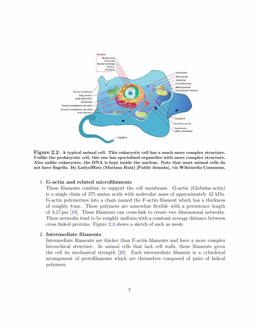
Figure 2.2: A typical animal cell. This eukaryotic cell has a much more complex structure.Unlike the prokaryotic cell, this one has specialized organelles with more complex structure.Also unlike eukaryotes, the DNA is kept inside the nucleus. Note that most animal cells donot have flagella. By LadyofHats (Mariana Ruiz) [Public domain], via Wikimedia Commons.

1. G-actin and related microfilamentsThese filaments combine to support the cell membrane. G-actin (Globular-actin)is a single chain of 375 amino acids with molecular mass of approximately 42 kDa.G-actin polymerizes into a chain named the F-actin filament which has a thicknessof roughly 8 nm. These polymers are somewhat flexible with a persistence lengthof 3-17 µm [19]. These filaments can cross-link to create two dimensional networks.These networks tend to be roughly uniform with a constant average distance betweencross linked proteins. Figure 2.3 shows a sketch of such as mesh.

2. Intermediate filamentsIntermediate filaments are thicker than F-actin filaments and have a more complexhierarchical structure. In animal cells that lack cell walls, these filaments giventhe cell its mechanical strength [20]. Each intermediate filament is a cylindricalarrangement of protofilaments which are themselves composed of pairs of helicalpolymers.

7

3. MicrotubulesMicrotubules are the thickest class of structural proteins. These are structures madeof α-tubulin and β-tubulin. This unit is 8 nm in length and has a molecular mass ofabout 100 kDa. The overall microtubule can have a mass of about 160 kDa/nm.

Figure 2.3: This sketch shows the mesh like structures generated through the cross-linkingof F-actin filaments. This gives a good approximation for the structure of cell cortex.

Obviously, cells are incredibly complex things. Simulating a full cell would be extremelydifficult, if not completely impossible. The way such an object reacts to stimuli would beimpossible to simulate regardless of how much computational power is available. Simpli-fications are needed to be able to simulate such systems. Fortunately, as we will see inlater chapters, the behaviour of the cell can be approximated. Thus cell behaviour can bestudied in silico and compared to experimental results.

2.2 Cell Division

Cell division itself is a highly complex process that differs between cells of different organ-isms[21, 22] and is controlled by many different conditions [23–26]. Furthermore, incon-sistencies can introduce many variations that further complicate the behaviour of cellularsystems. These variations may have useful effects such as morphogenesis [27–30] and detri-mental effects such as cancers or other diseases [31–33] when they occur erroneously.

Walther Flemming first observed cells in mitosis in the 1880s [34], and cell division beenan intense topic of research ever since. Much work has been invested into studying the

8

molecular mechanics of mitosis including what regulates it and which proteins participatein it [5]. He coined the term “mitosis” which comes from the Greek work for thread,mito, after noting the thread like structures of dividing cells. The process of mitosis isa multi-step process that depends on many factors within the cell and its environment.First the cell grows if there are enough nutrients in the system. Once it then reachesappropriate size, the internal mechanisms of cell division are started. This includes thereplication of DNA and the creation of proteins that structurally partition the cell into twodaughter cells. Cell mechanics ensure that mitotic cells have a roughly spherical shape[35,36], they define the division plane[5, 37, 38], and even govern the changes in the cell shapeby manipulating the cell cortex. The cells proliferate to create the various organs in thehuman body.

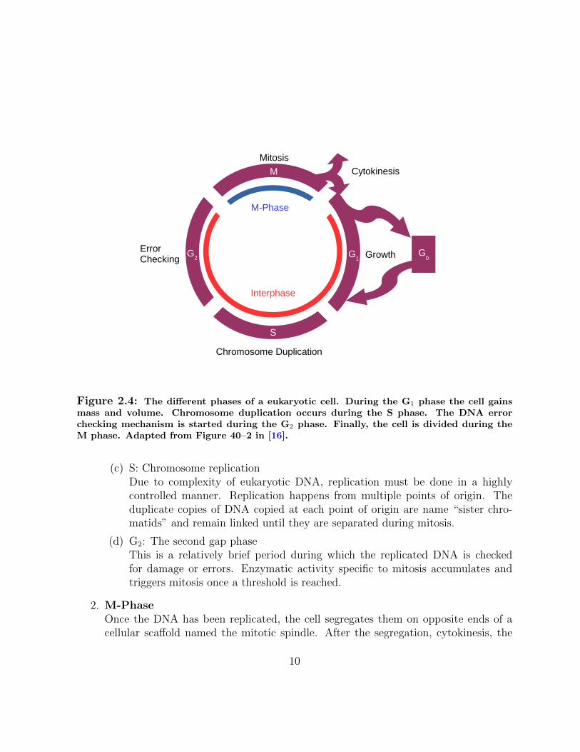
The cell cycle is the series of events that lead to duplication and replication of a cell.Figure 2.4 shows a typical cell cycle. The goal of the cell cycle is to produce two daughtercells that are accurate copies of the parent. There is a continuous growth cycle withaccompanying increase in cell mass and volume, and a discontinuous division cycle inwhich DNA is replicated and distributed to the daughter cells.

While bearing in mind figure 2.4, we can then see what the detailed steps involved incell division are. The cell cycle is divided into three phases[16, 39]: M-Phase, Interphase,and cytokinesis.

1. InterphaseThis is the part of the cell cycle in between subsequent mitosis events. The cells growand replicate their DNA in this phase which can further be divided into 3 steps:

(a) G1: The first gap phaseThis is the longest and most variable portion of the cell cycle. When cellsenter this portion of the cell cycle, they are normally half the size of theirparent cell. They grow to maturity during this phase. At the beginning of thisphase, all of the mechanisms that govern replication and division are halteduntil the restriction point. The restriction point is when the cell checks thesupply of nutrients before it starts the remaining steps before mitosis. Once itis determined that there is sufficient nutrient supply, the cycle continues.

(b) G0: Differentiation and growth controlAfter the organism has developed sufficiently, most cells differentiate into a newGo state and no longer divides. The cell is still highly active doing things otherthan division and can be motile as well. This state is not permanent, the cellcan reenter G1 phase to divide again.

9

G1

G1

S

G2

M

ErrorChecking

Mitosis

Chromosome Duplication

Growth G0

Cytokinesis

M-Phase

Interphase

Figure 2.4: The different phases of a eukaryotic cell. During the G1 phase the cell gainsmass and volume. Chromosome duplication occurs during the S phase. The DNA errorchecking mechanism is started during the G2 phase. Finally, the cell is divided during theM phase. Adapted from Figure 40–2 in [16].

(c) S: Chromosome replicationDue to complexity of eukaryotic DNA, replication must be done in a highlycontrolled manner. Replication happens from multiple points of origin. Theduplicate copies of DNA copied at each point of origin are name “sister chro-matids” and remain linked until they are separated during mitosis.

(d) G2: The second gap phaseThis is a relatively brief period during which the replicated DNA is checkedfor damage or errors. Enzymatic activity specific to mitosis accumulates andtriggers mitosis once a threshold is reached.

2. M-PhaseOnce the DNA has been replicated, the cell segregates them on opposite ends of acellular scaffold named the mitotic spindle. After the segregation, cytokinesis, the

10

process of cleaving the cell into two daughter cells begins. This phase proceeds infive steps.

(a) Prophase: Formation of the mitotic spindleA change in the properties of the cytoskeleton cause it to separate and form twopoles of the mitotic spindle.

(b) Prometaphase: Nuclear breakdownThe nucleus breaks down and the sister chromatids and begin to move towardsthe centre of cell roughly half-way between the two cell poles.

(c) Metaphase: Mid-point of the processAt this point the chromosomes are roughly halfway between the two cell poles.They form a collection of chromatids named the metaphase plate.

(d) Anaphase: Sister chromatid seperationThe chromatids separate and begin to move opposite spindle poles and thepoles themselves begin to move apart. The cell cortex is also activated to begincleaving the cell into two.

(e) Telophase: Nuclear envelope reformationThe separated chromatids are now enveloped in new nuclear membranes.

3. CytokinesisOnce all of the genetic information and organelles have moved into the regions of theparent cell, a contractile ring of protein fibers (actin and myosin) forms about theequator of the parent cell. The ring contracts, forms a cleavage furrow and pinches thecell into two daughter cells. Figure 2.5 shows the onset of cytokinesis. The contractilering continues to contract until the two halves of the parent cell are “pinched off” ofeach other. This process is a delicate balance between the internal pressure of thecell (aka the turgor pressure in plants and fungi) [16, 40, 41], the plastic nature ofthe cell membrane, and the forces of the cytoskeleton. It is theorized that similarmechanisms contribute to cell migration[37].

2.2.1 The Division Plane

The selection of the division plane is another interesting aspect of cell division. The divisionplane of the cell is simply the plane in which the contractile ring lies. Or in other words, itis the plane at which the parent cell is pinched off to make daughter cells. The orientationof cell the division plane is required to generate complex multi-cellular organisms[42].

11

Figure 2.5: After the chromatids have been correctly separated a the end of anaphase, acontractile ring of actin forms roughly halfway between the two cell poles during telophase.This concludes the activities of M-Phase. Cytokinesis begins with the protein ring contract-ing and ends when the two halves of the parent cell are pinched off of each other.

Orientation of the division plane can have significant bearing on development and celldifferentiation[43].

The selection of the cell division plane can vary from cell type to cell type. The shapeof the cell can affect division plane [42] in addition other factors such as the alignment ofthe molecular spindle [44]. There may be more than one force that act on the centering ofthe molecular spindle.

Given all of these factors that can affect the division plane orientation, we can look atwhat different division planes are possible and effects they may have. The first type ofdivision plane is selected by Hertwig’s rule, also known as the “long axis rule” [45]. Hertwigconcluded: “The two pole of the division figure come to lie in the direction of protoplasmicmass”. That is the mitotic spindle lies along the longest axis of a cell. Then, the divisionplane is chosen roughly mid-way, perpendicular to this axis.

In addition to reproduction where the cell is divided in to cell of equivalent size, it ispossible to have asymmetric division[30, 38]. In this case the one of the daughter cells issignificantly larger than the other[32, 35, 46, 47]. The division plane may depend on thealignment of the mitotic spindle, if the spindle is misaligned with respect to the axes of thecell, then the division occurs such that one daughter is smaller than the other. However thisis not always the case, sometimes mitosis begins in a symmetric way, then at some pointafter the formation of the cleavage furrow, one half the cell expands and the other contracts.A consequence of asymmetric cell division is that the daughters may receive different kindsof intrinsic cell-fate determinants which play a role in differentiation[47]. Some kinds of

12

stem cells are known to differentiate from reproducing through asymmetric cell division[48],and producing new cell types. We will see later that in the 3D model developed in thisthesis, the division plane is set randomly and symmetrically (see Section 5.3 and figure 2.6).Other division planes are planned for the future. In the 2D model on which the 3D modelis based, introduced by Mkrtchyan et al. [15, 49], all three division schemes were studied.So the model presented in Chapter 5 is amenable to modelling different division planes.

Figure 2.6: Division planes showing symmetric and asymmetric division. The bold orangeline is the mitotic spindle. The orange dashed line shows the symmetric division plane. Thepurple dashed line shows an example of an asymmetric plane line.

2.2.2 Inter-Cellular Adhesion

The adhesion forces between cells play an important role in their interactions and be-haviour [50–55]. Cells may adhere to substrates, the extracellular medium, or other cells.The complex structures of cell membranes make it difficult to describe accurately. Theremay be two sources for the adhesion interaction between cells: van der Waals forces, andsite specific adhesion mediated by Cell Adhesion Molecules (CAM) [50]. Variation in celladhesion is known to have effects on the geometry and function of tissues [54, 56]. At longerranges, the adhesion is caused by van der Waals interactions and electrostatic interactionsbetween lipids with charged head groups. As membranes of different cells come into closeproximity with each other, steric hindrance and thermal undulations of the membranescause repulsion.

Stronger adhesion interactions occur through specific interaction sites between CAMs.CAMs are molecules embedded in the cell cortex that interact with CAMs of other cellsor the extracellular [50]. These CAMs may be spread evenly over the surface of cells or atspecific junctions that induce some control over the structuring of tissue [50].

13

Due to the complex nature of cell behaviour, especially cell reproduction, there is a needfor theoretical frameworks to study cells and provide predictions. Quite a few models havebeen proposed to meet this need[15, 34, 57–64]. Some of these are described in Chapter 3.

2.3 Molecular Dynamics

Molecular Dynamics (MD), is a very powerful and highly used method to model matter atthe molecular level. With this method, we can simulate systems in states of equilibrium andnon-equilibrium [65]. Over the past several years, many software packages have emergedthat can run MD simulations of very large systems efficiently. These include packagessuch as the Large-scale Atomic/Molecular Massively Parallel Simulator (LAMMPS) [66],DLPOLY [67], the GROningen MAchine for Chemical Simulations (GROMACS) [68], theNAnoscale Molecuar Dynamics (NAMD) [69], the Extensible Simulation Package for Re-search on Soft matter (EXPResSO) [70], the Molecular Modelling ToolKit (MMTK) [71],and the Highly Optimized Object-Oriented Molecular Dynamics (HOOMD-blue) [65].Most of these packages support multithreading on multi-core CPUs and parrallelizationacross multiple computational nodes with multiple CPUs. Some of these packages such asGROMACS and HOOMD-blue support acceleration on GPUs as well.

All of the packages above are fundamentally alike in that they use the same algorithmsthat have were first developed in the 1950–1970 in theoretical physics; these methods havebeen evolving ever since. When first developed, these methods were primarily used tostudy simple atoms[72–75].

One of the very first MD simulations was run by Alder and Wainwright in 1957[72]that used a hard sphere model where all atoms interacted through perfect collisions andstudied their phase transition. Later, Rahman applied a continuous potential that madethe atoms behave more realistically [73]. Rahman showed that this method could reproducethe properties of Argon at 94.4 K. The very first protein was first simulated with MD in1977 by Karplus al. [76]. The Karplus group simulated the dynamics of Bovine PancreaticTrypsin Inhibitor (BPTI). These simulations were all conducted with less than 1000 atoms,and since then the number of atoms that are routinely simulated has grown rapidly to thepoint that simulations with 104–106 atoms have become commonplace[8].

Furthermore, the very first simulations could only simulate on the order of 10’s of ps at atime due to limitations of computational power. Nowadays it is common to run simulationsup to the µs range with simulated domain sizes on the order of 1 µm3 thanks to the vastimprovements in computational power and methodological techniques. There has been a

14

great deal of work in studying the properties of, among other systems, lipid aggregates[9,10, 77], lipid monolayers[78, 79], bilayer pore formation [80], protein binding [81, 82], andenzyme activity [83].

Despite these vast improvements, there is still a never ending demand for larger simula-tions that are run for longer. Therefore, there is a great deal of interest for parrallelizationof MD codes over multiple Central Processing Units (CPUs) and Graphics ProcessingUnits (GPUs). This demand coupled with the fact that access to supercomputers withmany CPUs is difficult and expensive has increased the interest in GPU acceleration whichare cheaper to use and easier to operate. The technology that has been developed to runMD over multiple CPUs can be reused to run on multiple GPUs if needed.

The aim of MD simulations is to compute macroscopic behaviour form microscopicinteractions[84]. When the macroscopic behaviour can be reproduced computationally bysimulating microscopic systems, the simulations can be used to study the macroscopicsystems computationally. MD furnishes the scientist with the capacity to study real andtheoretical system as well.

2.3.1 Methodology

A simulation method, henceforth called the model, needs to be both correct as far as itsresults go and also needs to be tractable. That is, it must use minimal resources (memoryand/or processing power). The most expensive part of any model is the complexity ofthe interactions between the particles in a system described by a potential energy equa-tion. These equations are approximations of the fundamental laws of physics that governreal atoms. The approximations are made due to some assumptions that simplify theinteractions somewhat.

With elementary mechanics, the force on a particle i is defined as function of thepotential energy that a particle feels, U as shown in (2.1).

Fi = −∇U (2.1)

If U is defined correctly, the force on any particle can be calculated. When definingU , it must be first decided what interactions will be modelled. A valid simulation iscompletely dependent upon the accuracy of the potential energy landscape of the system.Simultaneously, the potential energy functions must remain tractable to not overwhelmcomputational resources. U is broken down into a sum of different potential functions Uintdepending on the type of interaction,

15

U =∑int

Uint. (2.2)

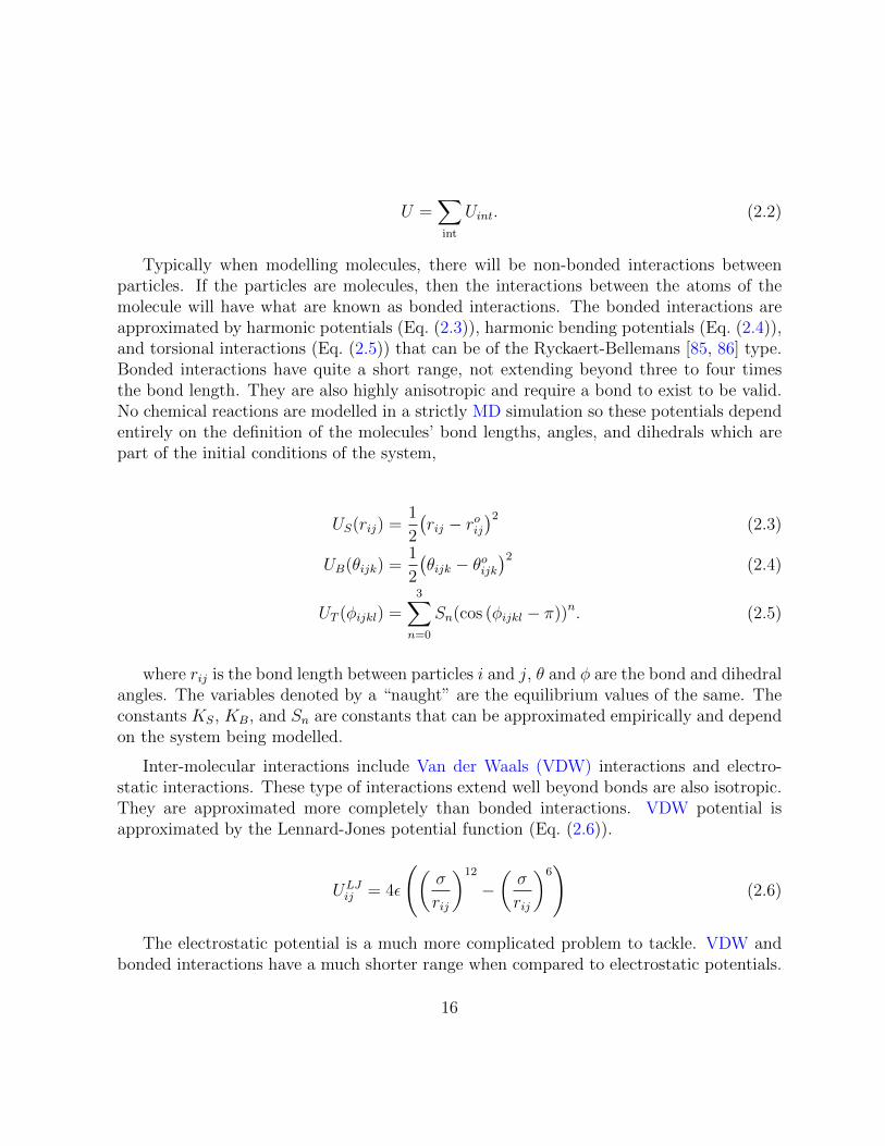
Typically when modelling molecules, there will be non-bonded interactions betweenparticles. If the particles are molecules, then the interactions between the atoms of themolecule will have what are known as bonded interactions. The bonded interactions areapproximated by harmonic potentials (Eq. (2.3)), harmonic bending potentials (Eq. (2.4)),and torsional interactions (Eq. (2.5)) that can be of the Ryckaert-Bellemans [85, 86] type.Bonded interactions have quite a short range, not extending beyond three to four timesthe bond length. They are also highly anisotropic and require a bond to exist to be valid.No chemical reactions are modelled in a strictly MD simulation so these potentials dependentirely on the definition of the molecules’ bond lengths, angles, and dihedrals which arepart of the initial conditions of the system,

US(rij) =1

2

(rij − roij

)2(2.3)

UB(θijk) =1

2

(θijk − θoijk

)2(2.4)

UT (φijkl) =3∑

n=0

Sn(cos (φijkl − π))n. (2.5)

where rij is the bond length between particles i and j, θ and φ are the bond and dihedralangles. The variables denoted by a “naught” are the equilibrium values of the same. Theconstants KS, KB, and Sn are constants that can be approximated empirically and dependon the system being modelled.

Inter-molecular interactions include Van der Waals (VDW) interactions and electro-static interactions. These type of interactions extend well beyond bonds are also isotropic.They are approximated more completely than bonded interactions. VDW potential isapproximated by the Lennard-Jones potential function (Eq. (2.6)).

ULJij = 4ε

((σ

rij

)12

−(σ

rij

)6)

(2.6)

The electrostatic potential is a much more complicated problem to tackle. VDW andbonded interactions have a much shorter range when compared to electrostatic potentials.

16

Therefore, a much larger number of particles (close to infinity) have to be simulated inorder for the simulation to be realistic. This is, of course, impossible to do. This issue alsoaffects other non-bonded interactions for the same reason of wanting to simulate systemscomparable in size to experimental systems with many moles of particles in a reactionvessel.

Figure 2.7: Sketch of periodic boundary conditions. A much larger system is created byperiodic images of the simulated system. The virtual particles interact with the particles nearthe boundary of the simulation box. As particles exit the simulation box, a copy replacesit on the opposite side. Particles can interact with other particles and virtual particlesdepending on the distance between them.

These problem of system size is alleviated with Periodic Boundary Conditions (PBC),see figure 2.7. PBC make the simulation of smaller microscopic systems resemble largermacroscopic systems more closely. PBC introduce a periodicity into the system that is onlyvalid for crystalline systems. This artifact introduced by PBC is removed by the minimumimage convention[87].

With this setup, the electrostatic potential energy function can be formulated in atractable way. Due to their long range, electrostatics have to be modelled using morecomplex methods. To consider all of space surrounding a particle, Ewald sums are usedwhere the electrostatic energy is calculated in Fourier space[88–90]. There are three popular

17

algorithms that implement Ewald sums: Particle Mesh Ewald (PME)[88], Smooth ParticleMesh Ewald (SPME)[91], and Particle Particle Particle Mesh (P3M) [92]. Eq. (2.7) definesthe total electrostatic energy in a system of N Coulomb point charges.

E =1

2

N∑i,j=1

∑nεZ3

qiqj|rij + nL|′

(2.7)

where rij is the vector between particles i and j, L = diag(lx, ly, lz) is a diagonal matrixwith sidelengths lx, ly,lz, n indexes the surrounding periodic cells, and the ′ indicates thatthe calculation is ignored for i = j and n = {0,0,0}.

Equation (2.7) decays very gently over r, so a direct calculation is not feasible. ThePME, SPME, and P3M are some efforts to solve this problem. Readers are referred to [90,93, 94] for more details about electrostatic force-field calculations. Due to the complexityof these potential functions, the simulations may require a large amount of computerresources—even more is needed for simulating macromolecules. This problem is solved bycoarse-graining [95].

The simulations are often times run with the molecules being described at the atomiclevel. This can be prohibitively expensive. Coarse-graining is built upon the assumptionthat the internal dynamics interatomic interactions are of less importance than intermolec-ular interactions of large macromolecules [95]. Groups of atoms are grouped into beads thatthen interact with each other. There are a large number of coarse-graining methods[96–100] that have been implemented in the aforementioned software packages.

Now that the interparticle interactions are defined, the next step is to calculate andupdate the particle positions and velocities. As part of the initial conditions, the particlepositions are chosen randomly and given random distributions. The positions are takenform a uniform distribution and velocities are chosen from the Maxwell-Boltzmann[84]distribution, shown in Eq. (2.8), to reach equillibrium quickly,

p(vi) =

√mi

2πkBTexp(−miv

2i

2kBT). (2.8)

Equation (2.1) can be rewritten into a differential form,

md2xi

dt2= −∇U(xi) (2.9)

18

which will have to be solved numerically. The velocity Verlet [101] algorithm is usedthanks to its symplectic nature symmetry under time reversal [101, 102]. Equations (2.11)and (2.10) define the math behind velocity Verlet,

ri(t+ ∆t) = 2ri(t)− ri(t−∆t) +Fi(t)

mi

·∆t2 +O(∆t4) (2.10)

vi(t) =ri(t+ ∆t)− ri(t−∆t)

2∆t+O(∆t2). (2.11)

Notice that in all of the equations described above, it seems that they can be calculatedsimultaneously for each particle. The calculation of, say, the force on a certain particledoes not depend on the forces on the other particles in the system. This can be takenadvantage of any the calculation may be parrallelized to be carried out simultaneously onmultiple cores and CPUs. Due to network latency, unfortunately, there are a diminishingreturns associated with increasing the number of CPUs. The number of CPUs used has tobe balanced with the overall performance (measured in steps/day or ns/day) of the simu-lation. The latency problem can be avoided by using GPUs. GPUs can run many threadssimultaneously, and deal with intercommunication without high latency networking. Manyof the MD software packages mentioned before already support acceleration on GPUs.

Finally, note that the MD done for this thesis is slightly different in that it does notmodel the interaction between atoms and molecules. Essentially, only the aspect of inte-gration used in MD will be used for modelling cell dynamics. This is done by definingcustom, and much simpler, force fields that operate on mass points that are much moremassive than single molecules. This is described in detail in Chapter 5.

19

Chapter 3

Some Cell Modelling Techniques

As discussed in previous chapters, cell behaviour is extremely complex and depends onmany factors. The behaviour is interesting because its responses to chemical and physicalstimuli is what leads to development of complex multi-cellular living organisms. Much hasbeen learned through the traditional experimental nature of cell biology. Much progresshas been done since Flemming first described mitosis in the late 19th century [34].

Cell biologists have learned a great deal of regarding the operation of the internalcomponents of the cell. Such as the role of mitochondria in energy production and cellularmetabolism, the photosynthesis function of chrolophyl in plant cell, the conduction ofelectrical impulses through axons in nerve cells, etc [16, 18]. The vital behaviour of groupsof cells is also a vibrant topic of inquiry [103–105]. Not only for scientific curiosity, but alsoto more practical ends such as understanding the mechanisms of disease or decay due to oldage. Naturally, there is a need for multidisciplinary research activities to full understandsuch phenomena.

Any complex phenomenon that is difficult to describe analytically, i.e. anything thatis even a little more realistic than spherical cows in a frictionless vacuum, is an attractivetopic for the development of computational models that allow us to run simulations thatcan accurately simulate that behaviour. The models that arise from such analysis canthen be used as either a basis for experimental design, as an augmentation to alreadyavailable experimental evidence, or even as a cheap sandbox to create strange environmentsand stimuli that are difficult to create in the lab. Thus, many computational techniqueshave been developed to study cells. This chapter attempts to summarize some of thesetechniques.

When considering cell behaviour, it is possible to have multiple types of models that can

20

be used. The field of mathematical biology encompasses a number of so–called continuummodels which are ones in which the behaviour of cells is modelled using mathematicalequations that link certain behaviours to parameters related to the cell type or environment.This method produces a set of coupled differential equations that can be solved and theirsolutions compared with experimental data. The problem with these techniques is theysacrifice the vast majority of the properties of the cells themselves in order to elucidate somemacroscopic “emergent” property. This is not always possible as inter-cellular interactionscannot always be approximated fully [106].

The other type of models are those that consist of cells that are treated as individualcells. In most cases, the cell is modelled as a closed shape that interacts with its surround-ings in a particular way. The nature of this interaction, of course, depends on the modelitself. The advantage with these methods is that the individual behaviour of the cellsthemselves can be studied and observed computationally. Naturally, the cost of computa-tions is significantly higher with these type of models. Despite the increased granularity,or resolution, of these types of models, many approximations have to be made regardingcell structure itself. Additionally, these models will abstract away all of the minute in-termolecular interactions that intercellular interactions are based on. It is also possibleto create hybrid models that are based on both of these principles with discrete elementsbeing affected by continuous functionals [107].

The model that is presented in this thesis is based on previous work by Karttunenand Astrom, who designed the basic principles in 2006 [14], and the work of Mkrtchyan etal. [15, 49] that was used to study epithelial packing in 2014. The 2D model is describedin Section 3.3

3.1 Mathematical Biology

The first kind of models that can be used to study cell behaviour are those that willbe referred to as either mathematical models, these are the kind that simply reduce cellbehaviour into mathematical formulations that apply to on specific aspect of cell behaviour.This techniques are placed under the umbrella of Mathematical Biology and can be thoughtof as continuum models.

In this class of techniques, differential equations are derived from principles observedexperimentally or from first principles —biological first principles. Unfortunately, thereis a difficulty in defining principles such as the rules of equilibrium or conservation thatgovern cell behaviour[108]. This is due to the non-linear nature of the interactions between

21

cells, i.e. the outcome of interactions of a cell with its neighbours is not always a linearsum of each individual interaction with each individual neighbour [109].

Therefore, it is rarely biologically sound to try to show some macroscopic propertiesfrom first principles [106]. Nonetheless, these methods can be very useful to study systemsthat are at least temporarily in the valid domain of applicability of a specific model.

In general, models of this type have been developed to study many various cellularphenomena [108, 110, 111] such as: cell-cycle control, cell death, cell differentiation, cellaging and renewal, and the same for cancer cells. Or sub-cellular phenomena such as:DNA control (Transcription, Replication, Repair), or endocytosis[112]. Readers interestedin other aspects of this field are referred to Refs. [106, 108, 110, 113–115].

3.1.1 Models of Cell Population Dynamics

As an example of mathematical biology, consider the study of population dynamics. Theprogression of cell growth over time has always been an important area of study. Firstly,measuring the population of a culture and observing its trend are fairly simple procedures,compared to other more complex experiments, so it can be done relatively easily. Thetrends in the number of cells in a culture over time can easily be observed, and be plotted.This type of graph will be called the population curve or population trend line hereafter.The cells of different organisms grow at different rates and with different kinds of trends.Anomalies in population trends can be linked to illness [116]. The population curve canalso differ greatly within the same species depending in what stage of life that organismis in (development, reproduction, death, etc.). Growth curves with remarkably similarproperties can be found in the progression of many quantities such as the height of ahuman, or population of most organisms. These growth curves tend to be sigmoidal andcan even describe quantities such as dose-mortality relations [117].

While making some simple assumptions, one can very easily derive the population curveof an ideal system where nothing limits cell growth at all. At one instance in time, somefraction r of cells will divide, so the rate of change of the number of cells N will be givenby (3.1). Which can trivially be solved to give (3.2) where No is the initial number of cells.

dN

dt= rN (3.1)

N(t) = Noert (3.2)

22

The function in (3.2) is called an intrinsic growth trend, it describes the populationgrowth under ideal conditions where each individual has complete access to nutrients anddoes not perish. Unfortunately, or fortunately depending on perspective, this is not thecase. The conditions for growth are far from ideal, one can even say that it the world ishostile of growth. There are many factors that limit growth rate such as competition withother cells for nutrients, the limited lifetime of cells with an associated death rate, thethreat of disease and/or predators, etc. A more complex trend is normally observed. Thisis where we shift to looking at sigmoidal functions.There have been number of functions[116–118] that are known to follow this behaviour:

• Intrinsic Growth [119]N = Noe

kt, (3.3)

• The logistic function [117]

N =Nmax

1 + be−kt, (3.4)

• The Gompertz function [120]

N = Nmaxe−be−kt

. (3.5)

These models are not only valid to study the cell number over time, but can also beapplied to other observables such as average size or weight[116, 118]. Typically in suchsystems, growth starts at population of zero (or some small value close to zero) at t = 0,accelerates to a maximum (µm) after a lag time (λ), finally the growth rate drops to zeroagain asymptotically at a maximum population A [117].

In 1981, Schnute generalized all of the growth models shown above, including someother more complex ones, into special cases of a universal growth model[116]. Zwieteringet al. [117] did a study that compared various special cases of the Schnute model [116] andshowed that they can produce good fits to the population trends of various bacteria, wherethe parameters µm, λ, and A were found with nonlinear fitting.

3.1.2 Continuum Models of Cell Behaviour

Local interaction functions are used to develop these type of models[51, 121–123]. From amathematical perspective, these models are not much different from the models in mathe-matical biology. The microscopic interactions of cells are abstracted into functional forms

23

which may describe parameters such as density, growth rate, death rate, inter-cellular in-teraction strength [122], or interaction strength with the medium [109]. Unfortunately,this kind of modelling cannot take into account of all the minute interactions between cellmembranes, and therefore are not always ideal for simulating cell behaviour.

Somewhat like in many-particle physics, all of the individual cells are modelled withsome continuous parameter like density. Then, spatiotemporal equations of motions arederived that describe the dynamics of a continuum of cells [115, 124]. This method yieldsthe dynamics of the total population as whole and individual behaviour is neglected. Con-tinuum models have been used to study a variety of phenomena such as tissue deformabil-ity [51], tumour growth [121], viscosity of tissues [122], and anisotropic tissue growth [123].While the results of computational studies have proven favourable, their limitations remain.Continuum models cannot take the mechanical interactions between cells at the cellularscale of size. Methods that can model individual cells are needed to fully understand cellbehaviour.

3.2 Discrete Cell Models

Now we take a look at some models that implement cells as individual entities that interactwith their surroundings, much like real cells. These models can be more computationallyexpensive, however they allow us to study different aspects of cell behaviour at a lowerlevel without forgoing any of the small interactions between cells. It is possible to havemodels that simulate cells as either two dimensional or three dimensional objects. Twodimensional models are cheaper computationally though they do not possess the ability tomodel the full breadth of cell behaviour directly as they are missing the third dimension.Three dimensional models can capture cell behaviour more fully, but are computationallyvery expensive. More generally, cell models that simulate single cells can also be namedagent-based methods.

3.2.1 Delaunay Object Dynamics

Delaunay Object Dynamics (DOD) is a three dimensional technique where each cell ismodelled as a three dimensional, elastic, and adhesive Voronoi cells [64, 124–126]. A cell isdescribed as a three dimensional polygon that is constructed with Delaunay triangulation.Readers interested in the details of Delaunay triangulation are referred to [125, 127, 128].Each face and edge of each cell is then modelled with damped Newtonian Mechanics [125].

24

The Delaunay triangulation used in this method is slightly varied form regular Delaunaytriangulation and is termed weighted Delaunay triangulation [64, 129]. To put it simply,Delaunay triangulation is method of triangulation for a set of points that obeys the De-launay Condition [125, 130]. The Delaunay condition is that the circle circumscribing anytriangulation must not contain any other points. Figure 3.1 shows a Delaunay triangulationof a random set of points.

Figure 3.1: Here the Delaunay triangulation of two dimensional cells is shown. The dashededges belong to Delaunay simplices, the solid line is the Voronoi region corresponding to themiddle cell. The overlapping circles represent the weighting of the triangulation. Reprintedwith permission [124] c© 2005 American Physical Society.

The Delaunay triangulation describes the topology of the surroundings of the cell andhow it is positioned in space with respect to its neighbours. This way, the triangulationdescribes the distances between cells very well. The dual graph of Delaunay triangulationis the Voronoi tessellation of the same set of points [131]. The Voronoi regions, shown inFigure 3.1 describe the shape, contact surfaces, and sizes of the cells in the system [64].Cell division, death, or flux changes the triangulation by adding, removing, or changingthe positions of points in the system. As the points change the Delaunay and Voronoigraphs change accordingly.

The forces between cells are caused by interactions occurring on the surfaces of theVoronoi cells are modelled along the Delaunay triangulation simplices [64, 124, 126]. TheDOD force-field contains terms for active forces that are generated by the exertion of

25

cytoskeleton on the cells’ surroundings, and passive forces that are a result of the cells’interactions with their neighbours. The passive forces model cell elasticity and adhesion.Lastly, the forces are damped by a drag forces on all cells that embody the interaction ofthe medium with the cells.

DOD has been used to study the proliferation, death, and behaviour of lymphoidcells [64], tumour cell reaction to changes in nutrient levels [124]. DOD is also gener-ally applicable to tissue organization [64], and cell migration [132].

3.2.2 The Cellular Potts Model

Physicists have been for a very long time modelling and analyzing problems which exist atmany different scales of space and time, so called multi-scale problems. The mechanismsthat control tissue organization depend on the local intercellular interactions between eachcell and its neighbours. The Cellular Potts Model (CPM) is a lattice based model that thatcan be used to understand the factors at the cellular scale that affect tissue organization [60,133].

For many decades, physicists have been developing models that apply to very difficultmulti-scale problems. It is often possible to find some already existing model used for someunrelated science in the wild that can be applied to a new problem at hand. The CPM isone such model that was developed by Glazier and Graner[134, 135]. The model originallydeveloped in the field of solid-state physics to study ferromagnetism. This model is alsocalled the Glazier-Graner-Hogeweg[60] model.

The CPM is based on the Potts model that was developed by R.B Potts under thetutelage of C. Domb in the early 1950s[136]. Potts proposed this model as a part of hisPhD thesis. It is a generalization of the Ising model[137] where instead of consideringtwo possible states, such as for example atomic spin states -1 and +1, the Potts modelconsiders any number of states. See the review by Wu[138] for a more detailed descriptionof the Potts model.

Much like the Potts model, the CPM is a lattice model at heart. That means thateach cell no longer is its own entity, but collection of grid points, which may be pixels orvoxels. These collections grid points are then treated individually. Graner and Glazier firststudied cell sorting using this method [135], but it is possible to study other phenomenasuch as cell migration[62], and morphogenesis[139]. The lattice grid may be cubic orhexagonal. The basic idea in this type of modelling is too minimize the energy undercertain imposed fluctuations. The cell is modelled as a more-or-less deformable object and

26

its shape is affected by both internal and external stimuli. The parameters of the modelcan be mapped to the physical and biological properties of real cells.

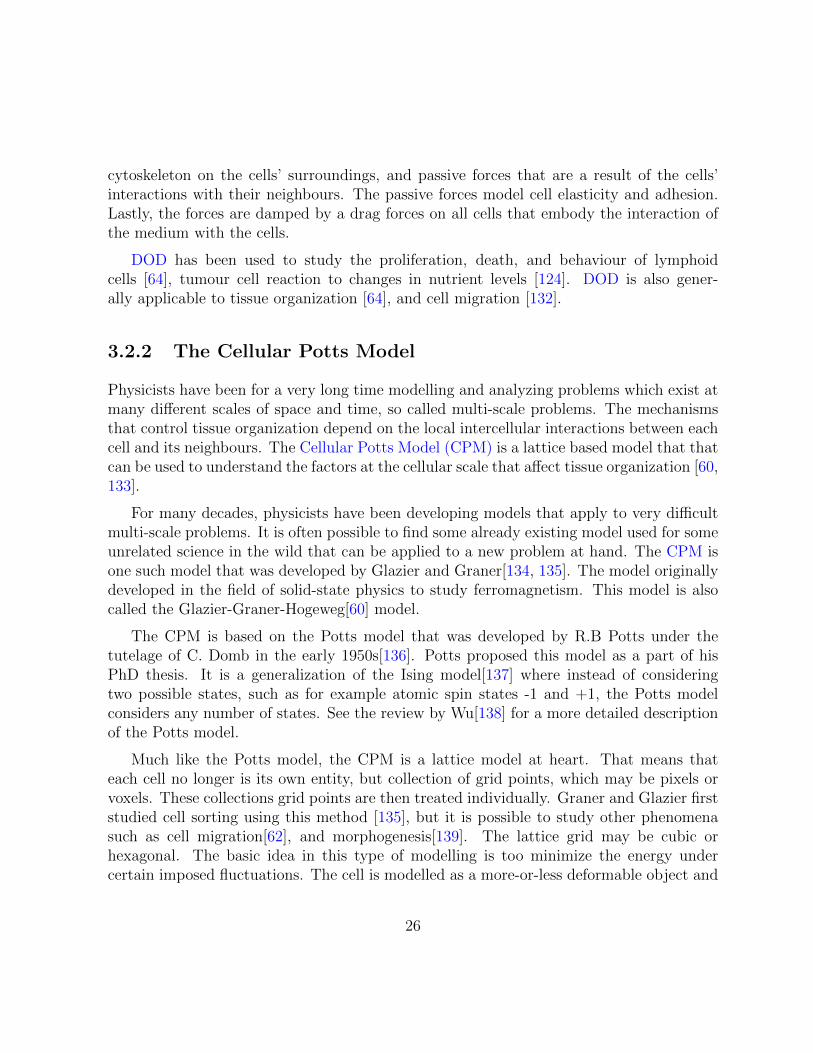
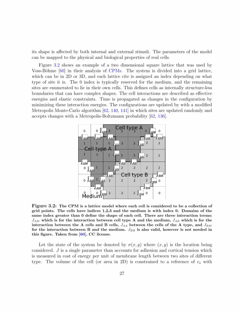
Figure 3.2 shows an example of a two dimensional square lattice that was used byVoss-Bohme [60] in their analysis of CPMs. The system is divided into a grid lattice,which can be in 2D or 3D, and each lattice cite is assigned an index depending on whattype of site it is. The 0 index is typically reserved for the medium, and the remainingsites are enumerated to lie in their own cells. This defines cells as internally structure-lessboundaries that can have complex shapes. The cell interactions are described as effectiveenergies and elastic constraints. Time is propagated as changes in the configuration byminimizing these interaction energies. The configurations are updated by with a modifiedMetropolis Monte-Carlo algorithm [62, 140, 141] in which sites are updated randomly andaccepts changes with a Metropolis-Boltzmann probability [62, 136].

Figure 3.2: The CPM is a lattice model where each cell is considered to be a collection ofgrid points. The cells have indices 1,2,3 and the medium is with index 0. Domains of thesame index greater than 0 define the shape of each cell. There are three interaction terms:JAM which is for the interaction between cell type A and the medium, JAB which is for theinteraction between the A cells and B cells, JAA between the cells of the A type, and JBM

for the interaction between B and the medium. JBB is also valid, however is not needed inthis figure. Taken from [60], CC license.

Let the state of the system be denoted by σ(x, y) where (x, y) is the location beingconsidered. J is a single parameter than accounts for adhesion and cortical tension whichis measured in cost of energy per unit of membrane length between two sites of differenttype. The volume of the cell (or area in 2D) is constrained to a reference of vo with

27

compressibility κ−1. ∆E is the energy difference between the two states. Equation (3.6)shows the probability distribution for accepting or rejecting updates,

P (∆E) =

{1 if ∆E ≤ 0

e−∆ET if ∆E > 0.

(3.6)

Where T represents the average fluctuation in the boundary of each cell. Normally, oneMonte-Carlo step (MCS) is an attempt to update each lattice site. Equations (3.7), (3.8), (3.9),(3.10) show how the energy of σ may be defined. Echem is the contribution to the energycoming from motile forces that point along the direction of cell polarity ni with fieldstrength µi.

The energy of any given pixel of a cell is given by

E = Eadh + Evol + Echem, (3.7)

whereEadh =

∑k,l

Jkl (1− δk,l) (3.8)

is an approximation of the intercellular interaction between cells, J is related to membranetension and differs depending on what two cells are being considered (JAB, JAM , JAA inFigure 3.2), k, l index the neighbouring pixels. δk,l is 1 if the pixels k, l belong to the samecell, and 0 otherwise.

Evol =∑i

1

2κ(vi − vo)2 (3.9)

is the energy needed to deform a cell, where v0 is the cell volume (area in 2D) at equilibrium,κ−1 is the cells compressibility, and vi is the instantaneous cell volume.

Echem =∑i

−µini · ri, (3.10)

is the energy resulting from motile forces along polarization vector ni, with magnitude µi.ri is the location of the cell’s centre of mass.

CPMs have been used to study a wide variety of cellular phenomena, especially cellsorting [134, 135, 142, 143], cell migration [62, 144], and chemotaxis [145, 146](cell motionin reaction to chemical gradient).

However, it is clear that the interactions between cells in CPM models do not take intoaccount any mechanical interactions between cells. While the resultant motion of cells dueto energetically unfavourable conditions can be correct, the mechanical interactions of cellsplay a vital role in their behaviour [54, 56].

28

3.2.3 Topological Models

This class of models are based on the work of Matella and Fletterick that they did inthe 1980s[147–149]. These models are inherently two dimensional and rely on graphs ofadjacent cells, much like DOD (see Section 3.2.1). In topological models, the cells aretriangulated such that they always meet at corners with two neighbouring cells [149] attrivalent junctions. The resultant arrangement is intentional because it was observed thatcells in planar systems favoured hexagonal packing[15, 49, 56, 61, 150–152]. The dual mapof the trivalent junction describes the adjacency of cells.

The dynamics of the cells are simulated by manipulating the map structure to introducecell division, growth, movement, adhesion, differentiation and death [149]. Cell divisionis simulated by introducing new edges that divide a parent cell into fairly symmetricdaughters. Cell growth is simulated by systematically increasing the size of cells. Cellmovement is done by exchanges in adjacent cells. Differentiation is done by subtly changingparameters of some of the cells so that their behaviour is slightly different. And finally celldeath is simulated by removing some edges of the dying cell until it finally disappears.

3 4 5 6 7 8 9Number of neighbours

0

10

20

30

40

50

Fract

ion (

%)

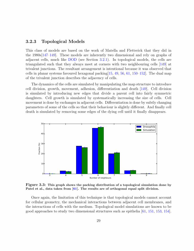
DrosophilaSimulation

Figure 3.3: This graph shows the packing distribution of a topological simulation done byPatel et al., data taken from [61]. The results are of orthogonal equal split division.

Once again, the limitation of this technique is that topological models cannot accountfor cellular geometry, the mechanical interactions between adjacent cell membranes, andthe interactions of cells with the medium. Topological model simulations are known to begood approaches to study two dimensional structures such as epithelia [61, 151, 153, 154].

29

However due to the assumptions made about the packing of cells, these models cannot beapplied to simulate three dimensional tissue, or tissue that is not necessarily hexagonal.

Consider the results shown in Figure 3.4 and Figure 3.3. The topological simulationthat was run by Patel et al. [61] produced the correct packing distribution of epithelialcells. But in Figure 3.4, we clearly see that the mechanics at the cellular level are notnecessarily correct.

Figure 3.4: Left: The approximate polygonal topology of the epithelium the Drosophilamelanogaster (fruit fly) wing disc as measured by Patel et al. [61]. Right: The topologicalmodel that was used to simulate the wing disc, as simulated by Patel et al. [61]. Dark bluecells have four neighbours, blue have five, green have six, orange have seven, and maroonhave eight. Even though Patel et al. ended up with the correct distribution of cell grouping,the model cells themselves do not arrange themselves like real cells. c© 2009 Patel et al.,CC license.

3.2.4 Vertex Models

Vertex models are a made of sub-cellular particles that are bound in tightly bound clouds,developed by Newman[63]. Each cell is represented by a cloud of mass mounts that areheld together with strong intracellular Morse potentials [63, 155], weak Morse potentialsare used for inter-cellular interactions (Eq. (3.11)),

V (r) = Vo exp(−r2

ζ21)− Uo exp(−r

2

ζ22), (3.11)

30

where Vo, Uo, ζ1, ζ2 determine the strength of adhesion and repulsion. This model canbe used to study cell reproduction in two and three dimensions.

3.3 Two Dimensional Cell Dynamics

The model that is described in this work is a three dimensional version of one that was firstdesigned by Karttunen and Astrom in 2006 [14]. Later, in 2014, Mkrtchyan, Astrom, andKarttunen expanded upon the model by adding modes of cell growth and division[15, 49].Since the model is two dimensional, epithelial cell packing seemed like an obvious targetfor model validation. They saw that their model could accurately reproduce the packingof the Drosophila wing disc[15, 49].

To summarize, the new model is a single-cell based mechanical model with which ac-counts for cell cortex contractility, and cell-cell adhesion[15, 49]. Each cell is a closedloop of mass points, and the mass points interact with each other in a force field thataccounts for bonding interactions between neighbouring mass points in the same cell, ad-hesive interactions with neighbouring cells, and intercellular friction. Each cell is assignedan internal pressure which controls the cells’ growth. Mitotic cells are known to grow byinternal pressure [35, 37], which makes the driving force behind growth biologically sound.Furthermore, the physical properties of tissue, and the effects of division on the same, canbe controlled at the cellular level. The system allows for spontaneous cell rearrangementsand movement without the need for stochastic laws.

3.3.1 Intracellular forces

A cell is represented by a loop of springs connected at mass points. This structure wasoriginally suggested by Astrom and Karttunen in their work on cell aggregation in confinedspaces[14]. Tension forces operate on each mass point through spring interactions withneighbouring mass points. Figure 3.5 shows the tension and pressure forces operating oneach mass point.

Spring forces of adjacent mass points balance the internal pressure force. With this,the forces acting on a mass point can be denoted as

Fcelli = σiηi − σi+1ηi+1 +

Pl

2(νi + νi+1) , (3.12)

31

Figure 3.5: The two dimensional model that was introduced by Mkrtchyan et al. [15,49]. Cells grow by gradual increase in their internal pressure. When a cell is divided, newmass points are added along the division line. The division line can be symmetric random,orthogonal, or asymmetric.

where η, ν are the tangential and normal vectors respectively, and σ is the tension forcedefined as σi = Kspr(l− lo), l and lo being the equilibrium and instantaneous spring lengthsrespectively. All of the springs are given the same spring constant Kspr

i ≡ Kspr, but thiscondition can be lifted.

3.3.2 Intercellular Forces

The force-field also defines inter-cellular forces in a two dimensional tissue. Mass pointsof different cells experience repulsion (Eq. (3.13)), adhesion (Eq. (3.14)), and intercellularfriction (Eq. (3.15)). For all of the following equations, i indexes the mass point beingconsidered and j indexes mass points belonging to other cells,

Frepij =

{−Krep(Rrep

c −Rij)Rij if Rij < Rrepc

0 otherwise.(3.13)

The mass points repulse if they are within Rrepc of each other. The repulsion force

should balance the pressure force that pushes all mass points outwards towards the masspoints of other cells, so the repulsion spring is set as Krep ≈ KsprPl.

Intercellular adhesion maintains tissue integrity. Real cells adhere to each other throughadhesive molecules[156, 157], this behaviour is emulated by this model by including attrac-

32

tive intercellular forces. Each mass point acts as a site for adhesive interaction. All sitesare assumed to have the same adhesion strength Kadh

ij = Kadh. The adhesion force isdefined in Equation (3.14) as

Fadhij =

{Kadhij

(Radhc −Rij

)Rij if Rij < Radh

c

0 otherwise,(3.14)

so that mass points within the attraction range, Radhc , attract each other with strength

Kadh.

During tissue formation cells can experience local rearrangements or large scale migra-tions. These actions depend the cells impend the motion of each other, therefore, the cellmovement can be controlled be controlling the level of viscous dampening between cells.If i and j are two cells moving past each other, then the friction between them depends ontheir relative velocity vij = vi−vj. Ffric is then calculated with the tangential componentof vij, vτij. The effects of a viscous medium is also added with a dampening coefficient cthat acts uniformly on all mass points,

Ffricij = −γivτij. (3.15)

With all of its components defined, Equation (3.16) shows the full force acting on anyparticle. This force is then used to simulate the particles in an MD simulation:

mr = Fcelli +

∑j

Frepij +

∑j

Fadhij +

∑j

Ffricij − cvi (3.16)

In isolation, many cells prefer a roughly spherical shape [35]. Though in tissues wherecells interact strongly with neighbours, cells can take a more polygonal shape [151]. In twodimensional tissue such as epithelia, experiments have shown that cells pack together witha particular topology. Lewis[152] showed that epithelial cells pack as mostly hexagonalcells, with lower fractions of pentagonal and heptagonal cells. Gibson et al. [151] latershowed that this distribution of cell packing is conserved among different species, whichsuggests a common mechanism to the emergence of this packing. It is important for anymodels of 2D tissue to also contain similar distribution of cell polygon types. Comparisonbetween the polygon distributions of experiment and simulation are shown in Figure 3.6.

The model introduced by Mkrtchyan et al. [15] is also capable of modelling the effectsof different kinds of cell division on cellular proliferation.

33

Figure 3.6: Left: The packing of epithelial cells at the end of the simulation. Pentagonsare green, hexagons are red, and heptagons are blue. Right: Bar chart showing the packingdistribution compared to Drosophila packing at different γs. Right Inset: The percentage ofhexagons over time. Adapted form Mkrtchyan et al. [15, 49] with permission of The RoyalSociety of Chemistry.

The model that is developed in this thesis is similar to the 2D model introduced byMkrtchyan et al. earlier[15]. The 3D model is described in detail in Chapter 5. Theprinciples remain the same, except they are applied to a 2D mesh of mass points on thesurface of a sphere instead of on a loop of mass points.

34

Figure 3.7: Mitotic index development over time for 2D simulated cells. Asymmetricand symmetric division show similar Mitotic Index (MI) time evolution. Hertwig’s ruledivision [45] decays faster. In all three cases, the mitotic index trend is comparable toexperimental trends[158], see Section 6.1. Figure from [159], manuscript to be submitted.

35

Chapter 4

Programming on GPUs

So far, we have seen why we need to use simulations to model the behaviour of phenomenathat are too complex to study theoretically, yet still important and interesting. Exper-imentally, it is not always possible to study all the details of biological systems. Thiscould be due to a shortage of funds, inadequate access to instruments, unavailability ofappropriate personnel, time constraints, time and length scales that are difficult to studyexperimentally, or unavailability of biological samples. There is always a great demandfor simulation software that can simulate biological systems, both existing and theoretical.And so, many simulation techniques have been developed that can be used to model cellbehaviour, which is the focus of this work.

Some software packages exist already. And where they do not, the algorithms thatare used in them can implemented. However, most of these packages are designed to runon CPUs. For example, most Molecular Dynamics (MD) code was initially developed torun on CPUs with the possibility for using multi-threading or running on many hundredsof Central Processing Units (CPUs). It is certainly possible to run the simulation codeon many hundreds of CPUs, but it is not always favourable. In fact, when compared torunning Graphics Processing Unit (GPU) code in certain cases, it may become difficult toadvocate CPU code over GPU code. Given the inadequate computational power of theaverage personal workstation, users are forced to get access to supercomputers which havetheir own set of problems. GPUs can be used to replace CPUs in some cases. This chapterintroduces the advantages of running simulations on GPUs and summarizes their use andoperation.

36

4.1 GPU versus CPU

CPUs are created with a great mount of complex control circuitry. This is to maximizeperformance and flexibility. However, this dramatically higher mount of complexity leadsto high power consumption and heat dissipation. The Thermal Design Power (TDP) isgenerally higher with higher clock speeds. Higher performance has always been the drivingforce behind processor hardware design. Over the past few decades, processor clock speedsincreased steadily and came to a stop a few years ago as can be seen in figure 4.1. Thesaturation in clock speeds can be attributed to the fact that even though performanceis the ultimate goal, it is constrained by power consumption and heat dissipation. Thisconstraint has become more stringent in the past few years because the heat produced pertransistor has not reduced by much, whereas the number of transistors per chip have beenincreasing exponentially. The heat produced by chips with high clock speeds has becomeunmanageable [160, 161]. Furthermore, the thickness of the oxide layer in most Metal-Oxide-Semiconductor Field-Effect Transistor (MOSFET) designs is now at an irreducibleminimum, so that even if the heat problem is solved, transistor switching speed still cannotbe reduced by much [160, 161]. The heat dissipation problem, transistor switching speedproblem, and the demand for high processing capacity are reconciled by multicore chipswhere there are more cores with lower clock speeds [160, 161].

Some problems with relying on CPUs for High Performance Computing (HPC) areoutlined below. Many problems are a consequence of being forced to use compute super-computers with thousands CPUs.

Problems related to CPUs:

1. Higher run timesAs will be shown further below, CPUs are plainly slower than GPUs for running MDsimulations. The force calculating step in MD is such that the forces on any oneparticle are independent of the forces on the other particles in a system. Therefore,it is possible to calculate the forces on multiple particles simultaneously. This factis taken advantage of fully on single GPUs which are capable of performing manymore such calculations simultaneously. Many (10 − 103) of CPUs have to be usedsimultaneously for the same effect.

However, there is one important caveat here, the speed of the CPUs is limited by theinterconnect between the different CPU nodes. Interconnects always have a delayon the order of 1–10 ms, CPUs operate in the ns range. The latency forces CPUs

37

1970 1975 1980 1985 1990 1995 2000 2005 2010 2015Year

10-1

100

101

102

103

104

105

Clo

ck (

GH

z) AMDIntelIBM

Figure 4.1: CPU Clock speed trend over the past few decades. Apart from a single anomaly,it seems that clock speeds have reached a maximum. Data taken from cpudb.stanford.edu.

to wait relatively long times when many CPUs are communicating data to process.The latency problem places a limit on how many CPUs can be used efficiently on asingle problem.

All of these issues add up to long simulation run times. Simulation run times are thelimiting factors to how fast a researcher can iterate on the initial conditions of theirsimulations. If run time is minimized, productivity will be maximized.

2. Lack of access to supercomputersComputers with many thousands of CPUs are rare. Those that do exist were builtfor a high cost, and are expensive and difficult to maintain. Obtaining access to suchcompute servers is not easy and even after getting access, the server has to be sharedwith other users.

3. Complexity in programming

(a) Inadequate software

38

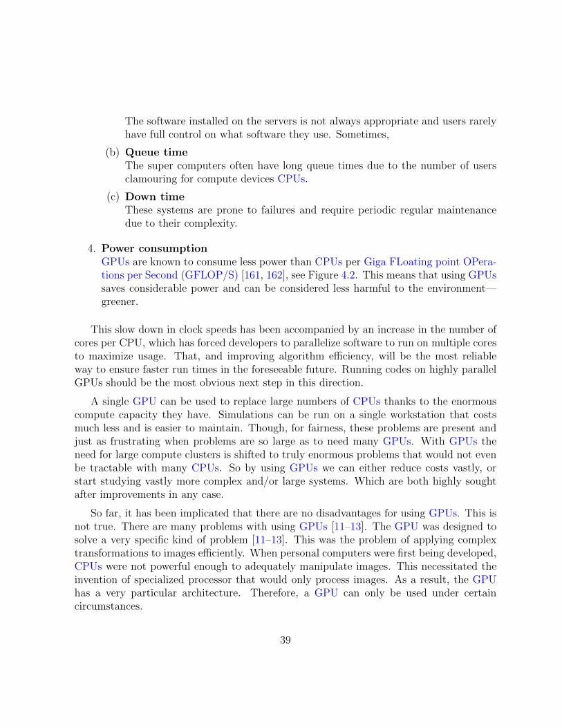
The software installed on the servers is not always appropriate and users rarelyhave full control on what software they use. Sometimes,

(b) Queue timeThe super computers often have long queue times due to the number of usersclamouring for compute devices CPUs.

(c) Down timeThese systems are prone to failures and require periodic regular maintenancedue to their complexity.

4. Power consumptionGPUs are known to consume less power than CPUs per Giga FLoating point OPera-tions per Second (GFLOP/S) [161, 162], see Figure 4.2. This means that using GPUssaves considerable power and can be considered less harmful to the environment—greener.

This slow down in clock speeds has been accompanied by an increase in the number ofcores per CPU, which has forced developers to parallelize software to run on multiple coresto maximize usage. That, and improving algorithm efficiency, will be the most reliableway to ensure faster run times in the foreseeable future. Running codes on highly parallelGPUs should be the most obvious next step in this direction.

A single GPU can be used to replace large numbers of CPUs thanks to the enormouscompute capacity they have. Simulations can be run on a single workstation that costsmuch less and is easier to maintain. Though, for fairness, these problems are present andjust as frustrating when problems are so large as to need many GPUs. With GPUs theneed for large compute clusters is shifted to truly enormous problems that would not evenbe tractable with many CPUs. So by using GPUs we can either reduce costs vastly, orstart studying vastly more complex and/or large systems. Which are both highly soughtafter improvements in any case.

So far, it has been implicated that there are no disadvantages for using GPUs. This isnot true. There are many problems with using GPUs [11–13]. The GPU was designed tosolve a very specific kind of problem [11–13]. This was the problem of applying complextransformations to images efficiently. When personal computers were first being developed,CPUs were not powerful enough to adequately manipulate images. This necessitated theinvention of specialized processor that would only process images. As a result, the GPUhas a very particular architecture. Therefore, a GPU can only be used under certaincircumstances.

39

Issues with using GPUs:

1. Dependence on CPUsGPUs cannot be used as general purpose processors due to the highly specialized

nature of GPU hardware design. Consequently any programs that utilize GPUs mustbe managed by a CPU, see figure 4.7. This may change in the near future with pro-cessors that borrow architectural principles from both CPUs, named HeterogeneousSystems Architecture (HSA). However, even with HSA devices, complexities will stillexist and glsgpu acceleration techniques will still be needed for them.

2. ComplexityThe highly parallelized hardware architecture of GPUs exposes programs to highlyesoteric constraints on algorithm design and validation. It is very likely that seem-ingly simple algorithms would have to be heavily redisigned to maximize performancegains. If code algorithms are not written correctly, then using GPUs may actuallyyield worse performance than CPUs due to the slower clock frequencies of GPUs.

3. InterfacingTargeting the GPU for executing simulation code is non-trivial. Until fairly recently,this was not even possible as there were no Application Program Interfaces (APIs)available to do floating point math normally. So all physical problems had to be recastinto graphics processing problems which was quite non-intuitive. This problem hasbeen solved somewhat with the introduction of some libraries such as The ComputeUnified Device Architecture (CUDA) and Open Compute Language (OpenCL). Theselibraries have made interfacing with GPUs simpler.

4. Problem dependenceThe specialized nature of GPU architecture makes the device only good at solvingcertain types of problems [11, 13]. Some criteria for choosing problems to accelerateon GPUs are:

(a) Large computational requirementsThe GPU only outperforms the CPU when its hardware is being used to the

fullest. Small calculations will generally be more efficiently computed on theCPU

(b) Substantial parallelismIt follows from issue 4a that the calculation must be parallelizable. Problemswith a lot of recursion most probably will not benefit form GPU acceleration (e.g.

40

computing the Fibonacci sequence or the factorial of a number). FortunatelyMD can be parallelized efficiently.

(c) Latency independenceThe calculation being done is not affected by latency. Because of issues 1 and 3,there is a large overhead in transferring data to and from the GPU. This is reallyonly a problem for graphics applications and is included here for completeness.It does not affect MD code very much as, typically, initial conditions have tobe moved to the GPU only once. Data is read from the GPU only to output it.There are also ways of hiding this latency when running calculations, but thatis out of the scope of this thesis.

Until a few years ago, direct floating point math was not possible on GPUs. Theeffort to use GPUs for general computations is called General Purpose GPU (GPGPU) [12]computing. GPGPU has become significantly easier with the advent of new hardware whichsupports floating point arithmetic (needed for scientific computing), and new softwarelibraries and standards that make interfacing with GPUs more efficient are simple. Softwaresuch as OpenCL and CUDA.

With all of the problems with CPUs and GPUs in mind, there still are certain problemsparticularly well suited to execution on GPUs[11, 13, 65, 163, 164]. It has been shown thatMD simulations are definitely well suited to GPU acceleration[11, 65, 165–170], they havelarge computational requirements, benefit from parallelism, and can be independent oflatency. When applied correctly, GPUs will always outperform CPUs by at least 2–3times, and in some cases by a few orders of magnitude. See figure 4.2 for some comparisonof performance information.

Stone et al. made a simple comparison, shown in table 4.1. Some energy evaluationkernels were written in c and in CUDA with varying levels of optimization. C code wascompiled with the Gnu Compiler Collection (GCC) and the Intel C Compiler (ICC), ICCis known to yield higher performance binaries, especially on Intel devices. A large portionof the speed up on GPUs can be attributed to the significantly faster memory accessspeeds on GPUs thanks to the highly optimized hardware design and faster GPU memoryclocks. Anderson et al. [65] found that many aspects of MD, including Lennard-Jones forcecalculation, neighbour list generation, can be sped up significantly on GPUs [65].

41

Figure 4.2: Comparison of performance data of some high end processors. AMD CPUs arenot included as the trends are largely the same. AMD APUs are not included because theycannot be directly compared to GPUs and CPUs. (a) The number of processing elementsper processor; GPUs have considerably mode processing elements than most CPUs. (b)The theoretical peak performance of each processor; GPUs outperform CPUs easily. (c)The performance of the processing elementsCPUs in general have higher performing cores,but GPUs have many more. Enough to outperform CPUs. GPUs have many more cores. (d)Inspite of their higher performance, GPUs are the more energy efficient alternative. Creditto Mark Rupp[162], CC license.

With all of this in mind, it may be concluded that an efficient solution for MD shouldcontain parts that use both CPUs and GPUs. The goal of the work in this thesis is toproduce such a program that can simulate cellular behaviour with a model based on MDprinciples, and accelerate the appropriate parts (force calculations, velocity and position

42

Table 4.1: Direct Coulomb summation performance comparison. Performance was com-pared on the CPU with compiled with GCC and ICC and on the GPU with code compiledwith CUDA at different levels of optimization. Clearly, GPUs are superior for energy eval-uations even with minimal optimization. Data taken from Stone et al. [11].

Kernel Performance Normalized to IntelC

BillionEvaluations/sec

GFLOPS

CPU-GCC-SSE 0.052 0.046 0.28CPU-ICC-SSE 1 0.89 5.3CUDA-Simple 16.6 14.8 178CUDA-Unroll8x 38.9 34.6 268CUDA-Unroll8y 40.9 36.4 191CUDA-Unroll8clx

44.4 39.5 291

updates) on GPUs. This code, in conjunction with the force-field described in Chapter 5,will be used to model cell behaviour.

If following sections GPU architecture and programming will be introduced. The termsused will be CUDA terms for the sake of simplicity, but the concepts are common betweenCUDA and most other libraries. The remainder of this chapter may seem like it onlyapplies to GPUs but much of it will be a general introduction to programming on anyparallel device. Thanks to libraries like OpenCL (which was not used for the program usedin this thesis), the principles will remain the same regardless of device.

4.2 GPU Architecture

In this section a brief overview of GPU architecture will be given. A detailed analysis ofthe design specifications is out of the scope of this thesis as it differs from GPU to GPUdepending on brand and model type. A cursory understanding of GPU design should besufficient to proceed. Readers looking for more detailed descriptions are referred to [12,13].

Simply speaking, the entire goal with GPU hardware design is to supply a greaternumber of computing cores to do the calculations. Until recently, GPU hardware wasonly suitable for image transformations. Newer GPUs are capable of doing floating pointmath at rates much faster than CPUs. Figure 4.3 shows the complexity of some NVIDIAGPUs, other types of GPUs are not much different conceptually. There are many levels

43

of hierarchy and caching that make the design complicated. A simpler depiction of CPUsand GPUs is presented in Figure 4.4.

Figure 4.3: Core placement and categorization on two kinds of NVIDIA GPUs. (a) TypicalFermiTM NVIDIA GPU design, the cores are placed within Stream Multiprocessors (SMs)which are themselves inside placed into Graphics Processor Clusters. There are multiplelevels of memory (caches) but the most relevant to GPU developers is the DRAM memory.(b) This picture shows a more detailed representation of a KeplerTM type gpu. Thereare multiple control circuits including circuits that manage the memory accessing and thecaching of data in the different levels of cache.

The designs shown in Figures 4.3 and 4.3 are far too complicated to considered exactlywhen coding, especially when targeting more than one kind of GPU. The structure of theGPU is abstracted into a more tractable form. For the sake of generality, some generalterms are defined here. Newer CPUs are being designed with many cores incorporated intothem, so it is beneficial to use some common terms that are equally applicable to multicoreCPUs, GPUs, and any other parallelized computational devices. The managing device willbe named the “Host” and the computational device the “Device”. A host may have anynumber of devices. A PC may contain one host (the main CPU), and one or more GPUsdevices. A large compute server may contain hundreds or thousands of devices. For theremainder of this section, device and GPU are used interchangeably.

As shown in Figure 4.5, each device can be divided into a collections of Compute Units(CU), the compute units access global memory (G) as a group simultaneously. Thesecompute units are nothing but a collection of Processing Elements (PE) (cores) with com-mon Local Storage (LS), each processing element contains within another cache of private

44

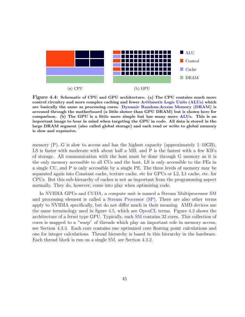
Figure 4.4: Schematic of CPU and GPU architecture. (a) The CPU contains much morecontrol circuitry and more complex caching and fewer Arithmetic Logic Units (ALUs) whichare basically the same as processing cores. Dynamic Random-Access Memory (DRAM) isaccessed through the motherboard (a little slower than GPU DRAM) but is shown here forcomparison. (b) The GPU is a little more simple but has many more ALUs. This is animportant image to bear in mind when targeting the GPU in code. All data is stored in thelarge DRAM segment (also called global storage) and each read or write to global memoryis slow and expensive.

memory (P). G is slow to access and has the highest capacity (approximately 1–10GB),LS is faster with moderate with about half a MB, and P is the fastest with a few KB’sof storage. All communication with the host must be done through G memory as it isthe only memory accessible to all CUs and the host, LS is only accessible to the PEs ina single CU, and P is only accessible by a single PE. The three levels of memory may beseparated again into Constant cache, texture cache, etc for GPUs or L2, L1 cache, etc. forCPUs. But this sub-hierarchy of caches is not as important from the programming aspectnormally. They do, however, come into play when optimizing code.

In NVIDIA GPUs and CUDA, a compute unit is named a Stream Multiprocessor SMand processing element is called a Stream Processor (SP). There are also other termsapply to NVIDIA specifically, but do not differ much in their meaning. AMD devices usethe same terminology used in figure 4.5, which are OpenCL terms. Figure 4.3 shows thearchitecture of a fermi type GPU. Typically, each SM contains 32 cores. This collection ofcores is mapped to a “warp” of threads which play an important role in memory access,see Section 4.3.3. Each core contains one optimized core floating point calculations andone for integer calculations. Thread hierarchy is based in this hierarchy in the hardware.Each thread block is run on a single SM, see Section 4.3.2.

45

Global Memory

PE

LS

P

Global Memory

Constant Memory

Figure 4.5: From the programmers perspective, any parallel device can be approximatedwith this structure. Note that the number of elements shown here is just an example, actualdevices can have any number of CUs and PEs.

4.3 Programming Perspective

The hardware abstractions being out of the way, the programming perspective will beillustrated in this section. The GPU architecture is important when aiming for the highestperforming code. In table 4.1, Stone et al. [11] showed that GPU code without optimizationis still very fast. So, when coding, at least initially, a detailed picture of hardware is notneeded as much as when optimizing. From the programmers perspective, the GPU is notmuch different from a CPU with a very large number of cores.

A unit of computational work is named a kernel [171]. Kernels contain a module ofcode that does a certain task. It can be thought of as a function or subroutine that runson the compute device (GPU). Listing 1 shows some sample code with the same kernelimplemented in C and in CUDA. The kernel can be executed in a serial manner on theCPU or in parallel on the GPU.

CUDA code follows the same standards of C/C++ with some some extensions anddifferences. The differences from C/C++ include things like lack of recursion [171, 172],no Object Oriented Programming (OOP). CUDA also introduces some new data typesand built-in functions to ease programming. There are also some libraries that make

46

programming with CUDA almost indistinguishable from programming in C++ such asThrust [173] and boost.compute (still in testing, kylelutz.github.io/compute/). Someaccelerated versions of standard libraries: cuFFT, cuBLAS, CUDA Math Library, etc.There is no need to use C/C++, CUDA supports Python, FORTRAN, C#, and Java.

As an example, consider the task of adding two vectors, c = a+b. CPU code is straightforward. This task can be done with a for loop sequentially. Since elements of a and b canbe summed independently, the operation can be parallelized to execute on multiple coreson the GPU, see figure 4.6. Assuming the CPU and GPU cores have the same clock, theoperation can be sped up by eight times.

Parallel GPU Execution

Serial CPU Execution

Figure 4.6: Diagram showing single threaded CPU execution and multithreaded GPUexecution. Note that the segments representing a, b, and c reside on either host DRAM ordevice DRAM depending on what device executes them. From the programming perspective(refer to Section 4.3.2), the CPU has one 1D block of one thread and the GPU has one 1Dblock of 8 parallel threads.

Listing 1 shows CPU C code and GPU CUDA code. CUDA syntax is not very differentfrom regular C syntax. The variable m specifies the block size which is the number of con-current threads. If the size of a, b, and c is greater than the number of maximum possibleconcurrent threads GPU_MAX_THREADS, then m = n/GPU_MAX_THREADS and the calculationis looped m times, n threads running at a time. At first glance, this might seem to be quitea fatal limitation. A very large number of threads can be running on modern GPUs, about

47

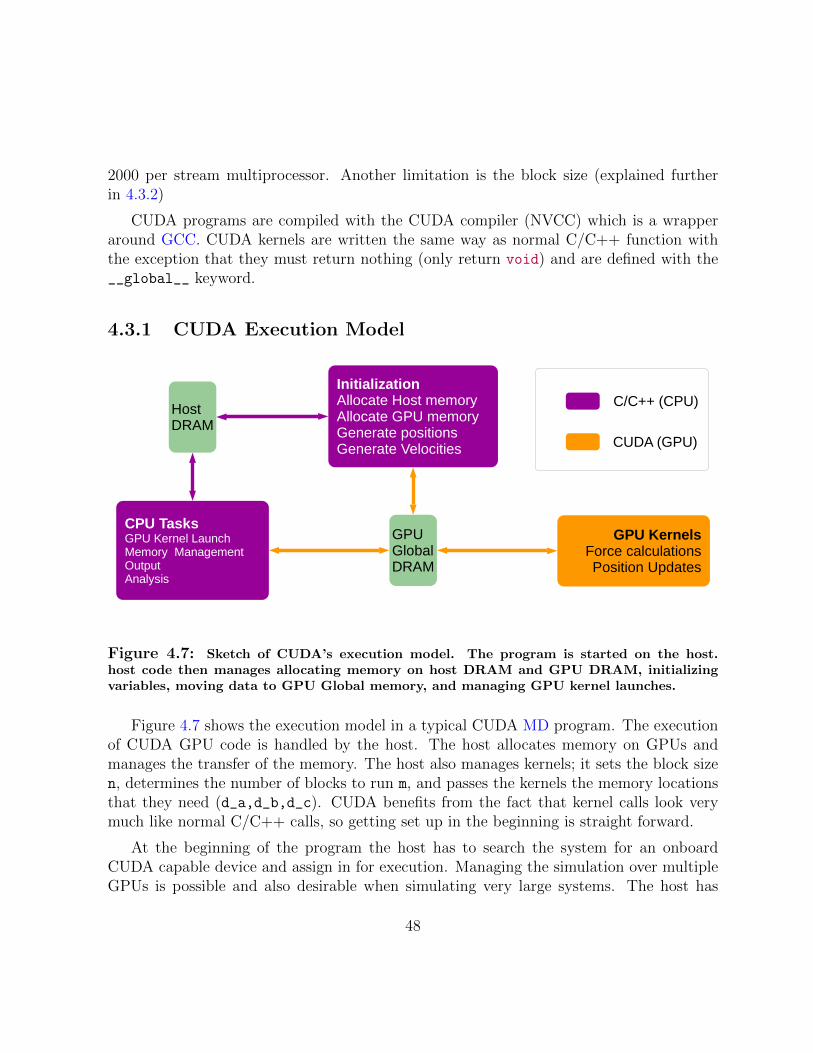
2000 per stream multiprocessor. Another limitation is the block size (explained furtherin 4.3.2)

CUDA programs are compiled with the CUDA compiler (NVCC) which is a wrapperaround GCC. CUDA kernels are written the same way as normal C/C++ function withthe exception that they must return nothing (only return void) and are defined with the__global__ keyword.

4.3.1 CUDA Execution Model

InitializationAllocate Host memoryAllocate GPU memoryGenerate positionsGenerate Velocities

CPU TasksGPU Kernel LaunchMemory ManagementOutputAnalysis

GPUGlobalDRAM

HostDRAM

GPU KernelsForce calculationsPosition Updates

C/C++ (CPU)

CUDA (GPU)

Figure 4.7: Sketch of CUDA’s execution model. The program is started on the host.host code then manages allocating memory on host DRAM and GPU DRAM, initializingvariables, moving data to GPU Global memory, and managing GPU kernel launches.

Figure 4.7 shows the execution model in a typical CUDA MD program. The executionof CUDA GPU code is handled by the host. The host allocates memory on GPUs andmanages the transfer of the memory. The host also manages kernels; it sets the block sizen, determines the number of blocks to run m, and passes the kernels the memory locationsthat they need (d_a,d_b,d_c). CUDA benefits from the fact that kernel calls look verymuch like normal C/C++ calls, so getting set up in the beginning is straight forward.

At the beginning of the program the host has to search the system for an onboardCUDA capable device and assign in for execution. Managing the simulation over multipleGPUs is possible and also desirable when simulating very large systems. The host has

48

to manage the distribution of the work across the GPUs. GPUs can be thought of ascalculation machines that must be managed manually.

All data is communicated to the GPU through the GPU’s on board of global memory.Regardless of platform, moving data from one region of memory to another region isvery time consuming, especially if the memory is in different locations. Memory transfermust be minimized in order to maximize performance because there is a highly latency incommunication with GPUs. Thankfully, the communication line with GPUs has a fairlylarge bandwidth, 100’s of GBs/sec., so a lot of data can be moved at once. Once data hasmoved to the GPU, it should be kept there until it absolutely must be sent back to thehost. Minimizing the need for data manipulation on the host entirely should always be oneof the goals of any good algorithm. Thanks to this execution model, the idle CPU timecan be used to perform other tasks

Once on the GPU, the simulation can begin in earnest. Ideally, all of the resources ofthe GPU are being used at maximum capacity and all the host is doing is waiting for theGPU to finish. However, because there is no way for the GPU to access storage drives,or manage memory, the data has to be transferred back to the host every once in a whilefor output. In the case of the cell division code, data has to be moved to handle the celldivision part.

At the end of the simulation, since the host manages GPU memory, it has to handlereleasing no longer needed resources. Though, if the program is to end at this point, CUDAis intelligent enough to release that memory when the program ends. Nevertheless, it isgood practise to keep careful track of memory because chasing memory leaks on the GPUcan be quite frustrating.

4.3.2 Thread Hierarchy

A kernel is a task that applies to large amounts of data. With each kernel, a single blockof instructions (a single function) is being applied to a large amount of data. This wayof data processing is named Single Instruction Multiple Data (SIMD) in computer scienceand is the most obvious target for parallel computing. A thread is the concept of a kernelbeing executed once on some piece of data once. In other words, each kernel is executedas a, potentially large, collection of threads on large amounts of data. Now, the focus isshifted to thread management from the programmer’s perspective. It is useful to know theworkings of the hardware for optimization, but the hardware complexity is abstracted outin the CUDA and OpenCL API. So, at least in the beginning of a project, it is useful to

49

focus on the basics of GPU programming. Readers interested in more detail are referredto [172]

The size of data that is needed for MD is very large, the position and velocity of,and the force on each atom in a system should be calculated simultaneously. If we takethese tasks as one function, then this function is of one (discrete) variable, namely theindex of each atom in some master data array containing the coordinates of all atoms.In this sense, this is a ‘one dimensional’ problem (see Figure 4.7). One can imagine suchproblems with higher dimensionality. There are many problems in science and engineeringthat are applied over 2D or 3D grids, for example, the temperature distribution on a metalplate. For conceptual compatibility and ease of programming, it is convenient to bundleconcurrent threads in 1D, 2D, 3D, or N-dimensions.

This is recognized in the field of GPU acceleration, and the API is designed with thisfunctionality. OpenCL kernels can be bundled in N dimensions, whereas CUDA is limitedto three. Keep in mind that this dimensional bundling does not limit the problems thatcan be solved at all, one may choose to implement everything in one dimensional blocks ifthat is desirable. This bundling is only for convenience.

Figure 4.8: Here is a two dimensional set up of thread blocks is shown. In this figure,following the convention in Eq. 4.1, t1 = 6, t2 = 4, t3 = 1 and b1 = b2 = 2, b3 = 1. So that thethread index of the thread circled red is thread (4, 1, 0) in block (1, 0, 0). That thread alsohas a global index of (10, 1, 0).

50

In CUDA terms, all threads are bundled into blocks. In each block, threads can beindexed by a one-dimensional, two-dimensional, or three-dimensional index. Similarly, theblocks can be indexed by one-dimensional, two-dimensional, or three-dimensional index.The total number of threads launched by the host is given by

nt = t1t2t3 · · · tn · b1b2b3 · · · bm (4.1)

where t is the number of threads in along dimensions 1, 2, 3, and b is the number theblocks. Of course with CUDA, n ≤ 3,m ≤ 3. Depending on the hardware, there can beconstraints on nt and other strategies will be needed to solve that problem (multiple GPUsor looping over the work with a single GPU). In new CUDA GPUs, tmax = t1t2t3 = 1024,so nt,max = 1024bmax. bmax depends on the hardware and implementation, it is difficultto determine a priori as it depends on the number of registers available per thread. bmaxplays an important role in optimizing occupancy. Once again, this is just a limit on howmany threads and blocks can be launched at a single time. If more are needed, then thecalculation can be looped or split among GPUs.

device occupancy is defined as the ratio of the number of active threads per devicedivided and the maximum possible number of threads per device. Obviously, this shouldbe kept as close to one as possible. The GPU hardware and drivers are designed to do thisas much as possible. Maximizing device occupancy is difficult, detailed knowledge of GPUdesign, API, and thread hierarchy are required. Occupancy is affected by choice of blocksize, shared memory usage, private memory usage, and hardware limitations.

At first glance this splitting of threads into blocks may seem arbitrary, it actually servestwo vital purposes [172]: (1) This indexing gives a precise identity to each thread and thisidentity can be accessed within a kernel, (2) block and thread breakdown informs memorybreakdown and vice-versa. Each thread has private memory to itself, all of the threads haveaccess to shared memory in a block, and all blocks have shared access to global memory.Figure 4.8 shows an example of two dimensional thread blocks. Tuples of indices are usedto identify threads, they can have a local index which requires indexing blocks and threads,or global indices. It is necessary to calculate the global index because data spans all ofthreads. The CUDA code snippet below shows sample code with this indexing in action.Assume that there are three arrays, one for each of the Cartesian axes, that contain theposition of all atoms. The positions of can be distinctly accessed with a unique index i.With this information, we launch the kernel KernelExample once for each atom. So theindex of the thread can be converted to the index of corresponding atom.

__global__ KernelExample (float* Xdata, float* Ydata, float* Zdata){

printf("BlockID = (\%d, \%d, \%d), ThreadID = (\%d, \%d, \%d)\n",

51

blockIdx.x, blockIdx.y, blockIdx.z,

threadIdx.x, threadIdx.y, threadIdx.z);

// Below since Ydata spans all thread blocks, we get the global

// address of a thread by multiplying by blockDim.y

int i = blockIdx.y*blockDim.y + threadIdx.y;

float y = Ydata[i];

}

Special reserved variables such as threadIdx store the index of each thread. Thesevariables are used to access data in global memory, or in shared memory among threadsin the same block.

4.3.3 Memory Hierarchy and Access

The placing of threads in separate blocks brings control to memory access and is an impor-tant factor in optimizing performance. All threads always have access to global memory.There is also shared memory that is made available to all threads of the same block. Ablock of threads will only every run on a single Stream Multiprocessor (PE in Figure 4.5).And then, each thread has private memory to itself. Private is the fastest to access, shareda little slower, and global memory is the slowest to access [12, 172]. Shared memory andprivate memory is temporary and has the same lifetime as its block or thread respectively,global memory persists over many kernel calls, as long as the host does not release it.

Not only is global memory slow to access, but access to global memory has to be donein certain ways to maximize speed. Memory access occurs 16 threads at a time regardlessof how many threads are requested to access memory [172]. 32 threads are named a warpin CUDA terminology, so memory access occurs in half-warps. This means block sizes mustbe multiples of 2, as required by CUDA, and also multiples of 16 to maximize memoryaccess efficiency. OpenCL does not require even block sizes [174], but still benefits greatlyby making block sizes a multiple of 16 on NVIDIA devices.

__global__ void MemoryAccessKernel(float* array){

int index = blockIdx.x * blockDim.x + threadIDx.x;

float element = array[index];

}

MemoryAccessKernel<<<1, 1>>> (float* arrayWithOneElement);

MemoryAccessKernel<<<1, 16>> (float* arrayWith16Elements);

MemoryAccessKernel<<<1, 17>> (float* arrayWith31Elements);

52

The first two kernels will take the same amount of time to complete, while the lastkernel call will take double the time of the first two kernels even though it is accessingalmost the same number of memory locations as the second kernel call. Memory accesslatency is very often a major bottleneck in kernel execution. The following section containssome strategies that can be used to maximize memory access performance, and maximizeperformance in general. Following these strategies is beneficial, but should not be a priorityuntil after the software is shown to be correct and without any bugs.

4.3.4 Some strategies to enhance GPU performance

Generally speaking, kernels can be divided into three types: latency bound, computebound, and memory bound.

(1) Optimizing latency bound kernelsLatency bound kernels depend on their execution by the host. They are optimized byadjusting the execution parameters that were set by host code. Latency problems canoccur when not threads are not broken down into blocks optimally.

(a) Maximize occupancyThe GPU has built-in circuitry that launches units of work on each SM, if thework given is not enough to saturate this process, then performance is wasted/lost.This requirement is difficult to meet and should be left to the end of the project.Maximizing occupancy helps greatly to shifting the slowest step to memory access.

(i) Saturate the GPUAdjust block size, private memory, and shared memory usage such that thereis always an abundance of work to be done by the hardware.

(ii) Concurrent kernel executionThe host normally waits until after the kernel has finished executing to re-sume. If adjusting the launch parameters does not help, many kernels canbe launched concurrently.

(2) Optimizing compute bound kernelsCompute bound kernels are kernels that spend most of their time doing calculations,this type of kernel can be optimized with algorithmic improvements. Sometimes, simplechanges in the way calculations are carried out can result in significant performancegains.

53

(a) Uniform execution pathThe GPU executes instructions uniformly for an entire warp. In order to maximizeusage, all threads should have the same execution path (run the same code). Thisproblem only occurs if the divergence is among threads of the same warp (sameblock).

(i) Avoid thread branchingSome tasks require divergence depending on the data being processed. Inthose cases, it may be beneficial to decide what data needs to be processedon the host, and launch kernels that work with only that data. The codesnippet below shows a bad example of thread branching—the first 6 threadsare idle with this execution path.

if (threadIdx.x > 5)

DoSomething();

else

DoNothing();

(b) Loop unrollingThere is a performance benefit to type out each iteration of for loop. Thisincreases the amount of work done for each thread so efficiency is improved sig-nificantly.

(c) Intrinsic/Fast MathIf exact matching with CPU is not required, then there are intrinsic optimizedversions of common math functions that should can be used for performance.For example, __sinf() vs. sinf(). Readers are referred to CUDA/OpenCLdocumentation [174, 175] for more details regarding intrinsic functions.

(3) Optimizing memory accessMemory bound kernels are kernels that spend time accessing memory. These kernelscan optimized by correctly requesting memory reads (or writes).

(a) Coalesced memory accessAs noted before, memory access is done on a per warp, in some cases per half-warpdepending on GPU, basis. Furthermore, there is a minimum transaction size foreach memory read. On Kepler GPUs it is four warps (128 threads) [176], sincememory transactions are always done n warps at a time, it is good practise toassume minimum transaction of 32 threads. Additionally, It is always preferableto access contiguous blocks of memory at a time. That means that threads in asingle warp should be accessing adjacent regions of memory always. If this is doneproperly, memory access can be “coalesced” into a single operation.

54

(i) Align memory access in a blockThread index should be aligned with element index to maximize performance.For example, thread 0 accesses element 0, thread 1 accesses element 1, etc.Threads can also be aligned with an offset, which should be a multiple ofminimum transaction size (32 bytes). Thread 0 accesses element 8, etc.

// example of aligned memory reads

float a = bigArray[threadIdx.x];

// with an offset

float b = bigArray[threadIdx.x + 8];

Below is an example of inefficient access. Every third element is being ac-cessed.

float a = bigArray[threadIdx.x*3];

Finally, we have an example of misalignment, this occurs when the offset isnot a multiple of the minimum transaction size of memory.

float a = bigArray[threadIdx.x+13];

(ii) Avoid broadcastingBroadcasting is the access of multiple threads to the same, memory location.Instead constant memory should be used. Not only is many threads read-ing from the same memory location inefficient but writing to it can lead todifficult to debug race conditions.

(iii) Avoid concurrent thread writesThe opposite of broadcasting is when multiple concurrent threads (i.e. threadsin the same block) attempt to update a single memory location. This leadsto undefined behaviour and is named a race condition. Race conditions donot necessarily lead to lower performance but can lead to incorrect resultsand complicated bugs.

55

1 /****** CPU code segment start ********/

2 void add (float* h_a, float* h_b, float* h_c, int n){

3 for (int i = 0; i < n; i++){

4 h_c[i] = h_a[i] + h_b[i];

5 }

6 }

7 add(h_a, h_b, h_c, n);

8 output(h_c);

9 /******** CPU code segment end ********/

10

11 /****** GPU code segment start ********/

12 __global__ void add(float* d_a, float* d_b, float* d_c){

13 i = blockIdx.x*blockDim.x + threadIdx.x;

14 /* blockIdx.x iterates from 0 to m-1

15 blockDim.x equals n

16 threadIdx.x iterates from 0 to n-1

17 */

18 d_c[i] = d_a[i] + d_b[i];

19 }

20 HostToGpuCopy(h_a, d_a);

21 HostToGpuCopy(h_b, d_b);

22 add<<<m, n>>>(a, b, c);

23 /* m = 1 if n <= Max number of threads (can be 512 or 1024)*/

24 GpuToHostCopy(d_c, h_c);

25 output(h_c);

26 /******** GPU code segment end ********/

Listing 1: Adding two vectors is not very different when comparing GPU and CPU code.The number of threads to launch is specified by host code and device code contains specialvariables with the thread index information.

56

Chapter 5

Methods and Implementation

As described earlier, modelling cell behaviour could be highly challenging due to highlycomplex nature of most cells. An average cell contains many multitudes of differentmolecules, large and small, that all come with their own particular complex behavioursand interactions. These complex interactions are, of course, all highly interesting on theirown, but they unfortunately make studying the cell as a whole an intractable problem.

Fortunately, cell-cell interactions can be approximated through a variety of approxima-tions, see Chapter 3. However, these approximations tend to be ad hoc in the sense thatthey can only model limited behaviours of cells in certain regimes.

We will approach building this model from two angles. The first being the theoreticalbasis, physics and mathematics, for the model. And, naturally, the second will be actualimplementation in C++. C++ was chosen for out simulation because of the variety oftools and libraries available for acceleration. We will be using CUDA for our accelerationneeds.

The cells are modelled with Molecular Dynamics techniques, where each cell is com-prised of a spherical membrane made of a fixed, though optionally can be varied, numberof particles in a force field. The force field itself contains terms for the surface tension ofthe cell membrane, the adhesion (or friction) between cells, the repulsion between cells,and a term for the drag that the cell experiences in its medium. This model is based onwork by Mkrtchyan et al [15] in 2014, and Astrom and Karttunen [14] in 2006.

The simulation is then optimized to run on GPUs. The optimization method will beoutlined in some detail and some strategies that can be employed to further optimized thiscode will be discussed.

57

In Section 5.1, the model will be defined and described in detail. Section 5.2 describesthe values that are given to the parameters that are part of the model, and Section 5.4describes the implementation with CUDA and the design choices that were made to increaseperformance.

5.1 The Force-Field

First we will define the force-field of the particles in our simulation. There are two broadcategories within the force-field that have to be defined. That is done in the followingsections.

In Section 5.1.1, the assumptions that are made with this simulation method are de-scribed and justified. It is important to begin with a relatively simple model to begin, thenmore complexity and detail can be added if needed.

In Section 5.1.2, the structure of the model cell will described in detail, this includes thegeometry of the particles that make up the cell and the physics of the cell membrane. Tosummarize, each cell is modelled using the C180 molecule [177–179] as a template, wherethe particles and bonds are treated as balls and springs.

Section 5.1.3, the interactions that govern the interactions between the particles withina cell are described. The forces defined here govern the integrity of the cell body andregulate its growth.

In Section 5.1.4, the methods used to model inter-cellular interactions will be described.These include the final elements of the MD force-field. We will see that interactions betweencells is broken down into an adhesive force and a repulsive force. Another force is adissipative one that is used to model the environment around the cells.

5.1.1 Assumptions in the Model

The ultimate goal of this work is to simulate the behaviour of cells as completely aspossible. However, we first begin with a simpler model then, more complexity and detailcan be added if needed. Hence, some assumptions are made to simplify the constructionof the model.

1. There is only one cell type.All of the cells in the system will be identical in structure. They will be allowed tobehave independently. Some of the remaining assumptions follow from this one.

58

2. All cells grow at the same rate.If able, all of the cells will grow and the same rate. To be more clear, the driving

force behind cell growth, discussed in section 5.1.3, will be the same for all cells.Cells also grow at the same rate whatever their surface areas.

3. External conditions do not affect the simulation.External conditions such as pressure, temperature, humidity are ignored. These canbe indirectly modelled by setting the parameters discussed in sections 5.1.3 and 5.1.4,and therefore can be easily introduced into the model at a later time. Anotherconsequence of this assumption is that the availability of nutrients in the system,and the cells’ access to those nutrients, are both ignored. However, these can beincluded back into the model.

4. Cell death is ignored.In reality, cells die either because they have depleted their lifetime, due to un-favourable conditions, or both [180, 181]. However, this fact is ignored. Thoughit is possible to add cell death to the model, it will not be explored in this thesis.

5. The cells exist in an infinite space.The cells will not be confined spatially, at least initially, in anyway. This not onlymeans that the cells will not be hindered in any way, but also means that there areno periodic boundaries or any other boundaries of any time.

6. All of the cells are spherical in their natural state.This comes from the fact that animal cells favour a rounded structure due to theircortex contractility[35, 36].

7. Cell-cell interactions are isotropicCells can interact differently depending on direction. But this is ignored for ourmodel, the cells in our simulations interact uniformly with each other.

8. Hertwig’s rule can be ignored.The cell division plane will always be random and through the centre of mass, see 5.3.

9. Each daughter cell will be identical.The model will not, initially, do any asymmetric cell division, see 5.3.

59

5.1.2 The Model Cell

The cell itself will be modelled as sphere made up of a number of particles with uniformmass. The mass of the particle in itself is an interesting parameter and will be discussedin more detail in Section 5.2. Figure 5.1 is a sketch of how such models are constructed.

Figure 5.1: The ball and spring model. Figure shows a particle with an arbitrary numberof bonds. This particle has N springs connected to it.

We can easily calculate the forces on the particle as shown in equation (5.1). Basically,we do a vector sum of the force caused by each spring,

FS =∑i=1

Fi =∑i=1

−kixi, (5.1)

where xi denotes the displacement vector of the particle from the equilibrium positionof with respect to spring i. The spring force becomes an important element of the force fieldused in our Molecular Dynamics simulation. Given this very basic modelling technique,we can build particle model for the whole cell. However, we must first come with a generalmethod to represent the cell within our simulations.

A generalized spherical geometry is needed to build the cell itself. Coming up with

60

this geometry is not a trivial task. Because to be usable for the simulation, it must meetcertain criteria listed below.

Criteria for choosing the cell geometry:

Uniformity:The geometry should be more or less uniform. In other words, the distances betweenparticles should not change by very much over the surface of the sphere. This isto simplify the parametrization of the simulation in the future. Ideally, all of theparticle pairs will have the same bond length1

Simplicity:The geometry should be simple and well understood. The coordinates of the particlesthat make up our sphere should not be difficult to calculate. Ideally, an already knowngeometry should be used.

Versatility:The geometry should accommodate the physical changes that are expected with cellbehaviour. In other words, the geometry should allow for deformation and expansionwithout breaking down. Additionally, the geometry should be easily matched withbasic cellular structure. i.e. spherical cell should be modelled by a spherical geometry,ellipsoidal with ellipsoidal geometry, etc.

Spatial Resolution:The behaviours of cells can be highly complex as discussed in Section 2.1, so thereshould be enough points to accurately describe these behaviours. Conversely, whileit is true that a high resolution is needed, it must not be so high that it overwhelmsthe available computational resources.

Taking all of the above criteria into account, a simple model for the cell can be createdin 2D, however, this is not true for the 3D case. Mkrtchyan et al. showed a good sketch ofthe 2D model [15] which is reproduced in Figure 5.2. Figure 5.3 shows the 3D extensionto this model.

1 This way we can only worry about setting one bond length in our simulation. If in our geometry,there are many possible bond lengths for each bond, then they would each have to be set manually. Thisway we eliminate the degrees of freedom introduced by the geometry of the model cell. The effect of bondlength can be studied in greater detail at a later time.

61

(a) (b)

Figure 5.2: (a) The 2D model of the cell, all of the points are in the plane of the page,the various forces that act on each mass point are defined in Section 3.3 and [15]. (b) The3D model, the number of particles that make up the membrane is variable in theory, thoughit is 180 in all of the simulations run for this thesis. The cells tend to stay spherical unlessthey interact with surrounding cells or other surfaces in the system such as walls.

The 3D model itself is not much more complicated than the 2D model mathematicallyor conceptually, the complication arises from the numerical calculations associated withthe additional degrees of freedom introduced by modelling the system in 3D. Another noteis that each particle is bonded to three neighbours in the 3D model, one more than the 2Dcase.

The 3D geometry of the model cell may seem familiar, this is because the geometryis borrowed from the C180 fullerene [177–179]. The geometry of this fullerene is wellunderstood and fairly simple. One can quite easily find the coordinates of each atom froma variety of sources in the literature [36, 179, 182], another popular resource is M. Yoshida’slibrary of fullerene geometry [183]. The 180 particle mesh is also of sufficient resolutionto be able to model the cells, while keeping the load fairly low. A few thousand cellsamounting to less than one million MD particles can be modelled comfortably [65]. If ahigher resolution is needed, then this geometry can be changed to a larger fullerene. Theparticles are spaced more-or-less uniformly over the surface of the fullerene, so a uniformequilibrium bond length (equilibrium spring length) can be assumed. Lastly, the geometry

62

is approximately spherical, this is to ensure that we start from a simple model. Most cellstend to favour a spherical shape[35, 36], and different kinds of fullerenes exist that can beused to model different types of cells, though that is left for later research.

(a) (b)

(c)i

(c)ii

(c)iii

Figure 5.3: (a) The 3D geometry of the cell. (b) One isolated face of the cell, note thateach cell is bonded to three neighbours. (c) The different types of interactions that eachparticle experience in the force-field. There are spring forces (i), Attraction, repulsion, andfriction forces (ii), and a pressure force that governs the cell growth (iii).

Referring to Figure 5.3, we can now see a more detailed expression for the force on asingle particle in the cell shown in equation (5.2),

Fi =3∑j=1

FSij + +FP

i + FRi + FA

i + FFi , (5.2)

where FSij is the spring force associated with neighbouring particles within the same

cell, FPi is the pressure force acting of the membrane of the cell, FR

i is the repulsive forcebetween the membranes of different cells, FA

i is the adhesive force between membranesof different cells, FF contains the terms for friction between cells that hinders cellularrearrangements [15] FF,e and FF,m the friction with extracellular medium.

With the basics of the model in mind, we can proceed to define the force-field in more

63

detail. The force-field can be broken down into two basic categories. The interior of thecell and the exterior inter-cellular interactions.

5.1.3 The Cell Interior

There are two competing forces that act in the interior of the cell. The spring interactionbetween neighbouring particles, and the pressure force that will maintain the structureof the cell and also lead to the growth of the cell. The parameters shown below are indimensionless units, the basis for this scheme will be shown in Section 5.2.

The Spring Interaction force.

In reference to equation (5.2), we need to define the FS terms in the force-field. As alreadyshown in equation (5.1).

Figure 5.4: The unit vectors along each bond are shown. These are the vector terms usedto then calculate the spring for contribution.

Using the description of the bond2 vectors, we can represent the spring force explicitly.Now we need another index, j, to index the neighbouring particles.

Bij = ri − rj (5.3)

Rij = ‖Bij‖ (5.4)

2Note that this is not bonding between atoms in a molecule, it is just the attraction between points onthe mesh that forms the cell membrane. It comes from cortical actin filaments that give the cell its shape.

64

bij =Bij

Rij

(5.5)

FSij = E

A

Roij

bij(Rij −Roij) (5.6)

Where E is the Young’s Modulus of the spring and A its cross-sectional area, and in ourcase we set the cross-sections to be the same, so we can simply redefine ks = EA/Ro

ij and 5.6would be equally valid. The new kS variable is related to the cell cortex contractility,which depends on the structure of the cell membrane and will differ between different cells.Additionally, we can assume that the equillibrium bond length is the same for all particles.So we set Ro

ij = Ro, and

FSi =

3∑j=1

kSbij (Rij −Ro)− γintvij. (5.7)

The motion of the mass points in the spring interaction cannot be left to oscillate freelywhen interacting with each other. So an internal damping term, −γintvij, is introduced tomake sure that the mass points behave well where vij is the relative velocity of neighbouringmass points.

The Pressure Force

The internal pressure of the cell is the second element of the force-field that applies to thewithin the cells. The pressure force has is simpler by definition, the pressure is simply theratio between a force and the area it is applied to. In this case, the area that it is appliedis simply the surface area of the cell S. The internal pressure of each cell will apply auniform force on each particle in our membrane mesh. So the magnitude of the pressureforce on each particle will be equivalent. Cells are known to regulate their pressure beforemitosis [35, 37],

F Pi = PnSn, (5.8)

where n indexes each individual cell. However, referring to our assumptions (5.1.1), wesee that the cells will have the growth rate will be, independent of surface area. Hence our

65

pressure can be redefined as:Fi = PiS, (5.9)

where both Pi and S are constants. Thus we can regulate the growth rate by settingPiS. It is also possible to regulate the population of the system by developing a relationshipbetween PiS and the number of cells to study population dynamics in the future.

Figure 5.5: Diagram showing the normal vector to the surface of the cell pointing fromthe particle i. This normal vector gives us the direction of the pressure force.

From figure 5.5, we can then calculate the normal vector and use equation (5.9) for thepressure force on each particle as

ni ≈ (b1 − b3)× (b2 − b3) (5.10)

andFPi = PiSni (5.11)

This formulation follows the assumptions that we made in 5.1.1, assumption 2, onpage 59, states that the cell division shall not depend on the size of the cell. Therefore,PS is treated as its own variable that is not a function of cell radius rcell.

At any given pressure, the springs in that are used to model the cell cortex will extendor contract to attain an equilibrium volume. There is a threshold volume VD at which cellsdivide, with a corresponding pressure PDS. The growth rate of a cell can be thought ofas the rate at which the volume of the cell increases. That rate of volume increase is thenset by the rate of increase of internal pressure ∆(PS). ∆(PS) is set to be the same forall cells, PiS = PiS + ∆(PS) increases at a constant rate until VD is reached, then thePiS of each cell is optionally reset to a lower volume, and the process is repeated for eachdaughter cell.

66

5.1.4 Inter-cellular interactions

Cell-cell interaction is highly complex and varied [184–186]. Modelling such complex in-teractions is not a trivial task [14, 15, 62, 64]. Furthermore, the interaction type, strength,and directionality may vary greatly from cell to cell. However, we assumed that our cellswill interact isotropically with each other. This simplifies things for us greatly, as our cell-cell force-field need only depend on intercellular distance. We can completely generalizethe cell-cell interaction force into two parts, adhesion and repulsion. We have an additionalterm in the force-field for the viscous damping (or friction) force.

The attraction and repulsion forces are implemented as springs as well, with one dif-ference. They both will have a cut-off distance. This means that the springs only reactto compression or to extension, but not both. The repulsion and adhesion terms are bothcalculated for individual particles that are within repulsion and adhesion range of eachother.

The repulsion force is needed to prevent the cells from penetrating one another, andthe adhesion force is to simulate the interaction between different cells,

FRi =

∑j

FRij (5.12)

FRij =

{−kR

(RRc −Rij

)rij if Rij < RR

c

0 if Rij ≥ RRc

(5.13)

FAi =

∑j

FAij (5.14)

FAij =

{kA(RAc −Rij

)rij if Rij < RA

c

0 if Rij ≥ RAc

(5.15)

where j indexes the particles near the particle i but not part of the same cell as i. Herefour new parameters are introduced. RR

c and RAc are the repulsion and adhesion cuttoff

radii respectively. These have to be set manually in the simulation. Theoretically, thewould be related to the interaction ranges of different cells. And kA, kR are the springconstants that set the strength of the adhesive and repulsive forces. The constants kA, kR

can be related to the spring constant kS so that they can be set in comparison to the spring

67

force. kA = AkS and kR = RkS, where A and R are the adhesive strength and repulsivestrength, respectively.

The third term in the cell-cell interaction part of the force-field is the viscous damping.As cells move past each other, there should be friction between the two cell membranes.This friction would depend on the relative velocity of the cells. The relative velocity oftwo cells can reduced down to the relative velocity of particles in the membranes of thetwo cells vin,

vin = vi − vn (5.16)

FF,ei =

∑n

−γextvτin (5.17)

vτin = vij − (vij · n) n, (5.18)

where vτin is the tangential component of the relative velocity, γext is the damping themass points experience with points of other cells.

Finally, we have another friction. This force arises from the friction of the cells withtheir environment. Basically, there is some liquid, such as water perhaps, that hinders themotion of cells. The velocity of the particles is used to calculate this force,

FF,mi = −γmvi (5.19)

Thus, we have defined all of the terms in equation 5.2. Now we proceed to give valuesto all of the parameters (constants) that appear in the force-field.

5.2 Parametrization

The conceptual design of the simulation has been described in previous sections of thischapter. Now, the numerical values of the various constants are described. This is necessaryto be able to compare the results of simulations to experimental results.

The average volume of a human cell HeLa [187, 188] can be taken as Vavg ≈ 103 µm3 [189,190]. Using this, let’s take the unit of volume in the simulation to be [V]≈103 µm3. Con-sequently, [L]≈10 µm. Stewart et al. [35] measured the internal pressure of cells and found

68

that it was roughly 0.1nN µm−2, which can be rewritten as 10−8 N [L]−2. With, the unitvolume [V] given above we can approximate the total surface area of a cell with A≈5 [L]2.The outward force acting on each mass point is then given by F P≈5× 10−8 N. Each cellhas 200 mass points, so that the force on each mass point will be 1× 10−9 N. Thereforethe unit of force in the simulation will be set to [F]=10−9 N.

Stewart et al. [35] also estimated the Young’s modulus of mitotic cells and found themto be E ≈10−9 N µm−2 = 100 [F] [L]−2. E is related to ks with kS = Y Ao

Ro, where Ao is

the cross-sectional area of the cortex interconnects (thickness of the springs) and Ro is theequilibrium bond length. Ao approximated by Ao≈1 [L]2 assuming a diameter of 100 nm,and Ro with Ro≈0.1 [L] which is set by scaling the C180 structure to a volume of 1 [V].Then, the result is kS=1000 [F] [L]−1.

The adhesion and repulsion spring constants are defined by comparing their strengthto the spring forces. Mkrtchyan et al. [15] reasoned that the repulsion forces should bestronger than internal pressure forces. This follows form the fact that a pressure force of(PS)o is pushing outwards against neighbouring cells, so more rigid cells require strongerrepulsion between them. With this in mind R is set to (PS)o, so that the repulsion force isalways a factor of PS stronger than the spring force (kR = RkS); PS ≈ 100 as the internalpressure will be on the order of 100. With the same reasoning, the adhesion strength Ais set to 0.5 so that more rigid cells experience stronger adhesion, but still less than theattraction between points in the cell membranes (kA = AkS). These values will be variedand their effects studied later.

HeLa cells have a mass of 10−12 kg on average [191]. Given that the model cells haveabout 200 mass points, the unit of mass can be set to [M]≈10−13 kg by setting the mass ofeach cell to 10 [M]. Setting the mass of the cell to 10 [M] is done by arguing that the massof each mass point should be high enough to reduce motion as much as possible which isachieved by setting the mass of each mass point to M=0.05 [M], γm ≈ 10, γext ≈ 1.0, andγint ≈ 100. With this, the unit of time can be calculated with [T] =

√[M][Length]/[F] ≈

10−5s. Considering the fact the animal cells can take anywhere from an hour to a day[16],this unit is too small to set the time step in the simulation. Instead, the time step bymeasuring the number of time steps needed for a cell to divide, which is 1000 in thesimulation’s case. The time for a cell to go through one division is roughly T div = 1000∆t.∆t is set to 10−4 [T] for algorithmic reasons (stability and run time).

The growth rate of cells is set in the simulation with the parameter ∆(PS), which isnot going to be any one value. It will be varied to study what effects it has on the resultsfor simulations. The internal pressure of each cell will be regulated with ∆(PS) incrementsbetween a minimum and maximum pressure. The minimum pressure is set to (PS)o = 10

69

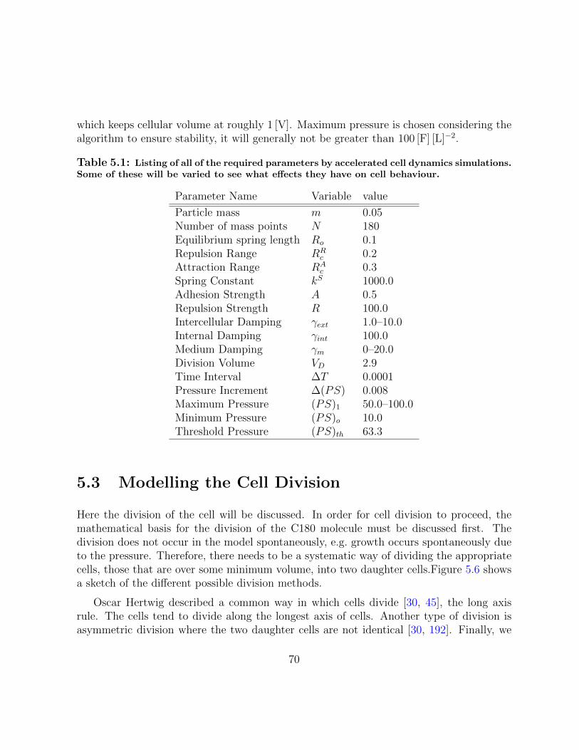
which keeps cellular volume at roughly 1 [V]. Maximum pressure is chosen considering thealgorithm to ensure stability, it will generally not be greater than 100 [F] [L]−2.

Table 5.1: Listing of all of the required parameters by accelerated cell dynamics simulations.Some of these will be varied to see what effects they have on cell behaviour.

Parameter Name Variable value

Particle mass m 0.05Number of mass points N 180Equilibrium spring length Ro 0.1Repulsion Range RR

c 0.2Attraction Range RA

c 0.3Spring Constant kS 1000.0Adhesion Strength A 0.5Repulsion Strength R 100.0Intercellular Damping γext 1.0–10.0Internal Damping γint 100.0Medium Damping γm 0–20.0Division Volume VD 2.9Time Interval ∆T 0.0001Pressure Increment ∆(PS) 0.008Maximum Pressure (PS)1 50.0–100.0Minimum Pressure (PS)o 10.0Threshold Pressure (PS)th 63.3

5.3 Modelling the Cell Division

Here the division of the cell will be discussed. In order for cell division to proceed, themathematical basis for the division of the C180 molecule must be discussed first. Thedivision does not occur in the model spontaneously, e.g. growth occurs spontaneously dueto the pressure. Therefore, there needs to be a systematic way of dividing the appropriatecells, those that are over some minimum volume, into two daughter cells.Figure 5.6 showsa sketch of the different possible division methods.

Oscar Hertwig described a common way in which cells divide [30, 45], the long axisrule. The cells tend to divide along the longest axis of cells. Another type of division isasymmetric division where the two daughter cells are not identical [30, 192]. Finally, we

70

(a) (b)

(i) (ii)

(iii)

Figure 5.6: (a) The division schemes shown in 2D: (i) asymmetric Cell Division, (ii)Hertwig’s rule [45], new generated points shown, (iii) random division through the centre ofmass. (b) Random division through the centre of mass in 3D, the new points are not shown.

also have random division line selection through the centre of mass, this is the methodthat will be used in our model. Figure 5.6 (b) shows division by random division plane in3D cells.

Division using Hertwig’s rule only differs from the random division case when cells arenot spherical. When they are spherical, as is the case in our model, division methods (ii)and (iii) are identical. However, cells can be deformed due to their interaction with thesurroundings. In that case Hertwig’s rule may be applied and it will differ from case (iii).

After the division plane is chosen, the C180 geometry is divided in two and recon-structed for the two daughter cells. This geometry is unfavourable for the cells and theforce-field naturally brings the cell back into spherical shape over a short period of time.

This framework allows the modelling of all three division schemes, symmetric random,longest axis (Hertwig’s), and asymmetric. So far, only random symmetric has been imple-mented, the other schemes will be implemented in the future.

5.4 Implementation with CUDA

Implementation of the accelerated MD code is explained in this section. As mentionedbefore, CUDA will be used to accelerate our simulation. Due to the complexities of GPUacceleration some techniques are needed to maximize the usage of the GPU. On top of that,

71

we have to be careful to avoid the potential issues associated with this type of coding. Ifnot done correctly, using the GPU can actually be detrimental to performance [12, 164].

A simple description of the simulation is given as a series of steps on page 74. Thecode was initially developed by Jan Westerholm from Abo Akademi University, in Finland.Subsequently, other features were added to conform with the requirements for this project.

5.4.1 The Division of Labour

The reasoning behind GPU acceleration is to use the maximum amount of stream pro-cessors (or processing elements) simultaneously. This can be done with multiple levels ofparallelization. The work of doing all of the calculations associated with the simulationneeds to be consolidated into appropriate kernels, and the kernels have to be coordinatedby the host. This is conceptually simple, but can be difficult to implement.

As mentioned in earlier sections, the force field can be divided into two parts: Inter andintra-cellular interactions. However, at the implementation level, both of these interactionsare calculated at the same time, by the same level. The distribution of tasks is not relatedto the definition of our force-field. So, if needed, the two aspects of this work can bemodified without affecting each other.

The simulation partitions the work of calculating the forces according the to some rulesthat are set by default in CUDA. CUDA assumes a multiple of 32 threads per block beingrun [171, 175] . Putting it simply, this means that the number of threads that can sharememory must be a multiple of 16. The maximum number of threads per block depends onthe Compute Capability of the GPU and is usually 512, or 1024, threads per block [171,175].

As mentioned before, each cell is modelled by 180 mass points. To simplify the simula-tion algorithm, it is useful to let one cell be operated on by a single block of 180 threads,each thread operating on a single mass point. So that each block of threads will operateon 180 coordinates. However, recall that memory access should be coalesced. Since 180is not a multiple 32, the data structure for each cell is padded with 12 zeros to make 192threads per block. Note that this does not mean that calculations of only one cell can bedone at a time, that would depend on the hardware structure of the GPU.

The code snippet below summarizes the points in this section.

1 int nBlocks = no_of_cells;

2 int thPerBlock = 192;

72

3 // function call to simulate the cells

4 SimulateCells <<nblocks, thPerBLock>> (mass_point_coordinates,

5 simulation_parameters);

5.4.2 Description of the Code

A simple explanation of the simulation code follows. We focus on the most relevant partsof the code.

Initialization

First, we must initialize the simulation. During initialization, the data structure that willbe used to store all relevant data, which is mostly coordinates of the membrane particles,will be created. Additionally, the limits of the hardware must be probed as those areneeded to calculate the maximum size of our system.

A vital portion of the initialization phase, is setting the limits of the simulation. Thesimulation process requires a large amount of memory allocated on the host and the GPUto proceed. Additionally, due to the large amount of time required to allocated memory,the maximum amount of available memory must be allocated at the beginning and usedwithout modification. This is an indirect way of saying that we must set a maximum forthe number of cells in our system before we begin the simulation.

Simulation

The next step is to perform the simulation. All of the starting cells have been created inthe previous phase of the simulation. This step is by far the most complex and the mosttime consuming.

Initially, the pressure of the cells must be set. This can be set to be a constant or toa growing value. There is a threshold pressure below which the cells will not grow, thisthreshold depends on the parameters set for the simulation.

The system must first be divided into lists of neighbouring cells. This is needed to cal-culate the dissipative force FV . A data structure containing the corresponding neighboursfor each cell is populated.

73

Another crucial step is to update the positions of the particles. Three phases of theparticle positions are stored. The previous time step positions, the current time steppositions, and the next time step positions. In this step, the previous time step data isupdated to current time step data, the current time step updated to the next time stepdata. The next time step data is effectively discarded. Then we calculate the forces andthe future time step positions with the current time step and past time step positions,

The velocity Verlet, shown in Equation (5.20), method is used to calculate the nexttime step coordinates and the positions.

ri(t+ ∆t) = 2ri(t)− ri(t−∆t) +Fi(t)

mi

·∆t2 (5.20)

vi(t+ ∆t) =1

∆t(ri(t+ ∆t)− ri(t)) (5.21)

Interlaced in between these three steps is the code that does some of the analysis portionof the simulation. Namely, the counting for the mitotic index [193, 194].

Program End

Not much needs to be done at the end of the program run, all of the memory allocated atthe beginning is simply release and output files closed.

Program Summary:

1. Parse ArgumentsThe arguments of the simulation must be parsed in order to begin the simulation.These arguments include values for the parameters that are used in the force field,the starting number of cells, additional simulation parameters such as whether thereany walls (none by default), and the path to any output files.Assumptions:

1 There is a CUDA capable GPU on the system not requiring a network connection.Running on a networked GPU is possible with CUDA, but is not supported by thecode. Non NVIDIA GPUs are not supported.

2 There are no other programs running that required the use of the GPU. This meansthat should a computer only have one GPU, it should not be using the GPU forany rendering. Alternatively, a computer with a dedicated GPU for simulationruns can be used.

74

3 There is enough space on the system available for arbitrary size data files.

2. Allocate MemoryAllocate enough memory for a maximum of 250,000 cells. This is a very large numberof cells and it is set only for the purpose of allowing a simulation environment thatis as close to infinite as possible. It is not easy to deduce the population trend ofthe simulation from the input parameters, so a large “sandbox” is allocated. Notethat the simulation does calculate the relevant quantities for all 250,000 cells fromthe start. The number of cells grows naturally over time.Assumptions:

1 There is enough available memory on the GPU for 250,000 cells. This is closeto 2GB of memory. Allocating memory while taking into account the memoryavailable on the GPU is possible, such as 1GB or 512MB, or any other amount.

2 In the case of more than one GPU is available, the first one, as set by the operatingsystem, will be used. The simulation will not run on any other GPUs.

3 Once allocated, memory need not be managed again. This means that there willnot be any other programs running that will required access to this allocatedmemory (this assumption is valid for most software.)

3. Initialize the systemNow, we must create the starting cells and make the necessary preparations for thesimulation. There are two phases to this step. First, the positions of the centresof the starting cells (the centres of the C180 fullerenes) must be determined. Then,the positions of the atoms themselves do not change relative to their centres. Thepositions of the atoms themselves are read from an available data file.Assumptions:

1 The cells are placed in a uniform 2D grid. This is to simplify the initialization anddebugging. Other configurations can be added easily.

2 The cells all have the same orientation, i.e. they are not rotated relative to eachother. Given that the cells are spherical, this is theoretically true regardless oforientation. However, rotation would introduce minor variations in the C180 con-figuration. Granted that these variations would have no effect given our force-field,this possibility is eliminated nevertheless.

4. Find nearest neighboursThere are dedicated kernels that handle the finding of nearest neighbours in the sys-

75

tem. These kernels are optimized to use the fastest algorithms described in Chapter 4.This step is repeated every time step.

5. Set pressure (growth rate)The growth rate of the cells must be set before the force calculations may proceed.This is because depending on which phase of their lives the cells are in, they willhave a different pressure. However, for the sake of simplicity, the pressure is madeequivalent for all cells. They will grow at the exact same rate regardless of theirstate.

6. Force calculations and position updatesThe force calculation is done for each particle in each cell. This part of the simulationis most susceptible to inefficiencies and may be the slowest step.

1 Spring force calculation

2 Pressure force calculation

3 Internal Damping force calculation

4 Interfullerene Force calculations (adhesive and repulsive)

5 Time propagation

7. Analysis and cell divisionHere some analysis of the cells is done which is needed to determine which cells areready to divide. The volume of each cell is calculated by using the geometry ofeach cell. Those cells with high enough volumes are divided. The division is notspontaneous and is done by introducing new mass points and separating the masspoints of the parent cell into two daughter cells. The division plane is chosen so thatit divides the parent into two equal halves, see Section 5.3.

76

Chapter 6

Results and Discussion

Until now the focus has been on the development of the model and simulation code. Inthis chapter, results of running this simulation code will be shown. The cell dynamicsmodel described here began in 2006 when a basic version of this model was introduced byKarttunen and Astrom [14]. Later, working with Mkrtchyan as well, they improved themodel and were able to show a variety of cell behaviour [15]. That work was done entirelyin 2D, the next step was to extend the model into 3D. The results shown in this chapterare a result of that work. Figure 6.1 shows some representative snapshots of a simulationrun with the simulation code. At first glance, the cells seem to look like real cells. Thepowerful Graphics Processing Unit (GPU) hardware blazes through the simulation andcan produce such systems in a few minutes. The system in Figure 6.1 contains 1100 cells,which can be simulated for 100TDiv in about 10 minutes (≈ 1010 force calculation andposition updates).

To compare with the 2D model of Mkrtchyan et al. [15], a system resembling epitheliawas to be created. This is done by confining the cells between walls separated by a gapapproximately equal to the diameter of a cell. This is a simple way of simulating epitheliawhich are two dimensional tissues. Figure 6.2 shows snapshots of cells confined withinwalls. All of the systems are initialized with a group of cells placed in a grid, which is whythe snapshots seem to be square shaped. This shape is lost after longer simulation time.

6.1 Mitotic Index

As cell populations grow and pass through the various cell phases, the ability of cells toreproduce may change over generations. As tissue matures, some cells cease to divide, or

77

(a) (b)

Figure 6.1: (a)Here a sample cell is shown at various stages of its cycle. The cell begins at arelatively small size, grows until it reaches a threshold VD, then is divided into two cells. Thesystem grows by successive divisions in this manner. The cell surface has been smoothedin post processing, the cells actually look something like what is shown in Figure 5.2(b).This sequence is over about 1TDiv. (b) The system after 100TDiv time has passed, thisimage contains roughly 1100 cells. This state can be reached within 10 minutes of run timethanks to the GPU acceleration. These images were generated with the Blender softwarepackage [195].

divide rarely. Some other types of cells are able to reproduce rapidly and consistently, suchas cells of the apical meristem in plant roots [196] or unimpeded cancer cells [193, 194].

A standard measure of proliferation (mitotic activity) is the Mitotic Index (MI). MIis basically the fraction of cells in mitosis in a sample of tissue. This index is useful indetermining the health[197] or age of the cells being examined[198]. It is a useful indicatorof the effects of the environment on cellular activity[199, 200]; MI can go up or downdepending on how the environment affects the cells. For example, MI is used to measurethe efficacy of chemotherapy on some types of cancer cells[193, 194, 200]. Typically tissuebegins with a relatively high mitotic index and as it matures the mitotic index decays to aconstant value[158]. Figure 6.3 shows the mitotic index of Drosophila wing disc measuredby Wartlick et al. [158]. This type of exponential decay is expected with normal systemsof cells.

Mitotic index is simply the fraction of cells undergoing mitosis at any one point in time.It is measured as

78

MI = 100× NM

Nc

, (6.1)

where NM is the number of cells in mitosis and Nc is the number of not dividing cellsin the system. Nc can also be the total number of cells [194], or some constant such as1000 [201]. In the results below, NC will always be the number of not dividing cells asthat is how it was calculated by Wartlick et al. [158]. This can be configured differently tocompare to other experimental results. Figure 6.3 shows comparisons between the modelof Mkrtchyan et al. [15] and some experimental results by Wartlick et al. [158].

Figure 6.4 was created with data from 3D simulations. A qualitatively similar trendof mitotic index can be seen in 3D as well as in 2D. The first few data points are ignoredin the fit because they are measured at somewhat artificial conditions. The cells all startwith identical sizes and internal pressures, so the mitotic index always starts at 100% asall cells divide at the same instant. The very high mitotic index can be seen in the inset ofFigure 6.4 which contains a plot of average mitotic index of the same 10 simulations. Thiseffect goes down dramatically and the behaviour becomes more comparable to experimentvery quickly. Future versions of the simulation code will include options to randomizeinitial cell conditions, which may reduce this effect.

This behaviour of mitotic index can be rationalized by looking at what effects thegrowth of the system has on the inner most cells. As the number of cells increases, theouter cells constrain the growth of the inner cells, so the cells near and on the surface of thetissue can grow more easily. As the surface area to volume ratio decreases with increasingsystem size, the ratio of cells near the surface to cells inside the tissue goes down as well,which leads to a lower mitotic index overall. From a biological perspective, perhaps thecells near the surface of a system have easier access to nutrients than inner cells in theabsence of vasculature.

Equation 6.2 is the equation of the function fitted to average mitotic index (blue linein Figure 6.4). The fit starts at ∼2.74% approaches 1.58% over the run time. The decayof mitotic index begins at approximately 4.32%, which is close to the experimental resultsshown in Figure 6.3. In Figure 6.4(b) the mitotic index evolution for multiple vales of γextare shown. It seems that all of the trends are within the margin of error of each other. Thisis expected because γext is only hinders the motion of cells past each other. Cell growthseems to be unaffected by γext. Later, it will be shown that the medium can affect mitoticindex.

MI3D = 2.2737exp(−0.027182t) + 1.5802 (6.2)

79

The next step is to observe how the mitotic index is affected by γext in conditions similarto epithelia. An epithelium is a system of tightly bound cells in two dimensions. Examplesof epithelia include the epidermis[202, 203] the wings of Drosophila melanogaster (fruitfly)[158, 204]. Epithelial cells were simulated by confined 3D cells between rigid walls setapproximately one cell diameter apart. Figure 6.5 shows how the mitotic index of cellsconfined between two walls changes with time. In this case, mitotic index reduces quicklyand becomes approximately constant. The confinement was done to simulate epithelialtissue. Experimental studies of the Drosophila wing disc show that, on average, the mitoticindex is constant on average at about 1.7% [205]. This is in qualitative agreement with theresults shown in Figure 6.5 which shows quick decay to constant mitotic index, though theactual average mitotic index produced by the simulation differs. Equation 6.3 reveals anaverage mitotic index of ∼0.7% for γext = 10. But the mitotic index behaves unpredictablyat higher γext’s. The unpredictable nature of the mitotic at higher γext’s may be caused byundefined behaviour in the event of a cell dividing with an approximately horizontal divisionline (Figure 6.5(c), far right), too high intercellular friction prevents the two daughter cellsfrom separating and finding enough space to grow. This explains the lower mitotic indexat γext = 15, but not the higher mitotic index of γext = 20. In Section 6.2, investigationsof cell packing (Figure 6.9) will reveal strange behaviour at γext = 20 there as well. It isunclear at this point what is happening at γext = 20 for confined systems.

MI2D = 1.1551 exp(−0.094358t) + 0.7198 (6.3)

Lastly, the effects of friction with the medium, set by γm, will be investigated. Readersare reminded that γm affects all cells equally, unlike γext which only acts upon neighbouringcells. Figure 6.6 shows the mitotic index at different values of γm. The plots of mitoticindex show that as the medium becomes more viscous, the cells take longer to divide themitotic index reacts more slowly. The slowing down of division also leads to lower steadystate values of mitotic index. This demonstrates the susceptibility of mitotic index toenvironment conditions.

The initial results are at least qualitatively comparable to experimental results. Thismeans that the framework developed in the code can used with correctly determined pa-rameters to study real cells more realistically in the future.

80

6.2 Cell Packing

In isolation, many cells prefer a roughly spherical shape. Though in tissues where cellsinteract strongly with neighbours, cells can take a more polygonal shape [151]. In twodimensional tissue such as epithelia, experiments have shown that cells pack together witha particular topology. Lewis[152] showed that epithelial cells pack as mostly hexagonalcells, with lower fractions of pentagonal and heptagonal cells. Gibson et al. [151] latershowed that this distribution of cell packing is conserved among different species, whichsuggests a common mechanism to the emergence of this packing. Figure 6.7 shows the crosssection of the cells that form an epithelium, and a Voronoi tessellation done to determinethe number of neighbours that the cells have.

Figure 6.8 shows the fraction of cells with different number of nearest neighbours for athe cells of a number of different species. The rough shape of a cell is determined by thenumber of neighbours it has, cells are usually in contact in tissue. So pentagonal cells havefive neighbours, hexagonal have six, etc. There tends to be a relatively high proportion ofhexagonal cells, with lower portion of pentagonal cells, lower portion still of heptagonal,and then some small amount of other polygons. It stands to reason that the packing ofdifferent cells is affected by intercellular interactions. Operating on this assumption, theeffects of γext on cell packing are studied in this section.

Figure 6.8 shows how the packing behaves with changes in γext. It appears as if thedistribution of polygon types is indeed affected by γext with comparison to experimentalresults of Drosophila taken from [158]. Most of the different values of γext produce distribu-tions that are comparable to the experimental results in Figure 6.8(a). Except the strangebehaviour at γext = 20 is seen again. Further study into this value of γext will be done todetermine if this effect is real (valid in the context of the simulation) or a result of someerror in the code. γext = 20 was simulated many times with the same result. Furthermore,strange behaviour with the same value of γext = 20 was seen in Figure 6.5(b).

Figure 6.10 shows the effects higher values of γm have on cellular packing. Higher γmhinders all cell motion more, which prevents cell rearrangements and growth. The flatregions of Figure 6.10(b) inset can be explained by noting that higher γm slows down cellgrowth and rearrangement, so that the fraction of cells jumps abruptly between differentvalues and can stay constant over longer periods of time. The distribution at the end of issimulations is somewhat comparable to experimental ones though less so when comparedto Figure 6.9.

81

6.3 Summary

Mitotic index and cell packing with various parameters were tested in this section. Theresults shown in this chapter aim to demonstrate the efficacy of the model, that was devel-oped throughout Chapter 5, by comparing two aspects of cell behaviour to experimentalresults.

The mitotic index was replicated successfully for 3D free cell systems, and mostly forcells confined in between two walls as well—except for one case in which unexpected be-haviour was seen. Differences in cell packing were also observed in the packing distributionof simulated cells. The reason for this aberration is unclear and will be studied further inthe future. It is likely that this is caused by bug in the simulation code. There is also theremote possibility that the cell behaviour actually changes drastically at specific values ofadhesion strength, this will be revisited again once the code has been exhaustively tested.

At least at a qualitative level, the results shown in this chapter can be taken as apreliminary indication of the validity of the 3D model that was a result of the work doneby Karttunen, Astrom, and Mkrtchyan in 2D, and the work done as part of this thesis in3D. The next step would be refine the model further to enable it to reproduce general aswell as specific cell behaviour.

82

t= 20 t= 100t= 80

Figure 6.2: Top: Snapshots of an epithelium at three different times chosen to coincidewith the 2D system of Mkrtchyan et al. [15] The system was set up as a grid of cells, whichis why it has a square like shape, this shape is lost after longer simulation time. The dottedloops are cross sections of cells at roughly halfway between two walls in the XY plane.Bottom: Snapshots of the 2D model, taken from [15], reprinted with permission from theRoyal Society of Chemistry. Note that the 2D model uses a unit of time that is 10 timeslarger.

83

Figure 6.3: (a)Measurement of MI of Drosophila citeWartlick2011. The black line is the fitto the MI data, the other lines are the growth rate (can be related to MI) fits which are, forthe purposes of this thesis, irrelevant. The mitotic index starts off at roughly 6% then decaysto about 1%–2%. From [158], reprinted with permission from AAAS. (b) Mitotic index with2D simulations at different γext with the code of Mkrtchyan et al. [15, 49], the friction termbetween cells which affects cell rearrangements. Adapted from [15] with permission of TheRoyal Society of Chemistry.

84

Figure 6.4: (a) Plot of mitotic index of data generated by 3D accelerated cell dynamics.The blue line shows a fit to the black points which are the average of 10 simulations (greypoints) done at γext = 10.0. The first twenty or so time points were ignored when creating thefit as the first few data points are always unnaturally high due to the initial conditions of thecells. (b) The same data for different values of γext. The noisy lines are the average mitoticindex of 10 simulations. Measurements were done at TDiv intervals (1000 time steps).

85

Figure 6.5: These graphs were created with simulations with confining walls placed roughlyone cell diameter apart. (a) Shows the average mitotic index of ten simulations. Inset showsthe mitotic index for the whole simulation time at γext = 10. (b) Shows the same for differentvalues of γext. Inset shows the raw data (average of ten simulations) over the same timeperiods that were used for the fits. The fits at γext = 15 and γext = 20 show a differentbehaviour compared to lower γext’s. (c) shows the cross-sections of some cells in confinement.The right most daughter cells formed almost perfectly parallel to the confining walls.

86

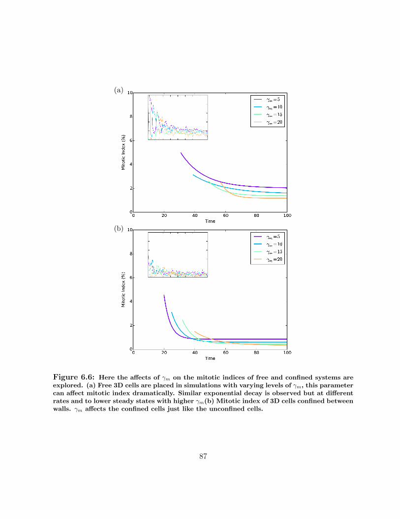
Figure 6.6: Here the affects of γm on the mitotic indices of free and confined systems areexplored. (a) Free 3D cells are placed in simulations with varying levels of γm, this parametercan affect mitotic index dramatically. Similar exponential decay is observed but at differentrates and to lower steady states with higher γm(b) Mitotic index of 3D cells confined betweenwalls. γm affects the confined cells just like the unconfined cells.

87

Figure 6.7: These figures show a two dimensional cross section done halfway in betweenthe confining walls. (a) Voronoi tessellation that was used to determine the number ofneighbours each cell has. Cells with four neighbours are coloured white, pentagonal cells arecoloured green, hexagonal cells are coloured red, heptagonal cyan, and octagonal magenta.(b) This figures shows the cross section of the mass points that make up the cells. Thisimages were generated by taking the projection of all points on a plan parallel to the wallsto simulate an epithelium.

88

Figure 6.8: (a)This figure the fraction of cell polygon types for a number of species.The number in brackets is the number of cells counted, and the GPNP model refers tothe results of a topological model (see Section 3.2.3) that was used by Gibson et al. [151].Taken from[204], c© 2011 Sandersius et al., CC license. (b) Similar measurement using the2D model done by Mkrtchyan et al. [15] at various values of γext, with comparison withDrosophila [158].

89

Figure 6.9: All measurements were done with γm = 5. (a) The change in fraction of polygonsover the simulation time of γext = 15. Cell growth was halted at t = 100TDiv, the system thenrelaxes by rearranging cell distribution towards more favourable packing distribution. (b)The packing distribution at different γext compared to a experimental measurement [158].Inset shows the change in fraction of hexagons over simulation time, cell division was haltedat t = 100TDiv. Error bars are the variation in packing from t = 100TDiv and onward. Mostvalues of γext, except γext = 20 produce distributions comparable to the results shown inFigure 6.8.

90

Figure 6.10: γm has a different effect on packing. All of these measurements were done atγext = 2 to minimize its effects while still maintaining a modicum of intercellular adhesion.(a) The evolution of the fractions of different polygon types over the simulation time, growthwas halted at t = 100. (b) The proportions of different polygon types measured with variousγm, inset shows evolution of hexagonal cell fraction over time. This figure indicates thatwhile γm does affect the distribution, it is γext that is instrumental in this process. γm slowsall cell motion down, while γext only hinders rearrangement.

91

Chapter 7

Conclusions

The goal of this project was to develop a novel method of cell modelling. Some of theexisting models were described in Chapter 3, and the problems associated with themdiscussed. It was found that these models, while excelling in certain situations, wereinsufficient in replicating cell behaviour fully. Due to the complexity of cellular structure,it is difficult to completely simulate cellular behaviour. This problem is compounded bylimitations in computational power. Therefore, the models that have been developed thusfar, were limited by necessity rather than lack of interest or capability. The goal of thisproject was to develop a Molecular Dynamics (MD) based method to simulate cells in amore realistic manner than the techniques used in the field today while taking advantageof the novel computational techniques in the area of scientific computing.

With the use of GPU acceleration, a novel method of modelling cells as three dimen-sional meshes based on previous work by Karttunen, Astrom [14], and Mkrtchyan [15].This method is described was described in some detail in Chapters 5 and 4. The codewas first developed by Jan Westerholm from the Abo Akademi University, then modi-fied to replicate cell behaviour more accurately. GPU acceleration, even though not fullyoptimized yet, has made the run times much more manageable without adding much toresource cost. In this respect, it is the opinion of this author, that the GPU accelerationwas successful and further optimization should be pursued.

Once the simulation was developed, it needed to be validated. After validation, theprogram can be used to study new cells in different ways, and even to make predictions ofcell behaviour. The first step of validation was to compare to the results produced in 2Dby Mkrtchyan et al. in their work [15]. To that end, the behaviour of Mitotic index wasstudied in Chapter 6. It was found that the mitotic indices produced behaved as expected.

92

The simulated cells were also placed in between confining walls to emulate epithelia andto study how the cells packed into two dimensional tissue. It was found that that thesimulation produced expected packing distributions. There is also still more work to bedone towards refining the model further and studying other aspects of cell behaviour.

7.1 Future Plans

The next steps of this project can be divided into three broad areas: Technical improve-ments, further validation, and model refinement. On the technical side progress will bemade on two fronts. There is still some more work that could be done to improve perfor-mance by optimizing the GPU kernels. This will entail algorithmic improvements in theimplementation of MD on GPUs correctly. Some further research will be done into thehardware and software nuances of NVIDIA devices. It is also highly desirable to use otherdevices, such as multicore or Multiple Integrated Core (MIC) devices, for acceleration.GPUs are of course amazing devices, but that is no need to shun other perfectly fine highperformance hardware. This will be done with OpenCL which has the added advantage ofbeing supported by most processors in the in the market.

Further validation and model refinement are related. Firstly, the results in Chapter 6only compare to two dimensional experimental results, the MD method of simulating cellshas to be modified to reproduce cell behaviour in three dimensions. This will be begin byadding cell diffusion to the model. The aim in that case will be to study cell motilities.After that, the next target will be various kinds of cell migration; diffusion directed bysome potential such as a concentration gradient(chemotaxis), changes in adhesion strengthof the Extracellular Matrix (ECM) (haptotaxis). So far only single types of cells havebeen discussed. This model also allows for modelling different types of cells, which leadsto various interesting phenomena such as cell sorting [135] and morphogenesis [134]. Thedifference in cells may be introduced as initial conditions, or changes may be introduce inthe model itself that would affect cell behaviour. The cell division done for this thesis wasrandom symmetric division, but we saw in Chapter 2 that cells may divide different waysto lead to different daughter cells. Asymmetric, and division by the longest axis rule willalso be implemented and their affects on the parameters measured in Chapter 6 will betested and validated.

93

References

[1] D Boal. Mechancis of the Cell. 1st ed. Cambridge University Press, 2002.

[2] H. Lodish. Molecular Cell Biology. Macmillan, 2008.

[3] T. Rozario and D. W. DeSimone. “The extracellular matrix in development andmorphogenesis: A dynamic view”. In: Dev. Biol. 341.1 (2010), pp. 126–140. doi:10.1016/j.ydbio.2009.10.026.

[4] G. K. Gittes. “Developmental biology of the pancreas: A comprehensive review”.In: Dev. Biol. 326.1 (2009), pp. 4–35. doi: 10.1016/j.ydbio.2008.10.024.

[5] T. J. Mitchison and E. D. Salmon. “Mitosis: a history of division.” eng. In: Nat.Cell Biol. 3.1 (2001), E17–E21. doi: 10.1038/35050656.

[6] P. Bheda and R. Schneider. “Epigenetics reloaded: the single-cell revolution”. In:Trends Cell Biol. 24.11 (2014), pp. 712–723. doi: 10.1016/j.tcb.2014.08.010.

[7] D. E. Koshland Jr. “SPECIAL ESSAY: The Seven Pillars of Life”. In: Science295.5563 (2002), pp. 2215–2216. doi: 10.1126/science.1068489.

[8] S. A. Adcock and J. A. McCammon. “Molecular Dynamics: Survey of Methods forSimulating the Activity of Proteins”. In: Chem. Rev. 106.5 (2006), pp. 1589–1615.doi: 10.1021/cr040426m.

[9] J. J. Janke, W. F. D. Bennett, and D. P. Tieleman. “Oleic Acid Phase Behaviorfrom Molecular Dynamics Simulations”. In: Langmuir 30.35 (2014), pp. 10661–10667. doi: 10.1021/la501962n.

[10] W. D. Bennett and D. P. Tieleman. “Computer simulations of lipid membranedomains”. In: Biochim. Biophys. Acta - Biomembranes 1828.8 (2013), pp. 1765–1776. doi: 10.1016/j.bbamem.2013.03.004.

94

[11] J. E. Stone, J. C. Phillips, P. L. Freddolino, D. J. Hardy, L. G. Trabuco, and K.Schulten. “Accelerating Molecular Modeling Applications with Graphics Proces-sors”. In: J. Comput. Chem. 28.16 (Dec. 2007), pp. 2618–2640. doi: 10.1002/jcc.20829.

[12] J. D. Owens, D. Luebke, N. Govindaraju, M. Harris, J. Kruger, A. E. Lefohn, andT. J. Purcell. “A Survey of General-Purpose Computation on Graphics Hardware”.In: Comput. Graph. Forum 26.1 (Mar. 2007), pp. 80–113. doi: 10.1111/j.1467-8659.2007.01012.x.

[13] J. Owens, M. Houston, D. Luebke, S. Green, J. Stone, and J. Phillips. “GPU Com-puting”. In: Proc. IEEE 96.5 (May 2008), pp. 879–899. doi: 10.1109/JPROC.2008.917757.

[14] J. A. Astrom and M. Karttunen. “Cell aggregation: Packing soft grains”. In: PhysicalReview E 73 (6 2006), p. 062301. doi: 10.1103/PhysRevE.73.062301.

[15] A. Mkrtchyan, J. Astrom, and M. Karttunen. “A new model for cell division and mi-gration with spontaneous topology changes”. In: Soft Matter 10.24 (2014), pp. 4332–4339. doi: 10.1039/c4sm00489b.

[16] T. Pollard, W. Earnshaw, and J. Lippincott-Schartz. Cell Biology. Ed. by W.Schmidt. 2nd ed. Saunders Elsevier, 2008.

[17] G. M. Cooper and R. E. Hausman. The Cell. 5th ed. Sinauer Associates, 2000.

[18] D. Voet, J. G. Voet, and C. W. Pratt. Fundamentals of Biochemistry: Life at theMolecular Level. Wiley, 2008.

[19] Q. Wen and P. A. Janmey. “Polymer physics of the cytoskeleton”. In: Curr. Opin.Solid. St. M. 15.5 (2011), 177–182. doi: 10.1016/j.cossms.2011.05.002.

[20] H. Herrmann, H. Bar, L. Kreplak, S. V. Strelkov, and U. Aebi. “Intermediate fila-ments: from cell architecture to nanomechanics”. In: Nat. Rev. Mol. Cell Biol. 8.7(2007), pp. 562–573. doi: 10.1038/nrm2197.

[21] J. I. Castrillo, L. A. Zeef, D. C. Hoyle, N. Zhang, A. Hayes, D. C. J. Gardner,M. J. Cornell, J. Petty, L. Hakes, L. Wardleworth, B. Rash, M. Brown, W. B.Dunn, D. Broadhurst, K. O’Donoghue, S. S. Hester, T. P. J. Dunkley, S. R. Hart,N. Swainston, P. Li, S. J. Gaskell, N. W. Paton, K. S. Lilley, D. B. Kell, and S. G.Oliver. “Growth control of the eukaryote cell: a systems biology study in yeast.”eng. In: J. Biol. 6.2 (2007), p. 4. doi: 10.1186/jbiol54.

[22] L. H. Hartwell. “Cell division from a genetic perspective.” eng. In: J. Cell Biol. 77.3(1978), pp. 627–637.

95

[23] B. Guo, Q. Liang, L. Li, Z. Hu, F. Wu, P. Zhang, Y. Ma, B. Zhao, A. L. Kovcs,Z. Zhang, and et al. “O-GlcNAc-modification of SNAP-29 regulates autophagosomematuration”. In: Nat. Cell Biol. (2014). doi: 10.1038/ncb3066.

[24] S. J. Silverman, A. A. Petti, N. Slavov, L. Parsons, R. Briehof, S. Y. Thiberge, D.Zenklusen, S. J. Gandhi, D. R. Larson, R. H. Singer, and et al. “Metabolic cycling insingle yeast cells from unsynchronized steady-state populations limited on glucoseor phosphate”. In: Proc. Natl. Acad. Sci. U. S. A. 107.15 (2010), pp. 6946–6951.doi: 10.1073/pnas.1002422107.

[25] A. D. Chalmers. “Oriented cell divisions asymmetrically segregate aPKC and gener-ate cell fate diversity in the early Xenopus embryo”. In: Development 130.12 (2003),26572668. doi: 10.1242/dev.00490.

[26] H. Zhang and Z. Z. Wang. “Mechanisms that mediate stem cell self-renewal anddifferentiation.” eng. In: J. Cell. Biochem. 103.3 (2008), pp. 709–718. doi: 10.1002/jcb.21460.

[27] J. A. Knoblich. “Assymetric Cell Division During Animal Development”. In: Nat.Rev. Mol. Cell Biol. 2.1 (2001), pp. 11–20. doi: 10.1038/35048085.

[28] R. A. Neumuller and J. A. Knoblich. “Dividing cellular asymmetry: asymmetric celldivision and its implications for stem cells and cancer”. In: Genes & Development23.23 (2009), pp. 2675–2699. doi: 10.1101/gad.1850809.

[29] Y. Miyaoka and A. Miyajima. “To divide or not to divide: revisiting liver regener-ation”. In: Cell Div 8.1 (2013), p. 8. doi: 10.1186/1747-1028-8-8.

[30] T. Gillies and C. Cabernard. “Cell Division Orientation in Animals”. In: Curr. Biol.21.15 (Aug. 2011), pp. 599–609. doi: 10.1016/j.cub.2011.06.055.

[31] D. Hanahan and R. A. Weinberg. “Hallmarks of cancer: the next generation.” eng.In: Cell 144.5 (2011), pp. 646–674. doi: 10.1016/j.cell.2011.02.013.

[32] H. R. Horvitz and I. Herskowitz. “Mechanisms of asymmetric cell division: two Bsor not two Bs, that is the question.” eng. In: Cell 68.2 (1992), pp. 237–255.

[33] M. Tian, J. R. Neil, and W. P. Schiemann. “Transforming growth factor-β and thehallmarks of cancer.” eng. In: Cell. Signal. 23.6 (2011), pp. 951–962. doi: 10.1016/j.cellsig.2010.10.015.

[34] W. Flemming. Zellsubstanz, kern und zelltheilung. Leipzig, F.C.W Vogel, 1882.

[35] M. P. Stewart, J. Helenius, Y. Toyoda, S. P. Ramanathan, D. J. Muller, and A. A.Hyman. “Hydrostatic pressure and the actomyosin cortex drive mitotic cell round-ing”. In: Nature 469.7329 (2011), 226230. doi: 10.1038/nature09642.

96

[36] T. Lecuit and P.-F. Lenne. “Cell surface mechanics and the control of cell shape, tis-sue patterns and morphogenesis”. In: Nat. Rev. Mol. Cell Biol. 8.8 (2007), pp. 633–644. doi: 10.1038/nrm2222.

[37] C. Roubinet, P. T. Tran, and M. Piel. “Common mechanisms regulating cell cortexproperties during cell division and cell migration.” eng. In: Cytoskeleton (Hoboken)69.11 (2012), pp. 957–972. doi: 10.1002/cm.21086.

[38] S. W. Grill. “Forced to Be Unequal”. In: Science 330.6004 (2010), 597598. doi:10.1126/science.1198343.

[39] Y. Imoto, Y. Yoshida, F. Yagisawa, H. Kuroiwa, and T. Kuroiwa. “The cell cycle,including the mitotic cycle and organelle division cycles, as revealed by cytologicalobservations”. In: Microscopy 60.suppl 1 (2011), S117S136. doi: 10.1093/jmicro/dfr034.

[40] P. Kunda and B. Baum. “The actin cytoskeleton in spindle assembly and position-ing.” eng. In: Trends Cell Biol. 19.4 (2009), pp. 174–179. doi: 10.1016/j.tcb.2009.01.006.

[41] M. T. Tyree and H. T. Hammel. “The Measurement of the Turgor Pressure and theWater Relations of Plants by the Pressure-bomb Technique”. In: J. Exp. Bot. 23.1(1972), 267282. doi: 10.1093/jxb/23.1.267.

[42] N. Minc, D. Burgess, and F. Chang. “Influence of Cell Geometry on Division-PlanePositioning”. In: Cell 144.3 (2011), pp. 414–426. doi: 10.1016/j.cell.2011.01.016.

[43] R. Rappaport. Cytokinesis in Animal Cells. Cambridge University Press, 1996.

[44] J. M. Scholey, I. Brust-Mascher, and A. Mogilner. “Cell division.” eng. In: Nature422.6933 (2003), pp. 746–752. doi: 10.1038/nature01599.

[45] O. Hertwig. Das Problem der Befruchtung und der Isotropie des Eies, eine Theorieder Vererbung. Jena, 1884.

[46] D. St Johnston and J. Ahringer. “Cell Polarity in Eggs and Epithelia: Parallels andDiversity”. In: Cell 141.5 (2010), pp. 757–774. doi: 10.1016/j.cell.2010.05.011.

[47] Y. N. Jan and L. Y. Jan. “Assymetric cell division”. In: Nature 392.6678 (1998),pp. 775–778. doi: 10.1038/33854.

[48] J. A. Knoblich. “Mechanisms of Asymmetric Stem Cell Division”. In: Cell 132.4(2008), pp. 583–597. doi: 10.1016/j.cell.2008.02.007.

[49] A. Mkrtchyan. “A Single Cell Based Model for Cell Divisions with Spontaneoustopology changes”. PhD thesis. 2013.

97

[50] B. M. Gumbiner. “Cell adhesion: the molecular basis of tissue architecture andmorphogenesis.” eng. In: Cell 84.3 (1996), pp. 345–357.

[51] G. Bell, M. Dembo, and P. Bongrand. “Cell adhesion. Competition between non-specific repulsion and specific bonding”. In: Biophys. J. 45.6 (1984), 10511064. doi:10.1016/s0006-3495(84)84252-6.

[52] C. D. Buckley, G. E. Rainger, P. F. Bradfield, G. B. Nash, and D. L. Simmons.“Cell adhesion: More than just glue (Review)”. In: Mol. Membr. Biol. 15.4 (1998),167176. doi: 10.3109/09687689709044318.

[53] J. T. Parsons, A. R. Horwitz, and M. A. Schwartz. “Cell adhesion: integratingcytoskeletal dynamics and cellular tension.” eng. In: Nat. Rev. Mol. Cell Biol. 11.9(2010), pp. 633–643. doi: 10.1038/nrm2957.

[54] J. Kafer, T. Hayashi, A. F. M. Maree, R. W. Carthew, and F. Graner. “Cell adhe-sion and cortex contractility determine cell patterning in the Drosophilaretina”. In:Proc. Natl. Acad. Sci. U. S. A. 104.47 (2007), 1854918554. doi: 10.1073/pnas.0704235104.

[55] P. DiMilla, K. Barbee, and D. Lauffenburger. “Mathematical model for the effectsof adhesion and mechanics on cell migration speed”. In: Biophys. J. 60.1 (1991),1537. doi: 10.1016/s0006-3495(91)82027-6.

[56] T. Hayashi and R. W. Carthew. “Surface mechanics mediate pattern formationin the developing retina”. In: Nature 431.7009 (2004), 647652. doi: 10 . 1038 /

nature02952.

[57] H. Byrne and D. Drasdo. “Individual-based and continuum models of growing cellpopulations: a comparison”. In: J. Math. Biol. 58.4-5 (2008), 657687. doi: 10.1007/s00285-008-0212-0.

[58] D. Stamenovic and D. E. Ingber. “Models of cytoskeletal mechanics of adherentcells.” eng. In: Biomech. Model. Mechanobiol. 1.1 (2002), pp. 95–108. doi: 10.

1007/s10237-002-0009-9.

[59] B. G. Sengers, M. Taylor, C. P. Please, and R. O. C. Oreffo. “Computational mod-elling of cell spreading and tissue regeneration in porous scaffolds.” eng. In: Bioma-terials 28.10 (2007), pp. 1926–1940. doi: 10.1016/j.biomaterials.2006.12.008.

[60] A. Voss-Bohme. “Multi-Scale Modeling in Morphogenesis: A Critical Analysis of theCellular Potts Model”. In: PLoS ONE 7.9 (2012). Ed. by C. M. Aegerter, e42852.doi: 10.1371/journal.pone.0042852.

98

[61] A. B. Patel, W. T. Gibson, M. C. Gibson, and R. Nagpal. “Modeling and InferringCleavage Patterns in Proliferating Epithelia”. In: PLoS Comput. Biol. 5.6 (2009).Ed. by J. Axelrod, e1000412. doi: 10.1371/journal.pcbi.1000412.

[62] A. J. Kabla. “Collective cell migration: leadership, invasion and segregation”. en.In: Journal of The Royal Society Interface 9.77 (Dec. 2012), pp. 3268–3278. doi:10.1098/rsif.2012.0448.

[63] T. J. Newman. “Modeling multicellular systems using subcellular elements.” eng.In: Math. Biosci. Eng. 2.3 (2005), pp. 613–624.

[64] T. Beyer and M. Meyer-Hermann. “Multiscale modeling of cell mechanics and tissueorganization”. In: 28.2 (2009), 3845. doi: 10.1109/memb.2009.931790.

[65] J. A. Anderson, C. D. Lorenz, and A. Travesset. “General purpose molecular dy-namics simulations fully implemented on graphics processing units”. In: J. Comput.Phys. 227.10 (May 2008), pp. 5342–5359. doi: 10.1016/j.jcp.2008.01.047.

[66] S. Plimpton. “Fast Parallel Algorithms for Short-Range Molecular Dynamics”. In:J. Comput. Phys. 117.1 (Mar. 1995), pp. 1–19. doi: 10.1006/jcph.1995.1039.

[67] W Smith and T. R. Forester. “DL POLY 2.0: a general-purpose parallel moleculardynamics simulation package.” In: J. Mol. Graph. 14.3 (June 1996), pp. 136–41.

[68] H. Berendsen, D. van der Spoel, and R. van Drunen. “GROMACS: A message-passing parallel molecular dynamics implementation”. In: Comput. Phys. Commun.91.1-3 (Sept. 1995), pp. 43–56. doi: 10.1016/0010-4655(95)00042-E.

[69] J. C. Phillips, R. Braun, W. Wang, J. Gumbart, E. Tajkhorshid, E. Villa, C. Chipot,R. D. Skeel, L. Kale, and K. Schulten. “Scalable molecular dynamics with NAMD.”In: J. Comput. Chem. 26.16 (Dec. 2005), pp. 1781–802. doi: 10.1002/jcc.20289.

[70] H. Limbach, A. Arnold, B. Mann, and C. Holm. “ESPResSoan extensible simulationpackage for research on soft matter systems”. In: Comput. Phys. Commun. 174.9(May 2006), pp. 704–727. doi: 10.1016/j.cpc.2005.10.005.

[71] K. Hinsen. “The molecular modeling toolkit: A new approach to molecular simula-tions”. In: J. Comput. Chem. 21.2 (Jan. 2000), pp. 79–85. doi: 10.1002/(SICI)1096-987X(20000130)21:2<79::AID-JCC1>3.0.CO;2-B.

[72] B. J. Alder and T. E. Wainwright. “Phase Transition for a Hard Sphere System”.In: J. Chem. Phys. 27.5 (1957), p. 1208. doi: 10.1063/1.1743957.

[73] A. Rahman. “Correlations in the Motion of Atoms in Liquid Argon”. In: Phys. Rev.136.2A (Oct. 1964), A405–A411. doi: 10.1103/PhysRev.136.A405.

99

[74] R. Allen, F. de Wette, and A. Rahman. “Calculation of Dynamical Surface Proper-ties of Noble-Gas Crystals. II. Molecular Dynamics”. In: Phys. Rev. 179.3 (1969),887891. doi: 10.1103/physrev.179.887.

[75] B. J. Alder and T. E. Wainwright. “Studies in Molecular Dynamics. VIII. TheTransport Coefficients for a Hard-Sphere Fluid”. In: J. Chem. Phys. 53.10 (1970),p. 3813. doi: 10.1063/1.1673845.

[76] J. A. McCammon, B. R. Gelin, and M. Karplus. “Dynamics of folded proteins”. In:Nature 267.5612 (1977), 585590. doi: 10.1038/267585a0.

[77] W. D. Bennett, A. W. Chen, S. Donnini, G. Groenhof, and D. P. Tieleman. “Con-stant pH simulations with the coarse-grained MARTINI model – Application tooleic acid aggregates”. In: Can. J. Chem. 91.9 (Apr. 2013), pp. 839–846. doi:10.1139/cjc-2013-0010.

[78] N. Nisoh, M. Karttunen, L. Monticelli, and J. Wong-ekkabut. “Lipid monolayerdisruption caused by aggregated carbon nanoparticles”. In: RSC Adv. 5.15 (2015),1167611685. doi: 10.1039/c4ra17006g.

[79] B. Liu, M. I. Hoopes, and M. Karttunen. “Molecular Dynamics Simulations ofDPPC/CTAB Monolayers at the Air/Water Interface”. In: J. Phys. Chem. B 118.40(2014), 1172311737. doi: 10.1021/jp5050892.

[80] W. Bennett, N. Sapay, and D. Tieleman. “Atomistic Simulations of Pore Formationand Closure in Lipid Bilayers”. In: Biophys. J. 106.1 (2014), 210219. doi: 10.1016/j.bpj.2013.11.4486.

[81] T. N. Do, W.-Y. Choy, and M. Karttunen. “Accelerating the Conformational Sam-pling of Intrinsically Disordered Proteins”. In: J. Chem. Theory Comput. 10.11(2014), 50815094. doi: 10.1021/ct5004803.

[82] A. H. Elcock. “Molecular simulations of diffusion and association in multimacro-molecular systems.” eng. In: Methods Enzymol. 383 (2004), pp. 166–198. doi: 10.1016/S0076-6879(04)83008-8.

[83] A. Warshel. “Computer simulations of enzyme catalysis: methods, progress, andinsights.” eng. In: Annu. Rev. Biophys. Biomol. Struct. 32 (2003), pp. 425–443.doi: 10.1146/annurev.biophys.32.110601.141807.

[84] W. F. van Gunsteren and H. J. C. Berendsen. “Computer Simulation of MolecularDynamics: Methodology, Applications, and Perspectives in Chemistry”. In: Angew.Chem. Int. Ed. Engl. 29.9 (1990), pp. 992–1023. doi: 10.1002/anie.199009921.

100

[85] J.-P. Ryckaert and A. Bellemans. “Molecular dynamics of liquid alkanes”. In: Fara-day Discuss. Chem. Soc. 66 (1978), p. 95. doi: 10.1039/dc9786600095.

[86] J.-P. Ryckaert, G. Ciccotti, and H. J. Berendsen. “Numerical integration of thecartesian equations of motion of a system with constraints: molecular dynamicsof n-alkanes”. In: J. Comput. Phys. 23.3 (1977), 327341. doi: 10.1016/0021-

9991(77)90098-5.

[87] D. Frenkel, B. Smit, and M. A. Ratner. “Understanding Molecular Simulation: FromAlgorithms to Applications”. In: Phys. Today 50.7 (1997), p. 66. doi: 10.1063/1.881812.

[88] T. Darden, D. York, and L. Pedersen. “Particle mesh Ewald: An Nlog(N) methodfor Ewald sums in large systems”. In: J. Chem. Phys. 98.12 (1993), p. 10089. doi:10.1063/1.464397.

[89] P. P. Ewald. “Die Berechnung optischer und elektrostatischer Gitterpotentiale”. In:Annalen der Physik 369.3 (1921), pp. 253–287. doi: 10.1002/andp.19213690304.

[90] W. M. Brown, A. Kohlmeyer, S. J. Plimpton, and A. N. Tharrington. “Implement-ing molecular dynamics on hybrid high performance computers Particleparticleparticle-mesh”. In: Comput. Phys. Commun. 183.3 (Mar. 2012), pp. 449–459. doi:10.1016/j.cpc.2011.10.012.

[91] U. Essmann, L. Perera, M. L. Berkowitz, T. Darden, H. Lee, and L. G. Pedersen. “Asmooth particle mesh Ewald method”. In: J. Chem. Phys. 103.19 (1995), p. 8577.doi: 10.1063/1.470117.

[92] R. W. Hockney and K. W. Eastwood. Computer Simulations Using Particles. CRCPress, 2010.

[93] M. Karttunen, J. Rottler, I. Vattulainen, and C. Sagui. “Chapter 2 Electrostaticsin Biomolecular Simulations: Where Are We Now and Where Are We Heading?”In: Curr. Top. Membr. (2008), pp. 49–89. doi: 10.1016/s1063-5823(08)00002-1.

[94] G. A. Cisneros, M. Karttunen, P. Ren, and C. Sagui. “Classical Electrostatics forBiomolecular Simulations”. In: Chem. Rev. 114.1 (2014), pp. 779–814. doi: 10.

1021/cr300461d.

[95] T. Murtola, A. Bunker, I. Vattulainen, M. Deserno, and M. Karttunen. “Multiscalemodeling of emergent materials: biological and soft matter”. In: Phys. Chem. Chem.Phys. 11.12 (2009), p. 1869. doi: 10.1039/b818051b.

101

[96] D. Tieleman, S. Marrink, and H. Berendsen. “A computer perspective of mem-branes: molecular dynamics studies of lipid bilayer systems”. In: Biochimica etBiophysica Acta (BBA) - Reviews on Biomembranes 1331.3 (1997), 235270. doi:10.1016/s0304-4157(97)00008-7.

[97] L. Monticelli, S. K. Kandasamy, X. Periole, R. G. Larson, D. P. Tieleman, and S.-J.Marrink. “The MARTINI Coarse-Grained Force Field: Extension to Proteins”. In:J. Chem. Theory Comput. 4.5 (2008), 819834. doi: 10.1021/ct700324x.

[98] S. J. Marrink, H. J. Risselada, S. Yefimov, D. P. Tieleman, and A. H. de Vries. “TheMARTINI Force Field: Coarse Grained Model for Biomolecular Simulations”. In: J.Phys. Chem. B 111.27 (2007), 78127824. doi: 10.1021/jp071097f.

[99] Y. Wang, W. Jiang, T. Yan, and G. A. Voth. “Understanding ionic liquids throughatomistic and coarse-grained molecular dynamics simulations.” In: Acc. Chem. Res.40.11 (Nov. 2007), pp. 1193–9. doi: 10.1021/ar700160p.

[100] R. Rudd and J. Broughton. “Coarse-grained molecular dynamics and the atomiclimit of finite elements”. In: Phys. Rev. B 58.10 (Sept. 1998), R5893–R5896. doi:10.1103/PhysRevB.58.R5893.

[101] L. Verlet. “Computer Experiments on Classical Fluids. I. Thermodynamical Prop-erties of Lennard-Jones Molecules”. In: Phys. Rev. 159.1 (1967), 98103. doi: 10.1103/physrev.159.98.

[102] E. Hairer, C. Lubich, and G. Wanner. “Geometric numerical integration illustratedby the StrmerVerlet method”. In: Acta Numerica 12 (2003), 399450. doi: 10.1017/s0962492902000144.

[103] I. Geudens and H. Gerhardt. “Coordinating cell behaviour during blood vessel for-mation”. In: Development 138.21 (2011), 45694583. doi: 10.1242/dev.062323.

[104] K. Riento and A. J. Ridley. “Rocks: multifunctional kinases in cell behaviour”. In:Nat. Rev. Mol. Cell Biol. 4.6 (2003), 446456. doi: 10.1038/nrm1128.

[105] M. C. Frame. “Src in cancer: deregulation and consequences for cell behaviour”. In:Biochimica et Biophysica Acta (BBA) - Reviews on Cancer 1602.2 (2002), 114130.doi: 10.1016/s0304-419x(02)00040-9.

[106] R. M. Merks and J. A. Glazier. “A cell-centered approach to developmental biology”.In: Physica A: Statistical Mechanics and its Applications 352.1 (2005), 113130. doi:10.1016/j.physa.2004.12.028.

[107] S. Turner. “Using cell potential energy to model the dynamics of adhesive biologicalcells”. In: Phys. Rev. E 71 (4 2005), p. 041903. doi: 10.1103/PhysRevE.71.041903.

102

[108] N. Bellomo and B. Carbonaro. “Toward a mathematical theory of living systemsfocusing on developmental biology and evolution: A review and perspectives”. In:Phys. Life Rev. 8.1 (2011), 118. doi: 10.1016/j.plrev.2010.12.001.

[109] N. NDri, W. Shyy, and R. Tran-Son-Tay. “Computational Modeling of Cell Adhe-sion and Movement Using a Continuum-Kinetics Approach”. In: Biophys. J. 85.4(2003), 22732286. doi: 10.1016/s0006-3495(03)74652-9.

[110] D. A. Baltazar and A. Friedman. Models of Cellular Regulation. Oxford UniversityPress (OUP), 2008.

[111] J. C. Sible and J. J. Tyson. “Mathematical modeling as a tool for investigating cellcycle control networks”. In: Methods 41.2 (2007), pp. 238–247. doi: 10.1016/j.ymeth.2006.08.003.

[112] J. A. D. Wattis, B. O’Malley, H. Blackburn, L. Pickersgill, J. Panovska, H. M.Byrne, and K. G. Jackson. “Mathematical model for low density lipoprotein (LDL)endocytosis by hepatocytes.” eng. In: Bull. Math. Biol. 70.8 (2008), pp. 2303–2333.doi: 10.1007/s11538-008-9347-9.

[113] R. Robeva, R. Davies, T. Hodge, and A. Enyedi. “Mathematical biology modulesbased on modern molecular biology and modern discrete mathematics.” eng. In:CBE Life Sci. Educ. 9.3 (2010), pp. 227–240. doi: 10.1187/cbe.10-03-0019.

[114] N. F. Britton. Essential mathematical biology. Springer, 2003.

[115] J. D. Murray. Mathematical Biology: I. An Introduction: Pt. 1 (InterdisciplinaryApplied Mathematics). Springer New York, 2008.

[116] J. Schnute. “A Versatile Growth Model with Statistically Stable Parameters”. In:Can. J. Fish. Aquat. Sci. 38.9 (1981), 11281140. doi: 10.1139/f81-153.

[117] M. H. Zwietering, I. Jongenburger, F. M. Rombouts, and K. van ’t Riet. “Model-ing of the bacterial growth curve.” eng. In: Appl. Environ. Microbiol. 56.6 (1990),pp. 1875–1881.

[118] F. J. Richards. “A Flexible Growth Function for Empirical Use”. In: J. Exp. Bot.10.2 (1959), pp. 290–301. doi: 10.1093/jxb/10.2.290. eprint: http://jxb.oxfordjournals.org/content/10/2/290.full.pdf+html.

[119] G. C. Jahn, L. P. Almazan, and J. B. Pacia. “Effect of Nitrogen Fertilizer on theIntrinsic Rate of Increase of Hysteroneura setariae (Thomas) (Homoptera: Aphidi-dae) on Rice (Oryza sativa L.)” In: Environmental Entomology 34.4 (2005), 938943.doi: 10.1603/0046-225x-34.4.938.

103

[120] B. Gompertz. “On the nature of the function expressive of the law of human mor-tality, and on a new mode of determining the value of life contingencies”. In: Philos.Trans. Roy. Soc. London (1825), pp. 513–583.

[121] M. Ben Amar, C. Chatelain, and P. Ciarletta. “Contour Instabilities in Early TumorGrowth Models”. In: Phys. Rev. Lett. 106.14 (2011). doi: 10.1103/physrevlett.106.148101.

[122] J. Ranft, M. Basan, J. Elgeti, J.-F. Joanny, J. Prost, and F. Julicher. “Fluidizationof tissues by cell division and apoptosis”. en. In: Proc. Natl. Acad. Sci. U. S. A.107.49 (Dec. 2010), pp. 20863–20868. doi: 10.1073/pnas.1011086107.

[123] T. Bittig, O. Wartlick, A. Kicheva, M. Gonzalez-Gaitn, and F. Jlicher. “Dynamicsof anisotropic tissue growth”. In: New Journal of Physics 10.6 (2008), p. 063001.doi: 10.1088/1367-2630/10/6/063001.

[124] G. Schaller and M. Meyer-Hermann. “Multicellular tumor spheroid in an off-latticeVoronoi-Delaunay cell model”. In: Phys. Rev. E 71.5 (2005). doi: 10.1103/physreve.71.051910.

[125] G. Schaller and M. Meyer-Hermann. “Kinetic and dynamic Delaunay tetrahedral-izations in three dimensions”. In: Comput. Phys. Commun. 162.1 (2004), 923. doi:10.1016/j.cpc.2004.06.066.

[126] M. Meyer-Hermann. “Delaunay-Object-Dynamics: Cell Mechanics with a 3D Ki-netic and Dynamic Weighted Delaunay-Triangulation”. In: Curr. Top. Dev. Biol.(2008), 373399. doi: 10.1016/s0070-2153(07)81013-1.

[127] D. T. Lee and B. J. Schachter. “Two algorithms for constructing a Delaunay trian-gulation”. In: International Journal of Computer & Information Science 9.3 (1980),219242. doi: 10.1007/bf00977785.

[128] L. Paul Chew. “Constrained delaunay triangulations”. In: Algorithmica 4.1-4 (1989),97108. doi: 10.1007/bf01553881.

[129] H. Edelsbrunner and N. R. Shah. “Incremental topological flipping works for regulartriangulations”. In: Algorithmica 15.3 (1996), 223241. doi: 10.1007/bf01975867.

[130] B. Delaunay. “Sur la sphere vide. A la memoire de Georges Voronoı”. In: Bulletinde l’Academie des Sciences de l’URSS 6 (1934), pp. 793–800.

[131] F. Aurenhammer. “Power Diagrams: Properties, Algorithms and Applications”. In:SIAM Journal on Computing 16.1 (1987), 7896. doi: 10.1137/0216006.

104

[132] T. Beyer and M. Meyer-Hermann. “Modeling emergent tissue organization involvinghigh-speed migrating cells in a flow equilibrium”. en. In: Phys .Rev. E 76.2 (Aug.2007), p. 021929. doi: 10.1103/PhysRevE.76.021929.

[133] A. Szabo and R. M. H. Merks. “Cellular Potts Modeling of Tumor Growth, TumorInvasion, and Tumor Evolution”. In: Front. Oncol. 3 (2013). doi: 10.3389/fonc.2013.00087.

[134] J. Glazier and F. Graner. “Simulation of the differential adhesion driven rearrange-ment of biological cells”. In: Phys. Rev. E 47.3 (1993), pp. 2128–2154. doi: 10.1103/physreve.47.2128.

[135] F. Graner and J. Glazier. “Simulation of biological cell sorting using a two-dimensionalextended Potts model”. In: Phys. Rev. Lett. 69.13 (1992), pp. 2013–2016. doi:10.1103/physrevlett.69.2013.

[136] R. B. Potts and C. Domb. “Some generalized order-disorder transformations”. In:Math. Proc. Camb. Phil. Soc. 48.01 (1952), pp. 106–109. doi: 10.1017/s0305004100027419.

[137] E. Ising. “Beitrag zur theorie des ferromagnetismus”. In: Zeitschrift fur Physik AHadrons and Nuclei 31.1 (1925), pp. 253–258.

[138] F. Y. Wu. “The Potts model”. In: Rev. Mod. Phys. 54.1 (1982), pp. 235–268. doi:10.1103/revmodphys.54.235.

[139] N. Chen, J. A. Glazier, J. A. Izaguirre, and M. S. Alber. “A parallel implementationof the Cellular Potts Model for simulation of cell-based morphogenesis”. In: Comput.Phys. Commun. 176.11-12 (2007), pp. 670–681. doi: 10.1016/j.cpc.2007.03.007.

[140] N. Metropolis and S. Ulam. “The Monte Carlo Method”. In: J. Am. Stat. Assoc.44.247 (1949), pp. 335–341. doi: 10.1080/01621459.1949.10483310.

[141] N. Metropolis. “The beginning of the Monte Carlo method”. In: Los Alamos Science15.584 (1987), pp. 125–130.

[142] A. Kohn-Luque, W. de Back, J. Starru, A. Mattiotti, A. Deutsch, J. M. Prez-Pomares, and M. A. Herrero. “Early Embryonic Vascular Patterning by Matrix-Mediated Paracrine Signalling: A Mathematical Model Study”. In: PLoS ONE 6.9(2011). Ed. by B. Riley, e24175. doi: 10.1371/journal.pone.0024175.

[143] M. Krieg, Y. Arboleda-Estudillo, P.-H. Puech, J. Kfer, F. Graner, D. J. Mller, andC.-P. Heisenberg. “Tensile forces govern germ-layer organization in zebrafish”. In:Nat. Cell Biol. 10.4 (2008), 429436. doi: 10.1038/ncb1705.

105

[144] J. Starruß, T. Bley, L. Søgaard-Andersen, and A. Deutsch. “A New Mechanismfor Collective Migration in Myxococcus xanthus”. In: J Stat Phys 128.1-2 (2007),269286. doi: 10.1007/s10955-007-9298-9.

[145] R. M. H. Merks, E. D. Perryn, A. Shirinifard, and J. A. Glazier. “Contact-InhibitedChemotaxis in De Novo and Sprouting Blood-Vessel Growth”. In: PLoS Comput.Biol. 4.9 (2008). Ed. by P. E. Bourne, e1000163. doi: 10.1371/journal.pcbi.1000163.

[146] J. Kafer, P. Hogeweg, and A. F. M. Mare. “Moving Forward Moving Backward:Directional Sorting of Chemotactic Cells due to Size and Adhesion Differences”. In:PLoS Comp Biol 2.6 (2006), e56. doi: 10.1371/journal.pcbi.0020056.

[147] R. J. Matela and R. J. Fletterick. “Computer simulation of cellular self-sorting: Atopological exchange model”. In: J. Theor. Biol. 84.4 (1980), 673690. doi: 10.1016/s0022-5193(80)80027-0.

[148] R. J. Matela and R. J. Fletterick. “A topological exchange model for cell self-sorting”. In: J. Theor. Biol. 76.4 (1979), 403414. doi: 10.1016/0022-5193(79)90009-2.

[149] S. Duvdevani-Bar and L. Segel. “On Topological Simulations in Developmental Bi-ology”. In: J. Theor. Biol. 166.1 (1994), 3350. doi: 10.1006/jtbi.1994.1003.

[150] A Tardieu and M Delaye. “Eye Lens Proteins and Transparency: From Light Trans-mission Theory to Solution X-Ray Structural Analysis”. In: Annu. Rev. Biophys.Biophys. Chem. 17.1 (1988), 4770. doi: 10.1146/annurev.bb.17.060188.000403.

[151] M. C. Gibson, A. B. Patel, R. Nagpal, and N. Perrimon. “The emergence of geomet-ric order in proliferating metazoan epithelia”. In: Nature 442.7106 (2006), 10381041.doi: 10.1038/nature05014.

[152] F. T. Lewis. “The effect of cell division on the shape and size of hexagonal cells”.In: The Anatomical Record 33.5 (1926), 331355. doi: 10.1002/ar.1090330502.

[153] Y.-i. Nakajima, E. J. Meyer, A. Kroesen, S. A. McKinney, and M. C. Gibson.“Epithelial junctions maintain tissue architecture by directing planar spindle orien-tation”. In: Nature 500.7462 (2013), 359362. doi: 10.1038/nature12335.

[154] R. Nagpal, A. Patel, and M. C. Gibson. “Epithelial topology”. In: Bioessays 30.3(2008), 260266. doi: 10.1002/bies.20722.

[155] P. M. Morse. “Diatomic Molecules According to the Wave Mechanics. II. VibrationalLevels”. In: Phys. Rev. 34.1 (1929), 5764. doi: 10.1103/physrev.34.57.

106

[156] F. van Roy and G. Berx. “The cell-cell adhesion molecule E-cadherin.” eng. In: Cell.Mol. Life Sci. 65.23 (2008), pp. 3756–3788. doi: 10.1007/s00018-008-8281-1.

[157] M. P. Stemmler. “Cadherins in development and cancer.” eng. In: Mol. Biosyst. 4.8(2008), pp. 835–850. doi: 10.1039/b719215k.

[158] O. Wartlick, P. Mumcu, A. Kicheva, T. Bittig, C. Seum, F. Julicher, and M.Gonzalez-Gaitan. “Dynamics of Dpp Signaling and Proliferation Control”. In: Sci-ence 331.6021 (2011), 11541159. doi: 10.1126/science.1200037.

[159] A. Mkrtchyan, P. Madhikar, J. Astrom, and M. Karttunen. “Working title:Effectsof Cell Division Variance on Epithelial Topologies.” In: Manuscript to be submitted.(2015).

[160] H. Sutter. “The free lunch is over: A fundamental turn toward concurrency in soft-ware”. In: Dr. Dobbs journal 30.3 (2005), pp. 202–210.

[161] H. Sutter. Welcome to the Jungle. http://herbsutter.com/welcome-to-the-jungle/. Blog. 2012.

[162] M. Rupp. CPU, GPU and MIC Hardware Characteristics over Time. Blog. 2013.

[163] J. E. Stone, D. Gohara, and G. Shi. “OpenCL: A Parallel Programming Standardfor Heterogeneous Computing Systems.” In: Computing in science & engineering12.3 (May 2010), pp. 66–72. doi: 10.1109/MCSE.2010.69.

[164] J. E. Stone, D. J. Hardy, I. S. Ufimtsev, and K. Schulten. “GPU-accelerated molec-ular modeling coming of age.” In: Journal of molecular graphics & modelling 29.2(Sept. 2010), pp. 116–25. doi: 10.1016/j.jmgm.2010.06.010.

[165] W. Liu, B. Schmidt, G. Voss, and W. Mller-Wittig. “Molecular Dynamics Simula-tions on Commodity GPUs with CUDA”. In: Lecture Notes in Computer Science(2007), 185196. doi: 10.1007/978-3-540-77220-0_20.

[166] J. Yang, Y. Wang, and Y. Chen. “GPU accelerated molecular dynamics simulationof thermal conductivities”. In: J. Comput. Phys. 221.2 (2007), 799804. doi: 10.1016/j.jcp.2006.06.039.

[167] J. L. Klepeis, K. Lindorff-Larsen, R. O. Dror, and D. E. Shaw. “Long-timescalemolecular dynamics simulations of protein structure and function”. In: Curr. Opin.Struct. Biol. 19.2 (2009), 120127. doi: 10.1016/j.sbi.2009.03.004.

[168] A. Sunarso, T. Tsuji, and S. Chono. “GPU-accelerated molecular dynamics sim-ulation for study of liquid crystalline flows”. In: J. Comput. Phys. 229.15 (2010),54865497. doi: 10.1016/j.jcp.2010.03.047.

107

[169] A. W. Gotz, M. J. Williamson, D. Xu, D. Poole, S. Le Grand, and R. C. Walker.“Routine Microsecond Molecular Dynamics Simulations with AMBER on GPUs. 1.Generalized Born.” In: J. Chem. Theory Comput. 8.5 (May 2012), pp. 1542–1555.doi: 10.1021/ct200909j.

[170] R. Salomon-Ferrer, A. W. Gtz, D. Poole, S. Le Grand, and R. C. Walker. “RoutineMicrosecond Molecular Dynamics Simulations with AMBER on GPUs. 2. ExplicitSolvent Particle Mesh Ewald”. In: J. Chem. Theory Comput. 9.9 (2013), 38783888.doi: 10.1021/ct400314y.

[171] J. Nickolls, I. Buck, M. Garland, and K. Skadron. “Scalable parallel programmingwith CUDA”. In: Queue 6.2 (2008), p. 40. doi: 10.1145/1365490.1365500.

[172] S. Cook. CUDA programming: a developer’s guide to parallel computing with GPUs.Newnes, 2012.

[173] J. Hoberock and N. Bell. Thrust. 2008.

[174] Khronos OpenCL Working Group and others. “The opencl specification”. In: version1.29 (2008), p. 8.

[175] C. Nvidia. Programming guide. 2008.

[176] NVIDIA. “NVIDIA’s Next Generation CUDATM Compute Architecture: KeplerTM

GK110”. In: NVIDIA. NVIDIA, 2015, pp. 9–10.

[177] H. Shen. “The compressive mechanical properties of C n (n = 20, 60, 80, 180) andendohedral M@C 60 (M = Na, Al, Fe) fullerene molecules”. In: Mol. Phys. 105.17-18(2007), pp. 2405–2409. doi: 10.1080/00268970701679467.

[178] H. Shen. “Mechanical properties and electronic structures of compressed C60, C180and C60@C180 fullerene molecules”. In: J. Mater. Sci. 42.17 (2007), 73377342. doi:10.1007/s10853-007-1576-z.

[179] P. Fowler and D. Manolopoulos. An Atlas of FULLERENES. Dover Publications,Inc., 2007.

[180] L. Hayflick. “The limited in vitro lifetime of human diploid cell strains”. In: Exp.Cell Res. 37.3 (1965), 614636. doi: 10.1016/0014-4827(65)90211-9.

[181] L. Hayflick and P. Moorhead. “The serial cultivation of human diploid cell strains”.In: Exp. Cell Res. 25.3 (1961), pp. 585–621. doi: 10.1016/0014-4827(61)90192-6.

[182] D. Bakowies, M. Bhl, and W. Thiel. “A density functional study on the shape ofC180 and C240 fullerenes”. In: Chem. Phys. Lett. 247.4-6 (1995), pp. 491–493. doi:10.1016/s0009-2614(95)01222-2.

108

[183] M. Yoshida. M. Yoshida’s Fullerene Library. 1999. url: http://www.jcrystal.com/steffenweber/gallery/Fullerenes/Fullerenes.html.

[184] K. K. Hirschi. “PDGF, TGF-beta , and Heterotypic Cell-Cell Interactions MediateEndothelial Cell-induced Recruitment of 10T1/2 Cells and Their Differentiation toa Smooth Muscle Fate”. In: The Journal of Cell Biology 141.3 (1998), 805814. doi:10.1083/jcb.141.3.805.

[185] A Pierres, A. Benoliel, and P Bongrand. “Cell-cell interactions”. In: Physical chem-istry of biological interfaces (2000), pp. 459–522.

[186] U Rutishauser, A Acheson, A. Hall, D. Mann, and J Sunshine. “The neural cell adhe-sion molecule (NCAM) as a regulator of cell-cell interactions”. In: Science 240.4848(1988), 5357. doi: 10.1126/science.3281256.

[187] H. W. Jones. “Record of the first physician to see Henrietta Lacks at the JohnsHopkins Hospital: History of the beginning of the HeLa cell line”. In: Am. J. Obstet.Gynecol. 176.6 (1997), s227s228. doi: 10.1016/s0002-9378(97)70379-x.

[188] The Johns Hopkins Hospital. Surgical Biopsy Number 92498. Baltimore, MD, 1951.

[189] L. Zhao, C. D. Kroenke, J. Song, D. Piwnica-Worms, J. J. H. Ackerman, and J. J.Neil. “Intracellular water-specific MR of microbead-adherent cells: the HeLa cellintracellular water exchange lifetime”. In: NMR Biomed. 21.2 (2008), 159164. doi:10.1002/nbm.1173.

[190] R. Milo, P. Jorgensen, U. Moran, G. Weber, and M. Springer. “BioNumbers–thedatabase of key numbers in molecular and cell biology”. In: Nucleic Acids Res.38.Database (2009), D750D753. doi: 10.1093/nar/gkp889.

[191] K. Park, J. Jang, D. Irimia, J. Sturgis, J. Lee, J. P. Robinson, M. Toner, and R.Bashir. “’Living cantilever arrays’ for characterization of mass of single live cells influids.” eng. In: Lab. Chip 8.7 (2008), pp. 1034–1041. doi: 10.1039/b803601b.

[192] S. W. Grill and A. A. Hyman. “Spindle positioning by cortical pulling forces.” eng.In: Dev. Cell 8.4 (2005), pp. 461–465. doi: 10.1016/j.devcel.2005.03.014.

[193] J. P. A. Baak, E. Gudlaugsson, I. Skaland, L. H. R. Guo, J. Klos, T. H. Lende,H. Søiland, E. A. M. Janssen, and A. Zur Hausen. “Proliferation is the strongestprognosticator in node-negative breast cancer: significance, error sources, alterna-tives and comparison with molecular prognostic markers.” eng. In: Breast CancerRes. Treat. 115.2 (2009), pp. 241–254. doi: 10.1007/s10549-008-0126-y.

109

[194] L. Medri, A. Volpi, O. Nanni, A. M. Vecci, A. Mangia, F. Schittulli, F. Padovani, D.C. Giunchi, A. Zito, A. Vito, D. Amadori, A. Paradiso, and R. Silvestrini. “Prognos-tic relevance of mitotic activity in patients with node-negative breast cancer.” eng.In: Mod. Pathol. 16.11 (2003), pp. 1067–1075. doi: 10.1097/01.MP.0000093625.20366.9D.

[195] Blender. http://www.blender.org.

[196] N. Darbelley, D. Driss-Ecole, and G. Perbal. “Elongation and mitotic activity of cor-tical cells in lentil roots grown in microgravity.” In: Plant Physiological Biochemistry27 (1989), pp. 341–347.

[197] L. Jin, T. H. Murakami, N. A. Janjua, and Y. Hori. “The effects of zinc oxide anddiethyldithiocarbamate on the mitotic index of epidermal basal cells of mouse skin.”eng. In: Acta Med. Okayama 48.5 (1994), pp. 231–236.

[198] P. Muehlbauer and M. Schuler. “Measuring the mitotic index in chemically-treatedhuman lymphocyte cultures by flow cytometry”. In: Mutation Research/GeneticToxicology and Environmental Mutagenesis 537.2 (2003), 117130. doi: 10.1016/s1383-5718(03)00076-7.

[199] J. N. Miller and G. W. Milton. “An experimental comparison between tumourgrowth in the spleen and liver”. In: The Journal of Pathology and Bacteriology 90.2(1965), 515521. doi: 10.1002/path.1700900219.

[200] T. Nakano and K. Oka. “Differential values of ki-67 index and mitotic index ofproliferating cell population. An assessment of cell cycle and prognosis in radiationtherapy for cervical cancer”. In: Cancer 72.8 (1993), 24012408. doi: 10.1002/1097-0142(19931015)72:8<2401::aid-cncr2820720818>3.0.co;2-d.

[201] A. V. Pisciotta, D. W. Westring, C. Deprey, and B. Walsh. “Mitogenic Effect ofPhytohaemagglutinin at Different Ages”. In: Nature 215.5097 (1967), 193194. doi:10.1038/215193a0.

[202] M. Stucker, A. Struk, P. Altmeyer, M. Herde, H. Baumgartl, and D. W. Lubbers.“The cutaneous uptake of atmospheric oxygen contributes significantly to the oxy-gen supply of human dermis and epidermis”. In: The Journal of Physiology 538.3(2002), 985994. doi: 10.1113/jphysiol.2001.013067.

[203] E. Proksch, J. M. Brandner, and J.-M. Jensen. “The skin: an indispensable barrier”.In: Exp. Dermatol. 17.12 (2008), 10631072. doi: 10.1111/j.1600-0625.2008.00786.x.

110

[204] S. A. Sandersius, M. Chuai, C. J. Weijer, and T. J. Newman. “Correlating CellBehavior with Tissue Topology in Embryonic Epithelia”. In: PLoS ONE 6.4 (2011).Ed. by J. Langowski, e18081. doi: 10.1371/journal.pone.0018081.

[205] M. Milan, S. Campuzano, and A. Garcıa-Bellido. “Cell cycling and patterned cellproliferation in the wing primordium of Drosophila.” eng. In: Proc. Natl. Acad. Sci.U. S. A. 93.2 (1996), pp. 640–645.

111