Study on Vehicle Track Model in Road Curved Section Based

Hindawi Publishing CorporationMathematical Problems in EngineeringVolume 2012, Article ID 818136, 17 pagesdoi:10.1155/2012/818136

Research ArticleStudy on Vehicle Track Model in Road CurvedSection Based on Vehicle Dynamic Characteristics

Ren Yuan-Yuan,1, 2 Zhao Hong-Wei,1Li Xian-Sheng,2 and Zheng Xue-Lian2

1 College of Computer Science and Technology, Jilin University, Changchun 130022, China2 College of Traffic, Jilin University, Changchun 130022, China

Correspondence should be addressed to Li Xian-Sheng, [email protected]

Received 3 August 2012; Revised 19 November 2012; Accepted 20 November 2012

Academic Editor: Wuhong Wang

Copyright q 2012 Ren Yuan-Yuan et al. This is an open access article distributed under theCreative Commons Attribution License, which permits unrestricted use, distribution, andreproduction in any medium, provided the original work is properly cited.

Plenty of experiments and data analysis of vehicle track type in road curved section show that thedeviation and the crossing characteristics of vehicle track paths are directly related to the drivingstability and security. In this connection, the concept of driving trajectory in curved section wasproposed, six track types were classified and defined, and furthermore their characteristic featureswere determined. Most importantly, considering curve geometry and vehicle dynamic charac-teristics, each trajectory model was established, respectively, and the optimum driving trajectorymodels were finally determined based on the crucial factors of vehicle yaw rate, which was alsothe most important factor that impacts vehicle’s handling stability. Through it all, MATLAB wasused to simulate and verify the correctness of models. Finally, this paper comes to the conclusionthat normal trajectory and cutting trajectory are the optimum driving trajectories.

1. Introduction

Horizontal curves have been recognized as a significant safety issue for many years, andstatistical analysis shows that the accidents in road curved sections are mostly head-on andlost control turning crashes. And the accident rate and accident severity in moderate curvesare at their highest levels, which are 55% and 58%, respectively [1]. Great importance is there-fore attached to data collections of driving behavior and research into factors that influenceaccident occurrence. Usually, the driving behavior within the curve areas is approachedthrough the speed behavior, since speeds are fundamental for the design of road alignment.And an analysis of crashes associated with driving behaviors through curves, using the NewZealandMinistry of Transport’s Crash Analysis System (CAS) database, generally supportedthis relationship between speed and increasing crash risk [1].

2 Mathematical Problems in Engineering

But one of the most difficult problems within the curve areas is the distinction betweenconscious and unconscious behaviors. Conscious behaviors includes traffic offenses and otherdriving processes which are not adapted to local or time conditions, and unconscious orunintentional behaviors are always conducted by lacking information. It is almost impossibleto make the distinction between mention above with data collections in curves that are basedonly upon speed behavior.

Previous research findings on accidents and driving attempts revealed that, for someforms of curves, steering parallel to the axis of highway is difficult. That probably leadsto uncertainties and steering corrections, which entail for their part increased centrifugalacceleration values. As early as 1980s, According to AGVS’s earlier investigations into visualguidance for night driving, Federal Traffic Safety Working Group worked on the differentpaths of vehicles along curves in his early study, and most of which were inconsistent withtracks based on road design [2]. And other researchers, such as Glennon and Weaver inTennessee [3], Prof. Xiao-Duan and Dean in Louisiana [4], Spacek in Switzerland [5–8], andso forth, studied the transverse distances of vehicles from the edge of the pavement of curves,and also come to the conclusion that tracks along curves are the major effect factors in leadingto accident in curves.

In theory of driving trajectory, As far back as the 1970s in United States, someresearches about drivers desires-related design consistency problems have been started,until 90s the self-explaining roads (SER) was proposed [9]. In the 2007, DVM simulatesthe vehicle’s steering, braking, and acceleration processes through the driver’s perception,cognition, control behavior, and so on to evaluate the speed and trajectory of the vehicle [10].

In the aspect of driving behavior theoretical models, From 1938, Gibson and Crooksproposed the theory of areas of vehicle traffic analysis (field-analysis) to now; as many as20 kinds of driving behavior theoretical models were put forward by scholars from variouscountries, such as Prof. Guan et al. [11, 12], Xiao-Dong et al. [13], Wang et al. [14, 15], andso forth. In 2011, the research team of Prof. Wuhong Wang went deeply into discussing thedesired trajectory and established the desired trajectory models, respectively. Combiningwith geometer parameter of China’s mountain roads and driving characteristics [16].Although the models were verified by simulation results, it is too idealized to be appliedin practical production.

Against this background, there are three aims in this study: firstly, it is essential toobtain the observed data and determine typical patterns of track behavior at curves. Secondly,each model of track behavior should be set up. And thirdly, it would arrive at an optimumtrack behavior according to contrasting with the yaw stability of vehicles under the conditionof different track behaviors. Finally, the proposed attempt will be made to provide theoreticalsupport and develop suitable countermeasures to the reasonable optimization of widencurves, design of alignment, and the management of counter flow conflicts.

2. Typical Patterns and Mutability Characteristics ofTrack Behavior in Curves

2.1. Concept of the Vehicle Trajectory

The vehicle trajectories (paths or tracks) could be classified into two types: the expected tra-jectory and driving trajectory.

Mathematical Problems in Engineering 3

Edge lineRoad center lineDriving trajectory

Dis

tanc

e

Dis

tanc

eOuter edge line

Inner edge line

Up direction

Down directionα

O

Figure 1: Schematic diagram of driving direction of vehicle trajectory.

Correspondingly, the driving trajectory along the cure (driving trajectory for short) is aresult of expected trajectory with numerous adjustments by drivers based on the current roadtraffic condition, which is usually subjected to road factors, velocity factors, drivers factorsthemselves, and vehicle factors. Therefore, the mechanism of vehicle trajectory formation isvery complicated.

In this paper, the vehicle trajectory related to the design of highway alignment anddriving safety has the following characteristics:

(1) it must be investigated under the condition of free volume;

(2) it must be the observation trajectory;

(3) it must be the real trajectory operated by drivers;

(4) it must be related to the vehicle type selected.

Therefore, it can indicate the adaptability of drivers to road traffic condition, andits deviation can indicate the inconsistent between expectation of drivers and highwayalignment design.

2.2. Definition of Objects

To avoid ambiguous statements, involved key objects in this paper were defined as follows:

(i) Curved section: mainly refers to curved sections of two-way highway road, espe-cially in rural, without physical separation in the middle, namely, mainly curvedroad sections of roads are of secondary level or below.

(ii) Vehicle trajectory: when the vehicle runs into the curved section, the route passedby the left front wheel is defined as vehicle path or trajectory.

(iii) Driving direction: the direction driving along the outer side of curved section isdefined as up direction, while that driving along the inner side of curved section isdefined as down direction, which can be seen in Figure 1.

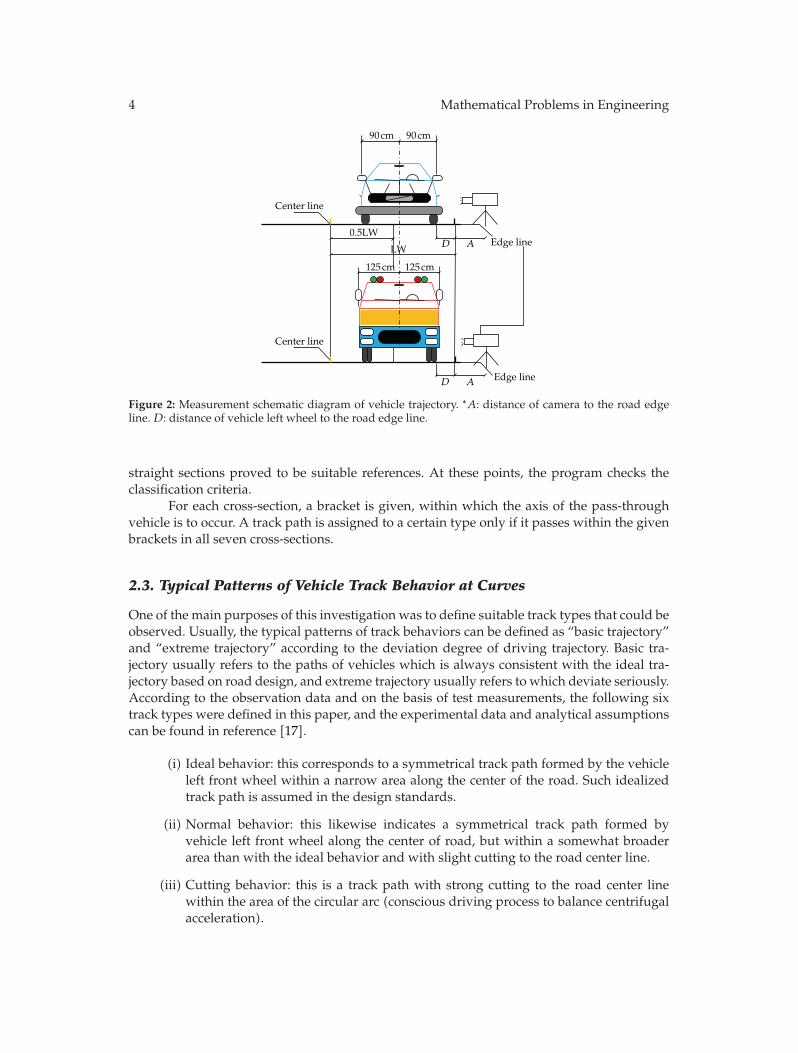
Figure 2 shows the principle at one cross-section. The lane width in the direction ofdriving in the cross-sections at the main curve points and at the limits of the two adjacent


Center line

Center line

LW D A

D A

Edge line

Edge line

90 cm 90 cm

125 cm125 cm

0.5LW

Figure 2: Measurement schematic diagram of vehicle trajectory. ∗A: distance of camera to the road edgeline. D: distance of vehicle left wheel to the road edge line.

straight sections proved to be suitable references. At these points, the program checks theclassification criteria.

For each cross-section, a bracket is given, within which the axis of the pass-throughvehicle is to occur. A track path is assigned to a certain type only if it passes within the givenbrackets in all seven cross-sections.

2.3. Typical Patterns of Vehicle Track Behavior at Curves

One of the main purposes of this investigation was to define suitable track types that could beobserved. Usually, the typical patterns of track behaviors can be defined as “basic trajectory”and “extreme trajectory” according to the deviation degree of driving trajectory. Basic tra-jectory usually refers to the paths of vehicles which is always consistent with the ideal tra-jectory based on road design, and extreme trajectory usually refers to which deviate seriously.According to the observation data and on the basis of test measurements, the following sixtrack types were defined in this paper, and the experimental data and analytical assumptionscan be found in reference [17].

(i) Ideal behavior: this corresponds to a symmetrical track path formed by the vehicleleft front wheel within a narrow area along the center of the road. Such idealizedtrack path is assumed in the design standards.

(ii) Normal behavior: this likewise indicates a symmetrical track path formed byvehicle left front wheel along the center of road, but within a somewhat broaderarea than with the ideal behavior and with slight cutting to the road center line.

(iii) Cutting behavior: this is a track path with strong cutting to the road center linewithin the area of the circular arc (conscious driving process to balance centrifugalacceleration).


Nor

mal

traj

ecto

ry

Idea

l tra

ject

ory

Cut

ting

traj

ecto

ry

Swin

g tr

ajec

tory

Dri

ftin

g tr

ajec

tory

Nor

mal

traj

ecto

ry

Cut

ting

traj

ecto

ry

Swin

g tr

ajec

tory

Dri

ftin

g tr

ajec

tory

Cor

rect

ing

traj

ecto

ry

Cor

rect

ing

traj

ecto

ry

Figure 3: Sketches of track types (example for an up direction).

Table 1: Distribution probability of track types (%) at investigated curves.

(a) (b) (c) (d) (e) (f) (g) (h) (i) (j) (k)P 0.01 0.10 0.11 0.04 0.21 0.12 0.05 0.07 0.09 0.04 0.16

(iv) Drifting behavior: this is asymmetrical track path between the beginning and endof the curve with a pronounced tendency to drive on the down direction at thebeginning of the curve and an increasing drift to the up direction the end of thecurve at left-hand curves, analogous at right-hand curves.

(v) Swinging behavior: this is asymmetrical track path between the beginning and endof the curve with a pronounced tendency to drive on the up direction at the begin-ning of the curve and an increasing drift to the down direction the end of the curveat left-hand curves, analogous at right-hand curves.

(vi) Correcting behavior: this is a track path with increased drifting toward the inside/outside of the curve and subsequent correction of the steering angle in the secondhalf of the curve. It is assumed that this track type is a kind of unconscious drivingbehavior, due to underestimation of the curvature and/or the length of the curve.

Track paths that could not be assigned to those defined types are summarized in aseparate group called “remaining” track paths.

The six paths of the track types described above are illustrated in Figure 3 by the exam-ple of an up direction. And Table 1 gives a distribution probability of the track types permeasurement direction in the curves investigated.

3. Modeling of Driving Trajectory

3.1. Primes Supposition and Modeling Thought

Track path is influenced by many factors in actual. To reveal the formation mechanism ofdriving trajectory and simplify analysis process, assumptions are made as follows:

(i) the study object is dual two-lane road bend section under small volume traffic,which without physical isolation;

(ii) ignore the influence of vertical curve and transverse ultra high, road section is idealhorizontal curve;


O

Edge lineRoad central lineDriving trajectory

Dlat max

Dlat inDver in Dver out

Dlat out

αrrA

Figure 4: Schematic diagram coordinate system of vehicle trajectory.

(iii) suppose ideal bend section is composed by straight-line section and circular curvesection, transition curve is ignored;

(iv) suppose vehicle drives with constant steering angle and speed, vehicle’s longitudi-nal acceleration is ignored;

(v) driver expect to pass the bend section with small curvature, and the steering angleof driving trajectory is the same with that of road circular curve;

(vi) driving trajectory’s deviation from the road centerline satisfies themaximumdevia-tion limitation.

Based on the above assumptions, vehicle driving trajectory while driving on roadcurved section can be expressed by circular curve. To describe vehicle driving trajectoryconveniently, polar coordinate system is constructed as Figure 4. The center of circular curveof road centerline is pole O; horizontal ray passes pole and points to right is polar axis ox;polar angle rotates in counterclockwise direction is positive. In this polar coordinate system,radius of circular curve of road centerline is r, radius of vehicle driving trajectory is rA, radiusof vehicle expected trajectory is rE, and steering angle of road curved section is α.

Under most conditions, the center of vehicle driving trajectory does not coincide withthat of road centerline. To describe driving trajectory conveniently, make the center of vehicledriving trajectory as relative pole to establish polar coordinates of driving trajectory.

Known by actual observation that there are lateral and longitudinal offsets betweenthe endpoints of vehicle driving trajectory and that of road centerline. Longitudinal offsetincludes advance, parallel and lag; lateral offset includes medial offset, lateral offset and zerooffset. The number of cross-point of driving trajectory and road centerline may be 0, 1 or 2.The definition of lateral and longitudinal offsets is as follows:

(1) Dlat max: the maximum lateral offset between driving trajectory and road centerline.

(2) Dlat in: lateral offset between the start point of driving trajectory and that of roadcenterline.

(3) Dlat out: lateral offset between terminal point of driving trajectory and that of roadcenterline.

(4) Dver in: longitudinal offset between start point of driving trajectory and that of roadcenterline.


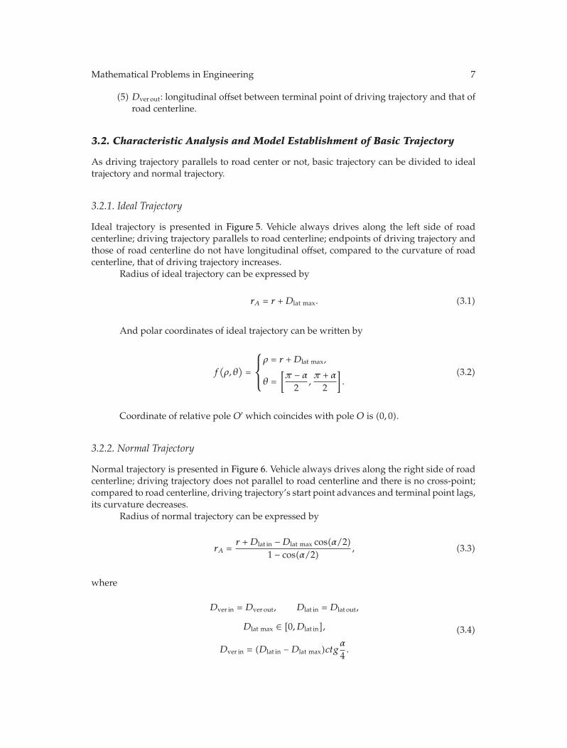
(5) Dver out: longitudinal offset between terminal point of driving trajectory and that ofroad centerline.

3.2. Characteristic Analysis and Model Establishment of Basic Trajectory

As driving trajectory parallels to road center or not, basic trajectory can be divided to idealtrajectory and normal trajectory.

3.2.1. Ideal Trajectory

Ideal trajectory is presented in Figure 5. Vehicle always drives along the left side of roadcenterline; driving trajectory parallels to road centerline; endpoints of driving trajectory andthose of road centerline do not have longitudinal offset, compared to the curvature of roadcenterline, that of driving trajectory increases.

Radius of ideal trajectory can be expressed by

rA = r +Dlat max. (3.1)

And polar coordinates of ideal trajectory can be written by

f(ρ, θ)=

⎧⎪⎨

⎪⎩

ρ = r +Dlat max,

θ =[π − α

2,π + α

2

].

(3.2)

Coordinate of relative pole O′ which coincides with pole O is (0, 0).

3.2.2. Normal Trajectory

Normal trajectory is presented in Figure 6. Vehicle always drives along the right side of roadcenterline; driving trajectory does not parallel to road centerline and there is no cross-point;compared to road centerline, driving trajectory’s start point advances and terminal point lags,its curvature decreases.

Radius of normal trajectory can be expressed by

rA =r +Dlat in −Dlat max cos(α/2)

1 − cos(α/2), (3.3)

where

Dver in = Dver out, Dlat in = Dlat out,

Dlat max ∈ [0,Dlat in],

Dver in = (Dlat in −Dlat max)ctgα

4.

(3.4)


O

Ideal trajectoryr rA


Dlat max

Dlat inDlat out

Figure 5: Characteristic analysis diagram of ideal trajectory.

O Normal trajectory


r

rA

O′

Dlat max

Dlat inDver inDver outDlat out

Figure 6: Characteristic analysis diagram of normal trajectory.

And polar coordinates of normal trajectory can be written by

f(ρ, θ)=

⎧⎪⎪⎪⎨

⎪⎪⎪⎩

ρ = r +Dlat in −Dlat max cos(α/2)

1 − cos(α/2),

θ =[π − α

2,π + α

2

].

(3.5)

Coordinate of relative pole O′ is defined as:

(Dlat max −Dlat in

cos(α/2) − 1,3π2

). (3.6)

3.3. Characteristic Analysis and Model Establishment of Extreme Trajectory

According to driver’s consciousness, extreme trajectory can be divided to conscious extremetrajectory and unconscious extreme trajectory.


Conscious extreme trajectory is the one that driver deliberately chooses to achievesome purposes. At this time, driver has a certain capability and psychological preparation tobear risk. Cutting trajectory is one of the popular conscious extreme trajectories, is the result-ing of driver deliberately deviate road design trajectory, and occupies the opposite directionlane to reduce lateral acceleration or keep high speed. This kind of trajectory usually appearson small radius curved section with small steering angle.

Unconscious extreme trajectory is the resulting as driver underestimates the curvatureof road curved section and chooses this trajectory unconsciously. While driver discoveredthe trend to this trajectory, the general response is to turn abruptly to correct vehicle drivingtrajectory. Swinging and drifting trajectories are the popular ones of unconscious extremetrajectories. Although driver’s purpose is to reduce vehicle’s lateral acceleration, but largeamount of survey found that the two trajectories will lead to lateral acceleration’s suddenincreases in partial part. High driving speed and braking operation are apt to cause vehicleout of control.

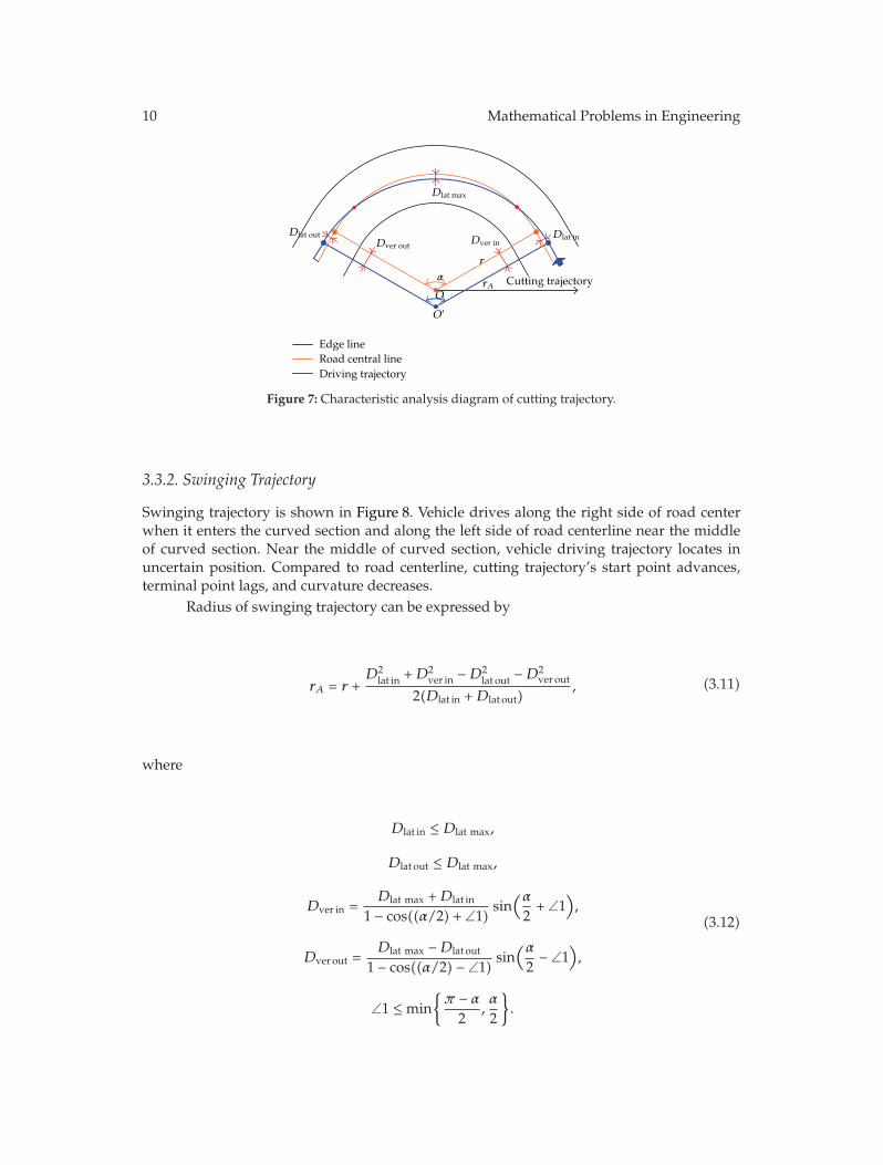
3.3.1. Cutting Trajectory

Cutting trajectory is presented in Figure 7. Vehicle drives along the right side of road centerwhen it enters and pulls out the curved section, drives along the left side of road centerlinenear the middle of curved section. Compared to road centerline, cutting trajectory’s startpoint advances, terminal point lags, and curvature decreases.

Radius of cutting trajectory can be expressed by

rA = r +Dlat max · cos(α/2) +Dlat in

1 − cos(α/2), (3.7)

where

Dlat in ∈ [0,Dlat max],

Dver in = (Dlat max +Dlat in)ctgα

4.

(3.8)

And coordinate of cutting trajectory can be written by

f(ρ, θ)=

⎧⎪⎪⎪⎨

⎪⎪⎪⎩

ρ = r +Dlat max · cos(α/2) +Dlat in

1 − cos(α/2),

θ =[π − α

2,π + α

2

].

(3.9)

Coordinate of relative pole O′ is defined as

(Dlat max +Dlat in

1 − cos(α/2),3π2

). (3.10)


Cutting trajectoryO


r

rA

O′

α

Dlat max

Dlat inDver inDver out

Dlat out

Figure 7: Characteristic analysis diagram of cutting trajectory.

3.3.2. Swinging Trajectory

Swinging trajectory is shown in Figure 8. Vehicle drives along the right side of road centerwhen it enters the curved section and along the left side of road centerline near the middleof curved section. Near the middle of curved section, vehicle driving trajectory locates inuncertain position. Compared to road centerline, cutting trajectory’s start point advances,terminal point lags, and curvature decreases.

Radius of swinging trajectory can be expressed by

rA = r +D2

lat in +D2ver in −D2

lat out −D2ver out

2(Dlat in +Dlat out), (3.11)

where

Dlat in ≤ Dlat max,

Dlat out ≤ Dlat max,

Dver in =Dlat max +Dlat in

1 − cos((α/2) + ∠1)sin(α2+ ∠1

),

Dver out =Dlat max −Dlat out

1 − cos((α/2) − ∠1)sin(α2− ∠1

),

∠1 ≤ min{π − α

2,α

2

}.

(3.12)


Swinging trajectoryO


r

rA

O′∠1

Dlat max

Dlat in

Dver inDver out

Dlat out

Figure 8: Characteristic analysis diagram of swinging trajectory.

And polar coordinates of swinging trajectory can be written by

f(ρ, θ)=

⎧⎪⎪⎪⎪⎨

⎪⎪⎪⎪⎩

ρ = r +D2

lat in +D2ver in −D2


2(Dlat in +Dlat out),

θ =[π − α

2,π + α

2

].

(3.13)


(Dver in

sin((α/2) + ∠1),3π2

+ α

). (3.14)

3.3.3. Drifting Trajectory

Drifting trajectory is shown in Figure 9. Vehicle drives along the left side of road centerwhen it enters the curved section and along the right side of road centerline near the middleof curved section. Near the middle of curved section, vehicle driving trajectory locates inuncertain position. Compared to road centerline, curvature of drifting trajectory decreases.

Radius of drifting trajectory can be expressed by

rA = r +D2

ver in −D2lat in +D2


2(Dver in +Dlat out), (3.15)


Drifting trajectoryO


r

rA

O′ ∠1

Dlat max

Dlat inDver in

Dver out

Dlat out

Figure 9: Characteristic analysis diagram of drifting trajectory.

where

Dlat in ≤ Dlat max,

Dlat out ≤ Dlat max,

Dver in =Dlat in −Dlat max

cos((α/2) − ∠1) − 1sin(α2− ∠1

),

Dver out =Dlat max +Dlat out

1 − cos((α/2) + ∠1)sin(α2+ ∠1

),

∠1 ≤ min{π − α

2,α

2

}.

(3.16)

And polar coordinates of drifting trajectory can be written by

f(ρ, θ)=

⎧⎪⎪⎪⎪⎨

⎪⎪⎪⎪⎩

ρ = r +D2

ver in −D2lat in +D2


2(Dver in +Dlat out),

θ =[π − α

2,π + α

2

].

(3.17)


(Dlat in −Dlat max

cos((α/2) − ∠1) − 1,3π2

− α

). (3.18)

3.3.4. Correcting Trajectory

Correcting trajectory is shown in Figure 10. Vehicle drives near the road centerline when itenters and pulls out the curved section. There are no cross-point between driving trajectory


Correcting trajectory

O


r

rA

O′

Dlat max

Dlat in

Dver inDver out

Dlat out

Figure 10: Characteristic analysis diagram of correcting trajectory.

and road centerline. Compared to road centerline, correcting trajectory’s start point lags andterminal point advances, and curvature increases.

Radius of correcting trajectory can be expressed by

rA = r − Dlat max cos(α/2) −Dlat in

1 − cos(α/2), (3.19)

where

Dver in =Dlat max −Dlat in

1 − cos(α/2)sin

α

2. (3.20)

And polar coordinates of correcting trajectory can be written by:

f(ρ, θ)=

⎧⎪⎪⎪⎨

⎪⎪⎪⎩

ρ = r − Dlat max cos(α/2) −Dlat in

1 − cos(α/2),

θ =[π − α

2,π + α

2

].

(3.21)


(Dlat max −Dlat in

1 − cos(α/2),π

2

). (3.22)

4. Simulation and Verification

The six developed models are applied to simulate driving track behaviors at curves in orderto study its rationality. The simulation diagrams with different corner (120◦ and 60◦) can beshown in Figures 11 and 12 the parameters in models are varied between limits except radius.It can be seen that the models are verified by digital simulation results.


(a) Ideal trajectory (b) Normal trajectory

(c) Cutting trajectory (d) Correcting trajectory

(e) Drifting trajectory (f) Swinging trajectory

Figure 11: Simulated diagram with the corner angel being 120◦.

5. Optimized Trajectory and Vehicle Yaw Stability

2-degree-of-freedom vehicle dynamic model is used to analyze vehicle yaw rate under differ-ent driving trajectories, which is presented as follows:

mV(β + r

)= −2kf

(

β +lf

Vr − δ

)

− 2kr(β − lr

Vr

),

Izr = −2kf(

β +lf

Vr − δ

)

lf + 2kr(β − lr

Vr

)lr ,

(5.1)

where m is vehicle total mass, V is driving speed, β is sideslip angle, r is yaw rate. kf , kr arefront and rear tires’ cornering stiffness, respectively. lf , lr are front and rear track, respectively.δ is steer angle. Iz is yaw moment of inertia of total mass.

Matlab is used to simulate vehicle time varying characteristics numerically. Vehicleyaw rates under normal and ideal trajectory are presented in Figure 13.

As seen from Figure 13, vehicle yaw rate under normal trajectory is 11.11% smallerthan that under ideal trajectory, which indicates vehicle steering stability under normaltrajectory is better than that under ideal trajectory.


0

4

8

12

16

20

−40 −20 −10−30 0 10 3020 40

(a) Ideal trajectory

0

4

8

12

16

20

−40 −20 −10−30 0 10 3020 40

(b) Normal trajectory

0

4

8

12

16

20

−40 −20 −10−30 0 10 3020 40

(c) Cutting trajectory

0

4

8

12

16

20

−40 −20 −10−30 0 10 3020 40

(d) Correcting trajectory

0

4

8

12

16

20

−40 −20 −10−30 0 10 3020 40

(e) Drifting trajectory

0

4

8

12

16

20

−40 −20 −10−30 0 10 3020 40

(f) Swinging trajectory

Figure 12: Simulated diagram with the corner angel being 60◦.

Vehicle yaw rates under four kinds of extreme trajectories are presented in Figure 14.As seen from Figure 14, yaw rate under swing trajectory is the biggest and yaw rate undercutting trajectory is the smallest, which indicates that vehicle has the best steering stabilityunder cutting trajectories while it has the worst steering stability under swing trajectory.

According to the analysis above, compared to other driving trajectories, normal andcutting trajectory are the safer driving trajectories for vehicle passing by the curves.

6. Conclusions

In contrast to the usual descriptions of driving behavior in curve areas in terms of speeds,this paper investigated track behavior. To this point, a classification of the driving processesaccording to the type of the track paths along curves was developed and the trajectorymodelswere established, respectively, combining with curve geometry of two-way highway road. Atlast, 2-degree-of-freedom vehicle dynamic model was used to analyze vehicle yaw rate underdifferent type of trajectories, considering the sight distance, normal trajectory and cuttingtrajectory were determined as the optimum driving trajectories. The study findings havegreat importance to providing theoretical support and developing suitable countermeasuresto the reasonable optimization of widen curves, design of alignment, and the management ofcounter flow conflicts.


0 0.2 0.4 0.6 0.8 1 1.2 1.4 1.6 1.8 20

0.020.040.060.080.1

0.120.140.160.180.2

Time (s)

Yaw

rat

e (r

ad/

s)

Normal trajectoryIdeal trajectory

Figure 13: Vehicle yaw rates under two kinds of basic trajectory.

0 0.2 0.4 0.6 0.8 1 1.2 1.4 1.6 1.8 20

0.020.040.060.080.1

0.120.140.160.180.2

Time (s)

Yaw

rat

e (r

ad/

s)

Cutting trajectoryCorrecting trajectory

Drifting trajectorySwing trajectory

Figure 14: Vehicle yaw rates under four kinds of extreme trajectories.

Since we ignored the transition curves in deriving the vehicle track models forsimplification purpose, thus, what the vehicle track models really are when the transitioncurves are considered will be conducted in a future study.

Acknowledgment

This study is supported by the National Natural Science Foundation of China (nos. 50978114and 51208225).

References

[1] S. G. Charlton and J. J. D. Pont, “Curved speed management,” Research Report 323, Land TransportNew Zealand, Wellington, New Zealand, 2007.

[2] Arbeitsgruppe Verkehrssicherheit (AGVS) and Federal Traffic Safety Working Group, Traffic Safety byNight, Traffic- Engineering- Related Improvements to the Highway Infrastructure, EJPD, Berne, Switzerland,1980.


[3] J. C. Glennon and G. D. Weaver, “The relationship of vehicle paths to highway curve design,”Research Report 134-6, Texas Highway Department and the Federal Highway Administration, 1971.

[4] S. Xiao-Duan and T. Dean, “Impact of edge lines on safety of rural two-lane highways,” Tech. Rep.414, Civil Engineering Department University of Louisiana at Lafayette, Lafayette, La, USA, 2005.

[5] U. Scheifele and P. Spacek,Measuring Poles: A Measuring Device for Surveying Driving Behavior on High-ways, IVT-ETH Zurich and Planitronic Zurich, supported by the Swiss Road Safety Fund, Zurich,Switzerland, 1992.

[6] P. Spacek, “Driving behavior and accident occurrence in curves, driving behavior in curve areas,”Research Project 16/84, IVT-ETH, Swiss Federal Highways Office, Zurich, Switzerland, 1998.

[7] P. Spacek, Environmental Impact of Traffic, Section: Road Safety of Traffic Facilities, Lecture Notes, IVT-ETH, Zurich, Switzerland, 2003.

[8] P. Spacek, “Track behavior in curve areas: attempt at typology,” Journal of Transportation Engineering,vol. 131, no. 9, pp. 669–676, 2005.

[9] Federal Highway Administration, Development of a Driver Vehicle Module for the Interactive HighwaySafety Design Model, United States Department of Transportation, Washington, DC, USA, 2007.

[10] M. Althoff, O. Stursberg, and M. Buss, “Safety assessment of driving behavior in multi-lane trafficfor autonomous vehicles,” in Proceedings of the IEEE Intelligent Vehicles Symposium, pp. 893–900, June2009.

[11] X. Guan, Z. Gao, and K. Guo, “Driver fuzzy decision model of vehicle preview course and simulationunder typical road conditions,” Automotive Engineering, vol. 23, no. 1, pp. 13–20, 2001 (Chinese).

[12] G. Zhen-Hai, G. Xin, and G. Kong-Hui, “Driver fuzzy decision model of vehicle preview course,”Natureal Science Journal of Jilin University of Technology, vol. 30, no. 1, pp. 7–10, 2000 (Chinese).

[13] P. Xiao-Dong, D. Zhi-Gang, J. Hong et al., “Experiment research on relationship between the variationof drivers’ heart rate and systolic blood pressure and a lignment of mountainous highway,” ChineseJournal of Ergonomics, vol. 12, no. 2, pp. 16–18, 2006 (Chinese).

[14] W. H. Wang, C. X. Ding, G. D. Feng, and X. B. Jiang, “Simulation modelling of longitudinal safetyspacing in inter-vehicles dynamics interactions,” Journal of Beijing Institute of Technology, vol. 19, sup-plement 2, pp. 55–60, 2010.

[15] W. Wang, Y. Mao, J. Jin et al., “Driver’s various information process and multi-ruled decision-making mechanism: A fundamental of intelligent driving shaping model,” International Journal ofComputational Intelligence Systems, vol. 4, no. 3, pp. 297–305, 2011.

[16] W.Wuhong, G. Weiwei, M. Yan et al., “Model-based simulation of driver expectation in mountainousroad using various control strategies,” International Journal of Computational Intelligence Systems, vol. 4,no. 3, pp. 1187–1194, 2011.

[17] R. Yuan-Yuan, L. Xian-Sheng, R. You, G. Rachel, and G. Wei-Wei, “Study on driving dangerous areain road curved section based on vehicle track characteristics,” International Journal of ComputationalIntelligence Systems, vol. 4, no. 6, pp. 1237–1245, 2011.

Submit your manuscripts athttp://www.hindawi.com

Hindawi Publishing Corporationhttp://www.hindawi.com Volume 2014

MathematicsJournal of


Mathematical Problems in Engineering

Hindawi Publishing Corporationhttp://www.hindawi.com

Differential EquationsInternational Journal of

Volume 2014

Applied MathematicsJournal of


Probability and StatisticsHindawi Publishing Corporationhttp://www.hindawi.com Volume 2014

Journal of


Mathematical PhysicsAdvances in

Complex AnalysisJournal of


OptimizationJournal of


CombinatoricsHindawi Publishing Corporationhttp://www.hindawi.com Volume 2014

International Journal of


Operations ResearchAdvances in

Journal of


Function Spaces

Abstract and Applied AnalysisHindawi Publishing Corporationhttp://www.hindawi.com Volume 2014

International Journal of Mathematics and Mathematical Sciences


The Scientific World JournalHindawi Publishing Corporation http://www.hindawi.com Volume 2014


Algebra

Discrete Dynamics in Nature and Society



Decision SciencesAdvances in

Discrete MathematicsJournal of

Hindawi Publishing Corporationhttp://www.hindawi.com

Volume 2014 Hindawi Publishing Corporationhttp://www.hindawi.com Volume 2014

Stochastic AnalysisInternational Journal of

Documents

Study on Vehicle Track Model in Road Curved Section Based