Embed Size (px)
Citation preview

International Scientific Conference eRA-8
ISSN-1791-1133 1
Study of the response of open CR-39 detector to
radon and progeny by Monte Carlo simulation with
SRIM 2013.
D. Nikolopoulos1
, E. Vlamakis1
, N. Chatzisavvas1
, P. H.Yannakopoulos1
, X.
Argyriou1
, E. Petraki1,2
, S. Kottou3
, T. Sevvos1
, N. Temenos1
, Y. Chaldeos1
, S.
Filtisakos1
, N. Gorgolis1
, S. Potozi4
, D. Koulogliotis1
, A. Zisos5
1
Department of Computer Electronic Engineering, TEI of Piraeus, Greece 2Department of Engineering and Design, Brunel University, London, UK.
3
Medical Physics Department, Medical School, University of Athens, Greece 4
Department of Environmental Technology and Ecology, TEI of Ionian Islands, GreeceTEI of Piraeus, Greece
ABSTRACT :
Special GNU gcc Monte Carlo codes were developed for the calculation of the sensitivity of bare CR39 detectors to alpha particles emitted by radon and progeny. The codes were designed so as to utilise the latest SRIM2013 outputs in optimal way. Several malcontent output of SRIM 2013 was corrected. The codes employed all existing model data regarding CR-39's internal sensitivity dependence on critical angle and etching time. Monte Carlo outputs were discriminated based on the initial energy of the incident alpha particles. The codes accounted the energy influence due to the attenuation of the overlying air layer. Latent track formation and corresponding differentiation due to etching process were, however, not taken into account. Code input can be adapted easily for different ambient concentrations of radon and progeny, i.e., for different values of equilibrium factor. Results showed excellent consistency with the limited published outcomes.
1. INTRODUCTION
Solid State Nuclear Track Detectors (SSNTDs) are widely used in science and technology. One of the best competitors for detecting alpha particles, emitted by radon and progeny, is CR-39. Due to its detection properties, CR-39 SSNTD has been widely employed in radon measurements worldwide. CR-39's suitable depth of chemical etching is the depth that varying track density has any particles

International Scientific Conference eRA-8
ISSN-1791-1133 2
fluctuates and rapid loss. During the last decade, numerous investigations have been published on utilising CR-39 SSNTDs in long-term radon progeny measurements. Various such theoretical methods, based on more or less accurate models, have been proposed in the past (Nakahara et al., 1980; Akber et al., 1980; Abu-Jarad et al., 1980; Somogyi et al., 1984; Damkjaer, 1986; Urban, 1986; Kleis et al., 1991; Qureshi et al., 1991; Nikezic et al., 1992, 1995; Andriamanantena and Enge, 1995; Sima, 1995; Andriamanantena et al., 1997; Djeal et al., 1997; Nikezic and Yu, 1998; Amgarou et al. 2006; Eappen et al 2012 ; Stallic and Nikezic 2012). Although the related results are promising, up-to date, a standard methodology still not exists. Some related papers include also Monte Carlo modeling, especially in conjunction with special software. Sima (1995) developed software for the realistic calculation of the sensitivity of various etched track radon monitors. In calculations, typical observation criteria were included. Nikezic et al. (1995) developed another software which simulated a-particle detection of CR 39 detectors. Through this program and its modifications (Yu et al., 2003), the dependence of CR-39's detection efficiency was determined as a function of etching time and Vb bulk etch rate. Despite the scientific work in this subject area (e.g. Kappel et al., 1997; Nikezic and Yu, 2000; Rehman e al., 2003; Rickards et al., 2013), it is still an open issue to determine accurately alpha energy and angle distributions at the surface of open CR-39 solid state nuclear track detectors due to decay of radon and progeny. Most important is the estimation of a realistic calibration factor of bare CR-39 SSNTDs. One of the major disadvantages of such simulations up-to-date is that all approaches included the energy calculating code of every particle. This increases simulation time significantly. To reduce simulation time, the energy of the alpha particles as a function of the distance traveled in CR-39 was recently introduced as an alternative (Rezaie and Nejad, 2012; Rezaie et al., 2013).
Noticeable is the effort in employing special software for the calculation of the interactions of ions with matter prior to calculating the alpha efficiency of SSNTDs (e.g. Sharma, A et al 2000;Rehman FU et al 2003). Among others, SRIM (Stopping and Range of Ions in Matter) is a group of programs which may calculate all interactions of ions with matter and for this reason has attracted attention. The core of SRIM is a program called Transport of ions in matter (TRIM). SRIM and TRIM were developed by James F. Ziegler and Jochen P. Biersack about 1983 and they are continuously upgraded with the great changes that took place every five years. SRIM is based on a Monte Carlo simulation method. Input parameters are the type of ion and its initial energy in the range of 10 eV to 2 GeV and the target material being considered either s single-or multi- layered. SRIM output includes lists and diagrams. The programs were developed so they can be interrupted any time and resume later with a convenient GUI. These characteristics make SRIM very practical. Nevertheless, SRIM does not include dynamic changes of synthesis in materials. This limits somehow its usefulness. Significant however issues include threshold displacement energy as a step function for each element and layer design of target systems. Nevertheless, simulation of materials with composition differences in 2D or 3D is not possible (Sharma, A et al 2000;Dwivedi K et al 2001). Using SRIM 2008 software, alpha range and stopping power data was easily extracted and the data can be used reliably.

International Scientific Conference eRA-8
ISSN-1791-1133 3
The present paper focused on modelling the response of bare CR-39 detectors to alpha -particles emitted by radon and progeny through Monte Carlo Methods and the use of the latest version SRIM2013..Beforehand, theoretical and experimental CR-39 efficiency factors were calculated for alpha-particles emitted by radon and progeny in air. The scope, was to determine the efficiency of bare CR-39 SSNTDs for a combined use of bare CR-39 and cup-type dosimeters in radon measurements.
2. MATERIALS AND METHODS
2.1 Calculation of Alpha Energy versus Distance
If an alpha-particle of energy E1 is emitted within an effective distance, l , from the surface of a CR-39 detector, then it will hit the detector with energy E2 due to interactions with molecules of the surrounding medium. The distance l must be smaller or equal than the range of alpha particles in the medium. The distance l is equal to the difference between range R1 of the alpha particle of energy E1 and
R2 of the particle of energy E2 (Nikezić et al 2000; DPaul H 2006) l=R
1− R
2 (1)
If the alpha-particle is generated through a decay scheme and E1 is its initial energy, then all possible distance values l from CR-39's surface will be
l=Rmax
− R (2)
where Rmax is the corresponding maximum range and R is the range corresponding to a hit-energy E .
To properly define l , all range data of alpha particles' energies between 0.5-10 MeV were extracted from SRIM2013 output tables after properly adjusting for several baffling characters. The range data were then fitted to the non-linear equation (3), considering absence of straggling (Rezaie et al 2012):
R=a⋅E+b⋅E2
+c⋅E3
(3)
By replacing R from (3) in (2), then the distance l versus alpha energy can be
obtained:
l=Rmax−(a⋅E +b⋅E2
+c⋅E3
) (4)
Inversely, the energy of alpha particles at a distance l from the point of emission
were calculated by the reciprocal of equation (3).
2.2 Monte Carlo simulation
For the Monte-Carlo simulation, the actual dimensions of the CR-39 detectors employed in radon and progeny measurements within the framework of the

International Scientific Conference eRA-8
ISSN-1791-1133 4
NRSF ―Thalis‖ Project of the Technological Education Institute of Piraeus were
employed, namely of 1×1 cm2
surface area and 0.5 mm thickness. CR-39's surface was put on the x-y plane. Since alpha-particles originating from radon
and progeny may have different initial energies (222
Rn 5.49 MeV, 218
Po 6.00 MeV, 214
Po 7.68 MeV), a surface area was considered vertical to the z-axis, with dimensions (1+2⋅R)×(1+2⋅R) (Sima 1995), where R was taken equal to the
corresponding alpha-particle range (4.09 cm for alphas of 222
Rn, 4.67 cm for
alphas of 218
Po and 6.78 cm for alphas of 214
Po) (Nikezic, 1994). The effective volume around CR-39 (Fig.1) was then calculated by equation (5) (Sima 1995):
V =R×(1+2⋅R)×(1+2⋅R) (5)
Outside the effective volume, alpha-particles do not reach CR-39's surface since the distance traveled is larger than the alpha range. Only alpha-particles generated within volume V are detectable. For the simulation, inside the effective volume, a random point P1 (X1, Y1, Z1) was computationally created. At this point, an alpha particle from radon's decay was considered to be emitted with random cylindrical angles θ ,φ .
Depending on the emission angles, a hit-state was calculated, namely being 1 if the alpha could hit CR-39's surface and 0, otherwise. For an alpha-particle of hit-state 1, the hit-angles θh ,φh to the XY entrance surface of CR-39 were calculated from the cartesian coordinates of point P1, the angles θ ,φ and the dimensions of CR-39. Since CR-39 does not register alpha-particles with hit-angles above a critical angle, θcr , the alpha-particle was accepted and processed further only if θh≤θcr , otherwise it was rejected. An accepted alpha-particle could be registered, and if so, the distance l traveled in CR-39's surrounding medium was calculated again from the cartesian coordinates of P1, the hit-angles and CR-39's dimensions. From l ,θh ,φh data, the arrival point P2 (X2,Y2,Z2) in respect to the detector's plane was calculated thereafter. In parallel, the hit-energy Eh was calculated from the output SRIM2013 for the distance l according to equation (4). Having calculated hit-data Eh ,θ h,φh for an accepted alpha-particle, the distance, d , traveled inside CR-39 was finally calculated from SRIM2013 output. Iterating the above procedure, the energy-angle distribution of various radon's decay alpha-particle showers was also calculated.
Fig.1: Effective volume for CR-39 for alpha-particles emitted due to decay of radon and
progeny. R is the corresponding range, namely 4.09 cm for alphas of 222
Rn with initial energy of
5.49 MeV, 4.67 cm for alphas of 218
Po with initial energy of 6.00 MeV and 6.78 cm for alphas of 214
Po with initial energy of 7.68 MeV.

International Scientific Conference eRA-8
ISSN-1791-1133 5
Figure 2 presents the flow-diagram of the Monte Carlo simulation
Fig.2: Flowchart of Monte Carlo simulation of alpha particles of radon's decay traveling around
and within CR-39 detectors.
3. RESULTS
The range-energy dependence of equation (4) was found equal to:
R=3.34773⋅E+0.34937⋅E2
+0.02142⋅E3
(6) Employing (6) in (4) the
distance-energy dependence was calculated as l=Rmax−(3.34773⋅E
+0.34937⋅E 2
+0.02142⋅E3
) (7) where Rmax =4.09 cm for alpha-particles
originating from 222
Rn, Rmax =4.67 cm for alpha-particles originating
from 218
Po and Rmax =6.78 cm for alpha-particles originating from 214
Po. The reciprocal of equation (7) yielded the calculation of the energy-distance dependence as presented in Table 1.
Table 1: Relation of energy of alpha particles versus distance traveled in (a) CR-39 and (b) air.
Radon and Progeny CR-39 E(MeV), d (μm)
222Rn E=5.49-0.10148 . d - 0.000589. d 2
218Po E=6-0.10054 . d + 0.000004332 d 2
214Po E=7.69-0.09899 . d + 0.000798 d 2
Air E(MeV) , l (mm)
222Rn E=5.49-0.081 . l l- 0.0009333 . l2
218Po E=6-0.07312 . l - 0.00075 . l2
214Po E=7.69-0.05612 . l - 0.000024 . l2
Generating equal number of alpha-particles originating from 222
Rn, 218
Po and 214
Po, calculating however the Monte Carlo parameters independently for each

International Scientific Conference eRA-8
ISSN-1791-1133 6
radionuclide, the sensitivity of each nuclide was calculed assuming steady-state between radon and progeny in accordance to the Jacobi's model (Nazarrof and
Nero 1988). According to this model the concentrations of 218
Po and 214
Po were calculated by presumed concentration of radon employing a constant value for the equilibrium factor (Nazarrof and Nero 1988). The number of alpha particles recorded per day within the effective volume of CR-39 calculated according to
the Jacobi's model was Nj =0.5×86400×C×F × R×(1+2 R˙)×(1+2 R
˙) (8) where C
represents the presumed value of the radon concentration, F is the mean equilibrium factor and R is the corresponding range of equations (5) and (7),
namely R= Rmax, j for each one of 222
Rn, 218
Po and 214
Po. Constant 86400 (s per day) transforms Becquerels to dimensionless units. It is an interesting finding, that a coefficient of 0.5 was calculated in equation (8). This important finding implies that half of the alpha particles emitted were issued forward to CR-39 and the remaining half, backwards. Transmitted alpha particles from CR-39 were found to be negligible. This may be attributed to the fact that alpha particles have low curvature paths (Llerena et al., 2011;, Martins et al., 2013; Cosma et al.,
2013). CR-39 sensitivity coefficient was found equal to 4.6 (tracks /cm2
) per
kBq⋅m−3
⋅h .
Fig.3 presents the calculated alpha energy spectrum at the surface of CR-39 of
dimensions of 1×1 cm2
dueto 1 1 kBq⋅m−3
activity of radon and a mean equilibrium factor of 0.4.
Fig.3: Alpha energy spectrum of radon and progeny calculated for 1 1 kBq⋅m−3
activity of radon
and a mean equilibrium factor of 0.4
Table 2 presents simulation results of the association of the penetration depths versus the incidence angles of alpha-particles in CR-39 due to radon and
progeny. Most penetrating are the 218
Po alpha-particles that hit CR-39 with angles
less between 300
and 500
with penetrating depths between 51 μm and 55 μm .
Angles between 300
and 500
are associated with maximum penetrating depths
also for alpha-particles due to 222
Rn and 214
Pb decay. Alpha-particles due to
decay of 222
Rn do not hit CR-39 within 500
and 750
whereas those of 214
Po in the

International Scientific Conference eRA-8
ISSN-1791-1133 7
range 500
and 700
. Hence alpha-particle that hit CR-39 between 500
and 700
will
be due to 218
Po's decay and will create tracks between 14 μm and 45 μm . According to Table 2, observed tracks in the depth of 7 μm and 12 μm are due to 214
Po's alpha-particles incident with angles between 100
and 400
. Observed tracks
at depths between of 32 μm and 52 μm are related to 218
Po's alpha-particles
incident between 00
and 50
. Tracks between 42 μm and 49 μm are related to
decay of 222
Rn and alpha-particles incident between 300
and 500
. Tracks between
49 μm and 55 μm are definitely related to 214
Po's alpha-particles incident between
350
and 560
. According to Table 2, all alpha-particles emitted due to radon's decay and registered in CR-39, finalise their path at the depth of 55 μm .
Table 2. Relation between incident angles and penetration depths in CR-39 for alpha-particles
originating due to decay of radon and progeny.
222Rn
Angle (degrees) 2-18 20-30 30-50 75-80
Depth (μm) 25-30 30-38 42-49 28-42
218Po
Angle (degrees) 3-30 30-60 30-50 50-70
Depth (μm) 32-52 25-35 51-55 14-45
214Po
Angle (degrees) 0-5 25-55 30-50 70-75
Depth (μm) 7-12 18-25 49-51 24-44
4. CONCLUSIONS
This paper reported a newly developed Monte-Carlo simulation for the calculation of the efficiency of bare CR-39 detectors. Simulation combined Monte-Carlo techniques, experimental data and the latest version of SRIM (SRIM2013). The sensitivity coefficients of CR-39 for radon and progeny were calculated independently for each nuclide. CR-39 sensitivity coefficient was found equal to
4.6 (tracks /cm2
) per kBq⋅m−3
⋅h assuming the Jacobi's steady-sate model. Additional modelling rendered calculation of CR-39's energy and angular distributions of alpha-particles due to radon and progeny.
5. ACKNOWLEDGMENT
This work has been co-financed by Greece and the European Union, under the European Social Fund NSRF 2007-2013 (Thales). Managing Authority: Greek Ministry of Education and Religious Affairs, Culture and Sports.

International Scientific Conference eRA-8
ISSN-1791-1133 8
REFERENCES
Aljarrah I.A., O.D. Al-Khaleel, H.M. Al-Khateeb , K.M. Aljarrah , 2012, F.Y. Alzoubi. A new
method for measuring tracks density in CR-39 detectors by compensating for overlapping
tracks , Radiat. Meas. Vol 47, 537-540 .
Balestra S., Cozzi, M., Giacomelli, G., Giacomelli, C., Giorgini, M., Kumar, A.,Mandrioli, G.,
Manzoor, S., Margiotta, A.R., Medinaceli, E., Patrizii, L., Popa, V.,Qureshi, I.E., Rana, M.A.,
Sirri, G., Spurio, M., Togo, V., Valieri, C., Bulk etch rate measurements and calibrations of
plastic nuclear track detectors., 2007, Nuclear Instruments and Methods in Physics
Research, B 254, 254-258.
Banjanac R, Dragić A, Grabež B, Joković D, Markushev D, Panić B, et al., 2006, Indoor Radon
measurements by nuclear track detectors: Applications in secondary schools. Facta
universitatis-series: Physics, Chemistry and Technology., 4(1): 93-100.
Bavarnegin E., N. Fathabadi , M. Vahabi Moghaddam , M. Vasheghani Farahani , M. Moradi, A.
Babakhni., 2013, Radon exhalation rate and natural radionuclide content in building
materials of high background areas of Ramsar, Iran, Journal of Environmental Radioactivity
117 (2013) 36-40.
Bianco S.J. Computer Physics Research Trends: Nova Science Publishers; 2007.
Brown J.M.C., McKean, N., Solomon, S., Tinker, R.A., 2006, Development of a Semi-Automated
Nuclear Track Etch Counting System for CR-39_ Radon Plaques.In: Proceedings of the 9th
South Pacific Environmental Radioactivity Association Conference, SPERA.
Chekirine M., Ammi, H., 1999, Stopping power of 1.0e3.0 MeV helium in Mylar, Radiat. Measur.
Vol 30., 131-135 .
Chen J., D. Moir, A. Sorimachi, S. Tokonami, 2011, Assessment of radon equilibrium factor from
distribution parameters of simultaneous radon and radon progeny measurements, Radiation
and Environmental Biophysics Vol 50 (4) 85.
Constantin C. , Alexandra Cucos¸ Dinu , Botond Papp , Robert Begy, 2013, Carlos Sainz.Soil and
building material as main sources of indoor radon in Bait¸a-Stei radon prone area (Romania),
Journal of Environmental Radioactivity 116, 174 179.
Doi M., Fujimoto, K., Kobayashi, S., Yonehara, H., 1994, Spatial distribution of thoron and radon
concentrations in the indoor air of traditional Japanese wooden house. Health Physics, Vol
66 (1), 43-49.
Durrani S.A., Ilic, R., 1997, Radon Measurements by Etched Track Detectors .
Durrami. S. A. Hie. R., Applications in Radiation Protection, Earth Sciences and the
Environment., 1997 Pergamon Press, Oxford.
Dwivedi K.K., Mishra, R., Tripathy, S.P., Kulshreshtha, A., Sinha, D., Srivastava, A.,Deka, P.,
Bhattacharjee, B., Ramachandran, T.V., 2001, Nambi, K.S.V., Simultaneous determination
of radon, thoron and their progeny in dwellings. Radiation Measurements Vol 33, 7-11.
Eappen K.P., Mayya, Y.S., 2004, Calibration factors for LR-115 (type-II) based radon thoron
discriminating dosimeter. Radiation Measurements Vol 38, 5-17.
Environmental Protection Agency, 1999, National Primary Drinking Water Regulations Radon-

International Scientific Conference eRA-8
ISSN-1791-1133 9
222. Proposed Rule. Federal Register 2 64 (211): 5924559294.
Geiger H., Marsden E., 1909, On a Diffuse Reflection of the α-Particles. Proceedings of the Royal
Society of London Series A, Containing Papers of a Mathematical and Physical Character.
495-500.
Henshaw D., Fews A, Keitsch P, Wilding R, Close J, Heather N, et al., 2001, Atmospheric
washout of Radon shortlived daughters: implications for the radiation dose to the skin. 12th
UK Aerosol Conf. Bath, UK.
Iacob O., Grecea C, Capitanu O, Rascanu V, Agheorghiesei D, Botezatu E, et al., 2001,
Population exposure to indoor Radon and thoron progeny. Population. Vol 9(1):5-12.
Jafarizadeh, M. Taheri, N. Rastkhah, M.R. Kardan, 2010, Measurements of radon level in two
tourist caves in Iran, in: Proceedings of European Conference on Individual Monitoring of
Ionizing Radiation, Athens, Greece.
Kappel R., Keller G, Nickels R, Leiner U., 1997, Monte Carlo computation of the calibration factor
for 222Rn measurements with electrochemically etched polycarbonate nuclear track
detectors. Radiation protection dosimetry. 71(4) 261 267.
Kazuki I., Masahiro Hosoda, Hiroyuki Tabe, Tetsuo Ishikawa, Shinji Tokonami, and Hidenori
Yonehara, 2013, Activity Concentrations of Natural Adionuclides and Radon and Thoron
exhalation Rates in Rocks used as Decorative Wall Coverings in Japan, Health Physics
Society.
Kendall GM, Smith TJ., 2002, Doses to organs and tissues from Radon and its decay products.
Journal of Radiological Protection. 22(4):389-406.
Khan RFH, Ahmad N., 2001, Studying the response of CR-39 detectors using the Monte Carlo
technique. Radiation Measurements. Vol 33(1):129-37.
Khateeb Al., H.M., Al-Qudah, A.A., Alzoubi, F.Y., Alqadi, M.K., Aljarrah, K.M., 2012, Radon
concentration and radon effective dose rate in dwellings of some villages in the district of
Ajloun, Jordan, Accepted for Publication in Appl. Radiat. Isotop Vol 70(8) 1579-1582.
Langroo M.K., Wise, K.N., Duggleby, J.C., Kotler, L.H., 1990, A nation-wide survey of radon and
gamma radiation levels in Australian homes. Health Physics, Vol 61, 753-761.
Law Y., Nikezic D, Yu K., 2008, Optical appearance of alpha-particle tracks in CR-39 SSNTDs.
Radiation Measurements.Vol 43 :S128-S31.
Llerena, J.J., Cortina, D., Durán, I., Sorribas, R., 2013, Impact of the geological substrate on the
radiological content of Galician waters, Journal of Environmental Radioactivity Vol 116 48-
53.
Long S., D Fenton, M Cremin and A Morgan, 2013, The effectiveness of radon preventive and
remedial measures in Irish homes. Journal of Radiological Protection.
Lopez F.O., Canoba AC., 2012, Passive Method for the Equilibrium Factor Determination
between 222Rn Gas and its Short Period Progeny. 11th International Congress Vol 9 193-
201.
Lopez FO, Canoba AC., 2004, Passive Method for the Equilibrium Factor Determination between
222Rn Gas and its Short Period Progeny. 11th International Congress on the International
Radiation Protection Association.Madrid, España., 23-28.

International Scientific Conference eRA-8
ISSN-1791-1133 10
Martins L. M. O., Gomes, M. E. P. ,L. Neves, J. P. F., Pereira, A. J. S. C., 2013, The influence
of geological factors on radon risk in groundwaterand dwellings in the region of Amarante
(Northern Portugal), Environmental Earth Sciences Vol 68 733–740.
Mishra, R., Mayya, Y.S., 2008, Study of a deposition-based direct thoron progeny sensor (DTPS)
techniques for estimating equilibrium equivalent thoron concentration (EETC) in indoor
environment. Radiation Measurements, Vol 43,1408-1416.
Mostofizadeh, A., Sun, X., Kardan, M.R., 2008, Improvement of nuclear track density
measurements using image processing techniques. Am. Journal of Applied Sciences, Vol 5,
71-76
Naomi H. Harley, Jing Chen, 2012, Passaporn Chittaporn, Atsuyuki Sorimachi, and Shinji
Tokonami. Long Term Measurements of Indoor Radon Equilibrium Factor. Health Physics
Society., Vol 102, 459-462.
Nikezić D., Kostić D, Krstić D, Savović S., 1995, Sensitivity of Radon measurements with CR-39
track etch detector A Monte Carlo study. Radiation Measurements. Vol 25(1-4) 647-648.
Nikezic D., Lau BM, Stevanovic N, Yu KN., 2006, Absorbed dose in target cell nuclei and dose
conversion coefficient of Radon progeny in the human lung. Journal Environmental
Radioactivity Vol 89(1), 18-29.
Nikezić N. Stevanović, D. Kostić, S. Savovic, K.C.C. Tse, K.N.Yu. Solving the track wall equation
by the finite difference method. Accepted for publication in Radiation Measurements. August
29, 2007
Nikezic D., Stevanovic, N.,, 2007, Room model with three modal distributions of attached 220Rn
progeny and Dose conversion factor. Accepted in Radiation Protection Dosimetry. Vol. 123,
No. 1, 95-102.
Nikezić D., Yu KN., 2000, Monte Carlo calculations of LR115 detector response to 222Rn in the
presence of 220Rn. Health Physics. Vol 78(4) 414-419.
Annu Sharma, Shyam Kumar, S.K Sharma, P.K Diwan, N Nath, V.K Mittal, S Ghosh,
D.K Avasthi, 2000, Stopping power of Mylar for heavy ions up to copper, Nuclear Instruments
and Methods in Physics Research 2000; B 170, 323-328.
Paul H., 2006, A comparison of recent stopping power tables for light and medium-heavy ions
with experimental data, and applications to radiotherapy dosimetry. Nuclear Instruments and
Methods in Physics Research Section B: Beam Interactions with Materials and Atoms. Vol
247(2) 166-172.
Rehman F.U., Jamil K, Zakaullah M, Abu-Jarad F, Mujahid SA., 2003, Experimental and Monte
Carlo simulation studies of open cylindrical Radon monitoring device using CR-39 detector.
Journal Environmental Radioactivity. Vol 65(2) 243- 254.
Rezaae, M.R., Nejad, R., 2012, Response of CR-39 Detector to radon in water using Monte
Carlo simulation. Iranian Journal of Medical Physics Vol 9(3) 193-201.
Rezaae, M.R., Sohrabi, M., Negarestani, A., 2013, Studying the response of CR-39 to radon in
non-polar liquids above water by Monte Carlo simulation and measurement. Radiation
Measurements Vol 50, 103-108.
Rickards J., Golzarri JI, Espinosa G., 2010, A Monte Carlo study of Radon detection in cylindrical

International Scientific Conference eRA-8
ISSN-1791-1133 11
diffusion chambers. Journal Environmental Radioactivity. Vol 101(5) , 333-337.
Ryan T.,Sequeira S, Mckittrick L,ColganP., 2003, Radon in drinking water in Co Wicklow -a Pilot
Study.Radiological Protection Institute of Ireland., Vol 3(1) 3134 .
Sharma A., Kumar, S., Sharma, S.K., Diwan, P.K., Nath, N., Mittal, V.K., Ghosh, S., Avasthi,
D.K., 2000, Stopping power of Mylar for heavy ions up to copper Vol 170, 323-328.
Shweikani R., Al-Bataina, B., Durrani, A., 1997, Thoron and radon diffusion through different
types of filter. Radiation Measurements, Vol 28, 641-646. Sen, G.Y. Ichedef, M. Sac¸ M.M.,
Yener.,G. 2013, Effect of natural gas usage on indoor radon levels. Journal of
Radioanalytical and Nuclear Chemistry 295:277– 282. Sima O., 2001, Monte Carlo
simulation of Radon SSNT detectors. Radiation Measurements. Vol 34(1) 181-186.
Stajic J., D.Nikezic, 2012, Detection efficiency of a disk shaped detector with acritical detection
angle for particles with a finite range emitted by a point-like source. Applied Radiation and
Isotopes Vol 70, 528-532.
Steinhäusler F., 1996, Environmental 220Rn: a review. Environment International, The Natural
Radiation Environment, VI 22 (1), 1111-1123.
TorabiNabil F., S.M.Hosse ini Pooya, M.ShamsaieZafarghandi , M.Taheri., 2012, A diffusion
chamber for passiveseparatedmeasurements of radon /thoron concentration in dwellings,
Vol 694, 331-334.
Yu K., Yip C, Nikezic D, Ho J, Koo V., 2003, Comparison among alpha-particle energy losses in
air obtained from data of SRIM, ICRU and experiments. Applied radiation and isotopes. Vol
59(5) , 363-366.
United Nations Scientific Committee on the Effects of Atomic Radiation, 2010, UNSCEAR
2008 Effects Of Ionizing Radiation. Vip WY., 2008, Retrospective Radon progeny dosimetry.
PhD. Thesis: City University of Hong Kong.

International Scientific Conference eRA-8
ISSN-1791-1133 12
Long-term estimation of radon's equilibrium factor and radon progeny
unattached fraction with SSNTDs through measurements and Monte-
Carlo modelling
D. Nikolopoulos1*
, N. Chatzisavvas1
, E.Vlamakis1
, X. Argyriou1
, T. Sevvos1
, P.
H.Yannakopoulos1
, E. Petraki1,2
, N. Temenos1
, Y. Chaldeos1
, S. Filtisakos1
, N.
Gorgolis1
, S. Potozi3
, D. Koulougliotis3
, S. Kottou4
, A.Zisos5
1
Department of Computer Electronic Engineering, TEI of Piraeus, Greece, Petrou Ralli & Thivon 250,12244, Aigaleo, Athens, Greece
2
Department of Engineering and Design, Brunel University, Kingston Lane, Uxbridge, MiddlesexUB83PH, London, UK.
3
Department of Environmental Technology and Ecology, Technological Educational Institute (TEI) of Ionian Islands, Neo Ktirio Panagoula, 29100, Zakynthos, Greece.
4
Medical Physics Department, Medical School, University of Athens, Mikras Asias 75, 11527, Goudi, Athens, Greece.
5
Model School of Smyrna, Lesvou 4, 17123, Nea Smirni, Athens, Greece.
6
TEI of Piraeus, Greece, Petrou Ralli & Thivon 250, 122 44,Aigaleo,Athens, Greece
*
e-mail: [email protected], web page: http://env-hum-comp-res.teipir.gr/
ABSTRACT
International studies of radon indoors and in workplaces have shown significant
radiation dose burden of the general population due to inhalation of radon (222
Rn) and
its short-lived decay products (218
Po,214
Pb, 214
Bi, 214
Po). As far as atmospheric radon
concerns, 222
Rn, is not necessarily in equilibrium with its short-lived daughters. For this reason, radon's equilibrium factor F was solved graphically as a function of the track density ratio R=D/D0, namely of the ratio between cup-type and bare CR-39 detectors. Utilising Monte-Carlo methods, CR-39's sensitivity was calculated to radon's decay alpha particles. Monte-Carlo inputs were adjusted according to actual concentration measurements of radon, decay products and F. From output of the, so adjusted, Monte-Carlo codes, Do was calculated. Concentration measurements were further utilized for the calculation of the unattached fraction, fp, in terms of PAEC. This was employed for the calculation of F in terms of ratio (A4/Ao) and (A1+A4/Ao),

International Scientific Conference eRA-8
ISSN-1791-1133 13
where Ai represents the activity concentration of radon (i=0) and progeny (i=1..4). Measured and calculated values of F were plotted versus R. The results were fitted and checked with model's predictions.
1. INTRODUCTION
Radon (222Rn) is a naturally occurring radioactive gas generated by the decay of radium (226Ra) which is present in soil, rocks, building materials and waters (Nazaroff and Nero, 1988; UNSCEAR, 2008). Following the decay of radium, a fraction of radon emanates and migrates through diffusion and convection. After migrating, part of radon escapes to the atmosphere and waters, and,
disintegrates to a series of short-lived decay products (progeny) (218
Po, 214
Bi, 214
Pb and 214
Po). Outdoor concentrations of radon and progeny are low (in the order of 10 ). On the other hand, indoor concentrations are accumulated, as a result of geological and meteorological parameters, ventilation, heating, water use and building materials (UNSCEAR, 2008). Due to indoor accumulation, radon and progeny are recognised as the most significant natural source of human radiation exposure (UNSCEAR, 2008) and the most important cause of lung cancer incidence except for smoking (UNSCEAR, 2008).
Radon and its short-lived progeny disintegrate through a-and b-decay. In specific 222
Rn undergoes a-decay with λ0=2.093x10⁻⁶
s-1
, 218
Po a-decay with
λ1=3,788x10-3
s-1
, 214
Pb b-decay with λ2=4.234x10³
s-1
, 214
Bi b-decay constant
with λ3=5.864x10⁻⁴
s-1
and 214
Po a-decay with λ4=4,234x103
s-1
(Nazaroff and
Nero, 1988). In indoor environments 222
Rn, is not necessarily in equilibrium with
its short-lived progeny and for this reason the equilibrium factor F
serves as a fare
compromise for identifying the status of equilibrium between parent 222
Rn and remaining short-lived progeny (Nazaroff and Nero, 1988). Continuous measurement of F is time-consuming and requires active instruments. Hence the time-integration of F prerequisites special apparatus and may not be easily employed in large-scale surveys. For this reason, several researchers investigated combined uses of bare and cup-enclosed Solid State Nuclear Track Detectors (SSNTDs) for long-term estimation of F (Planinic and Faj, 1989; Planinic and Faj, 1990; Faj and Planinic, 1991; Amgarou et al., 2003; Abo-Elmagd, et al., 2006;.Eappen et al, 2006). This paper reviews the theoretical aspects of the topic and formulates an new approximation based Monte-Carlo simulation, actual measurements and related published data. The paper addresses issues of relating recordings of bare CR-39 SSNTDs with those of calibrated cup-type dosimeters

International Scientific Conference eRA-8
ISSN-1791-1133 14
2. THEORETICAL ASPECTS
Radon's equilibrium factor, F , is defined as the ratio of the equilibrium equivalent concentration of radon ( Ae ) over the actual activity concentration of radon in air (A0), namely (Nazaroff and Nero, 1988):
(1)
Equilibrium equivalent concentration is determined by the following equation (Nazaroff and Nero, 1988)
(2)
and hence
(3)
Superscripts a and u distinguish the contribution of each one of the two states of
radon progeny (attached, unattached), subscripts 1,2 and 3 correspond to 218
Po, 214
Pb and 214
Bi and A0, A x
i (x=a,u and i=1,2,3) ( Bq⋅m
−3
) represent measured
concentrations of radon and progeny respectively.
Assuming radioactive disintegration, ventilation and deposition as the sole
processes of removal of radon progeny in ambient air, A
x
i (x=a,u and i=1,2,3) can
be calculated as (Cliff et al., 1983; Faj and Planinic, 1991):
Ai
x
=dj ⋅Ai
x
−1 (4)
Parameter dj reported by Faj and Planninic (1991) can be expressed as
(5)
where λv represents the ventilation rate, λd ,x
(x=a,u and i=1,2,3) is the deposition rate constant of attached and unattached progeny and

International Scientific Conference eRA-8
ISSN-1791-1133 15
(6)
is the attached fraction of progeny i . Neglecting the attachment of 214
Pb,214
Bi and 214
Po nuclei F may be calculated as (Faj and Planninic, 1991):
F =0.105⋅d 1+0.516⋅d
1 ⋅d
2 +0.380 d
1 ⋅d
2 ⋅d
3 (7)
Faj and Planninic (1991) calculated dj as a function of λv employing the Carnado's formula. The solution enabled calculation of F as a function of λv , namely F =F (λv) . Similar approach has been followed previously as well (Planinic and Faj, 1989; Planinic and Faj, 1990).
In actual conditions, however, attachment of unattached progeny to aerosol and
humidity particles may differ and this affects progeny concentrations A x
i (x=a,u
and i=1,2,3). According to recent publications (Nikolopoulos and Vogiannis, 2007; Nikolopoulos et al. 2010; Nikolopoulos and Vogiannis, 2013), the deposition and attachment rate constants of attached and unattached progeny differentiate in high-humidity environments due to peaking of water droplets and for this reason, symbolization λd
i,x (x=a,u and i=1,2,3) was adopted. Presuming however only i
typical low-humidity ambient room environments under a Jacobian steady-state with complete mixing λd
i,u and λd
i,acan be considered approximately constant for
indoor room conditions (Planinic and Faj, 1989; Planinic and Faj, 1990;Faj and Planninic, 1991;Amgarou et al., 2003; Abo-Elmagd, et al., 2006;.Eappen et al, 2006). In such conditions attachment and deposition rates are equal between
unattached and attached nuclei and hence, symbolisation λd ,x
(x=a,u) could be employed. According to Porstendorfer et al. (2005), in typical rooms no differences are usually addressed between ambient electrical charged and neutral progeny clusters in attaching to aerosols and and depositing to surfaces. Under this perspective, the deposition rates of attached and unattached progeny to surfaces are equal. Employing symbolisation of Porstendorfer et al. (2005), the
term f a
i ⋅λ
d ,a
of equation (5) represents the deposition rate of attached nuclei,
namely
(9)
where qa
is the symbol for the deposition rate of all attached progeny.

International Scientific Conference eRA-8
ISSN-1791-1133 16
Symbolising qu
the deposition rate of all unattached progeny it follows from (9) that
qu
= f u
i ⋅λ
d ,u
(9)
Assuming a steady-state Jacobian model and complete mixing, concentrations of attached and unattached nuclei can be calculated then as (Porstendorfer et al., 2005)
(10)
and
(11)
where Ri is the recoil fraction of progeny i , X is the attachment rate to aerosols and i=1,2,3 . R1 =0.8 while R2 = R3 =0 (Nazaroff and Nero, 1988). Employing
(10) and (11) in (3), F can be calculated as a function of λv , λd ,u
, λd ,a
and X ,
namely F =F (λv,λ
d ,u
,λd ,a
,X ) . The latter approximation was employed by Eappen
et al (2006) upper and lower bounds for F as well as average modelled values and related uncertainties.
It is very important that both approaches for the calculation of Ax
(x=a,u and i=1,2,3 ), namely equation (4) for Faj and Planninic (1991) and equations (10), (11) for Eappen et al. (2006) yield to similar final approximations for the most probable relation of modelled values of F versus measured progeny
concentrations A
x
i (x=a,u and i=1,2,3). This relationship can be employed for the
determination of F versus the recording efficiency between bare and cup-type SSNTDs ( R ). According to Faj and Planninic (1991) this relationship follows the exponential law

International Scientific Conference eRA-8
ISSN-1791-1133 17
(12)
where
(13)
and TB , TR are the recorded track density values of bare and cup-enclosed SSNTDs. Similar were also the results reported by other investigators (Planinic and Faj, 1989; Planinic and Faj, 1990; Amgarou et al., 2003; Abo-Elmagd, et al., 2006) Figure 1 presents the best approximations of F versus R according to the model of Faj and Planninic (1991) and according to the model of Eappen et al (2006) (Jacobi's model). Excellent coincidence is observed for all values of R .
Fig.1 Relationship between equilibrium factor and the track ratio R
3.THEORETICAL AND EXPERIMENTAL TECHNIQUES
3.1.Theoretical approach
Let's assume a twin CR-39 detector system, namely a bare CR-39 SSNTD and
another enclosed in a cup. The detector inside the cup records tracks attributable
to time integrated 222
Rn concentration and the detector outside records tracks
due to both 222
Rn and its progeny. While radon's concentration is unequivocally
estimated, it is not so direct to estimate the progeny's equilibrium factor and
PAEC from the track density of bare detectors. When the environment
predominantly consists of radon and its progeny, a unique relationship as the one

International Scientific Conference eRA-8
ISSN-1791-1133 18
of equation (12) can be established between equilibrium factor values and the
ratio of the cup to bare detector track densities(Planinic and Faj, 1989; Planinic
and Faj, 1990;Faj and Planninic, 1991;Amgarou et al., 2003; Abo-Elmagd, et al.,
2006;.Eappen et al, 2006).
Lets symbolise by TR and TB the track density values recorded on CR-39 by cup-type and bare detectors respectively. For calibrated CR-39 cup-type dosimeters,
TR will relate linearly to the concentration AO of 222
Rn outside the cup. On the other hand, the track density TB of bare CR-39's will be proportional to the
ambient concentration of all a-emitting nuclei, namely to AO of 222
Rn, A1 of 218
Po
and A4 of 214
Po. If KR and KB are the sensitivity factors tracks⋅cm−2
per Bq⋅m−3
of cup-type and bare CR-39 respectively, then
TR =KR ⋅A0 (14)
and TB =KB ⋅( A0+ A1 +A3) (15)
since A3 = A4 . Equation (13), according to (14) and (15) can be written as
R=k⋅(1+r1 +r3 ) (16)
where
(17)
is the sensitivity factor ratio, and . ..Importantly, equation (17)
calculates R from the concentration ratios r1 and r3
According to equations (3), (16) and (17), if the concentrations A x
i (x=a,u and
i=1,2,3) are known from measurements, equilibrium factor
can be calculated from
measurement as well as and . If additionally the sensitivity factors kB and kR are known then k can be determined, and hence R . In this manner, the relationship between F and R can be established.
3.2.Experimental approach
In the framework of the NRSF Thalis Project of TEI of Piraeus, Greece, several active radon and progeny measurements have been conducted in Greek dwellings. Numerous measurements were performed with EQF3023 (EQF) of Sarad Instruments Gbhm. This instrument allows continuous 2-hour cycle

International Scientific Conference eRA-8
ISSN-1791-1133 19
measurement of radon and progeny nuclei, the latter discriminated for their attached or unattached mode. From the active database, several actual values of
A0 and A x
i (x=a,u, i=1,2,3) were employed. From these additional value sets
were calculated as averages at the 95% confidence interval, under the constraint of employing only partial values of a certain dwelling measurement-set during
each calculation. From these actual A x
i (x=a,u, i=1,2,3) measurement sets,
equilibrium factor F values were calculated according to (3).
Passive radon measurements within the Thalis Project are being conducted with
a cup-type CR-39 dosimeter which was calibrated previously (Nikolopoulos et al.,
1999). This cup-type dosimeter has well-established linear response to radon
exposure. The sensitivity factor of this dosimeter has been experimentally defined
and found equal to kR=(4.62±0.33)(tracks⋅cm−2
per kBq⋅m−3
⋅h) . From the actual
measurements of A0, TR was calculated according to (14).
Track density of bare CR-39 detectors was calculated by means of combining the
real measurements of EQF with results derived via Monte-Carlo methods. More
specifically, A1 and A3 were calculated from EQF measurements considering that
Ai =Au
+Aa
, i=1,3 . From these and the corresponding A0 values, the
concentration ratios were calculated as and . Since kB is not
easily measurable, Monte-Carlo methods were employed for its determination.
The following steps were followed:
(1) The distance l travelled by alpha particles prior to hitting CR-39 was
calculated versus alpha energy through SRIM2013 for the whole alpha-
particle energy range of radon's decay chain. The relationship
l=Rmax−(3.34773⋅E +0.34937⋅E2
+0.02142⋅E3
) (18)
was employed where Rmax =4.09 cm for alpha-particles originating from 222
Rn, Rmax =4.67 cm for alpha-particles originating from 218
Po and Rmax
=6.78 cm for alpha-particles originating from 214
Po.
(2) Random emission points of 222
Rn, 218
Po and 214
Po were generated around CR39 and their travelling direction vectors were calculated.
(3) From the direction vectors of (2), the hit data ( l ,θh ,φh) were calculated.
(4) For alpha-particles with l inside an effective volume, incident energy Eh was calculated from the reciprocal of (18) under the constraint θh≤θ cr .
(5) From hit data ( Eh ,θ h,φh ) the range and end points in CR-39 were calculated.

International Scientific Conference eRA-8
ISSN-1791-1133 20
(6) Steps (1)-(5) were iterated for N 0 particles of 222
Rn, 218
Po and 214
Po.
(7) From steps (1)-(6) the number of recorded particles of 222
Rn, N0rec, of
218
Po, N 1rec and of
214
Po , N4rec were calculated
To estimate realistic values of N 0 for 222
Rn, 218
Po and 214
Po (denoted as N 0,i )
the following equation was employed
N 0,i =Ai ⋅Vi ⋅texp (19)
where Ai
=A u
i
+A a
i , Vi is the sensitive volume's dimensions, texp is an assumed
value for the exposure time (30 days) and i=0,1,4 . From (19) and the Monte-
Carlo output the recorded particles Nirec i=0,1,4 were calculated. From Ni
rec
the track density of bare CR-39 detectors was calculated as
(20)
where S is the area of the employed CR-39 detectors, namely 1 cm2
.
From (20) the total sensitivity factor kB of bare CR-39 detectors was calculated as
(21)
3. OUTCOMES AND DISCUSSION
Table 1 presents characteristic sets F , R according to the methodology already
described. It may be recalled that the F values were calculated from actual EQF
measurements and that the R values were calculated from measurements and
calculations.

International Scientific Conference eRA-8
ISSN-1791-1133 21
Table 1:Characteristic value sets of F , R .
Equilibrium Factor F Ratio R
0.3384 1.5852
0.3137 1.1319
0.3379 1.1273
0.2562 1.0043
0.2865 1.0838
0.3148 1.5200
0.2532 1.7734
0.3035 2.2800
0.2678 1.8526
0.2540 1.0117
0.2628 1.1810
0.3249 1.0240
0.3137 1.0051
0.2781 1.0200
0.3345 1.2846
0.3957 1.4425
0.3164 1.1810
0.5709 2.3939
0.6748 2.7557
0.7413 2.7330
The results of Table 1 are presented graphically in Fig.2
Fig 2. Relation of F, R according to Table 1
The relationship between F and R has similarities to that of Fig.1. For this reason
the data of Table 1 were fitted to the exponential model (12), namely to F =a⋅e−b⋅R
Fitting gave a = 0.1663, b = -0.4820 with r2
=0.90. These data are in accordance to the published results of Faj and Planninic (1991) and Eappen et al (2006). It is noted that the latter publication represents a critcal review of the subject together

International Scientific Conference eRA-8
ISSN-1791-1133 22
with other results. Differences are due to differences in the sensitivity factor of the employed cup-type dosimeters of this study and thos of the other studies.
From the data of Table 1, sensitivity factors of bare CR-39 SSNTDs were calculated according to (21). Average kB of this study was found equal to
kB=(4.6±0.6)(tracks⋅cm−2
per kBq⋅m−3
⋅h) . This value does not differ significantly
from the value of kR . The latter implies from equation (17) that k≈1 . This finding is very important. Indeed, Faj and Planninic (1991) assumed equal values for kB and kR . The present study verifies this result. Similar was also the outcomes of Eappen et al. (2006). Related publications gave also comparable results (Planinic and Faj, 1989; Planinic and Faj, 1990;Amgarou et al., 2003; Abo-Elmagd, et al., 2006). All these findings could be explained by the fact that CR-39 registers alpha particles from radon and progeny identical either if enclosed in a cup or bare. Observed track density differences are attributable only to the fact that cup type CR-39 dosimeters are proportional to radon concentration only, while bare CR39 SSNTDs register proportional to the concentrations of all alpha-emitters. Future work will employ other expressions of F namely those that take into account the the unattached fraction in terms of PAEC.
ACKNOWLEDGMENT
This work has been co-financed by Greece and the European Union, under the European Social Fund NSRF 2007-2013 (Thales). Managing Authority: Greek Ministry of Education and Religious Affairs, Culture and Sports.
REFERENCES
Abo-Elmagd, M. , Mansy, M., Eissa, H.M., El-Fiki M.A. (2006). Major parameters affecting the
calculation of equilibrium factor using SSNTD-measured track densities Radiat. Meas.
41:235-240
Amgarou, K., Font, L., Baixeras, C. (2003). A novel approach for long-term determination of
indoor 222 Rn progeny equilibrium factor using nuclear track detectors. Nucl. Instrum.
Methods Phys. Res. A 506:186–198.
Cliff, K. D., Wrixon, A. D. , Green , B. M. R. and Miles, J. C. H. (1983). Radon Daughter
Exposures in the U. K. Health Phys. 45:323-330.
Eappen, K.P, Mayya, Y.S., Patnaik, R.L., Kushwaha, H.S. (2006). Estimation of radon progeny
equilibrium factors and their uncertainty bounds using solid state nuclear track detectors
Radiat. Meas. 41:342-348.
Faj, Z., Planinic, J. (1991). Dosimetry of radon and its daughters by two SSSN Detectors. Radiat.
Prot. Dosim.35(4):265-268
Jacobi, W. (1972). Activity and potential a-energy of 222
Rn and 222
Rn daughters in different air

International Scientific Conference eRA-8
ISSN-1791-1133 23
atmospheres. Health Phys. 22:441-450.
Makelainen, I. (1984). Calibration of Bare LR-115 Film Radon Measurments in Dwellings. Radiat.
Prot. Dosim. 2: 195-197.
Mauricio, C . L. P. , Tauhata, L. and Bertelli, L. (1985). Internal Dosimetry for Radon Daughters.
Radiat. Prot. Dosim. 11: 249-255.
McLaughlim, J. P. and O'Byrne, F. D. (1984). The Role of Daughter Product Plateou in Passive
Radon Detection. Radiat. Prot. Dosim. 7:115-119.
Nazaroff, W.W, Nero A.V. (1988). Radon and its Decay Products in Indoor Air. John Wiley &
Sons, Inc., USA. ISBN 0-471-62810-7, 518 pp.
Nikezic, D. (1994). Determination of detector efficiency for radon and radon daughters with CR-39
track detector a Monte Carlo study. Nucl. Instrum. Meth. A
344: 406-414.
Nikolopoulos, D., Louizi, A., Petropoulos, N., Simopoulos, S., Proukakis,C. (1999). Experimental
study of the response of cup-type radon dosemeters. Radiat. Prot. Dosim.83(3):263-266.
Nikolopoulos D, Vogiannis E. (2007). Modelling radon progeny concentration variations in thermal
spas. Sci. Total Environ. 373 (1): 82-93.
Nikolopoulos, D., Vogiannis, E., Petraki, E. Zisos,A., Louizi A. (2010).Investigation of the
exposure to radon and progeny in the thermal spas of Loutraki (Attica-Greece): Results from
measurements and modelling . Sci. Total Environ. 408:495504
Nikolopoulos, D., Vogiannis, E., Petraki, Kottou, S.,Yannakopoulos, P., Leontaridou, M., Louizi, A.
(2013). Dosimetry modelling of transient radon and progeny concentration peaks: results
from in situ measurements in Ikaria spas, Greece Environ. Sci.Proc. Impacts 15:1216-1227
Planinic, J and Faj, Z. (1989) The equilibrium Factor F between Radon and its Daughters. Nucl.
Instrum. Methods A 278:550-552.
Planinic, J., Faj, Z. (1990). Equilibrium factor and dosimetry of radon by a nuclear track detector.
Health Phys. 59 (3): 349-351.
Planinic, J and Faj, Z. (1990) Equilibrium Factor and Dosimetry of Rn by a Nuclear Track
Detector. Health Phys. 59.:349-351.
Planinic, J and Faj, Z.,(1991). Dosimetry of Radon and its Daughters by two SSNT Detectors.
Radiat. Prot. Dosim. 35: 265-268.
Porstendorfer, J., Pagelkopf, P., Grundel, M. (2005) Rad. Prot. Dosim. 113(3):342,351.
Swedjemark, G. A. (1983). The equilibrium Factor F. Health Phys. 45: 453-462.
UNSCEAR, United Nations Scientific Committee on the Effects of Atomic Radiation, (2008).
Sources and Effects of Ionizing Radiation—United Nations Scientific Committee on the
Effects of Atomic Radiation. UNSCEAR 2008 Report to the General Assembly with Scientific
Annexes, United Nations, New York.

International Scientific Conference eRA-8
ISSN-1791-1133 24
Human radiation risk of due to radon and progeny: results from extended
active measurements in Attica (Greece)
D. Nikolopoulos1*
, E. Petraki1,2
, D. Koulougliotis3
, S. Kottou4
, A.Louizi4
, P.
Yannakopoulos1
, E. Vogiannis5
, S. Filtisakos1
, N. Gorgolis1
, X. Argyriou1
, T.
Sevvos1
, N. Temenos1
, Y. Chaldeos1
, S. Potozi3
, G. Kefalas3
, R. S. Lorilla3
, N.
Chatzisavvas 1
, A. Zisos6
1
Department of Computer Electronic Engineering, TEI of Piraeus, Greece, Petrou Ralli & Thivon 250,\ 122 44,Aigaleo,Athens, Greece
2
Department of Engineering and Design, Brunel University, Kingston Lane, Uxbridge, Middlesex UB83PH, London, UK.
3
Department of Environmental Technology and Ecology, Technological Educational Institute (TEI) ofIonian Islands, Neo Ktirio Panagoula, 29100, Zakynthos, Greece.
4
Medical Physics Department, Medical School, University of Athes, Mikras Asias 75, 11527, Goudi,, Athens, Greece.
5
Model School of Smyrna, Lesvou 4, 17123, Nea Smirni, Athens, Greece. 6
TEI of Piraeus, Greece, Petrou Ralli & Thivon 250, 122 44,Aigaleo,Athens, Greece
*
e-mail: [email protected], web page: http://env-hum-comp-res.teipir.gr/
ABSTRACT
Passive and active radon concentration measurements were conducted in indoor air and drinking waters in Attica in the framework of the NRSG Thales Project. Two precise active instruments were employed, namely Alpha Guard (AG), Saphymo and EQF3023 (EQF) , Sarad Instruments. All concentration measurements were utilised as inputs to a newly proposed theoretical set of exposure-dose relations. According to the measurements, active indoor radon
concentrations in Attica ranged between (5.6±1.8) Bq⋅m−3
and (161±12) Bq⋅m−3
(A.M. 27.6 Bq⋅m−3
). 9 dwellings presented radon concentrations above 100
Bq⋅m−3
and 3 dwellings above 200 Bq⋅m−3
. The temporal profiles of the radon
concentrations, equilibrium factor F and unattached fraction in terms of PAEC ( fp
) presented one or more peaks depending on the circumstances. Time and duration of these peaks was not systematic. The radon concentrations in drinking
waters in ranged between (0.8±0.2) Bq⋅L−1
and (24±6) Bq⋅L−1
(A.M. 5.4 Bq⋅L−1
). Effective Dose Rate measurements with AG ( EDr AG ) ranged between

International Scientific Conference eRA-8
ISSN-1791-1133 25
(10.7±3.5) nSv⋅h−1
and with EQF ( EDrEQF ), between (63±31) nSv⋅h−1
and
(890±700) nSv⋅h−1
. Radon and progeny constitute the main source of exposure and dose of Attica's population.
1. INTRODUCTION
Radon (222
Rn) is a radioactive gas generated by the decay of the naturally
occurring 238
U series. Radon is present in soil, rocks, building materials and
waters. Typical radon concentrations outdoors are low (approximately 10 Bq⋅m−3
) (UNSCEAR, 2000) and depend on the composition of the underlying soil and rock formation and meteorological parameters. Radon concentrates indoors and accumulates. Radon isthe most significant natural source of human radiation exposure (UNSCEAR, 2000) mainly delivered indoors. Due to this fact, it is of importance to measure indoor radon. Moreover, radon is a factor of stomach radiation burden due to water consumption (WHO, 1993). This burden is estimated by measurements of radon concentrations in waters (US-EPA, 2000).
Due to the health impact of radon exposure, the research team of the NRSF ―Thalis‖ Project of the Technological Education Institute of Piraues (TH-TEIPIR), conducts continuously indoor radon measurements in Greek dwellings.. This paper focused on radon exposure in Attica (Greece). This region was selected as it is the district where more than 40% of the Greek population resides.
2. MATERIALS AND METHODS
2.1.Measurements & devices
Indoor radon was measured in 90 buildings of Attica with active techniques. In addition, radon and progeny concentration measurements were also conducted in 38 more buildings in Attica. Moreover, 42 water samples were collected from various sites and their radon content was determined. The measurement sites are collectively presented in Fig.1.

International Scientific Conference eRA-8
ISSN-1791-1133 26
Fig.1. Measurement sites of indoor radon and radon in drinking water samples in Attica.
Active measurements were performed with Alpha Guard PQ2000 Pro (AG) in 10minute measuring cycles (Genitron Instruments, 1998). whereas, indoor radon and progeny (attached and unattached) concentrations with EQF3020 (EQF) in 2-hour cycles (Sarad Instruments, 1998). In each dwelling AG and EQF were installed at least for one day. In parallel air pressure, temperature and relative humidity was also measured.
Radon in water was measured by AG with a special unit (Aqua Kit) as described by the manufacturer (Genitron Instruments, 1997). Water sampling and transportation was performed according to published methodology (Louizi et al., 2003).

International Scientific Conference eRA-8
ISSN-1791-1133 27
2.2. Exposure and dosimetric calculations
Active measurements of EQF were employed in the calculation of Potential Alpha
Energy Concentration (PAEC) ( MeV⋅L−1
), equilibrium factor (F) and unattached
fraction in terms of PAEC ( fp ) during each 2-hour measuring interval according to
standard definitions (Nazaroff and Nero, 1988):
(3)
(4)
(5)
Superscripts a and u distinguish the contribution of eqch one of the two states of
radon progeny (attached, unattached), subscripts 1,2 and 3 correspond to 218
Po, 214
Pb and 214
Bi and A0, Ai
x
(x=a,u and i=1,2,3) ( Bq⋅m−3
) represent the measured concentrations of radon and progeny respectively. The numerator of (4)
represents the equilibrium equivalent progeny concentration (EEPC) ( Bq⋅m−3
).
From the whole active data set, average daily PAEE rate (dPAEEr) ( mWLM⋅d−1
)
and average daily effective dose rate (dEDr) ( μSv⋅d−1
) values were calculated considering these as adequate estimators of the corresponding daily variations during measuring intervals, according to the equations:
(6)
(7)
is the arithmetic mean of PAEE (mWLM) and effective dose rate (EDr)
(nSv⋅h−1
) time-series data. dt=δt,Δt
(h) is the measurement interval of EQF3020 ( δt=
2h ) and Alpha Guard 2000Pro (
Δt= 1/6h ). Time series PAEE values of EQF (
PAEE
EQF ) and AG ( PAEE
AG ) were calculated according to:
(8)

International Scientific Conference eRA-8
ISSN-1791-1133 28
(9)
PAEC ( MeV⋅L−1
) was calculated from (3) and A0
(t ) ( Bq⋅m
−3
) is the measured
AG radon concentration; both quantities considered constant between t
and t+dt,dt=δt,Δt
. As with passive measurements OF=0.8 and F=0.4 (considered
constant for all intervals Δt
). CF1 =4 .446⋅10−8
(WLM /MeV⋅L−1
⋅h ) and CF3
=173−1
(WLM /WLH ) convert exposure units and CF2 =3740−1
( WL /Bq⋅m−3
)
converts EEPC ( Bq⋅m−3
) to PAEC (WL). Time series EDr values of EQF ( EDr
EQF ) and AG ( EDr
AG ) were calculated according to equations:
(10)
(11)
nSv/WLM) (Porstendörfer, 2001) converts PAEE to
dose. As with passive measurements OF=0.8, F=0.4 and DCF
=6 nSv⋅h−1
per
Bq⋅m−3
.
From measurements of radon in drinking waters, the mean annual equivalent
dose rate ( aEDr
w,s ), (mSv⋅y−1
) , delivered to stomach due to ingestion and the
contribution to aEDr due to inhalation of radon in drinking water ( Cw,i ), were
calculated as:
(12)
(13)
Cw ( Bq⋅L−1
) is the radon concentration in drinking water, Cr =1 ( L⋅d
−1
) is the
average water consumption rate, DCF 2 =14.4⋅10−3
(mSv⋅Bq−1
) (EURATOM,
2001) converts concentration to stomach dose, f=10−4
(EML, 1990) is the mean
transfer factor of radon released from water to indoor air and Aw =Cw ⋅f ⋅103
(
Bq⋅m−3
) (Nazaroff and Nero, 1988) is the average indoor radon concentration
released from water use depending on the water usage rate, the overall indoor air
volume and rate of indoor air exchange.

International Scientific Conference eRA-8
ISSN-1791-1133 29
3. RESULTS
The results of the active indoor radon measurements in Attica are graphically presented in Fig 2. All radon results are collectively presented in Table 1. Measurement intervals of AG ranged between (6h, 10 min) and (196h, 10min) and of EQF between 18h and 382h. The majority corresponded to approximately 1-1.5 days. Concentration results of AG in 9 dwellings in Attica exceeded 100
Bq⋅m−3
.3 dwellings in Attica exhibited indoor radon levels above 200 Bq⋅m−3
. All
concentrations are within the international published range, determined both with passive and active techniques, and can be explained by the geological
background of Attica. All values are significantly lower than those found in high radon areas in Greece (Louizi et. al., 2003). Concentration A.M. Of active measurements was significantly lower than the corresponding one determined with passive techniques (Nikolopoulos et al., 2002) (in both areas *P<0.001, t-test). This discrepancy may be attributed to the seasonal variations and the differences in the measuring methodologies of AG, EQF and passive dosimeters. Nevertheless this paper represents the first attempt for the collection of such variation data in the capital of Greece (Athens-Attica).
Variations of F and fp are presented graphically in Fig 3. Temporal profiles of
radon concentrations, F and fp values did not differentiate systematically. As was
observed from the total measurement set, the profiles presented one or more
peaks corresponding to maximum values, however, of different magnitude and
duration. Time of peak occurrence was not within certain time intervals.
Characteristic temporal profiles for two dwellings of Attica are presented in Fig 4.
As can observed from Fig 4b, pressure drop may be related to indoor radon
concentration increase through a physical mechanism, namely pumping of radon
from soil. Yet this was not observed in the data of Fig 4a. According to this figure
increase in atmospheric pressure levels leads, inversely, to radon clearance,
possibly, through a reverse dwelling-to-soil pumping mechanism. Fig 5 presents
another characteristic case of temporal variations of indoor radon, F and fp
detected by EQF in one dwelling of Attica. This case corresponds to the
measurement with the maximum monitoring interval (382h). Peaks in F and fp
imply significant short-term exposure of inhabitants when combined with indoor
radon concentration peaks. All temporal variations may be attributed to the
differences in ventilation, the cleaning practices followed by the inhabitants, as
well as on the geological background. Nevertheless, the detected temporal
variations of radon, F and fp are similar to those published in the literature
(Mohamed, 2005).

International Scientific Conference eRA-8
ISSN-1791-1133 30
Fig.2. Graphical presentation of active indoor radon concentrations in Attica. Vertical lines represent the value range, the open circles the A.M. and the error bars the S.D. (95% Confidence
Interval-C.I.). The uncertainties are due to instrument calibration and counting statistics.

International Scientific Conference eRA-8
ISSN-1791-1133 31
(b)
Fig.3. Graphical presentation of F and f
p active data measured with EQF (40 buildings). The
number of measurement is identical to the one of Fig.2. Vertical lines represent the value range,
the open circles the A.M. and the error bars the S.D. (95% C.I). The uncertainties are due to
instrument calibration and counting statistics. ERA
Fig 4. Radon concentration and atmospheric pressure temporal variations in two dwellings in Attica with corresponding radon error bars (95% C.I.). The uncertainties are calculated from
equations (4) and (5) according to the instrument calibration and counting statistics

International Scientific Conference eRA-8
ISSN-1791-1133 32
Fig 5. Characteristic temporal variations of indoor radon, F-factor and f
p values detected by EQF.
EDr
AG values (Fig 6) ranged between (10.7±3.5) nSv⋅h−1
and (310±22) nSv⋅h−1
while EDr
EQF values (63±31) nSv⋅h−1
and (890±700) nSv⋅h−1
in Attica. All values were comparable to the outdoor effective gamma dose rates of Lesvos (Greece)
(0.066-0.28 μSv⋅h−1
, (Petalas et al., 2005)). The values were lower than the effective gamma dose rates that can be derived from the corresponding absorbed dose rates using appropriate conversion coefficients (Clouvas et al., 2003, Petalas et al., 2005). AG dPAEEr values were in the range (0.066±0.022)
mWLM⋅d−1
-(1.92±0.14) mWLM⋅d−1
(Fig 7). EQF dPAEEr values ranged between
(0.101±0.026) mWLM⋅d−1
and (1.18±0.05) mWLM⋅d−1
. AG dEDr values ranged
between (0.257±0.084) μSv⋅d−1
-(7.44±0.54) μSv⋅d−1
. EQF dEDr values ranged
between (1.51±0.74) μSv⋅d−1
and (21.4±16.8) μSv⋅d−1
. The temporal profiles of PAEE and EDr values differentiate according to the variations of indoor radon, F
and fp .As with indoor radon, PAEE, EDr values presented one or more peaks of different magnitude and duration and occurrence times varied non-systematically. It was observed that these peaks were governed mainly by the temporal variation of radon concentrations leading to similar curve shapes. In some cases, the fp temporal variations influenced in a minor way. In other cases, radon peaks were influenced by temporal variations of both radon concentration and fp . The above findings indicate intense differences in the temporal variations of PAEE and EDr in Attica. This fact is of significance since it influences the reported annual estimations based on passive measurements (Nikolopoulos at al., 2002). Considering dPAEEr and dEDr values as averages during a year aPEEEr range
between (0.024±0.008) WLM⋅y−1
and (0.697±0.051) WLM⋅y−1
in Attica (Table 1).
aEDr values were in the range (0.093±0.0031) mSv⋅y−1
-(2.712±0.19) mSv⋅y−1
(Table1). The above aPAEEr values are comparable to the reported range for
Greece ((0.024±0.009) WLM⋅y−1
(2.8±1.0) WLM⋅y−1
, (Nikolopoulos et al., 2002)) through passive measurements. aEDr values are also within the corresponding

International Scientific Conference eRA-8
ISSN-1791-1133 33
range ((0.09±0.04) mSv⋅y−1
-(11±4) mSv⋅y−1
, (Nikolopoulos et al., 2002)). The aEDr values estimated for Attica through active measurements were quite higher than the average effective annual outdoor or indoor gamma dose rate values
reported for Greece ((0.550±0.064) mSv⋅y−1
, (Sakelariou et al., 1995) and the corresponding effective gamma dose rate values due to building materials or other sources (Clouvas et al., 2003; Papaeythimiou et al. 2003).
Cw in Attica ranged between (0.8±0.2) Bq⋅L−1
and (24±6) Bq⋅L−1
(Table 1). No
correlation with depth was found. This fact may be related to the small sample
size. The concentrations in Attica were low, since all samples were below the
EURATOM (2001) remedial action recommendation (100 ). No comparisons
between the different regions were attempted. Following the US-EPA (2000)
upper limit for radon in water (11 Bq⋅L−1
), 5 water samples in Attica presented
higher radon concentrations. Numerous other samples presented concentrations
near this limit. Cw,i for Attica was 0.1% ( Aw =0.54 Bq⋅m−3
) for Greece. Thus it is
of slighter significance compared to inhalation of total radon. Yet this contribution
is comparable or even higher than the effective dose values delivered through
medical uses of radiation (UNSCEAR, 2000). On the other hand, significant
doses are delivered to stomach of the Attica population due to ingested radon following water consumption (Table 2). The aEDrw,s for the Attica population
0.081 mSv⋅y−1
(S.D. 0.081 mSv⋅y−1
)
Fig.6. Graphical presentation of EDr. Vertical lines represent the value range, the open circles the A.M. and the error bars the S.D. (95% Confidence Interval-C.I.). The uncertainties calculated
according to equations (10) and (11) according to the instrument calibration and counting statistics.

International Scientific Conference eRA-8
ISSN-1791-1133 34
Fig.7. Graphical presentation of dPAEEr and dEDr data. Vertical lines represent the value range, the open circles the A.M. and the error bars the S.D. (95% Confidence Interval-C.I. ). The
uncertainties calculated according to equations (6)-(11) according to the instrument calibration and counting statistics.

International Scientific Conference eRA-8
ISSN-1791-1133 35

International Scientific Conference eRA-8
ISSN-1791-1133 36

International Scientific Conference eRA-8
ISSN-1791-1133 37
4. CONCLUSIONS
This paper presented concentrations of indoor radon and radon in drinking waters in Attica derived with active techniques together with with F and fp data and exposure-dose estimations. It provided also an approximation on manipulating active radon data derived by different devices for exposure and dose estimations. Comparisons between active data by other instruments were attempted together with comparisons with passive data. The above approximation may be used in the future as a pilot for further studies in Greece on the influence of temporal variations of radon and radon related parameters (PAEC, EDr etc.) to the average annual exposure and dose estimations. This is of importance, since most of the estimations followed internationally are based on average annual estimations. It was concluded that radon is the main source of radiation human exposure both in Attica. The hazard is more important than other types of hazards (e.g. outdoor-indoor gamma irradiation, medical uses of radiation).
ACKNOWLEDGMENT
This work has been co-financed by Greece and the European Union, under the European Social Fund NSRF 2007-2013 (Thales). Managing Authority: Greek Ministry of Education and Religious Affairs, Culture and Sports.
REFERENCES
Anastasiou, T., Tsertos, H., Christofides, S., Christodoulides, G, 2003. Indoor radon (222
Rn) concentration measurements in Cyprus using high-sensitivity portable detectors. J. Environ. Radioactiv. 68, 159-169.
Christofides, S., Christodoulides, G, 1993. Airborne 222
Rn concentrations in Cypriot houses. Health Phys. 64, 392-396.
Clouvas, A., Xanthos, S., Antonopoulos-Domis, M. A, 2003. Combination study of indoor radon and in situ gamma spectrometry measurements in Greek dwellings. Rad. Prot. Dosim. 103(3), 333-366.
Environmental Measurements Laboratory, (New York: EML, Environmental Measurements Laboratory), 1990. Procedures Manual HASL-300, chapter 4, Analytical Chemistry, USDOE.
EURATOM, European Atomic Energy Commission, 2001. Commission Recommendation of 20 December 2001 on the protection of the public against exposure to radon in drinking water supplies. EN Official Journal of the European Communities 28.12.2001 L344/85/2001/928/EURATOM.
EURATOM, European Commission, 1990. Commission recommendation of the 21 February 1990 on the protection of the public against indoor exposure to radon 390HO14390/143/EURATOM, L 080. pp. 26-28.
Genitron Instruments, Lt.d.1997. AQUAKIT, Accessory for radon in water measurement in combination with the radon monitor Alpha Guard. Frankfurt:Genitron Instruments Lt.d.,15 pp.
Genitron Instruments, Lt.d., 1998. Alpha Guard PQ2000/MC50, Multiparameter Radon Monitor. Frankfurt,Genitron Instruments, 12 pp.

International Scientific Conference eRA-8
ISSN-1791-1133 38
Geranios, A., Kakoulidou, M., Mavroidi, P., Moschou, M., Fischer, S., Burian, I., Holecek, J, 1999. Preliminary Radon Survey in Greece. Rad. Prot. Dosim. 81(1/4), 301-305.
ICRP, International Commission on Radiological Protection, 1991. Recommendations of the I ICRP. (ICRP Publication 60). Annals of the ICRP.
ICRP, International Commission on Radiological Protection, 1993. Protection against Radon-222 at home and at work. (ICRP Publication 65). Annals of the ICRP.
Louizi, A., Nikolopoulos, D., Koukouliou, V., Kehagia, K, 2003. Study of a Greek area with enhanced radon concentrations. Rad. Prot. Dosim. 106(3), 219-226.
A. Mohamed 2005. Study on radon and radon progeny in some living rooms. Rad. Prot. Dosim.
117(4), 402-407. Nazaroff, W.W, Nero A.V., 1988. Radon and its Decay Products in Indoor Air. John Wiley & Sons, Inc., USA. ISBN 0-471-62810-7, 518 pp.
Nikolopoulos, D., Louizi, A., Koukouliou, V., Serefoglou, A., Georgiou, E., Ntalles, K., Proukakis, C, 2002. Radon Survey in Greece-risk assessment. J. Environ. Radioactiv. 63(2), 173-186.
Papaefthymiou, H., Mavroudis, A., Kritidis, P 2003. Indoor radon levels and influencing factors in houses of Patras, Greece. J. Environ. Radioactiv. 66,247
260. Petalas, A., Vogiannis, E., Nikolopoulos, D., Halvadakis, C.P, 2005. Preliminary survey of outdoor
gamma dose rates in Lesvos Island (Greece). Rad. Prot. Dosim. 113: 336-341. Porstendörfer, J, 2001. Physical parameters and dose factors of the Radon and Thoron decay
products. Rad. Prot .Dosim. 94 (4), 365-373. Sarad Instruments, 1998. EQF3023 User Manual. Dresden, Sarad Gbmh, 25 pp.
Sakellariou, K., Angelopoulos, A., Sakelliou, L., Sandilos, P., Sotiriou, D.,Proukakis, C, 1995. Indoor gamma radiation measurements in Greece. Rad. Prot. Dosim. 60,177-180. Sarrou, I., Pashalidis, I, 2003. Radon levels in Cyprus. J. Environ. Radioactiv. 68,269
277. Tzortzis, M., Tsertos, H., Christofides, S, Christodoulides, G, 2003. Gamma-ray measurements of
naturally occurring radioactive samples from Cyprus characteristic geological rocks. J. Environ. Radioactiv. 70, 223-235.
Tzortzis, M., Tsertos, H, 2004. Determination of thorium, uranium and potassium elemental concentrations in surface soils in Cyprus. J. Environ. Radioactiv. 77, 325-338.
UNSCEAR, United Nations Scientific Committee on the Effects of Atomic Radiation, 2000. Sources and Effects of Ionizing Radiation—United Nations Scientific Committee on the Effects of Atomic Radiation. UNSCEAR 2000 Report to the General Assembly with Scientific Annexes, United Nations, New York.
US-EPA, United States-Environmental Protection Agency, 2000. Role on radionuclides in drinking water. 65 FR 76707 7 December 2000, EPA, New York.
Vogiannis, E., Nikolopoulos, D., Louizi, A., Halvadakis, C.P, 2004. Radon variations during treatment in thermal spas of Lesvos Island (Greece). J. Environ. Radioactiv. 75, 159-170. WHO, World Health Organization, 1993. Guidelines for Drinking-Water Quality, vol.
1. Recommendations, WHO, Geneva

International Scientific Conference eRA-8
ISSN-1791-1133 39
Factors affecting indoor radon and progeny concentration variations in
Attica (Greece)
D. Nikolopoulos1*, E. Petraki1,2, A.Louizi3, T. Sevvos1, Y. Chaldeos1, X. Argyriou1, S. Filtisakos1, N.
Gorgolis1, N. Temenos1, G. Kefalas4, R. S. Lorilla4, S. Potozi4, N. Chatzisavvas1, D. Koulougliotis4,
S. Kottou3, P. Yannakopoulos1, A. Zisos5
1Department of Computer Electronic Engineering, TEI of Piraeus, Greece, Petrou
Ralli &Thivon 250, 12244,Aigaleo,Athens, Greece
2Department of Engineering and Design, Brunel University, Kingston Lane, Uxbridge,
Middlesex UB8 3PH, London,UK.
3Medical Physics Department, Medical School, University of Athes, Mikras Asias 75,
11527, Goudi, Athens, Greece.
4Department of Environmental Technology and Ecology, Technological Educational
Institute (TEI) of Ionian Islands,
Neo Ktirio Panagoula, 29100, Zakynthos, Greece.
5Model School of Smyrna, Lesvou 4, 17123, Nea Smirni, Athens, Greece.
6TEI of Piraeus, Greece, Petrou Ralli & Thivon 250, 122 44,Aigaleo, Athens, Greece
* e-mail: [email protected], web page: http://env-hum-comp-res.teipir.gr/
ABSTRACT
The purpose of this paper is to test if some specific factors are affecting radon concentration in Attica, Greece. Attica is a populous city which contains 50% of the total population of Greece. The scientific program Thalis of Technological Education Institute (TEI) of Piraeus (TH-TEIPIR) is conducting radon-222 measurements in Attica dwellings The concentration of radon gas indoors is related to various factors. Some of the factors that are tested are the materials of the dwelling, the distance between the walls, the location of the measurement and the floor level. Various factors affecting indoor radon concentration, influence in a multiplicative manner and there might exist interactions between factors. A study of these factors and the first results are reported.
1. MATERIALS AND METHODS Between September 2012 and August 2013, the research team of the NRSF ―Thalis‖ Project of the Technological Education Institute of Piraeus (TH-TEIPIR), has installed calibrated cup-type CR39 dosimeters in several Greek apartment

International Scientific Conference eRA-8
ISSN-1791-1133 40
dwellings. 200 of these detectors were distributed in dwellings of Attica in a manner to retrieve data which could provide some indications on factors that may affect the concentration of indoor radon. This effort was based on previous large scale surveys already implemented in Greece and abroad. To retrieve valuable statistical data, adequate questionnaires were developed in the framework of the TH-TEIPIR project. For each participating dwelling, one questionnaire was filled which included the following factors: (i) level of the building; (ii) type of residence; (iii) construction period; (iv) building materials employed; (v) construction details; (vi) available ventilation data and (viii) floor number.
To investigate any existing correlation between indoor radon concentration and soil's radon exhalation, investigated dwellings were separated in 2 groups. First group included 65 dwellings while the second 135. Measurements were conducted in 1st floor and 4th floor levels. To investigate further the role of the building materials, three additional dosimeters were placed in different locations within each dwelling: (I) 1st near walls at 0.5 m; (II) 2nd near floorboard and 0.5 m far from any wall and (III) 3rd near a wall, yet, 2 m above floorboard. Above criteria were considered as standardisation compromise during real measurement practice. In addition, all remaining factors were recorded.
After ending exposure, the CR-39 detectors of the dosimeters were removed from the cup, cleaned from dust, etched chemically at 6N NaOH solution and counted optically in TEIPIR. Results were available from 175 detectors (87.5%). Remaining dosimeters were either lost or ruined.
Furthermore, in some dwellings, additional continuous 24h-daily data were derived via Alpha Guard, Saphymo Ltd, to investigate factors affecting radon's daily concentration profiles. Daily 10- minute measurements were conducted simultaneously with measurement of air pressure, humidity and temperature.
2. RESULTS AND DISCUSSION
Data from dosimeters placed near walls at 0.5 m above floorboard, showed that
the average radon concentration in 1st floor dwellings was (19,3±17,5) Bq⋅m−3 (95% Confidence Interval-CI), while the one of 4th floor dwellings was
(18,8±16,7) Bq⋅m−3 (95% CI). In both cases, concentration measurements followed log-normal distribution (1.a-1.b). From the dosimeters placed near floorboard and at 0.5 m far from any wall, average radon concentration in 1st floor
dwellings was (15,7±14,7) Bq⋅m−3 (95% CI), while the one in 4th floor dwellings
was (10,4±2,3) Bq⋅m−3 (95% CI). Also for both cases, measurements followed log-normal distribution. Finally, from the dosimeters placed at the third location, i.e., near a wall and 2 m above the floorboard, average radon concentration in 1st
floor dwellings was (14,2±11,1) Bq⋅m−3 (95% CI), while the one concentration of
4th floor dwellings was (21,1±17,1) Bq⋅m−3 (95% CI). Again, measurements followed log-normal distribution (1.c-1.d).
For first floor dwellings, a paired t-test comparison was made between radon concentrations from dosimeters near walls and at 0.5 m above floorboard, and,

International Scientific Conference eRA-8
ISSN-1791-1133 41
from those placed near the floorboard and at 0.5 m far from any wall. Results showed low correlation (p<=0,02), namely that the measurements of different groups were not different. Employing a different statistical test for 4th floor dwellings, viz., unpaired-sample t-test, nevertheless, at the same locations as for the 1st floor dwellings, p-values indicated also non-significant differences (p<0,04). However, regardless of the floor level, in-group t-tests of the three different dosimeters recordings showed dependencies on the location within each room. This fact was considered as indicative for the role of the building materials on radon concentration. By comparing the box whisker plots of the 1st floor (2.a-2.b) and 4th floor (2.c-2.d) dwellings, however for dosimeters placed near walls, most radon's concentration recordings were higher than those from the dosimeters placed far from any wall. It was noticed that radon concentrations were higher when a dosimeter was installed near floorboard and walls. The same results were onserved from dosimeters placed in 1st and 4th floor dwellings near the wall and 2 m above the floorboard (3.a-3.b).
3. CONCLUSSIONS
The present study indicated that building materials of dwellings constitute potential factors which may alter radon concentration indoors.
ACKNOWLEDGMENT
This work has been co-financed by Greece and the European Union, under the European Social Fund NSRF 2007-2013 (Thales). Managing Authority: Greek Ministry of Education and Religious Affairs, Culture and Sports.
RELATED REFERENCES
Gunby, J.A., Darby, S.C., Miles, J.C.H., Green, B.M.R., Cox, D.R., 1993. Factors affectingindoor
radon concentrations in the United Kingdom. Health Phys. 64 (1), 2-12.
Louizi, A., Koukouliou, V., Proukakis, C., 1994. A last resort of Radon Concentration Studiesin
greek dwellings. In : Proceedings of the 1st Mediterranean Congress on Radiation
Protection.April 5-7 ,1994 , pp.138.
Louizi, A., Nikolopoulos, D., Koukouliou, V., Kehagia, K, 2003. Study of a Greek area with
enhanced radon concentrations. Rad. Prot. Dosim. 106(3), 219-226.
Nazaroff, W.W, Nero A.V., 1988. Radon and its Decay Products in Indoor Air. John Wiley & Sons,
Inc., USA. ISBN 0-471-62810-7, 518 pp.
Nikolopoulos, D., Maddison, S., Louizi, A., Proukakis, C., 1997. Radon survey in Crete-Greece.
Design , implementation and results. In : Proceedings of the European Conference
onProtection against Radon at Home and at Work. Part II ,pp.158-161.
Papaefthymiou, H., Mavroudis, A., Kritidis, P 2003. Indoor radon levels and influencingfactors in
houses of Patras, Greece. J. Environ. Radioactiv. 66, 247-260.

International Scientific Conference eRA-8
ISSN-1791-1133 42
Figures with captions
Fig.1. Distribution of measured concentrations in the investigated dwellings (a,b - down, near the wall, c,d – high, near the wall)
Fig.2. Box Whisker plots (a - 1st floor down, near the wall, b-1st floor high, near the wall, c-4th floor down, near the wall, 4th floor high, near the wall)

International Scientific Conference eRA-8
ISSN-1791-1133 43
Fig.3. Box Whisker plots (a,b-2 m above the floor, near the wall)
Fig.4.Characteristic cases of daily distributions of indoor radon concentration. Measurements in 10-minute intervals with AlphaGuard.

International Scientific Conference eRA-8
ISSN-1791-1133 44
Multivariate statistical analysis of factors affecting mean
annual indoor radon concentrations in Greece
D. Nikolopoulos1*
, S. Kottou2
, A.Louizi2
, E. Petraki1,3
, Y. Chaldeos1
, N. Temenos1
, A.
Fotopoulos1
,
P. Yannakopoulos1
, A. Zisos5
1
Department of Computer Electronic Engineering, TEI of Piraeus, Greece, Petrou Ralli & Thivon 250, 122 44, Aigaleo, Athens, Greece
2
Medical Physics Department, Medical School, University of Athes, Mikras Asias 75, 11527, Goudi, Athens, Greece
3
Department of Engineering and Design, Brunel University, Kingston Lane, Uxbridge, Middlesex UB8 3PH, London,UK.
5
TEI of Piraeus, Greece, Petrou Ralli & Thivon 250, 122 44,Aigaleo,Athens, Greece
*
e-mail: [email protected], web page: http://env-hum-comp-res.teipir.gr/
ABSTRACT
A large scale nationwide radon survey was conducted in Greek dwellings between 1994 and 2000. Twelve hundred passive CR-39 detectors were distributed and collected along with 963 filled in questionnaires. These were rechecked during 2012-13 to evaluate factors that affect indoor radon concentrations, such as i) building floor, ii) building materials, iii) building contact, iv) construction year, v) floor type, vi) ventilation and others. The questionnaires were prepared by the research team according to international standards. One-way and multivariate statistical methods were applied for the analysis: i) Linear Regression Analysis, ii) Stepwise Regression Analysis, iii) Principal Components Analysis, iv) One way or multiway ANOVA and v) General MANOVA. Results revealed that approximately 0.1% of the dwellings exhibited outlier radon concentrations. Noteworthy statistical correlations were detected between indoor radon concentration and the factors: "height from ground" and "building material". Minor association was detected with the factor: "building contact". Significant differences were detected in results produced by some of the applied methods.

International Scientific Conference eRA-8
ISSN-1791-1133 45
1. INTRODUCTION
Natural environmental radiation depends on local geology and hence, variations are addressed in human radiation exposure due to cosmic and terrestrial
radiation (Kucukomeroglu et. al., 2012). 238
U and 232
Th are two natural parent isotopes which are present in soil and contribute significantly to natural terrestrial
radioactivity. Radon 222
Rn is a radioactive noble gas and originates from 238
U. 220
Rn originates from the 232
Th and 219
Rn from 235
U. 222
Rn, 220
Rn, 219
Rn are the
primary sources of radon in soil, with 222
Rn being dominant in rocks, soil, building materials, underground and surface waters (UNSCEAR, 2000) and set to be the
most hazardous radionuclide. Radon (222
Rn) and its short-lived progeny (218
Po, 214
Po, 214
Bi, 214
Pb) are attached in dust and in water droplets creating radioactive aerosols, that inhaled via breathing and enter human lungs. Radon enters buildings through gaps around pipes or cables and through cracks in floors (Clouvas, et al., 2011). Primary studies have shown that radon is the second most dangerous cause of lung cancer after smoking. This happens when alpha particles emitted from radon progeny damage pulmonary epithelium (IARC, 1988; ICRP 65, 1994; UNSCEAR, 2006; WHO, 2009). Many studies have been made for the measurement of indoor radon concentrations in several countries (Kozak et al., 2011; Tondeur et al., 2011; Kurnaz, et al., 2011; Rafique et al., 2011; Kim et al., 2011; Ramola, 2011; Mehra et. al, 2011; Stojanovska, et al., 2011; Miles et al., 2012; Szeiler et al., 2012; Valmari, et al., 2012; Cucoş et al., 2012). Over the years, in Greece, indoor radon concentrations measurements, to our knowledge, are as follows: several small–scale (Proukakis, et al., 1988; Georgiou et al., 1988; Papastefanou et al., 1994; Ioannides et al., 2000), two middle – scale (Clouvas et al., 2007; Clouvas et al., 2011) and one large-scale (Nikolopoulos, et al., 2002). In the framework of the NRSF ―Thalis‖ project of the Technological Education Institute of Piraeus and extending the aforementioned large scale radon survey, we address in this paper the grade of severity with witch factors influence indoor radon concentration levels. Similar studies in other countries have shown that indoor radon concentrations are higher at lower floor levels (Baixeras et al., 1996; Gallelli et al., 1998; Bochicchio et al., 2005; Bossew & Lettner, 2007). Moreover, recent studies indicate that radon emanation from building materials contributes significantly in indoor radon concentration in dwellings (Denman et al., 2007; Cosma et al., 2013; Bavarnegin et al., 2013). Results of current work may strengthen these considerations and additionally provide evidence for lack of correlation of other factors such as the "floor type", "building contact" and "construction year" with radon concentrations.
2. MATERIALS AND METHODS
A thorough investigation was performed on whether the factors: i) building floor, ii)
building materials, iii) building contact, iv) construction year, v) floor type, vi)
ventilation and others may affect indoor radon concentration independently or jointly.
These factors were collected from the 963 filled questionnaires of the greater large-
scale survey in Greece (Nikolopoulos, et al. 2002). A multivariate statistical analysis,

International Scientific Conference eRA-8
ISSN-1791-1133 46
based on i) Linear Regression Analysis, ii) Stepwise Regression Analysis, iii)
Principal Components Analysis, iv) One way or multi-way ANOVA and v) General
MANOVA methods, was implemented on the questionnaire data. It is noted that these
data were dispersed across Greece.
2.1. Linear Regression Analysis
In linear regression analysis, a straight line is fitted through a set of points is such a way that the sum of squared residuals is minimal (Kenney & Keeping, 1962). In multiple linear regression the dependent variable can be written in terms of a linear combination of the independent variables. The regression equation describes the correlation of the mean value of a variable-y with specific values of x -variables used to predict y .
Suppose that ( x1 ,y1) ,( x2 ,y2) , ... , ( xn ,yn) are the realisations of random variable pairs, (X1,Y1), (X2,Y2),…(Xn, Yn) then the linear regression equation expresses the mean of Y as a straight-line function of X and could be represented as
E ( Yi) =β0+β
1 ⋅X
i (2.1.1)
where Ε ( Υi) states the mean expected value and i points the population. The
estimated/fitted model is then:
Y=β0
+β1 ⋅X (2.1.2)
From (1.2), the estimated/fitted values for n observations are
Yi = β
0+ β
1 ⋅X
i (2.1.3)
where i=1,. .. ,n is the consecutive number of the population. From (1.2) and (1.3)
the, so called, observed error or residual is calculated as:
ei=Y
i−Y
i (2.1.4)
Equation (2.1.4) calculates the estimated error of the i -th observation in the
sample. From (2.1.4) the sum of squared observed errors (SSE) equals
SSE=∑( Yi−Y
i )
2
=∑ ei
2
(2.1.5)
for all observations in a sample of size n . The mean square error (MSE) equals
then

International Scientific Conference eRA-8
ISSN-1791-1133 47
(2.1.6)
and this is the sample variance of error. The residual standard error is then
calculated as
(2.1.7)
As
(2.1.8)
then, the total sum of squares (SST) equals
(2.1.9)
with Y set to be the mean of all observed Y values.
The coefficient of determination
(2.1.10)
represents the proportion of variation in Y that is explained by X (Young, 2013).
2.2. Stepwise Regression Analysis
Stepwise methods are used in several areas of applied statistics. A statistical model can be constructed in two ways, namely (i) forward selection and (ii) backward elimination. Forward selection means that a specific number of variables exist in the beginning and gradually variables are added, one at a time, in optimal way in order to analyse the effect of each variable. Alternatively, with
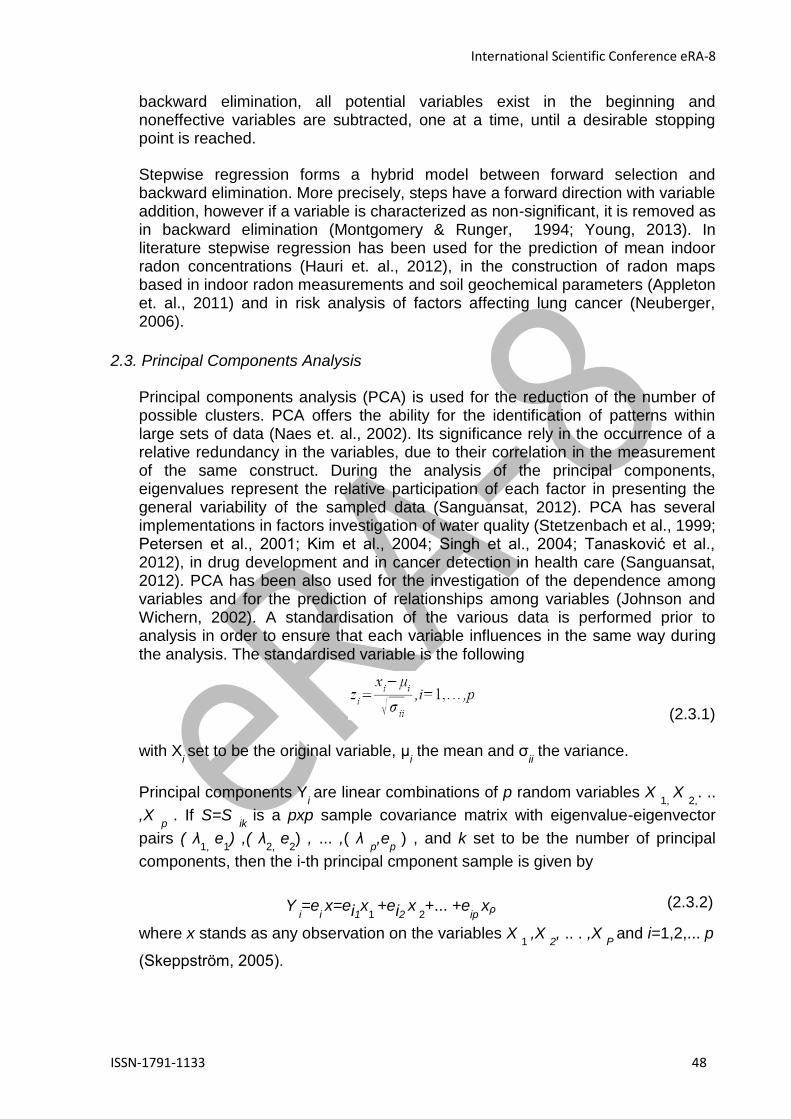
International Scientific Conference eRA-8
ISSN-1791-1133 48
backward elimination, all potential variables exist in the beginning and noneffective variables are subtracted, one at a time, until a desirable stopping point is reached.
Stepwise regression forms a hybrid model between forward selection and backward elimination. More precisely, steps have a forward direction with variable addition, however if a variable is characterized as non-significant, it is removed as in backward elimination (Montgomery & Runger, 1994; Young, 2013). In literature stepwise regression has been used for the prediction of mean indoor radon concentrations (Hauri et. al., 2012), in the construction of radon maps based in indoor radon measurements and soil geochemical parameters (Appleton et. al., 2011) and in risk analysis of factors affecting lung cancer (Neuberger, 2006).
2.3. Principal Components Analysis
Principal components analysis (PCA) is used for the reduction of the number of possible clusters. PCA offers the ability for the identification of patterns within large sets of data (Naes et. al., 2002). Its significance rely in the occurrence of a relative redundancy in the variables, due to their correlation in the measurement of the same construct. During the analysis of the principal components, eigenvalues represent the relative participation of each factor in presenting the general variability of the sampled data (Sanguansat, 2012). PCA has several implementations in factors investigation of water quality (Stetzenbach et al., 1999; Petersen et al., 2001; Kim et al., 2004; Singh et al., 2004; Tanasković et al., 2012), in drug development and in cancer detection in health care (Sanguansat, 2012). PCA has been also used for the investigation of the dependence among variables and for the prediction of relationships among variables (Johnson and Wichern, 2002). A standardisation of the various data is performed prior to analysis in order to ensure that each variable influences in the same way during the analysis. The standardised variable is the following
(2.3.1)
with Xi set to be the original variable, μ
i the mean and σ
ii the variance.
Principal components Yi are linear combinations of p random variables X
1, X
2,. ..
,X p
. If S=S ik
is a pxp sample covariance matrix with eigenvalue-eigenvector
pairs ( λ1,
e1) ,( λ
2, e
2) , ... ,( λ
p,e
p ) , and k set to be the number of principal
components, then the i-th principal cmponent sample is given by
Y i=e
i x=ei1x1
+ei2 x
2+... +e
ip xρ
(2.3.2)
where x stands as any observation on the variables X 1
,X 2, .. . ,X
P and i=1,2,... p
(Skeppström, 2005).

International Scientific Conference eRA-8
ISSN-1791-1133 49
2.4. One Way or multiway ANOVA
Analysis of variance (ANOVA) is considered as the generalization of a t-test to more than two statistical groups. ANOVA is divided in two categories: i) One way, where a single factor exists and ii) two way or multiway, where two or more factors exists. ANOVA is used for distributional assumptions about a set of effects in a model, with ability to extrapolate the inferences to a wider population, improve accounting for system uncertainty and the efficiency of estimation (Kéry, 2010). ANOVA has been implemented as the basic method for the statistical analysis of Radon concentrations in many studies (Manousakas et al., 2010; Papachristodoulou et al., 2010; Trevisi et al., 2012; Stojanovska et al., 2012; Cucoş et al., 2012; Ju et al., 2012). For the analysis of factors affecting indoor radon concentrations, initially each factor was analysed indepentedly. In such a way a first assumption for the weightiness of the effection of each factor is possible. In the next step, factors affection are no longer estimated independently; instead, factors influence each other and therefore are dependent. The aforementioned method, is called random-effects assumption of the analysis of variance (Kéry, 2010). ANOVA can be implemented only in sampling distributions similar to Gaussian ones, thus it was applied in the log distributions of radon measurements.
In order to construct the ANOVA table we measure how much the variability in Y variable is explained or not with the regression relationship of X variable. This table shows additionally the Mean Square Error (MSE). The overall variation in Y
is equal with the sum of regression variation and the error variation:
(2.4.1)
where ei=Y
i −Y
i ,i= 1,2 ,. .. ,n and Y
i=β
0+β
1 ⋅X
i+ε
ι,i= 1,.. . ,n
The ANOVA table involves the following elements:
i) The sum of squares for total ( SST ) n
SST=∑(Yi−Y)
2
(2.4.2)
i= 1
which is the sum of the squared deviations from the overall mean of Y . SST
is considered as a measure of the overall variation in the Y values.
ii) The sum of squared errors ( SSE ) which is the sum of squared
observed errors for the observed data and equals
n
SSE=∑(Yi−Y
i)2
(2.4.3)
i= 1
SSE is a measure of the variation in Y which is not explained by the
regression.

International Scientific Conference eRA-8
ISSN-1791-1133 50
iii) The sum of squares of the regression ( SSR ) defined as the difference
between SST and SSE
SSR=SST –SSE (2.4.4)
SSR is a measure of the total variation of Y that can be explained from the
regression with X variable.
iv) The mean of squares
(2.4.5)
called error mean square and the mean square of the regression ( MSR )
(2.4.6)
that equals with the SSR (Young, 2013).
The ANOVA table is defined as follows:
Source of
variation SS df MS F-value P(> F)
Regression
1
p-value
Error
n−2
Total
n−1
2.5. General MANOVA
Multivariate analysis of variance (MANOVA) is defined as a partition of the sum of
squares and the sum of the cross products (SSCP) matrix

International Scientific Conference eRA-8
ISSN-1791-1133 51
(2.5.1)
into independent Wishart matrices (Mathew, 1989). MANOVA is applied instead of a series of one-at-a-time ANOVAs. In several situations, the power of MANOVA is inferior to ANOVA of one variable at a time, however, MANOVA takes into account the intercorrelations among the dependent variables. Hence, MANOVA is considered more efficient over ANOVA for multivariate data (Stahle & Wold, 1990).
A MANOVA table includes the following elements:
i) The sum of squares and cross products for total ( SSCPTO ), which is the sum of squared deviations from the overall mean vector of the Y
i and equals to
(2.5.2)
SSCPTO is considered as a measure of the overall variation in the Y vectors.
ii) The sum of squares and cross-products of the errors ( SSCPE )
(2.5.3)
which is the sum of squared errors (residuals) for the data vectors. SSCPE is considered as a measure of the variation in Y that is not explained by the multivariate regression.
iii) The sum of squares and cross-products due to the regression (SSCPR) is defined as the difference between SSCPTO and SSCPE :
SSCPR=SSCPTO−SSCPE (2.5.4) SSCPR is a measure of the total variation in Y that can be explained by the regression with the predictors (Young, 2013).
The MANOVA table is defined as follows:

International Scientific Conference eRA-8
ISSN-1791-1133 52
3. RESULTS AND DISCUSSION
Fig. 1 presents characteristic residual plots calculated from the measured average concentrations of radon ( C ) and their logarithms ( log(C ) ). It is noted that the C values of Fig.1 correspond to time-integration over a year, constitute representative sample for Greece, were derived in accordance to international standards and delineate the radon profile of Greece (Nikolopoulos et al., 2002). In this consensus, Fig.1 is of significance since it may show actual tendencies regarding the randomness or predictability of the employed concentration sample. Indeed, completely randomised responses to normal-distribution either of C or log(C ) , would exhibit no deterministic normal-distribution's residuals and, hence, be completely described by stochastic processes. The normal probability plots of Figs 1a and 1b indicate, however, that the logarithms of the measured concentration followed normal distribution up to the 95% of log(C ) values, namely indicated that C values followed log-normal distribution. This is also evident from the shapes of the frequency distributions of the residuals. The frequency distribution of Fig.1a was clearly lognormal, while simultaneously that of Fig.1b, clearly normal. This is also of significance because all international large-scale radon surveys reported log-normal behaviour of indoor radon concentrations. The reason is rational thus why C values did not follow normal distribution as shown in the corresponding normal probability plot of Fig.1a. Under another view, the residual plots of log(C ) versus values fitted to normal-distribution, showed a random pattern for fitted residual values of log(C ) above 1.6. It is noted that a residual of 1.6 in log(C ) is consistent with uncertainty ζ
C
=39.8 Bq⋅m−3
in predicted C values. This, according to the recording capabilities of the employed dosimeters (Nikolopoulos et al., 1998), accompanies high C
values, namely C values above the EU action limit of 200 Bq⋅m−3
. Moreover, the majority of predicted residuals were below 1.2. This is very significant because this residual range is consistent with concentrations usually addressed, namely
between 10-120 Bq⋅m−3
. Other factors may affect concentrations in this range and surely the potential factors could not be continuous under the normal distribution. Indeed, the Versus Fits diagram of Fig1.a shows characteristic predictability different from the normal distribution for the residual C range below
75 Bq⋅m−3
. On the other hand, the residual versus observation order did not
showed tendencies for concentrations up 160 Bq⋅m−3
either in the concentration order (Fig1a) or the order of concentration's logarithm.

International Scientific Conference eRA-8
ISSN-1791-1133 53
Fig.1 Residual plots of (a) radon concentration and (b) logarithm of radon concentration.
All measurements are shown. Each plot contains (I) percentage of residuals versus
residual, (II) frequency distribution of the residuals, (III) residual versus fitted values
according to C for a and log(C ) for b and (IV) residual versus observation order.
Table 1 presents the analysed factors, factor levels and level values with their corresponding description. Data of Table 1 were formulated in accordance to the contents of the 963 questionnaires which were filled during the radon survey of

International Scientific Conference eRA-8
ISSN-1791-1133 54
Greece. It is noted that these questionnaires were developed in agreement to other national surveys. The majority of factors exhibited 3-4 levels. This is noteworthy in any related analysis, since a multi-level collection of factors can distract results especially for limited number of measurements. Factor (L) was 5-level marking the usual situation of apartment dwellings in big cities of Greece. Nevertheless, this 5-level factor is easily convertible to a lower-level one. Factor (F) was free to fill, so a 6 level collection was finally achieved.
Table 1. Descriptions of used factors (qualitative)
It is well identified that Gauss distribution offers a rigid and justified pathway for statistical analysis Since concentrations' logarithms followed the distribution of Gauss, log(C ) was considered favourable. Hereafter any analysis was conducted only on log(C ) . Table 2 presents the unusual observations in log(C ) values accounting that these followed normal distribution, viz. were treated according to the distribution of Gauss. Leverage points were considered to be those observations corresponding to extreme or outlying values of log(C ) in a manner that any lack of neighbouring observations implied that the fitted Gaussian regression model passed close to the particular observation. In specific, leverage points were calculated by moving all points one-by-one up or down and calculating the proportionally constant (leverage) of the change of the corresponding Gaussian fitted value. Outliers were calculated as the observations that presented residuals above 1.5 times the interquartile range. According to Table 2, eight outlier and two leverage residual points were identified. In any case, unusual log(C ) values were approximately 0.1% of the total concentration sample size. Therefore, they constituted a negligible part of measurements. Importantly, however, the latter finding indicates that only a small portion (<0.1%)

International Scientific Conference eRA-8
ISSN-1791-1133 55
of Greek dwellings presented unusual concentrations. Considering that high unusual concentration extremes may associate with high human radiation burden, this fact implies that indoor radon in Greece may not lie in the international extremes. Emphasis should be stressed also on the fact that outlier data affect any type of fit and should be removed prior to regression analysis, whereas, leverage point may or may not affect. For this reason, all outlier and leverage points were finally removed from the dataset.
Table 2. Unusual Observations for log(C ) . R denotes observations with large standardized
residual. X denotes observations that gave large leverage. O denotes the number of
observation, SE-F the standard error of the fit and SR the standardised residual.
Table 3 presents the combinations to define the best subsets from the nine factors of Table 1 for the regression of log(C ) . As in Table 2, regression was linear to the factors employed in each entry of Table 1.. Mallow's C
p was
calculated for any subset of k ,k ≤ p of explanatory variables, as
where SSE p
was the residual sum of squares for the subset
model containing p explanatory variables counting the intercept (i.e., the number of parameters in the subset model) and n is the sample size. It should be emphasised that, acceptable models in the sense of minimizing the total bias of predicted values are those models for which C
p approaches the value p , i.e.,
those subset models that fall near the line Cp
= p in a plot of Cp
against p for the
collection of all subset models under consideration. Under this view, only the combination of all factors except factor G (Ground Type, Table 1) constitute an explanatory subset for minimising total bias.

International Scientific Conference eRA-8
ISSN-1791-1133 56
Table 3. Best subsets regression: log(C ) versus all factors. R2
, adjusted Radj2, Mallow's Cp (MCP)
and standard error (SE) in each subset is presented. V denotes the number of factors included within each model.
Table 4 presents the results of stepwise regression of log(C ) versus all factors. Through stepwise regression, a linear model was sought containing only those variables which were significant in modelling log(C ) . The qualitative factor levels of Table 1 were employed in their original values so as to be transformed to quantitative variables. It should be stressed, that stepwise regression is particularly useful when there are many possible explanatory (independent) variables. Some of these variables may be highly correlated with each other and therefore may explain the same variation in the response and not be independently predictive. Some may also not influence the response in any meaningful way. For this reason, employing high alpha values for the error probability in Table 4, only three factors were finally selected, and these after the third step. It is noted that probability values, p , and alpha values, a , are related as p=1−a and thus the results of Table 4 correspond to the 50% significance level either for accepting entering of a certain factor or its removal. According to Table 4 the main factors found to influence indoor radon concentrations were wall, level and contact. In specific, factor contact exhibited p -value of 0,162, factor level, 0,131 and factor wall 0,276 (error probability 50%). This implies that at a significance level <17% level and contact affect indoor radon concentration, while

International Scientific Conference eRA-8
ISSN-1791-1133 57
at the 30% significance level, all three factors affect. These results, however, provide vague evidence on the null hypothesis, namely that the above factors actually affect. This is also indicated by the small value of MCP in reference to an
accepted well value of 3 for two factors and 4 for 3 factors. Moreover, since R2
exhibited maximum value of 2.92, only a small percent of the total variance (<3%) can be described by a linear model of the three factors of Table 4.
Table 4. Stepwise Regression: log(C ) versus all factors. Value of Alpha-to-Enter was 0,5 and of
Alpha-to-Remove 0,5. P-values represent calculated error probabilities and T-values, the
corresponding values of t-student's test for the comparison of a P-value with a . The constants of
the linear fit at each step are shown in first row. Bold values represent the corresponding slopes
of each factor at each step. MCP is the Mallow's C p .
According to data presented so-far, no single factor or linear subset of factors, could describe sufficiently the variance of the analysed radon concentration data. This implies that a multivariate set of factors could be probably more adequate. Table 5 presents the unrotated factor loadings together with the corresponding communalities according to principal component analysis, applied however to radon concentrations. It is very interesting that, although factor 1 is loaded to five factors, the remaining three are only loaded to one single factor each. More

International Scientific Conference eRA-8
ISSN-1791-1133 58
specifically, 16,2% of the total variance may be described by factor 2 loaded only to the construction year. 12,3% of the total variance could be attributable to factor 3 loaded mainly to the existence of basement and 10.8% to the existence of contact. A very important finding of Table 5, however is that since the loadings of factor 1 to level, building type and construction year are negative in respect to the one of C , it is rational to accept that concentrations would increase as level, building type and construction year are decreased. According to Table 1, this implies that ground floor dwellings tend to present higher radon concentrations. This is rational since the lower the floor, the higher is the contribution of soil's exhalation in indoor radon. Similar are the results for normal or sloppy dwellings (especially when ground floored). Also detached houses tend to present higher concentrations, since other types offer pathways for radon's interchange between dwellings in contact. Significant is also that aged dwellings, especially those of the previous century, presented higher radon concentrations. The latter finding is also reinforced by the positive loading the building material of the wall, especially due to its rather high loading. Since higher wall values correspond to rock materials, it can be supported that higher concentrations are addressed in dwellings of the beginning of the twentieth century made of rocks. To some degree the results were supported by Table 4, since the dwelling's level and building material were considered to be more significant compared to the other factors.
Table 5. Unrotated factor loadings and communalities for 4 principal factors. The factor
correlations exceeding the cut-off limit of 0.5 are marked in bold.

International Scientific Conference eRA-8
ISSN-1791-1133 59
Additionally to the analysis presented so-far, one-way ANOVA was applied to single-factor data from the whole data set. Analysing factor L in its full depth, an F value of 2,551 was calculated whereas the critical F value at the 95% confidence interval -CI is 2,03. These values imply that with p =0.014 results from the various different levels collected did not differ significantly. However when the full dwelling-level data were reorganised in 3-levels (ground floor, first floor and upper floors) F was found equal to 7,156 while the corresponding critical value at the 95% CI is 3..01 with corresponding value p =0.000877. This finding is significant since it implies that with p <0.001 lower level dwellings present higher indoor radon concentrations. This finding reinforces the findings of Table 5. Further evidence were provided by reorganising dwelling-level data in 2 levels, namely ground floor and higher floor dwellings. Applying t-test to the average concentrations it was calculated that at p <0.001 ground floor dwellings presented higher radon concentrations. Analysing factor C with one-way ANOVA, an F value of 0,893 was calculated whereas the critical F value at the 95% CI is 2,624. Namely, at p <0.001 different C-factor level dwellings did not present differences. Similar was the outcomes of the one-way ANOVA for factor F. Non significant variations were addressed, since calculated F value was 1,298 and the critical value at 95% CI, 2,119. On the contrary, the one-way analysis of factor W, provided and F value of 4,314 with a critical value at 95% CI of 2,624 and an associated p value of 0.0051. The latter finding was associated with a tendency of higher concentrations of rock dwelling.
Table 6 presents the results of the general MANOVA method. More significant factros were those given in Table 6. These results support further the findings of the one-way ANOVA and the results of the stepwise regression analysis. Non-significant statistical interactions between any combinations of factors were detected by General MANOVA

International Scientific Conference eRA-8
ISSN-1791-1133 60
Table 6. General MANOVA for log(C). Cut-off Limit for significance level < 30%
4. CONCLUSION
Statistical analysis of the data revealed that approximately 0.1% of the dwellings exhibited outlier radon concentrations. Noteworthy statistical correlations were detected between indoor radon concentration and the factors: "height from ground" and "building material". Results of current work strengthened the considerations and provided weak evidence for the correlation of factors like "floor type" and "construction year" with radon concentrations. Minor association was detected with the factor "building contact". Significant differences were detected in results produced by some of the applied multivariate methods.
ACKNOWLEDGEMENT
This work was co-financed by Greece and the European Union under the European Social Fund NSRF 2007-2013 (Thales). Managing Authority: Greek Ministry Of Education & Religious Affairs, Culture & Sports.
Bibliography
UNSCEAR (United Nations Scientific Committee on the Effects of Atomic Radiation), 2000.
Sources and Effects of Ionizing Radiation. Report Vol.I, AnnexB: Exposures from Natural Radiation Sources. UNSCEAR, New York.
A STUDY OF ENVIRONMENTAL RADIOACTIVITY MEASUREMENTS IN THE SAMSUN PROVINCE, TURKEY, B. Kucukomeroglu1, F. Maksutoglu1, N. Damla2,*, U. Cevik1 and N. Celebi3, Radiation Protection Dosimetry (2012), Vol. 152, No. 4, pp. 369– 375
IARC (International Agency for Research on Cancer). Monographs on the evaluation of carcinogenic risks to humans. Man-made mineral fibres and radon, 43; 1988. Lyon.
ICRP 65 (International Commission on Radiological Protection). Protection against radon222 at home and at work. Oxford: Pergamon Press; 1994.
UNSCEAR (United Nations Scientific Committee on the Effects of Atomic Radiation). Annex E: sources-to-effects assessment for radon in homes and workplaces. New York: United Nations; 2006.
Correction factors for determination of annual average radon concentration in dwellings of Poland resulting from seasonal variability of indoor radon , K. Kozak a,n, J.Mazur a, B.Koz"owska b,

International Scientific Conference eRA-8
ISSN-1791-1133 61
M.Karpin´ ska c, T.A.Przylibski d, K.Mamont-Cies´la e, D. Grza˛dziel a, O.Stawarz e, M.Wysocka f, J.Dorda b, A.Z˙ebrowski d, J.Olszewski g, H.Hovhannisyan a,
M. Dohojda h, J.Kapa"a c, I.Chmielewska f, B.K"os b, J.Jankowski g, S.Mnich c,
R.Ko"odziej f , Applied Radiation and Isotopes 69 (2011) 1459–1465, Indoor radon
measurements in the city of Valencia , F. Tondeur a,n, J.Ro´ denas b, A.Querol b, J.Ortiz b,
B.Juste b , Applied Radiation and Isotopes 69 (2011) 1131–1133 Radon level and indoor gamma doses in dwellings of Trabzon, Turkey A. Kurnaz a, B.K¨ uc-
¨uk¨omero˘glu a, U.C-evik a,n, N.C-elebi b , Applied Radiation and Isotopes 69 (2011) 1554–1559
Assessment of Seasonal Variation of Indoor Radon Level in Dwellings of Some Districts of Azad Kashmir, Pakistan, Muhammad Rafiquea S.U. Rahmanb Tahir Mahmooda Said Rahmanc Matiullahd, Indoor Built Environ 2011;20;3:354–361
NATIONAL RADON SURVEY IN KOREA Yongjae Kim1,*, Byung-Uck Chang1, Hong-Mo Park1, Chang-Kyu Kim1,2 and Shinji Tokonami3, Radiation Protection Dosimetry (2011), Vol. 146, No. 1–3, pp. 6–10
SURVEY OF RADON AND THORON IN HOMES OF INDIAN HIMALAYA, Rakesh Chand Ramola, Radiation Protection Dosimetry (2011), Vol. 146, No. 1–3, pp. 11–13
Assessment of seasonal indoor radon concentration in dwellings of Western Haryana, Rohit Mehra a,*, Komal Badhan a, Sandeep Kansal b, R.G. Sonkawade, Radiation Measurements 46 (2011) 1803e1806
Seasonal indoor radon concentration in FYR of Macedonia Zdenka Stojanovska a,*, Jovan Januseski a, Peter Bossewb, Zora S. Zunic c, Tore Tollefsen d, Mimoza Ristova, Radiation Measurements 46 (2011) 602e610
Seasonal variation of radon concentrations in UK homes, J C H Miles, C B Howarth and N
Hunter, J. Radiol. Prot. 32 (2012) 275–287 PRELIMINARY RESULTS FROM AN INDOOR
RADON THORON SURVEY IN HUNGARY G. Szeiler1, J. Somlai1, T. Ishikawa2, Y. Omori2,
R. Mishra3, B. K. Sapra3, Y. S. Mayya3, S. Tokonami4, A. Csorda´s5 and T. Kova´cs1,
Radiation Protection Dosimetry (2012), Vol. 152, No. 1–3, pp. 243–246 RADON IN FINNISH
APARTMENT BUILDINGS T. Valmari*, H. Arvela and H. Reisbacka, Radiation Protection
Dosimetry (2012), Vol. 152, No. 1–3, pp. 146–149 Thorough investigations on indoor radon in
Băiţa radon-prone area (Romania) Alexandra Cucoş (Dinu) a, Constantin Cosma a, Tiberius
Dicu a,⁎, Robert Begy a, Mircea Moldovan a, Botond Papp a, Dan Niţă a, Bety Burghele a,
Carlos Sainz, Science of the Total Environment 431 (2012) 78–83
Indoor radon levels in Greek schools, A. Clouvas*, S. Xanthos, G. Takoudis, Journal of
Environmental Radioactivity 102 (2011) 881e885
Proukakis, C., Molfetas, M., Ntalles, K., Georgiou, E., Serefoglou, A., 1988. Indoor radon measurements in Athens, Greece. In: British Nuclear Energy Society Conference on health effects of low dose ionizing radiation-recent advances and their implications. BNSE, London, 177–178.
Georgiou, E., Ntalles, K., Molfetas, A., Athanassiadis, A., & Proukakis, C., 1988a. Radon measurements in Greece. In Radiation Protection Practice. New York, Pergamon Press, IRPA 7, Volume I, 125–126.
Papastefanou, C., Stoulos, S., Manolopoulou, M., Ioannidou, A., Charalambous, S., 1994. Indoor radon concentrations in Greek apartment dwellings. Health Physics 66 (3), 270–273.
Ioannides, K.G., Stamoulis, K.C., Papachristodoulou, C.A., 2000. A survey of 222Rn concentrations in dwellings of the town of Metsovo in North-Western Greece. Health Physics 79 (6), 697–702.
Clouvas, A., Xanthos, S., Antonopoulos-Domis, M., 2007. Pilot study of indoor radon in Greek

International Scientific Conference eRA-8
ISSN-1791-1133 62
workplaces. Radiat. Prot. Dosim. 124, 68e74.
Indoor radon levels in Greek schools A. Clouvas*, S. Xanthos, G. Takoudis , Journal of Environmental Radioactivity 102 (2011) 881e885
Nikolopoulos, D., Louizi, A., Koukouliou, V., Serefoglou, A., Georgiou, E., Ntalles, K., Proukakis, Ch, 2002. Radon survey in Greece-risk assesment. J. Environ. Radioact. 63, 173e186.
Baixeras, C., Font, L., Robles, B. and Gutie´rrez, J. Indoor radon survey in the most populated areas in Spain. Environ. Int. 22, S671–S676 (1996)
Gallelli, G., Panatto, D., Lai, P., Orlando, P. And Risso, D. Relevance of main factors affecting radon concentration in multi-storey buildings in Liguria (Northern Italy). J. Environ. Radioact. 39, 117–128 (1998).
Bochicchio, F. et al. Annual average and seasonal variations of residential radon concentration for all the Italian Regions. Radiat. Meas. 40, 686–694 (2005).
Bossew, P. and Lettner, H. Investigations on indoor radon in Austria, Part 1: Seasonality of indoor radon concentration. J. Environ. Radioact. 98, 329–345 (2007).
Denman, A.R., Groves-Kirkby, N.P., Groves-Kirkby, C.J., Crockett, R.G.M., Phillips, P.S., Woolridge, A.C., 2007. Health implications of radon distribution in living rooms and bedrooms in U.K. dwellings e a case study in Northamptonshire. Environment International 33 (8), 999e1011
Soil and building material as main sources of indoor radon in Bait¸ a-S¸ tei radon prone area (Romania) Constantin Cosma a, Alexandra Cucos¸ -Dinu a, Botond Papp a,*, Robert Begy a, Carlos Sainz, Journal of Environmental Radioactivity 116 (2013) 174e179
Radon exhalation rate and natural radionuclide content in building materials of high background areas of Ramsar, Iran E. Bavarnegin a, N. Fathabadi b,*, M. Vahabi Moghaddam a, M. Vasheghani Farahani b, M. Moradi b, A. Babakhni b, Journal of Environmental Radioactivity 117 (2013) 36e40
Introduction to WinBUGS for Ecologists, Marc Kéry 2010, Pages 115-127, Chapter 9
Indoor radon levels in schools of South-East Italy, Rosabianca Trevisi, Federica Leonardi*, Carla Simeoni, Sabrina Tonnarini, Miriam Veschetti, Journal of Environmental Radioactivity 112 (2012) 160e164
Indoor radon measurements in a Greek city located in the vicinity of lignite-fired power plants, M. Manousakas, A. Fouskas, H. Papaefthymiou, V. Koukouliou, G. Siavalas, P.
Kritidis, Radiation Measurements 45 (2010) 1060e1067 Exposure to indoor radon and natural gamma radiation in public workplaces in northwestern
Greece, C.A. Papachristodoulou, D.L. Patiris, K.G. Ioannides, Radiation Measurements 45 (2010) 865e871
Study on measurement and quantitative analysis of Radon-222 emitted from construction materials, Yong-Jin Ju, Young-Hwan Ryu, Kyung-Rae Dong, Jae-Hwan Cho, Hae-Kag Lee, Woon-Kwan Chung, Annals of Nuclear Energy 49 (2012) 88–95
Principal Component Analysis – Multidisciplinary Applications, Parinya Sanguansat, February 2012 , Rijeka, Croatia, InTech, ISBN 978-953-51-0129-1
Multivariate statistical analysis of hydrochemical and radiological data of Serbian spa waters, Irena Tanasković, Dusan Golobocanin, Nada Miljević, Journal of Geochemical Exploration 112 (2012) 226–234
T. Naes, T. Isaksson, T. Fearn and T. Davies, A User-Friendly Guide to Multivariate Calibration and Classification. NIR Publications, Chichester (2002)

International Scientific Conference eRA-8
ISSN-1791-1133 63
Johnson, R. and Wichern, D. 2002. Applied Multivariate Statistical Analysis. Prentice Hall, New Jersey, 426-476 pp
RADON IN GROUNDWATER-INFLUENCING FACTORS AND PREDICTION METHODOLOGY FOR A SWEDISH ENVIRONMENT, Kirlna Skeppström, November 2005, ISBN 91-7178-208-7, KTH Land and Water Resources Engineering
Regression Methods, Derek Young, STAT 501, Pennsylvania State University, 2013
A prediction model for assessing residential radon concentration in Switzerland, Dimitri D. Hauri, Anke Huss, Frank Zimmermann, Claudia E. Kuehni, Martin Röösli, Journal of Environmental Radioactivity 112 (2012) 83e89
Comparison of Northern Ireland radon maps based on indoor radon measurements and geology with maps derived by predictive modelling of airborne radiometric and ground permeability data, J.D. Appleton, J.C.H. Miles, M. Young, Science of the Total Environment 409 (2011) 1572–1583
D. Montgomery, G. Runger, Applied Statistics and Probability for Engineers, Wiley, 1994
Risk factors for lung cancer in Iowa women: Implications for prevention, John S. Neuberger , Jonathan D. Mahnken, Matthew S. Mayo, R. William Field, Cancer Detection and Prevention 30 (2006) 158–167
MANOVA in the Multivariate Componets of Variance Model, T. Mathew, JOURNAL OF MULTIVARIATE ANALYSIS 29, 30-38 (1989)
Multivariate Analysis of Variance (MANOVA), L.STAHLE, S. WOLD, Chemometrics and Intelligent Laboratory Systems, 9 (1990) 127-141
Kenney, J. F. and Keeping, E. S. (1962) "Linear Regression and Correlation." Ch. 15 in Mathematics of Statistics, Pt. 1, 3rd ed. Princeton, NJ: Van Nostrand, pp. 252-285

International Scientific Conference eRA-8
ISSN-1791-1133 64
Preliminary study of distribution of background EMR in Greek apartment
dwellings
D. Nikolopoulos1
, P. Yannakopoulos1
, E. Petraki1,2
, S. Kottou3
, Α.Louizi3
, N.
Gorgolis1
, X. Argyriou1
, S. Potozi4
, T. Sevvos1
, D. Koulougliotis4
, E. Vogiannis5
, I.
Zisos6
, G. Kefalas4
, R. S. Lorilla4
, A. Zisos6
1
Department of Computer Electronic Engineering, TEI of Piraeus, Greece, Petrou Ralli & Thivon 250, 12244,Aigaleo,Athens, Greece
2
Department of Engineering and Design, Brunel University, Kingston Lane, Uxbridge, Middlesex UB8 3PH,London, UK.
3
Medical Physics Department, Medical School, University of Athes, Mikras Asias 75, 11527, Goudi,, Athens,Greece.
4
Department of Environmental Technology and Ecology, Technological Educational Institute (TEI) of Ionianslands, Neo Ktirio Panagoula, 29100, Zakynthos, Greece.
5
Model School of Smyrna, Lesvou 4, 17123, Nea Smirni, Athens, Greece. 6
TEI of Piraeus, Greece, Petrou Ralli & Thivon 250, 122 44,Aigaleo,Athens, Greece
*
e-mail: [email protected], web page: http://env-hum-comp-res.teipir.gr/
ABSTRACT:
The main purpose of this study was to investigate different electromagnetic sources and characterize different environmental categories, namely urban, suburban, rural areas offices and workplaces. Based on the suggestions of WHO International EMF Project‘s RF Research Agenda and ICNIRP, measurement surveys are conducted to characterize population exposures from all radio frequency (RF) sources. Emphasis is placed on new wireless technologies, mobile telecommunications and DECT telephony. Up-to-date 70 indoor locations were accessed. Additionally, focused research has been carried out to identify places of interest further and to standardize the protocol of measurements. Maximal total electric field values were below 5 V/m in most case, however increased values of up to 3 kV/m were addressed near high-power voltage lines. Wi-Fi frequencies were identified as the main electromagnetic source indoors. Rural areas presented significantly lower electric field values; approximately 3-5 times lower than those of urban areas. Magnetic field values were in most cases below 0.1 mG. Increased values of up to 60 mG were observed near high voltage power lines.
1. INTRODUCTION
Daily, we are exposed, to electromagnetic radiation, coming from the environment as from the sun, the outer space, even from the earth itself. Since

International Scientific Conference eRA-8
ISSN-1791-1133 65
the begging of the 20th
century, however, there has been an increased exposure of the population to non-ionizing radiation, especially in the LF-EMR due to the increased use of radios, radars, televisions, PCs, mobile phones, Wi-Fi, DECT bases and so on. All these technological achievements have raised concerns about the health problems that may occur and are associated to the increased use of these devices, involving an increased exposure to EMR. (NRPB 2003; HPA 2004a, 2004b; Valberg et al 2007; Ahlbom et al 2008; SCENIHR 2007, 2009).
Apart from LF-EMR we are also exposed, more and more, to radio frequencies (RF). In every case, the exposure to EMR sources is measured in the surrounding space of the object and the distance from the device and in the case of directional antennas from the proximity to the main beam. The field intensity decreases, often rapidly, with distance (IEEE 2004, 2005a, 2005b; IEC 2005; WHO 2002, 2006a, 2006b, 2011).
1.1.RF
Since the early 90s, there is an increased exposure to RF radiation due to the presence of mobile phones in the market which resulted in steady and rapid growth of DECT base stations. More than 2 billion people worldwide are now using mobile phones. In Europe, the percentage of users reaches up to 80%. (Scenihr 2007). Despite the increasing development of new technologies that use RF, the knowledge we have about the effect on human exposure, is minimum.
In a typical home, the RF exposure may be caused by outdoor factors such as the radio, the television, and the mobile phone antennas, but also indoor factors such as the operation and the use of mobile phones, DECT base stations, WLAN, or even from a microwave oven. The transmitters of the radio and television have a large coverage area and therefore operate at relatively high power levels up to 1 MW (Dahme 1999). However, the high levels of operation do not cause major exhibition of the population because they are in sparsely populated areas. Power levels inside a building can be from 1 to 100 times lower than those outside the building (Schüz and Mann 2000) and even inside the building the exposure may vary from floor to floor. For example, the exposure on the higher floors was double (and more variable) compared to the lower floors of a building. (Anglesio et al. 2001).
1.2.Mobile phones
Most mobile phones in Europe use GSM900, GSM1800 (Global System for Mobile Communications) or UMTS (Universal Mobile Telecommunications System) which are the latest technology and operate in 1900-2200MHz. The radiation we receive from a mobile phone depends on various factors such as the

International Scientific Conference eRA-8
ISSN-1791-1133 66
characteristics of the device, particularly the type and the location of the antenna, the distance and the way we keep the mobile, the distance that the antenna of each company is situated, on whether the user is in motion (for example, inside a car) and most importantly, the adaptive power control, which may reduce the emitted power by orders of magnitude (up to a factor of 1,000). In areas where are many phone-users, the mobile phones can work at maximum power for quite long time. Inside the buildings, the power levels of mobile phones are on average higher than outdoor ratios, because of the shielding materials. (Scenihr 2007; Ahlbom 2004)
1.3.DECT
Wireless phones and their base stations (DECT), like all wireless devices, generate radio waves but the exposure to these sources is usually lower than to mobile phones. A typical cordless phone, found in a house, produces about 10 mW of power, considerably less than a mobile phone and this is because the signals have to travel only a few meters compared to the signal of a mobile phone that can even travel for kilometers. What we need to examine is the field strength of its base station. The maximum time-averaged power level for a DECT base station is the same while for a mobile phone handset is 250 mW. However, the exposure is less because the cordless phone base station is not held to the head, and the field strength falls rapidly with distance (Scenihr 2007).
1.4.WLAN
A terminal WLAN, for domestic use, has a maximum power of 200 mW but the average power is much less, because it depends on the traffic. Typically, the field
intensity is below 0,5 mW / m2
, so the exposure to them is lower than that in the mobile phones. In some cases, however, the exposure to RF fields from WLAN and DECT base stations can overcome GSM and UMTS (Scenihr 2007).
2.MATERIALS AND METHODS
2.1.Measurement locations
The measurements of this research were made in houses in different regions of Attica and in several areas of the Greek province. By now they have been performed 70 measurements indoors. The aim of this research is to identify the areas of interest and to determine the protocol for the future measurements.
2.2.Measurement procedure
The measurements were performed using Aaronia spectrum analyzer (HF & NF) machines which show the exact frequency and the signal strength of the sources including RF and EMF. These devices are widely and successfully used in industry, research, schools and workshops RF, mobile phones, transmission towers, WLAN, DECT, Wi-Fi, Bluetooth, monitors, televisions, power lines and so

International Scientific Conference eRA-8
ISSN-1791-1133 67
on, as with the EME spy Information (ANTENNESSA).The highest threshold of 5.02 V/m of the equipment used, limited several measurements which led us to the possible use of any other device with no highest limit, in order to measure the exact value in V/m existing in the area. All measurements given by the diagrams of this presentation are mean values. The frequencies of EME for the measured regions are defined in Table 1.
Table1. Frequency range
3.METHODS
The procedure followed was in accordance with the agreed protocol. All the measurements which were conducted with ANTENNESSA where done from the middle of each room and those that were conducted with the machineries of Aaronia spectrum analyzer (HF and NF) where done in various parts of the residencies, at distances of 0m, 1m, 2m from the devices (televisions, Wi-Fi, mobile phones). In some of the areas of interest, we decided to make targeted sequential measurements by enabling and disabling some devices, such as the microwave oven (MWO), the Wi-Fi and the mobile phones, by making calls to other mobile phones during the measurement. The time of measurements was set at 10 to 15 minutes. The above criteria were considered as standardization compromise during real measurement practice. In addition, all remaining factors were recorded.
4.RESULTS
I.TARGETED EXPERIMENTS I.4.1.Agricultural areas
The following series of measurements were carried out in a rural area in Evia, Almyropotamos, 160 Km from Athens. Totally ten measurements with various

International Scientific Conference eRA-8
ISSN-1791-1133 68
conditions were taken. Existence of a microwave oven and a DECT phone was detected. The microwave oven was not switched on, so its existence is neglected. A PC used for the measurements was equipped with a USB Internet connection (provided by WIND, with emitting frequency in the range of 900 MHZ). No visible antenna of mobile telephony and no high voltage carrier lines were in the region. Also no Wi-Fi device was in the building block. The measurements were performed with EME spy Information (ANTENNESSA). According to the agreed protocol all measurements were carried out in the middle of the room. 120 samples were taken (8 min) (Fig 1) with the only possible emitting device plugged in, but not in use!.
Fig.1 Measurements with the DECT device plugged in
From the previous diagram we decided to unplug the DECT phone and measure the EMF. So 144 samples were taken (12 min) (Fig 2) showing a difference in the DCT region. (It is possible that the other two co-existing households of the building block have a DECT phone plugged-in, but not in operation. After questing the neighbors NONE in the building had a Portable device BUT the neighboring buildings, being apart at least 20-50 meters YES in both directions).
Fig.2 Measurements with no device on (Portable phone unplugged)

International Scientific Conference eRA-8
ISSN-1791-1133 69
Fig.3 Measurements in the balcony (outside the building block)
The next step was to measure the outdoor EMF to compare it with the previous indoor one. 144 samples were taken (12 min) (Fig 3). A possible DECT communication or call ring appears in the waveform from a neighbors‘ device.
In order to examine the contribution of the building‘s EMF we measured in a nearby old house made from stone the existing field for the same duration (12 min) (Fig.4) We can see a decrease in the signal of the DECT phones as they are away approximately 60 meters.
Fig.4 Measurements in a stone made house near a Wi-Fi emitting base (Internet)

International Scientific Conference eRA-8
ISSN-1791-1133 70
Fig.5 Measurements in a Taverna (Public Area)
Similar behaviour appears in Fig.5 Slight increase of the Wi-Fi signal is due to the existence of a Wi-Fi emitter in a public place 40 meters away. The three picks appearing in Fig. 6 are due to a call to a mobile phone. (three ringing call in the 1710-1785 MHz range appears in the range of DTX. (Fig.6))
Fig.6 Analytical measurements of Fig.5
The measurements were taken away from the computer device in the middle of the room and away from the Computer.

International Scientific Conference eRA-8
ISSN-1791-1133 71
Fig. 7 Measurements with a WIND 3G USB device plugged in (5 min)
Fig. 8 Analytical measurements with a WIND 3G device plugged in (5 min)
The UTX component (1920-1980 MHz) shows significant variation. The next step was to examine the case where a mobile device was in use simultaneously with a portable one. Figs. 7and 8 show this behaviour during the call.

International Scientific Conference eRA-8
ISSN-1791-1133 72
Fig. 9 Forced call from the DECT to a mobile mean values
Fig. 10 Forced call from the DECT to a mobile
It was clear that we should examine closer the influence of any mobile device to the signal. We studied initially the contribution of the 3G-USB connected to the PC. Three measurements depending on the distance from the receiving point were carried out.

International Scientific Conference eRA-8
ISSN-1791-1133 73
Fig. 11 Measurements with a USB- 3G WIND 25 cm away (12 min)
Fig. 12 Measurements with a WIND 3G 25 cm (12 min)
Notice the upper threshold existing!!!! In 5.02 V/m. The total duration of the measurements was 12 min.

International Scientific Conference eRA-8
ISSN-1791-1133 74
Fig. 13 Measurements with a WIND 5 cm (12 min)
Fig. 14 Measurements with a WIND 3G 5 cm (12 min) NOTICE the upper threshold

International Scientific Conference eRA-8
ISSN-1791-1133 75
Fig. 15 Measurements with WIND 3G on PC ON at a distance of 0 cm
Fig. 16 Measurements with a WIND 3G PC ON at a distance of 0 cm
I.4.2.Athens area
The next measurements were carried out in locations around Athens. At Faliron, Niriidon Street, in Rafina and In Technological Educational Institute (TEI) of Piraeus, Petrou Ralli and Thivon Avenue under different conditions in the New Auditorium, at the secretary office and Electronics Lab of Building E.
At the Faliro location there‘s no DECT in the house but two existing ones on floor 1 and floor3 above the basis of the Wi-Fi

International Scientific Conference eRA-8
ISSN-1791-1133 76
Fig.17 Faliro Salon (no device in the room)
Fig.18 Faliro kitchen (equipped with a MWO not in Use
Higher lower value for Wi-Fi (90-103) (88-103)
From the Figures 17 and 18 we observe that, although, the Wi-Fi was disabled and we were in another room, the values were almost the same (0, 94 V/m and 0, 96 V/m respectively). We also had a small sign at the DECT region, of 0, 08 V/m, which was apparently due to DECT on other floors and another sign in UMTS region, of 0, 23 V/m.
The next three measurements (Figures 19a, b, c) were done in the children's room of the house, in three different days, to see if the EMR possibly present inside it is stable.

International Scientific Conference eRA-8
ISSN-1791-1133 77
Fig.19a Faliro Child’s room (room3) 31/5/2013 Wi-Fi (96-111)
Fig.19b Faliro Child’s room (room3) 11/5/2013 Wi-Fi (88-101)
Fig.19c Faliro Child’s room (room3) 12/5/2013 Wi-Fi (89-136)
As we can see, in all three measurements, the EMR was stable, with the Wi-Fi and UMTS rx to prevail. Also in this case, the Wi-Fi was disabled and in an

International Scientific Conference eRA-8
ISSN-1791-1133 78
adjoining room.
Fig.20a Faliro Child’s room with an Apple mobile connected to Facebook.
Fig.20b Detailed Faliro Child’s room with an Apple mobile connected to Facebook
In the above measurement (Figures 20a, b), we were connected to the internet using a mobile phone of the latest technology and we see that nothing has changed in our values.

International Scientific Conference eRA-8
ISSN-1791-1133 79
Fig.21a Faliro Wi-Fi ON measured 50 cm away
Fig.21b Detailed Faliro Wi-Fi ON measured 50 cm away
In this case (Figures 21a, 21b), we enabled the Wi-Fi and we measured within 50 cm from the device. We observe that the values of the Wi-Fi were almost double while all the others remain, approximately, the same.

International Scientific Conference eRA-8
ISSN-1791-1133 80
Fig.22a Faliro Wi-Fi OFF measured 50 cm away
Fig.22b Detailed Faliro Wi-Fi OFF measured 50 cm away
When we disabled the Wi-Fi, its prices were reduced again, at the same levels as
before.
In Rafina there was a Wi-Fi and a MWO in the hall and NO DECT in the house but the neighbours do have a DECT phone (beneath and aside)
The following two measurements (Figures 23a, 23b) we decided to make them, one with disabled Wi-Fi and the other one with enabled.

International Scientific Conference eRA-8
ISSN-1791-1133 81
Fig.23a Rafina hall Wi-Fi OFF
Fig.23b Rafina hall Wi-Fi ON
We notice a slight change in the region of Wi-Fi from 1, 01 V/m to 1,12 V/m.
Fig.24 Rafina children room (app. 10 meters away from Wi-Fi)

International Scientific Conference eRA-8
ISSN-1791-1133 82
With the Wi-Fi enabled, we did another measurement, in the next room. In this measurement (Figure 24), we observe that the Wi-Fi, although it was ten meters away, sent out, almost, the same radiation with the previous measurements.
In the next measurement, we set in function the MWO.
Fig.25a Rafina hall MWO ON
We observe that the results in the Wi-Fi region were doubled.
Fig.25b Analysis Rafina hall MWO ON. NOTICE the upper threshold
Finally, we decided to make two consecutive measurements by performing a call from two different devices (Figures 26a, b, c, d).

International Scientific Conference eRA-8
ISSN-1791-1133 83
Fig.26a Rafina hall mobile call at a distance of 20 cm
Fig.26b Rafina hall mobile call at a distance of 20 cm
Fig.26c Rafina hall mobile call NOKIA 2760 device 20 cm away

International Scientific Conference eRA-8
ISSN-1791-1133 84
Fig.26d Analysis Rafina hall 20 cm NOKIA 2760 device 20cm away
We observe that in both measurements the DCS tx ejected from 0, 11 V/m to 4, 31 V/m and 4, 35 V/m, respectively.
I.4.3.High Voltage Power lines
Some of the measurements were made at residences located near high-voltage transmission lines. The following table shows the results of these measurements.
Table 1: EMF measurements in the vicinity of high-voltage power lines
RESIDENCES NAME
MEASUREMENTS EMF
INDOORS
MEASUREMENTS EMF
OUTDOORS
E.F.(V/m) M.F.(μT) E.F.(V/m) M.F.(μT)
Karahaliou 15
Dermetzoglou
Ioan.
(1st floor) 2 0,686 8 0,69
Ilioupoli Spanou Αγγελ
(2nd floor) - - 117 0,83
Daoutis Dim.
(3rd floor) 1,6 0,8 348 0,833
Kazantzaki 36
Armeniakos
Spyr. (1st floor) 4 1,2 159 1,65
Ilioupoli Georgiou
Evagg.
(2nd floor) 2 2,7 315 3,2

International Scientific Conference eRA-8
ISSN-1791-1133 85
Galanopoulos
V. 10 3,17 313 6
Maxouris
(ground floor) 16 1,5 5 1,5
Karagianni L.
38 Ilioupoli
Vamvakopoulos
(roof) 1,5 1,2 - -
Vamvakopoulos
(2nd floor) 8 2 3000 2,8
Simanoulaki 3,5 1,2 270 3
Tsilikidis (roof) - - 350 0,7
Foteinos 25 0,7 65 0, 35
Nikolopoulos D
(4th floor) 1,5 0,35 150 0,15
Table 2
We observe that the electric field ranges from 1.5 V/m to 10 V/m inside the residencies while outside ranges from 5 V/m to 3 kV/m. Also, the magnetic field inside the houses ranges from 0.35 μΤ to 3.17 μΤ while outside fluctuates from 0.15 μΤ to 6 μΤ, when the legitimate international permissible limits are 5 kV/m for the electric field and 0.1 μΤ for the magnetic field (ICNIRP 1998).
II.SURVEY MEASUREMENTS
The first thing we observe from the results of our measurements are the differences between Athens and province.
ATHENS
Fig.27 Antennessa measurements in Athens residences
From figure 27 we observe that in Athens the Wi-Fi is prevailing, on average, although the highest values, are found in the mobile phones on GSM tx region, with a maximum value up to 4, 47 V/m.

International Scientific Conference eRA-8
ISSN-1791-1133 86
AGRICULTURAL AREAS
Fig.28 Antennessa measurements in province residences
From figure 28 we conclude that in the province the Wi-Fi, is dominant, by far, having the higher values, as well as the DECT. However, we observe that the EMR, in the province is much lower than in Athens, even zero, in some of the frequencies.
In the following figures we see the results of the measurements made with Aaronia equipment.
Aaronia HF
Fig.29 Exposure measurements
In figure 29 we see the exposure measurements for GSM 900 band. As we can see, an increase in the distance from the device increases the radiation too, starting from a maximum value of 14,53 nW/m2 in 0m and reaching up to 137,14 nW/m2 in 2m.

International Scientific Conference eRA-8
ISSN-1791-1133 87
Fig.30 Exposure measurements
In figure 30 we see the exposure measurements for GSM 1800 band. We observe a modulation in the results as we move away from the device. At 0m the maximum radiation is at 384,41 nW/m2, at 1m rises to 723,5 nW/m2 and at 2m drops to 291,23 nW/m2.
Fig.31 Exposure measurements
We, also, see in figure 31 the exposure measurements for UMTS band. Here, as in the previous figure, we have modulating effects when moving away from our device. At 0m the maximum radiation is at 377,15 nW/m2, at 1m jumps to 821,96 nW/m2 and at 2m drops to 438,78 nW/m2. Here we have a little higher radiation than in the GSM 1800 band.
Aaronia NF
In figure 32 we have the results from the Electric field measurements for Wi-Fi.
Fig.32 Spectrum measurements

International Scientific Conference eRA-8
ISSN-1791-1133 88
We see that, here, as we move away from the device, the radiation falls almost 30% down. It starts from 692,6 V/m at 0m and drops to 421,9 V/m at 2m.
Fig.33 Spectrum measurements
In figure 33 we observe that as we move away from the device, there is a modulation of the magnetic field. At 0m the magnetic field has a maximum value of 606,3 nTesla, when going 1m away from the Wi-Fi rises to 774 nTesla and finally, at 2m from the Wi-Fi the magnetic field drops to 540,24 nTesla.
6.DISCUSSION
The indications of the Electric Field Strength in the above cases with the mobile phones, Wi-Fi and DECT have been, in majority, much lower than 61 V/m, which is the reference guidelines for general public set by ICNIRP (ICNIRP 1998) and which, also, depend on the distance. However, care should be taken because some published studies (Wang et al. 2006; Dimbylow and Bolch 2007) showed that in the frequency ranges of body resonance (100 MHz) and from 1 to 4 GHz for bodies shorter than 1.3 m in height (corresponding approximately to children aged 8 years or younger) at the recommended reference level the induced SARs could be up to 40% higher than the current basic restriction under worst-case conditions. In the case of houses located near high-voltage transmission lines the results are alarming because almost all the measurements exceed the international limits set by ICNIRP, which are 5 kV/m for the electric field and 0.1 μT for the magnetic field. Studies have shown that exposure to such radiation may be responsible for childhood leukemia (Hardell 2008; Petridou et al 1977).
7.CONCLUSION
In conclusion, the results of the above study show that we receive the highest radiation inside a house from the mobile phone and the DECT, although, as we mentioned it depends on the distance and the use.

International Scientific Conference eRA-8
ISSN-1791-1133 89
REFERENCES
Ahlbom, A., Green, A., Kheifets, L., Savitz, D., Swerdlow, A. 2004. Epidemiology of health effects of radiofrequency exposure. Environmental Health Perspectives, 112, 1741–1754
Ahlbom, A., Bridges, J., deSeze, R., Hillert, L., Juutilainen, J., Mattsson, M.O., et al. 2008. Possible effects of electromagnetic fields (EMF) on human health—opinion of the scientific committee on emerging and newly identified health risks (SCENIHR). Toxicology, 246, 248–250.
Anglesio, L., Benedetto, A., Colla., D., Martire., F., Saudino Fusette, S., et al. 2001. Population exposure to electromagnetic fields generated by radio base stations: evaluation of the urban background by using provisional model and instrumental measurements. Radiation protection dosimetry. 97, 355-358. Dahme, M., 1999. Residential RF exposures. Radiation protection dosimetry. 83, 113–117.
Dimbylow P, Bolch, W.E., 2007. Whole-body-averaged SAR from 50 MHz to 4 GHz in the University of Florida child voxel phantoms. Physics in Medicine and Biology, 52(22), 6639–6649. Hardell, L., Sage, C., 2008. Biological effects from electromagnetic field exposure and public
exposure standards. Biomedicine and Pharmacotherapy, 62(2), 104-109. HPA Health Protection Agency. 2004a. Advice on Limiting Exposure to Electromagnetic Fields (0-
300 GHz). http://www.hpa.org.uk/Publications/Radiation/NPRBArchive/DocumentsOfTheNRPB/Absd1 502/
Accessed May 2013. HPA Health Protection Agency. 2004b. Advice on Limiting Exposure to Electromagnetic Fields (0-
300 GHz). http://www.hpa.org.uk/Publications/Radiation/NPRBArchive/DocumentsOfTheNRPB/Absd1 503/
Accessed May 2013. IEC International Electrotechnical Commission. 2005. Human Exposure to Radio Frequency
Fields from Hand-Held and Body-Mounted Wireless Communication Devices – Human Models, Instrumentation, and Procedures to Determine the Specific Absorption Rate (SAR) for Hand-Held Devices Used in Close Proximity to the Ear (Frequency Range of 300MHz to 3 GHz). International Standard, 62, 209.
IEEE Institute of Electrical and Electronics Engineers. 2004. Standard for local and metropolitan area networks Part 16: air interface for fixed broadband wireless access systems. Piscataway, NY: IEEE, IEEE 802,16d.
IEEE Institute of Electrical and Electronics Engineers. 2005a. Standard for local and metropolitan area networks part 16: air interface for fixed and mobile broadband wireless access systems. Amendment 2: physical and medium access control layers for combined fixed and mobile operation in licensed bands and corrigendum 1 corrigendum to IEEE Std 802, 16-2004 (Revision of IEEE Std 802.16-2001). Piscataway, NY: IEEE, IEEE 802,16e.
IEEE Institute of Electrical and Electronics Engineers. 2005b. Standard for safety levels with
respect to human exposure to radio frequency electromagnetic fields, 3 kHz to 300 GHz. Piscataway, NY: IEEE, IEEE C95.1.
International Commission on Non-Ionizing Radiation Protection, 1998. Guidelines for limiting exposure to time-varying electric, magnetic, and electromagnetic fields (up to 300 GHz).

International Scientific Conference eRA-8
ISSN-1791-1133 90
Health Physics, 74, 494-522. NRPB National Radiological Protection Board. 2003. Documents of the NRPB: Health effects from
radiofrequency electromagnetic fields, 14(2). Petridou, E., Trichopoulos, D., Kravaritis, A., Pourtsidis, A., Dessypris, N., et al. 1997. Electrical
power lines and childhood leukemia: A study from Greece. International Journal of Cancer, 73(3), 345–348.
SCENIHR Scientific Committee on Emerging and Newly Identified Health Risks. 2007. Possible effects of Electromagnetic Fields (EMF) on Human Health. Brussels: European Commission.
http://ec.europa.eu/health/ph_risk/committees/04_scenihr/docs/scenihr_o_007.pdf Accessed May 2013.
SCENIHR Scientific Committee on Emerging and Newly Identified Health Risks. 2009. Health Effects of Exposure to EMF. Brussels: European Commission.
http://ec.europa.eu/health/ph_risk/committees/04_scenihr/docs/scenihr_o_022.pdf Accessed May 2013
Schüz, J., Mann, S., 2000. A discussion of potential exposure metrics for use in epidemiological studies on human exposure to radiowaves from mobile phone base stations.Journal of Exposure Analysis and Environmental Epidemiology, 10, 600–605.
Valberg, P. A., van Deventer, T. E., Repacholi, M. H. 2007. Workgroup report: base stations and wireless networks-radiofrequency (RF) exposures and health consequences. Environmental Health Perspectives, 115, 416–424.
Wang, D., Qian, L., Xiong, H., Liu, J., Neckameyer, W.S., Oldham, S., et al. 2006. Antioxidants protect PINK1-dependent dopaminergic neurons in Drosophila. Proceedings of the National Academy of Sciences of the United States of America, 103(36), 13520-13525.
WHO World Health Organization. 2002. Establishing a dialogue on risks from electromagnetic fields. Geneva, Switzerland.
http://www.who.int/peh-emf/publications/en/emf_final_300dpi_ALL.pdf Accessed May 2013. WHO World Health Organization. 2006a. Electromagnetic fields and public health: base stations
and wireless technologies. http://www.who.int/pehemf/publications/factsheets/en/index.html Accessed May 2013.
WHO World Health Organization. 2006b. WHO Research Agenda for Radiofrequency Fields. Geneva, Switzerland.
http://apps.who.int/iris/bitstream/10665/44396/1/9789241599948_eng.pdf Accessed May 2013. WHO World Health Organization. June 2011. Electromagnetic fields and public health: mobile
phones. Fact sheet N°193. http://www.who.int/mediacentre/factsheets/fs193/en/index.html Accessed May 201

International Scientific Conference eRA-8
ISSN-1791-1133 91
Indoor Air Quality Assessment: Review on the topic of VOCs
D. Panagiotaras1*
, D. Nikolopoulos2
, D. Koulougliotis3
, E. Petraki1,4
, I. Zisos7
, E.
Vogiannis5
, S.
Kaplanis1
, A. Yiannopoulos1
, A. Bakalis6
, A. Zisos7
1
Department of Mechanical Engineering, Laboratory of Chemistry, Technological Educational Institute (TEI) ofWestern Greece, M. Alexandrou 1, 263 34, Patras,
Greece. 2
Department of Computer Electronic Engineering, TEI of Piraeus, Greece, Petrou Ralli & Thivon 250, 122 44,Aigaleo,
Athens, Greece 3
Department of Environmental Technology and Ecology, Technological Educational Institute (TEI) of Ionian Islands,
Neo Ktirio Panagoula, 29100 Zakynthos, Greece. 4
Department of Engineering and Design, Brunel University, Kingston Lane, Uxbridge, Middlesex UB8 3PH, London, UK.
5
Model School of Smyrna, Lesvou 4, 17123, Nea Smirni, Athens, Greece. 6
Department of Business Planning and Information Systems, Technological Educational Institute (TEI) of Western
Greece, M. Alexandrou 1, 263 34, Patras, Greece. 7
TEI of Piraeus, Greece, Petrou Ralli & Thivon 250, 122 44,Aigaleo,Athens, Greece
*
e-mail addresses: [email protected]
ABSTRACT
Volatile Organic Compounds (VOCs) are toxic chemicals harmful for the environmental sustainability and human health. Due to the several types of VOCs and the diversity in their physico-chemical properties, it is difficult to develop standard methods for sampling and analysis. The majority of methods depend on the compounds of interest and the required duration of sampling. Each method is associated with a certain value of specificity and sensitivity. To date, however, no specific method qualifies as being the most accurate. This review reports the most common methods employed in determination of VOCs, based on the international literature.
1. INTRODUCTION
Volatile Organic Compounds (VOCs) are highly reactive aromatic hydrocarbons. Example compounds are benzene, toluene, ethylbenzene, m-xylene, o-xylene, p-

International Scientific Conference eRA-8
ISSN-1791-1133 92
xylene and styrene, chlorinated hydrocarbons such as dichloromethane, chloroform, methyl chloride, trichlorofluoromethane, tetrachloroethylene and organohalogens such as p-dichlorobenzene and 1,2,4-trichlorobenzene (Chao and Chan 2001). World Health Organisation has defined VOCs as the organic compounds with boiling points from approximately 50-100°C up to 240-260°C and vapour saturation pressure greater than 102 kPa at 25°C (ISO16000-6 1989). Several types of VOCs are toxic-genotoxic, some are fatal for humans, some exhibit irritant and/or odorant properties and some others impose negative consequences to the environment (WHO 1989, 2002, 2005; Parra et al. 2008; Marć et al. 2012; Berenjian et al. 2012). Additionally, indoor VOCs are diverse and their distribution has been the subject of many studies worldwide since the early 80s. VOCs have been associated with human health problems such as allergies, eye irritation, nose and throat malfunction, tiredness, lack of concentration, vascular-nervous dysfunction, cancer and acute-chronic health pathologies (Parra et al. 2008; Marć, et al. 2012). VOCs are man-made or of natural origin. Significant anthropogenic sources of VOCs are human activities in crafts, small industry and petrochemistry, as well as, the vehicular emissions (U.S. EPA 2012). Natural origins of VOCs include wetlands, forests, oceans and volcanoes with estimated global biogenic emission rate at about 1150Tg/yr (Guenther et al. 1995; Berenjian et al. 2012). Because of their potential harmful effects on human health, much attention has been made paid in order to accurately determine VOCs and many analysis techniques have been developed for measuring and assessing the intensity of VOCs emissions from indoor materials (Marć et al. 2012; Hu et al. 2007).
2. ANALYTICAL METHODS AND PROTOCOLS FOR VOCS’ DETERMINATION
Selection of a sampling method for use in conducting an indoor air study is dependent on the objectives of the study, the contaminants of concern and the required sampling duration. The methodology should be able to detect compounds at ambient levels, generally in the part per trillion (ppt) to part per billion (ppb) range for environmental samples. The methodology should produce results which are accurate and reproducible with a minimum of artifactual and contamination problems and should allow for sampling periods which are representative of occupants exposure time. These methodologies range in sophistication from screening methods which use direct-reading instruments with relatively low precision and accuracy to collection methods which are the most precise and accurate. There are also analytical field methods which involve aspects of both the direct reading and collection methodologies. Strictly speaking, direct-reading methods and analytical field methods are all categorized as ―analytical methods‖. Analytical methods incorporate air sampling as well as on-site detection and quantification of chemical compounds. These methods differ from collection methods, which can typically achieve a more sensitive quantification limit. VOCs collection methods involve the concentration or collection of the compound into a container or onto some kind of sorbent material for later analysis.
Each of the above monitoring methods can involve either active or passive sampling techniques. Active sampling involves using a pump to actively pass air through a sorbent cartridge or collection filter or into an air sample container.

International Scientific Conference eRA-8
ISSN-1791-1133 93
Passive sampling of VOCs relies on the kinetic energy of gas molecules and diffusion of the gases in an enclosed space onto a sorbent medium.
There are a variety of techniques that can be used to measure levels of contaminants in indoor air. A number of these techniques have been incorporated into formal methods that have been developed for identification and quantification of pollutants in air. The EPA Compendium of Methods for the Determination of Toxic Organic Compounds in Ambient Air (U.S. EPA 1984) (also commonly referred to as the ―TO methods‖) and the Compendium of Methods for the Determination of Air Pollutants in Indoor Air (U.S. EPA 1990) also commonly referred to as the ―IP methods‖) are the most commonly used methods for indoor air sampling and analyses. The VOC IP methods are essentially the same as the comparable TO methods (e.g., TO-1, TO-2, TO14/15/17, etc.) which have been adapted to the indoor application (MADEP 2002). In addition, MADEP has recently developed a method for the determination of the volatile fraction of petroleum hydrocarbons in air (e.g., the air-phase petroleum hydrocarbons - APH) (MADEP 2000).
The TO methods (method TO-1 -TO-17) were developed for ambient air studies but can be easily adapted for use in conducting indoor air studies. In MADEP‘s experience, Methods TO-1, TO-2, TO-14, TO-15, and TO-17 are the most commonly used TO methods for the sampling and analysis of indoor air impacted by contaminated waste sites. A summary of these more commonly used methods and the types of compounds for which they are appropriate included in Table 1 (MADEP 2002).

International Scientific Conference eRA-8
ISSN-1791-1133 94
Table 1: List of sampling and analytical methods applicable to indoor air (adopted and modified
from U.S. EPA 1984; MADEP 1999; U.S. EPA 1990; MADEP 2002).
In addition to the EPA Compendium of Methods for the Determination of Toxic Organic Compounds in Ambient Air (TO methods) a number of existing ISO standards for indoor products emission testing are available. The ISO 16000 series of standards of particular interest are summarized in Table 2.

International Scientific Conference eRA-8
ISSN-1791-1133 95
Table 2: ISO 16000 series of standards for VOCs sampling and determination.
Code and year of establishment Content
ISO 16000-3 (2001) Concerning active sampling of formaldehyde and other carbonyl
compounds and analysis by liquid chromatography (HPLC).
ISO 16000-6 (2004) Concerning active sampling of VOC on Tenax TA and analysis
by gas chromatography.
ISO 16000-9 (2006) Indoor air – Part 9: Determination of volatile organic compounds
from building products and furnishing – Emission test chamber
method.
EN ISO 16000-11 (2006) Concerning the procedures for sampling, storage and preparation
of test specimens.
ISO/FDIS 16000-28 (2011) (E) Concerning determination of odour emissions from building
products using test chambers.
ISO16000-6 (1989). Volatile organic compounds in air analysis.
Most of the available analytical methods use either gas chromatography (GC) or high performance liquid chromatography (HPLC) to separate analytes in a mixture of compounds, and then use detectors to identify individual compounds.
3. INDOOR AIR QUALITY STUDIES
The U.S. Environmental Protection Agency (EPA) provided technical aspects of updated information to assist in evaluating EPA‘s updated and expanded vapour intrusion database and to support finalisation of EPA‘s vapour intrusion guidance. For this purpose, background Indoor Air Concentrations of VOCs in North American residences from 1990–2005 were reported (U.S. EPA report no 530-R-10-001 2011).

International Scientific Conference eRA-8
ISSN-1791-1133 96
Fig. 1: Total percent detections of common VOCs in background indoor air compiled from 15
studies conducted between 1990 and 2005. Range of reporting limits is shown in parentheses
(adopted and modified from U.S. EPA report no 530-R-10-001 2011).
A total of 18 residential background indoor air quality studies were evaluated and considered for inclusion in the statistical analyses regarding VOCs concentration. Most of these studies were conducted in urban or suburban settings, although 7 of the 18 studies also included some residences in rural settings. The studies collectively reported statistics regarding the distribution of concentrations of more than 40 VOCs in thousands of indoor air samples collected in residences (Fig. 1).
The collective data spanned more than two decades, from 1981 to 2005. The study sample sizes varied from about 10 to 2,000 samples, although most of the studies reported 50 to 500 samples. Information regarding each of the 18 background indoor air studies is provided in the U.S. EPA report no 530-R-10-001 2011.
Addressing the requirements of the new class of knowledge regarding indoor air-
quality, the European Commission established the European Collaborative Action
on Urban Air, Indoor Environment and Human Exposure and for the last 22 years,
the European Collaborative Action ECA "Indoor Air Quality & its Impact on Man".
ECA has been implementing a multidisciplinary collaboration of European
scientists with the ultimate goal being the provision of healthy and
environmentally sustainable buildings (Joint Research Center 2013). To
accomplish this task, ECA has dealt with all aspects of interactions between
indoor environment and air quality, like for example thermal comfort, pollution
sources, quality and quantity of chemical and biological indoor pollutants, energy
use, and ventilation processes.

International Scientific Conference eRA-8
ISSN-1791-1133 97
Table 3: Indoor air quality assessment reports supported by the activities of the Joint Research
Centre's Institute for

International Scientific Conference eRA-8
ISSN-1791-1133 98
Additionally, to provide a broader view on air pollution exposure in urban areas, ECA Steering Committee decided in 1999, to put more emphasis on the links between indoor and outdoor air quality and to outline its work under a wider title, namely "Urban Air, Indoor Environment and Human Exposure". Focus of this renewed activity was the assessment of the urban indoor air pollution exposure. This was considered as part of the environmental health risk assessment under the view of the special considerations needed for urban and indoor air quality management. The new approach was supported by the activities of the Joint Research Centre's Institute for Health & Consumer Protection in Ispra (Italy) which dealt with the Physical and Chemical Exposure. In this series, a list of reports has been published (Table 3; Joint Research Center 2013).
4. CONCLUSIONS
A series of protocols and methodologies have been developed from national and
international research schemes in order to achieve common practise for the
VOCs quantitative analysis. To accomplish this task the European Commission
established the European Collaborative Action on Urban Air, Indoor Environment
and Human Exposure, and for more than 22 years now the European
Collaborative Action ECA "Indoor Air Quality & its Impact on Man" has been
implementing a multidisciplinary collaboration of European scientists. The result
is the establishment of standardized methods regarding the sampling, the
analysis, the data handling and the evaluation of the VOCs concentration indoor
which have been published in a series of reports. In parallel, a number of
techniques have been incorporated into formal methods that have been
developed for identification and quantification of pollutants in air. The EPA
Compendium of Methods referred to as ―TO‖ and ―IP‖ methods corresponding to
the quality of ambient and indoor air respectively, are commonly employed to
sample and analyze indoor air. Additionally, a number of existing standards for

International Scientific Conference eRA-8
ISSN-1791-1133 99
indoor products emission testing are available. The ISO 16000-6, -9 and -11
series of standards are used for VOCs determination indoors.
The selection of the appropriate methodology is a function of the analytes of
interest and the required specificity and sensitivity. In addition, the selection of a
sampling method is dependent on the objectives of the study, the contaminants of
concern and the required sampling duration, while many factors must be
considered in order to achieve reliable and reproducible results on indoor air
VOCs determination.
ACKNOWLEDGEMENT
This work has been funded under the ″Multi-Disciplinary study of Air-Quality with emphasis Indoors″. Acronym: IndrAQ. Co-financed by Greece and the European Union under the European Social Fund NSRF 2007–2013 (Thales). Greek Ministry of Education and Religious Affairs, Culture and Sports.
REFERENCES
Berenjian, A., Chan, N., Malmiri, H.J. (2012). Volatile Organic Compounds Remova; Methods: A
Review. American Journal of Biochemistry and Biotechnology, 8 (4), 220-229.
Chao, C. Y., Chan, G. Y. (2001). Quantification of indoor VOCs in twenty mechanically ventilated
buildings in Hong Kong. Atmospheric Environment, 35, 5895–5913.
Guenther, A., C.N. Hewitt, D. Erickson, R. Fall and C. Geron et al., (1995). A global model of
natural volatile organic compound emissions. J. Geophysical Res., 100: 8873-8892. DOI:
10.1029/94JD02950.
Hu H P, Zhang Y P*
, Wang X K, Little J C, (2007). An analytical mass transfer model for predicting
VOC emission from multi-layered building materials. Inter. J. of Heat and Mass Transfer, 50,
2069-2077.
ISO16000-6. (1989). Volatile organic compounds in air analysis.
ISO 16000-3. (2001). Indoor air – Part 3: Determination of formaldehyde and other carbonyl
compounds – Active sampling method.
ISO 16000-6 (2004). Indoor air – Part 6: Determination of volatile organic compounds in indoor
and test chamber air by active sampling on Tenax TA sorbent, thermal desorption and gas
chromatography using MS/FID.
ISO 16000-9. (2006). Indoor air – Part 9: Determination of volatile organic compounds from
building products and furnishing – Emission test chamber method.
ISO 16000-11. (2006). Indoor air – Part 11: Determination of volatile organic compounds from
building products and furnishing – Sampling, storage of samples and preparation of test

International Scientific Conference eRA-8
ISSN-1791-1133 100
specimens.
ISO/FDIS 16000-28. (2011). (E) Indoor air -Part 28: Determination of odour emissions from
building products using test chambers.
Joint Research Center. (2013). http://ihcp.jrc.ec.europa.eu/
MADEP (Massachusetts Department of Environmental Protection). (1999). Petroleum Report:
Development of Health-Based Alternative to the Total Petroleum Hydrocarbon (TPH)
Parameter – Final Report. Office of Research and Standards, MADEP.
MADEP (Massachusetts Department of Environmental Protection). (2000). Method for the
Determination of Air-Phase Petroleum Hydrocarbons (APH) – Public Comment Draft 1.0.
Office of Research and Standards and Bureau of Waste Site Cleanup.
MADEP (Massachusetts Department of Environmental Protection). (2002). WSC POLICY :
02
430. Indoor Air Sampling and Evaluation Guide. Office of Research and Standards.
Department of Environmental Protection. CommonHealth of Massachusetts, U.S. April, 2002,
pp. 157.
Marć Mariusz, Bożena Zabiegala, Jacek Namieśnik. (2012). Testing and sampling devices for
monitoring volatile and semi-volatile organic compounds in indoor air. Trends in Analytical
Chemistry, Vol. 32, 76-86.
Parra, M.A. D. Elustondo, R. Bermejo, J.M. Santamaría. (2008). Quantification of indoor and
outdoor volatile organic compounds (VOCs) in pubs and cafe´s in Pamplona, Spain.
Atmospheric Environment, 42, 6647–6654.
U.S. EPA. Environmental Protection Agency. (1984). Compendium of Methods for the Determination of Toxic Organic Compounds in Ambient Air. Compiled by R.M. Riggin of Battelle-Columbus Laboratories, Columbus, Ohio for Environmental Monitoring System Laboratory, EPA, Research Triangle Park, North Carolina. U.S. EPA. Environmental Protection Agency. (1990). Compendium of Methods for the Determination of Air Pollutants in Indoor Air. By staff of Engineering Science for Atmospheric Research and Exposure Assessment Laboratory, Office of Research and Development, EPA. Research Triangle Park, North Carolina. U.S. EPA. Environmental Protection Agency. (2011). Report no 530-R-10-001. Background Indoor Air Concentrations of Volatile Organic Compounds in North American Residences (1990– 2005): A Compilation of Statistics for Assessing vapour Intrusion. U.S. EPA. Environmental Protection Agency. (2012). Volatile Organic Compounds (VOCs).
WHO. World Health Organization. (1989). Indoor air quality: organic pollutants, Copenhagen,
WHO regional office for Europe (EURO Report and Studies I-111).
WHO. World Health Organization. (2002). Addressing the links between indoor air pollution,
household energy and human health. Based on the WHO-USAID Consultation on the Health
Impact of Household Energy in Developing Countries (Meeting Report), Geneva.

International Scientific Conference eRA-8
ISSN-1791-1133 101
WHO. World Health Organization (2005). WHO air quality guidelines: global update 2005.
Working Group Meeting, Bonn, Germany, 18–20 October.

International Scientific Conference eRA-8
ISSN-1791-1133 102
Human radiation risk – a review
S. Kottou1
, D. Nikolopoulos2
, E. Petrak2,3
, D. Koulougliotis4
, P. Yannakopoulos2
,
A. Louizi1
, A. Zisos5
1
Medical Physics Department, Medical School, University of Athens, Mikras Asias 75, 11527 Athens, Greece.
2 Department of Computer Electronic Engineering, TEI of Piraeus, Greece, Petrou
Ralli & Thivon 250, 12244, Athens, Greece. 3
Department of Engineering and Design, Brunel University, Kingston Lane, Uxbridge, Middlesex UB8 3PH,London, UK.
4 Department of Environmental Technology and Ecology, Technological Educational
Institute (TEI) of Ionian Islands, Neo Ktirio Panagoula, 29100 Zakynthos, Greece.
5 TEI of Piraeus, Greece, Petrou Ralli & Thivon 250, 12244, Athens, Greece.
ABSTRACT
Humans live in an environment full of natural and man-made radiation. Radiation's carriers are electromagnetic waves and/or energetic particles. Radiation‘s capability can be ionizing or non-ionizing. Severe and relatively immediate risks for life quality stem from humans' exposure to ionizing radiation, especially when absorbed dose becomes higher than thresholds laid down by authorities. Institutionalized agencies have also set limits for human exposure to non-ionizing radiation, although the corresponding health consequences are not obvious and not clear enough. Risk from exposure to non-ionizing radiation -besides electromagnetic field strength and a probable resonant frequency with target tissue- hides behind the exposure‘s duration. Scientists expect objective results to be revealed after few decades of extensive use of wireless net and mobile phones. This paper reviews the sources and the most recent results of the effects of radiation on human body, focusing however on the nonionizing part and, especially, the radiation from radio waves and mobile phones.
Key words: environmental radiation, ionizing radiation, non-ionizing radiation, electromagnetic radiation.
1. INTRODUCTION
Radiation is classified according to its effects on matter, namely into (a) ionizing or (b) non-ionizing. Ionizing radiation has the power to ionize atoms. It includes cosmic rays that reach Earth from outer space, radioactivity from atmosphere, human body interior, food, drinks, ground and building radioactive materials. On the contrary, non-ionizing radiation has not enough energy to ionize atoms. It includes wavelengths in the optical, ultraviolet and infrared regions, microwaves

International Scientific Conference eRA-8
ISSN-1791-1133 103
and radio waves. Radiation, from another point of view, is classified according to its origin, into (a) natural or (b) artificial. Natural radiation is due to natural sources. It exists in the environment since the earth‘s formation, viz., long before life appeared and it is the dominative part of environmental radiation. On the contrary, artificial radiation is induced by human activity. It emerges as a result of medical, nuclear, other industrial uses, as well as electric power transfer and cable and wireless communication. It includes as well, alterations induced by human activities to naturally occurring profiles of radiation. For the majority of population, natural radiation is the major source of exposure and, in general, it does not pose a significant health risk. In terms of physical processes, radioactivity is the spontaneous transformation of unstable nuclei in matter towards a more stable structure. Unstable nuclei emit alpha, beta or gamma radiation, or a combination of them. For this reason, radiation can also be classified according to its nature as (a) particles with mass or (b) electromagnetic waves (photons). Radiation is thus the outcome of radioactivity and, regardless of its nature, it is an energy transfer. It is worth noting that the decay of natural radioactive materials is responsible for Earth's internal heat with major heat-producing isotopes being potassium-40, uranium-238, uranium-235 and thorium232 (EPA, 2013; IAEA, 2004; UNSCEAR, 2000; Wahl, 2010). Earth's heat production was much higher before the complete depletion of certain isotopes due to their short half-lives.
2. IONIZING RADIATION Ionizing radiation consists of particles or electromagnetic waves, provided its energy is high enough to produce ions in matter, i.e. to remove an orbital electron from its atom. Ionizing radiation is emitted spontaneously or artificially during atomic fission and nuclear fusion. Regarding biological tissues, radiation-induced ions can cause chemical changes and impaired functioning of molecules. Key targets are DNA molecules which contain genetic information and control the structure and function of the cell. However, since natural ionizing radiation exists long before life, living creatures developed DNA repair mechanisms that made humans‘ evolution possible, adapting positively to the hostile conditions (IAEA, 2004; National Academy of Sciences, 2006).
Dosimetry is the term used to describe the process of determining internal quantities of matter which are affected after exposure to radiation. The energy transferred by radiation can be partially or wholly deposited in matter. However, each ionizing radiation type distributes energy in its own way, resulting in a variety of consequences to exposed living tissues. Moreover, biological tissues and organs are not equally sensitive to radiation. To account for these differences, ‗effective‘ dose, expressed in sieverts (Sv), measures the dose corrected by a proper risk coefficient, which is characteristic of the tissue/organ being considered. Concerning radioactivity, the unit Bequerel (Bq) express the activity of radiation sources (NRPB, 2003; IAEA, 2004). Man-made ionizing radiation can sometimes be orders of magnitude greater than the natural one; however it can also be more easily controlled so that the benefit from its use outweighs the risk involved. Average medical exposure of patients accounts for 14 per cent of the total exposure from ionizing radiation, whereas all

International Scientific Conference eRA-8
ISSN-1791-1133 104
other artificial sources account for less than 1 per cent of the total value (annual average 2.8 – 3.5 mSv). Natural radiation is responsible for ca. 85 per cent of human exposure to ionizing radiation whereas a ‗demanding‘ medical diagnostic procedure (i.e. percutaneous transluminal cardiac intervention) could result to a dose of 10 – 100 mSv (IAEA, 2004; UNSCEAR, 2000).
3. NON-IONIZING RADIATION
Humans are constantly exposed to earth‘s electromagnetic radiation (EMR), including sunlight, cosmic rays and terrestrial radiation. However, a substantial increase in exposure to non-ionizing radiation and especially to low frequency electromagnetic radiation (LF-EMR), started in the early 20th century with the generation of artificial electromagnetic fields and continued with the development
of power stations, radios, radars, televisions, computers, mobile phones, microwave ovens and numerous devices used in medicine, industry and at home. These technological advances have aroused concerns about the potential health risks associated with unprecedented levels of EMR exposure (Ahlbom et al, 2008; HPA, 2004a, 2004b; NRPB, 2003; SCENIHR, 2007, 2009; Valberg et al, 2007). The amount of energy deposited by EMR and the nature of its absorption are determined by the frequency and type of incident radiation and by the type of tissue that absorbs it. Exposure to multiple sources of non-ionizing radiation (Table 1), including residential exposure to high-voltage power lines, transformers, and domestic electrical installations, depends on duration time and distance from the source. Exposures to low-frequency (LF) and extremely low-frequency (ELF) electric and magnetic fields emanating from generation, transmission and uses of electricity, constitute a ubiquitous part of modern life (CENELEC, 2008; EU, 1999). Besides LFEMR and ELF-EMR radiations, individuals are increasingly exposed to radio frequencies (RF) from television (TV) towers, radio stations, mobile phone, Wi-Fi systems and personal computers. In contrast to ionizing radiation, where natural sources contribute the largest proportion to population exposure, man-made nonionizing sources tend to dominate the human exposure to electromagnetic fields. In all cases, EMR exposure depends on the strength of the field and distance from the source (IEC, 2005; IEEE, 2004, 2005a, 2005b; WHO, 2002, 2006, 2010, 2011).
Possible sources of RF fields to which people may be exposed include sources used for telecommunications or security (frequency band from 3 kHz to 300 GHz) and equipment such as TV and radio transmissions (frequency band from about 200 kHz to 900 MHz). Moreover, personal telecommunication devices operate at frequencies from 100 MHz to 3 GHz. Table 1 summarizes the different types, frequency ranges and sources of non-ionizing radiation, the energy of which, even at the highest frequency of 300 GHz, is still around three orders of magnitude smaller than the ionization threshold in matter (EPA, 2013). Biological tissues exposed to radiofrequencies absorb energy and develop an induced current density from the external field. Specific absorption rate (SAR) is the quantity showing the rate at which energy is absorbed by a particular mass of tissue and depends on the density and the electrical conductivity of the tissue, as

International Scientific Conference eRA-8
ISSN-1791-1133 105
well as on the electric field strength (to the second power) (IEC, 2005; NRPB, 2003; SAR Database, 2012). SAR is measured in watts per kilogram. However, SAR depends strongly on the exact location, thus ascertainment can be achieved by averaging over a small mass or over the whole body mass (NRPB, 2003). Non-thermal effects, after exposure to non-ionizing electromagnetic radiation, are associated with changes in protein conformation (different dipole moment and energy, transitions that would result in changes in protein folding), conformational changes in the ATPases associated with cell membrane ion channels (ion pumping across membranes produced by RF fields), heat shock proteins (an increase in unfolded protein produces an increase in aggregation), changes in binding ability of Ca ions to cell receptor proteins. In general, the interaction of RF magnetic fields with tissue would be expected to be much weaker than that of RF electric fields. Possible exceptions might be expected to include interaction with tissues like human brain, containing particles of magnetite. RF magnetic fields could interact either by ferromagnetic resonance or by mechanical activation of cellular ion channels. Positive findings are not yet confirmed. The literature on non-thermal effects is inconsistent (Ahlbom et al, 2004, 2008; HPA, 2004a, 2004b, 2004c, 2012; ICNIRP, 2009; NRPB, 2003; WHO, 2002, 2006, 2011). With regard to the effects of RF radiation on the nervous system, Independent Expert Group on Mobile Phones (IEGMP) concluded that changes in neuronal excitability will occur when exposure induces significant heating by more than 1 0C (NRPB, 2003; SCENIHR, 2007, 2009).
The rapid development of technologies using radiofrequencies (RFs) induced a substantial increase in exposure among the general population, especially over the past 20 years. In the everyday environment, RFs are emitted by numerous sources operating in different frequency bands (Table 2). These sources can be subdivided in two broad categories: (a) ambient sources, such as broadcast transmitters (radio, TV) or mobile phone base stations and (b) personal sources, such as mobile phones, in-house bases for cordless phones (DECT -Digital enhanced cordless telephony), microwave ovens, wireless networks. Consequently, exposure to RF varies considerably among individuals, space and time (Frei et al, 2009a, 2009b; Viel et al, 2009a). There are, therefore, significant
challenges in assessing the sources of variation and related uncertainty, but also in identifying exposure relevant factors (Ahlbom et al, 2004; Joseph et al, 2009, 2010b, 2012; Joseph and Verloock 2010a, Mann et al, 2005; Röösli et al, 2008, 2010; Viel et al, 2009a, 2009b; Vrijheid et al, 2008). The signals generated by various sources may be very different in character. The underlying waveform from a source is usually sinusoidal, the signal however may then be amplitude modulated (AM), frequency modulated (FM), pulse modulated (e.g. radar) or modulated in a more complex way (e.g. digital radio) (CENELEC, 2008; ECC 2006; NRPB, 2003). Exposure to EMR sources is commonly described by the electric and magnetic field strengths, which are however measured in the space around the subject. Any biological effects would be the result of the exposure within the body and this is difficult to be measured directly (Frei et al, 2009a, 2009b; HPA, 2004a, 2004b, 2004c, 2012). Electric field can be measured using suitable antennas such as

International Scientific Conference eRA-8
ISSN-1791-1133 106
small dipoles. Magnetic field is usually measured with a small loop sensor, where a current is induced. Studies to evaluate internal exposure are carried out either by using computational methods or by phantoms measurements. The computational methods rely on the detailed anatomical information, as well as information on the electrical properties of the different tissues for each frequency band. The electric field is usually measured via a robotically positioned probe, small enough to minimise the field changes. In simple cases, internal exposure is assessed by measuring the external field and making reasonable approximations (HPA, 2012; NRPB, 2003; WHO, 2002, 2006, 2010, 2011). At frequencies below 100 kHz, the physical quantity associated with most biological effects is the electric field strength in tissue (ICNIRP, 1998, 2009), whereas at higher frequencies is the specific absorption rate (SAR) (IEC, 2005; NRPB, 2003; SAR Database, 2012). At frequencies above about 1 MHz, body orientation in respect to the incident field is important, because the body behaves as an antenna, absorbing energy in a resonant manner. As the frequency increases above the resonance region, energy is absorbed by the surface layers of the body and is limited to the skin when frequency reaches a few tens of GHz (Ahlbom et al, 2004, 2008; HPA, 2012; ICNIRP, 2009; NRPB, 2003; SCENIHR, 2007, 2009). The field power density represents the intensity of the electromagnetic field and is determined by the amount of electromagnetic energy passing through a point per unit area perpendicular to the direction of propagation (NRPB, 2003).The power density of an electromagnetic wave is equal to the product of the electric and magnetic fields, although this is not true in near-field regions, i.e. when the distance from the source is comparable to the wavelength. In the near-field region the electric and magnetic fields are neither perpendicular to each other nor in phase. In general, the fields can be divided into two components: radiative and reactive (NRPB, 2003). The radiative component is that part of the field which propagates energy away from the source, while the reactive component is related to energy stored near the source. The latter can be absorbed by people standing in the near-field region. However, measurement in the near-field region is particularly difficult since, even a small probe, can substantially alter the field. A distance from the source of about one-sixth of wavelength defines the near-field boundary. Frequencies of 3 kHz to 300 GHz correspond to wavelength ranges of 100 km to 1 mm (HPA, 2012; ICNIRP, 2009; Lauer et al, 2013; NRPB, 2003; Valberg et al, 2007). Antennas generate electromagnetic fields across the spectrum. At very low frequencies the structures are massive with support towers 200-250 m high and the fields may be extensive over the site area. Electric field
strengths of several hundred V m-1
and magnetic fields in the range 2-15 A m-1
(52 A m-1
close to low frequency towers) may be encountered. The currents induced in the body (Figure 1) flow to ground through the feet and can reach a
theoretical maximum of 10-12 mA per V m-1
at a resonance frequency for an electrically grounded adult (the current is halved when the adult is wearing shoes) (IEEE, 2005b; National Academy of Sciences, 2006; Neubauer et al, 2007; SCENIHR, 2007, 2009). Nevertheless, the average magnetic flux density (in µT) is considered to be below

International Scientific Conference eRA-8
ISSN-1791-1133 107
the maximum exposure limits established [the International Council of Non-Ionizing Radiation Protection (ICNIRP, 1998) or the National Radiological Protection Board (NRPB, 2003)]. The International Commission on Non-Ionizing Radiation Protection and the National Radiological Protection Board, together with the Health Protection Agency (HPA), the Institute of Electrical and Electronics Engineers (IEEE), the International Telecommunication Union Recommendation (ITU-R, 2005) and European Union committees, reviewed many relevant studies and recommended guidelines on restrictions for exposure to electromagnetic fields.
Recommended values are based on biological data relating to thresholds for adverse effects of acute exposure. As compliance with the basic restrictions is not easily determined, ICNIRP recommends reference levels as values of measurable field quantities for assessing whether compliance with the basic restrictions is achieved (ICNIRP, 1998; NRPB, 2003). Table 3 summarises the reference levels for electric field intensity (in V/m), magnetic flux density (in µT)
and power density (in W/m2). Corresponding values for occupational exposure
are about five times higher (HPA, 2012; ICNIRP, 1998; NRPB, 2003). Radiocommunications Agency (now Ofcom: http://www.ofcom.org.uk/) provided measurements of range and geometric mean (in parenthesis) of power density in
μW m-2
from all signals: (a) indoor 2-1000 (75), (b) outdoor 50-1700 (240) and (c) all locations 3.5-1100 (110) (HPA, 2004c; NRPB, 2003). The introduction of mobile phones in the early 90s resulted in an increase of base stations. Joseph et al (2010b) found that in outdoor urban environments mobile phone base stations are a major, if not the largest, source of environmental RF-EMF. The relationship between RF-EMF and the health impact on the general population were studied (Neubauer et al, 2007; Valberg et al, 2007). To date, no consistent health effect has been found (HPA, 2012; NRPB, 2003; Röösli et al, 2010). Any possible health effects are likely to be small and subtle and, as such, large population samples and an exact exposure assessment are required (Briggs et al, 2012; NRPB, 2003; SCENIHR, 2007, 2009). Several studies have been published (Bolte et al, 2008; EU, 1999; Frei et al, 2009a; Joseph et al, 2009, 2010b, 2012; Joseph and Verloock 2010a, Röösli et al, 2008; Thomas et al, 2008a, 2008b; Thuróczy et al, 2008; Trcek et al, 2007; Viel et al, 2009a, 2009b) where measurements were performed in various microenvironments (e.g. offices or outdoor urban areas). Moreover, population surveys assessed personal exposure distribution. However, strategies for the recruitment of study participants, as well as the data analysis methods, differed and therefore, a comparison of results is difficult. Reference Levels for exposure to Electric Field, Magnetic Field and Wave Power Density for mobile phonesand Wi-Fi frequencies for general population and workers (in parenthesis) are given in Table 4 (sources: ICNIRP and NRPB). The Greek Atomic Energy Agency measured the strength of electromagnetic fields in selected regions andpublished Reference Levels estimated for Greece (Table 5). Depending on the particular environmental\situation, two groups of Reference Levels are established: (a) 70 per cent of the European proposed values

International Scientific Conference eRA-8
ISSN-1791-1133 108
forgeneral population and (b) 60 per cent of the same values for regions with more sensitive population (GAEA,2010).
4. RADIATION BURDEN FROM THE NATURAL ENVIRONMENT
Radiation is a significant contributor to universe‘s energy. Life on Earth depends strongly on environmental radiation. By absorbing this energy, an individual ‗charges‘ its body with a little less than 90% of the average annual dose that is approximately 3 mSv (IAEA, 2004; National Academy of Sciences, 2006; Wahl, 2010). According to lifestyle, office and home location, this value fluctuates around an average, however, there are some national averages exceeding 10 mSv in a year.
Cosmic rays contribute around 10-15% in the average annual human dose, whereas food and drinks 9-12%, ground and buildings 14% and air 52%. Cosmic radiation comes from deep space. These energetic particles reach our planet in fairly constant numbers and interact strongly with the atmosphere. Muons and electrons contribute mainly to human dose from cosmic radiation. Magnetic terrestrial fields form a shield against incoming charged particles, so radiation dose from cosmic rays which hit Earth, increases with latitude. Radiation dose also increases with altitude, since, as these particles penetrate the atmosphere, complex reactions are initiated and their energy is gradually absorbed (EPA, 2009, 2013; IAEA, 2004).Doses to aircrew from cosmic rays depend on several parameters, including flight path and the sun‘s 11-year cycle of solar flares. On average the annual dose is around 3 mSv, but it can be twice as much for long high altitude flights (IAEA, 2004).
Breathing air contains many natural radionuclides that disintegrate in human lungs. Radon and thoron gas, which are products of uranium and thorium decay, are dispersed in the air and their concentration depends on local geology, building materials and buildings ventilation. Natural radon contributes about 50% of the total of natural ionizing radiation. A Lawrence Berkeley National Laboratory research (Wahl, 2010) estimated the dose from all inhaled radionuclides to 73% of the average total dose from background radiation. The worldwide average annual effective dose from the decay products of radon is estimated to be about 1.2 mSv. However in some countries (e.g. Finland) the national average is
several times higher. Authorised bodies (IAEA, 2011; UNSCEAR, 2000, 2009) have recommended the use of Action Levels above which householders are advised to reduce radon level in their homes (i.e. by preventing air from the ground entering the building). Unfortunately, there are regions, in which individual doses may exceed 100 mSv in a year, due to high radon concentration (EPA, 2009, 2013; HPS, 2009, 2011; IAEA, 2004). Human body has an internal activity of about 8000 Bq, emanating mainly from potassium-40 (50%), ingested by food. Potassium-40 is present in soil and invades the food chain when it dissolves in water which is then incorporated by plants. Marine creatures also incorporate natural radionuclides present in seawater. Radionuclides from the uranium and thorium series, in particular lead-210 and polonium-210, are also present in air, food and water, and thus irradiate the body internally, although in a lesser extent than potassium. Carbon14 is one

International Scientific Conference eRA-8
ISSN-1791-1133 109
more (but small) contributor to internal irradiation, as it is a product of the collision of cosmic rays with the atmosphere (other ‗cosmogenic‘ radionuclides: hydrogen-3, beryllium-7, sodium-22) (EPA, 2009, 2013; HPS, 2009; IAEA, 2004, 2011). Terrestrial radioactive materials emit consistently gamma rays (radionuclides produced during the decay of uranium and thorium, as well as potassium-40 and rubidium-87). Humans are exposed to this type of radiation that is emitted from the ground, as well as the building materials extracted from ground. Workers in industries involved in mineral extraction and processing are, inevitably, exposed to significant amount of ionizing radiation (IAEA, 2004, 2011). Almost 4 million coal miners are monitored for radiation exposure. Radon levels (and doses) are low in coal mines because ventilation is usually good. Fewer people (about 1 million worldwide) work in other kind of mines and in the processing of ores with levels of radioactivity appreciablyabove average. In some of them workers‘ dose exceeds 15 mSv in a year (IAEA, 2004). A United Nations committee concluded recently that exposure to varying levels of background radiation does\not significantly affect cancer incidence (UNSCEAR, 2000, 2009). Another committee of the USA suggestedthat while there may be some risk of cancer at the very low doses from background radiation, that risk is small, but not zero (National Academy of Sciences, 2006).
The USA Environmental Protection Agency (EPA) estimates that 13% (21,000 deaths) of all lung-cancer deaths\are caused by breathing radon and its decay products (EPA, 2009; HPS, 2009; Wahl, 2010).
5. RADIATION BURDEN FROM ARTIFICIAL SOURCES Very recently, i.e. since about 100 years ago, man created and developed radiation sources for industrial and medical reasons. Artificial radiation sources include medical X-rays tubes and accelerators, fallout from testing nuclear weapons, discharges of radioactive waste from nuclear facilities, industrial X and gamma rays and, to a lesser extent, some consumer products. In most cases there is a balance to be made between the results that are expected (e.g. an X-ray image with important diagnostic information) and the radiation burden of the patient and/or user. Although radioactive discharges to the environment are now strictly controlled in most countries, in the past they have not always been managed as they should have been. As an example, there is an area in the Russian Federation where some local people may have received very high doses (more than 1 Sv) over their lifetime (IAEA, 2004). The recent Fukushima accident has also, of course, raised concerns. Today, United Nations Scientific Committee on the Effects of Atomic Radiation (UNSCEAR) regularly publishes data on doses from all sources. It is unlikely that many members of the public receive more than a fraction of 1 mSv in a year from incidental exposure to artificial sources. On the other hand, doses to patients in some diagnostic procedures may be 10 to 100 mSv (e.g. during Interventional Fluoroscopic examinations, depending on the difficulty – complexity of the case).

International Scientific Conference eRA-8
ISSN-1791-1133 110
As expected, therapeutical doses to patients have much higher values, but their benefit exceeds any possible radiation risk during treatment. In general however, doses in almost all over world have steeply declined in the last 2 decades, primary because of the widespread introduction of recommendations from the authorities (International Commission on Radiological Protection ICRP publications, International Atomic Energy Agency IAEA with BSS -basic safety standards documents). With the exception of mining, average doses from most types of occupational exposures, including the nuclear industry, are now below 2 mSv in a year (IAEA, 2004).
6. RADIOFREQUENCY EXPOSURE OF GENERAL POPULATION
For a given source, the actual exposure to RF depends on a number of factors. Regarding mobile phones, the characteristics of a certain phone (particularly type and location of the antenna), the way the phone is handled, the distance from the base station, the frequency of handovers and RF traffic conditions are of prime importance (Ahlbom et al, 2004, 2008; Briggs et al, 2012; Inyang et al, 2008). Similarly, RF fields from mobile phone base stations, also exhibit a complex pattern, influenced by numerous factors, such as, the output power of the antenna, the direction of transmission, the attenuation due to obstacles or walls, and any existing scattering from buildings and trees (Joseph et al, 2009, 2010b, 2012; Joseph and Verloock 2010a, Mann et al, 2005; Neubauer et al, 2007). There are, therefore, significant challenges in assessing the exposure of individuals in the general population to RF signals, including the number and range of sources involved and the effect of the environment on signal strength as people move around. In principle, two different types of RFEMF exposure sources can be distinguished: (a) sources which are applied close to the human body usually causing high and periodic short-term exposure mainly to the head (e.g. mobile phones) and (b) environmental sources which, in general, cause lower but relatively continuous whole-body exposure (e.g. mobile phone base stations). While exposure from mobile phones can be assessed using self-reported mobile phone use or operator data (Vrijheid et al, 2008), valid assessment of exposure to environmental fields is more challenging. Frei et al studied temporal and spatial variabilities of personal exposure to radio frequency electromagnetic fields. They concluded (Frei et al, 2009a) that
exposure to RF-EMF varied considerably between persons and locations but was fairly consistent within persons. Mobile phone handsets, mobile phone base stations and cordless phones were important sources of exposure in urban Switzerland. Their results revealed mean weekly exposure values to all RF-EMF
sources equal to 0.13 mW/m2
(0.22 V/m) with the range of individual means
between 0.014–0.881 mW/m2). Exposure was mainly due to mobile phone base
stations (32.0%), mobile phone handsets (29.1%) and digital enhanced cordless telecommunications (DECT) phones (22.7%). Persons owning DECT phones
(total mean 0.15 mW/m2) or mobile phones (0.14 mW/m
2) were exposed more
than those not owning DECT or mobile phones (0.10 mW/m2). Mean values were
highest in trains (1.16 mW/m2), airports (0.74 mW/m
2) and tramways or buses
(0.36 mW/m2) and higher during daytime (0.16 mW/m
2) than night-time

International Scientific Conference eRA-8
ISSN-1791-1133 111
(0.08 mW/m2). However Frei et al in a later publication (2010) claim that
―exposure to radio frequency electromagnetic fields (RF-EMF) in everyday life is highly temporally and spatially variable due to various emitting sources like broadcast transmitters or wireless local area networks (W-LAN)‖. The use of personal exposure meters (exposimeters) has been recommended in order to characterize personal exposure to RF-EMFs (Neubauer et al, 2007). Several exposure assessment studies have been conducted so far using exposimeters (Joseph et al, 2008; Kühnlein et al, 2009; Thomas et al, 2008a; Thuróczy et al, 2008; Viel et al, 2009b), which allow capture of exposure from all relevant RF-EMF sources in the environments where a study participant spends time (Neubauer et al, 2007; Radon et al, 2006). Joseph et al reported their research (2012) about in situ electromagnetic radio frequency exposure to existing and emerging wireless technologies by using spectrum analyzer measurements at 311 locations (68 indoor, 243 outdoor), subdivided into six different categories (rural, residential, urban, suburban, office and industrial), geographically spread across Belgium, The Netherlands and Sweden. The maximal total value was measured in a residential environment and
found to be equal to 3.9 Vm-1
, mainly due to the GSM900 signal (11 times below the ICNIRP reference levels). Exposure ratios for maximal electric field values ranged from 0.5% (WiMAX – Worldwide Interoperability for Microwave Access) to 9.3% (GSM900) for the 311 measurement locations. The exposure ratios for total exposures varied from 3.1% for the rural environment to 9.4% for the residential environment. Exposures were log-normally distributed and were in general the lowest in rural environments and the highest in urban environments. The
dominating outdoor source was GSM900 (95th percentile of 1.9 V m-1
) while
indoor DECT dominated (95th percentile 1.5 V m-1
) if present. The average contribution to the total electric field was more than 60% for GSM. Except for the rural environment, average contributions of UMTSHSPA (High Speed Packet Access) were more than 3%. The contributions of LTE (Long Term Evolution) and WiMAX were on average less than 1%.
7. CONCLUSION
Any man would receive significant radiation dose if radiotherapy was necessary. Considerable care is required to deliver accurate doses: too low or too high doses may lead to incomplete treatment or unacceptable side effects respectively. In case diagnostic X-rays imaging is necessary, radiation doses to patients per procedure would be significantly less, although interventional procedures can bring patient doses up to 100 mSv. Human body receives more than 85 % of the average annual dose (ionizing) from natural environment, more than half of which is due to radon exposure. Average annual dose to human body varies between 2.8 to 3.5 mSv depending on the ground‘s ingredients, although there are cases with 15 mSv annual dose values and cases where lifetime dose value estimation could reach 1 Sv. As far as exposure to non-ionizing radiation is concerned, absorbed energy from human body is very low, but biological effects could be significant if the duration

International Scientific Conference eRA-8
ISSN-1791-1133 112
of the exposure is long, accounting the fact that the interaction mechanism is not yet well known. The environmental radiation, ionizing or non-ionizing, is unambiguous. However, people should protect themselves by avoiding spending time in regions ‗rich‘ with radon and its products, as well as regions with any kind of antennas, the same way that everyone should avoid unreasonable exposure to medical radiation.
ACKNOWLEDGEMENTS
This work has been co-financed by Greece and the European Union, under the European Social Fund NSRF 2007-2013 (Thales). Managing Authority: Greek Ministry of Education and Religious Affairs, Culture and Sports.
REFERENCES
Ahlbom A, Green A, Kheifets L, Savitz D, Swerdlow A. Epidemiology of health effects of
radiofrequency exposure. Environ Health Perspect 2004;112:1741–54.
Ahlbom A, Bridges J, deSeze R, Hillert L, Juutilainen J, Mattsson MO, et al. Possible effects of
electromagnetic fields (EMF) on human health—opinion of the scientific committee on
emerging and newly identified health risks (SCENIHR). Toxicology 2008;246:248–50.
Bolte J, Pruppers M, Kramer J, VanderZande G, Schipper C, Fleurke S, et al. The Dutch
exposimeter study: developing an activity exposure matrix. Epidemiology
2008;19(6):S78–9.
Briggs D, Beale L, Bennett J, Toledano MB, de Hoogh K. A geographical model of radio-frequency power density around mobile phone masts. Sci Total Environ 2012;426:233,43.
CENELEC (European Committee for Electrotechnical Standardisation). TC 106x WG1 EN 50492
in situ. Basic standard for the in-situ measurement of electromagnetic field strength related to
human exposure in the vicinity of base stations. Brussels, Belgium; 2008.
ECC Electronic Communication Committee. Measuring non-ionising electromagnetic
radiation (9 kHz−300 GHz). Revised Electronic Communication Committee
Recommendation; 2006.
EPA Environmental Protection Agency. Radon: Health risks; 2009. Available at:
http://www.epa.gov/radon/healthrisks.html . Accessed May 2013.
EPA Environmental Protection Agency. Radiation: Non-Ionizing and Ionizing; 2013. Available at:
http://www.epa.gov/rpdweb00/understand/index.html#nonionizing. Accessed May 2013.
EU European Union. Council Recommendation (1999/519/CE) of 12 of July 1999 on the
limitation of exposure of the general public to electromagnetic fields (0 Hz to 300 GHz).
Official Journal of the European Communities; 1999.
Frei P, Mohler E, Bürgi A, Fröhlich J, Neubauer G, Braun-Fahrländer C, et al. A prediction
model for personal radiofrequency electromagnetic field exposure. Sci Total Environ
2009a;408:102–8.
Frei P, Mohler E, Neubauer G, Theis G, Bürgi A, Fröhlich J, et al. Temporal and spatial

International Scientific Conference eRA-8
ISSN-1791-1133 113
variability of personal exposure to radiofrequency electromagnetic fields. Environ Res
2009b;109:779–85.
Frei P, Mohler E, Bürgi A, Fröhlich J, Neubauer G, Braun-Fahrländer C, et al. Classification of
personal exposure to radio frequency electromagnetic fields (RF-EMF) for epidemiological
research: evaluation of different exposure assessment methods. Environ Int , 2010;36:714–
20.
GAEA Greek Atomic Energy Agency; 2010. http://www.eeae.gr/gr/index.php?
fvar=html/ni/_diadikasia_metrisis#oria Accessed May 2013.
HPS Health Physics Society. Update on perspectives and recommendations on indoor radon; 2009. http://hps.org/documents/radon_position_statement.pdf. Accessed May 2013.
HPS Health Physics Society. Radiation exposure during commercial airline flights; 2011.
Available at: http://hps.org/publicinformation/ate/faqs/commercialflights.html. Accessed
May 2013.
HPA Health Protection Agency. Advice on Limiting Exposure to Electromagnetic Fields (0300
GHz); 2004a
http://www.hpa.org.uk/Publications/Radiation/NPRBArchive/DocumentsOfTheNRPB/Abs
d1502/ Accessed May 2013.
HPA Health Protection Agency. Advice on Limiting Exposure to Electromagnetic Fields (0300
GHz); 2004b
http://www.hpa.org.uk/Publications/Radiation/NPRBArchive/DocumentsOfTheNRPB/Abs
d1503/ Accessed May 2013.
HPA Health Protection Agency. Mobile Phones and Health: Report by the Board of NRPB.
Documents of the NRPB; 2004c;15(5).
http://www.hpa.org.uk/web/HPAweb&HPAwebStandard/HPAweb_C/1254510624582.
Accessed May 2013.
HPA Health Protection Agency. Health effects from radiofrequency electromagnetic fields.
Report of the independent Advisory Group on non-ionizing radiation; 2012.
http://www.hpa.org.uk/webc/hpawebfile/hpaweb_c/1317133827077. Accessed May 2013
IAEA International Atomic Energy Agency. Radiation, people and the environment.
IAEA/PI/A.75/04-00391. Division of public information. Austria; 2004.
IAEA International Atomic Energy Agency. Safety Standards, Radiation Protection and Safety of
Radiation Sources: International Basic Safety Standards. Interim edition for protecting
people and the environment. No. GSR Part 3 (Interim). General Safety Requirements Part
3; 2011. http://www-pub.iaea.org/MTCD/Publications/PDF/p1531interim_web.pdf. Accessed
May 2013.
ICNIRP International Commission on Non-Ionizing Radiation Protection. Guidelines for limiting
exposure to time-varying electric, magnetic, and electromagnetic fields (up 300 GHz).
Health Phys 1998;74(4):494–522.
ICNIRP International Commission on Non-Ionizing Radiation Protection. Exposure to high
frequency electromagnetic fields, biological effects and health consequences (100 kHz–
300 GHz). International Commission on Non-Ionizing Radiation Protection; 2009.
Available: http://www.icnirp.org/documents/RFReview.pdf . Accessed May 2013.

International Scientific Conference eRA-8
ISSN-1791-1133 114
IEC International Electrotechnical Commission. Human Exposure to Radio Frequency Fields
from Hand-Held and Body-Mounted Wireless Communication Devices – Human Models,
Instrumentation, and Procedures to Determine the Specific Absorption Rate (SAR) for
Hand-Held Devices Used in Close Proximity to the Ear (Frequency Range of 300MHz to 3
GHz). International Standard 2005;62:209.
IEEE Institute of Electrical and Electronics Engineers. Standard for local and metropolitan
area networks Part 16: air interface for fixed broadband wireless access systems.
Piscataway, NY: IEEE; IEEE 802.16d-2004.
IEEE Institute of Electrical and Electronics Engineers. Standard for local and metropolitan
area networks part 16: air interface for fixed and mobile broadband wireless access
systems. Amendment 2: physical and medium access control layers for combined fixed
and mobile operation in licensed bands and corrigendum 1 corrigendum to IEEE Std
802.16-2004 (Revision of IEEE Std 802.16-2001). Piscataway, NY: IEEE; IEEE
802.16e2005a.
IEEE Institute of Electrical and Electronics Engineers. Standard for safety levels with respect to
human exposure to radio frequency electromagnetic fields, 3 kHz to 300 GHz. Piscataway,
NY: IEEE; IEEE C95.1-2005b.
Inyang I, Benke G, McKenzie R, Abramson M. Comparison of measuring instruments for
radiofrequency radiation from mobile telephones in epidemiological studies: implications for
exposure assessment. J Expo Sci Environ Epidemiol 2008;18:134–41.
ITU-R International Telecommunication Union Recommendation SM. Field-strength
measurements along a route with geographical coordinate registrations. Geneva: ITU-R;
1708; 2005.
Joseph W, Vermeeren G, Verloock L, Heredia MM, Martens L. Characterization of personal
RF electromagnetic field exposure and actual absorption for the general public. Health
Phys 2008;95(3):317–30.
Joseph W, Verloock L, Tanghe E, Martens L. In-situ measurement procedures for temporal RF
electromagnetic field exposure of the general public. Health Phys 2009;96:529–42.
Joseph W, Verloock L. Influence of mobile phone traffic on base station exposure of the
general public. Health Phys 2010a;99:631–38.
Joseph W, Frei P, Röösli M, Thuroczy G, Gajsek P, Trcek T, et al. Comparison of personal
radio frequency electromagnetic field exposure in different urban areas across Europe.
Environ Res 2010b;110:658–63.
Joseph W, Verloock L, Goeminne F, Vermeeren G, Martens L. Assessment of RF exposures
from emerging wireless communication technologies in different environments. Health
Phys 2012;102:161–72.
Kühnlein A, Heumann C, Thomas S, Heinrich S, Radon K. Personal exposure to mobile
communication networks and well-being in children - a statistical analysis based on a
functional approach. Bioelectromagnetics 2009;30:261–9.
Lauer O, Frei P, Gosselin MC, Joseph W, Röösli M, Riederer M, et al. Combining Near and
Far Field exposure for an organ-specific and whole-body RF-EMF proxy for
epidemiological research: a reference case. Bioelectromagnetics 2013;33(1):75–85.

International Scientific Conference eRA-8
ISSN-1791-1133 115
Mann SM, Addison DS, Blackwell RP, Khalid,M. Personal dosimetry of RF radiation:
laboratory and volunteer trials of an RF personal exposuremeter. Health Protection
Agency HPA-RPD-008; 2005.
National Academy of Sciences. Health risks from exposure to low levels of ionizing radiation:
BEIR VII Phase 2; 2006. Available at:
http://www.nap.edu/openbook.php?isbn=030909156X. Accessed May 2013.
Neubauer G, Feychting M, Hamnerius Y, Kheifets L, Kuster N, Ruiz I, et al. Feasibility of future epidemiological studies on possible health effects of mobile phone base stations. Bioelectromagnetics 2007;28:224–30.
NRPB National Radiological Protection Board. Documents of the NRPB: Health effects from
radiofrequency electromagnetic fields, 2003;14(2).
Radon K, Spegel H, Meyer N, Klein J, Brix J, Wiedenhofer A, et al. Personal dosimetry of
exposure to mobile telephone basestations? An epidemiologic feasibility study comparing
the Maschek dosimeter prototype and the Antennessa DSP-090 system.
Bioelectromagnetics 2006;27(1):77–81.
Röösli M, Frei P, Mohler E, Braun-Fahrlander C, Bürgi A, et al. Statistical analysis of personal
radiofrequency electromagnetic field measurements with non-detects. Bioelectromagnetics
2008; 29:471–8.
Röösli M, Frei P, Bolte J, Neubauer G, Cardis E, Feychting M, et al. Conduct of a personal
radiofrequency electromagnetic field measurement study: proposed study protocol.
Environ Health 2010;9:23.
SAR Database; 2012. http://www.sardatabase.com/ Accessed May 2013.
SCENIHR Scientific Committee on Emerging and Newly Identified Health Risks. Possible effects
of Electromagnetic Fields (EMF) on Human Health. Brussels: European Commission; 2007.
http://ec.europa.eu/health/ph_risk/committees/04_scenihr/docs/scenihr_o_007.pdf
Accessed May 2013.
SCENIHR Scientific Committee on Emerging and Newly Identified Health Risks. Health
Effects of Exposure to EMF. Brussels: European Commission; 2009.
http://ec.europa.eu/health/ph_risk/committees/04_scenihr/docs/scenihr_o_022.pdf
Accessed May 2013.
Thomas S, Kühnlein A, Heinrich S, Praml G, VonKries R, Radon K. Exposure to mobile
telecommunication networks assessed using personal dosimetry and well-being in
children and adolescents: the German MobilEe-study. Environ Health 2008a;7(1):54.
Thomas S, Kühnlein A, Heinrich S, Praml G, Nowak D, VonKries R, et al. Personal exposure to
mobile phone frequencies and well-being in adults: A cross-sectional study based on
dosimetry. Bioelectromagnetics 2008b;29(6):463–70.
Thuróczy G, Molnar F, Janosy G, Nagy N, Kubinyi G, Bakos J, et al. Personal RF exposimetry in
urban area. Ann Telecommun 2008;63:87–96.
Trcek T, Valic B, Gajsek P. Measurements of background electromagnetic fields in human
environment. IFMBE Proceedings 11th
Mediterranean Conference on Medical and
Biomedical Engineering and Computing 2007, Ljubljana, Slovenia MEDICON.
2007;16:222–5.

International Scientific Conference eRA-8
ISSN-1791-1133 116
UNSCEAR United Nations Scientific Committee on the Effects of Atomic Radiation. Sources and
effects of ionizing radiation. Report to the United Nations General Assembly. New York:
United Nations; 2000.
UNSCEAR United Nations Scientific Committee on the Effects of Atomic Radiation; 2009.
http://www.unscear.org/docs/Radon-distrib.pdf. Accessed May 2013.
Valberg PA, van Deventer TE, Repacholi MH. Workgroup report: base stations and wireless networks-radiofrequency (RF) exposures and health consequences. Environ Health Perspect 2007;115:416–24.
Viel JF, Cardis E, Moissonnier M, deSeze R, Hours M. Radiofrequency exposure in the French
general population: band, time, location and activity variability. Environ Int 2009a;35:1150–4.
Viel JF, Clerc S, Barrera C, Rymzhanova R, Moissonnier M, Hours M, et al. Residential
exposure to radiofrequency fields from mobile phone base stations, and broadcast
transmitters: a population-based survey with personal meter. Occup Environ Med
2009b;66:550–6.
Vrijheid M, Armstrong BK, Bedard D, Brown J, Deltour I, Iavarone I, et al. Recall bias in the
assessment of exposure to mobile phones. J Expo Sci Environ Epidemiol 2008;19:369-81.
Wahl EL. Environmental Radiation, Lawrence Berkeley National Laboratory, Fact Sheet; 2010.
http://hps.org/documents/environmental_radiation_fact_sheet.pdf. Accessed May 2013.
WHO World Health Organization. Establishing a dialogue on risks from electromagnetic fields.
Geneva, Switzerland; 2002. http://www.who.int/peh-
emf/publications/en/emf_final_300dpi_ALL.pdf. Accessed May 2013.
WHO World Health Organization. Electromagnetic fields and public health: base stations and
wireless technologies; 2006. http
://www.who.int/pehemf/publications/factsheets/en/index.html. Accessed May 2013.
WHO World Health Organization. WHO Research Agenda for Radiofrequency Fields.
Geneva, Switzerland; 2006.
http://apps.who.int/iris/bitstream/10665/44396/1/9789241599948_eng.pdf. Accessed
May 2013.
WHO World Health Organization. Electromagnetic fields and public health: mobile phones; June 2011. Fact sheet N°193. http://www.who.int/mediacentre/factsheets/fs193/en/index.html. Accessed May 2013.

International Scientific Conference eRA-8
ISSN-1791-1133 117

International Scientific Conference eRA-8
ISSN-1791-1133 118

International Scientific Conference eRA-8
ISSN-1791-1133 119

International Scientific Conference eRA-8
ISSN-1791-1133 120

International Scientific Conference eRA-8
ISSN-1791-1133 121
Figure 1. Induced currents to human body from (a) Electric (E) and (b) Magnetic (B) fields

International Scientific Conference eRA-8
ISSN-1791-1133 122
GATE Simulation of the Biograph 2 PET/CT Scanner.
D. Nikolopoulos1*
, N. Chatzisavvas1
, I. Valais2
, C. Michail2
, X. Argyriou1
, T. Sevvos1
,
N. Kalyvas2
, S. Kottou3
, P. Yannakopoulos2
, I. Kandarakis2
1
Department of Computer Electronic Engineering, TEI of Piraeus, Greece, Petrou Ralli & Thivon 250, 12244, Aigaleo, Athens, Greece
2Department of Biomedical Technology Engineering, TEI of Athens, Agiou Spiridonos, 12210, Aigaleo, Greece
3Medical Physics Department, Medical School, University of Athens, Greece
*
e-mail: [email protected], web page: http://env-hum-comp-res.teipir.gr/
ABSTRACT
GATE is an advanced open source software dedicated to numerical simulations in medical imaging and radiotherapy. It currently supports simulations of Emission Tomography (Positron Emission Tomography PET and Single Photon Emission Computed Tomography -SPECT), Computed Tomography (CT) and Radiotherapy experiments. The work focused on the commercial Biograph 6 PET/CT scanner. Study targeted to (a) port previously developed and validated GATE codes to the currently available stable version of GATE of v.6.1, (b) evaluate model's validity detecting sources of bias (c) investigate differentiations imposed if different sources were employed, namely F-18 (Fluorine-18), O-15 (Oxygen-15) and C-11 (Carbon-11). The geometry of the system components was described in GATE, including detector ring, crystal blocks, PMTs etc. The energy and spatial resolution of the scanner as given by the manufacturers were taken into account. The GATE results were compared to directly derived experimental data obtained according to the NEMA NU-2-2001 protocol, Analysis was limited to scatter fraction, count looses and randoms. Good agreement was achieved between experimental and GATE results. Significant sources of bias were the (a) dead time value employed, (b) it's mode (paralysable-nonparalysable), (c) modelled activity (d) modelled source, (e) further dead time values adopted in additionally included GATE modules.
1. INTRODUCTION
Positron emission tomography (PET) is a medical diagnostic method to observe metabolism, blood flow, neurotransmission and important biochemical entities [1]. To-date, commercial PET systems employ several types of scintillators. Be4Ge3O12 (BGO) has been considered, for a long time, as the state of the art

International Scientific Conference eRA-8
ISSN-1791-1133 123
[2,3]. Modern PET imaging technology involves, nowadays, algorithms for statistical effects, scatter and random coincidences, fast detector electronics and accurate reconstruction algorithms [1,3,11,12]. LuSiO5 (LSO) has become the best competitor of BGO due to its high detection efficiency [1,3-5]. Other scintillators, such as Gd2SiO5 (GSO), LuAlO3 (LuAP), YAlO3 (YAP) and Y3Al5O12 (YAG) have been employed as well [1,3,4]. Noteworthy is the recent tendency in introducing new detector types and designs [2,3,6-10]. State-of-the art PET scanners are dual modalities, namely they incorporate computed tomography (CT) or magnetic resonance imaging (MRI) systems, to achieve more accurate anatomical localisation [12]. Especially PET/CT systems, eliminate lengthy PET transmission scans and generate complex three dimensional images within few minutes. This improves count-rate, spatial resolution and signal-to-noise ratio (SNR) [2,3,13]. Simultaneously, it enhances clinical conditions, diagnosis, follow-up and therapy [12]. PET/CT technology is undergoing a rapid evolution. As the current technology becomes more widespread, it is likely that there will be a demand for PET designs of better performance and less cost [1,3]. This intensifies the interest for investigations on already employed PET systems [5,7,11,14-16] and in seeking applicability of new detector concepts. In designing and evaluating new PET systems, it is of significance to determine accurately various physical phenomena associated with radiation detection [3,17]. For example, incorrectly detected scatter and characteristic X-ray fluorescence radiation, bremsstrahlung, Auger and Koster-Kronig electrons, could result in significant degradation of spatial resolution and image contrast [18,19]. In simulating the stochastic processes involved in radiation detection, the Monte Carlo techniques constitute very efficient tools [4,17]. Several general Monte Carlo packages are available (e.g. MCNP, EGSnrcMP, GEANT4) [17,19]. All are conceptualised and imlemented for complex and general geometries of particle showers; however, under non-trivial coding. From these, GATE (GEANT4 Application for Tomographic Emission) is more frequently employed in PET due to its flexibility for Tomographic simulations [11].
The present work focused on the commercial Biograph 6 PET/CT scanner. The initiatives were diverging. At first, the study aimed to port previously developed and validated GATE codes [11] to the currently available stable version of GATE of v.6.1. Second, it focused on re-evaluating model's validity, however, detecting additionally some sources of bias. Then the work investigated the role of utilising different sources than F-18 (Fluorine-18) namely O-15 (Oxygen-15) and C-11 (Carbon-11). The geometry of the system components was described in GATE, including detector ring, crystal blocks, PMTs etc. The energy and spatial resolution of the scanner as given by the manufacturers were taken into account. The GATE results were compared to directly derived experimental data obtained according to the NEMA NU-2-2001 protocol, Analysis was limited to scatter fraction, count looses and randoms.
2 MATERIALS AND METHODS
The Siemens Biograph 6 PET scanner digital geometry model has 48 detector modules, arranged in three block rings. Each one of these modules consists of

International Scientific Conference eRA-8
ISSN-1791-1133 124
three blocks in the axial direction. Each block is made of 13x13 LSO crystals 169 crystals per block. The whole scanner consists of 24,336 crystals arranged in 39 detection rings, each one has 624 crystals with 83 cm in diameter. The surface
area and the thickness of the individual crystals are 4x4mm2
and 20 mm, respectively. In addition the scanner has an axial field of view (FOV) of 16.2 cm and transverse FOV of 58.5 cm. Fig.1 presents a characteristic GATE representation of the Biograph 6 PET scanner.
Fig. 1. GATE geometry model of the Siemens Biograph Duo 6 PET scanner. Gray indicates shielding,
green, LSO blocks, red PMT's, yellow light-guides and blue wire-framed parallelepipeds, PETs heads.
Previous validated GATE codes [11] that were developed with GATE v.3.1 under LINUX Fedora Core 3 OS, were further ported to work with the well-established version v.6.1 of GATE. GATE 6.1 was considered preferable as presenting quite less Core malfunctions, compared to the newest 6.2 version. The GATE codes simulated the following parts: (a) entire PET's detector arrangement, (b) light guides, photomultiplier tubes and related electronics, (c) coincidence circuits and processors, (d) digitizer, (e) time-delay of PET,(f) data processing systems, (g) examination bed, (h) PET's gantry, (i) lead shielding (Fig.3). Porting followed the general scheme of the previous GATE v3 codes, however, making appropriate code modifications to utilise new GATE capabilities and to improve overall approximation of modelling.
In brief, the philosophy of GATE is a powerful script language, that may simulate the passage of particles through matter and electromagnetic fields providing

International Scientific Conference eRA-8
ISSN-1791-1133 125
different levels of description, analysis and visualization. Although several miscoding issues (bugs) are still to overcome, GATE may sufficiently simulate detector and source kinetics and other time-dependent phenomena rendering, hence, to coherent description of acquisition processes and detector output pulses. Detector response is modeled by a chain of processing modules comprising the (i) adder which regroups hits per volume into pulses, (ii) readout which regroups pulses per block, (iii) energy response which models energy spectrum's blurring after readout, (iv) threshold electronics which provide cut-off energy windows and (vi) dead time which defines the dead-time behavior of the counting system.
In detail, GATE upon collecting all particle history events within each simulated scintillator -the so called, GATE's hits-a signal processing chain can be employed to mimic actual processing electronics. This chain has the ability to simulate the combined response behaviour between detectors and associated electronics by means of employing series of signal processors, referred, overall, as digitizer. The latter, processes the hits and produces single events from which coincidence events are then formed. Each signal processor of the digitizer, mimics a separate portion of a real scanner‘s signal processing chain [20]. It is noteworthy that setting up the digitizer can one of the most critical parts of the whole simulation, and actually it the one that can give the most interesting results [21]. Moreover, all parameters have to be carefully considered in order to produce results that are reasonable, comparable with previous works and realistic [21].The digitizer modules employed in this work are shown schematically in Fig.2. These involved, first, an adder module which summed the energy deposited by the particles‘ interactions within each simulated crystal, so as to mimic actual electronic pulses. Next, a readout module regrouped all simulated pulses per block into a single pulse. Then, a blurring module assigned energy resolution to the simulated LSO crystals. A mean value of 15.3% in reference to 511 keV was adopted, whereas a detection efficiency factor (0.9) was added to the Redout pulses. Next, a paralysable deadtime module was inserted to mimic actual dead-time bias on the single events level. Thereafter, at the same level, two different energy windows were employed, namely one between 200 and 650 keV and the other between 425 and 650 keV. Both were applied via thresholder and upholder modules.. From the aforementioned modules, a Singles File ascii file was created, containing selected information about detected single event, as well as, for each single event, the energy deposited and the coordinates of detection within the modelled geometry. A coincidence sorter module searched then, the singles list for pairs of coincident singles that could be registered within a coincidence time window of 4.5 ns. It is noted that each single carries information about all physical processes of hits and that all related coincidence analysis is based, actually, on singles, since a coincidence is, in fact, defined when two singles hit two distinct detectors in the same time window. Additionally, to the above a paralysable delayed window was applied with an offset of 900ns and a window of 4.5 ns. This method of delayed coincidences is considered also adequate for the estimation of random events [22,23] . Moreover, a coincidence dead-time was further applied to the above coincidence chains. Finally, a transfer efficiency coefficient of 28% [1,3] was employed for LSO, as well as light yield of 27000 quanta/MeV( [1,3]) and intrinsic conversion efficiency of 8.2% in reference to 511 keV ( [1,3]).
Also GATE allows full customization of the modelled physical processes [20].

International Scientific Conference eRA-8
ISSN-1791-1133 126
Physics processes used by GATE are inherited from the low-energy Geant4 packages to simulate electromagnetic processes [20]. GATE also has the Geant4 capability to set thresholds for the production of secondary electrons, X-rays and d-rays [20]. In the present work, the standard energy package was employed so as to model Photoelectric and Compton interactions and the Penelope model for low-energy Rayleigh scattering. Standard models were also employed in the simulation of multiple scattering Following the previous GATE v3 coding, energy and range cuts were 1cm for both photons and electrons inside LSO crystals.
Fig. 2. GATE Signal process.
2.1.NEMA Count rate performance, accuracy of count losses, random corrections and validation
The National Electrical Manufacturers Association (NEMA) performance measurements protocol NU 2-2001 is widely accepted as methodology for the assessment of individual PET system‘s performance. The protocol includes measurements for spatial resolution, intrinsic scatter fraction, sensitivity, count rate performance, accuracy of count losses and random corrections [24,25]. Only the protocol for scatter fraction performance, accuracy of count losses and random corrections was employed in the present work. This was because actual in-situ measurements were performed in Biograh 6 in a previous publication [11]. Additionally, the previous GATE v3 codes were targeted to these measurements. Although a new NEMA-NU-2007 protocol [26] is now in the state-of-the art, the methodology for count rate performance, accuracy of count losses and random corrections remains, more or less, unchanged in respect to the corresponding NEMA-NU2001 protocol. Accounting this fact and taking into consideration that the previous validation measurements were derived by the team according to the NEMA-NU-2001 protocol, ported methodology was decided to still follow the previous NEMA-NU-2001 standard.
The NEMA-NU-2001 scatter phantom was described in GATE v6.1. The phantom comprises a 20.3-cm-diameter solid polyethylene cylinder with a 70-cm-long 6.4-mm diameter hole drilled at 4.5 cm radial offset from the center of the cylinder [7,8]. Inside drilled hole, a test phantom line source is inserted. The test phantom line source insert is a polyethylene coated plastic tube at of 80 cm length, with an inside diameter of 3.2 mm and an outside diameter of 4.8 mm. The central 70 cm of this tube is filled with a known quantity of activity and threaded through the 6.4 mm hole in the test phantom. The digital model of this scatter phantom is shown in Fig.2, in blue being the main phantom, in red the drilled hole and in green the

International Scientific Conference eRA-8
ISSN-1791-1133 127
test phantom's polyethylene line source coating. Fig. 3. outlines these in detail.
Acquisitions at different levels of activity were performed for diverging acquisition times. Simulations were performed at different activity (A) levels, starting from A=5kBq and ending up to the extreme concentration of 800 MBq recommended for 3D PET in the NEMA-NU-2007 protocol [25]. Depending on simulation settings, acquisition time compensated between collecting significant number of
coincidences (>106
) while keeping size of the output ASCII files reasonably small.
Fig. 3. View of the NEMA NU2-2001 scatter fraction phantom .
2.2.Calculation methodology
As stated in literature [21,23,25], it is important to understand the fraction of scatter and random coincidences with respect to the total count rate. This is because scatter coincidences add background noise to produced images and decrease overall contrast. Random coincidences also produce errors in count rates and, since they do not contain any spatial information, they can lead to significant artifacts in reconstructed images [26]. On the contrary, if random and scatter coincidences could be cut-off, a perfect radioactive point source positioned in the FOV of the camera could be reconstructed.
Calculation of true, scatter and random coincidences suffers from differentiations in corresponding definitions and can be affected by user-controlled parameters in an actual PET system. In this work the following definitions were followed: (a) true coincidences were considered those having both their singles initiated from the same annihilation event. (b) scatter coincidences were considered the true coincidences for which one of the two single photons (or both) interacted with the scatter phantom, bed or GATE-world before reaching the detector. (c) random coincidences were

International Scientific Conference eRA-8
ISSN-1791-1133 128
those for which both photons, initiated from two different annihilation events and hit two different detectors in the same coincidence window.
To implement above calculations a GNU Octave program was specifically written oriented to counting prompt, true, scatter and random coincidences, according to NEMA requirements for each activity level from the corresponding GATE output files [20]. The corresponding algorithm was as follows:
1) Read one-by-one the coincident event IDs in coincidence GATE ASCII outputs.
2) Search (sequentially) in corresponding GATE Singles file for the record that fits coincident event ID=Single event ID. 3) If (2) is this TRUE, then 3a) the next record will have the same id i.e., SingleEventID (ID=i)= SingleEventID(ID=i+1)
&
3b) the corresponding crystal IDs will be different, i.e., SingleCrystal ID (ID=i)<>SingleCrystalID(ID=i+1) 4) If this is a RANDOM then the next record will NOT have the same id
SingleEventID (ID=i)<>SingleEventID(ID=i+1) 5) If this is a SCATTER then
5a) Single Compton events in phantom or Single Reyleigh events in phantom will be <> 0
&
5b) Single Compton Name or or Single Reyleigh Name will be one of the below Outer_Plastic_Cylinder_phys, Drilled_hole_phys, Line_source_coating_phys, Line_source_phys,table_phys (all being
coding of the NEMA-NU-2001 scatter phantom)
6) Count also RANDOM with the delayed windowing method with certain DT
7) Repeat steps 2,3,4,5 in GATE coincidences files substituting SingleEventID
with the corresponding coincidence IDs for single 1 and single 2.
8) Generate output to terminal and file.
According to the above algorithmic steps, calculations were performed from both

International Scientific Conference eRA-8
ISSN-1791-1133 129
Singles and Coincidences GATE ASCII files. The former calculation was advantageous compared to the latter one. This was because it allowed separate calculations of coincidences in bed or world prior to detection. This latter calculation can not be performed from the output of coincidences GATE ASCII files.
ASCII output was selected instead of the corresponding ROOT output. This was because it yielded to manageable outputs, smaller files that were treated very efficiently and easy under GNU octave and GNU Plot. Both latter issues were considered advantageous, since the corresponding output (a) can be also ported to Matlab and Windows OS, (b) plotting and data handling was easier than the corresponding C++ ROOT's driven output.
It should be noted finally that the above definition of true, scatter and random coincidences is often disregarded in everyday practice. Trivial is to consider true coincidences as events that occur when both photons from an annihilation event are detected by detectors in coincidence and that neither photon undergoes any form of interaction prior to detection [27]. This distinction between true and scatter coincidences is actually adopted by many sources of literature [28, 29] and the National Electrical Manufacturers Association [25]. To address this differentiation true and scatter coincidences, and accounting the definition adopted in this work, net true coincidences, hereafter called true coincidences, were calculated according to the following equation:
(1) which implicitly assumes that true and scatter coincidences are considered as two different types of event. Using the simulated count rates the Scatter Fraction (SF) was calculated as
(2) 3.RESULTS AND DISCUSSION
Tables 1 and 2 contain experimental and simulated count rates and scatter fraction at specific activity concentration value of 1 kBq/ml for the NEMA NU 2-2001 scatter phantom. Table 1 results were taken after applying 300 to 60 ns deadtime on electronics. Table 2 results were taken after applying 900 and 700 ns deadtime values only on singles, respectively.
The first row of Table 2 presents actual measurement results derived with the NEMA2001 scatter phantom, according to the NEMA-2001 protocol (NEMA, 2001). Rows 2 and 3, present simulated results derived through the newly ported and validated codes, however, adopting the complete set of parameters described in Gonias et al. (2007).
Considering low counting rates (1 kBq/ml), as specified by the NEMA NU 2-2001 protocol, simulated scatter fractions of 31.154% and 31.144% (see Table 2) were found for 900 and 700 ns deadtime values, respectively, against 33.444% for the

International Scientific Conference eRA-8
ISSN-1791-1133 130
measured one. By decreasing the value of deadtime, scatter fraction values decreased as well, while the simulated count rate results (true, random, scatter and noise equivalent count rates) approached the experimental data.
Table 1: Comparison of experimental and simulated count rates for 1 kBq/ml activity concentration and
300 ns to 60 ns simulated dead time values.
Results
True
coincidence
rate (CPS)
Random
coincidence rate
(CPS)
Scatter coincidence
rate (CPS)
Experimental 65% 32% 3.00%
Simulated F-18 (1)
Activity: 14.2MBq , DT
electronics: 300ns
Window 425-650 keV, No
DT on coincidence Time
running: 50 ms-1s
64% 34% 2.00%
Simulated F-18 (2)
Activity: 14.2MBq , DT
electronics: 300ns
Window 425-650 keV, No
DT on coincidence Time
running: 10 ms-1s
60% 39% 1.00%
Simulated F-18 (3)
Activity: 14.2MBq , DT
electronics: 150ns
Window 425-650 keV, No
DT on coincidence Time
running: 10 ms-1s
71% 28.6% 0.40%
Simulated F-18 (4)
Activity 1.42MBq , DT
electronics: 150ns
Window 425-650 keV, No
DT on coincidence Time
running: 10 ms-1s
64% 34% 2%
(Table 2 continuing)

International Scientific Conference eRA-8
ISSN-1791-1133 131
Simulated F-18 (5)
Activity: 1.42MBq , DT
electronics: 150ns
Window 425-650 keV, No
DT on coincidence Time
running: 10 ms-1s
60% 39% 1%
Simulated F-18 (6)
Activity: 22.6MBq, DT
electronics: 60ns Window
425-650 keV, No DT on
coincidence Time running:
10 ms-1s
66% 31% 3%
Simulated C-11 (7)
Activity: 22.6MBq, DT
electronics: 60ns Window
425-650 keV, No DT on
coincidence Time running:
50 ms50ms 66% 31% 3%
Simulated O-15 (8)
Activity: 22.6MBq, DT
electronics: 60ns Window
425-650 keV, No DT on
coincidence Time running:
50 ms50ms 66% 30% 4%

International Scientific Conference eRA-8
ISSN-1791-1133 132
Table 2: Comparison of experimental and simulated noise equivalent count rates and scatter fraction
for 1 kBq/ml activity concentration and 900 ns (Simulated 1) and 700 ns (Simulated 2) dead time
values
Results Activity
Concentration
(KBq/ml)
Scatter fraction (%)
Simulated 1 20 31.9
Simulated 2 25 32.9
Simulated 3 30 33.3
Simulated 4 35 35.4
Simulated 5 50 35.8
Simulated 6 60 36.1
Simulated 7 70 36.5
Simulated 8 80 37.6
Simulated 9 90 36.9
Fig. 4. Scatter fraction graph

International Scientific Conference eRA-8
ISSN-1791-1133 133
REFERENCES
[1] A. R. Karimian and C. J. Thompson, ―Assessment of a new scintillation crystal (LaBr3) in
PET scanners using Monte Carlo method‖, NUKLEONIKA, Vol. 53, No 1, 2008, pp. 3−6
[2] A. Vandenbroucke, A. M. K. Foudray, P. D. Olcott and C. S Levin, ―Performance
characterization of a new high resolution PET scintillation detector‖, Phys. Med. Biol., Vol. 56,
2011, pp. 4135-4145 [3] C. W. E. Van Eijk, ―Inorganic scintillators in medical imaging‖, Phys. Med. Biol., Vol. 47,
2002, pp. R85-R106
[4] C. W. E. Van Eijk, ―Radiation detector developments in medical applications: inorganic
scintillators in positron emission tomography‖, Rad. Prot. Dosim., Vol. 129, No 1-3,
2008, pp. 13-21
[5] D. L. Bailey and S. R. Meikle, ―A Convolution-Subtraction scatter correction method for 3D
PET‖, Phys. Med. Biol., Vol. 39, 1994, pp. 411-424
[6] D. Nikolopoulos, I. Kandarakis, D. Cavouras, A. Louizi and C. Nomicos, ―Investigation of
radiation absorption and x-ray fluorescence of medical imaging scintillators by Monte Carlo
Methods‖, Nucl. Instr. Method. (A), Vol. 565, 2006, pp. 821-832
[7] D. Nikolopoulos, I. Kandarakis, X. Tsantilas, I. Valais, D. Cavouras and A. Louizi,
―Comparative study of the radiation detection efficiency of LSO, LuAP, GSO and YAP
scintillators for use in positron emission imaging (PET) via Monte-Carlo Methods‖, Nucl. Instr.
Method. (A), Vol. 569, 2006, pp. 350-354 [8] D. W. Townsend, ―Physical Principles and Technology of Clinical PET Imaging‖, Ann.
Acad. Med., Vol. 33, No 2, 2004, pp. 133-145
[9] H. Jadvar and J. A. Parker, Clinical PET And PET/CT. Springer, 2005.
[10]J. K. Poon, M. L. Dahlbom, W. W. Moses, K. Balakrishnan, W. Wang, S. R. Cherry and R. D.
Badawi, ―Optimal whole-body PET scanner configurations for different volumes of LSO
scintillator: A simulation study‖, Phys. Med. Biol., Vol. 57, No 13, 2012, pp. 4077-4094
[11]J. M. Boone, J. A. Seibert, J. M. Sabol and M. Tecotzky, ―A Monte Carlo study of x-ray
fluorescence in x-ray detectors‖. Med.Phys., Vol. 26, No 6, 1999, pp 905-916 [12]J. T.
Bushberg, J. A. Seibert, E. M. J. Leidholdt, and J. M. Boone, The essential physics of medical imaging. Williams and Wilkins, 1994.
[13]M. E. Phelps, Pet:Springer, 2004. Molecular Imaging and Its Biological Applications.
[14]M. Nikl, ―Scintillation detectors for X-rays‖, Meas. Sci. Technol., Vol. 17, 2006, pp. R37-R54
[15]M.E. Daube-Witherspoon, et al., J. Nucl. Med. 43 (2002) 1398.

International Scientific Conference eRA-8
ISSN-1791-1133 134
[16]Monte Carlo simulations of a small-animal PET scanner, Analysis of performances and comparison between camera designs ANNA TURCO, Master‘s Thesis at KTHSTH, TRITA 2012:32
[17]N. E. Bolus, R. George, J. Washington, and B. R. Newcomer, ―PET/MRI: The Blended-Modality Choice of the Future?,‖ Journal of Nuclear Medicine and Technology, vol. 37, pp. 63–71, 2009.
[18]N. Karakatsanis, N. Sakellios, N. X. Tsantilas, N. Dikaios, C. Tsoumpas, D. Lazaro,
G. Loudos, C. R. Schmidtlein, A. Louizi, J. Valais, D. Nikolopoulos, J. Malamitsi, J.
Kandarakis and K. Nikita, ―Comparative evaluation of two commercial PET scanners, ECAT
EXACT HR+ and Biograph 2, using GATE‖, Nucl. Instr. Meth. A, Vol. 571, 2006, pp. 368-372
[19]N. Zeraatkar, M. R. Ay, A. R. Kamali-Asl and H. Zaidi, ―Accurate Monte Carlo modeling and
performance assessment of the X-PET™ subsystem of the FLEX Triumph™ preclinical
PET/CT scanner‖, Med. Phys., Vol. 38, No 3, 2011, pp. 12171225
[20]O. Mineev, Y. Kudenko, Y. Musienko, I. Polyansky and N. Yershov, ―Scintillator detectors with
long WLS fibers and mulit-pixel photodiodes‖, JINST, Vol. 6, P012004, 2011, pp. 1-9
[21]P. Geramifar, M. R. Ay, M. Shamsaie Zafarghandi, S. Sarkar, G. Loudos and A. Rahmim,
―Investigation of time-of-flight benefits in an LYSO-based PET/CT scanner:A Monte Carlo
study using GATE‖, Nucl. Instrum. Meth. A, Vol. 641, 2011, pp. 121–127
[22]P. Gonias, N. Bertsekas, N. A. Karakatsanis, G. Saatsakis, D. Nikolopoulos, X. Tsantilas, G.
Loudos, N. Sakellios, N. Gaitanis, A. Papaspyrou, L. Daskalakis, A. Liaparinos, D. Cavouras,
I. Kandarakis and G. S. Panayiotakis, ―Validation of a GATE model for the simulation of the
Siemens PET/CT Biograph 6 scanner‖, Nucl. Instrum. Meth. A, Vol. 571, 2007, pp. 263-
266D.
[23]PET Performance Standard National Electrical Manufacturers Association. NEMA Standards
Publication : Performance Measurements of Positron Emission Tomographs, pp. 13-21 2007.
http://www.nema.org/Standards/Pages/Performance-Measurements-of-Positron-Emission-
Tomographs.aspx
[24]Ramsey Badawi 12 Jan 1999.National Electrical Manufactures Association, NEMA
standards publication NU 2-2001, Performance measurements of positron emission
tomographs, Washington, DC, 2001. http://depts.washington.edu/nucmed/IRL/pet_intro .
[25]S. Shimizu, C. M. Pepin and R. Lecomte, ―Assessment of Lu1:8Gd0:2SiO5 (LGSO)
Scintillators with APD Readout for PET/SPECT/CT Detectors‖, IEEE T. Nucl. Sci., Vol. 57,
No 3, 2010, pp. 1512-1517
[26]T. K. Lewellen, ―Recent developments in PET detector technology‖, Phys. Med. Biol., Vol. 53,
2008, pp. R287–R317
[27]T. Nakamori, T. Kato, J. Kataoka, T. Miura, H. Matsuda, K. Sato, Y. Ishikawa, K. Yamamura,
N. Kawabata, H. Ikeda, G. Satoc and K. Kamadad, ―Development of a gamma-ray imager
using a large area monolithic 4×4 MPPC array for a future PET scanner‖, JINST, Vol. 7,
C01083, 2012, pp. 1-13


![Radon background study in Super-Kamiokandeppnakano/presentation/... · 2016. 7. 1. · Super-Kamiokande detector Super-Kamiokande (SK) [1], a 50 kton water Cherenkov detector in Japan,](https://img.dokumen.tips/doc/110x75/60e490c730b3f04bc208df49/radon-background-study-in-super-nakanopresentation-2016-7-1-super-kamiokande.jpg)