European Conference on Computational Fluid DynamicsECCOMAS CDF 2006

J. Bartolomé Calvo, A. Mack, O. Bozic TU Delft, Delft The Netherland, 2006

STUDY OF THE HEATING OF A HYPERSONIC PROJECTILETHROUGH A MULTIDISCIPLINARY SIMULATION

J. Bartolomé Calvo*, A. Mack* and O. Bozic*

*DLR, German Aerospace Center Lilienthalplatz 7, D­38108 Braunschweig, Germany

e­mail: Javier.BartolomeCalvo@dlr.de

Key words: Aerothermodynamics, Multidisciplinary simulation, Railgun, Hypersonic

Abstract. This document presents the results of a coupled fluid­thermal simulation along thetrajectory of an hypersonic projectile for different surface coatings. These kind of simulationswill become necessary to reliably design the thicknesses of the Thermal Protection System(TPS) of hypersonic vehicles. The considered vehicle is a suborbital projectile launched by aRailgun. The projectile is non­propelled and reaches an altitude of 115 Km, where it leavesits payload. To reach the desired altitude, the projectile has to be accelerated at the Railgunreaching a Mach number of 6,2 at the outlet of the canyon. To determine the temperatureevolution of the vehicle, the firsts instants of the trajectory have to be accurate simulated.Therefore,   a   coupled   simulation,   which   provides   a   better   estimation   of   the   maximaltemperature of the projectile is performed. The strategy to obtain the unsteady evolution ofthe  temperature   is  done  in  different  phases.  At   first  a  steady state  coupled simulation   isperformed to see the behavior of the algorithm, followed by an unsteady simulation for thefirst point of the trajectory of the vehicle to see if the model reaches a steady state. Finally,unsteady   simulations,   which  are   then   compared   with  a   classical   pre­design   engineeringmethod   are   described.   The   results   show   that   the   maximal   temperature   reached   by   theprojectile is much lower than the radiative equilibrium at the beginning of the trajectory. Theclassical pre­design engineering method shows the same type of temperature profile but themaximal temperature is higher than in a coupled simulation due to the simplified model.  

J. Bartolomé Calvo, A. Mack, O. Bozic

1 INTRODUCTION

A body moving at hypersonic speed develops a front shock wave around its front part, asshown in Fig. 1a. The air is compressed, heated, and decelerated by this shock. At the noseregion of the body, a large convective heat transfer occurs. Consequently, a heat flux developsfrom the hot air flow behind the shock to the body surface, which is conducted to its innerparts. The nose of the body can be extremely heated depending on many factors, such as theflight time, the surface material, and its geometry. A reliable and accurate design of the bodystructure needs the coupling of flow and structure codes to analyse the thermal behaviour ofthe vehicle. Indeed, a coupled analyse of the body heating is interesting to know the maximaltemperature that the vehicle reaches, as well as its unsteady evolution. The main difference ofa coupled simulation with respect to a Computational Fluid Dynamics (CFD) analysis is thatin the first case the amount of heat which is conducted into the structure and along the surfaceis taken into account. For the purpose of the present study, multidisciplinary simulations areperformed by means of a DLR software environment which couples flow and structure codes,developed within the IMENS (Integrated Multi­disciplinary dEsigN of hot Structures) project,which is part of the German ASTRA program. 

The work is based around the thermal behaviour of a hypersonic vehicle. A surface placedin a hypersonic flow has two types of energetic exchanges: convection and radiation. If thesum of the received and emitted fluxes at the surface is negative, the difference is dissipated inthe   form  of   conduction   through   the  wall,   or   eventually   by   ablation  of   the  material,   notconsidered in this study. The general heat balance equation of a hypersonic vehicle is:

q̇Conv−q̇Radiation−wallq̇Rad−gas−wall=q̇Conductionq̇Ablation

where   the  subscripts:  Conv  is   referred  to   the convective  heat   flux,  Radiation­wall  to   theradiative heat flux from the surface of the vehicle to the gas, Rad­gas­wall  to the radiationfrom the gas to the wall, Conduction to the conductive heat flux, and Ablation to the ablativeheat flux. When the surface is at a steady state,  the temperature of the wall tends to a valuethat equals the balance of convective and the radiative heat fluxes, the temperature is thencalled radiative equilibrium temperature. But when the flow conditions change, this balance isdisturbed and the difference of heat fluxes is transmitted by conduction through the wall. Thatis   the   case   in   a   trajectory  of   the  vehicle.  Furthermore,   for   the   studied  projectile,   at   thebeginning   of   its   trajectory   the   convective   heat   flux   is   transferred   fast   completely   byconduction because the surface of the vehicle is at the ambient temperature.  The analysis ofthe coupled simulation is divided in two parts in order to understand all the phenomena atwhich the hypersonic body is exposed. At first,  a steady state analysis is performed. Afterobtaining the results of this analysis, a time dependent simulation to obtain the evolution ofthe   temperature   over   the   trajectory   is   performed   and   compared   to   a   classical   pre­designengineering method. 

(1)

J. Bartolomé Calvo, A. Mack, O. Bozic

Figure  1: a) Hypersonic flow around a blunt body. b) Image of the suborbital Railgun projectile.

2 TRAJECTORY AND STRUCTURE DESCRIPTION

The   projectile   to   be   launched   by   a   Railgun   here   considered,   Fig.   1b,   is   completelydescribed in reference 1. Other versions of this projectile that permit the placement of heavierpayloads  into  orbit  are  described  in  reference 2.  All   the foreseen configurations,  whetherpropelled  or   non­propelled,   leave   the   gun   at   a   hypersonic   speed.   The  geometrical   maindifferences are the diameter and the length of the projectiles. In all the cases the maximumthermal and mechanical loads happen in the first instants of the trajectory. 

The studied projectile shall deploy meteorological payloads into suborbital altitudes, as thecurrent   miniaturized   sounding   rocket   experiments.   The   trajectory   and   the   design   of   theprojectile2 has been calculated to place a maximum payload mass of 400g within a volume of270 cm3 at an altitude of 115 Km. In Fig. 2a the velocity and the altitude profiles during thetrajectory of the vehicle are presented.

Figure 2: a) Description of the trajectory of the suborbital projectile, altitude and velocity versus time. b)Description of the structure and the geometry of the nosecap.  

Bow shock 

streamlines

bondary layer

M<1

M>1

Sonic line 

J. Bartolomé Calvo, A. Mack, O. Bozic

The most loaded parts of the projectile are the front part and the leading edges of the fins.The projectile   is   exposed   to  a   severe  environment  at   the   firsts   instants  of   the   trajectory.Indeed, the heat flux at hypersonic speeds is proportional to the density and to the cube of thevelocity. For this vehicle, both quantities are maximal at the beginning of the trajectory. Forthe purpose of studying the heating of the projectile, just the nosecap has been considered.The geometry is presented in Fig. 2b; the radius of curvature is Rn = 1,67 mm, followed by apower law curve optimised for Mach number 6,2, then a polynomial fitting curve which joinsan ogival curve, and finally the cylindrical part. The foreseen nosecap structure is also shownin Fig. 2b; it has an initial bulk part of 30 mm, and the thickness of the ceramic material in therest is 4 mm. 

Two different  Ceramic  Matrix  Composites   (CMC)  are   considered   for   the  outer   layer:Carbon Reinforced Silicon Carbide3 (C/C­SiC), and Wound HIghly Porous Oxide Composite4

(Whipox). For the interior part, in both cases an insulation material which has a very lowthermal   conductivity   and   low   density   has   been   considered.   Both   materials   were   chosenbecause of their different properties. The C/C­SiC presents a high thermal conductivity, whichtransports   the   heat   to   the   inner   parts   of   the   structure,   and   it   also   presents   an   excellentemissivity coefficient. In comparison to this properties, the Whipox material presents a lowerthermal conductivity, as well as a lower emissivity coefficient. Since the characteristics arequite  different,   the  numerical   simulations  shall   show  the  difference  in   the heating  of   theprojectile depending on the material properties. 

Figure 3:  Description of the study. 

The purpose of the work, summarised in Fig. 3, is to compare two different approacheswhich give the temperature at the stagnation point and inside the structure along the trajectoryof the vehicle. The first approach is the classical pre­design engineering method which uses aFay­Riddell expression in addition to analytical solutions of the heat diffusion equation. Itestimates the temperature at the surface of the vehicle along the trajectory. The second andcomplete   approach   is   a   fully   flow/thermal   coupled   simulation  of   the  projectile   along   its

Pre­design tool to evaluate the unsteady evolution of the Temperature

Flow solutions (DLR­TAU)

Thermal model of the structure  (Ansys)

TrajectoryCoupling 

environment

Estimation of the heat flux and the 

adiabatic wall temperature

Behaviour of the structure

Temperature over the trajectory 

Temperature over the trajectory 

ComparisonFully coupled simulation

Preliminary design method

J. Bartolomé Calvo, A. Mack, O. Bozic

trajectory. As a preparation of this simulation, some flow solutions and a thermal model of thestructure have to be developed and validated. Then, joining both computational models withthe IMENS coupling tool, the evolution of the temperature along the trajectory is calculated.Finally and as a conclusion, the results of both methods are compared. 

3 THE PRE­DESIGN METHOD

The  pre­design   engineering   method   is   based  on   stagnation   point   predictions,   like   theFayRiddel method4  plus an analytical solution of the heat diffusion equation to update thevalue of the temperature at the surface. The time is discretised in intervals, and within eachtime interval the heat flux is considered to be constant, obtaining the temperature at the end ofthe time step. The convective heat flux, which is a function of the free­stream conditions, theproperties   and   current   temperature   of   the   wall,   is   estimated   and   applied   as   a   BoundaryCondition (BC) to the analytical one­dimensional solution of the differential equation. Usingthe analytical solution,   the temperatures associated to  this  heat  flux in a time interval areestimated.   This   procedure   is   repeated   along   the   trajectory   of   the   vehicle   estimating   thetemperatures at each time step. The heat diffusion equation is:

∂T∂ t

=k∂2 T

∂ x2           k=

C

where k is the thermal diffusivity,   the thermal conductivity, C the heat capacity, and λ ρ  thedensity. Two models are used to calculate the evolution of the temperature, an infinite and afinite wall models. The first analytical solution5 corresponds to the infinite wall model, as it isseen in the BCs: heat flux BC at the surface of the wall, and no increment of temperaturewhen x tends to infinity.

∂T∂ t

0, t0=−q̇ 0, t ,  T x , t0=T ∞ , t0

These BCs lead to the following solution:

T x , t =T 0q̇

c [2 t

exp−x2

4 kt − x

kerfc x

2kt ]The finite wall model has also a heat flux BC at the surface of the wall (in this case x=L),

but an adiabatic condition at the end of the wall (x=0):

 ∂T∂ t

x=L , t =−q̇ , 

∂T∂ t

x=0, t =0

This BCs lead to  the following solution,  which in the computational implementation istruncated: 

(1)(2)

(3)

(4)

(5)

with

J. Bartolomé Calvo, A. Mack, O. Bozic

T x , t =T 0q̇ L [ kt

L2

12 x

L 2

−16−2∑

n=1

∞ −1n

n L2exp−n

2 t cosn x ] n=nL

4  COMPUTATIONAL METHODS AND ALGORITHM DESCRIPTION

To perform a coupled simulation, the flow solver DLR­Tau, the structural solver Ansys, inaddition to the coupling tool developed within the IMENS project, which uses the commercialMulti­mesh Based Code Coupling Interface (MpCCI) interpolation routine have been used. Abriefly description of the codes and tools is done here. 

Flow   solver   DLR­Tau   Code:  it   is   an   unstructured   finite   volume   code   developedcompletely at DLR to obtain an efficient and accurate solution of the Euler/Navier­Stokesequations for subsonic, transonic, and hypersonic flows7. In this study, all fluid solutions areperformed using a perfect gas model for air. The cataliticy of the wall has not been taken intoaccount because the temperature behind the bow shock has a maximum value of 2500K. Andat the pressure of 1 atm the O2 begins to dissociate at a 2500K8. Therefore, there would be justfew changes in the concentration of the oxygen in the boundary layer, but these effects wouldbe less significant than in a reentry trajectory. Moreover, the small shock stand­off due to thesmall nosecap radius causes the chemical degrees of freedom to be negligible. To reduce thecomputational time of the simulation approximately 4 times, an axially symmetrical modelhas been used. This has also the advantage, that the shock wave resolution, which has a lengthof some free mean paths, can be better performed.  

Ansys:  it  is a commercial development and an analysis software which uses the FiniteElement Theory. This software allows to study the physical behavior of a structure model to aset of initial and boundary conditions applied by the user. It allows different types of analysis:structural,   thermal, and electromagnetic, although just  the thermal analysis is used. In thiscase, also an axially symmetrical model has been used, conduction, as well as radiation to thefree space are considered in the model. But the deformation of the structure due to the thermo­mechanical loads has not been taken into account. 

Surface Interpolation Routine MpCCI:  It is an interpolation routine developed by theFraunhofer Institute, and designed to couple different simulation codes. In this case, it enablesto couple the flow and the structural solvers. This interpolation routine has the advantage oftaking the maximum profit of the discretisation domains used by the different codes, whichhave been optimised separately for its domains of application. 

Coupling procedure: it is a loose coupled approach, in which the solutions are performedusing different schemes, as shown in Fig. 4. In the present study, the CFD solver DLR­Taucalculates the surface heat flux, then its solution is interpolated using MpCCI and set as theBC of the structural solver Ansys. The structural solver gives the temperature associated withthe applied heat flux, which is then interpolated and set as BC to the flow solver. The DLR­Tau computes   the  associated  heat   flux.  This   is  called  Dirichlet­Neumann  iteration  and  is

(6)

J. Bartolomé Calvo, A. Mack, O. Bozic

applied with a relaxation of the temperature for the steady state case, and looped over time forthe  unsteady  simulation over   the   trajectory.  The  only  parameter  which  changes  from  thesteady to the unsteady is the type of analysis made by the structural solver, in one case steadyand in the other one unsteady within a time interval. This procedure is repeated iterativelyuntil  a convergence of  the algorithm has  been reached.  Typically,  an accurate  solution isachieved  within  3   to   5   iterations   for   steady   and   in   2   to   3   for   the  unsteady   simulationsdepending on the time step and the variation of the temperature. This tool and the iterativeprocedure have already been tested and validated in the past for hypersonic flows 9,10.

Figure 4: Coupling procedure9. 

A loose coupling method, solving the fluid­dynamic steadily and the thermal behavior ofthe structure unsteadily will  provide accurate results if the ratio between the characteristictimes11 of the thermal conduction and the fluid­dynamic is small. This ratio, where k is thethermal diffusivity of the material, V the velocity, and Rn the curvature radius of the wall, canbe calculated using the following expression:

t fluid

t thermal=

kRn V

For the selected materials,  this  ratio is  in the order of 10­6,  meaning that  fluid­dynamiccharacteristic is many times slower than the thermal one. Indeed, different flow solutions atdifferent instants of the trajectory over the trajectory show that the temperature and the heatflux curves   along   the  projectile   are   simply  parallel,  which   shows  that   the   flow  topologyaround the nosecap of the projectile can be considered as steady. 

For   the  simulation of   the projectile  along  its   trajectory,   the  domain of   interest   for   thethermal loads is limited up to 40 Km since above these altitude the density of the air is verylow. Hence, just the first 30 seconds of the trajectory have been calculated. Furthermore, up tothis altitude, the temperature of the projectile will be moderately low, under 1000 K.

In order to calculate the unsteady evolution of the temperature, the algorithm described inFig. 5 is implemented. The process starts computing a flow solution setting the temperature at

DLR­TauDLR­TauCoprocess

Ansys/NastranCoprocess Ansys/Nastran

MpCCI

MPI

CONTROL CODE

Temperature

Heat flux

Temperature

Heat flux

(7)

J. Bartolomé Calvo, A. Mack, O. Bozic

the surface and inside the projectile  to the normal atmosphere temperature, approximately300K.   The   heat   flux   is   calculated   at   each   time   interval   (tit,   tit+∆tit)   setting   as   BC   thetemperature at the surface of the projectile. It is assumed that within the time interval thetemperature is constant. The resulted heat flux is then applied as BC to the thermal solver, anda transient analysis is performed to calculate the temperature at the nose cap at tit+∆tit. Whilefor   the   steady,   case  1,   the   temperature   at   applied   to   the   flow  solver   is  quite   relaxed   toguarantee a smooth convergence, for the unsteady case, choosing properly the time steps, therelaxation factor may be set to a near value of 1.

 

 

Figure 5: Algorithm to calculate the unsteady evolution of the temperature along the trajectory. 

The convergence criteria in each time step is the following:

=∣T f i−T f i−1∣2

∣T f i−1∣2

where Tf is the fluid temperature. If the error is lower than a defined value, in this case 10­2,the algorithm is considered to be converged. Then, according to the time step, the velocity andthe altitude of the projectile, as well as the atmospheric characteristics are updated and a newiteration begins.  The duration of the calculation depends essentially on the velocity of theflow solver, and more precisely the convergence of the heat flux. 

4.1 Numerical accuracy

A study to estimate the numerical error induced by the flow­grid has been performed, usingthree  grids  of  different   sizes.  The number of   surface grid  points   is   the  same  in  all   threemeshes, only the number of prismatic layers has been changed. Indeed, the heat flux at thesurface of the vehicle is calculated using the temperature gradient. In Eq. 9, the simplified

Temperature: Tw(x,z)0 = 300 K

Trajectory: h0 = 51 m V

0 = 2117 m/s

Atmosphere: p0,T

0,ρ

0

conv.?

Time: ti = t

i+∆t

i

Trajectory: hi,V

i

Atmosphere: pi,T

i,ρ

i

RelaxationTf(i) = wTf(i)+(1­w)Tf(i­1)

Flow Solver DLR­TAU

Thermal Solver Ansys

(8)

yes

No

J. Bartolomé Calvo, A. Mack, O. Bozic

heat balance described in Eq. 1 is presented, on the left hand side there is the conductive termand on the right the conductive and the radiative: 

− f T x f

=−sT x s

T w4

Therefore, maintaining constant the thickness of the prismatic layers, the first spacing andthe   number   of   prismatic   layers   are   changed.  Thus,   the   resulting   y+  and   the   temperaturegradient  near   the  wall  are better  estimated.  The  three  meshes studied  have  the  followingcharateristics, summarised in Table 1. 

Number of points Number of prismatic layers

Fine 292906 40

Standard 211092 32

Coarse 176422 24

Table 1: Flow meshes: number of points and prismatic layers. 

The accuracy of the meshes is detailed in Table 2. The maximal error is in the stagnationpoint  region,  since the other  parts  of  the nosecap  the gradients  are  not  so strong and thenumerical error is lower. At the stagnation point, an error of 2.67% in the heat flux for thestandard grid and in the order of 3.2% for the the coarse grid is obtained. The mean error ofthe standard grid referred to the fine is between 1% and 1,2%. It turns out all three grids arewell passed for the problem here concerned. 

q[MW/m2] ∆q[MW/m2] є[%] T[K] ∆T[K] є[%]

Fine 1.816 ­ ­ 2442.35 ­ ­

Standard 1.767 0.0486 2.67 2439.04 3.31 0.13

Coarse 1.759 0.0562 3.1 2437.1 5.25 0.21

Table 2: Numerical accuracy of the flow meshes. 

The numerical error of  the thermal model has also been investigated. Using practicallystructured grids, described in Table 3, the program provides quite accurate solutions also forquite coarse grids, in the order of 2 K regarding to the finest. Although a coarse mesh could beused, a fine mesh is chosen so that the interpolation error is kept minimal. Simulations usingthe standard flow grid and different thermal meshes show that, the coarser the grid is, thelower the resulting stagnation point temperature. A grid convergence study for a combinationof flow/thermal grids indicates a 3,3% error in heat flux and 0,2% error in temperature as amaximum, see Table 6. 

(9)

J. Bartolomé Calvo, A. Mack, O. Bozic

Number of points Number of surface elements

Fine 17034 614

Standard 7123 351

Coarse 985 152

Table 3: Description of the structural meshes.

In Fig.6 the standard fluid/thermal meshes used for the unsteady simulations are shown, aswell  as a zoom on the stagnation point regions and on the back part  of the nosecap. Thethermal mesh is coarse compared to the fluid mesh. 

Figure 6: Themal and Fluid meshes used for the calculation. a) Zoom on the back part of the vehicle. b)Zoom on the stagnation point region. c) Structural and fluid meshes in the nosecap region. 

J. Bartolomé Calvo, A. Mack, O. Bozic

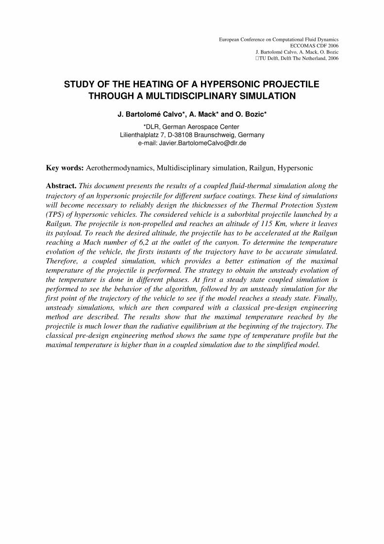
5 RESULTS

At first, a steady state simulation at the first point of the trajectory is performed. Then, anunsteady simulation for the same point is done to verify that the algorithm works by reachingthe steady state temperature. Finally, the evolution of the temperature along the trajectory isobtained and compared with the engineering method.  The first part of the coupled analysisconsists of a steady state simulation for the first point of the trajectory. The structure modelcorresponds  to a  projectile  made of  C/C­SiC.  The same algorithm described  in  Fig.  5   isimplemented, but without the time loop and performing a steady state analysis in the thermalsolver. The algorithm is initialised with a radiative equilibrium solution for an isolated bodyand the iterative process repeated until convergence is achieved. To obtain the solution thetemperature   applied  as   a  BC  in   the  DLR­Tau   solver   is   relaxed   in   order   to   improve   theconvergence of the algorithm: Tfit = wTfit+(1­w)Tfit  , where Tf  is the temperature applied inthe flow solver as BC, and the relaxation factor  to 0,35. The results  of  the algorithm areshown in Table 4. 

Iteration T[K] ∆T[K] q[MW/m2] ∆q[MW/m2] Global residual[%]

RadiativeEquilibrium 2439.04

­1.775

­ ­

Iteration 1 2377.89 61.15 3.302 1.527 1.57E­002

Iteration 2 2356.99 20.9 3.766 0.466 1.61E­002

Iteration 3 2359.50 2.51 3.685 0.081 4.68E­003

Iteration 4 2356.37 3.13 3.767 0.082 5.01E­003

Iteration 5 2358.74 2.37 3.684 0.083 2.27E­003

Iteration 6  2359.83 1.1 3.700 0.016 1.45E­003

Difference 79.79 ­ 1.925 ­ ­

Table 4: Convergence of the solution, steady­state case. 

This   case   is   the  most   restrictive  because   the   temperature   variation   is  quite  high.  Thetemperature difference between the flow solution and the one given by the structural solver inthe first iteration is 200 K, which is a high value. Therefore, the heat flux obtained in the nextiteration is fast two times higher than the radiative equilibrium for an isolated body, and thetemperature has to be relaxed. In the solution process, the temperature at the stagnation pointoscillates   up   to   5­6   iterations   until   it   reaches   its   final   value.  The   chosen   criteria   is   thestagnation point region temperature because the other points of the surface converge withinthe first or second iterations. The converged solution shows that heat flux at the stagnationpoint increases almost a factor 2 while the temperature decreases 3,3% (80 K). The differencebetween both values is due to the extreme conduction of the heat from the stagnation point

J. Bartolomé Calvo, A. Mack, O. Bozic

region, where the heat flux is relatively high in comparison with the other parts of the vehicle.In the unsteady approach no relaxation of the temperature is necessary since the variation

can be controlled assigning properly the time steps. The oscillation is not so high because theelapsed time does not change the temperature so much as in the steady case. For the trajectorysimulations,   the minimum number of  iterations within a given time  interval   is 2.  Here  ispresented also the temperature oscillation between iterations for each time step to show theerror   induced   by   the   algorithm.   The   unsteady   algorithm   is   robust   because   of   the   inneriterations. And, if the obtained heat flux during a time interval is higher than the heat flux ofequilibrium of the iteration, the value of the heat flux during the next time interval will belower than the equilibrium iteration. Thus, if the algorithm does not oscillate, the solution isalways kept under these error estimations. Figure 7 presents of the left side the temperatureand the heat flux of the steady case. On the right side the results of the unsteady simulation forthe first point of the trajectory, as well as the results along the trajectory presented in the nextpoint. The purpose of this simulation is to verify that the unsteady algorithm reproduces thesteady state solution achieving the equilibrium temperature and heat flux. 

Figure 7: a) Steady coupled solution, temperature and heat flux. b) Unsteady results of the first point of thetrajectory. 

The steady simulation with the Whipox material presents the same behavior, but due to thelower thermal conductivity, the equilibrium temperature is near the radiative equilibrium one.The results are summarised in Table 5.

T[K] ∆T[K] q[MW/m2] ∆q[MW/m2]

Radiative equilibrium 2478.74 ­ 1.07 ­

Coupled solution  2455.01 23.74 1.32 0.25

Table 5:  Convergence of the solution, steady­state case. 

J. Bartolomé Calvo, A. Mack, O. Bozic

Finally, the results of the grid convergence study, described in point 3, are presented inTable 6. The conclusion is that all the considered meshes are adapted to solve the problem. 

Fluid/Thermal Ts[K] q[MW/m2] ∆q[MW/m2] ∆Ts[K] єT[%] єq[%]

Fine/Fine 2355.17 3.62 0.00 0.00 0.00 0.00

Fine/coarse 2352.42 3.11 0.51 2.75 0.12 15.00

Stand./Stand. 2360.00 3.50 0.17 4.60 0.20 3.30

Table 6: Convergence of the solution, steady­state case.

5.1 Temperature evolution along the trajectory

To calculate the temperature along the trajectory three flow meshes are used to fasten thecalculation along the trajectory. With the first mesh we calculate the first 4,5 seconds, with thesecond one from 4,5 to 16,5 seconds, and with the third until the end of the simulation. The y+

in   the   stagnation   point   region   is   always   under   0,1.   This   procedure   guarantees   that   theboundary layer, as well as the angle of the shock wave are represented by the flow grid. 

Figure 8: Temperature profiles at the stagnation point over the time. a) Comparison between the coupledmethod, Fay­Riddell, and the radiation adiabatic solution. b) Temperature evolution during the firsts 4 seconds

of the trajectory for both materials.

Figure 8a shows  the evolution  of  the temperature along the trajectory for  the C/C­SiCmaterial.  Three  methods   are   compared,   the   coupled   simulation,   the   radiative   equilibriumtemperature for an isolated body obtained with DLR­Tau, and the pre­design method. Themaximal temperature in the coupled method is reached after 0,76 seconds with a value of1948K, well under the 2439K of the radiative equilibrium temperature at the first point of thetrajectory.   In   the  pre­design  method   the  maximal   temperature   is   also   reached   after   0.76

J. Bartolomé Calvo, A. Mack, O. Bozic

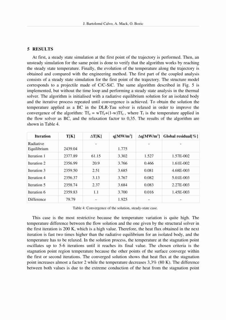
seconds with a value of 2181,8 K. The difference between both maximal   temperatures  is231K and their evolutions are almost parallel over the time. The temperature of the vehicletends to the radiative equilibrium one for an isolated body. As the maximal temperature isreached within the first second of the trajectory and then the evolution is parallel to the oneobtained with  the  pre­design  tool,  only   the first   four  seconds of   the  trajectory have beencalculated for the Whipox material, Fig. 8b. The results are presented on the right hand side ofthe   same   figure.   The   lower   conductivity   and   emissivity   of   Whipox   lead   to   a   highertemperature in the first instants of the trajectory, the temperature reaches a value of 2185 Kafter 0,3 seconds. The pre­design method reaches 2397 K after 0,2 seconds, the difference is212 K. The evolution of both algorithms after  achieving the maximal  temperature is  alsoalmost   parallel.  For   both   materials   the   difference   between   the   pre­design   and   themultidisciplinary solutions is around 200K. 

Figure 9: Temperature profiles along the surface of the vehicle as a function of time for the C/C­SiCmaterial.

The temperature profiles along the surface of the projectile for different time sequences areshown in Fig.9. The temperature is presented as a function of z (see coordinate system in Fig.2b) in order to see better its evolution in the stagnation point region, in the range of 0 to 1,67.During the first second, the temperature overall increases and the profiles are quite parallelbecause not enough time has passed in order to see the effects of the conduction. Then, thetemperature at the stagnation point region reaches it maximum value and the changes betweentime steps are minimal, while the other regions continue to heat up. Then, the temperature atthe stagnation point region decreases while on the other regions continues to increase. It isalso remarkable  the effect  of  the bulk­shell,  which  is  situated near z=6 mm. In  this   timeinterval the effects of the conduction make the temperature raise away from the stagnationpoint region. This express the fact that the dynamic of the temperature is slower in the otherregions   than   in   the   stagnation   point   region.   Finally,   in   Fig.10   the   temperature   field   is

J. Bartolomé Calvo, A. Mack, O. Bozic

presented at two time instants of the trajectory for both materials to its distribution inside thestructure.

Figure 10: a) Temperature inside and on the flow field, t = 1 s. Over: C/C­SiC, under: Whipox. b)Temperature inside and on the flow field, t = 4 s. Over: C/C­SiC, under: Whipox.

5.2 Comments on the pre­design method

The evolution of the temperature for both analytical solutions of the heat diffusion equationlead to the same results in the heating phase, as seen in Fig. 11. The high value of the heatflux and also that not enough time has passed, so that the heat can be transported from thesurface to the inner regions. This constrasts with the phase after the maximum, in which thelength of the slab matters. The lower the thickness of the slab is, the faster cools down thewall. 

Figure 11: Evolution of the temperature, Fay­Riddell method for different wall lenghts compared to thecoupled solution.

J. Bartolomé Calvo, A. Mack, O. Bozic

The differences in the results between both methods are due to the approximations made onthe structural model. On one side, the conduction along the surface is not taken into account ina one­dimensional  model,   this   leads   to  a  higher   temperature  at   the  stagnation  point.  Thesecond point in which the solutions differ is the temperature inside the wall. Indeed, if theprofiles obtained in a fully coupled solution are compared to the ones obtained using the one­dimensional model. The observed difference, Fig.11, is that the temperatures are higher in thecoupled method. Although the temperature at the surface of the vehicle is higher for a pre­design   method,   the   points   inside   the   wall   present   a   lower   temperature   when   we   areconsidering a one­dimensional. This is caused by the neglection of the heat coming form theother parts of the surface to the inner parts of the structure. 

6 CONCLUSIONS

This paper has presented the main differences between a fully coupled simulation and a pre­design   method.   It   is   a   particular   case   of   trajectory,   in   which   the   vehicle   leaves   theelectromagnetic accelerator at  a hypersonic speed,  leading to a very high high flux at  thebeginning of the trajectory. Therefore, an accurate simulation of the first instants of the flightis  needed  to  estimate   the  maximum temperature  reached by   the  vehicle.  The comparisonbetween the coupled and the pre­design methods for different materials show an offset of200K (10,25%) due to the simplifications made in the structural model. The results also show,for   this   type  of   trajectory,   that   the  maximal   temperature   reached by   the  vehicle   is  high,nevertheless it is maintained only during the first few seconds.  

The different material properties and the thermal product characterise the heating of thestructure as it is seen in the results for both materials. Ther thermal product characterises theheating, and the thermal conductivity plays a major role considering the temperature in theinner parts of the strucutre. The higher this value is, the higher the temperatures are inside thestructure. The results show a difference in the order of 500K (25%) between the radiativeequilibrium temperature for an isolated body and the coupled simulation. This is due to theheat conduction during the first seconds of the trajectory, and to the thermal characteristics ofthe material. 

The mass of the TPS in such a vehicle represents a high percentage of the total mass. Thistype of simulation enables a better estimation of the temperatures at the surface and inside thevehicle. Thus, the thicknesses of the outer layer as well as the insulation layer can be betterdesigned. For this trajectory, the differences between the approaches are high, the radiativeequilibrium temperature and the maximal obtained with a coupled simulation differ in a 25%.Thus, the calculation of the thicknesses between the approaches are to take into account. 

7  ACKNOWLEDGEMENTS

The authors of the paper would like to thank J.M Longo for his help and advice during therealisation of this work.  

J. Bartolomé Calvo, A. Mack, O. Bozic

REFERENCES

[1]   J. Behrens, P. Lehmann, J. Longo, O.Bozic, M. Rapp, and A. Conde Reis, Hypersonicand   Electromagnetic   Railgun   technology   as   a   future   alternative   for   the   launch   ofsuborbital   payloads,  16th   ESA   Symposium   on   Rocket   and   Balloon   Programmes,   St.Gallen (CH), (2003).

[2]   O. Bozic, J.M. Longo, P. Giese, and J. Behrens, High­end concept based on hypersonictwo­stage rocket and electromagnetic railgun to launch micro­satellites into low­earth­orbit,  Fifth European Symposium on Aerothermodynamics for space vehicles, Cologne(2004). 

[3]  H.  Hald,  Operational   limits   for   reusable  space  transportation  systems due   to  physicalboundaries of C/SiC materials, Aerspace Science and Technology, 7, 551­559 (2003).

[4] H. Schneider,  M. Schmücker,  J.  Göring,  Kanka B., She S.,  and Mechnich P,  PorouseAlumino Silicate Fiber/Mullite Matrix Composites: Fabrication and Properties,  Ceram.Trans., Vol. 115, Westerville, OH: Am. Ceram. Soc.  (2000). 

[5] R.  D. Quinn,  L. Gong,  A Method for Calculating Transient  Surface Temperature andSurface Heating Rates for High­Speed Aircraft, NASA TP 2000­209034 (2000).

[6] F. Seiler, U. Werner, G. Patz, Ground Testing Facility for Modeling Real Projectile FlightHeating in  Earth Atmosphere,  Journal of  Thermophysics and Heat Transfer,  Vol. 16,No.1, 101­108 (2002).

[7] A. Mack, V. Hannemann, Validation of the Unstructured DLR­TAU­Code for HypersonicFlows, AIAA Paper 2002­3111 (2002).  

[8] John  D.  Anderson,  Hypersonic   and  High  Temperature  Gas  Dynamics,  McGraw­HillSeries on Aeronautical and Space Engineering, New York 1989.

[9]  A.  Mack,  R.  Schäfer,   Fluid   Structure   Interaction   on   a   Generic  Body­Flap   Model   inHypersonic Flow, Jounal of Spacecraft and Rockets, Vol. 42, No. 5 (2005).

[10]  R. Schäfer, A. Mack, E. Burkard, and A. Gülhan, Fluid­Strcture interaction on a genericmodel of a reentry vehicle nosecap,  ICTS 5th  congress on thermal stresses and relatedtopics, Blacksburg, Virginia, USA 2003.

[11]  R. Savino, M. De Stefano Fumo, D. Paterna, M. Serpico, Aerothermodynamic study ofUHTC­based thermal protection systems, Aerospace Science and Technology, 9, 151­160(2005). 

[12] F. Infed, F. Olawosky, and M. Ausweter­Kurtz, Stationary Coupling of 3D HypersonicNonequilibrium   Flows   and   TPS   Structure   with   Uranus,  Journal   of   Spacecraft   andRockets, Vol. 42, 0022­4650 (2005).

[13] N. Billiard, V. Iliopoulouv, F. Ferrara,   R. Denos, Data reduction and thermal product

J. Bartolomé Calvo, A. Mack, O. Bozic

determination for single and multi layered substrates thin film gauges, 16th Symposium onMeasuring Techniques in transonic and supersonic flow in cascades and turbomachines,Cambridge, United Kingdom (2002).

[14] H. Julian  Allen, A. J. Eggers Jr., A Study of the Motion and Aerodynamic Heating ofBallistic Missiles Entering the Earth's Atmosphere at  High Supersonic Speeds,  NACATechnical  Report  1381, Forty­Fourth Annual Report  of   the NACA,  Washington,  D.C.(1959).