STUDY OF SYNTHETIC APERTURE RADAR (SAR) … · (SAP.) I8?,GSfy CHA-.ACTEFISTICS ... theoretical analysis consists of enumerating the known sources contributing to geometric ... steady-state

:eooCM

ecIU

O

7 ( N A S A - C F ~ 1 « 1 3 9 8 )I A P 2 P T U 5 E F A D A P (

S T U D Y O F S Y N T H E T I C(SAP. ) I8? ,GSfy C H A - . A C T E F I S T I C S

Final Repor t (Goody-ear Aerospace Corp . )83 p HC Sii.75 CSCL 171

G3/32Unclas26U25

STUDY OF SYNTHETIC APERTURERADAR (SAR) IMAGERY CHARACTERISTICS

CONTRACT NO. NAS 6-2571

; : SUBMITTED TO ":

NATIONAL AERONAUTICS AND SPACE ADMINISTRATION

WALLOPS STATIONWALLOPS ISLAND, VIRGINIA

GERA-2089

30 MAY 1975

ARIZONA DIVISION '•

AEROSPACE CORPORATION• • VlTCHFIELD PARK, ARIZONA

https://ntrs.nasa.gov/search.jsp?R=19750016924 2018-08-25T20:30:28+00:00Z

GOODYEAR AEROSPACECORPORATION

ARIZONA DIVISION

STUDY OF SYNTHETIC APERTURE RADAR

(SAR) IMAGERY CHARACTERISTICS

Contract No. NAS 6-2571

Submitted to

National Aeronautics and Space AdministrationWallops Station

Wallops Island, Virginia

GERA-2089 30 May 1975Code 99696

4779

GERA-2089

ABSTRACT

This is the final report to NASA Contract NAS 6-2571.

Sources of geometric and radiometric fidelity errors in

AN/APQ-102A radar imagery are discussed, along with a

digital computer program to correct the distortions. The

major effort, a computer program which will process

digitalized recorded AN/APQ-102A phase histories into

imagery, is described. All computer programs are listed.

-iii-

GERA-2089

TABLE OF CONTENTS

I INTRODUCTION

LIST OF ILLUSTRATIONS vii

Section Title

H DEFINITION OF IMAGERY CHARACTERISTICS 3

1. General . 3

2. Geometric Fidelity Analysis 3

3. Across-Track Errors 4a. Ground Range Sweeps 4b. Film Thickness Variations 4c_. Range Displacement Error from Target Altitude 4

4. Along-Track Error 5a. Recorder Film Drive Error 5b. Film Thickness Variations 6c. Clutterlock Stability 6d. Correlator Film Drive Error for Optically Processed

Imagery -t 6e. Residual Error from Motion Compensation

Instrumentation 7i. Effect of Clutterlock and Across-Track Velocity

Measurement Error 9g. Effect of Vertical Velocity Measurement Error 9h. Effect of Vertical Velocity Measurement Error 10j. Antenna Pitch and Yaw Errors . 11_i. Aircraft Turning Error 13

5. Measurement of Geometric Errors 14a. General 14b. Program Rationale 15c_. Program Steps 15d_. Program Parameters 18

^ e. Results 19

TABLE OF CONTENTS G ERA-2 089

Section Title

6. Radiometric Errorsa. Generalb. Sensitivity Time Control (STC)c_. Antenna Illumination . . . .

III DIGITAL PROCESSING OF IMAGERY

1. Digital Azimuth Processing . . .

2. Removal of Image Skew

3. Scale Factor Correction . . . .

IV CONCLUSIONS

Appendix

A TARGET SIMULATOR . . . . . . .

B AZIMUTH PROCESSING

C DISTORTION ANALYSIS ,

D IMAGE DISTORTION CORRECTION . ,

19191920

23

23

36

39

41

A-l

B-l

C-l

D-l

-vi-

GERA-2089

Figure

1

2

3

4

5

6

7

8

9

10

LIST OK n,l,USTHATK)NS

Title

Geometry and Motion Compensation Error .

Geometry of Antenna Pitch and Yaw Error

Geometry of Errors Resulting from Uncompensated Turn . . . . .

Theoretical Vertical Antenna Pattern at Horizontal Boresite . . .

Digital Processing of SAR Data - Flow Diagram

Antenna Azimuth Frequency Response

Format of Data after Skew Correction .

Placement of Zero Data Points

Page

8

11

13

21

24

28

30

38

38

39

-vii-

GERA-2080

SECTION I - INTRODUCTION AND SUMMARY

This report describes the work accomplished on a study program entitled, "Study of

Synthetic Aperture Radar Imagery Characteristics," funded under NASA Contract NAS 6-2571.

The objective of the program was to analyze the characteristics of synthetic aperture radar

(SAR) imagery and develop digital processing techniques to utilize this type of data in con-

junction with other sensor data on the NASA earth resources program. Specifically, the

major effort was directed toward producing the digital computer programs for the processing

of data obtained from the AN/APQ-102A radar system.

The study program consisted of two major tasks: (1) the definition of SAR image character-

istics, and (2) the development of digital computer programs to accept phase history data and

generate a radar image normalized relative to both intensity and geometry.

Section II discusses the sources and magnitude of errors in the AN/APQ-102A imagery. The

theoretical analysis consists of enumerating the known sources contributing to geometric

distortion, determining the effect of each source, and combining to yield an overall estimate

of the geometric fidelity of the imagery. Sources for geometric distortion fall into three

categories: (1) sensing geometry, (2) radar equipment errors, and (3) errors in the aircraft

inertial navigation system (INS) and altimeter. In addition to the theoretical analysis, the

distortions in an AN/APQ-102A image of Wallops Island flown on 30 August 1973 were

measured.

Section III describes the computer programs and procedures developed to process AN/APQ-

102A phase history data. These programs and procedures were validated by actually

processing imagery at the Wallops Station facility utilizing the Optronics Microdensitometer

and the Honeywell 625 computer. This validation effort included the training of Wallops

Station personnel, thus giving NASA the capability to process subsequent radar data without

contractor support.

Conclusions are given in Section IV, and the appendixes contain program listings of all

computer programs generated or used.

-1-

GERA-2080

SECTION II - DEFINITION OF IMAGERY CHARACTERISTICS

1. GENERAL

The AN/APQ-102A has been quite successful in mapping for tactical purposes; however,

its imagery has small geometric and radiometric fidelity errors which it would be

desirable to remove when it is being used for cataloging earth resources. Some of the

geometric errors are internally generated within the radar; however, these errors are

generally small. The major sources of geometric errors are inertial system errors.

Since these errors are not known for any particular flight, their effect (geometric dis-

tortion) must be measured by comparison with a map or other well-controlled data. This

section discusses the error sources, their effect on geometric fidelity, and a method of

measuring geometric distortions through the use of terrain features recognizable both in

the radar image and on a map.

The basic design of the AN/APQ-102A includes features that minimize radiometric dis-2 1/2tortions that would be caused by sensing geometry (£.£., esc cos vertical antenna

pattern). Radiometric distortions can be determined by measuring the deviation of the

radar transfer function from the ideal or by imaging a calibrated radiometric range.

Only the first of these methods is discussed.

2. GEOMETRIC FIDELITY ANALYSIS

The velocity and flight characteristics of the RF-4 aircraft and its avionics are used in

the numerical calculation of the magnitude of the error components. The calculation is

typical of the parameters of the flight of 30 August 1973. This analysis includes only

fixed target imagery and only the modes listed in Table I.

PRECEDING PAGE BLANK

-3-

SECTION II GERA-2080

TABLE I -AN/APQ-102A HIGH-RESOLUTION OPERATING MODES

Mode

1

5

6

7

Altitude(ft)

500 to 5, 000

30,000 to 50,000

30,000 to 50,000

30,000 to 50,000

Type ofcoverage

HR

HR

HR

HR

Range coverage(NMI)

0 to 10 both sides

5 to 15 both sides

10 to 30 left

10 to 30 right

Velocity(ft/s)

700 to 1250

700 to 2000

700 to 2000

700 to 2000

3. ACROSS-TRACK ERRORS

a. Ground Range Sweeps

The CRT recorder in the AN/APQ-102A employs ground range sweeps. Two

characteristics of the sweep are normally considered relative to geometric fidelity,

i_.e_., linearity and stability. Sweep linearity is expressed in terms of percent error

in the distance between two points in the sweep interval. The linearity of the sweep

of the AN/APQ-102A is ±0.5 percent. The error in position of a target at one edge

of the swath with respect to the other for a 10-NMI swath is

±(0.005) X (5) (6080) = ±152 ft (1)

The long-term stability of this error should be good, and the error should be highly

correlated between data films using the same recorder on successive missions.

The expected dominant spatial frequency of this range scale factor error is one-half

cycle per sweep length, with the error near the center of the sweep trace being very

small.

b_. Film Thickness Variations

Linear film thickness variations can cause errors on the order of four feet in the

range direction. The spatial frequencies of these errors have not been determined.

-4-


c_. Range Displacement Error from Target Altitude

Conversion from slant range measurement to ground range measurement depends on

the relative altitude between the radar flightpath and a given target and thus is

affected by terrain roughness, earth curvature, etc. No error is attributed to the

radar for this operation.

4. ALONG-TRACK ERRORS

a_. Recorder Film Drive Error

The major error in film drive is caused by the error in the measurement of ground -

speed. The accuracy of the velocity measuring equipment is about nine feet per

second. Thus, the linear error in target location resulting from errors in velocity

is

VE

EV = V~ X D ' (2)Y

where

V = error in velocityiLi

V = aircraft velocity

D = the along-track distance over which error is to be considered.

In a high-speed mode over a five-mile distance, the linear error is

x 5 x 608° = 18° ft • (3)

It can be further assumed that a three-mil peak sinusoidal error is present because

of eccentricity of the film metering drum. This would be equivalent to a three-foot

error.

-5-

SECTION II . GERA-2080

b_. Film Thickness Variations

The errors from film thickness variations are estimated to be small (about four feet).

£. Clutterlock Stability

The stability of the clutterlock motion compensation loop is about five Hertz and

would produce an error in the longitudinal (y) direction according to the following

relationship:

d f Xd (4)

n | 2 Vy

where

frequency error - df - 5 Hz

wavelength '= X - 0.1 ft

groundspeed = V • = 1500 ft/s

•E =. relative error

£ = fTO — T? ^min max 2V

y

30.400 X 5 X 0. I '... 2 X 1500 " ° U '

This is a skew-type error, and its frequency is estimated to be very low.

d_. Correlator Film Drive Error for Optically Processed Imagery

Aspect ratio error contributes a small, steady-state error in the image azimuth

scale factor. This error is held to less than a resolvable element and is estimated

-6-


to be 15 feet. Data film drive error resulting from metering drum eccentricity is

the same as that of the recorder and is three feet. The image fi lm metering drum

eccentricity permits a maximum sinusoidal error of 23 feet peak at a period of

3.9 NMI.

e. Residual Error from Motion Compensation Instrumentation

Compensation for sideways motion in the AN/APQ-102A radar is achieved in the

following manner. An antenna-mounted accelerometer system measures the side-

ways accelerations which are integrated and combined with the clutterlock-

measured velocities. The clutterlock takes an average of range samples at intervals

along the entire 10-mile swath. Hie motion compensation signal thus derived is

applied at midrange. Thus, no along-track error exists at this point; however, an

error does exist on each side of the midpoint, with maximum error at maximum

and minimum ranges.

To obtain an expression for this error, consider a velocity in the X direction, V .X

A correction is made so that no error exists at Y . However, there is a differenceobetween the hyperbola on which mapping is occurring and the straightline correction

that is applied. From Figure 1, the following expressions may be written:

1/92 o i/"Y = (R H h") cos 0 (5)

VX 2 2V R

0 = (KO + li ) cos 0 (8)

-7-


cos1/2

<R

(9)

VX

R

V1/2 Vy o

2 2+ h

1/2 2 22 2

_

V(10)

The along-track error is

1/2

Y - Y = —0 V, 1/2

1/2

R - R° 2 2 1/2

<R2o + h2) .

V. (11)

4779-2

Figure 1 - Geometry and Motion Compensation Error

-8-


If the velocity, V , is 10 ft/s, V is 1500 ft/s, R is 20 miles, R is 15 miles, andX Y O

h is 40,000 ft, the error is

Y - Y, = 26.7 ft (12)

_f. Effect of Clutterlock and Across-Track Velocity Measurement Error

An across-track velocity measurement error introduces a squint or skew into the

final image. An across-track velocity measurement error of 6 ft/s at 1500 ft/s

produces a pointing error of

ANGULAR = 4 X 10~3 radian(13)

The linear error along track of a target on one edge of the swath with respect to the

other is

AVX

'CTV V (RMAX " RMIN)

1500(10) (6080)

- 243 ft (14)

Effect of Vertical Velocity Measurement Error

An expression relating vertical velocity to along-trnck error can be developed

similar to that for across-track velocity:

V.

V.evv = h

2

2

2 1/2 -

h2,172 "(15)

-9-


For the conditions M

V = 3.5 ft/s . -

V = 1500 ft/s

h = 40,000 ft

R = 20 NMI f:

R = 15 NMI ;o

therefore,

T?

h_. Effect of Vertical Velocity Measurement Error

The along-track effect of vertical velocity measurement error may be determined

from the expression

eAV = rp X AVZ Vy Z

For the parameters

AVZ = 2 ft/s

V = 1500 ft/s

h =• 40, 000 ft ,

the along-track error resulting from vertical velocity measurement error is

£AVz - *2

L?

-10-


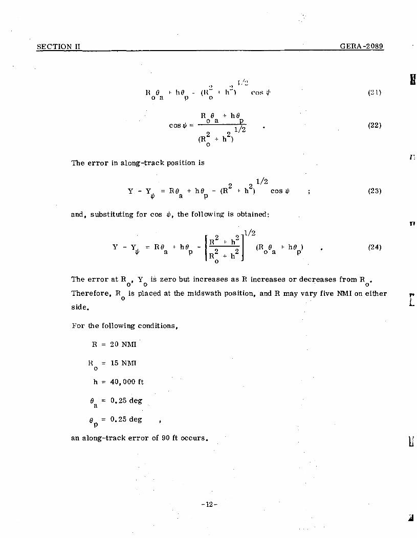
Antenna Pitch and Yaw Errors

Errors in antenna pitch and yaw will affect along-track geometric fidelity. The

result is that the clutterlock attempts to correct for the error, causing a skew in

the imagery. Consider the geometry of Figure 2. The aircraft is flying at velocity

with an antenna pitch of 6 and yaw of 6 . The error in the along-track direction isp a

the mismatch between the best-fit doppler line and the antenna pattern intersecting

the ground. This error is Y - Y. .

From Figure 2, the following expressions may be written:

„ „ 1/2Y - (I

Y = R0

Y = R e +o o a

COS ill (18)

(19)

(20)

4779-3

Figure 2 - Geometry of Antenna Pitch and Yaw Error

-11-


H O i h 0o a p

ID ros 4> (21)

cos il> =E e *- he

o a p1/2

(22)

The error in along-track position is

1/22 2Y - Y = Ee + h0 - (R + h ) cos

$ a p

and, substituting for cos il>, the following is obtained:

(23)

Y - Y, - E9 > h0 -4> a p

9 9R" H h"

2 9R + h"

O J

«./ ^>

(R 0 »-o a

(24)

The error at R , Y is zero but increases as R increases or decreases from R .o o oTherefore, R is placed at the midswath position, and R may vary five NMI on either

side.

For the following conditions,

R = 20 NMI

R - 15 NMIo

h = 40, 000 ft

9 = 0 . 2 5 deg3.

e = 0 . 2 5 degP

an along-track error of 90 ft occurs.

-12-


j. Aircraft Turning Error

The inability of the aircraft to fly a perfectly straight path introduces errors in the

along-track direction. When the aircraft goes into a slow turn within the time con-

stants of the clutterlock, the clutterlock is able to keep the physical beam oriented

on the zero doppler line. However, the radar thinks it is following a straight line

flightpath and, as a result, the imagery is skewed. The geometry of this situation

is depicted in Figure 3. Here, r is the uncompensated turning radius of the aircraft,

R is the range of interest of the radar, s is the length of the ground track in rotating

through the angle 8, and S is the distorted, recorded length of the flightpath. The

error caused by the aircraft turn may be written as

S - ss

(r ^ R)0 - rg Rr (25)

4779-4

Figure 3 - Geometry of Errors Resulting from Uncompensated Turn

-13-


It is di f f icul t to determine what the minimum uncompcnsnted turning radius for the

HF-4 or C-54 is, but the manufacturer of the R\'-4 has indicated that it wil l fly

straight with a minimum turn radius of 2G50 NMI. Therefore, the error resulting

from a turn expressed in percent is

•p in€T = r 2650 = 0'00378 = °'38 Percent • (26)

When one considers a strip five NMI long, the turning error is

e = (0.0038) X 5 X 6080 - 115 ft .

5. MEASUREMENT OF GEOMETRIC ERRORS

a_. General

It can be seen from the foregoing that most of the fidelity errors are random and

are irreducible prior to imaging, because they represent the utilization of onboard

sensors and their attendant errors. Certain errors such as residual motion compen-

sation error and the skew introduced by use of an offset frequency for demodulation

could be removed after flight if the offset frequency and the three-axis translation

of the aircraft were recorded during flight. These data, however, are not available

in the AN/APQ-102A, and hence the aforementioned errors are not separable from

the random errors.

As a postflight procedure, the processed radar image may be rectified by use of a

computer program which does a least-square-error fit using precisely imaged

points whose geographic corrdinates are accurately known. Care must be taken that

points utilized are coincident with the points whose coordinates are known.

-14-

SECTION n ; _ GERA-2089

b.

For the distribution correction program, the following radar image distortions were

considered:

1. Scale (range versus track) - caused by the separate scaling

mechanisms involved (in the radar) in the track and range

directions

2. Skew - caused by either radar antenna or correlator slit

misalignment (results in range and track nonorthogonality).

3. Residual distortion - that which remains after items 1. and 2.

have been accounted for (caused by height differences between

the radar ground plane and the elevation of objects in the ground

area being imaged, nonlinearities in the recording CRT,

measurement errors, etc.).

c_. Program Steps

Since the program determines the distortion relative to (radar) range and track,

a prerequisite for the analysis is that the radar image measurements (of identified

ground control points) be performed with the X-axis of the measurement device

aligned with the track direction of the radar. The steps taken by the program in

analyzing distortion are summarized as follows:

1. The ground coordinates of the control points are preliminarily

aligned with the image coordinate system. This is done by

determining the relative orientation of two designated control

points in both the image and ground frames and rotating the

ground system to coincidence. For correctly signed printout

of scale, skew, and distortion, it is desirable to choose the

ground axes to lie within 45 degrees of the image coordinate

-15-


system (for an existing system, (his is neeomplishetl by

controlling the sign and (X-Y) designation of the axes). The

designation of alignment points (as a program parameter)

prevents the use of points known to have a high probability of

substantial relative distortion (e_.g., points extremely close

together). The selection of two widely spaced points will

suffice for the initial alignment

2. A least-squares fit between image and ground range coordi-

ates is performed. The range errors remaining after the fit

are computed, and the linear correlation coeffficient between

range errors and track coordinates is determined (if a nonzero

coefficient exists, it indicates a residual misalignment). The

ground coordinates are then rotated to make the coefficient

zero. This process prevents individual control point errors

from introducing substantial alignment errors

3. A least-squares fit between the range image and ground

coordinates is computed and residual errors determined

(at ground scale)

4. Track image and ground coordinates are scaled via a least-

squares fit and average error determined. Skew is then

introduced into the image coordinate system via two equations:

Y' = Y (27)

and

x'(I) = X(I) + A • Y(I) , (28)

II

-16-

SECTION II • GKHA-2089

where

(X, Y) = original image coordinatesi r

(X ,Y ) = skewed coordinates

A = tangent of skew angle.

The skew angle is varied (in sign and magnitude) until track

errors are minimized (as measured by successive least-

squares fits)

5. Several types of analyses are then performed by the program

to demonstrate the relative contribution of various error

sources. In each of them, the residual error variance and

individual point errors (ground scale) are computed (and

displayed for examination) after various types of image

correction are introduced. The four types of correction are:

a. A magnification equal to the average (range and

track) scaling difference between image and

ground coordinates

b. Differential scale correction

c. Magni l ' i rn l ion plus skew cm-reel ion

d. Differential scale and skew correction.

The image range scale, track scale, and skew are displayed.

Plots are created (using CalComp software) which illustrate

the ground position and residual error of the control points

after the various types of correction.

-17-

SKCTION II GKHA-2089

d_. Program Parameters

The program listing is given in Appendix A. 'Hie utilization of the results to

restitute digitally processed imagery is discussed in Section III.

Program parameters are as follows:

ALPHA 1 - ALPHA 4 Analysis section headers

N

Nl, N2

SCPLT

SCERR

A (I)

Number of control points

Number (corresponding to program

order) of point pair to be used for

initial alignment. Nl and N2 should

be ordered so that Nl has a smaller

track coordinate than N2 (however,

Nl < N2 need not be true; Ue_.,

control points may be entered in

any order)

Scale of plots (ground units/inch)

which are created of control point

positions

Scale of error vectors

Ground coordinates of control point

Image coordinates of Ith control point

Alphanumeric control point

designator.

SECTION II GKRA-2089

(J. Results

A section of the AN/APQ-102 data film which was flown for NASA on the 30 August

1973 flight was optically correlated on a laboratory correlator, and the portion of

the imagery around Wallops Island was analyzed. Sixteen points were used, of

which coordinates for 6 were from triangulation and 10 from a map. After distor-

tion correction, the mean error along track was zero with a standard deviation of

77.52 meters and mean across-track error of 7.2 meters, with a standard

deviation of 87.7 meters.

6. RADIOMETRIC ERRORS

a. General

As mentioned previously, the transfer function of the AN/APQ-102A was designed

to compensate for sensing geometry, ideally resulting in no radiometric distortion.

To the extent that the radar transmitted power and the receiver gain remain constant

(this can be accomplished by disabling the automatic gain control), the radar can be

designed to compensate for changes in slant range and depression angle. These

compensations are accomplished with sensitivity time control and a vertical antenna

pattern designed for uniform illumination as a function of depression angle.

Deviations (from the ideal) of these functions can cause rndiometric errors.

b. Sensitivity Time Control (ST(')

Reference 1 contains instructions on how to adjust the STC'to give the desired

signal. This description includes wave shapes and is considered the best data

available. The STC so adjusted requires no correction. The STC is turned off in

modes used above 30, 000-ft altitude and does not apply to the flight of 30 August 1973.

SUSAF T.O. 12P3-2APQ102-2-4. Radar Mapping Set, AN/APQ-102 and AN/APQ-102A(Frequency Converter-Transmitter CV 1678/APQ102), Chapter 11.

-19-

SECTION II CERA-2089

'

»_. „

It can be shown that if the vertical antenna pattern has a gain

2 1 / 2G = K esc 0 cos 0 , (29)

then the terrain would be uniformly illuminated as a function of depression angle 0.

/Such a pattern can be synthesized over a limited angle. In the AN/APQ-102A, the

pattern is normalized at 18 deg. Figure 4 shows the theoretical vertical antenna

pattern of the AN/APQ-102A, together with the tolerances in gain. The standard

deviation of the one-way gain from uniform illumination is less than 0.5 dB. The

antenna pattern of the arrays to be used can be measured and the deviation between2 1/2measured values and the ideal esc" fl cos ' " 0 determined. It was anticipated that

the measured antenna pattern could be used to make radiometric corrections to the

imagery of Wallops Island made on 30 August 1973. However, it has been deter-

mined that USAF records do not make this possible. Therefore, no corrections for

the antenna pattern were made. The image distortion program discussed in

Section III has such provisions.

U

-20-

SECTION n OKI? A -2089

Figure 4 - Theoretical Vertical Antenna Pattern at Horizontal Boresite

-21-

GKHA-20S!)

SECTION III - DIGITAL PUOCKSSINC. OK IMAGKHY

1. DIGITAL AZIMUTH PROCESSING

The processing described in this section will accommodate AN/APQ-102 radar data

which has been range compressed, recorded optically, scanned, and digitized for

processing. The azimuth compression will be performed by a high-speed digital com-

puter. The data flow diagram is given in Figure 5. The processing will be performed

to obtain 30-ft-resolution imagery with the option of either one or two azimuth looks.

If more rapid processing of the data is desired, the azimuth resolution may be degraded.

The data will be processed for an azimuth offset that is nominally PRF/4. In actuality,

the azimuth offset frequency is not exactly known, and the data processing must take

this into account. To maintain low sidelobe levels, an oversampling factor of at least

four will always be maintained. The sampling rate of the input data will be not be

reduced until azimuth compression is being performed.

The implications of the foregoing may be better understood by examining the fundamental

formulas for azimuth compression. The synthetic aperture length which must be flown

to attain a desired 3-dB azimuth resolution, W , is

0. 8 8 A H ,LSYN = ~^T~ ' <:'°>

A

where R is the slant range to the target measured on a line perpendicular to the flight-spath, and X is the wavelength of the transmitted signal.

However, when the phase history of a point target which has been collected over the

required L N is compressed (i.e_., processed in a matched filter), the resultant side-

lobes of the sin (x)/x compressed waveform have a -13.6-dB peak and decay slowly.

-23--

SECTION III GERA-2089

WISSTO

5

IPS

^

>F /

'

,

AZIMUTH

PROCESSING

PROGRAM

OUTPUT TO BEVISUALLYI NED AND COM-PARISONS HADE

Figure 5 - Digital Processing of SAR Data-Flow Diagram (Sheet 1 of 2)

-24-


( INPUT DATA [

"" J

GROUND RANGE

RADAR DISTORTION

ANALYSIS PROGRAM

CARD

INPUT

PRINTEDOUTPUTn,.—> TEST TAPE

GENERATOR

IHAGE DISTORTION

CORRECTION

PROGRAM

1'MICRO-nruc 1 .

TOMETER

ORIGINAL PAGE ISOF POOR QUALITY

Figure 5 - Digital Processing of SAR Data-Flow Diagram (Sheet 2 of 2)

-25-

SECTION III • GERA-2 089

These sidelobes present a problem in that the sidelobes of a large target may have

larger amplitudes than the mainlobe of a target, and hence mask it. To prevent this

from occurring, a weighting function is applied to the return phase history. Basically,

the weighting function reduces the sidelobes by the application of a symmetrical taper

across the azimuth phase history of a target. This symmetrical attenuation, however,

causes a broadening of the mainlobe of the target when azimuth compression is per-

formed. To maintain the desired resolution, yet achieve a low sidelobe level, excess

azimuth bandwidth is required.

Typical of the weighting functions which may be applied are Taylor aperture functions.

A Taylor aperture function which suppresses the peak sidelobe to -30 dB will broaden

a point target's mainlobe by a factor of 1.42. When this weighting function is used,

_ 1.25XRLSYN ~

Processing is being performed for a finer resolution than is specified, with the know-

ledge that the weighting function is being utilized and will broaden the mainlobe to that

desired.

If the antenna's real azimuth beamwidth, /?, (here considered to be 3-dB beamwidth) is

capable of illuminating more azimuth extent than is required for a desired resolution,

i_.e_. , if

V > T ' S Y N ' <32)

then the excess illuminated area may be used to form more than one synthetic aperture.

For the AN/APQ-102A system, the 2-way 3-dB beamwidth is approximately 1 degree,

which would theoretically imply that 8 synthetic apertures for 30-foot resolution exist

between the 3-dB points of the antenna beam:

R ( ldeg ) /KXR

— •

-26-

SECTION HI GERA-2089

However, because the limitations of the motion compensation INS, azimuth recorder

bandwidth, etc., blurring of the image will possibly occur if more than two looks are

combined. Thus, for this problem,

_0

L M = 2.083 X 10 X R x number of looks , (34)oi IN S

where L is the synthetic aperture length in feet, R is the slant range in feet, andox .W

the number of looks is either one or two.

The AN/APQ-102 radar has a PRF of 1.1 V, where V is the aircraft velocity in feet per

second. Therefore, a sample of the terrain is collected once per 0.9091 ft of aircraft

travel. This sampling is greatly in excess of that necessary for 30-ft resolution, which

is

30minimal sample spacing = ——— ft . (35)

2 X 1.25 X number of looks v '

(The factor of 1.25 in the denominator accounts for me excess bandwidth required to

preserve resolution when using the weighting function.) It is necessary to have this high

PRF to keep the spectrum which lies within the antenna's mainbeam unambiguous.

The unambiguous bandwidth of the sampled spectrum lies from zero frequency to 1/2

PRF, or 0.55 cycle/ft. The clutterlock, however, keeps the antenna, and hence the

doppler spectrum within its mainlobe, centered on zero doppler. Therefore, it is neces-

sary to translate the return mainlobe spectrum up in frequency so that a frequency of

-0.275 cycle/ft will He at zero frequency, and a frequency of ^0.275 cycle/ft will lie at

0.55 cycle/ft. This is accomplished by mixing the return with an azimuth offset fre-

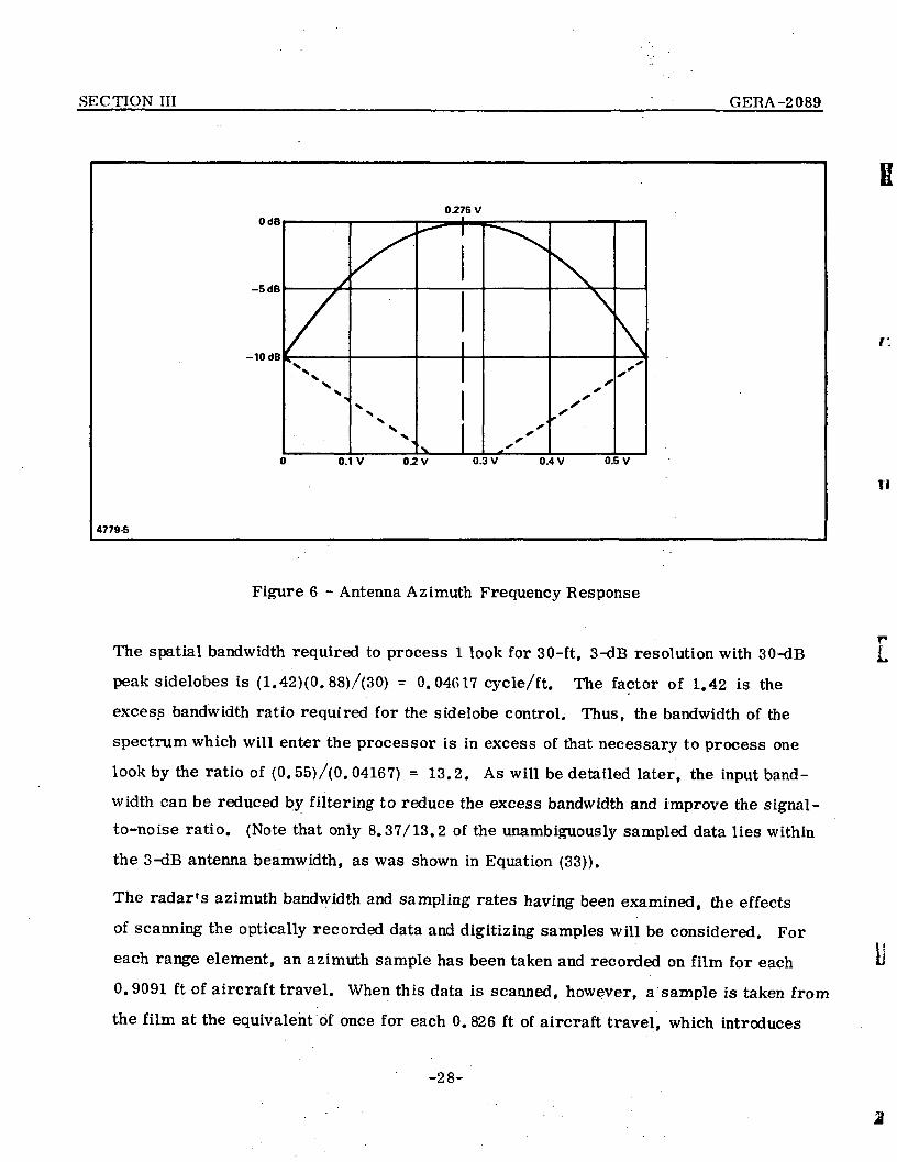
quency of 1/4 PRF. The translated return spectrum is illustrated in Figure 5. Energy

at frequencies above ±0.275 cycle/ft will fold back into the spectrum of interest.

However, as is illustrated by the dashed lines in Figure 6, this energy is heavily

attenuated by the rolloff of the antenna's mainlobe. The peak sidelobes of the AN/APQ-

102A 2-way antenna pattern are more than 26 dB down, and thus the energy in them will

contribute little to the processing noise.

-27-


0.275 VOdBi

-5dB

-10 dB

0.1 V 0.2 V 0.3V 0.4V 0.5V

4779-5

Figure 6 - Antenna Azimuth Frequency Response

The spatial bandwidth required to process 1 look for 30-ft, 3-dB resolution with 30-dB

peak sidelobes is (1.42)(0. 88)/(30) - 0.04617 cycle/ft. The factor of 1.42 is the

excess bandwidth ratio required for the sidelobe control. Thus, the bandwidth of the

spectrum which will enter the processor is in excess of that necessary to process one

look by the ratio of (0.55)7(0.04167) = 13.2. As will be detailed later, the input band-

width can be reduced by filtering to reduce the excess bandwidth and improve the signal-

to-noise ratio. (Note that only 8.37/13.2 of the unambiguously sampled data lies within

the 3-dB antenna beamwidth, as was shown in Equation (33)).

The radar»s azimuth bandwidth and sampling rates having been examined, the effects

of scanning the optically recorded data and digitizing samples will be considered. For

each range element, an azimuth sample has been taken and recorded on film for each

0.9091 ft of aircraft travel. When this data is scanned, however, a sample is taken from

the film at the equivalent of once for each 0. 826 ft of aircraft travel, which introduces

-28-

SECTION in GERA-2089

an effective increase in the azimuth sampling of a factor of 1.10. It must be understood

that no increase in the information bandwidth has occurred, that having been restricted

by the original PRF. However, there is a translation of all frequencies because of the

resampling. All data must be treated as though the spatial bandwidth were (0. 55)(1.1) =

0.605 cycle/ft, even though no information lies in the portion of the unambiguous spec-

trum resulting from the different input and output data rates.

The digitized data will be treated as if the original PRF produced a factor of (13.2)(1.1) =

14.52 in excess bandwidth over that required for a single azimuth look. Each azimuth

look will thus occupy (0.04167/0.605) X 100 = 6 . 9 percent of the unambiguous sampled

bandwidth.

The first operation in the digital processing of the data is to bandpass only those

frequencies necessary for azimuth compression, and thereby improve the signal-to-noise

ratio by reducing the noise bandwidth. T/his is done in the azimuth prefilter, which has

been designed (described below) to have a nominal center frequency of 0.4545 (i.e_.,

PRF/4/1.1) of the sampled bandwidth and have 0. 04167 and 0.08334 cycle/ft spatial

bandwidths for the one- and two-look cases, respectively.o

The two azimuth prefilter functions are "window function" designs. To produce a

window function with a desired center frequency and bandwidth, the following procedure

is employed (the steps are illustrated in Figure 7):

1. In the frequency domain, place an i in pulse at the desired fraction of

the bandwidth for which the filter's center frequency is to lie, and at

the corresponding negative frequency

2. Take the inverse discrete Fourier transform (IDFT) of this spectrum.

The result will be a sampled cosine in the time domain having an

integer number of cycles over the time extent of the IDFT output

Q . .

Gold, B. and Rader, C.M.: Digital Processing of Signals. McGraw-Hill, 1969, pp. 217-231.

-29-

SECTION HI GERA-2089

4779-6

STEP1

AMPLITUDE

I—-'MAX

-f-) FREQUENCY

'MAX

STEP 2

4. +

4 4 4 - 4

SAMPLED COSINE

• TIME1

T = 04 4 4 4 - 4 - 4 -

+ » 4 4

MAX

STEPS WEIGHTING FUNCTION ENVELOPE

T= :

T = 0SAMPLED WEIGHTEDCOSINE

STEP 4

AMPLITUDE

A FREQUENCY

-fMAX-f

'MAX

Figure 7 - Window Filter Design

-30-

SECTION III _ . _ GERA-2089

3. A weighting function, in this case, a 40-dB Taylor function, is point

by point multiplied with the sampled cosine. This is the filter function

4. A discrete Fourier transform (DFT) is taken of the product. This

shows the bandpass of the filter. Note that if no window function were

applied, the step 4 output would have the shape of sin (x)/x, which is

the transform of a pulsed cosine.

The selection of the number of points in the window function design depends essentially

upon three factors:

1. The accuracy to which the center frequency of the filter must be

positioned

2. The bandwidth of the filter

3. Therolloff rate and minimum stop-band attenuation of the filter.

For the two azimuth prefilter functions, the desired center frequency of both is 0.4545 -

5/11. Thus, as an impulse is needed at both positive and negative frequency, the length

of the reference function should be a multiple of 2 X 11 = 22 points.

The bandwidths desired are 0.04167 and 0.08334 cycle/ft spatial bandwidths. As the

3-dB width of the sin (x)/x function mentioned in step 4 of the foregoing is 0.88 X 2/N of

the bandwidth, where N is the number of points in the sampled cosine, and as the 40-dB

Taylor weighting broadens this by a factor of 1.42, then for the 0.04107 cycle/ft filter,

0.88 X 2 X 1.42 -TN - ~p - N - 40 , (36)A, -L

and for the 0. 08334 cycle/ft filter,

0 1 *}R0.88 X 2 X 1.42 -TN = •iir-7£-*N = 20 . (37)

-31-

SECTION m ; GERA-2089

Thus, for the filters, N = 44 and N = 22 provide excellent choices, with the impulses

at (10, 34) for the first and at (5, 17) for the second. The taper over the amplitude of

the filter's output spectrum will be used as part of the weighting to control the azimuth

sidelobes (described in Equation (31)).

The two filters are readily translatable to different center frequencies simply by changing

the position of the impulses in step 1. The narrow bandwidth filter can be stepped in

increments of 0.04545 of the sampled bandwidth and the wider bandwidth filter in steps

of 0. 9091 of the sampled bandwidth. Finer steps can be obtained by increasing the num-

ber of points in the reference function and changing the window function accordingly.

The azimuth prefilter is a nonrecursive, convolution filter. In nonrecursive filters, the

output is not fed back to the input. Although filters with feedback (i_.e_., recursive filters)

have shorter reference functions than do nonrecursive filters, they suffer in that they

allow a noise buildup because of signal quantization and do not offer the truly linear phase

characteristic which nonrecursive filters provide. Hence, nonrecursive designs are

considered superior for this application.

In the nonrecursive filter, N consecutive data points are multiplied by the N corresponding

filter reference function points; the N products are summed, and the result is obtained.

The oldest input data point is discarded, the remaining N - 1 data points are shifted one

position, a new data point is entered, and the multiplication and summation process is

repeated. Thus, for every data point entered, there is one data point output.

After azimuth prefiltering has been performed, the data will be compressed to its ulti-

mate azimuth resolution. The length of the synthetic aperture required to compress an_Q

azimuth return was shown in Equation (34) to be equal to 2.083 X 10 X R x number ofslooks, where R is the slant range to the target in feet. A digitized data sample is taken

S

from the data film once for every 0. 826 ft of aircraft travel. The number of data points

contained in the synthetic aperture length, N, is given by

-32-

SECTION III •• ___^__ GKRA-2089

N = 2.52 X 10~'* x 1{ X number of looks , (38)s

where R is in feet.s

The azimuth compression filter function with which the prefiltered data will be correlated

will next be determined. Consider an isolated point target at a slant range, R . TheS

ground range to this target, R , is&

R = (R + 32.8 X M) ft , (39)

where R is the ground range (in feet) to the near edge of the swath being mapped, 32. 8gois the conversion factor from film scan to feet on the ground, and M is the number of the

range cell in which the target lies (M equaling zero for the first range cell). The slant

range and ground range are related by the equation

1/2

R =s

2 21h + R , (40)° SI

where h is the aircraft altitude.

As the aircraft flies past the point target, the phase of the return, 0, is equal to

' 0 - -~ . (41)

where R is the slant range to the target, and \ is the radar wavelength. The range RS

may be expressed as

1/2R =s R2

SOX2] , (42)

where R is the slant range to the target when measured on a line perpendicular to theSO

flightpath (i.<3., at the point closest to the aircraft), and X is the along-track displacement

of the aircraft from

be approximated as

of the aircraft from the point at which R is measured. As R » X, Equation (42) mays - so

-33-


R ~ R +s so 2R

so

with a high degree of accuracy. Hence,

± 4TiL X2 1 , 2TTX5....(44)

soJ so

where <£ is a constant.o

To Equation (44), the azimuth offset frequency (shown previously to be PRF/4/1. 1, where

the factor of 1. 1 results from the digitizing process) has been added. Thus, the azimuth

phase history of the signal presented to the azimuth compression filter is

*.8M)2)

A , -a/2 " x ' "o2 h + (R + 32.

where

n = azimuth sample number, n = 0 occurring at X - 0

0.227 = azimuth offset frequency in cycles per foot on the ground after digitizing

0. 826 = distance between samples in feet.

The azimuth compression reference function (ACF) which will compress the point target

to the desired resolution is

ACF = exp I j d > = cos (j> + j sin . (46)

The value of <£ for the reference is set to zero as it is an arbitrary constant. The value

of N has been determined in Equation (38). The value n in Equation (45) will be stepped

from -n/2 to N/2 for generation of the reference function. The compression is performed

by the complex convolution of the data and the reference function, although the data quad-

rature component is always zero, and hence no multiplication is performed with this term.

-34-


The computed ACF will be weighted by a Taylor aperture function to reduce the azimuth

sidelobes. (Recall that the broadening of the mainlobe of me compressed pulse has

already been compensated for by the factor of 1.42 in the aperture length formula,

Equation (31).) The Taylor aperture function has only real, positive coefficients.

The product of the weighting function and the ACF will result in a function

ACF • v* A = A(°) exP » (4?)weighted I >

where A(n) = 1 when n = 0, -N/2 s n < N/2.max

The output of the azimuth compression convolution will be generated having 7.5-ft

s pacings, or equivalently at one-ninth of the input data rate. This will reduce the data

rate and hence the number of calculations by a factor of nine, yet retains a sufficient

number of data samples to preserve the processed resolution after detection.

3* 2Detection of the compressed data is accomplished by forming I + Q of the azimuth

processed image; Ue_. , by squaring the real and quadrature components of the

data and then summing them. Detection produces information which contains only

magnitude information, the magnitude being proportional to the power of the return over

the aperture length from a point target.

To obtain two looks in azimuth, the ACF will be twice the length as that used for one-

look processing. The weighting function is applied in the same manner; however, twice

as many sample functions are taken over the Taylor aperture function. The two looks

are formed after azimuth compression and detection by passing the data through a post-

detection filter. The postdetection filter's impulse response is equivalent to 30-ft

resolution. This filter is formed by summing four consecutive azimuth compression

filter outputs and dividing by four; i.e_. ,

4= 0.25E E(l) . (48)

i= 1

For every output of the azimuth compression filter, there will be one output of the post-

detection filter. .

-35-

SECTION HI C EH A -2 089

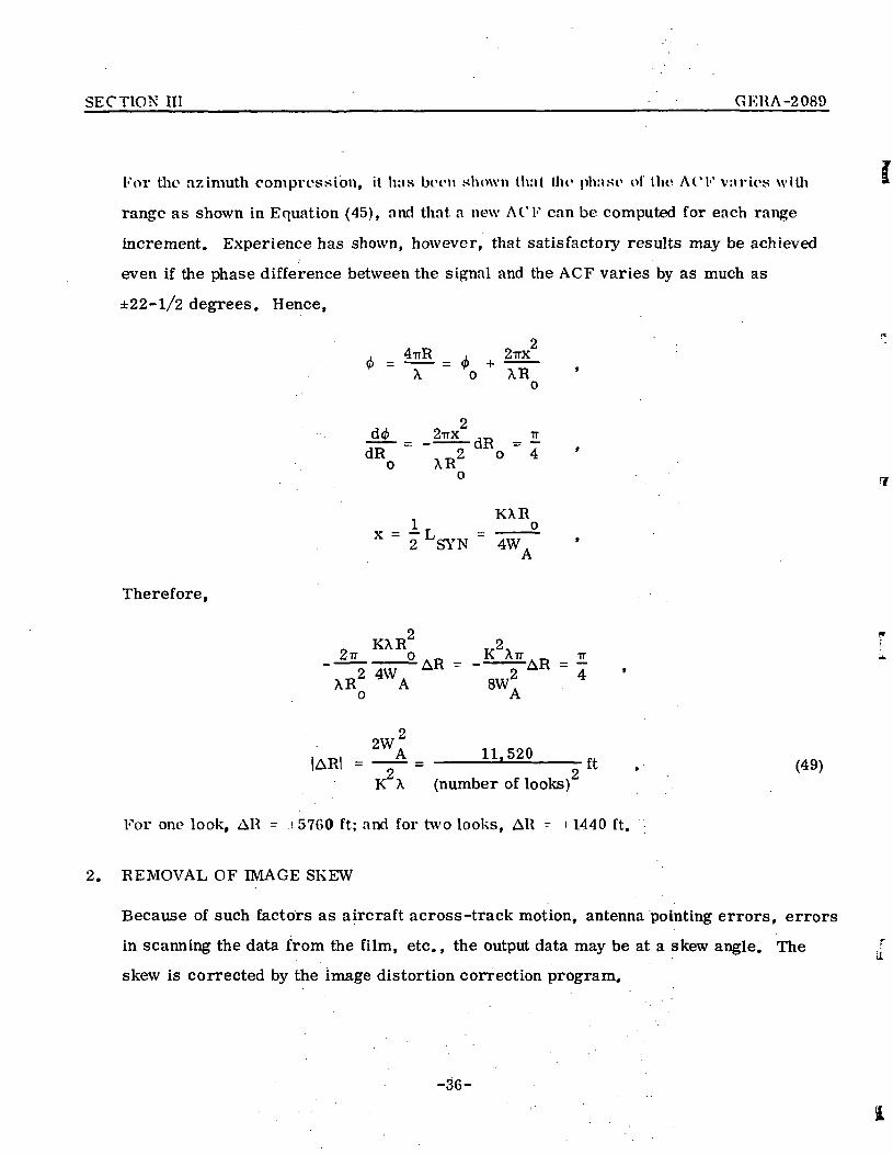
For the azimuth compression, it has been shown that the phase of the Al 'F varies with

range as shown in Equation (45), and that a new ACT can be computed for each range

increment. Experience has shown, however, that satisfactory results may be achieved

even if the phase difference between the signal and the ACF varies by as much as

±22-1/2 degrees. Hence,

2& _ 4'"R _ , 2TTX

X o + XRo

. 2d(j) _ 2-TTX _ TT

o XRo

KXRir _ o2 SYN 4WAA

Therefore,

2_ KXR »,2,

2 4W 2XR A 8WT

o A

2W

.-jA. "-520 , ft . ,49,K X (number of looks)

For one look, AR = :i 5760 ft; and for two looks, AU ^ i 1440 ft.

2. REMOVAL OF IMAGE SKEW

Because of such factors as aircraft across-track motion, antenna pointing errors, errors

in scanning the data from the film, etc., the output data may be at a skew angle. The

skew is corrected by the image distortion correction program.

-36-

SECTION III ___ _ '' _ GERA-2089

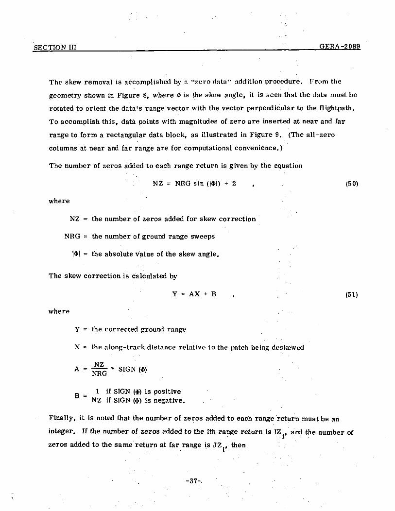
The skew removal is accomplished by a "zero data" addition procedure. From the

geometry shown in Figure 8, where 0 is the skew angle, it is seen that the data must be

rotated to orient the data's range vector with the vector perpendicular to the flightpath.

To accomplish this, data points with magnitudes of zero are inserted at near and far

range to form a rectangular data block, as illustrated in Figure 9. (The all -zero

columns at near and far range are for computational convenience.)

The number of zeros added to each range return is given by the equation

NZ = NRG sin (|$l) + 2 . (50)

where

NZ = the number of zeros added for skew correction

NRG = the number of ground range sweeps

|$! = the absolute value of the skew angle.

The skew correction is calculated by

Y - AX f B , (51)

where

Y = the corrected ground range

X = the along -track distance relative to the patch being deskewed

A = * SIGN <*>1 if SIGN ($) is positive

NZ if SIGN ($) is negative.

Finally, it is noted that the number of zeros added to each range return must be an

integer. If the number of zeros added to the ith range return is IZ., and the number of

zeros added to the same return at far range is JZ., then

-37-

SECTION in GERA-2089

4779-7

PERPENDICULAR-TO AIRCRAFTFLIGHTPATH

EFFECTIVE ANTENNAPOINTING ANGLE

AIRCRAFT FLIGHTPATH

Figure 8 - Geometry of Data Skew

GROUND RANGE SWATH BEFORE SKEW CORRECTION

00o ooo o o

o o o oo o oo

ooo ooY = 0

RANGE (Y)

4779-8

-(- IMPLIES VALID DATA POINT

IMPLIES ADDED ZERO DATA POINT

Figure 9 - Format of Data after Skew Correction

-38-

SECTION III : GEKA-2089

IZi = (< A ) < J ) ' "I HOUNDED (52)

JZ. = NZ - IZ. (53)

The placement of the zeros is illustrated in Figure 10.

3. SCALE FACTOR CORRECTION

Upon completion of the azimuth compression, the output data sample points may be

spaced differently in range and azimuth. The image will consequently appear distorted

because of the differing range and azimuth resolution. To compensate for this, a scale

factor correction may be necessary.

Scale factor correction is accomplished by linear interpolation on the azimuth data. For

example, assume that an azimuth sample was calculated every 12 feet, and that 30 feet

was desired between samples in both dimensions. Then, to achieve azimuth samples

spaced by 30 feet,

NRG

O O O + ++ + + + + +QOO

IZ

4779-9

Figure 10 - Placement of Zero Data Points

-39-


Yl = Yl

Y2 = I(Y3 + Y4>

Y3 = Y6 (54)

etc.

It is observed that data points Y and Y are not utilized in the foregoing calculation.2 5

Therefore, an increase in the processing rate is possible, because these points need

not be calculated.

-40-

GERA-2089

SECTION IV - CONCLUSIONS

The results of the geometric distortion analysis indicate that the distortions in AN/APQ-102A

imagery are primarily the result of navigation system errors that are external to the radar

system itself. These distortions can be rather high in magnitude (e.g_., one percent), but

have a low spatial frequency. As such, it is a relatively simple task to measure and remove

the geometric distortion. Measurement is accomplished by comparing image distances

(obtained from a map) between known ground features with good distances. Using this tech-

nique, the residual distortions were under 100 meters. Computer programs to measure and

correct these distortions were delivered as part of the contract effort.

The major program effort consisted of generating a computer program to digitally process

AN/APQ-102A phase history data. This program was checked out and validated at the

customer's facility—thus providing a capability of processing subsequent AN/APQ-102A

data without contractor support.

-41-

GERA-2089

APPENDIX A -

TARGET SIMULATOR

A-l

APPENDIX A GERA-2089

C PRQG.9-75 P6INT TARGET GFNERATflRC

DIKENSieN IDATA (8800)*MTR1(27)C

3 C N * • 2BIS- .316

1592^,535897

REMND 2C

200 CPNT-IMJEREAD 98PRINT 1C1PRINT 102PRINT 99/MTR1 .

C 9UTPUT RECORD 1 BN TAPEC

CALL TAPE RI (^TRDcCc CAZ DISTANCE PER AZIMUTH SAMPLEc DRG DISTANCE PF:R RANGE SAMPLEc Azers AZIMUTH! BFFSETcc HF ALTITUPE IN FECTc RP RANGE IM FEETC PHIO PHASE ANGLEC

REAP lOO'PAZ/DRG/AZ^FSPRINT 103/DAZ*DRG»AZ0FS

PRINT lO<»*HF,Ke/PHIB201 C8NTINUE

CC K RG ELEMENTC N AZ ELEMENT

ORIGINAL PAGE ISOF POOR QUALTHI

A-3

APPENDIX A • GERA-2089

c NRe NUMPFR er RANGESc

RFAC 105*M*N*N'RPIF(NRD) 198* 198* 199

198 CONTINUE"CALL EXIT

199 CONTINUEPRIM 106*M*N-*NRB

C RG LOOPC

?02 I^l l7

203 CONTINUE'c CALCULATE AZ INDEX LIMITSc

IC LIMIT INDICESC

PRINT 107/NAZ1/NAZ2c END OF I^PK KEEPING* DO THE CALCULATIONSc

AN««NAZ

fiB--2.*Pl«AZ8FSPRIM 109/AA/BUIY»CIF(\AZ1-8800)20P*?0C>*?09

C OUTPUT FIRST HALF 8F AZ SWEEP :

C .

- - ... •' - - '•' • " - . • . • II

ORIGINAL PAGE ISOF POOR QUALETYi

A-4. .- . '' . • • ' • • ' ' • ' ' t t .


209 CONTINUECALL TAPE^/2 ( IDATA, IX, I Y )IY-??COJAZ«\AZ1-8800

208 CONTINUEC AZ L08PC

DO 20A IAZ.VAZ1/NAZ2PHIe(AA»AN*PP )»AN+PHIP

C TAKF CSS,ADD BUS AND SCALEC

C CONVERT TPAivSMSSIQN T6 DENSITYC • •

C NOW SCALE T» « BITSC

IDATA(jAZ)«TD

G« T6 197PRIM 10»*AN,PHI«T*0»ID

197 CPNTIMJE

C

205C QUTPLT MALF 6F AZ SWEEPC

CALL TAPEW2(IDATA*IX»IY)DO 206 I-1/8800IDATA(I).0

206 C9NTINJF

JAZ-1C

2.0* C9NTIKUE210

A-5


C eilTFfT SECOND HALF 9F AZ SWEEPC

CALL TAPEW2(IDATA,IX/IY)IF( JY)2l2/2l2*2ll

212 CONTINUEIY«38CO

213 CPMa? T9 210

Ell C?MIMJ'::c

202 CPM1NUEC

GP T6 201

99 FeRyAT(6X8QAl )IOC FH^ÂT (8E10.<»)101 F*RKAT<6X1<HJPK8GRAM 9-75* 20X3QHG6PDYEAR AER0SPACE C8RP8RAT ION* / )102 F f ? R K A T ( 6 X 2 g H p e i M T A R G E T G E N E R A T 0 K / / )103 r O R ^ A T ( 6 X 5 H P A 2 -E12.5* 5X5MDRG «El2 t5 ,5X5HAZ9FS/El2»5/ / )lO'* F t ) fÂT(6x5HnF -F12 • 1* 5x5HRO -F12* l*5X5HPHl8»Fl2.3* / )105 Fe«ÂT(16I5)106 F8RÂT(6X-*3HK .I7/5X/3HN . I7/5X3HNRB* 17, / )107 Ff>RNAT(6X2lMA2lÛTH SAMPLE L I Ml TS/ 2 1 10>/ )108109

END

A-G


SUBROUTINE" T A P E F l ( M T R l )DIMENSION MTRl (27)

c THIS ROUTINE is FOR WRITING RECORD i w i s s MAG TAPEC F0RNAT (27 CHARACTERS)C 27 CHARACTERS OF WHICH PO OR 22 ARE NEEDED

"RITE TAPE 2* KTR1RETURNEND

NE TAPEW2(irATA*lX,IY)C THIS R9UTINE IS F^R OUTPUT TO MAGNETICC TAPr FflR THF SECOND AND SUBSEQUENT RECORDS

DIMENSION .IDATA(8800)WRITE TAPE ?/ IDATARETURN

100 FPRÂTfI6,1X,40I3)RETURN • • •END

A-7

G ERA-2 089

APPENDIX B -

AZIMUTH PROCESSING

B-l

APPENDIX B GERA-2089

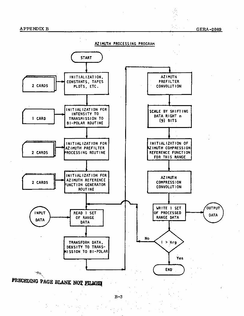
AZIMUTH PROCESSING PROGRAM

c START

2 CARDS

r

INITIALIZATION,CONSTANTS, TAPES

PLOTS, ETC.

1 CARD

INITIALIZATION FORINTENSITY TO

TRANSMISSION TOBI-POLAR ROUTINE

2 CARDS

INITIALIZATION FORAZIMUTH PREFILTER'ROCESSING ROUTINE

2 CARDS

INITIALIZATION FORAZIMUTH REFERENCE'UNCTION GENERATOR

ROUTINE

READ 1 SETOF RANGE

DATA

TRANSFORM DATA,DENSITY TO TRANS-

MISSION TO BI-POLAR

PAGE BLANK

AZIMUTHPREFILTER

CONVOLUTION

SCALE BY SHIFTINGDATA RIGHT n

(9) BITS

INITIALIZATION OFAZIMUTH COMPRESSIONREFERENCE FUNCTION

FOR THIS RANGE

AZIMUTHCOMPRESSIONCONVOLUTION

WRITE I SETOF PROCESSEDRANGE DATA

B-3


Card Input to the Azimuth Processing Program

Card I 80 column description card.

Card 2 N number of data points/record.(2 values) (Azimuth samples per range bin.)

NRG number of range bins to be processed.

Card 3 SCL « density represented by a value of 255-(3 values) TMEAN « mean transmission for bipolar calculations.

SCL2 - second scale to convert to integer.

These are for Initialization of the Density toTransmission to Bipolar Routine.

Typical Data: SCL = 2 or 3, TMEAN = .38, SCL2 = 6*» or 128.

Card 4(3 values)

Card 5(1 value)

NLOOK = number of looks, 1 or 2.K = K in COS[2PI K I/N], (see azimuth prefilter formula).

NB - number of bits in the quantized output.

PHIO phase offset in degrees. (This is an arbitrary input.)

Cards A and 5 are for the azimuth prefilter reference functiongenerator routine.

Card 6 DAZ = distance per azimuth sample in feet.(3 values) DRG = distance per range sample in feet.

AZOFS = azimuth offset frequency in cycles/ft on ground.

Card 7 HF = altitude in feet.(3 values) RO = range in feet.

PHIO *> phase angle in radians.

Cards 6 and 7 are for initialization of the compressionreference generator routine. :

If

B-4

APPENDIX B _______^_ GERA-2089

C PAIN LIME PROCESSING 8F IMAGERYC

ON MM(20)* RR ( 44 )

ON IfM17fOO)PN KD(931)ON ICR(930)* ICOO30)

EQUIVALENCE ( ID(1)*J0(44))ECUIVALENCE (KC(931)* ID(1 ) )N 3 1760CJT«1ITa2TAPE ?. IN* TAPE 1 OUT

200 CONTINUEREMIND ITREWIND jTNW • MO CPL OISCRIPTI6N

PRINT

READPRINT 102*N»NkGNT»N< = CCALL CNTRBP (ID*K)CALL REFGFN (IR/NPR)

\LtJ9K m 1

220 C9NT1KUENL09K • 2

221 CRNTINUE

CALL CMPREF ( I C R * I C Q * M )CC L99P 9NC

DRWINAJJDP POOR QUALTTY1

B-5


Cr? 201 KRG»1*NRGN » NTCALL T'APF.IN ( ID*NT)K • MCALL DNTRPP (ID/OCALL PSINTD (in,N)

•MP • \

CALL AZPRT ( ID/ TR*N,NPR,JD*NP)CC SHIFT DATA BY 9 BITSC

C»}. 207 I » 1* KPJD( ! ) « JH(I )/51P

207 CRNTIMJECALL PRINTD (JD*Np)CALL PLOTD(JD/NP)

CALL\;^ « rCALL PRINTD ( ICR/y)CALL FRIMD (icc/^)

CNS « 9CALL AZC8MP ( JD, ICR»ICO*NP*NR*NS^KD)\ » NP/NSGP Tft (2P^/?P?), NLP8K

222 CCNTIN-JE:CC TK3 LP3K CALCULATI8NSC

\P > N-3D6 223 I • 1* NPKC(D

223 CeNIN • \P

22* C6NTIMJE

\1

DEKHNAIi PAGE ISDC POOR QUALITY

B-6

APPENDIX B • GERA-2089

CALL PRTMO (KD/N)

IF(fAX-KD( I ) )?05* 506/206205 CBNTINUE

PRIM 10^'NRG* I,ce\TiN\p»\+i0^ ?03

203 CP.NITCA(_L

201 CONTINUECALL PLOTD (KC/N)Gfi TO 2oCCALL PL6TC (io*o^KITE TAFF JT, ( J0'< I)* I •!*< J

93 FR^KAT (6X20A4//)99 F9R?"AT (20A^»)100 FfiRyAT (8F10»4)101 F&RfAT (36X35HIÂGE PR8CESSING G.A.Ci PR8G 9-7S///)102 F*R"AT(6Xi9MNUMBER 9F SAMPLES •* I 7t 5X22HNUMBER 6F RANGE BjNS »I7

I*/)101* FPRKAT (110*3X1019)

END

OF POOR

B-7

APPENDIX JB : '• . G ERA-2 089

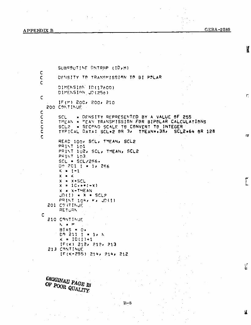
SU9R9UTINF DMTRpP (ID/M)Cc DENSITY TP TRANSMISSION TP BI P?LARC

0N' ID(l7fCO)f>N JD(256)

c ••JF(M) 20C* 200* 210

200 C9MIKUF.Cc SCL » DFMSITY REPRESENTED BY A VALUE er 255C TMÂN « MCAV TRAN3NISSI6N FSR BIPOLAR CALCULATIONSC SCL? « SFCPNO SCALF TO CONVERT T0 INTEGERC TYPICAL DATA! SCL»2 9R 3t TMEAN««38' SCL2"6<» 6R 128C «

READ ioo/ SCL» TVIEAN/ scL2PRINT lol-PRIM 102* SCL* TMEAN, SCL2PHJKT 103. •SCL • SCL/256.D* ?C1 I • 1* ?F6< « 1-1x . <X » x«SCL ' . jX * 1C»»«( -X) U

X « X-TMEANJD( I ) • X * SCL?PRINT 10** *' JPU)

201 CS'JT

C210

\ a M

BIAS « OfDP 211 I • 1*< » IC( I )+lIF(K) 212* ?!

213 CPN'TIMIEIF«-255) 211** ?!** 212

if

B-8


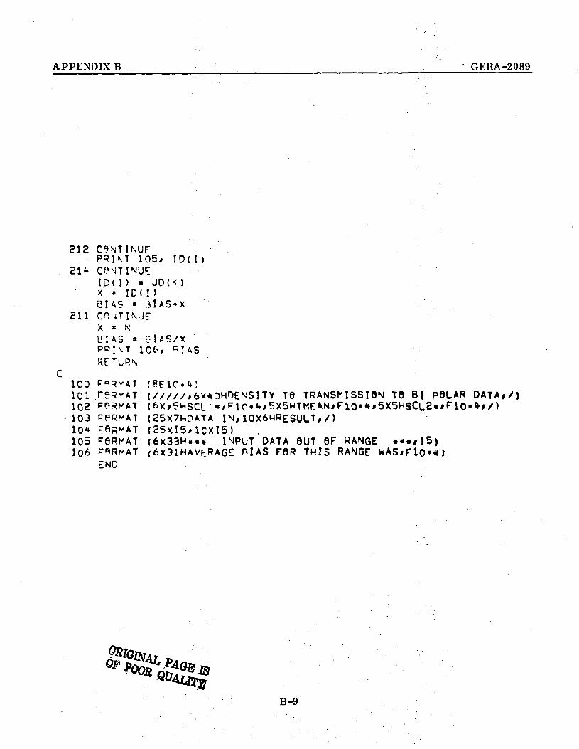
212 CONTINUEP R I M 105, 1 0 ( 1 )

I D ( I ) « J D ( K )X » ID(DB I A S » U l A S * X

211 CONTINUEX » N1

CIAS « eus/yPRINT 106, BjAgRFTLRN

C

101 FSRÂT (/////,6X40HOENSITY T8 TRANSMISSION T8 Bl POLAR DATA,/)102 FPRÂT (6X/5MSCL •*Floi<»/5X5HTHEAN*FlO»<»*5X5HSCL2«»l '• "103 FPRyAT (25X7HDATA IN,10X6MRESULT*/)10* F6R"AT (25X15*1CXI5)105 FBRIÂT (6X33H««« INPUT DATA 8UT 8F RANGE **«*I5)106 F^Rh'AT (6X31HAVF.RAGE RlAS F8R THIS RANGE WAS/FlO'f)

END

B-9

APPENDIX B ' GERA-2089

SUBROUTINE ÊFGrN ( IR,N)C A Z I M U T H PREHLTtR RFFp.RFNCE FUNCTION GENERATORc TWO DATA CARDSc

DIMENSION IRU4)

CCC \LRPK. • M.'K=>EK *? LPOKSC < • .* IN CeS(2PJ K I/N)c \r B NU^FEK PF BITS IN THE QUANTIZEDcC PHIf? » .PHASE

PI - 3M'»l5Q26535897Ê AC 103* NLBPK/ Kf NBOR JNT 10** MppK/ K/ NB

P R I N T - ' l Q S * PHI9SC « (2

G6 T6 ( 2 0 1 * 2 0 2 ) * NLR8K201 CPf iTINUF

\ B i*420? CONTINur

xt, • \PRINT lCfXÎN a C»

XNAX a \ -1A = *CtNB » 6

X » C-CALL TAyLPR ( X^ I N, XÎAX* A*N8* X* V<TN, 0 )DP 203 .1 • 1* \ 'A • (!•!)*<A a 2 « * P l « A / X M + P H i eX • 1-1CALL TAYLOR ( X M I N * X M A X * A * N B * X * W T N / D

B-10


203 CONTINUECC PUT APP|_ITUCE WFIGHT1NG HEREC

I « 1» N

IF(P.R(I-J ) 205, ?05, 206£05 CONTINUE

206

P R I M 107*1, I KC P N T I \ U F .

100103 FSRÂT (1615)10* WAT (6X7HNLBPK -*I3*5X3HK «*!3*5X*mNB «*I3*/)105 F9RVAT (6X7HPMJ? »,F10»*,/)106107 FflRÂT (-15X2-I 11 >

END .

B-ll

APPENDIX B CERA-2089

(ID* IR,M,NPR,A7IVUTH PREÎLTFR WALLBPS DATA

IPU<*)/ JOU5)10(17600)

? >- —IS«C08 ?C3 j«lX « I+j-1IS«TD«)»IR( J)*JS

£03 CONTINUEJD( I )*1S

208 CPNTIMJPRETURNEND

B-12

APPENDIX B _ GERA-2089

SU3R6i:TlMF C^PRFF ( I R / I Q / MC?fPRKSSlPN REFrRrNCF GENERATOR

CC f > -1 f)R .? FPP INITIALIZATI8N ABS(N) • NL60KSCc f RETURNED AS KU^BFTR OF POINTS IN THEc

I F ( N ) 2oc» ?lc* 210200 CONTINUE

PI - 3»lM5926535S t '7» .10??30.

TWF -1.4?XK «

C :CC DAZ « DISTANCE PE" AZIMUTH SAMPLEC OPO • DISTA\'CF PE* RANGE SAMPLEC AZOPS • AZIMUTH OFFSETCc *r « ALTTTUDT IN FEETc .Re • RANGE IN FEETc PMJO « PHASE; ANGLEccC \DBC = D5 DPVA FOR TAYLPR WEIGHTING ( 4Q )C NBAS • \BAR F9R TAYL0R WEIGHTING (6)C \PITS • NbMREK ffP BITS IN REF FUNCTIONS 6*7/8C

• READ 100* DAZ* CRG* AZ8FSPRINT 103* OAZ* DRQ» AZ6FSREAD 100' HF, R8, PHJ0PPINT 1Q4* HF* R0» PHI8ND3C • 40NPAP « 6 '

ORIGINAL PAGE ISOF POOR QUAUTX?

B-13

APPENDIX B CERA-2089

NPITS - PpejS'T 105* NC3D* NBAR* N'BITSDPI) «SC «PN « •5»XK«ALAK/(WA»DAZ)FN a PN»XLQPK

201 CONTINUE.

2ic

NAZ • RS«PN/2.+.5-NAZ

N •

V « N

XÎ\ a -NAZXMAX = K'AZAA « .S'^PABB « -P.«PI»A79FSPPJM 106* AA* PBCALL TAvLCR (XNlN,x-lAX*DBD/NBAR*AN1, AMP/0) rrn ?ii i . i* \ \CALLPHI « ( AA»Ak.*BB)»AN-t-PHI9A\

I f ( I ) • RI r. ( i ) « c

100 FPRr-'AT (8T10.H)101102103 FBRfAT (6X5MDAZ .*E12.5»5x5MORG »*E12 t5* 5X5HAZ8FS*El2»5/10* FPFÂT (tX5HHF .*Fl2» 1*5X5HR8 »*F 12» 1» 5X5HP.Hlfl«»Fl2»3*105 FgRr'AT (6X6HNDBP «* 15, 5X6HNBAR •, I5,5X6HNBITS«> 15, / )106

B-14

APPENDIX B : GERA-2089

( ID/ IR*IQ*N,NR/NS*JD)AZIMUTH CPMPRESSI*N FILTER

in(i7600)JP(<*5)IR(93C>* IG<930>

C \ • \UMBFR 9F P9INTS IN THE DATAc \R « \U^PER OF -POINTS IN THE REFERENCEc \s • NUMBER eF POINTS FRBM OUTPUT SAMPLE TO NEXT OUTPUT SAMPLEcc ID is DATAC wO IS OUTPUTc IR is REAL REF CHANNELc ic is GUAD REF CHANNELc

N » N-NRK * 121 20C I • 1* ' K* MSISR • 0ISC • 05? 201 J - \t KPL » J*I-1wR « IH(J)«ID(L)/256JC « I2U) •IC(L)/256ISRISQ

201<K<K «15$ «ISR «IS « ISRJD«)-IS

.200RETURN

B-15


SUBS5LTINF TAYLPR ( X" I Nj» XPAX/ A*\B, X/ AN|S, JeB )C . THIS SUnRRUTINE CALCULATES THE TAYLSR APERTUREC XK IN X MAX-XÎ\ r RAN'GF QF APERTURE!C XMAX [-C A s DB DPWN f»F FIRST SIDEL3BE IN TAYL8R ANTENNA PATTERNC NP = N-PAR (TAYLOR'S CONSTANT)C X • VALUFf AT WHICH ONE POINT 6F APERTURE IS WANTEDC ANS • THE ÊTb»NEO ANSWERC JOB « 0 TÎS IS A NEW XMlN*XMAX*A AND NB DATA SETc « i USE PREVIOUS XMIN;XMAX«A AND NB DATA CALCULATIONS

DlMFNSIpN F(20* C(10)* FF(2) „.EQUIVALENCE (FF(2),F(1))

C . • . .iF( t a«e> 11* 11* 12

11 CPNT1NJFD a Xf"AX-X*INPI « s-iîSâesasBg?TPI • 2.«FIP ( 0 ) 5 1 .

. o? ic i = i/ ?o rAR-G - I LF( I ) = F( I-1)*ARG

10 CONTINUEAA » 10.««(ABS(A)/20«)CALL A«C6SH (AA,ETA)AA « ETA/PIA? • AA*AAENB « NBNf3M » NP-1S I G » E 'DH 20 NF.NJ • N

S « !•Dfl 30 M • 1

ZM . SIG*SQPT'(A24>(EM».5)*«2)S • S«(i»-EN'?/(ZM»ZM) )

B-1G

APPENDIX B •" G ERA-2 089

30 CONTINUEC(N) = S

20 CONTINUE12

F

ANS-40 C'.vN

cPRIM ICC* A, A'P .PRINT 1C3* AA» SIGPRIM 101* ̂ * C(N)PKIM 102

IOC FPRÂT |5X17HSL'RR*UTINE TAYL9R/ //5X17HFJRST SIDEL8BE « /F6.J*1 3H DE,lcX8*N'-BAR • / I 2, //1QX12HC8EFF ICIENTS )

102 FflRNAT (1H1)'103 F^RÂT (18X?HAA*17X3HSIG*/2(5xEl5.8)*/)

END

ORIGINAL PAGE 13OF POOR QUALOT

B-17


MF. ARCPSHc

UP = u«uJF(L2-i.) 11, 11,

12 CONTINUEA «

11 CONTINUEA . 0»PRINT 101HETLRN

101 TPRiÂT (1HO/5X56M*.* TAKIMG ARCPSH BF A NUMBER LESS THAN 1 JMP0SSIiSLt «*«>/) r

B-18

GERA-2089

APPENDIX C -

DISTORTION ANALYSIS

\

C-l

Page intentionally left blank

APPENDIX C GERA-2089

19135 »PR 03»'751. OOJBLE PRECISION Ex I 512>»EY(512>2« OI-ENSIOs IBUFUJOO)3. DOjBLE PRECISION xI 512)/YI 512)if I512)*«lS12»*A/BjC'EI512>*D/F,0*X1»• 1(512)**'AL'Al'A2'A3<»*' V»V1<A3I20>'XEI512)<YE(512)'C1'Yl<5« 2512)6. DI-EsSION AAt16)'AAi(20)*AA2(20)*AA3(20l*AA»(20l*NE(20)*C»(20>*CBt7. 12018. DliE'.SICN ALPHA<2'512>9. CO-ÔN s^P-IS'i-lN/SCPLT/SCEROR

10. C X 4S-; r ARE THfc TRAC< AND RANGE COORDINATES ON THE IMA3ERV'11. C ">EspECTIvEtY. ^ ANO S ARE THE "AP POINTS AND SHOULD BE WITHIN 4512« C CE3"FES OF Ti*E 1'iAQERY POlNTS»Nl AND N2 SHOULD LIE13. C is T-E T(?AC« DIRECTION w]TM Nl TO TM£ LEFT OF N2«l»« CALL PLOTSIiByf*ioco»7)15. C PLOT T»PE ON 18316. R E A D ! 1 < 5 5 > A A 1 « * A 2 < A A 3 / A A 417. 55 F O R ~ A T ( 2 0 A « > )18. 25 R E A D ) 1/1 ) N / M < « 2 / A A19. 1 F C R * A T ( 3 I 5 4 l 6 A » >20> IF |N )20<20 '3021. 30 CONTINUE22* C SCALE OP PLOT ASO S C A L E OF ERRORS2 3 * R E A D ( l » 3 > S C P L T j S C E R 3 92*. DO 2 I - 1 < N2 5 * R E A O I 1 , 2 1 1 I P ( I » * 3 I I )26. 211 F 0 9 r A T ( 3 F 1 0 « 2 )2 7 . 2 R E A D ! 1 * 3 4 5 1 X 1 I > < Y C30. C CHAS3E FOR1AT CAR331. • 3 P09MAT(grio.3)32> 3*5 F O * - A T ( 2 F 1 0 « 3 « A » » A » )33. C 9 0 T A T I O N OF 1A" SECTION3*» A a O A T A N ( ( Y ( N 2 ) » Y ( S l ) ) / I X ( N 2 ) * X ( N l ) l )3S> B - O A T A - , 1 IC IN21-3 IM ) I / IP ( N2 I-PIN1) ) I36* A - » » 937. 1003 A-.3i.«-A38. A :£0-57 .29578»A39. 00 * I - l / N*»0> B « o i l )•»!• »( I )•»( I ) » O C O S C A l » 3 ( I I»DSIN(-A)^2> « ;( I 1 - 0 1 I I ' l O C O S I - A ) ) - B » ( O S l N ( . A ) )*3 ' CALL L S F I \ , n , Y « x « 3 / p < A / B I•>•>• 00 5 I«ljN»5. 5 El I ) - A » Y ( I l»B-;(I I•»6. CAUL LSFI 1,N,P,Y,E,3»A,B I* ' • A " D A T A N ( A »*8« ADEO-AOE3»57.29578»A»9« H R I T E < 3 « 8 0 0 I A O E O50> BOO FORHATdx* ' ANQJLAR R O T A T I O N • '*FlO«»* * DEOREES'I51« 00 6 I- 1/N . . .5 2 * B » » ( I )53> PI I ) « P ( I I » ( D C O S I - A I 1 * 0 ( I I • (08INI-A)I

,,

APPENDING . . . C.ERA-2089

I

19.'35 APR 03* '795«». 6 St 1 )«3t 1 )*DCOSl-*>-a»OSlNl-A)55- C PLOT SCALING SECTION56- P*157. 2-58* DO59« JFI60« 800 IF<6l« CALL PLOT<0.,1««-3I

63> *!•»6*' 1005 BY«365* AL"B66* C A L L L S F ( ' l « N « X * V « P « 3 « « « B )67. c TE-PO«A<»Y SECTION TO MEASURE iiA3E«r DISTORTION AFTER CORRECT ALIONMENT6B> *8«(*l»»)/2.69« 00 51 1»1»N70" xl ( I )«A2»X| I I7l« 51 »1 I I )-»2»YI II7?. *3«0.73 • *»«0 .7»« S3 5? t"l<N76* *3-*3»Xl I I )«PI I )76" 52 «»«A»»Yl( I 1-21 I )77« »3«A3/S78* »».»»/-,79« DC 53 I-1'N£0* xl ( I > » x i CALL EPLQT (p,a/XE»YE,Ex,EY/AAi/AA)87. G3 TO 5*as* 57 CONTI^JE89« 00 70 I»1»N90- Xl I I )-»»x I I )91 • 70 Yl ( I )»*1»Y( I )92* »3-0.93« A»«0«9«.« 00 70S I«1»S95« A3.»3«xl(I I-PI I )96« 705 A*«A*»Y1 ( I !-;-A*102" CALL103* «R!TE<3/56)AA210*« CALL EPLQT(P,Q4KE/ Y£iEKjEY*AA2/ AAI105" 00 TO 5*106« 67 CONTINUE

c-4


107-108«109-110*111-112*113.ii*«115.lib*117.118*US'i2C«121-122«123«

125*126>127.128*

13C-131>132«133*13»«135*136»137.138*13»>

1*1-

!*>*«

1*7.

150>151*152>153.15*.155.156.187.158.159«

19:35 APR 03* *79C-.CC05D-D.CO 7 1-1>*E « A » X DA3SlEl I ) I

a xii i i « x i i > » A L » Y I nC«LL LSM 1«N«X1»Y»P,3,A*8ICO 9 J-l*s

9 F«r«CA3S( A»xl39*Rr SECTION

CO 71 IVI I 1 )««2»Y| I )Xi( I )-*2»xi I )xi 1 1 »-xi 1 1 )»*L»nti )QO 72 I-1«N43«*3»m ( 1 |.P( J )»»«4»»tl ( I 1-01 I >A3-»3/s

CO 73 I « l « \xil I ) - x l ( I )-*3YKI 1 - Y 1 I I )•*»C*LLCALL E?LOT(P«Q<XE*YE«EX/EYJAA3«AA>GO TO 5*CONTIS-jE00 74 I-l/NXI I I )-x( I l»AL»r< I )XI I I )«*»Xl( I )Yl ( [ l«*l»Y( I )A3-0.A*«0«

ORIGINAL PAGE BQUAUT3J.

C-5

APPENDIX C . GERA-2089

19!35 APR 03* '7516C« CO 713 I-l/N161 • A3"*3*xl ( I I-PI I )163. 713 4*-A»»Yi ( I l.gt I I163. *

165. 00 71*166. X I I I )»Xl I I )-*3167. 71* VI ( I )-Yl ( I I. A*168. C»LL «16Sr« »RIT17:. CALL E°LOTIP,2<XE*YE*EX*EY*AA*,AA)171. 30 TO 5*172. 69 CC%Tl\jE173. *L-*L»l-57.?96l „17*. C SCALE CARDS -»0

176. »«ITEI3«15I A*A1« AL177. 15 rC^-*T(iox/>THE TR*C< DIRECTION SCALE FACTOR IB l!'*^!?***1 > THE178. iRAvSE DIRECTION'/XIOX/'SCAUE FACTOR 18 i:»<F12i*,». THE SHEAR 18 '179. 2*F6.g,' DEGREES1///!16C« 35 FO*-»T( 10X< 16A*I1B1« 30 TC 25182. 20 CONTINUE163t C ST4SOARD "RITE SECTION18*. 3C TC 75185« 5* *<•«<»! p-166. «RITE(3,58) [187. 58 FOR-ATtesx, 'TASuE I • RESIDUAL ERRORS ' //17X» ' POINT NUMBER '* 10X« • TR18b« 1*C< ERPO«'»1CX< 'RAN3E ERROR'//!189*19C« 60

192« SJ"Y«0.193. CO 21 J-1<N19*. S'J-"SJ"*XE( I )»x£( I )195" 21 SUMY-Sj-Y»YEt I )»YE( I )196* SU*Y"SU1Y/N .197. SU--SU1/N198«199.200"201> 22 FOR"AT(5X> 'X VARIANCE • '/FlO«**'Y VARIANCE202. 00 TO(37,67/6B>69*75I»KK2C3« 75 CONTINUE20*. CALL PLOTI 12«0<0.<999)205« CALL EXIT206* END

U

06


19:35 APR 03* '75

XII I3. C T-IS SECTION DOES A LEAST SQUARES FIT OF rl POINTS* STARTJNQ FROM»• C TH£ jTn POINT IS X AsD P6« <"j»"-lfe« A»0»7. 5-C.B> R-C<»• e-o.

ic« T-O.O .11. L-0«013' DO 1 I13> S-S»XII)

15« T-T»X( I »'•«! I )16> 1 U-U*X(

19« RETURN20. END

C-7


2«3t«•5«6*7.8«9«

15«16«17*

23*

CCjBtE

19! 35 AP* 03* *7SI*1/ 3 » X £ , Y E , E X » E r , A A A * A A l

PI 1 > »ul i l » X E t l > « Y E l l l j E x f

A A A / 9 0 « < 8 0 )

C*LL ei.OTI 3.5* J - i -31DC 1 I-1,N

( PI I l-Pllv. I /SC B LT

l X P 4 3 E /I /SCERORI X f A X » X P A O E

Y P A Q E - r P A O E - Y E l I I/SCE'JORC*LL

CALL S Y M 9 0 L l 8 « 0 0 0 * l « * <X«»AOE-XPAQE»12.C*LL P L O T ( X P A a E « 0 « / - 3 lRETURNE N D

.-

ff

I

19535 APS 03»'75J «S>3«*•5«b>7t8.9>

io»i i «12*13>!*•15»16.

xj I l )> tl I J l > " l 1 )/OI 1 )/A3( 1 )/ VEI 1 )/ V/Vl/XEl :C T*IS S.S«»CjTlNE CC T»E RAÂ^ ANp 'AP

CC 3 I-l/2i3 »3•:•

00 » I»1»NXEI I l - x l l I I-PI I I

* VE( I )"Yl I I )-0( I Ico s r-i/N*3t i )«*ai i I*DABSI XEI i ) )

5 A3(a>"AQ(2>*DABS( U( I ) IA0(l I»AO(1 I/SAQI2 )*AQ(2)/NRETURNEND

TM£ MIBTOORAM Or THE LENQTM OI^FERENCES BETWEENPOINTS/ A6 WELL AS THE ABSOLUTE ERRORS AND CEPICD

C-8

CERA-2 08 9

APPENDIX D -

IMAGE DISTORTION CORRECTION

D-l

APPENDIX D GERA-2089

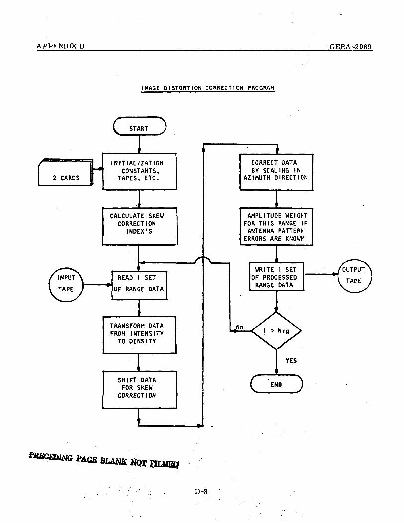
IMAGE DISTORTION CORRECTION PROGRAM

1 2 CARDS

^ START J

"

INITIALIZATIONCONSTANTS,

TAPES, ETC.

1CALCULATE SKEW

CORRECTIONINDEX'S

1 '

READ SET

OF RANGE DATA

, ,

TRANSFORM DATAFROM INTENSITY

TO DENSITY

1SHIFT DATA

FOR SKEWCORRECTION

1

/*

*CORRECT DATABY SCALING IN

AZIMUTH DIRECTION

1AMPLITUDE WEIGHT

FOR THIS RANGE IFANTENNA PATTERN

ERRORS ARE KNOWN

1 _WRITE 1 SET /OUTPUT

OF PROCESSED *t T.pf.DAurr r\ATA \ '"rtiKANuC UHIM \

J -W12-XT> NrgN

1 YES

C END )

D-3


Card Input to the Image Distortion Correction program.

Card 1 ITN = Tape unit input-(4 values) ITO = Tape unit output.

NAZ = Number of azimuth samples per record,NRG «= Number of range elements.

Card 2 SAZ = Azimuth scale.SRG = Range scale.

SKEW = Skew or shear angle in degrees.(3 values) SRG = Range scale. T

D-4

• a


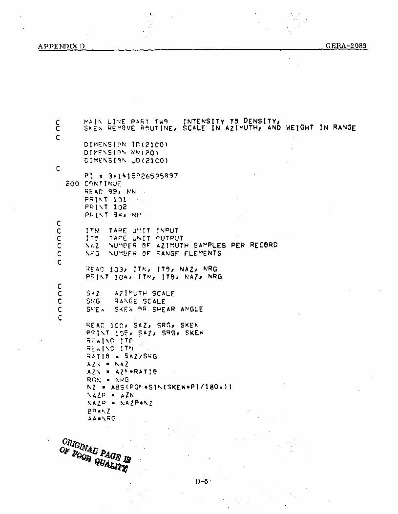
C M A I N LI\E P A R T Tw^ INTENSITY T8 DENSITY/c s*E'A REV9VE RPUTINE* SCALE IN AZIMUTH/ AND WEIGHT IN RANGE

DIMENSION IH{?1CO)

DIMENSION JD(21CO)C

PI « 3«1M5926535S97cOO CfiN'TlN'UF;

RF. ̂ 99, N'NPRINT 101PRINT 102

CC ITN TAPE U"IT INPUTC IT? TAPE UNIT PUTPUTC NAZ \UMPER RP" AZIMUTH SAMPLES PER RECORD

CSEAS io3/ ITN/ IT9, NAZ /PRINT 10** ITV/ IT9/ K 'AZ/

CC SAZ A Z I M U T H SCALEC SRG RANGE SCALEC SL:E^ S<E'/v ?R SÊAR A^ IGLEC

R E A H 100* s*z* SRG/ SKEWPRINT io5, S A Z * SRG, SKEWR F w I N D ITPR L X I N C I T NR . A T I 6 • S A Z / S K G

RG\ » NP.GNZ - A B S ( F G ^ • S I N ( 3 K E W « P I / 1 8 0 .NAZP • AZKN'AZP » N'AZP + NZBP-NZA A - N R G


IF (3KEW)c20»22C/2?l220 C?MI\'Ju

E5«l«A A a - A A

221 CONTINUECALL INTDFN (ID/-1)NZ = NZ + 2eÊ 6N FACH sior ALWAYSDP 2C1 IRG • 1* NRGKEAC TAPE ITN, (ID(K),K-ljNAZ)CALL INTDEM ID/N'AZ)

IZ » ÂX( IZ/1)JZ«NZ-IZK«l

D? T22 I !•!» IZJD(<) =0.<«<•»!

222 CONTINUECH 223 1 I » 1 * N A ZwD«) «IP( 1 1 )•< = K. 4 1

223 CONTINUED^ 224 n»l'JZJ^K) »0

224K « N «, Z + N ZCALL FII'H JP» i D j N » R A T i e )CALL RGir.GT (ID* IRQ, N)XSITE TAPr IT9, (ID(K)*K«1*N)N » ÎN( 130/N)PRIM 106* ( IO{<)»K«1»N)

201 CPNTINUEEND FILE IT?

PRINT 134

"

D-G

A PPE NDIX D GERA-2089

G" TQ 30C . '98 F°R"AT (6X2CA4//)99 rnÂT (?CAi»)100 F«ÂT (9F10.4)101 FPRÂT{6Xl4MPK-0r.RAM 9-75* 2QX30HG88DYEAR AER0SPACE C0RP9RATIGN* / )10? F^K.-AT <6X33HSKf:W GPRRECTJ8N AND SCALE PR6GRAH//)103 FiRi"AT(lM5)10* FC-RÂT{6X10Hl\PL-T TAPE/ I5*/6XllH8UTPUT TAPE/U//

1 MPSHNl^pE" BF AZIMUTH SAMPLES IS* 15* /6Xa7HNUMeER er "ANQE CLEMENHT5 IS/16//)

105 FPRÂT(6X8HAZ SCALE/F 12. 1 / 5X8HRG SCALE F13« 1/5X10MSKEW ANGLE F12.5

106 F ^ R v A T (1X/13CI1)FPKNAT (1H1)END

D-7

AI'I'KNIIIX I) P. Kit A-2 OK!)

SUBROUTINE FILL (ID,JD,N,R)CC in is THE INPUT ARRAYC JD IS THE 9UTPUT ARRAYC N IS THE NU^PED ?F POINTS IN THE INPUT ARRAYc R is THE INCKEÊMT RATIB

c N WILL BE RETURNED AS THE NUMBER PF OUTPUT PBcc

DIMENSION- jntsioo)c

i • iX * 1.X\> = N

O * ?. (T

cOOIF(x-XN) .-201*

201 CH'-JTIKUFXj = jIF(Y-xj) 203* 2c3/

£0<t CONTINUEJ a J* 1

•3'» T'3 201203 CPNT

Y « IC(J)Y . Y-DY»(XJ-X)IF(Y) 2o5/ 205/ 206

205 CPNT

GP T8 207206 CeNT

207 CONTINUEX » X*RI - 1*1G« T9 230

202 CONTINUEN » 1-1RETURNEND


c INTFNSITY IPc

fiN ID(?ico>

CC IF SCALF IS Nnj KN6WN USE M.-N F9K FIRST CALL

IF(V) 2cC/ ?10* 210200 CONTINjr

K * APS(^)K * IC{ 1 )Di ?01 I » ?» N' •K * MX(K* IH ( I ) )

201 Cf»MTI\UECC <IS - IMtNFITY SCAL9R USE 0 IF THE SCALE IS N9T KN0WNc <r$ - DENSITY SCALBR USE 128 FBR 0-2c

«?FAC 103* <IS/ fc-OSI F < K I S ) P02/ ?Q?/ 303

202C

E03PPJNT 102*ALC^ • 1 »/ALPG{255. )xs » KDS2!> ?C<» I » \f 256X * ID * ALGF«ALPG(X)

C )KDJ /I /301 TNlRP«0( I) - 8

cO<* CONTINUE

c210

De 211 \ m \,< t ID( I )/KTS

IDU ) *211 C6NTINUF.

10? FORMAT (6V5MKIS "•* IR* 10X5MKDS «/I10//)103 Fp

D-9

AIM'KNDIX I) fiKKA-208!)

(!D,M,N)CC 'ÂN^t; WEIGHTING F3R VrRTlCAL ANTENNA PATTED C6RRF.CTI8NC !* » RANGE" BIKc NEC ^ FMR I N I T I A L I Z A T I O N IF REQUIREDc

c i M t - \ s i r . \ i n c a i c o )c

I T i f ) 2 0 C > ?01* 2 0 1SOU

201 C?MINUF nr

I • It NCC PUT AEIP .HTIVG HrRFc

202 CONTINUERETURNEND

ORIGMAU PAGE ISOF POOR QUALITY

D-10

Documents

STUDY OF SYNTHETIC APERTURE RADAR (SAR) … · (SAP.) I8?,GSfy CHA-.ACTEFISTICS ... theoretical analysis consists of enumerating the known sources contributing to geometric ... steady-state