Embed Size (px)
Citation preview

Republic of Iraq Ministry of Higher Education and Scientific Research Al-Nahrain University College of Science
Study of Stopping Power and Range for Protons
A Thesis Submitted to the College of Science of Al-Nahrain University as
a Partial Fulfillment of the Requirements for the Degree of Master of Science in Physics
By Mustafa Abdul-Muhsen Abdul-Aali
(B.Sc., 2005)
1430 A.H. 2009 A.D.
Shawal October
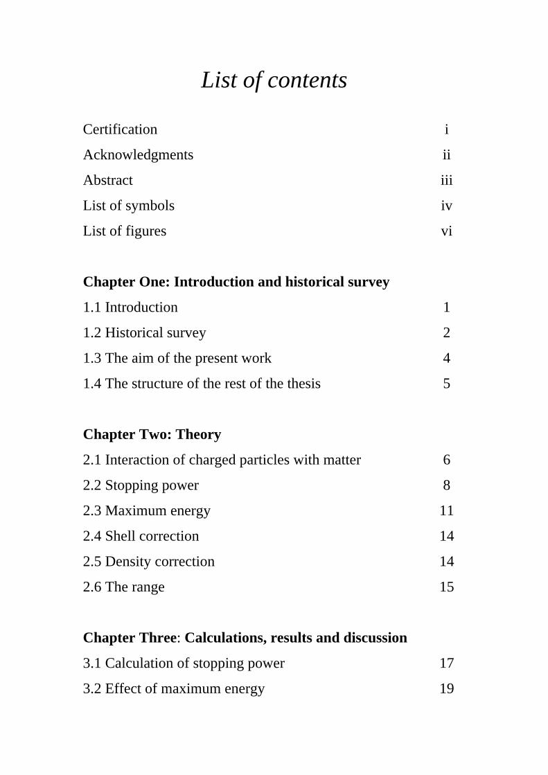
List of contents Certification i
Acknowledgments ii
Abstract iii
List of symbols iv
List of figures vi
Chapter One: Introduction and historical survey
1.1 Introduction 1
1.2 Historical survey 2
1.3 The aim of the present work 4
1.4 The structure of the rest of the thesis 5
Chapter Two: Theory
2.1 Interaction of charged particles with matter 6
2.2 Stopping power 8
2.3 Maximum energy 11
2.4 Shell correction 14
2.5 Density correction 14
2.6 The range 15
Chapter Three: Calculations, results and discussion
3.1 Calculation of stopping power 17
3.2 Effect of maximum energy 19
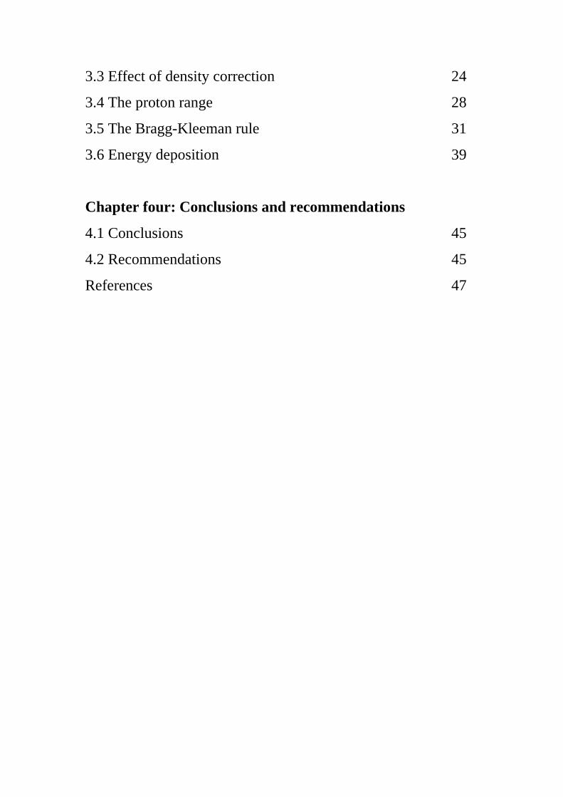
3.3 Effect of density correction 24
3.4 The proton range 28
3.5 The Bragg-Kleeman rule 31
3.6 Energy deposition 39
Chapter four: Conclusions and recommendations
4.1 Conclusions 45
4.2 Recommendations 45
References 47


ii
I would like to express my thanks and deep appreciation to my
supervisor, Dr. Mohammed A. Salih, for suggesting the project of
research, and for helpful comments and stimulating discussions
throughout the work.
I also like to express my thanks to the Dean of the College of Science
and to the Head of the Physics Department at Al- Nahrain Universty for
the facilities offered to me during this work.
My thanks are also due to my colleagues and friends at Al- Nahrain
Universty for their kind assistance.
Finlly, I am very grateful to my family for their patience and
encouragement throughout this work.
iii
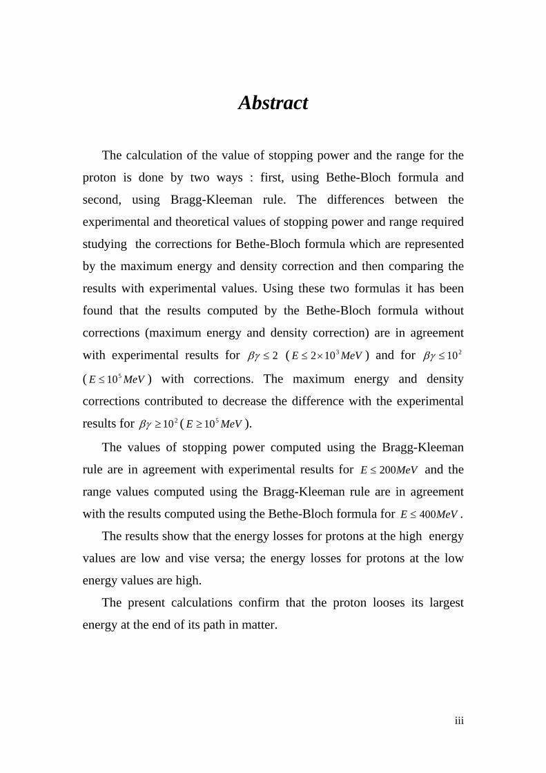
Abstract
The calculation of the value of stopping power and the range for the
proton is done by two ways : first, using Bethe-Bloch formula and
second, using Bragg-Kleeman rule. The differences between the
experimental and theoretical values of stopping power and range required
studying the corrections for Bethe-Bloch formula which are represented
by the maximum energy and density correction and then comparing the
results with experimental values. Using these two formulas it has been
found that the results computed by the Bethe-Bloch formula without
corrections (maximum energy and density correction) are in agreement
with experimental results for 2≤βγ ( MeVE 3102×≤ ) and for 210≤βγ
( MeVE 510≤ ) with corrections. The maximum energy and density
corrections contributed to decrease the difference with the experimental
results for 210≥βγ ( MeVE 510≥ ).
The values of stopping power computed using the Bragg-Kleeman
rule are in agreement with experimental results for MeVE 200≤ and the
range values computed using the Bragg-Kleeman rule are in agreement
with the results computed using the Bethe-Bloch formula for MeVE 400≤ .
The results show that the energy losses for protons at the high energy
values are low and vise versa; the energy losses for protons at the low
energy values are high.
The present calculations confirm that the proton looses its largest
energy at the end of its path in matter.
iv
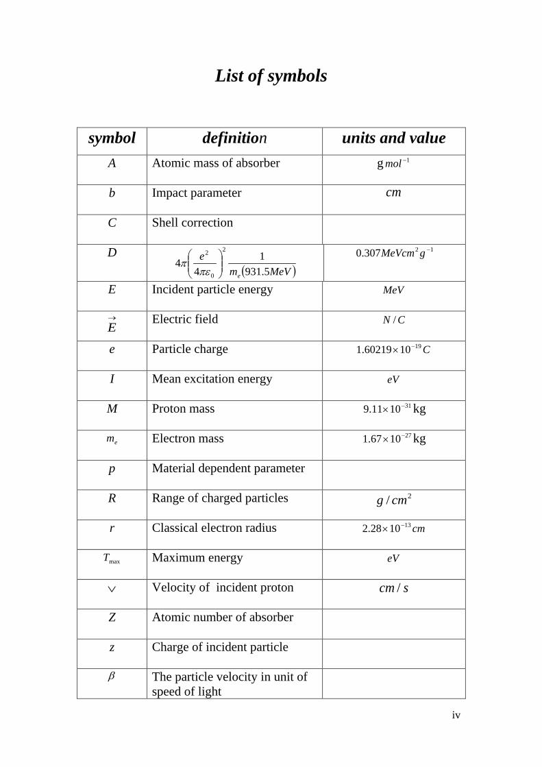
List of symbols
symbol definition units and value A Atomic mass of absorber
g 1−mol
b Impact parameter
cm
C Shell correction
D ( )MeVm
e
e 5.9311
44
2
0
2
πε
π 12307.0 −gMeVcm
E Incident particle energy
MeV
→
E Electric field
CN /
e Particle charge
C1910 1.60219 −×
I Mean excitation energy
eV
M Proton mass
311011.9 −× kg
em Electron mass
271067.1 −× kg
p Material dependent parameter
R Range of charged particles
2/ cmg
r Classical electron radius
cm131028.2 −×
maxT Maximum energy
eV
∨ Velocity of incident proton
scm /
Z Atomic number of absorber
z Charge of incident particle
β The particle velocity in unit of speed of light
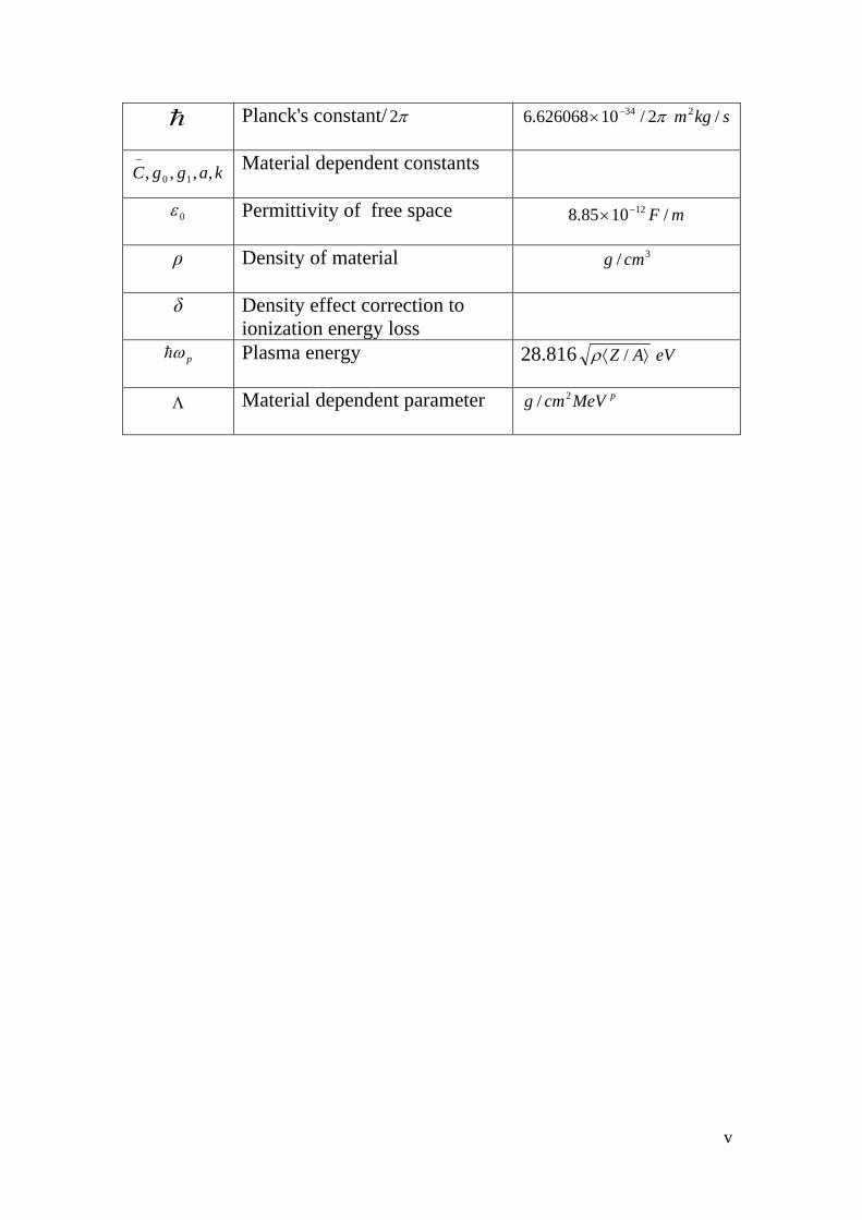
v
Planck's constant/ π2
π2/10626068.6 34−× skgm /2
kaggC ,,,, 10
−
Material dependent constants
0ε Permittivity of free space
mF /1085.8 12−×
ρ Density of material
3/ cmg
δ Density effect correction to ionization energy loss
pω Plasma energy
28.816 ⟩⟨ AZ /ρ eV
Λ Material dependent parameter
pMeVcmg 2/

vi
List of Figures
Page Explain Figure
No. 6 Interaction of a heavy charged particle with an electrons
in a target atom. 2.1
7 Interaction of a heavy charged particle with a nucleus.
2.2
9 The approximate trajectory of a fast particle passing a 'rest' particle.
2.3
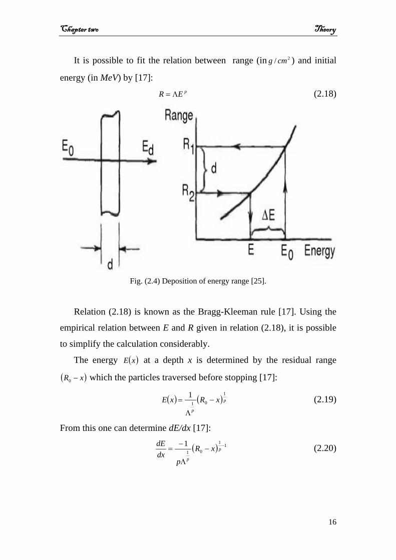
16 Deposition of energy range.
2.4
17 The experimental results of energy loss for protons.
3.1
18 The calculated results of energy loss for different materials.
3.2
19 Published theoretical stopping power for protons in Cu with exact maxT and approximate maxT .
3.3
20 The effect of maxT on the energy loss of an incident protons on C as a function of βγ .
3.4
20 The effect of maxT on the energy loss of an incident protons on C as a function of initial energy.
3.5
21 The same as Fig. (3.4) but for Al.
3.6
21 The same as Fig. (3.5) but for Al.
3.7
22 The same as Fig. (3.4) but for Cu.
3.8
22 The same as Fig. (3.5) but for Cu.
3.9
23 The same as Fig. (3.4) but for water.
3.10
23 The same as Fig. (3.5) but for water.
3.11
24 The effect of density correction on the relation between energy loss of incident protons and βγ for C.
3.12
25 The effect of density correction on the relation between energy loss of incident protons and energy for C.
3.13
vii
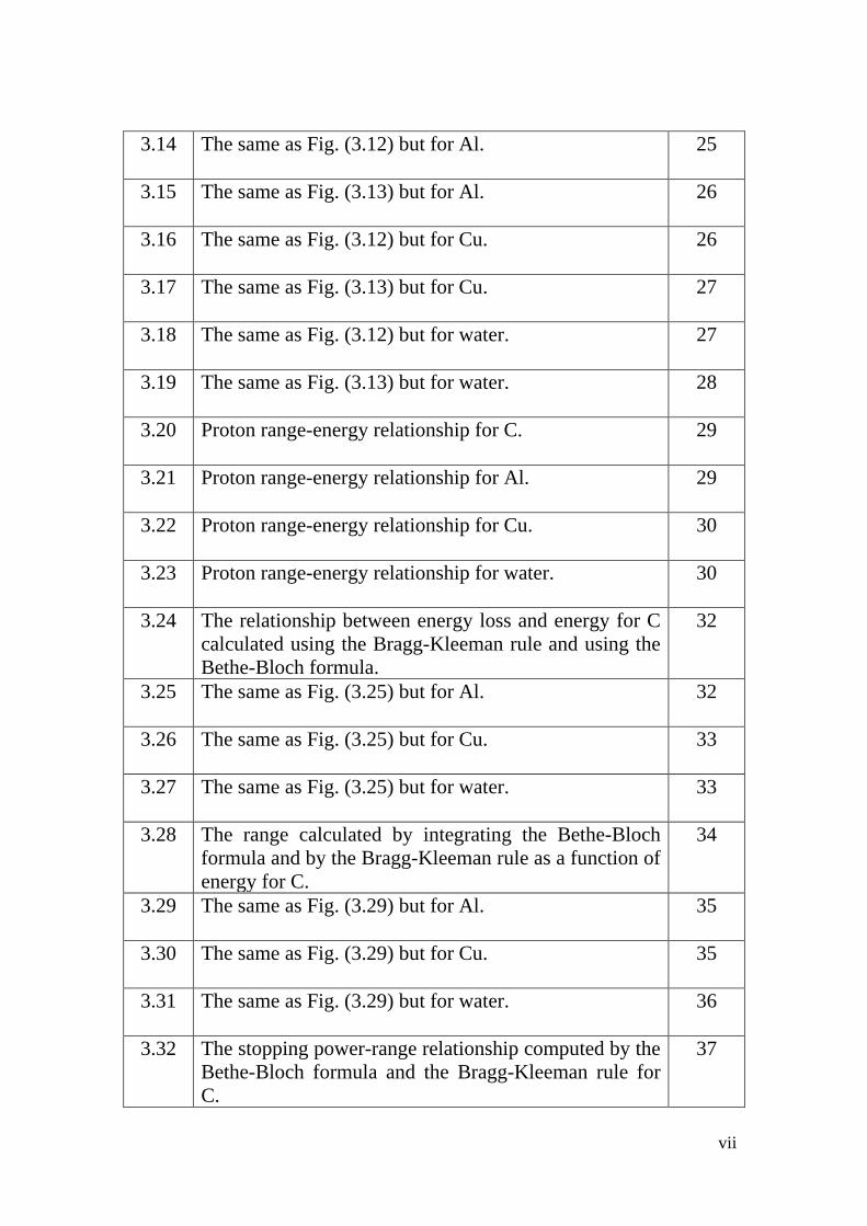
25 The same as Fig. (3.12) but for Al.
3.14
26 The same as Fig. (3.13) but for Al.
3.15
26 The same as Fig. (3.12) but for Cu.
3.16
27 The same as Fig. (3.13) but for Cu.
3.17
27 The same as Fig. (3.12) but for water.
3.18
28 The same as Fig. (3.13) but for water.
3.19
29 Proton range-energy relationship for C.
3.20
29 Proton range-energy relationship for Al.
3.21
30 Proton range-energy relationship for Cu.
3.22
30 Proton range-energy relationship for water.
3.23
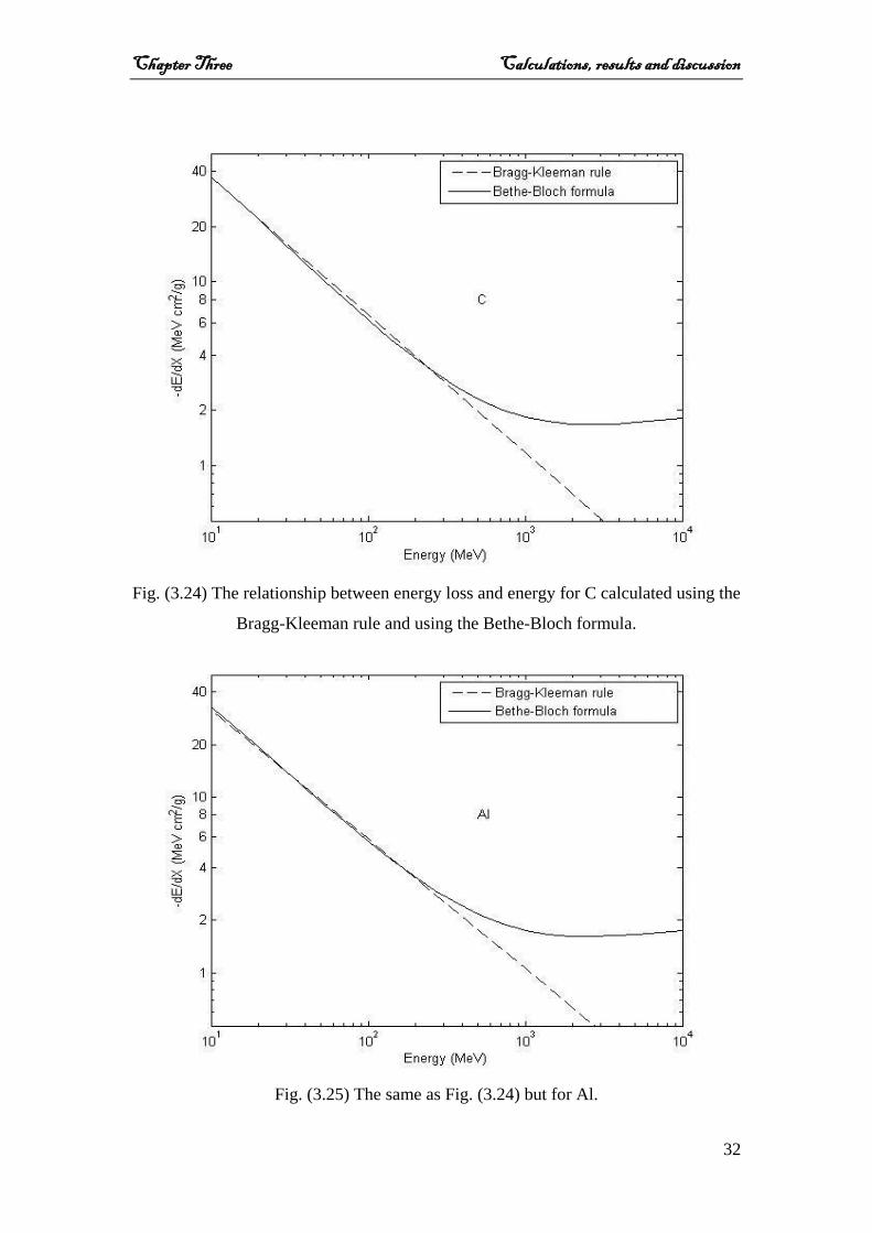
32 The relationship between energy loss and energy for C calculated using the Bragg-Kleeman rule and using the Bethe-Bloch formula.
3.24
32 The same as Fig. (3.25) but for Al.
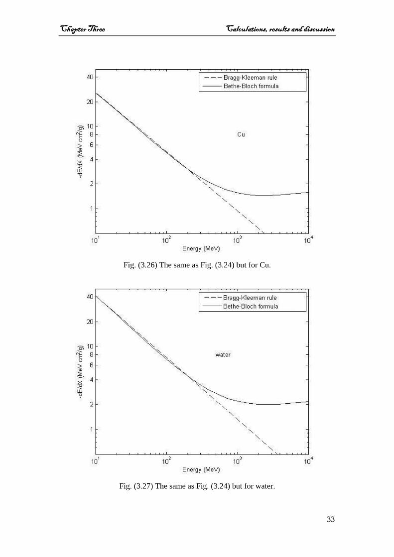
3.25
33 The same as Fig. (3.25) but for Cu.
3.26
33 The same as Fig. (3.25) but for water.
3.27
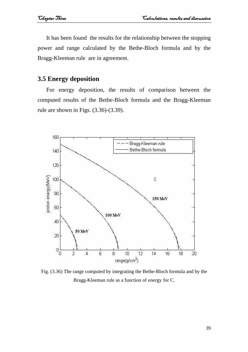
34 The range calculated by integrating the Bethe-Bloch formula and by the Bragg-Kleeman rule as a function of energy for C.
3.28
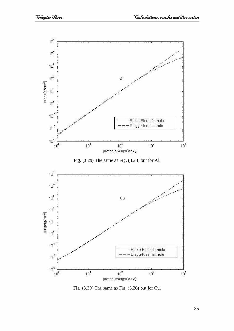
35 The same as Fig. (3.29) but for Al.
3.29
35 The same as Fig. (3.29) but for Cu.
3.30
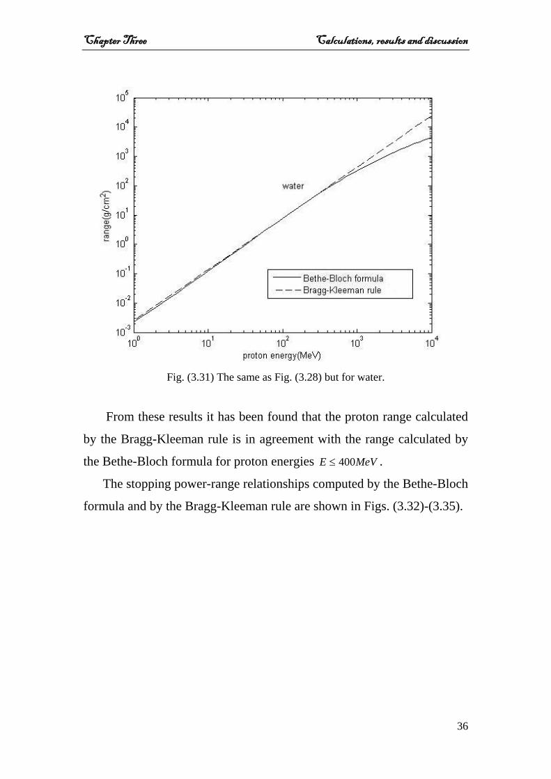
36 The same as Fig. (3.29) but for water.
3.31
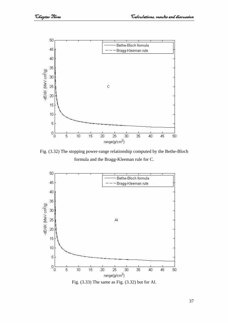
37 The stopping power-range relationship computed by the Bethe-Bloch formula and the Bragg-Kleeman rule for C.
3.32
viii
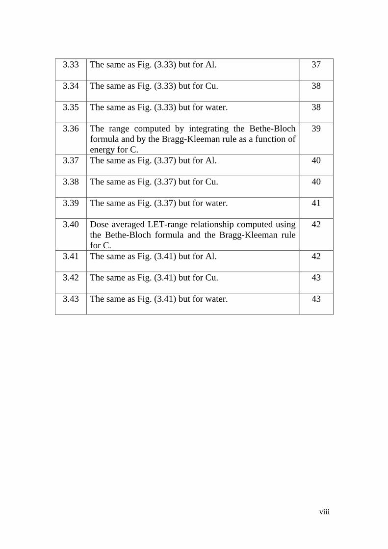
37 The same as Fig. (3.33) but for Al.
3.33
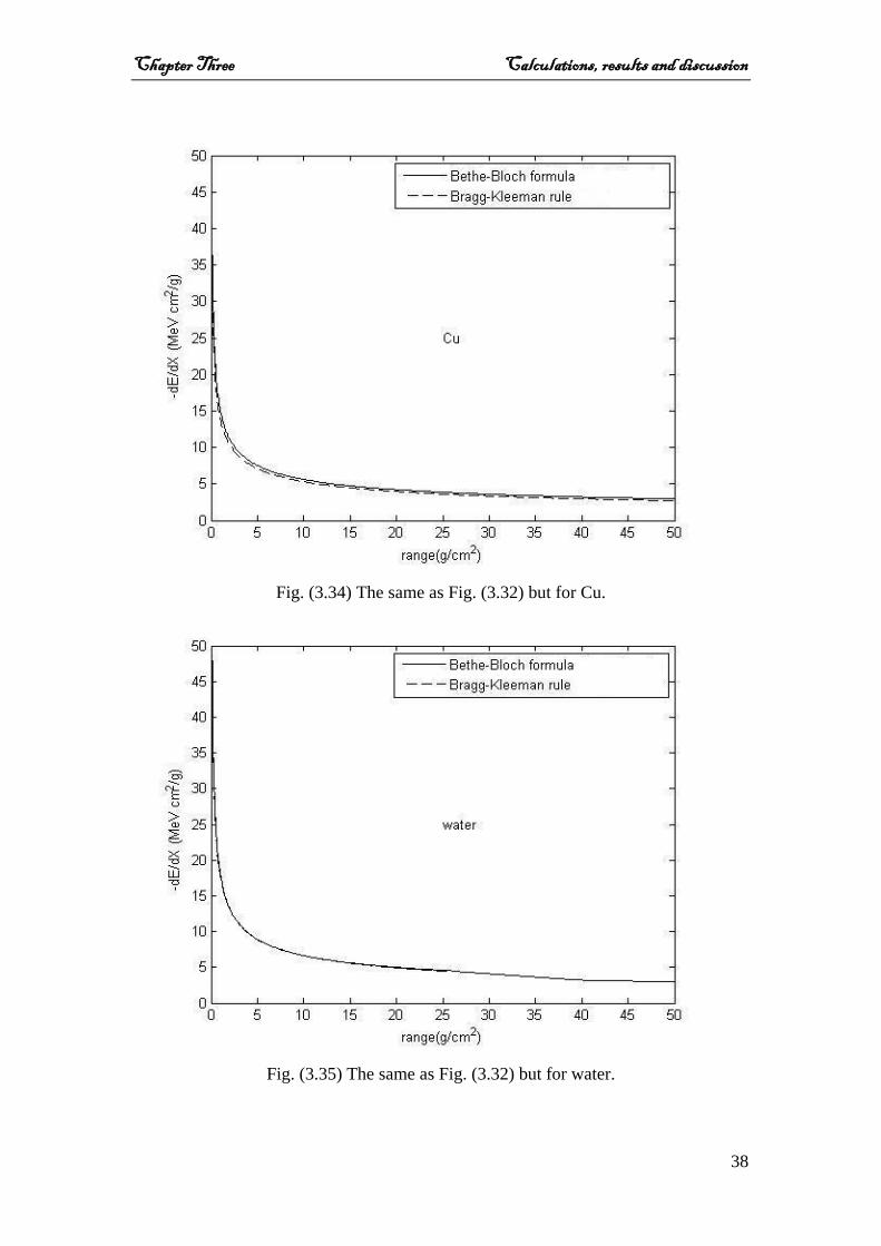
38 The same as Fig. (3.33) but for Cu.
3.34
38 The same as Fig. (3.33) but for water.
3.35
39 The range computed by integrating the Bethe-Bloch formula and by the Bragg-Kleeman rule as a function of energy for C.
3.36
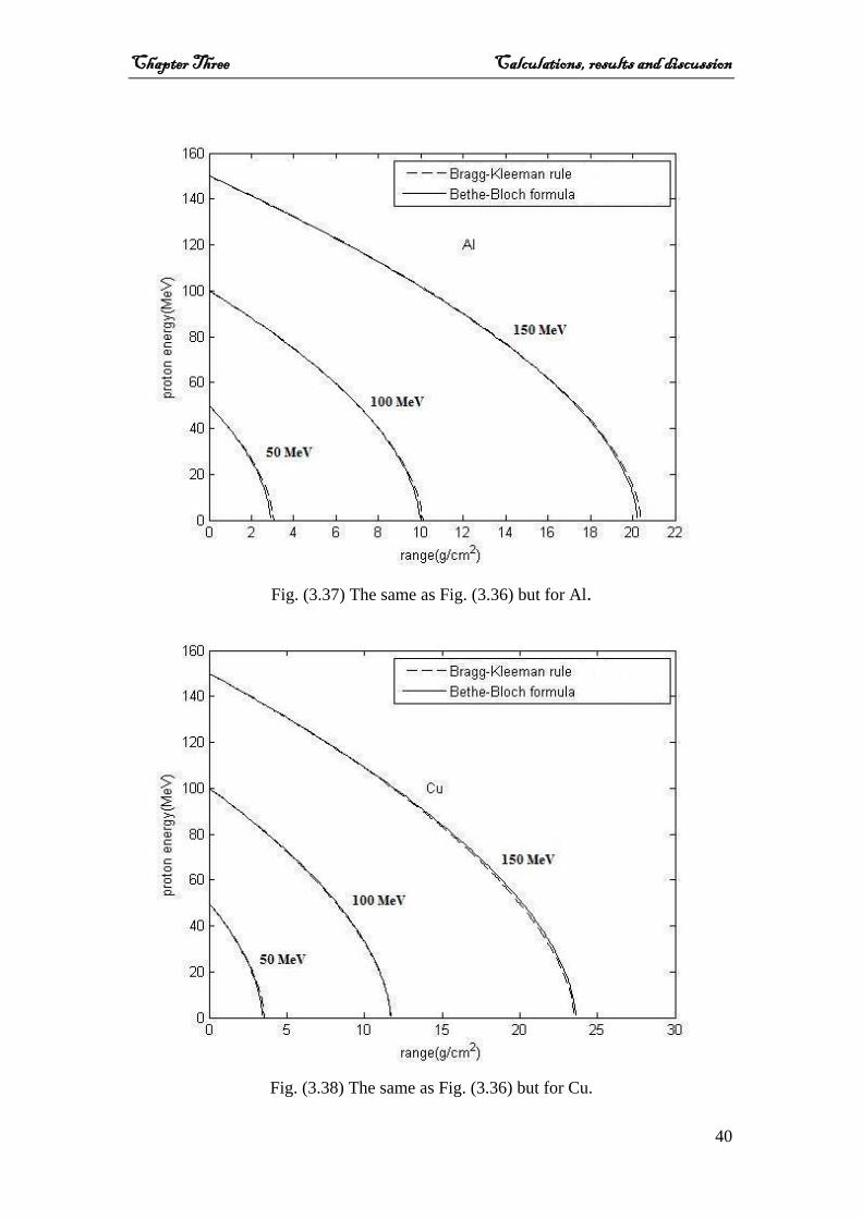
40 The same as Fig. (3.37) but for Al.
3.37
40 The same as Fig. (3.37) but for Cu.
3.38
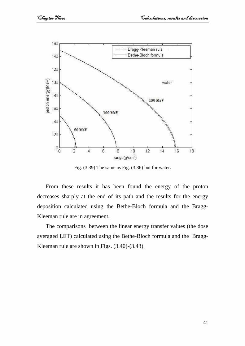
41 The same as Fig. (3.37) but for water.
3.39
42 Dose averaged LET-range relationship computed using the Bethe-Bloch formula and the Bragg-Kleeman rule for C.
3.40
42 The same as Fig. (3.41) but for Al.
3.41
43 The same as Fig. (3.41) but for Cu.
3.42
43 The same as Fig. (3.41) but for water.
3.43

Chapter one
Introduction and
historical survey
Chapter one Introduction and historical survey
1
1.1 Introduction The study of the passage of charged particles through matter is one of
basic importance for modern physics. Also, the knowledge of the
interactions that take place in the passage of charged particles allowed
possible to develop several detectors [1].
Stopping power is the energy loss of a particle per unit path length in
a particular medium [2]. It is specified by the quantity –dE/dx, where -dE
is the energy loss and dx is the increment of the path length. The spatial
distribution of energy deposition in the particle track is described by the
Linear Energy Transfer (LET), or the amount of energy actually
deposited per unit length along the path [2].
To determine the dose at any point due to charged particle irradiations
it is necessary to know, not only the fluency, but also the charged
particles energy and to use this to calculate the stopping power at that
point [3]. Heavy charged particles are of interest in radiation therapy
because of several distinct physical properties. As these charged particles
pass through a medium, their rate of energy loss or specific ionization
increases with decreasing particle velocity [4]. Electron and proton
radiations are used extensively for medical purposes in diagnostic and
therapeutic procedures [5].
The macroscopic dose of a particle beam is given by the number of
particles traversing the unit mass and the dose deposited by each particle,
called linear energy transfer (LET). This energy deposition of heavy
charged particles, like protons or heavier ions, can be described by the
Bethe-Bloch formula [6]. The dose average LET is considered as
a00000000000000 measure of the radiation quality [7].

Chapter one Introduction and historical survey
2
1.2 Historical survey In 1965, R. W. Peele [8] studied the method that was used to achieve
rapid computing in a digital computer of the specific energy loss of
energetic charged particles. The computation were based on the use of the
usual Bethe-Bloch formula with a density effect correction which might
be required for incident proton energies as high as 1GeV.
In 1976, W. R. Nelson [9] explained the importance of radiation
dosimeters in medicine to treat cancer and the theoretical relations to
compute the stopping power.
In 1993, Don Groom [10] worked on copper to study the first
correction of the Bethe-Bloch formula (maximum energy transfer to
electrons) and its effect on the results.
In 1994, Douglas J. Wagenaar [11] explained that γ-rays, X-rays,
neutrons and neutrinos all have no net charge, they are electrostatically
neutral, so in order to detect them, they must interact with matter and
produce an energetic charged particle. In the case of gamma and X-rays, a
photo-electron is produced. In the case of neutrons, a proton is given
kinetic energy in a billiard ball collision. So, he discussed charged
particle interactions by demonstrating that even when detecting neutral
particles one must think in terms of the charged particles.
In 1997, H Tai, Hans Bishel, John W. Wilson, Judy L. Shinn, Francis
A. Cucinotta and Francis F. Badavi [12] studied the Bethe-Bloch formula
to calculate stopping power and range. They put this formula in the form
of a computer program to calculate electronic stopping power for
protons, α particles and other ions.
Also in 1997, B. Vankuik, G. Gardener, S. Bellavia, A. Rusek and K.
Brown [13] studied the most important relations which are used to
Chapter one Introduction and historical survey
3
compute the energy loss and the computer programs which are used to
compute the stopping power.
In 1999, J. F. Ziegler [14] studied all equations used for calculating
the stopping power and the accuracy for different element materials. The
theory of energetic ion stopping was reviewed with emphasis on those
aspects of relevance to the calculation of accurate stopping powers
(corrections).
In 1999, John C. Armitage, Madhu S. Dixit, Jacques Dubeau, Hans
Mes and F. Gerald Oakham [15] studied the interaction of charged
particles, such as electrons and heavy charged particles, with different
elements (silicon, argon and gold). They measured the energy losses and
the ranges of the particles in these elements.
In 1999, P. T. Leung [16] worked on the density correction of the
Bethe-Bloch stopping power theory for heavy target elements. He worked
on the relativistic Bethe-Bloch stopping power formula. This relativistic
correction was found to be significant for high-Z target atoms and
relatively high-energy incident particles.
In 2000, Luigi Foschini [1] studied the most important stages in the
development of the theory behind the stopping power formula. He started
with Ernest Rutherford in September 1895 and his recognized two
different kinds of radiations emitted by uranium to year 1998 and
referred to everyone who contributed to the development of the stopping
power theory.
In 2004, Jan Jakob Wilkens [7] developed a fast algorithm for three-
dimensional calculations of the dose-averaged linear energy transfer
(LET) . He studied stopping power in terms of dose averaged LET, range
and dose for protons.
Chapter one Introduction and historical survey
4
In 2004, H.W. den Hartog and D.I. Vainshtein [17] calculated the
energy loss in a thick target for 0.1 MeV -3 MeV electron irradiation. He
calculated the range using the Bethe-Bloch formula and the Bragg-
Kleeman rule for NaCl, water and aluminum.
In 2006, P. Sigmund and A. Schinner [18] studied the shell
correction to the stopping power for protons within the first Born
approximation in both a non relativistic and a relativistic version of this
approximation.
In 2006, M. F. Zaki, A. Abdel-Naby and Ahmed Morsy [19] studied
the theoretical and experimental investigations of the penetration of
charged particles in matter using solid state nuclear track detectors. An
attempt has been made to examine the suitability of the single-sheet
particle identification technique in CR-39 and CN-85 polycarbonate. The
ranges of the ions ( He4 , Kr86 and Nb93 ) in these detectors have also been
computed theoretically.
In 2006, Önder Kabadayi [20] calculated the range of protons and
alpha particles in NaI, which is a commonly used compound in
scintillation detector manufacturing. The stopping power of protons and
alpha particles in NaI was calculated first by using a theoretical
formulation.
In 2006, F. Maas [21] worked on the interaction of particles with
matter and the importance of computing the density correction in the
Bethe-Bloch formula with particle energy above 1GeV.
1.3 The aim of the present work The aim of the present work is to calculate the stopping power and
range using the Bethe-Bloch formula and the Bragg-Kleeman rule for
Chapter one Introduction and historical survey
5
protons passing through carbon, aluminum, copper and water with
different energies and studying different parameters affecting the
stopping power.
1.4 The structure of the rest of the thesis The rest of the thesis is organized as follows:
Chapter two contains the theoretical formulation of the stopping
power and corrections.
Chapter three contains the calculation of stopping power and range
using the Bethe-Bloch formula with maximum energy and density
correction, and using the Bragg-Kleeman rule and the discussion of the
comparison between the two kinds of calculations.
Chapter four contains the conclusions of this work and
recommendations for future work.
Chapter Two
Theory
Chapter two Theory
6
2.1 Interaction of charged particles with matter
Charged particles such as protons, alpha particles, and fission
fragment ions are classified as heavy, being much more massive than the
electron. For a given energy, their speed is lower than that of an electron,
but their momentum is greater and they are less readily deflected upon
collision. The mechanism by which they slow down in matter is mainly
electrostatic interaction with the atomic electrons and with nuclei. In each
case the Coulomb force, varying as 1/ 2r with distance of separation r,
determines the result of a collision [22].
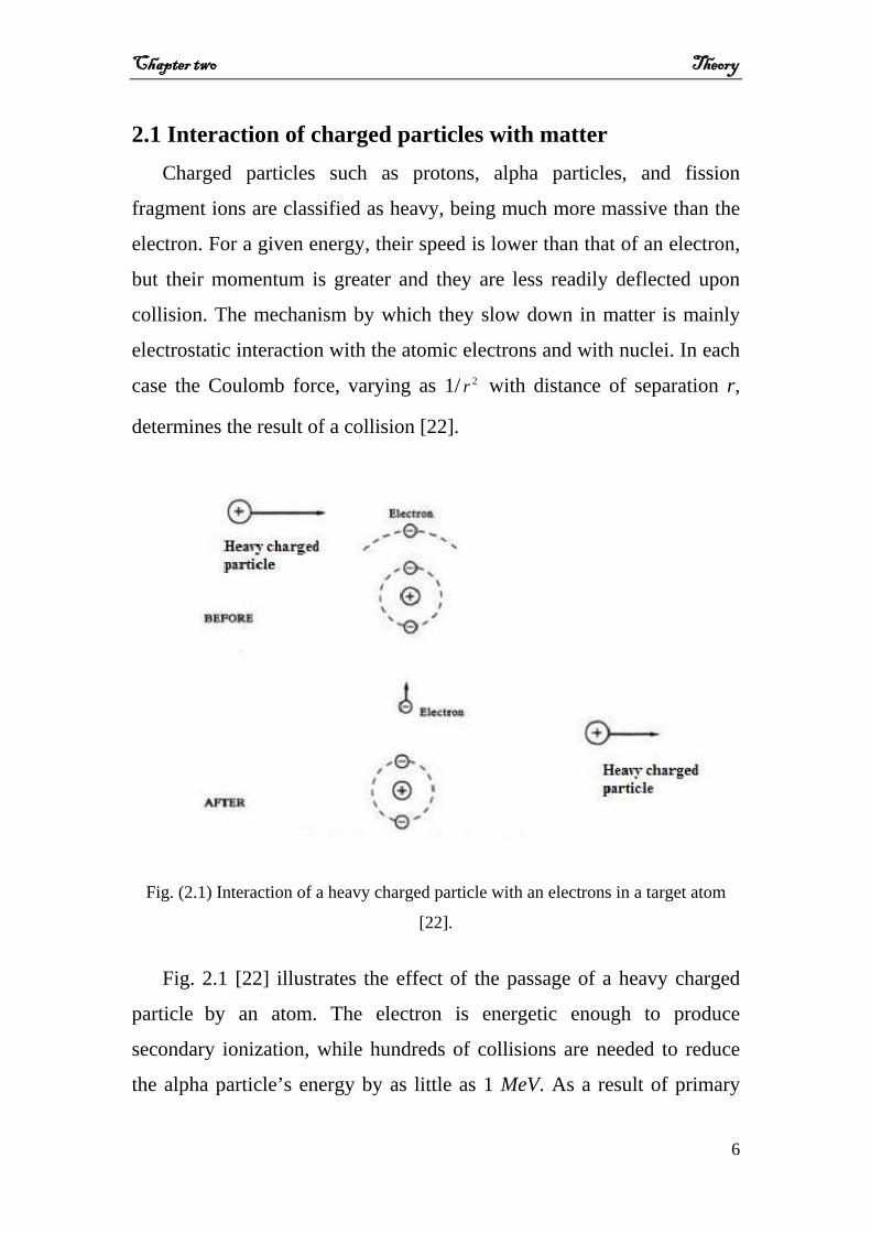
Fig. (2.1) Interaction of a heavy charged particle with an electrons in a target atom
[22].
Fig. 2.1 [22] illustrates the effect of the passage of a heavy charged
particle by an atom. The electron is energetic enough to produce
secondary ionization, while hundreds of collisions are needed to reduce
the alpha particle’s energy by as little as 1 MeV. As a result of primary
Chapter two Theory
7
and secondary processes, a great deal of ionization is produced by heavy
charged particles as they move through matter. In contrast, when a heavy
charged particle comes close to a nucleus, the electrostatic force causes it
to move in a hyperbolic path as in Fig. (2.2) [22]. The projectile is
scattered through an angle that depends on the detailed nature of the
collision, i.e., the initial energy and direction of motion of the incoming
ion relative to the target nucleus, and the magnitudes of electric charges
of the interacting particles. The charged particle looses a significant
amount of energy in the process, in contrast with the slight energy loss on
collision with an electron. Unless the energy of the bombarding particle is
very high and it comes within the short range of the nuclear force, there is
a small chance that it can enter the nucleus and cause a nuclear reaction.
A measure of the rate of ion energy loss with distance traveled is the
stopping power, symbolized by -dE/dx. It is also known as the linear
energy transfer (LET) [22].
Fig. (2.2) Interaction of a heavy charged particle with a nucleus [22].
Chapter two Theory
8
2.2 Stopping power For charged particles of energy < 10 MeV, the dominant mechanism
for energy loss is the excitation or ionization of the atoms (or molecules)
of the gas: electrons being excited to higher bound energy levels in the
atom, or detached completely. The essential physics of the process may
be understood using classical mechanics.
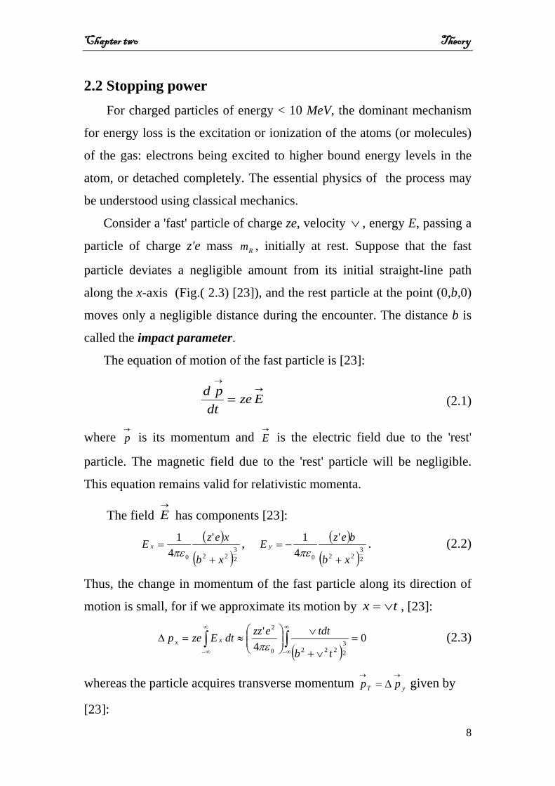
Consider a 'fast' particle of charge ze, velocity ∨ , energy E, passing a
particle of charge z'e mass Rm , initially at rest. Suppose that the fast
particle deviates a negligible amount from its initial straight-line path
along the x-axis (Fig.( 2.3) [23]), and the rest particle at the point (0,b,0)
moves only a negligible distance during the encounter. The distance b is
called the impact parameter.
The equation of motion of the fast particle is [23]:
→
→
= Ezedt
pd (2.1)
where →
p is its momentum and →
E is the electric field due to the 'rest'
particle. The magnetic field due to the 'rest' particle will be negligible.
This equation remains valid for relativistic momenta.
The field →
E has components [23]:
( )( )2
3220
'4
1
xb
xezE x
+=
πε, ( )
( )23
220
'4
1
xb
bezE y
+−=
πε. (2.2)
Thus, the change in momentum of the fast particle along its direction of
motion is small, for if we approximate its motion by tx ∨= , [23]:
( )
04
'
23
2220
2
=∨+
∨
≈=∆ ∫∫
∞
∞−
∞
∞− tb
tdtezzdtEzep xx πε (2.3)
whereas the particle acquires transverse momentum yT pp→→
∆= given by
[23]:
Chapter two Theory
9
Fig. (2.3) The approximate trajectory of a fast particle passing a 'rest' particle [23].
( ) ∨
−=
∨+
−== ∫∫
∞
∞−
∞
∞− bezz
tb
bdtezzdtEzep yT2
4'
4'
0
2
23
2220
2
πεπε. (2.4)
(The integral is easily evaluated by the substitution φtanbt =∨ .)
Since momentum is conserved overall, the 'rest' particle acquires
momentum ( )Tp− and assuming that it does not attain a relativistic
velocity, gains kinetic energy )2/( 2RT mp . This energy must be lost by the
fast particle [23]:
RR
T
mbezz
mpE 22
2
0
22 14
'22 ∨
−=−=∆
πε. (2.5)
Note that ΔE does not depend on the mass of the fast particle, and that
the calculation is valid for relativistic particles [23].
In applying this result, the 'rest' particles are the atomic nuclei and
atomic electrons of the gas. For an atomic nucleus of atomic number Z,
z' = Z, and (except for hydrogen) pR Zmm 2≈ . For an electron z' 1−= and
Chapter two Theory
10
eR mm = . Using the formula (2.5), when a fast charged particle passes
through a gas the ratio of energy lost to the atomic electrons, to the
energy lost to the atomic nuclei, is 3104/2 ×≈≈ ep mm (since each atom has
Z electrons). Thus the energy lost to the nuclei is negligible compared
with that lost to the electrons [23].
If the gas is of mass density ρ, and consists of atoms of atomic
number Z, then the fast particle moves through a distance dx in the gas
passing, on average, ( )am/ρ Z2π b db dx electrons with impact parameter
between b and b + db, and the energy lost to these electrons is [23]:
dxbdb
mmZzeEd
ea2
2
0
22 1
44
∨
−=
ρπε
π . (2.6)
Integrating this expression over all impact parameters between minb
and maxb , the total rate of energy loss along the path, or stopping power, is
[23]:
LmmZze
dxdE
ea2
2
0
2 14
4∨
=−
ρπε
π , (2.7)
where ( )minmax /ln bbL = .
Since Ama ≈ atomic mass units, where A is the mass number of the
atom, one can write [23]:
LzcAZD
dxdE 2
∨
=− ρ (2.8)
where
( ) 307.05.931
14
42
0
2
=
=
MeVmeD
eπεπ 12 −gMeVcm .
and the mass density ρ of the material is expressed in g 3−cm [23].
Formula (2.5) clearly breaks down for small b, since the energy
transfer cannot be indefinitely large; it also breaks down at large b, since
to ionize the atom the energy transfer cannot be indefinitely small. A
Chapter two Theory
11
quantum mechanical calculation by Bethe and Bloch which holds for
charged particles other than electrons and positrons gives equation (2.8)
with [23]
−
⟩⟨
= 22222
ln ββγ
Icm
L e , (2.9)
where ⟩⟨I is a suitably defined average ionization energy for atomic
electrons, 2
22
c∨
=β , and 21
1β
γ−
= [23].
A better parameterization of I is given by [10]:
712 += ZI eV for 1 < Z < 13
19.08.5876.9 −+= ZZI eV for Z ≥ 13
In the ‘minimum ionization’ region where 43−=βγ , the minimum
value of dxdE /− can be calculated from eq. (2.8) and, for a particle with
unit charge, is given approximately by [24]:
21
min
5.3 cmMeVgAZ
dxdE −≈
− (2.10)
Ionization losses are proportional to the squared charge of the
particle, so that a fractionally charged particle with 3≥βγ would have a
much lower rate of energy loss than the minimum energy loss of any
integrally charged particle [24].
2.3 Maximum energy One is concerned with the average energy loss of a high-energy
massive charged particle. High energy means that the velocity is high
compared with that of atomic electrons, and massive mean that the
particle is not an electron or positron, but a heavier particle. Most
particles of interest have charge e± [10].

Chapter two Theory
12
At low energies, nuclear recoil contributes to energy loss. At very
high energies ( above 100 GeV ) radiative processes contribute in
significant way and eventually dominate. Here, one is concerned with the
middle regime in which virtually all of the energy loss occurs via a large
number of collisions with electrons in the medium. In this discussion the
medium is taken as a pure element with atomic number Z and atomic
mass A, but this restriction can easily be removed [10].
The mean energy loss rate ( -dE/dx or stopping power S ) is, therefore,
calculated by summing the contributions of all possible scatterings.
These are normally scatterings from a lower to higher state, so that the
particle looses a small amount of energy in each scattering. The kinetic
energy of the scattering electron is T, and the magnitude of the 3-
momentum transfer is q [10].
1. Low-T approximation. Here q/ (roughly an impact parameter b )
is large compared with atomic dimensions. The scattered electrons
have kinetic energies up to some cutoff 1T , and the contribution to
the stopping power is [10]:
−+= 22
2221
22
1 ln2/
ln12
βγββ cmI
TAZzDS
e
, (2.11)
where the denominator 22 2/ ∨emI in the first term is the effective
lower cutoff on the integral of dT/T. The first term comes from
''longitudinal excitations'' (the ordinary Coulomb potential), and the
other two terms from transverse excitations. The low-T region is
associated with large impact parameters and, hence, with long
distance. The correction is usually introduced by subtracting a
separate term called density correction δ [10].
Chapter two Theory
13
2. Intermediate-T approximation. In this region, atomic excitation
energies are not small compared with T, but, in contrast to the low-
T region, transverse excitation can be neglected. This region
extends from 1T to 2T , and the contribution to –dE/dx is [10]:
=
1
22
22 ln
2 TTZzDS
β. (2.12)
3. High-T approximation. In this region one can equate T with the
energy of the electron, i. e., neglect its binding energy. When the
energy is carried out between the lower limit 2T (which is
hopefully the same as in eq. (2.12)) and the upper limit upperT , one
obtains [10]:
−=
max
2
22
23 ln1
2 TT
TT
AZzDS upperupper ββ
. (2.13)
Here, maxT is the maximum possible electron recoil kinetic energy,
given by [10]:
2
222
max
21
2
++
=
Mm
Mmcm
Tee
e
γ
γβ . (2.14)
where M is the mass of the charged particle.
upperT is normally equal to maxT . In any case, maxTTupper ≤ . The low-
energy approximation 222max 2 γβcmT e≈ is implicit. The minimum T in this
region, 2T , is much less than 2cme but much larger than (any) electron's
binding energy –a situation that becomes a little paradoxical for high-Z
material. The "shell correction" which corrects this problem is usually
introduced as a term -2C/Z inside the square brackets of eq. (2.13). The
high-T region is associated with high-energy recoil particles. For the
usual case maxTTupper = , the second term is virtually constant, while the first
term rises as 2lnγ . If the maximum energy transfer is limited to some

Chapter two Theory
14
maxTTupper < , then the increase disappears. In the above, it was implicitly
assumed that one can find electron kinetic energies 1T and 2T at which the
three regions join. When the three contributions are summed the
intermediate T’s cancel and one gets the usual Bethe-Bloch formula, [10]:
−−−
=−
22
ln211 2
2max
222
22 δβ
γββ Z
CI
TcmAZDz
dxdE e (2.15)
where δ is the density correction
2.4 Shell correction The shell correction becomes important only at the lowest energy.
This correction is, therefore, not of much interest in high-energy physics
applications. It treats effects at very low particle momentum when the
particle velocity is comparable or lower than the orbital velocity of the
bound atomic electrons [10].
2.5 Density correction
As the particle energy increases its electric field increases flattens and
extends, so that the distant-collision contribution to the energy loss
increases as ( ) 2/1ln/ln2/ −+= βγωδ Ip [10]. Here Mcp /=βγ is the
particle momentum in terms of its mass, pω is the so-called plasma
energy, parameterized as 28.816 ⟩⟨ AZ /ρ eV. The term with ( )Ip /ln ω
accounts for the polarizability of the medium. However, this
parameterization of the density correction is only valid at large βγ . For
electrons, this parameterization is valid almost always. For charged
particles, however, a parameterization is necessary and it is given in the
following form [10]:
Chapter two Theory
15
=δ ( )
−+−
−−
−
0)10(ln2
)10(ln2
1kggaCg
Cg
)(
)()(
0
10
1
ggifgggif
ggif
<<≤
≥
; (2.16)
Here, βγ10log=g , ( )( ).1/ln2−
+−= pIC ω aggC ,,, 10
−
and k are material
dependent constants. 0g is usually around zero. Values of k range
between 2.9 and 3.6. The value of a is chosen such that it provides a
smooth passage from 0gg < to 1gg > [10].
In order to parameterize this in a simple way, a general
parameterization for all materials was chosen: 00 =g , 31 =g , 3=k and
27/0Ca −= [10].
2.6 The range The range of the charged particles R in a medium can be determined
by integrating the stopping power from 0 to E [12]:
dEdxdER
E 1
0
−
∫
−= (2.17)
In practice, however, not all charged particles that start with the same
energy will have the same range [12].
The range, as given by eq. (2.17), is actually an average value because
scattering is a statistical process and there will, therefore, be a spread of
values for individual particles. The spread will be greater for light
particles and smaller for heavier particles. These properties have
implications for the use of radiation in therapeutic situations, where it
may be necessary to deposit energy within a small region at a specific
depth of tissue, for example to precisely target a cancer [24]. Fig.(2.4)
shows a deposition of energy range diagram [25].
Chapter two Theory
16
It is possible to fit the relation between range (in 2/ cmg ) and initial
energy (in MeV) by [17]: pER Λ= (2.18)
Fig. (2.4) Deposition of energy range [25].
Relation (2.18) is known as the Bragg-Kleeman rule [17]. Using the
empirical relation between E and R given in relation (2.18), it is possible
to simplify the calculation considerably.
The energy ( )xE at a depth x is determined by the residual range
( )xR −0 which the particles traversed before stopping [17]:
( ) ( ) p
p
xRxE1
01
1−
Λ
= (2.19)
From this one can determine dE/dx [17]:
( ) 11
01
1 −−
Λ
−= p
p
xRp
dxdE (2.20)

Chapter Three
Calculations, results and discussion
Chapter Three Calculations, results and discussion
17
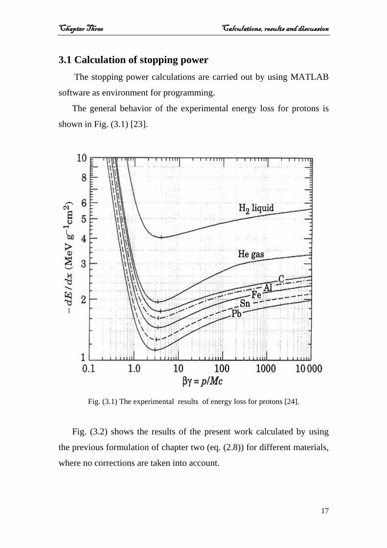
3.1 Calculation of stopping power The stopping power calculations are carried out by using MATLAB
software as environment for programming.
The general behavior of the experimental energy loss for protons is
shown in Fig. (3.1) [23].
Fig. (3.1) The experimental results of energy loss for protons [24].
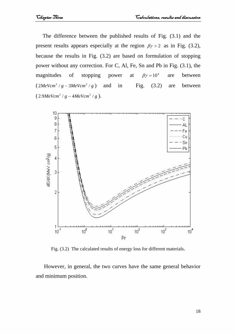
Fig. (3.2) shows the results of the present work calculated by using
the previous formulation of chapter two (eq. (2.8)) for different materials,
where no corrections are taken into account.
Chapter Three Calculations, results and discussion
18
The difference between the published results of Fig. (3.1) and the
present results appears especially at the region 2>βγ as in Fig. (3.2),
because the results in Fig. (3.2) are based on formulation of stopping
power without any correction. For C, Al, Fe, Sn and Pb in Fig. (3.1), the
magnitudes of stopping power at 410=βγ are between
( gMeVcmgMeVcm /3/2 22 − ) and in Fig. (3.2) are between
( gMeVcmgMeVcm /4/9.2 22 − ).
Fig. (3.2) The calculated results of energy loss for different materials.
However, in general, the two curves have the same general behavior
and minimum position.
Chapter Three Calculations, results and discussion
19
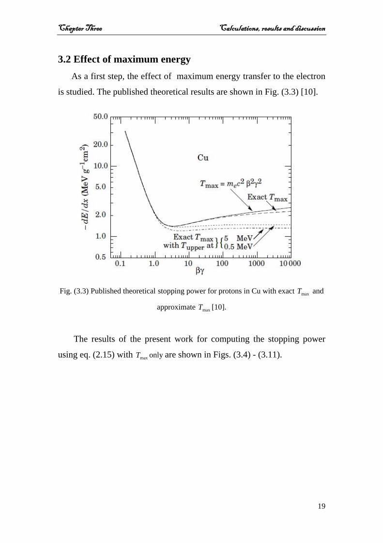
3.2 Effect of maximum energy As a first step, the effect of maximum energy transfer to the electron
is studied. The published theoretical results are shown in Fig. (3.3) [10].
Fig. (3.3) Published theoretical stopping power for protons in Cu with exact maxT and
approximate maxT [10].
The results of the present work for computing the stopping power
using eq. (2.15) with maxT only are shown in Figs. (3.4) - (3.11).
Chapter Three Calculations, results and discussion
20
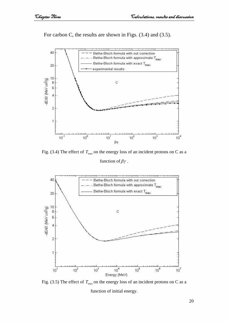
For carbon C, the results are shown in Figs. (3.4) and (3.5).
Fig. (3.4) The effect of maxT on the energy loss of an incident protons on C as a
function ofβγ .
Fig. (3.5) The effect of maxT on the energy loss of an incident protons on C as a
function of initial energy.
Chapter Three Calculations, results and discussion
21
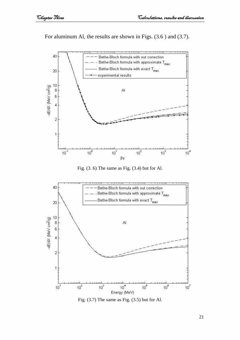
For aluminum Al, the results are shown in Figs. (3.6 ) and (3.7).
Fig. (3. 6) The same as Fig. (3.4) but for Al.
Fig. (3.7) The same as Fig. (3.5) but for Al.
Chapter Three Calculations, results and discussion
22
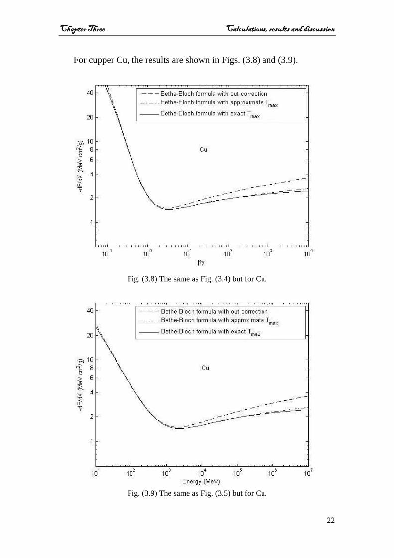
For cupper Cu, the results are shown in Figs. (3.8) and (3.9).
Fig. (3.8) The same as Fig. (3.4) but for Cu.
Fig. (3.9) The same as Fig. (3.5) but for Cu.
Chapter Three Calculations, results and discussion
23
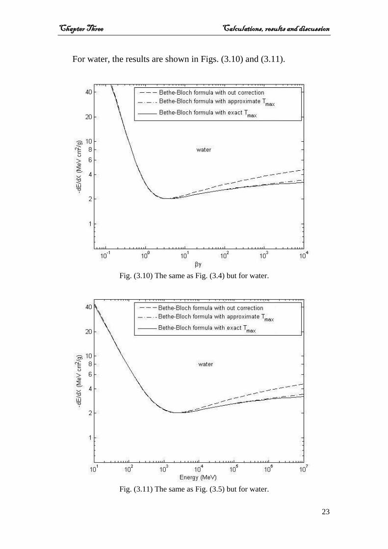
For water, the results are shown in Figs. (3.10) and (3.11).
Fig. (3.10) The same as Fig. (3.4) but for water.
Fig. (3.11) The same as Fig. (3.5) but for water.
Chapter Three Calculations, results and discussion
24
It has been found that the effect of the maximum energy appears at
200≥βγ ( MeV5102× ) and the results are coincident with the published
theoretical data in Fig. (3.3), but with a small difference relative to the
experimental results at 200≥βγ . This reflects the importance of
computing the stopping power with maximum energy to lower the
difference between theoretical and experimental results in this region.
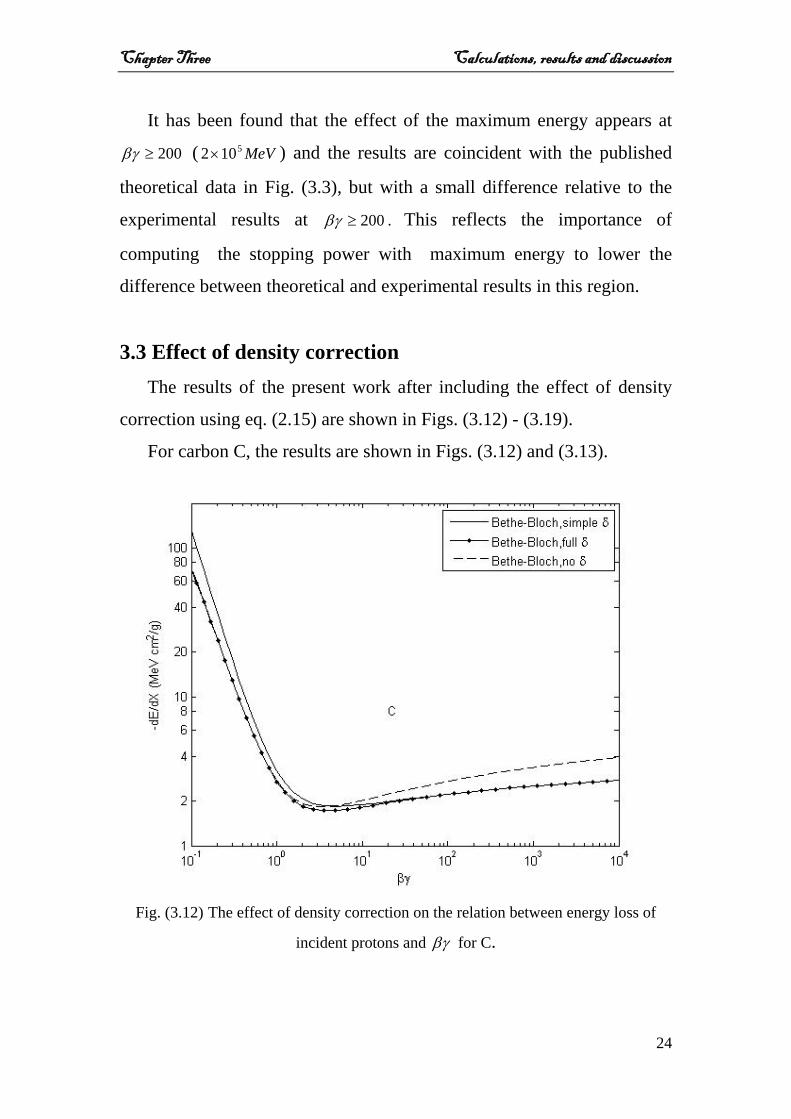
3.3 Effect of density correction The results of the present work after including the effect of density
correction using eq. (2.15) are shown in Figs. (3.12) - (3.19).
For carbon C, the results are shown in Figs. (3.12) and (3.13).
Fig. (3.12) The effect of density correction on the relation between energy loss of
incident protons and βγ for C.
Chapter Three Calculations, results and discussion
25
Fig. (3.13) The effect of density correction on the relation between energy loss of
incident protons and energy for C.
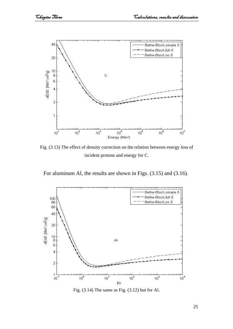
For aluminum Al, the results are shown in Figs. (3.15) and (3.16).
Fig. (3.14) The same as Fig. (3.12) but for Al.
Chapter Three Calculations, results and discussion
26
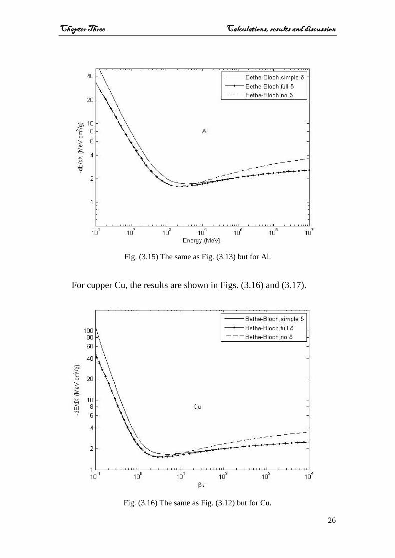
Fig. (3.15) The same as Fig. (3.13) but for Al.
For cupper Cu, the results are shown in Figs. (3.16) and (3.17).
Fig. (3.16) The same as Fig. (3.12) but for Cu.
Chapter Three Calculations, results and discussion
27
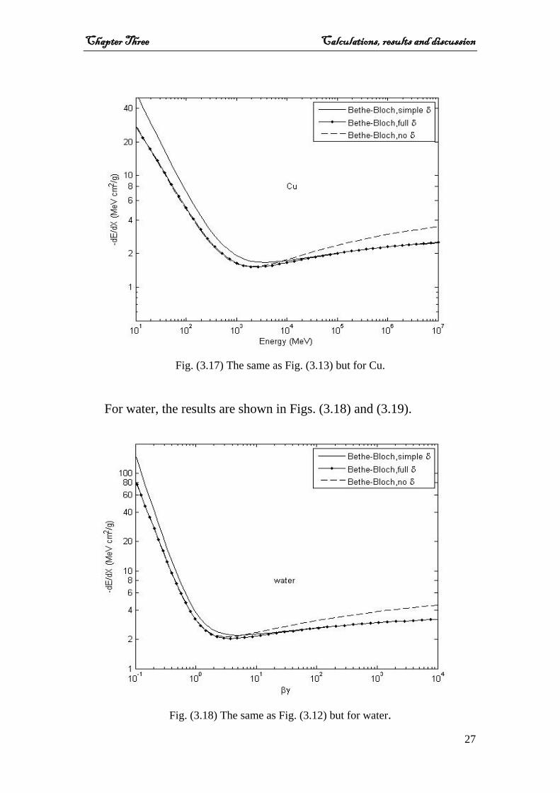
Fig. (3.17) The same as Fig. (3.13) but for Cu.
For water, the results are shown in Figs. (3.18) and (3.19).
Fig. (3.18) The same as Fig. (3.12) but for water.
Chapter Three Calculations, results and discussion
28
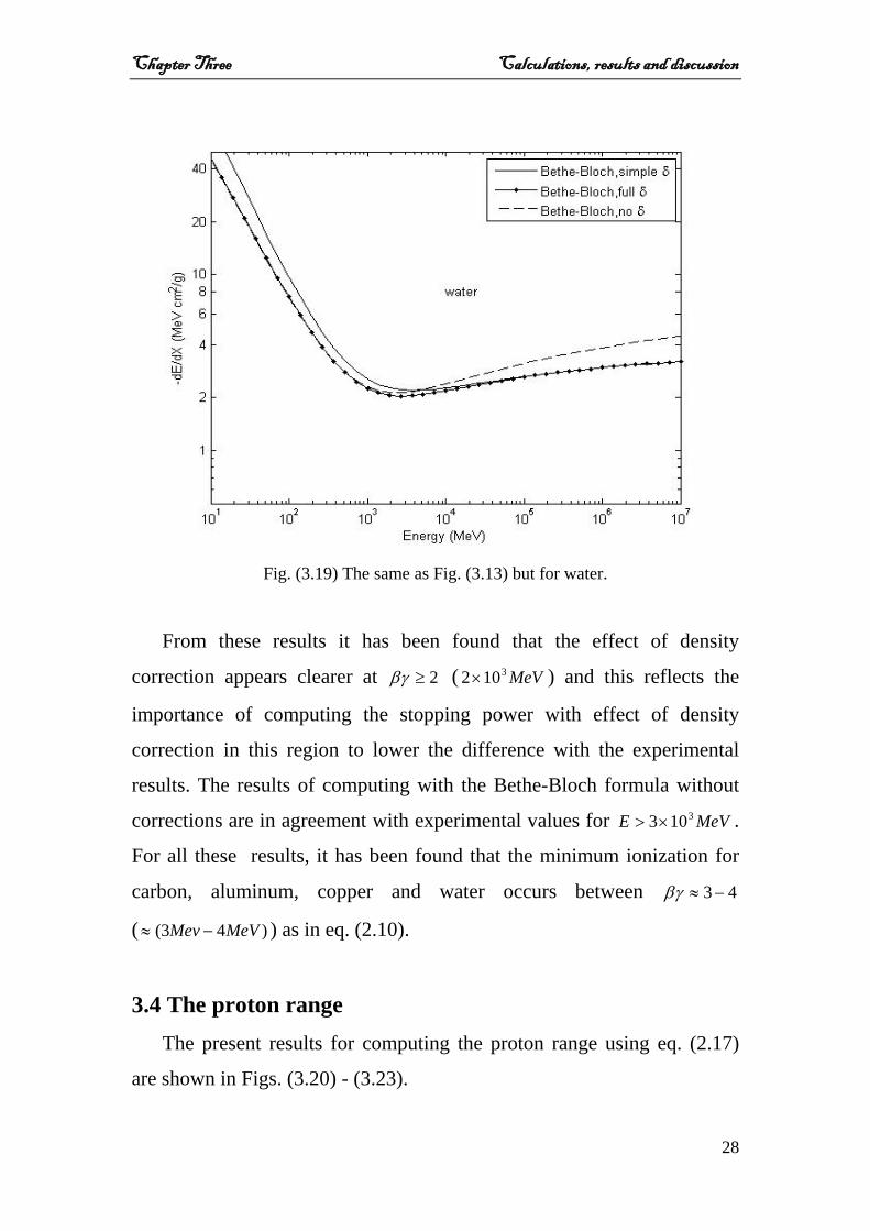
Fig. (3.19) The same as Fig. (3.13) but for water.
From these results it has been found that the effect of density
correction appears clearer at 2≥βγ ( MeV3102× ) and this reflects the
importance of computing the stopping power with effect of density
correction in this region to lower the difference with the experimental
results. The results of computing with the Bethe-Bloch formula without
corrections are in agreement with experimental values for MeVE 3103×> .
For all these results, it has been found that the minimum ionization for
carbon, aluminum, copper and water occurs between 43−≈βγ
( )43( MeVMev −≈ ) as in eq. (2.10).
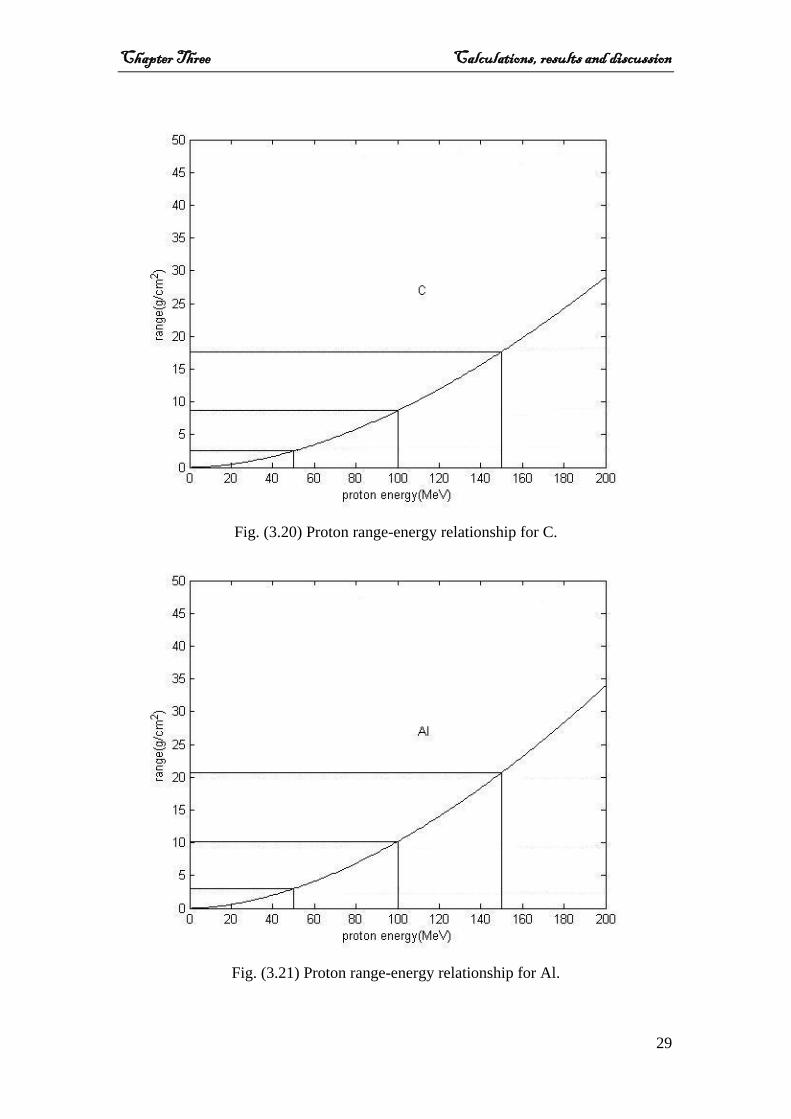
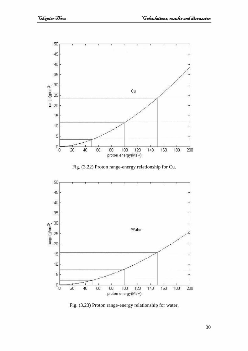
3.4 The proton range
The present results for computing the proton range using eq. (2.17)
are shown in Figs. (3.20) - (3.23).
Chapter Three Calculations, results and discussion
29
Fig. (3.20) Proton range-energy relationship for C.
Fig. (3.21) Proton range-energy relationship for Al.
Chapter Three Calculations, results and discussion
30
Fig. (3.22) Proton range-energy relationship for Cu.
Fig. (3.23) Proton range-energy relationship for water.
Chapter Three Calculations, results and discussion
31
The range of the proton increases when the incident proton energy
increases. The horizontal lines represent the range for 50 MeV, 100 MeV,
150 MeV proton energies.
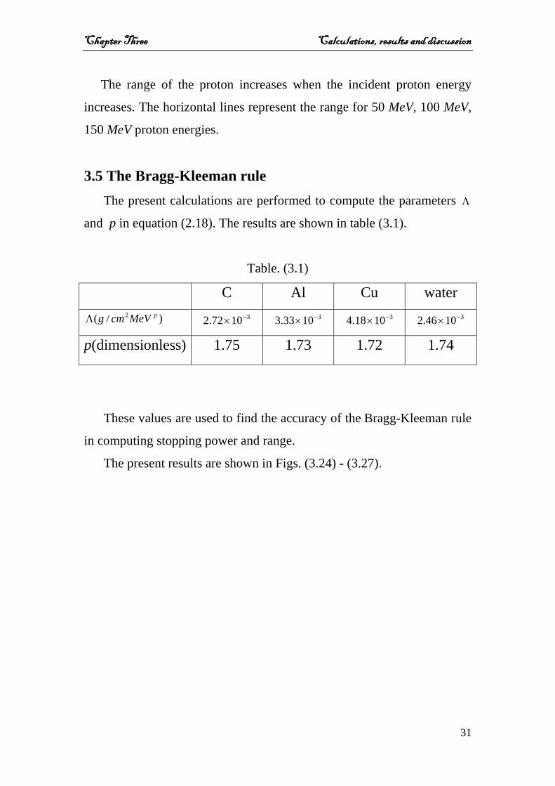
3.5 The Bragg-Kleeman rule The present calculations are performed to compute the parameters Λ
and p in equation (2.18). The results are shown in table (3.1).
Table. (3.1)
C Al Cu water
)/( 2 pMeVcmgΛ 31072.2 −× 31033.3 −× 31018.4 −× 31046.2 −×
p(dimensionless) 1.75 1.73 1.72 1.74
These values are used to find the accuracy of the Bragg-Kleeman rule
in computing stopping power and range.
The present results are shown in Figs. (3.24) - (3.27).
Chapter Three Calculations, results and discussion
32
Fig. (3.24) The relationship between energy loss and energy for C calculated using the
Bragg-Kleeman rule and using the Bethe-Bloch formula.
Fig. (3.25) The same as Fig. (3.24) but for Al.
Chapter Three Calculations, results and discussion
33
Fig. (3.26) The same as Fig. (3.24) but for Cu.
Fig. (3.27) The same as Fig. (3.24) but for water.

Chapter Three Calculations, results and discussion
34
From these results it has been found that the values of the stopping
power calculated using the Bragg-Kleeman rule are in agreement with the
stopping power calculated using the Bethe-Bloch formula for
MeVE 200≤ .
The comparison of the computed ranges for the two cases are shown
Figs. (3.28)-(3.31).
Fig. (3.28) The range calculated by integrating the Bethe-Bloch formula and by the
Bragg-Kleeman rule as a function of energy for C.
Chapter Three Calculations, results and discussion
35
Fig. (3.29) The same as Fig. (3.28) but for Al.
Fig. (3.30) The same as Fig. (3.28) but for Cu.
Chapter Three Calculations, results and discussion
36
Fig. (3.31) The same as Fig. (3.28) but for water.
From these results it has been found that the proton range calculated
by the Bragg-Kleeman rule is in agreement with the range calculated by
the Bethe-Bloch formula for proton energies MeVE 400≤ .
The stopping power-range relationships computed by the Bethe-Bloch
formula and by the Bragg-Kleeman rule are shown in Figs. (3.32)-(3.35).
Chapter Three Calculations, results and discussion
37
Fig. (3.32) The stopping power-range relationship computed by the Bethe-Bloch
formula and the Bragg-Kleeman rule for C.
Fig. (3.33) The same as Fig. (3.32) but for Al.
Chapter Three Calculations, results and discussion
38
Fig. (3.34) The same as Fig. (3.32) but for Cu.
Fig. (3.35) The same as Fig. (3.32) but for water.
Chapter Three Calculations, results and discussion
39
It has been found the results for the relationship between the stopping
power and range calculated by the Bethe-Bloch formula and by the
Bragg-Kleeman rule are in agreement.
3.5 Energy deposition For energy deposition, the results of comparison between the
computed results of the Bethe-Bloch formula and the Bragg-Kleeman
rule are shown in Figs. (3.36)-(3.39).
Fig. (3.36) The range computed by integrating the Bethe-Bloch formula and by the
Bragg-Kleeman rule as a function of energy for C.
Chapter Three Calculations, results and discussion
40
Fig. (3.37) The same as Fig. (3.36) but for Al.
Fig. (3.38) The same as Fig. (3.36) but for Cu.
Chapter Three Calculations, results and discussion
41
Fig. (3.39) The same as Fig. (3.36) but for water.
From these results it has been found the energy of the proton
decreases sharply at the end of its path and the results for the energy
deposition calculated using the Bethe-Bloch formula and the Bragg-
Kleeman rule are in agreement.
The comparisons between the linear energy transfer values (the dose
averaged LET) calculated using the Bethe-Bloch formula and the Bragg-
Kleeman rule are shown in Figs. (3.40)-(3.43).

Chapter Three Calculations, results and discussion
42
Fig. (3.40) Dose averaged LET-range relationship computed using the Bethe-Bloch
formula and the Bragg-Kleeman rule for C.
Fig. (3.41) The same as Fig, (3.40) but for Al.
Chapter Three Calculations, results and discussion
43
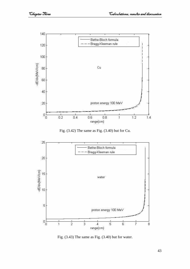
Fig. (3.42) The same as Fig. (3.40) but for Cu.
Fig. (3.43) The same as Fig. (3.40) but for water.
Chapter Three Calculations, results and discussion
44
From these figures it has been found that the stopping power of
protons is approximately constant except at the end of its path where it
becomes very high because the proton looses all its kinetic energy in this
region. The results of the dose averaged LET range for protons calculated
by integrating the Bethe-Bloch formula and the Bragg-Kleeman rule are
in agreement.

Chapter Four
Conclusions and
recommendations

Chapter four Conclusion and recommendations
45
4.1 Conclusions From the present work, it can be concluded that:
1.The stopping power computed using the Bethe-Bolch formula without
corrections is in agreement with experimental results for 2≤βγ
( MeVE 3102×≤ ).
2. The results of computing the stopping power using the Bethe-Bolch
formula with density correction is in agreement with experimental results
for 210≤βγ ( MeVE 510≤ ), assuming that this formula remains correct at
these energies.
3. For MeVE 510≥ , it is concluded from the present results that the
density correction and the effect of maximum energy are important to
lower the differences between theoretical and experimental results.
4. The results of computing the stopping power by the Bragg-Kleeman
rule are in agreement with experimental results for MeVE 200≤ .
5. The values of calculation of the range by the Bragg-Kleeman rule are
in agreement with experimental results for MeVE 400≤ .
6. Proton looses a great percentage of its initial energy at the end of its
path in the medium and the stopping power becomes very high.
4.2 Recommendations
This work can be extended to include other aspects as follows:
1. Calculating the stopping power and range for protons with
maximum energy effect and density correction for other elements
and compounds [10].
2. Using the maximum energy and density correction for light
charged particles (electron, positron, etc ) to study their effects on
the previously calculated results for these particles [10].
Chapter four Conclusion and recommendations
46
3. Studying the effects of the maximum energy and density
correction using heavy charged particles (deuterons and alpha
particles) on different elements.

References
References
47
References:
1. L. Foschini, "The fingers of the physics", Annales de la Foundation
Louis de Broglie, Vol. 25, No. 1, pp. 67-79, (2000).
2. P. Wijesinghe, "Energy deposition study of low-energy cosmic
radiation at sea level", Ph.D. Thesis, The College of Arts and
Sciences, Georgia State University, (2007).
3. A. Z. Jones, C. D. Bloch, E. R. Hall, R. Hashemian, S. B. Klein, B.
von Przewoski, K. M. Murray and C. C. Foster, "Comparison of
Indiana University cyclotron factory Faraday cup proton dosimetry
with radiochromic films, a calorimeter and calibrated ion chamber'',
IEEE, Indiana University Cyclotron Facility, Bloomington, IN
47408, USA, (1998).
4. J. T. Lyman, C. M. Awschalom, P. Berardo, H. Bicchsel, G. T. Y.
Chen, J. Dicello, P. Fessenden, M. Goitein, G. Lam, J. C. McDonald,
A. Ft. Smith, R. T. Haken, L. Verhey, S. Zink, "Protocol for heavy
charged-particle therapy beam dosimetry", The American
Association of Physicists in Medicine, AAPM report No. 16, (1986).
5. M. J. Butson, P K.N. Yu, T. Cheung, P. Metcalfe, " Radiochromic
film for medical radiation dosimetry ", Materials Science and
Engineering R, Vol. 41, pp. 61-120, (2003).
6. M. Noll, W. Schöner, N. Vana1, M. Fugger, E. Egger,
"Measurements of the Linear Energy Transfer LET in a proton of 62
MeV using the High Temperature Ratio HTR-Method", in
Microdosimetry. An Interdisciplinary Approach. D.T. Goodhead,
edited by P. O’Neill, H.G. Menzel (Eds.), The Royal Society of
Cambridge, pp. 274-277, (1997).
References
48
7. J. J. Wilkens," Evaluation of Radiobiological Effects in Intensity
Modulated Proton Therapy: New Strategies for Inverse Treatment
Planning", Ph.D. Thesis, Ruperto-Carola University of Heidelberg,
Germany, (2004).
8. R. W. Peelle, "Rapid computation of specific energy losses for
energetic charged particles", OAK Ridge National Laboratory,
Union Carbide Corporation, ONRL-TM-977, COPY NO. -71, April
29, (1965).
9. W. R. Nelson, "Accelerator Beam Dosimetry", SLAC-PUB-1803,
(1976).
10. D. Groom, "Energy loss in matter by heavy particles", Particle Data
Group Notes, PDG-93-06, (1993).
11. J. Wasjenaar, "Charged particle interactions", Joint Program in
Nuclear Medicine (JPNM Physics), Harvard Medical School,
Department of Radiology, (1994).
12. H. Tai, H. Bichsel, J. W. Wilson, F. F. Badavi, "Comparison of
stopping power and range databases for radiation transport study",
NASA Technical paper 3644, (1997).
13. B. VanKuik, C. Gardner, S. Bellavia, A. Rusek, K. Brown, "NSRL
energy loss calculator", Collider-Acceletor Department, Brookhaven
National Laboratory, Report No. C-A/AP/#251, Upton, NY 11973,
August (2006).
14. J. F. Ziegler, "The Stopping of Energetic Light Ions in Elemental
Matter", Physical Review A, Vol. 85, pp. 1249-1272, (1999).
15. J. C. Armitage, M. S. Dixit, J. Dubeau, H. Mes, F. G. Oakham,
"Charged Particle Measurements", CRC Press LLC, (2000).
16. P. T. Leung, "Bethe stopping-power theory for heavy-target atoms",
Physical Review A, Vol. 60, No. 3, pp. 2562-2564, (1999).

References
49
17. V. V. Gann, "Investigation of the energy deposition profile in
NaCl", Nuclear Physics Investigations, Vol. 42, No. 1, pp. 197-199,
(2004).
18. P. Sigmund, A. Schinner, " Shell correction in stopping theory",
Nuclear Instruments and Methods in Physics Research Section B,
Vol. 243, Issue 2, pp. 457-460, February, (2006).
19. M. F. Zaki, A. Abdel-Naby, A. A. Morsy, "Single-sheet
identification method of heavy charged particles using solid state
nuclear track detectors", PRAMANA-journal of physics, Indian
Academy of Sciences, Vol. 69, No. 2, pp. 191-198, (2007).
20. Ö. Kabadayi, "Range of medium and high energy protons and alpha
particles in NaI scintillator", Acta Physica Polonica B, Vol. 37, No.
6, pp. 1847-1854, (2006).
21. F. Maas, "Interaction of particles with matter and main types of
detectors I", General FANTOM Study Week on Experimental
Techniques and Data Handling, Paris, France, IPN Orsay, 29 May - 2
June, (2006).
22. R. L. Murray, "Nuclear energy", Butterworth Heinemann, Fifth
Edition, (2000).
23. W. N. Cottingham, D. A. Greenwood, "An introduction to nuclear
physics", Cambridge University Press, Second Edition, (2004).
24. B. R. Martin, "Nuclear and particle physics", John Wiley & Sons,
Ltd, (2006).
25. R. Lozeva, "A new developed calorimeter telescope for
identification of relativistic heavy ion reaction channels", Ph.D.
Thesis, University of Sofia, "St. Kliment Ohridski", Faculty of
Physics, (2005) .

الخالصة
إن عملية حساب قيم قدرة اإليقاف ومدى االختراق للبروتون تتم بطريقتين :
الطريقة األولى باستخدام معادلة بيتا-بلوخ و الطريقة الثانية باستخدام معادلة براك-
كليمان و االختالف بين النتائج النظرية و النتائج التجريبية يتطلب دراسة
التصحيحات لمعادلة بيتا-بلوخ المتمثلة بالطاقة القصوى و تصحيح الكثافة و مقارنة
النتائج مع النتائج التجريبية. بدراسة تلك المعادالت وجدنا أن نتائج حساب معادلة
بيتا-بلوخ بدون تصحيحات الطاقة القصوى و تصحيح الكثافة تكون متوافقة مع
βγ(MeVE≥2النتائج التجريبية للطاقات ( βγ( MeVE≥210 و (≥×3102 510≤
مع التصحيحات. إن تأثير الطاقة القصوى و تصحيح الكثافة يساهمان في تقليل
βγ (MeVE≤210االختالف مع النتائج التجريبية للطاقات ( 510≥ .
إن قيم قدرة اإليقاف المحسوبة باستخدام معادلة براك-كليمان تكون متوافقة مع
MeVEالنتائج التجريبية للطاقات وقيم مدى االختراق المحسوبة باستخدام ≥200
معادلة براك-كليمان متوافقة مع النتائج المحسوبة باستخدام معادلة بيتا-بلوخ للطاقات
MeVE 400≤ .
أظهرت النتائج أن معدل الخسارة في الطاقة للبروتون عند الطاقات العالية يكون
صغيراً والعكس صحيح حيث إن معدل الخسارة للبروتون عند الطاقات الواطئة
يكون عالياً .
تؤكد النتائج الحالية إن البروتون يفقد نسبة كبيرة من طاقته في نهاية مساره في
المادة .
يقافاإلدراسة قدرة ات للبروتونمدىو ال
رسالة
الحصول علىمقدمة إلى كلية العلوم جامعة النهرين كجزء من متطلبات في الفيزياء علوم الماجستيردرجة
من قبلمصطفى عبد المحسن عبد العالي
) ۲۰۰٥س بكالوريو(
ه۱٤۳۰ م۲۰۰۹
شوال تشرين األول
جمهورية العراق والبحث العلمي ي وزارة التعليم العال
جامعة النهرين كلية العلوم