Study of fluid flow within the hearing organ

Xavier Meyer1, Elisabeth Delevoye2 and Bastien Chopard1

1Department of Computer Science, University of Geneva, Switzerland.2CEA-Grenoble DRT/DSIS/SCSE, France.

Abstract

Georg Von Bekesy was awarded a nobel price in 1961 for his pi-oneering work on the cochlea function in the mammalian hearing or-gan [2]. He postulated that the placement of sensory cells in the cochleacorresponds to a specific frequency of sound. This theory, known astonotopy, is the ground of our understanding on this complex organ.With the advance of technologies, this knowledge broaden continuouslyand seems to confirm Bekesy initial observations. However, a mysterystill lies in the center of this organ: how does its microscopic tissuesexactly act together to decode the sounds that we perceive ?

One of these tissues, the Reissner membrane, forms a double celllayer elastic barrier separating two fundamental ducts of this organ.Yet, until recently [16], this membrane, was not considered in themodelling of the inner ear due to its smallness. Nowadays, objectsof this size are at the reach of the medical imagining and measuringexpertise [18, 4, 16]. Newly available observations coupled with theincreasing availability of computational resources should enable mod-ellers to consider the impact of these microscopic tissues in the innerear mechanism.

In this report, we explore the potential fluid-structure interactionshappening in the inner ear, more particularly on the Reissner mem-brane. This study aims at answering two separate questions :

• Can nowadays computational fluid dynamics solvers simulate in-teraction with inner ear microscopic tissues ?

• Has the Reissner membrane function on the auditory system beenoverlooked ?

This report is organized as follow. Starting with a brief state of theart, the first section introduces the required notions to understand theexperiments. The anatomy and the function of the cochlea are sum-marized and the main concepts of the computational fluid dynamicsmethod used are defined. The next two sections presents the settingof the simulations and their results : the first focuses on the vestibu-lar duct and the Reissner membrane while the second focuses on thecochlear duct and the organ of Corti. We conclude in the final sectionby discussing the numerical experiments results.

1

arX

iv:1

709.

0679

2v1

[ph

ysic

s.bi

o-ph

] 2

0 Se

p 20

17

1 Introduction1.1 State of the artNowadays, more than 60’000 hearing impaired persons benefits fromcochlear implants [25]. These devices design is strongly tied to ourunderstanding of the hearing organ. Its main component, the cochlea,processes acoustic signals by the mean of a complex mechanism. Sincethe early work of Georg Von Bekesy [1, 2], research on the mammalcochlea has been the focus of many scientists [21, 17]. Yet, this mech-anism is not fully understood.

In order to fill this knowledge gap, a large amount of cochlear mod-els have been developed through the years [15]. Given the complexity ofthe hearing organ, these models focus on a set of selected phenomenon: cochlear micro- or macro-mechanics with or without fluid coupling.Macro-mechanics models represent roughly the cochlea as a box withthe vestibular and tympanic ducts separated by the vibrating basilarmembrane [5, 14, 27]. Micro-mechanics models focus on reproducingmore accurately the organ of Corti [3, 7, 19]. While all these modelsvary in the methods used and the size of phenomena simulated, theyall start with the same assumption that the Reissner membrane doesnot play any major role in the mechanics of the cochlea [15]. However,this membrane, that separates two fundamental ducts of the cochlea,has been shown to propagate travelling waves in a comparable fashionas the widely considered basilar membrane [16].

To our knowledge, computational fluid dynamics (CFD) has onlybeen used in one model [8]. This model presented an analysis of themacro-mechanics of the cochlea using immersed boundary conditions: a method simulating solid structure immersed in fluids. Our work isbased on a similar simulation method but differs strongly in its aim.Our focus is the under-considered deformation of the Reissner mem-brane and its induced fluid displacement. We postulate that such fluidmovements could impact the microscopic elements of Corti’s organ andtherefore play a key role in the hearing mechanism. In order to tacklethis challenge of representing both the inner ear micro- and macro-mechanics in the same simulation setting, we use a highly-parallel CFDcode, Palabos1.

1.2 Cochlea : the hearing organ1.2.1 AnatomyThe inner ear is composed of two major organ linked by the vestibule: the vestibular system and the cochlea (Fig. 1B). The main functionof the first one is the sense of balance, while the second contains theprimary auditory organ of the inner ear [24].

The cochlea whose name comes from the ancient greek kohlias,meaning spiral or snail shell, is structured as a spiral-shaped cavity.This cavity is considered to start from the base in the middle of the

1http://www.palabos.org/

2

Vestibularsystem

Cochlea

A) B)

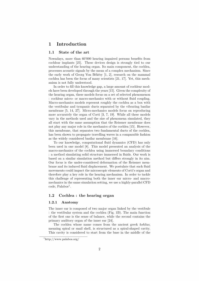
Figure 1: Figure A) shows the chain of transmission of sound with the tympanicmembrane (red), the ossicles (green) and the inner ear (blue). Figure B) shows theinner ear with its two main components : the vestibular system and the cochlea.Figures are adapted from [9].

vestibule and continues until it reaches its apex, the helicotrema. Inhumans, this canal forms in average 2.5 turns over 35mm and is sepa-rated by a thin spiral shelf of bone, the osseous spiral lamina (Fig. 2A).

13

2

56

4A) B)

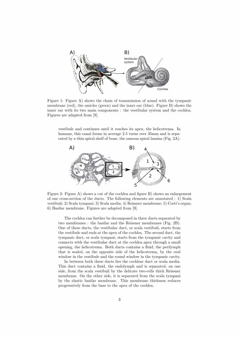
Figure 2: Figure A) shows a cut of the cochlea and figure B) shows an enlargementof one cross-section of the ducts. The following elements are annotated : 1) Scalavestibuli; 2) Scala tympani; 3) Scala media; 4) Reissner membrane; 5) Corti’s organ;6) Basilar membrane. Figures are adapted from [9].

The cochlea can further be decomposed in three ducts separated bytwo membranes : the basilar and the Reissner membranes (Fig. 2B).One of these ducts, the vestibular duct, or scala vestibuli, starts fromthe vestibule and ends at the apex of the cochlea. The second duct, thetympanic duct, or scala tympani, starts from the tympanic cavity andconnects with the vestibular duct at the cochlea apex through a smallopening, the helicotrema. Both ducts contains a fluid, the perilymphthat is sealed, on the opposite side of the helicotrema, by the ovalwindow in the vestibule and the round window in the tympanic cavity.

In between both these ducts lies the cochlear duct or scala media.This duct contains a fluid, the endolymph and is separated, on oneside, from the scala vestibuli by the delicate two-cells thick Reissnermembrane. On the other side, it is separated from the scala tympaniby the elastic basilar membrane. This membrane thickness reducesprogressively from the base to the apex of the cochlea.

3

Figure 3: Organ of Corti (adapted from [9]).

Inside the scala media, on top of the basilar membrane rests thesmall yet important organ of Corti (Fig. 3). This complex organ con-tains the fundamental element that translates the sound vibrations intonervous signals : the inner ear hair cells. These cells stand in a smallcanal, closed on one side by the basilar membrane and on the otherside by the tectorial membrane.

1.2.2 The hearing mechanismAcoustic signals are conveyed in the inner ear by a vibratory pattern.Acoustic waves reach the external auditory canal, the tympanic mem-brane, and transmit vibrations through the ossicles, a complex of smallbones (malleus, incus, stapes). These bones amplify the vibratory sig-nal before applying it to the oval windows (Fig. 1A2). In turn, thismembranous window transmits the vibrations to the vestibule and tothe inner ear fluid. These vibrations in the fluids are considered tocreate a travelling wave on the basilar membrane. The wave evolvefrom the base toward the apex for a length inversely proportional toits frequency. Therefore the placement, along the cochlea, of inner earhair cells defines the sound frequencies that activate them.

This theory, more known as tonotopy, was proposed by Georg VonBekesy [1, 2] and is based on his observations of the basilar mem-brane vibratory response when excited by sounds. This explanation ofthe hearing mechanism grossly simplify the reality by hiding complexmicro-mechanical phenomenon occurring in the organ of Corti. More-over, it doesn’t account of the role of the Reissner membrane. Morecomplex hypothesis are still explored in order to explain the impact ofthe Reissner membrane [16] or the role of the cochlea active mechanismthat produce otoacoustic emissions [11].

2The tympanic membrane or eardrum is represented in red and the ossicles in green.

4

1.3 Computational fluid simulations1.3.1 Palabos, an open source highly parallel solverIn order to simulate the complex fluid-solid phenomenons occurringin the inner ear, we used the lattice Boltzmann method (LBM). Thismethod is a modern approach in Computational Fluid Dynamics. It isoften used to solve the incompressible, time-dependent Navier-Stokesequations numerically. Its strength lies in the ability to easily repre-sent complex physical phenomena, ranging from multiphase flows tochemical interactions between the fluid and the surroundings. Themethod finds its origin in a molecular description of a fluid and candirectly incorporate physical terms stemming from a knowledge of theinteraction between molecules.

Unlike traditional CFD methods, LBM models the fluid consistingof fictive particles, and such particles perform consecutive propagationand collision processes over a discrete lattice mesh. Due to its par-ticulate nature and local dynamics, LBM has several advantages overother conventional CFD methods, especially in dealing with complexboundaries, incorporating microscopic interactions, and parallelizationof the algorithm3. For that matter, we chose ot use the open-sourcesoftware Palabos4. This software is a massively-parallel Lattice Boltz-mann implementation that have been used in numerous applicationssuch as the simulation of blood cells deposition in aneurysms [26] orpermeability change of porous medium [10].

In order to simulate membranes, Palabos maintainers developed anelastic shell model. In this model, the fluid domain is bounded by time-independent boundaries (rigid walls) and time-dependent boundaries(membranes). During the simulation, the fluid-structure interaction istaken in account at these boundary such as to apply internal forceson the elastic wall. The time dynamics of the wall is then solved andthe fluid domain is recomputed to adapt to these changes. This modelimplement all these steps as to be second-order accurate and offers agood scaling for parallel execution.

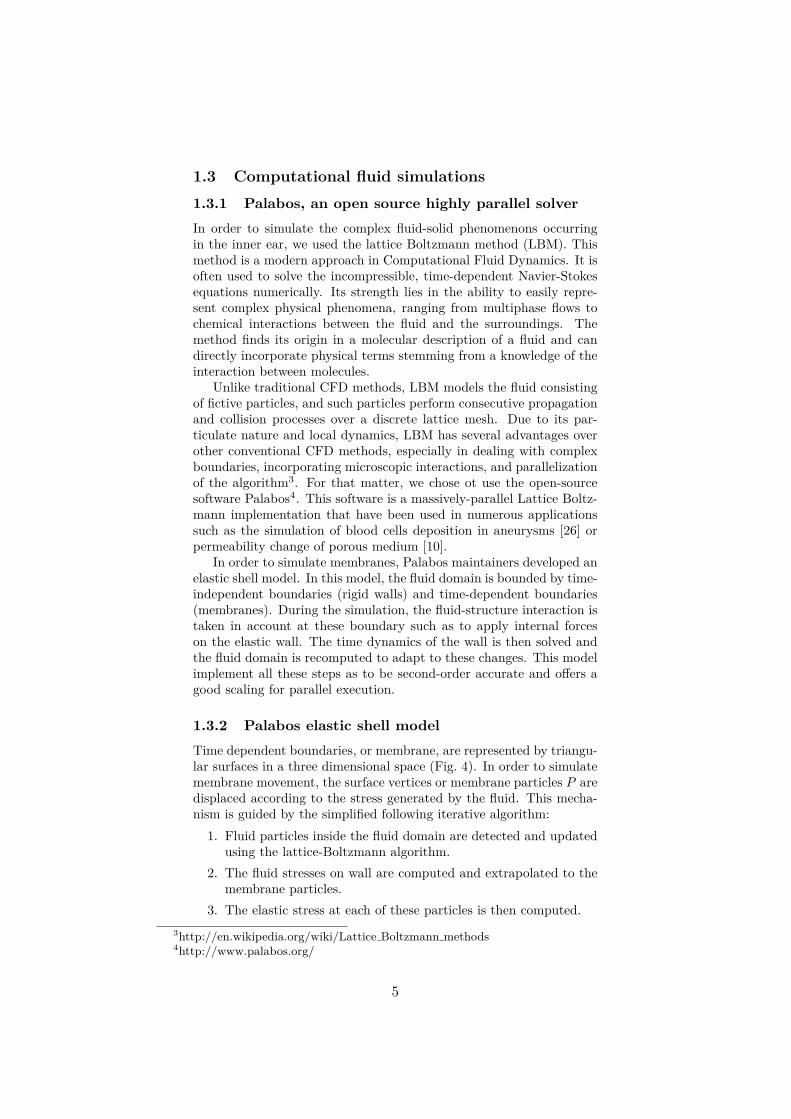
1.3.2 Palabos elastic shell modelTime dependent boundaries, or membrane, are represented by triangu-lar surfaces in a three dimensional space (Fig. 4). In order to simulatemembrane movement, the surface vertices or membrane particles P aredisplaced according to the stress generated by the fluid. This mecha-nism is guided by the simplified following iterative algorithm:

1. Fluid particles inside the fluid domain are detected and updatedusing the lattice-Boltzmann algorithm.

2. The fluid stresses on wall are computed and extrapolated to themembrane particles.

3. The elastic stress at each of these particles is then computed.3http://en.wikipedia.org/wiki/Lattice Boltzmann methods4http://www.palabos.org/

5

4. Membrane particles advance according to Newton’s law.5. The off-lattice boundary condition is reconstructed according to

the new membrane position.

Figure 4: Representation of a time-dependent boundary and the three forces actingon it : stretching, shearing and bending.

The elasticity of the membrane is characterized by a complex modelformed of stretching, bending and shearing forces (Fig. 4). The firstforce is modelled by considering the edges between vertex as springwith linear attractive forces. The second is insured by preserving theon-membrane angles. The latter is defined as the preservation of thetriangular surfaces area.

At each iteration, these elastic forces are computed and used torepresent the acceleration of each membrane particles. The elasticpotential of a particle U is represented by multiple potential in orderto represent as realistically as possible the three dimensions.

The stretch potential exists between a particle P and each of itsneighbours. This potential is given by

Ustretch = 0.5 · kstretch · (l − lEQ)2

where l stand for the distance between the particles at this iterationand lEQ their distance at equilibrium.

The bending potential represent the angular elasticity of the mem-brane. For a given membrane particle, each pair of adjacent triangularsurface generate a bending potential given by

Ubend = 0.5 · kbend · (α− αEQ)2 · lw

where α stands for the angle between both triangular surfaces, αEQ

the equilibrium angle, l represents the length of the shared edge. Thentile span w between both triangular surface is computed as w = h

6 withh being the summed height of the triangular surfaces.

The shear potential represent the elasticity of an area of membraneand exists for each triangular surface where the particle stand as avertex.

Ushear = 0.5 · kshear · (A−AEQ)2

6

where A represent the area of triangular surface and AEQ the area atequilibrium.

These three potentials are then summed in order to define the totalelastic potential of a given particle

U = Ustretch + Ushear + Ubend

and from this total potential, the force FU on a particle P is numeri-cally derived over all three dimensions X = (x1, x2, x3)

FU = dU

dX= U(x+ ε) − U(x− ε)

2 · ε

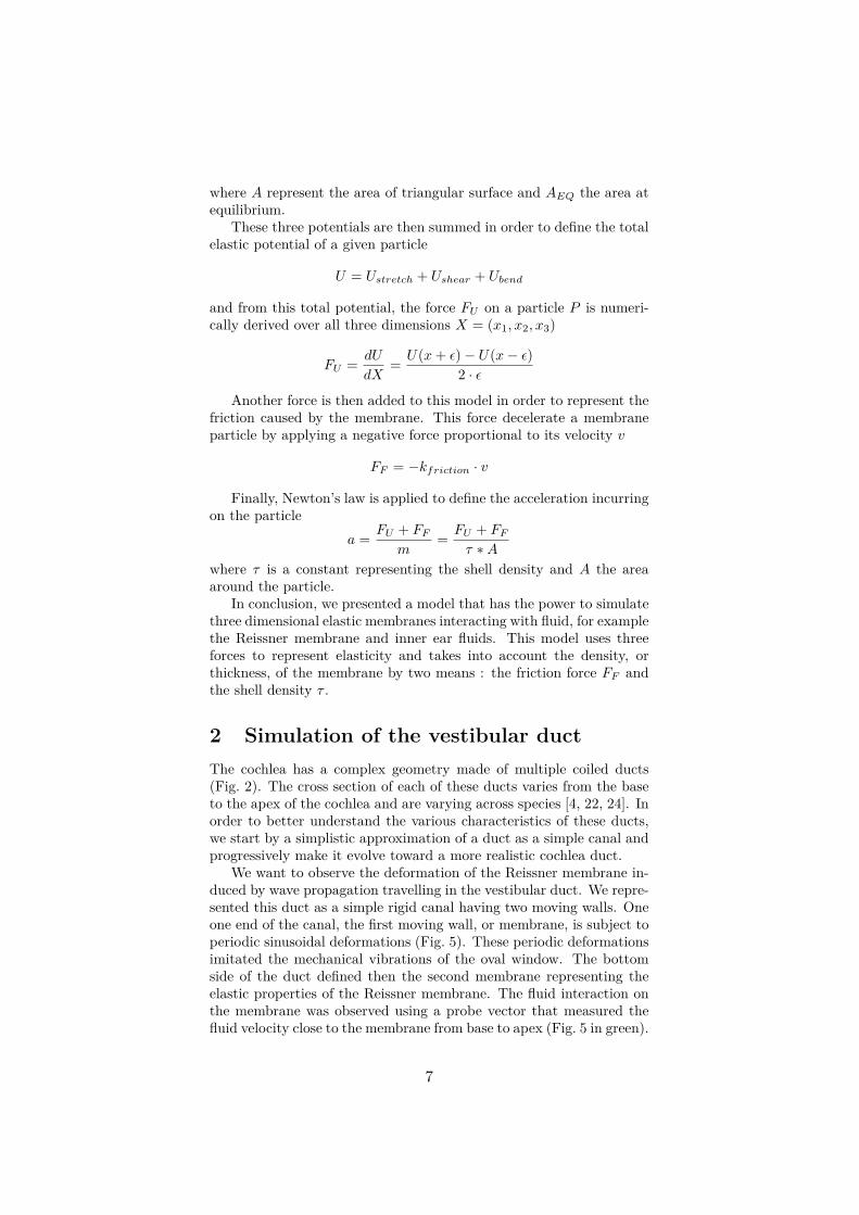
Another force is then added to this model in order to represent thefriction caused by the membrane. This force decelerate a membraneparticle by applying a negative force proportional to its velocity v

FF = −kfriction · v

Finally, Newton’s law is applied to define the acceleration incurringon the particle

a = FU + FF

m= FU + FF

τ ∗Awhere τ is a constant representing the shell density and A the areaaround the particle.

In conclusion, we presented a model that has the power to simulatethree dimensional elastic membranes interacting with fluid, for examplethe Reissner membrane and inner ear fluids. This model uses threeforces to represent elasticity and takes into account the density, orthickness, of the membrane by two means : the friction force FF andthe shell density τ .

2 Simulation of the vestibular ductThe cochlea has a complex geometry made of multiple coiled ducts(Fig. 2). The cross section of each of these ducts varies from the baseto the apex of the cochlea and are varying across species [4, 22, 24]. Inorder to better understand the various characteristics of these ducts,we start by a simplistic approximation of a duct as a simple canal andprogressively make it evolve toward a more realistic cochlea duct.

We want to observe the deformation of the Reissner membrane in-duced by wave propagation travelling in the vestibular duct. We repre-sented this duct as a simple rigid canal having two moving walls. Oneone end of the canal, the first moving wall, or membrane, is subject toperiodic sinusoidal deformations (Fig. 5). These periodic deformationsimitated the mechanical vibrations of the oval window. The bottomside of the duct defined then the second membrane representing theelastic properties of the Reissner membrane. The fluid interaction onthe membrane was observed using a probe vector that measured thefluid velocity close to the membrane from base to apex (Fig. 5 in green).

7

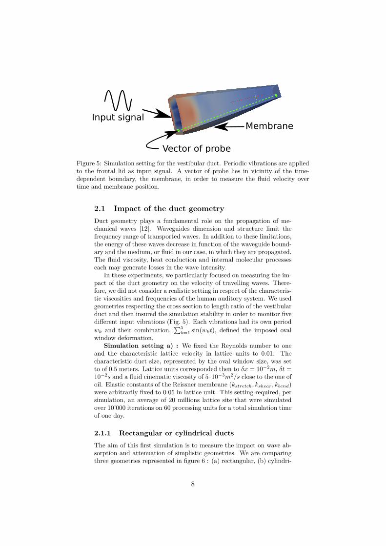
Input signalMembrane

Vector of probe

Figure 5: Simulation setting for the vestibular duct. Periodic vibrations are appliedto the frontal lid as input signal. A vector of probe lies in vicinity of the time-dependent boundary, the membrane, in order to measure the fluid velocity overtime and membrane position.

2.1 Impact of the duct geometryDuct geometry plays a fundamental role on the propagation of me-chanical waves [12]. Waveguides dimension and structure limit thefrequency range of transported waves. In addition to these limitations,the energy of these waves decrease in function of the waveguide bound-ary and the medium, or fluid in our case, in which they are propagated.The fluid viscosity, heat conduction and internal molecular processeseach may generate losses in the wave intensity.

In these experiments, we particularly focused on measuring the im-pact of the duct geometry on the velocity of travelling waves. There-fore, we did not consider a realistic setting in respect of the characteris-tic viscosities and frequencies of the human auditory system. We usedgeometries respecting the cross section to length ratio of the vestibularduct and then insured the simulation stability in order to monitor fivedifferent input vibrations (Fig. 5). Each vibrations had its own periodwk and their combination,

∑5k=1 sin(wkt), defined the imposed oval

window deformation.Simulation setting a) : We fixed the Reynolds number to one

and the characteristic lattice velocity in lattice units to 0.01. Thecharacteristic duct size, represented by the oval window size, was setto of 0.5 meters. Lattice units corresponded then to δx = 10−2m, δt =10−2s and a fluid cinematic viscosity of 5 ·10−3m2/s close to the one ofoil. Elastic constants of the Reissner membrane (kstretch, kshear, kbend)were arbitrarily fixed to 0.05 in lattice unit. This setting required, persimulation, an average of 20 millions lattice site that were simulatedover 10’000 iterations on 60 processing units for a total simulation timeof one day.

2.1.1 Rectangular or cylindrical ductsThe aim of this first simulation is to measure the impact on wave ab-sorption and attenuation of simplistic geometries. We are comparingthree geometries represented in figure 6 : (a) rectangular, (b) cylindri-

8

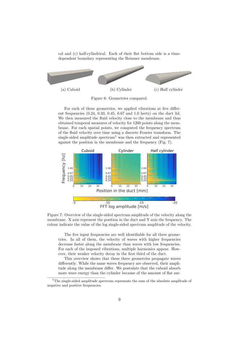
cal and (c) half-cylindrical. Each of their flat bottom side is a time-dependent boundary representing the Reissner membrane.

(a) Cuboid (b) Cylinder (c) Half cylinder

Figure 6: Geometries compared.

For each of these geometries, we applied vibrations at five differ-ent frequencies (0.24, 0.33, 0.45, 0.67 and 1.0 hertz) on the duct lid.We then measured the fluid velocity close to the membrane and thusobtained temporal measures of velocity for 1200 points along the mem-brane. For each spatial points, we computed the frequency spectrumof the fluid velocity over time using a discrete Fourier transform. Thesingle-sided amplitude spectrum5 was then extracted and representedagainst the position in the membrane and the frequency (Fig. 7).

Freq

uency

[hz]

0.240.330.450.67

1.00

0 10 20 30

Cuboid Cylinder Half cylinder

0.240.330.450.67

1.00

0.240.330.450.67

1.00

0 10 20 30 0 10 20 30

Position in the duct [mm]

-5 -10 -15 -20FFT log amplitude [m/s]

Figure 7: Overview of the single-sided spectrum amplitude of the velocity along themembrane. X axis represent the position in the duct and Y axis the frequency. Thecolour indicate the value of the log single-sided spectrum amplitude of the velocity.

The five input frequencies are well identifiable for all three geome-tries. In all of them, the velocity of waves with higher frequenciesdecrease faster along the membrane than waves with low frequencies.For each of the imposed vibrations, multiple harmonics appear. How-ever, their weaker velocity decay in the first third of the duct.

This overview shows that these three geometries propagate wavesdifferently. While the same waves frequency are observed, their ampli-tude along the membrane differ. We postulate that the cuboid absorbmore wave energy than the cylinder because of the amount of flat sur-

5The single-sided amplitude spectrum represents the sum of the absolute amplitude ofnegative and positive frequencies.

9

face that reflect waves. Inded such reflection may cause interferencesthat attenuate the wave energy.

Position in the duct [mm]

FFT log

am

plt

iud

e [

m/s

]

0 10 20 30

-4

-6

-8

-10

-12

-14

-16

-18

a) Signal at 0.24Hz

0 10 20 30-20

-15

-10

-5 CuboidCylinderHalf Cylinder

b) Signal at 0.66Hz

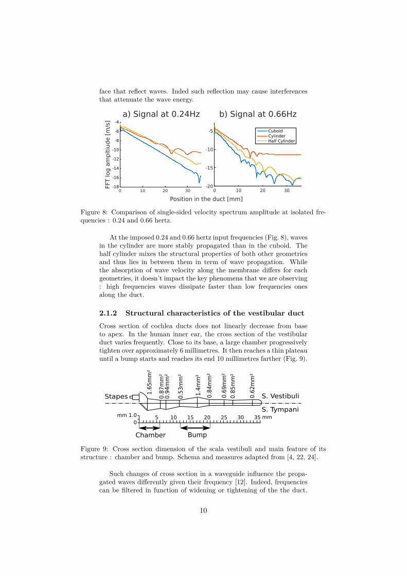
Figure 8: Comparison of single-sided velocity spectrum amplitude at isolated fre-quencies : 0.24 and 0.66 hertz.

At the imposed 0.24 and 0.66 hertz input frequencies (Fig. 8), wavesin the cylinder are more stably propagated than in the cuboid. Thehalf cylinder mixes the structural properties of both other geometriesand thus lies in between them in term of wave propagation. Whilethe absorption of wave velocity along the membrane differs for eachgeometries, it doesn’t impact the key phenomena that we are observing: high frequencies waves dissipate faster than low frequencies onesalong the duct.

2.1.2 Structural characteristics of the vestibular ductCross section of cochlea ducts does not linearly decrease from baseto apex. In the human inner ear, the cross section of the vestibularduct varies frequently. Close to its base, a large chamber progressivelytighten over approximately 6 millimetres. It then reaches a thin plateauuntil a bump starts and reaches its end 10 millimetres farther (Fig. 9).

1.6

5m

m²

0.8

7m

m²

0.9

4m

m²

0.5

3m

m²

1.4

mm

²

0.8

4m

m²

0.6

9m

m²

0.8

5m

m²

0.6

2m

m²

mm 1.00

5 10 15 20 25 30 mm

Stapes S. Vestibuli

S. Tympani35

Chamber Bump

Figure 9: Cross section dimension of the scala vestibuli and main feature of itsstructure : chamber and bump. Schema and measures adapted from [4, 22, 24].

Such changes of cross section in a waveguide influence the propa-gated waves differently given their frequency [12]. Indeed, frequenciescan be filtered in function of widening or tightening of the the duct.

10

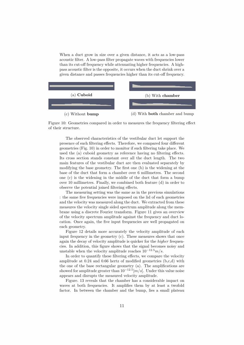
When a duct grow in size over a given distance, it acts as a low-passacoustic filter. A low-pass filter propagate waves with frequencies lowerthan its cut-off frequency while attenuating higher frequencies. A high-pass acoustic filter is the opposite, it occurs when the duct shrink over agiven distance and passes frequencies higher than its cut-off frequency.

(a) Cuboid (b) With chamber

(c) Without bump (d) With both chamber and bump

Figure 10: Geometries compared in order to measures the frequency filtering effectof their structure.

The observed characteristics of the vestibular duct let support thepresence of such filtering effects. Therefore, we compared four differentgeometries (Fig. 10) in order to monitor if such filtering take place. Weused the (a) cuboid geometry as reference having no filtering effects.Its cross section stands constant over all the duct length. The twomain features of the vestibular duct are then evaluated separately bymodifying the base geometry. The first one (b) is the widening at thebase of the duct that form a chamber over 6 millimetres. The secondone (c) is the widening in the middle of the duct that form a bumpover 10 millimetres. Finally, we combined both feature (d) in order toobserve the potential joined filtering effects.

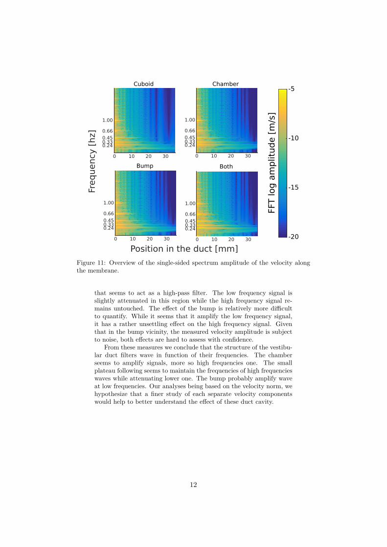
The measuring setting was the same as in the previous simulations: the same five frequencies were imposed on the lid of each geometriesand the velocity was measured along the duct. We extracted from thesemeasures the velocity single sided spectrum amplitude along the mem-brane using a discrete Fourier transform. Figure 11 gives an overviewof the velocity spectrum amplitude against the frequency and duct lo-cation. Once again, the five input frequencies are well propagated oneach geometry.

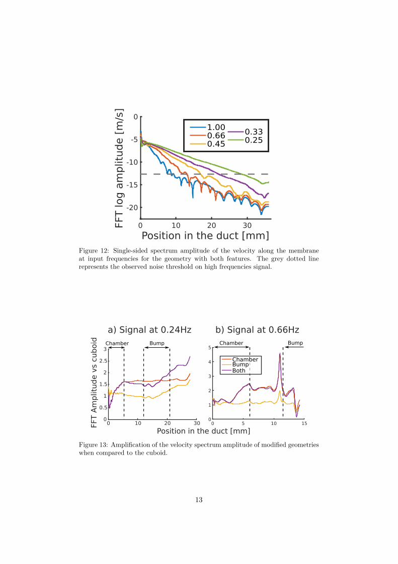
Figure 12 details more accurately the velocity amplitude of eachinput frequency in the geometry (c). These measures shows that onceagain the decay of velocity amplitude is quicker for the higher frequen-cies. In addition, this figure shows that the signal becomes noisy andunstable when the velocity amplitude reaches 10−12.5m/s.

In order to quantify these filtering effects, we compare the velocityamplitude at 0.24 and 0.66 hertz of modified geometries (b,c,d) withthe one of the base rectangular geometry (a). The amplifications areshowed for amplitude greater than 10−12.5[m/s]. Under this value noiseappears and disrupts the measured velocity amplitude.

Figure. 13 reveals that the chamber has a considerable impact onwaves at both frequencies. It amplifies them by at least a twofoldfactor. In between the chamber and the bump, lies a small plateau

11

Position in the duct [mm]

Freq

uency

[hz]

Bump

0 10 20 30

0.240.330.45

0.66

1.00

Cuboid

Both

Chamber

0 10 20 30

0.240.330.45

0.66

1.00

0 10 20 30

0.240.330.45

0.66

1.00

0 10 20 30

0.240.330.45

0.66

1.00

FFT log

am

plit

ud

e [

m/s

]

-5

-10

-15

-20

Figure 11: Overview of the single-sided spectrum amplitude of the velocity alongthe membrane.

that seems to act as a high-pass filter. The low frequency signal isslightly attenuated in this region while the high frequency signal re-mains untouched. The effect of the bump is relatively more difficultto quantify. While it seems that it amplify the low frequency signal,it has a rather unsettling effect on the high frequency signal. Giventhat in the bump vicinity, the measured velocity amplitude is subjectto noise, both effects are hard to assess with confidence.

From these measures we conclude that the structure of the vestibu-lar duct filters wave in function of their frequencies. The chamberseems to amplify signals, more so high frequencies one. The smallplateau following seems to maintain the frequencies of high frequencieswaves while attenuating lower one. The bump probably amplify waveat low frequencies. Our analyses being based on the velocity norm, wehypothesize that a finer study of each separate velocity componentswould help to better understand the effect of these duct cavity.

12

Position in the duct [mm]0 10 20 30FF

T log a

mplit

ude [

m/s

]

-20

-15

-10

-5

0

1.000.660.45

0.330.25

Figure 12: Single-sided spectrum amplitude of the velocity along the membraneat input frequencies for the geometry with both features. The grey dotted linerepresents the observed noise threshold on high frequencies signal.

a) Signal at 0.24Hz b) Signal at 0.66Hz

Position in the duct [mm]

FFT A

mplit

ud

e v

s cu

boid

0 5 10 150

1

2

3

4

5

ChamberBumpBoth

Chamber Bump

0 10 20 300

0.5

1

1.5

2

2.5

3Chamber Bump

Figure 13: Amplification of the velocity spectrum amplitude of modified geometrieswhen compared to the cuboid.

13

2.2 Emulating the human cochlea conditionsIn our previous simulations, we were focused on analysing the vestibu-lar duct structural effects on the propagated waves. In order to ensurethe stability of these simulations, we used physical properties differingstrongly from the one of mammals. In this section, we aim at increas-ing the realism of our simulation by using the physical properties of thehuman ear. In order to achieve such objectives, two points have to beaddressed. In a first time, we have to insure stable simulations basedon the properties of the human cochlea. Then, in a second time, wehave to directly measure the deformation of the Reissner membrane.

Simulation setting b) : In order to fulfil the first point, we con-sidered the viscosity of the perilymph and the endolymph. These fluidscinematic viscosity is of 8 · 10−7m2/s that correspond to mineralizedwater [24]. The characteristic dimension of the input membrane wasset to 10−3 meters with a duct length of 36 · 10−3m. Lattice unitscorresponded then to δx = 2 ·10−5m, δt = 10−5s and a Reynolds valueof 125. This setting required, per simulation, an average of 20 millionslattice sites that were simulated over 20’000 iterations on 48 processingunits for a total simulation time of one day.

In the following experiments, we only considered one frequency ata time. Such choice was made to stabilize the simulation and reducethe total runtime for each of them. Indeed, simulating two frequenciesseparated by a hundredfold factor, i.e. 50 and 5000 hertz, requirea considerable computational effort. This comes from the need toguarantee a sufficient sampling rate for the high frequency wave bydecreasing δt and to generate enough iterations to measure multipleperiod of the low frequency wave. A gross estimation of the timeincrease gives that covering 50 and 5000 hertz in the same simulationwould then take 100 times longer than just one of them.

We arbitrarily chose an input vibration frequency of 100 hertz. Thisfrequency produced stable simulations and solicited fluid movement ina large portion of the duct. While being less stable, simulations withinput vibrations at higher frequencies showed similar phenomenons andmaintained the ones observed in figures 2.5 and 2.6 : high frequencieswaves dissipated faster than low frequencies ones along the duct.

2.2.1 Attenuation and absorption of wavesOur simulation setting, illustrated by figures 5, reveals that the exter-nal side of the membrane is in contact with air. However in the innerear, the cochlear duct sits at the other side of the Reissner membrane.Palabos doesn’t yet offer to simulate immersed time-dependent elasticboundary. This is problematic since moving a membrane immersed bysalty water on both side does not equate to moving a membrane withair on one side.

In addition to model inaccuracies, we have to deal with multipleother knowledge gaps such as the lack of data on the Reissner mem-brane mass and elastic properties. Therefore, we postulate that re-placing the air present on one side of the membrane by a fluid would

14

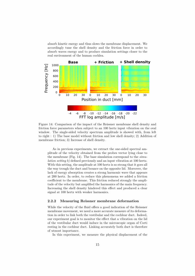
absorb kinetic energy and thus slows the membrane displacement. Weaccordingly tune the shell density and the friction force in order toabsorb waves energy and to produce simulation settings closer to thereal environment of the human cochlea.

-4 -6 -8 -10 -12 -14 -16 -18 -20 -22

0

200

400

600

800

1000

0 10 20 30 0 10 20 30 0 10 20 30

Base + Friction + Shell density

Position in duct [mm]

Frequency

[H

z]

FFT log amplitude [m/s]

Figure 14: Comparison of the impact of the Reissner membrane shell density andfriction force parameters when subject to an 100 hertz input vibration on the ovalwindow. The single-sided velocity spectrum amplitude is showed with, from leftto right : 1) The base model without friction and low shell density; 2) Addition ofmembrane friction; 3) Increase of shell density.

As in previous experiments, we extract the one-sided spectral am-plitude of the velocity obtained from the probes vector lying close tothe membrane (Fig. 14). The base simulation correspond to the simu-lation setting b) defined previously and an input vibration at 100 hertz.With this setting, the amplitude at 100 hertz is so strong that it goes allthe way trough the duct and bounce on the opposite lid. Moreover, thelack of energy absorption creates a strong harmonic wave that appearsat 200 hertz. In order, to reduce this phenomena we added a frictioncoefficient to the membrane. This friction reduced strongly the ampli-tude of the velocity but amplified the harmonics of the main frequency.Increasing the shell density hindered this effect and produced a clearsignal at 100 hertz with weaker harmonics.

2.2.2 Measuring Reissner membrane deformationWhile the velocity of the fluid offers a good indication of the Reissnermembrane movement, we need a more accurate measure of its deforma-tion in order to link both the vestibular and the cochlear duct. Indeed,our experiment goal is to monitor the effect that a vibration on the lidof the vestibular duct would induce in the microscopic organ of Cortiresting in the cochlear duct. Linking accurately both duct is thereforeof utmost importance.

In this experiment, we measure the physical displacement of the

15

membrane. For that, we have to remember that this membrane isrepresented by a set of membrane particles that freely evolve in a threedimensional space. More precisely, tenth of thousands of particles arerequired to correctly represent the membrane. Tracking such amountof particles over tenth of thousand of iterations is a daunting task : itwould require a large amount of memory.

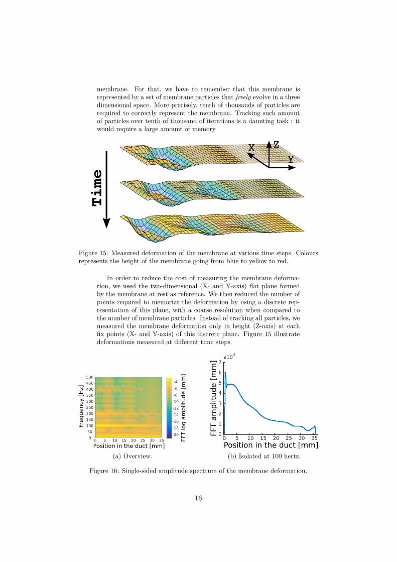
Figure 15: Measured deformation of the membrane at various time steps. Coloursrepresents the height of the membrane going from blue to yellow to red.

In order to reduce the cost of measuring the membrane deforma-tion, we used the two-dimensional (X- and Y-axis) flat plane formedby the membrane at rest as reference. We then reduced the number ofpoints required to memorize the deformation by using a discrete rep-resentation of this plane, with a coarse resolution when compared tothe number of membrane particles. Instead of tracking all particles, wemeasured the membrane deformation only in height (Z-axis) at eachfix points (X- and Y-axis) of this discrete plane. Figure 15 illustratedeformations measured at different time steps.

0 5 10 15 20 25 30 350

50

100

150

200

250

300

350

400

450

500

Position in the duct [mm]

Frequency

[H

z]

-20

-18

-16

-14

-12

-10

-8

-6

-4

FFT log a

mplit

ude [

mm

]

(a) Overview.

0 5 10 15 20 25 30 350

1

2

3

4

5

6

7x10

-2

FFT a

mp

litu

de [

mm

]

Position in the duct [mm](b) Isolated at 100 hertz.

Figure 16: Single-sided amplitude spectrum of the membrane deformation.

16

Using the previously defined realistic conditions, we memorized themembrane deformation in response to an input vibration at 100 hertz.The choice of this frequency was made in order to observe a deforma-tion all along the membrane. We extracted the central vector of de-formation measures in respect of the X-axis. We choose this measuresvector as it represented the biggest observed membrane deformationover time and analysed its one-sided spectrum amplitude.

Figure 16a shows an oscillation of the membrane at 100 hertz withweaker harmonics at 200 and 400 hertz. These observations corrobo-rate the one previously made on the fluid velocity. Figure 16a isolatesthe membrane displacement amplitude for the 100 hertz frequency.The amplitude starts with a value of 50 microns and reduces until theend of the membrane where it reaches a value of 10 microns. The orderof magnitude of this simulated deformation is in the same range as themeasured thickness of the Reissner membrane (5-15 microns [18]).

It is rather interesting to note that this amplitude begins to dropafter the structural chamber of the vestibular duct. In section 2.1.2, westipulated that the structural plateau in this region may act as a high-pass filter. And indeed, the major part of the deformation attenuationhappens in between 6 and 11−15 millimetres which roughly correspondto the end of the chamber and the start of the bump.

3 Simulation of the cochlear duct and theorgan of CortiIn the previous section, we have shown that periodic waves propagatingin the vestibular duct produce oscillation of the Reissner membrane ofequal frequencies. This membrane connects the vestibular duct to thecochlear duct. Therefore, this oscillation may well create fluid move-ments in the cochlear duct and propagate to the microscopic organ ofCorti. In this section, we enquire if such phenomena could happen andexplain how this organ micro-mechanics translates mechanical wavesinto nervous signals.

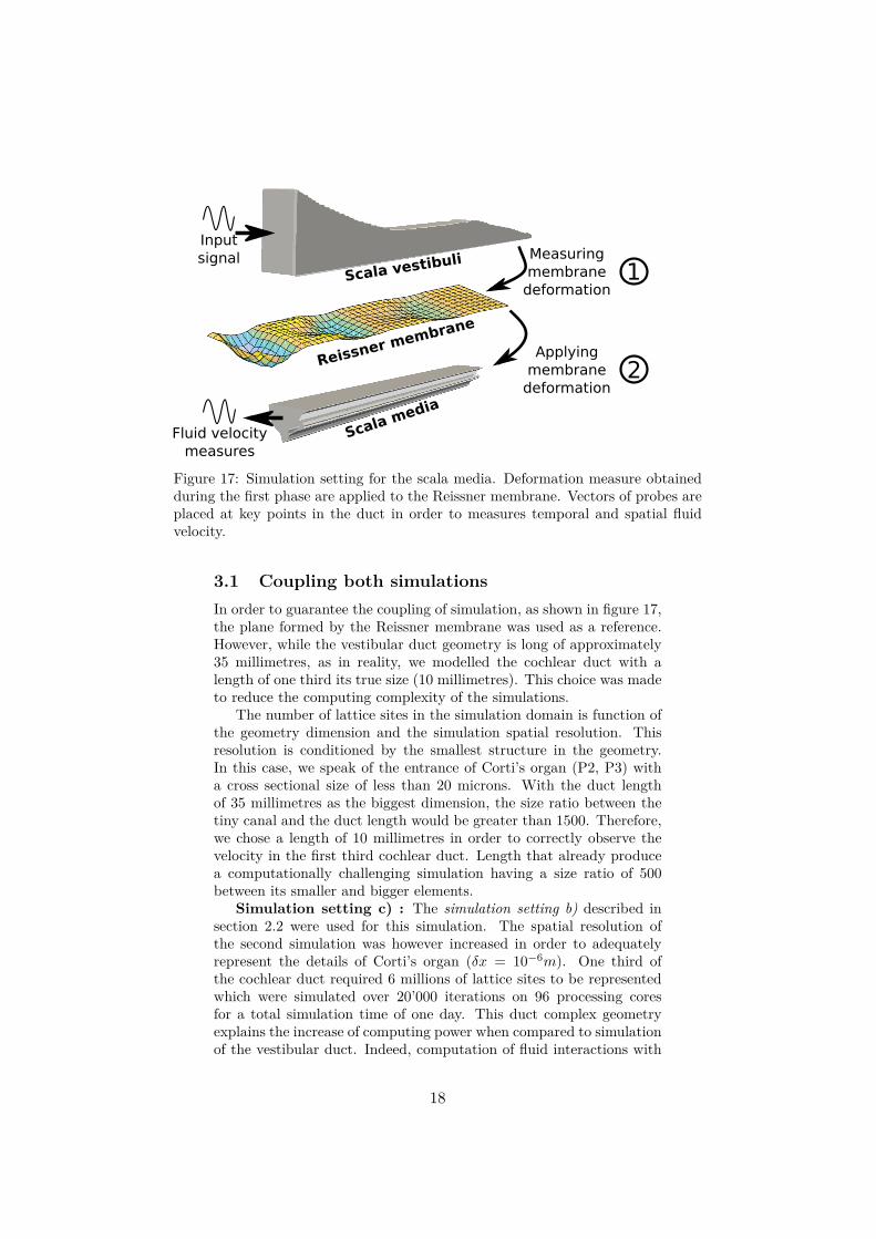
Figure 17 shows the two main steps of this experiment. The firstone correspond to the measures of the Reissner membrane deformationwith the simulation setting b) described in section 2.2. In the secondstep, we applied this deformation on the the geometry representing thecochlear duct.

However, this geometry, represented in figure 18, is far more com-plex than the one of the vestibular duct and thus was designed moreaccurately. Such level of detail was required to correctly simulated thefluid velocity inside the organ of Corti. Therefore this canal proportionand global aspect were carefully preserved during its conception. Thepoints of interest lies in the organ of Corti (P1), the scala media (P4)and the tiny canal linking both elements (P2, P3). Fluid velocity ofeach of these locations will therefore be measured.

17

Measuringmembrane

deformation

Applyingmembrane

deformation

Reissner membrane

Scala media

Scala vestibuliInputsignal

Fluid velocitymeasures

1

2

Figure 17: Simulation setting for the scala media. Deformation measure obtainedduring the first phase are applied to the Reissner membrane. Vectors of probes areplaced at key points in the duct in order to measures temporal and spatial fluidvelocity.

3.1 Coupling both simulationsIn order to guarantee the coupling of simulation, as shown in figure 17,the plane formed by the Reissner membrane was used as a reference.However, while the vestibular duct geometry is long of approximately35 millimetres, as in reality, we modelled the cochlear duct with alength of one third its true size (10 millimetres). This choice was madeto reduce the computing complexity of the simulations.

The number of lattice sites in the simulation domain is function ofthe geometry dimension and the simulation spatial resolution. Thisresolution is conditioned by the smallest structure in the geometry.In this case, we speak of the entrance of Corti’s organ (P2, P3) witha cross sectional size of less than 20 microns. With the duct lengthof 35 millimetres as the biggest dimension, the size ratio between thetiny canal and the duct length would be greater than 1500. Therefore,we chose a length of 10 millimetres in order to correctly observe thevelocity in the first third cochlear duct. Length that already producea computationally challenging simulation having a size ratio of 500between its smaller and bigger elements.

Simulation setting c) : The simulation setting b) described insection 2.2 were used for this simulation. The spatial resolution ofthe second simulation was however increased in order to adequatelyrepresent the details of Corti’s organ (δx = 10−6m). One third ofthe cochlear duct required 6 millions of lattice sites to be representedwhich were simulated over 20’000 iterations on 96 processing coresfor a total simulation time of one day. This duct complex geometryexplains the increase of computing power when compared to simulationof the vestibular duct. Indeed, computation of fluid interactions with

18

a) Organ of Corti

P1

P2

P3

b) Scala media

X

Z Y

Reissner membrane

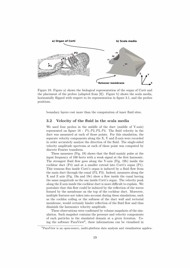
Figure 18: Figure a) shows the biological representation of the organ of Corti andthe placement of the probes (adapted from [9]). Figure b) shows the scala media,horizontally flipped with respect to its representation in figure 3.1, and the probespositions.

boundary layers cost more than the computation of inner fluid sites.

3.2 Velocity of the fluid in the scala mediaWe used four probes in the middle of the duct (middle of Y-axis)represented on figure 18 : P1, P2, P2, P4. The fluid velocity in theduct was measured at each of those points. For this simulation, theseparate velocity components along the X, Y and Z-axis were recordedin order accurately analyse the direction of the fluid. The single-sidedvelocity amplitude spectrum at each of these point was computed bydiscrete Fourier transform.

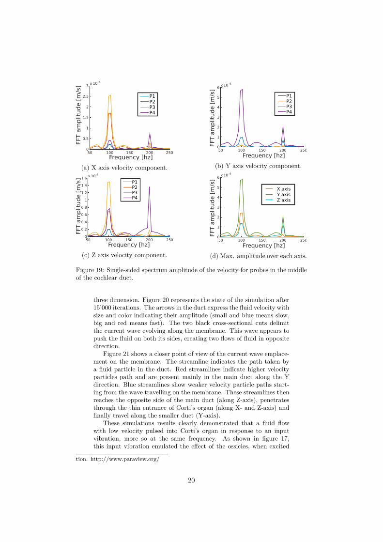
These measures (Fig. 19) shows that the fluid mainly pulse at theinput frequency of 100 hertz with a weak signal at the first harmonic.The strongest fluid flow goes along the Y-axis (Fig. 19b) inside thecochlear duct (P4) and at a smaller extend into Corti’s organ (P1).This tenuous flux inside Corti’s organ is induced by a fluid flow fromthe main duct through the canal (P2, P3). Indeed, measures along theX and Z axis (Fig. 19a and 19c) show a flow inside the canal havingthe same magnitude as the one inside Corti’s organ. The velocity peakalong the Z axis inside the cochlear duct is more difficult to explain. Wepostulate that this flow could be induced by the reflection of the wavesformed by the membrane on the top of the cochlear duct. Moreover,multiple features not taken into account during these simulations, suchas the cochlea coiling or the softness of the duct wall and tectorialmembrane, would certainly hinder reflection of the fluid flow and thusdiminish the harmonics velocity amplitude.

These observations were confirmed by volume snapshots of the sim-ulation. Such snapshot contains the pressure and velocity componentsof each particles in the simulated domain at a given iteration. Us-ing the software ParaView6, these informations can be visualised in

6ParaView is an open-source, multi-platform data analysis and visualization applica-

19

Frequency [hz]50 100 150 200 250

FFT a

mp

litu

de [

m/s

] x 10-4

0

0.5

1

1.5

2

2.5

3

P1P2P3P4

(a) X axis velocity component.

Frequency [hz]50 100 150 200 250

x 10-4

0

1

2

3

4

5

6

P1P2P3P4

FFT a

mplit

ude [

m/s

]

(b) Y axis velocity component.

50 100 150 200 250

x 10-4

0

0.2

0.4

0.6

0.8

1

1.2

1.4

1.6P1P2P3P4

Frequency [hz]

FFT a

mplit

ude [

m/s

]

(c) Z axis velocity component.Frequency [hz]

50 100 150 200 250

x 10-4

0

1

2

3

4

5

6

Z axis

X axisY axis

FFT a

mplit

ude [

m/s

]

(d) Max. amplitude over each axis.

Figure 19: Single-sided spectrum amplitude of the velocity for probes in the middleof the cochlear duct.

three dimension. Figure 20 represents the state of the simulation after15’000 iterations. The arrows in the duct express the fluid velocity withsize and color indicating their amplitude (small and blue means slow,big and red means fast). The two black cross-sectional cuts delimitthe current wave evolving along the membrane. This wave appears topush the fluid on both its sides, creating two flows of fluid in oppositedirection.

Figure 21 shows a closer point of view of the current wave emplace-ment on the membrane. The streamline indicates the path taken bya fluid particle in the duct. Red streamlines indicate higher velocityparticles path and are present mainly in the main duct along the Ydirection. Blue streamlines show weaker velocity particle paths start-ing from the wave travelling on the membrane. These streamlines thenreaches the opposite side of the main duct (along Z-axis), penetratesthrough the thin entrance of Corti’s organ (along X- and Z-axis) andfinally travel along the smaller duct (Y-axis).

These simulations results clearly demonstrated that a fluid flowwith low velocity pulsed into Corti’s organ in response to an inputvibration, more so at the same frequency. As shown in figure 17,this input vibration emulated the effect of the ossicles, when excited

tion. http://www.paraview.org/

20

Figure 20: Effect of the membrane deformation, present in between the two blackcut, on the fluid velocity. Arrows represents the fluid velocity direction. Their sizeand color,from small blue to big red, indicate the velocity amplitude.

by sound, on the oval window. Such vibrations then propagated me-chanic waves through the perilymph of the vestibular duct inducing anoscillation of the Reissner membrane. This oscillation, preserving theinput frequency, created a fluid flow in the cochlear duct that pulsedwith low velocity at the exact position of the hair cells.

In this scenario, the Reissner membrane plays a central role byrelaying the initial vibrations imposed to the oval window into thecochlear duct. This, by itself, contravene the implicitly and widelyaccepted scenario in which the Reissner membrane doesn’t affect thefluid flow between the vestibular and cochlear duct. Indeed, removingthis elastic membrane would strongly impact the dynamic of the fluidflow.

4 Discussion and Conclusion4.1 Inner ear mechanismOne of the inner ear function is to transform the sound that surroundsus into nervous signals. This mechanism is decomposed in multiplesteps starting from the vibration of the tympanic membrane. Thesevibrations are amplified by the ossicles and transmitted to the liquidfilled vestibule through the oval windows. The induced fluid wavesgenerate a vibratory response in the cochlea. This vibratory response isattributed to the difference of pressure in the oval and round windowsthat would create a travelling wave on the basilar membrane. Thistravelling wave activate then hair cells, or stereocila, present in Corti’sorgan due to its closeness with the basilar membrane [24].

This simplistic scenario minimizes the potential function of the un-dervalued Reissner membrane [15]. Recently, this membrane has beenshown to propagate travelling waves with amplitude comparable tothe one of the basilar membrane [16]. We simulated this phenomenaby applying vibrations at the entrance of the vestibular duct. Thesevibrations propagated waves inside the duct, thus deforming the Reiss-ner membrane. The oscillation of the membrane maintained the input

21

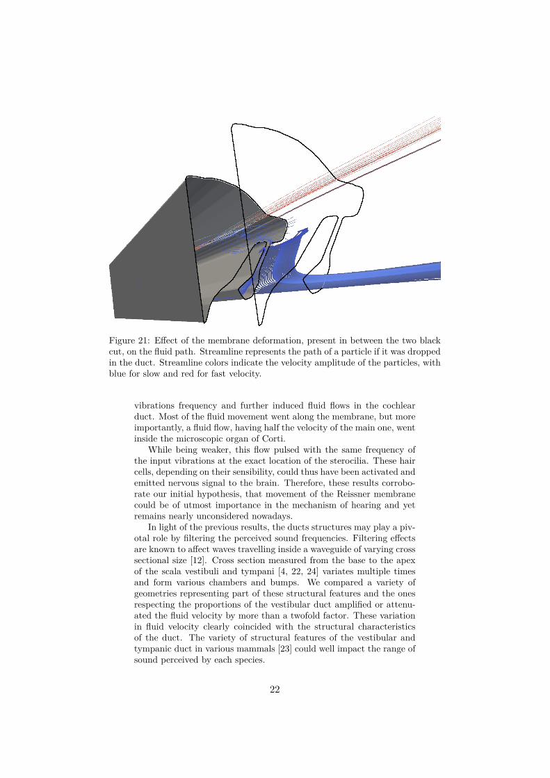
Figure 21: Effect of the membrane deformation, present in between the two blackcut, on the fluid path. Streamline represents the path of a particle if it was droppedin the duct. Streamline colors indicate the velocity amplitude of the particles, withblue for slow and red for fast velocity.

vibrations frequency and further induced fluid flows in the cochlearduct. Most of the fluid movement went along the membrane, but moreimportantly, a fluid flow, having half the velocity of the main one, wentinside the microscopic organ of Corti.

While being weaker, this flow pulsed with the same frequency ofthe input vibrations at the exact location of the sterocilia. These haircells, depending on their sensibility, could thus have been activated andemitted nervous signal to the brain. Therefore, these results corrobo-rate our initial hypothesis, that movement of the Reissner membranecould be of utmost importance in the mechanism of hearing and yetremains nearly unconsidered nowadays.

In light of the previous results, the ducts structures may play a piv-otal role by filtering the perceived sound frequencies. Filtering effectsare known to affect waves travelling inside a waveguide of varying crosssectional size [12]. Cross section measured from the base to the apexof the scala vestibuli and tympani [4, 22, 24] variates multiple timesand form various chambers and bumps. We compared a variety ofgeometries representing part of these structural features and the onesrespecting the proportions of the vestibular duct amplified or attenu-ated the fluid velocity by more than a twofold factor. These variationin fluid velocity clearly coincided with the structural characteristicsof the duct. The variety of structural features of the vestibular andtympanic duct in various mammals [23] could well impact the range ofsound perceived by each species.

22

4.2 Simulations limitations and challengesWhile striving to emulate the human ear conditions, our simulationsremained far from the reality. While we linked the vestibular andcochlear duct using the Reissner membrane, during the separate sim-ulation steps, the membrane was surrounded on one side by a fluidmimicking the perilymph and by air on the other side. The impactof this inaccurate setting was minimized by increasing the density andfriction of the membrane. However, these required simplifications cre-ated a gap between our model and the real environment of the cochlea.

Accurately simulating the cochlea poses serious challenges for mul-tiple reasons. One of them resides in the complex structure and anatomyof the inner ear. Despite the recent progress in high-resolution medicalimaging, soft tissues such as the Reissner membrane remains hard toobserve and measure accurately [4, 18]. Assuming that these issueswill be fixed in the future, fully accurate geometries will then causeconsiderable computational challenges for CFD solvers.

The frequencies range and the scale of geometry details featured inthe cochlea leads to hardly tractable computational task. Simulatinglow and high frequency at the same time requires to chose a timeresolution that enable the sampling of the fastest frequency and a runtime long enough for the lowest frequency to propagate. Sampling 20points per period of a 20’000 hertz signal requires a time step of 5·10−6

seconds. With such time step, 104 iterations would be necessary to justgenerate one period of a 20 hertz signal. The same observation appliesto the spatial resolution of the geometry. As example, Corti’s organ hasgeometric features of less than 10 microns, while the unrolled lengthof the cochlea is greater than 30 millimetres.

The spatial and temporal resolutions of our simulation of one thirdof the cochlear duct already required a one day runtime with 96 pro-cessors to generate enough data. This small simulation, in regard tothe entire cochlea, was not even computing forces on the membranesince we applied its previously memorized deformation. Yet tenth ofthousands of particles were used to represent accurately the membrane.Adding the resolution of forces on the entire Reissner and basilar mem-brane would consequently increase the required computational power.

Hopefully, advances in CFD will help address these issues. Multi-domains methods [13, 20] are a first example of such methods. Theyaim to facilitate the simulation of geometries showing structure withmultiple scales of dimensions by dividing the simulation domain inblocks having each an appropriate spatial resolution. Another issuecomes from immersed elastic membrane. Such complex fluid-solid in-teractions are complex to address with the Lattice-Boltzmann methodand are subject to recent advances [6].

In addition to these CFD improvements, a direct solution to thischallenging computational task would be to use the already availablecomputing resources. Palabos is known to manage simulation on clus-ters having several thousands of processors7.

7LEMANICUS Blue Gene/Q Supercomputer : http://bluegene.epfl.ch/

23

4.3 ConclusionIn conclusion, by simulating the full path of mechanical waves createdby vibrations of the oval window, we showed that the Reissner mem-brane could well play an important role in the activation of hair cellspresent in the microscopic organ of Corti. In this context, the structureof cochlea ducts presented significant frequency filtering properties bymodifying wave velocity by up to a twofold factor.

In order to simulate these phenomenon, we used a highly parallelCFD solver, Palabos. While these experiments where not fully realisticin regard of the human cochlea, they present an important step towardthe simulation of inner ear micro- and macro-mechanics. Novel CFDmethods coupled with the increasingly accurate measures of the humanear will allow in a near future to conceive truly realistic cochlea models.Given that the required computing resources are already us availablefor such computational challenge, we only are a few steps away ofrealising the crucial tool that would help us better understand thehuman hearing mechanism.

References[1] Bekesy, Georg V. “The Variation of Phase Along the Basi-

lar Membrane with Sinusoidal Vibrations.” The Journal of theAcoustical Society of America 19, no. 3 (May 1, 1947): 452–60.doi:10.1121/1.1916502.

[2] Bekesy, Georg von, and Ernest Glen Wever. Experiments in Hear-ing. New York: McGraw-Hill, 1960.

[3] Bohnke, F., and W. Arnold. “Nonlinear Mechanics of the Organ ofCorti Caused by Deiters Cells.” IEEE Transactions on Bio-MedicalEngineering 45, no. 10 (October 1998): 1227–33.

[4] Braun, K., F. Bohnke, and T. Stark. “Three-Dimensional Repre-sentation of the Human Cochlea Using Micro-Computed Tomog-raphy Data: Presenting an Anatomical Model for Further Numer-ical Calculations.” Acta Otolaryngol 132, no. 6 (2012): 603–13.

[5] Elliott, Stephen J., and Christopher A. Shera. “The Cochlea as aSmart Structure.” Smart Materials & Structures 21, no. 6 (June2012): 64001.

[6] Favier, Julien, Alistair Revell, and Alfredo Pinelli. “A LatticeBoltzmann–Immersed Boundary Method to Simulate the FluidInteraction with Moving and Slender Flexible Objects.” Journalof Computational Physics 261 (March 15, 2014): 145–61.

[7] Geisler, C. Daniel, and Chunning Sang. “A Cochlear Model UsingFeed-Forward Outer-Hair-Cell Forces.” Hearing Research 86, no.1–2 (June 1995): 132–46.

[8] Givelberg, Edward, and Julian Bunn. “A Comprehensive Three-Dimensional Model of the Cochlea.” Journal of ComputationalPhysics 191, no. 2 (2003): 377–91.

24

[9] Gray, Henry. Anatomy of the Human Body. Philadelphia: Lea &Febiger, 1918.

[10] Huber, Christian, Babak Shafei, and Andrea Parmigiani. “A NewPore-Scale Model for Linear and Non-Linear Heterogeneous Dis-solution and Precipitation.” Geochimica et Cosmochimica Acta124 (January 1, 2014): 109–30.

[11] Kemp, David T. “Otoacoustic Emissions, Their Origin in CochlearFunction, and Use.” British Medical Bulletin 63, no. 1 (October1, 2002): 223–41.

[12] Kinsler, Lawrence E, Austin R Frey, Alan B Coppens, and JamesV Sanders. “Fundamentals of Acoustics.” Fundamentals of Acous-tics, 4th Edition, by Lawrence E. Kinsler, Austin R. Frey, Alan B.Coppens, James V. Sanders, Pp. 560. ISBN 0-471-84789-5. Wiley-VCH, December 1999. 1 (1999).

[13] Lagrava, D., O. Malaspinas, J. Latt, and B. Chopard. “Advancesin Multi-Domain Lattice Boltzmann Grid Refinement.” Journal ofComputational Physics 231, no. 14 (May 20, 2012): 4808–22.

[14] Manoussaki, D., and R. Chadwick. “Effects of Geometry on FluidLoading in a Coiled Cochlea.” SIAM Journal on Applied Mathe-matics 61, no. 2 (January 1, 2000): 369–86.

[15] Ni, Guangjian, Stephen J. Elliott, Mohammad Ayat, and Paul D.Teal. “Modelling Cochlear Mechanics.” BioMed Research Interna-tional 2014 (July 23, 2014): e150637.

[16] Reichenbach, Tobias, Aleksandra Stefanovic, Fumiaki Nin, and A.J. Hudspeth. “Waves on Reissner’s Membrane: A Mechanism forthe Propagation of Otoacoustic Emissions from the Cochlea.” CellRep 1, no. 4 (April 2012): 374–84.

[17] Robles, Luis, and Mario A. Ruggero. “Mechanics of the Mam-malian Cochlea.” Physiological Reviews 81, no. 3 (July 2001):1305–52.

[18] Shibata, Takashi, Sumiko Matsumoto, Tetsuzo Agishi, and TeikoNagano. “Visualization of Reissner Membrane and the Spiral Gan-glion in Human Fetal Cochlea by Micro-Computed Tomography.”American Journal of Otolaryngology 30, no. 2 (2009): 112–20.

[19] Steele, Charles R., Jacques Boutet de Monvel, and Sunil Puria. “AMULTISCALE MODEL OF THE ORGAN OF CORTI.” Journalof Mechanics of Materials and Structures 4, no. 4 (2009): 755–78.

[20] Touil, Hatem, Denis Ricot, and Emmanuel Leveque. “Direct andLarge-Eddy Simulation of Turbulent Flows on Composite Multi-Resolution Grids by the Lattice Boltzmann Method.” Journal ofComputational Physics 256 (January 1, 2014): 220–33.

[21] Ulfendahl, Mats. “Mechanical Responses of the MammalianCochlea.” Progress in Neurobiology 53, no. 3 (October 1997):331–80.

[22] Wysocki, Jaros aw. “Dimensions of the Human Vestibular andTympanic Scalae.” Hearing Research 135, no. 1–2 (1999): 39–46.

25

[23] Wysocki, Jaros aw. “Dimensions of the Vestibular and TympanicScalae of the Cochlea in Selected Mammals.” Hearing Research161, no. 1 (2001): 1–9.

[24] Yost, William A, and DW Nielsen. ”Fundamentals of Hearing”.Holt, Rinehart, and, 1989.

[25] Zeng, Fan-Gang, and Richard R. Fay. Cochlear Implants: Audi-tory Prostheses and Electric Hearing. Springer Science & BusinessMedia, 2013.

[26] Zimny, Simon, Bastien Chopard, Orestis Malaspinas, Eric Lorenz,Kartik Jain, Sabine Roller, and Jorg Bernsdorf. “A Multiscale Ap-proach for the Coupled Simulation of Blood Flow and ThrombusFormation in Intracranial Aneurysms.” Procedia Computer Sci-ence, 2013 International Conference on Computational Science,18 (2013): 1006–15.

[27] Zwislocki, J. J. “Cochlear Waves: Interaction between Theory andExperiments.” The Journal of the Acoustical Society of America55, no. 3 (March 1, 1974): 578–83.

26