Embed Size (px)
Citation preview

Study of Electron-Impact Induced Fragmentation
of Thymine
Francis Anthony Mahon
A thesis submitted for the degree of Masters of Science
Department of Experimental Physics
N.U.I. Maynooth
Maynooth
Co.Kildare
May 2013
Head of Department
Professor J. Anthony Murphy
Research Supervisor
Dr. Peter J. M van der Burgt

Contents
Abstract i
Acknowledgements ii
Chapter 1. Introduction
1.1. Radiation damage to DNA 1
1.2. Low energy electrons in DNA damage 5
1.3. Dissociative electron attachment (DEA) 6
1.4. Experiments in thymine 9
1.4.1 DEA 9
1.4.2 Bond selective DEA 10
1.4.3 Electron impact on thymine 14
1.4.4 Photon impact on thymine 15
1.4.5 Proton impact on thymine 18
1.4.6 Ion impact on thymine 20
1.5. Maynooth research 21

Chapter 2. Principles and Instrumentation of Mass Spectrometry
2.1. What is Mass spectrometry? 23
2.2. Mass filters 24
2.3. Mass spectrometry using traps 26
2.4. Time-of-flight mass spectrometry 27
Chapter 3. Experimental setup
3.1. General overview of the experiment 32
3.2. The expansion chamber 34
3.3. The collision chamber 37
3.3.1. The electron gun and faraday cup 37
3.3.2. The electron gun voltage box 40
3.4 . The reflectron chamber 41
3.5. The interlock system 43

Chapter 4. Interfacing, Data acquisition and Data analysis software
4.1. Introduction 44
4.2. Amplifier and timing discriminator 45
4.3. Pulsing and timing 46
4.4. Multichannel scalar card 49
4.5. LabVIEW programs 51
4.5.1. Testing the electron gun 51
4.5.2. Acquiring single mass spectra 53
4.5.3. Acquiring multiple mass spectra 55
4.5.4. Gaussian Peak fitting 57
Chapter 5. Test measurements with thymine
5.1. Comparison of LabVIEW programs to MCS 61
5.2. Calibration of electron gun 63
5.3. Calibration of mass spectra 65
5.4. Analysis of water peaks 67
5.5. Oven tests 71
5.5.1. Oven temperature 71
5.5.2 Oven depletion 72

Chapter 6. Electron impact fragmentation of thymine
6.1. Introduction 77
6.2. Relative yield comparison 78
6.3. Identification of the thymine peaks 79
6.4. Thymine Excitation functions 83
6.4.1. The 26-29 u group 83
6.4.2. The 36-40 u group 84
6.4.3. The 41-45 u group 85
6.4.4. The 51-56 u group 86
6.4.5. The 70-72 u group and the 82-84 u group 87
6.4.6. The 97u and the 124-127 u group 89
6.5. Appearance energies 91
6.6. Total ionisation cross sections 97
6.7. Background contribution 98
Chapter 7. Conclusion 99
References 101
Appendix 106

Abstract
The aim of the experiment described in this thesis was to generate a molecular beam
of thymine and to investigate the fragmentation processes induced by low-energy
electron impact. A molecular beam of thymine is generated by placing thymine in
powder form inside a resistively heated oven. The beam of thymine is then crossed by
a pulsed electron beam from an electron gun that consists of four electrostatic lens
elements and a deflection system for steering the beam. A reflectron time-of-flight
mass spectrometer with a microchannel plate detector is used to detect and mass
resolve the positively charged fragments. LabVIEW based data acquisition techniques
are used to accumulate the time-of-flight data as a function of electron impact energy.
The work described in this thesis is based on a single data set of thymine with electric
impact energy varied from 0.5 to 99.7 eV in steps of 0.5 V. To determine the yield of
the various fragment ions, groups of peaks were fitted with a sequence of normalised
Gaussian peaks using a specially developed LabVIEW program. Using this program the
fitting of the peaks was done automatically for all electron energies. Excitation
functions for the most positively ionised fragments have been extracted/or determine
and their appearance energies have been determined and compared to current
research on thymine. Because all excitation functions have been generated from this
single data set and assuming that the detection efficiency of the RTOFMS is mass
independent, the yield of all fragments are on the same relative scale and are
comparable. Total ionisation cross sections have been obtained for our data set and
are in good agreement with theoretical calculations.

1
CHAPTER 1
Introduction
1.1 Radiation damage of DNA
In recent years a lot of research has focused on the interaction of low energy electrons
with biomolecules such as the DNA bases, after experiments in Leon Sanche’s group in
Sherbrooke (Canada) showed that low energy electrons are very effective in causing
DNA strand breaks [1]. Of the secondary species generated when high-energy ionizing
radiation interacts with living cells, low energy electrons (with energies less than 20
eV) are the most abundant [2].
Experimental techniques such as mass spectrometry and electron spectroscopy are
being used in many laboratories to study the building blocks of biomolecules in the gas
phase [3-5]. These techniques allow detailed information on the properties of
molecules and the dynamics of reactions to be explored.
Biological effects on a cell can result from both direct and indirect action of radiation.
Direct effects such as a strand break in DNA are produced by the initial action of the
radiation itself and indirect effects are caused by the later chemical action of free
radicals and other secondary radiation products. An example of an indirect effect is a
strand break that results when an OH radical attacks a DNA sugar at a later time
(between about 10-12 s and 10-9 s) [6]. Depending on the dose and the type of
radiation, the biological effects of radiation can differ widely. Some effects can occur
rapidly while others may take years to become evident. The types of DNA damage
produced by radiation can be broadly classified as single-strand breaks, double-strand
breaks and base damages. These structural changes and errors in their repair can lead
to gene mutations and alterations in the chromosome. Presently, a great deal is
understood about damage repair and misrepair in DNA and its relation to potential

2
tumor induction, but how a cell operates to deter or prevent the transmission of
genetic damage is still largely an open question. Molecular genes at specific stages of
the cell reproductive cycle appear to recognise and react to the management and
repair of damaged DNA. [7]
For genetic alterations to occur in a cell, the cell nucleus must be traversed by a
charged-particle track. Nearby cells called bystanders can also sustain genetic damage,
even though no tracks pass through them and they receive little or no radiation dose.
In some systems, a small dose of radiation triggers a cellular response that protects
the cells from a larger dose of radiation. Radiation used to protect biological material
is being successfully practiced in tumor therapy. The problem in tumor therapy is to
only expose the cancerous material while keeping all other areas unirradiated. One
method of treatment uses radiosensitisers with the effect that the sensitised
cancerous cells will be destroyed with radiation dosages that leave the healthy
material essentially unaffected.
The most important component of the cell nucleus is Deoxyribonucleic acid (DNA).
This is the part of the cell nuclei where genetic information is stored. DNA is a
biopolymer consisting of two strands containing the 4 heterocyclic bases, thymine (T),
adenine (A), cytosine (C) and guanine (G). Each of these bases are bound to the DNA
backbone which itself is composed of phosphate and sugar units. Both strands of the
DNA are connected through reciprocal hydrogen bonding between pairs of bases in
opposite positions. The geometry is such that, adenine pairs with thymine (AT) and
guanine with cytosine (GC). [7]

3
Figure 1.1. Helical Structure of DNA including the DNA bases adenine (A), thymine (T),
cytosine (C) and guanine (G) [7]
The structure of the thymine molecule studied in this thesis is shown in figure 1.2
Figure 1.2. Structure of the thymine molecule. [8]

4
In order to understand the effect of high energy radiation on DNA, one must consider
this interaction in terms of its chronological sequence. Consider a beam of protons at
energies in the keV - MeV range. The primary photon interaction either absorption or
scattering, removes electrons from essentially any occupied state. These can range
from valence orbitals to core levels. Depending on the energy of these ionized
electrons, they induce further ionization events thereby losing energy and slowing
down. These electrons are usually assigned as secondary although they are the result
of primary, secondary and tertiary interactions [7]. The estimated quantity is 104
secondary electrons per 1 MeV primary quantum [10].
The sequence described above can involve any of the cell components (DNA, water,
proteins) separately or in any combination. Water is the most abundant component of
a cell and generates the reactive OH radical which can attack any cell component in its
surrounding. It is assumed that damage of the genome in a living cell by ionizing
radiation is about one third direct and two third indirect. [11]
Direct damage concerns energy deposition and reactions directly in the DNA and its
closely bound water molecules. Indirect damage concerns energy disposition in water
molecules and the other biomolecules in the vicinity of the DNA. Most of the indirect
damage is believed to occur from the attack by the highly reactive hydroxyl radical OH.
[6]
There are three major processes and reactions that occur in the molecular network of
a living cell. [9]
(i) The physical stage. This refers to processes and reactions in the fs and ps time
frame after the primary interaction. In this time frame, electronic excitation and
ionization occur along with subsequent bond ruptures to create radicals like OH and
also an abundant number of secondary electrons.

5
(ii) The chemical stage. This includes molecular relaxation which involves multiple
bond cleavages and the subsequent formation of new molecules. At this stage, free
radicals take part in an array of reactions which include enzymatic repair and rejoining
of DNA breaks that reduce the initial damage that can occur in the physical stage.
(iii) The biological stage. This stage refers to the changes occurring on a longer time
scale, including the overall response of the system which could extend over a time
range of several years. Cell functions can be affected within minutes. The majority of
DNA strand breaks are repaired but, the unrepaired strands lead to cell death. Some
of the damage to the DNA might not induce cell death but can pass mutations on to
the daughter cells.
1.2 Low energy electrons in DNA damage
High energy quanta generate large amounts of electrons at initial energies up to some
tens of eV. It is these electrons that are responsible for triggering the reactions that
are relevant to direct damage of DNA. Low energy electrons (<10 eV) are especially
responsible for strand breaks in DNA.
Single strand (SSB) breaks occur when one of the two backbones is broken. To repair
damage to one of the two paired molecules, there exist a number of excision repair
mechanisms that remove the damaged nucleotide and replace it with an undamaged
one. There are three pathways that exist to repair single strand breaks, these are base
excision repair, nucleotide excision repair and mismatch repair [12].
When two chains are broken within a short distance, the damage is referred to as a
Double strand break (DSB). The DSB damage is difficult for the cell to repair and
without reparation the cell can mutate or eventually die. Three mechanisms exist for
repair of DSB [13], [14].

6
The role low energy electrons would have in DNA damage became more evident after
experiments conducted by Sanche and co-workers in 2000 [10]. The group used an
electron beam over the energy range of 3–30 eV to irradiate plasmid DNA. They
observed the appearance of SSB and DSB at energies above 15 eV, with strand breaks
continuously increasing as a function of electron energy. Most notably, they observed
SSB and DSB in the range below the ionization threshold (<10 eV). Further
experimentation by Sanche and co-workers [15] in 2004, saw the electron energy
being brought down to a range of 0-3 eV where strand breaks were detected at 3 eV
and peaking at 0.8 eV. Although at this low range, the resonances were found to be
solely associated with DSB. These finding were completely unexpected, because
before 2004 it was believed that only electrons at energies above the isolation
threshold could damage DNA.
1.3 Dissociative Electron Attachment (DEA)
At low energies, below the electronic excitation level, electrons can be captured by
molecules into transient negative ions which subsequentially decompose into several
fragments. This process is called dissociative electron attachment (DEA), and
schematically it can be written as:
This process is initiated when an electron becomes temporarily trapped in a resonant
state of a molecule. This resonance can either decay by the emission of the extra
electron (auto detachment), leaving the molecule in the ground state or in a
vibrationally exited state, or it can dissociate in the same manner as the above
equation. The dissociation will only occur if the electron energy is sufficient and the
resonance is long lived. Burrow et al [16] have attributed the sharp peaks observed in
the DEA cross sections of uracil and thymine at energies below 3 eV to vibrational
Feshback resonances, in which the electron is weakly bound to a vibrationally excited

7
level of the molecule. Hotop et al [17] have reviewed experimental investigations of
resonance and threshold phenomena occurring in low energy electron collisions with
molecules, at electron energies below 1 eV.
DEA experiments were conducted in 2003 by Pan et al [18]. Two types of DNA sample
were bombarded with low energy electrons: synthetic 40-base-pair linear DNA and
natural plasmid DNA which was purified from bacteria. The linear DNA was formed
from complementary oligonnucleotides, 40 nucleotides in length, purified by
polyarcylamide gel electrophoresis [18]. Once the samples were prepared, they were
transferred to a rotary target holder housed in an UHV chamber via a gate valve. The
samples were irradiated by an electron gun producing a beam of 1.5 nA on a 4 mm2
spot with an energy spread of 0.5 eV full width at half maximum. Pan et al [18]
demonstrated that DEA is involved in low energy electron induced DNA damage, and
exhibits a maximum intensity around 9-9.5 eV. This is close to the maximum in the
yields of SSB and DSB induced by the low energy electrons on DNA. DEA is therefore
not limited to small molecules, but can also occur in extremely large molecules which
induce fragmentation and produce anions and radicals. The results reported from this
experiment indicate that H produced from DEA to DNA arises principally from the
bases and the sugar ring of the backbone whereas O is produced from fragmentation
in the backbone. The main results are shown in figure 1.2. The incident electron
energy dependence of the H, O and OH yields from 40-base-pair DNA is represented
as A in figure 1.3. They exhibit a single broad peak near 9 eV with a continuous rise at
higher energies. Low energy electron bombardment of natural DNA is represented as
curve B and they exhibit the same characteristics as shown in A. Curves C, D and E
exhibit the H yield functions from films of thymine, amorphous ice and α-
tetrahydrofuryl alchohol [18]. These curves indicate that DEA to the ring is the main H
desorption pathway, but the H peak energy from amorphous ice in curve D is too low
to be associated with DEA.

8
Figure 1.2. Incident electron energy dependence of H yields from thin films of: A) double stranded DNA, B) supercoiled plasmid DNA, C) thymine, D) amorphous ice and E) ribose
analog [18]. The dependence of the magnitude of the H signal on time of exposure to the electron beam is shown by the open squares in the upper right inset. The solid line is an exponential fit to the data.

9
1.4 Experiments in thymine
This section outlines the fragmentation pathways that occur in thymine and details
the major experiments that have been conducted using thymine and the results
obtained. Experiments using techniques such as electron impact via DEA or ionization,
ion impact, photon impact and collision experiments with clusters are also described.
A brief overview of research and goals for this project is also detailed in section 1.5.
1.4.1 DEA
DEA experiments were conducted by Heuls et al [19]. They measured the electron
energy dependence for production of anion fragments, induced by resonant
attachment of subionisation electrons to thymine and cytosine. Their measurements
suggest that this resonant mechanism may relate to critical damage of irradiated
cellular DNA by subionisation electrons prior to thermalisation.
In 2003, Denifl et al [20] conducted an experiment to study DEA to thymine using an
electron/molecule beam apparatus where the electron beam was formed in a custom
built hemispherical electron monochromator with a resolution of 30 meV. In their
measurements they could not observe the negative thymine parent ion (T) but they
observed the dominant (TH) resonance at 1.05 eV followed by a peak at 1.48 eV
and a broad resonance at 1.75 eV. Further advancements in the study of DEA were
made by S. Denifl and his team in 2004 [21]. They studied DEA to isolated gas-phase
cytosine (C) and thymine (T) and identified the resulting fragments, using a crossed
electron beam instrument combined with a quadrupole mass spectrometer. The team
discovered again that electron attachment to C and T leads to dissociation into the
various fragments without any hint of the C and T parent anions.

10
For thymine the following 9 fragments were observed within the energy range of 0 to
14 eV [20]:
(125 u)
(124 u)
(97 u)
(71 u)
(68 u)
(54 u)
(42 u)
(26 u)
(16 u)
It is noted here that (TH) indicates the negative ion formed by the detachment of a
single proton from the parent thymine molecule. Likewise, (T2H) indicates the
detachment of a hydrogen atom and a proton from the thymine molecule. This
notation, which is contrary to standard chemical notation, is commonly used in this
research field. Other DEA experiments were conducted by Heuls et al [21]. They
measured the electron energy dependence for production of anion fragments,
induced by resonant attachment of subionisation electrons to thymine and cytosine.
Their measurements suggest that this resonant mechanism may relate to critical
damage of irradiated cellular DNA by subionization electrons prior to thermalization.
1.4.2 Bond Selective DEA
S. Ptasinska et al [22] studied electron attachment to thymine in the electron energy
range 0-15 eV. The formation of fragment anions that are formed by the loss of one or
two H atoms is analysed as a function of incident electron energy. In their
experimental setup, an effusive beam of neutral molecules is produced by evaporating

11
thymine power in a resistively heated oven up to a temperature of 430 K. Gas phase
molecules are introduced through a 1 mm diameter capillary into the collision
chamber where they are crossed with a well defined beam of electrons that originate
from a hemispherical electron monochromator (HEM). The electrons are produced by
a hairpin filament and are accelerated with lens system into a hemispherical
electrostatic field analyser. Anions that are formed via electron attachment reactions
are extracted by a weak electric field towards the entrance of a quadrupole mass filter
where the mass per charge ratio of the anions are analysed.
A) DEA yielding (T-H)
They suggest that the dominant negative ions formed via DEA to nucleobases are the
closed-shell dehydrogenated molecular anions. For thymine the reaction pathway is:
In thymine, the reaction above can occur at four different positions: 1N, 3N, 6C or at
the carbon atom of the methyl group. The values of the bond dissociation energies
(BE) required for the removal of one H atom from the neutral thymine molecule and
the electron affinities of the corresponding (T-H) isomers are shown in table 1.1
below.
Bond BE EA BE-EA
1N-H 4.29 3.4 0.89
3N-H 5.8 4.5 1.3
CH2-H 4.54 1.82 2.23
6C-H 4.98 2.76 2.72
Table 1.1. The values of the bond dissociation energies (BE) and electron affinities (EA) of the corresponding (T-H) isomers [22]

12
The ion efficiency curve for the mass 125u (T-H) in the range of 0 to 4 eV is shown in
figure 1.4. This figure also includes the ion efficiency curve for the partially deuterated
thymine masses 129 u (TD-H) and 128 u (TD3-H). The electron energy resolution for
thymine was 60 meV.
Figure 1.4. ion efficiency curve for the masses (a) 129 u (TD-H), (b) 128 u (TD3-H) and (C) 125u (T –H) [22].
B) DEA yielding H
The formation of H is observed and investigated by S. Ptasinska et al [22]. The
reaction channel is shown below.

13
This anion was produced in the energy range 5 to 13 eV. In this range, the desorption
of H from thin films of isolated DNA compounds and single and double strand break
formation were observed. The anion yield of H exhibits 3 clearly separated peaks
centered at 5.5, 6.8 and 8.5 eV. The 5.5 eV peak can be ascribed to the H loss from
the 1N position. The 6.8 eV peak comes from the H loss from the 3N nitrogen atom
and the 8.5 eV peak represents the H loss from the 6C position.
C) DEA yielding (T-2H)-
Site selectivity was also observed for the 124 u mass. The ion yield exhibits a well-
pronounced narrow resonance close to 0 eV followed by a weak resonance at 1.5 eV.
A broad structure of overlapping resonances at electron energies above 6 eV. The two
hydrogen atoms that are removed from thymine may be lost as two independent
atoms
or as an intact hydrogen molecule but the binding energy of H2 reduced the required
energy by 4.54 eV
The minimum energies required for the removal of either two individual H atoms or
one H2 molecule are determined using high-level quantum-chemical calculations.
More bond selective DEA experiments have been conducted by S. Ptasinska et al [23],
[24] and Abdoul-Carime et al [25]

14
1.4.3 Electron impact on thymine
Rice et al [26] study the fragmentation patterns of thymine by recording spectra at
low electron beam energies in addition to the standard 70 eV. The solid compounds
were introduced directly into the ion source of a double-focusing mass spectrometer.
To generate a sufficiently high vapor pressure, the vicinity of the ion source was
heated to 200 oC. Mass spectra were recorded at electron impact energies of 70 and
20 eV. They identified the molecular ion peak at 126 u and intense fragment ion peaks
at 83 and 55 u corresponding to the loss of HNCO. Decarbonylation of deuterated 83 u
is followed by loss of either a hydrogen or a deuterium atom.
Imhoff et al [27] use 70 eV electron impact to study both thymine and thymine-
methyl-d3-6-d in the gas phase. A large amount of thymine was deposited on a Pt
substrate, which is then placed in front of the entrance of a quadrupole mass
spectrometer. The thymine molecules are then evaporated from the Pt into the
quadrupole mass spectrometer by warming the Pt substrate to 89-95 oC and subjected
to electron impact. The positive ion fragmentation from thymine produced by 70 eV
electron impact is shown in figure 1.5 (a). They observed that the 83 u fragment which
formed from the loss of HCNO group from thymine was found to shift to 87 u in the
case of thymine-methyl-d3-6-d indicating that it contains the four deuterium atoms.
Further loss of a hydrogen atom gives the 82 u fragment which shifts to 85 u in the
mass spectrum of thymine-methyl-d3-6-d as a result of further loss of carbon-bound
deuterium.
Shafranyosh et al [28] used a crossed molecular and electron beam to study the
electron impact on thymine and determine the energy dependencies and absolute
values of total cross sections for the formation of positive and negative ions of
thymine molecules. They found that the maximal cross section for the formation of
positive ions is reached at an energy of 95 eV. The results from Rice et al [26], Imhoff

15
et al [27] and Shafranyosh et al [28] will be compared to the results obtained for this
report in chapter 6.
Figure 1.5. The positive ion fragmentation pattern from thymine by (a) 70 eV electron impact in the gas phase and (b) 200 eV Ar+ ion irradiation. [27]
1.4.4 Photon impact on thymine
Jochims et al [29] used synchrotron radiation as an excitation source in the 6-22 eV
photon energy region to conduct a photoionization study of thymine. They report on
the fragmentation patterns, ionization energies and ion appearance of thymine,
mostly for the first time. The nucleic acid base vapor was introduced into the
ionization chamber by direct evaporation of solid samples in open containers placed 1-
2cm below the position of the incident VUV radiation within the ion extraction zone.
The chamber was heated to a temperature range of 120 - 140 oC. A quadrupole mass

16
spectrometer was used to measure the parent and fragment ions formed via
photoionization of thymine and ion yield curves were obtained through photon energy
scans with measuring intervals of 25 meV. Transmitted photons were detected by the
fluorescence of a sodium salicylate coated window.
The primary decay routes of thymine (C5N2O2H6) are shown in figure 1.6 [26].
Described below are the main fragments that can occur in the thymine molecule.
Figure 1.6. The main fragmentation pathways of thymine [29]
They found that the principle fragmentation pathways of the thymine parent cation
involves the loss of HNCO. One unit loss gives rise to the 83 u ion with an appearance
energy of 10.7 eV.
C5H6N2O2+ (126 u) → C4H5NO+ (83 u) + HNCO (43 u)

17
The 83 u fragment can then lose a CO molecule to form the most abundant ion in the
mass spectrum 55 u, whose appearance energy is 11.7 eV
C4H5NO+ (83 u) → C3H5N+ (55 u) + CO (28 u)
The resultant 55 u cation can suffer a loss of a further hydrogen atom to produce the
54 u fragment with an appearance energy of 12.9 eV
C3H5N+ (55 u) → C3H4N+ (54 u) +H
They also suggest that the 55 u fragment might also have the structure C3H3O+ which
is brought about by the rupture of the central carbon bond in the 83 u cation. A weak
43 u ion with an appearance energy of 11.9 eV was found, assigned to HNCO+. They
suggest that this fragment formed in a reaction corresponding to a charge switch in
the reaction which leads to the formation of the 83 u ion above. They suggest the
most probable assignment of the 39 u ion is to C3H3+, which could be formed by the
loss of a hydrogen atom from C3H4+ (40 u).
The linear structure of the 54 u ion could give rise to the formation of the 28 u and the
26 u ions by rupture of the central carbon bond.
C3H4N+ (54 u) → HCNH+ (28 u) + C2H2 (26 u)
Less intense fragment ion peaks were also observed but with no appearance energy
measurements. A weak ion is observed at 97 u which is C4H3NO2+ resulting from loss of
NH2CH. Some other weak ion peaks were found to occur directly from the parent
molecule.
C5H6N2O2+ (126 u) → C2HNO2
+ (71 u) + C3H5N (55 u)
C5H6N2O2+ (126 u) → C2H2N2O+ (70 u) + C3H4O (56 u)

18
Itala et al [30] used a photoelectron-photoion-photoion coincidence technique to
study the photofragmentation of thymine into cation and neutral fragments following
the core ionisation from soft x-rays.
The findings from Jochims et al [29] are very important for the current work at
Maynooth. The appearance energies of the fragments, ion yields and fragmentation
patterns stated in this section will be compared to the results obtained for this report
in chapter 6.
1.4.5 Proton impact on thymine
J. Tabet et al [31] present the first fragmentation ratios for the ionization of gas-phase
DNA bases by 80 keV proton impact. In their experimental setup, protons are
produced in a standard RF- gas discharge source and are accelerated to 80 keV with an
energy resolution of 0.01 keV. The primary magnetic sector field is used to separate
protons from other ions in the source and the background pressure is maintained
below 10-6 Torr along the beamline. The proton beam is then crossed at right angles
with an effusive target beam of thymine. To maximise statistics, the measurements
were recorded over a number of days. The temperature range used for the
measurements is 125-133 oC for thymine. A linear time-of-flight mass spectrometer is
used to analyse the product ions formed by the collision of a proton with thymine. The
mass spectrum for proton impact ionization of thymine by electron capture and direct
ionisation is shown in figure 1.7.

19
Figure 1.7. Mass spectrum for proton impact ionization of thymine by electron capture and direct ionisation [31]
They found an ionisation energy of 8.82 ± 0.03 eV for thymine. The weak 108-115 u
band (group 8) with a maximum at 112 u points to fragmentation around the CH3
group. The 95-100 u group with a maximum at 98 u is associated with CH2N. The local
maximum at 83 u is due to the lower appearance energy of C4H5NO+ (10.7 eV) than
C4H4NO+ (13.2 eV). HCNO+ production (43 u) is attributed to a charge reversal in the
fragmentation associated with group 6 by Jochims et al [29] and has been identified as
the first step in the most important pathways for sequential fragmentation following
ionization. They suggest C3H3+ (39 u) production occurs via a sequence of three
fragmentations with considerable atomic scrambling. Ion production in the range of
10-20 u shows a local maximum at 15 u which is consistent with the relatively low
energy required to break the single C-C bond joining the CH3 group to the C4N2 ring.

20
1.4.6 Ion impact on thymine
Imhoff et al [27] used Ar+ ion irradiation in the 10-200 eV to study the chemical
composition of charged fragments desorbing from 200 ng/cm2 thymine and thymine-
methyl-d3-6-d films. A low energy ion beam system delivers a highly focused positive or
negative ion beam in the 1-500 eV energy range into a ultra high vacuum reaction
chamber for sample film irradiation. A high resolution quadrupole mass spectrometer
is installed perpendicularly to the ion beam to monitor desorbing positive and
negative ions during ion impact. The positive ion fragmentation pattern from thymine
produced by 200 eV Ar+ ion irradiation of a 200 ng/cm2 thymine film is shown in figure
1.5 (b).
They identified the major cation fragments produced by Ar+ impact of thymine films as
HNCH+, HN(CH)CCH3+, C3H3
+, OCNH2+, [T-OCN]+, [T-O]+, and [T+H]+. They suggest that
the anion fragments produced by Ar+ impact on thymine films are dominated by H-, O-,
CN- and OCN- with smaller amounts of NC3H2-, HNC3H3
-, OC3H3- and other hydrocarbon
anions. Positive ion fragment desorption involves exocyclic and endocyclic bond
cleavage which extends down to about 15-18 eV for positive ion fragments.
Schlatholter et al [32] also conducted ion impact experiments on thymine using an
electron cyclotron resonance ion source to generate Xe25+ and a time-of-flight mass
spectrometer to detect the ions.

21
1.5 Maynooth research
The apparatus in Maynooth is designed for the study of electron impact on
biomolecules and small molecular clusters. Positive ions are detected using a
reflectron time-of-flight mass spectrometer. The purpose of the research described in
this Masters of Science thesis was to study the interaction of electron impact
fragmentation of thymine. The work had several objectives including the identification
and comparison of the fragmentation pathways of thymine by electron impact, the
measurements of excitation functions, and the determination of appearance energies
for all of the fragments observed in the Maynooth thymine mass spectrum. A
secondary objective was the development of a LabVIEW program that could fit all of
the peaks with normalised gaussians in 0-99.7 eV range from a single data set.
Chapter 2 provides an overview of the principles of mass spectrometry and the
reflectron time-of-flight technique used in this project. A brief introduction to other
types of mass spectrometry is also included.
Chapter 3 describes the current apparatus. A detailed look is taken at the
biomolecular oven, the reflectron time-of-flight mass spectrometer, the electron gun
and faraday cup and the interlock box.
Chapter 4 presents the LabVIEW software used for data analysis and data acquisition.
A description of the pulsing and timing used in the experiment and the peak fitting
program is provided.
Chapter 5 contains various test measurements that were conducted on thymine.
These include an examination of the oven temperature and oven depletion, the
calibration of the electron gun and mass spectra. An analysis of the water peaks is also
provided.

22
Chapter 6 presents the results from electron impact on thymine. The fragments are
identified and compared to other literature and excitation functions of the fragments
and the appearance energy of the fragments are also provided.

23
CHAPTER 2
Principles and Instrumentation of Mass Spectrometry
2.1 What is mass spectrometry?
The basic principle of mass spectrometry is to generate ions from either in-organic or
organic compounds by any suitable method, to separate these ions by their mass-to-
charge ratio (m/q) and to detect them qualitatively and quantitatively by their
respective m/q and abundance [33]. The ions can be ionized thermally, by electric
fields or by impacting energetic electrons, ions or photons. Mass spectrometer
instruments consist of three modules: an ion source which converts gas phase sample
molecules into ions, a mass analyser, which sorts the ions by their masses by applying
electromagnetic fields, and a detector which detects the incoming ions.
The separation of ions with different mass/charge ratios (m/q) at an equal kinetic
energy in static mass spectrometers is based on the difference of the radii of their
trajectories in a uniform dc magnetic field. No combination of static electric fields is
capable of separating a flux of such ions by mass. This can only be done by applying
periodically changing or pulsed fields. The basic idea is that monoenergetic ions with
different m/q ratios are given different velocities so that they take different times to
traverse a given path in the instrument. By applying a periodically varying or a pulsed
electric field in certain parts of the path, one can impart different energies to ions with
different velocities, thus making their separation possible. [34]
By properly varying the radio frequency in a quadrupole mass filter, one can measure
the whole mass spectrum. If a pulse is applied in a time-of-flight mass spectrometer, a
short ion packet is created and ions with different velocities will separate in to their
24
individual packets. This means their consecutive arrival to the detector can be
recorded in the form of a mass spectrum. Discussed in this chapter is the time-of-flight
technique used for this project and other techniques such as mass filters and mass
spectrometry using ion traps.
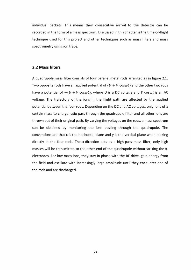
2.2 Mass filters
A quadrupole mass filter consists of four parallel metal rods arranged as in figure 2.1.
Two opposite rods have an applied potential of and the other two rods
have a potential of , where U is a DC voltage and is an AC
voltage. The trajectory of the ions in the flight path are affected by the applied
potential between the four rods. Depending on the DC and AC voltages, only ions of a
certain mass-to-charge ratio pass through the quadrupole filter and all other ions are
thrown out of their original path. By varying the voltages on the rods, a mass spectrum
can be obtained by monitoring the ions passing through the quadrupole. The
conventions are that x is the horizontal plane and y is the vertical plane when looking
directly at the four rods. The x-direction acts as a high-pass mass filter, only high
masses will be transmitted to the other end of the quadrupole without striking the x-
electrodes. For low mass ions, they stay in phase with the RF drive, gain energy from
the field and oscillate with increasingly large amplitude until they encounter one of
the rods and are discharged.

25
Figure 2.1. Example schematic of a quadrupole mass filter [35]
On the other hand, the y-direction acts as a low-pass mass filter where only low
masses will be transmitted to the other end of the quadrupole without striking the y
electrodes. Heavy ions will be unstable because of the defocusing effect of the DC
component, but some lighter ions will be stabilised by the AC component if its
magnitude is such as to correct the trajectory whenever its amplitude tends to
increase. By a suitable choice of RF/DC ratio, the two directions together give a mass
filter which is capable of resolving individual atomic masses [36].
Disadvantages of quadrupole mass filters are:
1. As a ratio of the voltage (U, V) changes, a limit in the resolution is reached
largely determined by the accuracy with which the various quadrupole
parameters are controlled and by the initial motion of the ion as it enters the
quadrupole field. [34]
2. The efficiency of transmission of ions through the quadrupole decreases as ion
mass increases, leading to a relative loss in sensitivity at higher masses.

26
2.3 Mass spectrometry using traps
The quadrupole ion trap uses constant DC and radio frequency (RF) oscillating AC
electric fields to trap ions. The 3D trap consists of two hyperbolic metal electrodes
with their foci facing each other and two hyperbolic ring electrodes halfway between
the other two electrodes. The ions are trapped in the space between these four
electrodes by AC and DC electric fields.
This overlap of a direct potential with an alternative one gives a kind of three-
dimensional quadrupole in which the ions of all masses are trapped on a three-
dimensional trajectory. In quadrupole instruments, the potentials are adjusted so that
only ions with a selected mass go through the rods. In a quadrupole ion trap, ions with
different masses are present together inside the trap and are expelled according to
their masses to create a mass spectrum. The ions repel each other in the trap which
causes an expansion of their trajectories as a function of time. [37]
Figure 2.2. Example schematic of a quadrupole ion trap [38]
To avoid ion loss, the trajectory has to be reduced by maintaining in the trap a
pressure of helium gas that removes excess energy from the ions by collision.
Shown in figure 2.2 is an example schematic of a quadrupole ion trap. Bari et al [39]
used an RF-ion trap combined with a linear time-of-flight mass spectrometer to study
keV ion-induced dissociation of protonated peptides.

27
2.4 Time-of-flight mass spectrometry
The essential principle of time-of-flight mass spectrometry is that ions need to be
extracted from an ion source in short pulses and then directed down an evacuated
straight tube to a detector. The time taken to travel the length of the flight tube
depends on the mass over charge ratio. For singly charged ions, the time taken to
traverse the distance from the source to the detector is proportional to a function of
mass. When the ions reach the detector, a trace of ion abundance against time of
arrival is obtained which is subsequently converted into a mass scale to give the final
mass spectrum. A linear time-of-flight mass spectrometer has two acceleration
regions both containing different electric fields which are used to accelerate the ions
out of the source towards the detector. A reflectron time-of-flight mass spectrometer
uses an einzel lens arrangement to accelerate and focus the ion beam towards a
reflector which provides second order focussing of the beam towards the detector.
For this project a reflectron time-of-flight mass spectrometer (RTOFMS) by R.M.
Jordan Company was used to detect the ions (shown in figure 2.3). The einzel lens
arrangement consists of three electrodes whereby the first and third elements
accelerate the ions and the second electrode focuses the beam (Vfocus in figure 2.3).
The electrostatic field created in the reflector is at the end of the flight path of the
ions and has a polarity the same as that of the ions so they experience a retarding
potential. The voltages applied to Vr1 and Vr2 in figure 2.3 create this retarding field
that acts as an ion mirror by deflecting the ions and sending them back through the
flight tube. The reflectron corrects for a small dispersion in the initial energy of the
ions with the same m/q ratio. The ions with the slightly higher initial kinetic energy will
penetrate the reflectron more deeply and will spend more time in the reflector, thus
they reach the detector at the same time as slower ions of the same m/q.
The ions are detected with a microchannel plate detector (MCP). In our RTOFMS, ions
of adjacent m/q values are separated by about 20 to 30 ns, when they arrive at the
MCP detector. Over a total mass range of 0 - 150 mass units, all of the ions arrive at
the detector over a relatively short time range (typically 62 µs in our instruments).

28
Figure 2.3. Schematic of the reflectron and MCP detector used in this project.

29
The advantages of time-of-flight mass spectrometry are:
1) With typical voltages on the elements of the TOFMS, a complete spectrum can be
obtained every few microseconds (125 µs in our case). This enables the study of how
the relative intensities of different ions vary when source conditions change rapidly.
2) An entire mass spectrum can be recorded for each accelerating pulse, thus it is
possible to measure relative intensities accurately even though source conditions
might vary unpredictably.
3) The accuracy of the TOFMS depends on electronic circuits rather than on extremely
accurate mechanical alignment and on the production of highly uniform, stable
magnetic fields. [40]
The main disadvantage of TOFMS are their limited resolution. Mass resolution is
affected by factors that create a distribution in flight times among ions with the same
m/q ratio. These factors are the length of the ion formation pulse, the size of the
volume where the ions are formed and the variation of the initial kinetic energy of the
ions. Digitizers can also affect the resolution and precision of the time measurements.
One solution to this problem in a linear time-of-flight mass spectrometer is delayed
pulse extraction. To reduce the kinetic energy spread among ions with the same m/q
ratio leaving the source, a delay between ion formation and extraction can be
introduced. In this method, the ions initially are allowed to separate according to their
kinetic energy in the field-free region. For ions of the same m/q ratio, those with more
energy move further towards the detector than the initially less energetic ions. The
extraction pulse applied after a certain delay transmits more energy to the ions that
remained for a longer time in the source. [37]
A better way to improve mass resolution is to use a reflectron time-of-flight mass
spectrometer. In this project, a reflectron and delayed pulse extraction are used to
obtain a good mass resolution and sensitivity. The RTOFMS setup used for this project
will be discussed in more detail in section 3.6.

30
Mass-to-charge ratios are determined by measuring the time that ions take to move
through a field-free region between the source and the detector. The relationship
between m/q and time is discussed below: [41]
The ion TOF in a reflectron can be written as:
(1)
where
and
We define the following quantities independent of m, q:
and
where Ub is the potential in the decelerating gap db; Ur is the potential difference in
the reflecting gap dr. L1 and L2 are the lengths of the drift spaces, qU0 is the mean ion
energy and qU is the ion energy corresponding to the ion velocity components parallel
to the instruments axis.
Inserting quantities A1, A2 and A0 into equation (1) the ion flight time becomes:
(2)
with

31
To allow for the adjustment of the time delay between extraction and the start of the
MCS card, a constant B is added to equation (2) which becomes:
The relationship between m/q and time becomes:
Where
and
This relation is used to calibrate the m/q scale of the mass spectra in section 5.3. This
will allows us to indentify the fragments appearing in our spectrum.

32
CHAPTER 3
Experimental setup
3.1 General overview of the experiment
The main purpose of this chapter is to describe the apparatus used for the research
described in this thesis. The components of the system are discussed individually in
detail under their relevant headings. Detailed below is a general overview of the
experiment.
Figure 3.3. Experimental setup used for this project.
The three chambers (see figure 3.2) are: the expansion chamber where a pulsed
supersonic beam of thymine is generated, the interaction chamber where the clusters
are fragmented using a pulsed electron beam and the reflectron chamber which
33
houses the reflectron time-of-flight mass spectrometer (RTOFMS) where the reaction
products are detected.
Five pumps are used in specific places to keep a suitable vacuum throughout the
system. In the expansion chamber, a diffusion pump coupled with a rotary vane pump
is used to keep the pressure to 7.5x10⁻⁷ mbarr when the oven is in operation. Two
turbomolecular pumps work in tandem with a single rotary vain pump to keep the
vacuum in the interaction chamber and the RTOFMS at a pressure of 1.7x10⁻⁸ mbarr.
The entire vacuum system rests upon an in-house designed and built frame, made
from aluminium. In order to access the instruments inside the vacuum chambers, the
frame has sliding rails which allows the vacuum chamber to be disconnected and
moved apart to access the components in the interior.
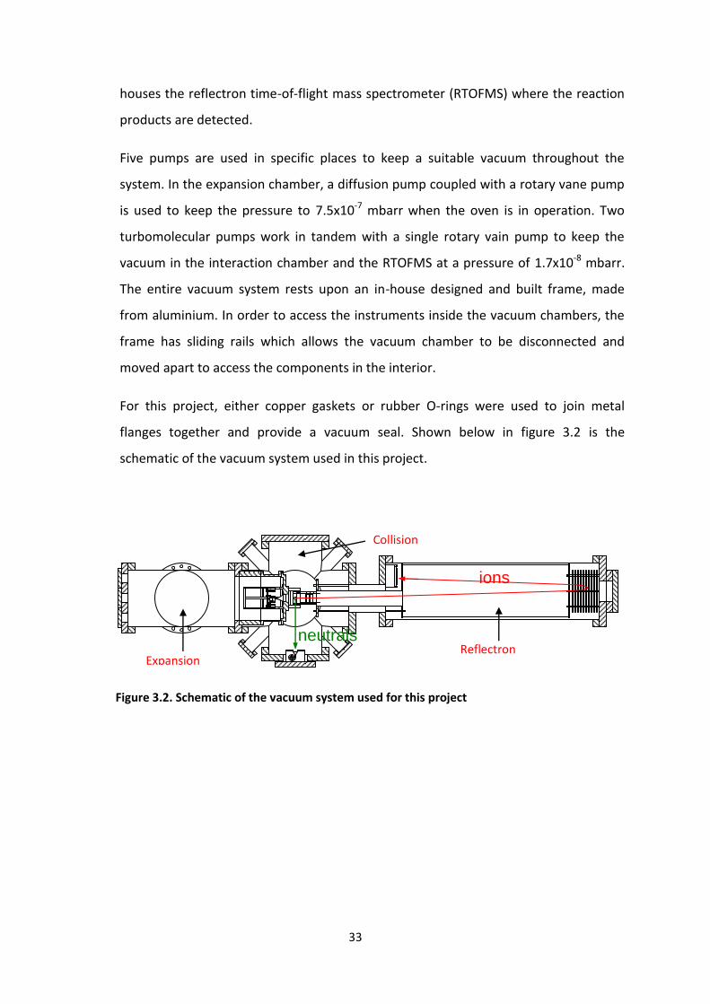
For this project, either copper gaskets or rubber O-rings were used to join metal
flanges together and provide a vacuum seal. Shown below in figure 3.2 is the
schematic of the vacuum system used in this project.
Figure 3.2. Schematic of the vacuum system used for this project
Collision
chamber
Reflectron
chamber Expansion
chamber
ions
neutrals

34
3.2 The expansion chamber
In the expansion chamber a pulsed beam of biomolecules is created using a resistively
heated oven. The chamber is held under vacuum by an Edwards E09K (2800 l/s)
diffusion pump backed by an Alcatel OME 40S rotary vane pump. To separate the
collision chamber from the interaction chamber, an electroplated skimmer with a
diameter of 1.2mm is used. Due to its cone-like shape, this fragile piece of equipment
is preferable to a regular aperture because it easily deflects stray molecules and
creates a forward focused beam of thymine entering the collision chamber. In order to
ensure perfect alignment of the oven and the skimmer, a metal brace was designed
and mounted to the expansion chamber. This metal brace is designed to ensure that
the capillary of the oven will always be aligned to the entrance of the skimmer.
The biomolecular oven is mounted in the center of the expansion chamber and it
houses the nucleobase that is used in the experiment. The oven consists of two parts,
a copper cavity which is heated by a coaxial heating wire that is wound around the
oven and a copper cover that contains an aperture where the thymine exits the oven.
The temperature of the oven is generated by a 0.9 A current which is sent through the
heating wire and is set by the user via an external temperature controller. Once the
current is turned on, a constant stream of thymine is generated at 180 oC. To hold the
oven safely in place, it is mounted on a macor plate which in turn is then attached to a
hollow teflon cylinder designed to fit perfectly into the metal brace. The temperature
inside the oven is measured using a thermocouple that is placed in a small hole in the
copper cavity.
One of the most important aspects of the oven design was its orientation. To ensure
correct alignment, the copper oven is mounted off-center on a macor plate, such that
the capillary which is also off center in the oven is now centered in front of the
skimmer (see figure 3.3). The difficulties of putting the oven pack into the chamber are
reduced significantly thanks to design of the metal brace and the Teflon cylinder. The
oven capillary will always be aligned with the skimmer regardless of how the user
inserts it into the metal brace. Thymine is hydroscopic, so to remove the excess water
content the oven is heated to around 100 oC. Once the pressure in the expansion

35
chamber has dropped to approximately 1 x 10⁻⁷ mbarr, the oven temperature is then
increased to around 180 oC, which allows the thymine to evaporate from the oven.
Shown in figure 3.3 and 3.4 are the schematic of the oven, the skimmer and their
mounting. Figure 3.5 is a picture of oven with thymine in powder form. The coaxial
heating wire around the oven and the oven capillary are also visible.
Figure 3.3. Schematic of the oven and skimmer
A2 A1
Aluminum
Copper
oven
Skimme
r r
Teflon Macor
Skimmer

36
Figure 3.4. Mounting of the oven, skimmer and electron gun on the top hat extending into
the collision chamber. To the right of the electron gun are the einzel lens and deflection
plates which form the entrance to the RTOFMS.
Figure 3.5. The oven with thymine powder. The coaxial heating wire and the oven capillary are visible.

37
3.3 The collision chamber
The second vacuum tank is called the collision chamber. The chamber is held under
pressures of 1.7 x 10⁻⁸ mbarr by a Leybold Turbovac 361 turbomolecular pump backed
by a Trivac D25B rotary vane pump. Here the molecular beam from the expansion
chamber interacts with a beam of electrons that are created using an electron gun.
The electron gun is mounted on a top hat arrangement 90 degrees to the molecular
beam. The area where the molecular beam and the electron beam interact is called
the interaction region. This region is situated between two metal plates A1 and A2
(see figure 3.3). A positive pulsed voltage of 100 V is applied to A1 with a pulsed delay
of 1µs after the pulsing of the electron gun to avoid deflection of the electrons. See
section 4.3 for more details on pulsing.
3.3.1 The electron gun and Faraday cup
The main piece of apparatus inside the collision chamber is the electron gun. This is
used to create a pulsed beam of electrons that interact with the nucleobases, released
out of the oven in the expansion chamber. To release the beam of electrons, a hot
tungsten filament is supplied with a current of approximately 2A. The electrons are
released by thermionic emission from the filament. To accurately focus the beam, four
electrode lens elements called V1, V2, V3 and V6 were incorporated into the electron
gun design. By varying the voltage at each lens, the user can adapt the focus of the
beam. To allow for increased accuracy of the beam, four deflection plates X1, X2, Y1
and Y2 mounted in lens element V3 allow the electron beam to be steered. All lens
elements are made from aluminium and teflon spacers are used to insulate each lens
from each other. All inside surfaces of the lens elements are coated with Aquadag to
help maintain the stability of the electric fields as a function of time.
The gun is also comprised of a grid electrode which is made from stainless steel. The
purpose of this is to set up a weak electric field that suppresses the initial spreading of
the beam being created by the filament. To achieve this, the grid is biased slightly

38
negative with respect to the filament by an external power supply. The gun also has a
filament holder which labelled grid in figure 3.7. The filament is mounted such that the
tip is centered in the hole of the grid element.
To see the collimation of the electron beam, the beam is passed from the gun into the
Faraday cup. The Faraday cup is made up of two separate parts, the inner cup and the
outer cup. The inner cup is held at +40 V and the other cup is held at +10 V. To get a
good collimation of the electron beam, the current must be minimised on the outer
Faraday cup and maximised on the inner Faraday cup. Shown in figure 3.6 is the
electron gun and Faraday cup setup in the Maynooth experiment. Figure 3.7 shows
the schematic of the electron gun and Faraday cup.
Figure 3.6. Electron gun and Faraday cup setup mounted on the top hat. The molecular beam is directed towards the right.

39
Figure 3.7. Schematic of the electron gun and Faraday cup. The molecular beam is directed out of the paper
Outer Faraday cup
Insulating spacer
Inner faraday cup
V6
Filament
V3
V2
V1
Grid

40
3.3.2 Electron gun voltage box
To obtain the desired voltages for the electrode lens elements, an array of potential
dividers is used. The array of potential dividers is contained inside the electron gun
voltage box. For easy adjustment of the voltages, the potentiometers are mounted on
the front panel of the box. The voltages at each element have to be accurately
measured, so voltage test points are on the front panel also. This means the voltages
can be measured using a digital voltmeter while the electron gun is operational. The
voltage box is powered by a Kepco APH 500M power supply (marked 300 V in figure
3.8). This power supply was carefully chosen, because it is a high voltage, low current
dc device with a voltage range of 500V but 300V is typically used and a maximum
current of 40 mA. The voltage box set-up is shown in figure 3.8. As we can see from
the schematic below, the box contains a series of 25 kΩ resistors, 50 kΩ variable
resistors and potentiometers. The resistors were carefully chosen because they
determine the upper and lower values at which the potentiometers can operate. For
the deflection system in the electron gun, the power required is +/-24V DC. This is
provided by two EPSD 15/200C AC-DC converters from VxI Power Limited. The two
convertors provide + 24 and -24 Volts and require 230 V AC input voltage. The incident
electron energy is set with a second Kepco power supply which is used in
programmable mode. This marked as Vincident in figure 3.8.
Figure 3.8. Schematic of the voltage box used to apply voltages to the lens elements of the
electron gun.

41
3.4 The reflectron chamber
The principles of a reflectron time-of-flight mass spectrometer (RTOFMS) are
discussed in section 2.2. The reflectron used in this project was manufactured by R.M.
Jordan Company in California. In the current setup, ions are repelled into the time-of-
flight region by the positive pulsing grid A1 shown in figure 3.3, and are then
accelerated into the einzel lens. The einzel lens is used for focussing of the ions, and
consists of three electrodes whereby the first and third electrodes are held at -1200 V
and the middle one is set to -1400 V.
In order for the ions to reach the detector they must be deflected slightly before
traversing the flight tube. To achieve this, two deflection plates XY1 and XY2 are used
to steer the beam to ensure that ions eventually hit the center of the microchannel
plate detector. XY1 is set to -1200 V and XY2 is set to -1140 V. To provide second order
focussing of the beam, the voltages used in the reflector are VR1 = -390 V and VR2 =
+87 V.
The inside of the RTOFMS has a liner which is kept at a potential of -1200 V. At the end
of their flight path, the ions are detected by a microchannel plate detector (MCP)
which is operated at -3800 V. This voltage is divided across a voltage divider network
in the MCP detector resulting in VD1 = -1672 V, VD2 = -912 V and VD3 = -180 V. Where
VD1 is applied to the front of the first plate, VD2 is applied to the back of the first plate
and also to the front of the second plate, and VD3 to the back of the second plate (see
figure 3.9). This is to ensure the voltage never exceeds 1000 V across any of the plates.
Both plates in the MCP detector are mounted in a chevron arrangement. Shown in
figure 3.10 is the MCP detector used in the reflectron chamber to detect the ions.
Figure 2.3 in the previous section shows the schematic for the reflectron and MCP
detector used in this project.

42
Figure 3.9. Schematic of the MCP detector used in this experiment
Figure 3.10. The MCP detector used in the reflectron chamber to detect the ions
Anode= 0V
VD3= -152 V
VD2= -912 V
VD1= -1672 V

43
3.5 The interlock system
To ensure the safety of the entire vacuum apparatus, an interlock box is used. This is
an integral part in the project because, in the event of a power failure or a equipment
malfunction the entire vacuum system including all electronics needs to shut down
and not restart. This is extremely important because if the system would restart after
a power failure, only the oil sealed rotary vain pumps and the diffusion pump would
turn back on. This could cause the pumps to evaporate oil in to the chamber and
damage the equipment. To prevent this from happening, all the main equipment and
electronics needed for the vacuum system has to be interlocked with each other.
The interlock box incorporates six external trip switches. Each switch can be bypased
by toggle switches on the front panel of the interlock box. In order for the interlock
box to work effectively, sensors were placed in specific areas of the vaccuum system.
While the system is interlocked, if one of the sensors detects a problem, the entire
system will shut down and not restart. This process is due to the solid state relay
devices inside the box which act as electronic switches. It is because of this, that the
experiment can run for very long periods of time without the need for constant
observation. The flow of cold water from the chiller into the diffusion pump needs to
monitored so, a sensor is placed there. The temperature of the diffusion pump is also
monitored with a sensor. To prevent the system pressure from going above a certain
level which is set by the user, trip switches were also set on the ion gauges. Trip
switches were also used for the two turbopump controllers to ensure the pumps stay
off. Monitoring the safety of the turbopumps is extremely important because, in an
emergency situation a backdraft of air could cause damage to the blades of the
pumps.
When evacuating the system after a restart, all the over-rides must be activated and
the start/restart push button pressed. Then, as the pressure, cooling and temperature
trip points are safely crossed, the green LED is lit for each trip. When this happens
each trip may be safely interlocked by switching the toggle switch from the over-ride
into the interlocked position.

44
CHAPTER 4
Interfacing, data acquisition and data analysis software
4.1 Introduction
This chapter describes the procedures followed to acquire a mass spectrum as a
function of electron impact energy and to calibrate the electron gun. The interfacing
hardware and the programs needed for data acquisition are described. The main
instrument for data acquisition is a FAST ComTEC multichannel scaler which is
described in detail in section 4.4. In this experiment, timing is of the utmost
importance for the generation and acquisition of the data in this experiment. To
acquire a mass spectrum a 3 step sequence needs to occur. Immediately after the
electron gun is pulsed, the pulsing of the extraction voltage is used to extract the ions
out of interaction region, and multichannel scaler (MCS) is triggered. The pulsing and
timing sequence of the various elements of the system are set via a digital delay
generator described in section 4.2. The operation and calibration of the MCS is
described in section 4.3 and the data acquisition and hardware programs used to
operate various hardware devices and to record the data from the time-of-flight scans
are described in section 4.5.
All of the data acquisition programs are designed in LabVIEW. LabVIEW is a graphical
programming language from National Instruments that can be used for the acquisition
and recording of data, the control of external electronic devices, and data analysis.
LabVIEW is a type of dataflow programming where writing a program requires
selecting relevant icons, placing them on a block diagram and wiring them together.
There are two panels in each program, the front panel contains the user interface

45
which displays all the relevant input and output data to the user such as controls,
graphs and indicators. The second panel is called the block diagram where all the
graphical code is written and sent to the front panel. LabVIEW differs from text based
coding because the event execution is not in order and the data is passed to the user
when it becomes available. The programs used to operate and analyse various parts of
this project are explained in detail in section 4.5.
4.2 Amplifier and timing discriminator
When an ion is detected by the microchannel plate detector (MCP) the signal
produced must be amplified and discriminated before the data acquisition can occur
at the MCS card. The signal from the MCP passes into an ORTEC 9327 1GHz amplifier
and timing discriminator. The 9327 is optimized for use with millivolt signals produced
by multichannel plate detectors. The amplifier provides a 1 GHz bandwidth to
minimise the noise and rise time contributions to timing jitter on detector pulses
having widths as narrow as 250 ps FWHM.
The device is designed to handle pulses in the range of 0 to -30 mV. An oscilloscope is
not needed to adjust the gain because the device contains an over-range LED that
indicates when the pulse amplitudes have exceeded the full-scale limit of the
amplifier. To eliminate the noise from the signal, the 9372 contains a discriminator
with a discriminator level that is manually adjusted at the front of the device. The
detection of a pulse is indicated by a flash of the output LED, however, this could not
be used in this experiment because of the noise generated by the pulsing of the ion
extraction and the electron gun. Instead the discriminator level was set by taking
single mass spectra and monitoring the background signal between the mass peaks.
The noise produced by the pulsing of the ion extraction and the electron gun produces
a large amount of spurious counts in the first few bins when the B pulse for the DG535
digital delay generator (see next section) is used as the start pulse of the MCS. For this
reason, an ORTEC 416A Gate and Delay Generator was used to delay the B pulse by 1
µs.

46
4.3 Pulsing and timing
For this project the electron pulse, ion extraction pulse and the trigger for the MCS are
created using a DG535 digital delay generator designed by Stanford Research Systems
Inc. This is an extremely important device for the project because the electron pulse,
ions extraction pulse and the MCS trigger all require the correct width and delay with
respect to each other in order for the experimental setup to operate correctly. The
DG535 is a very precise delay and pulse generator that provides four precision delays
outputs (A, B, C and D) and two independent pulses (AB and CD) with 5 picosecond
resolution. Trigger to output jitter is less than 50 picoseconds. Each delay can be set
from 0 to 1000 seconds relative to the trigger with 5 picosecond resolution. The two
pulse outputs AB and CD and their inverses are defined as pairs of delay outputs. The
first delay specifies the leading edge of the pulse, while the second delay defines the
trailing edge or pulse width. The pulse shapes can be TTL, ECL, NIM or VAR and the
pulse out can be normal or inverted with an impedance of either 50 Ω or high.
Figure 4.1. Timing cycle of the DG535 digital delay generator [42]

47
The T0 pulse marks the beginning of a timing cycle and is generated by either the
internal rate generator or in response to an external trigger. This output is asserted
approximately 85 ns following the trigger. The other outputs A, B, C and D are
asserted relative to T0 after their programmed delays. All of the delay outputs return
low about 800 ns after the last delay is asserted. The pulse outputs AB and CD go high
for the time interval between their corresponding delay channels. [1]
The delays settings used in this project for outputs A, B, C, and D are shown below in
table 4.1. For the thymine measurements in this report the repetition rate used was 8
kHz (125 µs between successive pulses) and the time-of-flight range was 62 µs.
A = T0
B = D + 1 µs
C = A + 1 µs
D = C+ 0.8 µs
Table 4.1. Delay settings used in this project for ouputs A, B, C and D
Figure 4.2. Pulse settings used in this project for ouputs AB, CD, Output electron pulse and the Output extraction pulse
+100
V
- Vinc - 30 V
-Vinc
CD
0.25
0.25
1.25
0.55 1.0
1.
0
0.8 1.
0
AB
Output electron
pulse
Output extraction pulse
0 V

48
Two remote pulsers are used to control the electron pulse and the extraction pulse of
the electron gun. Each pulser is connected directly to the appropriate vacuum-
feedthrough, and requires 12 V to power its circuit, two dc voltages which specify the
low and high voltages of the output pulse, and a TTL trigger pulse which determines
the timing of the output pulse. Figure 4.2 shows that both remote pulses have delays
between the TTL trigger pulse and the output pulse they provide. The pulse settings
used for the remote pulsers are shown in figure 4.2. The AB pulse from the digital
delay generator is used to trigger the remote pulser for the ion extraction voltage on
the grid. The voltage on the extraction grid must be dropped to ground from +100 V.
The CD pulse is used to trigger the remote pulser for the electron gun which pulses
from –Vinc -30 V to –Vinc.

49
4.4 Multichannel Scaler card
The data acquisition for this project is carried out by the 7886S Multichannel scaler
card by FAST ComTEC. The card is capable of accepting one event in every channel and
can handle up to 2 GHz of peak count rates. It has a dynamic range of up to 237
channels, which enables sweeps for 68.7 seconds with a time resolution of about 500
ps per channel (430 ps for our MCS). [43]
The card is controlled using a server program that contains a set of functions stored in
a dynamics link library (DLL). Two of the parameters that can be controlled by the
server program are the bin width and the time range. The bin width can be chosen in
powers of 2 up to 16,384 channels (each with a dwell time of 430 ps). The range is the
length of the spectrum in bins. Most of the thymine mass spectra were recorded with
a binwidth of 128 channels (55.0 ns) and a range of 1122 bins (61.8 µs). The user
interface software provided by FAST ComTEC is called MCDWIN and this allows the
user to control the server settings and display the data in real time. For this project,
the MCDWIN user interface has been replaced by LabVIEW programs which provide a
more flexible user interface. The LabVIEW programs that interact with the MCS card
are described in section 4.5. The MCS card contains a number inputs and outputs:
STOP IN, START IN, ABORT IN, SYNC OUT, DIGITAL IN and a THRESHOLD ADJUST screw.
Output B of the digital delay generator is delayed by 1 µs and connected to the START
IN input and this triggers a sweep of the MCS card. The multichannel plate detector
output is connected to the input of the ORTEC 9327. The NIM OUT output of the
ORTEC 9327 is connected to the STOP IN of the MCS card , so that the signal from the
detector is registered as a count at the relevant binning location of the MCS.
The MCS card utilizes a phase-locked loop (PLL) oscillator that is set to at least 1.8 GHz
which results in an assured time resolution of less than 500 ps per channel. This
frequency can vary so the time per channel must be calibrated using an external

50
reference. To calibrate the MCS card, the DG535 digital delay generator is used to
send a start and stop pulse to the MCS card. The DG535 digital delay generator
provides four precisely timed outputs, which can be set with a precision of 5 ps and
have a low jitter (50 ps). The LabVIEW program getspectrum-3-5.vi described in
section 4.5.2 was used for the calibration. The delay in the pulses was varied over 55
µs in steps of 5 µs and then plotted against the corresponding bin number as shown in
figure 4.3 below. As in previous calibrations a binwidth of 32 channels was used.
Figure 4.3. Graph to calibrate the MCS card. The delay in the pulses was varied over 55 µs in steps of 5 µs and then plotted against the corresponding bin number.
The best fit line was drawn through these points and the slope was found to be 0.0727
± 0.0047 bins per ns, yielding a dwell time of 430.0498 ± 0.0020 ps per channel. This is
in good agreement with a previous experiment by Jason Howard [44]. For the
measurements on thymine a bin width of 128 channels was used, corresponding to
55.04638 ± 0.00026 ns per bin.
y = 0.0727x + 1.3291 R² = 1
0
500
1000
1500
2000
2500
3000
3500
4000
4500
0 10000 20000 30000 40000 50000 60000
bin
s
Delay (ns)

51
4.5 LabVIEW programs
4.5.1 Testing the electron gun
Two previously developed LabVIEW programs are used to set the electron impact
energy (Vincident in figure 3.8) and to test whether the electron gun produces a beam
with a constant current as the electron energy is varied.
A KEPCO APH 500m power supply is used to set the electron impact energy. This is a
high voltage 0-500 V, low current and precision-stabilised d-c source. It has an
automatic crossover between voltage and current stabilisation mode of operation
with visual front panel LED mode indicators. The power supply also has programming
terminals on the back panel which are connected to a NI myDAQ data acquisition
device.
NI myDAQ is a low-cost portable data acquisition (DAQ) device manufactured by
National Instruments that uses NI LabVIEW-based software instruments. There are
two analog input channels on NI myDAQ. These channels can be configured either as
general-purpose high-impedance differential voltage input or audio input. The device
also contains two analog output channels. These channels can be configured as either
general-purpose voltage output or audio output. Both channels have a dedicated
digital-to-analog converter (DAC), so they can update simultaneously.
To test the KEPCO power supply, a LabView program called set-gun-V-myDAQ.vi is
used. To control the APH output voltage between 0-500 V, a control potential from 0-
5 V must be applied to the input of the main voltage amplifier. The myDAQ can
provide a ±10 V but it is important that the applied voltage to the Kepco power supply
does not rise above 5 V ± 2%. To ensure this, a limiting function is used in the LabVIEW
code to ensure the voltage does not go over 5 V. The code divides the incident voltage
by 100 and displays the output voltage on the front panel. A LED indicator is also on
the front panel to tell the user if the incident voltage is in range.
52
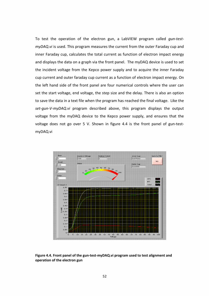
To test the operation of the electron gun, a LabVIEW program called gun-test-
myDAQ.vi is used. This program measures the current from the outer Faraday cup and
inner Faraday cup, calculates the total current as function of electron impact energy
and displays the data on a graph via the front panel. The myDAQ device is used to set
the incident voltage from the Kepco power supply and to acquire the inner Faraday
cup current and outer faraday cup current as a function of electron impact energy. On
the left hand side of the front panel are four numerical controls where the user can
set the start voltage, end voltage, the step size and the delay. There is also an option
to save the data in a text file when the program has reached the final voltage. Like the
set-gun-V-myDAQ.vi program described above, this program displays the output
voltage from the myDAQ device to the Kepco power supply, and ensures that the
voltage does not go over 5 V. Shown in figure 4.4 is the front panel of gun-test-
myDAQ.vi
Figure 4.4. Front panel of the gun-test-myDAQ.vi program used to test alignment and operation of the electron gun

53
4.5.2 Acquiring single mass spectra
For the acquisition of single scans of mass spectra, a program called getspectrum-3-
5.vi is used. The primary use of this program is to acquire a single mass spectrum
before doing multiple time-of-flight scans (described in next section). The program
records data from the MCS and allows real-time observation of data while it is being
acquired and displayed on the graph. In order for LabVIEW to interact with the MCS
card, a dynamic link library file (DLL) is needed. For this project, the DLL files were
provided by Dr. Marcin Gradziel and are a modified version of the code provided by
FAST ComTEC. The DLL files contain C code written for communication with the MCS
card and these files are accessed in LabView via the use of the Call Library Function
nodes. See appendix for the C code used in the DLL files.
In this program, two different nodes are used. Both DLL’s use the same C code but,
they access different functions within the code itself. The first node initialises the MCS
card and the second one deals with the measurement of the data. The three inputs
that the second node reads in are variables time range, update timeout and nr of
sweeps which are determined by the user on the front panel. One of the outputs is an
array that is initially empty and is added upon with each sweep of the MCS and a
complete time of flight spectrum is formed when all the sweeps have been completed.
The second output is called completed sweeps, which shows the actual number of
sweeps the card performed. Before running a scan, the user must decide on the
correct time range and bin width by using the corresponding numerical controls on
the front panel. Once the user starts the program, it can be stopped at any point and
resumed using the continue push button. The save button is used to save the
completed spectrum as a text file for further analysis. This program also displays the
current state of the MCS card on the front panel so the user can make sure that the
MCS card is operating correctly. The control structure used in this program is a
standard state machine. The standard state machine is a case structure contained
within a while loop. Execution of particular cases in the structure is determined by the
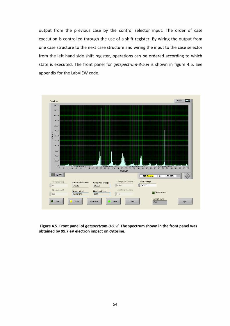
54
output from the previous case by the control selector input. The order of case
execution is controlled through the use of a shift register. By wiring the output from
one case structure to the next case structure and wiring the input to the case selector
from the left hand side shift register, operations can be ordered according to which
state is executed. The front panel for getspectrum-3-5.vi is shown in figure 4.5. See
appendix for the LabVIEW code.
Figure 4.5. Front panel of getspectrum-3-5.vi. The spectrum shown in the front panel was obtained by 99.7 eV electron impact on cytosine.

55
4.5.3 Acquiring multiple mass spectra
Spectra-vs-E-v7.vi is the main program used in the acquisition of mass spectra as a
function of electron impact energy. This LabVIEW program was developed from a
preliminary version coded by Gerard Barrett [45], and also uses the DLL files provided
by Dr. Marcin Gradziel (see previous section). This program takes mass spectra
sequentially with the electron energy incremented by a step size over a certain range
of electron energies. Like the program in the previous section, Spectra-vs-E-v7.vi gives
the user complete control over the MCS settings via the front panel such as: the range
or number of channels (Time range), the number of sweeps per scan (nr of sweeps),
and the number of bins per channel (Bin width). The user also has control over the
number of cycles, the starting and stopping impact energy and the step size. A cycle is
a loop of scans through a certain range of electron impact energy. After the impact
energy is increased there is a time delay (Stabilisation) to allow the electron gun to
stabilise.
After completion of each cycle, the full 2 dimensional array of accumulated mass
spectra as a function of electron energy is written to a file with a name specified by
the user and with the cycle number appended to it. This means that after completion
of an entire measurement comprising of a number of cycles, the yield of a specific
mass at a specific electron energy can be inspected as a function of cycle number, to
see whether there was any depletion in the intensity of the thymine beam while the
measurements were in progress.
The front panel is shown in figure 4.6 with all the inputs and outputs on display. The
user has three options to abort the accumulation of the data. They are finish current
cycle, finish current energy or abort TOF accumulation. Choosing the abort TOF
accumulation will the program instantly whereas the other two options will wait until
the current cycle or energy is finished. The front panel of the program displays each
mass spectra being accumulated, and the current cycle number (Cycle), sweep
number (sweeps completed), step number (E nr). The four green LED lights above the
graph indicate the current state of MCS.

56
Figure 4.6. Front panel of Spectra-vs-E-v7.vi. The spectra shown is for 58 eV electron impact on cytosine.

57
4.5.4 Gaussian Peak fitting
To obtain an accurate peak area for all the fragments over a range of 0-99.7 eV, a
program called multigauss test.vi was created as part of this project. This is an
important program for this project because an accurate determination of the peak
area of each peak mass is needed for the creation of excitation functions. To fit a
series of adjacent mass peaks, the Levenberg-Marquardt algorithm vi is used in the
program. The Levenberg-Marquardt algorithm determines the set of parameters that
best fit the set of input data points (x, y) as expressed by a nonlinear function y =
f(x,a), where a is the set of parameters.
The algorithm needs a model function. For this project, each sequence of adjacent
peaks was fit using a sequence of normalised Gaussian functions given by:
where C is peak area, pi is position of peak i, a is the peak width (assumed equal for
the adjacent peaks) and b is the background.
To insert the Gaussian function into the LabVIEW program, a model string was used.
This string allows the user to describe the model equation, define parameters and edit
the equation to suit the fit of the data. The model string used for the fitting is shown
in figure 4.7. Here the Gaussian function is repeated six times for the peaks c1-c6 and
the peak position p and peak width a are determined by the user on the front panel.
Depending on the fit results, p and a can be either variable or fixed. To ensure the
area under the curve is 1, a normalisation factor of
was inserted into the model
string. The input data for this program is extracted from the output file of the Spectra-
vs-E-v7.vi program. The user decides on the bin range to be fitted, copies that range
from the output file of the Spectra-vs-E-v7.vi program and saves the data as a text file.
This program fits the data with bin range on the x-axis and counts collected on the y-
axis.
ba
px
a
Cxf i
n
i
i
2
1
exp)(

58
In order to avoid problems with conversion of the fitting while stepping through the
data as a function of electron impact, a number of precautions had to be taken.
Separate vi's were made for each group of peaks extracted from the full data set. In
each vi the model string was changed accordingly. Figure 4.7 shows the model string
for the 51 u to 56 u peaks of thymine. It is assumed that the width a of all peaks are
the same, and that the distances between the peaks are constant. The numbers
contained in the model string in figure 4.7 show the distances from the 55 u peak (at
position p) in units of bins, obtained from the mass calibration described in section
5.3. Based on inspection of the mass spectra, the background was set to 1.
While fitting groups of peaks with decreasing electron energy, it was found in a
number of cases that for low energy the fits would not converge any more. In these
cases the number of peaks would be reduced if possible, and the width a would be
fixed to the average value obtained at higher electron energies.
Figure 4.7. Model string containing the set of normalised gaussians used to fit the 51 u to 56 u peaks of thymine.

59
The front panel of multigauss test.vi is shown below in figure 4.8. The initial
parameters array is where the user must input the estimates for the area of each
peak, the position of the peak with the highest mass and the peak width. The size of
the array will change depending on the number of peaks to be fitted and if a and p are
made constant in the formula string. The best fit parameters array displays the best fit
values obtained at each energy, which is then subseqentially stored in an array that
contains all the best fit parameters when the program completes the 200 fits. In this
project we used 200 fits because we used an energy range of 0-99.7 eV in steps of 0.5
eV. The load push button is used to load the text file containing the peak data into the
program. The user can then choose how many rows of data to fit via the Data Entry
Limits: Maximum and the Data Entry Limits: Minimum numerical control. If the user
wants to fit the peaks in the 80-99.7 eV range, the maximum value would be 200 and
the minimum value would be 160 because our mass spectra was created with 5 eV
steps. The program will then load the full text file and only choose the data between
the minimum and maximum values.
A time delay was inserted into the front panel in order to slow the fit process so that
the fitting process can be inspected. This is an important addition because the
program will sometimes fail to fit the peaks at low energies, so slowing the program
down to see when this occurs will help decide on the minimum and maximum limits
for that data set. The three output arrays, bin number, contents and error at the top
of the front panel are used for error checking the data set that needs to be fitted.
Shown in table 4.2 are the mass ranges that were fitted using this program and the
corresponding bin and the time range for each of the mass groups.

60
Figure 4.8. Front panel of multigauss test.vi. The spectrum shows a fit of the 51-56 u peaks of thymine at 90 eV.
u range bin range TOF range (us)
16 - 18 335 - 370 18.440 - 20.147
25 - 29 428 - 465 23.559 - 25.376
35 - 46 515 - 583 28.348 - 32.092
51 - 56 613 - 665 33.743 - 36.606
70 - 71 720 - 735 39.633 - 40.459
82 - 84 781 - 798 42.991 - 43.927
97 845 - 862 46.514 - 47.450
124 - 127 963 - 985 53.009 - 54.220
Table 4.2. The thymine mass ranges that were fitted using this program and their
corresponding bin and time range

61
CHAPTER 5
Test measurements with thymine
The purpose of this chapter is to present the various test that were conducted when
thymine was in the oven, including the calibration of the electron gun and the mass
spectra. An analysis of the water peaks used to convert the incident voltage scale to
incident energy scale is also included. During measurements it was found that the
intensity of the thymine beam was depleted, and this is also discussed in this chapter.
5.1 Comparison of LabVIEW programs to MCS
To ensure the LabVIEW programs were not missing counts coming from the
microchannel plate detector, two tests were carried out with the multichannel scaler
card. In the first test the MCDWIN program used to control the MCS card is compared
to the LabVIEW program getspectrum3.5.vi. Both programs are described in depth in
section 4.3 and 4.5. The parameters of the MCDWIN program card were: range of
1024 bins, 4,302,156 sweeps and a bin width of 128. The getspectrum3.5.vi
parameters were: range of 1122 bins, 5,000,000 sweeps and a bin width of 128. An
Excel plot was created from the resulting data files and is shown in figure 5.1. The
LabVIEW data points compare well with those of MCDWIN and, only a small
multiplication factor (i.e. ratio of number of sweeps) is needed to align the data points
in MCDWIN with the LabVIEW data. For the second test, the getspectrum3.5.vi
program was used twice with adenine instead of thymine, at a pulse rate of 8 kHz and
400 Hz with 720,000 sweeps. The resulting graph is shown in figure 5.2 and both mass
spectra are in excellent agreement.

62
Figure 5.1. Test of MCDWIN and getspectrum3.5.vi with thymine
Figure 5.2. Test of getspectrum3.5.vi with adenine
1
10
100
1000
10000
100000
0 10 20 30 40 50 60 70 80 90 100 110 120 130 140 150 160
MCDWIN
Labview
1
10
100
1000
10000
0 10 20 30 40 50 60 70 80 90 100 110 120 130 140 150 160
8000 Hz
400 Hz

63
5.2 Calibration of Electron Gun
An important test to undertake before taking experimental measurements of
excitation functions is to make sure the electron gun has a constant current when the
electron energy is changed. To test the electron gun, two LabVIEW programs are
used. The first program is set-gun-V-mydaq.vi and the purpose of this is to set the
acceleration voltage and electron energy of the gun. The second program is called
gun-test-mydaq.vi, both of these programs are described in detail in section 4.5.
Figure 5.3 shows the optimum setting for the electron gun which was found using the
gun-test-mydaq.vi program.
Figure 5.3. Optimum setting for the pulsed electron gun.
Table 5.1 below shows the optimum voltage and current settings for the pulsed
electron gun used to take the experimental measurements for this project. The
incident voltage scale (Vinc) has been converted to incident energy (eV) using the
calibration method described in section 5.4. As we can see from the above graph, the
electron gun shows constant current down as far as approximately 16 eV after which
the current begins to deteriorate. At 9 eV we still get an estimated 60% of current
which means we should clearly see the onset of the thymine parent ion peak (126 u)
at 8.8 eV. The IFC current was 1.385 µA and the OFC current was 0.026 µA at 99.7 eV.
0
0.2
0.4
0.6
0.8
1
1.2
1.4
1.6
0 10 20 30 40 50 60 70 80 90 100
Cu
rre
nt
(µA
)
Incident energy (eV)
OFC
IFC
Total

64
Setting V (pulsed)
V filament 3.01
I filament 2.246
V Grid -0.0064
V1 46.1
V2 290.6
V3 84.3
V x1/x2 -4.60/4.60
V y1/y2 -10.9/10.9
V6 12.4
Table 5.1. Current and voltage settings used for the electron gun

65
5.3 Calibration of Mass Spectra
In order to calibrate the mass spectrum for correct analyses, the time of flight scale
must first be converted to mass per charge ratio (m/q). To convert the scale we must
first find the constants of calibration C and D using the following formula which is
described in chapter 2.
(1)
Figure 5.4 shows the thymine mass spectrum at 70 eV with the time scale on the x-
axis. Eight prominent peaks in the spectrum were chosen, the square root of their
mass was plot against the corresponding time and a straight line was fit to the data as
shown in figure 5.5. The value for C was calculated to be 0.206677 ± 0.000027 and D
was found to be 0.1388 ± 0.0011.
Figure 5.4. Thymine mass spectra at 70 eV with a time of flight scales on the x-axis
0
5000
10000
15000
20000
25000
0 10 20 30 40 50 60
rela
tive
inte
nsi
ty
time (us)
x 0.25

66
Figure 5.5. Plot to find the calibration constants C and D
The time scale was converted to mass/charge by using (1) and the constants of
calibration C and D. A plot of m/q versus relative intensity is shown in figure 5.6. For a
detailed discussion on which fragments are visible, refer to section 1.5.
Figure 5.6. Thymine mass spectra at 70 eV with m/q on the x-axis
y = 0.2067x + 0.1388
0
2
4
6
8
10
12
10 20 30 40 50 60
sqrt
(m
/q)
time (us)
0
5000
10000
15000
20000
25000
0 10 20 30 40 50 60 70 80 90 100 110 120 130 140 150
rela
tive
inte
nsi
ty
m/q (u)
x 0.25

67
5.4 Analysis of water peaks
For the study of the water peaks obtained in this project, the data presented in the
review paper by Y. Itikawa and N. Mason [46] is used for comparison. This paper
contains a compilation of all the major cross section data for electron collisions with
water molecules. For the ionization cross section of the water molecules, this paper
provides the relevant data from Straub et al [47] who used a parallel plate apparatus
with a time of flight mass spectrometer to obtain the data. The data obtained by
Straub et al has been slightly corrected by Lindsay and Mangan [48] due to a
recalibration of their apparatus.
The excitation functions for the 16 u, 17 u and 18 u water peaks were determined
using the peak fitting routine described in section 4.5.4. For each excitation function
the onset was determined by drawing a straight line segment through the linear
portion of the rising part of the excitation function. Table 5.2 shows the observed
onset voltage found for the water peaks compared to onset energy of Itikawa and
Mason. The onset voltage here refers to the voltage of the Kepco power supply which
determines the electron impact energy (see section 3.3.2).
Observed onset (V) Onset I & M (eV)
18 u 16.1 12.621 ± 0.002
17 u 21.6 18.116 ± 0.003
16 u (21.0) 19 ± 0.2
Table 5.2. Observed onsets for water peaks compared to Itikawa and Mason [46]
This data indicates that in our experiment the incident electron energy is related to
the voltage by Ei = Vi – 3.5 , where Ei is incident energy, Vi is the incident voltage of the
band 18 u onsets and the data from Itikawa and Mason. (The 16 u onset deviates
somewhat, see discussion below).

68
Figure 5.7. Excitation functions of 17 u and 18 u compared to Itikawa & Mason [46]
Figure 5.8. Excitation functions for 17 u and 18 u in the range of 10-40 eV.
0
50
100
150
10 20 30 40 50 60 70 80 90 100
Ion
ye
ild (
cou
nts
)
Incident energy (eV)
Maynooth 17 u
Maynooth 18 u
Itikawa & Mason 17 u
Itikawa & Mason 18 u
0
50
100
10 20 30 40
Ion
yie
ld (
cou
nts
)
Incident energy (eV)
Maynooth 17 u
Maynooth 18 u
Itikawa & Mason 17 u
Itikawa & Mason 18 u

69
When this energy calibration was applied to the measured excitation functions, it was
found that the shift of 3.5 V was slightly too high, and that a better agreement was
obtained by reducing the shift to 3.1 V. The excitation functions obtained using this
energy calibration for the horizontal scale are shown in figures 5.7 and 5.8. Both
graphs compare the excitation functions for 18 u (H20+) and 17 u (OH+) to the data
from Itikawa and Mason. Our experimental data was normalised to the cross sections
of Itikawa and Mason at 30 eV.
The 16 u excitation function compares less well with the Itikawa & Mason data and is
not shown here. This could be due to contribution from the 16 u fragment of thymine.
For this reason, and also because of the 16 u onset from Itikawa & Mason has the
largest uncertainty, the average of the differences of our 17 and 18 u onsets with the
Itikawa & Mason was taken as the calibration.
The residual water in the Maynooth apparatus could come from two sources in the
experiment. If the water is coming from the expansion chamber, the skimmer will
prevent the majority of the water molecules from entering the collisions chamber. The
most probable explanation is that the water is coming from the walls of the collision
chamber so that the water ions will be generated over the entire section between the
electron gun and the Faraday cup.
Another possible source of water is the thymine in the oven. Thymine is hydroscopic
so there could be water contained in the thymine powder that is released when the
oven is heated. This contribution is assumed to be small because no significant
depletion was observed in the water peaks while the thymine was depleting (see
further discussion in section 5.5.2), and there was no great variation in yield when the
oven temperature was increased (see next section).

70
Assuming that the water is mostly coming from the walls of the vacuum chamber, 16
u, 17 u and 18 u ions would be generated in the section of the electron beam between
the exit of the electron gun and the entrance to the Faraday cup. Ions passing through
the aperture A2 (see figure 3.3) will enter the RTOFMS, but ions passing near the edge
of the aperture may not hit the MCP detector, which could be the reason for the small
deviation of the excitation functions from the published cross sections in figure 5.7.

71
5.5 Oven Tests
5.5.1 Oven temperature
Using the getspectrum3.5.vi program described in chapter 4, a test was conducted to
verify the temperature needed to generate a steady stream of thymine from the oven.
A current of 0.9 A was used to increase the oven temperature to a maximum of 180
oC. While the oven temperature was increasing, a series of mass spectra were
obtained at regular intervals. For each mass spectra shown, the temperature
increased by about 2.5 oC during accumulation until 180 oC was reached.
The water peaks are somewhat higher than anticipated. There is a presence of the
water peaks at lower temperatures and a lack of depletion as the temperature is
increased shows that they are largely due to the background. The expansion chamber
was heated to about 80 oC but this did not improve the situation. Heating of the entire
vacuum chamber will be implemented in the near future. It is not expected that the
presence of water in the vacuum system has had any effect on the mass spectra
obtained with thymine. There is no indication of any signal at 144 u due to thymine
with a single water molecule attached. Every time after refilling the oven, all efforts
were made to ensure the walls of the expansion chamber were clean before closing
the chamber by using clean tissues and methanol.
A small amount of remnant air is present in the chamber as is indicated by 32 u peak
which is not a thymine fragment (see section 6.1). At 160 oC, all the main groups of
peaks are present including the thymine parent ion at 126u. In the 180 oC spectrum, all
of the peaks are at their highest intensity and a steady stream of thymine is now
available. For the duration of the project, the oven was set to 180 oC. It is noted that
the 35 u, 36 u and 38 u peaks are significantly higher for 140 oC. We are not sure why
this is, however our mass spectrum taken at 180 oC is in good agreement with other
measurements, see figure 6.1 in section 6.2.

72
Figure 5.9. Appearance of thymine from the oven as the temperature is increased (at 99.7
eV).
In initial tests, the oven was heated to 100 oC for one or two days but it was realised
that this did not reduce the background peaks in the spectra. This also shortened the
time over which the thymine beam depleted (see next section). The measurements
presented in this report were taken without pre-heating the oven to 100 oC and
without heating the expansion chamber.
5.5.2 Oven Depletion
In all measurements on thymine done during the course of this project, it was
observed that the intensity of the thymine beam depleted in the course of 6 to 16
hours, even though there was enough thymine left in the oven. There was no
indication of blockage of the oven capillary. This depletion was not observed in
measurements with other nucleobases.
A test was conducted to see if the oven depletion had an effect on the full spectrum
over a range of cycles. For this test, cycle 1, 9 and 17 were chosen and plot of relative
intensity versus m/q was created and is shown in figure 5.10. For increased accuracy,
0
200
400
600
800
1000
1200
1400
1600
0 10 20 30 40 50 60 70 80 90 100 110 120 130 140
Re
lati
ve y
ield
(co
un
ts)
m/q (u)
31.6 C
140 C
160 C
180 C
x 0.25

73
the relative intensity axis was set to logarithmic scale and we can see that cycle 1, 9
and 17 have excellent agreement with each other.
Figure 5.10. Depletion test for cycles 1, 9 and 17
The data that is being analysed in this project was taken over 24 cycles. The signal
accumulated after completion of cycle 14 is used for analyses in chapter 6. During the
final cycles it became apparent that the source was starting to deplete and it
eventually depleted entirely during cycle 24.
A correction factor was developed to correct for the depletion in the data. To create
the correction factor it is assumed that the total source density is given by:
(2)
where s = initial source density, d = depletion of source density over 1 cycle and t =
time and T = duration of one cycle
From eq. (2) table 5.3 was created, containing the source density at the start, end and
the cumulative signal at the start and end of cycle 1 to n. From the fit data in Excel we
obtain d= 253.62 and s = 7096.0.
10
100
1000
10000
0 10 20 30 40 50 60 70 80 90 100 110 120 130 140
Re
lati
ve y
ield
(co
utn
s)
m/q (u)
Cycle 1
Cycle 9
Cycle 17

74
source density cumulative signal
cycle at start at end at start at end
1 s s-d s s-d
2 s-d s-2d 2s-d 2s-3d
3 s-2d s-3d 3s-3d 3s-6d
4 s-3d s-4d 4s-6d 4s-10d
5 s-4d s-5d 5s-10d 5s-15d
n s-nd s-nd
Table 5.3. The source density at the start, end and the cumulative signal at the start and end of cycle 1 to n
To observe the depletion, the thymine parent ion (126 u) was used. For increased
accuracy, the corresponding bins from 124 to 129 u were summed and a graph of
cycles 1 to 15 as function of sum of bins were created and a polynomial trendline was
included (figure 5.11).
Figure 5.11. Graph of the cumulative yield of the thymine parent ion (see text) as a function
of cycle at 99.7 eV, including a polynomial trendline.
y = -126.81x2 + 6969.2x R² = 0.9999
0
10000
20000
30000
40000
50000
60000
70000
80000
0 5 10 15
Ion
yie
ld (
cou
nts
)
Cycle no.
dnnns )1)((2
1dnnns )1)((
2
1

75
At the end of n cycles the cumulative signal is (table 5.3):
and by comparison of the fit in figure 5.11 we obtain d = 253.62, s = 7096.0.
To calculate the correction factor, the cumulative signal at the start and the end after
completion of cycle 14 were used. Using the equation in table 5.3 with the values of d
and s for the fit we find that the cumulative signal at the start of cycle 14 is 14s - 91d =
76266.4 and the cumulative signal at the end of cycle 14 is 14s - 105d = 72716.0. The
ratio of these two numbers is 1.0488. This implies that the correction factor for the
excitation functions is 1 at the start at 0.5 V (-1.41 eV) and 1.0488 at the end at 100 V
(99.74 eV), and increases linearly with electron impact energy. Figure 5.12 shows the
observed depletion in the thymine parent ion over 24 cycles compared to the model
equation (2).
Figure 5.12. A graph of thymine + yield versus cycles compared with model equation (2)
To see the effects of the correction factor on our data, a graph was created comparing
the uncorrected excitation functions with the corrected excitation functions for the
126 u peak and the 55 u peak shown in figure 5.13.
0
10000
20000
30000
40000
50000
60000
70000
80000
90000
100000
0 5 10 15 20 25
Ion
yie
ld (
cou
nts
)
Cycle no.
Observed depletion
Model (eq (2))

76
Figure 5.13. Comparison of the uncorrected and corrected excitation functions for the 55 u peak and 126 u peak.
0
20000
40000
60000
80000
100000
120000
0 10 20 30 40 50 60 70 80 90 100
Ion
yie
ld (
cou
nts
)
Incident energy (eV)
55 u uncorrected
55 u corrected
126 u uncorrected
126 u corrected

77
CHAPTER 6
Electron impact fragmentation of thymine
6.1 Introduction
All thymine spectra and excitation functions presented in this chapter have been
obtained from a single measurement carried out in December 2012 over nearly 2
days. In this measurement the incident electron energy was varied from -1.41 to 99.7
eV (after calibration) in 0.5 eV steps. As discussed in the previous chapter, 24 cycles
were collected, but only the data saved after completion of cycle 14 has been used.
This covers a 24 hour data collection period. Because all excitation functions have
been generated from this single data set and assuming that the detection efficiency of
the RTOFMS is mass independent, the yield of all fragments are on the same relative
scale and are comparable. All data have been corrected for the source depletion
described in section 5.5.2, and the excitation functions and onsets have been
determined in the same way as those for the water features discussed in section 5.4.
Figure 6.1 shows our thymine mass spectrum at 70 eV.
Figure 6.1. Our thymine mass spectrum at 70 eV.
0
5000
10000
15000
20000
25000
0 10 20 30 40 50 60 70 80 90 100 110 120 130 140
Co
un
ts
m/q (u)

78
6.2 Relative yield comparison
In figure 6.2, the relative intensities of the peaks (fitted peak areas) in our thymine
mass spectrum at 70 eV are compared with those of NIST [49], Rice et al [50] and
Jochims et al [51]. The Rice et al data is measured with 70 eV electron impact and the
Jochims et al data is measured with 20 eV photon impact. In all cases, the 55 u peak
has the highest intensity in the spectrum so the intensity of the other peaks in the
spectrum were set relative to the 55 u peak. The relative intensity of our peaks agrees
quite well with the Rice et al and Jochims et al data. In all cases except for NIST, the
parent ion peak at 126 u is about half the intensity of the 55 u peak. It is not clear
what the electron energy is for the NIST data. Comparing the 126 u/ 55 u ratio with
our data suggests that the NIST data is for an electron energy of about 20 eV, but at
this energy a number of the other peaks in our mass spectrum have a much lower
abundance so this energy is incorrect.
Figure 6.2. Relative intensity of our spectrum at 70 eV compared to NIST [49], Rice et al (70 eV electron impact) [50] and Jochims et al (20 eV proton impact) [51]
0
25
50
75
100
125
26
27
28
29
37
38
39
40
41
42
43
44
52
53
54
55
56
70
71
82
83
84
97
12
6
12
7
Re
lati
ve in
ten
sity
(%
)
m/q (u)
Present data
Rice et al 1965
NIST
Jochims et al 2005

79
6.3 Identification of the thymine peaks
Shown in table 6.1 are the fragments that were indentified in our spectrum compared
to NIST [49], Imhoff et al [52] and Jochims et al [51] data. The peak assignment for
each fragment is also included. (w) in the table denotes a weak fragment in the
spectrum (less than 5% of the relative yield of the 55 u peak). From the mass spectrum
at 70 eV shown in figure 6.1, the main thymine fragments and their peak assignments
have been identified and compared to other results.
The main thymine parent ion at 126 u is clearly visible, and there is a presence of a
very weak peak at 127 u due to protonated thymine in the tail of the parent ion. The
127 u peak is also weakly present in the mass spectra presented by Rice et al [50] and
Imhoff et al [52]. The parent ion loses 2H to produce the very weak peak at 124 u
(C5H4N2O2+).
NIST suggest the presence of a group of very weak peaks at 108–111 u but they are
not visible in the Maynooth spectrum. This clearly indicates that ionisation
accompanied by the loss of a single O atom or loss of the CH3 group (if it occurs) leads
to further fragmentation. The parent ion looses NH2CN [51] to produce the weak 97 u
fragment. NIST suggests the formation of fragments in the 95–97 u range but only the
97 u fragment is clearly visible in the Maynooth data.
Loss of the HCNO group gives rise to the 83 u fragment (C4H5NO+) which according to
Jochims et al [51] is formed via Retro-Diels-Alder (RDA) reaction from the thymine
parent cation (see figure 1.5). This reaction involves the rupture of two bonds, N3-C4
and C2-N1 in the parent ion (see figure 1.5). In the Maynooth spectrum, two weak
fragments at 82 u (C4H4NO+) and 84 u (C4H6NO+) were also identified.
In the group 70-73 u identified by NIST, only the fragments at 70 u (C2H2N2O+) and 71
u (C2HNO2+) could be identified in our spectrum. Tabet et al [53] and Jochims et al [51]
found the same two fragments in their spectra. The 83 u fragment loses a CO molecule
to produce the 55 u (C3H5N+) ion. The 55 u fragment is the most abundant peak in our

80
spectra. In the group 50-57 u suggested by NIST, two very strong peaks at 54 u (C3H4N+)
and 53 u (C3H3N+) were also identified alongside the 51 u, 52 u and the 56 u fragments.
All of the fragments in the 40-45 u group were identified in the Maynooth spectra,
with the 45 u fragment being particularly weak. All fragments in the 36-39 group were
identified in our spectra with the 36 u (C3+) being the only weak fragment in the group.
In the 24-30 u group stated by NIST, only the 26 u (C2H2+), 27 u (C2H3
+), 28 u (CH2N+), 29
u (COH+) fragments are present in the our spectrum.
The final group of fragments stated by NIST is the 12-18 u group. Figure 6.1 above
shows that the 12-18 u group is very weak in the NIST data. As discussed earlier the
16-18 u peaks are due to water vapour in our vacuum system. Our mass spectra
indicate a very weak presence of 12-15 u fragments.

81
Groups NIST Maynooth Imhoff et al [52] Jochims et al [51] Peak assignments
electrons electrons electron 20 eV photons
128
128
127 127 127
124 - 127 126 126 126 126 C5H6N2O2
+
125
125 125 (w) C5H5N2O2
+
124 124 (w) 124
C5H4N2O2
+
111
108 - 111 110
109
108
99
98 (trace)
95 - 99 97 97 (w) 97 97 (w) C4H3NO2
+
96 (trace)
95
85
84 84 (w) 84 84 (w) C4H6NO+
80 - 85 83 83 83 83 C4H5NO+
82 82 82 82 C4H4NO+
81 (trace) 81
80
80
79
73
72
67 - 79 71 71 71 71 (w) C2HNO2
+
70 70 70 70 (w) C2H2N2O
+
69 (trace)
68
67

82
NIST Maynooth Imhoff et al Jochims et al Peak
assignments 60 (trace)
57 (trace)
56 56 56 56 C3H4O+
55 55 55 55 C3H5N+
50 - 60 54 54 54 54 C3H4N+
53 53 53 53 (w) C3H3N+
52 52 52 52 (w) C3H2N+
51 51(w) C3HN+
50 (trace)
45 45(w) 45 45 (w)
44 44 44 44 CH2NO+
43 43 (w) 43 43 (w) CHNO+
42 42 (w) 42
CNO+, CN2H2+
36 - 45 41 41 (w) 41 41 (w) C2H3N+, CHN2
+
40 40 40 40 C3H4+, CN2
+
39 39 39 39 C3H3+
38 38 (w) 38
C3H2+
37 37 (w) 37
C3H+
36 36 (w) C3+
30 (trace)
29 29 (w) 29 29 COH+
28 28 28 28 CO+, CH2N+
24 - 30 27 27 27 27 C2H3+
26 26 26 26 (w) C2H2+
25 (trace) 25 C2H+
24 (trace)
18 n/a 18 H2O+
17 n/a 17 OH+
16 n/a 16 CH4+, O+
12-18 15 (trace) 15 CH3+, NH+
14 (trace) 14 N+, CH2+
13 (trace) 13 CH+
12 (trace) 12 C+
Table 6.1. Identification of each fragment found in the Maynooth spectrum compared to NIST [49],
Imhoff et al [52] and Jochims et al [51] data. Peak assignments largely based on Imhoff et al and
Jochims et al, are also included in the table.

83
6.4 Thymine excitation functions
6.4.1 The 26-29 u group.
Figure 6.3 shows the 26-29 u group of peaks from the cycle 14 mass spectrum at 99.7
eV. The excitation functions for this group are shown in figure 6.4. Due to the low yield
of the 29 u and 27 u peaks in comparison to the other peaks in the group, a
multiplication factor was used. There is a background contribution to the 28 u yield,
which is further discussed in section 6.8.
Figure 6.3. The 25-29 u group of peaks and their fits at 99.7 eV electron energy. The green plot represents residuals of the fit for this group and all the following groups in the spectrum.
Figure 6.4. Excitation functions of the 25-29 u group.
0
10000
20000
30000
40000
50000
60000
70000
80000
90000
0 10 20 30 40 50 60 70 80 90 100
Ion
yie
ld (
cou
nts
)
Incident Energy (eV)
28 u 27 u (x2)
29 u (x5)
26 u

84
Due to good convergeanace of the fits at low energies, no fits with a reduced number
of peaks were needed. An interesting point to note is all peaks in the group exhibit
different excitation shapes with varied appearance energies regardless of peak
proximity in the group. The appearance energies of the main peaks will be briefly
discussed in section 6.6.
6.4.2 The 36-40 u group.
Figure 6.5 shows the 36-40 u group from the 99.7 eV mass spectrum. This group is
part of the bigger 36-45 u group but to ensure accuracy in the fitting this group has
been split in two. The excitation functions for 36-40 u group are shown in figure 6.6.
Figure 6.5: The 36-40 u group of peaks and their fits at 99.7 eV electron energy.

85
Figure 6.6: Excitation functions of the 36-40 u group.
The excitation functions in this group have a fairly low yield compared to the 25-29 u
set of peaks, and the peaks 36 u, 37 u, 38 u, and 40 u have a multiplication factor
included in the data. Like the 25-29 u group, the shapes of the excitation functions and
appearance energies are different. The excitation function for 36 u and 37 u indicate
that additional fragmentation processes contribute to the yields above 55 eV and 33
eV, respectively. In the range of 13.3−16.9 eV only the 39 u and 40 u peaks were fitted
with a fixed width (of 2.1 bins) based on fitted widths directly above 16.9 eV.
6.4.3 The 41-45 u group.
Like the 35-40 u group, the 41-45 u group shown in figure 6.7 has a low yield. The
excitation functions for this group are shown in figure 6.8. The 43 u and 44 u
excitation functions exhibit a similar shape, and the appearance energy of all the
peaks is very similar. In the range of 11.8−17.4 eV only the 42, 43, 44 and 45 u peaks
were fitted with a variable width.
0
2000
4000
6000
8000
10000
12000
14000
0 10 20 30 40 50 60 70 80 90 100
Ion
yie
ld (
cou
nts
)
Incident energy (eV)
39 u
40 u (x1.2)
38 u (x1.5)
37 u (x2)
36 u (x5)

86
Figure 6.7. The 41-45 u group of peaks and their fits at 99.7 eV electron energy.
Figure 6.8. Excitation functions of the 41-45 u group.
6.4.4 The 51-56 u group.
The 55 u peak shown in figure 6.9 has the highest yield in our mass spectra. All other
peaks in the group have a multiplication factor added to the data for comparison
purposes. The 54 u and 55 u excitation functions have similar shapes, but the 55 u
excitation function has a lower onset. Below 10.8 eV only the 54 u and 55 u peaks
were fitted with a fixed peak width of 2.6 bins based on fitted widths directly above
10.8 eV.
0
2000
4000
6000
8000
10000
12000
0 10 20 30 40 50 60 70 80 90 100
Ion
yie
ld (
cou
nts
)
Incident energy (eV)
44 u 43 u
42 (x0.8)
41 u
45 u

87
Figure 6.9. The 51-56 u group of peaks and their fits at 99.7 eV electron energy.
Figure 6.10. Excitation functions of the 51-56 u group.
The excitation functions in figure 6.10 have different appearance energies. The 51 u
and 52 u excitation functions indicate that additional fragmentation processes may
contribute to the ion yields above about 35 eV and 25 eV, respectively.
6.4.5 The 70-71 u group and the 82-84 u group.
The excitation functions in figure 6.11 and figure 6.12 contain those of the 70-71 u
group and the 82-84 u group respectively. The 83 and 84 u excitation functions have
0
20000
40000
60000
80000
100000
120000
0 10 20 30 40 50 60 70 80 90 100
Ion
yie
ld (
cou
nts
)
Incident energy (eV)
55 u
54 u (x1.8) 52 u (x5)
53 (x5)
56 u (x4)
51 u (x 4)

88
similar appearance energies. Both groups of peaks showed good convergence for low
electron energies so no fits with a reduced number of peaks were needed.
Figure 6.11. The 70-71 u group of peaks and their fits at 99.7 eV electron energy.
Figure 6.12. The 82-84 u group of peaks and their fits at 99.7 eV electron energy.

89
Figure 6.13. Excitation functions of the 70-71 u and the 82-84 u group of peaks.
6.4.6 The 97 u and 124-127 u group.
Figure 6.14 shows the 124-127 u group from the Maynooth mass spectrum. The 124 u
and the 127 u peaks have a very low yield in comparison to the thymine parent ion, so
a large multiplication factor has been added to these peaks in figure 6.15. The shape
of the 127 u excitation function suggests that two processes with different appearance
energies (at 10.5 eV and 30 eV) contribute to the formation of protonated thymine.
The fits of the 124-127 u group of peaks converged well, but the low yield of the 127 u
peak directly adjacent to the high yield 126 u peak may add some uncertainty to the
precise shape of the 127 u excitation function. Below 8.8 eV only the 126 u peak was
fitted.
0
2000
4000
6000
8000
10000
0 10 20 30 40 50 60 70 80 90 100
Ion
yie
ld (
cou
nts
)
Incident energy (eV)
83 u (x1.2) 82 u
70 u 71 u
84 u

90
Figure 6.14. The 124-127 u group of peaks and their fits at 99.7 eV electron energy.
Figure 6.15. Excitation functions for the 124-127 u group and the 97 u peak.
Figure 6.16 shows a comparison between the gaussian peak fitting results and the
peak yields at 70 eV for the 124-127 u group as a function of bins.
0
10000
20000
30000
40000
50000
60000
70000
80000
0 10 20 30 40 50 60 70 80 90 100
Ion
yie
ld (
cou
tns)
Incident energy (eV)
126 u
127 u (x8)
97 u (x12)
124 u (x15)

91
Figure 6.16. Comparison between the gaussian peak fitting results and the peak yields at 70 eV for the 124-127 u group.
0
2000
4000
6000
8000
10000
12000
14000
16000
18000
955 960 965 970 975 980 985 990 995 1000
Re
lati
ve c
ou
nts
bins
Gaussian fit model
124 u fit results
126 u fit results
127 u fit results
peak yield at 70 eV

92
6.5 Appearance energies
The appearance energies of all the fragments identified in the Maynooth spectrum
were determined from the excitations functions shown in section 6.5. In table 6.2 the
appearance energy for each fragment in our mass spectra are compared to the
appearance energies determined by Jochims et al [51]. The uncertainty in each
determination is also included in the table.
m/q Maynooth data Uncertainty Jochims et al Uncertainty 70 eV electrons 20 eV photons
26 18.5 0.3 27 17.5 0.3
28 14.0 0.3 13.6 0.1
29 14.0 1.0
36 17.0 1.0
37 28.0 1.0
38 21.0 0.3
39 16.5 0.3 14.4 0.1
40 14.3 0.3
41 18.0 0.3
42 14.0 0.3
43 13.8 0.3 11.9 0.1
44 14.3 0.3
45 12.8 0.3
51 12.0 0.3
52 12.0 1.0
53 15.0 1.0
54 13.8 0.3 ≈12.9
55 12.0 0.3 11.7 0.1
56 12.3 0.3
70 14.3 0.3
71 14.3 0.3
82 13.3 0.3 13.20 0.05
83 11.0 0.3 10.70 0.05
84 12.0 0.3
97 13.0 1.0
124 15.0 1.0
126 8.8 0.3 8.82 0.03
127 10.5 0.3
Table 6.2. Appearance energy determination for the Maynooth thymine fragments
compared to Jochims et al [51].

93
An appearance energy is the electron impact energy at which a fragment appears in
the mass spectrum. These are important because they give an indication of the
fragmentation sequence as the incident energy increases.
Apart from the 126 u appearance energy, the only published appearance energies for
positive ionised fragments for thymine are by Jochims et al [51]. In this section we
compare our excitation functions with those of Jochims et al to see whether the
appearance energies agree. Because the projectiles are not the same we do not
expect any close resemblance between the shapes of the excitation functions
obtained by us with electron impact and those of Jochims et al obtained by photon
impact. The curves from Jochims et al have been read from the graphs in their paper.
In all cases we have multiplied our excitation function with a factor chosen in order to
obtain the best agreement close to the appearance energy.
The appearance energy for the Maynooth thymine parent ion shown in figure 6.17
was found to be 8.8 ± 0.3 eV, which compares well with the value of 8.82 ± 0.03 eV
obtained by Jochims et al [51]. Table 4 in Jochims et al [51] lists several other values
obtained by other groups for the ionisation energy of thymine.
Figure 6.17. Comparison of the 126 u excitation function in the low energy region.
0
10000
20000
30000
40000
50000
60000
8 9 10 11 12 13 14 15 16 17 18
Ion
yie
ld (
cou
nts
)
Incident energy (eV)
Jochims et al
Maynooth

94
After 126 u, the first fragment to appear in the spectrum is the 83 u fragment, for
which the excitation function is shown in figure 6.18, with an appearance energy
determination of 11.0 ± 0.3 eV compared to that of 10.7 ± 0.05 eV in the Jochims et al
spectrum. This fragment forms when the thymine parent ion loses HCNO: [50]
C5H6N2O2+ (126u) → C4H5NO+ (83 u) + HNCO (43u)
The 83 u fragment loses CO to form the 55 u fragment ion for which the excitation
function is shown in figure 6.19 with an onset of 12.0 ± 0.3 eV compared to Jochims et
al determination of 11.7 ± 0.1 eV.
C4H5NO+ (83 u) → C3H5N+ (55 u) + CO (28 u)
Figure 6.18. Comparison of the 83 u excitation function in the low energy region.
0
500
1000
1500
2000
2500
3000
10 11 12 13 14 15 16 17 18 19 20
Ion
yie
ld (
cou
nts
)
Incident energy (eV)
Jochims et al
Maynooth

95
Figure 6.19. Comparison of the 55 u excitation function in the low energy region.
The 83 u fragment ion also loses a hydrogen atom to produce the 82 u fragment. This
has a measured appearance energy of 13.3 ± 0.3 eV compared to Jochims et al value of
13.20 ± 0.05 eV shown in figure 6.20. The 54 u fragment shown in figure 6.21 has an
appearance energy of 13.8 ± 0.3 eV compared to that of ≈12.9 eV from Jochims et al.
There are two possibilities for the formation of this fragment. The 82 u fragment could
lose a CO group or the 55 u fragment could lose a hydrogen atom. [51]
C4H4NO+ (82 u) → C3H4N+ (54 u) → CO (28 u)
Both pathways are a possibility in the Maynooth data because the 82 u and 55 u
fragments both have a lower appearance energy than the 54 u fragment. In Jochims et
al data, the only possible pathway is via the 55 u fragment.
0
1000
2000
3000
4000
5000
6000
7000
8000
9000
10000
10 11 12 13 14 15 16 17 18 19 20
Ion
yie
ld (
cou
nts
)
Incident energy (eV)
Jochims et al
Maynooth

96
Figure 6.20. Comparison of the 82 u excitation function in the low energy region.
Figure 6.21. Comparison of the 54 u excitation function in the low energy region.
The 28 u fragment shown in figure 6.22 which forms when the 54 u fragment loses
C2H2. This fragment was found to have an appearance energy of 14 ± 1 eV compared
to Jochims et al value of 13.6 ± 0.1 eV.
C3H4N+ (54 u) → HCNH+ (28 u) + C2H2 (26 u)
0
100
200
300
400
500
600
700
800
900
1000
10 11 12 13 14 15 16 17 18 19 20
Ion
yie
ld (
cou
nts
)
Incident energy (eV)
Jochims et al
Maynooth
0
500
1000
1500
2000
2500
3000
3500
4000
10 11 12 13 14 15 16 17 18 19 20
Ion
yie
ld (
cou
tns)
Incident energy (eV)
Jochims et al
maynooth

97
Figure 6.22. Comparison of the 28 u excitation function in the low energy region.
The 39 u fragment shown in figure 6.23 has an appearance energy of 16.5 ± 0.3 eV,
this is somewhat higher than the value of 14.4 ± 0.1 eV obtained by Jochims et al [51].
The possible formation of the 39 u fragment (C3H3+) is the loss of a hydrogen atom
from the 40 u fragment. The higher appearance energy of the 39 u fragment proves
that this could be the most likely fragmentation pathway.
Figure 6.23. Comparison of the 39 u excitation function in the low energy region.
0
500
1000
1500
2000
2500
3000
3500
4000
10 11 12 13 14 15 16 17 18 19 20
Ion
yie
ld (
cou
nts
)
Incident energy (eV)
Jochims et al
Maynooth
0
100
200
300
400
500
600
700
10 11 12 13 14 15 16 17 18 19 20
Ion
yie
ld (
cou
nts
)
Incident energy (eV)
Jochims et al
Maynooth

98
6.6 Total ionisation cross sections
Shown in figure 6.23 is the total ionisation cross section obtained from our data set
compared to Shafranyosh et al [54], Vinodkumar et al [55] and Mozejko & Sanche
[56]. We present two total ionisation cross sections in figure 6.24: the sum of all our
excitation functions (“sum of fits”) and the sum of all the counts in our mass spectra
(“sum of bins”) both excluding the contributions of masses 18 u and lower. Our “sum
of fits” data set was normalised to the data of Vinodkumar et al at 100 eV, using a
factor of 3.5 x 10⁻⁵. The same factor was used for our “sum of bins” data. The good
agreement of the normalised curves with both theoretical models suggest that all our
excitation functions can be normalised by using the same factor to obtain ionisation
cross sections for each of the ionised fragments.
Our data is in very good agreement with the theoretical models from Vinodkumar et al
and Mozejko & Sanche but our data does not agree with the experimental results
from Shafranyosh et al. The two ionisation cross sections extracted from our data set
agree quite well with each other.
Figure 6.24. Total ionisation cross section of the sum of our fitted data and the sum of all the counts in our spectra compared to the theoretical models of Vinodkumar et al [55] and Mozejko and Sanche [56]. The experimental ionisation cross section from Shafranyosh et al [54] is also compared to our results.
0
2
4
6
8
10
12
14
16
18
20
0 10 20 30 40 50 60 70 80 90 100
Tota
l io
nis
atio
n c
ross
se
ctio
n (
Å2)
Incident energy (eV)
sum of fits
sum of bins
Shafranyosh et al
Vinodkumar et al
Mozejko and Sanche

99
6.7 Background contribution
Figure 6.25 shows our thymine mass spectrum at cycle 3 compared to the background
contribution from cycle 24–cycle 21. The 41–45 u group has the most background
contribution and the 28 u peak has a 12% background contribution which may explain
the large difference between our 28 u peak and the Rice et al 28 u peak in figure 6.2.
As discussed in section 5.5.1 and is evident from figure 6.25, the 32 u peak is almost
entirely background which points to remnant air in the system. Further investigation
into background contribution in the Maynooth apparatus will be conducted in future
work.
Figure 6.25. Maynooth thymine spectra at cycle 3 compared to the background contribution from cycle 24−cycle 21.
0
100
200
300
400
500
600
700
800
900
1000
20 30 40 50 60 70 80 90 100 110 120 130
ion
yie
ld (
cou
nts
)
m/q (u)
Cycle 3
Cycle 24- cycle 21

100
Chapter 7
Conclusion
The main objective of this project was the study of electron-impact fragmentation of
thymine. A detailed description of the current apparatus used at the National
University of Ireland, Maynooth was given in chapter 3. In the expansion chamber, a
resistively heated oven is used to generate the beam of thymine at 180 oC. The
forward focused beam enters the collision chamber where it is crossed with a pulsed
beam of electrons produced by an electron gun. The positive ions are extracted into
the reflectron chamber where they are detected and mass resolved by a reflectron
time-of-flight mass spectrometer.
The electron gun was calibrated to produce a stable beam of electrons with a
constant beam current down to 16 eV, and with approximately 60% of the current at 9
eV, allowing us to see the onset of the thymine parent ion peak (126 u) at 8.8 eV. A
correction factor was used to correct our data for the depletion in our thymine beam
during data accumulation. A study of the water peaks in our mass spectrum was
conducted to calibrate the incident energy scale for our excitation functions.
As part of this project, a LabVIEW program was developed to automatically fit the
peaks in our spectrum with normalised Gaussian functions. This allowed us to obtain
accurate peak areas for all our peaks over a range of 0-99.7 eV from a single data set.
This program helped to significantly reduce the time needed to create the excitation
functions for the main fragments in our mass spectrum. This program will be used to
obtain accurate peak areas for future experiments with adenine, cytosine, guanine
and uracil.
The relative intensity of the peaks in our mass spectrum at 70 eV was compared to
other groups. All data in the spectrum was set with respect to the 55 u peak due to it
being the most abundant in our spectrum. Our data agrees quite well with spectra
obtained by other groups using electron and photon impact. Excitation functions were

101
created for the main fragments in our spectrum using the Gaussian fitting LabVIEW
program. The appearance energies were determined from the excitation functions
and compared to Jochims et al [Chem Phys 314 (2005) 263-285]. Our data is in good
agreement with theirs and the appearance energies give us an insight into the
fragmentation processes of thymine induced by electron impact. These processes are
relevant for the improvement of our understanding of the processes that are
happening on the microscopic scale, when ionising radiation passes through living
cells. The total ionisation cross section of our mass spectrum was compared to other
groups and agrees quite well with their data.
Experiments are already underway at Maynooth to study electron induced
fragmentation on adenine, cytosine, guanine and uracil. Future plans involve the
replacement of the oven with a new type of source. This new source will allow the
biomolecules to be replaced without the need to open up the expansion chamber and
release the vacuum. Other plans for the future are the detection of neutral metastable
fragments using the metastable detector in the collision chamber, a redesign of the
electron gun using molybdenum lens elements and the replacement of the diffusion
pump on the expansion chamber with a turbomolecular pump.

102
References
[1] L. Sanche, Eur. Phys. J. D, 35 (2005) 367-390
[2] X. Pan and L. Sanche, Phys. Rev. Lett. 94 (2005) 198104
[3] H. Abdoul-Carime, M.A. Huels, L.Sanche, F. Bruening, E. Illenberger, J. Chem.
Phys. 113 (2000) 2517
[4] K. Aflatooni, G.A. Gallup, P.D. Burrow, J. Phys. Chem. 102 (1998) 6205
[5] S. Denifl, S. Matejcik, B. Gstir, G. Hanel, M. Probst, P. Scheier and T. 0.Mark, J.
Phys. Chem. (2002)
[6] J. E. Turner, “Atoms, Radiation, and Radiation Protection”, Wiley-VCH (2010)
[7] S. Gohlke and E. Illenburger, Europhysics News 33 (2002) 207-209
[8] http://en.wikipedia.org/wiki/File:Thymine-3D-balls.png
[9] I. Baccarelli, I. Bald, F. A. Gianturco, E. Illenburger and J. Kopyra Physics Reports
508 (2011) 1-44
[10] B.Boudaiffa, P.Cloutier, D.Hunting, M.A. Huels and L.Sanche, Science 287 (2000)
1658
[11] B. D. Micheal, P.A. O’Neill, Science 287 (2000) 1658
[12] L. Aravind, D. Roland Walker, Eugene V. Koonin, Nucleic Acid Research, 27, 5,
(1999) 1223-1242
[13] J. K. Moore & J. E. Haber Mol Cell Biol. 5 (1996) 2164-73.
[14] M. Mc Vey & M. E. Lee, Trends in Genetics 24 (11) (2008) 529–538
[15] F.Martin, P.D. Burrow, Z.Cai, P.Cloutier, D.Hunting, L.Sanche, Phys. Rev. Lett. 93
(2004) 068101

103
[16] P. Burrow, G. A. Gallup, A. M. Scheer, G. Denifl, S. Ptasinska, T. Märk, and P.
Scheier J. Chem. Phys. 124 (2006) 124310
[17] H. Hotop, M. W. Ruf, M. Allan and I. I. Fabrikant, “Advances in atomic, molecular,
and optical physics”, 49 (2003) 85-215
[18] X. Pan, P. Cloutier, D. Hunting and L. Sanche, Phys. Rev. Lett. 90, (2003) 208102
[19] M. A. Huels, I. Hahndorf, E. Illenberger, and L Sanche J. Chem. Phys. 108, 1309
(1998)
[20] S. Denifl, S. Ptasinska, G. Hanel, B. Gstir, P. Scheier, M. Probst, B. Farizon, M.
Farizon, S. Matejcik, E. Illenberger and T. D. Mark Phys. Scr. 252 (2004)
[21] S. Denifl, S. Ptasinska, M. Probst, J. Hrusak, P.Scheier and T.D Mark J.Phys.
Chem. A 108 (2004) 6562 - 6569
[22] S. Ptasinska, S. Denifl, B. Mroz, M. Probst, V. Grill, E. Illenberger, P. Scheier and
T.D. Mark, J. Chem. Phys. 123 (2005) 124302
[23] S. Ptasinska, S. Denfl, V. Grill, T. D. Mark, P. Scheier, S. Gohlke, M. A. Huels and E.
Illenberger, Angew. Chemie. Int. Ed. 44 (2005) 1647
[24] S. Ptasinska, S. Denfl, V. Grill, T. D. Mark, P. Scheier, S. Gohlke, M. A. Huels and E.
Illenberger, Angew. Chemie. Int. Ed. 44 (2005) 6941
[25] H. Abdoul-Carime, S. Gohlke and E. Illenberger, Phys. Rev. Lett. 92 (2004) 168103
[26] J. M. Rice, G. O. Dudek and M. Barber, J. Am. Chem. Soc. 87-20 (1965) 4569-4576
[27] M. Imhoff, J. Deng and M.A. Huels, Int. J. Mass Spect. 245 (2005) 68-77

104
[28] I. I. Shafranyosh, M. I. Sukhoviya, M. I. Shafranyosh, and L. L. Shimon, Technical
Physics, 53 (2008) 1536-1540
[29] H. W. Jochims M. Schwell, H. Baumgartel and S. Leach, Chem Phys 314 (2005)
263-285
[30] E. Itala, D. T. Ha, K. Kooser, E. Rachlew, M. A. Heuls and E. Keuk, J. Chem. Phys.
133 (2010) 154316
[31] J. Tabet, S. Eden, S. feil, H. Abdoul-Carmine, B. Farizon, M. Farizon, S. Ouaskit
and T.D. Mark, Int. J. Mass Spect. 292 (2010) 53–63
[32] T. Schlatholter, R. Hoekstra and R. Morgenstern, Int. J. Mass Spect. 233 (2004)
173-179
[33] J. H. Gross “Mass spectrometry” Springer (1965)
[34] C. G. Herbert and R. A. W. Johnstone “Mass spectrometry basics” CRC (2003)
[35] www.bris.ac.uk/nerclsmsf/images/quadrupole.gif
[36] www.instructor.physics.lsa.umich.edu/advlabs/Mass_Spectrometer/
MassSpecQMS.pdf
[37] E. de Hoffman, V. Stroobart “Mass Spectrometry Principles and applications”
Wiley (1999)
[38] www.nature.com/nrd/journal/v2/n2/full/nrd1011.html
[39] S. Bari, R. Hoekstra and T. Schlatholter, Int. J. Mass Spect. 209 (2011) 64-70

105
[40] W.C. Wiley, I.H. McLaren, The review of Scientific instruments 26 (1955) 12
[41] B.A. Mamyrin, Int. J. Mass Spect. 206 (2001) 251-266
[42] Model DG535 Digital Delay/Pulse Generator, Stanford Research Systems, Inc,
2.4, November 1997
[43] Model 7886 2 GHz Multiscaler User Manual, FAST ComTEC, 2.1, September 1998
[44] “Electron and Ion Collisions on Adenine and Thymine”, Jason James Howard, MSc
thesis, National University of Ireland, Maynooth, October 2009
[45] “Development of an Apparatus for the Study of Electron Impact Fragmentation
of Molecular Clusters”, Gerard Thomas Barrett, MSc thesis, National University
of Ireland, Maynooth, October 2008
[46] Y. Itikawa and N. Mason, J. Phys. Chem. 34 (2005) 1
[47] H. C. Straub, B. G. Lindsay, K. A. Smith, and R. F. Stebbings, J. Chem.Phys. 108
(1998) 109
[48] B. G. Lindsay and M. A. Mangan, "Photon and Electron Interactions
with Atoms, Molecules and Ions", Landolt-Bornstein Vol. I/17, Subvolume
C, edited by Y. Itikawa, Springer, New York (2003)
[49] National Institute of Standards and Technology – Chemistry webbook
(http://webbook.nist.gov/chemistry/)
[50] J. M. Rice, G. O. Dudek and M. Barber, JACS 87 (1965)

106
[51] H-W Jochims M. Schwell, H. Baumgartel and S. Leach Chem Phys 314 (2005) 263-
285
[52] M. Imhoff, Z. Deng, M. A. Heuls, Int. J. Mass Spect, 245 (2005) 68–77
[53] J. Tabet, S. Eden, S. Feil, H. Abdoul-Carmine, B. Farizon, M. Farizon, S. Ouaskit
and T.D. Mark, Int. J. Mass Spect. 292 (2010) 53–63
[54] I. I. Shafranyosh, M. I. Sukhoviya, M. I. Shafranyosh, and L. L. Shimon, Technical
Physics, 53 (2008) 1536-1540
[55] M. Vinodkumar, C. Limbachiya, M. Barot, M. Swadia and A. Barot, Int. J. Mass
Spect, 339-340 (2013) 16–23
[56] P. Mozejko and L. Sanche, Radiation Physics and Chemistry, 73 (2005) 77–84

107
Appendix
LabVIEW C code used in multispectrum.vi
#include <userint.h> #include “test.h” #include <utility.h> #include “lw7887.h” static unsigned short int fifo0, fifo1, fifo2, fifo3; static unsigned int base, base1, base2, base3, base4, base5, base6, base7, base8, base9, base10; static unsigned char creg, fcreg, fscreg void cardreset() creg = 0x00; fcreg = 0xf0; outportb(base3,fcreg); outportb(base1,creg); /* /RES=0, OUT=0 */ creg = 0x10; outportb(base1,creg); /* /RES=1 */ void fiforeset() fcreg = inportb(base3); fsreg = inportb(base5); fcreg &= 0x0f; outportb(base3,fcreg); /* FFRES=0 */ fcreg |= 0x01; outportb(base3,fcreg); /* FRCLK=1 */ fcreg &= 0xfe; outportb(base3,fcreg); /* FRCLK=0 */ fcreg |= 0x01; outportb(base3,fcreg); /* FRCLK=1 */ fcreg &= 0xfe; outportb(base3,fcreg); /* FRCLK=0 */ fcreg |= 0x01; outportb(base3,fcreg); /* FRCLK=1 */ fcreg &= 0xfe; outportb(base3,fcreg); /* FRCLK=0 */ fcreg |= 0x01; outportb(base3,fcreg);
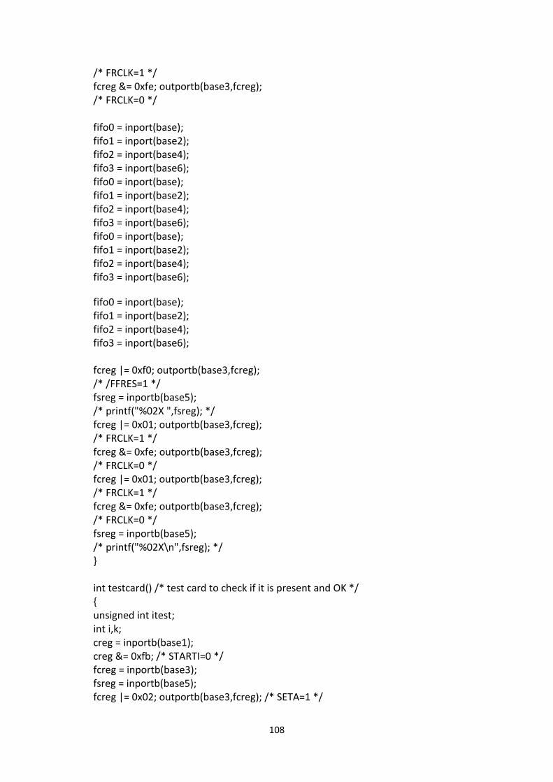
108
/* FRCLK=1 */ fcreg &= 0xfe; outportb(base3,fcreg); /* FRCLK=0 */ fifo0 = inport(base); fifo1 = inport(base2); fifo2 = inport(base4); fifo3 = inport(base6); fifo0 = inport(base); fifo1 = inport(base2); fifo2 = inport(base4); fifo3 = inport(base6); fifo0 = inport(base); fifo1 = inport(base2); fifo2 = inport(base4); fifo3 = inport(base6);
fifo0 = inport(base); fifo1 = inport(base2); fifo2 = inport(base4); fifo3 = inport(base6); fcreg |= 0xf0; outportb(base3,fcreg); /* /FFRES=1 */ fsreg = inportb(base5); /* printf("%02X ",fsreg); */ fcreg |= 0x01; outportb(base3,fcreg); /* FRCLK=1 */ fcreg &= 0xfe; outportb(base3,fcreg); /* FRCLK=0 */ fcreg |= 0x01; outportb(base3,fcreg); /* FRCLK=1 */ fcreg &= 0xfe; outportb(base3,fcreg); /* FRCLK=0 */ fsreg = inportb(base5); /* printf("%02X\n",fsreg); */ int testcard() /* test card to check if it is present and OK */ unsigned int itest; int i,k; creg = inportb(base1); creg &= 0xfb; /* STARTI=0 */ fcreg = inportb(base3); fsreg = inportb(base5); fcreg |= 0x02; outportb(base3,fcreg); /* SETA=1 */

109
outport(base8, 0xA5A8); outport(base10, 0xBBBB); /* P=BBBBA5A8 */ itest = inport(base8) & 0xFFF8; if(itest != 0xA5A8)return FALSE; fcreg |= 0x08; outportb(base3,fcreg); /* SEV=1 */ creg |= 0x08; outportb(base1,creg); /* ENA=1 */ creg |= 0x02; outportb(base1,creg); /* ENDR=1 */ creg |= 0x04; outportb(base1,creg); /* STARTI */ creg &= 0xfb; /* FS */ for (k=0; k<1024; k++) for (i=0; i<4; i++) fsreg = inportb(base5); if(fsreg & 0x40)break; fifo3 = inport(base10); if(fsreg & 0x40) fifo3 = inport(base6); fifo2 = inport(base4); fifo1 = inport(base2); fifo0 = inport(base); if (fifo3 != 0xBBBB) return FALSE; if (fifo2 != itest) /* may be new firmware version */ if (fifo2==0xA5A9 && itest==0xA5A8) itest++; else return FALSE; if (fifo1 != 0xAAAA) return FALSE; if (fifo0 != 0xAAAA) return FALSE; else return FALSE; /* printf("geht nicht! (OR == 0)\n"); */ itest++; return TRUE;
int lw7886_init(unsigned int newbase) base = newbase; base1 = base+1; base2 = base+2; base3 = base+3; base4 = base+4;

110
base5 = base+5; base6 = base+6; base8 = base+8; base10 = base+10; cardreset(); creg = inportb(base1); fcreg = inportb(base3); fsreg = inportb(base5); if (!(creg & 0x04)) return FALSE; /* OFF != 1 -> no 7886 found! */ creg = (creg & 0xfb); /* STARTI=0 */ fiforeset(); if (!testcard()) return FALSE; cardreset(); fiforeset(); return TRUE; int lw7886_acq(unsigned int *buffer, int range, in sweeps, double timeout) int hitim; unsigned int I; int amount; int range5; int counter=0; double starttime; unsigned int preset; creg = inportb(base1); creg = (creg & 0xfb); /* STARTI=0 */ fcreg = inportb(base3); fsreg = inportb(base5); starttime=Timer(); range &=0xffffff00; range5=range>>5; preset=(unsigned)-range5; fiforeset(); creg &= 0xfe; outportb(base1,creg); /* runs("mode=0"); */ creg &= 0xfd; outportb(base1,creg); /* runs("endr=0"); */ outpw (base8, (preset & 0x0000fff8)|0x3); outpw (base10, (preset & 0xffff0000)>>16); creg &= 0xf7; outportb(base1,creg); /* runs("ena=0"); */ creg |= 0x02; outportb(base1,creg); /* runs("endr=1"); */ creg |= 0x08; outportb(base1,creg); /* runs("ena=1"); */ for(;;) /*Dummy read until output ready*/

111
if(inpw(base8)& 0x02) while(inp(base5)&0x40) fifo3=inpw(base6); fifo2=inpw(base4); fifo1=inpw(base2); fifo0=inpw(base); hitim=(fifo0+fifo3*65536-preset)<<5; if (fifo0 & 0x01) ss[hitim]++; if (fifo0 & 0x02) ss[1+hitim]++; if (fifo0 & 0x04) ss[2+hitim]++; if (fifo0 & 0x08) ss[3+hitim]++; if (fifo0 & 0x10) ss[4+hitim]++; if (fifo0 & 0x20) ss[5+hitim]++; if (fifo0 & 0x40) ss[6+hitim]++; if (fifo0 & 0x80) ss[7+hitim]++; if (fifo0 & 0x0100) ss[8+hitim]++; if (fifo0 & 0x0200) ss[9+hitim]++; if (fifo0 & 0x0400) ss[10+hitim]++; if (fifo0 & 0x0800) ss[11+hitim]++; if (fifo0 & 0x1000) ss[12+hitim]++; if (fifo0 & 0x2000) ss[13+hitim]++; if (fifo0 & 0x4000) ss[14+hitim]++; if (fifo0 & 0x8000) ss[15+hitim]++; if (fifo1 & 0x01) ss[16+hitim]++; if (fifo1 & 0x02) ss[17+hitim]++; if (fifo1 & 0x04) ss[18+hitim]++; if (fifo1 & 0x08) ss[19+hitim]++; if (fifo1 & 0x10) ss[20+hitim]++; if (fifo1 & 0x20) ss[21+hitim]++; if (fifo1 & 0x40) ss[22+hitim]++; if (fifo1 & 0x80) ss[23+hitim]++; if (fifo1 & 0x0100) ss[24+hitim]++; if (fifo1 & 0x0200) ss[25+hitim]++; if (fifo1 & 0x0400) ss[26+hitim]++; if (fifo1 & 0x0800) ss[27+hitim]++; if (fifo1 & 0x1000) ss[28+hitim]++; if (fifo1 & 0x2000) ss[29+hitim]++; if (fifo1 & 0x4000) ss[30+hitim]++; if (fifo1 & 0x8000) ss[31+hitim]++; outpw(base8,inpw(base8)|0x02); counter++;

112
if (counter==sweeps) return counter; if(Timer()-starttimer>timeout) return counter;
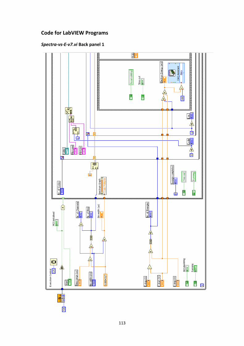
113
Code for LabVIEW Programs
Spectra-vs-E-v7.vi Back panel 1

114
Spectra-vs-E-v7.vi Back panel 2

115
Spectra-vs-E-v7.vi Back panel 3

116
multigauss test.vi Back panel 1

117
multigauss test.vi Back panel 2