STUDY OF DEEP EARTH STRUCTURE USING

CORE PHASES AND THEIR SCATTERED

ENERGY RECORDED AT

SEISMIC ARRAYS

Zuihong Zou, M.S.

An Abstract Presented to the Faculty of the Graduate

School of Saint Louis University in Partial

Fulfillment of the Requirements for the

Degree of Doctor of Philosophy

2008

Abstract

In the thesis, I endeavor to explore the structure of the Earth’s deep interior by an-

alyzing seismic core phases and their related scattered energy generated by small-scale

heterogeneities inside the Earth. By modeling the differential traveltimes and amplitude

ratios between PKP-DF and PKP-Cdiff measured from a large dataset recorded at seismic

arrays, I find that the optimum model by fitting the differential travel times has relatively

low velocity at the base of the outer core as in AK135, however, the optimum model found

by fitting the amplitude ratios does not exhibit this feature, and instead is closer to PREM.

The discrepancy may be explained by small-scale topography on the inner core boundary

(ICB) or a thin layer with relatively low Q at the base of the outer core. I also analyzed the

coda waves following PKP-Cdiff to locate the lateral heterogeneity and to attempt to un-

derstand its nature. By combined modeling of the travel times, slownesses, and envelopes

of the coda waves, I find a very strong heterogeneity in the lowermost mantle beneath

the Amazon River in South America. To examine the strength of small-scale random het-

erogeneities in the mantle, I assembled a large, geographically diverse data set of PKP

precursor envelopes from globally distributed international monitoring system seismic ar-

rays. I find that the amplitudes of the precursors change from region to region, and exhibit

significant variations within specific geographic regions. This may imply that the lower

mantle is not perfectly mixed by mantle convection, and that compositional heterogeneities

can survive in the mantle for billions of years. By modeling the globally averaged PKP

precursors using a seismic phonon method, my results show that a model with random het-

erogeneities at a scale-length of 8 km with 0.05% r.m.s. velocity perturbation uniformly

distributed throughout the lower mantle can provide a reasonable fit to the observations.

On the contrary, confining the heterogeneities near the core mantle boundary (CMB) or in

the D” does not yield the amplitude versus time pattern observed in our data. Furthermore,

extra scattering near the CMB or in the D” is not justified.

1

STUDY OF DEEP EARTH STRUCTURE USING

CORE PHASES AND THEIR SCATTERED

ENERGY RECORDED AT

SEISMIC ARRAYS

Zuihong Zou, M.S.

A Dissertation Presented to the Faculty of the Graduate

School of Saint Louis University in Partial

Fulfillment of the Requirements for the

Degree of Doctor of Philosophy

2008

c©Copyright by

Zuihong Zou

ALL RIGHTS RESERVED

2008

i

COMMITTEE IN CHARGE OF CANDIDACY:

Associate Professor Keith D. Koper,

Chairperson and Advisor

Professor Robert B. Herrmann

Associate Professor Lupei Zhu

ii

Acknowledgments

First of all, I owe the deepest gratitude to my parents and my siblings. It is your un-

conditional love and support that gave me beautiful dreams and made my dreams come

true.

I am deeply grateful to my advisor, Dr. Keith D. Koper, for his kindness, guidance,

advice, support, and stimulating discussions throughout my PhD study and research at

SLU. It was his suggestions and ideas that guided me through all the ups and downs of my

research to reach this point. I am so grateful for the four years’ great learning experiences,

which will be extremely beneficial to my future career.

I deeply thank Dr. Lupei Zhu and Dr. Robert B. Herrmann for their careful and detailed

reviews of the thesis and their persistent help and advice during my four years of graduate

study at SLU. I thank Dr. David J. Crossley, Dr. John Encarnacion, Dr. Timothy M. Kusky,

Dr. David Kirschner and Dr. Brian J. Mitchell. The knowledge and skills I’ve learned

from them will be a priceless fortune for the rest of my life. Thank you all so much for

your teaching, advice, sharing your experiences, kindness and friendship. And also, I must

acknowledge my master’s thesis advisor, Dr. Xiaofei Chen at Peking University, who had

a significant influence on my research interest and has been helping and encouraging me

persistently.

Each article in this thesis was made possible with the help of my advisor, collaborators

and colleagues. I wish to thank Dr. Vernon Cormier, Dr. Felipe Leyton, Dr. Peter Shearer

and Kevin Seats for their contributions. I thank Dr. Xiaodong Song, Dr. Satoru Tanaka, Dr.

Christine Thomas and several anonymous reviewers for their insightful and constructive

comments of the manuscripts. The financial support of the PhD research work came from

the graduate assistantship of Saint Louis University, NSF grants under contracts EAR-

0229103, EAR-0229586, EAR-050537438 and EAR-0296078.

I would also like to take this opportunity to extend my gratitude to all the geoscience

students. Thank you for your friendship and help to make my four years at SLU happy, en-

iii

joyable and memorable. Special thanks to my dear friends and colleagues: Hongyi, Felipe,

Ali, Michelle, Sabreen, Boston, Kevin, Oner, Hongfeng, Risheng, Young-Soo, Nathalie,

Sebastiano and Safat. The help and friendship from many friends at University of Illi-

nois were essential for me to get through the first year in the US, especially the help from

Zhaohui, Xinlei, Fang, Jingyun, Ellen, Mo, and Hsiang-Hsin.

I want to thank all the staff in the Earth and Atmosperic Sciences Department at SLU.

Bob Wurth and Eric Haug helped me to solve many computer-related issues. I thank them

for their support during my four years’ stay in the department. Those interesting and fun

chats with Melanie in Maclewane Hall made my life more enjoyable.

At last, I would like to express my deepest gratitude to my husband, Chuntao Liang,

for his love, caring, encouragement, support, and cheering me up ... I am deeply sorry for

your 50,000 miles driving on highways during the completion of this thesis. No words can

express how much I appreciate what you have done for me. Thank you, very much.

iv

Table of Contents

List of Tables vii

List of Figures viii

CHAPTER 1: Introduction 1

CHAPTER 2: The Structure of the Base of the Outer Core Inferred from Seis-

mic Waves Diffracted Around the Inner Core 6

2.1 Introduction . . . . . . . . . . . . . . . . . . . . . . . . . . 7

2.2 Assembly of PKPCdiff Waveform Database . . . . . . . . 10

2.3 Analysis of Differential Travel Times (PKPCdiff -PKPDF ) 13

2.3.1 Data Processing . . . . . . . . . . . . . . . . . . . 13

2.3.2 Data Modeling . . . . . . . . . . . . . . . . . . . . 16

2.4 Analysis of Amplitude Ratios (PKPCdiff /PKPDF ) . . . . 19

2.4.1 Data Processing . . . . . . . . . . . . . . . . . . . 19

2.4.2 Data Modeling . . . . . . . . . . . . . . . . . . . . 21

2.5 Discussion . . . . . . . . . . . . . . . . . . . . . . . . . . . 25

2.5.1 Hypothesis #1: A Rough ICB . . . . . . . . . . . . 26

2.5.2 Hypothesis #2: A Slurry Zone at the Base of the

Outer Core . . . . . . . . . . . . . . . . . . . . . . 27

2.6 Conclusions . . . . . . . . . . . . . . . . . . . . . . . . . . 29

CHAPTER 3: Partial Melt in the Lowermost Mantle Near the Base of a Plume 32

3.1 Introduction . . . . . . . . . . . . . . . . . . . . . . . . . . 33

3.2 Data . . . . . . . . . . . . . . . . . . . . . . . . . . . . . . 35

3.3 Ray Parameter of PKPCdiff Coda . . . . . . . . . . . . . . 35

v

3.4 The Origin of the PKPCdiff Coda . . . . . . . . . . . . . . 41

3.5 Conclusions and Discussion . . . . . . . . . . . . . . . . . 48

CHAPTER 4: Using PKP Precursors Recorded at IMS Arrays to Determine

the Small-scale Heterogeneity in the Mantle 50

4.1 Introduction . . . . . . . . . . . . . . . . . . . . . . . . . . 51

4.2 Data Processing . . . . . . . . . . . . . . . . . . . . . . . . 55

4.3 Modeling Global Average PKP Precursor Envelopes . . . . 60

4.4 Regional Variations of PKP Precursor Amplitude . . . . . 70

4.5 Conclusions and Discussion . . . . . . . . . . . . . . . . . 73

APPENDIX: Copyright Permission 75

References 77

Vita Auctoris 90

vi

List of Tables

Table 2.1: Events and seismic arrays used in this study . . . . . . . . . . . . . . 13

Table 4.1: IMS seismic arrays used and the number of events selected . . . . . . 56

vii

List of Figures

Figure 2.1: P-wave velocity structure near the ICB . . . . . . . . . . . . . . . . 8

Figure 2.2: Ray path for PKP waves . . . . . . . . . . . . . . . . . . . . . . . 9

Figure 2.3: An example of a vertical seismic record section . . . . . . . . . . . 11

Figure 2.4: The great circle paths from earthquakes to arrays . . . . . . . . . . . 12

Figure 2.5: Observed PKPCdiff − PKPDF differential times . . . . . . . . . . 17

Figure 2.6: Synthetic tests for factors affecting travel times . . . . . . . . . . . 18

Figure 2.7: The best fitting model from the differential times . . . . . . . . . . . 20

Figure 2.8: Observed amplitude ratios . . . . . . . . . . . . . . . . . . . . . . . 22

Figure 2.9: Synthetic tests for amplitude ratios . . . . . . . . . . . . . . . . . . 24

Figure 3.1: Source-receiver geometry for the seismic data . . . . . . . . . . . . 36

Figure 3.2: Vertical component record section . . . . . . . . . . . . . . . . . . 37

Figure 3.3: Event 990302 . . . . . . . . . . . . . . . . . . . . . . . . . . . . . 38

Figure 3.4: Event 990305 . . . . . . . . . . . . . . . . . . . . . . . . . . . . . 39

Figure 3.5: Comparison of waveforms of the empirical source . . . . . . . . . . 41

Figure 3.6: Comparison between synthetic seismograms and data . . . . . . . . 42

Figure 3.7: Properties of the geometrical scattered waves . . . . . . . . . . . . 45

Figure 3.8: Trade-off between scattering volume . . . . . . . . . . . . . . . . . 47

Figure 4.1: Ray paths and travel time curves for the core phases and precursors . 53

Figure 4.2: Geometry of IMS seismic arrays . . . . . . . . . . . . . . . . . . . 57

Figure 4.3: Vertical record section of an example event and its sliding window

slowness analysis . . . . . . . . . . . . . . . . . . . . . . . . . . . . . . . 58

Figure 4.4: Average precursor amplitudes as a function of time and distance . . 61

Figure 4.5: Comparison of observed precursor and predicted precursor . . . . . 63

Figure 4.6: Comparison of observed precursor and predicted precursor . . . . . 65

viii

Figure 4.7: Comparison of observed precursor and predicted precursor . . . . . 66

Figure 4.8: Comparison of observed precursor and predicted precursor . . . . . 67

Figure 4.9: Comparison of observed precursor and predicted precursor . . . . . 68

Figure 4.10: Comparison of observed precursor and predicted precursor . . . . . 69

Figure 4.11: The standard deviations of the globally averaged precursors’ ampli-

tudes . . . . . . . . . . . . . . . . . . . . . . . . . . . . . . . . . . . . . . 71

Figure 4.12: The geographical distribution of precursors . . . . . . . . . . . . . . 72

ix

Chapter 1

Introduction

The Earth is a complex and quasi-spherical body with a radius of ∼ 6371 km. Seismo-

logical studies during the last 100 years have revealed in great detail the 1-D radial Earth

structure. The seismogram is the primary resource that scientists rely on to explore the

structure of the Earth’s deep interior. Although the basic theory needed to interpret the

observations was well developed in the early 1800s, the development of seismic instru-

mentation was behind the theory, which prevented scientists from achieving breakthroughs

in discovering the Earth’s interior structure until 1900s. In 1900, Richard Oldham identi-

fied P , S, and surface waves from seismograms and discovered the Earth’s liquid core a

few years later based on the P -wave shadow zone (Oldham, 1906). Following Oldham’s

notice of the P -wave shadow zone, Gutenberg estimated the depth of the boundary be-

tween the mantle and the liquid core to be about 2900 km for the first time (Gutenberg,

1913), which is very close to the value of 2891 km, obtained from modern seismic data

in the Preliminary Reference Earth Model (PREM) (Dziewonski and Anderson, 1981). In

1909, Andrija Mohorovicic unveiled the discontinuity between the lower density crust and

the higher density mantle through his meticulous analyses of two sets of waves from one

earthquake. In 1936, Inge Lehmann discovered a weak P wave in the shadow zone and

hypothesized the existence of a solid inner core within the liquid core (Lehmann, 1936),

which was confirmed by other scientists later (Birch, 1940; Dziewonski and Gilbert, 1971).

By the 1940s, the concept that the travel times of seismic arrivals can be used to infer

the velocity structure of the Earth was well established and scientists agreed on the 1-D

layered Earth structure (from the surface to the center are the crust, the mantle, the outer

core and the inner core). The JB tables which contain the arrival times of seismic phases

were published by Jeffreys and Bullen in 1940 and are still good reference today. Since

then, the availability of more and more modern seismic data has led to rapid progress in

1

unveiling increasingly detailed structure of Earth’s interior. In the 1960s, there was enough

evidence to support the existence of seismic velocity discontinuities at depths of about

410 km and 660 km (e.g. Niazi and Anderson, 1965; Johnson, 1967; Anderson, 1967). The

thickness and topography of the transition zone (the layer between the two discontinuities)

are still under scrutiny (see Shearer 2000 for a review). Now all modern 1-D reference

Earth models, such as PREM, AK135 (Kennett et al., 1995), and IASP91 (Kennett and

Engdahl, 1991), include those seismic discontinuities at only slightly different depths. In

the mean time, more sophisticated imaging techniques have led to many interesting break-

throughs about the large-scale lateral heterogeneity inside the Earth. For instance, global

tomography revealed the fate of subducted slabs and the origin of upwelling plumes (e.g.

Grand et al., 1997; van der Hilst et al., 1997; Montelli et al., 2004; Lei and Zhao, 2006).

Most of the findings about the 1-D Earth structure so far have been achieved by analyz-

ing the travel times and waveforms of the main seismic phases. The large-scale non-radial

structures are mostly revealed by seismic tomography (both the traditional ray-theory to-

mography and the new finite-frequency tomography). The travel times and waveforms of

main phases predicted by 1-D Earth models are still the most important tools to image

the large-scale structure of the Earth. However, resolving the small-scale structure (with

a scale of 5-10 km) is beyond the resolution of seismic tomography because of the spatial

aliasing and contamination of waves scattered by the strong heterogeneites inside the Earth.

High-frequency coda waves following P or S waves are direct evidence for small-scale ran-

dom heterogeneity in the lithosphere. Aki (1969) first showed that the scattered coda waves,

which used to be treated as noise, can be used to estimate the strength of the random hetero-

geneity. Observations of PKP precursors concluded that small-scale heterogeneity must

also exist in the deep mantle (Doornbos and Husebye, 1972; Cleary and Haddon, 1972).

More recently, small-scale heterogeneity inside the inner core has also been discovered by

many different authors (e.g. Vidale and Earle, 2000; Cormier and Li, 2002; Koper et al.,

2004; Leyton and Koper, 2007). In order to obtain a high-resolution image of the Earth’s

interior to better understand the nature of the small-scale heterogeneities and the dynamics

of the whole Earth, we must put a great effort to the analysis of high-frequency scattered

energy.

2

In this dissertation, I attempted to explore the interior structure of the Earth by analyzing

the seismic core phases and their related scattered energy generated by small-scale hetero-

geneities inside the Earth, which may arrive before or after the main phases (coda waves or

precursors). Guided by this intention, the dissertation is composed of four chapters. This

chapter (Chapter 1) is an overview of the whole dissertation, which introduces previous

related work and the motivations of my work. Each one of the following three chapters

(Chapter 2 - Chapter 4) consists of an independent paper addressing different issues, thus

having the complete structure of a standard journal paper. At the time of publication of the

thesis, Chapter 3 has been published in Geophysical Journal International (see Zou et al.,

2007) with the corresponding copyright permission shown in the Appendix; Chapter 2 has

been accepted for publication in Journal of Geophysical Research; while Chapter 4 is in

preparation for submission to Journal of Geophysical Research.

The velocity structure of the inner core boundary (ICB) plays an important role for us

to understand the chemical composition and dynamics of the core. The velocity gradient

can be linked to the density gradient. The widely used reference Earth model PREM has a

uniform composition throughout the outer core. However, some more recent models such

as AK135 and PREM2 (Song and Helmberger, 1995) have a reduced velocity gradient at

the base of the outer core, which implies some sort of chemical heterogeneity there. In

Chapter 2, I followed the traditional seismological methods to examine the travel time and

amplitude of PKPCdiff , which is the wave that diffracts around the inner core boundary

(ICB), to infer the velocity structure at the base of the outer core. In the past, systematic

study of PKPCdiff at distances greater than 154◦ was not conducted because this phase

is only observable over a very limited range of source-receiver distances, has relatively

small amplitude, and thus is difficult to observe. The proliferation of regional broadband

arrays over the last decade has made the observations of PKPCdiff waves less difficult

because closely-spaced seismic arrays allow small coherent phases to be identified and

isolated, and slowness estimates can be made to verify the identity of prospective phases.

By assembling a large, high-quality set of PKPCdiff waveforms from seismic arrays, I

was able to constrain the velocity structure at the base of the outer core and then to learn

about the chemistry and dynamics of the core.

3

As I examined PKPCdiff waves, I noticed strong coda waves following PKPCdiff for

one of the events recorded at INDEPTH-III (International Deep Profiling of Tibet and the

Himalayas Phase III) array. However, two other nearby events do not show these prominent

coda waves. The scattered coda waves recorded at arrays are very useful to locate the

scatterer in the deep Earth if we can carefully model their travel times, slownesses, and

amplitudes. The PKPCdiff coda waves have been reported and investigated by several

authors. For example, Tanaka (2005) presented characteristics of PKPCdiff coda waves

from the small-aperture array short-period stations of the International Monitoring System.

He observed a wide range of slownesses for the PKPCdiff coda waves, and interpreted the

coda waves with slowness larger than 2 s/deg as scattering from the core-mantle boundary

under the source side and receiver side, although an ICB origin could not be ruled out. In

Chapter 3, I presented an analysis of a high-quality PKPCdiff record section recorded by

a temporary array of broadband seismometers in Tibet from the INDEPTH-III experiment.

I was able to model the differential travel times and slownesses relative to PKPDF , and

envelopes of the coda using single-scattering theory to locate the anomalous region and

obtain its velocity perturbation.

The scattered energy generally arrives after the main phase as coda, however, the spe-

cial velocity structure at the CMB can cause the scattered energy from the heterogeneities

in the mantle to arrive before the main phase PKIKP as precursors. This type of scattered

energy preceding PKP was first observed in 1934 (Gutenberg and Richter, 1934). Previ-

ous studies of the PKP precursors had controversy about their origin, including refraction

in the inner core (Gutenberg, 1957), refraction or reflection in a transition layer between

the outer and inner cores (Bolt, 1962; Sacks and Saa, 1969), and diffraction from the CMB

(Bullen and Burke-Gaffney, 1958). It is now widely accepted that PKP precursors are

generated by the scattering from volumetric inhomogeneities near the CMB or within the

lower mantle, or from CMB topography (Doornbos and Husebye, 1972; Cleary and Had-

don, 1972; Bataille et al., 1990). However, the radial and lateral distributions, as well as

the magnitude of the small-scale mantle heterogeneity are still not well resolved. Modeling

of global average precursors tends to favor a whole mantle scattering model instead of con-

fining the heterogeneity near the CMB. However, the magnitude of P -wave velocity per-

4

turbation among different studies varies by a factor of ten. The discrepancy come from two

possible causes. One is related to the data used in different studies. Due to uneven data sam-

pling and different data processing schemes, different authors may obtain different global

average PKP precursor envelopes. The other possible reason may be related to differences

in forward modeling methods. For the same precursors, the single-scattering theory may

yield different magnitudes of heterogeneity from a multiple-scattering or diffusion-based

theory. In Chapter 4, I assembled a large, geographically diverse dataset of PKP pre-

cursor envelopes by using the globally distributed International Monitoring System (IMS)

seismic arrays. An advantage of using arrays over single stations is that the recordings of

all elements at one array can be coherently stacked to suppress noise, and thus obtain high

signal-to-noise (SNR) ratio PKP precursors, even for relatively small earthquakes. I then

used a type of Monte-Carlo seismic phonon method to model the globally averaged PKP

precursor envelopes to learn about the small-scale heterogeneities in the mantle, which may

provide some insights about mantle dynamics.

5

Chapter 2

The Structure of the Base of the Outer Core

Inferred from Seismic Waves Diffracted Around

the Inner Core

We systematically searched for seismograms of waves diffracted around the inner core

(PKPCdiff ) from all the temporary seismic arrays with data currently available at the IRIS

DMC, as well as some permanent regional seismic arrays including F-NET in Japan and

GRF in Germany, to assemble the largest high-quality PKPCdiff database ever created.

PKPCdiff waves preferentially sample the base of the outer core and so contain important

clues about Earth structure in this region. We measured PKPDF − PKPCdiff differential

travel times and PKPCdiff/PKPDF amplitude ratios in the distance range of 154◦− 160◦

and modeled the observations using grid searches and full wave theory synthetic seismo-

grams. The optimum model found by fitting the differential travel times has relatively low

velocity at the base of the outer core as in AK135, which is consistent with many previ-

ous travel time studies. However, the optimum model found by fitting the amplitude ratios

(PKPCdiff/PKPDF ) does not exhibit this feature, and instead is closer to PREM. The

discrepancy may be explained by two likely causes. One is that small-scale topography or

roughness on the ICB tends to scatter energy away from PKPCdiff waves by generating

trailing coda waves. The other is that there exists a thin layer with relatively low Q at the

base of the outer core. This might be expected if there are suspended solid particles at the

base of the outer core, as proposed decades ago. Both mechanisms could generate smaller

PKPCdiff amplitudes without significantly affecting PKPCdiff travel times.

6

2.1 Introduction

A large number of seismological studies have suggested that the region just above the

inner core boundary (ICB) is distinct from the rest of the outer core. The layer about 400 km

above the ICB was originally termed the F-layer and was characterized by a strong low

velocity zone (Jeffreys, 1939). Later Earth models, constructed with more accurate travel

time data, instead defined this as a region of increased velocity, and often included one

or more first order discontinuities above the ICB (Bolt, 1962, 1964; Adams and Randall,

1964; Sacks and Saa, 1969). Ultimately though, these model types were also discarded,

as PKP precursors were reinterpreted as energy scattered from mantle heterogeneities near

the core mantle boundary (CMB) (Doornbos and Husebye, 1972; Cleary and Haddon,

1972; Haddon and Cleary, 1974). Hence, modern reference Earth models universally have

smoothly increasing velocities at the base of the outer core.

There is still some uncertainty, however, about the steepness of the velocity gradient at

the base of the outer core. This is important because the velocity gradient strongly con-

strains the density gradient in the Earth’s core. If we assume the pressure derivative of the

bulk modulus is constant (∼3.5) in the outer core (Anderson and Ahrens, 1994), then the

Bullen parameter η (Bullen, 1963), which is the ratio between the actual density gradient

and the gradient corresponding to uniform composition, only depends on the velocity gra-

dient. The widely used reference Earth model PREM (Dziewonski and Anderson, 1981)

has the Bullen parameter η ∼ 1 through the outer core, which implies a homogeneous,

adiabatic medium.

More recent reference Earth models, such as PREM2 (Song and Helmberger, 1995)

and AK135 (Kennett et al., 1995), have significantly lower velocity gradients at the base of

the outer core, corresponding to Bullen parameters significantly higher than 1 (Figure 2.1).

In other words, these models imply that near the base of the outer core density increases

too quickly to be explained solely by compression, and some sort of change in chemistry

or phase must occur. Interestingly, core dynamical studies suggested a slurry layer occu-

pied by free-floating broken dendrites just above the ICB several decades ago (Loper and

Roberts, 1978; Loper, 1978; Loper and Roberts, 1981). However, more recent studies con-

7

10.0

10.2

10.4

10.6

10.8

11.0

11.2

Vel

ocity

(km

/s)

800 900 1000 1100 1200 1300 1400 1500 1600Radius(km)

PREM2AK135PREM

Figure 2.1: P-wave velocity structure near the ICB. The radius of ICB in AK135 is shiftedto be the same as PREM and PREM2. Dashed curve is for PREM, solid one is for PREM2and dotted curve is for AK135. AK135 is nearly identical to PREM2 at the base of theouter core.

sider a slurry of suspended particles unlikely to exist in the Earth and instead suggest that

a thin mushy zone is more probable (Bergman, 2003; Shimizu et al., 2005).

But not all seismic studies support a relatively low velocity gradient at the base of

the outer core. Choy and Cormier (1983) found that KOR5 predicts too large PKPCdiff

amplitudes compared to the observations and ruled out the low velocity gradient zone above

the ICB, which is consistent with their previous results (Rial and Cormier, 1980; Cormier,

1981). Both Huang (1996) and Kaneshima et al. (1994) investigated the ICB velocity

structure beneath North America’s Pacific seashore and they obtained a slightly smaller P-

wave velocity than that in PREM, but significantly larger than that in AK135 at the base of

the outer core. Most recently Yu et al. (2005) re-examined the outer core velocity structure

by analyzing differential travel times, amplitude ratios and waveforms of various PKP

waves recorded at Global Seismograph Network (GSN) and several regional networks and

they found out that the velocity structure at the base of the outer core exhibited a strong

hemispherical difference. The data sampling the quasi-eastern hemisphere (40◦W-180◦E)

can be explained by a PREM-type outer core velocity structure, while those sampling the

8

1050

1100

1150

1200

1250

1300

Tra

vel t

ime

(s)

120 130 140 150 160 170 180Distance (deg)

Cdiff

innercore

outer core

mantle

B

C

A

D

FDF 0˚

30˚

60˚

90˚

120˚

150˚

180˚210˚

240˚270˚

300˚

330˚

AB

Figure 2.2: (Left) Ray path for PKP waves at the C-cusp for an event at 400 km depth.Black curve represents the ray path of PKPDF at a distance of 156◦. Gray curves indicatetheray paths of PKP waves diffracted along the ICB. (Right) Standard travel time curveforPKP waves in PREM. The dashed line indicates propagation of PKPCdiff .

quasi-western hemisphere (180◦W-40◦E) can be best explained by their preferred model

OW, which has velocity closer to PREM2 than PREM at the base of the outer core.

In this study, we focus on studying the structure of the base of the outer core by an-

alyzing PKPCdiff waves, which are waves diffracted around the ICB and are more sen-

sitive to the base of the outer core than any other phase. Although ray theory predicts

zero amplitude after the C-cusp (Figure 2.2), which occurs at a distance of ∼ 152.5◦ in

PREM or ∼ 155.5◦ in AK135 for a source at 100 km depth, both theoretical calculations

(Cormier and Richards, 1977; Cormier, 1981) and observations (Huang, 1996) indicate

that PKPCdiff has significant energy for several degrees into the inner core shadow zone.

At these distances the amplitude decay of PKPCdiff is mainly controlled by diffraction

and is extremely sensitive to the velocity gradient just above the ICB and the period of

PKPCdiff .

Systematic study of PKPCdiff at distances greater than 154◦ has been somewhat ne-

glected because it is difficult to observe. Small earthquakes do not generate PKPCdiff

waves large enough to be observed above the background noise, and large earthquakes

usually have long source durations, which makes PKPDF interfere with PKPCdiff (the

time separation between them is less than 10 s). Similarly, shallow earthquakes sometimes

9

generate PKPDF depth phases that interfere with PKPCdiff , though with careful model-

ing of the source time functions this problem can often be overcome.

The proliferation of regional broadband arrays over the last decade has made the ob-

servations of PKPCdiff waves less difficult, and has enabled us to assemble a large, high-

quality set of PKPCdiff waveforms. In order to reduce shallow structure effects, we use

PKPDF as a reference phase since it has a ray path very similar to PKPCdiff in the crust

and mantle. Although the top of the inner core always has an effect on the travel time and

amplitude of PKPDF , our synthetic tests show that this effect is small compared with the

effect of the base of the outer core on PKPCdiff . Therefore, the differential travel times

and amplitude ratios between PKPDF and PKPCdiff measured from the high-quality

record sections provide an excellent opportunity to explore the structure at the base of the

outer core.

2.2 Assembly of PKPCdiff Waveform Database

Because PKPCdiff is only observable over a very limited range of source-receiver

distances and has relatively small amplitude, a closely-spaced seismic array is important to

identify the phase and to generate a high-quality PKPCdiff data set. An array allows small

coherent phases to be identified and isolated, and slowness estimates can be made to verify

the identity of prospective phases. Another advantage is that the differential travel times

(PKPCdiff − PKPDF ) can be measured more accurately by cross-correlating waveforms

in the PKPCdiff time window and the PKPDF time window respectively, instead of cross-

correlating the PKPCdiff window with the PKPDF window for a single station. This is

especially important because diffracted waves undergo some shape change as they arrive at

larger distances, and so they have shapes dissimilar with PKPDF .

We systematically examined the waveforms of earthquakes with depth greater than

60 km and magnitude greater than 5.5 Mw from all the temporary PASSCAL networks

with data open to public researchers at the IRIS DMC, as well as some permanent re-

gional seismic arrays such as F-NET (Full Range Seismograph Network of Japan) and GRF

(Grafenberg) array in Germany. Deep earthquakes have relatively short source durations,

10

153

154

155

156

157

158

159

160

161

Dis

tanc

e(de

g)

1150 1160 1170 1180 1190 1200 1210 1220 1230 Time (s)

PKPDF

PKPCdiff

PKPDF

PKPCdiff

PKPABPKPAB

(b)(a)

Dis

tanc

e(de

g)

153

154

155

156

157

158

159

160

161

1150 1160 1170 1180 1190 1200 1210 1220 1230 Time (s)

(b)

Figure 2.3: (a) An example of a vertical-component seismic record section which showsgood PKPDF and PKPCdiff waveforms from an event recorded at the F-net array with amagnitude of 6.1 Mw and a depth of 274 km (Event No. 4 in Table 2.1). Seismograms arefiltered around 3 s using band-pass filtering. (b) The corresponding synthetic seismogramscomputed from full-wave theory method for an explosivesource at a depth of 274 km basedon the PREM model.

which enables us to separate PKPDF and PKPCdiff more easily since the differential time

between these two phases is about 10 s. And deep sources avoid the potential interference

of the depth phase pPKPDF with PKPCdiff .

All the record sections in the distance range 154◦ − 160◦ were checked visually for

quality. We picked those events that have high signal-to-noise ratios (SNRs) records and

show clear PKPDF and PKPCdiff phases (Figure 2.3). The amplitudes of PKPCdiff

waves decay with distance and are almost at the noise level after a few degrees. In our

data selection criteria, we choose all the traces with high SNRs after 154◦ until the one at

which the PKPCdiff phase is no longer identifiable. We discuss the possible bias caused

by choosing only the “best” data in a later section of this manuscript.

As expected, the PKPCdiff waves are very difficult to observe. We examined 111

record sections from F-net, 110 record sections from GRF, and more than 300 record sec-

tions from the temporary networks at IRIS DMC in the distance range 154◦ − 160◦. The

11

0˚ 40˚ 80˚ 120˚ 160˚ 200˚ 240˚ 280˚ 320˚-90˚

-60˚

-30˚

0˚

30˚

60˚

90˚

Figure 2.4: The great circle paths from earthquakes to corresponding seismic arrays forhigh-quality PKPDF and PKPCdiff waveforms. The triangles are seismic arrays, the starsare earthquake locations,and the black circles indicate the turning point of PKPDF in theinner core.

total number of seismograms inspected was about 11,000. We obtained only 21 record sec-

tions, corresponding to 370 individual seismograms, which show high-quality PKPCdiff

waves. Table 2.1 lists all the events and the corresponding seismic arrays used in this

study. Among the 21 events in Table 1, 10 events were recorded at F-NET, 3 events were

recorded at GRF, 2 events were recorded by the BANJO/SEDA (Broadband Andean Joint

and Seismic Exploration of the Deep Altiplano) experiment, 2 events were recorded from

INDEPTH-II (International Deep Profiling of Tibet and Himalayas, Phase II) experiment

and 4 events were recorded by the INDEPTH-III experiment. Due to the small number of

high quality seismograms, the geographical sampling of the core by the PKPCdiff data

set is limited (Figure 2.4). Most of our data sample the quasi-western hemisphere (180◦W-

40◦E) with limited sampling points in the quasi-eastern hemisphere (40◦E-180◦E).

12

Table 2.1: Events and seismic arrays used in this study

Event EventTime Lat Lon Depth Mag Arraya #b φc

ID (yr/mon/day/hr:min) (◦N) (◦E) (km) (Mw) Code (◦)1 1997/07/20/10:14 -22.98 -66.30 256 6.1 FN 12 602 1999/11/21/03:51 -21.75 -68.78 101 5.8 FN 8 623 2000/06/16/07:55 -33.88 -70.09 120 6.4 FN 22 544 2001/06/29/18:35 -19.52 -66.25 274 6.1 FN 23 625 2002/09/24/03:57 -31.52 -69.20 119 6.2 FN 32 556 2003/09/17/21:34 -21.47 -68.32 127 5.7 FN 14 627 2004/09/11/21:52 -57.98 -25.34 64 6.1 FN 24 438 2005/06/12/19:26 -56.28 -26.98 95 6.0 FN 26 449 2005/06/13/22:44 -19.90 -69.13 111 7.7 FN 26 6310 2005/08/14/02:39 -19.74 -69.02 83 5.8 FN 12 6311 1994/06/16/18:41 -15.18 -70.34 225 5.9 DII 9 6712 1994/08/19/10:02 -26.65 -63.38 565 6.4 DII 8 6113 1994/09/28/17:33 -5.72 110.38 634 6.0 BS 18 8314 1994/11/15/20:18 -5.61 110.20 559 6.5 BS 14 8315 1998/10/08/04:51 -16.12 -71.40 136 6.1 DIII 27 6616 1999/03/02/17:45 -22.72 -68.50 110 5.9 DIII 27 6217 1999/03/05/00:33 -20.42 -68.90 110 5.8 DIII 27 6318 1999/04/03/06:17 -16.66 -72.66 87 6.8 DIII 30 6419 1995/10/14/08:00 -25.57 -177.51 70 6.2 GRF 13 5220 1997/04/12/09:21 -28.17 -178.37 184 5.9 GRF 13 5121 2001/03/11/00:50 -25.37 -177.97 231 5.8 GRF 13 53

a For the array code, FN stands for F-net, DII stands for INDEPTH-II, DIII stands forINDEPTH-III, BS stands for BANJO/SEDA, and GRF stands for Grafenberg.b # is the number of seismograms used in the record section.c φ is the angle of the turning direction of PKPDF in the inner core with respect to theEarth’s rotation axis.

2.3 Analysis of Differential Travel Times (PKPCdiff -PKPDF )

2.3.1 Data Processing

Differential PKPCdiff − PKPDF travel times from our data set are measured as fol-

lows. First for each record section, we filter velocity seismograms with a 3-pole Butter-

worth bandpass filter around 3 s with a one octave band. Although in theory filtering the

seismograms at different frequency bands can provide us a separate constraint about the

13

velocity structure at the base of the outer core, unfortunately, we found that it is difficult

to get accurate measurements of PKPCdiff − PKPDF travel times at higher or lower

frequencies. At longer periods, the short time interval between PKPDF and PKPCdiff

makes them interfere with each other (Souriau and Roudil, 1995). At higher frequencies,

noise and complicated waveforms prohibit cross-correlation from working properly to get

accurate travel time estimates. Around 3 s, PKPCdiff and PKPDF are well separated, and

we can obtain the most accurate measurements for the differential times and the amplitude

ratios.

After filtering, we use the multichannel cross-correlation method (mccc) (van Decar

and Crosson, 1990) to align the record section within the PKPDF time window to get

relative time shifts. Then we stack the aligned record section to get the time of the peak

amplitude. By using those relative time shifts and the time of the peak amplitude, we can

get the arrival times of PKPDF as described in van Decar and Crosson (1990). Repeating

the same procedure for PKPCdiff , we get the travel time of PKPCdiff and then the differ-

ential times PKPCdiff − PKPDF . The differential times measured by the mccc method

were compared with those obtained with the adaptive stacking technique (Rawlinson and

Kennett, 2004), which was proposed specifically for aligning waveforms with somewhat

dissimilar shapes. The methods give almost identical results for the PKPCdiff -PKPDF

differential times. For each record section, we also invert the arrival times yielded by mccc

for the slowness and back azimuth of PKPDF and PKPCdiff phases. We find that they

are generally very close to the predicted values in AK135 for most of the events, which

ensures that we are indeed analysing the proper phases. For a few events the deviations are

somewhat big, but in these cases the standard errors are also large because of poor source-

receiver geometry. As an example, we have poor backazimuth resolution for some events

recorded at INDEPTH-III because the strike of the array matches the expected backazimuth

(see Figure 1 of Zou et al. (2007)).

We apply this same method to predict PKPCdiff − PKPDF differential times for ar-

bitrary velocity models using synthetic seismograms calculated with the full-wave theory

technique (Cormier and Richards, 1977). This method works with spherically symmetric,

anelastic Earth models parametrized as polynomial functions of normalized radius. Full-

14

wave theory correctly accounts for the diffraction and tunnelling of body waves at and near

the grazing incidence to a boundary by incorporating the Langer approximation (Cormier

and Richards, 1988). This technique is computationally fast and because it operates in

spherical geometry it avoids the earth-flattening approximation. It has shown good agree-

ment with the reflectivity method (Choy et al., 1980) and the generalized ray method (Song

and Helmberger, 1992) for generating synthetic core phases. An example record section

is shown in Figure 2.3. We compared full wave theory synthetics to those calculated using

a frequency-wavenumber (fk) integration method (Zhu and Rivera, 2002; Herrmann and

Mandal, 1986) and found slightly different results; however, the fk synthetics contained

some artifacts that were presumably related to layering in a flattened Earth model.

Our observed PKPCdiff − PKPDF differential travel times are plotted relative to

PREM in Figure 2.5. The effect of different source depth is accounted for as follows. For

each event’s depth and distance, we find the PKPDF ray parameter predicted by PREM.

For that ray parameter, we find the corresponding distance for an event at 100 km depth,

which is the distance plotted in Figure 2.5. All the synthetics are computed with a source

depth at 100 km. Although the data are somewhat scattered, it appears that AK135 fits

the data better than PREM. We use a statistical method called an F -test (Menke, 1989) to

verify this quantitatively. First, we calculate the variances of the misfits between the data

and the predicted values from the two models, which are 0.1524 for AK135 and 0.2117

for PREM, respectively. The F value is then formed from the ratio of the two variances,

which is 1.3891. Using an F -calculater (http://faculty.vassar.edu/lowry/tabs.html), we find

that there is only a 0.16% probability that the two models are equal, which implies that

AK135 is better than PREM at a 99.8% probability in terms of fitting the data. However,

we do not observe obvious quasi-hemispherical differences in the data as seen for instance

by Yu and Wen (2006). Although the average differential travel time residual for the eastern

hemisphere (crosses in Figure 2.5) is a little bigger than for the western hemisphere (gray

dots in Figure 2.5), the scattering ranges of the data overlap. The reason for the lack of

a clear hemispherical signal may be that our data set is limited in the eastern hemisphere,

or because the hemispherical pattern of the inner core velocity observed by some studies

(Niu and Wen, 2001a; Wen and Niu, 2002; Garcia, 2002; Stroujkova and Cormier, 2004; Yu

15

et al., 2005; Yu and Wen, 2006) disappears at larger distances (such as the range considered

here) as reported by other authors (Garcia et al., 2006; Garcia, 2002; Cao and Romanow-

icz, 2004). This would be expected if the quasi-hemispherical pattern in the inner core

exists only to relatively shallow depths beneath the ICB.

2.3.2 Data Modeling

In modeling the travel time data we only vary the velocity structure at the base of the

outer core and fix the velocity in the remainder of the Earth according to PREM. There

are several reasons why this type of limited parametrization is justified. First, because the

ray paths of PKPDF and PKPCdiff are very close in the crust and most of the mantle,

the differential times can be attributed mainly to the velocity structure in the lower outer

core and at most the upper 500 km of the inner core. For our distance range of 154◦ −

160◦ the reference phase PKPDF turns at 300-500 km below the ICB, while PKPCdiff

has maximum sensitivity just above the ICB. Second, the difference in inner core and the

lowermost mantle velocity structure between standard reference models has very small

effects on PKPCdiff -PKPDF differential times, while the difference in the velocity at the

base of outer core between standard reference models has a large effect (Figure 2.6). Third,

we note that the angle of PKPDF with respect to Earth’s rotation axis for all our data

is greater than 45◦ (Table 2.1). Based on the reported inner core anisotropy models (e.g.

Creager, 1992; Shearer, 1994; Vinnik et al., 1994; Song and Richards, 1996), the travel

time difference of PKPDF caused by anisotropy is very small (less than 0.2 s). So the

observed differential times PKPCdiff − PKPDF would not be affected significantly by

inner core anisotropy. Fourth, we do not observe a strong quasi-hemispherical signal in the

data, and so separate modeling for each hemisphere is not warranted.

Among velocity models at the base of the outer core reported by different studies (e.g.

Qamar, 1973; Dziewonski and Anderson, 1981; Choy and Cormier, 1983; Souriau and

Poupinet, 1991; Song and Helmberger, 1995; Kennett et al., 1995; Yu et al., 2005), the main

difference is the structure of the velocity and its gradient at the bottom 400 km (or less) of

the outer core. In PREM (Dziewonski and Anderson, 1981), the velocity increases with a

16

-2.0

-1.5

-1.0

-0.5

0.0

0.5

1.0

1.5

2.0

Cdi

ff-D

F di

ffere

ntia

l tim

e

154 155 156 157 158 159 160 161Distance(deg)

PREM

AK135western hemisphere

eastern hemisphere

Figure 2.5: Observed PKPCdiff − PKPDF differential travel times relative to PREM.The solid line is for PREM, which is zero since it is used as a reference. The dashed linerepresents predicted differential times of AK135 relative PREM. The pluses are for the datasampling the eastern hemisphere, and the gray circles are for the data sampling the westernhemisphere.

17

(a)

ak135 inner corePREM inner core

ak135 outer corePREM outer core

(b)-0.5

0.0

0.5

1.0

Cdi

ff-D

F tim

e (s

)

155 157 159 161Distance(deg)

155 157 159 161Distance(deg)

155 157 159 161Distance(deg)

ak135 D’’PREM D’’

(c)

Figure 2.6: (a) The difference in the differential times caused by the velocity difference atthe base of the outer core between PREM and AK135. (b) The difference in the differentialtimes caused by the velocity difference in the inner core between PREM and AK135. (c)The difference in the differential times caused by the velocity difference in the lowermostmantle. In all three panels, the solid line is for PREM, and the dashed line is for AK135.

nearly constant gradient around 0.6 × 10−3s−1. In PREM2 (Song and Helmberger, 1995)

and AK135 (Kennett et al., 1995), the velocity gradient decreases from about 0.6×10−3s−1

at 400 km above the ICB to nearly zero at the ICB, and the velocity profile with depth is

more flat than that in PREM. Therefore, we choose 400 km above the ICB as the minimum

“pinning depth” at which the models we evaluate are constrained to agree with PREM in

value and gradient.

We use a systematic grid search to find a model that best fits the data. We let the

pinning depth start at 400 km above the ICB and increase it in 50 km intervals until it is

50 km above the ICB. For each pinning depth, we keep the velocity and its gradient the

same as in PREM, and let the gradient decrease linearly with different slopes to satisfy the

velocity gradient at the ICB between 0.6 × 10−3s−1 (the value in PREM) and zero (the

value in AK135) with an increment of 0.01 × 10−3s−1. We use 2nd-order polynomials (3

polynomial coefficients) to describe the velocity structure and have two constraints at the

pinning depth and one constraint at the ICB. Therefore, we have exact analytical solutions

for the polynomial coefficients. In this way, we generate 488 different velocity models at

the base of the outer core (8 different pinning depth × 61 different slopes of the gradient

for each different pinning depth).

For each trial velocity model, we compute the synthetic seismograms and get the differ-

ential times (PKPCdiff − PKPDF ) with the method described above. Using an L2 norm

18

misfit function between the synthetics and the data, we find a best fitting model that is very

close to AK135 (Figure 2.7). This is consistent with the results of Garcia et al. (2006) who

worked with a much larger data set of PKP arrivals at different distances. The uncertainty

of our results is estimated using a bootstrap resampling algorithm (Tichelaar and Ruff ,

1989), which randomly resamples the data with replacement to generate a pseudo-dataset

with the same number of elements as the true dataset. An optimal solution is obtained by

fitting the pseudo-dataset. By repeating the procedure 200 times, we obtain a population of

best fitting models and therefore the mean and standard deviation can be estimated (Figure

2.7).

2.4 Analysis of Amplitude Ratios (PKPCdiff /PKPDF )

PKPCdiff amplitudes are very sensitive to the velocity gradient at the bottom of the

outer core, just as Pdiff amplitudes are very sensitive to the gradient at the base of the man-

tle (Alexander and Phinney, 1966; Phinney and Alexander, 1966; Valenzuela and Wyses-

sion, 1998). Different velocity gradients focus or defocus the seismic energy in different

ways. A larger positive gradient bends energy back towards the surface, causing smaller

amplitudes of the diffracted waves; a negative or smaller positive gradient traps more en-

ergy near the ICB, thus causing larger amplitude of the diffracted wave into the shadow

zone.

2.4.1 Data Processing

Similar to the travel time analyses, in order to mitigate the effects of shallow structure

on PKPCdiff amplitude, we use the amplitude ratios between PKPCdiff and PKPDF to

constrain the velocity structure at the base of the outer core. The procedure we use to obtain

the amplitude ratios is similar to the one used to get the differential times. We measure the

peak-to-peak amplitudes from the filtered seismograms for both PKPDF and PKPCdiff .

Synthetic amplitude ratios are obtained in the same way from the synthetic seismograms

computed with full-wave theory for an explosive source. In order to compare the observed

amplitude ratios with the synthetic ones, we apply the source corrections to the data by

19

10.0

10.1

10.2

10.3

10.4

10.5

10.6

velo

city

(km

/s)

1100 1200 1300 1400 1500 1600 1700

radius(km)

PREM

AK135

Best fitting modelfrom travel timesBest fitting modelfrom amplitudes

Figure 2.7: The best fitting model from the differential times (PKPCdiff − PKPDF ) andfrom the amplitude ratios (PKPCdiff/PKPDF ). The top gray curve is for PREM, thebottom black curve is for AK135, the black dashed curve with gray shaded region is thebest fitting model with one standard deviation from the differential times, and the dottedblack curve with gray shaded region is our best fitting model with one standard deviationfrom the amplitude ratios with inner core Q=400 discussed in Section 4.2.

20

using radiation coefficients of PKPDF and PKPCdiff according to the Harvard CMT

focal mechanism. Since the take-off angles of PKPDF and PKPCdiff are very close, the

corrections are quite small. The distance of each measurement is adjusted for focal depth

using the same approach as in the travel time analysis. The corrected measurements are

presented in Figure 2.8. The observed amplitude ratios do not exhibit clear hemispherical

differences, which is consistent with the amplitude observations of Yu and Wen (2006)

(see their Figure 5), as well as the travel time observations presented here (Figure 2.5).

However, the amplitude ratios observed by Souriau and Roudil (1995) (see their Figure 8)

are consistently larger than our data. They also filtered the seismograms around 3 s to get

the measurements, and so the differences must be due to different Earth sampling or data

quality. One possibility for the discrepancy is that by using arrays to identify PKPCdiff

waves we are able to confidently include smaller phases, while the data set of Souriau and

Roudil (1995) only includes phases that were large enough to be confidently identified on

individual seismograms.

2.4.2 Data Modeling

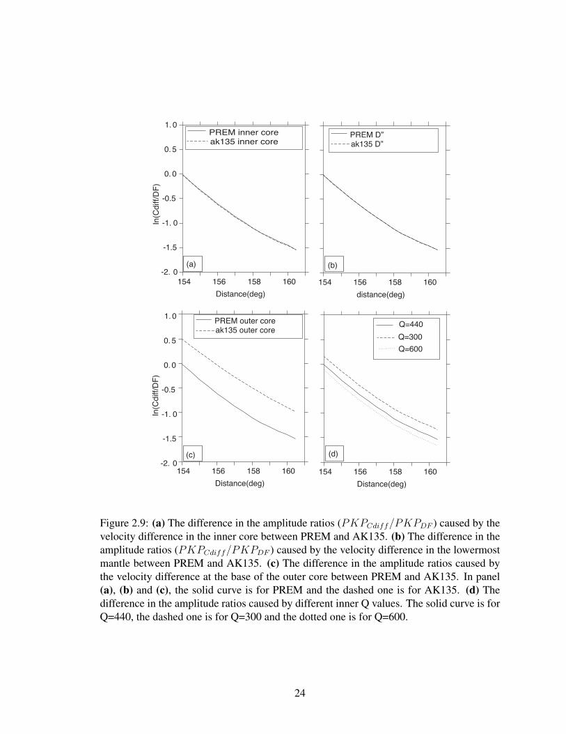
Before we evaluate the different trial models, we perform sensitivity tests to see what

Earth properties most affect PKPCdiff /PKPDF amplitude ratios. As expected, we find

that the difference in the inner core and the lowermost mantle velocity between different

reference models does not affect the amplitude ratios significantly, but that the difference

in the velocity at the base of the outer core has a very prominent effect on the amplitude

ratios (Figure 2.9). A smaller velocity gradient at the bottom of the outer core tends to

generate larger PKPCdiff amplitudes, thus larger amplitude ratios (PKPCdiff /PKPDF ).

Therefore, AK135 predicts much larger PKPCdiff /PKPDF amplitude ratios than PREM.

We also confirmed that the difference in the velocity at the base of the outer core between

PREM and AK135 has nearly no effect on the PKPDF amplitude. Thus the large amplitude

ratios from AK135 are totally due to the large PKPCdiff amplitudes. Unlike the differ-

ential travel times, however, the effect of inner core P-wave attenuation (Q) on amplitude

ratios is not negligible (Figure 2.9c). Smaller Q in the inner core decreases the PKPDF

21

PREM

AK135western hemisphere

eastern hemisphere

-2.0

-1.5

-1.0

-0.5

0.0

0.5

1.0

In(C

diff/

DF)

154 155 156 157 158 159 160 161

Distance(deg)

this study

Figure 2.8: Observed amplitude ratios of (PKPCdiff/PKPDF ). The solid curve is thepredicted amplitude ratios from PREM and the dashed curve is for AK135. The pluses arefor the data sampling the eastern hemisphere, and the gray circles are for the data samplingthe western hemisphere. The dotted curve is the synthetic amplitude ratio from the velocitymodel yielded by the amplitude ratios when inner core Q = 400 as shown in dotted curvein Figure 2.7. Both data and synthetics have been obtained from seismograms filtered witha narrow bandpass centered at 3 s.

22

amplitude, and thus increases the PKPCdiff /PKPDF amplitude ratio. Therefore, there is

always a trade-off between inner core attenuation and the velocity structure at the base of

the outer core.

We perform a similar grid search over the velocity structure at the base of the outer core

as we did for the travel times. To account for the effects of inner core attenuation, we assign

different inner core Q values (300, 400, 500, 600) for each of the velocity models. This

range is defined based on the results of several recent investigations (e.g. Dziewonski and

Anderson, 1981; Bhattacharyya et al., 1992; Wen and Niu, 2002; Cao and Romanowicz,

2004; Yu and Wen, 2006; Garcia et al., 2006). Therefore, the total number of models we

evaluate is four times those evaluated in the travel time analysis. By minimizing the L2-

norm misfit function between the observed and synthetic amplitude ratios in log-space, we

find the best fitting model.

Not surprisingly, for different values of inner core Q, we obtain different best fitting

models. However, all the models are significantly different from the best model found by

fitting the travel times. Even when we let the inner core Q be 600, the best model with

respect to the amplitude ratios still has significantly faster velocity at the base of the outer

core than the best model with respect to the differential times. For example, the dotted

line with shadowed area in Figure 2.7 shows the best fitting model and its uncertainty

obtained from bootstrap resampling algorithm with a reasonable inner core Q value of 400.

The corresponding predicted amplitude ratio curve is presented in Figure 2.8 as the dotted

curve. A smaller inner core Q value decreases the PKPDF amplitude, and thus requires a

smaller PKPCdiff amplitude, which corresponds to a steeper velocity structure. The best

model from the travel times gives too big PKPCdiff amplitudes that are inconsistent with

our observations.

We check the robustness of this result with several additional tests. Allowing for a

depth-dependent inner core Q, by using different combinations of Q in the upper 200 km

of the inner core (Q from 100 to 1000) and Q for the rest of the inner core (Q from 600

to 1000), we find PKPCdiff /PKPDF amplitude ratios for the best travel-time derived

velocity model are consistently too large compared to the observations. We find the same

result for several other high-quality velocity models determined in section 3.2. Considering

23

-2. 0

-1.5

-1. 0

-0.5

0. 0

0. 5

1. 0

In(C

diff/

DF)

154 156 158 160Distance(deg)

154 156 158 160Distance(deg)

154 156 158 160Distance(deg)

ak135 inner corePREM inner core

ak135 outer corePREM outer core

Q=300 Q=440

Q=600

(a)

(d)(c)

154 156 158 160distance(deg)

ak135 D”PREM D”

(b)

-2. 0

-1.5

-1. 0

-0.5

0. 0

0. 5

1. 0

In(C

diff/

DF)

Figure 2.9: (a) The difference in the amplitude ratios (PKPCdiff/PKPDF ) caused by thevelocity difference in the inner core between PREM and AK135. (b) The difference in theamplitude ratios (PKPCdiff/PKPDF ) caused by the velocity difference in the lowermostmantle between PREM and AK135. (c) The difference in the amplitude ratios caused bythe velocity difference at the base of the outer core between PREM and AK135. In panel(a), (b) and (c), the solid curve is for PREM and the dashed one is for AK135. (d) Thedifference in the amplitude ratios caused by different inner Q values. The solid curve is forQ=440, the dashed one is for Q=300 and the dotted one is for Q=600.

24

a frequency-dependent inner core Q model suggested previously (e.g. Li and Cormier,

2002; Cormier and Li, 2002), we experiment with lower corner frequency of 0.1-0.5 Hz

and find that they do not significantly change the amplitude ratios as well. We also find

that changes to the density jump and shear velocity jump across the ICB have relatively

small changes on the theoretical amplitude ratios, and do not allow the travel time data to

be reconciled with the amplitude data.

2.5 Discussion

Our PKPCdiff − PKPDF differential times give a flatter velocity structure at the

base of the outer core than PREM (Dziewonski and Anderson, 1981), which may imply

a different chemical composition at the base of the outer core, as suggested by previ-

ous studies (Souriau and Poupinet, 1991; Song and Helmberger, 1995). However, our

PKPCdiff /PKPDF amplitude ratios do not support this feature (Figure 2.7), instead they

prefer a PREM-type velocity structure at the base of the outer core, regardless of inner

core Q values. This apparent discrepancy is indirectly supported by many previous stud-

ies. The result from the differential times is especially consistent with those studies based

on travel times (e.g. Souriau and Poupinet, 1991; Song and Helmberger, 1995; Kennett

et al., 1995; Yu et al., 2005). Meanwhile, our result from the amplitudes ratios is con-

sistent with previous PKPCdiff amplitudes studies (Choy and Cormier, 1983; Cormier,

1981). Note that it is also consistent with the results of PREM2 (Song and Helmberger,

1995). In that study the authors found that for either constant Q or constant t? in the inner

core, the PKPCdiff /PKPDF amplitude ratios predicted by PREM2 were larger than the

observations (see Figure 8 in Song and Helmberger (1995)).

It is also important to point out that any potential bias in our data selection magnifies

the discrepancy. By choosing only waveforms with high quality PKP phases, it is possible

that our dataset is skewed towards abnormally large PKPCdiff waves. However, the best-

fitting travel time model would be inconsistent with PKPCdiff waves even larger than

what we observe. In other words, if a hypothetical perfectly averaged PKPCdiff data set

has lower amplitudes than our data set, the discrepancy with the travel times would be even

25

bigger than what we observe.

To summarize, the observed PKPCdiff amplitudes are smaller than what is expected.

This is analogous to earlier seismological studies that found unexpectedly small ampli-

tudes for Pdiff amplitudes, suggesting some sort of complexity in the lowermost mantle

(e.g. Ruff and Helmberger, 1982). In that case, the preferred interpretation of the authors

was of a jagged, but positive velocity gradient in the lowermost mantle, implying that D” is

more complicated than a simple, thermal boundary layer. However, in our case the velocity

structure just above the ICB cannot be altered to match the observed amplitudes because

the predicted travel times would then become inaccurate. Instead a non-standard mecha-

nism must exist that acts to reduce PKPCdiff amplitudes while not significantly affecting

the corresponding travel times. It appears that the small-scale heterogeneity inside the in-

ner core observed by many authors (e.g. Vidale and Earle, 2000; Cormier and Li, 2002;

Koper et al., 2004; Leyton and Koper, 2007) would not be able to explain this discrepancy

because the inner core scattering would decrease the PKPDF amplitude and thus increase

the PKPCdiff/PKPDF ratios. We believe the two primary candidates for explaining the

observed discrepancy are (1) small-scale topography or roughness on the ICB that scatters

energy from the main PKPCdiff phase into trailing coda waves, and (2) a layer at the base

of the outer core that possesses low intrinsic Q owing to anelastic mechanisms.

2.5.1 Hypothesis #1: A Rough ICB

Although strong coda waves following PKPCdiff have been observed, they are gener-

ally not interpreted as being caused by irregularities at the ICB (Nakanishi, 1990; Tanaka,

2005; Zou et al., 2007). Slowness information derived from array and polarization analysis

tends instead to support scatterer locations in the mantle. However, these studies do not ex-

clude a contribution to PKPCdiff coda waves from complexities at the ICB, and several re-

cent studies have found independent evidence favoring a rough ICB. Poupinet and Kennett

(2004) proposed inner core boundary scattering to explain the complexity of the PKiKP

coda recorded at Warramunga seismic array and suggested the ICB has some short-scale

heterogeneities with lowered wavespeed. Koper and Dombrovskaya (2005) found large

26

variation in PKiKP/P amplitude ratios and suggested the presence of heterogeneities at,

or very near the ICB. Significant variability of PKiKP amplitudes from explosion sources

also led to the suggestion of a mosaic structure at the inner core’s surface (Krasnoshchekov

et al., 2005). Most recently, high-quality earthquake doublet data recorded at different lo-

cations suggested that small-wavelength, irregular topography is present at the ICB (Wen,

2006; Cao et al., 2007).

To evaluate this hypothesis numerical simulations of short-period PKPCdiff waves

for rough ICB models need to be carried out to determine if geodynamically reasonable

structures have the desired effect. This is a difficult problem that is outside the scope of

this paper, but it is potentially feasible using modern computation approaches such as the

axi-symmetric finite difference method that has recently been used to simulate the effect

of complicated CMB models on ScS and core grazing S waves (Lay et al., 2006), or the

pseudo-spectral method recently applied to inner core scattered waves (Cormier, 2007).

A numerical evaluation is also important because of the counter-intuitive possibility that a

rough ICB would lead to enhanced PKPCdiff amplitudes, as in Biot scattering associated

with seafloor topography (Menke, 1982).

2.5.2 Hypothesis #2: A Slurry Zone at the Base of the Outer Core

In this scenario, we hypothesize that intrinsic attenuation in the lowermost outer core

is much higher compared to the rest of the outer core. Thus, the amplitude of PKPCdiff

would be significantly reduced while travelling horizontally in the low-Q layer, but PKPDF

amplitudes would be less affected because of the steeper ray paths through the layer. This

type of model has been suggested on geodynamical grounds and termed a slurry zone

(Loper and Roberts, 1978; Loper, 1978; Loper and Roberts, 1981). Such a feature could

be formed by the nucleation and gradual precipitation of solid particles from super-cooled

fluid at the base of the outer core. Alternatively, the super-cooling instability could lead to

the radial growth of dendritic arms of solid material from the inner core into the outer core,

forming a thin, mushy zone; presumably, dendrites from the mushy zone could be broken

and distributed throughout the base of the outer core by large scale convective motions

27

(Copley et al., 1970; Loper and Roberts, 1978). Internal friction between suspended solid

particles and the surrounding fluid is expected for seismic waves traversing the region, and

therefore the slurry layer might be expected to have relatively low Q compared to the rest

of the outer core.

To our knowledge, there has been only one seismic study in which such a model has

been quantitatively evaluated (Cormier, 1981). In this model (designated as QIC3) Q in-

creased smoothly from 200 to 10,000 as the radius increased from the ICB to about 250 km

shallower. QIC3 was rejected because it underpredicted absolute short-period PKPDF am-

plitudes measured at WWSSN stations (Buchbinder, 1971). However, we note that QIC3

also possessed an extremely low-Q layer at the top of the inner core, with a minimum Q

value of 125 just beneath the ICB tapering to a Q value of 1000 about 250 km beneath the

ICB.

To evaluate the possibility of a low-Q layer at the base of the outer core we carry out a

systematic grid search similar to the ones described earlier. We fix the velocity structure to

the model preferred by the PKPDF − PKPCdiff differential travel times (Figure 7) and

search over a range of Q values (from 100 to 600 with 50 as the interval) and thicknesses

(from 50 km to 400 km with 50 km as the interval) to find the parameters that best fit the

observed PKPDF /PKPCdiff amplitude ratios. Assuming an inner core Q of 400, the best

model has a Q of 300 over the bottom 350 km of the outer core. In this case, the pre-

dicted amplitude ratio curve is very close to the synthetic curve (the dotted curve in Figure

2.8) from the best model preferred by the amplitude ratios. Unfortunately, the problem is

underdetermined as there are significant trade-offs among the model parameters: between

inner core Q and outer core Q, and between outer core Q and layer thickness. However, we

do find that extremely thin (< 100 km) outer core low-Q layers are incompatible with the

amplitude ratios because they lead to overly steep decay rates.

The best-fitting models found above significantly reduce absolute PKPDF amplitudes,

although not as much as QIC3. For instance, with a Q of 300 at the bottom 350 km outer

core, PKPDF amplitude decreases by 24%, and PKPCdiff amplitude decreases by 52%

at distance of 158◦. This effect would be expected to be larger at smaller distances, as

PKPDF travel less steeply through the base of the outer core; however, the variation in

28

absolute PKPDF amplitude is on the same order predicted for models with extremely low-

Q layers at the top of the inner core and a standard outer core model.

2.6 Conclusions

We systematically searched the high-quality PKPCdiff waveforms from all the tempo-

rary networks with data currently available at IRIS DMC and some regional seismic arrays

to assemble the largest PKPCdiff data set ever. Our best model derived by fitting the dif-

ferential times (PKPCdiff − PKPDF ) indicates that the velocity and its gradient at the

base of the outer core are significantly lower than those in PREM, which is consistent with

many previous studies (e.g. Souriau and Poupinet, 1991; Song and Helmberger, 1995; Ken-

nett et al., 1995; Yu et al., 2005). The relatively low gradient at the base of the outer core

implies that the Bullen parameter is significantly greater than 1, which in turn implies the

existence of an abnormally dense layer at the base of the outer core (Souriau and Poupinet,

1991; Song and Helmberger, 1995). This may explain why recent body wave estimates of

the density jump across the ICB are smaller than estimates made from broadly sensitive

normal mode observations (Koper and Dombrovskaya, 2005).

However, our best fitting model derived from the amplitude ratios lacks the flat velocity

profile at the base of the outer core required by the travel times, and instead it is closer to

the velocity profile in PREM. This result is also consistent with some previous PKPCdiff

amplitude studies (Choy and Cormier, 1983; Cormier, 1981). We believe the velocity

profile at the base of the outer core is in fact significantly flatter than PREM, as revealed

by our travel time analysis, and that observed PKPCdiff amplitudes are reduced by a non-

standard mechanism not normally included in synthetic seismograms.

One way to reconcile our travel time and amplitude observations is with the existence of

rough topography on the ICB that acts to scatter energy away from PKPCdiff as it propa-

gates horizontally above the ICB. A complicated or rough ICB has recently been suggested

by several authors using independent data sets of waves reflected from the ICB (Poupinet

and Kennett, 2004; Koper and Dombrovskaya, 2005; Krasnoshchekov et al., 2005; Wen,

2006; Cao et al., 2007). This would be an elastic process in which energy is partitioned

29

away from the main phases into later arriving coda waves. Several researchers have exam-

ined unusual looking PKPCdiff coda waves, but to date all of the analyses have preferred

mantle locations for the scatterers. Nevertheless, the evidence from the PKiKP stud-

ies warrants the future numerical experimentation to determine if reasonable models of

ICB complexity can produce the needed reduction in PKPCdiff amplitudes, while leaving

PKPCdiff travel times relatively unchanged.

A second way to reconcile our observations is with the existence of a relatively low-Q

layer at the base of the outer core. For example, a model with flat velocities at the base

of the outer core (similar to AK135), an inner core Qp of 400, and a 350 km thick layer

with Qp of 300 at the bottom of the outer core fits both the travel time and amplitude con-

straints. Therefore, besides being unusually dense, the base of the outer core may also be

unusually attenuating at body wave periods (1-10 s). A physical model for such properties

was suggested by Loper and Roberts (1978) in the form of a slurry layer of suspended solid

Fe particles in a fluid matrix. Extrapolating results of ultrasonic attenuation experiments

with metal powder-viscous liquid suspensions (Schulitz et al., 1998) suggests that the vis-

cosity of such a slurry would be on the order of 1011 Pa s to produce the observed body

wave attenuation. Recent metallurgical studies, however, suggest that such a slurry layer

is unlikely to exist, because of the dendritic growth patterns observed in solidifying metals

(Bergman, 1997; Bergman et al., 2005). However, a recent study (Gubbins et al., 2007) re-

investigated this scenario and proposed a core model in which part of the light components

forms a solid upon freezing of the inner core, and then floats upwards and remelts at some

point. To fit the seismic properties and heat fluxes, their preferred model has a 200 km thick

layer at the base of the outer core which has less light elements concentration than the rest

of the outer core. This provides a physical explanation for the larger density gradient and

smaller velocity gradient for the bottom 200 km of the outer core, and the possible low Q

there as well.

Although bulk Q in the upper 1000 km of the outer core has been measured to be nearly

infinity from high frequency body waves (e.g. Cormier and Ricards, 1976), it is possible

there may be some deeper bulk attenuation. This idea of a low-Q layer at the base of the

fluid core can be further evaluated in two ways. First, the optimal models reported here can

30

be tested against the large databases of PKPDF /PKPAB−BC amplitude ratios that exist

at distances both smaller and larger than the range considered here (Garcia et al., 2006).

Second, the low-Q models can be tested against normal mode observations. A recent study

that used a global search algorithm to fit a large database of normal mode observations

found that existing radial Qκ models of the outer are too large by factors of 2-10 (Resovsky

et al., 2005). Those authors preferred a value of Qκ ∼ 6000 for the outer core, a value

much higher than suggested here for the base of the outer core; however, the outer core was

treated as a single layer and no allowance was made for variation within this layer. Because

the mode data averages significantly over radius, it’s possible a low-Q layer is consistent

with the data if a more flexible parametrization is used.

31

Chapter 3

Partial Melt in the Lowermost Mantle Near the

Base of a Plume

Precursors to the seismic core phase PKP have long been used to study small-scale

heterogeneities at the base of the mantle. They are preferred to PKP coda waves (postcur-

sors) because the latter are more biased by shallow structure, and so are cruder probes of

the deep Earth. In this work, however, we present an array-based analysis of PKP coda

waves that provides a unique opportunity to image small-scale structure in the deep man-

tle. Seismograms of a Peru earthquake recorded by an array of broadband seismometers

in Tibet show strong coda waves following PKPCdiff . The coda waves are strongest for

distances of 154◦ − 157◦ at frequencies above 0.5 Hz. No such strong coda waves exist

after PKPDF and PKPAB, and an empirical source time function of the earthquake is

likewise simple. This implies that the coda waves are being created by anomalous struc-

tures deep within the Earth. Using slant stack analysis we find that the ray parameter of

the PKPCdiff coda waves is similar to that of the main PKPCdiff phase, implying that the

coda waves are not simple precursors to the minimax PKPAB phase. Combined modeling

of the differential travel times, differential slownesses (PKPDF -PKPCdiff ), and envelopes

of the coda suggests that the waves are created by strong heterogeneity at the source side

of the lowermost mantle that scatters incident P energy into postcritical reflections from

the inner core boundary (P.PKPCD). Although the precise geometry is unconstrained,

if we use single scattering theory the data are consistent with a region of at least 15% P

wave velocity reduction. The most likely cause for such a strong velocity anomaly is the

presence of partial melt. The geographical location of the anomalous region, beneath the

Amazon River in South America, roughly corresponds with the expected base of a newly

discovered plume.

32

3.1 Introduction

Precursors to the core phase PKP were observed in the shadow zone as early as 1934

(Gutenberg and Richter, 1934), but debate has continued until the present on their origin

and implications. Early studies of the precursors favored the presence of a transition layer

between the outer and inner cores (Bolt, 1962; Sacks and Saa, 1969). The first challenge

to this idea came from Doornbos and Husebye’s array-based observations that the travel

times and slownesses of the precursors were inconsistent with the transition layer inter-

pretation (Doornbos and Husebye, 1972). Moreover, Cleary and Haddon (1972) showed

that the theoretical travel time curve of singly scattered waves generated by irregularities

near the core-mantle boundary (CMB) was consistent with the observations of travel time

and slowness. By adapting Chernov’s acoustic scattering theory (Chernov, 1960) to elastic

media, Haddon and Cleary (1974) first computed scattered amplitudes due to volumetric

inhomogeneities and showed that random heterogeneities of 1 per cent variation in seismic

velocity and density throughout a 200 km thick D” can explain the observed energy level

of precursors. Later computations of the amplitude of scattered waves due to an irregular

CMB topography by Doornbos (1978) indicated that a few hundred meters in height would

also produce the observed energy level, a result confirmed by Bataille and Flatte (1988).

Although it is now generally accepted that PKP precursors are generated by the scat-

tering of volumetric inhomogeneities in the mantle or CMB topography (Bataille et al.,

1990), the debate about their distribution and properties, and what they imply about the

Earth, remains active. Small-scale weak heterogeneity (1 per cent r.m.s. velocity varia-

tion) uniformly distributed throughout the mantle is supported by the modelling of PKP

precursor amplitudes (Hedlin et al., 1997). However, anomalously large PKP precursors

from earthquakes in northern Tonga indicate much stronger regional heterogeneity (10-15

per cent r.m.s. velocity variation) in a layer about 60 km thick near the CMB, support-

ing the presence of partial melt (Vidale and Hedlin, 1998). PKP precursors sampling the

ultra-low velocity zone (ULVZ) at the CMB beneath the Western Pacific also support the

presence of partial melt in a region 60 km to 80 km in height, with at least 7 per cent r.m.s.

velocity perturbation (Wen and Helmberger, 1998). However, not all heterogeneity in the

33

lower mantle is thought to be related to partial melt, for example, an analysis of PcP pre-

cursors in the North Atlantic indicating the existence of small-scale heterogeneities with

weak positive velocity anomaly in the lowermost mantle, is consistent with chemical het-

erogeneity (Brana and Helffrich, 2004).

Precursors to PKP have been frequently used to study the small-scale structure of the

deep Earth because they are not contaminated by late-arriving scattered waves created by

shallow structures. The utility of postcursors to PKP (coda waves) has also been inves-

tigated although it is a less sensitive probe for inferring mantle heterogeneity. Hedlin and

Shearer (2002) analyzed PKP recordings filtered in the bandpass from 0.7 and 2.5 Hz

at distances from 120◦ to 145◦ and concluded the existence of small-scale heterogeneities

with 1 per cent r.m.s. velocity variation throughout the lower mantle. However, the coda

arrivals did not strongly constrain the vertical distribution of heterogeneity in the mantle

because of the large standard errors of their stacked data, presumably caused by interfer-

ence with the energy scattered from shallower depth. Nakanishi (1990) observed PKPCdiff

coda waves from a deep earthquake at a seismic array in Japan and pointed out the com-

plicated frequency-dependent phenomenon of PKPCdiff coda waves. He found a slowness

of the coda waves of ∼ 4 s/deg, which is approximately equal to that of PKPAB, and

interpreted them as the scattering from the upper mantle (about 650 km). More recently,

Tanaka (2005) presented characteristics of PKPCdiff coda waves from the small-aperture

array short-period stations of the International Monitoring System. He observed wide range

of slownesses for the PKPCdiff coda waves, and interpreted the coda waves with slowness

larger than 2 s/deg as scattering from the core-mantle boundary under the source side and

receiver side, although an ICB origin could not be ruled out.

Here we present an analysis of a high quality PKPCdiff record section recorded by a

temporary array of broadband seismometers in Tibet (INDEPTH-III, International Deep

Profiling of Tibet and the Himalaya Phase III). The seismograms were generated from a

deep Peru earthquake and show enormous PKPCdiff coda waves at distances of 154.7◦ −

157◦. Combined modeling of the travel time, horizontal slowness, amplitude, and fre-

quency content of the coda waves leads to a precise estimate of the location and properties

of the anomalous Earth structure responsible for creating the coda waves.

34

3.2 Data

The INDEPTH-III array consisted of 54 broadband and short period seismometers de-

ployed from August, 1998 through May, 1999 (Figure 3.1). The stations were arranged

in a linear geometry with interstation spacing of about 10 km, and were well-positioned

to record PKP waves from earthquakes in the South America subduction zone. One

earthquake with moment magnitude 6.1 in Peru (event 981008 in Figure 3.1) in partic-

ular showed clear PKPCdiff waves followed by prominent coda waves at distances of

154.7◦ − 157◦ (Figure 3.2). For an event at this depth the C-cusp of the PKP travel

time curve occurs at approximately 152.6◦ in PREM (Dziewonski and Anderson, 1981),

and past this point geometric ray theory predicts no arrivals. However, calculations using

full wave theory show that significant diffracted energy exists well past the C-cusp, even at

relatively high frequencies (Cormier, 1981).

We selected those broadband recordings of PKPCdiff with high signal-to-noise ratio

(SNR), and applied different bandpass filtering to the waveforms. We found that the ampli-

tudes of these coda waves decrease for longer periods: they are clearly seen above 0.5 Hz

and are not seen at lower frequencies. In Figure 3.2 we present a vertical component record

section in a higher frequency passband (0.33-0.67 Hz) and a lower frequency passband

(0.067-0.133 Hz). Note that at the lower frequencies the PKPCdiff coda waves essentially

disappear and after about 157◦ the coda waves disappear even in the higher frequency band.

It is important to point out that we do not see PKPCdiff coda waves from two neighbor-

ing events (events 990302 with Mw 5.9 and 990305 with Mw 5.8) with distance ranges of

157.2◦− 159.3◦ and 156.1◦− 158.1◦, respectively, although PKPCdiff itself is clearly seen

for both of them (Figure 3.3 and Figure 3.4).

3.3 Ray Parameter of PKPCdiff Coda

In order to identify the origin of the high-frequency coda following PKPCdiff (Figure

3.2), we used a slant stack analysis. First, we aligned all of the traces with cross correlation

over the PKPDF time window. We then fixed the backazimuth at the theoretical value and

35

100 km

981008

990302

990305

-80o -60o -40o -20o 0o 20o 40o 60o 80o 100o 120o

40o

20o

0o

-20o

-40o

40o

20o

0o

-20o

-40o

-80o -60o -40o -20o 0o 20o 40o 60o 80o 100o 120o

86o 87o 88o 89o 90o 91o 92o

31o

32o

33o

34o

30o

INDEPTH-III

-10o

-5o

0o

5o

-15o

-20o

-70o -60o -50o

100 km

AR

Figure 3.1: Source-receiver geometry for the seismic data presented here. The three dotsrepresent the locations of the three events (981008: 16.12◦S, 71.40◦W, 136 km; 990305:20.42◦S, 68.96◦W, 106 km; 990302: 22.72◦S, 68.50◦W, 110 km). The solid triangle iswhere the INDEPTH-III array was deployed. The ellipse marks the region at the CMBwhere partial melt is likely to exist, and the heavy black curves represent the great circlepath (theoretically, the seismic ray path) from the events to the array. The circle with ”AR”inside is the surface location of the Atlantic ridge plume (from Montelli et al. 2004). Theupper left insert shows the detailed possible location of the partial melt at the CMB, indarker gray for PREM, lighter for PREM2, and lightest for AK135. The lower right insertshows the configuration of the INDEPTH-III array.

36

(b)

155

156

157

158

Dist

ance

(deg

)

1180 1200 1220 1240 1260 Time (s)

PKPdf PKPCdiff PKPab

1180 1200 1220 1240 1260 Time (s)

pPKPdf

pPKPCdiff

pPKPab

sPKPab

-5-4-3-2-1012345

Ray

Para

met

er (s

/deg

)

1180 1200 1220 1240 1260 Time (s)

0.00 0.25 0.50 0.75 1.00 Beam Power (sqrt scaling)

-5-4-3-2-1012345

Ray

Par

amet

er (s

/deg

)

1180 1200 1220 1240 1260 Time (s)

0.00 0.25 0.50 0.75 1.00 Beam Power (sqrt scaling)

(a)

(c) (d)

155

156

157

158

Dist

ance

(deg

)

Figure 3.2: (a) Vertical component record section at the INDEPTH-III array for the Peruearthquake (event 981008 illustrated in Fig. 1). The traces have been bandpass filtered at0.333-0.667 Hz. Theoretical arrival times for PKPDF , PKPCdiff and PKPAB in PREMare shown as dashed lines. Note the prominence of the coda waves following PKPCdiff

and their quick decay after a distance of about 157◦. (b) Same as (a) except that the wave-forms have been bandpass filtered at 0.067-0.133 Hz. Theoretical arrival times for thedepth phases pPKPDF , pPKPCdiff , pPKPAB and sPKPAB in PREM are marked asdashed lines. The PKPCdiff coda waves have disappeared, but the depth phases are moreprominent. (c) Differential slowness with respect to PKPDF in the high frequency band.The slant stack does not include the data after 157◦. The arrival at 1182 s with 0 s/deg isPKPDF , and at 1192 s with a slowness of 0.84 s/deg is PKPCdiff . The clear arrival atabout 1200 s has a similar slowness to PKPCdiff . PKPAB has slowness of about 3 s/degat 1212 s. The depth phases with similar slowness as their corresponding direct arrivalsare also shown in the figure. pPKPDF arrives at 1220 s, pPKPCdiff arrives at 1230 s andpPKPAB arrives at about 1250 s. (d) Same as (c) but for the low frequency band. Note thepoorer slowness resolution compared to the high frequency band.

37

-5-4-3-2-1012345

Ray

Par

amet

er (s

/deg

)

1180 1200 1220 1240 1260 Time (s)

Beam Power (sqrt scaling)

-5-4-3-2-1012345

Ray

Par

amet

er (s

/deg

)

1180 1200 1220 1240 1260 Time (s)

0.00 0.25 0.50 0.75 1.00 Beam Power (sqrt scaling)

157.0

158.0

159.0

Dist

ance

(deg

)

1180 1200 1220 1240 1260 Time (s)

157.0

158.0

159.0

Dist

ance

(deg

)1180 1200 1220 1240 1260

Time (s)

pPKPdf

pPKPCdiff

pPKPab

sPKPab

PKPdf PKPCdiff PKPab

0.00 0.25 0.50 0.75 1.00

(a) (b)

(c) (d)

Figure 3.3: The same as Figure 3.2 except for another South America earthquake recordedat INDEPTH-III (event 990302 in Fig. 1). From both the waveforms and the slant stackanalysis, there is a lack of energy for the PKPCdiff coda even though the PKPCdiff itselfis very strong.

38

-5-4-3-2-1012345

Ray

Par

amet

er (s

/deg

)

1180 1200 1220 1240 1260 Time (s)

Beam Power (sqrt scaling)

-5-4-3-2-1012345

Ray

Par

amet

er (s

/deg

)

1180 1200 1220 1240 1260 Time (s)

Beam Power (sqrt scaling)

156.0

157.0

158.0

Dist

ance

(deg

)

1180 1200 1220 1240 1260 Time (s)

156.0

157.0

158.0

Dist

ance

(deg

)1180 1200 1220 1240 1260

Time (s)

pPKPdf

pPKPCdiff

pPKPab

sPKPab

PKPdf PKPCdiff PKPab

0.00 0.25 0.50 0.75 1.000.00 0.25 0.50 0.75 1.00

(a)

(c) (d)

(b)

Figure 3.4: The same as Fig. 2 except for event 990305 in Fig. 1. From both the waveformsand the slant stack analysis, there is a lack of energy for the PKPCdiff coda even thoughthe PKPCdiff itself is very strong.

39

made stacks for various values of the differential ray parameter. We chose a third order

phase-weighted stack (PWS) method to reduce the incoherent noise in the array recordings

(Schimmel and Paulssen, 1997). Because of the high SNR of the data and the relatively

large aperture of the array, we have very good resolution in slowness, and the relatively

small differences in ray parameter among the PKP waves are readily apparent (Figure

3.2). The slant stack clearly shows two separate peaks for PKPCdiff and its coda above

0.5 Hz, while at low frequencies it shows a peak only at the time of PKPCdiff . Note that

the differential ray parameter of the PKPCdiff coda (0.84 s/deg) is very close to the differ-

ential ray parameter of PKPCdiff (0.94 s/deg), and much smaller than the differential ray

parameter of PKPAB ( 3.07 s/deg). This suggests that the coda waves following PKPCdiff

are not simple precursors to the minimax phase PKPAB.

To quantify the resolution of the slowness estimates we applied a bootstrap-type resam-

pling algorithm (Tichelaar and Ruff , 1989). We randomly resampled the array elements

with replacement, generating a pseudo-array with the same number of traces as the true

array. We then performed a slant stack and found the optimal arrival time and differential

ray parameter for each phase. Repeating this process 100 times, we generated a popu-

lation of pseudo-solutions that was in turn used to estimate standard errors (1σ) for the

actual solutions. The differential ray parameter of PKPDF is 0.00 ± 0.03 s/deg (since

we used PKPDF as the reference phase) and the arrival time is 1183.15 ± 0.04 s at the

array reference distance of 155.4◦. The differential ray parameter of PKPCdiff is about

0.94 ± 0.06 s/deg at a time of 1192.55 ± 0.06 s, and the differential ray parameter of the

PKPCdiff coda is 0.84± 0.06 s/deg at a time of 1198.80± 0.07 s. To test the robustness of

these results we varied the backazimuth by ±5◦ and repeated the estimation process. The

optimal differential ray parameters changed by less than 0.06 s/deg and had error bounds

similar to those described above. We also experimented with stacks created by varying the

backazimuth for a constant differential ray parameter. Using a similar bootstrap process we

estimated the backazimuth of both PKPCdiff and its coda to be 307 ± 8◦, essentially in-

distinguishable from the theoretical backazimuth of 308◦ used in making the ray parameter

estimates.

40

Nor

mal

ized

Am

plitu

de

0 2 4 6 8 10 12 14 16 18 20

ESTF

PKPDF

PKPCdiff

PKPAB

Time (s)

Figure 3.5: Comparison of waveforms of the empirical source time function (ESTF),PKPDF , PKPCdiff , and PKPAB for event 981008. All the waveforms have been filteredat 0.667-1.333 Hz. Only PKPCdiff has a prominent coda.

3.4 The Origin of the PKPCdiff Coda

To rule out the possibility that the PKPCdiff coda waves are due to source complexity,

we obtained an empirical source time function (ESTF) using the first eigen-image tech-

nique (Ulrych et al., 1999) on 15 teleseismic (63◦ − 70◦) recordings with high SNRs. The

first eigen-image represents the most coherent signal from trace to trace and so it is a good

estimate of the source time function after excluding later phases (Bostock and Rondenay,

1999). We found a relatively simple ESTF for the event and no prominent energy within

10 s of the first arrival. As a comparison, we stacked all the traces after aligning them ac-

cording to PKPDF , PKPCdiff , and PKPAB, respectively. Comparing the four waveforms,

only PKPCdiff shows a prominent coda (Figure 3.5). Therefore the PKPCdiff coda is not

due to source complexity, and is unrelated to heterogeneity near the source or the receivers.

We also note that convolving the ESTF with a synthetic record section calculated by full

wave theory (Cormier and Richards, 1988) for a radial Earth model does a good job of

reproducing the observed PKP phases, excepting the anomalous coda waves (Figure 3.6).

We investigated the origin of the PKPCdiff coda using ray theory (therefore we restrict

the modeling to high frequencies) to compute the travel time, amplitude, and slowness

41

155.0

156.0

157.0

158.0

Dis

tanc

e (d

eg)

1170 1180 1190 1200 1210 1220 1230

T ime (s )

(b)

155.0

156.0

157.0

158.0

Dis

tanc

e (d

eg)

1170 1180 1190 1200 1210 1220 1230

T ime (s )

(a)

Figure 3.6: Comparison between (a) synthetic seismograms calculated by full wave theoryin PREM and (b) the real data for event 981008. Both synthetic and observed seismogramsare filtered around 2 s. We obtain the synthetic seismogram by convolving the syntheticsobtained from full wave theory with the empirical source time function (ESTF) presentedin Figure 3.3. No depth phases are included in the synthetic seismograms.

of waves scattered inside the Earth from various hypothetical locations. The basic idea

is to consider potential point scatterers in a region, propagate a down-going ray from the

source to each scatterer, and then propagate an up-going ray from each scatterer to the

receiver. In general the ray parameter changes after the ray interacts with the scatterer,

and we determined appropriate values to reach the receiver using pre-computed lookup

tables relating depth, distance, and ray parameter, that were calculated for a spherical Earth

model PREM (Dziewonski and Anderson, 1981). Given the appropriate ray parameter, we

calculated the travel time and the amplitude by numerically integrating the corresponding

expressions (Cerveny, 2001), which include the attenuation and geometrical spreading. We

tested various schemes and found that use of the trapezoid rule with a step of 0.1 km gave

accurate results. We accounted for the amplitude variations in the down-going rays induced

by the radiation pattern of the earthquake using standard relations (Aki and Richards, 2002)

and the Harvard CMT solution (see www.seismology.harvard.edu/CMT).

The change in amplitude during the scattering process can be estimated by using an

equivalent reflection coefficient, obtained from the propagation of an elastic wave in a

42

heterogeneous medium (Wu and Aki, 1985a,b):

gPP (θ) =2(ω/α0)

4a3(δα/α0)2(cos θ + 1

3+ 2

3cos2 θ)2

(1 + 4(ω2/α20)a

2 sin2(θ/2))2, (3.1)

where θ is the scattering angle, ω is the angular frequency, a is correlation distance, α0 is

the background medium velocity, and δα is the P wave velocity variation in the heteroge-

nous medium. Here we have assumed an exponential autocorrelation function, which is

commonly made in modeling crustal heterogeneity (Sato and Fehler, 1998). Continuing to

consider only the relative amplitude variation among hypothetical scattered waves, we held

all the variables on the right-hand-side of equation (1) constant, and calculated gPP based

on the value of θ that was appropriate for the change in ray parameter. In practice, this

amplitude variation is small because our particular geometry is close to forward scattering

(θ ≈ 14◦), but we nevertheless included it in our calculations. Finally, we projected the

amplitude of the resulting up-going wave in the vertical direction and accounted for the

free surface effect (Cerveny, 2001).

We computed the effect of a volumetric scattering by ray-tracing for the rays that leave

the source to the scattering region (pre-scattering). Then, they interact with the scatterer

by means of the apparent reflection coefficient mentioned before. Finally, we send the rays

towards the receiver through the post-scattering ray (also using ray-tracing techniques). In

Figure 3.7 we present the results of these calculations assuming that the causative scat-

terer is located just above the CMB and somewhere along the great circle path (i.e., in the

sagittal plane). The scatterer produces 4 new core phases: P.PKPDF , P.PKPCD, and

P.PKPBC in analogy with the normal PKP branches (Figure 3.7a), as well as a retro-

grade version of P.PKPDF , which is not presented in Figure 3.7. There are significant

differences in the relative amplitudes of the scattered waves, with the postcritical reflec-

tion from the ICB (P.PKPCD) being the largest (Figure 3.7b). By matching the observed

P.PKPCD − PKPDF differential travel time with our numerical predictions we find a

unique location for the scatterer, that also predicts a P.PKPCD − PKPDF differential ray

parameter that matches our observations (Figure 3.7c). This interpretation is supported by

43

two additional observations. First, for our source-receiver geometry, P.PKPCD only exists

to a distance of 156◦ − 158◦; afterwards it begins to diffract and quickly loses energy. The

precise distance of the cusp depends somewhat on the assumed reference Earth model. This

then explains the sudden decrease of the observed PKPCdiff coda waves past about 157◦

(Figure 3.2), as well as the lack of significant PKPCdiff coda waves for two neighboring

earthquakes that generated PKP waves across the INDEPTH-III array at slightly larger

distances (Figure 3.3 and Figure 3.4), although it is also possibly because they sample

slightly different area at the CMB. Second, note that the PKPCdiff coda wave has a shape

much more similar to PKPAB than the other pulses. PKPAB passes through a caustic and

so picks up a phase shift of 90◦ (Hilbert transform) with respect to the source pulse. It is

expected that P.PKPCD, being a post-critical reflection, would have a significant phase

shift as well, and in fact the computed value is 83◦.

Under the above assumptions, the geographical location of the scattering region is about

20◦ from the epicenter, roughly at 0.2◦S and 56.9◦W, beneath the Amazon basin. The pre-

cise distance along the great circle path depends on the assumed 1D reference model, and

the distance off the great circle path is bounded by the observed uncertainties in the back-

azimuth of P.PKPCD. These constraints define an annular segment just above the CMB

as shown by the ellipse in Figure 3.1. Unfortunately, there is still a trade-off involving the

exact depth of the scattering region. For instance, the differential travel time and slowness

observations of P.PKPCD can be equally well explained by placing the scattering region

simultaneously at shallower depths (up to about 1100 km above the CMB) and smaller

epicentral distances (down to 10◦). However, we are confident that the scattering region is

indeed located on the source side of the lower mantle. Any location on the receiver side

of the lower mantle will produce large differential ray parameters at the appropriate time.

Placing the heterogeneity at the inner core boundary would require a P wave to travel for

almost 60◦ as a diffracted wave in order to arrive at the receiver with the appropriate time

as in the data. In this case, the energy (especially the higher frequency contents) would be

strongly attenuated, which is inconsistent with our observations. Locating the scatterer in

the upper mantle would lead to the appearance of scattered phases after every direct PKP

arrival, again inconsistent with our observations.

44

020

40

6080 100 120

140160

180

PKPDFP.PKPDFP.PKPCDP.PKPBC

(a)

(b)

(c)

Diff

eren

tial R

ayPa

ram

eter

(s/d

eg)

Rel

ativ

e Am

plitu

de

Time Relative to PKPDF (s)

0

1

2

3

0 10 20 30 40 50 60 70

10-5

10-4

10-3

Figure 3.7: Properties of the geometrical scattered waves that result from a heterogeneitylocated at the CMB, 20◦ from the source: (a) ray paths of the direct arrival of PKPDF

(black full line) and 3 scattered waves (green for P.PKPDF , blue for P.PKPCD, andred for P.PKPBC); (b) Relative amplitude with respect to PKPDF by assuming both thevelocity perturbation and scattering volume are 1; and (c) their differential ray parameterwith respect to PKPDF (following the same color code). The dashed black lines in thetwo lower panels show the differential time and differential ray parameter observed for thePKPCdiff coda, corresponding to the scatterer position shown in (a).

45

Further insight on the nature of the scattering region can be gained by considering

the relative amplitude of P.PKPCD. Assuming a random inhomogeneous medium and

the single scattering approximation (Wu and Aki, 1985a; Cormier, 1995), the directional

scattering coefficient, gPP , is related to the observed scattered wave amplitude, A, by:

(A

A0

)2

=V gPP (θ)

G(r)(3.2)

where G(r) is the geometric spreading with r as the total traveled distance, V is the scat-

tering volume, and A0 is the amplitude of the incident wave. In our case, the scattering

angle, θ, is about 14◦, the correlation distance, a, is about 10 km and the angular frequency

is 2π. The geometrical spreading factor, G(r), is obtained from the usual ray techniques

(Cerveny, 2001). Plugging in these values, equation (2) can be combined with equation

(1) to yield a relationship with just 2 free parameters: the scattering volume V and the

r.m.s. P wave velocity contrast δα/α0. To remove uncertainties in the source and re-

ceiver effect, as well as the instrument response, we computed the amplitude ratio between

P.PKPCD and PKPDF . At an epicentral distance of 156◦, the observed amplitude ratio

between P.PKPCD and PKPDF is about 0.43 and corresponding theoretical amplitude

ratio is 4.309 × 10−4(δα/α0)2V with V and δα/α0 unknown. Equating the observed and

theoretical values we get an implicit relation between V and δα/α0 (Figure 3.8a).

Based solely on Wu and Aki’s work (Wu and Aki, 1985a,b), there is always trade-off

between the scattering volume and the velocity perturbation: a bigger scattering volume

needs a smaller velocity perturbation to generate the same amplitude of the scattered wave;

however, a large scattering volume should lead to a relatively long wave train of coda. For

a small region, only a few rays will be able to sample it producing a smaller duration of the

coda wave. Using a trial-and-error method, we computed synthetic envelopes for different

suitable combinations of scattering volume and velocity perturbation, by considering all

the possible down-going rays that were able to reach the heterogeneous medium and then

arrive at the station. We assumed a cylindrical shape for the scattering region, and con-

volved in the ESTF with each terminal arrival before taking the envelope. Comparing the

46

0.0

0.2

0.4

0.6

0.8

1.0

12 13 14 15 16 17 18 19 20

Time After PKPDF (s)

Nor

mal

ized

Am

plitu

de

(b)

1e+07

1e+08

0.05 0.10 0.15 0.20 0.25 0.30 0.35 0.40Fractional Velocity Perturbation

Volu

me

(km

3 )

(a)

Figure 3.8: (a) Trade-off between scattering volume and fractional velocity perturbation.The black curve represents all possible volume-perturbation pairs that generate the ob-served amplitude of P.PKPCD. The red, pink, green, and blue stars mark the positionwith 6%, 18%, 22%, and 31% P wave velocity perturbation, respectively. (b) Compar-ison between envelopes of PKPCdiff coda of data and synthetics generated for differentvolume-perturbation pairs. The black dashed line represents the real data, while the red,purple, green, and blue lines represent the synthetics for various levels of P wave velocityperturbation. The amplitudes are normalized to the maximum.The colors are consistentwith those used in (a).

47

synthetic envelopes with the data (Figure 3.8b), our best estimate of the velocity perturba-

tion is about 18-31%, corresponding to an equivalent radius of ∼ 150 km, if we imagine

that the scattering volume is a cylinder with equal radius and height. It is important to point

out that the way we calculate the synthetic envelopes is very rough since we do not know

the shape of the anomalous region. However, under the single scattering theory, we believe

the anomaly is very strong, with P wave velocity perturbation at least ∼15%.

3.5 Conclusions and Discussion

The magnitude of the velocity perturbation we infer is too large to be explained by

chemical heterogeneity, and instead requires the existence of partial melt (Williams and

Garnero, 1996). Furthermore, because at high pressure silicate melt is denser that the

surrounding solid matrix (Rigden et al., 1989), it is unlikely that the scattering region we

observe could exist anywhere except near the CMB. Here it has been suggested that dense

partial melt raining down from above may be trapped by cumulus crystal growth (Rost

et al., 2005). Partial melt at the CMB can also be caused by other means, such as enhanced

heat flux from the core or viscous heating (Steinbach and Yuen, 1997, 1999), and its ex-

istence has been confirmed by experimental high pressure studies (Holland and Ahrens,

1997; Zerr et al., 1998). Hence, our preferred model is a partially molten region in the

lowermost mantle beneath the Amazon River basin with a P wave velocity reduction of at

least∼15%. The precise shape of the region is virtually unconstrained, and it could be thin

and broad in analogy with previously documented ULVZs.

The location of the scattering region found in this study (0.2◦S and 56.9◦W) is close to

the newly discovered Atlantic Ridge plume (Montelli et al., 2004) at 12◦N, 45◦W. In that

study, finite-frequency tomography results indicated the existence of a plume to a depth

of at least 1900 km, however resolution was lost at deeper depths. And their 3-D image

showed the plume tilted toward the south-west as it goes deeper (see Fig.S1 in their online

supplemental material). Because the plume is rising in the convective mantle, it is ex-

pected that the plume may be tilted by the “mantle wind” on its way up (Olson and Singer,

48

1985). Global mantle convection models predict that the plume root can be offset hori-

zontally more than 1000 km away from its surface location (Steinberger and O’Connell,

1998). Therefore, the Atlantic Ridge plume may actually originate at the CMB beneath the

Amazon River basin, and tilt toward the north-east while it rises. A recent S-wave tomo-

graphic study (Montelli et al., 2006) confirmed its tilt direction (see their Fig.15), which is

consistent with the result from P-wave tomography. Although no surface hot spot fed by

this plume has been reported, a suggestion about an axial hot spot around this area has been

made (Sleep, 2002).

This interpretation is consistent with similar seismic findings (Garnero et al., 1998),

suggesting a link between extreme heterogeneity at the base of the mantle and upwelling

plumes. For example, partial melt inferred to exist at the CMB north of Tonga (Vidale and

Hedlin, 1998; Wen and Helmberger, 1998) is located very near the base of the tomograph-

ically imaged Samoa plume (Montelli et al., 2004). Likewise, partial melt inferred to exist

at the CMB east of Australia is probably related to a trio of plumes near Tasmania (Rost

et al., 2005). On a more general global scale, there is a statistically significant correla-

tion between ULVZs at the CMB and hot spot surface locations (Williams et al., 1998).

Therefore, it may be common for partial melt to exist in the lower mantle near the base of

upwelling, thermal plumes.

49

Chapter 4

Using PKP Precursors Recorded at IMS Arrays

to Determine the Small-scale Heterogeneity in

the Mantle

It has been known that PKP precursors are direct evidence for the existence of small-

scale, non-radially symmetric structure in the Earth’s deep mantle since their re-interpretation

in the 1970s. However, the scattering intensity, radial, and lateral distribution of the small-

scale heterogeneities remain elusive. There are two possible reasons for the inconsistent

results reported so far. One is related to the data used in different studies. Due to uneven

data sampling and different data processing schemes, different authors may obtain different

PKP precursor envelopes. The other possible reason may be related to differences in for-

ward modeling methods. For the same data set, single-scattering theory may yield different

results for heterogeneity strength than a multiple-scattering or diffusion-based theory. In

this study, we take advantage of the globally distributed International Monitoring System

(IMS) seismic arrays to assemble a large, geographically diverse dataset of PKP precursor

envelopes. An advantage of using IMS arrays over single stations is that the recordings of

all elements at one array can be coherently stacked to suppress noise, and thus provide high

signal-to-noise (SNR) ratio PKP precursors, even for relatively small earthquakes. The

average precursor amplitudes exhibit a steady increase with time and distance. We find that

random heterogeneities with a scale-length of 8 km with 0.05% r.m.s. velocity perturba-

tion uniformly distributed throughout the lower mantle can provide a reasonable fit to the

observations. On the contrary, confining the heterogeneities near the CMB or in the D”

layer does not yield the amplitude versus time pattern observed in our data. Extra scatter-

ing near the CMB or in D” is not justified from our data. We also find that the precursors’

amplitudes vary from place to place. Some places such as off-shore of South America, the

50

southern part of the Atlantic Ocean, and central America, have weaker or similar precur-

sors compared to the average precursor. The distribution of stronger precursor amplitudes

is scattered. Even within a small geographic region, such as North America, the precursor

amplitudes exhibit small-scale lateral variations. This imples that the lower mantle is not

perfectly mixed by mantle convection and subducted oceanic lithosphere or other chemical

impurities can survive in the mantle for billions of years.

4.1 Introduction

With the increasing high-quality seismic data and the improvements of seismic imaging

techniques, we are obtaining a more and more detailed image of the Earth’s interior. Not

only is the radial seismic velocity structure well determined, but the non-radial large-scale

heterogeneities have also been revealed, such as penetrating slabs and upwelling plumes.

These findings are very important to understand mantle dynamics. Most of the discoveries

are achieved by analyzing travel times and waveforms of the main seismic phases through

tomography. However, resolving small-scale heterogeneity (with a scale length of 5-10 km)

in the deep Earth is beyond the resolution of traditional seismic tomography because of

spatial aliasing and contamination of the scattered waves by the strong heterogeneity in the

upper part of the mantle.

High-frequency coda waves following P or S wave are the direct evidence for small-

scale random heterogeneity in the Earth. Aki (1969) first showed that the scattered coda

waves, which used to be treated as noise, can be used to estimate the strength of the random

heterogeneity. Observations of PKP precursors concluded that small-scale heterogeneity

must also exist in the deep mantle (Doornbos and Husebye, 1972; Cleary and Haddon,

1972). In order to obtain a fine image of the small-scale heterogeneity, which would lead

to better understand mantle dynamics, we must carefully analyze high-frequency scattered

waves.

PKP precursors have unique advantages in studying the deep Earth scatterers, as they

are not contaminated by the direct arrivals and later-arriving scattered waves created by

shallow structure. The sharp velocity decrease from the mantle to the core causes a P -wave

51

shadow zone at 105◦-143◦ (Oldham, 1906) and the first arrival is the PKP wave refracted

in the inner core (Lehmann, 1936). Geometrical ray theory predicts no arrivals before

PKP for a radially symmetric Earth model. However, when non-radial small-scale het-

erogeneities exist in the lower mantle, scattered energy from the outer core phase (PKPab

or PKPbc) can arrive up to 18 s earlier than PKP in the range of 120◦ − 143◦ (Figure

4.1). This type of scattered energy preceding PKP was first observed in 1934 (Gutenberg

and Richter, 1934). Older studies of the PKP precursors had controversy about their ori-

gin, including refraction in the inner core (Gutenberg, 1957), refraction or reflection in a

transition layer between the outer and inner cores (Bolt, 1962; Sacks and Saa, 1969), and

diffraction from the CMB (Bullen and Burke-Gaffney, 1958). However, it is now widely

accepted that PKP precursors are generated by the scattering from volumetric inhomo-

geneities near the CMB or within the lower mantle, or from CMB topography (Doornbos

and Husebye, 1972; Cleary and Haddon, 1972; Bataille et al., 1990).

Since Cleary and Haddon (1972) showed that the precursors’ travel times were con-

sistent with those of singlely scattered waves from irregularities near the CMB, numerous

authors have focused on the scatterers’ locations, their radial and lateral variations, and their

magnitude. Several studies investigated PKP precursors recorded at some particular loca-

tions and inferred anomalously strong heterogeneities in the lowermost mantle underneath

the source or receiver side (e.g. Vidale and Hedlin, 1998; Wen and Helmberger, 1998; Wen,

2000; Niu and Wen, 2001b). Vidale and Hedlin (1998) observed anomalously large PKP

precursors from earthquakes in northern Tonga and infered 10 − 15% r.m.s. velocity vari-

ation in a layer about 60 km thick near the CMB, supporting the presence of partial melt.

By using short and long period PKP precursors, Wen and Helmberger (1998) also found

evidence for the partial melt in a region 60-80 km in height, with at least 7% r.m.s. veloc-

ity perturbation beneath the Western Pacific. A few studies concentrated on modeling the

time- and distance-dependent amplitudes of global average PKP precursors using single

or multiple scattering theory (e.g. Hedlin et al., 1997; Shearer et al., 1998; Cormier, 1999;

Hedlin and Shearer, 2000; Margerin and Nolet, 2003b). Hedlin et al. (1997) modeled

the globally averaged PKP precursors using single-scattering theory and found the best

model to fit the observations has ∼ 1% r.m.s. velocity heterogeneity at a 8 km scale length

52

0 20 

40 

60 

80 100 

120 

140 

160 

180 

S

R

0 20 

40 

60 

80 100 

120 

140 

160 

180 

S

R

(b)

(a)

850

860

870

880

890

900

910

920

930

940

950

Tim

e-2.

0*di

stan

ce(s

)

110 120 130 140 150 160 170Distance(deg)

CD

FB

A

(c)

Figure 4.1: Ray paths and reduced travel time curves for the core phases and precursors. (a)The ray path for PKIKP (black curve) and two PKP precursors (red curves) at 135◦ fora receiver side scatterer (red star) at the CMB. (b) Same as (a), but for a scatterer locatedbeneath the source side. (c) The solid curve is the standard PKP travel time curve inPREM, the dashed curve is the earliest precursor time when the scatterer is at the CMB,and the dotted curve is the earliest precursor time when the scatterer is 900 km above theCMB.

53

throughout the lower mantle. Using a revised single-scattering theory (Cormier, 1995) al-

lowing for arbitrary levels of velocity and density perturbations, Cormier (1999) confirmed

this conclusion by modeling the same dataset processed by Hedlin et al. (1997). However,

by rejecting seismograms with no clear indications of PKP precursors in Hedlin et al.

(1997)’s dataset and adding new ones from new deep events, Margerin and Nolet (2003a)

used radiative transfer theory (Margerin and Nolet, 2003b) to model precursor envelopes

and favored whole-mantle scattering with 0.1− 0.2% velocity perturbations.

The basic mechanism of generating PKP precursors is now fairly well understood,

however, the radial and lateral distributions, and magnitude of the small-scale mantle het-

erogeneity are still not fully resolved. Modeling of global average precursors tends to favor

the whole mantle scattering model instead of confining the heterogeneity near the CMB.

However, the magnitude of P -wave velocity perturbation is as much as 10 times differ-

ent among different studies. The discrepancy comes from two possible causes. One is the

dataset used in different studies. Due to uneven data sampling and different data processing

schemes, different authors may obtain different global average PKP precursor envelopes.

The other possible reason relates to differences in forward modeling theory. For the same

precursors, single-scattering theory may yield different magnitudes of heterogeneity than a

multiple-scattering or diffusion based theory. It is interesting to note that Margerin and No-

let (2003b) only selected those seismograms with strong precursors and obtained a velocity

perturbation one order of magnitude smaller than that of Hedlin et al. (1997), who included

data without strong precursors. Under the same forward modeling theory, Margerin and

Nolet (2003b) are expected to obtain larger velocity perturbation than Hedlin et al. (1997).

Therefore, a potential cause for the discrepancy is a difference between the single-scattering

theory and transport theory. However, in another manuscript, Margerin and Nolet (2003a)

showed that single-scattering and transport theories are essentially equivalent for pertur-

bations less than 0.5%, and for large perturbations (1% or more), the two theories yield

significantly different results. Since Margerin and Nolet (2003b) obtained 0.1 − 0.2% ve-

locity perturbation, the scattering theories cannot explain the discrepancy. Therefore, the

possibility that they obtained different average precursor envelopes due to using different

data processing schemes cannot be excluded. With respect to the lateral variations of small-

54

scale mantle heterogeneity, there is only one complete study which was devoted to mapping

out the large-scale variations (Hedlin and Shearer, 2000), while several individual studies

inferred very strong heterogeneity near the CMB at some particular geographic locations

(Vidale and Hedlin, 1998; Wen and Helmberger, 1998; Wen, 2000; Niu and Wen, 2001b).

In this study, we assemble a large, geographically diverse data set of PKP precursor

envelopes by using the globally distributed international monitoring system (IMS) seis-

mic arrays. An advantage of using arrays over single stations is that the recordings of all

elements at one array can be coherently stacked to suppress noise, and thus obtain high

signal-to-noise (SNR) ratio PKP precursors, even for relatively small earthquakes. We

then apply a Monte Carlo seismic phonon method to model the global averaged PKP pre-

cursor envelopes to define the small-scale heterogeneity scattering model in the mantle.

Lateral variations of small-scale heterogeneity will be discussed to better understand its

distribution and nature.

4.2 Data Processing

The mission of the International Monitoring System (IMS) is to monitor the world

for nuclear tests. A large portion of IMS seismic stations are small aperture arrays (with

aperture from 4-25 km) equipped with 10-20 short-period vertical component seismometers

in each array. Most of the IMS seismic data before December 2003 are freely available

from the U. S. Army Space and Missile Defense Command (SMDC) Monitoring Research

Program (MRP) website. Data from IMS arrays within the U.S., including PDAR, TXAR,

ILAR and NVAR, are available from May 2000 until present at IRIS DMC. Continuous

seismic data from the Yellowknife array (YKA) since 1989 can be requested from Canadian

National Data Centre (CNDC) through AutoDRM. We searched the global CMT catalog to

find the events at source-receiver distance between 120◦ and 145◦ with moment magnitude

greater than 4.5 for each IMS array during the open time period. We checked over 9000

events recorded at 11 IMS seismic arrays in the proper distance range. For each event, the

seismograms were visually inspected for the quality. We selected those events which have

clear and impulsive PKP waves and high SNRs, regardless of precursor amplitudes. For

55

each good event, the obviously noisy or glitchy traces are removed. A total of 2,223 events

(over 30,000 traces) recorded at 11 seismic arrays are selected for subseqent processing

and analysis. Table 4.1 lists the properties of all the IMS arrays used in this study and the

number of events selected for each array. Figure 4.2 shows the locations of the 11 IMS

arrays and the entry and exit points at the CMB of PKP waves under the receiver and

source sides of the selected events.

Table 4.1: IMS seismic arrays used and the number of events selected

Seismic Lat Lon Number of Aperturea EventsArray ◦N ◦E Elements km Selected

ARCES 69.535 25.506 23 3.7 247ASAR -23.665 133.951 19 9.8 216CMAR 18.420 98.959 18 11.0 91ESDC 39.671 -3.946 19 9.4 32

GERES 48.837 13.702 25 4.1 240KSAR 37.447 127.894 19 10.8 40NVAR 38.429 -118.303 11 9.9 171PDAR 42.777 -109.583 13 3.4 285TXAR 29.334 -103.667 9 4.5 572WRA -19.767 134.393 20 23.9 114YKA 62.606 -114.605 18 24.2 215

a We use the definition from Koper et al. (2003) as the diameter of the circle that has thesame area as the smallest rectangle that includes all the elements.

To determine the global average precursor amplitudes, we process the data in the fol-

lowing four steps.

First, for each event, we bandpass filter the seismograms between 0.7 and 2.5 Hz since

the dominant frequency of the precursor is 1-2 Hz. This frequency band can resolve small-

scale heterogeneities with a scale length of about 5-10 km.

Second, instead of calculating envelope functions of individual traces, as in previous

precursor studies which used data from single stations, we apply the sliding window, time-

domain beamforming to the seismograms recorded at the array to obtain the amplitude

maximum, slowness, back azimuth and coherence versus the lapse time (Koper, 2005),

which is equivalent to the sliding window frequency-wavenumber (fk) analysis developed

56

-60˚

-30˚

0˚

30˚

60˚

YKA

WRAASAR

CMAR

ESDCKSAR PDAR

TXAR

ARCES

GERES

NVAR

Figure 4.2: Locations of the 11 IMS arrays and the PKIKP entry and exit points at theCMB. Black triangles are IMS arrays. Circles and pluses are the entry and exit points ofPKIKP at the CMB under the receiver side and source side.

by Rost and Weber (2001). For a short time window with a fixed length of 1 s, we perform a

grid search over all the possible slowness and back azimuth combinations to find the ampli-

tude maximum. Then the fixed-length short time window is shifted along the seismograms

with a constant step of 0.2 s, and we perform the same grid search for the best combina-

tion of slowness and azimuth. At each step, the power maximum, slowness, back azimuth

and coherence are stored as time series. The sliding window beamforming instead of the

simple beamforming at a fixed slowness (PKP slowness) is selected because the simple

beamforming may under-estimate the precursor’s amplitude due to its different slowness

from PKP . The choices of the 1 s search time window and the 0.2 s shift step are based

on the dominant period of the precursors and the size of the seismic arrays. The precursor

has a dominant period of 0.5-1 s, so the time window should be long enough to include the

complete signals across the array for a particular phase, while being short enough to avoid

multiple phases with different slownesses appearing in the same time window, causing the

ambiguity of identifying a single phase . In this manner, we obtain a high SNR and accu-

rate estimate of PKP precursor’s amplitude for each event, which has much higher quality

than the recording at one single station. Figure 4.3 shows an example of this type of sliding

window beamforming analysis for an event recorded at the YKA array.

57

136.52

136.54

136.56

136.58

136.60

136.62

136.64

136.66

136.68

136.70

136.72

136.74

Dis

tanc

e

1120 1130 1140 1150 1160 1170 Time (s)

0.00.20.40.60.81.0

Coh

eren

ce

1120 1130 1140 1150 1160 1170 Time (s)

10 1

10 2

Bea

m P

ower

05

1015202530

Slo

wne

ss (s

/deg

) 060

120180240300360

BAZ(

deg)PKPPrecursor

Figure 4.3: Vertical record section of an example event and its sliding window slownessanalysis. (Left) Vertical component record section for an event with moment magnitude5.3 at 82.8 km depth recorded at the YKA array. The seismograms have been bandpassedat 0.7-2.5 Hz with a 3-pole Butterworth filter. PKP waves arrive at about 1152 s andprecursors can be clearly seen in the ∼ 10 s time window before PKP . (Right) From topto bottom are the back-azimuth, slowness, power and coherence measured from the slidingwindow algorithm. Precursory energy is clearly seen from the beam power plot about 10 sbefore PKP . In the same time window, the back-azimuth and slowness are stable, and thecoherence is higher than the background noise.

58

The third step of our data processing is that we apply a smoothing algorithm with width

of 1 s (5 points) to smooth the power function (we use the term envelope to refer to it for

simplicity, although it is slightly different from the common definition of an envelope) of

each event obtained at the second step. For the smoothed envelope, we search for the peak

amplitude within a time window of ± 5 s w.r.t. the predicted PKP arrival time in AK135

Earth model. Then we use the time corresponding to the peak amplitude as a reference and

search for the first local maximum with amplitude ≥ 60% of the global maximum ampli-

tude. If there is a local maximum within this criteria, we use the time corresponding to the

local maximum as the actual PKP peak arrival time. Otherwise, we use the time corre-

sponding to the global maximum amplitude as the actual PKP peak arrival time. 60% is

selected to do this search to find the actual PKP peak arrival time based on the following

two considerations. First, the precursor’s amplitude is usually less than 50% of the ampli-

tude of PKP wave from previous studies (Hedlin et al., 1997; Bataille and Flatte, 1988)

and we do not observe any precursor with amplitude greater than that either. Therefore,

using 60% as the criterion permits us to find the PKP time instead of the precursor time.

Secondly, PKiKP arriving a little after PKIKP sometimes may have bigger amplitude

than PKIKP although the predicted amplitude ratio between PKIKP and PKiKP is

around 1 (Cao et al., 2007). In this case, the global maximum amplitude may correspond

to PKiKP . Therefore, searching for the first local maximum can enable us to find the

PKIKP arrival time we intend to use as the reference for stacking. Finally, for the shal-

low events, the depth phase pPKP arriving a few seconds after PKP sometimes has

slightly larger amplitude than PKP , although the ray path and radiation pattern coefficient

are very close for the two phases. Thus, searching for the first local maximum gives us a

better chance to find the PKP time instead of pPKP arrival time.

Finally, we use a 20 s time window starting from 45 s before PKP to estimate the

noise level. SNR is defined to be the ratio between the PKP peak amplitude and the noise

level. We then subtract the noise level from the envelope function and stack the envelopes

from different events with SNR ≥ 10 in 1◦ distance bins after aligning and normalizing the

envelope functions according to the estimated PKP peak arrival time and amplitude. The

stacked global average precursors’ amplitudes increase with time and distance as shown in

59

Figure 4.4.

To test the robustness of our average precursors’ amplitudes, we took a random half of

our data set and applied the same stacking method, which yields a very similar result as the

whole data set. It is important to note that within each 1◦ distance bin, PKP precursors’

amplitudes exhibit a lot of variation from event to event. This will be discussed later.

4.3 Modeling Global Average PKP Precursor Envelopes

To model the scattering of random heterogeneity in the Earth, both single-scattering

and multiple-scattering theories have been used to compute the synthetic scattered waves’

envelopes (for a review, see Sato and Fehler (1998)). When the velocity and density per-

turbations of the heterogeneity are much weaker than those of background media, the Born

approximation is valid and single-scattering theory may be sufficient to model the scatter-

ing phenomenon. Otherwise, a multiple-scattering approach is necessary to simulate the

scattered wave field. Most multiple-scattering approaches are based on radiative transfer

theory (Wu and Aki, 1985a,b; Sato and Fehler, 1998; Margerin and Nolet, 2003a). By

using the Monte Carlo simulation based on radiative transfer theory, Margerin and Nolet

(2003a) found that the Born approximation is only valid for the r.m.s velocity perturbation

≤ 0.5%.

In this study, we use a particle-based Monte Carlo method developed by Shearer and

Earle (2004) to model the globally averaged PKP precursor amplitude. In this particle-

based simulation, millions of particles (seismic phonons) are sprayed from the source,

which are randomly scattered using probabilities computed from random media theories

(Shearer and Earle, 2004). In this algorithm, the multiple-scattering is naturally imple-

mented and intrinsic attenuation is included. We apply the seismic phonon method to a

standard Earth model PREM with random heterogeneities at different depth ranges in the

mantle. We assume an exponential autocorrelation function for the random media with

variable scale-length and r.m.s. velocity perturbation to model the observed globally aver-

aged PKP precursor envelopes.

Since only a small fraction of precursors are affected by upper mantle scattering (Figure

60

125

126

127

128

129

130

131

132

133

134

135

136

137

138

139

140

141

142

143

144

Distance(Deg)

-30 -25 -20 -15 -10 -5 0 5Time(s)

Figure 4.4: Average precursor amplitudes as a function of time and distance. Times arerelative to the peak of PKP envelopes (shows at 0 s). Amplitudes before -2 s are magnifiedby a factor of 10. The envelope from each individual event is normalized according to thepeak of PKP envelope before stacking. The red dotted curve across all the distances is theearliest precursor traveltime curve when the scatterer is at the CMB.

61

4.1), we will not try to constrain the scattering strength in the crust and upper mantle

and instead we use the fixed scattering model for this portion of the Earth obtained by

Shearer and Earle (2004) in our modelling process. In addition the inner core scattering

has no effect on the precursor but only modifies the reference phase PKP ’s amplitude.

Therefore, we will not attempt to constrain the inner core scattering either, and instead use

the preferred inner core scattering model obtained by Peng et al. (2007).

We first confine the small-scale heterogeneities in a 20 km thick layer just above the

CMB. However, as pointed out in previous studies (Hedlin et al., 1997; Shearer et al.,

1998), in this case the precursors’ amplitude increases with time for the first few seconds

and then stabilizes quickly untill the PKP arrival, which is inconsistent with our observa-

tions (Figure 4.5). The amplitudes do not stabilize as fast as in the synthetic experiments

done by Hedlin et al. (1997) and Shearer et al. (1998) since we also include upper man-

tle scattering which contributes precursor wavefield at 2-5 s before PKP after a distance

130◦.

In order to fit the observed amplitude versus time pattern, we increase the depth extent

of mantle scattering to the D” region (from the CMB to 200 km above). In this case, the

amplitudes still increase with time for the first few seconds and then stabilizes quickly

again (Figure 4.6). Even when we increase the depth extent of mantle scattering scatter

from the CMB to 600 km above, the predicted precursor amplitude still does not exhibit

the observed amplitude versus time feature (Figure 4.7). By experimenting with different

scattering depth ranges, scale-lengths and r.m.s. velocity perturbations for the random

media, we find that uniformly distributed heterogeneities with a scale-length of 8 km and

0.05% r.m.s perturbation in the whole lower mantle gives an overall reasonable fit to the

observed precursors (Figure 4.8). We also find that extra scattering near the CMB or in

D” is not necessary in order to fit our data. For example, when we increase the r.m.s.

perturbation in the D” to 0.1%, the predicted precursor amplitudes are too big compared

with our observations (Figure 4.9). When we change the r.m.s. perturbation near the CMB

(from CMB to 20 km above) to 0.1%, the predicted precursors are almost the same as the

uniform whole lower mantle scattering with 0.05% r.m.s. velocity perturbation. However,

when we raise the perturbation near the CMB to 0.2%, the predicted precursor amplitudes

62

125

126

127

128

129

130

131

132

133

134

135

136

137

138

139

140

141

142

143

distance(deg)

-30 -20 -10 0time(s)

Figure 4.5: Comparison of observed precursors (solid) and those predicted (dashed) for amodel with 0.2% r.m.s. velocity perturbation confined to a 20 km thick layer just abovethe CMB. Times are relative to the peak of PKP envelopes (shown at 0 s). The dashedcurve across all the distances is the earliest precursor traveltime curve when the scattereris at the CMB. Those predicted precursors increase with time for the first few seconds andthen stabilizes quickly untill the PKP arrival, which is inconsistent with the observations.

63

are too big compared with our observations (Figure 4.10). Therefore, extra scattering in the

D” or near the CMB is not justified based on our observations and we believe that the CMB

and D” do not differ significantly than the rest of the lower mantle in terms of small-scale

heterogeneities. This is consistent with previous results from modeling globally averaged

precursor (Hedlin et al., 1997).

The estimate for the r.m.s. perturbation above is obtained by assuming the scale-length

of the auto-correlation function of the random media to be 8 km. It is important to mention

that there is always a trade-off between the assumed scale-length and the r.m.s. perturbation

of the random media. A smaller scale-length will need a larger r.m.s. perturbation to

achieve similar precursor amplitudes. For example, when we assume the scale-length to

be 4 km, we obtain slightly smaller precursor amplitudes from the whole lower mantle

scattering model with a 0.05% r.m.s. perturbation. Instead, a 0.07% r.m.s. perturbation with

a 4 km scale length can fit our data reasonably well. On the contrary, when we assume the

scale-length to be 16 km, a 0.04% r.m.s. perturbation provides reasonable fits. Modeling

the precursors at different frequency bands may help to minimize this trade-off, however,

the scale-length can not be too long since the precursors are most prominent at frequencies

higher than 1.0 Hz. Results from assuming the scale-length to be 8 km only are presented

here because it is comparable to the wavelength of the 1.0 Hz wave.

It is also important to point out that the inner core Q value will affect the r.m.s. pertur-

bation estimate since it has a significant effect on the reference phase PKP amplitude. The

results above are based on the inner core Q value of 360 from Bhattacharyya et al. (1992).

When we use an inner core Q value of 440 as in PREM (Dziewonski and Anderson, 1981),

we found that the r.m.s. velocity perturbation a little bit higher than 0.06% in the lower

mantle is needed to provide a reasonable fit to the observed precursor amplitude versus

time pattern. Concerning the Q values in the crust and mantle, we find that they do not

have a significant effect on our results since both the reference phase PKP and precursor

travel through this region.

64

125

126

127

128

129

130

131

132

133

134

135

136

137

138

139

140

141

142

143distance(deg)

-30 -20 -10 0time(s)

Figure 4.6: Same as 4.5, but for a model with 0.05% r.m.s. perturbation in the 200 km thicklayer above the CMB.

65

125

126

127

128

129

130

131

132

133

134

135

136

137

138

139

140

141

142

143distance(deg)

-30 -20 -10 0time(s)

Figure 4.7: Same as 4.5, but for a model with 0.05% r.m.s. perturbation in the 600 km thicklayer above the CMB. The predicted precursors still exhibit features that are not seen in thedata.

66

125

126

127

128

129

130

131

132

133

134

135

136

137

138

139

140

141

142

143distance(deg)

-30 -20 -10 0time(s)

Figure 4.8: Same as 4.5, but for a model with scattering in the entire lower mantle with a0.05% r.m.s. perturbation. This model does predict reasonable fits to the observations.

67

125

126

127

128

129

130

131

132

133

134

135

136

137

138

139

140

141

142

143distance(deg)

-30 -20 -10 0time(s)

Figure 4.9: Same as 4.5, but the dashed curves are the predicted precursors from the wholelower mantle scattering model shown in Figure 4.8 plus 0.1% r.m.s. perturbation in a 200km thick layer just above the CMB. Those predicted precursors are a little bit too largecompared with the observations for the first few seconds of the precursor time window.

68

125

126

127

128

129

130

131

132

133

134

135

136

137

138

139

140

141

142

143distance(deg)

-30 -20 -10 0time(s)

Figure 4.10: Same as 4.9, but the dashed curves are the predicted precursors from the wholelower mantle scattering model shown in Figure 4.8 plus 0.2% r.m.s. perturbation in a 20 kmthick layer just above the CMB.

69

4.4 Regional Variations of PKP Precursor Amplitude

The PKP precursor amplitude exhibits large variations from event to event, which

implies the small-scale heterogeneities are not uniformly distributed throughout the lower

mantle, with stronger scattering in some places than others. Figure 4.11 shows the global

average amplitude of PKP precursors and its standard deviation. At greater distances, the

precursor amplitudes become larger, as do their deviations. Large standard deviations imply

big variations in scattering strength from place to place. In order to map the geographic

variations of PKP precursor amplitudes, we calculate the misfit between each individual

envelope and the globally averaged envelope at its corresponding distance for the events

with distances between 131◦ and 141◦. At distances smaller than 131◦, PKP precursors

are insensitive to the lower mantle scattering and amplitudes are very small. At distances

greater than 141◦, PKP precursor amplitudes can be affected by the PKP −B caustic.

Generally, PKP precursor energy can come from scatterers in the lower mantle un-

der both the source-side and receiver-side. Although the slowness of the PKP precursor

can help to clarify this ambiguity, unfortunately, our dataset collected from small aperture

IMS arrays does not possess this capability. Therefore, our precursor amplitude strength

distribution is somewhat messy and does not show consistent geographic feature due to

the ambiguity between the source and receiver side scattering. However, when we plot the

strong and weak precursor amplitudes (stronger or weaker than the global average precur-

sor) separately (Figure 4.12), some consistent regional patterns can be identified. For the

weak precursors, it is likely that the mantle beneath both the source and receiver sides has

weak scattering. For the strong precursors, both the source and receiver sides are possible

causes. Comparing the two panels in Figure 4.12, it is fairly robust that off-shore of South

America and the southern part of the Atlantic ocean have weaker PKP precursor than the

global average. Central America, Australia and the northern part of Southeast Asia are

likely to have weaker or similar precursor compared to the global average precursor am-

plitude. The stronger precursor distribution is somewhat scattered around parts of North

America, the southeast Asian islands, and the southern Pacific.

70

125

126

127

128

129

130

131

132

133

134

135

136

137

138

139

140

141

142

143

144

Dis

tanc

e (D

eg)

-35 -30 -25 -20 -10 -5 0 5Time(s)

Figure 4.11: The standard deviations of the globally averaged precursors’ amplitudes.

71

(a)

(b)

-60˚

-30˚

0˚

30˚

60˚

0.0 0.2 0.4 0.6 0.8 1.0

-60˚

-30˚

0˚

30˚

60˚

1.0 1.5 2.0 2.5 3.0 3.5 4.0

Figure 4.12: The geographical distribution of weak and strong precursors. The dots arethe entry or exit points of PKIKP waves at the CMB. The color scale represents theprecursor amplitude ratios between individual precursor and the global average. (a) Thegeographical distribution of precursors weaker than the global average. (b) Same as (a),but for precursors stronger than the global average.

72

4.5 Conclusions and Discussion

We have assembled a large, high-quality PKP precursor waveform dataset from short-

period IMS seismic arrays. The observed average PKP precursor amplitudes gradually

increase with time before the PKP arrivals and with distances at 124◦ − 142◦. We find

that random heterogeneities with a scale-length of 8 km with 0.05% r.m.s. perturbation

uniformly distributed throughout the lower mantle can provide a reasonable fit to the ob-

servations. On the contrary, confining the heterogeneities near the CMB or in D” does not

yield the amplitude versus time pattern as observed in our data. Extra scattering near the

CMB or in D” is not justified from our data. The r.m.s. velocity perturbation we find is

much smaller than the previous result from modeling globally averaged PKP precursor

with single scattering theory (Hedlin et al., 1997), and it is also smaller than the latest re-

sult from modeling the high-frequency P wave coda using the same approach as in this

study. However, it is more or less consistent with the result of Margerin and Nolet (2003b),

who obtained 0.1% r.m.s. perturbation by modeling the average precursor using another

multiple-scattering method by selecting the seismograms with strong precursors only. Our

data selection criteria was to include all the seismograms with high SNRs, regardless of

the visibility of precursors, therefore, we would expect that our data would yield a smaller

r.m.s. velocity perturbation since both studies use multiple-scattering approaches.

Modeling the average precursor amplitudes gives us some insight about the average in-

tensity of mantle scattering due to small-scale heterogeneities. However, we find that the

precursor amplitudes vary a lot from place to place as shown in Figure 4.12 with the stan-

dard deviations. Although some regions with weaker or similar precursors compared with

the global average are identifiable from the map, for instance, off-shore of South Amer-

ica, the southern part of Atlantic ocean, central America, Australia and the northern part

of Southeast Asia, the distribution of strong precursor amplitudes is variable. Even within

a small geographic region, for example, the southeast Asian islands and North America,

the precursor amplitudes exhibit small-scale lateral variations as discovered by Vidale and

Hedlin (1998), who found that two groups of events which sample slightly different patches

of the CMB displayed very different precursors. Therefore, although uniform scattering in-

73

tensity throughout the lower mantle can provide a reasonable fit to the observed globally

averaged precursor, how well this type of scattering model represents the real situation is

questionable. It is possible that strong small-scale scatterers are located at some places

while other places have very weak small-scale heterogeneities. The possible origin of the

small-scale heterogeneities may come from subducted oceanic lithosphere (Davies, 1984)

and their lateral variation may imply that the lower mantle is not perfectly mixed by mantle

convection and subducted oceanic lithosphere can survive in the mantle for billions of years

(Gurnis and Davies, 1986; Christensen and Hoffmann, 1994).

74

Appendix A

Copyright Permission

Request of Copyright Permission:

To Whom It May Concern,

My name is Zuihong Zou and I’m a PhD candidate in geophysics at

Saint Louis University. I published a paper in Geophys. J. Int.

(details below) and I plan to make it part of my PhD thesis. I

am writing to ask for a copyright permission for reproducing the

whole article.

The details of the article is following:

Title: ’Partial melt in the lowermost mantle near the base of

a plume’

Authors: Zuihong Zou, Felipe Leyton and Keith D. Koper

Journal: Geophys. J. Int.

Volume: 168

Pages: 809-817

Doi: 10.1111/j.1365-246X.2006.03266.x

Year: 2007

The details of my PhD thesis:

Title: ’STUDY OF DEEP EARTH STRUCTURE USING CORE PHASES AND THEIR

SCATTERED ENERGY RECORDED AT SEISMIC ARRAYS’

Author: Z. Zou

Year: 2008

University: Saint Louis University, Dept. Earth & Atmosph. Sciences

Thank you for your time.

Sincerely,

75

Zuihong Zou, PhD Candidate

email: zoukathy@gmail.com

Address: Dept. Earth & Atm. Scs. - Saint Louis University

3642 Lindell Blvd., Saint Louis, MO 63108, USA

Phone: (1-314) 977-3654 Fax: (1-314) 977-3117

Reply from the Publisher:

Dear Zuihong Zou,

Thank you for your email request. Permission is granted for you

to use the material below for your thesis, subject to the usual

acknowledgements and on the understanding that you will reapply

for permission if you wish to distribute or publish your thesis

commercially.

With best wishes,

Sally

Sally Byers

Permissions Assistant

Wiley-Blackwell Publishing Ltd.

PO Box 805, 9600 Garsington Road

Oxford OX4 2DQ UK

Tel.01865 476149 Fax. 01865 471149

Requests for permission to reprint material from this journal should be addressed to:

Journals Rights & Permissions Controller

Blackwell Publishing Ltd

9600 Garsington Road

Oxford OX4 2DQ UK

Email: JournalsRights@oxon.blackwellpublishing.com

76

References

Adams, R. D., and M. J. Randall (1964), The fine structure of the Earth’s core, Bull. Seis-

mol. Soc. Am., 54, 1299–1313.

Aki, K. (1969), Analysis of seismic coda of local earthquakes as scattered waves, J. Geo-

phys. Res., 74, 615–631.

Aki, K., and P. G. Richards (2002), Quantitative Seismology, University Science Books,

Sausalito, California.

Alexander, S. S., and R. Phinney (1966), A study of the core-mantle boundary using P

waves diffracted by the Earth’s core, J. Geophys. Res., 71, 5943–5958.

Anderson, D. L. (1967), Phase changes in the upper mantle, Science, 157, 1165–1173.

Anderson, W. W., and T. J. Ahrens (1994), An equation of state for liquid iron and impli-

cations for the Earth’s core, J. Geophys. Res., 99, 4273–4284.

Bataille, K., and S. M. Flatte (1988), Inhomogeneities near the core-mantle boundary in-

ferred from short-period scattered PKP waves recorded at the global digital seismo-

graph networks, J. Geophys. Res., 93, 15,057–15,064.

Bataille, K., R. Wu, and S. Flatte (1990), Inhomogeneities near the core-mantle boundary

evidenced from scattered waves: A review, PAGEOPH, 132, 151–174.

Bergman, M. I. (1997), Measurements of elastic anisotropy due to solidification texturing

and the implications for the Earth’s inner core, Nature, 389, 60–63.

Bergman, M. I. (2003), Solidification of Earth’s core, in Earth’s Core: Dynamics, Struc-

ture, Rotation, edited by V. Dehant, K. C. Creager, S. Karato, and S. Zatman, pp. 105–

127, AGU monograph.

77

Bergman, M. I., M. Macleod-Silberstein, M. Haskel, B. Chandler, and N. Akpan (2005),

A laboratory model for solidification of Earth’s core, Phys. Earth Planet Int., 153, 150–

164.

Bhattacharyya, J., P. Shearer, and G. Masters (1992), Inner core attenutaion from short-

period PKP (BC) versus PKP (DF ), J. Geophys. Res., 97, 6573–6586.

Birch, F. (1940), The alpha-gamma transformation of iron at high pressures, and the prob-

lem of the Earth’s magnetism, AM. J. Sci, 238, 192–211.

Bolt, B. A. (1962), Gutenberg’s early PKP observations, Nature, 196, 122–124.

Bolt, B. A. (1964), The velocity of seismic waves near the Earth’s center, Bull. Seismol.

Soc. Am., 54, 191–208.

Bostock, M. G., and S. Rondenay (1999), Migration of scattered teleseismic body waves,

Geophys. J. Int., 137, 732–748.

Brana, L., and G. Helffrich (2004), A scattering region near the core-mantle boundary

under the north atlantic, Geophys. J. Int., 158, 625–636.

Buchbinder, G. G. R. (1971), Velocity structure of the Earth’s core, Bull. Seismol. Soc. Am.,

61, 429–456.

Bullen, K. E. (1963), An index of degree of chemical inhomogeneity in the Earth, Geophys.

J. Int., 7, 584–592.

Bullen, K. E., and T. N. Burke-Gaffney (1958), Diffracted seismic waves near the PKP

caustic, Geophys. J. Int., 1, 9–17.

Cao, A., and B. Romanowicz (2004), Hemispherical transition of seismic attenuation at the

top of the Earth’s inner core, Earth Planet. Sci. Lett., 228, 243–253.

Cao, A., W. Masson, and B. Romanowicz (2007), Short wavelength topography on the

inner-core boundary, PNAS, 104, 31–35, doi:10.1073/pnas.0609810104.

Cerveny, V. (2001), Seismic Ray Theory, Cambridge University Press.

78

Chernov, L. A. (1960), Wave Propagation in a Random Medium, (trans. Silverman, R.A.)

McGraw-Hill, New York.

Choy, G. L., and V. F. Cormier (1983), The structure of the inner core inferred from short-

period and broadband GDSN data, Geophys. J. R. astr. Soc., 72, 1–21.

Choy, G. L., V. F. Cormier, R. Kind, G. Muller, and P. G. Richards (1980), A comparison

of synthetic seismograms of core phases generate by the full wave theory and by the

reflectivity method, Geophys. J. R. astr. Soc., 61, 21–39.

Christensen, U. R., and A. W. Hoffmann (1994), Segregation of subducted oceanic crust in

the convecting mantle, J. Geophys. Res., 99, 19,867–19,884.

Cleary, J. R., and R. A. W. Haddon (1972), Seismic wave scattering near the CMB: A new

interpretation of precursors to PKP , Nature, 240, 549–551.

Copley, S., A. Giamei, S. Johson, and M. Hornbecker (1970), The origin of freckles in

unidirectionally solidified casting, Metall. Trans., 1, 2193–2204.

Cormier, V., and P. Ricards (1976), Comments on “The Damping of Core Waves” by An-

thony Qamar and Alfredo Eisenberg, J. Geophys. Res., 81, 3066–3068.

Cormier, V. F. (1981), Short-period PKP phases and the anelastic mechanism of the inner

core, Phys. Earth Planet Int., 24, 291–301.

Cormier, V. F. (1995), Time domain modeling of PKIKP precursors for constraints on

the heterogeneity in the lowermost mantle, Geophys. J. Int., 212, 725–736.

Cormier, V. F. (1999), Anisotropy of heterogeneity scale lengths in the lower mantle from

PKIKP precursors, Geophys. J. Int., 136, 373–384.

Cormier, V. F. (2007), Texture of the uppermost inner core from forward- and back-

scattered seismic waves, Earth Planet. Sci. Lett., doi:10.1016/j.epsl.2007.04.003.

Cormier, V. F., and X. Li (2002), Frequency dependent attenuation in the inner core:

Part II. A scattering and fabric interpretation, J. Geophys. Res., 107(B12), doi:

10.1029/2002JB001796.

79

Cormier, V. F., and P. Richards (1977), Full wave theory applied to a discontinuous velocity

increase: The inner core boundary, J. Geophys. Res., 43, 3–31.

Cormier, V. F., and P. Richards (1988), Spectral synthesis of body waves in earth mod-

els specified by vertically varying layers, in Seismological Algorithms, Computational

Methods and Computer Programs, edited by D. J. Dornboos, Academic Press.

Creager, K. (1992), Anisotropy of the inner core from differential travel times of the phases

PKP and PKIKP , Nature, 356, 309–314.

Davies, G. F. (1984), Geophysical and isotropic constraints on mantle convection: an in-

terim synthesis, J. Geophys. Res., 89, 6017–6040.

Doornbos, D. J. (1978), On seismic wave scattering by a rough core-mantle boundary,

Geophys. J. R. astr. Soc., 53, 643–662.

Doornbos, D. J., and E. S. Husebye (1972), Array analysis of PKP phases and their pre-

cursors, Phys. Earth Planet Int., 5, 387–399.

Dziewonski, A., and F. Gilbert (1971), Solidity of the inner core of the Earth inferred from

normal mode observations, Nature, 234, 465–466.

Dziewonski, A. M., and D. L. Anderson (1981), Preliminary reference Earth model, Phys.

Earth Planet Int., 25, 297–356.

Garcia, R. (2002), Constraints on upper inner core structure from waveform inversion of

core phases, Geophys. J. Int., 150, 651–664.

Garcia, R., H. Tkalcic, and S. Chevrot (2006), A new global PKP data set to study Earth’s

core and deep mantle, Phys. Earth Planet Int., doi:10.1016/j.pepi.2006.05.003.

Garnero, E. J., J. S. Revenaugh, Q. Williams, T. Lay, and L. H. Kellogg (1998), Ultralow

velocity zone at the core-mantle boundary, in The Core-Mantle Boundary Region, Geo-

dynamics Series, Vol. 28, edited by M. Gurnis, M. Wysession, E. Knittle, and B. Buffet,

pp. 319–334, American Geophysical Union.

80

Grand, S. P., R. D. van der Hilst, and S. Widiyantoro (1997), Global seismic tomography:

A snapshot of convection in the Earth, GSA today, 7, 1–7.

Gubbins, D., G. Masters, and F. Nimmo (2007), A thermo-chemical boundary layer at the

base of Earth’s outer core and independent estimate of core heat flux, Geophys. J. Int.,

Submitted, Preprint.

Gurnis, M., and G. F. Davies (1986), Mixing in numerical models of mantle convection

incorporating plate tectonics, J. Geophys. Res., 91, 6375–6395.

Gutenberg, B. (1913), Uber die konstitution des Erdinnern,weschlossen aus Erdbeben-

beobachtungen, Z. Geophys., 14, 1217–1218.

Gutenberg, B. (1957), The boundary of the Earth’s inner core, Eos Trans. AGU, 38, 750–

753.

Gutenberg, B., and C. F. Richter (1934), On seismic waves: I, Gerlands Beitr. Geophysik.,

43, 56–133.

Haddon, R. A. W., and J. R. Cleary (1974), Evidence for scattering of seismic PKP waves

near the core-mantle boundary, Phys. Earth Planet Int., 8, 211–234.

Hedlin, M. A. H., and P. M. Shearer (2000), An analysis of large-scale variations in small-

scale mantle heterogeneity using Global Seismographic Network recordings of precur-

sors to PKP, J. Geophys. Res., 105, 13,655–13,673.

Hedlin, M. A. H., and P. M. Shearer (2002), Probing mid-mantle heterogeneity using PKP

coda waves, Phys. Earth Planet Int., 130, 195–208.

Hedlin, M. A. H., P. M. Shearer, and P. S. Earle (1997), Seismic evidence for small-scale

heterogeneity throughout the Earth’s mantle, Nature, 387, 145–150.

Herrmann, R. B., and B. Mandal (1986), A study of wavenumber integration techniques,

Earthquakes Notes, 57, 33–40.

Holland, K. G., and T. J. Ahrens (1997), Melting of (Mg, Fe)2SiO4 at the core-mantle

boundary of the Earth, Science, 275, 1623–1625.

81

Huang, B. S. (1996), Investigation of the inner-outer core boundary structure from the

seismograms of a deep earthquake recorded by a regional seismic array, Geophys. Res.

Lett., 23, 209–212.

Jeffreys, H. (1939), The times of the core waves, Mon. Not. R. Astr. Soc. Geophys. Suppl.,

4, 498.

Johnson, L. (1967), Array measurements of P velocities in the upper mantle, J. Geophys.

Res., 72, 6309–6325.

Kaneshima, S., K. Hirahara, T. Ohtaki, and Y. Yoshida (1994), Seismic structure near the

inner core-outer core boundary, Geophys. Res. Lett., 21, 157–160.

Kennett, B. L. N., and E. R. Engdahl (1991), Traveltimes for global earthquake location

and phase identification, Geophys. J. Int., 105, 429–465.

Kennett, B. L. N., E. R. Engdahl, and R. Buland (1995), Constraints on seismic velocities

in the Earth from travel times, Geophys. J. Int., 122, 108–124.

Koper, K. D. (2005), The generic array processing (GAP) software package, (abstract),

annual meeting of the Seismological Society of America.

Koper, K. D., and M. Dombrovskaya (2005), Seismic properties of the inner core boundary

from PKiKP/P amplitude ratios, Earth Planet. Sci. Lett., 237, 680–694.

Koper, K. D., M. L. Pyle, and J. M. Franks (2003), Constraints on aspherical core

structure from PKiKP − PcP differential travel times, J. Geophys. Res., 108, doi:

10.1029/2002JB001995.

Koper, K. D., J. Franks, and M. Dombrovskaya (2004), Evidence for small-scale hetero-

geneity in Earth’s inner core from a global study of PKiKP coda waves, Earth Planet.

Sci. Lett., 228, 227–241.

Krasnoshchekov, D. N., P. B. Kaazik, and V. M. Ovtchinnikov (2005), Seismological evi-

dence for mosaic structure of the surface of the Earth’s inner core, Nature, 435, 483–487.

82

Lay, T., J. Hernlund, E. Garnero, and M. S. Thorne (2006), A post-perovskite lens and D”

heat flux beneath the central Pacific, Science, 314, 1272–1276.

Lehmann, I. (1936), P’, Bur. Cent. Seismol. Int, 14, 3–31.

Lei, J., and D. Zhao (2006), A new insight into the Hawaiian plume, Earth Planet. Sci.

Lett., 241, 438–453.

Leyton, F., and K. D. Koper (2007), Using PKiKP coda to determine inner core structure:

2. Determination of Qc, J. Geophys. Res., doi:10.1029/2006JB004370.

Li, X., and V. F. Cormier (2002), Frequency dependent attenuation in the inner core: Part I.

A viscoelastic interpretation, J. Geophys. Res., 107(B12), doi:10.1029/2002JB001795.

Loper, D. E. (1978), Some thermal consequences of a gravitationally powered dynamo, J.

Geophys. Res., 83, 5961–5970.

Loper, D. E., and P. Roberts (1978), On the motion of an iron-alloy core containing a slurry.

I. General theory, Geophys. Astrophys. Fluid Dyn., 9, 289–321.

Loper, D. E., and P. H. Roberts (1981), A study of the conditions at the inner core boundary

of the Earth, Phys. Earth Planet Int., 24, 302–307.

Margerin, L., and G. Nolet (2003a), Multiple scattering of high-frequency seismic waves

in the deep Earth: Modeling and numerical examples, J. Geophys. Res., 108, doi:

10.1029/2002JB001974.

Margerin, L., and G. Nolet (2003b), Multiple scattering of high-frequency seismic waves in

the deep Earth: PKP precursor analysis and inversion for mantle granularity, J. Geophys.

Res., 108, doi:10.1029/2003JB002455.

Menke, W. (1982), On extending Biot’s theory of multiple scattering at low frequencies

from acoustic to elastic media, Geophys. J. R. astr. Soc., 69, 819–830.

Menke, W. (1989), Geophysical data analysis: Discrete inverse theory, Academic Press,

San Diego.

83

Montelli, R., G. Nolet, F. A. Dahlen, G. Masters, E. R. Engdahl, and S. H. Hung (2004),

Finite-frequency tomography reveals a variety of plumes in the mantle, Science, 303,

338–343.

Montelli, R., G. Nolet, F. Dahlen, and G. Masters (2006), A catalogue of deep mantle

plumes: new results from finite-frequency tomography, Geochem. Geophys. Geosys. - G

Super 3, 7, doi:10.1029/2006GC001248.

Nakanishi, I. (1990), High-frequency waves following PKPCdiff at distances greater than

155◦, Geophys. Res. Lett., 17, 639–642.

Niazi, M., and D. L. Anderson (1965), Upper mantle structure of western North America

from apparent velocities of P waves, J. Geophys. Res., 70, 4633–4640.

Niu, F., and L. Wen (2001a), Hemispherical variations in seismic velocity at the top of the

Earth’s inner core, Nature, 410, 1081–1084.

Niu, F., and L. Wen (2001b), Strong seismic scatterers near the core-mantle boundary west

of Mexico, Geophys. Res. Lett., 28, 3557–3560.

Oldham, R. D. (1906), Constitution of the interior of the Earth as revealed by earthquakes,

Q. J. Geol. Soc., 62, 456–475.

Olson, P., and H. A. Singer (1985), Creeping plumes, J. Fluid Mech., 158, 511–531.

Peng, Z., K. Koper, J. E. Vidale, F. Leyton, and P. Shearer (2007), Inner-core fine-scale

structure from scattered waves recorded by lasa, J. Geophys. Res., Submitted, Preprint.

Phinney, R., and S. S. Alexander (1966), P wave diffraction theory and the structure of the

core-mantle boundary, J. Geophys. Res., 71, 5959–5975.

Poupinet, G., and B. L. N. Kennett (2004), On the observation of high frequency PKiKP

and its coda in Australia, Phys. Earth Planet Int., 146, 497–511.

Qamar, A. (1973), Revised velocities in the Earth’s core, Bull. Seismol. Soc. Am., 63, 1073–

1105.

84

Rawlinson, N., and B. Kennett (2004), Rapid estimation of relative and absolute delay

times across a network by adaptive stacking, Geophys. J. Int., 157, 332–340.

Resovsky, J., J. Trampert, and R. D. van der Hilst (2005), Error bars for the global seismic

Q profile, Earth Planet. Sci. Lett., 230, 413–423.

Rial, J. A., and V. F. Cormier (1980), Seismic waves at the epicenter’s antipode, J. Geophys.

Res., 85, 2662–2668.

Rigden, S. M., T. J. Ahrens, and E. M. Stolper (1989), High-pressure equation of state of

molten anorthite and diopside, J. Geophys. Res., 94, 9508–9522.

Rost, S., and M. Weber (2001), A reflector at 200 km depth beneath the nw Pacific, Geo-

phys. J. Int., 147, 12–28.

Rost, S., E. J. Garnero, Q. Williams, and M. Manga (2005), Seismological constraints on a

possible plume root at the core-mantle boundary, Nature, 435, 666–669.

Ruff, L. J., and D. V. Helmberger (1982), The structure of the lowermost mantle determined

by short-period P-wave amplitudes, Geophys. J. R. astr. Soc., 68, 95–119.

Sacks, I. S., and G. Saa (1969), The structure of the transition zone between the inner core

and the outer core, Yb. Carnegie Inst. Wash., 69, 419–426.

Sato, H., and M. C. Fehler (1998), Seismic Wave Propagation and Scattering in the Het-

erogeneous Earth, AIP Press, New York.

Schimmel, M., and H. Paulssen (1997), Noise reduction and detection of weak, coherent

signals through phase-weighted stacks, Geophys. J. Int., 130, 497–505.

Schulitz, F., Y. Lu, and H. Wadley (1998), Ultrasonic metal powder-viscous liquid suspen-

sions, J. Acoust. Soc. Am., 103, 1361–1369.

Shearer, P. (1994), Constraints on inner core anisotropy from PKP (DF ) travel times, J.

Geophys. Res., 99, 19,647–19,659.

85

Shearer, P., M. Hedlin, and P. Earle (1998), PKP and PKKP precursor observations: Im-

plications for the small-scale structure of the deep mantle and core, in The Core-Mantle

Boundary Region, Geodynamics Series, Vol. 28, edited by M. Gurnis, M. Wysession,

E. Knittle, and B. Buffet, pp. 37–55, American Geophysical Union.

Shearer, P. M., and P. S. Earle (2004), The global short-period wavefield modelled with a

monte carlo seismic phonon method, Geophys. J. Int., 158, 1103–1117.

Shimizu, H., J. P. Poirier, and J. L. L. Mouel (2005), On crystallization at the inner core

boundary, Phys. Earth Planet Int., 151, 37–51.

Sleep, N. H. (2002), Ridge-crossing mantle plumes and gaps in tracks, Geochem. Geophys.

Geosys. - G Super 3, 3(12), 8505, doi:10.1029/2001GC00290.

Song, X., and D. V. Helmberger (1992), Velocity structure near the inner core boundary

from waveform modeling, J. Geophys. Res., 97, 6573–6586.

Song, X., and D. V. Helmberger (1995), A P wave velocity model of Earth’s core, J. Geo-

phys. Res., 100, 9817–9830.

Song, X., and P. G. Richards (1996), Observational evidence for differential rotation of the

Earth’s inner core, Nature, 382, 221–224.

Souriau, A., and G. Poupinet (1991), The velocity profile at the base of the liquid core from

PKP (BC + Cdiff) data: an argument in favor of radial inhomogeneity, Geophys. Res.

Lett., 18, 2023–2026.

Souriau, A., and P. Roudil (1995), Attenuation in the uppermost inner core from broad-band

GEOSCOPE PKP data, Geophys. J. Int., 123, 572–587.

Steinbach, V., and D. A. Yuen (1997), Dynamical effects of a temperature and pressure de-

pendent lower-mantle rheology on the interaction of upwelling with the transition zone,

Phys. Earth Planet Int., 103, 85–100.

Steinbach, V., and D. A. Yuen (1999), Viscous heating: a potential mechanism for the

formation of the ultra low velocity zone, Earth Planet. Sci. Lett., 172, 213–220.

86

Steinberger, B. M., and R. J. O’Connell (1998), Advection of plumes in mantle flow: im-

plications on hotspot motion, mantle viscosity and plume distribution, Geophys. J. Int.,

132, 412–434.

Stroujkova, A., and V. F. Cormier (2004), Regional variations in the uppermost 100 km of

the Earth’s inner core, J. Geophys. Res., 109, doi:10.1029/2004JB002976.

Tanaka, S. (2005), Characteristics of PKPCdiff coda revealed by small-aperture seismic

arrays: Implications for the study of the inner core boundary, Phys. Earth Planet Int.,

153, 49–60.

Tichelaar, B. W., and L. J. Ruff (1989), How good are our best models? Jacknifing, boot-

strapping, and earthquake depth, Eos Trans. AGU, 70, 605–606.

Ulrych, T. J., M. D. Sacchi, and S. L. M. Freire (1999), Eigenimage processing of seis-

mic sections, in Covariance Analysis of Seismic Signal Processing,Geophysical Devel-

opments Series, No.8, edited by R. L. Kirlin and W. J. Done, Society of Exploration

Geophysicists, Tulsa.

Valenzuela, R. W., and M. Wysession (1998), Illuminating the base of the mantle with

diffracted waves, in The Core-Mantle Boundary Region,Geodynamics Series 28, pp. 57–

71, American Geophysical Union.

van Decar, J. C., and R. Crosson (1990), Determination of teleseismic relative phase arrival

times using multi-channel cross-correlation and least squares, Bull. Seismol. Soc. Am.,

80, 150–159.

van der Hilst, R. D., S. Widiyantoro, and E. Engdahl (1997), Evidence for deep mantle

circulation from global tomography, Nature, 386, 578–584.

Vidale, J. E., and P. Earle (2000), Fine-scale heterogeneity in the Earth’s inner core, Nature,

404, 273–275.

Vidale, J. E., and M. A. H. Hedlin (1998), Evidence for partial melt at the core-mantle

boundary north of Tonga from the strong scattering of seismic waves, Nature, 391, 682–

685.

87

Vinnik, L., B. Romanowicz, and L. Breger (1994), Anisotropy in the center of the inner

core, Geophys. Res. Lett., 21, 1671–174.

Wen, L. (2000), Intense seismic scattering near the Earth’s core-mantle boundary beneath

the Comoros hotspot, Geophys. Res. Lett., 27, 3627–3630.

Wen, L. (2006), Localized temporal change of the Earth’s inner core boundary, Science,

314, 967–970.

Wen, L., and D. V. Helmberger (1998), Ultra-low velocity zones near the core-mantle

boundary from broadband PKP precursors, Science, 279, 1701–1703.

Wen, L., and F. Niu (2002), Seismic velocity and attenuation structures in the top of the

Earth’s inner core, J. Geophys. Res., 107, doi:10.1029/2001JN000170.

Williams, Q., and E. J. Garnero (1996), Seismic evidence for partial melt at the base of

Earth’s mantle, Science, 273, 1528–1530.

Williams, Q., J. S. Revenaugh, and E. J. Garnero (1998), A correlation between ultra-low

basal velocities in the mantle and hot spots, Science, 281, 546–549.

Wu, R. S., and K. Aki (1985a), Elastic wave scattering by a random medium and the small-

scale inhomogeneities in the lithosphere, J. Geophys. Res., 90, 10,261–10,273.

Wu, R. S., and K. Aki (1985b), Scattering characteristics of elastic waves by an elastic

heterogeneity, Geophysics, 50, 582–595.

Yu, W., and L. Wen (2006), Seismic velocity and attenuation structures in the top 400

km of the Earth’s inner core along equatorial paths, J. Geophys. Res., 111, doi:

10.1029/2005JB003995.

Yu, W., L. Wen, and F. Niu (2005), Seismic velocity structure in the Earth’s outer core, J.

Geophys. Res., 110, doi:10.1029/2003JB002928.

Zerr, A., A. Diegeler, and R. Boehler (1998), Solidus of Earth’s deep mantle, Science, 281,

243–246.

88

Zhu, L., and L. Rivera (2002), A note on the dynamic and static displacements from a point

source in multi-layered media, Geophys. J. Int., 148, 619–627.

Zou, Z., F. Leyton, and K. D. Koper (2007), Partial melt in the lowermost mantle near the

base of a plume, Geophys. J. Int., 168, 809–817.

89

Vita Auctoris

Zuihong Zou was born in Linchuan of Jiangxi Province, a beautiful town famous for

poet and prose writers in the history of China. As the youngest child among five siblings,

Zuihong got an early education from her older brothers and sister before school age, which

was one of the reasons that she excelled in most of the subjects taught in school.

In 1995, Zuihong graduated from high school with the 2nd highest total score in town

in the higher education entrance examination, and decided to continue her education in

the highly prestigious Peking University in China. At Peking University, she got essential

training in advanced mathematics, physics, and first learned about the mysteries of the

Earth. After she got her bachelor’s degree in geophysics in the Department of Geophysics

at Peking University in June 1999, she decided to explore her career in seismology and

continued her study in the same department.

In June 2002, she received her master of science degree in Geophysics awarded as an

outstanding master’s thesis. Three years of study and research towards the master’s degree

inspired her deeper interests in the Earth. She decided to follow her thesis advisor’s career

path and applied for the PhD program at the universities in the United States to further her

research.

In August 2002, Zuihong joined University of Illinois at Urbana-Champaign in the

USA as a graduate student in seismology. After spending one and a half years at UIUC,

she moved to Saint Louis University to study the deep earth structure in the Earth and

Atmospheric Sciences department. From then on, she has devoted her full-time to the study

of the core and the lower mantle. Zuihong expects to receive the Doctor of Philosophy in

Geophysics in March 2008 from Saint Louis University.

90