S

AP

a

ARRAA

KAAAE2P

1

tecWrwata

psflaasia

U

0d

Fluid Phase Equilibria 281 (2009) 49–59

Contents lists available at ScienceDirect

Fluid Phase Equilibria

journa l homepage: www.e lsev ier .com/ locate / f lu id

tudy of azeotropic mixtures with the advanced distillation curve approach�

melia B. Hadler, Lisa S. Ott, Thomas J. Bruno ∗

hysical and Chemical Properties Division, National Institute of Standards and Technology, Boulder, CO, United States

r t i c l e i n f o

rticle history:eceived 27 January 2009eceived in revised form 30 March 2009ccepted 3 April 2009vailable online 11 April 2009

eywords:cetone + chloroformdvanced distillation curve

a b s t r a c t

Classical methods for the study of complex fluid phase behavior include static and dynamic equilibriumcells that usually require vapor and liquid recirculation. These are sophisticated, costly apparatus thatrequire highly trained operators, usually months of labor-intensive work per mixture, and the data analy-sis is also rather complex. Simpler approaches to the fundamental study of azeotropes are highly desirable,even if they provide only selected cuts through the phase diagram. Recently, we introduced an advanceddistillation curve measurement method featuring: (1) a composition explicit data channel for each distil-late fraction (for both qualitative and quantitative analysis), (2) temperature measurements that are truethermodynamic state points that can be modeled with an equation of state, (3) temperature, volume and

zeotropethanol + benzene-propanol + benzenehase equilibrium

pressure measurements of low uncertainty suitable for equation of state development, (4) consistencywith a century of historical data, (5) an assessment of the energy content of each distillate fraction, (6)trace chemical analysis of each distillate fraction, and (7) corrosivity assessment of each distillate frac-tion. We have applied this technique to the study of azeotropic mixtures, for which this method providesthe bubble point temperature and dew point composition, completely defining the thermodynamic state

persmixt

from the Gibbs phase rulesimple binary azeotropic

. Introduction

Azeotropic mixtures are among the most fascinating and athe same time the most complicated manifestations of phasequilibrium. They also play a critical role in many industrial pro-esses (and the resulting products), especially separations [1,2].

ith the current interest in alcohol based fuels (including thoseeferred to as biofuels) alcohol extended fuels, and fuels oxygenatedith alcohols for environmental reasons, the need to consider

zeotropes in phase equilibrium is clear. Indeed, dealing with mix-ures of hydrocarbons with lower alcohols means dealing withzeotropes.

Simply stated, an azeotrope is a mixture of two or more com-onents that cannot be separated by simple distillation. This veryimple definition conceals interesting thermodynamic details ofuid mixture non-ideality and the single point at which the liquidnd vapor composition is the same [3,4]. Each mixture that forms an

zeotrope has a characteristic composition, temperature and pres-ure at which the azeotrope exists. The boiling point of an azeotropes either higher than its individual components (called a negativezeotrope) or lower than its individual components (called a pos-

� Contribution of the United States government, not subject to copyright in thenited States.∗ Corresponding author. Tel.: +1 303 497 5158.

E-mail address: bruno@boulder.nist.gov (T.J. Bruno).

378-3812/$ – see front matter. Published by Elsevier B.V.oi:10.1016/j.fluid.2009.04.001

pective. In this paper, we present the application of the approach to severalures: ethanol + benzene, 2-propanol + benzene, and acetone + chloroform.

Published by Elsevier B.V.

itive azeotrope). This is most commonly presented in terms of theT–x diagram (where T is the temperature and x is the mole fraction ofone constituent), a two-dimensional cut through the three dimen-sional (P–T–x, where P is the pressure) phase diagram in which thereis the liquid region at the bottom of the chart (extending to the bub-ble point line), a two-phase region contained between the bubbleand dew point lines, and finally the vapor region above the dewpoint line [5,6].

In terms of the mixture pressure, negative deviations fromRaoult’s Law resulting in a horizontal tangent on the P–x diagramwill produce a negative (or high boiling) azeotrope, while posi-tive deviations from Raoult’s Law resulting in a horizontal tangentwill produce a positive (or low boiling) azeotrope. The formationof azeotropes is a consequence of intermolecular interactions, andcan be elucidated in terms of Raoult’s Law. When a binary mixtureof two fluids, a and b, form an ideal solution and obey Raoult’s Law(producing a straight line trace on the T–x diagram), the interactionof a with a and b with b is essentially the same as the interactionbetween a and b. In this context, an interaction is considered a pair-ing that is longer lived than random pairing. When a and b have astrong mutual repulsion, positive deviations from Raoult’s Law areobserved, and the formation of a positive azeotrope (with a mini-

mum in the boiling temperature) can result. The escaping tendencyof the molecules from the condensed phase is magnified due to theintermolecular interactions. Thus the molecules “escape” the liquidwith a decreased input of energy (as manifest in the temperature).When a and b have a strong attraction, negative deviations from

5 ase Eq

Rtmfat

siavaaataetDoavmitiSrr

tIiriblvbfseAah

0 A.B. Hadler et al. / Fluid Ph

aoult’s Law are observed, with the potential of forming a nega-ive azeotrope (with a maximum in the boiling temperature). The

olecules require an increased input of energy to “escape” (there-ore the higher temperature). In terms of total number of knownzeotropic mixtures, the majority of fluid combinations form posi-ive azeotropes.

Classical measurements of phase equilibrium, including mea-urements on azeotropes, are done with apparatus that dwell atndividual state points of temperature, pressure and composition,nd essentially generate a series of “snap shots” of the experimentalariables [7–13]. In practice, one can use either a static or a dynamicpproach. In the static approach, a mixture is prepared (usually asliquid) that has a selected mole fraction, and is maintained inclosed vessel at a desired starting temperature and pressure. The

emperature is increased until the bubble point is noted either visu-lly or with instrumentation. Then, the mixture is heated until thentire cell content is vaporized, and the temperature is noted. Thenhe temperature is slowly decreased until the dew point is noted.oing this experiment for multiple starting concentrations allowsne to map out the T–x diagram. An alternative is the dynamicpproach in which the composition of the fluid inside the cell isaried with one or more injection pumps, and the composition iseasured along with the temperature and pressure. Composition

s usually measured chromatographically, although in some caseshis can be done spectroscopically. Liquid and vapor recirculations frequently used with such apparatus to achieve equilibration.uch classical measurements are costly and time consuming, andequire highly trained operators for the measurements and dataeduction.

Alternative approaches, even if simplified, are highly desirableo these classical vapor liquid equilibrium (VLE) measurements.ndeed, in recent years the capability to measure VLE has declinedn laboratories worldwide such that only a small number of appa-atus are now available. This comes at a time of increasing interestn fuels that can be produced from renewable sources, includingiomass. Lower alcohols (primarily ethanol) added to gasoline have

ong been used for environmental mitigation. Now, such fuels areiewed as an avenue to reduce dependence on imported petroleumased fuels, and this is reflected in government policy to increaseuel ethanol production. The admixture of ethanol with gasoline

treams is not without technical difficulties, and doing so on anver-increasing scale requires that such problems be addressed.complication that can be very unfavorable is the formation of

zeotropes in mixtures of lower alcohols (such as ethanol) withydrocarbon components.

Fig. 1. Schematic diagram of the overall apparatus us

uilibria 281 (2009) 49–59

In recent work, we described a method and apparatus for anadvanced distillation curve (ADC) measurement that is especiallyapplicable to the characterization of fuels. The distillation curve isa graphical depiction of the boiling temperature of a fluid mixtureplotted against the volume fraction distilled. This volume fractionis usually expressed as a cumulative percent of the total volume.The new method, called the advanced distillation curve method, isa significant improvement over current approaches, featuring (1)a composition explicit data channel for each distillate fraction (forboth qualitative and quantitative analysis), (2) temperature mea-surements that are true thermodynamic state points that can bemodeled with an equation of state, (3) temperature, volume andpressure measurements of low uncertainty suitable for equation ofstate development, (4) consistency with a century of historical data,(5) an assessment of the energy content of each distillate fraction,(6) trace chemical analysis of each distillate fraction, and (7) cor-rosivity assessment of each distillate fraction [14–29]. The methodis rapid, with the complete distillation curve measurement takingapproximately between 1 and 3 h, depending upon the fluid. Wehave applied this metrology to gasolines, aviation fuels, diesel fuelsand rocket propellants. Clearly, it is not always needed or desirableto apply all aspects of the advanced distillation curve metrologyin every application. For highly finished fuels such as gasoline, forexample, it is usually unnecessary to assess corrosivity as a functionof distillate fraction.

In terms of engineering requirements for complex fluids andfuels, the ADC provides many critical design and operational param-eters. In terms of the T–x phase diagram, the data resulting from theADC measurement consist of a measure of the bubble point tem-perature and the dew point composition. When compared to otherVLE measurement techniques, this initially appears to provide twopieces of a four-piece puzzle (with the dew point temperature andthe bubble point composition missing). In terms of the phase rule,however, the thermodynamic state is completely defined by themeasurements of the ADC. The demonstrated ability to model theADC results with the most modern and precise equations of stateallows for an approximation of the phase diagram in a fraction ofthe time, and at a fraction of the cost, when compared with either astatic or dynamic VLE instrument [30]. Moreover, we show herethat the approach is particularly useful as applied to azeotropic

mixtures.

In terms of a distillation experiment, the behavior of positiveand negative azeotropes is fundamentally different. For a posi-tive azeotrope (with a temperature minimum) removed from theazeotropic composition, distillation results in a vapor phase that

ed for the measurement of distillation curves.

A.B. Hadler et al. / Fluid Phase Equilibria 281 (2009) 49–59 51

Fd

aiprvnt

cadFhhapmbtt

ftflltdtaslabw

dhl

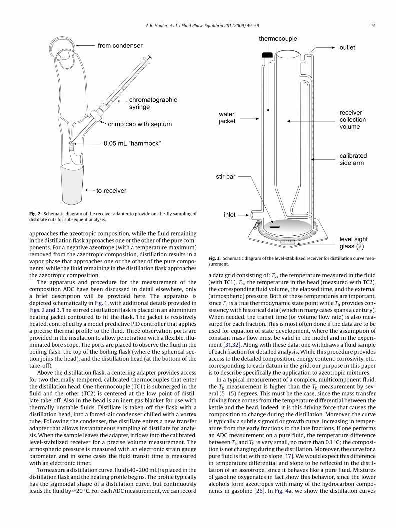
ig. 2. Schematic diagram of the receiver adapter to provide on-the-fly sampling ofistillate cuts for subsequent analysis.

pproaches the azeotropic composition, while the fluid remainingn the distillation flask approaches one or the other of the pure com-onents. For a negative azeotrope (with a temperature maximum)emoved from the azeotropic composition, distillation results in aapor phase that approaches one or the other of the pure compo-ents, while the fluid remaining in the distillation flask approacheshe azeotropic composition.

The apparatus and procedure for the measurement of theomposition ADC have been discussed in detail elsewhere, only

brief description will be provided here. The apparatus isepicted schematically in Fig. 1, with additional details provided inigs. 2 and 3. The stirred distillation flask is placed in an aluminiumeating jacket contoured to fit the flask. The jacket is resistivelyeated, controlled by a model predictive PID controller that appliesprecise thermal profile to the fluid. Three observation ports arerovided in the insulation to allow penetration with a flexible, illu-inated bore scope. The ports are placed to observe the fluid in the

oiling flask, the top of the boiling flask (where the spherical sec-ion joins the head), and the distillation head (at the bottom of theake-off).

Above the distillation flask, a centering adapter provides accessor two thermally tempered, calibrated thermocouples that enterhe distillation head. One thermocouple (TC1) is submerged in theuid and the other (TC2) is centered at the low point of distil-

ate take-off. Also in the head is an inert gas blanket for use withhermally unstable fluids. Distillate is taken off the flask with aistillation head, into a forced-air condenser chilled with a vortexube. Following the condenser, the distillate enters a new transferdapter that allows instantaneous sampling of distillate for analy-is. When the sample leaves the adapter, it flows into the calibrated,evel-stabilized receiver for a precise volume measurement. Thetmospheric pressure is measured with an electronic strain gaugearometer, and in some cases the fluid transit time is measured

ith an electronic timer.

To measure a distillation curve, fluid (40–200 mL) is placed in theistillation flask and the heating profile begins. The profile typicallyas the sigmoidal shape of a distillation curve, but continuously

eads the fluid by ≈20 ◦C. For each ADC measurement, we can record

Fig. 3. Schematic diagram of the level-stabilized receiver for distillation curve mea-surement.

a data grid consisting of: Tk, the temperature measured in the fluid(with TC1), Th, the temperature in the head (measured with TC2),the corresponding fluid volume, the elapsed time, and the external(atmospheric) pressure. Both of these temperatures are important,since Tk is a true thermodynamic state point while Th provides con-sistency with historical data (which in many cases spans a century).When needed, the transit time (or volume flow rate) is also mea-sured for each fraction. This is most often done if the data are to beused for equation of state development, where the assumption ofconstant mass flow must be valid in the model and in the experi-ment [31,32]. Along with these data, one withdraws a fluid sampleof each fraction for detailed analysis. While this procedure providesaccess to the detailed composition, energy content, corrosivity, etc.,corresponding to each datum in the grid, our purpose in this paperis to describe specifically the application to azeotropic mixtures.

In a typical measurement of a complex, multicomponent fluid,the Tk measurement is higher than the Th measurement by sev-eral (5–15) degrees. This must be the case, since the mass transferdriving force comes from the temperature differential between thekettle and the head. Indeed, it is this driving force that causes thecomposition to change during the distillation. Moreover, the curveis typically a subtle sigmoid or growth curve, increasing in temper-ature from the early fractions to the late fractions. If one performsan ADC measurement on a pure fluid, the temperature differencebetween Tk and Th is very small, no more than 0.1 ◦C; the composi-tion is not changing during the distillation. Moreover, the curve for apure fluid is flat with no slope [17]. We would expect this difference

in temperature differential and slope to be reflected in the distil-lation of an azeotrope, since it behaves like a pure fluid. Mixturesof gasoline oxygenates in fact show this behavior, since the loweralcohols form azeotropes with many of the hydrocarbon compo-nents in gasoline [26]. In Fig. 4a, we show the distillation curves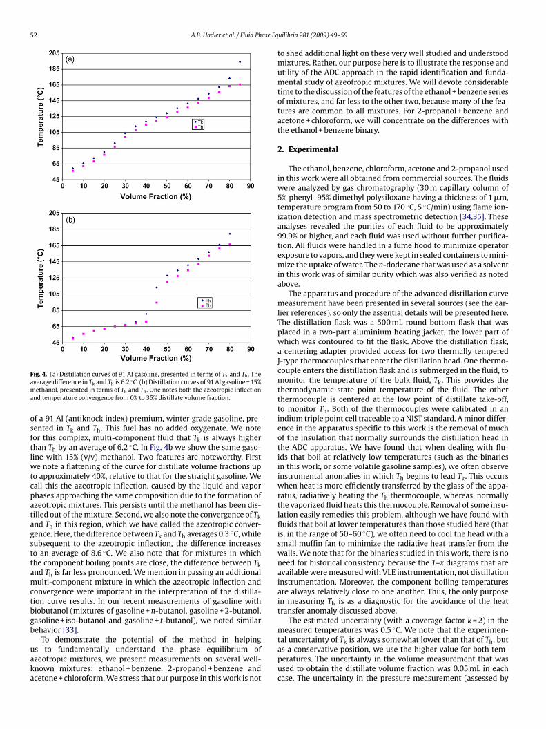

52 A.B. Hadler et al. / Fluid Phase Eq

Fama

osftlwtcpatagsttamctbgb

uaka

ig. 4. (a) Distillation curves of 91 AI gasoline, presented in terms of Tk and Th. Theverage difference in Tk and Th is 6.2 ◦C. (b) Distillation curves of 91 AI gasoline + 15%ethanol, presented in terms of Tk and Th. One notes both the azeotropic inflection

nd temperature convergence from 0% to 35% distillate volume fraction.

f a 91 AI (antiknock index) premium, winter grade gasoline, pre-ented in Tk and Th. This fuel has no added oxygenate. We noteor this complex, multi-component fluid that Tk is always higherhan Th by an average of 6.2 ◦C. In Fig. 4b we show the same gaso-ine with 15% (v/v) methanol. Two features are noteworthy. First

e note a flattening of the curve for distillate volume fractions upo approximately 40%, relative to that for the straight gasoline. Weall this the azeotropic inflection, caused by the liquid and vaporhases approaching the same composition due to the formation ofzeotropic mixtures. This persists until the methanol has been dis-illed out of the mixture. Second, we also note the convergence of Tknd Th in this region, which we have called the azeotropic conver-ence. Here, the difference between Tk and Th averages 0.3 ◦C, whileubsequent to the azeotropic inflection, the difference increaseso an average of 8.6 ◦C. We also note that for mixtures in whichhe component boiling points are close, the difference between Tknd Th is far less pronounced. We mention in passing an additionalulti-component mixture in which the azeotropic inflection and

onvergence were important in the interpretation of the distilla-ion curve results. In our recent measurements of gasoline withiobutanol (mixtures of gasoline + n-butanol, gasoline + 2-butanol,asoline + iso-butanol and gasoline + t-butanol), we noted similarehavior [33].

To demonstrate the potential of the method in helpings to fundamentally understand the phase equilibrium ofzeotropic mixtures, we present measurements on several well-nown mixtures: ethanol + benzene, 2-propanol + benzene andcetone + chloroform. We stress that our purpose in this work is not

uilibria 281 (2009) 49–59

to shed additional light on these very well studied and understoodmixtures. Rather, our purpose here is to illustrate the response andutility of the ADC approach in the rapid identification and funda-mental study of azeotropic mixtures. We will devote considerabletime to the discussion of the features of the ethanol + benzene seriesof mixtures, and far less to the other two, because many of the fea-tures are common to all mixtures. For 2-propanol + benzene andacetone + chloroform, we will concentrate on the differences withthe ethanol + benzene binary.

2. Experimental

The ethanol, benzene, chloroform, acetone and 2-propanol usedin this work were all obtained from commercial sources. The fluidswere analyzed by gas chromatography (30 m capillary column of5% phenyl–95% dimethyl polysiloxane having a thickness of 1 �m,temperature program from 50 to 170 ◦C, 5 ◦C/min) using flame ion-ization detection and mass spectrometric detection [34,35]. Theseanalyses revealed the purities of each fluid to be approximately99.9% or higher, and each fluid was used without further purifica-tion. All fluids were handled in a fume hood to minimize operatorexposure to vapors, and they were kept in sealed containers to mini-mize the uptake of water. The n-dodecane that was used as a solventin this work was of similar purity which was also verified as notedabove.

The apparatus and procedure of the advanced distillation curvemeasurement have been presented in several sources (see the ear-lier references), so only the essential details will be presented here.The distillation flask was a 500 mL round bottom flask that wasplaced in a two-part aluminium heating jacket, the lower part ofwhich was contoured to fit the flask. Above the distillation flask,a centering adapter provided access for two thermally temperedJ-type thermocouples that enter the distillation head. One thermo-couple enters the distillation flask and is submerged in the fluid, tomonitor the temperature of the bulk fluid, Tk. This provides thethermodynamic state point temperature of the fluid. The otherthermocouple is centered at the low point of distillate take-off,to monitor Th. Both of the thermocouples were calibrated in anindium triple point cell traceable to a NIST standard. A minor differ-ence in the apparatus specific to this work is the removal of muchof the insulation that normally surrounds the distillation head inthe ADC apparatus. We have found that when dealing with flu-ids that boil at relatively low temperatures (such as the binariesin this work, or some volatile gasoline samples), we often observeinstrumental anomalies in which Th begins to lead Tk. This occurswhen heat is more efficiently transferred by the glass of the appa-ratus, radiatively heating the Th thermocouple, whereas, normallythe vaporized fluid heats this thermocouple. Removal of some insu-lation easily remedies this problem, although we have found withfluids that boil at lower temperatures than those studied here (thatis, in the range of 50–60 ◦C), we often need to cool the head with asmall muffin fan to minimize the radiative heat transfer from thewalls. We note that for the binaries studied in this work, there is noneed for historical consistency because the T–x diagrams that areavailable were measured with VLE instrumentation, not distillationinstrumentation. Moreover, the component boiling temperaturesare always relatively close to one another. Thus, the only purposein measuring Th is as a diagnostic for the avoidance of the heattransfer anomaly discussed above.

The estimated uncertainty (with a coverage factor k = 2) in themeasured temperatures was 0.5 ◦C. We note that the experimen-

tal uncertainty of Tk is always somewhat lower than that of Th, butas a conservative position, we use the higher value for both tem-peratures. The uncertainty in the volume measurement that wasused to obtain the distillate volume fraction was 0.05 mL in eachcase. The uncertainty in the pressure measurement (assessed by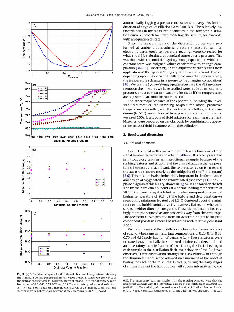

A.B. Hadler et al. / Fluid Phase Eq

Fig. 5. (a) A T–x phase diagram for the ethanol + benzene binary mixture showingthe minimum boiling positive (minimum vapor pressure) azeotrope. (b) A plot ofthe distillation curve data for binary mixtures of ethanol + benzene at benzene molefractions xb = 0.20, 0.40, 0.55, 0.70 and 0.80. The uncertainty is discussed in the text.(c) The results of the gas chromatographic analysis of distillate fractions from thestarting mixtures of ethanol + benzene at mole fractions xb = 0.20, 0.55 and

uilibria 281 (2009) 49–59 53

automatically logging a pressure measurement every 15 s for theduration of a typical distillation) was 0.001 kPa. The relatively lowuncertainties in the measured quantities in the advanced distilla-tion curve approach facilitate modeling the results, for example,with an equation of state.

Since the measurements of the distillation curves were per-formed at ambient atmospheric pressure (measured with anelectronic barometer), temperature readings were corrected forwhat should be obtained at standard atmospheric pressure. Thiswas done with the modified Sydney Young equation, in which theconstant term was assigned values consistent with Young’s com-pilation [36–38]. Uncertainty in the adjustment that results fromapplication of the Sydney Young equation can be several degrees,depending upon the slope of distillation curve (that is, how rapidlythe temperatures change in response to the changing composition)[39]. We use the Sydney Young equation because the VLE measure-ments on the mixtures we have studied were made at atmosphericpressure, and a comparison can only be made if the temperaturesare adjusted to account for our elevation.

The other major features of the apparatus, including the level-stabilized receiver, the sampling adapter, the model predictivetemperature controller, and the vortex tube chilling of the con-denser (to 5 ◦C), are unchanged from previous reports. In this work,we used 200 mL aliquots of fluid mixture for each measurement.Mixtures were prepared on a molar basis by combining the appro-priate mass of fluid in stoppered mixing cylinders.

3. Results and discussion

3.1. Ethanol + benzene

One of the most well-known minimum boiling binary azeotropeis that formed by benzene and ethanol [40–42]. It is often presentedin introductory texts as an instructional example because of thestriking features and structure of the phase diagram (the tempera-ture differences are significant, the two-phase region is large, andthe azeotrope occurs nearly at the midpoint of the T–x diagram)[5,6]. This mixture is also industrially important in the formulationand design of oxygenated and reformulated gasolines [43]. The T–xphase diagram of this binary, shown in Fig. 5a, is anchored on the leftside by the pure ethanol point (at a normal boiling temperature of78.4 ◦C), and on the right side by the pure benzene point (at a normalboiling temperature of 80.1 ◦C). The bubble and dew point curvesmeet at the minimum located at 68.2 ◦C. Centered about the mini-mum on the bubble point curve is a relatively flat region where theslopes in either direction are gentle. These slopes become increas-ingly more pronounced as one proceeds away from the azeotrope.The dew point curves proceed from the azeotropic point to the purecomponent points in a more linear fashion with relatively constantslope.

We have measured the distillation behavior for binary mixturesof ethanol + benzene with starting compositions of 0.20, 0.40, 0.55,0.70 and 0.80 mole fraction of benzene (xb). These mixtures wereprepared gravimetrically in stoppered mixing cylinders, and hadan uncertainty in mole fraction of 0.01. During the initial heating ofeach sample in the distillation flask, the behavior of the fluid was

observed. Direct observation through the flask window or throughthe illuminated bore scope allowed measurement of the onset ofboiling for each of the mixtures. Typically, during the early stagesof a measurement the first bubbles will appear intermittently, and

0.80. The uncertainty bars are smaller than the plotting symbols. Note that thepoints that coincide with the left vertical axis are at a distillate fraction of 0.00025(0.025%). (d) The enthalpy of combustion as a function of distillate fraction for theethanol + benzene mixtures presented in (c). The uncertainty is discussed in the text.

54 A.B. Hadler et al. / Fluid Phase Eq

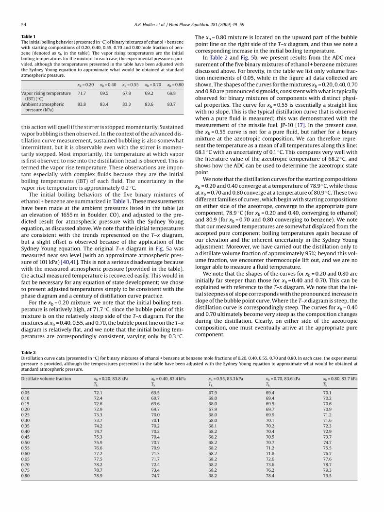
Table 1The initial boiling behavior (presented in ◦C) of binary mixtures of ethanol + benzenewith starting compositions of 0.20, 0.40, 0.55, 0.70 and 0.80 mole fraction of ben-zene (denoted as xb in the table). The vapor rising temperatures are the initialboiling temperatures for the mixture. In each case, the experimental pressure is pro-vided, although the temperatures presented in the table have been adjusted withthe Sydney Young equation to approximate what would be obtained at standardatmospheric pressure.

xb = 0.20 xb = 0.40 xb = 0.55 xb = 0.70 xb = 0.80

V

A

tvtitittbv

ehadeabSmswtftp

pmmdp

TDps

D

0000000000000000

apor rising temperature(IBT) (◦C)

71.7 69.5 67.8 69.2 69.8

mbient atmosphericpressure (kPa)

83.8 83.4 83.3 83.6 83.7

his action will quell if the stirrer is stopped momentarily. Sustainedapor bubbling is then observed. In the context of the advanced dis-illation curve measurement, sustained bubbling is also somewhatntermittent, but it is observable even with the stirrer is momen-arily stopped. Most importantly, the temperature at which vapors first observed to rise into the distillation head is observed. This isermed the vapor rise temperature. These observations are impor-ant especially with complex fluids because they are the initialoiling temperatures (IBT) of each fluid. The uncertainty in theapor rise temperature is approximately 0.2 ◦C.

The initial boiling behaviors of the five binary mixtures ofthanol + benzene are summarized in Table 1. These measurementsave been made at the ambient pressures listed in the table (atn elevation of 1655 m in Boulder, CO), and adjusted to the pre-icted result for atmospheric pressure with the Sydney Youngquation, as discussed above. We note that the initial temperaturesre consistent with the trends represented on the T–x diagram,ut a slight offset is observed because of the application of theydney Young equation. The original T–x diagram in Fig. 5a waseasured near sea level (with an approximate atmospheric pres-

ure of 101 kPa) [40,41]. This is not a serious disadvantage becauseith the measured atmospheric pressure (provided in the table),

he actual measured temperature is recovered easily. This would inact be necessary for any equation of state development; we choseo present adjusted temperatures simply to be consistent with thehase diagram and a century of distillation curve practice.

For the xb = 0.20 mixture, we note that the initial boiling tem-

erature is relatively high, at 71.7 ◦C, since the bubble point of thisixture is on the relatively steep side of the T–x diagram. For theixtures at xb = 0.40, 0.55, and 0.70, the bubble point line on the T–x

iagram is relatively flat, and we note that the initial boiling tem-eratures are correspondingly consistent, varying only by 0.3 ◦C.

able 2istillation curve data (presented in ◦C) for binary mixtures of ethanol + benzene at benzressure is provided, although the temperatures presented in the table have been adjutandard atmospheric pressure.

istillate volume fraction xb = 0.20, 83.8 kPa xb = 0.40, 83.4 kPaTk Tk

.05 72.1 69.5

.10 72.4 69.7

.15 72.6 69.6

.20 72.9 69.7

.25 73.3 70.0

.30 73.7 70.1

.35 74.2 70.2

.40 74.7 70.2

.45 75.3 70.4

.50 75.9 70.7

.55 76.6 70.9

.60 77.2 71.3

.65 77.5 71.7

.70 78.2 72.4

.75 78.7 73.4

.80 78.9 74.7

uilibria 281 (2009) 49–59

The xb = 0.80 mixture is located on the upward part of the bubblepoint line on the right side of the T–x diagram, and thus we note acorresponding increase in the initial boiling temperature.

In Table 2 and Fig. 5b, we present results from the ADC mea-surement of the five binary mixtures of ethanol + benzene mixturesdiscussed above. For brevity, in the table we list only volume frac-tion increments of 0.05, while in the figure all data collected areshown. The shapes of the curves for the mixtures xb = 0.20, 0.40, 0.70and 0.80 are pronounced sigmoids, consistent with what is typicallyobserved for binary mixtures of components with distinct physi-cal properties. The curve for xb = 0.55 is essentially a straight linewith no slope. This is the typical distillation curve that is observedwhen a pure fluid is measured; this was demonstrated with themeasurement of the missile fuel, JP-10 [17]. In the present case,the xb = 0.55 curve is not for a pure fluid, but rather for a binarymixture at the azeotropic composition. We can therefore repre-sent the temperature as a mean of all temperatures along this line:68.1 ◦C with an uncertainty of 0.1 ◦C. This compares very well withthe literature value of the azeotropic temperature of 68.2 ◦C, andshows how the ADC can be used to determine the azeotropic statepoint.

We note that the distillation curves for the starting compositionsxb = 0.20 and 0.40 converge at a temperature of 78.9 ◦C, while thoseat xb = 0.70 and 0.80 converge at a temperature of 80.9 ◦C. These twodifferent families of curves, which begin with starting compositionson either side of the azeotrope, converge to the appropriate purecomponent, 78.9 ◦C (for xb = 0.20 and 0.40, converging to ethanol)and 80.9 (for xb = 0.70 and 0.80 converging to benzene). We notethat our measured temperatures are somewhat displaced from theaccepted pure component boiling temperatures again because ofour elevation and the inherent uncertainty in the Sydney Youngadjustment. Moreover, we have carried out the distillation only toa distillate volume fraction of approximately 95%; beyond this vol-ume fraction, we encounter thermocouple lift out, and we are nolonger able to measure a fluid temperature.

We note that the shapes of the curves for xb = 0.20 and 0.80 areinitially far steeper than those for xb = 0.40 and 0.70. This can beexplained with reference to the T–x diagram. We note that the ini-tial steepness of slope corresponds with the pronounced increase inslope of the bubble point curve. Where the T–x diagram is steep, the

distillation curve is correspondingly steep. The curves for xb = 0.40and 0.70 ultimately become very steep as the composition changesduring the distillation. Clearly, on either side of the azeotropiccomposition, one must eventually arrive at the appropriate purecomponent.

ene mole fractions of 0.20, 0.40, 0.55, 0.70 and 0.80. In each case, the experimentalsted with the Sydney Young equation to approximate what would be obtained at

xb = 0.55, 83.3 kPa xb = 0.70, 83.6 kPa xb = 0.80, 83.7 kPaTk Tk Tk

67.9 69.4 70.168.0 69.4 70.268.0 69.5 70.667.9 69.7 70.968.0 69.9 71.268.0 70.1 71.668.1 70.2 72.368.2 70.4 72.968.2 70.5 73.768.2 70.7 74.768.2 71.2 75.568.2 71.8 76.768.2 72.6 77.668.2 73.6 78.768.2 76.2 79.368.2 78.4 79.5

ase Equilibria 281 (2009) 49–59 55

dsttt0mscdaflpat(m

atdTtasca

tTpltbofktdxetaldbptd18sido

tetf[ideo

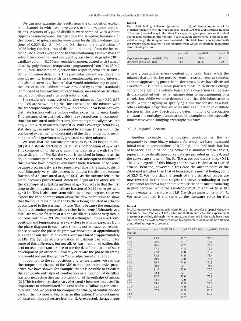
Table 3The initial boiling behavior (presented in ◦C) of binary mixtures of 2-propanol + benzene with starting compositions of 0.20, 0.65 and 0.80 mole fractionof benzene (denoted as xb in the table). The vapor rising temperatures are the initialboiling temperatures for the mixture. In each case, the experimental pressure is pro-vided, although the temperatures presented in the table have been adjusted withthe Sydney Young equation to approximate what would be obtained at standardatmospheric pressure.

now reversed in the later stages; the curve terminating at pure2-propanol reaches a higher temperature than the one terminatingin pure benzene, while the azeotropic mixture at xb = 0.61 is flatat an average temperature of 71.9 ◦C with an uncertainty of 0.1 ◦C.We note that this is the same as the literature value for this

Table 4Distillation curve data (presented in ◦C) for binary mixtures of 2-propanol + benzeneat benzene mole fractions of 0.20, 0.65, and 0.80. In each case, the experimentalpressure is provided, although the temperatures presented in the table have beenadjusted with the Sydney Young equation to approximate what would be obtainedat standard atmospheric pressure.

Distillate volumefraction

xb = 0.20, 83.0 kPa xb = 0.65, 83.6 kPa xb = 0.80, 83.2 kPa

0.05 75.9 71.7 72.50.10 76.1 71.7 72.60.15 76.6 71.7 72.80.20 77.1 71.8 72.90.25 77.8 71.8 73.20.30 78.3 71.9 73.40.35 79.0 72.0 73.80.40 79.7 71.9 74.30.45 80.8 72.1 74.80.50 81.7 72.0 75.70.55 82.4 72.1 76.70.60 82.9 72.0 77.90.65 83.1 72.0 79.0

A.B. Hadler et al. / Fluid Ph

We can now examine the results from the composition explicitata channel, in which we have access to the dew point compo-itions. Aliquots of 7 �L of distillate were sampled with a bluntipped chromatographic syringe from the sampling hammock ofhe receiver adapter. Samples were taken for distillate volume frac-ions of 0.025, 0.2, 0.4, 0.6, and 0.8, the sample at a fraction of.025 being the first drop of distillate to emerge from the instru-ent. The aliquots were added to a vial containing a known mass of

olvent (n-dodecane), and analyzed by gas chromatography (30 mapillary column, 0.250 mm outside diameter, coated with 1 �m ofimethyl polysiloxane, temperature programmed from 90 to 250 ◦Ct 8 ◦C/min, autosampler injection into a split injector set at 100:1,ame ionization detection). This particular solvent was chosen torovide no interference with the chromatographic peaks of interest,nd also to serve as a “keeper” that would minimize any evapora-ive loss of solute. Calibration was provided by external standardscomprised of four mixtures of each binary) measured on the chro-

atograph before and after each solution cut.The results of the analysis of starting mixtures of xb = 0.20, 0.55

nd 0.80 are shown in Fig. 5c. One can see that the mixture withhe azeotropic composition of xb = 0.55 shows linear behavior withistillate fraction, with zero slope within experimental uncertainty.his mixture, when distilled, yields the expected constant composi-ion. Our measured mole fractions (chromatographically measuredt xb = 0.57 with an uncertainty of 0.02, with a coverage factor k = 2),tatistically, can only be represented by a mean. This is within theombined experimental uncertainty of the chromatographic resultnd that of the gravimetrically prepared starting mixture.

We note that the mixture prepared as xb = 0.20 begins to dis-ill (at a distillate fraction of 0.025) at a composition of xb = 0.47.his composition of the dew point line is consistent with the T–xhase diagram of Fig. 5a; the vapor is enriched in benzene as the

iquid becomes pure ethanol. We see that subsequent fractions ofhis mixture have progressively lower mole fractions of benzene,ecause progressively less benzene is available in the liquid to distillut. Ultimately, very little benzene is found at the distillate volumeraction of 0.8 (measured at xb = 0.004), as the mixture left in theettle becomes pure ethanol. When we begin on the other side ofhe azeotrope, at a starting mixture of xb = 0.80, we see that the firstrop to distill (again at a distillate fraction of 0.025) emerges withb = 0.64. This is also consistent with the phase diagram, since wexpect the vapor composition along the dew point curve to showhat the liquid remaining in the kettle is being depleted in ethanols compared to the starting mixture. This is because the remainingiquid is becoming progressively richer in benzene. Ultimately, at aistillate volume fraction of 0.8, the distillate is indeed very rich inenzene, with xb = 0.99. We note that although our measured com-ositions and temperatures are very close to what is expected fromhe phase diagram in each case, there is not an exact correspon-ence because the phase diagram was measured at approximately01 kPa and our distillation curves were measured at approximately3 kPa. The Sydney Young equation adjustment can account forome of this difference, but not all. As was mentioned earlier, thiss of no real importance, since to use the data for equation of stateevelopment (in order to ultimately calculate the phase diagram),ne would not use the Sydney Young adjustment at all [39].

In addition to the compositions and temperatures, we can usehe composition channel of the ADC to obtain other intensive prop-rties. We have shown, for example, that it is possible to calculatehe composite enthalpy of combustion as a function of distillateraction, neglecting the small contribution of the enthalpy of mixing

21]. This is relevant to the binary of ethanol + benzene because of itsmportance to reformulated fuels and biofuels. Following the proce-ure outlined, we present the composite enthalpy of combustion forach of the mixtures in Fig. 5d as an illustration. The uncertaintiesf these enthalpy values are less than 3. As expected, the azeotrope

xb = 0.20 xb = 0.61 xb = 0.80

Vapor rise temperature (IBT) (◦C) 75.3 71.6 72.1Observed pressure (kPa) 83.0 83.6 83.2

is nearly constant in energy content on a molar basis, while themixture that approaches pure benzene increases in energy content,and that approaching pure ethanol decreases. As we have discussedelsewhere, it is often a more practical measure to discuss energycontent of a fuel on a volume basis, and a conversion can be eas-ily accomplished with either mixture density measurements or acorrelation. While we have demonstrated that this information isuseful when designing or specifying a mixture for use as a fuel,other enthalpic properties are accessible as a function of distillatefraction in this way. Spectroscopic determinations of associationconstant and enthalpy of association, for example, can be especiallyinformative when studying azeotropic mixtures.

3.2. 2-Propanol + benzene

Another example of a positive azeotrope is the 2-propanol + benzene binary mixture, for which we have measuredinitial mixture compositions of 0.20, 0.61, and 0.80 mole fractionof benzene. The initial boiling behavior is summarized in Table 3,representative distillation curve data are provided in Table 4, andthe curves are shown in Fig. 6a. The azeotrope occurs at xb = 0.61.The T–x diagram of this binary (not shown) is similar to that ofethanol benzene, however in this case the anchor point of the2-butanol is higher than that of benzene, at a normal boiling pointof 82.5 ◦C. We note that the trends of the distillation curves are

0.70 83.1 71.9 79.60.75 83.1 71.9 80.10.80 82.9 71.9 80.10.85 71.8 80.00.90 71.7

56 A.B. Hadler et al. / Fluid Phase Equilibria 281 (2009) 49–59

Fig. 6. (a) A plot of the distillation curve data for binary mixtures of 2-propanol + benzene at benzene mole fractions of 0.20, 0.65 and 0.80. The uncertaintyis discussed in the text. (b) The results of the gas chromatographic analysis of dis-tap(

atc

sansuocawtgt

aaaa

3

am

Fig. 7. (a) A T–x diagram for the mixture acetone + chloroform, showing the max-imum boiling negative (minimum vapor pressure) azeotrope. (b) A plot of thedistillation curve data for binary mixtures of acetone + chloroform at chloroformmole fractions of 0.05, 0.10, 0.20, 0.50, 0.65, 0.70, and 0.85. The uncertainty is dis-cussed in the text. (c) The results of the gas chromatographic analysis of distillate

illate fractions from the starting mixtures of 2-propanol + benzene at xb = 0.20, 0.61nd 0.80. The uncertainty bars are smaller than the plotting symbols. Note that theoints that coincide with the left vertical axis are at a distillate fraction of 0.000250.025%).

zeotropic state point [40,41,44]. The curve for xb = 0.80 convergeso a temperature of 80.1 ◦C (pure benzene), while the xb = 0.20urve converges to 83.0 ◦C (pure 2-propanol).

The results from the composition explicit data channel (mea-ured similarly to that of ethanol + benzene), are shown in Fig. 6b,nd we note a consistency with the distillation curves. First, weote that the measured composition of the azeotrope line is con-tant and can be best represented by a mean of xb = 0.62 with anncertainty of 0.01, which is within the experimental uncertaintyf the literature value of the composition (xb = 0.61). The measuredompositions of the 0.025 distillate volume fractions of the xb = 0.20nd 0.80 are not at the starting mole fractions of the mixtures, bute note that they are immediately shifted to the compositions of

he dew point line. This is the behavior expected from the T–x dia-ram. Thereafter, there is a progression to the pure fluid, as withhe ethanol + benzene binary.

We note that the behavior discussed above is easily distinguish-ble from mixtures that are zeotropic. For zeotropic mixtures, forny starting composition, the distillation temperature will gradu-lly approach that of the less volatile component [14]. The gradualpproach is indicative of small deviations from Raoult’s law.

.3. Acetone + chloroform

Negative azeotropes are far less common than positivezeotropes, and are therefore more difficult to study. It is simplyore difficult to find a mixture that is amenable to a particular

fractions from the starting mixtures of acetone + chloroform at xc = 0.05, 0.10, 0.20,0.50, 0.65, 0.70, and 0.85. The uncertainty bars are smaller than the plotting symbols.Note that the points that coincide with the left vertical axis are at a distillate fractionof 0.00025 (0.025%).

metrology. A well-known example of a negative azeotropic binarymixture is the acetone + chloroform mixture, the T–x diagram forwhich is presented in Fig. 7a. The diagram is anchored on the leftside by the pure acetone point (at a normal boiling temperature

A.B. Hadler et al. / Fluid Phase Equilibria 281 (2009) 49–59 57

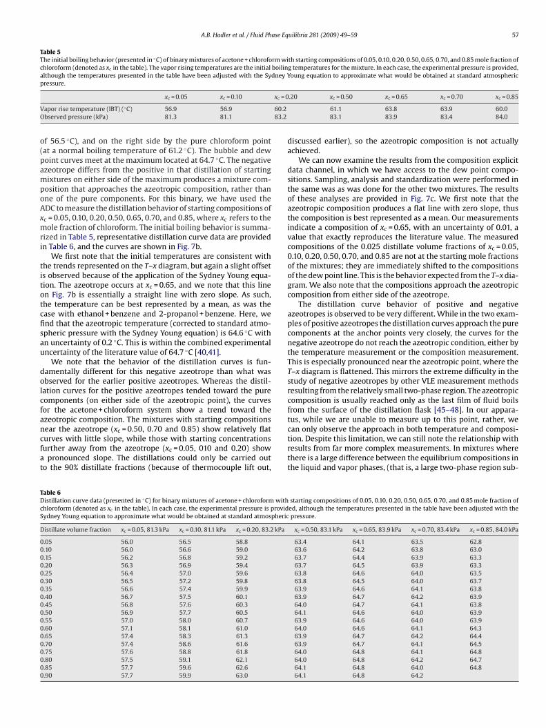
Table 5The initial boiling behavior (presented in ◦C) of binary mixtures of acetone + chloroform with starting compositions of 0.05, 0.10, 0.20, 0.50, 0.65, 0.70, and 0.85 mole fraction ofchloroform (denoted as xc in the table). The vapor rising temperatures are the initial boiling temperatures for the mixture. In each case, the experimental pressure is provided,although the temperatures presented in the table have been adjusted with the Sydney Young equation to approximate what would be obtained at standard atmosphericpressure.

xc = 0

V 60.2O 83.2

o(pampoAxmri

titotcfisau

dolcfancfat

TDcS

D

000000000000000000

xc = 0.05 xc = 0.10

apor rise temperature (IBT) (◦C) 56.9 56.9bserved pressure (kPa) 81.3 81.1

f 56.5 ◦C), and on the right side by the pure chloroform pointat a normal boiling temperature of 61.2 ◦C). The bubble and dewoint curves meet at the maximum located at 64.7 ◦C. The negativezeotrope differs from the positive in that distillation of startingixtures on either side of the maximum produces a mixture com-

osition that approaches the azeotropic composition, rather thanne of the pure components. For this binary, we have used theDC to measure the distillation behavior of starting compositions ofc = 0.05, 0.10, 0.20, 0.50, 0.65, 0.70, and 0.85, where xc refers to theole fraction of chloroform. The initial boiling behavior is summa-

ized in Table 5, representative distillation curve data are providedn Table 6, and the curves are shown in Fig. 7b.

We first note that the initial temperatures are consistent withhe trends represented on the T–x diagram, but again a slight offsets observed because of the application of the Sydney Young equa-ion. The azeotrope occurs at xc = 0.65, and we note that this linen Fig. 7b is essentially a straight line with zero slope. As such,he temperature can be best represented by a mean, as was thease with ethanol + benzene and 2-propanol + benzene. Here, wend that the azeotropic temperature (corrected to standard atmo-pheric pressure with the Sydney Young equation) is 64.6 ◦C withn uncertainty of 0.2 ◦C. This is within the combined experimentalncertainty of the literature value of 64.7 ◦C [40,41].

We note that the behavior of the distillation curves is fun-amentally different for this negative azeotrope than what wasbserved for the earlier positive azeotropes. Whereas the distil-ation curves for the positive azeotropes tended toward the pureomponents (on either side of the azeotropic point), the curvesor the acetone + chloroform system show a trend toward thezeotropic composition. The mixtures with starting compositions

ear the azeotrope (xc = 0.50, 0.70 and 0.85) show relatively flaturves with little slope, while those with starting concentrationsurther away from the azeotrope (xc = 0.05, 010 and 0.20) show

pronounced slope. The distillations could only be carried outo the 90% distillate fractions (because of thermocouple lift out,

able 6istillation curve data (presented in ◦C) for binary mixtures of acetone + chloroform withhloroform (denoted as xc in the table). In each case, the experimental pressure is providydney Young equation to approximate what would be obtained at standard atmospheric

istillate volume fraction xc = 0.05, 81.3 kPa xc = 0.10, 81.1 kPa xc = 0.20, 83.2 kPa

.05 56.0 56.5 58.8

.10 56.0 56.6 59.0

.15 56.2 56.8 59.2

.20 56.3 56.9 59.4

.25 56.4 57.0 59.6

.30 56.5 57.2 59.8

.35 56.6 57.4 59.9

.40 56.7 57.5 60.1

.45 56.8 57.6 60.3

.50 56.9 57.7 60.5

.55 57.0 58.0 60.7

.60 57.1 58.1 61.0

.65 57.4 58.3 61.3

.70 57.4 58.6 61.6

.75 57.6 58.8 61.8

.80 57.5 59.1 62.1

.85 57.7 59.6 62.6

.90 57.7 59.9 63.0

.20 xc = 0.50 xc = 0.65 xc = 0.70 xc = 0.85

61.1 63.8 63.9 60.083.1 83.9 83.4 84.0

discussed earlier), so the azeotropic composition is not actuallyachieved.

We can now examine the results from the composition explicitdata channel, in which we have access to the dew point compo-sitions. Sampling, analysis and standardization were performed inthe same was as was done for the other two mixtures. The resultsof these analyses are provided in Fig. 7c. We first note that theazeotropic composition produces a flat line with zero slope, thusthe composition is best represented as a mean. Our measurementsindicate a composition of xc = 0.65, with an uncertainty of 0.01, avalue that exactly reproduces the literature value. The measuredcompositions of the 0.025 distillate volume fractions of xc = 0.05,0.10, 0.20, 0.50, 0.70, and 0.85 are not at the starting mole fractionsof the mixtures; they are immediately shifted to the compositionsof the dew point line. This is the behavior expected from the T–x dia-gram. We also note that the compositions approach the azeotropiccomposition from either side of the azeotrope.

The distillation curve behavior of positive and negativeazeotropes is observed to be very different. While in the two exam-ples of positive azeotropes the distillation curves approach the purecomponents at the anchor points very closely, the curves for thenegative azeotrope do not reach the azeotropic condition, either bythe temperature measurement or the composition measurement.This is especially pronounced near the azeotropic point, where theT–x diagram is flattened. This mirrors the extreme difficulty in thestudy of negative azeotropes by other VLE measurement methodsresulting from the relatively small two-phase region. The azeotropiccomposition is usually reached only as the last film of fluid boilsfrom the surface of the distillation flask [45–48]. In our appara-tus, while we are unable to measure up to this point, rather, we

can only observe the approach in both temperature and composi-tion. Despite this limitation, we can still note the relationship withresults from far more complex measurements. In mixtures wherethere is a large difference between the equilibrium compositions inthe liquid and vapor phases, (that is, a large two-phase region sub-

starting compositions of 0.05, 0.10, 0.20, 0.50, 0.65, 0.70, and 0.85 mole fraction ofed, although the temperatures presented in the table have been adjusted with thepressure.

xc = 0.50, 83.1 kPa xc = 0.65, 83.9 kPa xc = 0.70, 83.4 kPa xc = 0.85, 84.0 kPa

63.4 64.1 63.5 62.863.6 64.2 63.8 63.063.7 64.4 63.9 63.363.7 64.5 63.9 63.363.8 64.6 64.0 63.563.8 64.5 64.0 63.763.9 64.6 64.1 63.863.9 64.7 64.2 63.964.0 64.7 64.1 63.864.1 64.6 64.0 63.963.9 64.6 64.0 63.964.0 64.6 64.1 64.363.9 64.7 64.2 64.463.9 64.7 64.1 64.564.0 64.8 64.1 64.864.0 64.8 64.2 64.764.1 64.8 64.0 64.864.1 64.8 64.2

5 ase Eq

tFaaatbtb�aFdtstoa

4

btsopiiimddAccefdieldb

A

mwC

R

[

[

[

[

[

[

[

[

[

[

[

[

[

[

[

[

8 A.B. Hadler et al. / Fluid Ph

ended by the bubble and dew point lines shown, for example inig. 5a), the composition in the boiler will change more rapidly andpproach the anchor point component quickly. For mixtures withsmall difference between equilibrium compositions in the liquidnd vapor phases (that is, a small two-phase region subtended byhe bubble and dew point lines shown, for example in Fig. 7a), theoiler composition will change slowly. For these phase diagrams,he largest changes in the compositions will occur when (Vo − �V)ecomes small, where Vo is the initial volume in the kettle, andV is the change in volume in the kettle [47]. The ADC method

llows rapid identification of the presence of negative azeotropy.or compositions starting near the more volatile component, theistillation temperature slowly increases to temperatures abovehe boiling point of the more volatile component; for compositionstarting near the less volatile component, the distillation tempera-ure slowly increases to temperatures above the initial boiling pointf mixture. These are indications that the mixture has a negativezeotrope.

. Conclusions

In this paper, we have discussed how the ADC metrology cane used to detect and identify azeotropic fluid behavior (withhe azeotropic inflection and convergence). We have also demon-trated that the method can be used to study the fundamentalsf azeotropic phase equilibrium in a rapid and economical way,roviding bubble point temperature and dew point composition

nformation. The shapes of the distillation curves provide insightnto the shapes of the corresponding T–x diagrams, as well as anmmediate indication as to which side of the azeotrope a given

ixture originates. Moreover, this shape gives an indication of theeviations from Raoult’s law, with steeper curves indicating largereviations. Both the temperature and composition channels of theDC provide a rapid avenue to the identification of the azeotropicomposition, as well as the pure component anchor points. Theomposition channel provides access to many other intensive prop-rties in addition to the phase equilibrium information. Theseeatures of the ADC method provide the basis for equation of stateevelopment, as we have demonstrated elsewhere. We note that

n this paper we have only studied azeotropic behavior near ambi-nt pressure. Clearly, azeotropic behavior occurs at both higher andower pressures. Modifications to the existing apparatus are beingesigned and implemented at this time to allow measurements atoth higher and lower pressures.

cknowledgments

This work was performed while ABH was supported by Sum-er Undergraduate Research Fellowship (SURF) award at NIST, andhile LSO held a National Academy of Science/National Researchouncil Postdoctoral Associateship Award at NIST.

eferences

[1] H.Z. Kister, Distillation Operation, McGraw-Hill, New York, 1988.[2] H.Z. Kister, Distillation Design, McGraw-Hill, New York, 1991.[3] W. Malesinski, Azeotropy and Other Theoretical Problems of Vapor-liquid Equi-

librium, Interscience, a Division of John Wiley and Sons, London, 1965.[4] W. Swietoslawski, in: K. Ridgeway (Ed.), Azeotropy and Polyazeotropy, Macmil-

lan Company, New York, 1963.[5] G.M. Barrow, Physical Chemistry, McGraw-Hill College, New York, 1996.[6] J.P. Bromberg, Physical Chemistry, Allyn and Bacon, Boston, 1984.

[7] T. Hiaki, M. Nanao, Vapor-liquid equilibria for bis (2,2,2-trifluoroethyl)ether

with several organic compounds containing oxygen, Fluid Phase Equilib. 174(1–2) (2000) 81–91.

[8] T. Hiaki, et al., Vapor-liquid equilibria for 1,1,2, 2-tetrafluoroethyl, 2,2,2-trifluoroethyl ether with several organic compounds containing oxygen, FluidPhase Equilib 182 (1–2) (2001) 189–198.

[

[

uilibria 281 (2009) 49–59

[9] T. Hiaki, et al., Vapor-liquid equilibria for 1,1,2,3,3,3-hexafluoropropyl, 2,2,2-trifluoroethyl ether with several organic solvents, Fluid Phase Equilib 194(2002) 969–979.

[10] S. Loras, et al., Phase equilibria for 1,1,1,2,3,4,4,5,5,5-decafluoropentane +2-methylfuran, 2-methylfuran plus oxolane, and 1,1,1,2,3,4,4,5,5,5-decafluoropentane + 2-methylfuran plus oxolane at 35 kPa, J. Chem. Eng.Data 47 (5) (2002) 1256–1262.

[11] A. Mejia, H. Segura, M. Cartes, Vapor-liquid equilibrium, densities, and interfa-cial tensions for the system benzene plus propan-1-ol, Phys. Chem. Liq. 46 (2)(2008) 185–200.

[12] A. Mejia, et al., Vapor-liquid equilibrium, densities, and interfacial tensions forthe system ethyl 1, 1-dimethylethyl ether (ETBE) plus propan-1-ol, Fluid PhaseEquilib. 255 (2) (2007) 121–130.

[13] R.M. Villamanan, et al., Vapor-liquid equilibrium of binary and ternary mixturescontaining isopropyl ether, 2-butanol, and benzene at T = 313.15 K, J. Chem. Eng.Data 51 (1) (2006) 148–152.

[14] T.J. Bruno, Improvements in the measurement of distillation curves. Part 1. Acomposition-explicit approach, Ind. Eng. Chem. Res. 45 (2006) 4371–4380.

[15] T.J. Bruno, B.L. Smith, Improvements in the measurement of distillation curves-part 2: application to aerospace/aviation fuels RP-1 and S-8, Ind. Eng. Chem.Res. 45 (2006) 4381–4388.

[16] T.J. Bruno, Method and apparatus for precision in-line sampling of distillate,Sep. Sci. Technol. 41 (2) (2006) 309–314.

[17] T.J. Bruno, M.L. Huber, A. Laesecke, E.W. Lemmon, R.A. Perkins, Thermochemi-cal and thermophysical properties of JP-10, NIST-IR 6640, National Institute ofStandards and Technology (U.S.A.), 2006.

[18] T.J. Bruno, Thermodynamic, transport and chemical properties of “reference”JP-8. Book of Abstracts, Army Research Office and Air Force Office of ScientificResearch, 2006 Contractor’s meeting in Chemical Propulsion, 2006, pp. 15–18.

[19] T.J. Bruno, The properties of S-8, Final Report for MIPR F4FBEY6237G001, AirForce Research Laboratory, 2006.

20] T.J. Bruno, A. Laesecke, S.L. Outcalt, H.-D. Seelig, B.L. Smith, Properties of a 50/50mixture of Jet-A + S-8, NIST-IR-6647, 2007.

[21] T.J. Bruno, B.L. Smith, Enthalpy of combustion of fuels as a function of distil-late cut: application of an advanced distillation curve method, Energy Fuels 20(2006) 2109–2116.

22] L.S. Ott, T.J. Bruno, Corrosivity of fluids as a function of distillate cut: appli-cation of an advanced distillation curve method, Energy Fuels 21 (2007)2778–2784.

23] L.S. Ott, B.L. Smith, T.J. Bruno, Composition-explicit distillation curves of mix-tures of diesel fuel with biomass-derived glycol ester oxygenates: a fueldesign tool for decreased particulate emissions, Energy Fuels 22 (2008)2518–2526.

24] B.L. Smith, L.S. Ott, T.J. Bruno, Composition-explicit distillation curves of dieselfuel with glycol ether and glycol ester oxygenates: a design tool for decreasedparticulate emissions, Environ. Sci. Technol. 42 (20) (2008) 7682–7689.

25] B.L. Smith, T.J. Bruno, Advanced distillation curve measurement with a modelpredictive temperature controller, Int. J. Thermophys. 27 (2006) 1419–1434.

26] B.L. Smith, T.J. Bruno, Improvements in the measurement of distillation curves.Part 3. Application to gasoline and gasoline + methanol mixtures, Ind. Eng.Chem. Res. 46 (2006) 297–309.

27] B.L. Smith, T.J. Bruno, Improvements in the measurement of distillation curves.Part 4. Application to the aviation turbine fuel Jet-A, Ind. Eng. Chem. Res. 46(2006) 310–320.

28] B.L. Smith, T.J. Bruno, Application of a composition-explicit distillation curvemetrology to mixtures of Jet-A + synthetic Fischer-Tropsch S-8, J. Propul. Power24 (3) (2008) 619–623.

29] B.L. Smith, L.S. Ott, T.J. Bruno, Composition-explicit distillation curves of com-mercial biodiesel fuels: comparison of petroleum derived fuel with B20 andB100, Ind. Eng. Chem. Res. 47 (16) (2008) 5832–5840.

30] E.W. Lemmon, M.O. McLinden, M.L. Huber, REFPROP, reference fluid thermo-dynamic and transport properties NIST Standard Reference Database 23, 2005,National Institute of Standards and Technology, Gaithersburg, MD, 2005.

[31] M.L. Huber, B.L. Smith, L.S. Ott, T.J. Bruno, Surrogate mixture model for thethermophysical properties of synthetic aviation fuel S-8: explicit application ofthe advanced distillation curve, Energy Fuels 22 (2008) 1104–1114.

32] M.L. Huber, E.W. Lemmon, V. Diky, B.L. Smith, T.J. Bruno, Chemically authenticsurrogate mixture model for the thermophysical properties of a coal-derived-liquid fuel, Energy Fuels 22 (2008) 3249–3257.

33] T.J. Bruno, A. Wolk, A. Naydich, Composition-explicit distillation curves for mix-tures of gasoline with four-carbon alcohols (butanols), Energy Fuels 23 (4)(2009) 2295–2306.

34] T.J. Bruno, P.D.N. Svoronos, CRC Handbook of Basic Tables for Chemical Analysis,2nd ed., Taylor and Francis CRC Press, Boca Raton, 2004.

35] T.J. Bruno, P.D.N. Svoronos, CRC Handbook of Fundamental Spectroscopic Cor-relation Charts, Taylor and Francis CRC Press, Boca Raton, 2005.

36] S. Young, Correction of boiling points of liquids from observed to normal pres-sures, Proc. Chem. Soc. 81 (1902) 777.

[37] S. Young, Fractional Distillation, Macmillan and Co., Ltd., London, 1903.38] S. Young, Distillation Principles and Processes, Macmillan and Co., Ltd., London,

1922.39] L.S. Ott, B.L. Smith, T.J. Bruno, Experimental test of the Sydney Young equation

for the presentation of distillation curves, J. Chem. Thermodynam. 40 (2008)1352–1357.

40] J. Gmehling, J. Menke, J. Krafczk, K. Fischer, Azeotropic Data, Parts 1, 2 and 3,2nd extended ed., Wiley VCH, Weinheim, 2004.

ase Eq

[

[

[

[

[[

A.B. Hadler et al. / Fluid Ph

41] E.W. Eashburn (Ed.), International Critical Tables (of Numerical Data, PhysicsChemistry and Technology), vol. III, McGraw-Hill Book Co., 1928.

42] R. Fritzweiler, Z. Dietrich, Der Azeotropismus und seine anwendung fur neusesverfahren sur entwasserung des aethylalkohols, Angew. Chem. 46 (1933)

241.

43] A literature review based assessment on the impacts of a 10% and 20% ethanolgasoline fuel blend on non-automotive engines. 2002, Report to EnvironmentAustralia, Orbital Engine Company.

44] J.M. Rhodes, T.A. Griffin, M.J. Lazzaroni, V.R. Bhenthanabotla, S.W. Campbell,Total pressure measurements for benzene with 1-propanol, 2-propanol, 1-

[

[

uilibria 281 (2009) 49–59 59

pentanol, 3-pentanol, and 2-methyl-2-butanol at 313.15 K, Fluid Phase Equilib.179 (2001) 217–229.

45] C.D. Holcomb, National Institute of Standards and Technology, retired. 2008.46] J.R. Noles, J.A. Zollweg, Isothermal vapor liquid equilibrium for dimethyl

ether + sulfur dioxide, Fluid Phase Equilib. 66 (3) (1991) 275–289.47] J.R. Noles, Vapor liquid equilibria of solvating binary mixtures, Department of

Chemical Engineering, Cornell University, Ithica, 1991, p. 273.48] J.R. Noles, J.A. Zollweg, Vapor-liquid equilibrium for chlorodifluo-

romethane + dimethyl ether from 283 to 395 K at pressures to 5.0 MPa, J.Chem. Eng. Data 37 (3) (1992) 306–310.