Study of a Simplified Approach in Utilizing Information from Permanent Reference ... · 2016-12-15 · Utilizing Information from Permanent Reference Station Arrays H.-J. Euler,

##### Version of Monday, September 03, 2001, 13:28 #####

Study of a Simplified Approach inUtilizing Information from

Permanent Reference Station Arrays

H.-J. Euler, C.R. Keenan, B.E. Zebhauser, Leica Geosystems AG, Switzerland

G. Wübbena, Geo++ GmbH, Germany

ABSTRACT

Permanent reference station networks are used all over theworld for surveying type applications requiring centimeteraccuracy generally reducing the worth of traditional singlebaseline methods. The well known advantages providedby reference station array information include improvedmodeling of the remaining tropospheric, ionospheric andorbit biases. Methods and concepts show the improve-ments in performance and reliability in some kind ofclosed system approaches. Standardisation discussionsunderway within RTCM target the interoperability be-tween the reference station systems and roving receiversfrom various manufacturers. One obstacle in the discus-sion, and therefore in later interoperability issues, is thecreation and proper description of the models used forderiving the biases noted above. This difficulty has to bemitigated and will vanish with time, but thisinteroperability is needed urgently. This paper details adifferent approach to utilise and distribute the informationfrom permanent reference station arrays in RTCM-formatcompact messages. The separation of different calculationtasks affords an easy and efficient standard for the transferand distribution of network information. The proposedmethod may solve the current dilemma for interoperabilitystandards.

INTRODUCTION / MOTIVATION

Real-time messages for proper interoperability betweendifferent manufacturer equipment have been issued by theRTCM Sub-Committee 104 (RTCM, 2001). All informa-tion for precise positioning using baseline approaches canbe transmitted using message types 18-21.

Because the use of single reference stations has somedisadvantages in that the accuracy and reliability of inte-ger ambiguity resolution deteriorates a few tens of kilo-meters from the reference station, networks of reference

stations are being developed to mitigate the distance-dependency of RTK solutions. With such networks, aprovider can generate measurement corrections for receiv-ers operating in the area, that is covered by the networkand he can supply this information to the user in somestandard format. As the current kinematic and high-accuracy message types do not support the use of datafrom multiple reference stations, new standards musttherefore be considered to facilitate the valuable informa-tion afforded by networks of reference stations.

The standardisation of network information and process-ing models is also necessary to reduce the sizes of thenetwork RTK corrections, as well as the transmission ofsatellite-independent error information. A simplified ap-proach of transmitting data from reference station net-works to roving users is now presented in this paper in theform of a new message standard capable of supportingreference network operations. Its use should help over-come some of the problems encountered in current net-work RTK concepts.

EXISTING CONCEPTS: FKP AND VRS

At present, there are at least two approaches availablecommercially, that provide network-based solution infor-mation to roving users. The first is based upon the trans-mission of network coefficients (also known as area cor-rection parameters or FKP, the German acronym), whilstthe second is based on the transmission of “virtual refer-ence stations” (VRS) generated from the reference stationmeasurements. A short description of these concepts fol-lows.

In the first concept, computing facilities calculate forevery satellite coefficients (FKP) covering ionospheric,tropospheric and orbit effects covering a specific networkarea at specific time intervals (at least every 10 s). Themeasurement corrections, reduced by the station-satellite

A condensed version of this draft will be presented atION GPS 2001, Salt Lake City, and published thereby.

slope distances of the reference stations, are then trans-mitted via RTCM messages Type 20/21 as well as theFKPs for interpolation via a customized RTCM Type 59message.

In the VRS concept, the rovers also receive network in-formation but additionally transmit, via NMEA messages,their approximate positions to a central computing facility.This facility calculates the station-satellite slope distancesfor these approximate positions and then, from the refer-ence station observations, interpolates the correctionscorresponding to a virtual reference station near the rover.These virtual measurements are unique to each rover andtransmitted to them via RTCM messages of Type 20/21 or18/19.

Problems of FKP and VRSBoth approaches have their respective advantages as de-tailed in WÜBBENA and WILLGALIS (2001), and LARGE etal. (2001). Of more interest are their disadvantages andhow these may affect general surveying tasks within net-works. The providers decision on complexity of themathematical correction model, the rover cannot influ-ence, is a general problem. The need to select the correct(optimal) FKPs for a rover so it can interpolate its meas-urement corrections, or VRS’ dependence on complextwo-way communications over medium-sized networkswhilst restricting user numbers are such two concept-dependent examples of problems.

Both approaches are currently using the RTCM Type 59proprietary information message. The proprietary infor-mation content has been partly distributed, but it is neitherstandardised nor released by a manufacturer independentorganisation like RTCM. However both concepts are notfully compatible with the RTCM standard as they containmodelled information.

For some time there have been discussions within RTCMon possible standards for network RTK corrections andone such standard has been proposed in TOWNSEND(2000). However progress has not been significant sincethe issue is quite complex. Proper interoperability betweendifferent manufacturers’ equipment must be considered sothat models can be agreed upon and described in the stan-dard. The full functionality needs further standardisationeffort, also because of additional information, which needsto be transmitted.

The standardisation of network information and process-ing models is necessary to reduce the sizes of the networkRTK corrections as well as the transmission of satelliteindependent error representations. Such difficult discus-sions are the main reason for the slow progress but theymust continue to yield a future standard. The discussionhere proposes an intermediate step toward these standard-ised messages by describing a means of information dis-tribution where the pure basic information content istransferred to the rover. Specialised models requiring

detailed description and discussion are not used in thisproposal.

TRANSMISSION CONCEPT PROPOSAL:COMMON AMBIGUITY LEVEL AS THE KEYLINK

It is a well-known fact that the proper resolution of the so-called integer ambiguities is the key to high accuracypositioning for a single baseline. The power of networksolutions will be experienced with the proper integer am-biguity resolution between permanent reference stations.Following the resolution of integer ambiguities betweenreference stations and their removal from the originalobservations, a common integer ambiguity level can beestablished across the network.

While the RTCM message types 20 and 21 contain infor-mation to process a single baseline the proposed conceptshall help to transmit information related to a (part of a)reference station network. The existing message types20/21 remain untouched and are still part of the informa-tion transmission concept. Information of additional refer-ence station measurements are included by forming differ-ences of their corrections to those of a master referencestation. In essence one will transmit to the user the cor-rections of the master reference station via type 20/21messages and the additional smaller correction differencesbetween the master reference station and each further(slave) reference station in the network via the new pro-posed message type. As a first proposal let’s call it type25 message. The presence of these correction differenceswill allow each rover to directly interpolate spatially: Thiscould possibly result in corrections for a virtual referencestation or in the reconstruction of the original correctionsin the sense of types 20/21 messages for each station re-lated to the master reference station.

The master reference station coordinates have to be pro-vided to the rover using an RTCM type 24 message,whereas the position information of the further (slave)reference stations can be transmitted as coordinate differ-ences. This saves some of bits due to the smaller numbers.

The proposed type 25 message concept will supply moreinformation to rover users at the same transmission rate.By providing a common integer ambiguity level, it si-multaneously allows the information to be directly usedfor spatial interpolation. This concept can be used in one-way communication. So the number of participants is notlimited as in a VRS concept realization and the decisionon the processing concept can be carried out on the roverside. The roving user’s receiver can decide whether to usethe complete information of a single reference station oruse part or the complete suite of transferred referencestation data for deriving its best solution.

Alternative means of transmitting this information aredeveloped in the further sections.

OBSERVATION EQUATIONS

The Basic Observation EquationsLet us represent the undifferenced (raw) pseudoranges andcarrier phases as in equation (8) of the publication(EULER, GOAD, 1991). Supplemented with indices forstation A (or B, C, … respectively), satellite j and fre-quency indicator (L1, L2 and in the future L5, for Galileoin a similar way) we have for L1 carrier phase:

jA

jAj

AjA N

fc

f

tItt 1,

1,12

11,

)()()( ⋅++−=Φ Φερ (1)

where1f … frequency of L1

c … speed of light in a vacuumt … measurement epoch

)(1, tjAΦ … raw phase measurement in [meters]

)(tjAρ … geometric range between satellite j and

receiver A, including clock errors and non-dispersivecontributions such as tropospheric refraction

)(tI jA … total ionospheric refraction

jAN 1, … initial phase ambiguity in [cycles]

Φ,1ε … random measurement noise

For other frequencies one gets equivalent equations.

Expanding the Observation EquationsIn a further step an ionosphere model and a residual pa-rameter are introduced. Additionally the parameter for thenon-dispersive term will be split into the geometric range,the receiver and satellite clock errors, the broadcast orbiterror, and the tropospheric path delay. The latter one con-sists of any model you like plus a residual parameter.Further non-dispersive contributions to the geometricrange parameter like multipathing are neglected.

jA

BEjj

A

jA

jA

jAj

Aj

A

jA

jA

jA

Nfc

rr

r

f

tI

f

tItTtT

dtcdtctst

1,1

,1,

21

21

,1,1,1,

)()(ˆ)()(ˆ

)(~)(

⋅+++

−−++

⋅−⋅+=Φ

Φ

ΦΦ

εδ

δδ

rr

r

(2)

where

)(~ ts jA … geometric range between the position of

the receiving antenna and the broadcasted satellite posi-tion, includes antenna phase center variations and mul-tipathing

)(ˆ tI jA … modeled ionospheric refraction

)(tI jAδ … residual ionospheric refraction effect

)(ˆ tT jA … modeled tropospheric refraction effect

)(tT jAδ … residual tropospheric refraction effect

jAr

r… station (antenna) - satellite vector

BEjr ,rδ … broadcast orbit error

Φ,1,Adt … total receiver clock errorjdt Φ,1 … total satellite clock error

Between Station Single DifferencesThe concept discussed in this paper uses correction differ-ences, i.e. between station single differences reduced byslope distances, receiver clock errors and ambiguities.These can be directly derived from the equation (2). Witha ∆ one can denote the between station single differenceof a component. In our approach we attempt to determineall components on the right hand side of the resultingobservation equation excluding the tropospheric and orbit(non-dispersive) as well as the ionospheric (dispersive)parts, and subtract them from the left hand side (the meas-urement):

Φ

Φ

∆+∆

+∆

+

∆+∆+∆=

=∆⋅−∆⋅−∆−∆Φ

,121

21

,

1,1

,1,1,

)()(ˆ

)()(ˆ

~)(

εδ

δδ

f

tI

f

tI

rtTtT

Nfc

dtcst

jAB

jAB

BEjAB

jAB

jAB

jABAB

jAB

jAB

(3)

wherej

ABs~∆ … geometric range single difference, in-cludes antenna phase center variations and multipathing,which are already determined and applied by the networkprocessing software

BEjABr ,δ∆ … broadcast orbit error induced distance

dependent effect on baseline AB

This resulting residual shall be transmitted to the rovers,but, as already mentioned above, there arise problems instandardization of models. Note our approach proposes analternative and transmits the whole right-hand side ofequation (3), and therefore the problem is circumvented.

GENERATING THE COMMON INTEGERAMBIGUITY LEVEL

Due to the fact, that integer ambiguities are normallyresolved in a double difference approach, the questionarises as to how the ambiguities in the equation (3) aboveare considered. If one looks at the relationship of undiffer-enced, single and double differenced ambiguities as in(JÄGGI, BEUTLER, HUGENTOBLER, 2001), one gets:

jrefAB

refAB

jA

jAB

jA

jB NNNNNN ,∆∇+∆+=∆+= (4)

The derivation of single difference ambiguities from dou-ble difference ambiguities is not possible in a correct waywithout the knowledge of the single difference ambiguity

to the reference satellite refABN∆ . Admittedly neglecting

this would result only in a constant bias in all contributingsingle differences related to the two stations involved. Sothis bias will either cancel out in any baseline estimationperformed later at the rover side or estimated as a modi-fied receiver clock error term.

RTCM CORRECTION DIFFERENCES PROPOSAL

Before we describe the correction differences proposed fora message type in detail, we shall recap on the RTCMcorrections of type 20 in the notation used here. The car-rier phase correction (exemplary given for L1) for a sta-tion A is defined to:

jA

jA

jA

jRTCMA dtcdtctts ΦΦ ⋅−⋅+Φ−=Φ ,1,1,1,,1, )()(δ (5.1)

The variable )(ts jA denotes the geometric range between

the position of the receiving antenna and the broadcastedsatellite position.

For a second station B the correction can be written in thesame way, as well as for further reference stations:

jB

jB

jB

jRTCMB dtcdtctts ΦΦ ⋅−⋅+Φ−=Φ ,1,1,1,,1, )()(δ (5.2)

As discussed above a network algorithm will generate anambiguity leveled set of RTCM type 20 messages forevery reference station. These messages could be directlytransmitted in parallel by every broadcast station, but dueto throughput issues, it is desirable to have more compactmeans than doing that. Therefore we are proposing only totransfer the differences for the slave reference stations.

In the case, that station A denotes the master referencestation and the station B stands for one of the slave refer-ence stations, one can form directly from the equationsabove single differences always related to station A, fol-lowing the equation (3).

As a result of the network processing either the singledifference or double difference ambiguities will be takeninto account. In the case of double difference ambiguities,it must be assured that they all relate to the same referencesatellite at each epoch, although a change of the referencesatellite may appear between epochs. As already stated,this bias remaining over all single differences can be re-duced by subtracting a constant (integer cycle) bias fromall correction differences relating to one reference stationpair. This yields a further reduction in the size of thenumbers, that have to be transmitted.Basically one has to transmit all information relating tothe master reference station. This will include corrections(in message types 20,21) and the master station’s coordi-

nates and antenna information (message type 23 and 24 inRTCM 2.3). Related to that master reference station thecorrection differences of the other (slave) reference sta-tions B,C,D,… are generated. These will be transmitted inthe proposed message format. So the new message typecontains all relevant data:

jAB

ABjAB

jAB

jRTCMAB

Nfc

dtctts

1,1

,1,1,,1, )()(

∆⋅+

∆⋅+∆Φ−∆=∆Φ Φδ(6)

If one considers splitting the correction in two compo-nents, namely a dispersive and a non-dispersive part, onehas to form the geometry-free and the ionosphere-freelinear combination from L1 and L2, so that the two re-sulting correction differences will become

jRTCMAB

jRTCMAB

dispjRTCMAB

ff

f

ff

f

,2,21

22

22

,1,21

22

22,

,1,

∆Φ−

−

∆Φ−

=∆Φ

δ

δδ

(7)

jRTCMAB

jRTCMAB

dispnonjRTCMAB

ff

f

ff

f

,2,22

21

22

,1,22

21

21,

,1,

∆Φ−

−

∆Φ−

=∆Φ −

δ

δδ

(8)

so that both are expressed in meters and the dispersivepart (equation 7) is related to the L1 frequency.

While the multiple frequency option (e.g. named asL1/L2/L5 option) is easier to handle, the dispersive/non-dispersive option has the advantage to change the rates ofone part in comparison to the other, due to its smootherbehaviour.However there are two possible ways of using the disper-sive/non-dispersive option: firstly their direct interpolationsimilar to the FKP concept or secondly in the reconstruc-tion of the message type 20/21 like corrections. In thelatter case, when the dispersive and non-dispersive termsare derived by L1 and L2, one will miss information re-lated to L5 in the future. To be able to reconstruct all three(L1, L2 and L5) corrections as independent information,an additional residual has to be provided. However thisshould not be discussed at the present time.

A format proposal draft covering the dispersive/non-dispersive option can be found as Appendix. A verysimilar format proposal for the multi-frequency option canbe formulated, but has been neglected.

ASSESSING THE RANGES OF THE MESSAGECOMPONENTS

To get an idea of the ranges related to the dispersive andnon-dispersive effects, the impacts of ionospheric andtropospheric refraction as well as of orbit errors have to beconsidered. Note we have assumed, that antenna phasecenter variations and multipathing have been mitigated toa negligible amount by the network software.

Satellite OrbitIn order to significantly reduce the orbit errors one coulduse IGS predicted orbits during data processing. Howeverin reality one has to use the model provided by the broad-cast message in a real-time approach. This less accurateorbit representation contains errors, which are satellite,distance and time dependent. The radial error generally isless than 10 m, equating to an error of 0.4 ppm in baselinelength. In extreme cases, 40 m of radial error are possible(1.6 ppm). The change in satellite orbits with time is verysmooth unless a maneuver appears or the broadcast repre-sentation shows a break. Assuming maximum distances ofreference station separations of about 300 km, then onegets certainly less than 0.5 m.

Ionospheric RefractionThe ionospheric effect is both distance and time depend-ent. The latter characteristic is treated in a further section.The error due to ionospheric refraction can reach someppm (parts per million) in baseline length, up to 15 ppm inmid-latitudes, whereas in equatorial zones some tens ofppm are possible. WANNINGER (1994) noted up to 80ppm, e.g. in South Brazil in 1992. Such large amplitudesvary slower (large scale travelling ionospheric distur-bances). Assuming maximal separation of reference sta-tions of about 300 km, this corresponds to ±24 m maxi-mum. With a correction difference resolution of 1 mm,this needs a data slot of 16 bits, if one considered a “dis-persive” message slot.

Tropospheric RefractionWith large height differences in reference station networksand low satellite elevation angles, e.g. around 5°, themodeled single difference error contribution can exceedmore than 10 m. Theoretically one can think about speci-fying a very simple model in the RTCM standards toeliminate this part. However such a model has to consistof a standard atmosphere (using defined values for tem-perature, pressure and relative humidity, as well as of therelated gradients with height) and of a simple formula forthe tropospheric delay including the mapping function.The prime reason to create our pure observation correctionbased message is avoid the introduction of models!

For the whole non-dispersive amount one has to reserve atleast 15 bits. Considering a realistic maximum heightdifference of 2000 m over 300 km station distances, onegets maximal tropospheric refraction effects of less than±12 m. ±11 m is due to height and elevation differencecovered by a model and ±1 m due to non-modeled errors(i.e. time and location dependent variations). This is anoptimistic estimate so it is better to reserve 16 bits forsuch a message part equivalent to a range of ±24 m. Theother significant non-dispersive effects, i.e. the orbit er-rors, should not exceed more than one meter for baselinesless than 300 km. Consequently one can include this to-gether with the tropospheric effect to afford one “non-dispersive” or “geometric” part, and for this also only aslot size of 16 bits is required.

Range of the Correction DifferencesThe following table summarizes the maximum rangesnoted above for the ionospheric, tropospheric and satelliteerrors and also the number of bits required for their reso-lution (in 1/256th of a L1 cycle). As already mentioned inthe troposphere section the latter two components areoften combined to a geometric (or: non-dispersive) groupof systematic errors.

Effects Non-Dispersive DispersiveSpecific Orbit Troposphere IonosphereSitedependent

- < ±12 m(dh < 2000 m)

-

Distancedependent

< 1.6ppm

some few ppm < 80ppm

Sum(distance< 300 km)

max.±1 m

max.±12 m

max.±24 m

16 bits 16 bitsBitsRequired 17 bits

Table 1: Maximum error summary

Concluding the above, one has two possibilities withwhich to realize the approach. Firstly one can take intoaccount only one component comprising the whole cor-rection differences for all frequencies L1. L2 and L5, thathas to be broadcast at a high rate; alternatively one con-siders the dispersive and non-dispersive componentswhich can allow the broadcast of e.g. the non-dispersivecomponent at a lower rate than the dispersive. In addition,the latter then has to be scaled by a frequency dependentfactor, before it can be added to the non-dispersive partand subsequently used for correction of the L2 or L5 ob-servations. Finally it is most convenient to relate bothcomponents generally to L1 cycles. Corrections for theother frequencies can be easily derived. A discussion ofthe possibilities, that arise from observations on threefrequencies, can be found in HAN and RIZOS (1999) orHATCH et al. (2000).

For the first case, one certainly has to expect less than ±48 m. This results in 17 bits for a 1 mm carrier phaseresolution (as considered in the type 20 RTCM messageand needs 24 bits) for each satellite and frequency (L1, L2and L5).For the second case one has to expect less than ±24 m forthe dispersive part (a data slot of 16 bits) and certainly lessthan ±24 m for the non-dispersive part (16 bits also). Intotal one gets 32 bits (plus two for indicating the kind ofcomponent) for each satellite. Consequently the secondcase has the advantage of saving around 200 bits for 12satellites considering the anticipated L1/L2/L5 scenario onGPS. As already mentioned the non-dispersive part can bebroadcast at a lower rate thereby also contributing to asignificant data throughput saving.

Resolution of the Coordinate DifferencesAs the coordinates of the master reference station aretransmitted fully via a message type 24, the coordinateinformation of the slave stations can be reduced to differ-ences relative to the master reference station.The resolution needed for the coordinate differences de-pends on whether the correction differences will be usedfor spatial interpolation purposes only or to reconstruct theundifferenced type 20/21 like corrections from the pro-posed type 25 messages.If the station coordinates will be used for the interpolationof correction differences, then the coordinates can beprovided with a lesser resolution of 2.5 meters. Thismeans that, in the limits of the specifications, the correc-tion differences in the proposed type 25 message do notchange more than 1 mm from one interpolation grid pointto the other. These interpolation grid points are separatedin geocentric coordinate vector components dX, dY anddZ by 2.5 m.If the rover will attempt to ‘reconstruct’ the measurementsof each slave reference station, then the coordinates of theslave reference stations should be transmitted to a resolu-tion of 1 millimeter.

The definition of the antennas for all slave reference sta-tions has always to be consistent with the master referencestation. It can be easily solved by using a model type an-tenna, e.g. a “nullantenna”, for all reference stations. Inthis approach the phase center variations are totally re-duced by applying absolute calibration values.

ASSESSING THE MESSAGE UPDATE RATES

General ConsiderationsWith the consideration of dispersive and non-dispersiveterms, different update rates can be specified. For exam-ple, the non-dispersive effects (tropospheric and orbiteffects) are assumed to change more slowly relative to thedispersive effects (ionospheric effects). A recent question-naire completed by RTCM members suggested the fol-lowing maximum tolerated latency values: orbits at

120 seconds, troposphere at 30 seconds and the iono-sphere at 10 seconds.

Assessments for Update RatesAs already well investigated e.g. by WANNINGER (1999),rapid changes in corrections using data from referencestations in mid-latitudes can reach 1.5 ppm per minute forthe dispersive part and only 0.1 ppm per minute for thenon-dispersive part. This supports the proposal, that thesetwo components should be transferred at different rates.

Our own investigations have shown that both the disper-sive and non-dispersive components exhibit trends ofsome mm, sometimes with rapid changes of the short-termtrend including a change in its sign. In some extremecases at low geomagnetic latitudes variations reaching 1cm per second have been found in the dispersive part.There are also some high-frequency changes betweenepochs of 1 Hz data, that reach up to 4 cm in both disper-sive and non-dispersive parts, for baseline lengths of up to300 km.

Following are some initial suggestions for the update ratesthat must be defined when using corrections within RTKnetworks, not just for the concept described here.

Probably the most important factor to be considered, whenassessing optimal update rates for all network information,is the implication that such rates will have on the Time-To-First-Fix (TTFF). A roving user would demand thatthey should receive all correction differences as soon aspossible after they begin surveying. This would mean thatall relevant network information (Type 20/21/24/25)should be transmitted as often as possible so as to mini-mise the TTFF and provide rapid access to all networkinformation – an initial suggestion is at least every15 seconds. The dispersive terms should be transmitted atan equal or higher rate, as should the non-dispersiveterms. Ideally the first would be at least every 0.1 Hz.However it still has to be clarified if the correction differ-ences or at least a non-dispersive component can betransmitted at a even lower rate than the dispersive terms.

THROUGHPUT ANALYSIS

Although we developed also format for the L1/L2/L5option, only the dispersive/non-dispersive option is docu-mented in the Appendix due to page number reducingreasons. Nevertheless we want to provide you the relatedthroughput assessments. Let us assume 1 set of referencestation corrections or correction differences in addition toa master reference station, then we get the followingthroughput rates, if Ns is the number of satellites, Nf is thenumber of frequencies and “ceil” denotes a rounding tothe nearest integers towards plus infinity:

Message type Bits / message transmission20/21/24 30 * (8Ns + 20)20/21 30 * (8Ns + 12)disp/non-disp lo res 30*ceil (1.25*(48*Ns+122)/30)disp/non-disp hi res 30*ceil (1.25*(48*Ns+158)/30)e.g. disp only lo res 30*ceil (1.25*(24*Ns+122)/30)e.g. disp only hi res 30*ceil (1.25*(24*Ns+158)/30)L1/L2/L5 lo res Nf*30*ceil (1.25*(24*ns+124)/30)L1/L2/L5 hi res Nf*30*ceil (1.25*(24*Ns+160)/30)

Table 2: Throughput formulas for 1 set of reference sta-tion corrections, or correction differences respectively

In the table above “lo res” and “hi res” means low andhigh resolution, i.e. a resolution of 2.5 m or of 1 mm re-spectively for the coordinate differences, “disp/non-disp”means the dispersive/non-dispersive option and so on.

We want to give a short outline of some results based onthese throughput formulas. For the master reference sta-tion one has always to transmit the full station informationpresent in the messages of type 20, 21 and 24. But foreach additional station a larger proportion of bits can besaved if using the proposed type 25 message. For thedispersive/non-dispersive case this factor is generallybetween 3 and 4 compared to the conventional 20/21/24realization, if only L1 and L2 are taken into account.When including L5 in the future, this factor will furtherincrease. Also a lower update rate of the non-dispersivecomponent will increase the throughput savings. For theL1/L2/L5 case, one will see an improvement of better than2.5 over the conventional type 20/21/24 approach.

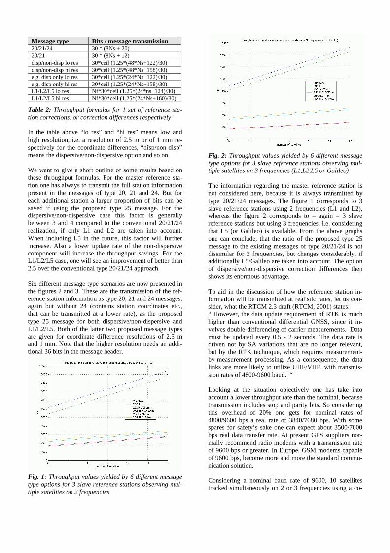
Six different message type scenarios are now presented inthe figures 2 and 3. These are the transmission of the ref-erence station information as type 20, 21 and 24 messages,again but without 24 (contains station coordinates etc.,that can be transmitted at a lower rate), as the proposedtype 25 message for both dispersive/non-dispersive andL1/L2/L5. Both of the latter two proposed message typesare given for coordinate difference resolutions of 2.5 mand 1 mm. Note that the higher resolution needs an addi-tional 36 bits in the message header.

Fig. 1: Throughput values yielded by 6 different messagetype options for 3 slave reference stations observing mul-tiple satellites on 2 frequencies

Fig. 2: Throughput values yielded by 6 different messagetype options for 3 slave reference stations observing mul-tiple satellites on 3 frequencies (L1,L2,L5 or Galileo)

The information regarding the master reference station isnot considered here, because it is always transmitted bytype 20/21/24 messages. The figure 1 corresponds to 3slave reference stations using 2 frequencies (L1 and L2),whereas the figure 2 corresponds to – again – 3 slavereference stations but using 3 frequencies, i.e. consideringthat L5 (or Galileo) is available. From the above graphsone can conclude, that the ratio of the proposed type 25message to the existing messages of type 20/21/24 is notdissimilar for 2 frequencies, but changes considerably, ifadditionally L5/Galileo are taken into account. The optionof dispersive/non-dispersive correction differences thenshows its enormous advantage.

To aid in the discussion of how the reference station in-formation will be transmitted at realistic rates, let us con-sider, what the RTCM 2.3 draft (RTCM, 2001) states:“ However, the data update requirement of RTK is muchhigher than conventional differential GNSS, since it in-volves double-differencing of carrier measurements. Datamust be updated every 0.5 - 2 seconds. The data rate isdriven not by SA variations that are no longer relevant,but by the RTK technique, which requires measurement-by-measurement processing. As a consequence, the datalinks are more likely to utilize UHF/VHF, with transmis-sion rates of 4800-9600 baud. “

Looking at the situation objectively one has take intoaccount a lower throughput rate than the nominal, becausetransmission includes stop and parity bits. So consideringthis overhead of 20% one gets for nominal rates of4800/9600 bps a real rate of 3840/7680 bps. With somespares for safety’s sake one can expect about 3500/7000bps real data transfer rate. At present GPS suppliers nor-mally recommend radio modems with a transmission rateof 9600 bps or greater. In Europe, GSM modems capableof 9600 bps, become more and more the standard commu-nication solution.

Considering a nominal baud rate of 9600, 10 satellitestracked simultaneously on 2 or 3 frequencies using a co-

ordinate difference resolution of 1 mm, results in a differ-ent number of slave reference stations, whose informationcan be transmitted in 1 second, using three different alter-natives. The following table shows the results using themessages a) 20/21/24, b) the proposed 25 in the disper-sive/non-dispersive option and c) the proposed 25 in theL1/L2/L5 option.

Number of Slave Reference Stations Using …Message Format L1+L2 L1+L2+L5a) RTCM 20/21/24 2 1b) dispersive/non-disp. 8 8c) L1/L2/L5 6 4

Table 3: Number of slave reference stations, that can betransmitted in 1 sec. at 9600 bps with 10 satellites trackedat 2 or 3 frequencies, using different message formats

Fig. 3: Throughput of slave reference stations for oneepoch, tracking 10 satellites at 2 frequencies, comparisonof different proposals

Note that the information of the master reference stationhas been omitted in this theoretical calculation. Consider-ing a third frequency, there is a problem in case a) totransmit more than the information of the master referencestation. This highlights the need of a new message formatfor the transmission of reference station network informa-tion.

The need to transmit the information of more than e.g.five reference stations leads to the discussion, how oftenthe station information should be updated (especiallyregarding the high-frequent changes of the dispersiveeffects) and which latency can be accommodated by therover processing software. This may result in the distribu-tion of the information related to one specific measure-ment epoch over a specific number of seconds. The likelydemand of transmitting the data of as many stations aspossible favorites the dispersive/non-dispersive option,because it allows the transmission of one component at alower rate. This will afford a great saving of bits and soallow the transmission of more stations’ data at the sametime.

CONCLUSIONS AND SUMMARY

A new message standard has been proposed to aid thesupport of reference network applications. Its use shouldovercome some of the problems seen in recent proposalsfor reference station network positioning concepts.

Our concept is based on transmitting messages of type20/21/24 for a master reference station and a newly pro-posed message type for further reference stations. Themore additional reference stations are transmitted usingthe proposed message type, the greater the savings arecompared to using RTCM messages of type 20,21 and 24.

The main advantages of the proposed message formats areas follows:§ There are less data bits to transmit in general§ The correction differences can be used for direct

interpolation, once adjusted to the common integerambiguity level

§ No detailed model specifications are needed (e.g. fortroposphere)

§ One-way communication is sufficient§ Kinematic applications can work without interrup-

tions and discontinuities unlike a VRS system, whichhas to change its VRS position during motion.

§ There are no restrictions on the number of users in areference station network

§ No dependency exists to a specific concept approach:The rover user gets the full reference station networkinformation and can independently use its own mod-els, interpolation and processing concepts

This approach can be used with update rates of up to 1 Hz,elevation masks down to 5° and reference station dis-tances up to 300 km.

With the implementation of L5, the dispersive/non-dispersive option will easily provide the most efficient useof throughput. Variations in the dispersive component willthen dictate the lower limit for the correction differenceupdates.

Further ConsiderationsIn addition to the issues raised in this paper, one has todiscuss some further:§ In the case of a third frequency one has possibly toconsider an additional correction residual for the proposeddispersive/non-dispersive option. This would be neces-sary, if really independent corrections or observations ofall three frequencies shall be reconstructed.§ “Static” information as the coordinates can be ex-tracted of the proposed message type and foreseen to betransmitted at a low rate. A therefore created extra mes-sage type format should include a network ID, the refer-ence stations’ IDs and coordinate differences. This wouldincrease the throughput.§ The coordinate differences of the slave referencestations could alternatively represented by latitude-, lon-gitude- and height differences related to one system refer-

ence ellipsoid (e.g. the WGS84). While a resolution in themillimeter level is necessary for the height, the resolutionof the horizontal components can be held at a lower level,possibly 2.5 m. This helps to save some bits and so toincrease the throughput.§ Suppose a larger number of slave reference stations.Their coordinate differences shall be transmitted in se-quence, but related to the same epoch. This possibly takeslonger than the update interval of the 20/21 messages ofthe master reference station, that are updated at a higherrate related then to more recent epochs. The potentiallyarising synchronization problems have to be discussed.Finally one can state, that the proposed concept can miti-gate or solve many of the problems of the existing con-cepts.

REFERENCES

Euler H.-J., Goad C.C. (1991): On optimal filtering ofGPS dual frequency observations without using orbitinformation. Bulletin Géodésique (1991) 65: 130-143, Springer-Verlag Berlin.

Han, S., Rizos, C. (1999): The impact of two additionalcivilian GPS frequencies on ambiguity resolutionstrategies. 55th National Meeting U.S. Institute ofNavigation, "Navigational Technology for the 21stCentury", Cambridge, Massachusetts, 28-30 June, pp.315-321.

Hatch, Jung, Enge, Pervan (2000): Civilian GPS: TheBenefits of Three Frequencies. GPS Solutions Volume3, Number 4, Spring 2000, pp. 1-9.

Jäggi A., G. Beutler, U. Hugentobler (2001): Using Dou-ble Difference Information from Network Solutions toGenerate Observations for a Virtual GPS ReferenceReceiver. Paper presented at the IAG 2001 ScientificAssembly, 2 - 7 September 2001 - Budapest, Hungary.

Large, Goddard, Landau (2001): eRTK: A New Genera-tion of Solutions for Centimeter-Accurate Wide-AreaReal-Time Positioning. Trimble Navigation Limited,Dayton, Ohio.

Rizos, C., Han, S., Chen, H.Y. (2000): Regional-scalemultiple reference stations for real-time carrier phase-based GPS positioning: a correction generation algo-rithm. Earth, Planets & Space, 52(10), pp. 795-800.

RTCM (2001): RTCM Recommended Standards forDifferential GNSS (Global Navigation SatelliteSystems) Service, First Committee Draft, FutureVersion 2.3, under development by RTCM SpecialCommittee No. 104, march 22, 2001.

Townsend B, K. Van Dierendonck, J. Neumann, I.Petrovski, S. Kawaguchi, and H. Torimoto(2000): A Proposal for Standardized Network RTKMessages. Paper presented at ION GPS 2000, SaltLake City.

Vollath U., A. Buecherl, H. Landau, C. Pagels, B.Wagner (2000/1): Multi-Base RTK PositioningUsing Virtual Reference Stations. Paper presented atION GPS 2000, Salt Lake City.

Wanninger (1994): Der Einfluß der Ionosphäre auf diePositionierung mit GPS. Wissenschaftliche Arbeitender Fachrichtung Vermessungswesen der UniversitätHannover Nr. 201.

Wanninger, L. (1999): The Performance of Virtual Ref-erence Stations in Active Geodetic GPS-Networksunder Solar Maximum Conditions. Proceedings ofION GPS 99, Nashville, S. 1419-1427.

Wübbena. G, A. Bagge, G. Seeber, V. Böder, P.Hankemeier (1996): Reducing Distance DependentErrors for Real-Time Precise DGPS Applications byEstablishing Reference Station Networks. Paper pre-sented at ION 96, Kansas City.

Wübbena, G., A. Bagge, M. Schmitz (2000): GPS-Referenznetze und internationale Standards. Vor-träge des 3. SAPOS-Symposium der Arbeitsgemein-schaft der Vermessungsverwaltungen der Länder derBundesrepublik Deutschland (AdV), 23.-24.Mai2000, München, Germany, pp. 14-23.

Wübbena. G., S. Willgalis (2001): State Space Approachfor Precise Real Time Positioning in GPS ReferenceNetworks. Presented at International Symposium onKinematic Systems in Geodesy, Geomatics andNavigation, KIS-01, Banff, June 5-8, Canada.

APPENDIX 1: PROPOSAL FOR A RTK NETWORK RTCM MESSAGE TYPE 25 FORMAT

These appendices are related to the formats and contents of the proposed Message Type 25 messages as described in the sec-tions above. Both the structures and the format examples have been created in a format identical to those detailed in RTCM2.3 (RTCM, 2001).

Table 1. PROPOSED MESSAGE TYPE 25 - RTK NETWORK CORRECTION DIFFERENCESDispersive/non-dispersive option, co-ordinate difference resolution 2.5 m or 1 mm

PARAMETER NUMBEROF BITS

SCALEFACTOR

AND UNITS

RANGE

GNSS TIME OFMEASUREMENT

3 0.1 s 0.0 to 0.5 s (See Note 1)

M = MULTIPLEMESSAGE INDICATOR

1 -- “0” – informs the receiver that this is the last message of thistype (proposed 25) having this time tag“1” – informs the receiver that another message of this type(proposed 25) with the same time tag will follow

GS = GLOBALSATELLITE SYSTEMINDICATOR (See Note 2)

2 -- “00” – Message is for GPS satellites“10” – Message is for GLONASS satellites“01” – Message is for GALILEO satellites“11” – reserved for future systems

NUMBER OF STATIONSTRANSMITTED

4 1 0 to 15 (See Note 3)

DIFFERENCINGSTATION ID

10 1 0 to 1023 (See Note 4)

ECEF DXCO-ORDINATE

18 2.5 m ±327677.5 m (See Note 5)

ECEF DYCO-ORDINATE

18 2.5 m ±327677.5 m (See Note 5)

ECEF DZCO-ORDINATE

18

S = 74

2.5 m ±327677.5 m (See Note 5)

* ECEF DXCO-ORDINATE

30 1 mm ±536870911 mm (See Note 5*)

* ECEF DYCO-ORDINATE

30 1 mm ±536870911 mm (See Note 5*)

* ECEF DZCO-ORDINATE

30

* S = 110

1 mm ±536870911 mm (See Note 5*)

P/C = CA-Code / P-CodeINDICATOR

1 -- "0" – C/A-Code"1" – P-Code

SATELLITE ID 6 1 0 to 63 (if GALILEO uses >32 SV IDs)DISPERSIVE OR NON-DISPERSIVEINDICATOR

1 -- "0" – Dispersive correction follows"1" – Non-dispersive correction follows(See Note 6)

CARRIER PHASECORRECTIONDIFFERENCE

16 1/256 cycle ±128 full cycles (See Note 7)

Total 24xNs+74* 24xNs+110

Coarse Co-ordinate Resolution* Fine Co-ordinate Resolution

PARITY Nx6

Note 1: GNSS TIME OF MEASUREMENT For this data slot only 2 bits are required, if a resolution of 1 Hz seems sufficientfor customers and suppliers (to be decided)

Note 2: GS – GLOBAL SYSTEM INDICATOR The anticipated presence of Europe’s GNSS GALILEO, and its additional sig-nals, in around 2008 should be kept in mind. GALILEO is expected to be a multiple frequency system also.

Note 3: NUMBER OF STATIONS TRANSMITTED A maximum of 15 stations has been assumed as an extreme value. Thisvalue may only be reached in high-density monitoring networks.

Note 4: DIFFERENCING STATION ID Analogously to the Master Station ID in the header

Note 5: DIFFERENCING STATION CO-ORDINATES: RESOLUTION DEPENDENT There are two levels proposed for theresolution of the differencing station co-ordinates, 2.5 meters and 1 millimeter respectively. The former resolutionwould assist the rover in its interpolation of correction differences whereas the latter would allow the rover to ‘recon-struct’ the measurements of each slave reference station.

Note 6: DISPERSIVE OR NON-DISPERSIVE INDICATOR Identifies whether the carrier phase correction difference messagecontains corrections for the dispersive or the non-dispersive component.

Note 7: CARRIER PHASE CORRECTION DIFFERENCE The carrier phase correction differences are represented in L1cycles for consistency. They are always related to the phase center, i.e. the Antenna Reference Point (ARP) of the ref-erence stations involved (analogous to message type 24) corrected by the model type antenna PCVs (e.g. a “nullan-tenna”); in any case their antenna phase center behaviour has to be consistent with that of the master reference sta-tion. At a resolution of 1/256 of a cycle, 16 bits allows a range of correction differences of ±128 full cycles. This cor-responds to ±25.3 meters in terms of L1 cycles.

Table 2. PROPOSED MESSAGE TYPE 25 - RTK NETWORK CORRECTION DIFFERENCESMultifrequency option, co-ordinate difference resolution 2.5 m or 1 mm


SCALEFACTOR

AND UNITS

RANGE

F = FREQUENCYINDICATOR

2 -- "00": L1 message"10": L2 message"01": L5 message"11": other(Galileo frequencies correspondingly)


3 0.1 s 0.0 to 0.5 s (See Note 1)






4 1 0 to 15 (See Note 3)


10 1 0 to 1023 (See Note 4)

ECEF DXCO-ORDINATE

18 2.5 m ±327677.5 m (See Note 5)

ECEF DYCO-ORDINATE

18 2.5 m ±327677.5 m (See Note 5)

ECEF DZCO-ORDINATE

18

S = 76

2.5 m ±327677.5 m (See Note 5)

* ECEF DXCO-ORDINATE

30 1 mm ±536870911 mm (See Note 5*)

* ECEF DYCO-ORDINATE

30 1 mm ±536870911 mm (See Note 5*)

* ECEF DZCO-ORDINATE

30

* S = 112

1 mm ±536870911 mm (See Note 5*)


1 -- "0" – C/A-Code"1" – P-Code

SATELLITE ID 6 1 0 to 63 (if GALILEO uses >32 SV IDs)


17 1/256 Cycle ±256 Full Cycles (See Note 7)

Total 24xNs+76* 24xNs+112

Coarse Co-ordinate Resolution* Fine Co-ordinate Resolution

PARITY Nx6

Note 1: GNSS TIME OF MEASUREMENT For this data slot only 2 bits are required, if a resolution of 1 Hz seems sufficientfor customers and suppliers (to be decided)

Note 2: GS – GLOBAL SYSTEM INDICATOR The anticipated presence of Europe’s GNSS GALILEO, and its additional sig-nals, in around 2008 should be kept in mind. GALILEO is expected to be a multiple frequency system also.

Note 3: NUMBER OF STATIONS TRANSMITTED A maximum of 15 stations has been assumed as an extreme value. Thisvalue may only be reached in high-density monitoring networks.

Note 4: DIFFERENCING STATION ID Analogously to the Master Station ID in the header

Note 5: DIFFERENCING STATION CO-ORDINATES: RESOLUTION DEPENDENT There are two levels proposed for theresolution of the differencing station co-ordinates, 2.5 meters and 1 millimeter respectively. The former resolutionwould assist the rover in its interpolation of correction differences whereas the latter would allow the rover to ‘recon-struct’ the measurements of each slave reference station.

Note 6: not used here

Note 7: CARRIER PHASE CORRECTION DIFFERENCE The carrier phase correction differences are represented in thecorresponding cycles for consistency. They are always related to the phase center, i.e. the Antenna Reference Point(ARP) of the reference stations involved (analogous to message type 24) corrected by the model type antenna PCVs(e.g. a “nullantenna”); in any case their antenna phase center behaviour has to be consistent with that of the masterreference station. At a resolution of 1/256 of a cycle, 17 bits allows a range of correction differences of ±256 full cy-cles. This corresponds to ±50.6 meters in terms of L1 cycles.

Figure 1. PROPOSED MESSAGE TYPE 25 - RTK NETWORK CORRECTION DIFFERENCESDispersive/non-dispersive option, co-ordinate difference resolution 2.5 m

FIRST TWO WORDS OF HEADER - (RTCM agreed standard) transmitted at the beginning of the message string

1 2 3 4 5 6 7 8 9 10 11 12 13 14 15 16 17 18 19 20 21 22 23 24 25 26 27 28 29 30

MESSAGE TYPE MASTER REFERENCE

1 PREAMBLE PARITY Word 1(FRAME ID) STATION ID

1 2 3 4 5 6 7 8 9 10 11 12 13 14 15 16 17 18 19 20 21 22 23 24 25 26 27 28 29 30

SEQUENCE NUMBER OF STATION2 MODIFIED Z-COUNT PARITY Word 2

NUMBER DATA WORDS HEALTH

THIRD TO 6TH WORD - transmitted at the beginning of the Type 25 message and includes satellite-independent data

1 2 3 4 5 6 7 8 9 10 11 12 13 14 15 16 17 18 19 20 21 22 23 24 25 26 27 28 29 30

GNSS # OF STNS ECEF DX3 TIME OF M G S DIFFERENCING STATION ID PARITY Word 3

MMENT TRANSMITTED CO-ORD

1 2 3 4 5 6 7 8 9 10 11 12 13 14 15 16 17 18 19 20 21 22 23 24 25 26 27 28 29 30

ECEF DX ECEF DY4 PARITY Word 4

CO-ORDINATE (CONT) CO-ORDINATE

1 2 3 4 5 6 7 8 9 10 11 12 13 14 15 16 17 18 19 20 21 22 23 24 25 26 27 28 29 30

ECEF DY ECEF DZ5 CO-ORDINATE PARITY Word 5

(CONT) CO-ORDINATE

1 2 3 4 5 6 7 8 9 10 11 12 13 14 15 16 17 18 19 20 21 22 23 24 25 26 27 28 29 30

ECEF DZ6 CO-ORD FILL / SPARE PARITY Word 6

(CONT)

EACH SATELLITE - 1 WORD for the Dispersive as well as for the Non-dispersive component

1 2 3 4 5 6 7 8 9 10 11 12 13 14 15 16 17 18 19 20 21 22 23 24 25 26 27 28 29 30

SATELLITE D/ CARRIER PHASEP-C PARITY Word Ns + 6

ID N-D CORRECTION DIFFERENCE (L1 cycles)

Figure 2. PROPOSED MESSAGE TYPE 25 - RTK NETWORK CORRECTION DIFFERENCESMultifrequency option, co-ordinate difference resolution 2.5 m


1 2 3 4 5 6 7 8 9 10 11 12 13 14 15 16 17 18 19 20 21 22 23 24 25 26 27 28 29 30



1 2 3 4 5 6 7 8 9 10 11 12 13 14 15 16 17 18 19 20 21 22 23 24 25 26 27 28 29 30

SEQUENCE NUMBER OF STATION

2 MODIFIED Z-COUNT PARITY Word 2NUMBER DATA WORDS HEALTH

THIRD TO 6TH WORD - transmitted at the beginning of the proposed type message and includes satellite-independent data

1 2 3 4 5 6 7 8 9 10 11 12 13 14 15 16 17 18 19 20 21 22 23 24 25 26 27 28 29 30

GNSS # OF STNS ECEF3 F TIME OF M G S DIFFERENCING STATION ID DX PARITY Word 3

MMENT TRANSMITTED CO-ORD

1 2 3 4 5 6 7 8 9 10 11 12 13 14 15 16 17 18 19 20 21 22 23 24 25 26 27 28 29 30

ECEF DX ECEF DY

4 PARITY Word 4CO-ORDINATE (CONT) CO-ORDINATE

1 2 3 4 5 6 7 8 9 10 11 12 13 14 15 16 17 18 19 20 21 22 23 24 25 26 27 28 29 30

ECEF DY ECEF DZ

5 CO-ORDINATE PARITY Word 5(CONT) CO-ORDINATE

1 2 3 4 5 6 7 8 9 10 11 12 13 14 15 16 17 18 19 20 21 22 23 24 25 26 27 28 29 30

ECEF DZ

6 CO-ORD FILL / SPARE PARITY Word 6(CONT)

EACH SATELLITE - 1 WORD corresponding to the relevant frequency specified in WORD 3

1 2 3 4 5 6 7 8 9 10 11 12 13 14 15 16 17 18 19 20 21 22 23 24 25 26 27 28 29 30

SATELLITE CARRIER PHASEP-C PARITY Word Ns + 6

ID CORRECTION DIFFERENCE (L1)

Figure 3. PROPOSED MESSAGE TYPE 25 - RTK NETWORK CORRECTION DIFFERENCESDispersive/non-dispersive option, co-ordinate difference resolution 1 mm


1 2 3 4 5 6 7 8 9 10 11 12 13 14 15 16 17 18 19 20 21 22 23 24 25 26 27 28 29 30



1 2 3 4 5 6 7 8 9 10 11 12 13 14 15 16 17 18 19 20 21 22 23 24 25 26 27 28 29 30




1 2 3 4 5 6 7 8 9 10 11 12 13 14 15 16 17 18 19 20 21 22 23 24 25 26 27 28 29 30

GNSS # OF STNS ECEF DX

3 TIME OF M G S DIFFERENCING STATION ID PARITY Word 3MMENT TRANSMITTED CO-ORD

1 2 3 4 5 6 7 8 9 10 11 12 13 14 15 16 17 18 19 20 21 22 23 24 25 26 27 28 29 30

ECEF DX

4 PARITY Word 4CO-ORDINATE (cont)

1 2 3 4 5 6 7 8 9 10 11 12 13 14 15 16 17 18 19 20 21 22 23 24 25 26 27 28 29 30

ECEF DX ECEF DY5 CO-ORD PARITY Word 5

(cont) CO-ORDINATE

1 2 3 4 5 6 7 8 9 10 11 12 13 14 15 16 17 18 19 20 21 22 23 24 25 26 27 28 29 30

ECEF DY ECEF DZ6 PARITY Word 6

CO-ORDINATE (cont) CO-ORDINATE

1 2 3 4 5 6 7 8 9 10 11 12 13 14 15 16 17 18 19 20 21 22 23 24 25 26 27 28 29 30

ECEF DZ7 FILL / SPARE PARITY Word 7

CO-ORDINATE (cont)

EACH SATELLITE - 1 WORD for the Dispersive as well as for the Non-dispersive component

1 2 3 4 5 6 7 8 9 10 11 12 13 14 15 16 17 18 19 20 21 22 23 24 25 26 27 28 29 30

SATELLITE D/ CARRIER PHASEP-C PARITY Word Ns + 7

ID N-D CORRECTION DIFFERENCE (L1 cycles)

Figure 4. PROPOSED MESSAGE TYPE 25 - RTK NETWORK CORRECTION DIFFERENCESMultifrequency option, co-ordinate difference resolution 1 mm


1 2 3 4 5 6 7 8 9 10 11 12 13 14 15 16 17 18 19 20 21 22 23 24 25 26 27 28 29 30



1 2 3 4 5 6 7 8 9 10 11 12 13 14 15 16 17 18 19 20 21 22 23 24 25 26 27 28 29 30




1 2 3 4 5 6 7 8 9 10 11 12 13 14 15 16 17 18 19 20 21 22 23 24 25 26 27 28 29 30

GNSS # OF STNS ECEF

3 F TIME OF M G S DIFFERENCING STATION ID DX PARITY Word 3MMENT TRANSMITTED CO-ORD

1 2 3 4 5 6 7 8 9 10 11 12 13 14 15 16 17 18 19 20 21 22 23 24 25 26 27 28 29 30

ECEF DX

4 PARITY Word 4CO-ORDINATE

1 2 3 4 5 6 7 8 9 10 11 12 13 14 15 16 17 18 19 20 21 22 23 24 25 26 27 28 29 30

ECEF DX ECEF DY

5 CO-ORD PARITY Word 5(cont) CO-ORDINATE

1 2 3 4 5 6 7 8 9 10 11 12 13 14 15 16 17 18 19 20 21 22 23 24 25 26 27 28 29 30

ECEF DY ECEF DZ

6 PARITY Word 6CO-ORDINATE (cont) CO-ORDINATE

1 2 3 4 5 6 7 8 9 10 11 12 13 14 15 16 17 18 19 20 21 22 23 24 25 26 27 28 29 30

ECEF DZ7 FILL / SPARE PARITY Word 7

CO-ORDINATE (cont)

EACH SATELLITE - 1 WORD corresponding to the relevant frequency specified in WORD 3

1 2 3 4 5 6 7 8 9 10 11 12 13 14 15 16 17 18 19 20 21 22 23 24 25 26 27 28 29 30

SATELLITE CARRIER PHASEP-C PARITY Word Ns + 7

ID CORRECTION DIFFERENCE (L1)

APPENDIX 2: ALTERNATIVELY PROPOSED MESSAGE TYPES (25/26) LAYOUT

Includes: Split-up of Static Information and Latitude-/Longitude-/Height-Differences with Optimized ResolutionTables only, no message scheme graphs

Table 1. PROPOSED MESSAGE TYPE 25 - RTK NETWORK CORRECTION DIFFERENCESDispersive/non-dispersive option


SCALEFACTOR

AND UNITS

RANGE


3 0.1 s 0.0 to 0.5 s (See Note 1)





NETWORK ID 5 1 0 to 31NUMBER OF STATIONSTRANSMITTED

4 1 0 to 15


10 1 0 to 1023


1 -- "0" – C/A-Code"1" – P-Code

SATELLITE ID 6 1 0 to 63 (if GALILEO uses >32 SV IDs)DISPERSIVE OR NON-DISPERSIVEINDICATOR

1 -- "0" – Dispersive correction follows"1" – Non-dispersive correction follows


16 1/256 cycle ±128 full cycles

Total 24xNs+25PARITY Nx6

Note: The Header always contains the Master Reference Station ID; this avoids the implementation of a network ID.

Table 2.1 PROPOSED MESSAGE TYPE 26 - RTK NETWORK DEFINITIONOption 1: Cartesian ECEF Coordinate Differences, Resolution 2.5 m


SCALEFACTOR

AND UNITS

RANGE




4 1 0 to 15


10 1 0 to 1023

ECEF DXCOORDINATE

18 2.5 m ±327677.5 m

ECEF DYCOORDINATE

18 2.5 m ±327677.5 m

ECEF DZCOORDINATE

18

S = 64

2.5 m ±327677.5 m

Total 64xNsref+5 Coarse Coordinate ResolutionNsref = Number of Slave Reference Stations

PARITY Nx6


Table 2. 2 PROPOSED MESSAGE TYPE 26 - RTK NETWORK DEFINITIONOption 2: Cartesian ECEF Coordinate Differences, Resolution 1 mm


SCALEFACTOR

AND UNITS

RANGE




4 1 0 to 15


10 1 0 to 1023

ECEF DXCOORDINATE

30 1 mm ±536870911 mm

ECEF DYCOORDINATE

30 1 mm ±536870911 mm

ECEF DZCOORDINATE

30

S = 100

1 mm ±536870911 mm

Total 100xNsref+5 Fine Coordinate ResolutionNsref = Number of Slave Reference Stations

PARITY Nx6


Table 2. 3 PROPOSED MESSAGE TYPE 26 - RTK NETWORK DEFINITIONOption 3: Ellipsoidal ECEF Coordinate Differences, Resolution 0.000025 deg in Lat. and Lon., 1mm in height


SCALEFACTOR

AND UNITS

RANGE




4 1 0 to 15


10 1 0 to 1023

WGS84 DLATCOORDINATE

18 0.000025 deg ±3.2767 degrees (corresponds to a resolution of alwaysbetter than 2.7 m)

WGS84 DLONCOORDINATE

19 0.000025 deg ±6.5535 degrees (double as DLAT due to high latitude ap-plications: at a latitude=60 deg the maximum distance inlongitude shortens down to the same of DLAT, i.e. about 350km; at a latitude=70 deg down to about 240 km)

WGS84 DHGTCOORDINATE

22

S = 69

1 mm ±2097.151 m (Height above WGS84 Ellipsoid in an ITRFConformed Reference Frame, like the GPS )

Total 69xNsref+5 WGS84 Ellipsoidal Coordinates, Coarse Latitude/Longitude,Fine Height ResolutionNsref = Number of Slave Reference Stations

PARITY Nx6

Note: The WGS84 DLAT, DLON, DHGT option can also be used to generate a grid of reference stations

Note: The WGS84 DHGT option is set to a finer resolution due to height sensitivity of atmospheric refraction correction

Note: The WGS84 DLAT, DLON, DHGT option uses the same datum definition (e.g. an ITRF realization) as the master refer-ence station, but it is always referenced to the surface of the WGS84 ellipsoid


APPENDIX 3: COMPARISON OF THE EXISTING AND THE PROPOSED NETWORK MESSAGES

Table 1: NETWORK MESSAGESMESSAGETYPE NO.

MESSAGE NAME # OF BITS

20 CARRIER PHASE CORRECTIONS 30 * (2Ns + 3)21 PSEUDORANGE CORRECTIONS 30 * (2Ns + 3)24 ANTENNA REFERENCE POINT (ARP) 30 * (8)

proposed 25 / 25+26 CARRIER PHASE CORRECTION DIFFERENCES depends on decision

Table 2: NETWORK MESSAGES – ACTUAL STATUSMESSAGETYPE NO.


20 CARRIER PHASE CORRECTIONS L1 + L2 30 * (4Ns + 6)21 PSEUDORANGE CORRECTIONS L1 + L2 30 * (4Ns + 6)24 ANTENNA REFERENCE POINT (ARP) 30 * (8)

SUM OF 1 SET OF ADDITIONAL REFERENCE STATION CORRECTIONS 30 * (8Ns + 20)SUM OF 1 SET OF ADDITIONAL REFERENCE STATION CORRECTIONS,

UPDATE WITHOUT MESSAGE TYPE 24 INFORMATION30 * (8Ns + 12)

Table 3: PROPOSED NETWORK MESSAGE TYPE 25 (DISPERSIVE/NON-DISPERSIVE OPTION)MESSAGETYPE NO.


CARRIER PHASE CORRECTION DIFFERENCES: HEADER 122 + parity

1 BODY TYPE DISPERSIVE COMPONENT (PER SAT.) 24Ns + parity

25 proposed(DISP /

NONDISP)

1 BODY TYPE NON-DISPERSIVE COMPONENT (PER SAT.) 24Ns + parity

SUM OF 1 SET OF ADDITIONAL REFERENCE STATION CORRECTIONS 30*ceil (1.25*(48*Ns+122)/30)

SUM OF 1 SET OF ADDITIONAL REFERENCE STATION CORRECTIONS, BUTONLY UPDATE OF ONE OF THE COMPONENTS

30*ceil (1.25*(24*Ns+122)/30)

SUM OF 1 SET OF ADD. REF. STAT. CORR., HI-RES COORD. DIFF 30*ceil (1.25*(48*Ns+158)/30)

SUM OF 1 SET OF ADD. REF. STAT. CORR., HI-RES COORD. DIFF, BUT ONLY UPDATE OF ONE OF THE COMPONENTS

30*ceil (1.25*(24*Ns+158)/30)

Table 4: PROPOSED NETWORK MESSAGE TYPE 25 (MULTIFREQUENCY OPTION)MESSAGETYPE NO.


25 proposed(L1 / L2 / L5)

CARRIER PHASE CORRECTION DIFFERENCES L1 or L2 or L5 24Ns + 124 + parity

SUM OF 1 SET OF ADDITIONAL REFERENCE STATION CORRECTIONS,DEPENDENT ON THE # OF FREQUENCIES AVAILABLE

Nf*30*ceil (1.25*(24*Ns+124)/30)

SUM OF 1 SET OF ADDITIONAL REFERENCE STATION CORRECTIONS, DEP.ON THE # OF FREQ. AVAILABLE, HI-RES COORD. DIFF.

Nf*30*ceil (1.25*(24*Ns+160)/30)

Table 5: PROPOSED NETWORK MESSAGE TYPES 25 AND 26 (DISPERSIVE/NON-DISPERSIVE OPTION)MESSAGETYPE NO.


25 proposed RTK NETWORK CORRECTION DIFFERENCES (dispersive or non-dispersive) 30*ceil (1.25*(24*Ns+25)/30)

26 proposed RTK NETWORK DEFINITION (DLAT, DLON, DHGT option) 30*ceil (1.25*(69*Nsref+5)/30)

The factor of 1.25 is due to the relation of data and parity bits. To take the fill spares into account the 30 bits words are rounded up by the“ceil” function.“HI-RES” means high resolution, i.e. a 1 mm resolution in comparison to the other treated case of 2.5 m

Figures: THROUGHPUT OF THE EXISTING AND THE PROPOSED NETWORK MESSAGESINCLUDING THE OPTION OF SPLITTING UP THE STATIC INFORMATION (25/26)

Fig. 1: Throughput for the 1st epoch, comparison of different proposals; the 25/26 option shows some advantage from thesecond epoch on: one saves 270 bits regarding 3 slave reference stations, independent from the number of satellites.

Fig. 2: Throughput for one epoch, comparison of different proposals; the 25-spit/without-26-option shows some advantage,but there is no distinct improvement. The three lowest lines (25/disp/2.5m, 25/26split_option, 25w/o26split_option) base all onthe dispersive/non-dispersive concept and reduce furthermore, if one of the components will be transmitted on a slower ratedue to a smoother error behaviour with time.

APPENDIX 4: Issues for Discussion

§ Methods of Data Transmission, Latency Aspects:Under the simplified approach proposed here, the network RTK corrections, i.e. RTCM 20/21/24 of the master reference sta-tion and the proposed type 25 from all slave reference stations, would be transmitted to users in the area of the network stationsconcerned. This could be done sequentially or in parallel. This discussion is better visualised if one considers a favourablenetwork operating scenario; e.g. a network of n dual-frequency reference stations approximately 300 kilometres apart support-ing a number of roving users.

In a sequential station by station approach, the correction differences for only one slave reference station per related epochwould be transmitted. For this example of n stations, the correction difference information could be transmitted in just n ep-ochs after which the transmission cycle is repeated again. So the information of the first station transmitted is related to onemeasurement epoch, the information of a second station is related to the next following epoch then, and so on …If the modem’s baud rate is high enough (and the throughput small enough), the rover may be able to support the parallelreceipt of data relating to more than say, two stations, but related to the same epoch. This transmission can cover the span oftime allowed as latency.

Due to this one has to consider and discuss the effects of latency, the problems of extrapolation in time or the possibility touse the information of two consecutive epochs enabling temporal interpolation.

§ Dispersive/Non-Dispersive Option and a Third Frequency:In the case of a third frequency one has possibly to consider an additional correction residual for the proposed dispersive/non-dispersive option. This would be necessary, if really independent corrections or observations of all three frequencies shall bereconstructed.

§ Extra Message for Static Information:“Static” information can be drawn out of the proposed message type and foreseen to be transmitted at a low rate. A thereforecreated extra message type format should include a network ID, the reference stations’ IDs and coordinate differences. Thiswould increase the throughput.

§ Coordinate Difference Representation and Resolution:The coordinate differences of the slave reference stations could alternatively represented by latitude-, longitude- and heightdifferences related to one system reference ellipsoid (e.g. the WGS84). While a resolution in the millimeter level is necessaryfor the latter one, the resolution of the first two can be held at a lower level, possibly 2.5 m. This helps to save some bits and soto increase the throughput.

§ Time Synchronization – Possible Backward Jumping of Z-Counts:Suppose a larger number of slave reference stations, whose coordinate difference messages shall be transmitted in sequence,but related to the same epoch. This possibly lasts longer than the update interval of the 20/21 messages of the master referencestation, that are updated at a higher rate related then to more recent epochs. The possibly arising synchronization problemshave to be discussed. For sequencing the frames, there was a sequence number introduced and the modified Z-Count should berelated directly to the measurement. The RTCM Doc V.2.3 defines, regarding the modified Z-Count:“In the case of non-pseudolite type transmission, it is the reference time for the message parameters only.”“The sequence number aids in frame synchronization for non-pseudolite type transmissions, replacing the sequencing Z-countas an incrementing parameter.”“GPS time is provide to the nearest 0.6 seconds in each message using the modified Z-count, although it should be remem-bered that the modified Z-count is referenced to the time of the correction, not the time at which the receiver has decoded themessage.”“The GNSS TIME OF MEASUREMENT shall be an estimate of GNSS time at the time of measurement.”

§ Ambiguity Level Indicator:One has to think about including an ambiguity level indicator into the proposed message type. This can be used e.g. to provideinformation about the ambiguity fixing status in the processed network area.

APPENDIX 5: DERIVATION OF THE DISPERSIVE/NON-DISPERSIVE CORRECTIONS

A linear combination is formed by2211 Φ⋅+Φ⋅=Φ ii [cycles] (A1)

for that the factors 1i and 2i have to be chosen. If onewants to get a ionosphere-free linear combination repre-senting the non-dispersive effect, one has to set

122 ffi −= . (A2)The wavelength is defined by

1221

21

λλλλ

λ⋅+⋅

⋅=

ii . (A3)

If the wavelength shall become equal to that of L1, one cansolve the equation (A3) for 1i considering (A2) and gets

−= 1

1

2212 λλλ

ff

i

and from that

2

22

1

21

11

22

21

ff

f

ff

i−

=−

=λλ

λ

as well as from (A2)

21

22

212

22

1

212

ff

ff

ff

ffi

−

⋅=

−

⋅−= .

For a geometry-free linear combination representing thedispersive effect one has to solve the equation

2211122

21

2211 1 λλλλ ⋅−⋅+⋅

−=⋅Φ−⋅Φ NNI

f

f(A4)

for 1I , which represents the ionospheric path delay on L1in meters. If the ambiguities 21 , NN are known and re-duced, one gets for the ionospheric path delay on L1, ex-pressed in L1 cycles

21

22

22

22

11

22

21

22

11

1

1

1

1

ff

fff

f

fffI

−⋅

Φ−Φ=

−

⋅

Φ−Φ=

λ

Proof:The sum of the above derived two components have toresult in the whole (dispersive plus non-dispersive) effecton L1:

1122

21

22

21

222

21

2112

22

1

21

222

21

2112

22

1

22

11

Φ=Φ−

−=

=Φ−

⋅−Φ

−+

+Φ−

⋅+Φ

−−

=Φ+Φ −

ff

ff

ff

ff

ff

f

ff

ff

ff

f

dispnondisp δδ

(A5)

q.e.d.

Sometimes the geometry-free as well as the ionosphere-free linear combination were derived without expressingthem in L1 cycles and without relating the dispersive ef-fect to the L1 frequency. The most common of the alterna-

tives neglect the factors in front jRTCMAB ,1,∆Φδ . But these

can reach

55.12

22

1

22 −≅−

−ff

f and

55.22

22

1

21 +≅−

+ff

f respectively.

This has to be considered.

One can also perform the proof of equation (A5) by usingthe equations (7) and (8) of the proposal paper, where theobservables are not related to [cycles], but to [meters]:

jRTCMAB

jRTCMAB

dispjRTCMAB

ff

f

ff

f

,2,21

22

22

,1,21

22

22,

,1,

∆Φ−

−

∆Φ−

=∆Φ

δ

δδ

(7)

jRTCMAB

jRTCMAB

dispnonjRTCMAB

ff

f

ff

f

,2,22

21

22

,1,22

21

21,

,1,

∆Φ−

−

∆Φ−

=∆Φ −

δ

δδ

(8)

Then we get:

jRTCMAB

jRTCMAB

jRTCMAB

jRTCMAB

jRTCMAB

jRTCMAB

dispnonjAB

dispjAB

ff

ff

ff

f

ff

f

ff

f

ff

f

,1,,1,22

21

22

21

,2,22

21

22

,1,22

21

21

,2,21

22

22

,1,21

22

22

,1,

,1,

∆Φ=∆Φ−

−=

=∆Φ−

−∆Φ−

+

+∆Φ−

−∆Φ−

=∆Φ+∆Φ −

δδ

δδ

δδ

δδ

q.e.d.

Please note, that although the non-dispersive term is nowindependent from wavelengths, the dispersive part is alsoexpressed in the units [meter], but has to be related to afrequency, in our case to L1, because the amount is fre-quency dependent.

Documents

Study of a Simplified Approach in Utilizing Information from Permanent Reference ... · 2016-12-15 · Utilizing Information from Permanent Reference Station Arrays H.-J. Euler,