Embed Size (px)
Citation preview
1
Studies On Falling Ball Viscometry
Amit Vikram Singh1, Lavanjay Sharma
2, and Pinaki Gupta-Bhaya
1
Departments of Chemistry1, Material Science Programme
2, Indian Institute of Technology Kanpur, Kanpur 208016
India
Abstract: A new method of accurate calculation of the coefficient of viscosity of a test liquid from experimentally measured
terminal velocity of a ball falling in the test liquid contained in a narrow tube is described. The calculation requires the value of a
multiplicative correction factor to the apparent coefficient of viscosity calculated by substitution of terminal velocity of the
falling ball in Stokes formula. This correction factor, the so-called viscosity ratio, a measure of deviation from Stokes limit, arises
from non-vanishing values of the Reynolds number and the ball/tube radius ratio. The method, valid over a very wide range of
Reynolds number, is based on the recognition of a relationship between two measures of wall effect, the more widely
investigated velocity ratio, defined as the ratio of terminal velocity in a confined medium to that in a boundless medium and
viscosity ratio. The calculation uses two recently published correlation formulae based on extensive experimental results on
terminal velocity of a falling ball. The first formula relates velocity ratio to Reynolds number and ball-tube radius ratio. The
second formula gives an expression of the ratio of the drag force actually sensed by the ball falling in an infinite medium to that
in the Stokes limit as a function of Reynolds number alone. It is shown that appropriate use of this correction factor extends the
utility of the technique of falling ball viscometry beyond the very low Reynolds number ‗creepy flow‘ regime, to which its
application is presently restricted. Issues related to accuracy are examined by use of our own measurements of the terminal
velocity of a falling ball in a narrow tube and that of published literature reports, on liquids of known viscosity coefficient.
1. Introduction
1.1 Evaluation of hydrodynamic forces on a rigid body in relative motion in a fluid has been of interest for a very
long time (Clift et. al [1], Happel and Brenner [2], Kim and Karrila 2005 [3]) and also recently (Leach 2009 [4]). A
falling spherical ball, which senses this force, has been used as a probe to study fluid properties. Measurement of
terminal velocity ( ) of a ball falling in a viscous fluid enclosed in a narrow tube provides a method for
determination of the coefficient of viscosity ( ) of the test liquid. This simple, yet accurate technique, in use for a
long time, is of considerable recent interest (Kahle et. al. [5], Kaiser et. al. [6], Brizard et. al. [7], Feng et. al. [8], Ma
et. al. [9]). A falling ball viscometer is commercially available and has been used for testing petroleum products,
pharmaceutical beverages, silicate glass and food products.
2
In addition to viscometry, study of a falling ball is important in several engineering domains which involve
multiphase flows e.g., sedimentation, improvement of combustion, minimization of erosion by droplets in large
turbines, hydrodynamic chromatography, membrane transport, hydraulic and pneumatic transport of coarse particles
in pipes, effects that utilize electric fields to enhance transport phenomena and separations in multiphase systems
(Kaji et. al. [10], Scott and Wham [11], Ptasinski and Kerkhof [12]).
Motion of a falling ball in a liquid contained in a narrow tube, apart from viscometry and other practical
applications, is interesting in its own right. Eccentric fall, horizontal wall forces, and accelerated pre-steady state fall
are a few examples of many interesting aspects of the physics of a falling ball (Happel and Brenner [2], Mordant and
Pinton [13], Tozeren [14], Rubinow and Keller [15], Shinohara and Hashimoto [16], Ambari et. al. [17], Humphrey
and Murata [18], Becker and Mc Kinley [19], Bougas and Stamatoudis [20], Feng et. al. [21], Changfu et. al. [22]).
Falling ball viscometry assumes importance in the study of non-Newtonian fluids, an area of considerable
recent interest. The use of more conventional viscometers, e.g., capillary or rotary, for zero-shear rate viscosity
measurement of non-Newtonian fluids is error-prone. Measurements at low shear rate are problematic in these
instruments and extrapolation to zero shear rate is ambiguous. Falling ball viscometer is superior in this regard and
considerable amount of work has been done in application of falling ball viscometry to measurement of viscosity of
non-Newtonian fluids, both experimental and in respect of techniques of extrapolation to zero shear stress (Kaiser et.
al. [6],Williams [23], Sutterby [24], Turian [25], Caswell [26], Cygan and Caswell [27], Subbaraman et. al. [28],
Chhabra and Uhlherr [29], Barnes [30], [31]).
1.2 Velocity ratio: A ball falling under the force of gravity in a fluid attains a terminal steady velocity when the
frictional (drag) force exactly balances the sum of oppositely directed force of gravity and force due to
buoyancy. This sum and therefore, the drag force on the ball in its state of steady fall, are determined by the ball-
fluid combination alone. Its magnitude is entirely independent of the presence or absence of the walls of the tube in
the vicinity of the falling ball. Drag force is a function of ball velocity. Although the numerical value of is
independent of the proximity of the ball with respect to the wall, its functional relation with is not. A ball liquid
combination with a given will show a tube diameter dependent . The magnitude of in an unbounded medium
is determined entirely by the ball fluid combination and that in a confined medium is determined, in addition, by the
location of the falling ball with respect to the wall. The value of in an infinite medium, designated and the
dimensionless Reynolds number (Eq. 2) that quantifies inertial effect and is proportional to are
characteristic parameters of the ball-liquid combination under test. The parameter that quantifies proximity of the
ball to the wall for centerline fall is the ratio of ball diameter to tube diameter, designated . The modification of
terminal velocity on confinement quantified by the ratio is a function of , the functional dependence being
parametrically dependent on the ball-liquid specific parameter . There exists extensive literature on
measurements and parameterization of as a function of and (Chhabra [32], DiFelice [33], Kehlenbeck
and DiFelice [34], Francis [35], Fidleris and Whitmore [36]; henceforth referred to as F&W), McNown [37]).

3
1.3 Viscosity ratio: Falling ball viscometry: In the limiting case of a boundless fluid medium ( ) and a
negligible inertial effect ( << 1) Stokes equation specifies the dependence of on , a linear function
(1)
denotes coefficient of dynamic viscosity of the fluid, r is ball radius and is defined by
(2)
where is liquid density and d is ball diameter
If one makes the unjustified assumption that Stokes equation holds in a narrow tube, one can calculate
from experimentally determined with use of the expression of in terms of physical parameters of the ball and
the liquid. Deviation from Stokes equation is accommodated by defining an apparent so-called Stokes coefficient of
viscosity in the structure of Stokes equation. The ratio (>1) designated viscosity ratio, is a measure of
deviation from Stokes equation. The expression of in terms of and physical parameters of the ball and the
liquid is given by
(3)
where is ball density, is fluid density, is acceleration due to gravity, and is ball radius. One can determine
for a test liquid from measured and then from a knowledge of .
Sutterby [38] reports experimental values of for equally spaced values of ( ), and
closely spaced small values of Reynolds number and measures of inertial
effects defined as follows
(4)
(5)
Whereas is characteristic of ball-liquid combination alone, and are also determined by through its
effect on . The three Reynolds numbers are equal in a boundless medium; and in a narrow tube are less
than for the same ball liquid pair. The ratio , shown to be a function of and alone, are calculated at
equally spaced values of and by interpolation of extensive experimental data for a wide variety of ball-liquid-
tube combination. is calculated from experimental values of in a falling ball viscometer and is measured in
4
an independent viscometer. The lack of information on as a function of Reynolds number over the whole
range is the only limiting factor in the use of falling ball viscometry to determination of absolute value of .
If measurements on for a given test liquid could be restricted to low Reynolds number regime covered
by Sutterby‘s work, falling ball viscometry would be applicable to any liquid. It may however, not be possible to
abide by this restriction in all situations. In falling ball experiments one has restriction on ball radius imposed by
experimental convenience of position detection and restriction on ball density by the requirement that it must exceed
the density of the test liquid as well as commercial availability. With these restrictions varies within a range. The
consequence of this restricted range is that low Reynolds number ―creepy flow‖ regime may not always be easy to
achieve, particularly for liquids of low viscosity. We consider this issue in sec. 4.1.1.
One way to extend the applicability of falling ball viscometry beyond the range covered by Sutterby [38] is
to extend measurements of that he reports to a wider range of . This is a tall order. However, extensive data
on , already exists over the whole range of and a very wide range of . Both of these ratios are measures
of deviation from Stokes equation. They are equal only in the limit . The relation between the two ratios can
be used for using velocity ratio data for calculation of viscosity ratio, well beyond the ‗creepy flow‘ regime.
The unavailability of viscosity ratio data at large has restricted the use of falling ball viscometry to the ‗creepy
flow‘ regime. Several very recent studies on falling ball viscometry (Kahle et. al. [5], Brizard et. al. [7] and Ma et.
al. [9]) are also restricted to low regime. We are not aware of its application to larger regime, where
does not equal .
1.4 Force ratio: We define a third measure of deviation from Stokes limit, the so called force ratio, and discuss its
relation to the two measures already defined.
If the conditions for validity of Eq. 1 do not hold, then the expression on R.H.S. of Eq. 1 no longer gives
the drag force and functional dependence of on is no longer linear. This expression, as a limiting force still
remains a part of description of the phenomena we study. A symbol is assigned to it. It represents Stokes limit for
a given terminal velocity. We define
(6)
If conditions of validity of Stokes equation hold .
The deviation of this ratio from unity in an infinite medium arises from a non negligible . In a confined
medium is an additional source of deviation. Deviation from Stokes limit implies nonlinear functional
dependence of on or as the case may be. being a linear function, is, in unbounded and in
confined medium, a non linear function of . The functional dependence of in an unbounded medium
5
( ) on has been specified in terms of the dimensionless , in the form of a power series using
perturbation theory (Proudman and Pearson [39]) and also by parameterization of extensive experimental results on
(Clift et. al. [1] and Cheng et. al. [40]). In a confined medium is independent, but being proportional to
is not; as a result is a function of as well as . This functional dependence has been studied using
computer simulation results (Wham et. al. [41]). Purely theoretical evaluation of a limiting force ratio
has received attention for more than a century (Happel and Brenner [2]a). The theories have been classified as
‗exact‘ and ‗approximate‘. Results of the former category are given in the form of tables (Tozeren [14], Haberman
[42], Payne and Scherr [43], Coutanceau [44], Bohlin [45]) and those of the latter are given in the form of a compact
function of (Haberman and Sayre [46]).
Number of reports on direct force measurements on suspended spheres to determine is not large.
Ambari et. al. [17], [47] use a magnetic rheometer to accurately measure force ratio at very low Reynolds number
( ).The results of ‗exact‘ theory are found to be in complete agreement with the experimenmtal results of
Ambari et. al. [17]. The agreement between a careful experiment and a rigorous theory verifies both in one shot.
Force ratio in the limit equals velocity ratio. The determination of velocity ratio does not require the value of
.The magnetic ball is held stationary by application of external magnetic force and a fluid-filled tube is moved at a
fixed velocity past the stationary ball. The frictional force so generated is measured by measurement of additional
external magnetic force required to hold the ball stationary.
A recent work on force ratio also restricted to the creepy flow regime is that of Leach et. al. [4]. They use
Faxen formula at low (Happel and Brenner [2]b) to interpret experimental results on translational and rotational
drag on optically trapped spherical particles near a wall measured using optical tweezers, remaining within the
creepy flow regime. The translational drag to particle movement parallel to a wall, at a location very close to the
wall and at substantial distances from the wall (but not at the center of the tube) show impressive agreement with
those calculated from Faxen equation. Of the three ratios, only the force ratio does not require a measurement in an
infinite medium.
1.5 Relation between ratios: In section 3.1 we give two relations, the equality of and the ratio of
to and that of to and use them to extend falling ball viscometry well beyond
the ‗creepy flow‘ regime.
1.6 Limiting values of ratios: In the limit , dependence of drag force is linear; all three ratios are equal
and are functions of alone. Highly accurate estimates, theoretical and experimental, are available in this limit
(Ambari et. al. [17], Happel and Brenner [2a]). Since is accurately determined, the correction factors to Stokes
equation are easily and accurately determined. In this limit all ball liquid pairs show identical deviation from Stokes
equation, their specific physical signatures being absent.

6
Stokes limit is attained if the two assumptions made in deriving Stokes equation from Navier-
Stokes equation, viz., and hold simultaneously. If the first limit holds, but the second one does not,
deviation of from unity is merely a measure of inertial effect. In contrast, in the limit
irrespective of the value of . Its value depends on only if is not zero. These two ratios are related and are
reciprocal of each other in the limit (Eq. 8 and 10).
1.7 Structure of the paper: This paper is divided into several sections: (a) In section 2 we describe the
experimental arrangements used for position measurement and terminal velocity calculation of a falling ball in a
tube, (b) In sec. 3 the method of calculation of from measured values of ( ) is described. The core of the
method is to calculate the correction factor that must be applied to the apparent Stokes viscosity coefficient. The
method uses available velocity ratio data to calculate the less accessible viscosity ratio which is the desired
correction factor. (c) In section 4 results obtained with our set-up on fluids of known are reported. These values
are used to test the method of calculation of from . The method is further tested with published high Reynolds
number terminal velocity data on water. Problems specific to handling high Reynolds number data are assessed.
Issues related to accuracy and precision are addressed. The method is shown to give high accuracy results well
beyond the creepy flow regime to which falling ball viscometry is currently restricted.
2. Experimental Section
2.1 Detection of ball position: The position of the falling ball is measured by an optical method as well as by video
photography. The optical method uses interruption by the falling ball of an infrared light beam that passes through
the liquid. 8 optical detection stations each comprising of an infrared LED source and an aligned infrared detector
are positioned at equidistant locations along the length of the tube that contains the liquid through which the ball
falls. The interruptions are recorded through appropriate circuitry and a digital oscilloscope in a LabView
environment in a PC. In this set up one can make measurements on transparent as well as turbid fluids. Off-axis ball
movement cannot be detected.
Videos have been recorded 1080p (1980x1080) resolution at two frame rates viz., 30 and 250 FPS. The
higher frame rate has been used in the cases where the total fall time is less that 1second. The axes of video
(available in a camera in the form of grids) are aligned with those of tube to reliably record the verticality of falling
ball trajectory in the recorded video. An incandescent tube light of length similar to that of the tube is placed behind
the tube. The tube is wrapped with paper of appropriate thickness and colour, in order to diffuse light, maintain
uniformity of light intensity throughout the tube and control its magnitude. With the whole tube uniformly
illuminated, it is possible to study off-axis movement with ease.
2.2 Mechanical details: We have used three different diameter (internal) tubes viz. and , each of
length . Temperature of the fluid is controlled to by circulating water through an annular chamber
7
around the tube. Room temperature was maintained close to the desired temperature. The ball was dropped in the
liquid contained in the tube through precisely positioned holes in Perspex caps which are immersed in the liquid
under test so that the ball does not encounter a medium discontinuity during its fall and to avoid formation of air
bubbles. The ball was equilibrated in the same liquid before being dropped. A digital micrometer (least
count ) was used for the measurement of ball radii. The non-sphericity is barely measurable with this least
count. The manufacturer specified tolerance on degree of non sphericity is . In accordance with this, the ball
diameter is quoted to a precision of . Tube diameter has been measured with a vernier caliper with least count
of . The tube radius was confirmed to be uniform by diameter measurement inside the tube and by letting
a circular Perspex disc of radius equal to the tube radius at the mouth, fall all the way smoothly. The ratio is
calculated with the radius at the mouth as the tube radius. At other locations on the tube axis, a maximum
nonuniformity is estimated to be on the lower side of the mouth radius. is specified to third place of
decimal. The verticality of the tube is achieved with use of spirit level and hanging bob, checked with the centerline
fall of the smallest diameter ball terminating at the pre-marked center of a disc fitted at the bottom of the tube and
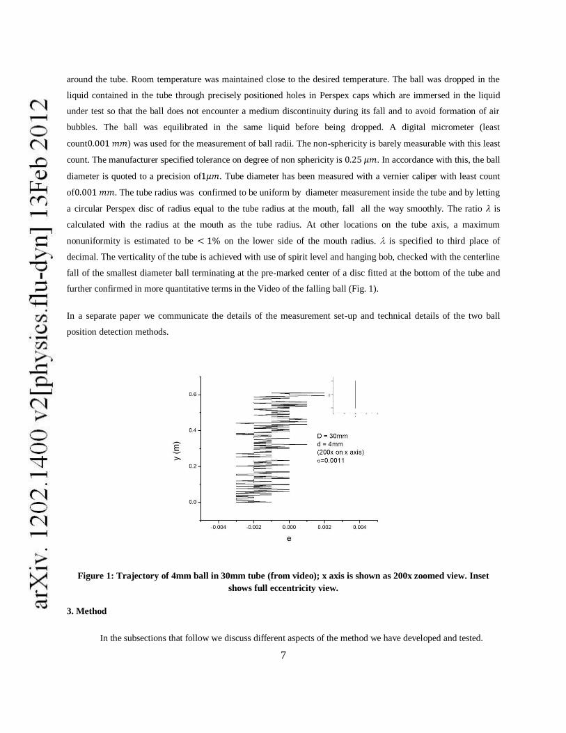
further confirmed in more quantitative terms in the Video of the falling ball (Fig. 1).
In a separate paper we communicate the details of the measurement set-up and technical details of the two ball
position detection methods.
Figure 1: Trajectory of 4mm ball in 30mm tube (from video); x axis is shown as 200x zoomed view. Inset
shows full eccentricity view.
3. Method
In the subsections that follow we discuss different aspects of the method we have developed and tested.

8
3.1. Relations between ratios
3.1.1 and : The definition of (Eq.3) written in an equation structure is
(7)
where is measured in a narrow tube. This definition and Eq. 6 gives (Sutterby [38])
(8)
an equality that holds at all and .
3.1.2 and : As already noted, for a given ball-fluid combination the sum of the force of gravity and
that of buoyancy must equal frictional force in condition of steady fall. The sum is independent of whether the
falling ball is in a narrow tube or in a boundless medium. One can then equate in a narrow tube (Eq. 7) to that in
a boundless medium (substitution of = in Eq. 6 obtains )
(9)
It follows:
(10)
This is the desired relation. We recognize L.H.S. of Eq. 10 as (by Eq. 8) and conclude that the ratio of
and is , a relation we refer to in sec. 1.6.
We use abbreviations
(11)
Then Eq. 10 becomes
(12)
Experimental information is available on the two factors that appear on the RHS of Eq. 10. The data have
been parameterized (section 3.2) in terms of , a geometric parameter pertaining to the ball and the tube and ,

9
which is specific to a ball-liquid pair. It is therefore, possible to calculate (Eq. 10) over the whole range of
and a wide range of . Using one calculates only . We give below the method of calculating from .
3.1.3 , and : Eqs. 2, 4, 5 and Eqs. 11, 12 give
= = (13)
(14)
, only can be calculated ; and are obtained from , with Eq. 13 and 14 if functional
dependence of and on (or ) and are known. The relation between and (Eq. 2 and 4) is given
in Eq. 15;
(15)
With a known and , substitution of the functional forms of and in Eq. 13, reduces it to
an equation in a single unknown . Similarly substitution of the functional form of in Eq. 14 reduces it
to an equation in a single unknown .
In order to solve Eq.13, we recast the equation in the following form:
(13a)
The values of at the intersection points of the plots of the two functions of , given in RHS and LHS, of
Eq. 13a, are roots of Eq. 13. Points of intersection of RHS and LHS of Eq.14 are roots of Eq. 14. are
evaluated at the values of at the point(s) of intersection (and ). We refer to these methods as ‗graphical-
methods‘. The number of roots in both cases depend on the functional form of the expressions, determined by those
of , in Eq. 13 and in Eq. 14. We give these functional forms in section 3.2 and
consider the issue of number of roots in section 3.4.5.
For a given ball liquid pair, characterised by a R.H.S. of Eq. 13a is independent. The ratio on the
LHS is tube diameter independent although the numerator and denominator are not. In the limit ( ) and
equals , the Stokes Reynolds number.
10
3.2 Correlation formulae:
3.2.1 and : Clift equation and Cheng equation:
Clift et. al. [1] in a thorough summary of experimental results performed by different workers over many
years recommend formulae for over a wide range of Reynolds number with excellent predictive
accuracy. Functional form of the formulae depend on range. Subsequent research on the design of these
formulae (Turton and Levenspiel [48], Brown and Lawler [49], Cheng [40]) focus on simplification of their
structure to achieve range independence and incorporate small improvements in their predictive accuracy. We have
used the equation of Cheng [40] given in Eq. 16, because of its range independent functional form ( x ).
The equation of Clift [1] valid in the range , is given in Eq. 17.
(16)
(17)
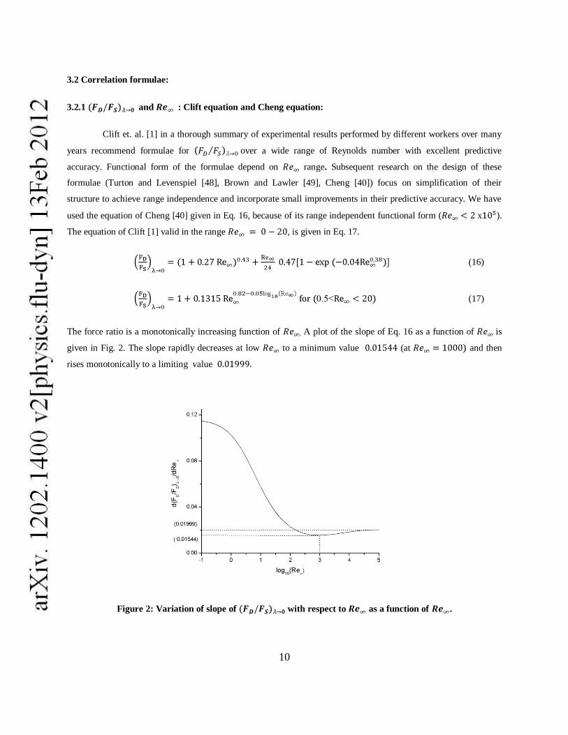
The force ratio is a monotonically increasing function of . A plot of the slope of Eq. 16 as a function of is
given in Fig. 2. The slope rapidly decreases at low to a minimum value (at and then
rises monotonically to a limiting value
Figure 2: Variation of slope of with respect to as a function of .

11
3.2.2 ( , ), DiFelice equation: DiFelice [33] proposed an equation for wall factor that accomodates
inertial effect with the aid of a single dependent parameter.
The equation is:
(18a)
where and , a function of that quantifies the inertial effect is defined as
(18b)
We observe that is 0.85 in the limit of very large and is at , i.e., it nearly saturates at
. This early saturation is not consistent with experimental results in the intermediate regime. This
deficiency was rectified in a subsequent paper of Kehlenbeck and DiFelice [34], henceforth referred to as K &D.
The equation, henceforth called K-D equation, gives satisfactory results over a very wide range (K & D,
Chhabra [32]). It forms an important component of this paper. This improvement necessitated introduction of a
second dependent parameter in K-D equation.
3.2.3 ( , ), K-D equation : The two parameter K-D equation is
(19a)
where and , are defined as follows:
(19b)
( ≤ 35) (19c)
=2.3 ( ≥ 35) (19d)
These formulae summarize experimental data on in the parameter range ,
. However, K &D have shown that their equation holds at as high as 10,000 and as low as with
nearly equal predictive accuracy. A detailed examination that we report later in the paper shows that the accuracy at
low is not as satisfactory as it is at higher Correlation formulae designed to predict
at a given have been proposed earlier (Chhabra [32]), but that by K &D is of special interest to our
work because it correlates over nearly whole range. These authors determined in the intermediate

12
range in which available experimental data were scanty. Their parametrization of in this range is the only
available formula of high predictive accuracy.
In contrast to DiFelice equation, K-D equation saturates at a much larger , viz. 105 ( as
, at = 100, at = ). This feature makes K-D equation successful in the intermediate
range, where changes systematically, though slowly. The experimental data at different values of and
their agreement with the predictions of K-D equation are given in KD. In Fig. 3, we show plots of , a
decreasing function, at different fixed values of as given by K-D equation. The slow saturation is apparent. It is
an increasing function of , which saturates at large for a fixed (Fig. 4 of F&W). The plots
in the intermediate range of are S-shaped. At large the shape is hyperbolic.
Figure 3: Functional dependence of on as given by K-D equation for a wide range of .
3.2.4 ( , ): Wham Equation: Wham et. al. [41] use finite element method for simulation studies on a falling
ball in a liquid medium contained in an infinitely long narrow tube ( , ) open at both ends
(no end effect), to obtain dependence of ( = ), Eq. 8 and 11) on and . The governing equations are
Navier-Stokes equation and the continuity equation. Their data is represented by Eq. 20 and henceforth is referred to
as Wham equation.
(20a)
where, ) (20b)

13
The corresponding expression in Wham et. al. [41] uses a definition of Re , where r is ball radius) that
differs from the usual definition, we give in Eq. 4. In Eq. 20 we use as defined in Eq. 4. L.H.S. of Eq. 20a is
. By Eq. 12 equals the ratio of Eq. 16 and 20a.
3.3 The Limiting forms:
3.3.1 Cheng Equations: In the limit R.H.S. of Eq. 16 approaches unity. In the limit of very large
(~ its approximate form is: 0.5 .
3.3.2 Wham Equation: The limit of Wham equation (Eq. 20) is
(21)
The H-S equation is
(22)
No assumption is implicit in obtaining this limit . Eq. 21 has an identical structure and nearly equal
coefficient values (the coefficient linear in is slightly different, instead of in Eq. 21) as the H-S
equation (Eq. 22). Its range of validity is and . The limit is the same as the limit .
The function used in fitting simulation results in the work of Wham et. al. [41] appears to have been chosen in such
a way that in the limit it ‗nearly‘ reduces to H-S equation.
An expression for can be derived from Wham equation if we (incorrectly) assume that Eq. 20
holds in the limit Then the second bracketed term of Eq. 20a is unity and in the first term is replaced by
This equation gives values that differ considerably from those given by Eq. 16 to show that Eq. 20a in the limit
is not valid.
3.3.3 DiFelice equation and K.D. equation: In the limit DiFelice equation assumes a limiting form with
= 3.3 (Eq. 18a). K-D equation assumes a limiting form with (Eq. 19b), = 1.44 (Eq. 19c). In this
limit equals .
3.3.4 and at large : With increase in , is progressively insensitive to increase in (Fig. 4 of
F&W and Fig. 1 of DiFelice [33]). independence of ( at large has been noted (Clift [1], Munroe
[50], Arsenijevic [51]) and has a functional form different from that in the limit. The large limit is

14
dependent ( of at , at ). Although is insensitive, is not, since
increases with . Wham equation is not valid beyond . Wham‘s equation of remains
dependent upto its upper limit of validity, .
3.3.5 Stokes limit: We deduce some features of approach to Stokes limit with the aid of equations cited above We
note (i) for , (Eq. 18), for any (ii) for (Eq. 16, 17), we use
Eq. 10 and shown in (i) to conclude, that for any and , , (iii) in the limit
, (Eq. 16, 17), as a result = for all ; an equality referred to earlier
(iv) is a sufficient condition for 1 (Eq. 18); is not necessary (v) combining (iii) and (iv)
we conclude that only if conditions for validity of Stokes equation, and hold
simultaneously (vi) Stokes limit , therefore is not implied by , must also hold.
3.4 Calculation Schemes: In this section, we detail procedures of calculation that are used in later developments.
The same quantity is calculated by several different procedures and their accuracy is assessed.
3.4.1 , , , : Cheng equation and K-D (or Wham) equation: We use a known value of to
calculate as outlined below. We use (i) Eq. 16 (ii) the knowledge that in state of steady fall equals the sum
of the forces of gravity and buoyancy (iii) Eq. 6 with substitution of in place of to obtain and (iv) Eq.
2 which defines in terms of . We then obtain an equation in a single unknown variable , which is solved
iteratively to obtain numerical value of (and then from Eq. 2). This calculation requires as input the
accurately known values of physical parameters of the ball-liquid pairs, namely and Using this value of
(designated ) and that of we calculate by Eq. 19. Use of the value of , Eq. 16, Eq. 12 and the
value of gives . These values are designated , respectively, to distinguish them from their
counterparts defined in sec. 3.4.2 and 3.4.3. One substitutes the value of in Eq. 2 to get (designated and
further Eq. 11 and the value of to calculate .
If Wham equation is being used, we must still use Cheng equation to calculate from . We then
solve Eq. 15 iteratively, as detailed below, to calculate numerical value of and (referred to as ) given the
value of . The functional form of is given by the product of RHS of Eq. 16 and Eq. 20a. The expression is
reduced to a function of a single variable by substitution of the numerical value of , as calculated from Eq.
16, and that of . is then calculated. Eq. 4 gives value of from that of . Value of and that of with Eq.
20 gives the value of .
3.4.2 , , , : K-D equation and Cheng Equation: We substitute the forms of Eq. 16 and Eq. 19 in
Eq. 13 which is restructured in Eq. 13a. is an experimentally determined input to this equation. The solutions
are , , . This combination of equations henceforth referred to as KDC equation, is solved most

15
transparently by a graphical method given in sec. 3.1.3 (also Fig. 4). One scans over the whole range ( ),
obtain the intersection points of the plots of RHS and LHS of Eq. 13a. With of each intersection point and
one calculates the respective and . With use of experimentally determined , one obtains for each .
Choice between the roots, if there is more than one, is based on additional information (sec. 3.4.5). In essence
knowledge of Eq. 16 and 19 enables us to calculate without performing a velocity measurement in infinite
medium.
Figure 4: Plot of as a function of ; three possible cases.
In an equivalent procedure we may adapt the method of calculation of from (sec. 3.4.1), in reverse to
calculate from . One (i) scans over a range; (ii) calculates for each ; then (iii) correct value of is
one that gives experimental value of . These two methods are convenient in search of multiple solutions of Eq. 13a
by KDC procedure. A standard iterative procedure can also be used to determine , and together in a
single step. and give by Eq. 11.
, , and determined from and K-D equation are designated , and
respectively.
3.4.3 , , , : Wham equation: We substitute in Eq. 14, the functional form of specified in Eq.
20 (Wham equation), solve it to calculate, for a given , the numerical value of and and thence . In
this procedure we do not calculate explicitly in the process of calculating .
16
In order to calculate values of and we use the route specified below. The values are
obtained together in a single step as solution of Eq. 15. The expression of we use, is product of RHS of Eq. 16
function of and that of Eq. 20, a function of ( , ). The expression is reduced to a function of a single
unknown by substitution of numerical values of as calculated above and . We obtain values of and
at a specific ( , ). This value of is determined for data and Wham equation and is designated as
(Wham).
3.4.4 : In sec. 3.4.1 we calculate given as an input. In sec. 3.4.3 we calculate given (or ) as
an input. They are designated and respectively.
3.4.5 Uniqueness of calculated parameters: We consider the graphical method of solution of Eq. 13, using
equation structure of Eq. 13a, as given in sec. 3.4.2. The roots of Eq. 13a are obtained from intersection points of
( ), and (RHS and LHS of Eq. 13a as functions of ).
The function , RHS of Eq. 13a, shown as a plot in Fig. 4 has a single maximum with a
function value for . The values fall monotonically on both sides of the maximum; to zero as
and to as assumes large values , the upper limit of validity of Eq. 16.
A plot of vs. is determined by the experimental value of , a fixed input and has the
shape of at a fixed as a function of . For given values of physical parameters of the ball-liquid pair
, and assumes larger values for liquids of low and is increasingly smaller as increases for a
given . The plot of vs. shifts upwards to larger values on y-axis with increase in and/or
increase in . Fidleris and Whitmore [36] give the shape of as a function of ( ) for several values of in
Fig. 3 of their paper. The plots are flat at small values of ( ) and decrease to show another flat region (which is
not as flat) at high values of ( ).The flat region at low ( ) extends up to larger values of ( ) as
decreases. The difference in the values of in the two flat regions increases with increasing . Thus, at smaller
vs. has a very flat appearance over the whole range. At a larger its decrease from one flat
region to the other and consequent saturation becomes increasingly more apparent. In this larger family the value
of at which saturation is observed increases with increasing . The shape of vs. ) will be
similar. In many scans the low flat region is omitted (being at first intersection) and one observes
an initial decrease followed by a somewhat flat region on plot (Fig. 4).
An examination of Fig. 4 shows that multiple solutions are obtained only for large values of (x-
coordinate) and (y-coordinate); for the first intersection
point. In this range of values scanning beyond the first point of intersection keeps plot a straight line
parallel to axis, followed by a second point of intersection at a larger value of . Beyond this second point

17
the plot of remains parallel to the asymptotic straight line plot of . As a consequence,
more than two alternate values of will never be obtained as solutions of Eq. 13a.
At the intersection point the equality specified by Eq.13a holds and is determined by
alone, i.e., by the ball-liquid pair and is independent of the tube diameter. One can however choose a value of
by identifying a suitable ball radius and density which for a given liquid will give an unique value or a pair of values
of as solution of Eq. 13a.
The two roots merge if at . The two plots touch each other at
and do not cross again. With even a small extent of error-contamination, already large values of
at a large may exceed at .The plot of in such a case remains above that of
for all values of .There exists no point of intersection and then Eq.13a has no solution
(Fig.4).
The two values of that correspond to the two intersection points, for a given give two different
values of . The feature of two roots arises only if the value of at the first point of intersection is large
( , as is the case with low viscosity liquids. is insensitive to for large values of . As a result
the two values of correspond to closely spaced . Irrespective of whether the two values of are closely
spaced or are significantly separated, the corresponding values of will be different because of significantly
unequal . The two calculated values of are then different. The larger value of obtained at the second
point of intersection will result in a smaller value of . In the cases we study and discuss in sec. 4.3, their values
are such that an unequivocal choice is possible. The separation in values between the two alternate and
corresponding decrease with increase in and . If the difference is small, the choice may not be so
unequivocal (Fig.4). Choice of a smaller ball diameter, and a smaller ball density (Teflon ball instead of Steel balls)
can take a system out of the multiple root regime into the unique root regime or from two closely spaced roots to
two separated roots. The ambiguities are then satisfactorily resolved.
3.4.6 , → : The estimates of , made in sec. 3.4.1, 3.4.2, 3.4.3 use as experimental input only
or only . One may use both and to calculate them. has been calculated as ratio of (determined
experimentally using independent viscometers) and , that uses (Sutterby [38]). is calculated as follows:
is calculated from already ‗known‘ and Eq. 16 (sec. 3.4.1). With Eq. 11 and experimental one obtains . The
ratios , so calculated are designated and respectively. The ( , ) pair are related by Eq.
12 and 16, with calculated as in sec. 3.4.1 from ‗known‘ values of .
3.4.7 Analysis of Error: In ‗Results and Discussions‘ we infer that the functional form of Eq. 16, 19, 20 used in
calculations may require modification of their form to remove inconsistencies in calculated values. Of these three,
Eq. 19 and 20 have a larger probability of having an inexact form than does Eq. 16 (sec. 4.3.1, 4.3.2). Scatter of
18
accurate experimental values are present around those given by the ‗best‘ of such functional forms. Inaccuracy so
introduced is inherent in the choice of a functional form. In sec. 4.3.1 and 4.3.2 we conclude that the functional form
of Eq. 16 be taken to be ‗exact‘ but Eq. 19 or 20 may be amenable to small modifications. The method used for the
analysis of this error transmission given in the following subsections, makes this assumption.
3.4.7.1 : The values of are not contaminated by errors in ‗inexact‘ functional forms of Eq. 19 and 20. In
addition to values of , , one uses only Eq. 16, which is a high accuracy representation of experimental data of
(sec. 4.3.1). One can say that they are obtained from accurate experimental data alone.
We define the error in as
(23a)
is further decomposed into two components as defined below
(23b)
(23c)
(23d)
Corresponding error terms in Wham calculations are defined identically. Of the three terms that appear in Eq.
23c and 23d, and derive error form an inexact functional form of Eq. 19. uses Eq. 19 with
calculated from Eq. 16 alone (Eq. 19 not used). used Eq. 19 with , whose calculation further uses
Eq. 19 (in Eq. 13a). As a result ( is less accurate) and the correct
value of can be thought of as having been obtained by substitution of
in the correct functional form of (which may not be known) and uses the same in the incorrect
form given in Eq.19. is an estimate of what may be called a purely form error.
3.4.7.2 : In view of excellent accuracy of the functional form of Cheng formula (Eq. 16) for (sec.
4.3.1) error in ( ) is derived almost entirely for that of the functional form of ( . Translation of to
is executed in two parts. For K-D equation this is denoted as: ,
. The transformations are dependent on the values of different estimates of . The relevent expressions
are given below
(24a)

19
(24b)
An inexact form of (Eq. 19) results in As a consequence the value of and that of
change. These changes combine according to Eq. 24(b) to give (KDC)
(24c)
We recognize the equality
(24d)
Eq. 24c then gives
(24e)
Eq. 24d and 24e give
(24f)
The ratio ( ) is always and becomes smaller as increases
The expression of (Eq. 24b) can be rewritten as
(25)
where, ;
is small in numerical value, more so at a large . The inequality
holds for small , particularly at a smaller . One then obtains
i.e., is necessarily small and can have either
relative sign. At a larger , increases in magnitude remaining below unity and

20
. Irrespective of the sign of . One then obtains a relative amplification of
with respect to ; there is a change of relative sign if it is positive and no change, otherwise.
A certain value of in two different regimes (viz., as against ) can result into values of
of different orders. We observe these features in our analysis of data in lower regimes in studies of Glycerol
and Silicone Oil and that in larger regime in study of Water. The magnitude of determines accuracy of
determination. The above considerations made with KDC equation have their counterparts in calculations with
Wham equation.
4. Results and Discussions
4.1 Dependence of on system parameters: Although, the relationship between and is known to high
accuracy in the limit 0 and to a lesser accuracy level at finite , it may not be possible to perform
experiments in this limit with an arbitrary liquid. There are restrictions on ball diameter imposed by difficulty of ball
detection in a given technique and on density of ball material which must exceed liquid density. For a given liquid
( and ) can be written as a function of and using Eq. 9 as follows:
(26)
Given the physical parameters of the ball and the test liquid one can use Eq. 26 and Eq.16 to compute from the
physical parameters of ball and liquid,. One finds that increases with , (for a fixed ), (for a fixed )
and decreases with ( Figs. 5a, 5b).The increase of with increasing is more rapid than quadratic. is
an increasing function of . We use this result in sec. 4.2.2.
In Fig. 5a we note that with small , and = (5 a virtual lower limit on grounds of
ability to detect the ball position and availability of suitable ball material, one obtains a which rises to
for in a low viscosity liquid like water. The value of is larger as for a given or for
a given is increased. These problems are less acute for more viscous liquids. We infer that one must validate
methods for calculation of by falling ball viscometry at values of well beyond the 'creepy flow‘ regime, an
exercise we have undertaken in this paper.

21
Figure 5a: vs. ,difference in density between
ball and liquid
Figure 5b: vs. ,diameter of the falling ball
4.2 Our experiments at Lower Re∞:
4.2.1 Terminal velocity data: A combination of seven balls diameters and three tube diameters
are used in measurements of . The values of for different ball-tube combinations are given in
Table 1. In Table 2 we summarize experimental results on . Silicone oil and Glycerol at are the test liquids in
two experiment sets. With Silicone oil, we vary for a fixed and also for a fixed . With Glycerol, we carry
out only the first variation in the tube with the largest . Only five values of could be
used in experiments with Silicone oil in the narrowest tube . Reported experiments are performed
with steel balls. Five measurements are performed for each ball-tube pair. The range of in velocities in percent for
Silicone oil in 40mm tube is in tube is and in tube is
respectively. The errors are independent of . In measurements on Glycerol in 40mm tube the
range is . In the case of Glycerol the error increases with increasing and in all cases is larger than
that for Silicone oil, still remaining small compared to most literature reports. The difference may arise from the
more complex liquid structure of Glycerol. The typical values of for ball density and ball diameter are and
respectively. These errors contribute negligibly to random errors of , so does the uncertainty in liquid
density . The random error in estimating tube diameter is also of negligible consequence. The tube diameter
non-uniformity which may contribute to a systematic error has been estimated to be less than and does not
alter our conclusions. Some literature reports on repeatability of measurements are: K-D, (stop-watch);
Brizard [7], and less (CCD camera); Tran-Son-Tay et. al. [28], in viscosity (ultrasonic); Flude and Daborn
[52], , (and 0.3% in viscosity) (Laser Doppler). Our precision is comparable to the very best of the reported
22
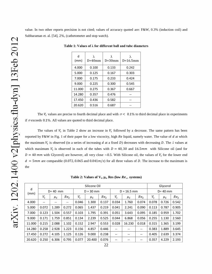
value. In two other reports precision is not cited; values of accuracy quoted are: F&W, 0.3% (induction coil) and
Subbaraman et. al. [54], , (cathetometer and stop watch).
Table 1: Values of λ for different ball and tube diameters
d (mm) D=40mm D=30mm D=16.5mm
4.000 0.100 0.133 0.242
5.000 0.125 0.167 0.303
7.000 0.175 0.233 0.424
9.000 0.225 0.300 0.545
11.000 0.275 0.367 0.667
14.280 0.357 0.476 --
17.450 0.436 0.582 --
20.620 0.516 0.687 --
The values are precise to fourth decimal place and with to third decimal place in experiments
if exceeds . All values are quoted to third decimal place.
The values of in Table 2 show an increase in followed by a decrease. The same pattern has been
reported by F&W in Fig. 1 of their paper for a low viscocity, high liquid, namely water. The value of at which
the maximum is observed (in a series of increasing at a fixed ) decreases with decreasing . The values at
which maximum is observed in each of the tubes with and with Silicone oil (and for
with Glycerol) are however, all very close . With Silicone oil, the values of for the lower end
are comparable ( and ) for all three values of . The increase to the maximum is
the
Table 2: Values of Vt, µs, Res (low systems)
d (mm)
Silicone Oil Glycerol
D= 40 mm D = 30 mm D = 16.5 mm D= 40 mm
4.000 -- -- -- 0.046 1.300 0.137 0.034 1.760 0.074 0.078 0.726 0.542
5.000 0.072 1.289 0.272 0.065 1.437 0.219 0.041 2.241 0.090 0.113 0.787 0.905
7.000 0.123 1.504 0.557 0.103 1.795 0.391 0.051 3.643 0.095 0.185 0.959 1.702
9.000 0.171 1.759 0.851 0.134 2.239 0.525 0.044 6.868 0.056 0.255 1.130 2.560
11.000 0.215 2.088 1.102 0.152 2.947 0.553 0.028 16.230 0.018 0.315 1.365 3.199
14.280 0.258 2.928 1.223 0.156 4.857 0.446 -- -- -- 0.383 1.889 3.645
17.450 0.272 4.105 1.125 0.126 9.000 0.238 -- -- -- 0.405 2.639 3.374
20.620 0.250 6.306 0.795 0.077 20.400 0.076 -- -- -- 0.357 4.229 2.193

23
least in the narrowest tube, a maximum of is reached at , in comparison to a much larger
maximum value of ( ) attained at a larger value of ( ) for tubes of larger
( ) respectively. The low values of attained for the largest value of in tubes of different
( in and for ) differ from each other more significantly
( ) than their counterparts at the lower end . The values at the larger end differ more
significantly than those in the lower end . With a given , as increases the value of shows a decrease for
Silicone oil.The less viscous Glycerol shows a larger for a given and .
4.2.2 On trends in terminal velocity data: In the following we interpret the trends terminal velocity data given in
section 4.2.1 in terms of Eq. 19 and Eq. 16. We use the following relation which follows from the definition of
(27)
(a) Fixed , varying : In an experiment set on with increasing at a fixed down a column of values in
Table , both and increase. It is known from experiments (F&W, K&D) and simulations (Wham [41]) that
decreases with increasing for a fixed (Fig. 3). With increasing Re and increasing variation of is not
monotonic, and work in opposition. However, of the two, dominates and in the limited range that we have
covered in a group of experiments with varying at a fixed , shows a decrease as increases in this set.
We use the result that is proportional to (Eq. 3) and that is an increasing function of
(section 4.2.1) to infer that is an increasing function of . We put the dependence of and on together
and Eq. 27 to infer that will show a maximum at an intermediate value of , as noted in sec.4.2.1.
(b) Fixed , varying : In this set, changes but not implying a constant (Eq. 3). With decreasing D and
and a constant Re∞ the value of decreases (subsection (a) above).We infer ( Eq. 27) decreases with increasing
for a fixed ,as noted in 4.2.1.
(c) Fixed , varying and : In this set changes but not . We note that increases with increasing
(section 4.1.1). At a fixed ,an increasing implies an increasing . We have noted that is also an
increasing function of . It follows from Eq. 27 that increases with increasing at a fixed System pairs in
Table 2 that illustrate this feature are; : ( ) and ( ); and
and .
4.2.3 Accuracy of terminal velocity data: The accurate measurement of coordinates and time, performed in the
video camera, imparts high accuracy to the values of terminal velocity we report. A possible source of significant
systematic error has however been identified in the literature. An off-axis movement of a ball falling vertically along
the centerline has been considered a possibility, at very low ( , on the basis of theoretical

24
arguments and some experimental reports (Ambari et. al. [17], [47]; Christopherson and Dawson [55], Bungay and
Brenner [56]). At a larger , a dependent horizontal force (Shinohara and Hasimoto [16]) operates to restore
any deviation away from an axial fall back to centerline. Off-axis movement at a very low is a consequence of
lower frictional force along a vertical axis away from the tube axis and the principle of minimum dissipation. This
principle requires that the ball falls along the line of minimum vertical frictional force. Ambari et. al. [17] have
shown by use of a magnetic rheometer that the eccentricity dependence of the frictional force that impedes the
vertical fall shows a minimum at an intermediate eccentricity, whose location shifts to larger values, as increases
(from to ). Experimental evidence for this very low off-axis fall has been reported for very large , when
the ball nearly fills the tube (Bungay and Brenner [55]).As the radius ratio approaches unity, the force ratio should
tend to infinity because of increased shear stresses between surfaces in relative motion. An additional effect arising
from ‗back flow‘ operates; as the sphere moves downwards, an equivalent amount of fluid moves upwards in the
restricted annulus between the sphere and the cylinder (Ambari et.al.[45]). Presumably with decreasing , these
effects decrease, but may not disappear. Error contamination of measured value of arising from an undetected off-
axis movement will make it larger than what it would be for a perfectly axial fall, causing to be smaller than its
actual value. This line of argument has been used to account for a larger measured in falling ball experiments of
F&W and McNowan [37] than that in magnetic rheometric measurements (Ambari et. al. [17], [47]). The latter
agree with ‗exact theory‘, but the former do not [47].
In our experiments the smallest Reynolds number, is , and the largest radius ratio is ; both lie
outside the range Bungay and Brenner [55] cite in their paper ( on experimental
reports on off-axis movement of a falling ball. Ambari et. al. [47] ‗suspect‘ such an off-center fall at smaller
but in their report (10 3) is still much smaller than in our experiment. Deviation from axial fall is
therefore not anticipated and is also not observed in our experiments in the videos we record. In the early falling ball
experiments of e.g. F&W the ball detection method was not capable of detecting off-center movements and could
have gone undetected. This is not so in the video detection of falling ball trajectory that we use. We conclude that
the terminal velocity values reported in Table 2 are free from any error due to possible off-center movement of the
falling ball.
The videos of a falling ball in our experiments show tiny fluctuations around the vertical centerline. These
off-center movements are not the ones Ambari et.al. [17], [47] refer to. We estimate error due to these off-centre
fluctuations in the next section and find them to be of negligible significance.
4.2.4 Verticality and off-center movements: We have estimated the error in due to off-axis fluctuations of the
falling ball trajectory as shown in Fig. 1 as follows. We calculate RMS deviation in position of the falling ball from
the center line. We assume that the ball trajectory deviates off-center all the way at an eccentricity ( ) specified by
the of horizontal deviation. We equate the frictional force for a centerline fall to that of an eccentric fall with
25
eccentricity . Both frictional forces equal , the sum of the forces of gravity and buoyancy. The formulae for
frictional forces in eccentric location of the ball are given by Tozeren [14]. For quiescent fluid and non rotating
sphere and of Tozeren‘s Eq. 5.1 are zero. The equation reduces to
(28a)
(28b)
Our is Tozeren‘s ; we also drop the superscript on . We designate centerline as VtC and off center as
. For will become . We define , recognize
as , as and obtain
(29)
The values of and are given in Tozeren [14]. The values of for and are
0.0011, 0.0014 and 0.0023 respectively and the corresponding values for are -2.42E-07, -1.74E-06 and
-1.84E-05 respectively. The deviations are within error of measurement of .
4.2.5 and : values and trends :We report in Table 2 values of , calculated from those of using Eq. 3,
and those of , calculated from those of and by Eq.5.In the following we interpret trends in these values.
We infer from a restructured Eq. 13a
(30)
that is a function of both the ball diameter ( ) and the tube diameter ( ) for a given liquid. On the RHS, a
function of and , the second factor in bracket is a function of alone and is a function of .
The dependence of on and can be related to that of by noting that is proportional to .
(a) fixed, changes: goes through a maximum with increasing , so does and ReS
(b) fixed, changes: For a fixed the pattern follows that of , a monotonic decrease at a fixed as
decreases.
(c) At a nearly equal (at two different , pairs) we assess the variation of with (and ) as follows: (i)
monotonically increases with increasing for , (ii) is a monotonically
increasing function of , (iii) therefore, monotonically increases with increasing for
26
, (iv) is a monotonically increasing function of and therefore of (v) as a result monotonically
increases with in the low regime for equal value of . Values in Table 2 confirm these conclusions.
is proportional to for a given liquid and density of ball material. As is decreased for a given ,
monotonically decreases and we observe a monotonic increase in . An increase in values of for a given
causes a monotonic increase in overshadowing the non- monotonic variation of , observed with increasing .
Relative errors in and are of the same order as that in .
Values of forms primary data set; and atre quantities calculated with alone. In the following
we discuss values of quantities, calculated with further use of Eq. 16 and Eq. 19.
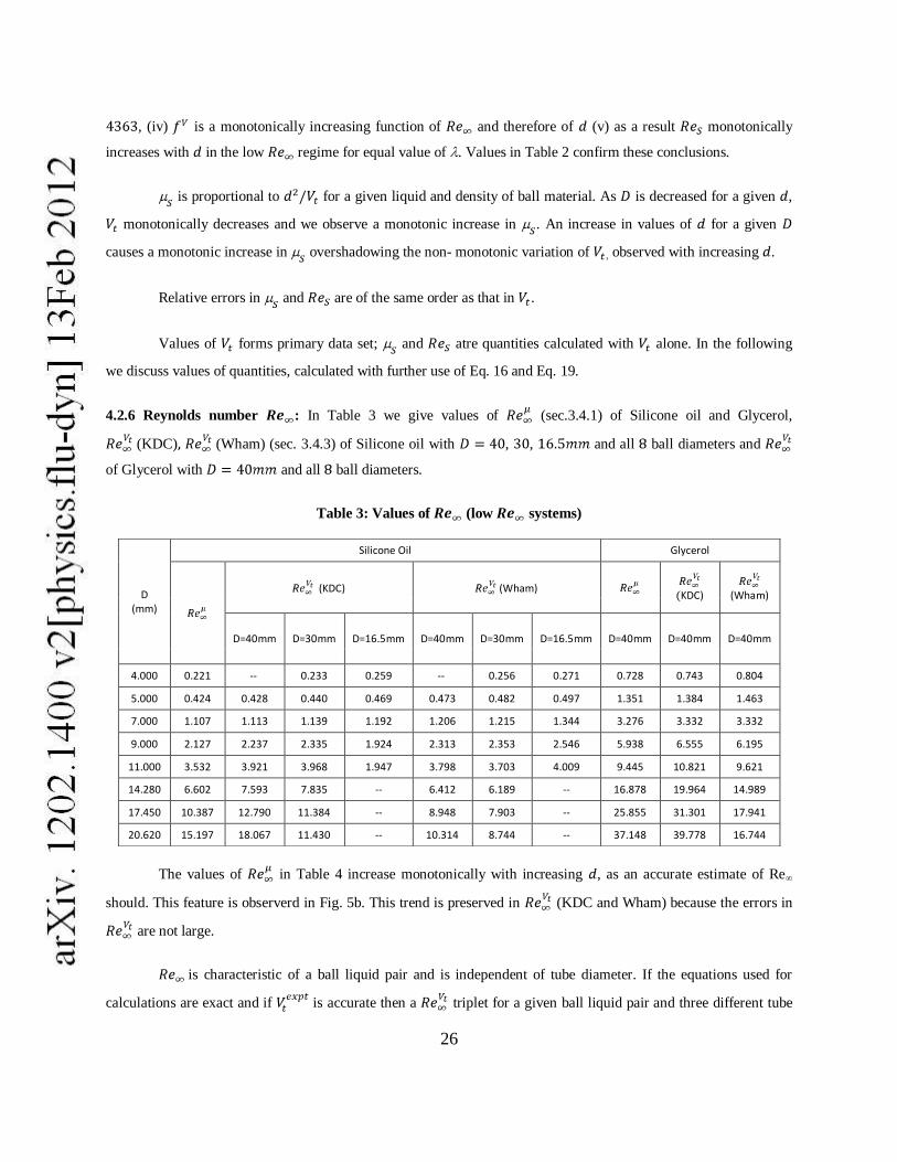
4.2.6 Reynolds number : In Table 3 we give values of (sec.3.4.1) of Silicone oil and Glycerol,
(KDC) (Wham) (sec. 3.4.3) of Silicone oil with , , and all ball diameters and
of Glycerol with and all ball diameters.
Table 3: Values of (low systems)
The values of in Table 4 increase monotonically with increasing , as an accurate estimate of Re∞
should. This feature is observerd in Fig. 5b. This trend is preserved in (KDC and Wham) because the errors in
are not large.
is characteristic of a ball liquid pair and is independent of tube diameter. If the equations used for
calculations are exact and if is accurate then a triplet for a given ball liquid pair and three different tube
D (mm)
Silicone Oil Glycerol
(KDC) (Wham)
KDC)
(Wham)
D=40mm D=30mm D=16.5mm D=40mm D=30mm D=16.5mm D=40mm D=40mm D=40mm
4.000 0.221 -- 0.233 0.259 -- 0.256 0.271 0.728 0.743 0.804
5.000 0.424 0.428 0.440 0.469 0.473 0.482 0.497 1.351 1.384 1.463
7.000 1.107 1.113 1.139 1.192 1.206 1.215 1.344 3.276 3.332 3.332
9.000 2.127 2.237 2.335 1.924 2.313 2.353 2.546 5.938 6.555 6.195
11.000 3.532 3.921 3.968 1.947 3.798 3.703 4.009 9.445 10.821 9.621
14.280 6.602 7.593 7.835 -- 6.412 6.189 -- 16.878 19.964 14.989
17.450 10.387 12.790 11.384 -- 8.948 7.903 -- 25.855 31.301 17.941
20.620 15.197 18.067 11.430 -- 10.314 8.744 -- 37.148 39.778 16.744

27
diameters should have equal values, equal to . Data in Table 3 show that (i) triplets, , ,
for all eight ball diameters for the same equation, KDC or Wham are unequal, i.e., tube diameter dependent, within
KDC set and Wham set separately; (ii) the two sets are not equal to each other; (iii) neither set is equal to .
Clearly an error is indicated. In view of the high accuracy of the values of (sec.4.2.3), we conclude that it is
necessary to assume that the functional forms of the equations used, e.g., Eq. 16, 19, 20 may have some
inexactness. An inexact form of ( , ) and alters the functions and
and changes the point of intersection in the graphical method of determination of (sec. 3.4.2, Fig. 4). In sec. 4.4,
we introduce small modification in Eq. 19 to remove these anomalies.
4.2.7 Bulk viscosity coefficient : Values of of Silicone oil and Glycerol calculated from those of by use of
KDC and Wham equations (designated and respectively) are given in Table 4. The most noticeable feature
of these data sets is that , a liquid specific ball-tube independent system property appears to vary with and .
An error is indicated.
Table 4: Values of (low systems)
d (mm)
Silicone Oil Glycerol
(KDC) (DC) (WC) (KDC)
(DC) (WC)
D=40 D=30 D=16.5 D=40 D=30 D=16.5 D=40 D=30 D=16.5 D=40 D=40 D=40
4.000 -- 0.983 0.932 -- 0.914 0.910 -- 0.935 0.907 0.598 0.527 0.571
5.000 1.004 0.989 0.956 0.910 0.909 0.939 0.952 0.942 0.927 0.594 0.505 0.576
7.000 1.005 0.992 0.968 0.877 0.896 0.951 0.961 0.957 0.905 0.596 0.479 0.596
9.000 0.979 0.955 1.068 0.838 0.874 1.030 0.960 0.951 0.908 0.565 0.446 0.586
11.000 0.946 0.939 1.433 0.821 0.911 1.200 0.964 0.979 0.933 0.550 0.443 0.595
14.280 0.921 0.904 -- 0.878 1.030 -- 1.027 1.053 -- 0.536 0.473 0.653
17.450 0.877 0.956 -- 0.965 1.260 -- 1.112 1.216 -- 0.526 0.536 0.776
20.620 0.896 1.222 -- 1.160 1.500 -- 1.308 1.459 -- 0.573 0.729 1.051
Values of of Silicone oil show a monotonic decrease with increasing (as varies) in
till it reaches a minimum beyond which an increase is observed. of Glycerol in tube shows
essentially the same pattern. In with Silicone oil a small initial increase followed by a decrease to a
minimum at is observed. The minimum is followed by a rise at . The minima
in the two tubes appear at comparable values of . At the values where a minimum in is observed assumes a
maximum value. In , the minimum in disappears, a monotonic increase in with increasing
is observed. The disappearance of the minimum has its counterpart in a very small maximum in obtained in this
narrowest tube.
28
The pattern of dependence of of Silicone oil and Glycerol on and is different. In all three tubes
with Silicone oil an overall increase which is not monotonic is observed. The same pattern is observed in of
Glycerol with when is varied. The variation of with increasing at a fixed follows the same
pattern as except that the minima is shifted to a smaller value of .
The error indicated in the lack of constancy of does not arise from ; (i)if we assume that an off axis
movement of the falling ball makes , as is ‗suspected‘ at (Ambari et. al. [47]) we
have and ,inequalities that do not hold in all entries in Tables 3 and 4; (ii) we have
consicered and ruled out off-axis movement of the falling ball in our experiments (sec 4.2.3, 4.2.4). We conclude
that lack of constancy of and the inequality are entirely due to inexact functional form of KDC, DC
and Wham equations.
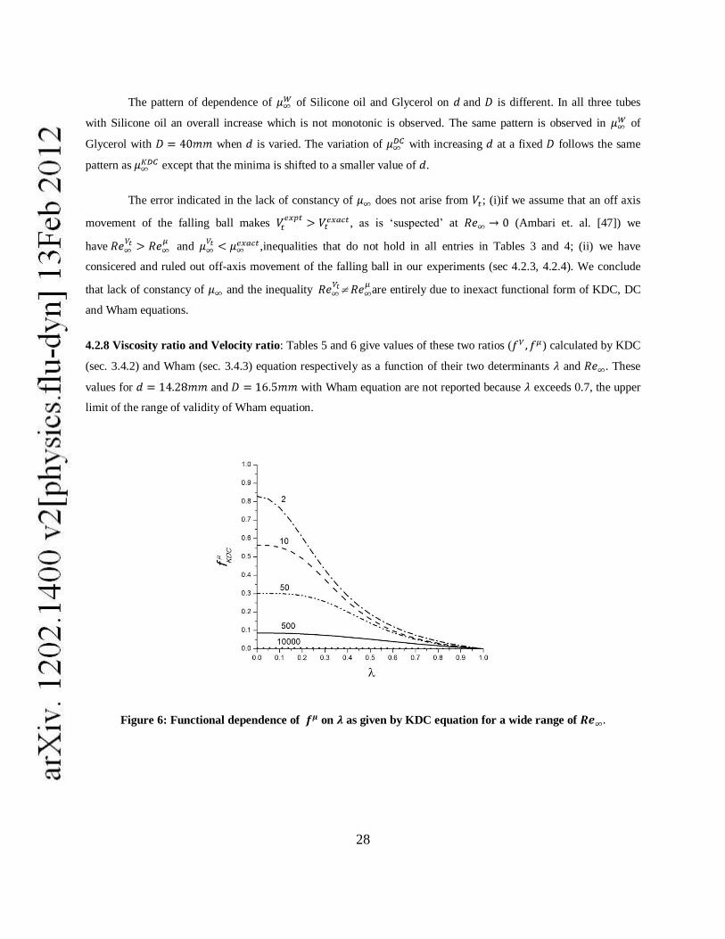
4.2.8 Viscosity ratio and Velocity ratio: Tables 5 and 6 give values of these two ratios ( ) calculated by KDC
(sec. 3.4.2) and Wham (sec. 3.4.3) equation respectively as a function of their two determinants and . These
values for and with Wham equation are not reported because exceeds 0.7, the upper
limit of the range of validity of Wham equation.
Figure 6: Functional dependence of on as given by KDC equation for a wide range of

29
Table 5: from values of alone (low systems)
d (mm)
Silicone Oil Glycerol
D=40mm D=30mm D=16.5mm D=40mm D=40mm
4.000 -- -- 0.778 0.758 0.543 0.528 0.889 0.822
5.000 0.817 0.780 0.724 0.690 0.450 0.428 0.875 0.775
7.000 0.749 0.669 0.622 0.554 0.300 0.266 0.827 0.638
9.000 0.684 0.557 0.528 0.427 0.187 0.156 0.809 0.541
11.000 0.621 0.453 0.438 0.319 0.106 0.089 0.768 0.448
14.280 0.512 0.315 0.306 0.186 -- -- 0.678 0.324
17.450 0.412 0.214 0.197 0.106 -- -- 0.572 0.234
20.620 0.310 0.142 0.111 0.060 -- -- 0.415 0.157
Dependence of and on and as given by KDC equation, are shown in Fig. 3 and 6 respectively.
In Fig. 3 we observe an increase in at a fixed with an increase in and a decrease in at a fixed with
increase in . The plots become increasingly insensitive to changes in as becomes large (100 upwads). The
dependence of is derived entirely from that of since is independent (Eq. 16 and 17). ( ) at
different fixed values of is shown in Fig. 6.
Table 6: from values of Vt alone (low systems)
d (mm)
Silicone Oil Glycerol
D=40mm D=30mm D=16.5mm D=40mm D=40mm
4.000 -- -- 0.744 0.723 0.532 0.516 0.858 0.788
5.000 0.779 0.739 0.693 0.657 0.438 0.415 0.846 0.732
7.000 0.723 0.640 0.604 0.534 0.285 0.249 0.822 0.622
9.000 0.674 0.546 0.526 0.425 0.166 0.132 0.797 0.519
11.000 0.628 0.462 0.450 0.333 0.079 0.058 0.763 0.436
14.280 0.544 0.351 0.333 0.217 -- -- 0.704 0.346
17.450 0.464 0.271 0.223 0.135 -- -- 0.640 0.294
20.620 0.372 0.208 0.122 0.072 -- -- 0.527 0.249
The values of become progressively smaller at all as increases. The increase in ( , ) at all
with increase in is more than offset by a independent (Eq. 16 and 17) that is greater than unity
and monotonically increases with . At larger , values of are less sensitive to as is apparent in the
progressively flatter appearance of the plots in Fig. 6. Increase in and increase in have opposing effects on
values of but not on values of . Over the range of and values that we have investigated a decrease in
for in no case annuals the effect of increasing .
30
The trends of values in Tables 5 and 6 are consistent with those of Fig. 3 and 6 referred to above. In Tables
5 and 6, down each column (fixed ) and both increase. The effect of dominates and shows a
monotonic decrease. At concordant values of and in tubes of different diameters values of and are
closely spaced. At the largest and the values of and are quite small (e.g. , ,
and ), implying significant corrections to . In our discussion on correction factors at much
larger we find yet smaller (viz., ). Increase of by three orders of magnitude at comparable
increases , and decreased .
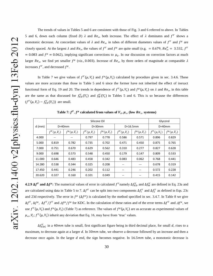
In Table 7 we give values of and calculated by procedure given in sec. 3.4.6. These
values are more accurate than those in Table 5 and 6 since the former have not inherited the effect of inexact
functional form of Eq. 19 and 20. The trends in dependence of and on and in this table
are the same as that discussed for and in Tables 5 and 6. This is so because the differences
( are small.
Table 7: calculated from values of , (low systems)
d (mm)
Silicone Oil Glycerol
D=40mm D=30mm D=16.5mm D=40mm
4.000 -- -- 0.797 0.778 0.586 0.571 0.896 0.829
5.000 0.819 0.782 0.735 0.702 0.471 0.450 0.875 0.765
7.000 0.751 0.670 0.629 0.562 0.310 0.277 0.827 0.628
9.000 0.698 0.573 0.548 0.450 0.179 0.147 0.809 0.533
11.000 0.646 0.483 0.458 0.342 0.083 0.062 0.768 0.441
14.280 0.538 0.344 0.325 0.208 -- --- 0.678 0.319
17.450 0.441 0.246 0.202 0.112 -- -- 0.572 0.228
20.620 0.327 0.160 0.101 0.049 -- -- 0.415 0.142
4.2.9 and : The numerical values of error in calculated namely and are defined in Eq. 23a and
are calculated using data in Table 5 to 7. can be split into two components and as defined in Eqs. 23c
and 23d respectively. The error in ( is calculated by the method specified in sec. 3.4.7. In Table 8 we give
, , and for KDC. In the calculation of these ratios and of the error terms and , we
use and (Table 7) as reference. The values of are as accurate as experimental values of
; inherit any deviation that Eq. 16, may have from ‗true‘ values.
in a tube is small, first significant figure being in third decimal place, for small , rises to a
maximum, to decrease again at a larger . In tube, we observe a decrease followed by an increase and then a
decrease once again. In the larger end, the sign becomes negative. In tube, a monotonic decrease is
31
observed, with a switch to negative sign beyond which its magnitude keeps increasing. values show a decrease
with increase in ( fixed), a changeover to a negative sign. The negative values show an increase in magnitude
with further increase in . In 16.5mm tube, the negative values are not observed. Mostly, K-D equation shows a
larger deviation from ‗correct‘ value of at intermediate values. In contrast, Wham equation shows a smaller
deviation at intermediate values, the deviation increases with different signs on two sides of this ‗intermediate‘
range. These complex features arise from effects of varying and .
in all but two entries(in both KDC and Wham) in Table 8 (the last two entries in Glycerol data) are
larger in magnitude than . in all cases, since (Eq. 11). As a result, in all
cases, even in the ones in which is < . In KDC calculations with Silicone oil the values of exceed 5% in
3/5 (D=16.5), 4/8 (D=30). 4/7 (D=40) entries and in those with Glycerol (D=40), in 4/8 entries, in Table 8. They
exceed 10% in 1/5 ( ), 2/8 ( ), 2/7 ( ) and in 2/8 (Glycerol, ) entries. All of these 7/28
entries with , have larger . In Wham calculations the errors are larger in 19/28 entries,
more significantly so at large and are smaller in the rest, which lie in the intermediate range, viz.
in , Glycerol; in , Slicone oil, where a switch over from positive
to negative error values is observed. Clearly large with accompanying large values increase error in
and increase relative error in .The accuracy of Wham equation at intermediate values is noted and is referred to
later.
Translation of proceeds as given in sec.3.4.7.2. In Table 9 we observe that both and
increase as one increases at a fixed and that is significantly larger. At a small
and can have either relative sign and are both small in value (sec.3.4.7.2).This is observed in Table 9. The
major contributor to is . equals in all cases, as it should be, by Eq. 24f.
The magnitude and sign of result from inexactness of functional form of correlation formula being
used and is expected to show no systematic variation with . Smaller value of (compared to ) results
from insensitivity of to change in (sec. 3.3.4, Fig.3). The sign of is opposite of that of in all cases.
is negative and small in all cases except three, in which it is positive and small. In these three cases
. As a result mostly, , remaining comparable and the pattern of variation of with (for a
fixed ) is the same as that of . Lack of systematic variation of with makes variation of
complex in Table 8.

32
Table 8: Error estimates in and in low systems
KDC
Wham
Silic
one
Oil
D=1
6.5m
m
0.242 0.044 0.076 0.042 0.072 0.055 0.097 0.054 0.092
0.303 0.022 0.050 0.021 0.045 0.035 0.078 0.033 0.071
0.424 0.011 0.038 0.010 0.031 0.028 0.100 0.025 0.081
0.545 -0.009 -0.062 -0.008 -0.046 0.014 0.098 0.013 0.070
0.667 -0.027 -0.427 -0.023 -0.281 0.004 0.071 0.004 0.045
Silic
one
Oil
D
=30m
m
0.133 0.019 0.025 0.019 0.024 0.055 0.071 0.053 0.067
0.167 0.012 0.017 0.012 0.016 0.045 0.064 0.043 0.058
0.233 0.008 0.015 0.007 0.012 0.028 0.049 0.025 0.040
0.300 0.023 0.052 0.021 0.038 0.025 0.056 0.022 0.041
0.367 0.023 0.068 0.020 0.044 0.010 0.028 0.008 0.018
0.476 0.021 0.102 0.019 0.057 -0.009 -0.045 -0.008 -0.025
0.582 0.006 0.051 0.005 0.025 -0.023 -0.208 -0.021 -0.104
0.687 -0.011 -0.213 -0.010 -0.099 -0.022 -0.449 -0.021 -0.202
Silic
one
Oil
D
=40m
m
0.100 -- -- -- -- -- -- -- --
0.125 0.002 0.003 0.002 0.003 0.043 0.055 0.041 0.050
0.175 0.002 0.002 0.001 0.002 0.031 0.045 0.028 0.037
0.225 0.016 0.028 0.014 0.020 0.027 0.047 0.024 0.034
0.275 0.030 0.061 0.026 0.040 0.021 0.043 0.018 0.028
0.357 0.030 0.086 0.026 0.048 -0.007 -0.019 -0.006 -0.011
0.436 0.032 0.130 0.029 0.066 -0.026 -0.104 -0.023 -0.052
0.516 0.018 0.111 0.017 0.053 -0.048 -0.298 -0.045 -0.136
Gly
cero
l D
=40m
m
0.100 0.008 0.009 0.007 0.008 0.042 0.050 0.039 0.043
0.125 0.010 0.013 0.009 0.010 0.033 0.043 0.029 0.034
0.175 0.006 0.010 0.005 0.006 0.006 0.010 0.005 0.006
0.225 0.032 0.061 0.028 0.035 0.014 0.026 0.012 0.015
0.275 0.038 0.086 0.034 0.045 0.005 0.012 0.005 0.006
0.357 0.035 0.109 0.034 0.051 -0.027 -0.085 -0.026 -0.039
0.436 0.029 0.126 0.031 0.055 -0.066 -0.289 -0.068 -0.118
0.516 0.007 0.047 0.008 0.019 -0.106 -0.746 -0.113 -0.271

33
is smaller in magnitude, with the same sign, than (Eq. 24). Also, , a result of a
similar inequality between the two components of . Unlike the ( , ) pair, the relation between and
is not monotonic, and do not always have same sign, but is comparatively reduced in magnitude
and contributes to a minor extent to .In no case has been amplified with respect to in the lower
regime under consideration and its sign has changed only in tube; its smaller magnitude makes the change of
sign unimportant. The opposite sign of and in all cases reduces to a level below , which is
primarily ( ).
Qualitatively one can understand the relative magnitude of and in the following terms: arises
from an incorrect value of , namely being substituted an incorrect functional form . arises
from a substitution of in an incorrect form and in a more accurate (Eq. 16). In this
case, use of introduces deviation in two places, which may act coherently or may mutually compensate. The
pattern of variation of is maintained in that of , as , which appears in the translation of to
(Eq. 29) varies over a limited range in the cases we study.
4.3 Correlation equations, graphs and tables : Accuracy issues:
The accuracy of the calculated values of , , and depend on the accuracy of functional forms of the
equations used viz., KD, Wham and Cheng equations.
4.3.1 : Cheng equation, Clift equation: Cheng [40] reports the average deviation of values of
predicted by his equation (Eq. 16) from experimental values as ~ 1.7% and a RMS deviation of 4.5%.The scatter of
carefully chosen experimental values around the prediction of its predecessor Clift equation (Eq. 17), which is very
close to it over the whole range is: 81.5% (±5%), 98.1% (±10%), 99.6% (±15%) (Brown and Lawler [49]). The
difference between average error and RMS deviation of Cheng equation from experiments suggests existence of
larger deviations in a small subset of the experimental data, as is also shown by the statistics of scatter data around
Clift equation. These formulae are based on a large number of carefully chosen experimental data published by
many different laboratories. The experiments being ‗accurate‘, the errors introduced by the choice of a specific
functional form are systematic. They are mostly ‗small‘ but can be significant in the small subset responsible for a
RMSD much larger than average error, e.g., 1.5% of values that deviate from Clift equation by >10% but <15% or
the 0.4% that lie beyond 15%. These errors are inherent in the use of best functional form. No ‗error‘ in the
functional form is referred to. We take the form of Eq. 16 as error free.

34
Table 8: Translation of and in KDC calculations in low cases.
Silic
one
Oil
D=1
6.5m
m
0.242 -0.007 0.000 -0.003 0.080
0.303 -0.006 -0.003 -0.002 0.051
0.424 -0.006 -0.007 0.002 0.037
0.545 0.008 0.018 -0.008 -0.054
0.667 0.043 0.103 -0.103 -0.324
Silic
one
Oil
D=3
0mm
0.133 -0.002 0.003 -0.001 0.026
0.167 -0.002 0.000 0.000 0.018
0.233 -0.003 -0.003 0.000 0.014
0.300 -0.011 -0.014 0.004 0.048
0.367 -0.017 -0.025 0.007 0.061
0.476 -0.029 -0.053 0.016 0.087
0.582 -0.015 -0.029 0.010 0.040
0.687 0.054 0.097 -0.061 -0.153
Silic
one
Oil
D=4
0mm
0.125 0.000 0.002 0.000 0.003
0.175 0.000 0.000 0.000 0.002
0.225 -0.005 -0.007 0.003 0.026
0.275 -0.014 -0.022 0.008 0.054
0.357 -0.026 -0.043 0.012 0.074
0.436 -0.047 -0.070 0.017 0.113
0.516 -0.045 -0.065 0.014 0.098
Gly
cero
l D
=40m
m
0.100 -0.001 -0.002 0.001 0.009
0.125 -0.001 -0.006 0.002 0.011
0.175 -0.002 -0.001 0.002 0.008
0.225 -0.013 -0.026 0.013 0.048
0.275 -0.023 -0.045 0.019 0.067
0.357 -0.040 -0.065 0.018 0.091
0.436 -0.059 -0.080 0.012 0.114
0.516 -0.023 -0.030 0.005 0.042
35
4.3.2 : Whereas formulae for (Eq.16,17)are functions of alone,those of is a function
of two independent variables, and . Number of data points, necessary for parameterizing a two-parameter
function with comparable accuracy level, is considerably larger than that for a single parameter function. Regarding
number of data points available for parameterization, the reverse is the case with and .
In what follows, we assess the accuracy of K-D equation (Eq. 19) in predicting experimental results. We
assess the accuracy of the experimental results on velocity ratio used for deriving this formula e.g., those of F&W
and those of K&D.
4.3.2.1 Fidleris and Whitmore [36]: These authors published an extensive experimental report on as a function
of and – . Their measurements have high accuracy ( Uncertainty in
values of is however significantly larger. The source of this additional uncertainty is that measurements could
not have been performed with their ball position sensing system, on the same ball-liquid combination on which
measurements were performed. The induction coil they use to sense the position of a magnetic ball falling along
center-line of a cylindrical tube would not register a signal if the tube diameter is very large limit). The
authors therefore use values of vs reported in the literature by other investigators who measured terminal
ball velocity in an infinite medium. These measurements were performed at values, for which values of
measured in a narrow tube were not available. In order to determine at a given and , the authors use a family
of continuous log vs plots (their is ) for different values of (including ) and a graphical
construction to evaluate . Experimental points are scattered around these smooth lines. Two sets of correction
factors, to calculate from ( / ) and vice versa ( / ), are reported. Their difference is an estimate of error
due to scatter around the smooth curves. The difference in the value pair is for , at
; is larger for as well as at ; (their Fig. 3 and 4). This uncertainty
decreases with decreasing for each .
Relative scarcity of experimental values of (narrow tube) at low and intermediate value of Reynolds
number in the work of F&W prompted experimental studies in these regimes (Sutterby [38], ,
Kehlenbeck and DiFelice [34], ).
4.3.2.2 Kehlenbeck and DiFelice [34]: The authors report in the intermediate range of ( ) by
determination of and for the same ball-liquid pair. Their method of terminal velocity determination use a stop
watch and can be used with equal facility in a narrow tube and in a large diameter tube. The uncertainty in their
values arises from the lower precision of their velocity measurements ( ) and not from the use of a correlation
graphs with its own inherent shortcoming, as is the case with values of F&W. Whereas F&W‘s errors are systematic,
K-D‘s errors are random.

36
The two parameter correlation formula of an assumed functional form has been optimized by K&D with
respect to their own data (all data points in their Fig. 2, and out of data points in Fig. 5,
are their own) and the data of F&W (5 out of 10 data points at are due to F&W, rest is from K&D). The
data of F&W that they use are obtained from the plots of F&W and are not primary experimental data. K&D do not
estimate the accuracy with which their equation predicts the mean values of / . We have estimated the deviation
of experimental data (mean values) that K&D used to deduce their equation, from the values calculated from K-
D equation. RRMSD of data points in Fig. 5 ( ) of K-D is , but it reduces to if values of
used in the estimate is restricted to . In Fig. 6 ( ) of K-D, RRMSD of about 10 data points is
. Both figures have one isolated instance of large relative deviation (viz. , ) which are so large
because they belong to data points with large i.e., small . An examination of their Fig. 8 which summarizes this
deviation without grouping them according to we find some large relative deviations in points with small . It
is a fair conclusion that, with a small ( ), the relative deviation is . The number of data points used
in this parameterization is considerably less than that used for deriving Clift or Cheng equation. K-D equation and
its predecessor DiFelice equation assume a specific functional form chosen on the basis of inspection of
experimental data using a fluid mechanical analogy. They find the best values of parameters of these equation forms
that fit the available experimental data or by using a fluid-mechanical analogy. The resulting formula is the ‗best‘
amongst a family and may not be best globally.
4.3.3 :
4.3.3.1 Wham et.al[41]: The authors estimate the predictive accuracy of the equation they derive (Eq. 20), i.e., the
extent of agreement between computational results on drag coefficients and the values calculated from their
correlation formula to be .. Satisfactory agreement with experiments is reported only at a specific value of
over a restricted range of ( ).
In view of the uncertainties discussed above, a small deviation in the correlation formula from its ‗exact‘
counterpart is only to be anticipated. An inherent systematic error (as distinct from random measurement error) is
introduced in fitting experimental data within a correlation formula. The uncertainty in fitting data is often larger
than random experimental error of measurement.
4.3.3.2 Sutterby [38]: The author reports 160 experimental values of and interpolates between these
points to work out a correlation table, for use with an unknown test liquid. Although a range was
studied, fewer data points were determined at larger (4 points above points above ) and
also at larger ( points ). Thus although very low and very low regime are adequately covered
by actual experimental points, one must rely on interpolated values as soon as and increases. The accuracy
with which Sutterby‘s tables predict his own ‗experimental values‘ is high, mean absolute deviation being , but

37
this agreement does not guarantee such a high accuracy level in those parts of , ) plot where actual
experimental points are scarce (Sutterby‘s Fig. 1, 2).The process of interpolation is not specified . The limit
for each is tied to a specific point by use of Faxen equation (Happel and Brenner [2b]. This limiting value
determines the curvature of the plot at low at each . The line corresponding to (the largest ) has
only 4 points, one each at and and two very closely spaced points at . A large part of this
line is experimentally unscanned and small errors may enter if a test liquid is examined in the unscanned region.
4.3.4 Limiting forms: The values of given by K-D and Wham equations in the limit , for
different values of are compared in Table 10 with theoretical estimates of (‗exact theory‘ and H-S
equation (Eq. 22)), with given in Eq. 21 (Wham equation). The limiting values determined by
theoretical methods fall in two classes: (a) ‗exact theory‘, as given in Haberman‘s thesis [42] that match nearly
exactly with results of several accurate calculations published later by Tozeren [14], Coutanceau [44] and Paine and
Sherr [43], summarized in Ambari et. al. [47] and (b) ‗approximate theory‘, namely H-S equation and the
limiting form of Wham equation (Eq. 21). Happel and Brenner (1983a) and Ambari et.al.[47] compare values of
obtained from ‗exact‘ theory and ‗approximate‘ theory and the difference increases with increasing .
The difference between different ‗exact‘ theories can be ignored in our context. The exact theory is in agreement
with the very careful experiments of Ambari et. al [47].
Table 9: Different estimates of
Values of Relative deviation from Exact-Threory
E-T* H-S K-D W D H-S K-D W D
0.1 0.792 0.792 0.787 0.790 0.789 0.000 0.006 0.002 0.003
0.2 0.595 0.595 0.648 0.592 0.600 0.000 -0.088 0.005 -0.008
0.3 0.422 0.422 0.452 0.417 0.435 0.000 -0.072 0.011 -0.031
0.4 0.278 0.279 0.329 0.273 0.296 -0.004 -0.184 0.019 -0.063
0.5 0.168 0.170 0.219 0.162 0.184 -0.017 -0.306 0.031 -0.099
0.6 0.090 0.094 0.142 0.084 0.101 -0.051 -0.582 0.061 -0.121
*E-T: Exact-Theory; W: Wham; D: DiFelice
The limit of Wham equation (Eq. 21) is, by design, almost identical in form to H-S equation(Eq.
22) and shows only slightly larger deviation from ‗exact‘ theory(Table 10). DiFelice equation (Eq. 18) has a
differently structured functional form; in the limit, however it gives values very close to those of Wham
equation (Table 10).
The values of show larger deviation from theoretical estimates in the range than
do the rest and are larger in value. In the design of functional forms of K-D equation and its predecessor DiFelice

38
equation, validity over an extended range and not in the limit is the prime focus. The inexact
limit of K-D equation, but a more exact limit of DiFelice equation results from a modification of equation
form to accommodate ‗intermediate‘ Re∞ range in K-D equation
4.3.5 Comparison of different estimates of over an extended range:
4.3.5.1 KDC and Sutterby: In Fig. 7a we compare values of as calculated by KDC equation and the values
given in Sutterby‘s tables (sec. 4.3.3.2). The difference at low is consistent with the deviation of from
given by exact theory, an indication of error in K-D equation in the limit of very small (sec 4..3.4). The
agreement at a higher indicates correctness of K-D equation in this range.
Figure 7a: Ratio of and Sutterby’s as a
function of for different values of specified in the
figure. The range of and are those of
Sutterby[38].
Figure 7b: Ratio of and those of Sutterby as a function
of for different values of specified in the figure. The
range of and are those of Sutterby [38].
4.3.5.2 Wham and Sutterby: In Fig. 7b we compare values of as given by simulation studies of Wham et.al[41]
with those given in the correlation tables of Sutterby[38], derived from experiments. The agreement deteriorates
with increasing value of ( ), for each . The deterioration is more rapid for which is outside the
range of validity of the relation given by Wham et.al [41] .The agreement is inferior at the lower end of
the validity range than at , which is well within the range. Sutterby‘s table does not go beyond
In the restricted range of where both correlations hold, Wham equation starts showing significant deviation from
Sutterby‘s results even at as low as 2.
4.3.5.3 KDC and Wham: Fig. 8 shows the plot of the ratio / , calculated using respective equations, at
several different values of as a function of . The agreement is good at low values of for .

39
Deviations from unity increase rapidly as increases at larger , but remains small (<10%) at smaller
over the in shown in Fig. 8.
At however, the ratio goes through a minimum, ~0.95 at and then monotonically
approaches to unity. The agreement between the predictions of the two equations, although ‗good‘ at and
, is best at (and around) over an extended range. At , is closest to , but
Figure 8: Plot of the ratio of and versus .
differs more significantly from (Table 4). In line with this is lowest(and smaller than ) at
around , where it switches sign, presumably going through zero. (Table 8). We infer Wham equation is more
correct than KDC equation around Wham et. al. [41] compare the predictions of their simulation results
with experimental results of McNown [37] at a value of very close to this value ( ) and report good
agreement in the range (Fig. 14 of Wham et. al. [41]). In sec. 4.5 when is modified to bring at
different values of as a set, closer to , the values of in the modified form are greater than those of
in its original form and come closer to at over an extended range.
The values of (Table 4) as a set, differ more significantly from than do the set . The
deviation increases more rapidly at a larger for . Deviation of from never becomes as large as
at large The same observations hold for the values of given in Table 3.

40
In Fig. 9 we compare values of calculated from the experimental data points determined by K-D and
reported in their paper (for details: sec. 4.3.2.2) and that calculated from Wham equation for two different values of
and . The larger value of at is consistent with the result that in this range K-D
Figure 9: Plot of the ratio of and versus . Values of are taken from Fig. 2 and 7 in K&D and
used in calculation of
equation gives larger values of as compared to the ‗exact theory‘ and Wham equation nearly reduces to H-S
equation, which is very close to ‗exact theory‘ (sec. 4.3.4, Table 10). The plot for shows agreement
better than 10% at 0.3, deteriorates significantly beyond and at all This is consistent with
Fig.8 and the larger values of as compared to for
We infer that KDC equation is overall superior to Wham equation in the range of
covered in experiments on Glycerol and Silicone oil.The values given by K-D equation at are slightly error-
contaminated, while those given by Wham equation in this Re range is more accurate than is KDC around
4.4 Test of the method at large : Data of Fidleris and Whitmore [36]:
4.4.1 data of Fidleris and Whitmore [36]: The method has been tested as described in sec. 4.2 in the smaller
range We now investigate its usefulness in a range of much larger ). Wham
equation is not valid beyond and therefore, we use only KDC equation. We use the experimental terminal
velocity data of 57 falls reported by F&W in their Fig. 1 for a wide range of values in tubes of four different
diameters on the test liquid water at 20 °C, a liquid having coefficient of viscosity ( ) about three orders

41
of magnitude smaller than that of Silicone oil or Glycerol. The values of in these measurements at large are a
factor of 5 or more, larger than in their low counterparts (Table 2). Accuracy of the measurements as
determined by F&W is 0.3%. Reading error increases this value marginally.
In Table 11 we give a subset of values given by F&W in their Fig. 1 for which, Eq. 13a could be solved.
These values show a non monotonic dependence on at a fixed (a non monotonic dependence), an increase of
with increasing , a maximum followed by a decrease. Numerical values (Table 11 and Fig.1 of F&W) are:
, a maximum in ( ) is observed with , ; ,
( ) with , ; , ( ) with , ;
, ( ) with , . The pattern in these data is a shift of for
to larger values as increases, remaining about the same. This pattern was observed with corresponding data at
low obtained with Glycerol and Silicone oil as test liquid, reported in sec. 4.2.1. The pattern of variation of
and , as varies for a fixed (Table 11) is the same as for Glycerol and Silicone oil (Table 2).
Table 10: Analysis of terminal velocity data of Fidleris and Whitmore for two tube diameter (20mm and
25mm) as a function of incerasing by use of KDC equation. of water at 20 is 0.00105 Pa.s (Fidlesris
and Whitmore (1961))
d
(mm) (m/s) (Pa.s) (Pa.s)
D =
20m
m
0.720 0.036 0.299 0.006 33.86 262.2 191.5 8.20E-04 2.19E-01
1.154 0.058 0.423 0.012 42.28 489.0 461.3 1.00E-03 4.76E-02
1.586 0.079 0.529 0.017 48.12 787.9 805.0 1.07E-03 -1.90E-02
2.020 0.101 0.621 0.024 52.06 1194.3 1206.8 1.06E-03
(-3.00E-05) -9.52E-03
2.400 0.120 0.689 0.031 53.94 1596.4 1596.4 1.05E-03
(-8.00E-05) 0.00E+00
2.820 0.141 0.764 0.038 56.44 3543.9 2062.0 6.20E-04
(-3.80E-04) 4.10E-01
D =
25m
m
0.600 0.024 0.303 0.004 41.73 466.5 134.2 3.90E-04 6.29E-01
1.173 0.047 0.426 0.012 42.21 480.1 474.7 1.04E-03 9.52E-03
1.565 0.063 0.524 0.017 47.84 754.0 786.9 1.09E-03 -3.81E-02
1.988 0.080 0.625 0.023 53.60 1341.5 1175.0 9.30E-04
(-4.00E-05) 1.14E-01
2.350 0.094 0.689 0.029 55.09 1698.3 1543.3 9.60E-04
(-9.00E-05) 8.57E-02
2.825 0.113 0.770 0.038 57.23 3141.9 2067.7 7.00E-04
(-3.30E-04) 3.33E-01

42
4.4.2 : The values of and are calculated by methods specified in sec. 3.4.1 and 3.4.2
respectively These values, along with those of , , and its relative deviation , in those cases where a
solution was obtained, are given in Table 11.The inequality noted in Table 3 (sec. 4.2.6) for low
systems is observed. The values of are larger, so are the differences between and , compared to those
in Table 3. > in all entries of Table 3. In contrast, in Table 11 the difference is not monotonic and changes
sign as increases. The values of and show trends observed in sec. 4.2.5 for low systems.
We also find in Table 11 that of water vary with change in This feature and the inequality
indicate an error. We assign, as we did for low viscosity results, an inexact functional form of the
correlation equations as the source of this error. In calculation of from , we obtain unique values only for very
low values of With increasing values of , a pair of values of are observed. It is apparent from Fig. 4 that the
two values come closer with increasing , as they do in Table 11. The values of in the largest entry for
both tube diameters in Table 11 approach the value at the maximum in Fig. 4. In this sequence, for yet larger values
of , no root was obtained in the whole range of scanned . One of the two values of , in systems that give a
root pair, is very close to the actual value. The other value is given in bracket in Table 11. being low, the accuracy
of the unique roots and the more ‗correct‘ root where a root pair is present, are excellent and deteriorates only
slightly in the largest entry of both tube diameters. In Fig. 11(a-d) we show values of , a single value or a pair
of values as the case may be, for all four tubes and discuss their accuracy in sec. 4.4.6.
Table 12: Values of calculated and 'exact' velocity and viscosity ratio for high
) )
D =
20m
m
0.036 1.054 0.999 0.158 0.129
0.058 0.999 0.997 0.087 0.087
0.079 0.985 0.994 0.058 0.062
0.101 0.986 0.990 0.042 0.044
0.120 0.981 0.985 0.033 0.034
0.141 0.991 0.979 0.026 0.016
D =
25
mm
0.024 1.270 1.000 0.231 0.090
0.047 0.993 0.998 0.085 0.088
0.063 0.985 0.997 0.059 0.064
0.080 1.002 0.994 0.044 0.040
0.094 0.995 0.991 0.034 0.033
0.113 0.999 0.987 0.027 0.018
4.4.3 and : In Table 12 we give values of , , , , for the falls analysed in Table 11
We note the following features in and of Table 12: (i) Pattern of variation of and with change in and
is the same as in low system (Table 5, 6). (ii)The values of at larger are larger(~1) as compared
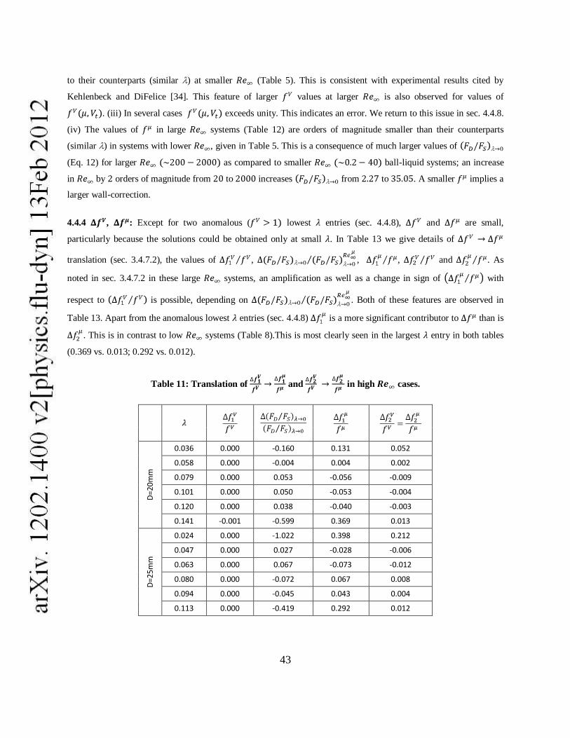
43
to their counterparts (similar ) at smaller (Table 5). This is consistent with experimental results cited by
Kehlenbeck and DiFelice [34]. This feature of larger values at larger is also observed for values of
. (iii) In several cases exceeds unity. This indicates an error. We return to this issue in sec. 4.4.8.
(iv) The values of in large systems (Table 12) are orders of magnitude smaller than their counterparts
(similar ) in systems with lower , given in Table 5. This is a consequence of much larger values of
(Eq. 12) for larger as compared to smaller ball-liquid systems; an increase
in by orders of magnitude from to increases from to . A smaller implies a
larger wall-correction.
4.4.4 , : Except for two anomalous ( lowest entries (sec. 4.4.8), and are small,
particularly because the solutions could be obtained only at small . In Table 13 we give details of
translation (sec. 3.4.7.2), the values of , , , and . As
noted in sec. 3.4.7.2 in these large systems, an amplification as well as a change in sign of with
respect to is possible, depending on . Both of these features are observed in
Table 13. Apart from the anomalous lowest entries (sec. 4.4.8) is a more significant contributor to than is
. This is in contrast to low systems (Table 8).This is most clearly seen in the largest entry in both tables
(0.369 vs. 0.013; 0.292 vs. 0.012).
Table 11: Translation of and in high cases.
D=2
0m
m
0.036 0.000 -0.160 0.131 0.052
0.058 0.000 -0.004 0.004 0.002
0.079 0.000 0.053 -0.056 -0.009
0.101 0.000 0.050 -0.053 -0.004
0.120 0.000 0.038 -0.040 -0.003
0.141 -0.001 -0.599 0.369 0.013
D=2
5mm
0.024 0.000 -1.022 0.398 0.212
0.047 0.000 0.027 -0.028 -0.006
0.063 0.000 0.067 -0.073 -0.012
0.080 0.000 -0.072 0.067 0.008
0.094 0.000 -0.045 0.043 0.004
0.113 0.000 -0.419 0.292 0.012
44
in larger cases is of comparable magnitude to its counterparts for smaller cases. This is to be
anticipated since these are purely form errors arising from defect in functional form alone (sec. 3.4.8.3) and may not
show any specific pattern in their dependence on . However, in the large systems is reduced to a
much smaller value as compared to its small counterparts (Eq. 24e; much larger ). The ratios
and are however equal (Table 13).
is smaller in water than their counterparts in smaller systems because of insensitivity of to change in
as grows larger. Even though the magnitude of ( ) is significantly larger for water as
compared to Glycerol and Silicone oil, the sensitivity of towards is so low at larger that in water
is negligibly small. is, however of the same order in water as compared to Glycerol/Silicone oil. (Table 9 and
13); As a result, the transformation of to is determined almost wholly by values of as given in
Eq. 25.
4.4.5 and : In large systems and are both orders of magnitude smaller for water as
compared to Glycerol/Silicone oil but may not have decreased by the same factor as does As a result
may assume larger values (Table 9 and 13), the largest in the set under study being (largest system
of set).
4.4.6 Calculated , Uniqueness and accuracy: In falls (all tube diameters), for of which is
small (below ), an unique value of (and ) could be calculated. These systems are easily identified in
Fig. 11(a-d): systems each in Fig. 11(a), 11(b) 11(c) and 11(d). The numerical value of for each solution is
given in the figures and for and also in Table 11. Five of these are accurate to , three are in
the range , three others have larger errors, namely (the lowest system in Fig.11(c)), and and
(the two lowest systems Fig. 11(d)). Values of (and ) for these unique solutions are smaller than those
of systems with multiple roots, as is expected (Fig. 4) The twelfth unique solution was obtained for ,
, a larger , accompanied by a smaller , compared to those for multiple root cases,
and for the three multiple root cases in order of increasing (non-monotonic variation of
with ). This result is consistent with Fig. 4. Calculated is , in error by ~ We have earlier
noted that the form of K-D equation is error-prone at large .
In falls for which is intermediate in a pair of values of
(and ) are found, 3 each in Fig. 11(a-d). Of these three systems in each figure the two with lower have one
root very close to the correct value of the other root is not so close. A larger deviation of both roots from the
‘correct root‘ is found for the largest system. In , the difference between the two solutions
decreases with increasing as is expected from Fig. 4. The choice between the two values is then ambiguous even
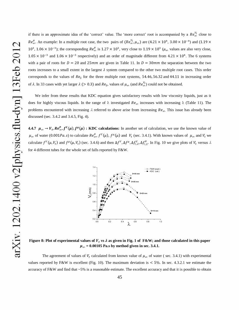
45
if there is an approximate idea of the ‗correct‘ value. The ‗more correct‘ root is accompanied by a close to
. An example: In a multiple root case, the two pairs of are ( , ) and (
); the corresponding is , very close to ( values are also very close,
and respectively) and an order of magnitude different from . The 6 systems
with a pair of roots for and are given in Table 11. In the separation between the two
roots increases to a small extent in the largest system compared to the other two multiple root cases. This order
corresponds to the values of for the three multiple root systems, and in increasing order
of . In 33 cases with yet larger and , values of (and ) could not be obtained.
We infer from these results that KDC equation gives satisfactory results with low viscosity liquids, just as it
does for highly viscous liquids. In the range of investigated increases with increasing (Table 11). The
problems encountered with increasing referred to above arise from increasing . This issue has already been
discussed (sec. 3.4.2 and 3.4.5, Fig. 4).
4.4.7 : KDC calculations: In another set of calculation, we use the known value of
of water ( ) to calculate , , and (sec. 3.4.1). With known values of and we
calculate and (sec. 3.4.6) and then . In Fig. 10 we give plots of versus
for 4 different tubes for the whole set of falls reported by F&W.
Figure 8: Plot of experimental values of vs as given in Fig. 1 of F&W; and those calculated in this paper
= 0.00105 Pa.s by method given in sec. 3.4.1.
The agreement of values of calculated from known value of of water ( sec. 3.4.1) with experimental
values reported by F&W is excellent (Fig. 10). The maximum deviation is . In sec. 4.3.2.1 we estimate the
accuracy of F&W and find that ~5% is a reasonable estimate. The excellent accuracy and that it is possible to obtain

46
values of in all cases is a result of a more accurate ,namely being available,as against in
calculations. This calculation assumes importance in view of the fact that in many applications the focus may be on
calculation of terminal velocity in a liquid of known viscosity coefficient in a given tube and not on determination of
viscosity coefficient of an unknown liquid.
4.4.8 In several ball-tube combinations we have obtained , an anomalous result. There are 3
such values in Table 12, viz., and . Similar anomalous systems have been observed in other tube
diameters, viz., , first 2 falls (lowest and ), ( and ; ,
first 4 falls, , , and An error is implied. Its calculation uses
the value of and Cheng equation (Eq. 16). Use of Clift equation marginally alters the values of and do not
remove the anomaly. The scatter of experimental values of drag ratio around those predicted by Clift equation (sec.
4.3.1) also contributes to this anomaly. Even after these errors are considered, is indeed an outlier. We note that
the four cases with large anomaly ( ) appear for systems with low
4.4.9 Anomalous : We have noted that over the whole range of , ( independent) assumes a
maximum value of at For a given , assumes a maximum value at a large . This
maximum value increases with decreasing (Fig. 3 and 4 of F&W). Consequently, has a
maximum value over the whole range of , for a given which increases with decreasing (Table 14). In Table
Table 12: Maximum possible value of for values given in Table 13.
(Max) (F&W)
0.036 58.96 33.86
0.058 58.75 42.28
0.079 58.42 48.12
0.101 57.92 52.06
0.120 57.36 53.94
0.141 56.60 56.44
0.157 55.92 58.25
0.180 54.79 58.00
0.196 53.89 59.52
0.238 51.14 53.57
0.318 44.52 47.27
0.397 36.73 39.32
0.472 28.93 30.05
0.635 13.62 14.58
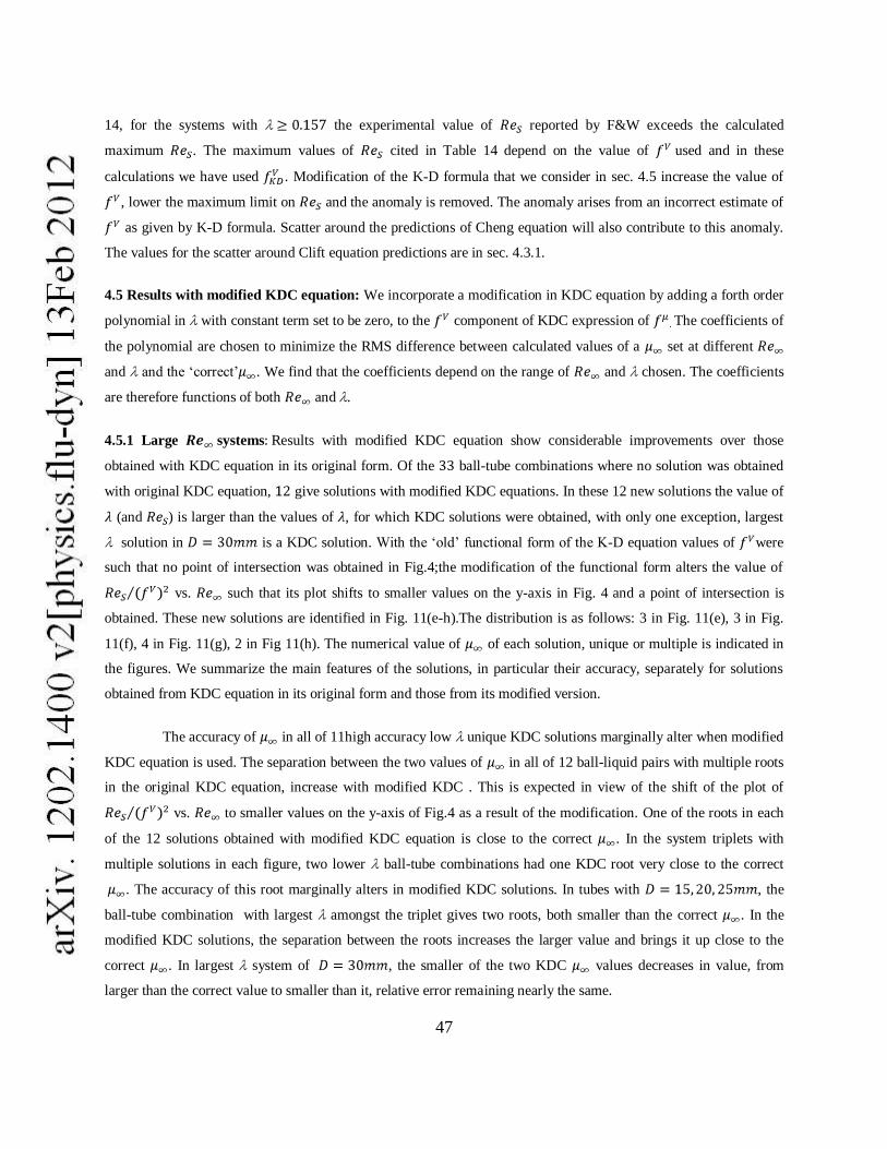
47
14, for the systems with the experimental value of reported by F&W exceeds the calculated
maximum . The maximum values of cited in Table 14 depend on the value of used and in these
calculations we have used . Modification of the K-D formula that we consider in sec. 4.5 increase the value of
, lower the maximum limit on and the anomaly is removed. The anomaly arises from an incorrect estimate of
as given by K-D formula. Scatter around the predictions of Cheng equation will also contribute to this anomaly.
The values for the scatter around Clift equation predictions are in sec. 4.3.1.
4.5 Results with modified KDC equation: We incorporate a modification in KDC equation by adding a forth order
polynomial in with constant term set to be zero, to the component of KDC expression of . The coefficients of
the polynomial are chosen to minimize the RMS difference between calculated values of a set at different
and and the ‗correct‘ . We find that the coefficients depend on the range of and chosen. The coefficients
are therefore functions of both and .
4.5.1 Large systems Results with modified KDC equation show considerable improvements over those
obtained with KDC equation in its original form. Of the ball-tube combinations where no solution was obtained
with original KDC equation, give solutions with modified KDC equations. In these 12 new solutions the value of
(and ) is larger than the values of , for which KDC solutions were obtained, with only one exception, largest
solution in is a KDC solution. With the ‗old‘ functional form of the K-D equation values of were
such that no point of intersection was obtained in Fig.4;the modification of the functional form alters the value of
vs. such that its plot shifts to smaller values on the y-axis in Fig. 4 and a point of intersection is
obtained. These new solutions are identified in Fig. 11(e-h).The distribution is as follows: 3 in Fig. 11(e), 3 in Fig.
11(f), 4 in Fig. 11(g), 2 in Fig 11(h). The numerical value of of each solution, unique or multiple is indicated in
the figures. We summarize the main features of the solutions, in particular their accuracy, separately for solutions
obtained from KDC equation in its original form and those from its modified version.
The accuracy of in all of 11high accuracy low unique KDC solutions marginally alter when modified
KDC equation is used. The separation between the two values of in all of 12 ball-liquid pairs with multiple roots
in the original KDC equation, increase with modified KDC . This is expected in view of the shift of the plot of
vs. to smaller values on the y-axis of Fig.4 as a result of the modification. One of the roots in each
of the 12 solutions obtained with modified KDC equation is close to the correct . In the system triplets with
multiple solutions in each figure, two lower ball-tube combinations had one KDC root very close to the correct
. The accuracy of this root marginally alters in modified KDC solutions. In tubes with , the
ball-tube combination with largest amongst the triplet gives two roots, both smaller than the correct . In the
modified KDC solutions, the separation between the roots increases the larger value and brings it up close to the
correct . In largest system of , the smaller of the two KDC values decreases in value, from
larger than the correct value to smaller than it, relative error remaining nearly the same.
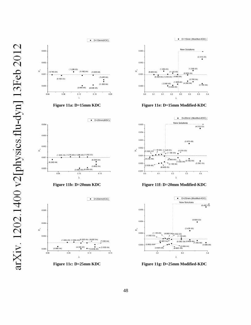
48
Figure 11a: D=15mm KDC Figure 11e: D=15mm Modified-KDC
Figure 11b: D=20mm KDC Figure 11f: D=20mm Modified-KDC
Figure 11c: D=25mm KDC Figure 11g: D=25mm Modified-KDC

49
Figure 11d: D=30mm KDC
Figure 11h: D=30mm Modified-KDC
Fig. 11 Values of calculated by KDC equation and its modified form from data of F&W in tubes of
four different diameters.
Each of the ‗new‘ solutions appears as a pair. As increases the separation in value between the pairs
increases for each tube. This is a consequence of the fact that the modification is larger for larger causing a
larger shift to lower values on the y-axis of Fig.4,thereby increasing the separation between the two roots. The
lowest ‗new‘ solution for , has one of the two values close to the correct value ( ); for
the lowest solution pair are equally spaced around correct ,with good accuracy ( in Fig.
11(g), ~25% in Fig. 11(f), ~40% and ~90% in Fig. 11(h)) Each of the 8 solutions at higher values of have one of
the two solutions close to the correct value, accuracy range being 25-80%. One of the two solutions in each case is
within at most a factor of 2 of the correct .
Modified KDC equation increases the range of and for which solutions of good accuracy can be
obtained. RRMSD with respect to ‗correct‘ value are: KDC: 0.465 and modified KDC: 0.322.
The values of the coefficients of the forth order polynomial in order of decreasing power of are:
[0.153338, -0.322906, 0.294622, 0.042879] for and [0.182216 0.267440 -0.661362 0.252113] for .
4.5.2 Low systems: Modified KDC equation improves the constancy of values of determined with different
and in experiments with Glycerol and Silicone oil. In these low systems the issue of multiple solutions
or of new solutions with modified KDC equation does not arise. The results are shown for Glycerol in Fig. 12(a)
(KDC) (Table 4) and in Fig. 12(b) (modified-KDC); for Silicone oil in Fig. 12(c) (KDC) (Table 4) and in Fig. 12(d)
(modified-KDC). The RRMSD with respect to the correct value of decreases from to for Glycerol
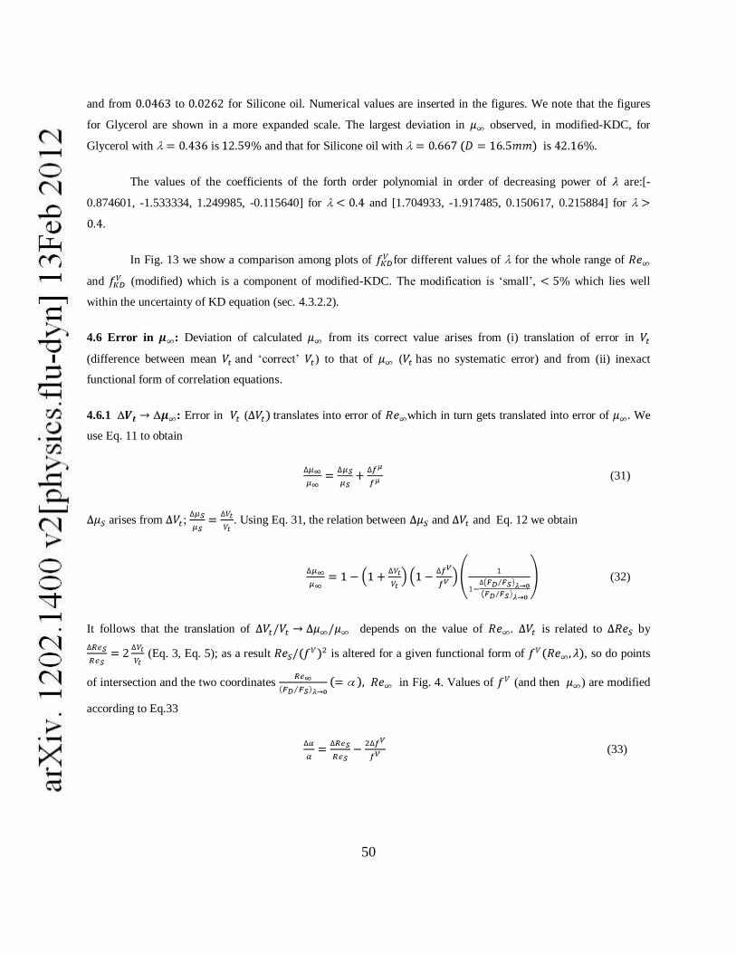
50
and from to for Silicone oil. Numerical values are inserted in the figures. We note that the figures
for Glycerol are shown in a more expanded scale. The largest deviation in observed, in modified-KDC, for
Glycerol with is and that for Silicone oil with is .
The values of the coefficients of the forth order polynomial in order of decreasing power of are:[-
0.874601, -1.533334, 1.249985, -0.115640] for and [1.704933, -1.917485, 0.150617, 0.215884] for
.
In Fig. 13 we show a comparison among plots of for different values of for the whole range of
and (modified) which is a component of modified-KDC. The modification is ‗small‘, which lies well
within the uncertainty of KD equation (sec. 4.3.2.2).
4.6 Error in : Deviation of calculated from its correct value arises from (i) translation of error in
(difference between mean and ‗correct‘ ) to that of ( has no systematic error) and from (ii) inexact
functional form of correlation equations.
4.6.1 : Error in ( translates into error of which in turn gets translated into error of We
use Eq. 11 to obtain
(31)
arises from ; . Using Eq. 31, the relation between and and Eq. 12 we obtain
(32)
It follows that the translation of depends on the value of . is related to by
(Eq. 3, Eq. 5); as a result is altered for a given functional form of , so do points
of intersection and the two coordinates in Fig. 4. Values of (and then ) are modified
according to Eq.33
(33)

51
Figure 12a: D=40mm; Glycerol; KDC
Figure 12c: D=40mm; Glycerol; Modified-KDC
Figure 12b: D=40, 30 and 16.5mm; Silicone oil;
KDC
Figure 12d: D=40, 30 and 16.5mm; Silicone oil;
Modified-KDC
Fig. 12: Values of calculated by KDC equation and its modified form for Glycerol & Silicone oil. data
are in Table 2. values are in Table 4.
We note that of Eq. 33, arising entirely from is defined in Eq. 23a, has negligible value and
can be ignored in Eq. 32 and 33. Table 15 and Fig. 14 shows propagation of error in to that in in different
ranges of and . The error is large for larger . The values stress the need to make highly accurate
measurements of with large ball-liquid combinations. The 22 ball-tube combinations for which no solutions
could be obtained have large and belong to the error-prone group.

52
Figure 13: for fixed value of as a function of original and modified form.
With we obtain (using Eq. 25)
(34)
4.6.2 Functional form error: The presence of error in the functional form of correlation equations generates a
contribution to and a non zero . We obtain
(35)
4.6.3 Error magnitudes: An increase in and with increasing and consequent increase in
is observed for low systems (sec. 4.2.9, Table 8). A value of is found to be error-prone.This error is
entirely functional form error. In large domain we again find larger relative deviation in calculated µ∞ (~33%,
~40%) for the largest entry in (Table 11), for which . values are also large ( ~2000). At
smaller and the deviations are , in some cases much smaller. The larger deviations in
the two smallest entries in Table 11arise from anomalous values of (sec. 4.4.8). In tubes with the
relative deviations are: ~7-16% and only for the two largest are ~50% and 180% respectively ( = 3910 and
7105 respectively); in , the relative deviations are: 17-34% for the first four entries and ~80% for the
largest ( = 7300) . The values of for which large and large and .are observed (Table
11) are considerably lower ( ~0.15) than the value range of error-prone (> 0.4) in the smaller range (<50).
for large is smaller than that for smaller , but so is ; the ratio in some cases is larger for large .
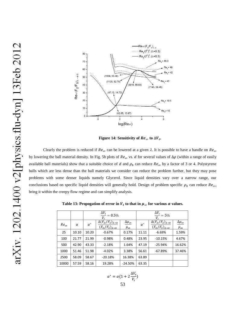
53
Figure 14: Sensitivity of to .
Clearly the problem is reduced if can be lowered at a given . It is possible to have a handle on
by lowering the ball material density. In Fig. 5b plots of vs. for several values of (within a range of easily
available ball materials) show that a suitable choice of and can reduce by a factor of 3 or 4. Polystyrene
balls which are less dense than the ball materials we consider can reduce the problem further, but they may pose
problems with some denser liquids namely Glycerol. Since liquid densities vary over a narrow range, our
conclusions based on specific liquid densities will generally hold. Design of problem specific can reduce ,
bring it within the creepy flow regime and can simplify analysis.
Table 13: Propogation of error in to that in for various values.
25 10.10 10.20 -0.67% 0.17% 11.11 -6.69% 1.59%
100 21.77 21.99 -0.98% 0.48% 23.95 -10.15% 4.67%
500 42.90 43.33 -2.18% 1.64% 47.19 -25.94% 16.62%
1000 51.46 51.98 -4.02% 3.38% 56.61 -67.89% 37.46%
2500 58.09 58.67 -20.18% 16.38% 63.89
10000 57.59 58.16 19.28% -24.50% 63.35

54
Conclusion
It is possible to extend the use of falling ball viscometry with excellent accuracy well beyond the ‗creepy flow‘
regime with use of the method described in this paper.
Acknowledgement
The work is based on the Master‘s theses of A. V. Singh and L. Sharma and subsequent work done by them as
Research Fellows at IIT Kanpur. They thank IIT Kanpur for the financial assistance. The authors also thank
Debiprasad Palit, Asoke Kumar Mallik, Vishal Saxena, Aloke Trivedi, S. Vishnu, Mitesh, Naresh, Saurabh Paul,
Subhrajyoti Adhya, V. Chandrasekhar, S. G. Dhande, R. N. Mukherjee, P.K. Bhardwaj, , Salman Khan, R. S.
Rajput, P. H. Tewari, Piyush Sahay, Sanghamitra Deb, Arunava Ghosh and. Anil Kumar Verma
References
1. Clift, R., Grace, J. , and Weber, M.E., (1978), Bubbles, Drops and Particles, Academic Press. New York: 1 Table 5.2,2 p 223
2. Happel, J. and Brenner, H. (1983), Low Reynolds number Hydrodynamics, Martinus Nijhoff , The Hague, p. 319a, 7-4
b
3. Kim, S. and Karrilla, S.J., (2005), Microhydrodynamics: Principles and Selected Applications, Dover Publications, New York.
4. Leach J, Mushfique H, Keen S, Di Leonardo R, Ruocco G, Cooper J M and Padgett M J, (2009), Comparison of Faxén's correction for
a microsphere translating or rotating near a surface. Physical review. E 79, 026301-4.
5. Kahle A, Winkler B , Hennion B., (2003), Is Faxén‘s correction function applicable to viscosity measurements of silicate melts with the
falling sphere method? J. Non-Newtonian Fluid Mech. 112 , 203–215
6. Kaiser A.E., Graham A.L and Mondy L.A. (2004), Non-Newtonian Wall Effects in Concentrated Suspensions J.Non-Newtonian Fluid
Mech., 116, 479-488.
7. Brizard M., Megharfi M., Mahé E. and Verdier C (2005), Design of a high precision falling ball viscosimeter Review of Scientific
Instruments, 76, 025109(1-6).
8. Feng S, Graham A.L., Reardon P.T., Abbott J., Mondy L.; (2006), Improving falling ball test for viscosity determination J. Fluid
Engineering,128, 157-163.
9. Ma Jing, Lopez-Pedrosa J. M, and Bradley M. (2008), High-throughput viscosity determinations Review of Scientific Instruments 79,
094102(1-7).
10. Kaji, N., Mori, Y. H., Tochitani, Y., Komotori, K. (1980), Augmentation of direct contact heat transfer to drops with an intermittent
electric field. Trans. ASME, 102, 32-37.
11. Scott, T. C.; Wham, R. M. (1988), Surface area generation and droplet size control in solvent extraction systems utilizing high intensity
electric fields. U.S. Patent 4767515.
12. Ptasinski, K. J.; Kerkhof, P. J. A. M. (1992), Electric field driven separations: Phenomena and applications. Sep. Sci. Technol., 27, 995-
1021.
13. Mordant N., Pinton J.F. (2000), Velocity measurement of a settling sphere. Eur. Phys. J. B., 18, 343-352.
14. TÖZeren. H. (1983), Drag on eccentrically positioned spheres translating and rotating in tubes, J. Fluid Mechanics , 129, 77-90.
15. Rubinow S.I. and Keller J. B. (1961), The transverse force on a spinning sphere moving in a viscous fluid J. of Fluid Mechanics, 11,
447-459.
16. Shinohara, M. and Hashimoto, H (1979), The lateral force on a small sphere sedimenting in a viscous fluid bounded by a cylindrical
wall J.Phys.Soc.Japan, 46, 320-327.
17. Ambari, A. Gauthier-Manuel,B.and E.Guyon (1984), Wall effects on a sphere translating at constant velocity, J. Fluid. Mech 149,235-
253.

55
18. Humphrey J. A. C. and Murata H.(1992), On the Motion of Solid Spheres Falling Through Viscous Fluids in Vertical and Inclined
Tubes J. Fluid Engineering, 114, 2-11.
19. Becker, L.E. McKinley, G.H. and Stone, H.A. (1996), Sedimentation of a Sphere Near a Plane Wall: Weak Non-Newtonian and Inertial
Effects J. of Non Newtonian Fluid Mechanics, 63, 201-233.
20. Bougas A. and Stamatoudis M. (1992), Wall factor for acceleration and terminal velocity of falling spheres at high reynolds numbers
Chemical Engineering & Technology, 16, 314 – 317.
21. Feng,J.,Huang ,P.Y., Joseph,D.D. (1996), The motion and interaction of solid particles in viscoelastic liquids J.of Non Newtonian Fluid
Mechanics, 63, 63-88.
22. Changfu Y, Haiying Q and Xuchang X (2003), Lift force on rotating sphere at low Reynolds numbers and high rotational speeds Acta
Mechanica Sinica, 19, 300-307.
23. Williams M. C. Normal stress and viscosity measurements for polymer solutions in steady cone-and-plate shear AIChE Journal, 11,
467 – 473.
24. Sutterby, J.L., (1966), Laminar converging flow of dilute polymer solutions in conical sections: Part I. Viscosity data, new viscosity
model tube flow solution. AIChE J., 12, 62–69.
25. Turian R.M. (1967), An experimental investigation of the flow of aqueous non-Newtonian high polymer solutions past a sphere AIChE
Journal ,13, 999 – 1006.
26. Caswell B. (1970), The effect of finite houndaries on the motion of particles innon-Newtonian fluids Chem. Eng. Science, 25, 1167-
1176.
27. Cygan, D. A.,Caswell,B. (1971), Precision Falling Sphere Viscometry Journal of Rheology, 15, 663-683.
28. Tran-Son-Tay R., Beaty B.B., Acker D.N., Hochmuth R.M. (1988), Magnetically driven, acoustically tracked, translating-ball
rheometer for small, opaque samples. Review Sci. Instrum, 59, 1399-1404.
29. Chhabra R. P. and Uhlherr P. H. T. (1979), Estimation of zero shear viscosity of polymer solutions from falling sphere data Rheol.
Acta, 18, 593- 599.
30. Barnes, H.A., (1995) A review of the slip (wall depletion) of polymer-solutions, emulsions and particle suspensions in viscometers-its
cause,character and cure, J. Non-Newtonian Fluid Mech, 56, 221-251.
31. Barnes, H.A. (2000), Measuring the viscosity of large-particle (and flocculated) suspensions- A note on the necessary gap size of
rotational viscometers, J. Non-Newtonian Fluid Mech, 94, 213-217.
32. Chhabra R P (2002) in Transport processes in bubbles drops and particles Ed. D. De Kee and RP Chhabra, Taylor and Francis New
York, London Second Edition, Chapter 13, p 316-337, p317a.
33. DiFelice, R., (1996a) A relationship for the wall effect on the settling velocity of a sphere at any flow regime. Int. J. Multiphase Flow,
22, 523-527.
34. Kehlenbeck R. and Di Felice R. (1999), Empirical Relationships for the Terminal Settling Velocity of Spheres in Cylindrical Columns
Chem. Eng. Technol.,21, 303-308.
35. Francis A.W.(1933), Wall Effect in Falling Ball Method for Viscosity; Physics; 4,403-406.
36. Fidleris V. and Whitmore R. L., (1961), Experimental determination of the wall effect for spheres falling axially in cylindrical vessels
Br. J. Appl. Phys., 12, 490-494.
37. McNown J.S., Lee H.M., McPherson M.B. and Ebgez S.M (1948), Proceedings of the 7th International Congress Appl.Mech, 2, 17-29.
38. Sutterby J.L. (1973a), Falling Sphere Viscometry. I. Wall and Inertial Corrections to Stokes‘ Law in Long Tubes Trans. Soc. Rheool.,
17, 559-575.
39. Proudman, I., and J. R. A. Pearson, J. Fluid Mechanics., 2 (1957), Expansions at small Reynolds numbers for the flow past a sphere and
a circular cylinder, 237-262.
40. Cheng, N.S. (2009), Comparison of formulas for drag coefficient and settling velocity of spherical particles, Powder Technol., 189,
395–398.
41. Wham,R.M.,Basaran,O.A.,and Byers ,C.H.(1996), Wall effects on Flow past solid spheres at finite Reynolds
numbers.Ind.Eng.Chem.Res.,35, 864-874.
56
42. Haberman, W.L. (1956), Ph.D. thesis, University of Maryland.
43. Paine, P.L. and Scherr, P(1975), Drag coefficients for the movement of rigid spheres through liquid-filled cylindrical pores. Biophys.
J., 15,1087-1091.
44. Coutanceau M. These d‘Etat, Universite de Poitiers, 1971.
45. Bohlin, T. (1960), On the drag on rigid spheres, moving in a viscous liquid inside cylindrical tubes, Trans. Roy. Inst. Technol.
(Stockholm), 155, 1-63.
46. Haberman, W. L. and R. M. Sayre (1958) Motion of Rigid and Fluid Spheres in Stationary and Moving Liquids Inside Cylindrical
Tubes. David Taylor Model Basin. Report No. 1143. U.S. Navy, Washington, D.C. (Formula cited in Chhabra (2002)).
47. Ambari A, Gauthier-Manuel B and Guyon. E. (1985), Direct measurement of the tube wall effect on the Strokes force Phys. Fluids, 28,
1559-1561.
48. Turton, R. Levenspiel, O. (1986) A short note on the drag correlation for spheres, Powder Technol. 47 83–86.
49. Brown, P.P. Lawler D.F. (2003) Sphere drag and settling velocity revisited, J. Envir. Engg.-ASCE, 129, 222–231.
50. Munroe, H. S. (1888) The english versus continental system of jigging—is close sizing advantageous? Trans. Am. Inst. Min. Engrs., 17
(1888), p. 637–657
51. Arsenijević, Z.Lj. Grbavčić, Ž.B. Garić-Grulović, R.V. Bošković-Vragolović, N.M. (2010), Wall effects on the velocities of a single
sphere settling in a stagnant and counter-current fluid and rising in a co-current fluid Powder Technology, 203,237-242.
52. Flude M J C and Daborn. J E (1982), Viscosity measurement by means of falling spheres compared with capillary viscometry. J. Phys.
E : Sci. Instrum,. 15, 1313-1321.
53. Fidleris V. and Whitmore R. L., (1959), Measurement of the falling velocity of particles in opaque fluids J of Scientific Inst., 36, 35-
36.
54. Subbaraman V., Mashelkar R. A., and Ulbrecht J. (1971), Extrapolation procedures for zero shear viscosity with a falling sphere
viscometer Rheol. Acta, 10, 429-433.
55. Christopherson D. G. and Dawson D. (1959), An example of energy dissipation in viscous flow, Proc. Roy. Soc. London. A 251,1267,
550-564.
56. Bungay P. M and Brenner H. (1973), The motion of a closely-fitting sphere in a fluid-filled tube, Int. J. Multiphase Flow, 1, . 25-56.