Embed Size (px)
Citation preview
TEL AVIV UNIVERSITYTHE RAYMOND AND BEVERLY SACKLER FACULTY OF EXACT SCIENCES
SCHOOL OF COMPUTER SCIENCE
STUDIES IN ALGEBRAIC ANDPROPOSITIONAL PROOF COMPLEXITY
Thesis Submitted for the Degree of Doctor of Philosophy
by
Iddo Tzameret
Under the supervision of
Professor Nachum Dershowitz and Professor Ran Raz
SUBMITTED TO THE SENATE OF TEL AVIV UNIVERSITY
AUGUST 2008


This work was carried out under the supervision ofProf. Nachum Dershowitz (Tel Aviv University) and Prof. Ran Raz (Weizmann Institute)


Contents
1 Introduction 11.1 Background on Propositional Proof Complexity . . . . . . . . . . . . . . 2
1.1.1 Concrete Proof Systems . . . . . . . . . . . . . . . . . . . . . . 31.1.2 Overview of Proof Systems . . . . . . . . . . . . . . . . . . . . 51.1.3 Comparing Proof Systems: Simulations and Separations . . . . . 6
1.2 Contribution of the Thesis . . . . . . . . . . . . . . . . . . . . . . . . . 71.2.1 Multilinear Proofs . . . . . . . . . . . . . . . . . . . . . . . . . 71.2.2 Resolution over Linear Equations with Applications to Multilinear
Proofs . . . . . . . . . . . . . . . . . . . . . . . . . . . . . . . . 111.2.3 Symbolic proofs of polynomial identities . . . . . . . . . . . . . 161.2.4 Propositional Proofs under a Promise . . . . . . . . . . . . . . . 20
2 Preliminaries 262.1 General Notations . . . . . . . . . . . . . . . . . . . . . . . . . . . . . . 27
2.1.1 CNF Formulas . . . . . . . . . . . . . . . . . . . . . . . . . . . 272.2 Resolution and Bounded-Depth Frege Proof Systems . . . . . . . . . . . 272.3 Basic Notions from Proof Complexity . . . . . . . . . . . . . . . . . . . 282.4 Algebraic Propositional Proof Systems . . . . . . . . . . . . . . . . . . . 292.5 Arithmetic and Multilinear Circuits and Formulas . . . . . . . . . . . . . 30
2.5.1 Arithmetic Circuits and Formulas . . . . . . . . . . . . . . . . . 302.5.2 Multilinear Polynomials, Circuits and Formulas . . . . . . . . . . 312.5.3 Notational Conventions Regarding Arithmetic Formulas . . . . . 322.5.4 Symmetric Polynomials . . . . . . . . . . . . . . . . . . . . . . 32
3 Multilinear Proofs 363.1 Basic Manipulations of Arithmetic Formulas . . . . . . . . . . . . . . . 393.2 Soundness and Completeness of fMC . . . . . . . . . . . . . . . . . . . 423.3 Simulation Results . . . . . . . . . . . . . . . . . . . . . . . . . . . . . 443.4 Separations of Algebraic Proof Systems and Multilinear Circuit Lower
Bounds . . . . . . . . . . . . . . . . . . . . . . . . . . . . . . . . . . . 473.5 Tseitin’s Graph Tautologies . . . . . . . . . . . . . . . . . . . . . . . . . 50
iii

Contents iv
3.5.1 Consequences: Separation Results . . . . . . . . . . . . . . . . . 553.6 Chapter Summary . . . . . . . . . . . . . . . . . . . . . . . . . . . . . . 56
4 Resolution over Linear Equations 574.1 R(lin) and its Fragments . . . . . . . . . . . . . . . . . . . . . . . . . . 58
4.1.1 Disjunctions of Linear Equations . . . . . . . . . . . . . . . . . . 584.1.2 Resolution over Linear Equations – R(lin) . . . . . . . . . . . . . 594.1.3 Fragment of Resolution over Linear Equations – R0(lin) . . . . . 60
4.2 Reasoning and Counting inside R(lin) and its Subsystems . . . . . . . . . 624.2.1 Basic Reasoning inside R(lin) and its Subsystems . . . . . . . . . 624.2.2 Basic Counting inside R(lin) and R0(lin) . . . . . . . . . . . . . 64
4.3 Implicational Completeness of R(lin) . . . . . . . . . . . . . . . . . . . . 674.4 Short Proofs for Hard Tautologies . . . . . . . . . . . . . . . . . . . . . 69
4.4.1 The Pigeonhole Principle Tautologies in R0(lin) . . . . . . . . . . 694.4.2 Tseitin mod p Tautologies in R0(lin) . . . . . . . . . . . . . . . . 724.4.3 The Clique-Coloring Principle in R(lin) . . . . . . . . . . . . . . 76
4.5 Interpolation Results for R0(lin) . . . . . . . . . . . . . . . . . . . . . . 804.5.1 Interpolation for Semantic Refutations . . . . . . . . . . . . . . . 814.5.2 Polynomial Upper Bounds on Interpolants for R0(lin) . . . . . . . 844.5.3 Feasible Monotone Interpolation . . . . . . . . . . . . . . . . . . 86
4.6 Size Lower Bounds . . . . . . . . . . . . . . . . . . . . . . . . . . . . . 874.7 Relations with Extensions of Cutting Planes . . . . . . . . . . . . . . . . 894.8 Chapter Summary . . . . . . . . . . . . . . . . . . . . . . . . . . . . . . 93
5 From Resolution over Linear Equations to Multilinear Proofs 945.1 From R(lin) Proofs to PCR Proofs . . . . . . . . . . . . . . . . . . . . . 955.2 From PCR Proofs to Multilinear Proofs . . . . . . . . . . . . . . . . . . 97
5.2.1 Multilinearization of Polynomials . . . . . . . . . . . . . . . . . 975.3 Applications to Multilinear Proofs: Small Depth-3 Multilinear Proofs . . 1025.4 Chapter Summary . . . . . . . . . . . . . . . . . . . . . . . . . . . . . . 103
6 Symbolic Proofs of Polynomial Identities 1056.1 Preliminaries . . . . . . . . . . . . . . . . . . . . . . . . . . . . . . . . 1066.2 Analytic Symbolic Proofs of Polynomial Identities . . . . . . . . . . . . 107
6.2.1 Depth-3 formulas and depth-3 analytic symbolic proofs . . . . . 1106.3 The Structure of Symbolic Proofs . . . . . . . . . . . . . . . . . . . . . 112
6.3.1 Regular Analytic Symbolic Proofs . . . . . . . . . . . . . . . . . 1136.4 Completeness . . . . . . . . . . . . . . . . . . . . . . . . . . . . . . . . 1166.5 Lower Bounds . . . . . . . . . . . . . . . . . . . . . . . . . . . . . . . . 117
6.5.1 Hard Formulas . . . . . . . . . . . . . . . . . . . . . . . . . . . 1186.5.2 Key Lemma: Lower Bounds on Deriving One Formula from Another118

Contents v
6.5.3 Main Lower Bound: Regular Depth-3 Proofs . . . . . . . . . . . 1226.5.4 Proof of Technical Lemma . . . . . . . . . . . . . . . . . . . . . 129
6.6 Chapter Summary . . . . . . . . . . . . . . . . . . . . . . . . . . . . . . 135
7 Propositional Proofs under a Promise 1367.1 Preliminaries and Notations . . . . . . . . . . . . . . . . . . . . . . . . . 137
7.1.1 Size-Width Tradeoffs . . . . . . . . . . . . . . . . . . . . . . . . 1377.1.2 Boolean Circuit Encoding . . . . . . . . . . . . . . . . . . . . . 137
7.2 Promise Proof Systems . . . . . . . . . . . . . . . . . . . . . . . . . . . 1387.2.1 Promise Axioms . . . . . . . . . . . . . . . . . . . . . . . . . . 1397.2.2 Promise Resolution . . . . . . . . . . . . . . . . . . . . . . . . . 1417.2.3 Discussion . . . . . . . . . . . . . . . . . . . . . . . . . . . . . 142
7.3 Big Promise: Upper Bound . . . . . . . . . . . . . . . . . . . . . . . . . 1437.4 Smaller Promise: Lower Bound . . . . . . . . . . . . . . . . . . . . . . 148
7.4.1 The Lower Bound . . . . . . . . . . . . . . . . . . . . . . . . . 1507.5 Appendix: Encodings . . . . . . . . . . . . . . . . . . . . . . . . . . . . 154
7.5.1 Encoding of Boolean Circuits and Promise Axioms . . . . . . . . 1547.6 Chapter Summary . . . . . . . . . . . . . . . . . . . . . . . . . . . . . . 158
8 Conclusions and Open Problems 159


List of Figures
6.1 Underlying graph of an analytic symbolic proof . . . . . . . . . . . . . . 114
vii

Abstract
The field of proof complexity aims at characterizing which statements have shortproofs in a given formal proof system. This thesis is a contribution to proof complex-ity broadly construed as the field that studies the sizes of structured or symbolic proofs.Our focus will be on the development and complexity-theoretic study of new frameworks,mainly of an algebraic nature, for providing, among other things, proofs of propositionaltautologies. We further link and motivate the proof systems we explore with certain ques-tions, mainly from algebraic complexity. The main results of this thesis can be dividedinto four parts, as follows.
MULTILINEAR PROOFS: We introduce an algebraic proof system that operates withmultilinear arithmetic formulas. We show that this proof system is fairly strong, even whenrestricted to multilinear arithmetic formulas of a very small depth. Specifically, we showthat algebraic proofs manipulating depth-2 multilinear arithmetic formulas polynomiallysimulate resolution, Polynomial Calculus (PC) and Polynomial Calculus with Resolution(PCR) proofs. We provide polynomial size proofs manipulating depth-3 multilinear arith-metic formulas for the pigeonhole principle tautologies and the Tseitin’s graph tautologies.
By known lower bounds, this demonstrates that algebraic proof systems manipulat-ing depth-3 multilinear formulas are strictly stronger than resolution, PC and PCR, andhave an exponential gap over bounded-depth Frege for both the pigeonhole principle andTseitin’s graph tautologies.
We illustrate a connection between lower bounds on multilinear proofs and lowerbounds on multilinear circuits. In particular, we show that (an explicit) super-polynomialsize separation between proofs manipulating general arithmetic circuits and proofs ma-nipulating multilinear circuits implies a super-polynomial size lower bound on multilinearcircuits for an explicit family of polynomials.
The short multilinear proofs for hard tautologies are established via a connection be-tween depth-3 multilinear proofs and extensions of resolution, described as follows:
RESOLUTION OVER LINEAR EQUATIONS WITH APPLICATIONS TO MULTILINEAR
PROOFS: We develop and study the complexity of propositional proof systems of varyingstrength extending resolution by allowing it to operate with disjunctions of linear equa-tions instead of clauses. We demonstrate polynomial-size refutations for hard tautologieslike the pigeonhole principle, Tseitin graph tautologies and the clique-coloring tautologiesin these proof systems. Using (monotone) interpolation we establish an exponential-sizelower bound on refutations in a certain, strong, fragment of resolution over linear equa-tions, as well as a general polynomial upper bound on (non-monotone) interpolants in thisfragment. We show that proofs operating with depth-3 multilinear formulas polynomi-ally simulate a certain, strong, fragment of resolution over linear equations (by which theaforementioned upper bounds on multilinear proofs follow). We then connect resolutionover linear equations with extensions of the cutting planes proof system.

SYMBOLIC PROOFS OF POLYNOMIAL IDENTITIES: To transform algebraic propo-sitional proof systems operating with arithmetic formulas into formal proof systems oneusually augments the system with an “auxiliary” proof system capable of manipulatingarithmetic formulas by means of the polynomial-ring axioms. We investigate basic struc-tural and complexity characterizations of the latter proof system and its fragments. Specif-ically, a symbolic proof for establishing that a given arithmetic formula Φ computes thezero polynomial (or equivalently, that two given arithmetic formulas compute the samepolynomial) is a sequence of formulas, starting with Φ and deriving the formula 0 bymeans of the standard polynomial-ring axioms applied to any subformula. We introducefragments of symbolic proofs named analytic symbolic proofs, enjoying a natural property:a symbolic proof is analytic if one cannot introduce arbitrary new formulas anywhere inthe proof (that is, formulas computing the zero polynomial which do not originate, in a pre-cise manner, from the initial arithmetic formula). We establish exponential lower boundson the number of steps in analytic symbolic proofs operating with depth-3 arithmetic for-mulas, under a certain regularity condition on the structure of proofs (roughly, mimickinga tree-like structure). The hard instances are explicit and rely on small formulas for thesymmetric polynomials.
ALTERNATIVE MODELS OF REFUTATION – PROMISE PROPOSITIONAL PROOFS: Westudy the problem of certifying unsatisfiability of CNF formulas under the promise thatany satisfiable formula has many satisfying assignments, where “many” stands for anexplicitly specified function Λ in the number of variables n. To this end, we developpropositional proof systems under different measures of promises (that is, different Λ) asextensions of resolution. This is done by augmenting resolution with axioms that, roughly,can eliminate sets of truth assignments defined by Boolean circuits. We then investigatethe complexity of such systems, obtaining an exponential separation in the average-casebetween resolution under different size promises: (i) Resolution has polynomial-size refu-tations for all unsatisfiable 3CNF formulas when the promise is ε ·2n, for any constant0 < ε < 1; (ii) There are no sub-exponential size resolution refutations for random 3CNFformulas, when the promise is 2δn (and the number of clauses isO(n3/2−ε), for 0 < ε < 1
2),
for any constant 0 < δ < 1.

Acknowledgements
First and foremost I would like to thank my supervisors Nachum Dershowitz and Ran Raz.I went with Nachum a long way since the days before I started my graduate studies, and Iam greatly indebted to his continuous support, interest, generosity, kindness and also his greatadvices and knowledge through all of this time. Ever since I met Ran, when I began mygraduate studies, his deep understanding and brilliant insights gave a tremendous push to myresearch and were invaluable in the course of my work. I was very fortunate to have him asmy advisor and I’m indebted to his great patience which led us to rather lengthy talks and forhis commitment to research which had a great impact on me. Ran constantly encouraged meto develop my research and to find new directions. His contribution to this thesis is invaluablein both his ideas and his strive toward complete thoroughness and clarity.
A very special thanks goes to Jan Krajıcek for inviting me to the Cambridge workshop onproof complexity, for the excellent yearly fall schools organized by him, and for his interest inmy work as well as his very useful comments. I believe that Jan’s book on bounded arithmeticand proof complexity was one of the main reasons I got interested in proof complexity in thefirst place.
I would also like to thank my friends and colleagues from the open-space, and espe-cially Amir Epstein and Zur Izhakian; and also colleagues with whom I met in numerousproof-complexity gatherings, and in particular Pavel Pudlak and other members and guests ofthe “Prague school”, among these are Marta Bılkova, Emil Jerabek, Leszek Kołodziejczyk,Phuong Nguyen, Jakob Nordstrom, Steven Perron and Neil Thapen.
I had very helpful discussions with Pavel Hrubes and Neil Thapen on some of the resultsin this thesis. For some results I’ve also benefited from discussions with Amnon Ta-Shma,whose versatile complexity courses were also of great help; and helpful correspondence withEli Ben-Sasson, Dima Grigoriev and Arist Kojevnikov. Thanks also to Sam Buss for sendingme a Xerox of his (out of print) seminal book. I thank Michael Ben-Or and Uri Zwick forserving in my thesis proposal committee, and Arnon Avron, Udi Boker, Yoram Hirshfeld,Alex Rabinovich, Boaz (Boris) Trakhtenbrot and Anna Zamansky for the opinionated logicseminars. Anonymous referees of some of my papers were of great help in improving theexposition of some of the material in this thesis. During my studies I was supported by theIsrael Science Foundation (grant no. 250/05). Last but not least, I wish to thank my parents fortheir constant support during the years of research.
Iddo Tzameret August 2008Tel Aviv, Israel


Chapter 1
Introduction
1

Chapter 1. Introduction 2
Proof complexity lies at the intersection of computational complexity and logic. Com-putational complexity aims at understanding the nature and limitations of efficient compu-tation; logic, on the other hand, and in particular proof theory, studies what can formally beproved from a given set of axioms and deduction rules, in a given language. Accordingly,proof complexity aims at characterizing which statements can formally be proved withefficient (or feasible) proofs. Here the term “efficient” typically stands for two separate(though interconnected) meanings: the first meaning refers to the size of the proofs, thatis, the number of symbols (or bits) it takes to write down the proofs. The second mean-ing refers to the efficiency of the “concepts” one reasons with (the technical interpretationbeing the complexity class from which proof-lines are taken).
Let us begin with a short introduction to the field of propositional proof complexity.
1.1 Background on Propositional Proof ComplexityPropositional proof complexity deals with proof systems that establish propositional tau-tologies. A propositional proof system is usually described by a finite set of inferencerules and axiom schemata. A propositional proof is then a derivation of some tautologythat applies the prescribed inference rules to the set of axioms. We can sometimes take thedual view in which proof systems establish that some formula is unsatisfiable by derivingFALSE from the formula and axioms. Thus, the proofs in such systems are usually calledrefutations.
The standard definition of a formal (or abstract) proof system in this setting is thatintroduced by Cook and Reckhow in their seminal work Cook and Reckhow (1979).
Definition 1.1.1 (Cook-Reckhow propositional proof system) A Cook-Reckhowpropositional proof system (or a formal propositional proof system) is a polynomial-timealgorithm A that receives a propositional formula F (most commonly a Boolean formulain the connectives ∨,∧,¬) and a string π over some finite alphabet (“the [proposed]proof” of F ), such that there exists a π with A(F, π) = 1 if and only if F is a tautology.
Note that the requirement of a formal proof system A is that proofs are polynomial-time recognizable (polynomial in the size of both the proofs π and the formulas F ). Thecompleteness of a (Cook-Reckhow) proof system (with respect to the set of all proposi-tional formulas; or for a subset of it, e.g. the set of tautological formulas in disjunctivenormal form [DNFs]) means that every tautological formula F has a string π (“the proofof F ”) so that A(F, π) = 1. The soundness of a (Cook-Reckhow) proof system meansthat for every formula F , if there is a string π for which A(F, π) = 1, then F is indeed atautology.
Given Definition 1.1.1, the basic question of propositional proof complexity is this:
Fix a formal propositional proof system P and a propositional tautology τ .What is the smallest proof of τ in P?

Chapter 1. Introduction 3
From the perspective of computational complexity, this question is of fundamental im-portance, since showing that for every propositional proof system P , there are tautologiesτ with no polynomial-size (in the size of τ ) proofs in P , would readily imply NP 6= coNP,as was observed in Cook and Reckhow (1979).
From the perspective of algorithmics (and computational logic), establishing lowerbounds on the size of proofs in certain proof systems, usually gives lower bounds on therun-time of specific procedures for NP-complete problems like certain SAT-solvers andtheorem provers (cf. Impagliazzo et al. (1999); Beame et al. (2002); Segerlind (2007a)).These run-time lower bounds are rather broad, in the sense that they do not depend onspecific heuristics taken by the procedures for solving the problems.
Furthermore, from the perspective of mathematical logic, and specifically the proof-and model-theoretic study of formal (first, or higher-order) systems of arithmetic, tight andsignificant connections with propositional proof complexity were discovered. To someextent, propositional proofs are the non-uniform counterpart of weak formal systems ofarithmetic (generally called theories of bounded arithmetic); in fact, lower bounds onpropositional proof systems are closely related to independence (that is, unprovability)results in weak systems of arithmetic (cf. Buss (1986); Krajıcek (1995); Razborov (1996);Buss (1997); Cook (2005); Cook and Nguyen (2004–2008)).
Yet another aspect of propositional proof complexity is its tight relation – in spiritand techniques – to circuit complexity. It seems that there is a correspondence betweenproving lower bounds on a circuit class and proving lower bounds on proofs operating withcircuits of the prescribed circuit class, though formal and specific relations between proofcomplexity hardness and computational hardness are quite restricted currently (see Beameand Pitassi (1998) for a short discussion on circuit-complexity based proof systems; seealso Segerlind (2007b) for a technical survey of propositional proof complexity).
In what follows we focus on concrete proof systems that are usually studied in theproof complexity literature and which are relevant to this thesis.
1.1.1 Concrete Proof Systems
Perhaps the most natural and typical family of proof systems are those systems originatingin mathematical logic, which are called Frege proof systems (or Hilbert-style proof sys-tems). When considering only the propositional fragment of this family of proof systems,we obtain a textbook proof system, in which each proof-line1 is usually a Boolean formulawith the logical connectives ∧,∨,¬, which stand for AND, OR, NOT, respectively (and,optionally, the implication connective→). A proof in a Frege system is a sequence of for-mulas that starts from a set of self-evident (and easily recognizable) axioms and derivesnew formulas (that is, new proof-lines) by using a set of self-evident deduction rules. Inthis way, the proof system enables one to derive any propositional tautology (and onlypropositional tautologies).
1Each element (usually a formula) of a proof-sequence is referred to as a proof-line.

Chapter 1. Introduction 4
Algebraic proof systems. In the course of investigating the complexity of differentpropositional proof systems, connections were found between proofs operating withBoolean formulas and proofs operating with multivariate polynomials over a fixed field(cf. Beame et al. (1996); Pitassi (1997)). Proof systems operating with polynomials arecalled algebraic proof systems. In this setting one replaces logical reasoning (as used inFrege proofs), with basic algebraic reasoning. Specifically, in algebraic proofs one usuallystarts from a set of polynomials, with the intended semantics that each of the polynomialsevaluates to 0 over the field, and by using simple algebraic deduction rules like addition oftwo polynomials and multiplication of a polynomial by a variable, derives new polynomi-als (from previous ones). Such algebraic proofs usually demonstrate that a collection ofpolynomial equations has no solutions (that is, no common roots) over some fixed field.When the collections of initial polynomial equations are derived from propositional con-tradiction (most typically, from the clauses of unsatisfiable formulas in conjunctive normalform [CNF]) and the algebraic proofs establish that the collections have no 0, 1 solutionsover the field, then the proof system is called an algebraic propositional proof system.
The Polynomial Calculus proof system (PC, for short), introduced in Clegg et al.(1996), is a well studied algebraic (propositional) proof system. Fix some field F andlet Q be a collection of multivariate polynomial equations Q1 = 0, . . . , Qm = 0, whereeach Qi is taken from the ring of polynomials F[x1, . . . , xn]. In PC the fact that the col-lection Q has no 0, 1 solutions over the field F is proved by using the following basicalgebraic inference rules: from two polynomials p and q (interpreted as the two equationsp = 0 and q = 0) we can deduce α · p + β · q, where α, β are elements of F; and fromp we can deduce xi · p, for any variable xi (1 ≤ i ≤ n). A sequence of polynomials thatuses Q1, . . . , Qm and x2
i −xi (for any variable xi) as initial polynomial equations, followsthe above algebraic inference rules, and terminates with 1 (with the intended semanticsbeing that 1 evaluates to 0; thus, 1 here stands for FALSE), is called a PC refutation of thepolynomial (equations) Q1, . . . , Qm.
It can be shown by Hilbert’s Nullstellensatz that for every unsatisfiable set of polyno-mials (unsatisfiable, in the sense that the polynomials have no common 0, 1 roots over thefield) there exists a PC refutation. Also, since the deduction rules are sound, every deriva-tion of the polynomial 1 must start from a set of unsatisfiable set of polynomials, and sooverall we obtain a sound and complete proof system that can establish the unsatisfiabilityof every unsatisfiable set of polynomials over the field.
When we consider algebraic proof systems we have the possibility to relax somewhatthe notion of a proof : instead of requiring that a proof be polynomially-verifiable (as isrequired by the definition of a formal proof system), we may only require that the proofwill be polynomially-verifiable with high probability. This is done by considering theproofs as being semantic proofs (this semantic setting was first considered by Pitassi inPitassi (1997)). In other words, each proof-line can be regarded as (the set of solutions of)a (formal) multivariate polynomial over the given field; and where each such polynomialis written as an arbitrarily chosen arithmetic formula computing the polynomial (note thata single polynomial might have many representation as an arithmetic formula). Some ofthe algebraic proof systems we study in this thesis are semantic proof systems. We shall

Chapter 1. Introduction 5
also study ways to turn semantic algebraic proofs into syntactic ones (that is, into formalpropositional proof systems – verifiable in deterministic polynomial time).
Besides the fact that algebraic proof systems are almost as natural as their Booleancounterparts (that is, Frege proof systems), there are many other motivations for studyingalgebraic proofs. In fact, the initial interest in algebraic proof systems arose due to theirconnections with Frege proof systems operating with constant-depth formulas equippedwith modular counting gates and Frege proofs operating with constant-depth formulasaugmented with modular counting axioms (cf. Beame et al. (1996); Buss et al. (1996/97);Beame and Riis (1998); Impagliazzo and Segerlind (2001, 2002)). Proving lower boundson constant depth Frege proof with counting gates is still an important open problemin proof complexity theory. Another motivation for considering algebraic proof systemis more akin to questions of practical importance, for instance, boosting performance inautomatic theorem provers and SAT-solvers by using algebraic reasoning (see for exampleClegg et al. (1996); Hirsch et al. (2005)).
In this thesis we study algebraic proof systems as objects of interest in their own right,and we shall also consider their connections with questions in algebraic complexity andalgebraic circuit complexity.
1.1.2 Overview of Proof Systems
We now list the proof (and refutation) systems we consider in this thesis. Some of the proofsystems have already been considered in previous works and other systems are introducedin this thesis (we shall define these formally in the relevant places).
Algebraic propositional proof systems. Polynomial Calculus, denoted PC (introducedin Clegg et al. (1996)). A proof system for the set of unsatisfiable CNF formulas written asan unsatisfiable set of polynomial equations over a field. Each polynomial in a PC proofis represented as an explicit sum of monomials.
Polynomial Calculus with Resolution, denoted PCR (introduced in Alekhnovich et al.(2002)). This is an extension of PC where for each variable xi a new formal variablexi is added. The variable xi equals 1−xi. Each polynomial in a PCR proof is representedas an explicit sum of monomials. PCR can polynomially simulate both PC and resolution.
Formula Multilinear Calculus, denoted fMC. The fMC is a semantic algebraic proposi-tional proof system for the set of unsatisfiable CNF formulas written as unsatisfiable setof multilinear polynomial equations over a field. Each polynomial in an fMC proof is amultilinear polynomial represented as a multilinear arithmetic formula (we consider arith-metic formulas that can use unbounded fan-in + (addition) and × (product) gates).
Depth-k Formula Multilinear Calculus, denoted depth-k fMC. This is a restriction of fMCto multilinear arithmetic formulas of depth at most k.
The cMC and cPCR proof systems. The cMC proof system is similar to fMC, exceptthat multilinear polynomials are represented by multilinear arithmetic circuits (instead of
Chapter 1. Introduction 6
multilinear arithmetic formulas). In the same manner, cPCR is a proof system similar toPCR, except that polynomials are represented by (general) arithmetic circuits (instead ofsums of monomials).
Proof systems operating with Boolean formulas. Resolution (introduced by Blake(1937) and further developed in Robinson (1965)). A proof system for establishing theunsatisfiability of CNF formulas. Each resolution proof-line consists of a clause (i.e., adisjunction of variables or their negations). The last line of a resolution refutation is theempty clause, which has no satisfying assignment.
Bounded-depth Frege. This system is usually considered as a proof system for the set ofBoolean tautologies. The lines in a bounded depth Frege proof consists of constant-depthformulas over the connective NOT and the unbounded fan-in connectives AND, OR. Wecan consider bounded-depth Frege to be also a proof system for the set of unsatisfiableBoolean formulas, by treating a proof sequence (starting from some initial set of unsatis-fiable formulas) that ends with FALSE, as a refutation.
Propositional proofs under a promise. These are refutation systems operating withBoolean formulas (or clauses, in case we deal with extensions of resolution) that are com-plete and sound for the set of formulas promised to be either unsatisfiable or to havesufficiently many satisfying assignments (where the term “sufficiently many” stands foran explicitly given function of the number of variables in the formula).
Boolean-Algebraic proof systems. Resolution over linear equations (R(lin), for short)and its fragments. The R(lin) proof system establishes unsatisfiable CNF formulas. EachR(lin) proof-line consists of a disjunction of linear equations with integer coefficients (thecoefficients are written in unary notation). The last line of an R(lin) refutation is the emptyclause, which has no satisfying assignment. We shall also define a (provably weaker)fragment of R(lin), denoted R0(lin).
Extensions of the cutting planes proof system. The R(CP*) proof system (introduced inKrajıcek (1998)) is a common extension of resolution and CP* (the latter is cutting planeswith polynomially bounded coefficients). The system R(CP*) is essentially resolutionoperating with disjunctions of linear inequalities (with polynomially bounded integralcoefficients) augmented with the cutting planes inference rules.
Algebraic proof systems for polynomial identities. Symbolic proofs of polynomialidentities. A symbolic proof for establishing that a given arithmetic formula Φ com-putes the zero polynomial (or equivalently, that two given arithmetic formulas computethe same polynomial) is a sequence of formulas, starting with Φ and deriving the formula0 by means of the standard polynomial-ring axioms applied to any subformula.
Chapter 1. Introduction 7
1.1.3 Comparing Proof Systems: Simulations and Separations
For two propositional proof systems P1, P2 we say that P2 polynomially simulates P1 iffor every propositional formula F and every P1-proof π of F , there exists a proof of F inP2 of size polynomial in the size of π. In case P2 polynomially simulates P1 while P1 doesnot polynomially simulate P2 we say that P2 is strictly stronger than P1 or that there isa (super-polynomial) separation of P2 and P1. In case a proof system P uses a languagethat is different language from the set of Boolean propositional formulas, we shall fixahead a simple (and efficient) translation that maps Boolean propositional formulas to thelanguage used by P (and this way we can treat the proof system P as a proof system forthe set of Boolean propositional formulas).
In this thesis, when comparing the strength of different propositional proof systems,we shall restrict ourselves to CNF formulas only. That is, we consider propositional proofsystems such as resolution and bounded-depth Frege as proof systems for the set of un-satisfiable CNF formulas and we consider algebraic proof systems to be proof systems forthe set of polynomial translations of unsatisfiable CNF formulas (see Section 2.4). Moreformally:
Definition 1.1.2 (Simulations and separations) Let P1, P2 be two proof systems for theset of unsatisfiable CNF formulas. We say that P2 polynomially simulates P1 if given aP1 refutation π of a CNF F , there exists a refutation of F in P2 of size polynomial in thesize of π. In case P2 polynomially simulates P1 while P1 does not polynomially simulateP2 we say that P2 is strictly stronger than P1 and also that there is a (super-polynomial)separation of P2 and P1. Given an unsatisfiable CNF formula F , we say that P2 has anexponential gap over P1 for F , if there exists a polynomial size P2 refutation of F , andthe smallest P1 refutation of F is of exponential size. If either P1 or P2 are algebraicproof systems, then we identify the CNF formula F with its translation to a collection ofpolynomial equations.
For the sake of convenience we shall sometimes write simply simulates to mean poly-nomially simulates. Since we do not talk about other concepts of simulations, there shouldbe no confusion.
1.2 Contribution of the ThesisThe thesis is divided basically into the following four parts: multilinear proofs, resolutionover linear equations, symbolic proofs of polynomial identities and propositional proofsunder a promise. The following subsections elaborate on these four parts.
1.2.1 Multilinear Proofs
In Chapter 3 we introduce a natural family of algebraic proof systems generally calledmultilinear proof systems. In particular we consider an algebraic proof system Formula

Chapter 1. Introduction 8
Multilinear Calculus (fMC) that manipulates multilinear arithmetic formulas. A multi-linear proof (that is, an fMC proof) begins with an initial set of multilinear polynomialequations representing the clauses of a CNF formula (where a polynomial is multilinearif in each of its monomials the power of every variable is at most one), and the goal isto prove that the CNF formula is unsatisfiable by showing the equations have no 0, 1solutions over a given fixed field.
Specifically, let Q be a set of initial multilinear polynomial equations in the formalvariables x1, . . . , xn, x1, . . . , xn over some fixed field. A multilinear proof of the insolv-ability of Q is a sequence of multilinear polynomial equations, where each polynomial isrepresented as (an arbitrarily chosen) multilinear arithmetic formula (a multilinear arith-metic formula is an arithmetic formula in which every gate computes a multilinear polyno-mial). The sequence uses the initial equations plus the polynomial equations xi+xi−1 = 0and xi · xi = 0 (for all variables xi, xi) as axioms, and terminates with the unsatisfiableequation 1 = 0. Derivations of polynomial equations in the sequence are done by applyingthe following two basic algebraic inference rules to previous equations in the sequence:
• from p = 0 and q = 0 one can deduce α · p+ β · q = 0, where α, β are elements ofthe field;
• from p = 0 one can deduce q · p = 0 , for any polynomial q such that q · p ismultilinear.
(The inclusion of the equalities xi + xi− 1 = 0 and xi · xi = 0 forces the variables xi andxi to take on only the Boolean values 0 and 1, where xi takes the negative value of xi.) Ifsuch a sequence exists then there is no assignment of 0, 1 values that satisfies all the initialequations. Such a proof of insolvability is then called a multilinear refutation of the initialpolynomial equations.
We can obtain in this way a proof system for (unsatisfiable) CNF formulas. Given aCNF formula F in the variables x1, . . . , xn we translate F to a system of multilinear poly-nomial equations in the variables x1, . . . , xn, x1, . . . , xn. Each clause C of F translatesinto a multilinear polynomial equation qC = 0. F is satisfiable if and only if the systemof polynomial equations qC = 0, for all clauses C of F , has a common root in the field,where the root also satisfies the axioms xi + xi − 1 = 0 and xi · xi = 0 (for all variablesxi, xi). For example, the CNF (x1 ∨x2 ∨¬x3)∧ (¬x2 ∨x4) translates into the polynomialequations x1 · x2 · x3 = 0 , x2 · x4 = 0.
The minimal refutation size of a given set of initial polynomial equations (i.e., thenumber of symbols that it takes to write down the refutation of these equations) is thestandard measure for the strength of an algebraic proof system. In algebraic proof systemssuch as the Polynomial Calculus (PC) (described above) and Polynomial Calculus withResolution (PCR), one represents the polynomials inside refutations as explicit sum ofmonomials. Then, the size of a PC or a PCR refutation is defined as the total number ofall monomials appearing in the refutation. On the other hand, in the multilinear proof sys-tem we present, polynomials inside refutations are represented as multilinear arithmetic

Chapter 1. Introduction 9
formulas. Accordingly, the size of a multilinear refutation is defined to be the total size ofall the multilinear arithmetic formulas appearing in the refutation.
Our results show that algebraic proof systems manipulating multilinear arithmetic for-mulas – and further, very small depth multilinear arithmetic formulas – constitute ratherstrong proof systems that are strictly stronger than PC, PCR and resolution. Moreover,such multilinear proof systems are capable of refuting efficiently (negations of) familiesof tautologies that were found hard2 for other proof systems, such as the bounded-depthFrege proof system. Furthermore, we illustrate a link between multilinear proofs and mul-tilinear arithmetic circuit lower bounds.
1.2.1.1 Background and Motivations
There is a great amount of literature devoted to proving lower bounds on the maximaldegree of polynomials appearing in PC refutations of some set of initial polynomials (cf.Razborov (1998), Impagliazzo et al. (1999), Buss et al. (2001), Ben-Sasson and Impagli-azzo (1999), Alekhnovich et al. (2004), Alekhnovich and Razborov (2001), Razborov(2002-2003)). These lower bounds imply a lower bound on the size of the refutations onlywhen polynomials are represented as a sum of monomials, that is, as depth-2 arithmeticformulas. For instance, Impagliazzo et al. (1999) showed that any degree lower bound thatis linear in the number of variables implies an exponential lower bound on the number ofmonomials in the refutation.
With respect to lower bounds on the refutation size of algebraic proof systems otherthan PC and PCR (in which the size of refutations is measured by the number of mono-mials appearing in the refutations), not much is known. Moreover, extending the PCproof system by allowing it to manipulate general (i.e., not necessarily multilinear) arith-metic formulas makes this proof system considerably stronger (cf. Buss et al. (1996/97);Pitassi (1997); Grigoriev and Hirsch (2003)). In particular, such an extended PC proofsystem that manipulates general arithmetic formulas polynomially simulates the entireFrege proof system, which is regarded as a rather strong proof system, and for which nosuper-polynomial size lower bounds are currently known. Thus, if one seeks to provesize lower bounds on refutation size, it is more reasonable to concentrate on (apparentlyweaker) extensions of PC (and PCR).
Furthermore, it is well known in proof complexity theory (cf. Beame and Pitassi(1998)) that there is an (informal) correspondence between circuit-based complexityclasses and proof systems based on these circuits (that is, proofs in which the prooflines consist of circuits from the prescribed circuit-class). Moreover, super-polynomialsize lower bounds on proofs manipulating circuits from a given circuit-class were onlyfound after super-polynomial size lower bounds were already proved for circuits fromthe circuit-class itself. Keeping in mind this correspondence, it is important to note thatsuper-polynomial lower bounds on multilinear arithmetic formulas for the determinant
2Given a proof system P and a family of tautologies τn | n ∈ N, we say that τn is hard for P in casethere is no P -proofs of τn of size polynomial in the size of τn (or equivalently, if there is no polynomial-sizeP -refutations of ¬τn).
Chapter 1. Introduction 10
and permanent functions, as well as other functions, were recently proved in Raz (2004,2006) and Aaronson (2004). On the other hand no super-polynomial lower bounds areknown for general arithmetic formulas.
In light of the aforesaid, our results show that algebraic proof systems operating withmultilinear arithmetic formulas (even of a very small depth) constitute on the one handfairly strong proof systems extending PC and PCR — and on the other hand, the cor-responding circuit-class (i.e., multilinear formulas) does have known super-polynomiallower bounds.
Moreover, as mentioned above, the correspondence between proof systems and circuit-classes is not a formal one, but instead it acts more as a working conjecture in proof com-plexity theory. Nevertheless, using multilinear proofs we are able to pinpoint an interestingcase where this correspondence can be formulated explicitly.
1.2.1.2 Summary of Results and Organization
In Chapter 3 we introduce the multilinear proof systems. We prove three kinds of re-sults. The results of the first kind are polynomial simulations. The second kind of resultsconcerns the problem of proving multilinear arithmetic circuit size lower bounds in con-nection to multilinear proof systems. The results of the third kind are upper bounds on therefutation size of combinatorial principles that were found hard for other proof systems.Both the simulations and upper bounds results are valid when one restricts the multilin-ear arithmetic formulas in the refutations to depth at most 3. Specifically, we show thefollowing.
Simulation results: In Chapter 3 (Sections 3.2 and 3.3) we show that Depth-2 fMCpolynomially simulates resolution, PC and PCR.
In Chapter 3 (Section 3.3) we provide a general simulation result for multilinearproofs. Specifically, Let S be a sequence of polynomials (not formulas) that forms aPCR proof sequence for some given set Q of multilinear polynomials, and consider thecorresponding sequence S ′ of multilinear polynomials formed by “multilinearization” (seeDefinition 2.5.2) of the polynomials in S. Then, the general simulation result essentiallysays that there is an fMC proof of Q of size polynomial in the total size of all the multilin-ear formulas that compute the polynomials in S ′.
Relations with algebraic circuit complexity: In Chapter 3 (Section 3.4) we utilizethe general simulation described above to assert the following: proving (an explicit) super-polynomial size separation between algebraic proofs manipulating general arithmetic cir-cuits and algebraic proofs manipulating multilinear arithmetic circuits implies a super-polynomial size lower bound on multilinear arithmetic circuits for an explicit family ofpolynomials.
Upper bounds: In Chapter 3 Section 3.5 we demonstrate the following upper bound:
1. Depth-3 fMC has polynomial-size refutations of the Tseitin mod p contradictions(for any p) over fields of characteristic q - p that include a primitive p-th root ofunity.

Chapter 1. Introduction 11
In Chapter 5 we establish more upper bounds on multilinear proofs of hard tautologies.This is accomplished as a consequence of a general simulation result (Corollary 5.2.5)stating that depth-3 multilinear proofs polynomially simulate a certain considerably strongfragment of resolution over linear equations introduced in Chapter 4. Specifically, weshow the following:
2. Depth-3 fMC over fields of characteristic 0 has polynomial-size refutations of thepigeonhole principle;
3. Depth-3 fMC has polynomial-size refutations of the Tseitin mod p contradictions(for any p) over any field of characteristic 0.
The short multilinear proofs of Tseitin mod p contradictions established in Chapter 3(Section 3.5) are different from the short proofs of Tseitin mod p demonstrated in Chapter5. The latter apply to multilinear proofs over any field of characteristic 0, while the formerover fields of characteristic q - p that include a primitive p-th root of unity. On the otherhand, the former proofs have the advantage of being more direct since they do not relyon small depth-3 representations of the symmetric polynomials (and so it is not knownif the latter proofs can be carried out in a “syntactic” multilinear proof system [see thediscussion on syntactic versus semantic algebraic proof systems in Section 1.2.3]).
Some consequences. Haken (1985) has shown an exponential lower bound on the sizeof resolution refutations of the pigeonhole principle. Moreover, exponential lower boundson the size of resolution refutations of certain Tseitin mod 2 tautologies (that is, Tseitintautologies based on expanding graphs) are also known (see Urquhart (1987); Ben-Sassonand Wigderson (2001)). We conclude then that depth-3 fMC is exponentially strongerthan resolution.
From the known exponential lower bounds on PC and PCR refutation size of certainTseitin mod p tautologies (cf. Buss et al. (2001); Ben-Sasson and Impagliazzo (1999);Alekhnovich et al. (2004)), we conclude that depth-3 fMC is strictly stronger than PC andPCR.
Note also that Razborov (1998) and subsequently Impagliazzo et al. (1999) haveshown an exponential-size lower bound on the size of PC (and PCR) refutations of alow-degree version of the pigeonhole principle. Our depth-3 fMC upper bound is alsoapplicable to this low-degree version (see Section 5.3 for more details on this).
Exponential lower bounds on the size of bounded-depth Frege proofs of the pigeon-hole principle were proved in Pitassi et al. (1993) and, independently, in Krajıcek et al.(1995). Thus Item (2) above shows an exponential gap of depth-3 fMC over boundeddepth Frege for the pigeonhole principle. Similarly, an exponential lower bound on thesize of bounded-depth Frege proofs of certain Tseitin mod 2 tautologies was shown inBen-Sasson (2002). Thus, Items (1) and (3) above implies that also for these Tseitin mod2 tautologies, depth-3 fMC has an exponential gap over bounded-depth Frege proofs.
The results on multilinear proofs appeared as parts of:
Chapter 1. Introduction 12
Ran Raz and Iddo Tzameret. The strength of multilinear proofs. Compu-tational Complexity, 17(3):407–457, 2008.
Ran Raz and Iddo Tzameret. Resolution over linear equations and multi-linear proofs. Ann. Pure Appl. Logic, 155(3):194–224, 2008.
1.2.2 Resolution over Linear Equations with Applications to Multi-linear Proofs
The resolution system is a popular refutation proof system for establishing the unsatisfi-ability of CNF formulas. Nevertheless, it is well known that resolution cannot providesmall, polynomial-size, proofs for many basic counting arguments. The most notable ex-amples of this are the strong exponential lower bounds on the resolution refutation size ofthe pigeonhole principle and its different variants. Due to the popularity of resolution bothin practice, as the core of many automated theorem provers, and as a theoretical case-studyin propositional proof complexity, it is natural to consider weak extensions of resolutionthat can overcome its inefficiency in providing proofs of counting arguments. In Chapter4 we present proof systems that are extensions of resolution, of various strengths, thatare suited for this purpose. In Chapter 5, these proof systems will be furthered linked tomultilinear proofs.
The basic proof system we shall study in Chapter 4 is denoted R(lin). The proof-lines in R(lin) proofs are disjunctions of linear equations with integral coefficients overthe variables ~x = x1, . . . , xn. It turns out that (already proper subsystems of) R(lin) canhandle very elegantly basic counting arguments. The following defines the R(lin) proofsystem. Given an initial CNF, we translate every clause
∨i∈I xi ∨
∨j∈J ¬xj (where I
are the indices of variables with positive polarities and J are the indices of variables withnegative polarities) pertaining to the CNF, into the disjunction
∨i∈I(xi = 1)∨∨j∈J(xj =
0). Let A and B be two disjunctions of linear equations, and let ~a · ~x = a0 and ~b · ~x = b0
be two linear equations (where ~a,~b are two vectors of n integral coefficients, and ~a · ~x isthe scalar product
∑ni=1 aixi; and similarly for ~b · ~x). The rules of inference belonging
to R(lin) allow to derive A ∨ B ∨ ((~a − ~b) · ~x = a0 − b0) from A ∨ (~a · ~x = a0) andB ∨ (~b ·~x = b0). We can also simplify disjunctions by discarding (unsatisfiable) equationsof the form (0 = k), for k 6= 0. In addition, for every variable xi, we shall add an axiom(xi = 0) ∨ (xi = 1), which forces xi to take on only Boolean values. A derivation ofthe empty disjunction (which stands for FALSE) from the (translated) clauses of a CNFis called an R(lin) refutation of the given CNF. This way, every unsatisfiable CNF hasan R(lin) refutation (this can be proved by a straightforward simulation of resolution byR(lin)).
The basic idea that enables us, in Chapter 5, to connect resolution operating with dis-junctions of linear equations and multilinear proofs is this: whenever a disjunction oflinear equations is simple enough—and specifically, when it is close to a symmetric func-tion, in a manner made precise—then it can be represented by a small size and small

Chapter 1. Introduction 13
depth multilinear arithmetic formula over large enough fields. We show how to polyno-mially simulate with multilinear proofs, operating with small depth multilinear formulas,certain short proofs carried inside resolution over linear equations. This enables us toprovide polynomial-size multilinear proofs for certain hard tautologies.
More specifically, we introduce a fragment of R(lin), which can be polynomially sim-ulated by depth-3 multilinear proofs (that is, proofs in depth-3 fMC). On the one hand thisfragment of resolution over linear equations already is sufficient to formalize in a transpar-ent way basic counting arguments, and so it admits small proofs of the pigeonhole prin-ciple and the Tseitin mod p formulas (which yields upper bounds on multilinear proofs);and on the other hand we can use the (monotone) interpolation technique to establish anexponential-size lower bound on refutations in this fragment as well as demonstrating ageneral (non-monotone) polynomial upper bound on interpolants for this fragment.
In Chapter 4 (Section 4.7) we consider the relation of the cutting planes system andits extensions with the R(lin) proof system. The cutting planes proof system operates withlinear inequalities with integral coefficients, and this system is very close to the extensionsof resolution we will study in Chapter 4. In particular, the following simple observationcan be used to polynomially simulate cutting planes proofs with polynomially boundedcoefficients (and some of its extensions) inside resolution over linear equations: the truthvalue of a linear inequality ~a ·~x ≥ a0 (where ~a is a vector of n integral coefficients and ~x isa vector of n Boolean variables) is equivalent to the truth value of the following disjunctionof linear equalities:
(~a · ~x = a0) ∨ (~a · ~x = a0 + 1) ∨ · · · ∨ (~a · ~x = a0 + k) ,
where a0 + k equals the sum of all positive coefficients in ~a (that is, a0 + k =max~x∈0,1n (~a · ~x)).
1.2.2.1 Comparison to Earlier Work
To the best of our knowledge our results are the first that consider the complexity of reso-lution proofs operating with disjunctions of linear equations. Previous works consideredextensions of resolution over linear inequalities augmented with the cutting planes infer-ence rules (the resulting proof system denoted R(CP)). In full generality, we show thatresolution over linear equations can polynomially simulate R(CP) when the coefficientsin all the inequalities are polynomially bounded (however, the converse is not known tohold). On the other hand, we shall consider a certain fragment of resolution over linearequations, in which we do not even know how to polynomially simulate cutting planesproofs with polynomially bounded coefficients in inequalities (let alone R(CP) with poly-nomially bounded coefficients in inequalities). We now discuss the previous work onR(CP) and related proof systems.
Extensions of resolution to disjunctions of linear inequalities were first considered inKrajıcek (1998) who developed the proof systems LK(CP) and R(CP). The LK(CP) sys-tem is a first-order (Gentzen-style) sequent calculus that operates with linear inequalitiesinstead of atomic formulas and augments the standard first-order sequent calculus infer-ence rules with the cutting planes inference rules. The R(CP) proof system is essentially
Chapter 1. Introduction 14
resolution over linear inequalities, that is, resolution that operates with disjunctions oflinear inequalities instead of clauses.
The main motivation of Krajıcek (1998) was to extend the feasible interpolation tech-nique and consequently the lower bounds results, from cutting planes and resolution tostronger proof systems. That paper establishes an exponential-size lower bound on a re-stricted version of R(CP) proofs, namely, when the number of inequalities in each proof-line isO(nε), where n is the number of variables of the initial formulas, ε is a small enoughconstant and the coefficients in the cutting planes inequalities are polynomially bounded.
Other papers considering extensions of resolution over linear inequalities are the morerecent papers by Hirsch and Kojevnikov (2006) and Kojevnikov (2007). The first paperHirsch and Kojevnikov (2006) considers combinations of resolution with LP (an incom-plete subsystem of cutting planes based on simple linear programming reasoning), with the‘lift and project’ proof system (L&P), and with the cutting planes proof system. That pa-per also illustrates polynomial-size refutations of the Tseitin mod 2 tautologies in all theseextensions of resolution. The second paper Kojevnikov (2007) deals with improving theparameters of the tree-like R(CP) lower-bounds obtained in Krajıcek (1998). Also, on themore practical level, Hirsch, Itsykson, Kojevnikov, Kulikov, and Nikolenko (2005) havedeveloped an experimental SAT-solver (that is, a software tool for deciding satisfiabil-ity) named basolver, which stands for mixed Boolean-Algebraic Solver. This SAT-solversolves CNF formulas (and also checks Boolean circuits for equivalence) by translatingthem first into systems of polynomial equations and disjunctions of polynomial equations,and then solving these systems by means of derivation rules in the spirit of the resolutionderivation rules.
Whereas previous results concerned primarily with extending the cutting planes proofsystem, our foremost motivation is to link resolution over linear equations to multilinearproofs. As mentioned above, motivated by relations with multilinear proofs operating withdepth-3 multilinear formulas, we shall consider a certain subsystem of resolution over lin-ear equations. For this subsystem we apply twice the interpolation by a communicationgame technique. The first application is of the non-monotone version of the technique,and the second application is of the monotone version. Namely, the first application pro-vides a general (non-monotone) interpolation theorem that demonstrates a polynomial (inthe size of refutations) upper bound on interpolants; The proof uses the general methodof transforming a refutation into a Karchmer-Wigderson communication game for twoplayers, from which a Boolean circuit is then attainable. In particular, we shall apply theinterpolation theorem of Krajıcek (1997). The second application of the (monotone) inter-polation by a communication game technique is implicit and proceeds by using the lowerbound criterion of Bonet, Pitassi, and Raz (1997). This criterion states that (semantic)proof systems (of a certain natural and standard kind) whose proof-lines (considered asBoolean functions) have low communication complexity cannot prove efficiently a certaintautology (namely, the clique-coloring tautologies).

Chapter 1. Introduction 15
1.2.2.2 Summary of Results and Organization
The proof systems. In Chapter 4 we formally define two extensions of resolution ofdecreasing strength allowing resolution to operate with disjunctions of linear equations.The size of a linear equation a1x1 + . . . + anxn = a0 is in fact Σn
j=0 |aj|, where |aj| isthe size of the coefficients aj written in unary notation. The size of a disjunction of linearequations is the total size of all linear equations in the disjunction. The size of a proofoperating with disjunctions of linear equations is the total size of all the disjunctions in it.
R(lin): This is the stronger proof system (described above) that operates with disjunc-tions of linear equations with integer coefficients.
R0(lin): This is a (provably proper) fragment of R(lin). It operates with disjunctionsof (arbitrarily many) linear equations whose variables have constant coefficients, underthe restriction that every disjunction can be partitioned into a constant number of sub-disjunctions, where each sub-disjunction either consists of linear equations that differ onlyin their free-terms or is a (translation of a) clause.3 For the precise definition see Section4.1.3.
Note that any single linear inequality with Boolean variables can be represented by adisjunction of linear equations that differ only in their free-terms (see the example men-tioned above in this section). So the R0(lin) proof system is close to a proof system op-erating with disjunctions of constant number of linear inequalities (with constant integralcoefficients). In fact, disjunctions of linear equations varying only in their free-terms, havemore (expressive) strength than a single inequality. For instance, the PARITY function canbe easily represented by a disjunction of linear equations, while it cannot be representedby a single linear inequality (nor by a polynomial-size disjunction of linear inequalities).
As already mentioned, the motivation to consider the restricted proof system R0(lin)comes from its relation to multilinear proofs operating with depth-3 multilinear formu-las: R0(lin) corresponds roughly to the subsystem of R(lin) that we know how to simulateby depth-3 multilinear proofs (the technique is based on converting disjunctions of linearforms into symmetric polynomials, which are known to have small depth-3 multilinearformulas). This simulation is then applied in order to obtain upper bounds on depth-3multilinear proofs, as R0(lin) is already sufficient to efficiently prove certain “hard tau-tologies”. Moreover, we are able to establish an exponential lower bound on R0(lin) refu-tations size (see below for both upper and lower bounds on R0(lin) proofs). We alsoestablish a super-polynomial separation of R(lin) from R0(lin) (via the clique-coloringprinciple, for a certain choice of parameters; see below).
Upper bounds. In Chapter 4 we demonstrate the following short refutations in R0(lin)and R(lin):
1. Polynomial-size refutations of the pigeonhole principle in R0(lin);
3The free-term of a linear form a1x1 + . . .+ anxn + a0 is a0.
Chapter 1. Introduction 16
2. Polynomial-size refutations of Tseitin mod p graph formulas in R0(lin);
3. Polynomial-size refutations of the clique-coloring formulas in R(lin) (for certain pa-rameters). The refutations here follow by direct simulation of the Res(2) refutationsof clique-coloring formulas from Atserias et al. (2002).
Interpolation results. In Chapter 4 Section 4.5 we provide a polynomial upper-boundon (non-monotone) interpolants corresponding to R0(lin) refutations; Namely, we showthat any R0(lin)-refutation of a given formula can be transformed into a (non-monotone)Boolean circuit computing the corresponding interpolant function of the formula (if thereexists such a function), with at most a polynomial increase in size. We employ the generalinterpolation theorem for semantic proof systems from Krajıcek (1997).
Lower bounds. In Chapter 4 Section 4.6 we provide the following exponential lowerbound:
Theorem 1.2.1 R0(lin) does not have sub-exponential refutations for the clique-coloringformulas.
This result is proved by applying a result of Bonet, Pitassi, and Raz (1997). The resultin Bonet et al. (1997) (implicitly) use the monotone interpolation by a communicationgame technique for establishing an exponential-size lower bound on refutations of generalsemantic proof systems operating with proof-lines of low communication complexity.
Relations with cutting planes proofs. A proof system combining resolution with cut-ting planes was presented in Krajıcek (1998). The resulting system is denoted R(CP)(see Section 4.7 for a definition). When the coefficients in the linear inequalities insideR(CP) proofs are polynomially bounded, the resulting proof system is denoted R(CP*). InChapter 4 Section 4.7 we establish the following simulation result:
Theorem 1.2.2 R(lin) polynomially simulates resolution over cutting planes inequalitieswith polynomially bounded coefficients R(CP*).
We do not know whether the converse simulation holds.
From resolution over linear equations to multilinear proofs. Chapter 5 is devoted toestablish the following theorem, connecting multilinear proofs with resolution over linearequations:
Theorem 1.2.3 Multilinear proofs operating with depth-3 multilinear formulas over char-acteristic 0 polynomially-simulate R0(lin).

Chapter 1. Introduction 17
An immediate corollary of this theorem and the upper bounds in R0(lin) described inChapter 4 are the polynomial-size multilinear proofs for the pigeonhole principle and theTseitin mod p formulas.
The results on resolution over linear equations appeared as parts of:
Ran Raz and Iddo Tzameret. Resolution over linear equations and multi-linear proofs. Ann. Pure Appl. Logic, 155(3):194–224, 2008.
1.2.3 Symbolic proofs of polynomial identities: From Semantic toSyntactic Algebraic Proofs
Let F be a field (say, the complex numbers) and let Φ be an arithmetic formula in the inputvariables x1, . . . , xn, computing a polynomial in the ring of polynomials F[x1, . . . , xn]. Asymbolic operation is any transformation of a subformula in Φ into another subformula,by means of the standard polynomial-ring axioms (expressing associativity and commu-tativity of both addition and multiplication, distributivity of multiplication over addition,equalities involving only field elements and the laws for the 0 and 1 elements in the field).
Chapter 6 deals with the following basic question:
How many symbolic operations does one need to perform on Φ in order tovalidate that Φ computes the zero polynomial?
To this end we define the notion of symbolic proofs of polynomial identities as follows:assume that the arithmetic formula Φ computes the zero polynomial, then a symbolic proofof this fact is a sequence of arithmetic formulas, where the first formula is Φ, the lastformula is the formula 0, and every formula in the sequence (excluding the first one) isderived from the (immediate) previous formula in the sequence by a symbolic operation.We are interested in the number of proof-lines in such proof sequences.
1.2.3.1 Background
The problem of deciding whether a given arithmetic circuit (or formula) over some fieldcomputes the zero polynomial – namely, the polynomial identity testing problem (PIT,for short) – is of great importance in algebraic complexity theory, and complexity theoryin general. It is known that when the underlying field is big enough there is an effi-cient probabilistic procedure for deciding whether an arithmetic circuit computes the zeropolynomial (cf. Schwartz (1980); Zippel (1979)). However, not much is known about thecomplexity of deterministic algorithms for this problem. Devising an efficient determin-istic procedure, or even demonstrating (non-deterministic) sub-exponential witnesses, forthe polynomial identity testing problem is a fundamental open problem.
The importance and apparent difficulty in finding an efficient deterministic procedure(or sub-exponential non-deterministic witnesses for that matter) for PIT led researchers toseveral different directions. On the one hand, there is a growing body of work dedicated
Chapter 1. Introduction 18
to establishing efficient deterministic procedures for PIT when arithmetic circuits are re-placed by more restrictive models of computing polynomials (cf. Raz and Shpilka (2005);Dvir and Shpilka (2006); Kayal and Saxena (2007); Karnin and Shpilka (2008); Shpilkaand Volkovich (2008)). On the other hand, in a somewhat more logical vein, evidence or“justifications” for the apparent empirical difficulty in finding efficient deterministic algo-rithms for PIT were discovered in Kabanets and Impagliazzo (2004) (see also, Dvir et al.(2008)).
In Chapter 6 we propose a different direction of research, relevant both to the poly-nomial identity testing problem as well as to proof complexity. Instead of studying algo-rithms for the PIT we shall concentrate on symbolic proofs of polynomial identities, thatis, proof sequences that manipulate formulas and which have clear and natural structure(besides the fact that they can be efficiently recognized). On the one hand, the choice tostudy proofs instead of algorithms gives the model more strength (in comparison to al-gorithms), as one can use non-determinism. On the other hand, we will restrict severelythe “reasoning” allowed in these proofs, and this will in turn enable us to demonstrateexponential-size lower bounds on certain proofs of polynomial identities.
1.2.3.2 Motivations
As discussed above, research into the complexity of symbolic proofs of polynomial iden-tities is directed, among others, to achieve better understanding of the polynomial identitytesting problem: although it is reasonable to assume (and widely believed) that there arepolynomial size witnesses (or “proofs”) of polynomial identities, lower bounds on certainsymbolic proofs of polynomial identities might lead to better understanding of the struc-ture of proofs needed in order to efficiently prove polynomial identities. On the applicativelevel, our work can be regarded as a contribution to the understanding of the efficiency ofsymbolic manipulation systems (like symbolic mathematical software tools). Neverthe-less, perhaps the most concrete motivation for studying symbolic proofs of polynomialidentities comes from algebraic proof systems, as we now explain.
From semantic to syntactic algebraic proof systems. Algebraic propositional proofsystems, as discussed before, and as we study in this thesis, are intended to demonstratethat a collection of polynomial equations, derived from the clauses of an unsatisfiableformula has no 0, 1 solutions over the fixed field.
In previous chapters (Chapters 3, 5) we dealt with semantic algebraic propositionalproof systems (and not syntactic ones), in which every proof-line is written as an arith-metic formula (or circuit). A semantic algebraic proof is a sequence of arithmetic for-mulas such that each formula in the sequence computes a formal multivariate polyno-mial (i.e., an element of the polynomial-ring F[x1, . . . , xn], where F is the base field andx1, . . . , xn are the formal variables of the system); note however that for every polynomialp ∈ F[x1, . . . , xn] there is no unique arithmetic formula computing p. Thus, each polyno-mial in the algebraic proof can be written in more than one way as an arithmetic formula.The inference of new polynomials from previous ones, via the algebraic inference rules,
Chapter 1. Introduction 19
is a semantic inference of polynomials from preceding ones, rather than a syntactic infer-ence of formulas from preceding formulas (for instance, the two inference rules mentionedabove are semantic in the sense that every root of p in F is also a root of q · p in F [forevery polynomial q]; and every common root of p and q in F is also a root of α · p+ β · q,for any α, β ∈ F).
It follows from the aforesaid that semantic algebraic proofs operating with arithmeticformulas might not necessarily be recognizable in polynomial-time (in the sizes of theproofs): because no polynomial-time procedure for the polynomial identity testing prob-lem is known, no known polynomial-time procedure can verify that a proof-line in analgebraic proof was derived correctly from preceding lines in the proof (for instance, thepolynomial p might be written as two completely different arithmetic formulas in a proof-line consisting of p and in its legitimate consequence consisting of q · p).
Nevertheless, it is sometimes preferable to turn to algebraic proofs that are polynomial-time recognizable. The most natural choice here is to join together the underlying semanticalgebraic proof system that operates with arithmetic formulas over a field (similar to thatmentioned above), with a symbolic proof system for establishing polynomial identities.This can be achieved, for instance, in the following simple manner: a syntactic algebraicproof is defined now to be a sequence of arithmetic formulas in which each proof-line iseither (i) an initial formula; or (ii) was derived from a previous formula in the sequenceby one of the derivation rules pertaining to the symbolic proof system (expressing thepolynomial-ring axioms, applied to any subformula); or (iii) was derived by the followinginference rules that correspond to the rules of the underlying algebraic proof system: fromthe formulas ϕ and ψ derive the formula α×ϕ+β×ψ (for α, β field elements); and fromthe formula ϕ derive the formula ψ × ϕ for any arithmetic formula ψ over the base field(the symbol × stands for the product gate).
Such natural syntactic algebraic propositional proof systems (operating with arithmeticformulas) were mentioned in Buss et al. (1996/97) and were explicitly introduced in Grig-oriev and Hirsch (2003). Understanding the complexity of symbolic proofs of polynomialidentities is essential in order to understand such syntactic algebraic propositional proofsystems operating with arithmetic formulas. Moreover, establishing super-polynomiallower bounds on symbolic proofs of polynomial identities might yield a super-polynomialseparation between semantic and syntactic algebraic (propositional) proof systems. Forinstance, the short (depth-3) multilinear proofs of hard tautologies established in Chapters5 use in an essential way the fact that the algebraic proof systems are semantic, and itis not known whether such short proofs exist for corresponding syntactic algebraic proofsystems.
1.2.3.3 The Basic Model: Analytic Symbolic Proofs
Recall the underlying model of symbolic proofs of polynomial identities illustrated above.We now explain the fragment of symbolic proofs we shall study here. With analogy to tra-ditional research in proof complexity (as well as classical proof theory and automatedproofs), we will consider symbolic proof systems that enjoy a property, which is anal-

Chapter 1. Introduction 20
ogous to some extent with the so-called subformula property in standard (propositionalor predicate sequent calculus) proofs. The subformula property states that every formulathat appears in a proof sequence π of T also appears in T . Intuitively, this means that theprover is forbidden from introducing notions not already present in the statement to beproved. Proofs having the subformula property are sometimes called analytic (or cut-freein the framework of the sequent calculus), and we shall adopt this term here.
Accordingly, we will introduce a proof system for the set of arithmetic formulas com-puting the zero polynomial, called analytic symbolic proofs, in which the following (re-laxed form of the) subformula property holds: if π is a proof sequence intended to establishthat the formula Φ computes the zero polynomial, then every subformula that appears insome proof-line in π is “originated” from the initial formula to be proved. More formally,this means that for every proof-line and every monomial (with its coefficient) that is syn-tactically computed in the proof-line, the same monomial is also syntactically computedin the initial proof-line (see Section 6.2 for more details on this and for the definition ofsyntactic computation of monomials).
The analytic criterion thus implies, for instance, that one cannot add arbitrary formulascomputing the zero polynomial in the proof (for example, one cannot get from the proof-line ϕ to the proof-line ϕ+ f − f , where f is some arbitrarily chosen arithmetic formula).
The (analytic) proof system we introduce is a natural proof system since, first, sym-bolic manipulations of polynomial formulas according to the polynomial-ring axioms issomething familiar to every high-school student, and second, the restriction to analyticproofs forbids only “ingenious” steps as illustrated above (that is, adding a formula f − f ,and then using in some clever way this f to efficiently derive the formula 0 in the system).
1.2.3.4 Results
The main technical result in Chapter 6 is an exponential-size lower bound on analyticsymbolic proofs of certain hard formulas computing the zero polynomial, where proofsoperate with depth-3 formulas and conform to a certain regularity condition on the struc-ture of proofs.
The hard formulas we provide are based on small depth-3 formulas for the elementarysymmetric polynomials. We establish a lower bound rate of 2Ω(
√`), where ` is the number
of variables in the initial hard formulas.The regularity condition intends to keep the following requirement: once a proof-line
A×(B+C) is transformed into the proof-lineA×B+A×C, in no way the two formulasA × B and A × C, as well as any other two formulas that originate (among others) fromA × B and A × C (in a manner made precise), be united together again into a productformula by means of the distributivity rule. For instance, in our case, after A × (B + C)was broken into the two sums A×B+A×C, these two sums (A×B and A×C) cannotbe united together again into a product formula by means of the “backward” distributivityrule, to yield A× (B + C), once more.
Our lower bound follows by a structural analysis of symbolic proofs, and specifically,by tracing the “paths” in which monomials and subformulas “move” along the proof.

Chapter 1. Introduction 21
Some basic algebraic properties of the small depth-3 formulas of the elementary symmet-ric polynomials are also exploited in the lower bound argument.
The results in this chapter appear in:
Iddo Tzameret. On the Structure and Complexity of Symbolic Proofs ofPolynomial Identities. Manuscript, 35 pages, April 2008.4
1.2.4 Propositional Proofs under a Promise
Any standard sound and complete propositional proof system has the ability to separatethe set of unsatisfiable formulas in conjunctive normal form (CNF) from the set of CNFformulas having at least one satisfying assignment, in the sense that every unsatisfiableCNF has a refutation in the system, while no satisfiable CNF has one. In Chapter 7 wedevelop and study, within the framework of propositional proof complexity, systems thatare “sound and complete” in a relaxed sense: they can separate the set of unsatisfiable CNFformulas from the set of CNF formulas having sufficiently many satisfying assignments(where the term “sufficiently many” stands for an explicitly given function of the numberof variables in the CNF). We call such proof systems promise refutation systems, as theyare complete and sound for the set of CNF formulas promised to be either unsatisfiable orto have many satisfying assignments.
Our first task in Chapter 7 is to introduce a natural model for promise propositionalrefutation systems. This is accomplished by augmenting standard resolution (or any otherpropositional proof system extending resolution) with an additional collection of axioms,the promise axioms. Each refutation in a promise refutation system can make use of atmost one promise axiom. The promise axioms are meant to capture the idea that wecan ignore or “discard” a certain number of truth assignments from the space of all truthassignments, and still be able to certify (due to the promise) whether or not the given CNFis unsatisfiable. The number of assignments that a promise axiom is allowed to discarddepends on the promise we are given, and, specifically, it needs to be less than the numberof assignments promised to satisfy a given CNF (unless it is unsatisfiable).
Assuming we have a promise that a satisfiable CNF has more than Λ satisfying assign-ments, we can discard up to Λ assignments. We refer to Λ as the promise. This way, therefutation system is guaranteed not to contain refutations of CNF formulas having morethan Λ satisfying assignments, as even after discarding (at most Λ) assignments, we stillhave at least one satisfying assignment left. On the other hand, any unsatisfiable CNFformula has a refutation in the system, as resolution already has a refutation of it.
We now explain what it means to “discard” assignments and how promise axiomsformulate the notion of discarding the correct number of truth assignments. Essentially,we say that a truth assignment ~a is discarded by some Boolean formula if ~a falsifies theformula. More formally, let X := x1, ..., xn be the set of underlying variables of agiven CNF, called the original variables. Let A be some CNF formula in the variables
4Independently of this paper, Pavel Hrubes recently investigated close problems concerning equationalsystems (Hrubes (2008)); the two papers are about to be substantially expanded and merged.

Chapter 1. Introduction 22
X , and assume that A also contains variables not from X , called extension variables.Let ~a ∈ 0, 1n be a truth assignment for the X variables, and assume that there is noextension of ~a (assigning values to the extension variables) that satisfies A. Thus, anyassignment satisfying A must also satisfy X 6≡ ~a (that is, A |= X 6≡ ~a), and so any(implicationally) complete proof system can prove X 6≡ ~a from A, or, in the case of arefutation system, can refute X ≡ ~a, given A. In this case, we say that the assignment ~ais discarded by A.
The promise axioms we present enjoy two main properties:
1. They discard assignments from the space of possible assignments to the variablesX .
2. They express the fact that not too many assignments to the variables X are beingdiscarded (in a manner made precise).
The first property is achieved as follows: let C be any Boolean circuit with n outputbits. Then we can formulate a CNF formula A (using extension variables) expressing thestatement that the output of C is (equal to) the vector of variables X . This enables Ato discard every truth assignment to the variables of X that is outside the image of theBoolean map defined by C, because, if an assignment ~a to X is not in the image of C,then no extension of ~a can satisfy A—assuming the formulation of A is correct. (Fortechnical reasons, the actual definition is a bit different from what is described here; seeSection 7.2.)
The second property is achieved as follows: assume we can make explicit the statementthat the domain of the map defined by the Boolean circuitC above is of size at least 2n−Λ.(See Section 7.2 in Chapter 7 for details on this.) Then, for the second property to hold, itis sufficient that the axiom formulates the statement that the circuit C defines an injectivemap (and thus the image of the map contains enough truth assignments), which can bedone quite naturally.
Given a certain promise and its associated promise axiom, we call a refutation ofresolution, augmented with the promise axiom, a resolution refutation under the (given)promise.
Besides introducing the model of promise refutation systems, our second task in Chap-ter 7 will be to investigate the basic properties of this model and in particular to determineits average-case proof complexity with respect to different sizes of promises (see belowfor a summary of our findings in this respect).
1.2.4.1 Background and Motivation
A natural relaxation of the problem of unsatisfiability certification is to require that, if aCNF is satisfiable, then it actually has many satisfying assignments. As mentioned above,we call the specific number of assignments (as a function of the number of variables n)required to satisfy a satisfiable CNF formula, the “promise”. It is thus natural to askwhether giving such a promise can help in obtaining shorter proofs of unsatisfiability.

Chapter 1. Introduction 23
It is possible to define an abstract promise proof system in an analogous manner tothe definition of an abstract (or formal) proof system (Definition 1.1.1). Nevertheless,as we already discussed in previous sections, proof complexity theory usually deals withspecific and structured proof systems. In accordance with this, we shall be interestedin Chapter 7 not with abstract proof systems (that is, not with finding general witnessesfor unsatisfiability, possibly under a promise), but rather with specific and more structuredproof systems, and specifically with refutation systems built up as extensions of resolution.
In the case of a big promise, that is, a constant fraction of the space of all truth as-signments (Λ = ε · 2n, for a constant 0 < ε < 1), there is already a deterministicpolynomial-time algorithm for any fixed natural number k that certifies the unsatisfiabilityof all unsatisfiable kCNF formulas under the promise: the algorithm receives a kCNF thatis either unsatisfiable or has more than Λ satisfying assignments and answers whether theformula is unsatisfiable (in case the formula is satisfiable the algorithm provides a satisfy-ing assignment). See Hirsch (1998); Trevisan (2004) for such efficient algorithms.5 Thistrivially implies the existence of polynomial-size witnesses for any unsatisfiable kCNFunder the promise ε · 2n. But does resolution already admit such short witnesses of unsat-isfiability (that is, resolution refutations) under a big promise? We show that the answer ispositive (for all unsatisfiable 3CNF formulas).
In the case of a smaller promise, by which we mean Λ = 2δn for a constant 0 <δ < 1, it is possible to efficiently transform any CNF over n variables to a new CNFwith n′ = dn/(1 − δ)e variables, such that the original CNF is satisfiable if and only ifthe new CNF has at least 2δn
′ satisfying assignments.6 Thus, the worst-case complexityof certifying CNF unsatisfiability under such a promise is polynomially equivalent to theworst-case complexity of certifying CNF unsatisfiability without a promise. However, it isstill possible that a promise of 2δn might give some advantage (that is, a super-polynomialspeedup over refutations without a promise) in certifying the unsatisfiability of certain (butnot all) CNF formulas; for instance, in the average-case.7
Feige, Kim, and Ofek (2006) have shown that when the number of clauses is Ω(n7/5)there exist polynomial-size witnesses for the unsatisfiability of 3CNF formulas in theaverage-case. On the other hand, Beame, Karp, Pitassi, and Saks (2002) and Ben-Sassonand Wigderson (2001) showed that resolution does not provide sub-exponential refutationsfor 3CNF formulas in the average-case when the number of clauses is at most n(3/2)−ε, forany constant 0 < ε < 1/2. 8 This shows that general witnessing of 3CNF unsatisfiability
5In the case the promise is Λ = 2n/poly(n), the algorithm in Hirsch (1998) also gives a deterministicsub-exponential time procedure for unsatisfiability certification of kCNF formulas (for a constant k).
6This can be achieved simply by adding new (n′ − n) “dummy variables”. For instance, by adding theclauses of a tautological CNF in these dummy variables to the original CNF. This way, if the original CNFhas at least one satisfying assignment then the new CNF has at least 2n
′−n ≥ 2δn′
satisfying assignments.7Note that if we add dummy variables to a 3CNF then we obtain an “atypical instance” of a 3CNF. Thus,
assuming we have polynomial-size witnesses of unsatisfiability of 3CNF formulas under a small promise inthe average-case (that is, the “typical case”), the reduction alone (that is, adding dummy variables) does notautomatically yield polynomial-size witnesses for 3CNF formulas in the average-case without a promise aswell.
8Beame et al. (2002) showed such a lower bound for n(5/4)−ε number of clauses (for any constant
Chapter 1. Introduction 24
is strictly stronger than resolution refutations. But is it possible that, under a promise of2δn, resolution can do better in the average-case? We show that the answer is negative.
There are two main motivations for studying propositional proofs under a givenpromise and their complexity. The first is to answer the natural question whether CNFunsatisfiability certification enjoys any advantage given a certain promise. As alreadymentioned, the answer is positive when the promise is a constant fraction of all the truthassignments, and our results imply that this phenomenon already occurs for resolution.For a small promise of 2δn, we can show that, at least in the case of resolution refutationsof most 3CNF formulas (of certain clause-to-variable density), the answer is negative. Infact, we can show that the answer stays negative even when the promise is bigger than2δn, and specifically when Λ = 2n/2n
ξ for some constant 0 < ξ < 1. Overall, our resultsestablish the first unsatisfiability certification model in which a promise of a certain givensize is known to help (that is, allow more efficient certifications) in the average-case, whilepromises of smaller sizes do not help.
The second motivation is more intrinsic to proof complexity theory: it is a generalgoal to develop natural frameworks for propositional proofs that are not sound in thestrict sense, but rather possess an approximate notion of soundness (like showing thatcertain “approximations” give speed-ups). For this purpose, the proof systems we proposeformalize—in a natural way—the notion of separating unsatisfiable CNF formulas fromthose that have many satisfying assignments. The promise axioms we present also allowfor a natural way of controlling the size of the promise, which in addition leads to anexponential separation between different size promises.
Chapter 7 develops the notion of propositional proofs under a promise, analyzes theproof complexity of these proof systems, as well as obtaining a separation, with respectto different promise sizes, and also illustrates several new facts about the resolution proofsystem.
1.2.4.2 Results and Organization
After defining the notion of proofs under a promise in Chapter 7 Section 7.2, we show thatresolution refutations are already enough to efficiently separate unsatisfiable 3CNF for-mulas from those 3CNF formulas with an arbitrarily small constant fraction of satisfyingassignments. In particular, in Section 7.3, we show the following:
Upper Bound: Let 0 < ε < 1 be any constant and let Λ = ε·2n be the given promise.Then every unsatisfiable 3CNF with n variables has a polynomial-size (in n) resolutionrefutation under the promise Λ.
The proof of this resembles a deterministic algorithm of Trevisan (2004) for approxi-mating the number of satisfying assignments of kCNF formulas.
0 < ε < 1/4). Ben-Sasson and Wigderson (2001) introduced the size-width tradeoff that enables one toprove an exponential lower bound for random 3CNF formulas with n(3/2)−ε number of clauses (for anyconstant 0 < ε < 1/2), but the actual proof for this specific clause-number appears in Ben-Sasson (2001).
Chapter 1. Introduction 25
In contrast to the case of a big promise, our results show that, at least for resolution, asmall promise of Λ = 2δn (for any constant 0 < δ < 1) does not give any advantage overstandard resolution (that is, resolution without the promise axioms) in most cases (that is,in the average-case). Specifically, in Section 7.4 we show the following:
Lower Bound: Let 0 < δ < 1 be any constant and let Λ = 2δn be the given promise.Then, there is an exponential lower bound on the size of resolution refutations of random3CNF formulas under the promise Λ, when the number of clauses is O(n3/2−ε), for 0 <ε < 1
2.
This lower bound actually applies to a more general model of promise proofs. Itremains valid even if we allow (somehow) the promise proofs to discard arbitrarily chosensets of truth assignments (of size Λ = 2δn), and not necessarily those sets that are definableby (small) Boolean circuits. In fact, the lower bound applies even to a bigger promise ofΛ = 2n−n
ξ , for some constant 0 < ξ < 1.The proof strategy for this lower bound follows that of Ben-Sasson and Wigderson
(2001) (the size-width tradeoff approach), and so the rate of the lower bound matches theone in that paper. The main novel observation is that under the appropriate modificationsthis strategy also works when one restricts the set of all truth assignments to a smallerset (that is, from 2n down to 2n − 2δn for a constant 0 < δ < 1, and in fact down to2n − 2n/2n
ξ , for some constant 0 < ξ < 1).It is important to note that these two main results show that the decision to discard
sets of truth assignments defined by Boolean circuits does not affect the results in anyway, and thus should not be regarded as a restriction of the model of promise refutations(at least not for resolution). To see this, note that we could allow a promise refutation todiscard arbitrarily chosen sets of truth assignments (of the appropriate size determinedby the given promise), that is, sets of truth assignments that are not necessarily definableby (small) Boolean circuits. However, although this modification strengthens the model,it is not really necessary for the upper bound, as this upper bound is already valid whenone discards sets of truth assignments by (small) Boolean circuits. On the other hand, asmentioned above, the lower bound is already valid when one allows a promise refutationto discard any arbitrarily chosen set of truth assignments (of the appropriate size).
The exact model of promise propositional proof systems is developed in Section 7.2.The results in this chapter appeared in:
Nachum Dershowitz and Iddo Tzameret. Complexity of propositionalproofs under a promise. Proceedings of the Thirty-Fourth InternationalColloquium on Automata, Languages and Programming (ICALP), pages 291–302, 2007. Also in arXiv:0202.7057. (Full journal version submitted.)


Chapter 2
Preliminaries
27

Chapter 2. Preliminaries 28
2.1 General NotationsFor a natural number m, we use [m] to denote 1, . . . ,m. For a vector of n (integral)coefficients~a and a vector of n variables ~x, we denote by~a·~x the scalar product
∑ni=1 aixi.
If~b is another vector (of length n), then~a+~b denotes the addition of~a and~b as vectors, andc~a (for an integer c) denotes the product of the scalar c with ~a (where, −~a denotes −1~a).For two linear equations L1 : ~a · ~x = a0 and L2 : ~b · ~x = b0, their sum (~a+~b) · ~x = a0 + b0
is denoted L1 + L2 (and their difference (~a −~b) · ~x = a0 − b0 is denoted L1 − L2). Fortwo Boolean assignments (identified as 0, 1 strings) α, α′ ∈ 0, 1n we write α′ ≥ α ifα′i ≥ αi, for all i ∈ [n] (where αi,α′i are the ith bits of α and α′, respectively).
2.1.1 CNF Formulas
A CNF formula over the propositional variables x1, . . . , xn is defined as follows: a literalis a variable xi or its negation ¬xi. A clause is a disjunction of literals. We treat a clauseas a set of literals, that is, we delete multiple occurrences of the same literal in a clause. ACNF formula is a conjunction of clauses (sometimes treated also as a set of clauses, wherethe conjunction between these clauses is implicit).
2.2 Resolution and Bounded-Depth Frege Proof Systems
Resolution. Resolution is a complete and sound proof system for unsatisfiable CNFformulas. Let C and D be two clauses containing neither xi nor ¬xi, the resolution ruleallows one to derive C ∨ D from C ∨ xi and D ∨ ¬xi. The clause C ∨ D is called theresolvent of the clauses C ∨xi and D∨¬xi on the variable xi, and we also say that C ∨xiand D∨¬xi were resolved over xi. The weakening rule allows to derive the clause C ∨Dfrom the clause C, for any two clauses C,D.
Definition 2.2.1 (Resolution) A resolution proof of the clause D from a CNF formula Kis a sequence of clauses D1, D2, . . . , D` , such that: (1) each clause Dj is either a clauseof K or a resolvent of two previous clauses in the sequence or derived by the weakeningrule from a previous clause in the sequence; (2) the last clause D` = D. The size of aresolution proof is the number of clauses in the proof. A resolution refutation of a CNFformula K is a resolution proof of the empty clause from K (the empty clause standsfor FALSE; that is, the empty clause has no satisfying assignments).
A proof in resolution (or any of its extensions) is also called a derivation or a proof-sequence. A proof-sequence containing the proof-lines D1, . . . , D` is also said to be aderivation of D1, . . . , D`.
Without loss of generality, we assume that no clause in a resolution refutation containsboth xi and ¬xi (such a clause is always satisfied and hence it can be removed from theproof).
Chapter 2. Preliminaries 29
Bounded-depth Frege. We shall not need an explicit definition for the bounded-depthFrege proof system in this thesis. We only state several exponential gaps between mul-tilinear refutations and bounded depth Frege refutations for specific (families of) CNFformulas (based on known exponential lower bounds on the sizes of bounded-depth Fregerefutations of these CNF formulas). For a formal definition of bounded-depth Frege see,e.g., Krajıcek (1995) (Definition 4.4.2 there).
A Frege proof system is an implicationally complete proof system (meaning that givenany set of propositional formulas T , every formula that is semantically implied from Thas a proof from T in the system) whose proof lines consist of formulas over some finitecomplete set of connectives (a complete set of connectives is one that can represent anyBoolean function; usually the connectives ∧,∨,¬ are used, augmented with the constantFALSE). A Frege proof system is specified by a finite set of sound and complete inferencerules, rules for deriving new propositional formulas from existing ones by (consistent)substitution of formulas for variables in the rules.
A bounded-depth Frege proof system is a Frege proof system whose proof lines consistof constant-depth formulas, for some fixed constant (in the case of constant-depth formu-las, the connectives ∧,∨ have unbounded fan-in). As mentioned earlier (Section 1.1.2 inthe introduction), we can consider bounded-depth Frege to be a proof system for the setof unsatisfiable Boolean formulas, by treating a proof sequence (starting from some initialset of unsatisfiable formulas) that ends with FALSE, as a refutation.
2.3 Basic Notions from Proof ComplexityRecall the definition of a formal (Cook-Reckhow) propositional proof system (or equiva-lently a formal propositional refutation system) from the introduction (Definition 1.1.1):A formal propositional proof system is a polynomial-time algorithm A that receives aBoolean formula F (for instance, a CNF) and a string π over some finite alphabet, suchthat there exists a π with A(F, π) = 1 if and only if F is unsatisfiable. Note, for examplethat resolution is a Cook-Reckhow proof system, since it is complete and sound for theset of unsatisfiable CNF formulas, and given a CNF formula F and a string π it is easy tocheck in polynomial-time (in F and π) whether π constitutes a resolution refutation of F .
We will also consider proof systems that are not necessarily (that is, not known to be)Cook-Reckhow proof systems. Specifically, multilinear proof systems (over large enoughfields) meet the requirements of the definition of Cook-Reckhow proof systems, exceptthat the condition on A above is relaxed: we allow A to be in probabilistic polynomial-time BPP (which is not known to be equal to deterministic polynomial-time).
For the basic definitions concerning comparison of proof systems, recall the notionsof simulations and separation (Definition 1.1.2 in the introduction chapter, Section 1.1.3).

Chapter 2. Preliminaries 30
2.4 Algebraic Propositional Proof SystemsAlgebraic propositional proof systems are proof systems for finite collections of polyno-mial equations having no 0, 1 solutions over some fixed field. (Formally, each differentfield yields a different algebraic proof system.) We will only consider refutations of col-lections of polynomial equations that are translations of CNF formulas, according to afixed translation scheme we shall define explicitly (see Definition 3.0.7 for the translationused for PCR and multilinear proofs).
The lines of an algebraic refutation consists of polynomials pi over the given fixedfield. Each such proof-line is interpreted as the polynomial equation pi = 0. If we wantto consider the size of algebraic refutations we should fix the way polynomials insiderefutations are represented.
2.4.0.1 Polynomial Calculus
The Polynomial Calculus is a complete and sound proof system for unsatisfiable CNFformulas (translated to polynomial equations), first considered in Clegg et al. (1996).
Definition 2.4.1 (Polynomial Calculus (PC)). Let F be some fixed field and let Q :=Q1, . . . , Qm be a collection of multivariate polynomials from F[x1, . . . , xn]. Call the setof polynomials x2
i −xi, for all variables xi ( 1 ≤ i ≤ n), the set of Boolean axioms of PC.A PC proof from Q of a polynomial g is a finite sequence π = (p1, ..., p`) of multivari-
ate polynomials from F[x1, . . . , xn] (each polynomial pi is interpreted as the polynomialequation pi = 0), where p` = g and for each i ∈ [`], either pi = Qj for some j ∈ [m],or pi is a Boolean axiom, or pi was deduced from pj, pk , where j, k < i, by one of thefollowing inference rules:
Product: from p deduce xi · p , for some variable xi ;
Addition: from p and q deduce α · p+ β · q, for some α, β ∈ F.
All the polynomials inside a PC proof are represented as sums of monomials. A PC refu-tation of Q is a proof of 1 (which is interpreted as 1 = 0) from Q.
The size of a PC proof is defined to be the total number of monomials appearing inthe polynomials of the proof. The degree of a PC proof is the maximum degree of thepolynomials in the proof.
Notice that the Boolean axioms have only 0, 1 solutions.
Note also that the formal variables of the PC proof system are x1, . . . , xn. In order torefute in PC an unsatisfiable CNF formula in the variables x1, . . . , xn, we translate a CNFformula into a system of polynomials as follows (again, a polynomial p is interpreted asthe polynomial equation p = 0). A positive literal xi translates into 1 − xi. A negativeliteral ¬xi translates into xi. A clause, i.e., a disjunction of literals `1 ∨ . . .∨ `k, translates

Chapter 2. Preliminaries 31
into the product of the translations of the literals `i. A CNF is translated into the set ofpolynomial translations of its clauses. For example, (x1∨x2∨¬x3)∧(¬x1∨¬x4) translatesinto the two polynomials (1− x1) · (1− x2) · x3 and x1 · x4. It is not hard to see that anyassignment of 0,1 (where 0 is interpreted as FALSE and 1 as TRUE) to the variables of aCNF formula F satisfies F if and only if it is a common root of the corresponding systemof polynomials, over any given field.
2.4.0.2 Polynomial Calculus with Resolution
The translation of CNF formulas into collections of polynomials, demonstrated in the pre-vious paragraph, makes PC unable to polynomially simulate resolution (Definition 2.2.1).For instance, the clause
∨ni=1 xi is translated into the polynomial Πn
i=1(1−xi). The numberof monomials in Πn
i=1(1− xi) is 2n, exponential in the number of variables in the clause.For this reason an extension of PC, denoted PCR, that is capable of simulating resolutionwas defined as follows (cf. Alekhnovich et al. (2002)).
Definition 2.4.2 (Polynomial Calculus with Resolution (PCR)). Let F be some fixedfield and let Q := Q1, . . . , Qm be a collection of multivariate polynomials fromF[x1, . . . , xn, x1, . . . , xn]. The variables x1, . . . , xn are treated as new formal variables.Call the set of polynomial equations x2 − x, for x ∈ x1, . . . , xn, x1, . . . , xn, plus thepolynomial equations xi + xi − 1, for all 1 ≤ i ≤ n, the set of Boolean axioms of PCR.
The inference rules, proofs and refutations of PCR are defined the same asin PC [Definition 2.4.1] (except that in PCR the polynomials are taken fromF[x1, . . . , xn, x1, . . . , xn]). Similarly to PC, all the polynomials in a PCR proof are repre-sented as sum of monomials.
The size of a PCR proof is defined to be the total number of monomials appearing inthe polynomials of the proof. The degree of a PCR proof is the maximum degree of thepolynomials in the proof. The number of steps of a PCR proof is defined to be the numberof polynomials in it (i.e., the length of the proof sequence).
Note that the Boolean axioms of PCR have only 0, 1 solutions, where xi = 0 if xi = 1and xi = 1 if xi = 0.
2.5 Arithmetic and Multilinear Circuits and Formulas
2.5.1 Arithmetic Circuits and Formulas
An arithmetic circuit is a directed acyclic graph with unbounded (finite) fan-in and un-bounded (finite) fan-out. Every leaf of the graph (i.e., a node of fan-in 0) is labeled witheither an input variable or a field element. A field element can also label an edge of thegraph. Every other node of the graph is labeled with either + or × (in the first case thenode is a plus gate and in the second case a product gate). We assume that there is only

Chapter 2. Preliminaries 32
one node of out-degree zero, called the root. The size of an arithmetic circuit C is the totalnumber of nodes in its graph and is denoted by |C|.
An arithmetic circuit computes a polynomial in the ring of polynomials F[x1, . . . , xn]in the following way. A leaf just computes the input variable or field element that labelsit. A field element that labels an edge means that the polynomial computed at its tail (i.e.,the node where the edge is directed from) is multiplied by this field element. A plus gatecomputes the sum of polynomials computed by the tails of all incoming edges. A productgate computes the product of the polynomials computed by the tails of all incoming edges.(Subtraction is obtained using the constant−1.) The output of the circuit is the polynomialcomputed by the root.
The depth of a circuit C is the maximal number of edges in a path from a leaf to theroot of C, and is denoted by dp(C).
Unless otherwise stated, we shall consider all circuits to be leveled circuits, that is,circuits where all the nodes of a given level (excluding the bottom level nodes, i.e., theleaves) in the circuit-graph have the same labels, and two consequent levels have differentlabels (i.e., the gates in any path in the circuit alternate between plus and product gates).1
Any arithmetic circuit with unbounded fan-in gates can be transformed into a leveledcircuit that computes the same polynomial, with only a polynomial increase in the size ofthe circuit. Hence, considering only leveled circuits is not a real restriction here.
We say that a variable xi occurs in an arithmetic circuit if xi labels one of the leavesof the arithmetic circuit, i.e., xi is an input variable. We say that an arithmetic circuit hasa plus (product) gate at the root if the root of the circuit is labeled with a plus (product)gate.
An arithmetic circuit is an arithmetic formula if its underlying graph is a tree (withedges directed from the leaves to the root).
Comment: In Chapter 6 it will be more convenient to work with arithmetic formulas aslabeled trees with fan-in at most two (and where the definition of the depth of formulas ischanged accordingly to be the maximal number of alternating blocks of consecutive plusor product gates in a path from the root to a leaf).
2.5.2 Multilinear Polynomials, Circuits and Formulas
A polynomial is multilinear if in each of its monomials the power of every input variableis at most one.
Definition 2.5.1 An arithmetic circuit is a multilinear circuit (or equivalently, multilineararithmetic circuit) if the polynomial computed by each gate of the circuit is multilinear(as a formal polynomial, i.e., as an element of F[x1, . . . , xn]). Similarly, an arithmeticformula is a multilinear formula (or equivalently, multilinear arithmetic formula) if thepolynomial computed by each gate of the formula is multilinear.
1Chapter 6 will be the exception of this (there we shall consider general formulas with fan-in at most 2).

Chapter 2. Preliminaries 33
An additional definition we shall use extensively is the following:
Definition 2.5.2 (Multilinearization operator) Given a field F and a polynomial q ∈F[x1, . . . , xn], we denote by M[q] the unique multilinear polynomial equal to q modulothe ideal generated by all the polynomials x2
i − xi, for all variables xi.
For example, if q = x21x2 + αx3
4 (for some α ∈ F) then M[q] = x1x2 + αx4 .
2.5.3 Notational Conventions Regarding Arithmetic Formulas
We shall often abuse notation by identifying arithmetic formulas with the polynomialsthey compute. For instance, if Φ is an arithmetic formula computing the polynomial f ,then M[Φ] is the multilinear polynomial M[f ], and not a formula (note that there can bemany arithmetic formulas computing a given polynomial). We can also write, for instance,Φ · xi to mean the polynomial f · xi, or Φ + xi to mean the polynomial f + xi (we shalloften state explicitly when we refer to the polynomial and not the formula).
Also, givenm formulas Φ1, . . . ,Φm, we usually write Φ1 +. . .+Φm and Φ1×. . .×Φm
to designate the formula with a plus gate at the root with m children Φ1, . . . ,Φm, andproduct gate at the root withm children Φ1, . . . ,Φm, respectively. When writing a formulalike Φ1 × xi + Φ2, then the × gate has precedence over the + gate.
2.5.4 Symmetric Polynomials
A renaming of the variables in X is a permutation σ ∈ S` (the symmetric group on [`])such that xi is mapped to xσ(i) for every 1 ≤ i ≤ `.
Definition 2.5.3 (Symmetric polynomial) Given a set of variables X = x1, . . . , xn,a symmetric polynomial f over X is a polynomial in (all the variables of) X such thatrenaming of variables does not change the polynomial (as a formal polynomial).
For example, 1+x1+x2+x1·x32+x2·x3
1 is a symmetric polynomial overX = x1, x2 .
The following theorem is due to M. Ben-Or (cf. Theorem 5.1 in Shpilka and Wigder-son (2001)):
Theorem 2.5.4 (Ben-Or) Let F be a field of characteristic 0 and let X be a set of `variables x1, . . . , x`. For every symmetric multilinear polynomial overX (over the fieldF) there is a polynomial-size (in `) depth-3 multilinear formula. Moreover, this formula isa leveled multilinear formula with a plus gate at the root.
Proof. Consider the polynomialn∏i=1
(xi + t)

Chapter 2. Preliminaries 34
as a univariate polynomial in t of degree n over F[x1, . . . , xn]. Then
n∏i=1
(xi + t) = a0 + a1t+ ...+ antn.
Note that for every 0 ≤ d ≤ n the coefficient an−d (of tn−d) is exactly the symmetricmultilinear polynomial of degree d:
an−d =∑
I⊆[n],|I|=d
∏i∈I
xi.
We have
1 t t2 · · · tn−1 tn
1 t t2 · · · tn−1 tn
. . ....
.... . .
1 t t2 · · · tn−1 tn
a0
a1
a2......an
=
n∏i=1
(xi + t)
n∏i=1
(xi + t)
...
n∏i=1
(xi + t)
Let b0, . . . , bn be n + 1 distinct elements from F. Thus by the previous equation we
have:
1 b0 b20 · · · bn−1
0 bn01 b1 b2
1 · · · bn−11 bn1
. . ....
.... . .
1 bn b2n · · · bn−1
n bnn
︸ ︷︷ ︸
B
a0
a1
a2......an
=
n∏i=1
(xi + b0)
n∏i=1
(xi + b1)
...
n∏i=1
(xi + bn)
(2.1)
Consider the matrix B as defined in Equation (2.1). The matrix B is a Vandermondematrix, and since the bi’s are all distinct elements from F, by basic linear algebra (that is,the fact that the determinant of B is
∏0≤j<i≤n(bi − bj)), B has an inverse denoted B−1,

Chapter 2. Preliminaries 35
and so:
a0
a1
a2......an
= B−1
n∏i=1
(xi + b0)
n∏i=1
(xi + b1)
...
n∏i=1
(xi + bn)
(2.2)
Now, let 0 ≤ d ≤ n and consider ad, which is the multilinear symmetric polynomialof degree d. Let (r0, . . . , rn) be the dth row of B−1. Then by (2.2)
ad = r0 ·n∏i=1
(xi + b0) + ...+ rn ·n∏i=1
(xi + bn) = (2.3)
n∑j=0
rj ·n∏i=1
(xi + bj) (2.4)
Note that this is indeed a depth-3 multilinear formula with a plus gate at the root.

Chapter 3
Multilinear Proofs
37
Chapter 3. Multilinear Proofs 38
In this chapter we introduce the notion of multilinear proofs, study some of its basicproperties and develop tools to deal with multilinear proofs, as well as provide severalseparation results. We begin by defining the basic proof system operating with multilinearformulas.
Definition 3.0.5 (Formula Multilinear Calculus (fMC)). Fix a field F and let Q :=Q1, . . . , Qm be a collection of multilinear polynomials from F[x1, . . . , xn, x1, . . . , xn](the variables x1, . . . , xn are treated as formal variables). Call the set of polynomialsconsisting of xi + xi − 1 and xi · xi for 1 ≤ i ≤ n , the Boolean axioms of fMC.
An fMC proof from Q of a polynomial g is a finite sequence π = (p1, ..., p`) of multi-linear polynomials from F[x1, . . . , xn, x1, . . . , xn] , such that p` = g and for each i ∈ [`],either pi = Qj for some j ∈ [m], or pi is a Boolean axiom of fMC, or pi was deduced byone of the following inference rules using pj, pk for j, k < i:
Product: from p deduce q · p , for some polynomial q in F[x1, . . . , xn, x1, . . . , xn] suchthat p · q is multilinear;
Addition: from p, q deduce α · p+ β · q, for some α, β ∈ F.
All the polynomials in an fMC proof are represented as multilinear formulas. (A poly-nomial pi in an fMC proof is interpreted as the polynomial equation pi = 0.) An fMCrefutation of Q is a proof of 1 (which is interpreted as 1 = 0) from Q.
The size of an fMC proof π is defined as the total sum of all the formula sizes in π andis denoted by |π|.
Note that the Boolean axioms have only 0, 1 solutions, where xi = 0 if xi = 1 andxi = 1 if xi = 0, for each 1 ≤ i ≤ n .
Remark. The product inference rule of fMC in Definition 3.0.5 allows a polynomial pto be multiplied by an arbitrary polynomial q as long as p · q is multilinear. We could haverestricted this product rule to allow a polynomial p to be multiplied only by a variablefrom x1, . . . , xn, x1, . . . , xn (not occurring already in p). It is not hard to show that fMCrefutations with such restricted product rule can polynomially simulate fMC refutationsas defined in Definition 3.0.5.
Definition 3.0.6 (Depth-k Formula Multilinear Calculus (depth-k fMC)). For a natu-ral number k, depth-k fMC denotes a restriction of the fMC proof system, in which proofsconsist of multilinear polynomials from F[x1, . . . , xn, x1, . . . , xn] represented as multilin-ear formulas of depth at most k.
In order to refute an unsatisfiable CNF formula in fMC, we first translate the CNFformula into a system of polynomials via the following translation scheme.

Chapter 3. Multilinear Proofs 39
Translation of CNF formulas. In the case of fMC and PCR the polynomial translationof CNF formulas is the following.
Definition 3.0.7 (Polynomial translation of CNF formulas). The literal xi translatesinto xi. The literal¬xi translates into xi. A clause, i.e., a disjunction of literals `1∨. . .∨`k,translates into the product of the translations of its literals. A CNF is translated into theset of polynomial translations of its clauses.
Note that this way the clause∨ni=1 xi translates into Πn
i=1xi, which consists of only onemonomial.
It is clear that any assignment of 0,1 values to the variables x1, . . . , xn of a CNF for-mula F satisfies F if and only if it is a common root of the set of polynomial translationsof the clauses of F over the given fixed field (where each variables xi gets the negativevalue of xi , i.e., xi = 0 if xi = 1 and xi = 1 if xi = 0).
Note that this translation scheme yields a set of multilinear monomials, since eachliteral occurs at most once inside a clause. From now on, when considering multilinearproofs or PCR proofs, we shall assume that any CNF formula is translated to a system ofpolynomials via Definition 3.0.7.
3.0.4.1 Discussion about the fMC Proof System
It is important to clarify the following matter. A proof in fMC, as defined in Definition3.0.5, is a sequence of formal (multilinear) polynomials, that is, (multilinear) elements ofF[x1, . . . , xn, x1, . . . , xn]. The representation of multilinear polynomials inside an fMCproof sequence is done by arbitrary multilinear formulas. Thus, each polynomial in anfMC proof can be represented in more than one way by a multilinear formula (in contrastto PC and PCR proofs, where each polynomial has a unique representation as a sum ofmonomials [disregarding the order of monomials inside a polynomial]). This means thatwe can think of the inference of new polynomials from previous ones, via the fMC in-ference rules, as a semantic inference of polynomials from preceding ones, rather than asyntactic inference of formulas from preceding formulas (the inference is semantic in thesense that any root of p in F is also a root of q · p in F; and any common root of p and q inF is also a root of α · p+ β · q, for any α, β ∈ F).
Accordingly, when we talk about the size of an fMC proof (or refutation), we take intoaccount a specific choice of multilinear formulas representing each of the polynomials inthe proof sequence (naturally, we shall be interested in the most efficient way to representeach multilinear polynomial by a multilinear formula).
It stems from the aforesaid that fMC is not necessarily a propositional proof systemin the formal sense (Definition 1.1.1): Since it is an open question whether there existsa polynomial-time algorithm that can decide the identity of two (multilinear) arithmeticformulas, it is open whether there exists a polynomial-time algorithm that can verify thecorrectness of a given refutation, represented as a sequence of multilinear formulas.
Nevertheless, since there is a probabilistic polynomial-time algorithm that can verifythe identity of two given arithmetic formulas (cf. Schwartz (1980); Zippel (1979)), any

Chapter 3. Multilinear Proofs 40
proof of fMC can be recognized in polynomial-time (in the proof size) by a probabilisticalgorithm (cf. Pitassi (1997) for some facts about algebraic proof systems over arithmeticcircuits and formulas). Also, it is worth noting that for some restricted classes of arithmeticformulas (and circuits) there are known deterministic polynomial-time algorithms thatdecide the identity of any two given arithmetic formulas (and circuits) belonging to theprescribed classes (see, for example, Raz and Shpilka (2005), Dvir and Shpilka (2006),Kayal and Saxena (2007)).
3.1 Basic Manipulations of Arithmetic FormulasIn this section we shall prove simple propositions concerning manipulations of arithmeticformulas in fMC. These propositions will be very useful in the sequel. In particular, wetake special care to maintain the small depth of arithmetic formulas inside fMC refutations(this makes the arguments of this section and Section 3.3 a bit tedious).
Notational convention. We say that a polynomial f1 is subtracted from f2 in an fMCproof, if f2 is added to −1 · f1 by the addition rule.
Also, recall that a constant from the field (e.g., −1) can label an edge in an arithmeticformula, which means that the polynomial computed at the tail of the edge (i.e., the nodewhere the edge is directed from) is multiplied by this constant.
Proposition 3.1.1 Let Φ be a multilinear formula whose root is a plus gate. Let x ∈x1, . . . , xn, x1, . . . , xn be some variable. Then there exists a multilinear formula Φ′ :=x× Φ1 + Φ2, where x does not occur in Φ1,Φ2, such that:
(i) Φ′ and Φ compute the same polynomial;(ii) |Φ1| = 2 · |Φ| and |Φ2| = |Φ| ;(iii) dp(Φ1) = dp(Φ2) = dp(Φ) ;(iv) the roots of both Φ1 and Φ2 are plus gates .
Proof. Let a be an element of the base field. Denote by Φ[a/x] the formula that results bysubstituting each occurrence of x in Φ with a.
Let f be the polynomial computed by Φ. Consider the polynomial f as a polynomialin the variable x only, denoted by f(x) (where now the coefficients of the variable x inf(x) also contain variables). Since f is multilinear, f(x) is of degree 1. Thus, by theLagrange interpolation formula, the following is equal to the polynomial f(x):
x · (f(1)− f(0)) + f(0)
(this equality can also be verified in a straightforward manner). Hence, the multilinearformula
x× (Φ[1/x]− Φ[0/x]) + Φ[0/x]
computes the polynomial f(x). When considering f(x) as a polynomial in all the variablesoccurring in Φ, f(x) is precisely the polynomial f .

Chapter 3. Multilinear Proofs 41
Therefore, letting Φ1 := Φ[1/x] − Φ[0/x] and Φ2 := Φ[0/x] concludes the proof(note that Φ1 is of the same depth as that of Φ, since the root of Φ is a plus gate, andsince subtraction can be achieved by labeling the edge going out of the root of Φ[0/x]with −1). (Also notice that if x does not occur in Φ then the proof holds trivially, sinceΦ1 := Φ[1/x]−Φ[0/x] = Φ−Φ, which is a formula computing the zero polynomial.)
Proposition 3.1.2 Let Φ be a multilinear formula of depth d, whose root is a plus gate,and let xi ∈ x1, . . . , xn be some variable. Then there is a multilinear formula
xi × xi × ϕ1 + xi × ϕ2 + xi × ϕ3 + ϕ4
that computes the same polynomial as Φ, and such that for all 1 ≤ j ≤ 4 :(i) ϕj does not contain xi, xi ;(ii) ϕj has depth at most d and size O(|Φ|) ;(iii) ϕj has a plus gate at the root .
Proof. We simply apply Proposition 3.1.1 three times. Specifically, by Proposition 3.1.1,there are two depth-d and size O(|Φ|) multilinear formulas Φ1,Φ2 that do not contain xi ,such that:
Φ = xi · Φ1 + Φ2 .
By Claim 3.1.1 again, there exist four depth-d multilinear formulas ϕ1, ϕ2, ϕ3, ϕ4 that donot contain xi, xi, where each formula is of size O(|Φ|), and has a plus gate at the root,such that:
xi · Φ1 + Φ2 = xi · (xi · ϕ1 + ϕ2) + Φ2 apply Claim 3.1.1 on Φ1, xi
= xi · xi · ϕ1 + xi · ϕ2 + Φ2
= xi · xi · ϕ1 + xi · ϕ2 + xi · ϕ3 + ϕ4 apply Claim 3.1.1 on Φ2, xi .
(We treat here all formulas as the polynomials they compute; so the equalities are betweenpolynomials, and not formulas.)
We need the following claim for the proposition that follows.
Claim: Let Φ1 be a depth-d ≥ 2 multilinear formula computing the polynomial f . LetΦ2 be a multilinear formula for a monomial M (i.e., either a depth- 1 multilinear formulahaving a product gate at the root, or a single variable, or an element of the field). Assumethat no variable that occurs in Φ2 also occurs in Φ1. Then there is a multilinear formulafor f ·M , with the same gate at the root as that of Φ1, depth d and size O(|Φ1| · |Φ2|) .
Proof of claim: The claim holds simply by distributivity of multiplication over addition.If Φ1 has a product gate at the root then Φ1 × Φ2 is the desired multilinear formula
(note this formula is of depth d).
Assume that Φ1 has a plus gate at its root.

Chapter 3. Multilinear Proofs 42
Recall that we consider all formulas to be leveled. Thus, for some m, there exist mmultilinear formulas ϕ1, . . . , ϕm , each either has an (unbounded fan-in)× gate at the rootand depth ≤ d − 1, or has depth 0 (i.e., is an input variable or a field element), suchthat Φ1 = ϕ1 + . . . + ϕm . We can assume without loss of generality that dp(Φ2) = 1(otherwise, we consider Φ2 to be the formula Φ2×1 ). For all 1 ≤ i ≤ m , dp(Φ2×ϕi) ≤d− 1 . Thus, by distributivity of multiplication over addition, the formula
Φ2 × ϕ1 + . . .+ Φ2 × ϕm (3.1)
computes the polynomial f · M and has size O(|Φ1| · |Φ2|) and depth d . Since, byassumption, no variable that occurs in Φ2 also occurs in Φ1, (3.1) is a multilinear formula.
Claim
Proposition 3.1.3 Let Φ = Φ1 + . . . + Φk be a multilinear formula of depth d. Letϕ1, . . . , ϕk be k formulas, where each ϕi is a multilinear formula of size ≤ s for a mono-mial (i.e., ϕi is either a depth- 1 multilinear formula having a product gate at the root,or a single variable, or an element of the field). Denote by f the polynomial computed byϕ1 × Φ1 + . . . + ϕk × Φk , and assume that no variable that occurs in ϕi also occurs inΦi (for all 1 ≤ i ≤ k). Then f has a multilinear formula of size O(s · |Φ|) and depthmax d, 2.
Proof. We show that for all 1 ≤ i ≤ k, there exists a multilinear formula Φ′i of sizeO(s · |Φi|) that computes the polynomial computed by Φi × ϕi , and such that one of thefollowing holds:
(i) dp(Φ′i) = dp(Φi) and the gate at the root of Φ′i is the same as that of Φi;(ii) dp(Φ′i) = 2 and the root of Φ′i is a plus gate.
Therefore, the multilinear formula Φ′1 + . . . + Φ′k computes the polynomial f , andhas depth max d, 2 and size O(
∑ki=1 |Φi| · s) = O(s · |Φ|) .
Case 1: Assume that dp(Φi) ≥ 2, for some 1 ≤ i ≤ k. Then by Claim 3.1, the polynomialcomputed by Φi × ϕi has a multilinear formula Φ′i of depth dp(Φi) and size O(s · |Φi|) ,with the same gate at the root as Φi.
Case 2: Assume that dp(Φi) < 2, for some 1 ≤ i ≤ k. Then we can switch to a newformula Φ′′i that computes the same polynomial as Φi, such that dp(Φ′′i ) = 2 and Φ′′i has aplus gate at the root1. Thus, we can apply Case 1 on Φ′′i .
Proposition 3.1.4 Let Φ2 + Φ1 be a multilinear formula of depth d , where Φ2 computesthe polynomial f2 (possibly the zero polynomial) and Φ1 computes the polynomial f1.Assume that Φ1 contains neither the variable xi nor xi . Let d′ := max d, 2. Then the
1If Φi = a, for a variable or a field element, a, then switch to a× 1 + 0. If Φi has a product gate at theroot, then switch to Φi + 0. If Φi is a sum of variables (and/or field elements) with constant coefficients,α1xi1 + . . .+ αmxim , then switch to (α1xi1 × 1) + . . .+ αmxim .

Chapter 3. Multilinear Proofs 43
polynomials f2 + f1 · xi and f2 + f1 · (1− xi) can be proved from one another in depth-d′
fMC proofs of size O(|Φ2|+ |Φ1|).
Proof. Start from the Boolean axiom xi + xi − 1, and multiply it by f1 in order to get:
(xi + xi − 1) · f1 . (3.2)
If we subtract (3.2) fromf2 + f1 · xi , (3.3)
we getf2 + f1 · (1− xi) . (3.4)
Similarly, if we add (3.2) to (3.4), we get (3.3).
Open parentheses in (3.2), (3.4) and (3.3), and observe that by Proposition 3.1.3 thesethree polynomials have all multilinear formulas of depth at most d′ and sizeO(|Φ2|+|Φ1|).
3.2 Soundness and Completeness of fMCWe show in this section that fMC is a sound proof system. Then we show a simple com-pleteness proof (for CNF formulas), by demonstrating a depth-2 fMC simulation of res-olution. In fact, this simulation also stems from the simulation of PCR by depth-2 fMC(Section 3.3), since PCR simulates resolution.
Proposition 3.2.1 fMC is a sound proof system. That is, if there exists an fMC refutationof a system of multilinear polynomials Q over a field F then the system of multilinearpolynomials Q has no common root in F with 0, 1 values.
Proof. Note that the inference rules of fMC are sound: Any root of p in F is also a rootof q · p in F; and any common root of p and q in F is also a root of α · p + β · q (for anyα, β ∈ F).
Let π = (p1, . . . , p`) be an fMC refutation of Q. Any pi in π is either a Boolean axiomor a polynomial from Q or pi was deduced from previous polynomials in π by one of theinference rules.
Then, by the soundness of the inference rules, any common root of the system Q thatalso satisfies the Boolean axioms in F, is also a root of pj ∈ π, for all j ≤ ` (by inductionon the refutation length). Since by definition, the last polynomial in π (i.e., p`) is 1, thenthere exists no common root of the system Q and the Boolean axioms in F. This meansthat Q has no common root in F with 0, 1 values.
We show now that fMC is complete for (polynomial translations of) CNF formulas,when the lines of the refutations consist of depth-2 multilinear formulas. Note that any

Chapter 3. Multilinear Proofs 44
CNF formula translates via Definition 3.0.7 into a system of multilinear monomials. Inparticular, we prove that any resolution refutation of an unsatisfiable CNF can be trans-formed into a depth-2 fMC refutation of (the polynomial translation of) that CNF, with atmost a polynomial increase in size.
Proposition 3.2.2 Depth-2 fMC polynomially simulates resolution. Specifically, if P is aresolution derivation of the clause K, where the size of P (that is, the number of clausesin P ) is s, and the number of variables in K is n, then there is a depth-2 fMC proof of Kwith size O(n · s).
Comment: If we assume that the size s of the resolution refutation P is at least the numberof variables n, then the proposition states that there is a depth-2 fMC proof of K with sizeO(s2).
Proof. By induction on s. For a given clause D, denote by qD the polynomial translationof D (via Definition 3.0.7).
Base case: s = 1. Then the proof is a single clause D taken from the axioms (theclauses pertaining to the initial CNF formula), which translates into qD of size O(n).
For the induction step we consider the following three cases. In case D, the last clauseof P , is an axiom then qD is of size O(n). In case D, the last clause of P , was derived bythe weakening rule, then D = A ∨ B where A is a clause occurring previously in P . Bythe induction hypothesis we already have the fMC proof of size O(n · (s− 1)) containingqA. Thus, by the product rule in fMC we can derive with only a single step the formulacomputing qA·B = qA · qB. The formula qA · qB has size O(n), and so we are done.
The final case to consider is when the last clause of P is a consequence of an appli-cation of the resolution rule. Let C,D be two clauses such that C ∨D, the last clause inP , is the resolvent of C ∨ xi and D ∨ ¬xi on the variable xi. Denote by E the clausecontaining the common literals of C and D. Thus, there exist two clauses A,B havingno common literals such that C = A ∨ E and D = B ∨ E. By definition of the reso-lution rule, A,B,E do not contain the variable xi (recall that we assume without loss ofgenerality that no clause in a resolution refutation contains both xi and ¬xi and we alsodelete multiple occurrences of the same literal in a clause, and so C,D contain neither xinor ¬xi).
By the induction hypothesis we already have the multilinear monomials qA∨E∨xi =qA ·qE · xi and qB∨E∨¬xi = qB ·qE ·xi. We need to derive the monomial qC∨D = qA∨B∨E =qA · qB · qE with an fMC proof of size O(n) (one can clearly extract the precise constantcoefficient in the big O notation from the following [constant number] of fMC derivationsteps). By Proposition 3.1.4 we can prove from qA · qE · xi the multilinear polynomialqA · qE · (1− xi), with a depth-2 fMC proof of size O(|qA × qE|) = O(n). Now, multiplyqA · qE · (1 − xi) by qB. Since the literals in A,B and E are pairwise disjoint, we get amultilinear polynomial qA · qE · qB · (1− xi).
The polynomial qB ·qE ·xi is multiplied by qA, which yields the multilinear polynomialqA · qE · qB · xi. Adding qA · qE · qB · (1 − xi) and qA · qE · qB · xi we finally arrive at

Chapter 3. Multilinear Proofs 45
qA · qE · qB. Note that the simulation of the resolution rule application just described is ofsize O(n).
Also notice that it is possible to represent each arithmetic formula in the simulationwith a depth-2 formula (i.e., as a sum of monomials).
3.3 Simulation ResultsIn this section we prove a general simulation result for fMC (Theorem 3.3.1). Specifically,we show the following: Let π be a PCR refutation of some initial collection of multilinearpolynomials Q over some fixed field. Assume that π has polynomially many steps (i.e.,the number of proof lines in the PCR proof sequence is polynomial). If the ‘multilin-earization’ (i.e., the result of applying the M[·] operator – see Definition 2.5.2) of each ofthe polynomials in π has a polynomial-size depth-d multilinear formula (with a plus gateat the root), then there is a polynomial-size depth-d fMC refutation of Q. (Note that weonly require that the number of steps in π is polynomial. The size [i.e., the total numberof monomials] of the PCR proof might not be polynomially-bounded.)
A simple consequence of the simulation result is that any PC and PCR refutations of aset of initial multilinear polynomials over some fixed field can be simulated by a depth-2fMC refutation. Since CNF formulas are translated into sets of multilinear polynomi-als (via Definition 3.0.7), this shows that with respect to (translations of) CNF formulas,depth-2 fMC is at least as strong as PC and PCR.
Another merit of the simulation result is that it can help in proving upper bounds forfMC refutations. This will be used substantially in Chapter 5.
Theorem 3.3.1 Fix a field F and let Q be a set of multilinear polynomials fromF[x1, . . . , xn, x1, . . . , xn]. Let π = (p1, . . . , pm) be a PCR refutation of Q. For eachpi ∈ π, let Φi be a multilinear formula for the polynomial M[pi]. Let S be the total sizeof all formulas Φi, i.e., S = Σm
i=1|Φi|, and let d ≥ 2 be the maximal depth of all formulasΦi. Assume that the depth of all the formulas Φi that have a product gate at the root is atmost d− 1. Then there is a depth-d fMC refutation of Q of size polynomial in S.
Corollary 3.3.2 Depth-2 fMC polynomially simulates PC and PCR.
Proof. Since PCR obviously simulates PC it is sufficient to consider only PCR proofs.Recall that the size of a PCR proof is the total number of monomials in it. Note alsothat given any multivariate polynomial q, the total number of monomials in q is greater orequal than the total number of monomials in M[q].
Given a PCR proof π := (p1, . . . , pm), represent each multilinear polynomial M[pi]as a sum of monomials, and denote this multilinear formula by Φi. Each Φi is of depth atmost 2.

Chapter 3. Multilinear Proofs 46
Let |π| denote the size of the PCR proof π, i.e., the number of monomials in π, andlet ` ≤ n be the total number of variables that appear in the polynomials in π. In light ofTheorem 3.3.1, we need to show that the total size of all the formulas Φi is polynomialin |π|. Since |π| ≥ `, it suffices to show that the total size of all the formulas Φi (for1 ≤ i ≤ m) is O(` · |π|).
Since each Φi is a sum of (multilinear) monomials then the total size of all the formulasΦi is just the total size of all the monomials occurring in Φ1, . . . ,Φm (ignoring constantfactors). Each multilinear monomial in Φ1, . . . ,Φm is of size O(`). Thus (by the firstparagraph of this proof), the total size of all the formulas Φi is O(` · |π|) .
Proof of Theorem 3.3.1. Denote by U the sequence of multilinear polynomialsM[p1] , . . . ,M[pm]. Suppose that π contains an instance of the PCR product rule: from pideduce x · pi, for some x ∈ x1, . . . , xn, x1, . . . , xn. Then U contains the polynomialsM[pi] and M[x · pi]. Note that M[x · pi] does not necessarily equal x ·M[pi]. Thus, aninstance of a PCR product rule in π does not necessarily turn into an instance of an fMCproduct rule in U . This means that the sequence U does not necessarily form a legitimatefMC proof sequence.
Nevertheless, with at most a polynomial increase in size, it is possible to turn U into adepth-d fMC proof. That is, we build from the sequence U a depth-d fMC refutation of Q,denoted π′. The size of π′ will be polynomial in the total size of all formulas in U . This isdone by adding to U new depth-d fMC proof sequences that simulate all instances of thePCR product rule occurring in π (that is, depth-d fMC proof sequences of M[x · pi] fromM[pi], according to the notations of the previous paragraph).
Claim 3.3 and Lemma 3.3.3 that follow, illustrate how to build a depth-preservingsmall multilinear proofs of M[x · pi] from M[pi].
Claim: Let Φ1 and Φ2 be two multilinear formulas with a plus gate at the root for thepolynomials f1, f2, respectively. Assume that both Φ1 and Φ2 contain neither xi nor xi.Let d := max dp(Φ1), dp(Φ2), 2. Then there is a depth-d fMC proof of xi · f1 + xi · f2
from xi · f1 + f2 with size O(|Φ1|+ |Φ2|).
Proof of claim: Apply the following fMC proof sequence:
1. xi · f1 + f2 hypothesis2. (1− xi) · (xi · f1 + f2) product of (1)3. xi · xi Boolean axiom4. (xi · xi) · f1 product of (3)5. (1− xi) · (xi · f1 + f2) + (xi · xi) · f1 (2) plus (4)6. xi + xi − 1 Boolean axiom7. (xi + xi − 1) · f2 product of (6)8. (1− xi) · (xi · f1 + f2) + (xi · xi) · f1 + (xi + xi − 1) · f2 (5) plus (7)
Note that the last line is equal to xi · f1 + xi · f2 .

Chapter 3. Multilinear Proofs 47
We need to make sure that each polynomial in the above proof sequence has a depth-dmultilinear formula of size O(|Φ1|+ |Φ2|).
The polynomials in lines 3,6 can obviously be written as constant size depth-1 multi-linear formulas.
Considering all other lines in the proof sequence; First open parentheses. We get a sumof constant number of terms, where each term is a product of f1 or f2 with a multilinearmonomial (or a field element, e.g. −1). For example, line 2 equals: xi · f1 + f2 − xi · xi ·f1 − xi · f2 .
Thus, by Proposition 3.1.3, the polynomials in all the lines of the above proof sequencehave depth-d multilinear formulas of size O(|Φ1|+ |Φ2|). Claim
Lemma 3.3.3 Let pi be a polynomial from F[x1, . . . , xn, x1, . . . , xn], and let x ∈x1, . . . , xn, x1, . . . , xn. Let Φ be a multilinear formula for M[pi] having a plus gateat the root and let d := max dp(Φ), 2. Then there is a depth-d fMC proof of M[x · pi]from M[pi], of size O(|Φ|).
Proof. We assume that x = xi for some xi ∈ x1, . . . , xn (the case of x ∈ x1, . . . , xnis similar).
By Proposition 3.1.2, there are multilinear formulas ϕ1, ϕ2, ϕ3, ϕ4 such that
M[pi] = xi · xi · ϕ1 + xi · ϕ2 + xi · ϕ3 + ϕ4 (3.5)
(the equality here is between polynomials), where for all 1 ≤ j ≤ 4 : (i) ϕj does notcontain xi, xi , and (ii) ϕj has depth at most d and size O(|Φ|) , and (iii) ϕj has a plusgate at the root.
Multiply the Boolean axiom xi · xi by ϕ1, to get
xi · xi · ϕ1 . (3.6)
Subtract (3.6) from (3.5). We arrive at the polynomial
xi · ϕ2 + xi · ϕ3 + ϕ4 . (3.7)
By (i,ii,iii) above, both ϕ1 and ϕ2 + ϕ3 + ϕ4 have depth at most d and size O(|Φ|)multilinear formulas that do not contain xi, xi . Therefore, by Proposition 3.1.3, both (3.6)and (3.7) have multilinear formulas of depth at most d and size O(|Φ|).
By Proposition 3.1.4, we can derive from (3.7), with a depth-d fMC proof of sizeO(|Φ|),
(1− xi) · ϕ2 + xi · ϕ3 + ϕ4 ,
which is equal toxi · (ϕ3 − ϕ2) + (ϕ2 + ϕ4) . (3.8)

Chapter 3. Multilinear Proofs 48
Since all formulas ϕj have plus gates at their root, then (ϕ3 − ϕ2) and (ϕ2 + ϕ4) havemultilinear formulas of depth dp(Φ) and size O(|Φ|). Thus, by Claim 3.3, there is adepth-d fMC proof of
xi · (ϕ3 − ϕ2) + xi · (ϕ2 + ϕ4) = xi · ϕ3 + xi · ϕ4 , (3.9)
from (3.8), where the size of the proof is O(|Φ|).Now, multiply the Boolean axiom xi · xi by (ϕ1 +ϕ2) , and add the result to (3.9). We
obtainxi · xi · ϕ1 + xi · xi · ϕ2 + xi · ϕ3 + xi · ϕ4 = M[xi · pi] . (3.10)
Similar to (3.7), polynomial (3.10) can be written as depth-d multilinear formula of sizepolynomial in O(|Φ|).
Concluding the proof of Theorem 3.3.1. Recall that U is the sequence of multilinear for-mulas Φ1, . . . ,Φm (corresponding to the polynomials M[p1] , . . . ,M[pm]).
Let pj, pk (for j < k ∈ [m]) be some instance of the PCR product rule in π. That is,the polynomial pk = x · pj is deduced from pj , for some x ∈ x1, . . . , xn, x1, . . . , xn.We can assume that both Φj and Φk have plus gates at their root, and so by assumptionboth have depth at most d (if Φ`, for ` ∈ j, k, has a product gate at the root, then byassumption the depth of the formula is at most d− 1; hence, we can let Φ` be the formulaΦ` + 0). Thus, by Lemma 3.3.3 there is a depth-d fMC proof of M[pk] = M[x · pj] fromM[pj] of size O(|Φj|). We denote this proof (sequence) by Sk. For all instances of thePCR product rule in π, replace the formula Φk in U with the proof sequence Sk, excludingthe first formula of Sk (note that Φj the first formula of Sk, already appears in U ). Let π′
denote the new sequence of formulas obtained from U by this process.
Now, π′ is easily seen to be a depth-d fMC refutation of Q: (i) π′ ends with M[pm] =M[1] = 1; (ii) Every arithmetic formula in π′ is a multilinear formula of depth at most d;and (iii) For every formula Ψi in π′, computing the polynomial qi, either Ψi was added toπ′ as a formula in some proof sequence Sj (as defined above), or qi is the result of applyingM[·] on some polynomial p` from π (that is, qi = M[p`] for some ` ∈ [m]).
In the first case of (iii), Ψi is either an axiom of fMC, or a formula that was deducedby one of fMC’s inference rules from preceding formulas in Sj .
In the second case of (iii), p` is either a (multilinear) polynomial from Q, or a Booleanaxiom of PCR, or p` was deduced by one of the two PCR inference rules from somepreceding polynomials in π. If p` is the Boolean axiom xj + xj − 1 of PCR, for somej ∈ [n], then qi = p` is also a Boolean axiom of fMC. If p` is the Boolean axiom x2
j − xj ,for some j ∈ [n], and so qi = 0 (thus, qi can be discarded from the proof; formally, thezero polynomial can be deduced from any polynomial, by the fMC inference rules).
In case p` was deduced by the PCR product rule from some preceding polynomial pk(k < ` ∈ [m]) in π, then by definition of S`, qi stems from preceding polynomials in S` byan fMC inference rule. Moreover, instances of the PCR addition rule in π are transformed

Chapter 3. Multilinear Proofs 49
in π′ into legal instances of the fMC addition rule, as M[·] is easily seen to be a linearoperator.
3.4 Separations of Algebraic Proof Systems and Multi-linear Circuit Lower Bounds
In this section we use Theorem 3.3.1 to link the separation of certain algebraic proofsystems to the problem of proving multilinear arithmetic circuit lower bounds. Specifi-cally, we show that if there is a set of multilinear polynomials Q, for which there existsan explicit polynomial-size refutation manipulating general arithmetic circuits (i.e., notnecessarily multilinear), then proving a super-polynomial lower bound on the refutationsize of Q in a proof system manipulating multilinear circuits implies a super-polynomiallower bound on the size of multilinear circuits computing an explicit polynomial (see Sec-tion 2.5.1 and Definition 2.5.1 for definitions of arithmetic circuits and multilinear circuits,respectively). In fact, this result can be generalized further (see remark after the proof ofTheorem 3.4.4). We shall exploit the fact that we work with semantic algebraic proofsystems (like fMC) in which polynomials are represented by arbitrarily chosen arithmeticformulas computing them (this fact enabled us to prove the general simulation result inTheorem 3.3.1).
The following defines algebraic proof systems that manipulate general and multilineararithmetic circuits:
Definition 3.4.1 (cMC, cPCR).(i) The cMC (for Circuit Multilinear Calculus) proof system is identical to fMC, exceptthat multilinear polynomials in cMC proof sequences are represented by multilinear cir-cuits (instead of multilinear formulas). The size of a cMC proof π is defined to be the totalsum of all the circuit-sizes in π.(ii) The cPCR (for Circuit Polynomial Calculus with Resolution) proof system is identicalto PCR, except that polynomials in cPCR proof sequences are represented by (general)arithmetic circuits (instead of explicit sums of monomials). The size of a cPCR proof π isdefined to be the total sum of all the circuit-sizes in π.
We now reiterate Theorem 3.3.1 where instead of dealing with depth-d multilinearformulas we deal with multilinear circuits (not necessarily of constant-depth):
Proposition 3.4.2 Fix a field F and let Q be an unsatisfiable set of multilinear polyno-mials from F[x1, . . . , xn, x1, . . . , xn]. Let π = (p1, . . . , pm) be a PCR refutation of Q.For each pi ∈ π let Φi be a multilinear circuit for the polynomial M[pi] and let S be thetotal size of all the multilinear circuits Φi. Then there is a cMC refutation of Q of sizepolynomial in S.
Proof. First notice that any manipulation of arithmetic formulas presented in Section 3.1 isalso applicable to multilinear circuits. Thus, by a straightforward inspection of the proof
Chapter 3. Multilinear Proofs 50
of Theorem 3.3.1, one can verify that when substituting the phrases ‘depth-d multilinearformulas’ by ‘multilinear circuits’ and ‘depth-d fMC’ by ‘cMC’, Theorem 3.3.1 still holds.
Corollary 3.4.3 Fix a field F and let Q be an unsatisfiable set of multilinear polynomialsfrom F[x1, . . . , xn, x1, . . . , xn]. Let π = (p1, . . . , pm) be a PCR refutation of Q, with apolynomial (in n) number of steps.2 Assume that every cMC refutation of Q is of super-polynomial size. Then there exists a polynomial pi ∈ π such that M[pi] has no polynomial-size multilinear circuit.
Proof. The statement follows immediately from Proposition 3.4.2, as if all polynomialsM[pi] (for all 1 ≤ i ≤ m) had polynomial-size multilinear circuits, there would have beenalso a polynomial-size cMC refutation of Q, which contradicts the assumption.
Recall from Definition 1.1.2 that a proof system P1 has a super-polynomial (exponen-tial, respectively) gap over a proof system P2 for a family Q := Qnn∈N of unsatisfiablesets of polynomials over a field, if there exist polynomial-size P1 refutations of Q andevery P2 refutation of Q is of super-polynomial (exponential, respectively) size. In thiscase we shall also say that Q super-polynomially (exponentially, respectively) separatesP1 from P2. In case we also have explicit polynomial-size proofs of Q in P1 then we shallsay that we have an explicit super-polynomial (exponential, respectively) separation of P1
from P2 for Q. The term explicit here means that there is a Turing machine that for anygiven input-size n (given to the machine in unary representation) outputs the proof of Qn
in P1 and runs in time polynomial in the size of the proof (similarly, we can speak aboutan explicit (family of) polynomials).
Theorem 3.4.4 Fix a field F and let Q be an unsatisfiable set of multilinear polynomialsfrom F[x1, . . . , xn, x1, . . . , xn]. Assume that there is an explicit super-polynomial (expo-nential, respectively) size separation of cPCR from cMC for Q. Then there exists anexplicit multilinear polynomial g with no polynomial-size (sub-exponential size, respec-tively) multilinear circuit.
Proof. Let (Θ1, . . . ,Θm) be the explicit polynomial-size cPCR proof sequence ofQ (everyΘi is an arithmetic circuit). For all 1 ≤ i ≤ m let pi be the polynomial computed by Θi
(in other words, we can view (p1, . . . , pm) as a PCR refutation of Q). By assumption mis polynomially bounded by n and any cMC refutation of Q (of any depth) is of super-polynomial size (exponential size, respectively) in n. Thus, by Corollary 3.4.3 there existsan 1 ≤ i ≤ m such that M[pi] has no polynomial-size (sub-exponential size, respectively)multilinear circuit.
Let z1, . . . , zm be new variables and consider the polynomial g :=∑m
j=1 zj ·M[pj].Then g has no polynomial-size in n (sub-exponential size in n, respectively) multilinear
2Again (as in Section 3.3), we only require that the number of steps is polynomial. The size of the PCRproof might not be polynomially bounded.

Chapter 3. Multilinear Proofs 51
circuit (over F) (as if there was such a multilinear circuit Ψ computing g, we could haveobtained a polynomial-size in n (sub-exponential size in n, respectively) multilinear circuitfor M[pi] by substituting every occurrence of zj in Ψ, for j 6= i, by 0, and every occurrenceof zi in Ψ by 1). (Note that the number of variables in g is polynomially bounded by n,since m is polynomially bounded by n.)
Remark. Theorem 3.4.4 can be generalized further for any (reasonably defined) pairof arithmetic circuit-classes C1, C2 that are at least as strong as multilinear formulas (thatis, when considering C1, C2 instead of arithmetic circuits and multilinear circuits, respec-tively).
Specifically, denote by C1PCR the proof system that is similar to PCR, where polyno-mials are represented by C1-circuits (instead of explicit sums of monomials); and denoteby C2MC the proof system that is similar to fMC, where multilinear polynomials are rep-resented by C2-circuits (instead of multilinear formulas). It is not hard to see that if C2
is any (reasonably defined) arithmetic circuit-class that contains the class of multilinearformulas, then Proposition 3.4.2 is still valid when one considers C2-circuits and C2MCrefutations instead of multilinear circuits and cMC refutations, respectively.
Thus, the same reasoning that was described above (i.e., in Corollary 3.4.3 and Theo-rem 3.4.4) implies that if there is an explicit super-polynomial (exponential, respectively)size separation of C1PCR from C2MC for some unsatisfiable set of multilinear polyno-mials Q, then there exists an explicit multilinear polynomial g with no polynomial-size(sub-exponential size, respectively) C2-circuit.
(In a similar manner, we can speak of C1PCR versus C2PCR refutations instead ofC1PCR versus C2MC refutations. We thus obtain that an explicit super-polynomial (expo-nential, respectively) size separation of C1PCR from C2PCR for some unsatisfiable set ofpolynomials Q implies the existence of an explicit polynomial g [not necessarily multilin-ear] with no polynomial-size [sub-exponential size, respectively] C2-circuit.)
3.5 Tseitin’s Graph TautologiesIn this section we show an exponential gap of depth-3 fMC over resolution, PC, PCR andbounded-depth Frege for certain Tseitin’s graph tautologies. Specifically, we show thatfor any p the Tseitin mod p formula (see Definition 3.5.1) has a polynomial-size depth-3fMC refutation over any field of characteristic q - p that includes a primitive p-th root ofunity.
Comment: In Chapter 5 (Section 5.3) we will prove the existence of different polynomial-size depth-3 fMC proofs of the Tseitin mod p formulas (these proofs will hold over anyfield of characteristic 0), as well as polynomial-size depth-3 fMC proofs of the pigeonholeprinciple.
Chapter 3. Multilinear Proofs 52
We shall consider the generalization of the Tseitin’s graph tautologies, given in Busset al. (2001). This generalization can be formulated as a CNF formula, which in turncan be reduced to a more convenient form (we observe that this reduction is efficientlyprovable in depth-2 fMC). Given this latter form, the refutations of the generalized Tseitinformulas follow in a rather straightforward manner, and we show that such refutations canbe done efficiently in depth-3 fMC.
It is worth noting that Grigoriev and Hirsch (2003) have shown a polynomial-sizeconstant depth refutation of the Tseitin mod 2 principle in a formal (i.e., syntactic [seeSection 1.1.1]) proof system manipulating general arithmetic formulas of constant-depth(this proof system was denoted F-NS).
Preparatory to the generalized Tseitin principle we start by describing the (original)Tseitin mod 2 principle (cf. Tseitin (1968)). Let G = (V,E) be a connected undirectedgraph with an odd number of vertices n. The Tseitin mod 2 tautology states that there isno sub-graph G′ = (V,E ′), where E ′ ⊆ E, so that for every vertex v ∈ V , the number ofedges from E ′ incident to v is odd. This statement is valid, since otherwise, summing thedegrees of all the vertices in G′ would amount to an odd number (since n is odd), whereasthis sum also counts every edge in E ′ twice, and so is even.
The Tseitin mod 2 principle can be generalized to obtain the Tseitin mod p principle,as was suggested in Buss et al. (2001). Let p ≥ 2 be some fixed integer and let G =(V,E) be a connected undirected r-regular graph with n vertices and no double edges.Let G′ = (V,E ′) be the corresponding directed graph that results from G by replacingevery (undirected) edge in G with two opposite directed edges. Assume that n ≡ 1 (modp). Then the Tseitin mod p principle states that there is no way to assign to every edge inE ′ a value from 0, . . . , p− 1, so that:
(i) For every pair of opposite directed edges e, e in E ′, with assigned values a, b, respec-tively, a+ b ≡ 0 (mod p); and
(ii) For every vertex v in V , the sum of the values assigned to the edges in E ′ coming outof v is congruent to 1 (mod p).
The Tseitin mod p principle is valid, since if we sum the values assigned to all edgesof E ′ in pairs we obtain 0 (mod p) (by (i)), where summing them by vertices we arrive ata total value of 1 (mod p) (by (ii) and since n ≡ 1 (mod p)).
As a propositional formula (in CNF form) the Tseitin mod p principle is formulated byassigning a variable xe,i for every edge e ∈ E ′ and every residue i modulo p. The variablexe,i is an indicator variable for the fact that edge e has an associated value i. The followingare the clauses of the Tseitin mod p CNF formula, as translated to polynomials (we call itthe Tseitin mod p formula to emphasize that it is a translation of a CNF formula). (To beconsistent with Buss et al. (2001) we use the notation BTSG,p which stands for ‘BooleanTseitin mod p’.)
Definition 3.5.1 (Tseitin mod p formula (BTSG,p)). Let p ≥ 2 be some fixed integer andlet G = (V,E) be a connected undirected r-regular graph with n vertices and no double

Chapter 3. Multilinear Proofs 53
edges, and assume that n ≡ 1 (mod p). Let G′ = (V,E ′) be the corresponding directedgraph that results from G by replacing every (undirected) edge in G with two oppositedirected edges.
Given a vertex v ∈ V , let the edges in E ′ coming out of v be ev,1, . . . , ev,r and definethe following set of polynomials:
MODp,1(v) :=
r∏
k=1
xev,k,ik
∣∣∣∣ i1, . . . , ir ∈ 0, . . . , p− 1 andr∑
k=1
ik 6≡ 1 mod p
.
The Tseitin mod p formula, denoted BTSG,p, consists of the following multilinear polyno-mials, where each polynomial is easily seen to be a translation of a clause (via Definition3.0.7):
1.p−1∏i=0
xe,i , for all e ∈ E ′
(expresses that every edge is assigned at least one value from 0, . . . , p− 1);
2. xe,i · xe,j , for all i 6= j ∈ 0, . . . , p− 1 and all e ∈ E ′(expresses that every edge is assigned at most one value from 0, . . . , p− 1);
3. xe,i · xe,p−i and xe,i · xe,p−i, 3
for all two opposite directed edges e, e ∈ E ′ and all i ∈ 0, . . . , p− 1(expresses condition (i) of the Tseitin mod p principle above);
4. MODp,1(v) , for all v ∈ V(expresses condition (ii) of the Tseitin mod p principle above).
Note that for every edge e ∈ E ′, the polynomials of (1,2) in Definition 3.5.1, combinedwith the Boolean axioms of fMC, force any collection of edge-variables xe,0, . . . , xe,p−1 tohave exactly one true variable xe,i, for some i ∈ 0, . . . , p− 1. Also, it is easy to verifythat, given a vertex v ∈ V , any assignment σ of 0, 1 values (to the relevant variables)satisfies both the clauses of (1,2) and the clauses of MODp,1(v) if and only if σ correspondsto an assignment of values from 0, . . . , p− 1 to the edges coming out of v that sums upto 1 (mod p).
Definition 3.5.2 Let G = (V,E) be an undirected graph, and let ε > 0. The graph G hasexpansion ε if for any subset S ⊆ V of vertices with |S| ≤ |V |/2, |N(S)| ≥ (1 + ε)|S|,where N(S) is the set of all vertices from V incident to vertices in S.
Theorem 3.5.3 (Buss et al. (2001)) Let q ≥ 2 be a prime such that q - p and let F be afield of characteristic q. Let G be an r-regular graph with n vertices and expansion ε > 0.Then, any PCR-refutation (over F) of BTSG,p requires degree Ω(n).
3If i = 0 then xe,p−i and xe,p−i denote xe,0 and xe,0, respectively.

Chapter 3. Multilinear Proofs 54
It can be proved that there exist constants r, ε > 0 and an infinite family of r-regulargraphs Gi∞i=1, such that everyGi has ε expansion and ni vertices, and ni tends to infinityas i tends to infinity (cf. Alon (1986)). Thus, for each Gi pertaining to such a family,the corresponding set BTSGi,p contains only linear in ni many polynomials (since foreach vertex v in Gi, MODp,1(v) defines < pr many polynomials). Notice also that everypolynomial in BTSGi,p is a multilinear monomial and has a constant number of variables.So we conclude that the total number of variables in BTSGi,p is linear in ni and the totalnumber of monomials in BTSGi,p is also linear in ni.
By Theorem 3.5.3, BTSGi,p has a linear in ni degree lower bound. By the previousparagraph, this means that BTSGi,p has a linear in the total number of variables degreelower bound. By the size-degree tradeoff proved in Impagliazzo et al. (1999), a linear(in the number of variables) lower bound on the degree of PCR refutations implies anexponential (in the number of variables) lower bound on the size of PCR refutations (thistradeoff was proved for PC (Corollary 6.3 in Impagliazzo et al. (1999)), but it is also validfor PCR as was observed in Alekhnovich et al. (2002)). Therefore, we have:
Corollary 3.5.4 Let q ≥ 2 be a prime such that q - p and let F be a field of characteristicq. For infinitely many n, there is a graph G with n vertices, such that the Tseitin mod pformula BTSG,p has polynomial-size (i.e., it has polynomially many monomials in n), andany PCR refutation over F of BTSG,p has size exponential in n (i.e., the refutation hasexponentially many monomials in n).
We shall show now that if the field F in Corollary 3.5.4 contains a primitive p-th rootof unity, then for any G there is a polynomial-size depth-3 fMC refutation of BTSG,p (overF). For this purpose, we first transform the Tseitin mod p formula into the followingmultiplicative version (cf. Buss et al. (2001)):
Definition 3.5.5 (Multiplicative Tseitin mod p (TSG,p)). Let F be a field of character-istic q - p having a primitive p-th root of unity, denoted by ω (that is, ω 6= 1 and p is thesmallest positive integer such that ωp = 1). Let G′ = (V,E ′) be the graph correspond-ing to G as in Definition 3.5.1. Define the abbreviation ye :=
∑p−1i=0 xe,i · ωi for every
edge e ∈ E ′. The multiplicative Tseitin mod p, denoted TSG,p, is the following set ofmultilinear polynomials over F:
1. ye · ye − 1 , for all pairs of opposite directed edges e, e ∈ E ′ ;2.
r∏j=1
yej − ω , for all v ∈ V , where e1, . . . , er are the edges coming out of v.
We emphasize that the formal variables of TSG,p are xe,i for all e ∈ E ′ and i ∈0, . . . , p− 1. (In Buss et al. (2001) TSG,p also included the polynomials ype − 1 forall edges e ∈ E ′. We shall not need these polynomials for the upper bound.)
Notice that every Boolean assignment to the xe,i variables (where e ∈ E ′ and i ∈0, . . . , p− 1) that satisfies the polynomials in lines (1,2) and line (3) in BTSG,p, alsosatisfies the polynomials in line (1) in TSG,p. Indeed, let ρ be a Boolean assignment that

Chapter 3. Multilinear Proofs 55
satisfies the polynomials in lines (1,2) and line (3) in BTSG,p. Then, by lines (1,2) inBTSG,p there is exactly one variable xe,i from the variables xe,0, . . . , xe,p−1 in ye that is setto 1 by ρ, and similarly there is exactly one variable xe,j from the variables xe,0, . . . , xe,p−1
in ye that is set to 1 in ρ. Thus, under the assignment ρ, ye = ωi and ye = ωj . By line(3) in BTSG,p we have that i + j = 0 (mod p), and so ye · ye = ωi · ωj = 1 under theassignment ρ. Similar reasoning shows that every Boolean assignment to the xe,i variables(where e ∈ E ′ and i ∈ 0, . . . , p− 1) that satisfies the polynomials in lines (1,2) and line(4) in BTSG,p, also satisfies the polynomials in line (2) in TSG,p.
The previous paragraph shows that BTSG,p semantically implies TSG,p. In fact, byBuss et al. (2001) there is a PCR-proof of TSG,p from BTSG,p, such that all the polynomialsin the proof are of degree at most pr:
Lemma 3.5.6 (Buss et al. (2001)) For any r-regular graph G, and for any field F ofcharacteristic q - p that includes a primitive p-th root of unity, there is a PCR-proof (overF) of TSG,p from BTSG,p, where the degrees of the polynomials in the proof are at mostpr.4
Corollary 3.5.7 For any r-regular graph G with n vertices, and for any field F of char-acteristic q - p that includes a primitive p-th root of unity, there is a depth-2 fMC (over F)proof of TSG,p from BTSG,p of size polynomial in n, assuming r is a constant.
Proof. Since r and p are constants, then by Lemma 3.5.6 there is a PCR-proof of TSG,pfrom BTSG,p of constant-degree. The results of Clegg et al. (1996) imply that anyconstant-degree PCR-proof can be transformed into a polynomial-size (in the number ofvariables) PCR proof. The number of (formal) variables in BTSG,p (and, hence TSG,p) is2prn, in other words, polynomial in n. Thus, there is a PCR-proof of TSG,p from BTSG,pof size polynomial in n. By Corollary 3.3.2, there is also such a depth-2 fMC proof of sizepolynomial in n.
The following is the main theorem of this section:
Theorem 3.5.8 Let F be a field of characteristic q - p that includes a primitive p-th rootof unity. Let G be an r-regular graph with n vertices. Then, there is a depth-3 fMCpolynomial-size (in n) refutation of BTSG,p over F.
Proof. By Corollary 3.5.7, we first derive the polynomials of TSG,p from BTSG,p, with adepth-2 fMC proof of size polynomial in n.
Given TSG,p, the refutation idea is straightforward: Recall that we interpret a polyno-mial t in an fMC proof sequence as the equation t = 0. Thus, the first axiom of TSG,pinterprets as ye · ye = 1, and the second axiom interprets as
∏ri=1 yei = ω. Therefore, the
multiplication of all polynomials∏r
i=1 yei , for all v ∈ V , equals 1, by the first axiom. On
4This result was proved in Buss et al. (2001) for PC, when one replaces in TSG,p and BTSG,p everyoccurrence of xi (for any 1 ≤ i ≤ n) by 1− xi. Lemma 3.5.6 clearly stems from this.

Chapter 3. Multilinear Proofs 56
the other hand, by the second axiom, this multiplication equals ωn = ω (since n ≡ 1 (modp)). So we reached ω = 1, a contradiction.
More formally, the depth-3 fMC refutation goes as follows. For any v ∈ V , denote byE ′v the set of edges from E ′ that come out of v. Let v0 be some vertex in V . Apply thefollowing depth-3 fMC proof sequence:
1.∏e∈E′v0
ye − ω hypothesis
2.
∏e∈E′v0
ye − ω
· ∏v∈V \v0
∏e∈E′v
ye
=∏e∈E′
ye − ω ·∏
v∈V \v0
∏e∈E′v
ye product of (1).
Now, choose a different vertex v1 6= v0 from V .
3.∏e∈E′v1
ye − ω hypothesis
4.
∏e∈E′v1
ye − ω
· ω · ∏v∈V \v0,v1
∏e∈E′v
ye
= ω ·∏
v∈V \v0
∏e∈E′v
ye − ω2 ·∏
v∈V \v0,v1
∏e∈E′v
ye product of (3)
5.∏e∈E′
ye − ω2 ·∏
v∈V \v0,v1
∏e∈E′v
ye add (2) and (4).
Continuing in the same manner for all other vertices v ∈ V , we arrive at∏
e∈E′ ye − ωn,which equals
6.∏e∈E′
ye − ω ,
over F, since n ≡ 1 (mod p).We now substitute by 1 each product ye · ye in (6), for any two opposite directed edges
e, e ∈ E ′. Specifically, choose a pair of opposite directed edges e0, e0 ∈ E ′.
7. ye0 · ye0 − 1 hypothesis
8. (ye0 · ye0 − 1) ·∏
e∈E′\e0,e0
ye =∏e∈E′
ye −∏
e∈E′\e0,e0
ye product of (7).
In the same manner, let e1, e1 ∈ E ′ be another pair of opposite directed edges. We can mul-tiply ye1 ·ye1−1 by
∏e∈E′\e0,e0,e1,e1 ye and reach
∏e∈E′\e0,e0 ye−
∏e∈E′\e0,e0,e1,e1 ye.
Adding this to (8) yields∏
e∈E′ ye −∏
e∈E′\e0,e0,e1,e1 ye. Continuing this process for allother pairs of opposite directed edges from E ′, we arrive finally at

Chapter 3. Multilinear Proofs 57
9.∏
e∈E′ ye − 1 .
Subtracting (9) from (6) we reach 1 − ω. Since, ω 6= 1, then 1 − ω has an inverse inthe field, so by multiplying 1− ω by its inverse we arrive at the terminal polynomial 1.
It is easy to verify that when replacing every variable ye with its corresponding poly-nomial
∑p−1i=0 xe,i · ωi (which constitutes a depth-1 multilinear formula with a plus gate
at the root), every polynomial in the above proof sequence can be written as a depth-3multilinear formula of polynomial-size (in n) with a plus gate at the root.
3.5.1 Consequences: Separation Results
By Corollary 3.5.4 and Theorem 3.5.8, we conclude that:
Corollary 3.5.9 Over fields of any characteristic q that include a primitive p-th root ofunity, where q - p, depth-3 fMC has an exponential gap over PC and PCR for Tseitin modp formulas (when the underlying graphs are appropriately expanding).
It is known that the Tseitin mod 2 formulas have only exponential-size refutations inresolution (again, when the underlying graphs are appropriately expanding; see Urquhart(1987); Ben-Sasson and Wigderson (2001)). Moreover, Ben-Sasson (2002) proved an ex-ponential lower bound on bounded-depth Frege proof-size of such Tseitin mod 2 formulas.Therefore, by Theorem 3.5.8:
Corollary 3.5.10 Over fields of characteristic different than 2 depth-3 fMC has an expo-nential gap over resolution and bounded-depth Frege for Tseitin mod 2 formulas (whenthe underlying graphs are appropriately expanding).
Notice that the refutation of the Tseitin mod p formula described in the proof of The-orem 3.5.8 uses only depth-3 multilinear formulas, with a constant number of productgates (in other words, the root is a plus gate with a constant fan-in), or depth-2 multi-linear formulas (by Corollary 3.5.7). Dvir and Shpilka (2006) (Theorem 6.10) showed adeterministic polynomial-time algorithm for deciding the identity of such formulas – i.e.,a polynomial-time algorithm that receives two (leveled) multilinear formulas of depth 3with a constant fan-in plus gate at the root, and answers whether the two formulas computethe same polynomial (see also Kayal and Saxena (2007)). Thus, depth-3 fMC proof sys-tems for which all depth-3 multilinear formulas appearing in proofs have a constant fan-inplus gate at the root constitute formal propositional proof systems (see Section 3.0.4.1)(note that these proof systems can manipulate any kind of depth-2 or depth-1 multilinearformulas; we only restrict the way depth-3 multilinear formulas appear). Therefore, byCorollaries 3.5.9 and 3.5.10, we have the following:

Chapter 3. Multilinear Proofs 58
Corollary 3.5.11 Depth-3 fMC proof systems for which all depth-3 multilinear formulasappearing in proofs have a constant fan-in plus gate at the root, are sound and completeformal proof systems. Moreover, these formal proof systems are strictly stronger than PC,PCR and resolution, and have an exponential gap over bounded-depth Frege (for Tseitinmod 2 formulas, when the underlying field has characteristic different than 2 and theunderlying graphs are appropriately expanding).
3.6 Chapter SummaryIn this chapter we introduced a semantic algebraic proof system operating with multi-linear formulas. We established basic simulation and separation results and showed thatmultilinear proofs operating with depth-3 formulas are strictly stronger than resolution,PC and PCR (while depth-2 multilinear proofs already polynomially simulate these threeproof systems). The separation results were obtained by demonstrating short proofs forthe Tseitin mod p formulas.
In Chapter 5 we will show the existence of short multilinear proofs of depth 3 alsofor the propositional pigeonhole principle. This will be done by using results establishedin the next chapter. Specifically, in Chapter 4 we will study fragments of resolution overlinear equations. In Chapter 5 we will find out that these fragments can be polynomiallysimulated by multilinear proofs operating with depth-3 multilinear formulas. Moreover,we will be able to establish an exponential lower bound on such fragments of resolutionover linear equations. Nevertheless, the question of lower bounds on multilinear proofsremains open (see discussion in Chapter 8).

Chapter 4
Resolution over Linear Equations
59

Chapter 4. Resolution over Linear Equations 60
In this chapter we study extensions of resolution in which each proof-line is a disjunc-tion of linear equations with integral coefficients.
4.1 R(lin) and its Fragments
4.1.1 Disjunctions of Linear Equations
For this section we use the convention that all the formal variables in the propositionalproof systems considered are taken from the set X := x1, . . . , xn.
For L a linear equation a1x1 + . . . + anxn = a0, the right hand side a0 is called thefree-term of L and the left hand side a1x1 + . . .+ anxn is called the linear form of L (thelinear form can be 0). A disjunction of linear equations is of the following general form:
(a
(1)1 x1 + . . .+ a(1)
n xn = a(1)0
)∨ · · · ∨
(a
(t)1 x1 + . . .+ a(t)
n xn = a(t)0
), (4.1)
where t ≥ 0 and the coefficients a(j)i are integers (for all 0 ≤ i ≤ n, 1 ≤ j ≤ t). We
discard duplicate linear equations from a disjunction of linear equations. The semanticsof such a disjunction is the natural one: we say that an assignment of integral values tothe variables x1, ..., xn satisfies (4.1) if and only if there exists j ∈ [t] so that the equationa
(j)1 x1 + . . .+ a
(j)n xn = a
(j)0 holds under the given assignment.
The symbol |= denotes the semantic implication relation, that is, for every collectionD1, . . . , Dm of disjunctions of linear equations,
D1, . . . , Dm |= D0
means that every assignment of 0, 1 values that satisfies all D1, . . . , Dm also satisfies D0.In this case we also say that D1, . . . , Dm semantically imply D0.
The size of a linear equation a1x1 + . . . + anxn = a0 is∑n
i=0 |ai|, i.e., the sum ofthe bit sizes of all ai written in unary notation. Accordingly, the size of the linear forma1x1 + . . . + anxn is
∑ni=1 |ai|. The size of a disjunction of linear equations is the total
size of all linear equations in it.Since all linear equations considered in this chapter (and the next one [Chapter 5])
are of integral coefficients, we shall speak of linear equations when we actually meanlinear equations with integral coefficients. Similar to resolution, the empty disjunction isunsatisfiable and stands for the truth value FALSE.
Translation of clauses. We can translate any CNF formula to a collection of disjunctionsof linear equations in a direct manner: every clause
∨i∈I xi ∨
∨j∈J ¬xj (where I and J
are sets of indices of variables) pertaining to the CNF is translated into the disjunction∨i∈I(xi = 1) ∨ ∨j∈J(xj = 0). For a clause D we denote by D its translation into a
disjunction of linear equations. It is easy to verify that any Boolean assignment to thevariables x1, . . . , xn satisfies a clause D if and only if it satisfies D (where TRUE is treatedas 1 and FALSE as 0).

Chapter 4. Resolution over Linear Equations 61
Note on terminology. All the proof systems considered in this chapter intend to provethe unsatisfiability over 0, 1 values of collections of clauses (possibly, of translation of theclauses to disjunctions of linear equations). Therefore, throughout this chapter we shallsometimes speak about refutations and proofs interchangeably, always intending refuta-tions, unless otherwise stated.
4.1.2 Resolution over Linear Equations – R(lin)
Defined below is our basic proof system R(lin) that enables resolution to reason with dis-junctions of linear equations. As we wish to reason about Boolean variables we augmentthe system with the axioms (xi = 0)∨(xi = 1), for all i ∈ [n], called the Boolean axioms.
Definition 4.1.1 (R(lin)) Let K := K1, . . . , Km be a collection of disjunctions of lin-ear equations. An R(lin)-proof from K of a disjunction of linear equations D is a fi-nite sequence π = (D1, ..., D`) of disjunctions of linear equations, such that D` = Dand for every i ∈ [`], either Di = Kj for some j ∈ [m], or Di is a Boolean axiom(xh = 0) ∨ (xh = 1) for some h ∈ [n], or Di was deduced by one of the followingR(lin)-inference rules, using Dj, Dk for some j, k < i:
Resolution Let A,B be two, possibly empty, disjunctions of linear equations and letL1, L2 be two linear equations. From A∨L1 and B ∨L2 derive A∨B ∨ (L1−L2).
Weakening From a, possibly empty, disjunction of linear equations A derive A ∨ L ,where L is an arbitrary linear equation over X .
Simplification From A ∨ (0 = k) derive A, where A is a, possibly empty, disjunctionof linear equations and k 6= 0.
An R(lin) refutation of a collection of disjunctions of linear equations K is a proof of theempty disjunction from K.
Definition 4.1.2 (Size of an R(lin) proof) The size of an R(lin) proof π is the total size ofall the disjunctions of linear equations in π, denoted |π| (where coefficients are written inunary notation).
Proposition 4.1.3 From A∨L1 and B ∨L2 one can derive A∨B ∨ (L1 +L2) with onlythree applications of the resolution rule .
Proof. From B ∨ L2 derive B ∨ (0 = 0), by using the resolution rule on B ∨ L2 itself.Using once more the resolution rule on B ∨ L2 and B ∨ (0 = 0) we get B ∨ −L2. Applythe resolution rule on A ∨ L1 and B ∨ −L2, to get A ∨B ∨ (L1 + L2).
Similar to resolution, in case A ∨ B ∨ (L1 − L2) is derived from A ∨ L1 and B ∨ L2
by the resolution rule, we say that A ∨ L1 and B ∨ L2 were resolved over L1 and L2,

Chapter 4. Resolution over Linear Equations 62
respectively, and we call A∨B ∨ (L1 −L2) the resolvent of A∨L1 and B ∨L2. We alsodescribe such an application of the resolution rule by saying that L1 was subtracted fromL2 in A ∨ L1 and B ∨ L2. In case A ∨B ∨ (L1 + L2) is derived from A ∨ L1 and B ∨ L2
by Proposition 4.1.3, we say that L1 was added to L2 in A ∨ L1 and B ∨ L2.
In light of the direct translation between CNF formulas and collections of disjunctionsof linear equations (described in the previous subsection), we can consider R(lin) to be aproof system for the set of unsatisfiable CNF formulas:
Proposition 4.1.4 The R(lin) refutation system is a sound and complete Cook-Reckhow(Definition 1.1.1) refutation system for unsatisfiable CNF formulas (translated into unsat-isfiable collection of disjunctions of linear equations).
Proof. Completeness of R(lin) (for the set of unsatisfiable CNF formulas) stems from astraightforward simulation of resolution, as we now show.
Proceed by induction on the length of the resolution refutation to show that any reso-lution derivation of a clause A can be translated with only a linear increase in size into anR(lin) derivation of the corresponding disjunction of linear equations A (see the previoussubsection for the definition of A).
The base case: An initial clause A is translated into its corresponding disjunction oflinear equations A.
The induction step: If a resolution clauseA∨B was derived by the resolution rule fromA ∨ xi and B ∨ ¬xi, then in R(lin) we subtract (xi = 0) from (xi = 1) in B ∨ (xi = 0)
and A ∨ (xi = 1), respectively, to obtain A ∨ B ∨ (0 = 1). Then, using the simplificationrule, we can cut-off (0 = 1) from A ∨ B ∨ (0 = 1), and arrive at A ∨ B.
If a clause A ∨ B was derived in resolution from A by the weakening rule, then wederive A ∨ B from A by the weakening rule in R(lin). This concludes the simulation ofresolution by R(lin).
Soundness of R(lin) stems from the soundness of the inference rules.
The R(lin) proof system is a Cook-Reckhow proof system, as it is easy to verify inpolynomial-time whether an R(lin) proof-line is inferred, by an application of one ofR(lin)’s inference rules, from a previous proof-line (or proof-lines). Thus, any sequenceof disjunctions of linear equations, can be checked in polynomial-time (in the size of thesequence) to decide whether or not it is a legitimate R(lin) proof-sequence.
In Section 4.3 we shall see that a stronger notion of completeness (that is, implicationalcompleteness) holds for R(lin) and its subsystems.
4.1.3 Fragment of Resolution over Linear Equations – R0(lin)
Here we consider a restriction of R(lin), denoted R0(lin). As discussed in the introduction(Section 1.2.2) R0(lin) is roughly the fragment of R(lin) we know how to polynomially

Chapter 4. Resolution over Linear Equations 63
simulate with depth-3 multilinear proofs. By results established in the sequel (Sections4.4.3 and 4.6) R(lin) is strictly stronger than R0(lin), which means that R(lin) polynomiallysimulates R0(lin), while the converse does not hold.
R0(lin) operates with disjunctions of (arbitrarily many) linear equations with constantcoefficients (excluding the free terms), under the following restriction: Every disjunctioncan be partitioned into a constant number of sub-disjunctions, where each sub-disjunctioneither consists of linear equations that differ only in their free-terms or is a (translation ofa) clause.
Every linear inequality with Boolean variables can be represented by a disjunction oflinear equations that differ only in their free-terms. So the R0(lin) proof system resembles,to some extent, a proof system operating with disjunctions of constant number of linearinequalities with constant integral coefficients (on the other hand, it is probable that R0(lin)is stronger than such a proof system, as a disjunction of linear equations that differ onlyin their free terms is [expressively] stronger than a linear inequality: the former can definethe PARITY function while the latter cannot).
Example of an R0(lin) proof-line:
(x1 + . . .+ x` = 1) ∨ · · · ∨ (x1 + . . .+ x` = `) ∨ (x`+1 = 1) ∨ · · · ∨ (xn = 1),
for some 1 ≤ ` ≤ n. Note that in the left part (x1 + . . .+x` = 1)∨· · ·∨(x1 + . . .+x` = `)every disjunct has the same linear form [excluding the free term] with coefficients 0, 1,while the right part (x`+1 = 1) ∨ · · · ∨ (xn = 1) is a translation of a clause. The nextsection contains other concrete (and natural) examples of R0(lin) proof-lines.
Let us define formally the R0(lin) proof system. To this end, we introduce the follow-ing definition.
Definition 4.1.5 (Rc,d(lin)-line) Let D be a disjunction of linear equations whose vari-ables have integer coefficients with absolute values at most c (the free-terms are un-bounded). AssumeD can be partitioned into at most d sub-disjunctionsD1, . . . , Dd, whereeach Di either consists of (an unbounded) disjunction of linear equations that differ onlyin their free-terms, or is a translation of a clause (as defined in Subsection 4.1.1). Thenthe disjunction D is called an Rc,d(lin)-line.
The size of an Rc,d(lin)-line D is defined as before, that is, as the total size of allequations in D, where coefficients are written in unary notation.
Thus, any Rc,d(lin)-line is of the following general form:∨i∈I1
(~a(1) · ~x = `
(1)i
)∨ · · · ∨
∨i∈Ik
(~a(k) · ~x = `
(k)i
)∨∨j∈J
(xj = bj) , (4.2)
where k ≤ d and for all r ∈ [n] and t ∈ [k], a(t)r is an integer such that |a(t)
r | ≤ c, andbj ∈ 0, 1 (for all j ∈ J) (and I1, . . . , Ik, J are unbounded sets of indices). Clearly, adisjunction of clauses is a clause in itself, and so we can assume that in any Rc,d(lin)-lineonly a single (translation of a) clause occurs.

Chapter 4. Resolution over Linear Equations 64
The R0(lin) proof system is a restriction of R(lin) in which each proof-line is anRc,d(lin)-line, for some apriori chosen constants c, d. More formally, we have the fol-lowing definition.
Definition 4.1.6 (R0(lin)) Let K := Kn | n ∈ N be a family of collections of disjunc-tions of linear equations. Then Pn | n ∈ N is a family of R0(lin)-proofs of K if thereexist constant integers c, d such that: (i) each Pn is an R(lin)-proof of Kn; and (ii) for alln, every proof-line in Pn is an Rc,d(lin)-line.
The size of an R0(lin) proof is defined the same way as the size of R(lin) proofs, that is,as the total size of all the proof-lines in the proof (where coefficients are written in unarynotation).
If Kn is a collection of disjunctions of linear equations parameterized by n ∈ N, weshall say that Kn has a polynomial-size (in n) R0(lin) proof, if there are two constants c, dthat do not depend on n, and a polynomial p, such that for every n, Kn has R(lin) proofof size at most p(n) in which every proof-line is an Rc,d(lin)-line.
The simulation of resolution inside R(lin) (in the proof of Proposition 4.1.4) is car-ried on with each R(lin) proof-line being in fact a translation of a clause, and hence, anR1,1(lin)-line (notice that the Boolean axioms of R(lin) are R1,1(lin)-lines). This alreadyimplies that R0(lin) is a complete refutation system for the set of unsatisfiable CNF for-mulas.
4.2 Reasoning and Counting inside R(lin) and its Subsys-tems
In this section we illustrate a simple way to reason by case-analysis inside R(lin) and itssubsystems. This kind of reasoning will simplify the presentation of proofs inside R(lin)(and R0(lin)) in the sequel. We will then demonstrate efficient and transparent proofs forsimple counting arguments that will also facilitate us in the sequel.
4.2.1 Basic Reasoning inside R(lin) and its Subsystems
Given K a collection of disjunctions of linear equations K1, . . . , Km and C a disjunc-tion of linear equations, denote by K ∨ C the collection K1 ∨ C, . . . ,Km ∨ C. Recallthat the formal variables in our proof system are x1, . . . , xn.
Lemma 4.2.1 Let K be a collection of disjunctions of linear equations, and let z abbre-viate some linear form with integer coefficients. Let E1, . . . , E` be ` disjunctions of linearequations. Assume that for all i ∈ [`] there is an R(lin) derivation of Ei from z = ai andK with size at most s where a1, . . . , a` are distinct integers. Then, there is an R(lin) proofof∨`i=1Ei from K and (z = a1) ∨ · · · ∨ (z = a`), with size polynomial in s and `.

Chapter 4. Resolution over Linear Equations 65
Proof. Denote by D the disjunction (z = a1) ∨ · · · ∨ (z = a`) and by πi the R(lin) proofof Ei from K and z = ai (with size at most s), for all i ∈ [`]. It is easy to verify that forall i ∈ [`] the sequence πi∨
∨j∈[`]\i(z = aj) is an R(lin) proof of Ei∨
∨j∈[`]\i(z = aj)
from K and D. So overall, given D and K as premises, there is an R(lin) derivation ofsize polynomial in s and ` of the following collection of disjunctions of linear equations:
E1 ∨∨
j∈[`]\1
(z = aj), . . . , E` ∨∨
j∈[`]\`
(z = aj) . (4.3)
We now use the resolution rule to cut-off all the equations (z = ai) inside all thedisjunctions in (4.3). Formally, we prove that for every 1 ≤ k ≤ ` there is a polynomial-size (in s and `) R(lin) derivation from (4.3) of
E1 ∨ · · · ∨ Ek ∨∨
j∈[`]\[k]
(z = aj) , (4.4)
and so putting k = `, will conclude the proof of the lemma.We proceed by induction on k. The base case for k = 1 is immediate (from (4.3)). For
the induction case, assume that for some 1 ≤ k < ` we already have an R(lin) proof of(4.4), with size polynomial in s and `.
Consider the lineEk+1 ∨
∨j∈[`]\k+1
(z = aj) . (4.5)
We can now cut-off the disjunctions∨j∈[`]\[k](z = aj) and
∨j∈[`]\k+1(z = aj) from
(4.4) and (4.5), respectively, using the resolution rule (since the aj’s in (4.4) and in (4.5)are disjoint). We will demonstrate this derivation in some detail now, in order to exemplifya proof carried inside R(lin). We shall be less formal sometime in the sequel.
Resolve (4.4) with (4.5) over (z = ak+1) and (z = a1), respectively, to obtain
(0 = a1 − ak+1) ∨ E1 ∨ · · · ∨ Ek ∨ Ek+1 ∨∨
j∈[`]\1,k+1
(z = aj) . (4.6)
Since a1 6= ak+1, we can use the simplification rule to cut-off (0 = a1 − ak+1) from (4.6),and we arrive at
E1 ∨ · · · ∨ Ek ∨ Ek+1 ∨∨
j∈[`]\1,k+1
(z = aj) . (4.7)
Now, similarly, resolve (4.4) with (4.7) over (z = ak+1) and (z = a2), respectively, anduse simplification to obtain
E1 ∨ · · · ∨ Ek ∨ Ek+1 ∨∨
j∈[`]\1,2,k+1
(z = aj) .
Continue in a similar manner until you arrive at
E1 ∨ · · · ∨ Ek ∨ Ek+1 ∨∨
j∈[`]\1,2,...,k,k+1
(z = aj) ,

Chapter 4. Resolution over Linear Equations 66
which is precisely what we need.
Under the appropriate conditions, Lemma 4.2.1 also holds for R0(lin) proofs. Formallywe have the following lemma.
Lemma 4.2.2 Let K be a collection of disjunctions of linear equations, and let z abbre-viate a linear form with integer coefficients. Let E1, . . . , E` be ` disjunctions of linearequations. Assume that for all i ∈ [`] there is an R(lin) derivation of Ei from z = ai andK with size at most s, where the ai’s are distinct integers and where every proof-line is anRc,d(lin)-line. Then, assuming
∨`i=1Ei is an Rc,d(lin)-line itself, there is an R(lin) proof of∨`
i=1Ei from K and (z = a1) ∨ · · · ∨ (z = a`), with size polynomial in s and `, and withall proof-lines Rc,d+1(lin)-lines.
Proof. It can be verified by straightforward inspection that, under the conditions spelledout in the statement of the lemma, each proof-line in the R(lin) derivations demonstratedin the proof of Lemma 4.2.1 is an Rc,d+1(lin)-line.
Abbreviations. Lemmas 4.2.1 and 4.2.2 will sometimes facilitate us to proceed insideR(lin) and R0(lin) with a slightly less formal manner. For example, the situation in Lemma4.2.1 above can be depicted by saying that “if z = ai implies Ei (with a polynomial-sizeproof) for all i ∈ [`], then
∨`i=1(z = ai) implies
∨`i=1 Ei (with a polynomial-size proof)”.
In case∨`i=1(z = ai) above is just the Boolean axiom (xi = 0) ∨ (xi = 1), for some
i ∈ [n], and xi = 0 implies E0 and xi = 1 implies E1 (both with polynomial-size proofs),then to simplify the writing we shall sometime not mention the Boolean axiom at all. Forexample, the latter situation can be depicted by saying that “if xi = 0 implies E0 with apolynomial-size proof and xi = 1 implies E1 with a polynomial-size proof, then we canderive E0 ∨ E1 with a polynomial-size proof”.
4.2.2 Basic Counting inside R(lin) and R0(lin)
In this subsection we illustrate how to efficiently prove several basic counting argumentsinside R(lin) and R0(lin). This will facilitate us in showing short proofs for hard tautolo-gies in the sequel. In accordance with the last paragraph in the previous subsection, weshall carry the proofs inside R(lin) and R0(lin) with a slightly less rigor.
Lemma 4.2.3
(i) Let z1 abbreviate ~a · ~x and z2 abbreviate ~b · ~x. Let D1 be∨α∈A(z1 = α) and let
D2 be∨β∈B (z2 = β), where A,B are two (finite) sets of integers. Then there is a
polynomial-size (in the size of D1, D2) R(lin) proof from D1, D2 of:∨α∈A,β∈B
(z1 + z2 = α + β) . (4.8)

Chapter 4. Resolution over Linear Equations 67
(ii) Moreover, assume that the vector ~a +~b consists of integers with absolute values atmost c (which means that D1, D2 are Rc,1(lin)-lines). Then, there is a polynomial-size (in the size of D1, D2) R(lin) proof of (4.8) from D1, D2, with each proof-linebeing an Rc,3(lin)-line.
Proof. Denote the elements of A by α1, . . . , αk. In case z1 = αi, for some i ∈ [k] thenwe can add z1 = αi to every equation in
∨β∈B (z2 = β) to get
∨β∈B(z1 + z2 = αi + β).
Therefore, there exist k R(lin) proofs, each with polynomial-size (in |D1| and |D2|), of∨β∈B
(z1 + z2 = α1 + β) ,∨β∈B
(z1 + z2 = α2 + β) , . . . ,∨β∈B
(z1 + z2 = αk + β)
from z1 = α1, z1 = α2 ,. . . ,z1 = αk, respectively.Thus, by Lemma 4.2.1, we can derive∨
α∈A,β∈B
(z1 + z2 = α + β) (4.9)
from D1 and D2 in a polynomial-size (in |D1| and |D2|) R(lin)-proof. This concludes thefirst part of the lemma.
Assume that ~a and~b consist of coefficients whose absolute values are at most c. Thenby a straightforward inspection of the R(lin)-proof of (4.9) from D1 and D2 demonstratedabove (and by using Lemma 4.2.2 instead of Lemma 4.2.1), one can verify the second partof the lemma.
An immediate corollary of Lemma 4.2.3 is the efficient formalization in R(lin) (andR0(lin)) of the following obvious counting argument: If a linear form equals some valuein the interval (of integer numbers) [a0, a1] and another linear form equals some valuein [b0, b1] (for some a0 ≤ a1 and b0 ≤ b1), then their addition equals some value in[a0 + b0, a1 + b1]. More formally:
Corollary 4.2.4 (i) Let z1 abbreviate ~a ·~x and z2 abbreviate~b ·~x. LetD1 be (z1 = a0)∨(z1 = a0 +1) . . .∨(z1 = a1), and letD2 be (z2 = b0)∨(z2 = b0 + 1) . . .∨(z2 = b1).Then there is a polynomial-size (in the size of D1, D2) R(lin) proof from D1, D2 of
(z1 + z2 = a0 + b0)∨ (z1 + z2 = a0 + b0 + 1)∨ . . .∨ (z1 + z2 = a1 + b1) . (4.10)
(ii) Moreover, assume that the vector ~a +~b consists of integers with absolute values atmost c (which means that D1, D2 are Rc,1(lin)-lines), then there is a polynomial-size(in the size of D1, D2) R(lin) proof of (4.10) from D1, D2, with each proof-line beingan Rc,3(lin)-line.
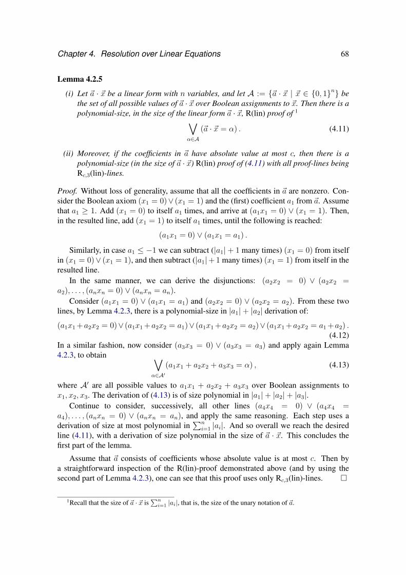
Chapter 4. Resolution over Linear Equations 68
Lemma 4.2.5
(i) Let ~a · ~x be a linear form with n variables, and let A := ~a · ~x | ~x ∈ 0, 1n bethe set of all possible values of ~a · ~x over Boolean assignments to ~x. Then there is apolynomial-size, in the size of the linear form ~a · ~x, R(lin) proof of 1∨
α∈A
(~a · ~x = α) . (4.11)
(ii) Moreover, if the coefficients in ~a have absolute value at most c, then there is apolynomial-size (in the size of ~a · ~x) R(lin) proof of (4.11) with all proof-lines beingRc,3(lin)-lines.
Proof. Without loss of generality, assume that all the coefficients in ~a are nonzero. Con-sider the Boolean axiom (x1 = 0)∨ (x1 = 1) and the (first) coefficient a1 from ~a. Assumethat a1 ≥ 1. Add (x1 = 0) to itself a1 times, and arrive at (a1x1 = 0) ∨ (x1 = 1). Then,in the resulted line, add (x1 = 1) to itself a1 times, until the following is reached:
(a1x1 = 0) ∨ (a1x1 = a1) .
Similarly, in case a1 ≤ −1 we can subtract (|a1|+ 1 many times) (x1 = 0) from itselfin (x1 = 0)∨ (x1 = 1), and then subtract (|a1|+ 1 many times) (x1 = 1) from itself in theresulted line.
In the same manner, we can derive the disjunctions: (a2x2 = 0) ∨ (a2x2 =a2), . . . , (anxn = 0) ∨ (anxn = an).
Consider (a1x1 = 0) ∨ (a1x1 = a1) and (a2x2 = 0) ∨ (a2x2 = a2). From these twolines, by Lemma 4.2.3, there is a polynomial-size in |a1|+ |a2| derivation of:
(a1x1 +a2x2 = 0)∨ (a1x1 +a2x2 = a1)∨ (a1x1 +a2x2 = a2)∨ (a1x1 +a2x2 = a1 +a2) .(4.12)
In a similar fashion, now consider (a3x3 = 0) ∨ (a3x3 = a3) and apply again Lemma4.2.3, to obtain ∨
α∈A′(a1x1 + a2x2 + a3x3 = α) , (4.13)
where A′ are all possible values to a1x1 + a2x2 + a3x3 over Boolean assignments tox1, x2, x3. The derivation of (4.13) is of size polynomial in |a1|+ |a2|+ |a3|.
Continue to consider, successively, all other lines (a4x4 = 0) ∨ (a4x4 =a4), . . . , (anxn = 0) ∨ (anxn = an), and apply the same reasoning. Each step uses aderivation of size at most polynomial in
∑ni=1 |ai|. And so overall we reach the desired
line (4.11), with a derivation of size polynomial in the size of ~a · ~x. This concludes thefirst part of the lemma.
Assume that ~a consists of coefficients whose absolute value is at most c. Then bya straightforward inspection of the R(lin)-proof demonstrated above (and by using thesecond part of Lemma 4.2.3), one can see that this proof uses only Rc,3(lin)-lines.
1Recall that the size of ~a · ~x is∑ni=1 |ai|, that is, the size of the unary notation of ~a.

Chapter 4. Resolution over Linear Equations 69
Lemma 4.2.6 For every n ∈ N, there is a polynomial-size (in n) R0(lin) proof from
(x1 = 1) ∨ · · · ∨ (xn = 1) (4.14)
of(x1 + . . .+ xn = 1) ∨ · · · ∨ (x1 + . . .+ xn = n) . (4.15)
Proof. We show that for every i ∈ [n], there is a polynomial-size (in n) R0(lin) prooffrom (xi = 1) of (x1 + . . . + xn = 1) ∨ · · · ∨ (x1 + . . . + xn = n). This concludes theproof since, by Lemma 4.2.2, we then can derive from (4.14) (with a polynomial-size (inn) R0(lin) proof) the disjunction (4.14) in which each (xi = 1) (for all i ∈ [n]) is replaceby (x1 + . . . + xn = 1) ∨ · · · ∨ (x1 + . . . + xn = n), which is precisely the disjunction(4.15) (note that (4.15) is an R1,1(lin)-line).
Claim: For every i ∈ [n], there is a a polynomial-size (in n) R0(lin) proof from (xi = 1)of (x1 + . . .+ xn = 1) ∨ · · · ∨ (x1 + . . .+ xn = n).
Proof of claim: By Lemma 4.2.5, for every i ∈ [n] there is a polynomial-size (in n) R0(lin)proof (using only the Boolean axioms) of
(x1 + . . .+xi−1 +xi+1 + . . .+xn = 0)∨· · ·∨ (x1 + . . .+xi−1 +xi+1 + . . .+xn = n−1) .(4.16)
Now add successively (xi = 1) to every equation in (4.16) (note that this can be done inR0(lin)). We obtain precisely (x1 + . . .+ xn = 1) ∨ · · · ∨ (x1 + . . .+ xn = n). Claim
Lemma 4.2.7 There is a polynomial-size (in n) R0(lin) proof of (x1 + . . . + xn = 0) ∨(x1 + . . .+ xn = 1) from the collection of disjunctions consisting of (xi = 0) ∨ (xj = 0),for all 1 ≤ i < j ≤ n.
Proof. We use the less formal reasoning by cases and proceed by induction on n. The basecase for n = 1 is immediate from the Boolean axiom (x1 = 0) ∨ (x1 = 1). Assume wealready have a polynomial-size proof of
(x1 + . . .+ xn = 0) ∨ (x1 + . . .+ xn = 1). (4.17)
If xn+1 = 0 we add xn+1 = 0 to both of the equations in (4.17), and reach:
(x1 + . . .+ xn+1 = 0) ∨ (x1 + . . .+ xn+1 = 1). (4.18)
Otherwise, xn+1 = 1, and so we can cut-off (xn+1 = 0) in all the initial disjunctions(xi = 0)∨ (xn+1 = 0), for all 1 ≤ i ≤ n. We thus obtain (x1 = 0), . . . , (xn = 0). Addingtogether (x1 = 0), . . . , (xn = 0) and (xn+1 = 1) we arrive at
(x1 + . . .+ xn+1 = 1) . (4.19)
So overall, either (4.18) holds or (4.19) holds; and so (using Lemma 4.2.2) we arrive atthe disjunction of (4.19) and (4.18), which is precisely (4.18).

Chapter 4. Resolution over Linear Equations 70
4.3 Implicational Completeness of R(lin)In this section we provide a proof of the implicational completeness of R(lin). We shallneed this property in the sequel (see Section 4.4.2). Essentially, a system is implicationallycomplete if whenever something is semantically implied by a set of initial premises, thenit is also derivable from the initial premises. As a consequence, the proof of implicationalcompleteness in this section establishes an alternative completeness proof to that obtainedvia simulating resolution (see Proposition 4.1.4). Note that we are not concerned in thissection with the size of the proofs, but only with their existence.
Formally, we say that R(lin) is implicationally complete if for every collection of dis-junctions of linear equationsD0, D1, . . . , Dm, it holds thatD1, . . . , Dm |= D0 implies thatthere is an R(lin) proof of D0 from D1, . . . , Dm.
Theorem 4.3.1 R(lin) is implicationally complete.
Proof. We proceed by induction on n, the number of variables x1, . . . , xn inD0, D1, . . . , Dm.
The base case n = 0. We need to show that D1, . . . , Dm |= D0 implies that there is anR(lin) proof ofD0 fromD1, . . . , Dm, where allDi’s (for 0 ≤ i ≤ m) have no variables butonly constants. This means that each Di is a disjunction of equations of the form (0 = a0)for some integer a0 (if a linear equation have no variables, then the left hand side of thisequation must be 0; see Section 4.1.1).
There are two cases to consider. In the first case D0 is satisfiable. Since D0 hasno variables, this means precisely that D0 is the equation (0 = 0). Thus, D0 can bederived easily from any axiom in R(lin) (for instance, by subtracting each equation in(x1 = 0) ∨ (x1 = 1) from itself, to reach (0 = 0) ∨ (0 = 0), which is equal to (0 = 0),since we discard duplicate equations inside disjunctions).
In the second case D0 is unsatisfiable. Thus, since D1, . . . , Dm |= D0, there is noassignment satisfying all D1, . . . , Dm. Hence, there must be at least one unsatisfiabledisjunction Di in D1, . . . , Dm (as a disjunction with no variables is either tautologicalor unsatisfiable). Such an unsatisfiable Di is a disjunction of zero or more unsatisfiableequations of the form (0 = a0), for some integer a0 6= 0. We can then use simplificationto cut-off all the unsatisfiable equations in Di to reach the empty disjunction. By theweakening rule, we can now derive D0 from the empty disjunction.
The induction step. Assume that the theorem holds for disjunctions with n variables.Let the underlying variables of D0, D1, . . . , Dm be x1, . . . , xn+1, and assume that
D1, . . . , Dm |= D0 . (4.20)
We write the disjunction D0 as:
t∨j=1
(n∑i=1
a(j)i xi + a
(j)n+1xn+1 = a
(j)0
), (4.21)

Chapter 4. Resolution over Linear Equations 71
where the a(j)i ’s are integer coefficients. We need to show that there is an R(lin) proof of
D0 from D1, . . . , Dm.Let D be a disjunction of linear equations, let xi be a variable and let b ∈ 0, 1. We
shall denote by Dxi=b the disjunction D, where in every equation in D the variable xiis substituted by b, and the constant terms in the left hand sides of all resulting equations(after substituting b for xi) switch sides (and change signs, obviously) to the right handsides of the equations (we have to switch sides of constant terms, as by definition linearequations in R(lin) proofs have all constant terms appearing only on the right hand sidesof equations).
We now reason (slightly) informally inside R(lin) (as illustrated in Section 4.2.1). Fixsome b ∈ 0, 1, and assume that xn+1 = b. Then, fromD1, . . . , Dm we can derive (insideR(lin)):
D1xn+1=b, . . . , Dmxn+1=b . (4.22)
The only variables occurring in (4.22) are x1, . . . , xn. From assumption (4.20) we clearlyhave D1xn+1=b, . . . , Dmxn+1=b |= D0xn+1=b. And so by the induction hypothesis there isan R(lin) derivation of D0xn+1=b from D1xn+1=b, . . . , Dmxn+1=b. So overall, assumingthat xn+1 = b, there is an R(lin) derivation of D0xn+1=b from D1, . . . , Dm.
We now consider the two possible cases: xn+1 = 0 and xn+1 = 1.In case xn+1 = 0, by the above discussion, we can deriveD0xn+1=0 fromD1, . . . , Dm.
For every j ∈ [t], add successively (a(j)n+1 times) the equation xn+1 = 0 to the jth equation
in D0xn+1=0 (see (4.21)). We thus obtain precisely D0.In case xn+1 = 1, again, by the above discussion, we can derive D0 xn+1=1 from
D1, . . . , Dm. For every j ∈ [t], add successively (a(j)n+1 times) the equation xn+1 = 1 to
the jth equation in D0xn+1=1 (recall that we switch sides of constant terms in every linearequation after the substitution of xn+1 by 1 is performed in D0xn+1=1). Again, we obtainprecisely D0.
4.4 Short Proofs for Hard TautologiesIn this section we show that R0(lin) is already enough to admit small proofs for “hard”counting principles like the pigeonhole principle and the Tseitin graph formulas for con-stant degree graphs. On the other hand, as we shall see in Section 4.6, R0(lin) inherits thesame weakness that cutting planes proofs have with respect to the clique-coloring tautolo-gies. Nevertheless, we can efficiently prove the clique-coloring principle in (the strongersystem) R(lin), but not by using R(lin) “ability to count”, rather by using its (straightfor-ward) ability to simulate Res(2) proofs (that is, resolution proofs extended to operate with2-DNF formulas, instead of clauses).

Chapter 4. Resolution over Linear Equations 72
4.4.1 The Pigeonhole Principle Tautologies in R0(lin)
This subsection illustrates polynomial-size R0(lin) proofs of the pigeonhole principle.This will also allow us to establish polynomial-size multilinear proofs operating withdepth-3 multilinear formulas of the pigeonhole principle in the next chapter (Section 5.3).
The m to n pigeonhole principle states that m pigeons cannot be mapped one-to-oneinto n < m holes. As a propositional formula it is usually formulated: ∧
i∈[m]
∨k∈[n]
xi,k
−→ ∨i<j∈[m]
∨k∈[n]
(xi,k ∧ xj,k) , (4.23)
where each propositional variable xi,j designates that the pigeon i is mapped to the holej. It is clear that if m > n then PHPmn is a tautology.
The negation of (4.23), formulated as an unsatisfiable CNF formula, consists of thefollowing clauses:
∀i ∈ [m], xi,1 ∨ . . . ∨ xi,n∀i < j ∈ [m]∀k ∈ [n], ¬xi,k ∨ ¬xj,k (4.24)
This translates (via the translation scheme in Section 4.1.1) into the following unsatisfiablecollection of disjunctions of linear equations, denoted ¬PHPmn :
Definition 4.4.1 The ¬PHPmn is the following set of clauses:
1. Pigeon axioms: (xi,1 = 1) ∨ · · · ∨ (xi,n = 1), for all 1 ≤ i ≤ m;
2. Hole axioms: (xi,k = 0) ∨ (xj,k = 0), for all 1 ≤ i < j ≤ m and for all1 ≤ k ≤ n.
We now describe a polynomial-size in n refutation of ¬PHPmn inside R0(lin). For thispurpose it is sufficient to prove a polynomial-size refutation of the pigeonhole principlewhen the number of pigeons m equals n + 1 (because the set of clauses pertaining to¬PHPn+1
n is already contained in the set of clauses pertaining to ¬PHPmn , for any m > n).Thus, we fixm = n+1. In this subsection we shall say a proof in R0(lin) is of polynomial-size, always intending polynomial-size in n (unless otherwise stated).
By Lemma 4.2.6, for all i ∈ [m] we can derive from the Pigeon axiom (for the ithpigeon):
(xi,1 + . . .+ xi,n = 1) ∨ · · · ∨ (xi,1 + . . .+ xi,n = n) (4.25)
with a polynomial-size R0(lin) proof.By Lemma 4.2.7, from the Hole axioms we can derive, with a polynomial-size R0(lin)
proof(x1,j + . . .+ xm,j = 0) ∨ (x1,j + . . .+ xm,j = 1), (4.26)
for all j ∈ [n].Let S abbreviate the sum of all formal variables xi,j . In other words,
S :=∑
i∈[m],j∈[n]
xi,j .

Chapter 4. Resolution over Linear Equations 73
Lemma 4.4.2 There is a polynomial-size R0(lin) proof from (4.25) (for all i ∈ [m]) of
(S = m) ∨ (S = m+ 1) · · · ∨ (S = m · n).
Proof. For every i ∈ [m] fix the abbreviation zi := xi,1 + . . . + xi,n. Thus, by (4.25) wehave (zi = 1) ∨ · · · ∨ (zi = n).
Consider (z1 = 1)∨ · · · ∨ (z1 = n) and (z2 = 1)∨ · · · ∨ (z2 = n). By Corollary 4.2.4,we can derive from these two lines
(z1 + z2 = 2) ∨ (z1 + z2 = 3) ∨ · · · ∨ (z1 + z2 = 2n) (4.27)
with a polynomial-size R0(lin) proof.Now, consider (z3 = 1) ∨ · · · ∨ (z3 = n) and (4.27). By Corollary 4.2.4 again, from
these two lines we can derive with a polynomial-size R0(lin) proof:
(z1 + z2 + z3 = 3) ∨ (z1 + z2 + z3 = 4) ∨ · · · ∨ (z1 + z2 + z3 = 3n) . (4.28)
Continuing in the same way, we eventually arrive at
(z1 + . . .+ zm = m) ∨ (z1 + . . .+ zm = m+ 1) ∨ · · · ∨ (z1 + . . .+ zm = m · n) ,
which concludes the proof, since S equals z1 + . . .+ zm.
Lemma 4.4.3 There is a polynomial-size R0(lin) proof from (4.26) of
(S = 0) ∨ · · · ∨ (S = n).
Proof. For all j ∈ [n], fix the abbreviation yj := x1,j + . . . + xm,j . Thus, by (4.26) wehave (yj = 0) ∨ (yj = 1), for all j ∈ [n]. Now the proof is similar to the proof of Lemma4.2.5, except that here single variables are abbreviations of linear forms.
If y1 = 0 then we can add y1 to the two sums in (y2 = 0) ∨ (y2 = 1), and reach(y1 + y2 = 0) ∨ (y1 + y2 = 1) and if y1 = 1 we can do the same and reach (y1 + y2 =1) ∨ (y1 + y2 = 2). So, by Lemma 4.2.2, we can derive with a polynomial-size R0(lin)proof
(y1 + y2 = 0) ∨ (y1 + y2 = 1) ∨ (y1 + y2 = 2) . (4.29)
Now, we consider the three cases in (4.29): y1 + y2 = 0 or y1 + y2 = 1 or y1 + y2 = 2,and the clause (y3 = 0) ∨ (y3 = 1). We arrive in a similar manner at (y1 + y2 + y3 =0) ∨ · · · ∨ (y1 + y2 + y3 = 3). We continue in the same way until we arrive at (S =0) ∨ · · · ∨ (S = n).
Theorem 4.4.4 There is a polynomial-size R0(lin) refutation of the m to n pigeonholeprinciple ¬PHPmn .
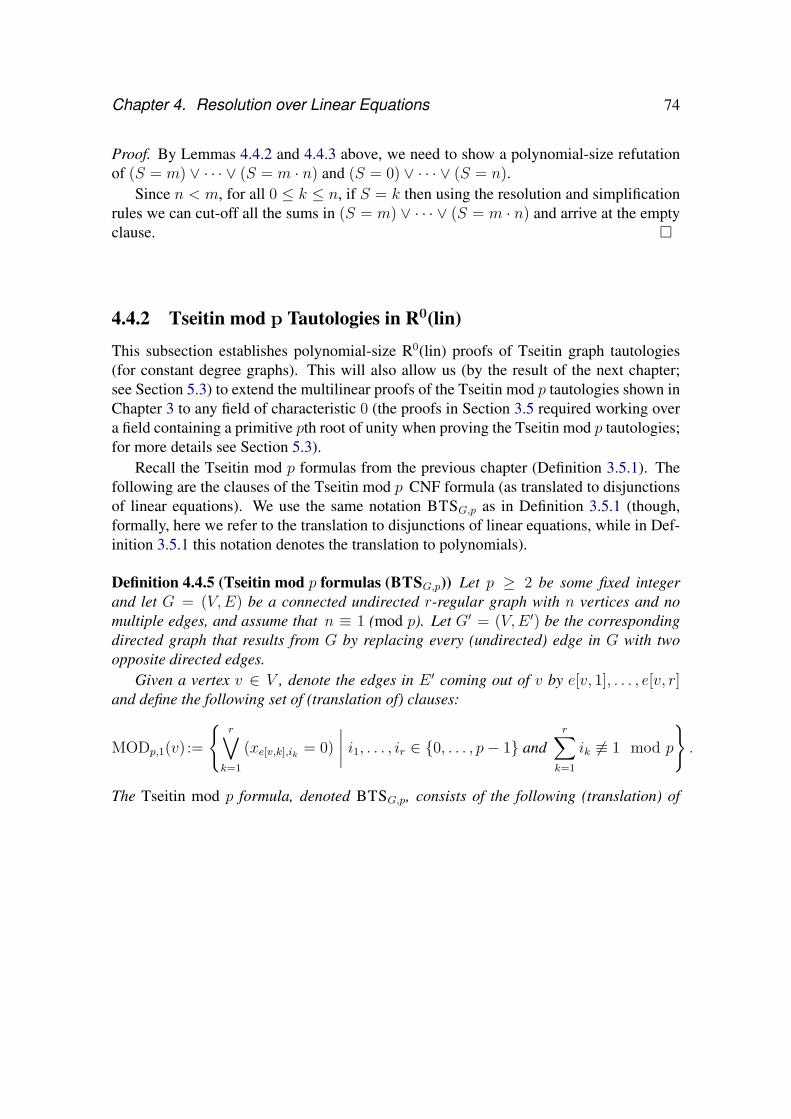
Chapter 4. Resolution over Linear Equations 74
Proof. By Lemmas 4.4.2 and 4.4.3 above, we need to show a polynomial-size refutationof (S = m) ∨ · · · ∨ (S = m · n) and (S = 0) ∨ · · · ∨ (S = n).
Since n < m, for all 0 ≤ k ≤ n, if S = k then using the resolution and simplificationrules we can cut-off all the sums in (S = m) ∨ · · · ∨ (S = m · n) and arrive at the emptyclause.
4.4.2 Tseitin mod p Tautologies in R0(lin)
This subsection establishes polynomial-size R0(lin) proofs of Tseitin graph tautologies(for constant degree graphs). This will also allow us (by the result of the next chapter;see Section 5.3) to extend the multilinear proofs of the Tseitin mod p tautologies shown inChapter 3 to any field of characteristic 0 (the proofs in Section 3.5 required working overa field containing a primitive pth root of unity when proving the Tseitin mod p tautologies;for more details see Section 5.3).
Recall the Tseitin mod p formulas from the previous chapter (Definition 3.5.1). Thefollowing are the clauses of the Tseitin mod p CNF formula (as translated to disjunctionsof linear equations). We use the same notation BTSG,p as in Definition 3.5.1 (though,formally, here we refer to the translation to disjunctions of linear equations, while in Def-inition 3.5.1 this notation denotes the translation to polynomials).
Definition 4.4.5 (Tseitin mod p formulas (BTSG,p)) Let p ≥ 2 be some fixed integerand let G = (V,E) be a connected undirected r-regular graph with n vertices and nomultiple edges, and assume that n ≡ 1 (mod p). Let G′ = (V,E ′) be the correspondingdirected graph that results from G by replacing every (undirected) edge in G with twoopposite directed edges.
Given a vertex v ∈ V , denote the edges in E ′ coming out of v by e[v, 1], . . . , e[v, r]and define the following set of (translation of) clauses:
MODp,1(v) :=
r∨
k=1
(xe[v,k],ik = 0)
∣∣∣∣ i1, . . . , ir ∈ 0, . . . , p− 1 andr∑
k=1
ik 6≡ 1 mod p
.
The Tseitin mod p formula, denoted BTSG,p, consists of the following (translation) of

Chapter 4. Resolution over Linear Equations 75
clauses:
1.p−1∨i=0
(xe,i = 1) , for all e ∈ E ′
(expresses that every edge is assigned at least one value from 0, . . . , p− 1);2. (xe,i = 0) ∨ (xe,j = 0) , for all i 6= j ∈ 0, . . . , p− 1 and all e ∈ E ′(expresses that every edge is assigned at most one value from 0, . . . , p− 1);3. (xe,i = 1) ∨ (xe,p−i = 0) and (xe,i = 0) ∨ (xe,p−i = 1), 2
for all two opposite directed edges e, e ∈ E ′ and all i ∈ 0, . . . , p− 1(expresses condition (i) of the Tseitin mod p principle above);4. MODp,1(v) , for all v ∈ V(expresses condition (ii) of the Tseitin mod p principle above).
Note that for every edge e ∈ E ′, the clauses (1,2) in Definition 4.4.5, combined withthe Boolean axioms of R0(lin), force any collection of edge-variables xe,0, . . . , xe,p−1 tocontain exactly one i ∈ 0, . . . , p− 1 so that xe,i = 1. Also, it is easy to verify that, givena vertex v ∈ V , any assignment σ of 0, 1 values (to the relevant variables) satisfies boththe disjunctions of (1,2) and the disjunctions of MODp,1(v) if and only if σ correspondsto an assignment of values from 0, . . . , p− 1 to the edges coming out of v that sums upto 1 (mod p).
For the rest of this subsection we fix an integer p ≥ 2 and a connected undirected r-regular graph G = (V,E) with n vertices and no multiple edges, such that n ≡ 1 mod pand r is a constant. As in Definition 4.4.5, we let G′ = (V,E ′) be the correspondingdirected graph that results from G by replacing every (undirected) edge in G with twoopposite directed edges. Note that BTSG,p consists of only R1,1(lin)-lines (as translationsof clauses). We now proceed to refute BTSG,p inside R0(lin) with a polynomial-size (inn) refutation.
Given a vertex v ∈ V , and the edges in E ′ coming out of v, denoted e[v, 1], . . . , e[v, r],define the following abbreviation:
αv :=r∑j=1
p−1∑i=0
i · xe[v,j],i . (4.30)
Lemma 4.4.6 There are constants c, d (depending only on r, p), such that for any vertexv ∈ V in G′, there exists a constant-size (also depending only on r, p) R0(lin)-proof fromBTSG,p, containing only Rc,d(lin)-lines, of the following disjunction:
r−1∨`=0
(αv = 1 + ` · p) . (4.31)
2If i = 0 then xe,p−i denotes xe,0.

Chapter 4. Resolution over Linear Equations 76
Proof. Let Tv ⊆ BTSG,p be the set of all disjunctions of the form (1,2,4) from Definition4.4.5 that contain only variables pertaining to vertex v (that is, all the variables xe,i, wheree ∈ E ′ is an edge coming out of v, and i ∈ 0, . . . , p− 1).Claim: Tv semantically implies (4.31), that is:3
Tv |=r−1∨`=0
(αv = 1 + ` · p) .
Proof of claim: Let σ be an assignment of 0, 1 values to the variables in Tv that satisfiesboth the disjunctions of (1,2) and the disjunctions of MODp,1(v) in Definition 4.4.5. Asmentioned above (the comment after Definition 4.4.5), such a σ corresponds to an as-signment of values from 0, . . . , p− 1 to the edges coming out of v that sums up to 1mod p. This means precisely that αv = 1 mod p under the assignment σ. Thus, thereexists a nonnegative integer k, such that αv = 1 + kp under σ.
It remains to show that k ≤ r − 1 (and so the only possible values that αv can getunder σ are 1, 1 + p, 1 + 2p, . . . , 1 + (r − 1)p). Note that because σ gives the value 1 toonly one variable from xe[v,j],0, . . . , xe[v,j],p−1 (for every j ∈ [r]), then the maximal valuethat αv can have under σ is r(p− 1). Thus, 1 + kp ≤ rp− r and so k ≤ r − 1. Claim
From Claim 4.4.2 and from the implicational completeness of R(lin) (Theorem 4.3.1),there exists an R(lin) derivation of (4.31) from Tv. This derivation clearly has size de-pending only on r, p and contains only Rc,d(lin)-lines, where c, d are some two integersthat depend only on r, p.
Lemma 4.4.7 Let c′ = maxc, 2p and d′ = maxd, 3, where c, d are the integers takenfrom Lemma 4.4.6 (note that c′, d′ depend only on r, p). Then there is a polynomial-size(in n) R0(lin) derivation from BTSG,p, containing only Rc′,d′(lin)-lines, of the followingdisjunction:
(r−1)·n∨`=0
(∑v∈V
αv = n+ ` · p).
Proof. Simply add successively all the equations pertaining to disjunctions (4.31), for allvertices v ∈ V . Formally, we show that for every subset of vertices V ⊆ V , with |V| = k,there is a polynomial-size (in n) R(lin) derivation from BTSG,p of
(r−1)·k∨`=0
(∑v∈V
αv = k + ` · p), (4.32)
containing only Rc′,d′(lin)-lines. Thus, putting V = V , will conclude the proof
3Recall that we only consider assignments of 0, 1 values to variables when considering the semanticimplication relation |=.

Chapter 4. Resolution over Linear Equations 77
We proceed by induction on the size of V . The base case, |V| = 1, is immediate fromLemma 4.4.6.
Assume that we already derived (4.32) with a polynomial-size (in n) R(lin) proof con-taining only Rc′,d′(lin)-lines, for some V ⊂ V , such that |V| = k < n. Let u ∈ V \ V . ByLemma 4.4.6, we can derive
r−1∨`=0
(αu = 1 + ` · p) (4.33)
from BTSG,p with a constant-size proof that contains only Rc,d(lin)-lines.Note that both (4.32) and (4.33) are R2p,1(lin)-lines. Thus, by Lemma 4.2.3, each linear
equation in (4.33) can be added to each linear equation in (4.32), with a polynomial-size (in n) R(lin) proof that contains only R2p,3(lin)-lines. This results in the followingdisjunction:
(r−1)·(k+1)∨`=0
∑v∈V∪u
αv = k + 1 + ` · p
,
which is precisely what we need to conclude the induction step.
Given a pair of opposite directed edges e, e in G′, denote by Te ⊆ BTSG,p the setof all disjunctions of the form (1,2,3) from Definition 4.4.5 that contain only variablespertaining to edges e, e (that is, all the variables xe,j, xe,j , for all j ∈ 0, . . . , p− 1).Lemma 4.4.8 There are two integers c′′, d′′ that depend only on r, p, such that for any pairof opposite directed edges e, e in G′ and any i ∈ 0, . . . , p− 1, there exists a constant-size (depending only on r, p) R0(lin) proof, containing only Rc′′,d′′(lin)-lines, from Te of thefollowing disjunction:
(i · xe,i + (p− i) · xe,p−i = 0) ∨ (i · xe,i + (p− i) · xe,p−i = p) . (4.34)
Proof. First note that Te semantically implies
(xe,i + xe,p−i = 0) ∨ (xe,i + xe,p−i = 2) . (4.35)
The number of variables in Te and (4.35) is constant. Hence, there is a constant-sizeR0(lin)-proof of (4.34) from Te. Also note that
(xe,i + xe,p−i = 0) ∨ (xe,i + xe,p−i = 2) |=(i · xe,i + (p− i) · xe,p−i = 0) ∨ (i · xe,i + (p− i) · xe,p−i = p) .
(4.36)Therefore, there is also an R0(lin)-proof of constant-size from Te of the lower line in (4.36)that uses only Rc′′,d′′(lin)-lines, for some two integers c′′, d′′ depending only on r, p.
We are now ready to complete the polynomial-size R0(lin) refutation of BTSG,p. Usingthe two prior lemmas, the refutation idea is simple, as we now explain. Observe that∑
v∈V
αv =∑e,e⊆E′
i∈0,...,p−1
(i · xe,i + (p− i) · xe,p−i) , (4.37)

Chapter 4. Resolution over Linear Equations 78
where by e, e ⊆ E ′ we mean that e, e is a pair of opposite directed edges in G′.Derive by Lemma 4.4.7 the disjunction
(r−1)·n∨`=0
(∑v∈V
αv = n+ ` · p). (4.38)
This disjunction expresses the fact that∑
v∈V αv = 1 mod p (since n = 1 mod p). Onthe other hand, using Lemma 4.4.8, we can “sum together” all the equations (4.34) (for alle, e ⊆ E ′ and all i ∈ 0, . . . , p− 1), to obtain a disjunction expressing the statementthat ∑
e,e⊆E′i∈0,...,p−1
(i · xe,i + (p− i) · xe,p−i) = 0 mod p .
By Equation (4.37), we then obtain the desired contradiction. This idea is formalized inthe proof of the following theorem:
Theorem 4.4.9 Let G = (V,E) be an r-regular graph with n vertices, where r is a con-stant. Fix some modulus p. Then, there are polynomial-size (in n) R0(lin) refutations ofBTSG,p.
Proof. Let s, t be two integers (depending only on r, p) defined as s = maxc′, c′′ andt = maxd′, d′′, where c′, d′ are taken from Lemma 4.4.7 and c′′, d′′ are taken fromLemma 4.4.8.
First, use Lemma 4.4.7 to derive
(r−1)·n∨`=0
(∑v∈V
αv = n+ ` · p), (4.39)
using only Rs,t(lin)-lines. Second, use Lemma 4.4.8 to derive
(i · xe,i + (p− i) · xe,p−i = p) ∨ (i · xe,i + (p− i) · xe,p−i = 0) , (4.40)
for every pair of opposite directed edges in G′ = (V,E ′) (as in Definition 4.4.5) and everyresidue i ∈ 0, . . . , p− 1, and using only Rs,t(lin)-lines.
We now reason inside R0(lin). Pick a pair of opposite directed edges e, e and a residuei ∈ 0, . . . , p− 1. If i ·xe,i + (p− i) ·xe,p−i = 0, then subtract this equation successivelyfrom every equation in (4.39). We thus obtain a new disjunction, similar to that of (4.39),but which does not contain the xe,i and xe,p−i variables, and with the same free-terms.
Otherwise, i · xe,i + (p− i) · xe,p−i = p, then subtract this equation successively fromevery equation in (4.39). Again, we obtain a new disjunction, similar to that of (4.39),but which does not contain the xe,i and xe,p−i variables, and such that p is subtracted fromevery free-term in every equation. Since, by assumption, n ≡ 1 mod p, the free-terms inevery equation are (still) equal 1 mod p.

Chapter 4. Resolution over Linear Equations 79
Now, note that (4.39) is an R2p,1(lin)-line, and (4.40) is an Rp,1(lin)-line, and thus thereasoning by (two) cases (that is, i ·xe,i+(p−i) ·xe,p−i = 0 and i ·xe,i+(p−i) ·xe,p−i = p)as demonstrated above can be done in R0(lin) using only Rs′,t′(lin)-lines, where s′, t′ aretwo integers depending only on p (these s′, t′ come from using the reasoning-by-caseswhich implicitly uses Lemma 4.2.2).
So overall, we applied a polynomial-size R0(lin)-proofs, containing only Rs′,t′(lin)-lines, and reached a new R2p,1(lin)-line, in which all the free-terms in the equations equal1 mod p.
We now continue the same process for every pair e, e of opposite directed edges inG′ and every residue i. Since in each such step we start from an R2p,1(lin)-line and anRp,1(lin)-line (as demonstrated above), then this process can be carried over in R0(lin) (asdemonstrated above, we only use Rs′′,t′′(lin)-lines in this process, for s′′ = maxs, s′ andt′′ = maxt, t′).
Eventually, we discard all the variables xe,i in the equations, for every e ∈ E ′ andi ∈ 0, . . . , p− 1, while all the free-terms in every equation remain to be equal 1 mod p.Therefore, we arrive at a disjunction of equations of the form (0 = γ) for some γ = 1mod p. By using the simplification rule we can cut-off all such equations, and arrivefinally at the empty disjunction.
4.4.3 The Clique-Coloring Principle in R(lin)
In this section we observe that there are polynomial-size R(lin) proofs of the clique-coloring principle (for certain weak parameters). This implies in particular that R(lin)does not possess the feasible monotone interpolation property (see more details on theinterpolation method in Section 4.5).
Atserias, Bonet and Esteban (Atserias et al. (2002)) demonstrated polynomial-sizeRes(2) refutations of the clique-coloring formulas (for certain weak parameters; see Theo-rem 4.4.13 below). Thus, it is sufficient to show that R(lin) polynomially-simulates Res(2)proofs (Proposition 4.4.12). This can be shown in a straightforward manner. As noted inthe first paragraph of Section 4.4, because the proofs of the clique-coloring formula wediscuss here only follow the proofs inside Res(2), then in fact these proofs do not takeany advantage of the capability to “count” inside R(lin) (this capability is exemplified, forinstance, in Section 4.2.2).
We start with the clique-coloring formulas (these formulas will also be used in Section4.6). These formulas express the clique-coloring principle that has been widely used inthe proof complexity literature (cf., Bonet et al. (1997), Pudlak (1997), Krajıcek (1997),Krajıcek (1998), Atserias et al. (2002), Krajıcek (2007)). This principle is based on thefollowing basic combinatorial idea. LetG = (V,E) be an undirected graph with n verticesand let k′ < k be two integers. Then, one of the following must hold:
(i) The graph G does not contain a clique with k vertices;

Chapter 4. Resolution over Linear Equations 80
(ii) The graph G is not a complete k′-partite graph. In other words, there is no way topartition G into k′ subgraphs G1, . . . , Gk′ , such that every Gi is an independent set,and for all i 6= j ∈ [k′], all the vertices in Gi are connected by edges (in E) to allthe vertices in Gj .
Obviously, if Item (ii) above is false (that is, if G is a complete k′-partite graph), thenthere exists a k′-coloring of the vertices of G; hence the name clique-coloring for theprinciple.
The propositional formulation of the (negation of the) clique-coloring principle is asfollows. Each variable pi,j , for all i 6= j ∈ [n], is an indicator variable for the fact thatthere is an edge in G between vertex i and vertex j. Each variable q`,i, for all ` ∈ [k] andall i ∈ [n], is an indicator variable for the fact that the vertex i in G is the `th vertex in thek-clique. Each variable r`,i, for all ` ∈ [k′] and all i ∈ [n], is an indicator variable for thefact that the vertex i in G is in the independent set G`.
Definition 4.4.10 (The Clique-Coloring formulas) The negation of the clique-coloringprinciple consists of the following unsatisfiable collection of clauses (as translated to dis-junctions of linear equations), denoted ¬CLIQUEnk,k′:
i. (q`,1 = 1) ∨ · · · ∨ (q`,n = 1), for all ` ∈ [k]
(expresses that there exists at least one vertex in G which constitutes the `th vertexof the k-clique);
ii. (q`,i = 0) ∨ (q`,j = 0), for all i 6= j ∈ [n], ` ∈ [k]
(expresses that there exists at most one vertex in G which constitutes the `th vertexof the k-clique);
iii. (q`,i = 0) ∨ (q`′,i = 0), for all i ∈ [n], ` 6= `′ ∈ [k]
(expresses that the ith vertex of G cannot be both the `th and the `′th vertex of thek-clique);
iv. (q`,i = 0) ∨ (q`′,j = 0) ∨ (pi,j = 1), for all ` 6= `′ ∈ [k], i 6= j ∈ [n]
(expresses that if both the vertices i and j in G are in the k-clique, then there is anedge in G between i and j);
v. (r1,i = 1) ∨ · · · ∨ (rk′,i = 1), for all i ∈ [n]
(expresses that every vertex of G is in at least one independent set);
vi. (r`,i = 0) ∨ (r`′,i = 0), for all ` 6= ` ∈ [k′], i ∈ [n]
(expresses that every vertex of G pertains to at most one independent set);
vii. (pi,j = 0) ∨ (rt,i = 0) ∨ (rt,j = 0), for all i 6= j ∈ [n], t ∈ [k′]
(expresses that if there is an edge between vertex i and j in G, then i and j cannotbe in the same independent set);

Chapter 4. Resolution over Linear Equations 81
Remark: Our formulation of the clique-coloring formulas above is similar to the one usedby Bonet et al. (1997), except that we consider also the pi,j variables (we added the (iv)clauses and changed accordingly the (vii) clauses). This is done for the sake of clarity ofthe contradiction itself, and also to make it clear that the formulas are in the appropriateform required by the interpolation method (see Section 4.5 for details on the interpolationmethod). By resolving over the pi,j variables in (iv) and (vii), one can obtain precisely thecollection of clauses in Bonet et al. (1997).
Atserias, Bonet and Esteban (Atserias et al. (2002)) demonstrated polynomial-size (inn) Res(2) refutations of ¬CLIQUEnk,k′ , when k =
√n and k′ = (log n)2/8 log log n. These
are rather weak parameters, but they suffice to establish the fact that Res(2) does notpossess the feasible monotone interpolation property.
The Res(2) proof system (also called 2-DNF resolution), first considered in Krajıcek(2001), is resolution extended to operate with 2-DNF formulas, defined as follows.
A 2-term is a conjunction of up to two literals. A 2-DNF is a disjunction of 2-terms.The size of a 2-term is the number of literals in it (that is, either 1 or 2). The size of a2-DNF is the total size of all the 2-terms in it.
Definition 4.4.11 (Res(2)) A Res(2) proof of a 2-DNF D from a collection K of 2-DNFsis a sequence of 2-DNFs D1, D2, . . . , Ds , such that Ds = D, and every Dj is either fromK or was derived from previous line(s) in the sequence by the following inference rules:
Cut Let A,B be two 2-DNFs.
From A∨∧2i=1 li and B∨∨2
i=1 ¬li derive A∨B, where the li’s are (not necessarilydistinct) literals (and ¬li is the negation of the literal li).
AND-introduction Let A,B be two 2-DNFs and l1, l2 two literals.
From A ∨ l1 and B ∨ l2 derive A ∨B ∨∧2i=1 li.
Weakening From a 2-DNF A derive A ∨ ∧2i=1 li , where the li’s are (not necessarily
distinct) literals.
A Res(2) refutation of a collection of 2-DNFs K is a Res(2) proof of the empty disjunction from K (the empty disjunction stands for FALSE). The size of a Res(2) proof is the totalsize of all the 2-DNFs in it.
Given a collection K of 2-DNFs we translate it into a collection of disjunctions oflinear equations via the following translation scheme. For a literal l, denote by l thetranslation that maps a variable xi into xi, and ¬xi into 1 − xi. A 2-term l1 ∧ l2 is firsttransformed into the equation l1 + l2 = 2, and then changing sides of the free-terms so thatthe final translation of l1 ∧ l2 has only a single free-term in the right hand side. A disjunc-tion of 2-terms (that is, a 2-DNF) D =
∨i∈I(li,1 ∧ li,2) is translated into the disjunction of
the translations of the 2-terms, denoted by D. It is clear that every assignment satisfies a2-DNF D if and only if it satisfies D.

Chapter 4. Resolution over Linear Equations 82
Proposition 4.4.12 R(lin) polynomially simulates Res(2). In other words, if π is a Res(2)proof of D from a collection of 2-DNFs K1, . . . , Kt, then there is an R(lin) proof of Dfrom K1, . . . , Kt whose size is polynomial in the size of π.
The proof of Proposition 4.4.12 proceeds by induction on the length (that is, the num-ber of proof-lines) in the Res(2) proof. This is pretty straightforward and similar to thesimulation of resolution by R(lin), as illustrated in the proof of Proposition 4.1.4. We omitthe details.
Theorem 4.4.13 (Atserias et al. (2002)) Let k =√n and k′ = (log n)2/8 log log n.
Then ¬CLIQUEnk,k′ has Res(2) refutations of size polynomial in n.
Thus, Proposition 4.4.12 yields the following:
Corollary 4.4.14 Let k, k′ be as in Theorem 4.4.13. Then ¬CLIQUEnk,k′ has R(lin) refuta-tions of size polynomial in n.
The following corollary is important (we refer the reader to Section 4.5.3 for the nec-essary relevant definitions concerning the feasible monotone interpolation property).
Corollary 4.4.15 R(lin) does not possess the feasible monotone interpolation property.
Remark: The proof of ¬CLIQUEnk,k′ inside Res(2) demonstrated in Atserias et al. (2002)(and hence, also the corresponding proof inside R(lin)) proceeds along the following lines.First reduce ¬CLIQUEnk,k′ to the k to k′ pigeonhole principle. For the appropriate valuesof the parameters k and k′ — and specifically, for the values in Theorem 4.4.13 — thereis a short resolution proof of the k to k′ pigeonhole principle (this was shown in Buss andPitassi (1997)); (this resolution proof is polynomial in the number of pigeons k, but notin the number of holes k′, which is exponentially smaller than k).4 Therefore, in order toconclude the refutation of ¬CLIQUEnk,k′ inside Res(2) (or inside R(lin)), it suffices to sim-ulate the short resolution refutation of the k to k′ pigeonhole principle. It is importantto emphasize this point: After reducing, inside R(lin), ¬CLIQUEnk,k′ to the pigeonholeprinciple, one simulates the resolution refutation of the pigeonhole principle, and this hasnothing to do with the small-size R0(lin) refutations of the pigeonhole principle demon-strated in Section 4.4.1. This is because, the reduction (inside R(lin)) of ¬CLIQUEnk,k′to the k to k′ pigeonhole principle, results in a substitution instance of the pigeonholeprinciple formulas; in other words, the reduction results in a collection of disjunctionsthat are similar to the pigeonhole principle disjunctions where each original pigeonholeprinciple variable is substituted by some big formula (and, in particular, there are no twointegers c, d independent from the number of variables, such that these disjunctions areall Rc,d(lin)-lines). (Note that R0(lin) does not admit short proofs of the clique-coloringformulas as we show in Section 4.6.)
4Whenever k ≥ 2k′ the k to k′ pigeonhole principle is referred to as the weak pigeonhole principle.

Chapter 4. Resolution over Linear Equations 83
4.5 Interpolation Results for R0(lin)In this section we study the applicability of the feasible (non-monotone) interpolationtechnique to R0(lin) refutations. In particular, we show that R0(lin) admits a polyno-mial (in terms of the R0(lin)-proofs) upper bound on the (non-monotone) circuit-size ofinterpolants. In the next section we shall give a polynomial upper bound on the mono-tone circuit-size of interpolants, but only in the case that the interpolant corresponds tothe clique-coloring formulas (whereas, in this section we are interested in the generalcase; that is, upper bounding circuit-size of interpolants corresponding to any formula[of the prescribed type; see below]). First, we shortly describe the feasible interpolationmethod and explain how this method can be applied to obtain (sometime, conditional)lower bounds on proof size. Explicit usage of the interpolation method in proof complex-ity goes back to Krajıcek (1994).
Let Ai(~p, ~q), i ∈ I , and Bj(~p, ~r), j ∈ J , (I and J are sets of indices) be a collectionof formulas (for instance, a collection of disjunctions of linear equations) in the displayedvariables only. Denote byA(~p, ~q) the conjunction of allAi(~p, ~q), i ∈ I , and byB(~p, ~r), theconjunction of all Bj(~p, ~r), j ∈ J . Assume that ~p, ~q, ~r are pairwise disjoint sets of distinctvariables, and that there is no assignment that satisfies both A(~p, ~q) and B(~p, ~r). Fix anassignment ~α to the variables in ~p. The ~p variables are the only common variables of theAi’s and the Bj’s. Therefore, either A(~α, ~q) is unsatisfiable or B(~α,~r) is unsatisfiable.
The interpolation technique transforms a refutation of A(~p, ~q)∧B(~p, ~r), in some proofsystem, into a circuit (usually a Boolean circuit) that outputs 1 for those assignments ~α(for ~p) for which A(~α, ~q) is unsatisfiable, and outputs 0 for those assignments ~α for whichB(~α,~r) is unsatisfiable (the two cases are not necessarily exclusive, so if both cases holdfor an assignment, the circuit can output either that the first case holds or that the secondcase holds). In other words, given a refutation of A(~p, ~q) ∧B(~p, ~r), we construct a circuitC(~p), called the interpolant, such that
C(~α) = 1 =⇒ A(~α, ~q) is unsatisfiable, andC(~α) = 0 =⇒ B(~α,~r) is unsatisfiable.
(4.41)
(Note that if U denotes the set of those assignments ~α for which A(~α, ~q) is satisfiable, andV denotes the set of those assignments ~α for which B(~α,~r) is satisfiable, then U and Vare disjoint [since A(~p, ~q) ∧ B(~p, ~r) is unsatisfiable], and C(~p) separates U from V ; seeDefinition 4.5.2 below.)
Assume that for a proof system P the transformation from refutations ofA(~p, ~q), B(~p, ~r) into the corresponding interpolant circuit C(~p) results in a circuit whosesize is polynomial in the size of the refutation. Then, an exponential lower bound oncircuits for which (4.41) holds, implies an exponential lower bound on P-refutations ofA(~p, ~q), B(~p, ~r).
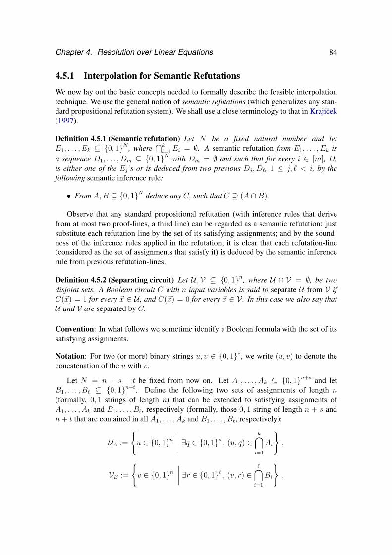
Chapter 4. Resolution over Linear Equations 84
4.5.1 Interpolation for Semantic Refutations
We now lay out the basic concepts needed to formally describe the feasible interpolationtechnique. We use the general notion of semantic refutations (which generalizes any stan-dard propositional refutation system). We shall use a close terminology to that in Krajıcek(1997).
Definition 4.5.1 (Semantic refutation) Let N be a fixed natural number and letE1, . . . , Ek ⊆ 0, 1N , where
⋂ki=1 Ei = ∅. A semantic refutation from E1, . . . , Ek is
a sequence D1, . . . , Dm ⊆ 0, 1N with Dm = ∅ and such that for every i ∈ [m], Di
is either one of the Ej’s or is deduced from two previous Dj, D`, 1 ≤ j, ` < i, by thefollowing semantic inference rule:
• From A,B ⊆ 0, 1N deduce any C, such that C ⊇ (A ∩B).
Observe that any standard propositional refutation (with inference rules that derivefrom at most two proof-lines, a third line) can be regarded as a semantic refutation: justsubstitute each refutation-line by the set of its satisfying assignments; and by the sound-ness of the inference rules applied in the refutation, it is clear that each refutation-line(considered as the set of assignments that satisfy it) is deduced by the semantic inferencerule from previous refutation-lines.
Definition 4.5.2 (Separating circuit) Let U ,V ⊆ 0, 1n, where U ∩ V = ∅, be twodisjoint sets. A Boolean circuit C with n input variables is said to separate U from V ifC(~x) = 1 for every ~x ∈ U , and C(~x) = 0 for every ~x ∈ V . In this case we also say thatU and V are separated by C.
Convention: In what follows we sometime identify a Boolean formula with the set of itssatisfying assignments.
Notation: For two (or more) binary strings u, v ∈ 0, 1∗, we write (u, v) to denote theconcatenation of the u with v.
Let N = n + s + t be fixed from now on. Let A1, . . . , Ak ⊆ 0, 1n+s and letB1, . . . , B` ⊆ 0, 1n+t. Define the following two sets of assignments of length n(formally, 0, 1 strings of length n) that can be extended to satisfying assignments ofA1, . . . , Ak and B1, . . . , B`, respectively (formally, those 0, 1 string of length n + s andn+ t that are contained in all A1, . . . , Ak and B1, . . . , B`, respectively):
UA :=
u ∈ 0, 1n
∣∣∣∣ ∃q ∈ 0, 1s , (u, q) ∈k⋂i=1
Ai
,
VB :=
v ∈ 0, 1n
∣∣∣∣ ∃r ∈ 0, 1t , (v, r) ∈⋂i=1
Bi
.

Chapter 4. Resolution over Linear Equations 85
Definition 4.5.3 (Polynomial upper bounds on interpolants) Let P be a propositionalrefutation system. Assume that ~p, ~q, ~r are pairwise disjoint sets of distinct variables, where~p has n variables, ~q has s variables and ~r has t variables. Let A1(~p, ~q), . . . , Ak(~p, ~q) andB1(~p, ~r), . . . , B`(~p, ~r) be two collections of formulas with the displayed variables only.Assume that for any such A1(~p, ~q), . . . , Ak(~p, ~q) and B1(~p, ~r), . . . , B`(~p, ~r), if there existsa P-refutation of size S for A1(~p, ~q)∧ · · · ∧Ak(~p, ~q)∧B1(~p, ~r)∧ . . .∧B`(~p, ~r) then thereexists a Boolean circuit separating UA from VB of size polynomial in S.5 In this case wesay that P has a polynomial upper bound on interpolant circuits.
4.5.1.1 The Communication Game Technique
The feasible interpolation via communication game technique is based on transformingproofs into Boolean circuits, where the size of the resulting circuit depends on the com-munication complexity of each proof-line. This technique goes back to Impagliazzo et al.(1994) and Razborov (1995) and was subsequently applied and extended in Bonet et al.(1997) and Krajıcek (1997) (Impagliazzo et al. (1994) and Bonet et al. (1997) did not useexplicitly the notion of interpolation of tautologies or contradictions). We shall employ theinterpolation theorem of Krajıcek in Krajıcek (1997) that demonstrates how to transforma small semantic refutation with each proof-line having low communication complexityinto a small Boolean circuit separating the corresponding sets.
The underlying idea of the interpolation via communication game technique is that a(semantic) refutation, where each proof-line is of small (that is, logarithmic) communi-cation complexity, can be transformed into an efficient communication protocol for theKarchmer-Wigderson game (following Karchmer and Wigderson (1988)) for two players.In the Karchmer-Wigderson game the first player knows some binary string u ∈ U andthe second player knows some different binary string v ∈ V , where U and V are disjointsets of strings. The two players communicate by sending information bits to one another(following a protocol previously agreed on). The goal of the game is for the two players todecide on an index i such that the ith bit of u is different from the ith bit of v. An efficientKarchmer-Wigderson protocol (by which we mean a protocol that requires the players toexchange at most a logarithmic number of bits in the worst-case) can then be transformedinto a small circuit separating U from V (see Definition 4.5.2). This efficient transfor-mation from protocols for Karchmer-Wigderson games (described in a certain way) intocircuits, was demonstrated by Razborov in Razborov (1995). So overall, given a seman-tic refutation with proof-lines of low communication complexity, one can obtain a smallcircuit for separating the corresponding sets.
First, we need to define the concept of communication complexity in a suitable way forthe interpolation theorem.
Definition 4.5.4 (Communication complexity; Krajıcek (1997), Definition 4.3) LetN = n + s + t and A ⊆ 0, 1N . Let u, v ∈ 0, 1n, qu ∈ 0, 1s, rv ∈ 0, 1t. Denote
5Here UA and VB are defined as above, by identifying the Ai(~p, ~q)’s and the Bi(~p, ~r)’s with the sets ofassignments that satisfy them.

Chapter 4. Resolution over Linear Equations 86
by ui, vi the ith bit of u, v, respectively, and let (u, qu, rv) and (v, qu, rv) denote theconcatenation of strings u, qu, rv and v, qu, rv, respectively. Consider the following threetasks:
1. Decide whether (u, qu, rv) ∈ A;
2. Decide whether (v, qu, rv) ∈ A;
3. If one of the following holds:
(i) (u, qu, rv) ∈ A and (v, qu, rv) 6∈ A; or
(ii) (u, qu, rv) 6∈ A and (v, qu, rv) ∈ A,
then find an i ∈ [n], such that ui 6= vi;
Consider a game between two players, Player I and Player II, where Player I knowsu ∈ 0, 1n , qu ∈ 0, 1s and Player II knows v ∈ 0, 1n , rv ∈ 0, 1t. The two playerscommunicate by exchanging bits of information between them (following a protocol pre-viously agreed on). The communication complexity of A, denoted CC(A), is the minimal(over all protocols) number of bits that players I and II need to exchange in the worst-casein solving each of Tasks 1, 2 and 3 above.6
For A ⊆ 0, 1n+s define
A :=
(a, b, c)∣∣ (a, b) ∈ A and c ∈ 0, 1t
,
where a and b range over 0, 1n and 0, 1s, respectively. Similarly, for B ⊆ 0, 1n+t
defineB :=
(a, b, c)
∣∣ (a, c) ∈ B and b ∈ 0, 1t,
where a and c range over 0, 1n and 0, 1t, respectively.
Theorem 4.5.5 (Krajıcek (1997), Theorem 5.1) Let A1, . . . , Ak ⊆ 0, 1n+s andB1, . . . , B` ⊆ 0, 1n+t. Let D1, . . . , Dm be a semantic refutation from A1, . . . , Ak andB1, . . . , B`. Assume that CC(Di) ≤ ζ , for all i ∈ [m]. Then, the sets UA and VB (asdefined above) can be separated by a Boolean circuit of size (m+ n)2O(ζ).
4.5.2 Polynomial Upper Bounds on Interpolants for R0(lin)
Here we apply Theorem 4.5.5 to show that R0(lin) has polynomial upper bounds on itsinterpolant circuits. Again, in what follows we sometime identify a disjunction of linearequations with the set of its satisfying assignments.
6In other words, CC(A) is the minimal number ζ, for which there exists a protocol, such that for everyinput (u, qu to Player I and v, rv to Player II) and every task (from Tasks 1, 2 and 3), the players need toexchange at most ζ bits in order to solve the task.

Chapter 4. Resolution over Linear Equations 87
Theorem 4.5.6 R0(lin) has a polynomial upper bound on interpolant circuits (Definition4.5.3).
In light of Theorem 4.5.5, to demonstrate that a certain propositional refutation systemP possesses a polynomial upper bound on interpolant circuits (see Definition 4.5.3) itsuffices to show that any proof-line of P induces a set of assignments with at most alogarithmic (in the number of variables) communication complexity (Definition 4.5.4).Therefore, all we need in order to establish Theorem 4.5.6 is the following lemma:
Lemma 4.5.7 Let k, d be two constants, let D be an Rk,d(lin)-line with N variables, andlet D be the set of assignments that satisfy D. Then, CC(D) = O(logN).
Proof. Let N = n + s + t (and so D ∈ 0, 1n+s+t). For the sake of convenience weshall assume that the N variables in D are partitioned into (pairwise disjoint) three groups~p := (p1 . . . , pn), ~q := (q1, . . . , qs) and ~r := (r1, . . . , rt). Let u, v ∈ 0, 1n, qu ∈ 0, 1s,rv ∈ 0, 1t. Assume that Player I knows u, qu and Player II knows v, rv.
By assumption, we can partition the disjunction D into a constant number d of dis-juncts, where one disjunct is a (possibly empty, translation of a) clause in the ~p, ~q, ~r vari-ables (see Section 4.1.1), and all other disjuncts have the following form:∨
i∈I
(~a · ~p+~b · ~q + ~c · ~r = `i
), (4.42)
where I is (an unbounded) set of indices, `i are integer numbers, for all i ∈ I , and ~a,~b,~cdenote vectors of n, s and t constant coefficients (that is, all the coefficients have an abso-lute value at most k), respectively.
Let us denote the (translation of the) clause from D in the ~p, ~q, ~r variables by
P ∨Q ∨R ,where P ,Q andR denote the (translated) sub-clauses consisting of the ~p, ~q and ~r variables,respectively.
We need to show that by exchangingO(logN) bits, the players can solve each of Tasks1, 2 and 3 from Definition 4.5.4, correctly.
Task 1: The players need to decide whether (u, qu, rv) ∈ D. Player II, who knows rv,computes the numbers ~c · rv, for every ~c pertaining to every disjunct of the form shown inEquation (4.42) above. Then, Player II sends the (binary representation of) these numbersto Player I. Since there are only a constantly many such numbers and the coefficients inevery ~c are also constants, this amounts to O(log t) ≤ O(logN) bits that Player II sendsto Player I. Player II also computes the truth value of the sub-clause R, and sends this(single-bit) value to Player I.
Now, it is easy to see that Player I has sufficient data to compute by herself/himselfwhether (u, qu, rv) ∈ D (Player I can then send a single bit informing Player II whether(u, qu, rv) ∈ D).

Chapter 4. Resolution over Linear Equations 88
Task 2: This is analogous to Task 1.
Task 3: Assume that (u, qu, rv) ∈ D and (v, qu, rv) 6∈ D (the case (u, qu, rv) 6∈ D and(v, qu, rv) ∈ D is analogous).
The first rounds of the protocol are completely similar to that described in Task 1above: Player II, who knows rv, computes the numbers ~c · rv, for every ~c pertainingto every disjunct of the form shown in Equation (4.42) above. Then, Player II sends the(binary representation of) these numbers to Player I. Player II also computes the truth valueof the sub-clause R, and sends this (single-bit) value to Player I. Again, this amounts toO(logN) bits that Player II sends to Player I.
By assumption (that (u, qu, rv) ∈ D and (v, qu, rv) 6∈ D) the players need to deal onlywith the following two cases:
Case 1: The assignment (u, qu, rv) satisfies the clause P ∨ Q ∨ R while (v, qu, rv)falsifies P ∨Q ∨ R. Thus, it must be that ~u satisfies the sub-clause P while ~v falsifies P .This means that for any i ∈ [n] such that ui sets to 1 a literal in P (there ought to existat least one such i), it must be that ui 6= vi. Therefore, all that Player I needs to do is tosend the (binary representation of) index i to Player II. (This amounts to O(logN) bitsthat Player I sends to Player II.)
Case 2: There is some linear equation
~a · ~p+~b · ~q + ~c · ~r = ` (4.43)
in D, such that ~a · u+~b · qu +~c · rv = `. Note that (by assumption that (v, qu, rv) 6∈ D) itmust also hold that: ~a · v+~b · qu +~c · rv 6= ` (and so there is an i ∈ [n], such that ui 6= vi).Player I can find linear equation (4.43), as he/she already received from Player II all thepossible values of ~c · ~r (for all possible ~c ’s in D).
Recall that the left hand side of a linear equation ~d · ~x = ` is called the linear formof the equation. By assumption, there are only constant d many distinct linear forms inD. Since both players know these linear forms, we can assume that each linear form hassome index associated to it by both players. Player I sends to Player II the index of thelinear form ~a · ~p+~b · ~q+~c ·~r from (4.43) in D. Since there are only constantly many suchlinear forms in D, it takes only constant number of bits to send this index.
Now both players need to apply a protocol for finding an i ∈ [n] such that ui 6= vi,where ~a · ~u +~b · qu + ~c · rv = ` and ~a · ~v +~b · qu + ~c · rv 6= `. Thus, it remains only toprove the following claim:
Claim: There is a communication protocol in which Player I and Player II need at mostO(logN) bits of communication in order to find an i ∈ [n] such that ui 6= vi (under theabove conditions).
Proof of claim: We invoke the well-known connection between Boolean circuit-depth andcommunication complexity. Let f : 0, 1N → 0, 1 be a Boolean function. Denote bydp(f) the minimal depth of a bounded fan-in Boolean circuit computing f . Consider agame between two players: Player I knows some ~x ∈ 0, 1N and Player II knows some

Chapter 4. Resolution over Linear Equations 89
other ~y ∈ 0, 1N , such that f(~x) = 1 while f(~y) = 0. The goal of the game is to find ani ∈ [N ] such that xi 6= yi. Denote by CC′(f) the minimal number of bits needed for thetwo players to communicate (in the worst case7) in order to solve this game.8 Then, forany function f it is known that dp(f) = CC′(f) (see Karchmer and Wigderson (1988)).
Therefore, to conclude the proof of the claim it is enough to establish that the functionf : 0, 1N → 0, 1 that receives the input variables ~p, ~q, ~r and computes the truth valueof ~a · ~p+~b ·~q+~c ·~r = ` has Boolean circuit of depth O(logN). In case all the coefficientsin ~a,~b,~c are 1, it is easy to show9 that there is a Boolean circuit of depth O(logN) thatcomputes the function f . In the case that the coefficients in ~a,~b,~c are all constants, it iseasy to show, by a reduction to the case where all coefficients are 1, that there is a Booleancircuit of depth O(logN) that computes the function f . We omit the details. Claim
4.5.3 Feasible Monotone Interpolation
Here we formally define the feasible monotone interpolation property to complementTheorem 4.4.15. The definition is taken mainly from Krajıcek (1997). Recall that fortwo binary strings of length n (or equivalently, Boolean assignments for n propositionalvariables), α, α′, we denote by α′ ≥ α that α′ is bitwise greater than α, that is, thatfor all i ∈ [n], α′i ≥ αi (where α′i and αi are the ith bits of α′ and α, respectively).Let A(~p, ~q), B(~p, ~r) be two collections of formulas in the displayed variables only, where~p, ~q, ~r are pairwise disjoint sequences of distinct variables (similar to the notation at thebeginning of Section 4.5). Assume that there is no assignment that satisfies both A(~p, ~q)and B(~p, ~r). We say that A(~p, ~q), B(~p, ~r) are monotone if one of the following conditionshold:
1. If ~α is an assignment to ~p and ~β is an assignment to ~q such that A(~α, ~β) = 1, thenfor any assignment ~α′ ≥ ~α it holds that A(~α′, ~β) = 1.
2. If ~α is an assignment to ~p and ~β is an assignment to ~r such that B(~α, ~β) = 1, thenfor any assignment ~α′ ≤ ~α it holds that B(~α′, ~β) = 1.
Fix a certain proof system P . Recall the definition of the interpolant function (cor-responding to a given unsatisfiable A(~p, ~q) ∧ B(~p, ~r); that is, functions for which (4.41)in Section 4.5 hold). Assume that for every monotone A(~p, ~q), B(~p, ~r) there is a trans-formation from every P-refutation of A(~p, ~q)∧B(~p, ~r) into the corresponding interpolantmonotone Boolean circuit C(~p) (that is, C(~p) uses only monotone gates10) and whose size
7Over all inputs ~x, ~y such that f(~x) = 1 and f(~y) = 0.8The measure CC ′ is basically the same as CC defined earlier.9Using the known O(logN)-depth bounded fan-in Boolean circuits for the threshold functions: the
majority functions haveO(log n)-depth circuits, and the threshold functions have a constant-depth reductionto the majority functions (cf., Vollmer (1999), Theorem 1.24 and Section 1.41).

Chapter 4. Resolution over Linear Equations 90
is polynomial in the size of the refutation (note that for every monotone A(~p, ~q), B(~p, ~r)the corresponding interpolant circuit must compute a monotone function;11 the interpolantcircuit itself, however, might not be monotone, namely, it may use non-monotone gates).In such a case, we say that P has the feasible monotone interpolation property. Thismeans that, if a proof system P has the feasible monotone interpolation property, then anexponential lower bound on monotone circuits that compute the interpolant function cor-responding to A(~p, ~q)∧B(~p, ~r) implies an exponential-size lower bound on P-refutationsof A(~p, ~q) ∧B(~p, ~r).
Definition 4.5.8 (Feasible monotone interpolation property) Let P be a propositionalrefutation system. Let A1(~p, ~q), . . . , Ak(~p, ~q) and B1(~p, ~r), . . . , B`(~p, ~r) be two col-lections of formulas with the displayed variables only (where ~p has n variables, ~qhas s variables and ~r has t variables), such that either (the set of satisfying assign-ments of) A1(~p, ~q), . . . , Ak(~p, ~q) meet condition 1 above or (the set of satisfying as-signments of) B1(~p, ~r), . . . , B`(~p, ~r) meet condition 2 above. Assume that for anysuch A1(~p, ~q), . . . , Ak(~p, ~q) and B1(~p, ~r), . . . , B`(~p, ~r), if there exists a P-refutation forA1(~p, ~q)∧ · · · ∧Ak(~p, ~q)∧B1(~p, ~r)∧ . . .∧B`(~p, ~r) of size S then there exists a monotoneBoolean circuit separating UA from VB (as defined in Section 4.5.1) of size polynomial inS. In this case we say that P possesses the feasible monotone interpolation property.
4.6 Size Lower BoundsIn this section we establish an exponential-size lower bound on R0(lin) refutations of theclique-coloring formulas. We shall employ the theorem of Bonet, Pitassi and Raz in Bonetet al. (1997) that provides exponential-size lower bounds for any semantic refutation of theclique-coloring formulas, having low communication complexity in each refutation-line.
First we recall the strong lower bound obtained by Alon and Boppana (Alon and Bop-pana (1987)) (improving over Razborov (1985); see also Andreev (1985)) for the (mono-tone) clique separator functions, defined as follows (a function f : 0, 1n → 0, 1 iscalled monotone if for all α ∈ 0, 1n, α′ ≥ α implies f(α′) ≥ f(α)):
Definition 4.6.1 (Clique separator) A monotone boolean functionQnk,k′ is called a clique
separator if it interprets its inputs as the edges of a graph on n vertices, and outputs 1 onevery input representing a k-clique, and 0 on every input representing a complete k′-partite graph (see Section 4.4.3).
Recall that a monotone Boolean circuit is a circuit that uses only monotone Booleangates (for instance, only the fan-in two gates ∧,∨).
10For instance, a monotone Boolean circuit is a circuit that uses only ∧,∨ gates of fan-in two (see alsoSection 4.6). In certain cases, the monotone interpolation technique is also applicable for a larger class ofcircuits, that is, circuits that compute with real numbers and that can use any nondecreasing real functionsas gates (this was proved by Pudlak in Pudlak (1997)).
11That is, if α′ ≥ α then C(α′) ≥ C(α).
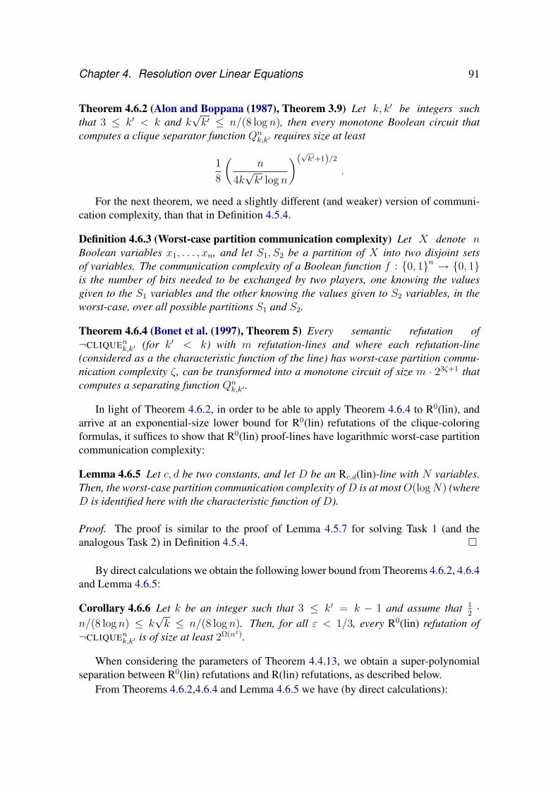
Chapter 4. Resolution over Linear Equations 91
Theorem 4.6.2 (Alon and Boppana (1987), Theorem 3.9) Let k, k′ be integers suchthat 3 ≤ k′ < k and k
√k′ ≤ n/(8 log n), then every monotone Boolean circuit that
computes a clique separator function Qnk,k′ requires size at least
1
8
(n
4k√k′ log n
)(√k′+1)/2
.
For the next theorem, we need a slightly different (and weaker) version of communi-cation complexity, than that in Definition 4.5.4.
Definition 4.6.3 (Worst-case partition communication complexity) Let X denote nBoolean variables x1, . . . , xn, and let S1, S2 be a partition of X into two disjoint setsof variables. The communication complexity of a Boolean function f : 0, 1n → 0, 1is the number of bits needed to be exchanged by two players, one knowing the valuesgiven to the S1 variables and the other knowing the values given to S2 variables, in theworst-case, over all possible partitions S1 and S2.
Theorem 4.6.4 (Bonet et al. (1997), Theorem 5) Every semantic refutation of¬CLIQUEnk,k′ (for k′ < k) with m refutation-lines and where each refutation-line(considered as a the characteristic function of the line) has worst-case partition commu-nication complexity ζ , can be transformed into a monotone circuit of size m · 23ζ+1 thatcomputes a separating function Qn
k,k′ .
In light of Theorem 4.6.2, in order to be able to apply Theorem 4.6.4 to R0(lin), andarrive at an exponential-size lower bound for R0(lin) refutations of the clique-coloringformulas, it suffices to show that R0(lin) proof-lines have logarithmic worst-case partitioncommunication complexity:
Lemma 4.6.5 Let c, d be two constants, and let D be an Rc,d(lin)-line with N variables.Then, the worst-case partition communication complexity ofD is at mostO(logN) (whereD is identified here with the characteristic function of D).
Proof. The proof is similar to the proof of Lemma 4.5.7 for solving Task 1 (and theanalogous Task 2) in Definition 4.5.4.
By direct calculations we obtain the following lower bound from Theorems 4.6.2, 4.6.4and Lemma 4.6.5:
Corollary 4.6.6 Let k be an integer such that 3 ≤ k′ = k − 1 and assume that 12·
n/(8 log n) ≤ k√k ≤ n/(8 log n). Then, for all ε < 1/3, every R0(lin) refutation of
¬CLIQUEnk,k′ is of size at least 2Ω(nε).
When considering the parameters of Theorem 4.4.13, we obtain a super-polynomialseparation between R0(lin) refutations and R(lin) refutations, as described below.
From Theorems 4.6.2,4.6.4 and Lemma 4.6.5 we have (by direct calculations):

Chapter 4. Resolution over Linear Equations 92
Corollary 4.6.7 Let k =√n and k′ = (log n)2/8 log log n. Then, every R0(lin) refutation
of ¬CLIQUEnk,k′ has size at least nΩ(
logn√log logn
).
By Corollary 4.4.14, R(lin) admits polynomial-size in n refutations of ¬CLIQUEnk,k′under the parameters in Corollary 4.6.7. Thus we obtain the following separation result:
Corollary 4.6.8 R(lin) is super-polynomially stronger than R0(lin).
Comment: Note that we do not need to assume that the coefficients in “R0(lin) proof-lines” are constants for the lower bound argument. If the coefficients in “R0(lin) proofs-lines” are only polynomially bounded (in the number of variables) then the same lowerbound as in Corollary 4.6.7 also applies. This is because “R0(lin) proof-lines” in whichcoefficients are polynomially bounded integers, still have low (that is, logarithmic) worst-case partition communication complexity.
4.7 Relations with Extensions of Cutting PlanesIn this section we tie some loose ends by showing that, in full generality, R(lin) polyno-mially simulates R(CP) with polynomially bounded coefficients, denoted R(CP*). Firstwe define the R(CP*) proof system – introduced in Krajıcek (1998) – which is a commonextension of resolution and CP* (the latter is cutting planes with polynomially boundedcoefficients). The system R(CP*), thus, is essentially resolution operating with disjunc-tions of linear inequalities (with polynomially bounded integral coefficients) augmentedwith the cutting planes inference rules.
A linear inequality is written as
~a · ~x ≥ a0 , (4.44)
where ~a is a vector of integral coefficients a1, . . . , an, ~x is a vector of variables x1, . . . , xn,and a0 is an integer. The size of the linear inequality (4.44) is the sum of all a0, . . . , anwritten in unary notation (this is similar to the size of linear equations in R(lin)). Adisjunction of linear inequalities is just a disjunction of inequalities of the form in (4.44).The semantics of a disjunction of inequalities is the natural one, that is, a disjunction istrue under an assignment of integral values to ~x if and only if at least one of the inequalitiesis true under the assignment. The size of a disjunction of linear inequalities is the totalsize of all linear inequalities in it. We can also add in the obvious way linear inequalities,that is, if L1 is the linear inequality ~a · ~x ≥ a0 and L2 is the linear inequality ~b · ~x ≥ b0,then L1 + L2 is the linear inequality (~a+~b) · ~x ≥ a0 + b0.
The proof system R(CP*) operates with disjunctions of linear inequalities with inte-gral coefficients (written in unary notation), and is defined as follows (our formulation issimilar to that in Kojevnikov (2007)):12
12When we allow coefficients to be written in binary notation, instead of unary notation, the resultingproof system is denoted R(CP).

Chapter 4. Resolution over Linear Equations 93
Definition 4.7.1 (R(CP*)) Let K := K1, . . . , Km be a collection of disjunctions oflinear inequalities (whose coefficients are written in unary notation). An R(CP*)-prooffrom K of a disjunction of linear inequalities D is a finite sequence π = (D1, ..., D`) ofdisjunctions of linear inequalities, such thatD` = D and for each i ∈ [`]: either Di = Kj
for some j ∈ [m]; or Di is one of the following R(CP*)-axioms:
1. xi ≥ 0, for any variable xi;
2. −xi ≥ −1, for any variable xi;
3. (~a · ~x ≥ a0) ∨ (−~a · ~x ≥ 1− a0), where all coefficients (including a0) are integers;
or Di was deduced from previous lines by one of the following R(CP*)-inference rules:
1. Let A,B be two, possibly empty, disjunctions of linear inequalities and let L1, L2
be two linear inequalities.
From A ∨ L1 and B ∨ L2 derive A ∨B ∨ (L1 + L2).
2. Let L be some linear equation.
From a, possibly empty, disjunction of linear equations A derive A ∨ L.
3. Let A be a, possibly empty, disjunction of linear equations.
From A ∨ (0 ≥ 1) derive A.
4. Let c be a non-negative integer.
From (~a · ~x ≥ a0) ∨ A derive (c~a · ~x ≥ ca0) ∨ A.
5. Let A be a, possibly empty, disjunction of linear inequalities, and let c ≥ 1 be aninteger.
From (c~a · ~x ≥ a0) ∨ A derive (a · ~x ≥ da0/ce) ∨ A.
An R(CP*) refutation of a collection of disjunctions of linear inequalities K is a proof ofthe empty disjunction from K. The size of a proof π in R(CP*) is the total size of all thedisjunctions of linear inequalities in π, denoted |π|.
In order for R(lin) to simulate R(CP*) proofs, we need to fix the following translationscheme. Every linear inequality L of the form ~a · ~x ≥ a0 is translated into the followingdisjunction, denoted L:
(~a · ~x = a0) ∨ (~a · ~x = a0 + 1) ∨ · · · ∨ (~a · ~x = a0 + k) , (4.45)
where k is such that a0 +k equals the sum of all positive coefficients in ~a, that is, a0 +k =max~x∈0,1n (~a · ~x) (in case the sum of all positive coefficients in ~a is less than a0, then weput k = 0). An inequality with no variables of the form 0 ≥ a0 is translated into 0 = a0
in case it is false (that is, in case 0 < a0), and into 0 = 0 in case it is true (that is, in case0 ≥ a0). Note that since the coefficients of linear inequalities (and linear equations) are

Chapter 4. Resolution over Linear Equations 94
written in unary notation, any linear inequality of size s translates into a disjunction oflinear equations of size O(s2). Clearly, every 0, 1 assignment to the variables ~x satisfiesL if and only if it satisfies its translation L. A disjunction of linear inequalities D istranslated into the disjunction of the translations of all the linear inequalities in it, denotedD. A collection K := K1, . . . , Km of disjunctions of linear inequalities, is translatedinto the collection
K1, . . . , Km
.
Theorem 4.7.2 R(lin) polynomially-simulates R(CP*). In other words, if π is an R(CP*)proof of a linear inequality D from a collection of disjunctions of linear inequalitiesK1, . . . , Kt, then there is an R(lin) proof of D from K1, . . . , Kt whose size is polynomialin |π|.
Proof. By induction on the number of proof-lines in π.Base case: Here we only need to show that the axioms of R(CP*) translates into
axioms of R(lin), or can be derived with polynomial-size (in the size of the original R(CP*)axiom) R(lin) derivations (from R(lin)’s axioms).
R(CP*) axiom number (1): xi ≥ 0 translates into the R(lin) axiom (xi = 0)∨(xi = 1).R(CP*) axiom number (2): −xi ≥ −1, translates into (−xi = −1)∨ (−xi = 0). From
the Boolean axiom (xi = 1) ∨ (xi = 0) of R(lin), one can derive with a constant-sizeR(lin) proof the line (−xi = −1) ∨ (−xi = 0) (for instance, by subtracting twice eachequation in (xi = 1) ∨ (xi = 0) from itself).
R(CP*) axiom number (3): (~a ·~x ≥ a0)∨(−~a ·~x ≥ 1−a0). The inequality (~a ·~x ≥ a0)translates into
h∨b=a0
(~a · ~x = b) ,
where h is the maximal value of ~a · ~x over 0, 1 assignments to ~x (that is, h is just the sumof all positive coefficients in ~a). The inequality (−~a · ~x ≥ 1− a0) translates into
f∨b=1−a0
(−~a · ~x = b) ,
where f is the maximal value of−~a ·~x over 0, 1 assignments to ~x (that is, f is just the sumof all negative coefficients in ~a). Note that one can always flip the sign of any equation~a · ~x = b in R(lin). This is done, for instance, by subtracting twice ~a · ~x = b from itself.So overall R(CP*) axiom number (3) translates into
h∨b=a0
(~a · ~x = b) ∨f∨
b=1−a0
(−~a · ~x = b) ,
that can be converted inside R(lin) into
a0−1∨b=−f
(~a · ~x = b) ∨h∨
b=a0
(~a · ~x = b) . (4.46)

Chapter 4. Resolution over Linear Equations 95
LetA′ := −f,−f + 1, . . . , a0 − 1, a0, a0 + 1, . . . , h and letA be the set of all possiblevalues that ~a · ~x can get over all possible Boolean assignments to ~x. Notice that A ⊆ A′.By Lemma 4.2.5, for any ~a · ~x, there is a polynomial-size (in the size of the linear form~a · ~x) derivation of
∨α∈A(~a · ~x = α). By using the R(lin) weakening rule we can then
derive∨α∈A′(~a · ~x = α) which is equal to (4.46).
Induction step: Here we simply need to show how to polynomially simulate insideR(lin) every inference rule application of R(CP*).
Rule (1): Let A,B be two disjunctions of linear inequalities and let L1, L2 be two linearinequalities. Assume we already have a R(lin) proofs of A ∨ L1 and B ∨ L2. We need toderive A∨ B ∨ L1 + L2. Corollary 4.2.4 shows that there is a polynomial-size (in the sizeof L1 and L2; which is polynomial in the size of L1 and L2) derivation of L1 + L2 fromL1 and L2, from which the desired derivation immediately follows.
Rule (2): The simulation of this rule in R(lin) is done using the R(lin) weakening rule.
Rule (3): The simulation of this rule in R(lin) is done using the R(lin) simplification rule(remember that 0 ≥ 1 translates into 0 = 1 under our translation scheme).
Rule (4): Let c be a non-negative integer. We need to derive (c~a · ~x ≥ ca0) ∨ A from(~a · ~x ≥ a0)∨ A in R(lin). This amounts only to “adding together” c times the disjunction(~a · ~x ≥ a0) in (~a · ~x ≥ a0)∨ A. This can be achieved by c many applications of Corollary
4.2.4. We omit the details.
Rule (5): We need to derive (~a · ~x ≥ da0/ce)∨ A, from (c~a · ~x ≥ a0)∨ A. Consider thedisjunction of linear equations (c~a · ~x ≥ a0), which can be written as:
(c~a · ~x = a0) ∨ (c~a · ~x = a0 + 1) ∨ . . . ∨ (c~a · ~x = a0 + r) , (4.47)
where a0 + r is the maximal value c~a · ~x can get over 0, 1 assignments to ~x. By Lemma4.2.5 there is a polynomial-size (in the size of ~a · ~x) R(lin) proof of∨
α∈A
(~a · ~x = α) , (4.48)
where A is the set of all possible values of ~a · ~x over 0, 1 assignments to ~x.We now use (4.47) to cut-off from (4.48) all equations (~a · ~x = β) for all β < da0/ce
(this will give us the desired disjunction of linear equations). Consider the equation (~a·~x =β) in (4.48) for some fixed β < da0/ce. Use the resolution rule of R(lin) to add thisequation to itself c times inside (4.48). We thus obtain
(c~a · ~x = cβ) ∨∨
α∈A\β
(~a · ~x = α) . (4.49)

Chapter 4. Resolution over Linear Equations 96
Since β is an integer and β < da0/ce, we have cβ < a0. Thus, the equation (c~a · ~x = cβ)does not appear in (4.47). We can then successively resolve (c~a · ~x = cβ) in (4.49)with each equation (c~a · ~x = a0), . . . , (c~a · ~x = a0 + r) in (4.47). Hence, we arrive at∨α∈A\β (~a · ~x = α). Overall, we can cut-off all equations (~a · ~x = β), for β < da0/ce,
from (4.48). We then get the disjunction∨α∈A′
(~a · ~x = α) ,
where A′ is the set of all elements of A greater or equal to da0/ce (in other words, allvalues greater or equal to da0/ce that ~a · ~x can get over 0, 1 assignments to ~x). Usingthe weakening rule of R(lin) (if necessary) we can arrive finally at the desired disjunction
(~a · ~x ≥ da0/ce), which concludes the R(lin) simulation of R(CP*)’s inference Rule (5).
4.8 Chapter SummaryIn this chapter we explored extensions of resolution of varying strength that operate withdisjunctions of linear equations instead of clauses. We demonstrated efficient proofs forcounting arguments in resolution over linear equations and its fragments. We showedthat already a proper fragment of resolution over linear equations is capable of efficientlyproving certain hard formulas. We also obtained exponential lower bounds on fragmentsof resolution over linear equations using the monotone interpolation technique, and pro-vided a simulation of full cutting planes proofs with polynomially bounded coefficientsby resolution over linear equations.
In the next chapter we shall link resolution over linear equations with multilinearproofs. Specifically, we show that depth-3 multilinear proofs can polynomially simulateR0(lin) proofs.
Chapter 5
From Resolution over Linear Equationsto Multilinear Proofs
97

Chapter 5. From Resolution over Linear Equations to Multilinear Proofs 98
In this chapter we apply the results about resolution over linear equations from Chapter4 to obtain new results for multilinear proof systems. In particular, we shall demonstratea polynomial simulation of R0(lin) by multilinear proofs operating with depth-3 formu-las. This simulation will rely heavily on the fact that multilinear symmetric polynomialshave small depth-3 multilinear formulas over fields of characteristic 0 (see Preliminaries,Section 2.5.4).
5.1 From R(lin) Proofs to PCR ProofsHere we demonstrate a general and straightforward translation from R(lin) proofs intoPCR proofs over fields of characteristic 0. We use the term “translation” in order to dis-tinguish it from a simulation; since here we are not interested in the size of PCR proofs.In fact we have not defined the size of PCR proofs at all. We shall be interested only inthe number of steps in PCR proofs.
From now on, all polynomials and arithmetic formulas are considered over some fixedfield F of characteristic 0. Recall that any field of characteristic 0 contains (an isomorphiccopy of) the integer numbers, and so we can use integer coefficients in the field.
Definition 5.1.1 (Polynomial translation of R(lin) proof-lines) Let D be a disjunctionof linear equations:(
a(1)1 x1 + . . .+ a(1)
n xn = a(1)0
)∨ · · · ∨
(a
(t)1 x1 + . . .+ a(t)
n xn = a(t)0
). (5.1)
We denote by D its translation into the following polynomial:1(a
(1)1 x1 + . . .+ a(1)
n xn − a(1)0
)· · ·(a
(t)1 x1 + . . .+ a(t)
n xn − a(t)0
). (5.2)
If D is the empty disjunction, we define D to be the polynomial 1.
It is clear that every 0, 1 assignment to the variables in D, satisfies D, if and only if Devaluates to 0 under the assignment.
Proposition 5.1.2 Let π = (D1, . . . , D`) be an R(lin) proof sequence of D`, from somecollection of initial disjunctions of linear equations Q1, . . . , Qm. Then, there exists a PCRproof of D` from Q1, . . . , Qm with at most a polynomial in |π| number of steps.
Proof. We proceed by induction on the number of lines in π. The base case is the trans-lation of the axioms of R(lin) via the translation scheme in Definition 5.1.1. An R(lin)Boolean axiom (xi = 0) ∨ (xi = 1) is translated into xi · (xi − 1) which is already aBoolean axiom of PCR.
1This notation should not be confused with the same notation in Section 4.4.3.

Chapter 5. From Resolution over Linear Equations to Multilinear Proofs 99
For the induction step, we translate an R(lin) inference rule application into apolynomial-size PCR proof sequence as follows. We use the following simple claim:
Claim: Let p and q be two polynomials and let s be the minimal size of an arithmeticformula computing q. Then one can derive from p in PCR the product q · p, with only apolynomial in s number of steps.
Proof of claim: By induction on s. Claim
Assume that Di = Dj ∨L was derived from Dj using the weakening inference rule ofR(lin), where j < i ≤ ` and L is some linear equation. Then, by Claim 5.1, Di = Dj · Lcan be derived from Dj with a derivation of at most polynomial in |Dj ∨ L| many steps.
Assume thatDi was derived fromDj whereDj isDi∨(0 = k), using the simplificationinference rule of R(lin), where j < i ≤ ` and k is a non-zero integer. Then, Di can bederived from Dj = Di · −k by multiplying with −k−1 (via the Addition rule of PCR).
Thus, it remains to simulate the resolution rule application of R(lin). Let A,B be twodisjunctions of linear equations and assume that A ∨ B ∨ ((~a − ~b) · ~x = a0 − b0) wasderived in π from A ∨ (~a · ~x = a0) and B ∨ (~b · ~x = b0).
We need to derive A · B · ((~a−~b) ·~x−a0 + b0) from A · (~a ·~x−a0) and B · (~b ·~x− b0).This is done by multiplying A · (~a · ~x − a0) with B and multiplying B · (~b · ~x − b0) withA (using Claim 5.1), and then subtracting the resulted polynomials from each other.
Remark: When translating R(lin) proofs into PCR proofs we actually do not make anyuse of the “negative” variables x1, . . . , xn. Nevertheless, the multilinear proof systemsmake use of these variables in order to polynomially simulate PCR proofs (see Theorem3.3.1 and its proof in Chapter 3 Section 3.3).
We shall need the following corollary in the sequel:
Corollary 5.1.3 Let c, d be two constants, let π = D1, . . . , D` be an R(lin) proof of D`
using only Rc,d(lin)-lines, and let s be the maximal size of an Rc,d(lin)-line in π. Then thereare two constants c′, d′ that depend only on c, d and a PCR proof π′ of D` with polynomial-size in |π| number of steps, and such that every line of π′ has size at most polynomial in sand is a translation (via Definition 5.1.1) of an Rc′,d′(lin)-line.
Proof. The simulation of R(lin) by PCR shown above, can be thought of as, first, consid-ering D1, . . . , D` as the “skeleton” of a PCR proof of D`. And second, for each Di thatwas deduced by one of R(lin)’s inference rules from previous lines, one inserts the cor-responding PCR proof sequence that simulates the appropriate inference rule application(as described in the proof of Proposition 5.1.2). By definition, those PCR proof-lines thatcorrespond to lines in the skeleton D1, . . . , D` are translations of Rc,d(lin)-lines (with sizeat most polynomial in s). Thus, to conclude the proof of the corollary, one needs onlyto check that for any Rc,d(lin)-line Di that was deduced by one of R(lin)’s inference rulesfrom previous Rc,d(lin)-lines (as demonstrated in the proof of Proposition 5.1.2), the in-serted corresponding PCR proof sequence uses only translations of Rc′,d′(lin)-lines (with
Chapter 5. From Resolution over Linear Equations to Multilinear Proofs 100
size polynomial in s), for two constants c′, d′ that depend only on c, d. This can be verifiedby a straightforward inspection.
5.2 From PCR Proofs to Multilinear ProofsFirst recall the general simulation result (Theorem 3.3.1) proved in Chapter 3. This theo-rem states the following: Let π be a PCR refutation of some initial collection of multilinearpolynomials Q over some fixed field. Assume that π has polynomially many steps (thatis, the number of proof lines in the PCR proof sequence is polynomial). If the multilin-earization (namely, the result of applying the M[·] operator [Definition 2.5.2]) of each ofthe polynomials in π has a polynomial-size depth d multilinear formula (with a plus gateat the root), then there is a polynomial-size depth-d fMC refutation of Q.
5.2.1 Multilinearization of Polynomials
Here we show that multilinear proofs operating with depth-3 multilinear formulas (that is,depth-3 fMC) over fields of characteristic 0 polynomially simulate R0(lin) proofs. In lightof Proposition 5.1.3 and Theorem 3.3.1, to this end it suffices to show that for constantsc, d, any Rc,d(lin)-line D translates into a corresponding polynomial p (via the translationin Definition 5.1.1) such that M[p] has a multilinear formula of size polynomial (in thenumber of variables) and depth at most 3 (with a plus gate at the root) over fields ofcharacteristic 0.
We need the following simple properties (given without a proof):
Proposition 5.2.1 Fix a field F and let X be a finite set of variables.
• If p, q are two symmetric polynomials over X , then the product p · q is also asymmetric polynomial over X;
• If p is a symmetric polynomial over X , then M[p] is a multilinear symmetric poly-nomial over X .
From Theorem 2.5.4 and Proposition 5.2.1 we get:
Corollary 5.2.2 Let F be a field of characteristic 0 and let X be a set of ` variables. If pis a product of (one or more) symmetric polynomials overX (over the field F), then M[p]has a depth-3 multilinear formula of size polynomial (in `), with a plus gate at the root.
We shall also need the following more general proposition, which might be interestingby itself:
Proposition 5.2.3 Let F be a field of characteristic 0. For a constant c, let X1, . . . , Xc bec finite sets of variables (not necessarily disjoint), where Σc
i=1|Xi| = ` . Let f1, . . . , fc bec symmetric polynomials over X1, . . . , Xc (over the field F), respectively. Then, there isa depth-3 multilinear formula for M[f1 · · · fc] of size polynomial (in `), with a plus gateat the root.

Chapter 5. From Resolution over Linear Equations to Multilinear Proofs 101
Remark. Note the difference between Corollary 5.2.2 and Proposition 5.2.3. Corollary5.2.2 speaks about a (finite) unbounded product of symmetric polynomials over the sameset of variables. On the other hand, Proposition 5.2.3 speaks about a product of con-stant number of symmetric polynomials over different (but not necessarily disjoint) setsof variables.
Proof. We shall need the following two basic claims (given without a proof).
Claim: Let X be a set of ` variables x1, . . . , x`, and let p1, p2 be two multilinearpolynomials over X such that for all 0, 1 assignments to x1, . . . , x`, p1(x1, . . . , x`) =p2(x1, . . . , x`). Then p1 = p2 as formal polynomials.
Since symmetric polynomials are invariant under renaming of variables then restrictedto 0, 1 assignments the values of symmetric polynomials are determined only by the num-ber of 1’s in their input variables. Formally, if p is a symmetric polynomial of degree dfrom F[X] in ` variables, then there is a polynomial h of degree at most d in one variable,such that for 0, 1 assignments to x1, . . . , x`, p(x1, . . . , x`) = h(x1+. . .+x`). Hence, if welet Y1, . . . , Ym be pairwise disjoint subsets of X = x1, . . . , x`, such that
⊎mi=1 Yi = X ,
then we have the following:
Claim: Let p be a symmetric polynomial from F[X] of degree d, then there is a polynomialh of degree at most d in m variables, such that for all 0, 1 assignments to x1, . . . , x`,
p(x1, . . . , x`) = h
(∑xi∈Y1
xi, . . . ,∑xi∈Ym
xi
).
We are now ready to prove Proposition 5.2.3. Let X :=⋃ci=1Xi. Let m := 2c and
partition X into at most m disjoint subsets as follows. For every J ⊆ [c], let XJ :=⋂i∈J Xi \
⋃i∈[c]\J Xi and define the abbreviation
zJ :=∑xi∈XJ
xi . (5.3)
(This way, the variables in Xi are exactly the variables that occur in all zJ , such thati ∈ J ⊆ [c].) Let J1, . . . , Jm be all the subsets of [c], and let zk denote zJk , for every1 ≤ k ≤ m.
We clearly have,
M
[c∏i=1
fi
]= M
[c∏i=1
M[fi]
]. (5.4)
By Proposition 5.2.1, for all 1 ≤ i ≤ c, M[fi] is a (multilinear) symmetric polynomial.Thus, by Claim 5.2.1, for all 1 ≤ i ≤ c there exists a polynomial gi(y1, . . . , ym) of degreeat most ` (with at most m variables), such that M[fi] = gi(z1, . . . , zm) for all assignments
Chapter 5. From Resolution over Linear Equations to Multilinear Proofs 102
of 0, 1 values to the variables inXi (note that gi(y1, . . . , ym) is not necessarily a multilinearpolynomial in the yj’s).2
Hence, by (5.4) for all assignments of 0, 1 to the variables in X,
M
[c∏i=1
fi
]= M
[c∏i=1
gi(z1, . . . , zm)
](5.5)
(note that the multilinearization operator M[·] in the right hand side of (5.5) operates onthe polynomial
∏ci gi(z1, . . . , zm) considered as a polynomial in the X variables).
Therefore, by Claim 5.2.1, the two sides of (5.5) are equal as formal polynomials (overX). Since c and m are constants,
∏ci gi(y1, . . . , ym) can be written as a sum of polynomi-
ally many monomials in the variables y1, . . . , ym. Thus, when substituting zj’s for yj’s (forall 1 ≤ j ≤ m),
∏ci gi(z1, . . . , zm) can be written as a sum of polynomially many prod-
ucts of the form∏m
j=1 zejj (where the ej’s stand for some non-negative integers). Hence,
by linearity of M[·], the right hand side of (5.5) can be written as a sum of polynomiallymany terms of the form M
[∏mj=1 z
ejj
]. It remains only to prove the following:
Claim: Every polynomial of the form M[∏m
j=1 zejj
](where the ej’s stand for some non-
negative integers) has a depth 3 multilinear formula (in the variables in X) of size polyno-mial in ` and a plus gate at the root .
Proof of claim: Since the sets of variables that occur in each of the zj’s are pairwise
disjoint, M[∏m
j=1 zejj
]=∏m
j=1 M[zejj
]. For every 1 ≤ j ≤ m, zejj is a product of
symmetric polynomials (in (not necessarily all) the variables in X). Thus, by Corollary5.2.2, M
[zejj
]can be written as a sum of polynomially (in `) many products of linear
polynomials (in other words, a polynomial-size leveled depth 3 multilinear formula witha plus gate at the root). Since m is a constant,
∏mj=1 M
[zejj
]can be written as a sum
of polynomially many terms, where each term is a product of (polynomially many) linearpolynomials over disjoint sets of variables. In other words, we have reached a polynomial-size (in `) depth 3 multilinear formula. Claim
This completes the proof of Proposition 5.2.3.
Lemma 5.2.4 Let s, t be two constants that do not depend on n, let D be an Rs,t(lin)-line with n variables and let p = D (see Definition 5.1.1). Then, M[p] has a depth-3multilinear formula over fields of characteristic 0, with a plus gate at the root and size atmost polynomial in the size of D.
Proof. Assume that the underlying variables of D are ~x = x1 . . . , xn. By assumption, wecan partition the disjunction D into a constant number t of disjuncts, where one disjunct
2For any 1 ≤ k ≤ m, the variable yk actually occurs in gi if and only if i ∈ Jk. The other variables ykare still indicated for ease of writing.

Chapter 5. From Resolution over Linear Equations to Multilinear Proofs 103
is a (possibly empty, translation of a) clause C, and all other disjuncts have the followingform:
m∨i=1
(~a · ~x = `i) , (5.6)
where the `i’s are integers, m is not necessarily bounded and ~a denotes a vector of nconstant integer coefficients, each having absolute value at most s.
Suppose that the clause C is∨i∈I xi ∨
∨j∈J ¬xj , and let us denote by q =
∏i∈I(xi−
1) ·∏j∈J xj the polynomial representing C.Consider a disjunct as shown in (5.6). Since the coefficients ~a are constants (having
absolute value at most s), ~a ·~x can be written as a sum of constant number of linear forms,each with the same constant coefficient. In other words, ~a·~x can be written as z1 +. . .+zd,for some constant d, where for all i ∈ [d]:
zi := b ·∑j∈J
xj , (5.7)
for some J ⊆ [n] and some constant integer b. We shall assume without loss of generalitythat d is the same constant for every disjunct of the form (5.6) inside D (otherwise, take dto be the maximal such d).
Thus, (5.6) is translated (via the translation scheme in Definition 5.1.1) into:m∏i=1
(z1 + ...+ zd − `i) . (5.8)
By fully expanding the product in (5.8), we arrive at:
∑r1+...+rd+1=m
(αrd+1
·d∏
k=1
zrkk
), (5.9)
where the ri’s are non-negative integers, and where the αr’s, for every 0 ≤ r ≤ m are justinteger coefficients, formally defined as follows (this definition is not essential; we presentit only for the sake of concreteness):
αr :=∑U⊆[m]|U |=r
∏j∈U
(−`j) . (5.10)
Claim: The polynomial D (the polynomial translation of D) is a linear combination (overF) of polynomially (in |D|) many terms, such that each term can be written as
q ·∏k∈K
zrkk ,
where K is a collection of a constant number of indices, rk’s are non-negative integers,and the zk’s and q are as above (that is, the zk’s are linear forms, where each zk has a singlecoefficient for all variables in it, as in (5.7), and q is a polynomial translation of a clause).

Chapter 5. From Resolution over Linear Equations to Multilinear Proofs 104
Proof of claim: By assumption, the total number of disjuncts of the form (5.6) in D is≤ t.Consider the polynomial (5.9) above. In D, we actually need to multiply at most t manypolynomials of the form shown in (5.9) and the polynomial q.
For every j ∈ [t] we write the (single) linear form in the jth disjunct as a sum ofconstantly many linear forms zj,1 + . . . + zj,d, where each linear form zj,k has the samecoefficient for every variable in it. Thus, D can be written as:
q ·t∏
j=1
∑
r1+...+rd+1=mj
(α(j)rd+1·
d∏k=1
zrkj,k
)︸ ︷︷ ︸
(?)
, (5.11)
(where the mj’s are not bounded, and the coefficients α(j)rd+1 are as defined in (5.10) except
that here we add the index (j) to denote that they depend on the jth disjunct inD). Denotethe maximal mj , for all j ∈ [t], by m0. The size of D, denoted |D|, is at least m0. Notethat since d is a constant, the number of summands in each (middle) sum in (5.11) ispolynomial in m0, which is at most polynomial in |D|. Thus, by expanding the outermostproduct in (5.11), we arrive at a sum of polynomially in |D| many summands. Eachsummand in this sum is a product of t terms of the form designated by (?) in Equation(5.11), multiplied by q. Claim
It remains to apply the multilinearization operator (Definition 2.5.2) on D, and verifythat the resulting polynomial has a depth-3 multilinear formula with a plus gate at the rootand of polynomial-size (in |D|). Since M[·] is a linear operator, it suffices to show thatwhen applying M[·] on each summand in D, as described in Claim 5.2.1, one obtains a(multilinear) polynomial that has a depth-3 multilinear formula with a plus gate at the root,and of polynomial-size in the number of variables n (note that clearly n ≤ |D|). This isestablished in the following claim:
Claim: The polynomial M[q ·∏k∈K z
rkk
]has a depth-3 multilinear formula of
polynomial-size in n (the overall number of variables) and with a plus gate at the root(over fields of characteristic 0), under the same notation as in Claim 5.2.1.
Proof of claim: Recall that a power of a symmetric polynomial is a symmetric polynomialin itself. Since each zk (for all k ∈ K) is a symmetric polynomial, then its power zrkk isalso symmetric. The polynomial q is a translation of a clause, hence it is a product of twosymmetric polynomials: the symmetric polynomial that is the translation of the disjunctionof literals with positive signs, and the symmetric polynomial that is the translation of thedisjunction of literals with negative signs. Therefore, q ·∏k∈K z
rkk is a product of constant
number of symmetric polynomials. By Proposition 5.2.3 M[q ·∏k∈K z
rkk
](where here
the M[·] operator operates on the ~x variables in the zk’s and q) is a polynomial for whichthere is a polynomial-size (in n) depth-3 multilinear formula with a plus gate at the root(over fields of characteristic 0). Claim

Chapter 5. From Resolution over Linear Equations to Multilinear Proofs 105
We now come to the main result of this chapter.
Corollary 5.2.5 Multilinear proofs operating with depth-3 multilinear formulas (that is,depth-3 fMC proofs) polynomially-simulate R0(lin) proofs.
Proof. Immediate from Corollary 5.1.3, Theorem 3.3.1 and Proposition 5.2.4.For the sake of clarity we repeat the chain of transformations needed to prove the sim-
ulation. Let π be a given R0(lin) proof that uses only Rc,d(lin)-lines, for c, d two constantintegers. We first use Corollary 5.1.3 to transform π into a PCR proof π′, with number ofsteps that is at most polynomial in |π|, and where each line in π′ is a polynomial transla-tion of some Rc,d(lin)-line with size at most polynomial in the maximal line in π (which isclearly at most polynomial in |π|). Thus, by Proposition 5.2.4 each polynomial in π′ hasa corresponding multilinear polynomial with a polynomial-size in |π| depth-3 multilinearformula (and a plus gate at the root). Therefore, by Theorem 3.3.1, we can transform π′
into a depth-3 fMC proof with only a polynomial (in |π|) increase in size.
5.3 Applications to Multilinear Proofs: Small Depth-3Multilinear Proofs
5.3.0.1 The Pigeonhole Principle
Recall the propositional formulation of the pigeonhole principle described in Chapter 4Section 4.4.1. The two sets of clauses in (4.24) translate via Definition 3.0.7 to the follow-ing set of polynomials:
Pigeons : ∀i ∈ [m], xi,1 · · · xi,nHoles : ∀i < j ∈ [m]∀k ∈ [n], xi,k · xj,k (5.12)
By Theorem 4.4.4, R0(lin) admits polynomial-size (in n) refutations of the m to npigeonhole principle (for any m > n) (as defined in Definition 4.4.1). Thus, Corollary5.2.5 yields:
Theorem 5.3.1 For any m > n there are polynomial-size (in n) depth-3 fMC refutationsof the m to n pigeonhole principle PHPmn (over fields of characteristic 0).
Haken (1985) showed an exponential lower bound on the size of resolution refutationsof the pigeonhole principle (where the number of holes is n and the number of pigeons isn+ 1). Pitassi et al. (1993) and, independently, Krajıcek et al. (1995) showed exponentiallower bounds on the size of proofs of the pigeonhole principle in bounded-depth Frege(again, where the number of holes is n and number of pigeons is n+ 1). Razborov (1998)and, subsequently, Impagliazzo et al. (1999) showed exponential lower bounds on the
Chapter 5. From Resolution over Linear Equations to Multilinear Proofs 106
size (and degree) of PC-refutations of a different low degree version of the pigeonholeprinciple. In this low degree version the Pigeon polynomials of (5.12) are replaced by1 − (xi,1 + . . . + xi,n), for all i ∈ [m]. This low degree version is not a translation ofa CNF formula. Our upper bound is also applicable to this low-degree version of thepigeonhole principle (however, this would not yield a separation of fMC from PC andPCR as we consider these proof systems as proof systems for (polynomial translations of)CNF formulas).
Grigoriev and Hirsch (2003) showed polynomial size refutations of the pigeonholeprinciple (i.e., polynomials (5.12)) for a formal (syntactic) propositional proof systemdenotedF-PC (see the discussion on the fMC proof system in Chapter 3 and Chapter 6 formore on syntactic algebraic proof systems) that manipulates general arithmetic formulas.Their refutations operate with general arithmetic formulas of constant-depth.
By the discussion above we have:
Corollary 5.3.2 Depth-3 fMC over fields of characteristic 0 has an exponential gap overresolution and bounded-depth Frege for the pigeonhole principle.
Since depth-3 fMC polynomially simulates resolution (Proposition 3.2.2) then byCorollary 5.3.2 depth-3 fMC is strictly stronger than resolution.
5.3.0.2 Tseitin mod p Formulas
Corollary 5.2.5 and Theorem 4.4.9 yield:
Theorem 5.3.3 LetG be an r-regular graph with n vertices, where r is a constant, and fixsome modulus p. Then there are polynomial-size (in n) depth-3 fMC refutations of Tseitinmod p formulas BTSG,p (over fields of characteristic 0).
The polynomial-size refutations of Tseitin graph tautologies here are different thanthose demonstrated in Chapter 3 (Section 3.5). Theorem 5.3.3 establishes polynomial-size refutations over any field of characteristic 0 of Tseitin mod p formulas, whereas theformer proofs required the field to contain a primitive pth root of unity. On the otherhand, the refutations in Section 3.5 of Tseitin mod p formulas do not make any use of thesemantic nature of the fMC proof system, in the sense that they do not utilize the fact thatthe base field is of characteristic 0. (The latter fact enables one to efficiently represent anysymmetric [multilinear] polynomial by a depth-3 multilinear formula.)
5.4 Chapter SummaryIn this chapter we linked together the results of the previous two chapters (Chapters 3, 4).Specifically, we showed that depth-3 multilinear proofs can already polynomial simulatea certain considerably strong fragment of R(lin) (namely, R0(lin)). As a consequencewe obtained polynomial upper bounds on depth-3 multilinear proofs of the propositional

Chapter 5. From Resolution over Linear Equations to Multilinear Proofs 107
pigeonhole principle and the Tseitin’s mod p formulas (the latter is different from the shortproofs demonstrated in Chapter 3).

Chapter 6
Symbolic Proofs of PolynomialIdentities: From Semantic to SyntacticAlgebraic Proofs
109

Chapter 6. Symbolic Proofs of Polynomial Identities 110
This chapter aims at developing further the theory of algebraic proof complexity. Here,instead of establishing propositional tautologies, we shall consider algebraic proof systemsestablishing that a given arithmetic formula computes the zero polynomial (or, equiva-lently, that two given arithmetic formulas compute the same polynomial). We begin withthe basic definition of the model and then we continue (in Section 6.5) with the problemof proving lower bounds.
6.1 PreliminariesFor a graph G we write |G| to denote the number of vertices in G. For an edge directedfrom u to v in G, we also say that u points to v.
Assumptions on arithmetic formulas in this chapter. In this chapter it will be con-venient to consider all arithmetic formulas as labeled trees with fan-in at most two andwhere field elements can only label leaves, and not edges (compare this to the definitionof arithmetic formulas in Section 2.5.1). An arithmetic with a plus or product gate at theroot is said to be a plus formula or product formula, respectively. Given an arithmeticformula Φ a subformula of Φ is any (not necessarily proper) subtree of Φ. We say that anarithmetic formula ϕ occurs in an arithmetic formula ϕ′ if ϕ is a subformula of ϕ′. In thiscase we also say that ϕ′ contains ϕ as a subformula.
We write Φ1 ≡ Φ2 if Φ1 and Φ2 are two syntactically equal formulas (equal as labeledtrees; not to be confused with equality between polynomials). For a formula Φ and a nodev in Φ, we write Φv to denote the subformula of Φ whose root is v. We write Φψv todenote the formula Φ where the subtree rooted by v in Φ is replaced1 by ψ. We writeΦψ (without explicitly displaying v) to mean that ψ is a subformula of Φ.
Constant-depth arithmetic formulas. We shall consider bounded-depth formulas.Since we deal in this chapter with formulas with fan-in two, a depth-d formula will meanthat there is an a priori constant d that bounds the number of alternations between plus andproduct gates in every path in the formula-graph (given a path p from the root to a leaf,the number of alternations between plus and product gates is the number of alternationsbetween consecutive blocks of the same gate-labels). A formula Φ is said to be a ΣΠΣ . . .formula (where ΣΠΣ . . . has d ≥ 1 symbols) if every path in Φ starting at the root andending in the immediate ancestor of a leaf in the formula-graph of Φ is labeled with a blockof (zero or more) consecutive plus gates followed by a block of (zero or more) consecu-tive product gates and so forth (d times). If moreover, a ΣΠΣ . . . (with d ≥ 1 symbols)formula Φ contains a path starting at the root and ending in the immediate ancestor of aleaf that is labeled with a block of one or more consecutive plus gates followed by a blockof one or more consecutive product gates and so forth (d times), then we say that Φ is aproper ΣΠΣ . . . formula. The definition of (proper) ΠΣΠ . . . formulas is similar.
1Note that Φv is identified here with the labeled tree rooted in v, and not with all the formulas that areequivalent to the labeled tree rooted in v. In other words, when we replace Φv by ψ in Φ, we only replacethe subtree of Φ whose root is v, by the tree ψ.

Chapter 6. Symbolic Proofs of Polynomial Identities 111
Comment: When considering depth-3 formulas we shall slightly change the definitionof depth (see Section 6.2.1) in order to conform to the standard definition of depth-3arithmetic formulas (that is, as a sum of products of linear forms).
Notational conventions. In this chapter we deal exclusively with arithmetic formulas,and so we will often use the term “formula” to mean an arithmetic formula. Recall thatgiven two formulas Φ1 and Φ2, we write Φ1 + Φ2 and Φ1 × Φ2 to designate the formulaswith a plus (respectively, product) gate at the root and Φ1,Φ2 as its two children. Wewill also use parenthesis to designate explicitly the structure of formulas. For example,(x1 + x2) + (x3 + x4) means that (x1 + x2) and (x3 + x4) are the two subformulasattached to the root gate (while, (x2 + x3), for instance, is not a subformula of the mainformula). Most often we will not care for the associativity and order of multiplication andaddition, to the effect that we shall not write explicitly the parentheses in formulas, likein Φ1 × Φ2 × Φ3. Further, we write
∏i∈I Φi, where I is some set of indices, to mean the
product formula whose products are all Φi (for i ∈ I), where we ignore the associativity ofsubformulas (formally, every product gate in this formula is still of fun-in 2; though this isnot essential). Similarly, we will write
∑i∈I Φi for the plus formula of all Φi (i ∈ I). Also,
we will sometimes abuse notation by identifying arithmetic formulas with the polynomialsthey compute.
6.2 Analytic Symbolic Proofs of Polynomial IdentitiesLet us fix our underlying field F. Unless otherwise stated, from this point on, all formulaswill be arithmetic formulas computing polynomials in F[x1, . . . , xn]. An arithmetic for-mula computes the zero polynomial if the polynomial computed at the root of the formulais the zero polynomial (e.g., the formula x1 + (−1× x1)). In this section we describe ourunderlying proof system, that is, analytic symbolic proof systems for polynomial identities.The system introduced here is complete and sound for the set of arithmetic formulas com-puting the zero polynomial. In other words, every formula computing the zero polynomialhas a proof (completeness), and only formulas computing the zero polynomial have proofs(soundness).
Definition 6.2.1 (Derivation rule) A derivation rule is a pair of formulas F,G, writtenas:
F(?)G,
where (?) is the name of the derivation rule. Let Φ be a formula and v a node in Φ.Assume that Φv ≡ F (that is, Φ ≡ ΦFv). Then, given the formula Φ and the derivationrule (?), we can derive from Φ the formula ΦGv, in which case we say that ΦGv wasderived from Φ by the derivation rule (?) applied on v.
Notation: Let Φ be a formula and v a node in Φ, such that Φv ≡ F , and suppose thatΦGv was derived from Φ by the derivation rule (?) applied on v. Then we will say that
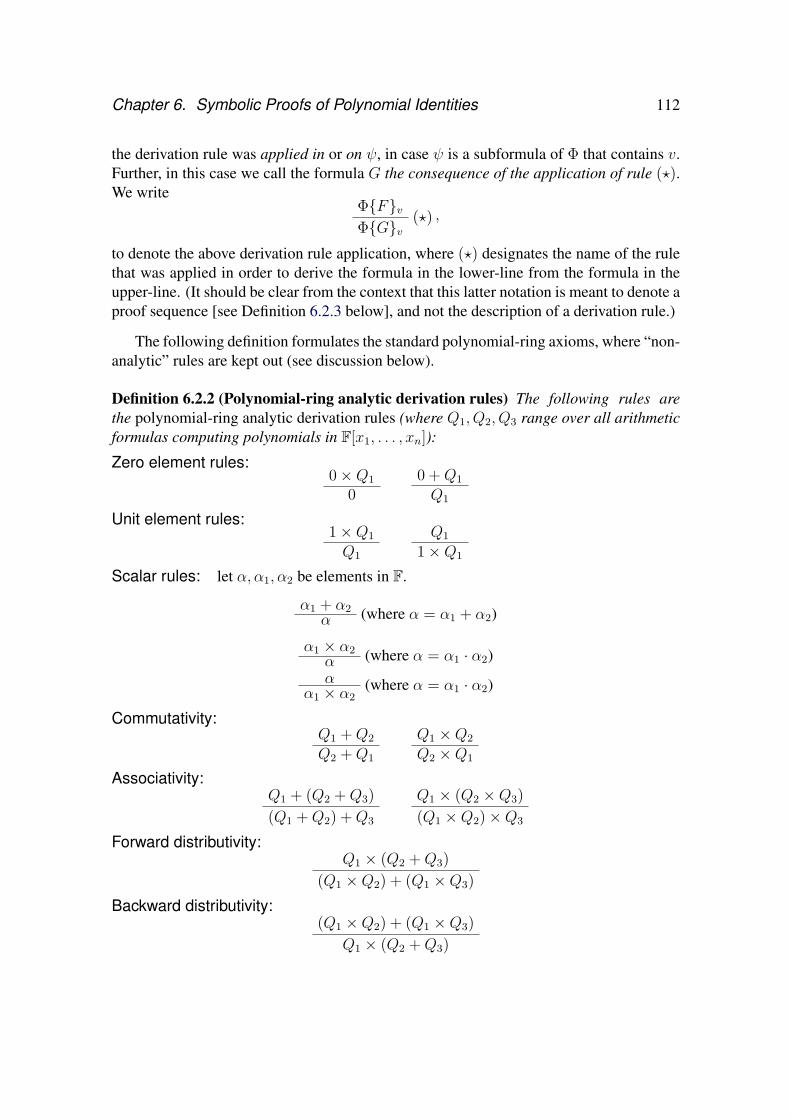
Chapter 6. Symbolic Proofs of Polynomial Identities 112
the derivation rule was applied in or on ψ, in case ψ is a subformula of Φ that contains v.Further, in this case we call the formula G the consequence of the application of rule (?).We write
ΦFv(?)
ΦGv,
to denote the above derivation rule application, where (?) designates the name of the rulethat was applied in order to derive the formula in the lower-line from the formula in theupper-line. (It should be clear from the context that this latter notation is meant to denote aproof sequence [see Definition 6.2.3 below], and not the description of a derivation rule.)
The following definition formulates the standard polynomial-ring axioms, where “non-analytic” rules are kept out (see discussion below).
Definition 6.2.2 (Polynomial-ring analytic derivation rules) The following rules arethe polynomial-ring analytic derivation rules (where Q1, Q2, Q3 range over all arithmeticformulas computing polynomials in F[x1, . . . , xn]):
Zero element rules:0×Q1
00 +Q1
Q1
Unit element rules:1×Q1
Q1
Q1
1×Q1
Scalar rules: let α, α1, α2 be elements in F.
α1 + α2 (where α = α1 + α2)α
α1 × α2 (where α = α1 · α2)αα (where α = α1 · α2)
α1 × α2
Commutativity:Q1 +Q2
Q2 +Q1
Q1 ×Q2
Q2 ×Q1
Associativity:Q1 + (Q2 +Q3)
(Q1 +Q2) +Q3
Q1 × (Q2 ×Q3)
(Q1 ×Q2)×Q3
Forward distributivity:Q1 × (Q2 +Q3)
(Q1 ×Q2) + (Q1 ×Q3)
Backward distributivity:(Q1 ×Q2) + (Q1 ×Q3)
Q1 × (Q2 +Q3)

Chapter 6. Symbolic Proofs of Polynomial Identities 113
Comment: It is easy to show that by using the commutativity and associativity (to the left)rules in Definition 6.2.2, one can efficiently simulate the associativity to the right rules.
Definition 6.2.3 (Analytic symbolic proofs of polynomial identities) Let Φ and Φ′ betwo arithmetic formulas (computing the same polynomial in F[x1, . . . , xn]). An analyticsymbolic derivation of Φ′ from Φ is a sequence of arithmetic formulas ψ1, . . . , ψm suchthat ψ1 ≡ Φ, ψm ≡ Φ′, and for all 1 < i ≤ m, ψi is derived from ψi−1 by applying thepolynomial-ring analytic derivation-rules (applicable on any subformula) from Definition6.2.2. If the initial formula Φ computes the zero polynomial and Φ′ is the formula 0, thenwe call such a derivation of Φ′ from Φ an analytic symbolic proof of Φ.
The length of an analytic symbolic proof (or derivation) is defined to be the numberof proof-lines in the proof (derivation, respectively).
We shall prove the completeness (and soundness) of analytic symbolic proofs in Sec-tion 6.4.
Discussion about analytic symbolic proofs and the subformula property. Let us ex-plain our choice of derivation rules in Definition 6.2.2. Recall from the introductory chap-ter (Section 1.2.3.3) that we aim at formulating analytic symbolic proofs, that is, a systemthat enjoys a sort of subformula property. The intuitive interpretation of this property inour setting would be to prevent the prover from using “clever tricks” (or “detours”) whenproving polynomial identities, in the sense that one cannot introduce new algebraic formu-las that might help in efficiently proving the identities (like, introducing new monomialsor new formulas, later to be cut-off in the proof).
The subformula property usually states that every formula that appears in an analyticproof sequence π of T also appears in the terminal proof-line T . In our setting this shouldmean that the consequence (i.e., lower-line) in any rule may only contain subformulasalready appearing in the premise (i.e., upper-line) of the rule. (Note that in a standardsequent calculus proof, the proof starts with the axioms and terminates in a tautology; thisshould be analogous, in our setting, to a symbolic proofs of an arithmetic formula com-puting the zero polynomial taken backward: one starts from the “axiom” formula 0 anddevelops the formula computing the zero-polynomial; thus, whereas the subformula crite-rion usually requires that every formula in an upper-line of a rule occurs as a subformulain the lower-line of the rule, we should require that every (sub)formula in a lower-line of arule should appear in some sense in the upper-line of the rule.) However, in our system wecannot follow precisely this requirement, since the two distributivity rules might changethe structure of subformulas (for instance, (Q1 × Q2) in the lower-line of the forwarddistributivity rule is not a subformula of the upper-line Q1 × (Q2 + Q3)). Nevertheless,analytic symbolic proofs keep a relaxed subformula property (a “sub-monomial property”,so to speak), as we now explain.
We say that a monomial is syntactically computed by an arithmetic formula Φ if itoccurs in the set of monomials that results when expanding all the monomials in Φ whileusing no canceling of monomials (no canceling of monomials occurs also in any gate

Chapter 6. Symbolic Proofs of Polynomial Identities 114
of Φ, not just the root gate).2 In analytic symbolic proofs we have the following “sub-monomial property”: If π is an analytic symbolic proof and the formula Φ is a proof-line(not a proper subformula in a proof-line) in π, then every monomial that is syntacticallycomputed by Φ either is syntactically computed by the initial proof-line (again, not aproper subformula of the initial proof-line), or is the sum of (two or more) monomials thatare syntactically computed in the initial proof-line. This way, the number of monomialssyntactically computed by each proof-line does not increase along the proof sequence. Weshall not prove this statement formally here, and so this idea should only be kept as anintuition in the mind of the reader.
Consider the following three (sound) derivation rules (absent from our system):
(i) Q1
Q1 + 0; (ii) 0
0×Q1; (iii) α
α1 + α2(where α = α1 +α2, for α1, α2, α ∈ F).
We explain now how the choice not to include the above three rules helps us in keepingthe relaxed form of the subformula property in our proof system. First, given Φ, one cannotsimply derive Φ + ∆−∆ from Φ, where ∆ is any non-empty formula. Note that for thisderivation to be possible, we would need the following derivation sequence that uses rules(i) and (ii) above:
Φ apply rule (i)Φ + 0 apply rule (ii)
Φ + 0×∆Φ + (1− 1)×∆
Φ + 1×∆ + (−1)×∆
Φ + ∆ + (−1)×∆ .
Second, if we had the rule (iii) in our proof system it would be possible to add arbitrarynumber of new monomials that are syntactically computed by proof-lines throughout theproof, as the following example illustrates:
3× (x1 × x2)apply rule (iii)
(2 + 1)× (x1 × x2)
2× (x1 × x2) + 1× (x1 × x2). . .
6.2.1 Depth-3 formulas and depth-3 analytic symbolic proofs
We now consider analytic symbolic proofs of polynomial identities operating with depth-3arithmetic formulas. The standard definition of depth-3 (and specifically ΣΠΣ) arithmeticformulas includes all formulas that can be written as a sum of products of linear poly-nomials. In other words, according to the standard definition, a ΣΠΣ formula Φ (in the
2A monomial here means a product of variables with its scalar coefficient.
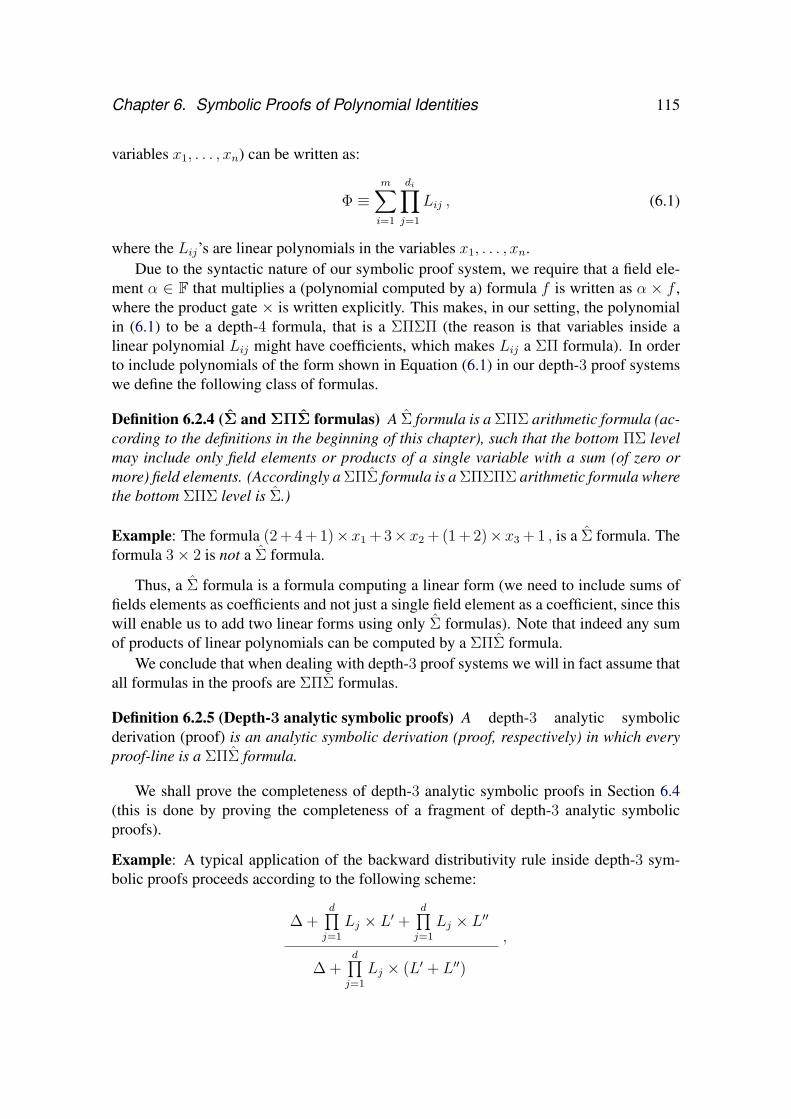
Chapter 6. Symbolic Proofs of Polynomial Identities 115
variables x1, . . . , xn) can be written as:
Φ ≡m∑i=1
di∏j=1
Lij , (6.1)
where the Lij’s are linear polynomials in the variables x1, . . . , xn.Due to the syntactic nature of our symbolic proof system, we require that a field ele-
ment α ∈ F that multiplies a (polynomial computed by a) formula f is written as α × f ,where the product gate × is written explicitly. This makes, in our setting, the polynomialin (6.1) to be a depth-4 formula, that is a ΣΠΣΠ (the reason is that variables inside alinear polynomial Lij might have coefficients, which makes Lij a ΣΠ formula). In orderto include polynomials of the form shown in Equation (6.1) in our depth-3 proof systemswe define the following class of formulas.
Definition 6.2.4 (Σ and ΣΠΣ formulas) A Σ formula is a ΣΠΣ arithmetic formula (ac-cording to the definitions in the beginning of this chapter), such that the bottom ΠΣ levelmay include only field elements or products of a single variable with a sum (of zero ormore) field elements. (Accordingly a ΣΠΣ formula is a ΣΠΣΠΣ arithmetic formula wherethe bottom ΣΠΣ level is Σ.)
Example: The formula (2 + 4 + 1)× x1 + 3× x2 + (1 + 2)× x3 + 1 , is a Σ formula. Theformula 3× 2 is not a Σ formula.
Thus, a Σ formula is a formula computing a linear form (we need to include sums offields elements as coefficients and not just a single field element as a coefficient, since thiswill enable us to add two linear forms using only Σ formulas). Note that indeed any sumof products of linear polynomials can be computed by a ΣΠΣ formula.
We conclude that when dealing with depth-3 proof systems we will in fact assume thatall formulas in the proofs are ΣΠΣ formulas.
Definition 6.2.5 (Depth-3 analytic symbolic proofs) A depth-3 analytic symbolicderivation (proof) is an analytic symbolic derivation (proof, respectively) in which everyproof-line is a ΣΠΣ formula.
We shall prove the completeness of depth-3 analytic symbolic proofs in Section 6.4(this is done by proving the completeness of a fragment of depth-3 analytic symbolicproofs).
Example: A typical application of the backward distributivity rule inside depth-3 sym-bolic proofs proceeds according to the following scheme:
∆ +d∏j=1
Lj × L′ +d∏j=1
Lj × L′′
∆ +d∏j=1
Lj × (L′ + L′′)
,

Chapter 6. Symbolic Proofs of Polynomial Identities 116
where L′, L′′ and the Lj’s are formulas of linear polynomials in the variables x1, . . . , xnand ∆ is any possibly empty formula (note that the two occurrences of
∏dj=1 Lj in the
upper-line must be identical).(When exchanging the upper- and lower- lines, we get a typical application of the
forward distributivity rule.)
6.3 The Structure of Symbolic ProofsIn this section we develop terminology and concepts for dealing with structural propertiesof symbolic proofs. The notions developed here are suitable mainly for dealing withsmall depth symbolic proofs, as the notions mainly take into account the top gates of theformulas in the proofs. This will suffice for stating and proving our main lower bounds.
We will identify a certain graph structure induced by symbolic proofs. The idea isto partition the graph into levels, each level corresponds to a proof-line. Each node inlevel i corresponds to one summand of the formula in the ith line of the proof. From eachsummand (that is, a vertex in the graph) there will be edge(s) directed to its “immediateancestor(s)” in the previous line. The formal definition follows.
Definition 6.3.1 (Underlying graph of analytic symbolic proof) Let π = (Φ1, . . . ,Φm)be an analytic symbolic proof. Define the underlying directed acyclic graph of π denotedGπ as follows. The graph Gπ has m levels and edges may only go from level i to leveli− 1, for 1 < i ≤ m (the vertices in level 1 have no outgoing edges). For any 1 ≤ i ≤ m,write Φi as ϕ1 + . . .+ϕ`i , for some `i ≥ 1, where every ϕj is either a product formula or aformula containing only a single leaf. Then, the ith level ofGπ consists of `i vertices, eachvertex is labeled by a different summand ϕj from Φi and if 1 ≤ i < m then the incomingedges of level i (from vertices in level i + 1) are defined as follows (we shall sometimeabuse notation by identifying a vertex in the graph Gπ with its label and a level in thegraph Gπ with its corresponding proof-line in π):
(i) In case no rule was applied on ϕj in level i, for j ∈ [`i] (see notation after Definition6.2.1), then ϕj appears (as a single vertex) in both level i and level i+ 1, and we putan incoming edge from ϕj in level i+ 1 to ϕj in level i.
(ii) Assume that a rule different from the forward distributivity rule was applied on ϕjin level i, for j ∈ [`i]. Since ϕj is in a separate vertex in Gπ and some rule wasapplied on ϕj (in the ith step in π) then it must be that ϕj is a product formula (andnot a single leaf formula). It can be verified by a straightforward inspection of thederivation rules (Definition 6.2.2) that a consequence of any rule different from theforward distributivity rule is not a plus formulas, and so the consequence of ϕj inproof-line i + 1 in π is (still) a product formula. This implies that there is a singlevertex ϕ′j in level i + 1 which is the consequence of ϕj . We define ϕj in level i tohave a single incoming edged from ϕ′j in level i+ 1.
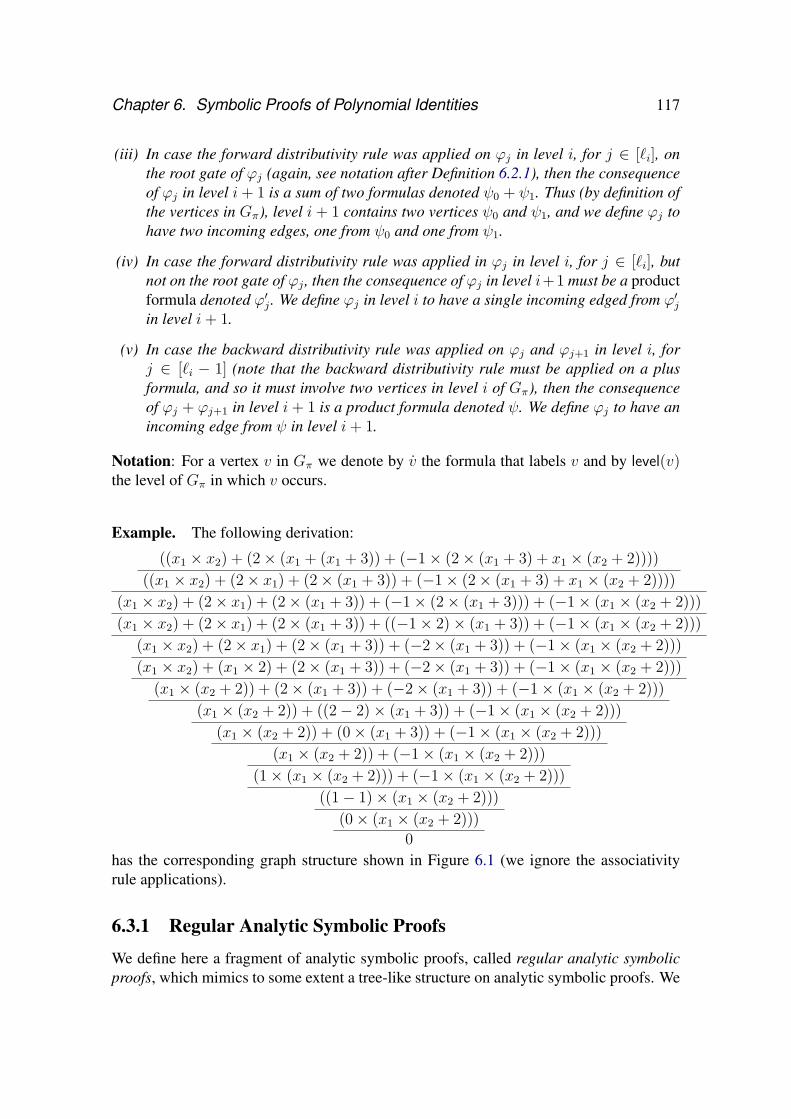
Chapter 6. Symbolic Proofs of Polynomial Identities 117
(iii) In case the forward distributivity rule was applied on ϕj in level i, for j ∈ [`i], onthe root gate of ϕj (again, see notation after Definition 6.2.1), then the consequenceof ϕj in level i+ 1 is a sum of two formulas denoted ψ0 + ψ1. Thus (by definition ofthe vertices in Gπ), level i + 1 contains two vertices ψ0 and ψ1, and we define ϕj tohave two incoming edges, one from ψ0 and one from ψ1.
(iv) In case the forward distributivity rule was applied in ϕj in level i, for j ∈ [`i], butnot on the root gate of ϕj , then the consequence of ϕj in level i+1 must be a productformula denoted ϕ′j . We define ϕj in level i to have a single incoming edged from ϕ′jin level i+ 1.
(v) In case the backward distributivity rule was applied on ϕj and ϕj+1 in level i, forj ∈ [`i − 1] (note that the backward distributivity rule must be applied on a plusformula, and so it must involve two vertices in level i of Gπ), then the consequenceof ϕj + ϕj+1 in level i + 1 is a product formula denoted ψ. We define ϕj to have anincoming edge from ψ in level i+ 1.
Notation: For a vertex v in Gπ we denote by v the formula that labels v and by level(v)the level of Gπ in which v occurs.
Example. The following derivation:
((x1 × x2) + (2× (x1 + (x1 + 3)) + (−1× (2× (x1 + 3) + x1 × (x2 + 2))))
((x1 × x2) + (2× x1) + (2× (x1 + 3)) + (−1× (2× (x1 + 3) + x1 × (x2 + 2))))
(x1 × x2) + (2× x1) + (2× (x1 + 3)) + (−1× (2× (x1 + 3))) + (−1× (x1 × (x2 + 2)))
(x1 × x2) + (2× x1) + (2× (x1 + 3)) + ((−1× 2)× (x1 + 3)) + (−1× (x1 × (x2 + 2)))
(x1 × x2) + (2× x1) + (2× (x1 + 3)) + (−2× (x1 + 3)) + (−1× (x1 × (x2 + 2)))
(x1 × x2) + (x1 × 2) + (2× (x1 + 3)) + (−2× (x1 + 3)) + (−1× (x1 × (x2 + 2)))
(x1 × (x2 + 2)) + (2× (x1 + 3)) + (−2× (x1 + 3)) + (−1× (x1 × (x2 + 2)))
(x1 × (x2 + 2)) + ((2− 2)× (x1 + 3)) + (−1× (x1 × (x2 + 2)))
(x1 × (x2 + 2)) + (0× (x1 + 3)) + (−1× (x1 × (x2 + 2)))
(x1 × (x2 + 2)) + (−1× (x1 × (x2 + 2)))
(1× (x1 × (x2 + 2))) + (−1× (x1 × (x2 + 2)))
((1− 1)× (x1 × (x2 + 2)))
(0× (x1 × (x2 + 2)))
0
has the corresponding graph structure shown in Figure 6.1 (we ignore the associativityrule applications).
6.3.1 Regular Analytic Symbolic Proofs
We define here a fragment of analytic symbolic proofs, called regular analytic symbolicproofs, which mimics to some extent a tree-like structure on analytic symbolic proofs. We

Chapter 6. Symbolic Proofs of Polynomial Identities 118
(x1 × x2)
(x1 × x2)
(x1 × x2)
(x1 × x2)
(x1 × x2)
(2× (x1 + (x1 + 3)))
(2× (x1 + 3))
(x1 × 2)
(2× (x1 + 3))(2× x1)
(2× (x1 + 3))(2× x1)
(2× (x1 + 3))(2× (x1 + 3))(2× x1)
(2× (x1 + 3))(2× x1)
(−1× (2× (x1 + 3) + x1 × (x2 + 2)))
(−1× (x1 × (x2 + 2)))(−1× (2× (x1 + 3)))
(−1× (x1 × (x2 + 2)))
(−1× (2× (x1 + 3) + x1 × (x2 + 2)))
(−1× (x1 × (x2 + 2)))((−1× 2)× (x1 + 3))
(−2× (x1 + 3)) (−1× (x1 × (x2 + 2)))(−2× (x1 + 3))
(x1 × x2) (2× (x1 + 3)) (−1× (x1 × (x2 + 2)))(−2× (x1 + 3))
(−1× (x1 × (x2 + 2)))(−2× (x1 + 3))(x1 × (x2 + 2))
(−1× (x1 × (x2 + 2)))((2− 2)× (x1 + 3))(x1 × (x2 + 2))
(−1× (x1 × (x2 + 2)))(0× (x1 + 3))(x1 × (x2 + 2))
(−1× (x1 × (x2 + 2)))0(x1 × (x2 + 2))
(−1× (x1 × (x2 + 2)))(x1 × (x2 + 2))
(1× (x1 × (x2 + 2))) (−1× (x1 × (x2 + 2)))
0
((1− 1)× (x1 × (x2 + 2)))
(0× (x1 × (x2 + 2)))
Figure 6.1: Underlying graph of an analytic symbolic proof (this proof is also regular [seeDefinition 6.3.4]). A single shaded vertex in a level means that a derivation rule is applied on thisvertex (that is, an application rule is applied on one of the gates [formally, nodes] in the formulalabeling the vertex). Two shaded vertices in a level means that the backward distributivity rule isapplied in π on the plus gate (in the corresponding proof-line in π) that has the two shaded verticesas its children.
shall use the following two definitions for that purpose.Atomic formulas are essentially formulas computing single monomials:
Definition 6.3.2 (Atomic and non-atomic formulas) A formula Φ is atomic if it has theform φ1 × · · · × φk, for k ≥ 1, where each φi (1 ≤ i ≤ k) is either a variable or a sum ofone or more field elements; otherwise, Φ is said to be non-atomic.
Example: The formulas (1 + 2)× x2× x1 and 1× 3× x1 are atomic formulas, as well asthe formula 0 and the formula x1. The formula x2 + 3 is a non-atomic formula.
Definition 6.3.3 Given a proof π and its underlying graph Gπ let G′ be the subgraph ofGπ induced by considering only the non-atomic vertices in Gπ, and let v be a vertex in G′.Then, Tv(Gπ) is defined to be the directed subgraph of G′ induced by all the vertices (inG′) reachable from v via a directed-path in G′ (including v itself).
The idea of the regularity condition of analytic symbolic proofs we are about to defineis to guarantee that if a forward distribution rule is applied on A× (B +C), which breaksthe formula into the sum of two terms A×B andA×C , then the two formulasA×B and

Chapter 6. Symbolic Proofs of Polynomial Identities 119
A×C, as well as any other two formulas that originate from A×B and A×C (possiblyalso originating by other formulas), might not be united together again by means of thebackward distributivity rule (in fact, this rule is the only rule that can “unite” two separatesummands into a product formula) .
In the terminology of the graph structure of analytic symbolic proofs (Definition 6.3.1)the regularity condition means that a vertex v in a proof-graph cannot have two edge-disjoint (directed) paths starting in v and leading to the same vertex.
Definition 6.3.4 (Regular analytic symbolic proofs) Let π be an analytic symbolicproof. We say that π is a regular analytic symbolic proof (or regular proof for short),if for every (non-atomic) vertex v in Gπ, the subgraph Tv(Gπ) is a tree.3
In other words, analytic symbolic proofs are regular if for every (non-atomic) vertexw in their underlying proof-graph there are no two distinct directed paths originating in wthat reach a common vertex (different from w).
Example: Figure 6.1 illustrates a regular analytic symbolic proof. One can verify that forevery (non-atomic) vertex w in the graph there are no two distinct directed paths originat-ing in w that reach a common vertex.
Comment: In the definition of regular proofs we need to specifically refer to non-atomicvertices (through the definition of Tv(Gπ)) for the following reason. If for no vertex vin Gπ does one get by two distinct (directed) paths from v to a vertex correspondingto an initial summand (in the initial formula), then some formulas computing the zeropolynomial might not be provable. Consider for example the formula (x1 + 1) × (x1 −1)−x1×x1−1. This formula computes the zero polynomial. However, the first term (fromthe left) is a product formula that when expanded, contains the two canceling monomialsx1 × −1 and 1 × x1. Thus, in order to reach the formula 0 we must enable these twoterms to cancel each other (that is, to derive the (sub-)formula 0 from them). Hence, thisamounts to a vertex labeled ((1− 1)×x1) in Gπ from which two distinct paths lead to thesame initial summand (x1 + 1)× (x1 − 1).
We use the following simple structural proposition in the next sections. Essentially,the proposition states that if there is a derivation starting with ∆ + Θ and terminates in∆′ + ϕ, and ϕ in the terminal line was “originated” only from Θ in the initial line, thenthere is a derivation starting in Θ and terminating in ∆′′ + ϕ for some possibly emptyformula ∆′′.
Proposition 6.3.5 Let Θ and ∆ be two formulas, and assume that ϕ is a product formula(or a single leaf formula) such that there is a regular analytic symbolic derivation π start-ing from ∆ + Θ and deriving ∆′ + ϕ, where ∆′ is any possibly empty formula. Denote byGπ the underlying graph of π, and let v be the vertex in the maximal level of Gπ that islabeled with ϕ. Let T be the set of vertices of Tv(Gπ), let A be the set of all the vertices
3The intention here, of course, is that Tv(Gπ) is a tree also when considered as an undirected graph, thatis, when replacing every directed edge in Tv(Gπ) with an undirected one.

Chapter 6. Symbolic Proofs of Polynomial Identities 120
in level 1 of Gπ, and let B be the set of all the vertices that are labeled with summandsof Θ in the first level of Gπ. If (T ∩A) ⊆ B , then there is a regular analytic symbolicderivation π′ starting from Θ alone and deriving ∆′′ + ϕ, where ∆′′ is any possibly emptyformula.
Proof. Starting from Tv(Gπ), we construct a new graph G′ that is a legitimate underlyinggraph of a regular analytic symbolic proof of ∆′′ + ϕ, where ∆′′ is any possibly emptyformula (we ignore the order of additions).
Let G′ := Tv(Gπ).Step I: For every u ∈ B\T, we add to every level 1 ≤ j ≤ level(v) in4 G′ a new copy
of u, and put an edge from u in level j to u in level (j − 1) in G′ (for 1 < j ≤ level(v)).Step II: For all vertices w in Tv(Gπ) such that w 6= v, we do the following. Let
` = level(w). By definition of Tv(Gπ) there is a vertex u ∈ T such that w has an incomingedge from u in Tv(Gπ) (since there is a directed path from v to w in Tv(Gπ)). Assumethat there is a vertex r ∈ Gπ \T such that w has an incoming edge from r. Then,
(i) we add the vertex r to level `+ 1 in G′; and(ii) we add an edge from r to w in G′; and(iii) we add to every level j > ` + 1 in G′ a new copy of r, and put an edge from r in
level j to r in level (j − 1) in G′.
We claim that G′ is the underlying graph of a regular analytic symbolic derivationstarting from Θ and deriving ∆′′ + ϕ, for some possibly empty formula ∆′′. Note thatthe first level of G′ consists precisely of the summands of Θ, and that the last level of G′
contains the vertex v. Moreover, G′ conforms to the regularity conditions: no vertex in G′
has two distinct (non trivial) directed paths that reach the same vertex in G′.Thus, we only need to show that G′ constitutes a legal analytic symbolic derivation.
To this end, it suffices to show that every level j > 1 in G′ corresponds to a proof-line thatis derivable from the previous level j− 1, and that the edges from vertices in level j to thevertices in level j − 1 in G′ are legal (that is, conform to the definition of an underlyinggraph of an analytic symbolic proof):
Let w be a vertex in level j > 1 in G′, and consider the following cases:
1. If w 6∈ T and w was added in Step I to G′, then w was added to G′ along with asingle outgoing edge that points into another copy of w in level j − 1 in G′, and sowe are done.
2. If w ∈ T, then, by definition, there is an edge from w to another vertex u ∈ T andhence u is in G′. In case u has fan-in 1 in Gπ we are done.
Otherwise, there is a (unique) vertex r 6= w in Gπ such that r has an edge e pointingto u in Gπ. By the construction of G′ (Step II, items (i) and (ii) above), both r andthe edge e are in G′, and so both w and r and their outgoing edges correspond to alegal derivation. This takes care of all the vertices in level j in G′ that are not in T,as well as all the vertices r added to G′ in level j, in Step II, item (i) above.
4Clearly, every vertex in Tv(Gπ) retain the same level it had in Gπ .

Chapter 6. Symbolic Proofs of Polynomial Identities 121
3. If w 6∈ T and w was added to G′ in Step II, item (iii) above, then w has a singleoutgoing edge that points to a copy of w in level j − 1 of G′, and we are done.
Comment: By inspecting the proof of Proposition 6.3.5, it is evident that the statementof this proposition also holds for regular analytic symbolic proofs operating with depth-3formulas. We shall use this fact in the sequel.
6.4 CompletenessRecall that when dealing with depth-3 formulas computing the zero polynomial, we as-sume that the formulas are in fact ΣΠΣ formulas (Definition 6.2.4).
Theorem 6.4.1 (Completeness of regular analytic depth-3 symbolic proofs) Regularanalytic depth-3 symbolic proofs are complete in the sense that every depth-3 formulacomputing the zero polynomial has such a proof; and sound in the sense that onlyformulas computing the zero polynomial have such proofs.
Proof sketch: Soundness stems from the soundness of the derivation rules: every derivationrule that is applied on some formula Φ yields a formula computing the same polynomialas Φ. We turn to proving completeness.
We first expand all the (formulas of) monomials (including their coefficients, and withno cancelations applied anywhere) in each summand in the initial ΣΠΣ formula. This steprequires only the successive application of the forward distributivity rule. In particular,assume that Φ ≡ ψ1 + . . . + ψk, for some k ≥ 1, is a ΣΠΣ formula computing the zeropolynomial, where each ψi is a ΠΣ formula. Then, applying the forward distributivity ruleon the root product gate of a summand ψi (for i ∈ [k]), yields a new ΣΠΣ formula.
Next we derive the 0 formula from every group of canceling monomials. Thus, wearrive at a sum of 0’s formulas. This can be further reduced into a single 0 by the zeroelement rule.
By simple inspection of the underlying graph of the above proof it is easy to see that thegraph obtained is regular: Every non-atomic vertex has only a single (directed) path thatends at the vertex labeled with a summand from the initial line. Thus, every non-atomicvertex v trivially induces a tree, via Tv(Gπ), in the underlying graph, which preciselymeans that the proof is regular.
In the same manner we can get the completeness and soundness properties for unre-stricted depth regular symbolic proofs for the set of all formulas that compute the zeropolynomial.
Theorem 6.4.2 Analytic symbolic proofs are sound and complete for the set of formulascomputing the zero polynomial.

Chapter 6. Symbolic Proofs of Polynomial Identities 122
Proof. Soundness stems from the soundness of the derivation rules. For completeness,we first expand all the (formulas of) monomials (including their coefficients, and withno cancelations applied anywhere) in each summand in the initial formula (and withouttaking care for the depth of formulas). Then we proceed as in the proof of Theorem 6.4.1.
6.5 Lower BoundsIn this section we demonstrate exponential-size lower bounds on the length of regularanalytic symbolic proofs operating with depth-3 formulas of certain polynomial identi-ties. The hard instances will be built from small depth-3 formulas that we already met inprevious chapters, that is, formulas for the elementary symmetric polynomials over largeenough fields.
6.5.1 Hard Formulas
We shall consider from now on all arithmetic formulas to compute polynomials over thefield of complex numbers C. The following depth-3 formula will serve as our hard in-stance.
Symn :≡ r0 × (x1 + b0)× (x2 + b0)×· · · × (xn + b0) +
r1 × (x1 + b1)× (x2 + b1)×· · · × (xn + b1) +
· · · (6.2)rn × (x1 + bn)× (x2 + bn)×· · · × (xn + bn) −1 ,
where r0, . . . , rn are some n + 1 complex numbers and b0, b1, . . . , bn are n + 1 distinctnon-zero complex numbers (each of which is different from 1).
The jth summand in Symn, for 0 ≤ j ≤ n, is a ΠΣ formula (and hence specifically aΠΣ formula) and is denoted An,j . In other words,
An,j ≡ rj × (x1 + bj)× (x2 + bj)× . . .× (xn + bj) , (6.3)
and so
Symn ≡n∑j=0
An,j − 1 .
Proposition 6.5.1 There exist complex numbers r0, . . . , rn and n + 1 distinct nonzerocomplex numbers b0, . . . , bn (each of which is different from 1), so that Symn computesthe zero polynomial.

Chapter 6. Symbolic Proofs of Polynomial Identities 123
Proof. Consider the polynomial 1 as the symmetric multilinear polynomial of degree0. By Theorem 2.5.4 in the preliminaries (Chapter 2, Section 2.5.4), there is a depth-3multilinear arithmetic formula Φ with a plus gate at the root computing 1 where Φ has aspecial form: specifically, by Equation 2.4 in the proof of Theorem 2.5.4, this formula Φcan be written as:
n∑j=0
rj ·n∏i=1
(xi + bj) ,
for any chosen distinct bj’s complex numbers. (Also notice that there must be at least onenonzero ri (0 ≤ i ≤ n).)
6.5.2 Key Lemma: Lower Bounds on Deriving One Formula fromAnother
In this subsection we show a lower bound on the length of regular analytic symbolicderivations operating with ΣΠΣ formulas needed to derive a certain formula from anotherformula. Specifically, we provide two formulas Φ and Ψ, such that starting from Φ onecannot efficiently derive any formula that contains Ψ as a subformula. This will thenfacilitate us in the next subsection (when proving lower bounds on the length of proofs offormulas computing the zero polynomial, that is, on the derivation length needed to reachthe formula 0). Note that the task of deriving a certain formula from a different formula,and the task of proving that a formula computes the zero polynomial (by deriving thezero formula) are not necessarily identical tasks since our derivation rules are asymmetric(Definition 6.2.2).5
We work in depth-3 from now on, and specifically with ΣΠΣ formulas.
Definition 6.5.2 (Derivable subformulas) Let Φ be a formula. The collection of all for-mulas Ψ for which there is an analytic symbolic derivation of Ψ from Φ are said to bethe formulas derivable from Φ. If B is the set of all formulas derivable from Φ then theset of all subformulas of formulas in B is called the set of subformulas derivable from Φ,denoted deriv(Φ).
Example: Let Φ be the Σ formula (xi + b1). Then, the derivable formulas from Φ are,e.g., (xi + b1), (b1 +xi) and all Σ formulas
∏i∈I cj ×
(∏k∈K aj × xi +
∏j∈J bj
), where∏
i∈I ci =∏
k∈K ak = 1 and∏
j∈J bj = b1. Note that (xi + b2 + b3) is not derivable from(xi + b1), even when b2 + b3 = b1 is true in the field; this stems from the definition ofour derivation rules (Definition 6.2.2). Further, xi, b1 and (xi + b1), for instance, are in
5To see this, observe that deriving ψ1 from ψ2 means that we can derive ψ1 − ψ1 from ψ2 − ψ1, andthus we can derive 0 from ψ2 −ψ1. On the other hand, deriving 0 from ψ2 −ψ1 does not imply that we canderive ψ1 from ψ2 (note that we cannot start from ψ2, add −ψ1 +ψ1 to yield ψ2−ψ1 +ψ1, and then derive0 from the first two summands to yield ψ1; this is because we would need a rule to introduce the formula−ψ1 + ψ1 in the first step, and we do not have such a rule in analytic symbolic proofs).

Chapter 6. Symbolic Proofs of Polynomial Identities 124
derive(xi + b1), while (xi + b0) 6∈ derive(xi + b1) (in case b0 6= b1) (see Proposition 6.5.9for a proof).
The following definition is basically the transitive closure of a formula under “for-ward” and “backward” applications of all rules excluding the two distributivity rules (un-less the distributivity rules are applied inside Σ formulas).
Definition 6.5.3 (Simple descendants and simple ancestors) Given a formula Ψ we de-fine Cl(Ψ) as the smallest set of formulas containing Ψ and satisfying the following: As-sume that ∆ is a formula and v is some node in the (tree of) ∆, then:
(i) If ∆φ+ 0v ∈ Cl(Ψ), then ∆φv ∈ Cl(Ψ) ;
(ii) If ∆α1 + α2v ∈ Cl(Ψ), then ∆αv ∈ Cl(Ψ) for α, α1, α2 ∈ F, such that α =α1 + α2 ;
(iii) ∆φ× 1v ∈ Cl(Ψ) iff ∆φv ∈ Cl(Ψ) ;
(iv) ∆α1×α2v ∈ Cl(Ψ) iff ∆αv ∈ Cl(Ψ) , for α, α1, α2 ∈ F such that α = α1×α2 ;
(v) ∆φ2 φ1v ∈ Cl(Ψ) iff ∆φ1 φ2v ∈ Cl(Ψ) , where ∈ +,×;
(vi) ∆(φ1 φ2) φ3v ∈ Cl(Ψ) iff ∆φ1 (φ2 φ3)v ∈ Cl(Ψ) , where ∈ +,×;
(vii) ∆(∑
j∈J αj +∑
k∈K αk
)× xi
v∈ Cl(Ψ) (where |J |, |K| ≥ 1 and for all j ∈ J
and k ∈ K, αj, αk ∈ F ) iff ∆
(∑
j∈J αj)× xi +(∑
k∈K αk)× xi
v∈ Cl(Ψ) ;
(viii) ∆(∑
j∈J αj
)× (xi + xj)
v∈ Cl(Ψ) iff
∆(∑
j∈J αj
)× xi +
(∑j∈J αj
)× xj
v
, where αj ∈ F (for all j ∈ J) and
|J | ≥ 1.
Whenever Ψ′ ∈ Cl(Ψ) we call Ψ′ a simple descendant of Ψ , and Ψ a simple ancestor ofΨ′. Given a formula Ψ we denote by Cl−(Ψ) the set of all simple ancestors of Ψ, that is,the set of all Φ such that Ψ ∈ Cl(Φ).
Note: Observe that Cl−(Ψ) is closed under the specified derivation rules when they areapplied “backward” on the formulas in Cl−(Ψ). Also note that the only items in Definition6.5.3 that are asymmetric are items (i) and (ii).
Comment: The last two clauses (vii) and (viii) in Definition 6.5.3 intend to deal with dis-tributivity rules applied inside Σ formulas only (and those distributivity rule applicationswhose consequence is a Σ formula).

Chapter 6. Symbolic Proofs of Polynomial Identities 125
We shall use the following abbreviation (this is identical to Symn when excluding thefirst summand An,0).
Initn :≡ r1 × (x1 + b1)× (x2 + b1)× · · · × (xn + b1) +
r2 × (x1 + b2)× (x2 + b2)× · · · × (xn + b2) +
· · · (6.4)rn × (x1 + bn)× (x2 + bn)× · · · × (xn + bn)
−1 .
We thus have, by Equation (6.3):
Initn ≡n∑j=1
An,j − 1 . (6.5)
Definition 6.5.4 (Proper Σ formulas) A proper Σ formula is a Σ formula which is a plusformula (that is, it has a plus gate at the root). A proper ΠΣ formula is a proper ΠΣformula where the Σ formulas in the bottom levels are replaced by proper Σ formulas.Similarly, a proper ΣΠΣ formula is a proper ΣΠΣ formula where the Σ formulas in thebottom levels are replaced by proper Σ formulas.
Note that every proper Σ formula (Section 6.1) is a proper Σ formula, while not everyproper Σ formula is a Σ formula.
Lemma 6.5.5 (Key lower bound) Let π be a regular analytic symbolic proof operatingwith ΣΠΣ formulas, and with the initial formula in π being Initn, for some positive n ∈ N.Let Gπ be the corresponding graph of π. Assume that v is a vertex in Gπ labeled with Φ,which is a simple ancestor of
ψ ×m∏k=1
Ψk ,
where ψ is any possibly empty formula, and for every k ∈ [m], i ∈ [n] and j ∈ [n], Ψk isa proper Σ formula, such that Ψk 6∈ deriv(xi + bj). Then |Tv(Gπ)| ≥ 2m.
Proof. We go by induction on m. The idea is to build inductively and in a bottom-upfashion, starting with v, the tree Tv(Gπ), by considering all the possible rules that canderive the formula Φ.
Base case: m = 1. The formula Φ is a simple ancestor of ψ × Ψ1, where ψ is somepossibly empty formula6 and Ψ1 is a proper Σ formula that is not a subformula derivablefrom (xi + bj), for all j ∈ [n] and all i ∈ [n]. Observe that (for any positive n ∈ N) everyproper Σ formula that occurs in Initn has the form (xi + bj), for some j ∈ [n] and i ∈ [n].
6Note that in this case (i.e., when m = 1), since Ψ1 is a proper Σ formula, ψ is in fact a non-emptyformula, as by definition of Gπ , the vertex v cannot be labeled with a plus formula.

Chapter 6. Symbolic Proofs of Polynomial Identities 126
Thus, Φ is different from every subformula in the initial formula Initn, and so the numberof proof-lines in π is at least 2, and we are done.
Induction case: We have that Φ is a simple ancestor of ψ ×∏mk=1 Ψk, where ψ is some
possibly empty formula, m > 1 and the Ψk’s are proper Σ formulas. We shall use thefollowing main technical lemma (whose proof is given in Section 6.5.4).
Lemma 6.5.6 (Technical lemma) If m > 1 then (under the conditions stated in Lemma6.5.5) there exists a vertex y in Tv(Gπ), such that there is a path from v to y in Tv(Gπ),and y has two outgoing edges to two (distinct) vertices u,w, so that: u and w are labeledwith two simple ancestors of the following product formulas
ψ0 ×m−1∏k=1
Ψ′k and ψ1 ×m−1∏k=1
Ψ′′k , (6.6)
respectively, where ψ0, ψ1 are some possibly empty formulas, and for all k ∈ [m − 1],i ∈ [n] and j ∈ [n], Ψ′k,Ψ
′′k are some proper Σ formulas such that Ψ′k 6∈ deriv(xi + bj)
and Ψ′′k 6∈ deriv(xi + bj).
Given Lemma 6.5.6, we can then use the induction hypothesis on the two verticesu,w (whose existence is guaranteed by the lemma), showing that |Tu(Gπ)| ≥ 2k−1 and|Tw(Gπ)| ≥ 2k−1. By the regularity condition we know that Tu(Gπ) and Tw(Gπ) haveno common vertices (note that v is a non-atomic formula [Definition 6.3.2] and so indeedTv(Gπ) is a tree [Definition 6.3.4]). Therefore, |Tv(Gπ)| ≥ |Tu(Gπ)| + |Tw(Gπ)| ≥ 2k,which concludes the proof of Lemma 6.5.5.
In the next section we shall need the following simple generalization of Lemma 6.5.5:
Corollary 6.5.7 Let π be a regular symbolic proof operating with ΣΠΣ formulas, andwith the initial formula in π being ∆+Initn, for some ΣΠΣ formula ∆ and some positiven ∈ N. Let Gπ be the corresponding graph of π. Assume that v is a vertex in Gπ labeledwith Φ, which is a simple ancestor of
ψ ×m∏k=1
Ψk ,
where ψ is any possibly empty formula, and for every k ∈ [m], i ∈ [n] and j ∈ [n], Ψk isa proper Σ formula, such that Ψk 6∈ deriv(xi + bj). Let T be the set of vertices of Tv(Gπ)and let A be the set of all vertices in level 1 of Gπ that are subformulas in ∆ (i.e., thosecorresponding to summands in ∆ in the initial line). If T ∩A = ∅, then |Tv(Gπ)| ≥ 2m.
Proof. Immediate from Lemma 6.5.5 and Proposition 6.3.5.

Chapter 6. Symbolic Proofs of Polynomial Identities 127
6.5.3 Main Lower Bound: Regular Depth-3 Proofs
In this subsection we demonstrate how to use the Key Lemma 6.5.5 in order to prove alower bound on the proof length of Symn, that is, a lower bound on the size of derivationstarting with Symn and terminating with the formula 0.
The main result of this chapter is the following:
Theorem 6.5.8 Every regular analytic symbolic proof operating with ΣΠΣ formulas ofSymn has length 2Ω(n).
Comment: The number of variables in Symn is ` = n · (n + 1), and so Theorem 6.5.8gives a lower bound of 2Ω(
√`).
The rest of this subsection is dedicated to the proof of Theorem 6.5.8. The proofidea goes as follows. We begin by considering the summand An,0 in the first line of π.We expand An,0 by applying the forward distributivity rule as much as we like (withoutusing the backward distributivity rule, but possibly with applying other rules). In casewe expand too much (i.e., exponentially many) summands, we are done. Otherwise, theexpansion of An,0 yields a summand Φ which is a simple ancestor of ψ×∏m
k=1 Ψk , wherem is big enough (that is, m ≥ n/2), and Φ conforms to the conditions in Key Lemma6.5.5 excluding the fact that the initial line of the proof is not necessarily Initn. Since,by assumption, no forward distributivity rule applications are applied on Φ the backwarddistributivity must be applied on it sometime. We can then show that in this case thereexists a vertex v in the underlying graph Gπ of π that fully conforms to the conditionsstated in Key Lemma 6.5.5 (more correctly, v fully conforms to the conditions stated inCorollary 6.5.7), which concludes the lower bound proof.
For every k ∈ [n], we putΨk :≡ (xk + b0) .
Proposition 6.5.9 For all k, i, j ∈ [n], Ψk 6∈ deriv(xi + bj).
Proof. By the definition of the derivation rules (Definition 6.2.2), no rule can increase thenumber of plus gates in a formula, except for the forward distributivity rule
Q1 × (Q2 +Q3)
(Q1 ×Q2) + (Q1 ×Q3):
every plus gate that occurs in (a substitution instance of) Q1 in the upper-line Q1× (Q2 +Q3), appears twice in the lower-line (Q1×Q2) + (Q1×Q3). Note that for this increase inthe number of plus gates to happen, the upper-line Q1 × (Q2 + Q3) must contain at leasttwo plus gates. Thus, if Φ′ is derived from Φ via an analytic symbolic derivation, and Φcontains only one plus gate, then Φ′ contains at most one plus gate. We conclude that forall i, j ∈ [n], any formula derivable from (xi + bj) contains at most one plus gate.
Assume by a way of contradiction that there is a formula ϕ ∈ deriv(xi + bj), such thatthere exists k ∈ [n] for which (xk + b0) occurs inside ϕ. Since ϕ has only one plus gate,

Chapter 6. Symbolic Proofs of Polynomial Identities 128
ϕ ≡ φ × (xk + b0), for some possibly empty formula φ (when ignoring associativity offormulas and the order of multiplication). By the soundness of the proof system, we getthat φ×(xk+b0) and (xi+bj) compute the same polynomial. But, by assumption, bj 6= b0
for all j ∈ [n], and so for all k ∈ [n], (xi + bj) cannot be factored by (xk + b0).
Fix a regular depth-3 analytic symbolic proof π of Symn, and letGπ be the correspond-ing underlying graph of π. Note that the first line of π is Symn ≡ An,0 +Σn
j=1An,j−1, andso the first level of Gπ has a unique vertex labeled with (the product formula) An,0. LetS be the set of all vertices v in Gπ such that v is non-atomic (Definition 6.3.2) and every(directed) path that originates in v terminates in the vertex that is labeled with An,0. Let
T be the subgraph of Gπ induced by the vertices in S .
Proposition 6.5.10 The graph T is a binary tree rooted at An,0 (where every vertex isdirected from leaves toward the root).7
Proof. This stems directly from the regularity condition on the structure of π. Formally,assume by a way of contradiction that there is a (possibly undirected) cycle C in T , andlet u be a vertex in C, where level(u) is the maximal level in Gπ. Since u is in a cycle ithas two edges adjacent to two distinct vertices w, v in C. But then the fan-out of u in Gπ
(considered as a directed graph) is 2, as both v and w must be in a smaller level than thelevel of u (by assumption on the maximality of level(u), and since no two vertices in thesame level of a proof-graph are connected with an edge). Both v and w have a directedpath leading to An,0 in Gπ, and so u has two different paths leading to An,0, in contrastto the regularity condition which forbids this case (since, Tu(Gπ) is a tree, rooted at u).This shows that T is a tree. To show that T is a binary tree, we only need to note that bydefinition, every vertex in Gπ has fan-in at most 2.
Recall the definition of a subformula in a proof-line being the consequence of somederivation rule (Notation after Definition 6.2.1). Also recall that a derivation rule is appliedoutside a subformula ψ if (in the terminology used in Notation after Definition 6.2.1) thevertex v is not in ψ.
Proposition 6.5.11 No vertex in T is (labeled with) a consequence of the backward dis-tributivity rule applied outside a Σ formula.8
Proof. By definition no vertex inGπ is labeled with a plus formula. Hence, all vertices in Tare labeled with (not necessarily proper) ΠΣ formulas (since the proof is restricted to ΣΠΣformulas only). The upper-line in the backward distributivity rule is (Q1×Q2)+(Q1×Q3).
7T is a tree also when considered as an undirected graph.8Here we identify the vertices in T with the corresponding vertices in Gπ (where the latter correspond,
as always, to subformulas occurring in π).

Chapter 6. Symbolic Proofs of Polynomial Identities 129
Assume, by a way of contradiction, that there is a vertex v in T , such that v is aconsequence of the backward distributivity rule applied on (a substitution instance of)(Q1×Q2) + (Q1×Q3) and (Q1×Q2) + (Q1×Q3) is not a Σ formula. In case (Q1×Q2)and (Q1 × Q3) appear in two distinct vertices u,w in Gπ, then we get that v has twooutgoing edges pointing to u and w. By the definition of T , this means that both u and whave directed paths reaching the root of T , which contradicts the regularity condition.
Otherwise, (Q1 ×Q2) + (Q1 ×Q3) occurs in the label of some single node w. Sinceno single node is labeled with a plus formula, it must be that w is labeled with a productformula that contains (Q1×Q2)+(Q1×Q3) as a subformula. This means that w containsa proper ΠΣΠ formula, where the middle ΣΠ formula is not a Σ formula (since (Q1 ×Q2) + (Q1 ×Q3) is not a Σ formula). A contradiction to assumption.
The following proposition exploits our restriction to depth-3 formulas.
Proposition 6.5.12 Let π be an analytic symbolic proof operating with ΣΠΣ formulas.Let v be a node in Gπ labeled with a ΠΣ formula and let ` = level(v). If the forwarddistributivity rule is applied in v (in the `th proof-line of π), and the rule is applied outsidea Σ formula and further the consequence of the rule application is not a Σ formula, thenv must have fan-in 2.
Proof. The idea is that a forward distributivity rule cannot be applied “inside” a productformula (excluding the case when it is applied inside a Σ formula, or when the conse-quence of the rule application is a Σ formula), as this would result in a formula havingdepth > 3.
Formally, the formula v can be written as L1 × · · · × Lk, for some k ≥ 1, where eachLi is a Σ formula. If k = 1 then the proposition trivially holds, since every applicationof the forward distributivity rule would be applied inside a Σ formula, in contrast to theassumption.
Otherwise, k > 1. Suppose that an application of the forward distributivity rule onsome subformula occurring in v was performed outside a Σ formula. A vertex labeledwith a formula on which the forward distributivity is applied either has fan-in 1 or 2 (andnot 0). Assume by a way of contradiction that v has fan-in 1 and let u be the vertex thatpoints to v. By the definition of the forward distributivity rule (Definition 6.2.2) u must bea product formula (since every vertex is labeled either with a product formula or a singleleaf; and a single leaf cannot be the consequence of the forward distributivity rule) thatresulted from distributing some subformula
∏i∈I Li over some Σ formula Lr ≡ ∆1 + ∆2,
for some non-empty I ⊆ [k]. This means that u is labeled with(∏i∈I
Li ×∆1 +∏i∈I
Li ×∆2
)×∏j∈J
Lj ,
for J = ([k] \ I) \ r, where J is non-empty (as otherwise, u was a plus for-mula). Therefore, u is a ΠΣΠ formula where the middle ΣΠ level consists of formu-las that are not Σ formulas (since by assumption the consequence of the rule application

Chapter 6. Symbolic Proofs of Polynomial Identities 130
(∏i∈I Li ×∆1 +
∏i∈I Li ×∆2
)is not a Σ formula). This contradicts our assumption
that all proof-lines are ΣΠΣ formulas. We then conclude that v must have two immediatechildren.
A simple path in a binary tree is (the set of vertices that are included in) any path inthe tree that starts in a vertex with a sibling (or else starts in the root) and goes down alongthe path (further away from the root) until it reaches a vertex that has two sons. Formally,in T , we define simple paths as follows:
Definition 6.5.13 (Simple path) Let P be the path (v1, v2, . . . , vk), for k ≥ 1, in the treeT , beginning with the vertex v1 and ending in vk (where v1 is the vertex closest to theroot). If the following three conditions hold then the path P is said to be a simple path inT .
(i) v1 points to no vertex (in which case v1 is the root of T ), or v1 points to a vertex v0
such that v0 has fan-in 2;
(ii) vk has fan-in 2;
(iii) all vertices excluding vk in the path have fan-in at most 1.
Proposition 6.5.14 Let P be a simple path in T , in which the first (that is, closestto the root) vertex is labeled with a formula from Cl
(ψ ×∏k∈K (xk + b0)
), for some
possibly empty formula ψ, and some K ⊆ [n]. Then, for every vertex v in P , v ∈Cl(ψ ×∏k∈K (xk + b0)
).
Proof. Assume that P has more than one vertex (as otherwise the statement is trivial).Suppose that all the vertices in the simple path, excluding the first one, are not the con-sequences of applying one of the two distributivity rules. Thus, the lemma stems directlyfrom the definition of a simple descendant (Definition 6.5.3).
Otherwise, there exists a vertex v in the simple path (different from the first vertex inP ) that is a consequence of an application of one of the two distributivity rules.
By Proposition 6.5.11, v is not a consequence of the backward distributivity rule.Then, suppose that v is a consequence of the forward distributivity rule application. Incase the forward distributivity rule was applied inside a Σ formula or the consequenceof the forward distributivity rule application is a Σ formula, then again the lemma stemsdirectly from the definition of a simple descendant. Otherwise, the forward distributivityrule application meets the conditions in Proposition 6.5.12, and so we obtain a vertex inthe simple path P (that is, the vertex to which v points) that has fan-in 2, in contrast to thedefinition of simple paths.
Proposition 6.5.15 Let v be a vertex in T such that v is a simple descendant of ψ ×∏k∈K(xk + b0), where ψ is any possibly empty formula and K ⊆ [n], such that |K| > 1.
Assume that v has two vertices u,w pointing to it. Then, u,w are the consequences of
Chapter 6. Symbolic Proofs of Polynomial Identities 131
applying the forward distributivity rule on v (in π), and u,w are labeled with a simpledescendant of ψ′×∏k∈K′(xk+b0) and ψ′′×∏k∈K′(xk+b0), respectively, whereK ′ ⊆ Kand |K ′| ≥ |K| − 1, and ψ′ and ψ′′ are some two formulas.
Proof. First note that the only derivation rule that can result in v having two sons is theforward distributivity rule. Thus the forward distributivity rule was applied on v in π.
Given an application of the forward distributivity rule, let us call the (substitutioninstance of) the subformula (Q2 +Q3) (in the upper-line of the rule Q1× (Q2 +Q3)), theprincipal sum. Thus, every application of the forward distributivity rule must break theprincipal sum into two subformulas Q2 and Q3 in the lower-line of the rule Q1 × Q2 +Q1 ×Q3.
Under the conditions in the statement of the proposition, there are only two cases toconsider. The first is that the principal sum of the distributivity rule applied on v is a sum(xj + b0), for some j ∈ K;9 the second, is that the principal sum is some subformula in ψ.
In the first case, we obtain that u,w are labeled with a simple descendant of ψ′ ×∏k∈K′(xk + b0) and ψ′′ ×∏k∈K′(xk + b0), respectively, where K ′ = K \ j (and so|K ′| = |K| − 1), and ψ′ and ψ′′ are some two formulas, which is precisely what we needto show.
In the second case, the principal sum that breaks into two subformulas is a part of ψ,and so both u,w are labeled each with a simple descendant of ψ′ ×∏k∈K(xk + b0), andψ′′ ×∏k∈K(xk + b0), respectively, for some two formulas ψ′, ψ′′, which concludes theproof of the lemma.
The following proposition is similar to Proposition 6.5.15.
Proposition 6.5.16 Let w be a vertex in Gπ (not necessarily in T ) and assume that whas fan-out 2 with two edges pointing to the vertices v and u. Suppose that v is a simpledescendant of ψ×∏k∈K(xk + b0), where ψ is some possibly empty formula and K ⊆ [n]such that |K| > 1. Then w is the consequence of applying the backward distributivity ruleon v and u (in π; in fact the rule was applied on the plus gate that has v and u as its twosons), and u is labeled with a simple descendant of ψ′×∏k∈K′(xk + b0), where K ′ ⊆ [n]and |K ′| ≥ |K| − 1, and ψ′ is some possibly empty formula.
Proof. This is similar to the proof of Proposition 6.5.15. We omit the details.
Proposition 6.5.17 If v is a vertex in T , then v does not compute the zero polynomial.
Proof. The root formula of T is An,0. Without loss of generality, we can assume that r0 inAn,0 is nonzero (there must be at least one nonzero ri, for 0 ≤ i ≤ n, as otherwise Symn
9Note that one cannot derive from (xj + b0) any other formulas (ignoring the order) other than (1×xj +b0) as any other formula will be a non Σ formula, which will result in v not to be a ΣΠΣ formula.

Chapter 6. Symbolic Proofs of Polynomial Identities 132
would not compute the zero polynomial). Let P be (the set of vertices in) the path in Tstarting in the root and leading to the vertex v. We show by induction on the length of Pthat every vertex in P is labeled with a formula that can be written as follows (ignoringthe order of multiplication and addition):∏
k∈K
ck ×∏j∈J
xj ×∏i∈I
(d× xi + b0) , (6.7)
for three possibly empty sets of indices J, I ⊆ [n] and K and where the ck’s are nonzerofield elements and d is a possibly empty field element (and so the formula computes anonzero polynomial).
The base case is immediate (it is the root formula An,0). For the induction step, weconsider all possible rule applications and show that they preserve the induction statement.
The backward distributivity rule is not applicable in P , by definition of T , unless it isapplied inside a Σ formula, which is impossible in this case.
Note that there are no coefficients multiplying the b0’s. This is because by definitionof a Σ formula, such a formula does not contain a product of two or more field elements.Also, notice that every rule, different from the distributivity rules applied on the formula(6.7), keeps the induction statement (this can be verified by straightforward inspection).For the forward distributivity rule, it is easy to see that this rule may only transform aformula of the form (6.7) into two other formulas, each of the form (6.7).
We now transform the tree T into a full binary tree (that is, a tree in which every vertexhas either fan-in 2 or fan-in 0; a full binary tree might not be balanced, though). This isdone by contracting all simple paths in T (that is, contracting all edges pertaining to asimple path). Formally, we perform the following process on T . Let u be a vertex in Tthat has fan-in 1 (in T ) and denote by w the (single) vertex in T that points to u. Replacew with u (in other words, the edge from w to u is contracted and the edge(s) going intow now go into u [and u keeps its label]). Continue this process until there are no verticesof fan-in 1 in the graph. We thus obtain a full binary tree with the root being the vertexlabeled with An,0. Denote by T ′ the graph just constructed.
Notation:
1. We identify the vertices common to both T and T ′.2. The level of a vertex v in the full binary tree T ′ should not be confused with the
level level(v) of the same vertex v in Gπ. To avoid confusion we shall explicitlywrite in what follows the level of v in T ′ when referring to the former measure.
Lemma 6.5.18 For 0 ≤ i ≤ n− 1, let v be a vertex in the ith level of (the full binary tree)T ′ (if such a level exists in T ′). Then, v is a simple descendant of ψ ×∏k∈K(xk + b0),where K ⊆ [n] and |K| ≥ n− i, and ψ is any possibly empty formula.

Chapter 6. Symbolic Proofs of Polynomial Identities 133
Proof. Note that the root of T ′ is labeled with An,0 and that
An,0 ≡ r0 ×∏i∈[n]
(xi + b0) ∈ Cl
(ψ ×
∏k∈K
(xk + b0)
), (6.8)
for [n] = K and where ψ = r0.Consider the (not necessarily simple) path P in T (not in T ′) starting from the root
and reaching v. By the definition of T ′, this path (formally, only the vertices of this path)consists in moving along i consecutive simple paths in T and then moving one edge furtherto v (if i = 0 then we start from the root of T , and stay there).
By (6.8) and Proposition 6.5.14, all the vertices in the first simple path in P are labeledwith elements of Cl
(ψ ×∏k∈K(xk + b0)
).
Starting in the last vertex of the first simple path we can move along P (further awayfrom the root) to its son w. By definition the last vertex of every simple path has two sons(and so w has a sibling in T ). Hence, we can apply Proposition 6.5.15 to conclude thatw ∈ Cl
(ψ′ ×∏k∈K(xk + b0)
), for some |K| ⊆ [n] such that |K| ≥ n− 1, and where ψ′
is some possibly empty formula.Using the same reasoning, after moving along P through i consecutive simple paths,
and then moving one edge down to v, we conclude that v ∈ Cl(ψ′ ×∏k∈K(xk + b0)
),
where K ⊆ [n] such that |K| ≥ n− i, and ψ′ is some possibly empty formula.
Concluding the proof of Theorem 6.5.8. Let v be a leaf in T ′ having the minimal level` in the full binary tree T ′.Case 1: ` ≥ n/2. In this case T ′ is a full binary tree where all leaves are of level at leastn/2. This means that the number of vertices in T ′ is at least as the number of vertices of acomplete binary tree with n/2 levels (a complete binary tree is a full and balanced binarytree). Thus, the number of vertices in T ′ is at least 2n/2 − 1. Since every vertex in T ′appears in T and thus also appears in Gπ, we get that |Gπ| = 2Ω(n).
Case 2: ` < n/2. By Proposition 6.5.18:
v ∈ Cl
(ψ ×
∏k∈K
(xk + b0)
), (6.9)
where K ⊆ [n] such that |K| ≥ n− ` > n/2 (and ψ is some possibly empty formula).From now on, we will consider v as a vertex in Gπ. By the definition of T , there are
only two cases that account for v being a leaf in T : (i) the vertex v is of fan-in 0 in Gπ; or(ii) there is a (unique) vertex w in Gπ that has an out-going edge pointing to v and furtherthere is a directed path in Gπ starting from w and terminating in (the first level of Gπ) in avertex different from the root of T (i.e., different from the vertex labeled with An,0).
In case (i), v must be labeled with the formula 0 (this can be checked by inspection ofthe derivation rules [Definition 6.2.2]). But by Proposition 6.5.17, v does not compute the
Chapter 6. Symbolic Proofs of Polynomial Identities 134
zero polynomial, and so we arrive at a contradiction.In case (ii), the vertex w has fan-out 2 (since every directed path in Gπ starting in
v terminates in the root of T by definition of T ). Thus, w has an out-going edge thatgoes into v and another out-going edge that goes into a vertex we denote by u. Now, by(6.9) and Proposition 6.5.16 we conclude that u is labeled with a simple descendant ofψ×∏k∈K(xk + b0) , where K ⊆ [n] such that |K| ≥ n− `− 1 > n/2− 1 (and ψ is somepossibly empty formula).
By the regularity condition we have that the trees Tv(Gπ) and Tu(Gπ) have no com-mon vertices. This in turn means that the conditions of Corollary 6.5.7 hold for the vertexu (since, by regularity, u does not have a directed path that reaches An,0 in the initial linein π, and so every directed path beginning at u must terminate in the initial line in a sum-mand pertaining to Initn) which implies that |Tu(Gπ)| > 2n/2−1, and so we conclude that|Gπ| = 2Ω(n).
6.5.4 Proof of Technical Lemma 6.5.6
Here we prove the main technical lemma. For the sake of convenience, we repeat it fullyhere:
Lemma 6.5.6 (Technical lemma) Let π be a regular analytic symbolic proof operatingwith ΣΠΣ formulas, and with the initial formula in π being Initn, for some positive n ∈ N.Let Gπ be the corresponding graph of π. Assume that v is a vertex in Gπ labeled with Φ,which is a simple ancestor of
ψ ×m∏k=1
Ψk ,
where m > 1 and ψ is any possibly empty formula, and for every k ∈ [m], i ∈ [n]and j ∈ [n], Ψk is a proper Σ formula, such that Ψk 6∈ deriv(xi + bj). Then, thereexists a vertex y in Tv(Gπ), such that there is a path from v to y in Tv(Gπ), and y hastwo outgoing edges to two (distinct) vertices u,w, so that: u and w are labeled with twosimple ancestors of the following product formulas
ψ0 ×m−1∏k=1
Ψ′k and ψ1 ×m−1∏k=1
Ψ′′k , (6.10)
respectively, where ψ0, ψ1 are some possibly empty formulas, and for all k ∈ [m − 1],i ∈ [n] and j ∈ [n], Ψ′k,Ψ
′′k are some proper Σ formulas such that Ψ′k 6∈ deriv(xi + bj)
and Ψ′′k 6∈ deriv(xi + bj).
Denote by F the set of simple ancestors of all formulas∏m
k=1 Ψk where each Ψk
(from the statement of the lemma) is substituted by some Ψ′k, such that Ψk is a derivablesubformula from Ψ′k. Formally, we have:
F :=
Cl−
(m∏k=1
Ψ′k
) ∣∣∣∣ ∀k ∈ [m], Ψk ∈ deriv(Ψ′k)
.

Chapter 6. Symbolic Proofs of Polynomial Identities 135
By the definitions of a simple closure (Definition 6.5.3) and of derivable subformulas(Definition 6.5.2), we have the following simple properties:
Fact 6.5.19 1. deriv(·) is transitive: if φ0 ∈ derive(φ1) and φ1 ∈ derive(φ2), thenφ0 ∈ derive(φ2).
2. For all φ ∈ Cl−(Ψ), Ψ ∈ deriv(φ). (On the other hand, Ψ ∈ deriv(φ) does notnecessarily imply φ ∈ Cl−(Ψ) (see Definition 6.5.2).)
3. From the above two facts: If Ψk ∈ deriv(Ψ′k), then for all φ ∈ Cl−(Ψ′k) it holds thatΨk ∈ deriv(φ).
Proposition 6.5.20 Every formula in F is a simple ancestor of∏m
k=1 Ψ′k , where, forevery k ∈ [m], i ∈ [n] and j ∈ [n], Ψ′k 6∈ deriv(xi + bj), and Ψ′k contains at least one plusgate.10
Proof. Assume by a way of contradiction that Ψ′k ∈ deriv(xi + bj), for some k ∈ [m],i ∈ [n] and j ∈ [n]. By Ψk ∈ deriv(Ψ′k) , and by the transitivity of deriv(·), we have thatΨk ∈ deriv(xi + bj), which contradicts the assumption on the Ψk’s (in Lemma 6.5.6).
Further, since Ψk ∈ deriv(Ψ′k), for every k ∈ [m] , and since Ψk is a proper Σ formula,every Ψ′k must contain at least one plus gate (this can be verified by inspecting the defini-tion of deriv(·) and the derivation rules [Definition 6.2.2]).
Proposition 6.5.21 No member of F occurs as a subformula in the initial proof-line.
Proof. Every formula in F must contain at leastm > 1 products of ψk’s, such that k ∈ [m]and ψk ∈ Cl−(Ψ′k) and Ψ′k 6∈ deriv(xi + bj), for all i ∈ [n] and j ∈ [n]. By Item 3 inFact 6.5.19 and by Ψk ∈ deriv(Ψ′k) we get that Ψk ∈ deriv(ψk). By assumption (Lemma6.5.6), Ψk 6∈ deriv(xi + bj), for all i ∈ [n] and j ∈ [n], and so ψk 6∈ deriv(xi + bj) (for alli ∈ [n] and j ∈ [n]).
On the other hand, no formula in F contains products of (non empty) ψk’s for whichψk 6∈ deriv(xi + bj), for all i ∈ [n] and j ∈ [n]. This concludes the proof.
Proposition 6.5.22 (Critical transition) There is a directed path (with 0 or more edges)from v to some vertex y in Tv(Gπ), where level(v) ≥ level(y) > 1, such that: y contains asubformula which is an element of F , while the preceding level level(y)− 1 correspondsto a proof-line that does not contain a subformula which is an element of F .
10When considering only ΣΠΣ formulas, the condition that Ψ′k contains at least one plus gate may bereplaced by the condition that Ψ′k is a proper Σ formula (note that in the definition of F we have notrestricted the depth of formulas).

Chapter 6. Symbolic Proofs of Polynomial Identities 136
(Note that m > 1 and so Φ and all formulas in F are product formulas, which meansthat every formula in F may occur [as a complete formula] only in a label of at most onevertex in each level.11)
Proof. Assume by a way of a contradiction that there is no such y. Note that v contains asubformula from F , since clearly
∏mk=1 Ψk ∈ F . It is evident (by Definition 6.3.1) that
every vertex in a proof-graph has a path originating in that vertex and terminating in thefirst level of the graph. Therefore, since there is no y that meets the conditions stated inthe claim, every vertex in Gπ, on the path from v to a vertex in the first level, must containa subformula from F . Thus, the initial proof line contains a subformula from F , whichcontradicts Proposition 6.5.21.
To conclude for now, let y be the vertex whose existence is guaranteed by Proposition6.5.22, put ` = level(y) and let AΘ denote the formula that corresponds to the (whole)level `, where
Θ :≡ y
(note that since Θ is the label of a vertex, Θ is in fact just a summand in A). Then we canwrite
AΘ′t(?)AΘt
(6.11)
to denote the transformation made from level (i.e., proof-line) ` − 1 to level (i.e., proof-line) `, obtained by some derivation rule (?), where t is a node in A and:
there exists a subformula θ in Θ such that θ ∈ F (6.12)there is no subformula θ in AΘ′t such that θ ∈ F . (6.13)
Proposition 6.5.23 Both the formula Θ and the formula θ are proper ΠΣ formulas (Def-inition 6.5.4).
Proof. By definition, Ψk is a proper Σ formula, for every k ∈ [m]. Since Ψk ∈ derive(Ψ′k)for all k ∈ [m], Ψ′k must contain some plus formula, for all k ∈ [m] (this can be verifiedby inspection of the derivation rules [Definition 6.2.2]). Hence, since m > 1, θ ∈ Fmust contain a product of at least two formulas, each of which contains a plus formula.Therefore, also the formula Θ must contain a product of at least two formulas, each ofwhich contains a plus formula. Since Θ is a label of some vertex, it must be that Θ in thiscase is a product formula. And since we work with ΣΠΣ formulas, Θ must be a proper ΠΣformula. Further, since θ occurs in Θ (and θ contains a product of two proper Σ formulas),θ is also a proper ΠΣ formula.
In order to prove Lemma 6.5.6 we will demonstrate that y above is the vertex stated inthe statement of this lemma. Specifically, we will consider all possible rules (?) that can
11In other words, there are no two vertices s, t, at the same level and a formula Θ ∈ F , such that onesubformula of Θ occurs in s and a different subformula of Θ occurs in t.

Chapter 6. Symbolic Proofs of Polynomial Identities 137
be applied in (6.11) above, and conclude that there must be two outgoing edges from yinto two vertices that meet the requirements of Lemma 6.5.6.
Notation: Assume, for example, that the rule (?) applied in (6.11) is Q1 + 0Q1
, and
let ϕ be some formula. Then we shall say, for instance, that ϕ occurs in the upper-lineQ1 + 0, to mean that ϕ occurs in some substitution instance ∆ of Q1 + 0 (and that clearly∆ occurs in AΘ′t from (6.11)). In other words, when referring to occurrences in upperand lower lines of rules that are formulated with formulas in the variables Q1, Q2, Q3, weare formally referring to substitution instances of these variables.
Definition 6.5.24 (Closure of F under derivation rules) We say that F is closed undersome derivation rule (?) (or under certain instances of the derivation rules), if whenever aformula ∆ is transformed via (?) (or via a certain instance of the derivation rule) into ∆′,and ∆′ contains a subformula in F , then ∆ also contains a subformula in F . 12
Case 1: The rule (?) is one of the following: commutativity, associativity, unit elementrules, zero element rules or scalar rules; or the rule (?) is a distributivity rule appliedin a Σ formula or the consequence of applying (?) is a Σ formula (the last two optionscorrespond to the transformations made in the last two clauses in Definition 6.5.3). By thedefinition of F (and by the definition of a simple closure [Definition 6.5.3]), F is closedunder these rules (Definition 6.5.24). Thus, proof-line ` − 1 contains a formula which isan element in F , and we arrive at a contradiction with (6.13).
Case 2: The rule (?) is forward distributivity applied differently from that in Case 1 (thatis, it is not applied inside a Σ formula and its consequence is not a Σ formula):
Q1 × (Q2 +Q3)
(Q1 ×Q2) + (Q1 ×Q3).
We consider the possible occurrences of the lower line (Q1×Q2) + (Q1×Q3) inAΘt,and conclude that this case does not hold.
(i) There is no subformula of Θ that occurs in the lower line (Q1 ×Q2) + (Q1 ×Q3).
Thus, proof-line `− 1 contains Θ as a subformula, in contrast to (6.13).
(ii) (A substitution instance of) (Q1 ×Q2) + (Q1 ×Q3) is a proper subformula of Θ.
By assumption (made in Case 2) (Q1 × Q2) + (Q1 × Q3) is not a Σ formula. Notethat (Q1×Q2)+(Q1×Q3) is a proper ΣΠ formula when considered as a formula inthe propositional variables Q1, Q2, Q3 (and not necessarily as a substitution instanceof these variables). Since (Q1 ×Q2) + (Q1 ×Q3) is not a Σ formula and since Θ isa proper ΠΣ formula (Proposition 6.5.23), we arrive at a contradiction.
12Note that here we demand that F is closed under a derivation rule, if it is closed when the rule is applied“backward” on a formula in F .

Chapter 6. Symbolic Proofs of Polynomial Identities 138
(iii) The formula Θ is (a substitution instance of the whole formula) (Q1 ×Q2) + (Q1 ×Q3).
This is contradictory to Θ being a product formula (Proposition 6.5.23).
(iv) The formula Θ is (a substitution instance of) (Q1 ×Q2).
Suppose that Q2 is not a Σ formula. Then it ought to be a proper ΠΣ (by Proposition6.5.23). Thus, Q1× (Q2 +Q3) (from the upper-line) is a proper ΠΣΠΣ formula thatappears in proof-line `− 1 in π. This contradicts our assumption that all proof-linesare ΣΠΣ formulas.
Therefore, Q2 is a Σ formula. Assume that Q2 is Σ formula denoted ∆ that occurs inθ ∈ F (see (6.12)). Then, the upper line Q1× (Q2 +Q3) is just Θ with Q3 added toone of the Σ products in it. Note that if F ∈ F and F ′ is the result of adding someformula to one of the Σ products occurring inside F , then F ′ ∈ F ; this is becausefor every two formulas ∆1,∆2, Ψk ∈ deriv(∆1) implies Ψk ∈ deriv(∆1 + ∆2)(by definition of deriv(·)).13 Thus, the upper line Q1 × (Q2 + Q3) still contains anelement of F in contrast with (6.13).
(v) The formula Θ is (Q1 ×Q3). This is analogous to the previous sub-case (iv).
(vi) The formula Θ is a substitution instance of one of Q1 or Q2 or Q3.
Thus, Θ occurs also in the upper-line (and hence in line ` − 1 of the proof), whichcontradicts (6.13).
Case 3: The rule (?) is the backward distributivity
(Q1 ×Q2) + (Q1 ×Q3)
Q1 × (Q2 +Q3),
applied differently from that in Case 1 (that is, it is not applied inside a Σ formula and itsconsequence is not a Σ formula14). Thus, (Q1 ×Q2) + (Q1 ×Q3) is not a Σ formula.
We shall consider the possible occurrences of the lower-lineQ1×(Q2+Q3) inAΘt,and conclude that the upper-line (Q1 × Q2) + (Q1 × Q3) constitutes in Tv(Gπ) the twovertices u,w to which y points, and that u,w meet the conditions stated in the lemma(Lemma 6.5.6).
(i) There is no subformula of θ that occurs in the lower-line Q1 × (Q2 +Q3).
Thus, proof-line `− 1 contains θ as a subformula, in contrast to (6.13).
13Here we use the fact that deriv(·) is defined as the derivable subformulas, and not just derivable formu-las.
14In the case of the backward distributivity rule, these two options are the same, since the latter transfor-mation is also applied inside a Σ formula.
Chapter 6. Symbolic Proofs of Polynomial Identities 139
(ii) There is a only a proper subformula of θ that occurs in Q1 × (Q2 + Q3) (that is, θdoes not occur fully in Q1 × (Q2 +Q3)).
Recall that θ is a product formula (Proposition 6.5.23), and so we can write θ asΠi∈Iθi for some set of formulas θi, i ∈ I . The only possibility in the current case isthat there is a partition of I into two nonempty subsets of indices I = I0] I1, so thatθ can be partitioned into two products; one is the product of all θi, i ∈ I0, and theother is the product of all θi, i ∈ I1 (we ignore the order in which the θi’s occur inθ), and such that: either Q1 or (Q2 +Q3) or Q1× (Q2 +Q3) is the formula
∏i∈I0 θi
and the product of all θi, i ∈ I1, does not occur in the lower-line Q1 × (Q2 + Q3).Since θ ≡ Πi∈Iθi, it must be that
∏i∈I1 θi multiplies Q1 × (Q2 +Q3) inside AΘt.
This means that inAΘ′t, the formula∏
i∈I1 θi multiplies (Q1×Q2) + (Q1×Q3).Since (Q1×Q2) + (Q1×Q3) is not a Σ formula, y contains a proper ΠΣΠ formula,where the middle ΣΠ level does not consist of only Σ formula, which contradictsour assumption that all proof-lines are ΣΠΣ formulas.
(iii) The formula θ occurs (fully) in Q1 × (Q2 +Q3).
(1) θ occurs in one of Q1, Q2, Q3. Thus, θ occurs also in the upper-line (and hencein line `− 1 of the proof), which contradicts (6.13).15
(2) θ occurs in (Q2 + Q3) and item (iii1) above does not hold. This is impossiblesince θ is a product formula (Proposition 6.5.23).
(3) θ occurs inQ1×(Q2 +Q3), and the above two items (iii1) and (iii2) do not hold.Assume that there exists a proper subformula τ of θ such that τ ∈ F and τoccurs fully in Q1. Hence, the upper-line also contains τ and we arrive at acontradiction with (6.13).Otherwise, we are left only with the following case to consider. Write θ asΠi∈Iθi, for some Σ formulas θi, i ∈ I (since θ is a proper ΠΣ formula [Propo-sition 6.5.23], it is possible to write θ in this way). It must be that there exists aj ∈ I such that θj ≡ ∆0 + ∆1, where ∆0,∆1 are Q2, Q3, respectively; and Q1 isψ × ∏
i∈I\j
θi
,
where ψ is some possibly empty formula. Therefore, (Q1×Q2) and (Q1×Q3)from the upper-line are:ψ × ∏
i∈I\j
θi
×∆0 and
ψ × ∏i∈I\j
θi
×∆1 ,
respectively. Thus, we only need to show that these are precisely the two verticesu,w as stated in the lemma (Equation (6.10)). The proof of this is straightfor-ward and we show it formally for the sake of completeness:
15This subcase can be shown impossible to meet also due to the depth-3 restriction.

Chapter 6. Symbolic Proofs of Polynomial Identities 140
Claim: The formula(ψ ×∏i∈I\j θi
)×∆0 is a simple ancestor of the product
formula ψ0×∏
k∈K Ψ′k , where ψ0 is any, possibly empty, formula andK ⊆ [m]such that |K| = m− 1 and for every k ∈ K, i ∈ [n] and j ∈ [n], Ψ′k is a properΣ formulas such that Ψ′k 6∈ deriv(xi + bj). (The proof of the right hand side
formula(ψ ×∏k∈I\j θi
)×∆1 is similar.)
Proof of claim: We know that Πi∈Iθi ∈ F , and so by Proposition 6.5.20 Πi∈Iθiis a simple ancestor of ψ0×
∏mk=1 Ψ′k , where ψ0 is some possibly empty formula
and for every k ∈ [m], i ∈ [n] and j ∈ [n], Ψ′k 6∈ deriv(xi + bj), where Ψ′kcontains at least one plus gate. Since each Ψ′k contains at least one plus gate andevery proof-line is a ΣΠΣ formula then in fact each Ψ′k is a proper Σ formula.
Therefore,(ψ ×∏k∈I\j θi
)× ∆0 constitutes a simple ancestor of ψ0 ×∏
k∈K Ψ′k , where ψ0 is some possibly empty formula and k ∈ K whereK ⊆ [m]
and |K| = m − 1, and for all i ∈ [n] and j ∈ [n] and k ∈ K, Ψ′k is a proper Σformulas such that Ψ′k 6∈ deriv(xi + bj). Claim
This concludes the proof of Lemma 6.5.6.
6.6 Chapter SummaryIn this chapter we studied the complexity of symbolic proofs that establish polynomialidentities. This study is motivated by connections with semantic algebraic propositionalproof system, and by connections to the problem of polynomial identity testing. We in-troduced an analytic fragment of symbolic proofs of polynomial identities, which is anal-ogous to some extent with the notion of analytic proofs in propositional logic. We thenproved an exponential lower bound on the size of analytic symbolic proofs operating withdepth-3 arithmetic formulas under a certain regularity condition on the structure of proofs.The hard instances we used were based on small formulas for the symmetric polynomials(over large enough fields) that we already met in previous chapters.
Chapter 7
Alternative Models of Refutations:Propositional Proofs under a Promise
141
Chapter 7. Propositional Proofs under a Promise 142
In this chapter we introduce and study sound and complete propositional proof systemsfor the set of unsatisfiable CNF formulas under the promise that every CNF formula iseither unsatisfiable or has many satisfying assignments.
7.1 Preliminaries and NotationsLet A,B be two propositional formulas. We write A ≡ B as an abbreviation for (A →B) ∧ (B → A). The notation A 6≡ B abbreviates ¬(A ≡ B). We say that A semanticallyimplies B, denoted by A |= B, iff every satisfying assignment to A also satisfies B.
A kCNF formula is a CNF with all clauses containing k literals each. The width of aclause D is the number of literals in it, denoted |D|. The size of a CNF formula K is thetotal number of clauses in it, denoted |K|. The width of a CNF formulaK is the maximumwidth of a clause in K. We denote by K ′ ⊆ K that K ′ is a sub-collection of clauses fromK.
Recall the definition of the resolution refutation system (Definition 2.2.1 in the prelim-inaries Chapter 2). For an unsatisfiable CNF formula K the resolution refutation size ofK is the minimal size of a resolution refutation of K and is denoted S(K). Similarly, theresolution refutation width of K is the minimal width of a resolution refutation of K andis denoted w(K). If the family of CNF formulas Kn | n ∈ N has polynomial-size res-olution refutations we say that resolution can efficiently certify the unsatisfiability of Kn.Similarly, if the family of clauses Dn | n ∈ N has polynomial-size resolution proofsfrom Kn we say that Dn is efficiently provable from Kn.
7.1.1 Size-Width Tradeoffs
We now recall the general approach for proving size lower bounds on resolution refu-tations developed by Ben-Sasson and Wigderson (2001). The basic idea is that a lowerbound on the resolution refutation width of a CNF formula K implies a lower bound onthe resolution refutation size of K:
Theorem 7.1.1 (Ben-Sasson and Wigderson (2001)) Let K be a CNF formula of widthr, then
S(K) = exp
(Ω
((w(K)− r)2
n
)).
7.1.2 Boolean Circuit Encoding
The promise axioms we introduce use Boolean circuits to define the set of assignmentsto be discarded (see Section 7.2). Therefore, as resolution operates only with clauses, weneed to encode Boolean circuits as collections of clauses (CNF formulas). We assume thatall Boolean circuits use only three gates: ∨,∧,¬ (though this is not necessary) where ∨(denoting OR) and ∧ (denoting AND) have fan-in 2 and ¬ (denoting NOT) has fan-in 1. LetC be a Boolean circuit with m input bits and n output bits. Let W = w1, . . . , wm be
Chapter 7. Propositional Proofs under a Promise 143
the m input variables of C and let X denote the n variables x1, . . . , xn. We considerthe n output bits of C as the outputs of n distinct circuits C1(W ), . . . , Cn(W ) in the Wvariables, and we write C(W ) ≡ X to mean that X equals the output of C(W ) (that is,C1(W ) ≡ x1 ∧ · · · ∧Cn(W ) ≡ xn). This notation can be extended in a similar manner toC(W1) ≡ C ′(W2) and C(W1) 6≡ C ′(W2).
There exists a CNF formula F (in both the W variables and new extension variables)that encodes the circuit C. This means that there are n new extension variables (amongother extension variables) y1, . . . , yn in F such that for all assignments a: F (a) = 1 iffC(w1(a), . . . , wm(a)) = y1(a) · · · yn(a), where we denote by wi(a) the truth value ofwi under the assignment a and by the concatenation of Boolean bits. In other words,F expresses the fact that y1, . . . , yn are the output bits of C. If C is of size s (that is, thenumber of Boolean gates in C is s), then the size of F is O(s · log(s)). Therefore, if C isof size polynomial in n then F is also of polynomial-size in n. We denote by ‖C(W )‖ theCNF formula F that encodes C(W ).
For most purposes, we will not need an explicit description of how the encoding ofBoolean circuits as CNF formulas is done through ‖C(W )‖. Nevertheless, in Section 7.3we need to ensure that resolution can efficiently prove several basic facts about the en-coded circuits. For this reason, and for the sake of concreteness of the promise axioms(Definitions 7.2.3 and 7.2.4) we provide the precise definition of the encoding in the ap-pendix (Section 7.5.1), in addition to proving some of the encoding’s basic (proof theoret-ical) properties. The interested reader can look at the appendix for any missing details, butanyone willing to accept the existence of an efficient CNF encoding of Boolean circuitsthat is also intensional for resolution (in the sense that resolution can efficiently provebasic properties of the encoded circuits) can skip Section 7.5.1 without risk.
7.2 Promise Proof SystemsIn this section we define precisely the model of refutations under a promise. As discussedin the introduction chapter (Section 1.2.4), we work with the resolution refutation systemas our underlying system and augment it with a new set of axioms that we call the promiseaxioms. We call this proof system promise resolution. The promise axioms are meantto express the fact that we can discard a certain number of truth assignments from thespace of all truth assignments and still be able to certify (due to the promise) whether theinput CNF is unsatisfiable or not. Each promise resolution refutation can use at most onepromise axiom.
From now on, throughout this chapter, we shall assume that the underlying variables ofthe CNF formulas that are meant to be refuted are taken from the set X := x1, . . . , xn.The X variables are called the original variables. Any other variable that appears in a(promise resolution) refutation is called an extension variable.
Definition 7.2.1 (CNF formulas under a promise) Let Λ be a fixed function in n (thenumber of X variables) such that 0 ≤ Λ(n) ≤ 2n. The function Λ is called the promise.The set of CNF formulas under the promise Λ consists of all CNF formulas in the X

Chapter 7. Propositional Proofs under a Promise 144
variables that are either unsatisfiable or have more then Λ(n) satisfying assignments (forn = |X|).
The refutation systems we build are sound and complete for the set of CNF formulasunder a (given) promise. That is, every unsatisfiable CNF formula has a refutation in thesystem (this corresponds to completeness), while no CNF having n variables and morethan Λ(n) satisfying assignments has a refutation in it (this corresponds to soundnessunder the promise). Soundness (under the promise) is achieved by requiring that resolutionshould prove the fact that we discard the right number of assignments (see Section 7.2.1for details).
Recall the notion of assignment discarding discussed in the introduction chapter (Sec-tion 1.2.4). Formally we have:
Definition 7.2.2 (Assignment discarding) Let A be a CNF in the X variables that cancontain (but does not necessarily contain) extension variables (that is, variables not fromX). We say that an assignment to the X variables a is discarded by A if there is noextension of a (to the extension variables in A) that satisfies A.
7.2.1 Promise Axioms
7.2.1.1 Big Promise
We first concentrate on a promise of a constant fraction of assignments (for a smallerpromise the axiom is similar; see below).
Let the promise (see Definition 7.2.1) be Λ = ε · 2n, for a constant 0 < ε < 1 (wefix this Λ throughout this subsection), and let r = dlog(1/ε)e and t = 2r − 1. Let C bea sequence of Boolean circuits C := (C(1), . . . , C(t)). Assume that each C(i) has n − rinput bits and n output bits and computes the Boolean map fi : 0, 1n−r → 0, 1n.Assume further that the fi’s are all injective maps and that the images of all these mapsare pairwise disjoint. Denote by Im(fi) the image of the map fi. For simplicity, we callthe union ∪ti=1Im(fi) the image of C and denote it by Im(C). By the definition of r, wehave 2n−r ≤ ε · 2n, and by the injectivity and pairwise disjointness of the images of thefi’s we have:
|Im(C)| = t · 2n−r = (2r − 1) · 2n−r = 2n − 2n−r ≥ 2n − Λ . (7.1)
Therefore, we can treat Im(C) as the set of all possible truth assignments for the originalvariables X , without losing soundness: If K is unsatisfiable then there is no assignmentin Im(C) that satisfies K; and if K is satisfiable then according to the promise it has morethan Λ satisfying assignments, which means that there is at least one assignment in Im(C)that satisfies K. This idea is formulated as a propositional formula as follows:
Definition 7.2.3 (Promise Axiom for Λ = ε · 2n) Let the promise be Λ = ε · 2n, for aconstant 0 < ε < 1, and let r = dlog(1/ε)e and t = 2r − 1. Let C be a sequence of

Chapter 7. Propositional Proofs under a Promise 145
Boolean circuits C := (C(1), . . . , C(t)). Assume that each C(i) has n− r input bits and noutput bits and let W1 and W2 be two disjoint sets of n− r extension variables each. Thepromise axiom PRMC,Λ is the CNF encoding (via the encoding defined in Section 7.5.1)of the following Boolean formula:(
t∧i=1
(C(i)(W1) ≡ C(i)(W2)→ W1 ≡ W2
)∧ ∧
1≤i<j≤tC(i)(W1) 6≡ C(j)(W2)
)−→
t∨i=1
C(i)(W1) ≡ X.
The promise axiom PRMC,Λ expresses the fact that if each circuit in C computes aninjective map (this is formulated as ∧ti=1(C(i)(W1) ≡ C(i)(W2)→ W1 ≡ W2)), and if theimages of the maps computed by each pair of circuits in C are disjoint (this is formulatedas ∧1≤i<j≤tC
(i)(W1) 6≡ C(j)(W2)), then we can assume that the assignments to the origi-nal variables X are taken from the image of C (this is formulated as ∨ti=1C
(i)(W1) ≡ X).The fact that the image of C is of size at least 2n − Λ is expressed (due to Equation (7.1))by the number of input bits (that is, n− r) of each circuit in C and the number of circuitsin C (that is, t). Also note that the promise axiom is of polynomial-size as long as thecircuits in C are (since 1/ε is a constant).
The following claim shows that the promise axioms are sound with respect to thepromise Λ, in the sense that they do not discard too many truth assignments:
Claim: The promise axiom PRMC,Λ discards at most Λ truth assignments. That is, thereare at most Λ distinct assignments a to the X variables such that PRMC,Λ |= X 6≡ a.
Proof of claim: Assume that some Boolean map computed by some circuit in C is not in-jective. Then any assignment to the X variables has an extension ρ (to the extension vari-ables in the promise axiom) that falsifies the premise of the main implication in PRMC,Λ
and thus ρ satisfies PRMC,Λ. Therefore no assignments to X are discarded.Similarly, assume that the images of some pair of maps computed by two circuits in
C are not disjoint. Then, again, any assignment to the X variables has an extension thatsatisfies PRMC,Λ, and so no assignments to X are discarded.
Assume that all the Boolean maps computed by circuits in C are injective and havepairwise disjoint images. Then every assignment satisfies the premise of the main impli-cation in the promise axiom PRMC,Λ. Therefore, it suffices to show that the consequenceof the main implication of the axiom (that is, ∨ti=1C
(i)(W1) ≡ X ) discards at most Λassignments to the X variables. By definition (of the encoding of the circuits) for all as-signments a to the X variables that are in Im(C) there is an extension of a that satisfies∨ti=1C
(i)(W1) ≡ X . Now, all the circuits C(i) compute injective maps with pairwise dis-joint images, and thus by Equation (7.1) there are at least 2n − Λ distinct elements (thatis, assignments) in Im(C). Hence, at least 2n − Λ assignments to the X variables are notdiscarded. Claim
Chapter 7. Propositional Proofs under a Promise 146
7.2.1.2 Smaller Promise
We now formulate promise axioms for promises smaller than ε · 2n. Specifically, we shallwork with a promise of Λ = 2δn for a constant 0 < δ < 1 (we fix this Λ throughout thissubsection). For such a promise, the promise axiom is similar to Definition 7.2.3, exceptthat the number of input bits of each circuit in C needs to be modified accordingly. (Weshall use the same terminology as that used above for the Big Promise.)
Definition 7.2.4 (Promise Axiom for Λ = 2δn) Let the promise be Λ = 2δn, for a con-stant 1 < δ < 1, and let t = d(1− δ)ne. Let C be a sequence of Boolean circuitsC := (C(1), . . . , C(t)). Assume that for each 1 ≤ i ≤ t the circuit C(i) has n − i inputbits and n output bits. Let W1, . . . ,Wt and W ′
1, . . . ,W′t be 2t disjoint sets of extension
variables1, where for all 1 ≤ i ≤ t, Wi,W′i consist of n− i variables each. The promise
axiom PRMC,Λ is the CNF encoding (via the encoding defined in Section 7.5.1) of thefollowing Boolean formula:
(t∧i=1
(C(i)(Wi) ≡ C(i)(W ′
i )→ Wi ≡ W ′i
)∧ ∧
1≤i<j≤tC(i)(Wi) 6≡ C(j)(Wj)
)−→
t∨i=1
C(i)(Wi) ≡ X.
Note that the promise axiom is of polynomial size as long as the circuits in C are (sincet ≤ n).
Also note that the proof of Claim 7.2.1.1 did not use the parameters r and t (whichdetermine the number of input bits in the circuits in C and the number of circuits in C,respectively) but only the size |Im(C)|. Thus, the same claim holds also for the promiseaxiom in Definition 7.2.4, which means that this promise axiom discards at most 2n −|Im(C)| truth assignments, for some sequence of circuits in C that compute injective mapswith pairwise disjoint images. Therefore, we need to verify that |Im(C)| ≥ 2n−Λ, for allC that consists of circuits computing injective maps with pairwise disjoint images.
Notice that for all 1 ≤ i ≤ t the circuit C(i) computes a Boolean map, denoted fi, suchthat fi : 0, 1n−i → 0, 1n. Assume that all the fi’s are injective and that the images ofeach pair of functions fi, fj , for 1 ≤ i 6= j ≤ t, are disjoint. Then, we have:
|Im(C)| =
(1
2+
1
22+
1
23+ · · ·+ 1
2t
)· 2n =
(1− 1
2t
)· 2n
= 2n − 2n−d(1−δ)ne ≥ 2n − 2δn = 2n − Λ
Also note that |Im(C)| ≤ 2n − 2δn−1 and so if the circuit in C are injective with pairwisedisjoint images then PRMC,Λ discards at least 2δn/2 truth assignments.
1We have not been very economical in adding extension variables here; but this is not essential.

Chapter 7. Propositional Proofs under a Promise 147
7.2.2 Promise Resolution
Definition 7.2.5 (Promise resolution) Let Λ be the promise (see Definition 7.2.1) and letK be a CNF in the X variables. A promise resolution (under the promise Λ) proof of theclause D from a CNF formula K is a sequence of clauses D1, D2, . . . , D` such that:
(1) Each clause Dj is either a clause of K or a clause of a promise axiom PRMC,Λ
(where PRMC,Λ is either a big or a smaller promise axiom as defined in Defini-tions 7.2.3 and 7.2.4 and C is an arbitrary sequence of circuits with the prescribedinput and output number of bits), or a resolvent of two previous clauses in thesequence, or a consequence of the weakening rule applied to one of the previousclauses in the sequence;
(2) The sequence contains (the clauses of) at most one promise axiom;
(3) The last clause D` = D .
The size, width and refutations of promise resolution is defined the same as in resolu-tion.
Note that promise resolution is a Cook-Reckhow proof system: it is possible to ef-ficiently verify whether a given CNF is an instance of the promise axiom, and hence toverify whether a sequence of clauses constitute a legitimate promise refutation. This canbe done by “decoding” the CNF that encodes the promise axiom PRMC,Λ and then check-ing that each circuit in C has the right number of input and output bits (we discuss thisissue in some more detail in the appendix Section 7.5.1).
Proposition 7.2.6 Let Λ be the promise (where Λ is either ε·2n or 2δn, for 0 < ε, δ < 1).Then promise resolution under the promise Λ is a sound and complete proof system forthe set of CNF formulas under the promise Λ (see Definition 7.2.1). In other words, everyunsatisfiable CNF has a promise resolution refutation and every CNF that has more thanΛ satisfying assignments does not have promise resolution refutations.
Proof. Completeness stems from completeness of resolution. Soundness under thepromise Λ stems from Claim 7.2.1.1 (which, by the notes after Definition 7.2.4, holdsfor both the big and the smaller promise axioms).
7.2.3 Discussion
Let K be an unsatisfiable CNF formula in n variables, PRMC,Λ a promise axiom (wherethe circuits in C all compute injective and pairwise disjoint Boolean maps) and let S :=Im(C) ⊆ 0, 1n (such that |S| ≥ 2n − Λ). Then, one can think of a promise resolutionrefutation of K using the axiom PRMC,Λ as containing two separate parts:

Chapter 7. Propositional Proofs under a Promise 148
(i) a resolution ‘refutation’ of K where the space of truth assignments is restricted toS;
(ii) a resolution proof that |S| ≥ 2n − Λ.
Note that if we want to consider promise resolution as having only part (i), then wecan modify (actually, strengthen) the promise axiom into ∨ti=1C
(i)(W ) ≡ X . However,this choice means losing the soundness of the proof system under the promise (that is, thesoundness with respect to CNF formulas under a promise as defined in Definition 7.2.1),since we do not have any guarantee that the circuit C discards at most Λ assignments (andso CNF formulas with more than Λ satisfying assignments might have refutations in sucha system).
It is possible to use any number of axioms of the form C(i)(W ) ≡ X , as long asresolution can prove both the injectivity of each of the maps computed by the circuits C(i)
introduced and the pairwise disjointness of these maps (as formulated by a propositionalformula similar to the formulation in the promise axioms), and provided that the circuitsC(i) have number of input bits that induce the right size of domains (that is, that the totalsize of their domains is at least 2n − Λ).
It is also possible to modify the promise axioms to suit any chosen size of promise Λ(possibly, only an approximation of Λ). This can be achieved by choosing a sequence ofcircuits with the appropriate size of domain (explicitly expressed by the number of inputbits in each circuit in the sequence, and the total number of circuits).
Some comments about the formulation of the promise axioms are in order.
Comment 1: Note that we could not use only a single circuit C in the promise axioms (incontrast to a sequence of circuits), because that way we would not have the possibility ofcontrolling the size of the domain of C and efficiently verifying that this size is the correctone inside resolution. To see this, note that if the number of input variables to C is n (thenumber of original variables) and the map computed by C is (provably) injective then Cdoes not discard any assignment. If, on the other hand, the number of input variables toC is less than n, then C discards at least half the truth assignments, which might be toomany.
Comment 2: Also note that in order to discard assignments we cannot use a seeminglymore natural axiom of the form C(W ) 6≡ X for some circuit C (with domain of sizeΛ). The reason is that this would not discard assignments in the image of C: it is notnecessarily true that C(W ) 6≡ X |= X 6≡ b for all b ∈ 0, 1n such that b ∈ Im(C) (noticethat even for such a b there might be some assignment a for which C(a) 6≡ b).
On the other hand, Jan Krajıcek notes (Krajıcek (2007)) that it is possible to discardassignments by an axiom of the form C(W ) 6≡ X , where C is a fixed circuit with domainof size at most Λ (that is, it has k < n number of input bits, where 2k ≤ Λ), and wherethe rule of using this axiom is that we can introduce any instance of C(W ) 6≡ X whereall the variables in W are substituted by constants 0, 1 and variables from X . This choiceof axioms simplifies somewhat the actual formulation of the promise axioms, as it doesnot require that C computes an injective Boolean map. However, a possible drawback

Chapter 7. Propositional Proofs under a Promise 149
of such a formulation is the following: It is possible that for certain circuits (of the ap-propriate number of input and output bits) we shall need to use exponentially many suchaxiom instances to discard all (or most of) the assignments pertaining to the image of thecircuits. In contrast to this, our formulation of the promise axioms above enables a singleinstance of a promise axiom using any circuit (more correctly, a sequence of circuits ofthe appropriate number of input and output bits) to discard all the assignments outside theimage of the circuit.
7.3 Big Promise: Upper BoundIn this section, we show that under the promise Λ = ε·2n , for any constant 0 < ε < 1, res-olution can efficiently certify the unsatisfiability of all unsatisfiable 3CNF formulas. Theproof method resembles the algorithm presented by Trevisan in Trevisan (2004). For aconstant k, this algorithm receives a kCNF formula K and deterministically approximatesthe fraction of satisfying assignments of K within an additive error of ε. The running timeof the algorithm is linear in the size of K and polynomial in 1/ε.
The idea behind the refutations in this section is based on the following observation:given a 3CNF formula K and a constant c, either there are 3(c − 1) variables that hit2 allthe clauses in K or there are at least c clauses in K over 3c distinct variables denoted byK ′ (that is, each variable in K ′ appears only once). In the first case, we can consider allthe possible truth assignments to the 3c variables inside resolution: if K is unsatisfiablethen any such truth assignment yields an unsatisfiable 2CNF formula, which can be effi-ciently refuted in resolution (cf. Cook (1971)). In the second case, we can make use of apromise axiom to efficiently refuteK ′ (this set of clauses has less then Λ satisfying assign-ments, for sufficiently large c). Specifically, in the second case, we construct a sequenceof small circuits C for which any satisfying assignment for K ′ is provably in resolution(with polynomial-size proofs) outside the image of C.
The following is the main result of this section:
Theorem 7.3.1 Let 0 < ε < 1 be a constant and let Λ = ε · 2n be the given promise.Then every unsatisfiable 3CNF with n variables has a polynomial-size (in n) resolutionrefutation under the promise Λ.
This theorem is a consequence of the three lemmas that follow.
Lemma 7.3.2 Let K be a 3CNF formula. For every integer c one of the following holds:(i) there is a set of at most 3(c − 1) variables that hit all the clauses in K; or (ii) thereis a sub-collection of clauses from K, denoted K ′, with at least c clauses and where eachvariable appears only once in K ′.
2A set of variables S that “hit all the clauses in a CNF formula K” is a set of variables for which everyclause in K contains some variable from S.

Chapter 7. Propositional Proofs under a Promise 150
Proof. Assume that c > 2 (otherwise the lemma is trivial). Suppose that there is no set ofat most 3(c − 1) variables that hit all the clauses in K and let D1 be some clause in K.Then, there ought to be a clauseD2 fromK that contains 3 variables that are not already inD1 (or otherwise, the 3 (distinct) variables inD1 hit all the clauses inK, which contradictsthe assumption). In a similar manner we can continue to add new clauses from K until wereach a set of c clauses D1, D2, . . . , Dc, where no variable appears more than once in thisset of clauses.
If case (i) of the prior lemma holds, then the following lemma suffices to efficientlyrefute the 3CNF:
Lemma 7.3.3 Let c be constant and K be an unsatisfiable 3CNF formula in the X vari-ables (where n = |X|). Assume that there is a set S ⊆ X of at most 3(c − 1) variablesthat hit all the clauses in K. Then there is a polynomial-size (in n) resolution refutationof K.
Proof sketch: We simply run through all truth assignments to the variables in S (since|S| ≤ 3(c − 1), there are only constant number of such truth assignments). Under eachtruth assignment to the S variables,K becomes an unsatisfiable 2CNF. It is known that anyunsatisfiable 2CNF has a polynomial-size resolution refutation (cf. Cook (1971)). Thus,we can refute K with a polynomial-size resolution refutation.
If case (ii) in Lemma 7.3.2 holds, then it suffices to show that resolution under a bigpromise can efficiently refute any 3CNF formula T with a constant number of clauses(for a sufficiently large constant), where each variable in T occurs only once (such a Tis of course satisfiable, but it has less than an ε fraction of satisfying assignments for asufficiently large number of clauses). This is established in the following lemma.
Lemma 7.3.4 Fix the constant c = 3dlog7/8(ε/2)e. Let Λ = ε · 2n, where 0 < ε < 1is a constant and n is sufficiently large. Assume that T is a 3CNF with c/3 clauses (andc variables) over the X variables, where each variable in T occurs only once inside T .Then there is a polynomial-size resolution refutation of T under the promise Λ.
Proof. The proof consists of constructing a sequence of polynomial-size circuits C (wherethe parameters of the circuits in C are taken from Definition 7.2.3; that is, r = dlog(1/ε)eand t = 2r − 1), such that: (i) resolution can efficiently prove the injectivity and thepairwise disjointness of the images of the circuits in C; and (ii) there is a polynomial-sizerefutation of T and PRMΛ,C . In other words, there is a polynomial-size derivation of theempty clause from the clauses of both T and PRMΛ,C .
Without loss of generality we assume that the variables in T are x1, . . . , xc. The se-quenceC consists of the circuitsC(1), . . . , C(t), where each circuitC(i) has n−r input bitsand n output bits. Denote the Boolean circuit that computes the jth output bit of C(i) byC
(i)j and let the input variables of all the circuits in C beW := w1, . . . , wn−r. As shown

Chapter 7. Propositional Proofs under a Promise 151
in equation (7.1), since the circuits in C are intended to compute injective and pairwiseimage-disjoint maps, the image of C would be of size 2n − 2n−r. We now define the mapthat each circuit in C computes.
First, we determine the Boolean functions computed by the output bits in positionsc + 1, . . . , n in all the circuits in C. For all 1 ≤ i ≤ t and all c + 1 ≤ j ≤ n let C(i)
j (W )compute the (j − r)th input variable wj−r.
Second, we need to determine the rest of the output bits for all the circuits in C, thatis, we need to determine the Boolean functions computed by C
(i)j , for all 1 ≤ i ≤ t
and all 1 ≤ j ≤ c. Our intention is that for all 1 ≤ i ≤ t, the (single output) circuitsC
(i)1 , . . . , C
(i)c should compute (when combined together) a Boolean map, denoted by fi,
from c − r input bits W 0 := w1, . . . , wc−r, to c output bits. The jth output bit of fi(which is computed by C(i)
j ) is denoted by fi,j , for 1 ≤ j ≤ c. In other words, fi(W 0) =
fi,1(W 0) · · · fi,c(W 0), where denotes concatenation of bits (we shall describe thefunctions fi below). Summing it up for now, we have the following:
C(1)1 (W 0) = f1,1(W 0), . . . , C
(1)c (W 0) = f1,c(W 0),
C(1)c+1(wc−r+1) = wc−r+1, . . . , C
(1)n (wn−r) = wn−r
......
C(t)1 (W 0) = ft,1(W 0), . . . , C
(t)c (W 0) = ft,c(W 0),
C(t)c+1(wc−r+1) = wc−r+1, . . . , C
(t)n (wn−r) = wn−r,
(7.2)
where C(i)j (wk) = wk denotes the fact that C(i)
j outputs the (input) variable wk (in whichcase we assume that the circuit C(i)
j consists of only a single gate: the variable wk); andwhere C(i)
j (W 0) = fi,j(W 0) denotes the fact that C(i)j computes the function fi,j in the
c− r input variables W 0.We now describe the requirements of the functions fi,j . Specifically, let B ⊆ 0, 1c
be the set of all falsifying assignments3 to T and denote by Im(fi) the image of fi, for all1 ≤ i ≤ t. We need the fi’s functions to map every input (over c − r input bits) to atruth assignment (over the c variable x1, . . . , xc) that falsifies T (that is, a truth assignmentfrom B). We also need the fi’s to be injective and have pairwise disjoint images by therequirements of the promise axiom (Definition 7.2.3). So that, overall, the Boolean mapscomputed by the circuits in C would discard all the truth assignments that satisfy T . Toprove the existence of such fi’s we need the following proposition:
Proposition 7.3.5 There exists a collection of Boolean functions fi, where 1 ≤ i ≤ t, forwhich the following three properties hold.
1. ∪ti=1Im(fi) ⊆ B;
2. All the fi’s are injective and have pairwise disjoint images;
3Note that the assignments here are actually partial truth assignments with respect to X , that is, theygive truth values only to the variables x1, . . . , xc (these are all the variables in T ).

Chapter 7. Propositional Proofs under a Promise 152
3. All the fi’s depend on a constant number of input variables: w1, . . . , wc−r (andhence, all the fi,j’s depend only on these variables).
Proof. Each fi should depend on c− r variables and should be injective, and further, eachpair of fi’s should have disjoint images; thus we have:∣∣∣∣∣
t⋃i=1
Im(fi)
∣∣∣∣∣ = t · 2c−r = (2r − 1) · 2c−r = 2c · (1− 2−r) . (7.3)
Hence, to prove the existence of the collection of fi’s with the required three propertiesit suffices to show that | ∪ti=1 Im(fi)| ≤ |B|, and by (7.3) it suffices to show:
2c · (1− 2−r) ≤ |B| . (7.4)
Observe that the fraction of distinct assignments that satisfy T is equal to the proba-bility (over all truth assignments to T ) that a uniformly chosen random truth assignmentsatisfies all the c/3 clauses in T , which is equal to(
7
8
)c/3=
(7
8
)dlog7/8(ε/2)e
, (7.5)
and so
|B| = 2c ·(
1−(
7
8
)dlog7/8(ε/2)e).
Therefore, for (7.4) to hold it remains to show
2−r ≥(
7
8
)dlog7/8(ε/2)e,
which holds because
2−r = 2−dlog(1/ε)e ≥ 2− log(1/ε)−1 = 2− log(1/ε)/2
= ε/2 =(
78
)log7/8(ε/2) ≥(
78
)dlog7/8(ε/2)e.
Having established the existence of functions fi for which the three conditions inProposition 7.3.5 hold, we define each circuit C(i)
j , for 1 ≤ i ≤ t and 1 ≤ j ≤ c, tocompute the function fi,j . Since the domain of each fi,j is constant (that is, 2c−r) eachC
(i)j can be of constant size.
Note that the circuits inC = (C(1), . . . , C(t)) indeed compute t injective Boolean mapsthat have pairwise disjoint images. Disjointness of images stems from the fact that the fi’sfunctions all have disjoint images, and injectivity stems from the fact that the fi’s are allinjective, and that for each 1 ≤ i ≤ t, the Boolean map computed byC(i)
c+1. . .C(i)n (again,
denotes concatenation of bits) is exactly the identity map id : 0, 1n−c → 0, 1n−c.
Chapter 7. Propositional Proofs under a Promise 153
To complete the proof of Lemma 7.3.4, we need to show that resolution can efficientlyprove that indeed the circuits in C all compute injective Boolean maps and have pairwisedisjoint images (as well as to efficiently refute T when assuming that X can take onlyassignments from the image of C). This is done in the following claim:
Claim: Let C be the sequence of circuits as devised above, and let PRMC,Λ be the corre-sponding (big) promise axiom. Then there is a polynomial-size resolution refutation of Tand PRMC,Λ.
Proof of claim: The proof follows by considering the encoding of the (big) promise ax-iom PRMC,Λ via the encoding scheme in the appendix (Section 7.5.1) and showing howresolution can prove the empty clause from T and this encoding. Here we shall use a lessformal description; more details can be found in the appendix.
First we need resolution to prove the premise of the main implication in PRMC,Λ.This breaks into two parts corresponding to ∧ti=1
(C(i)(W1) ≡ C(i)(W2)→ W1 ≡ W2
)and ∧1≤i<j≤tC
(i)(W1) 6≡ C(j)(W2).For the first part, we need to refute the statement expressing that C contains some
circuit C(i) that computes a non-injective Boolean map. This can be efficiently refuted inresolution: Assume (inside resolution) that C(i)(W 1) ≡ C(i)(W 2) , for some 1 ≤ i ≤ t,then by (7.2) we can efficiently prove (inside resolution) that for all c− r+1 ≤ j ≤ n− rit happens that w(1)
j ≡ w(2)j (where w(1)
j is the jth variable in W 1, and w(2)j is the jth
variable in W 2) (see details in the appendix, and in particular Section 7.5.1.3). Thus, itremains to refute the statement that for some 1 ≤ j ≤ c − r it happens that w(1)
j 6≡ w(2)j .
This is indeed a contradiction by definition of the circuits in C (as they compute injectivemaps). Since all the output bits w(1)
j , w(2)j for 1 ≤ j ≤ c−r, are computed by constant size
circuits C(i)j for 1 ≤ j ≤ c − r and 1 ≤ i ≤ t (with constant number of input variables),
such a contradiction can be refuted in constant size resolution refutation (again, see moredetails in the appendix).
The disjointness of the images of the (maps computed by the) circuits in C is alsoefficiently provable inside resolution in a similar manner, and we shall not describe ithere.
Therefore, we arrive (inside resolution) at the consequence of the main implication inthe promise axiom: ∨ti=1C
(i)(W 1) ≡ X . It remains to refute T and ∨ti=1C(i)(W 1) ≡ X .
Again, T has a constant number of variables (that is, c). Consider only the cir-cuits that output to the variables x1, . . . , xc in ∨ti=1C
(i)(W 1) ≡ X: these are the circuitsC
(i)1 , . . . , C
(i)c for all 1 ≤ i ≤ t. We shall denote the set of these circuits by C ′. The
(functions computed by) the circuits in C ′ depend on a constant number of variable W 0
and they have constant size. Denote by Z the subformula of PRMC,Λ that contains the(encoding of) the circuits in C ′ including the encoding of the statement that for some1 ≤ i ≤ t the variables x1, . . . , xc are equal to the output of the circuits C(i)
1 , . . . , C(i)c .
By the definition of the circuits in C (see condition (1) in Proposition 7.3.5) Z discardsall the satisfying assignments of T (over the c variables in T )4. Thus, T and Z constitute
4We have abused notation here, as we defined assignment discarding of only complete assignments to X

Chapter 7. Propositional Proofs under a Promise 154
together a contradiction of constant size (as there are no satisfying assignments for both Tand Z). Therefore, there is a constant size resolution refutation of T and Z. Claim
This concludes the proof of Lemma 7.3.4.
7.4 Smaller Promise: Lower BoundIn this section, we prove an exponential lower bound on the size of resolution refutationsunder the promise 2δn, for any constant 0 ≤ δ ≤ 1. The lower bound apply to random3CNF formulas with O(n3/2−ε) number of clauses, for 0 < ε < 1
2(where n is the number
of variables in the 3CNF). This lower bound matches the known lower bound on resolutionrefutation-size for random 3CNF formula (without any promise). Basically, the proofstrategy of our lower bound is similar to that of Ben-Sasson and Wigderson (2001), exceptthat we need to take care that every step in the proof works with the augmented (smaller)promise axiom.
The lower bound is somewhat stronger than described above in two respects. First, weshow that restricting the set of all truth assignments 2n to any smaller set (that is, not justthose sets defined by small circuits) that consists of 2n−2δn assignments (for any constant0 ≤ δ ≤ 1), does not give resolution any advantage in the average-case. One can think ofsuch a restriction as modifying the semantic implication relation |= to take into accountonly assignments from some prescribed set of assignments S, such that |S| = 2n− 2δn (inother words, for two formulas A,B, we have that A |= B under the restriction to S iff anytruth assignment from S that satisfies A also satisfies B). Formally, this means that thelower bound does not use the fact that the restricted domain of size 2n − 2δn is defined bya sequence C of polynomial-size circuits (nor the fact that the circuits in C ought to havepolynomial-size resolution proofs of their injectivity and pairwise disjointness).
Second, we could allow for a promise that is bigger than 2δn, and in particular for apromise of 2n(1−1/n1−ξ) = 2n/2n
ξ , for some constant 0 < ξ < 1 (see remark after Theorem7.4.2 below). The actual proof of the lower bound uses the smaller promise of 2δn, but theproof for a 2n/2n
ξ promise is the same. (Although we have not defined precisely how thepromise axioms are formulated in the case of a promise equal to 2n/2n
ξ , it is possible toformulate such promise axioms along the same lines described in Definition 7.2.4.)
The following defines the usual average-case setting of 3CNF formulas (there areother definitions that are essentially similar):
Definition 7.4.1 (Random 3CNF formulas) For a 3CNF formula K with n variables Xand β · n clauses, we say that β is the density of K. A random 3CNF formula on nvariables and density β is defined by picking β · n clauses from the set of all 23 ·
(n3
)clauses, independently and indistinguishably distributed, with repetitions.
while here we say that Z discards a partial assignment to the variables x1, . . . , xc only. But the definitionof such partial assignment discarding is similar (consider the variables x1, . . . , xc to be the only originalvariables).

Chapter 7. Propositional Proofs under a Promise 155
We say that an event (usually a property of a 3CNF in n variables and density β)happens with high probability if it happens with 1 − o(1) probability in the specifiedprobability space (usually random 3CNF formulas as defined in Definition 7.4.1).
Our goal is to prove a lower bound on the average-case refutation-size of 3CNF for-mulas taken from the set of 3CNF formulas under a promise as defined in Definition 7.2.1(note that the probability space defined in Definition 7.4.1 is defined over a different setof 3CNF, that is, the set of all 3CNF formulas). For this purpose, we define a proba-bility space over the set of 3CNF formulas under a promise: The distribution of random3CNF formulas under a promise Λ on n variables and density β is the distribution of ran-dom 3CNF formulas in Definition 7.4.1 conditioned on the event that the 3CNF is eitherunsatisfiable or has more than Λ(n) satisfying assignments.
We now argue that to satisfy our goal to prove a lower bound on the average-case proofcomplexity of 3CNF formulas under a promise, it is sufficient to prove the lower boundresult considering the distribution of random 3CNF formulas as defined in Definition 7.4.1.
It is well known that almost all 3CNF formulas with a density β above a certain con-stant threshold (say, 5) are unsatisfiable. This means that any property of a 3CNF (withdensity above the threshold) that happens with high probability in the distribution in Def-inition 7.4.1 also happens with high probability in the distribution of random 3CNF for-mulas under a promise Λ(n) (as defined above); this is because there are only a fractiono(1) of 3CNF formulas (with a given fixed number of variables n and a given fixed den-sity β above the threshold) that are satisfiable (and moreover have at least one satisfyingassignment but less than Λ(n) satisfying assignments). Thus, if we prove that with highprobability a random 3CNF formula has no small promise resolution refutation then itimplies also that with high probability a random 3CNF formula under a promise has nosmall promise resolution refutation. Therefore, we shall consider from now on only thedistribution of 3CNF formulas as defined in Definition 7.4.1, and forget about the otherdistribution.
7.4.1 The Lower Bound
Throughout this section we fix 0 < δ < 1 and Λ = 2δn. We also fix an arbitrary instance ofa promise axiom PRMC,Λ (from Definition 7.2.4; where C is a sequence of the appropriatenumber of circuits, and each circuit in C have the appropriate number of input and outputbits). For K a CNF formula, we denote by Vars(K) the set of variables that occur in K.
The following is the main theorem of this section. The lower bound rate matches thatappearing in Ben-Sasson and Wigderson (2001) for resolution.
Theorem 7.4.2 Let 0 < δ < 1 and 0 < ε < 1/2. With high probability a random 3CNFformula with β = n1/2−ε requires a size exp(Ω(β−4/(1−ε) ·n)) resolution refutation underthe promise Λ = 2δn.
Remark: As mentioned above, we could allow in Theorem 7.4.2 for a promise that isbigger than 2δn, and precisely for a promise of 2n(1− 1
n1−ξ ) = 2n/2nξ , for any constant ξ

Chapter 7. Propositional Proofs under a Promise 156
such that ε(1−ε) < ξ < 1 (for instance, this allows for a promise of 2n/2n
1/3).
The proof strategy of Theorem 7.4.2 is to show that with high probability for a random3CNF formulaK with density β = n1/2−ε, a resolution refutation under the promise 2δn ofK must contain some clause D of large width. Then we can apply the size-width tradeofffrom Theorem 7.1.1 to reach the appropriate size lower bound.
In order to illustrate an exponential lower bound via the size-width tradeoff of Theo-rem 7.1.1, we need to guarantee that all the initial clauses (that is, all the axiom clauses)are of constant width. The 3CNF formula K is certainly of constant width, but the clausespertaining to the promise axiom PRMC,Λ might not be (see the appendix Section 7.5.1for a detailed specification of these clauses). We solve this problem as follows. First, weadd yet more extension variables to encode the clauses of the promise axiom with newconstant width clauses. Second, we note that the original clauses of the promise axiomcan be derived by a linear-size resolution proof from the new constant width version of thepromise axiom (therefore, if there is a polynomial-size resolution refutation of K usingthe original promise axiom, then there is also a polynomial-size resolution refutation ofK using the new constant width version of the promise axiom). Finally, we prove theexponential lower bound on resolution augmented with the constant width version of thepromise axiom (instead of the original clauses pertaining to the promise axiom).
We now explain how to get the new constant-width promise axiom from the clausespertaining to the original promise axiom from Definition 7.2.4 (as depicted in the ap-pendix). Let E = `1 ∨ . . . ∨ `m be a clause in the promise axiom that has more thanconstant width (that is, `i’s are literals and m = ω(1)). Then, we replace the clause Ewith the following collection of clauses:
`1 ∨ e1, ¬e1 ∨ `2 ∨ e2, ¬e2 ∨ `3 ∨ e3, . . . ,¬em−1 ∨ `m, (7.6)
where the ei’s are new extension variables. By resolving on the ei variables, one after theother, it is possible to derive with a linear-size resolution proof the original clause E fromthe clauses in (7.6) (consider the first two clauses (from left) in (7.6), and resolve over thevariable e1, then the resolvent of this step is resolved over the variable e2 with the thirdclause in (7.6), and so forth). (Note that every truth assignment that satisfies (7.6) alsosatisfies E, and so any clause that is semantically implied by E (see the preliminaries,Section 7.1) is also semantically implied by (7.6). This means that the new constant widthversion of the promise axiom discards the same truth assignments to the variables X asthe original version of the promise axiom.)
Thus, from now on in this section we assume that the promise axiom consists of clausesof a constant width.
The rest of this section is devoted to the proof of Theorem 7.4.2.For a clause D define:
η(D) := min|K ′|
∣∣∣ K ′ ⊆ K and (PRMC,Λ ∪K ′) |= D.

Chapter 7. Propositional Proofs under a Promise 157
Remark: We use the symbol η to distinguish it from a similar measure µ used in Ben-Sasson and Wigderson (2001): Here we require the minimal set of clauses from K thatcombined with the axiom PRMC,Λ semantically imply D.
We show that with high probability for a random 3CNF formula with density β =n1/2−ε, for 0 < ε < 1/2, the following is true:
1. Let k = 2n · (80β)−2/(1−ε). Then η() ≥ k.
2. Any refutation of K must contain a clause D such that k/2 ≤ η(D) ≤ k.
3. Any clauseD from 2 must have large width, and specifically |D| ≥ εn(80β)−2/(1−ε).
Note that by Theorem 7.1.1, Item 3 above concludes the proof of Theorem 7.4.2.The following two definitions are similar to those in Ben-Sasson and Wigderson (2001)
(we refer directly to 3CNF formulas instead of 3-uniform hypergraphs):
Definition 7.4.3 (CNF Expansion) For a 3CNF formula K with density β = n1/2−ε, for0 < ε < 1/2, the expansion of K is
e(K) := min
2|Vars(K ′)| − 3|K ′|∣∣∣∣∣K ′ ⊂ K andn · (80β)−2/(1−ε) ≤ |K ′|≤ 2n · (80β)−2/(1−ε)
.
Definition 7.4.4 (Partial matchability) A 3CNF formula K with density β = n1/2−ε,for 0 < ε < 1/2, is called partially matchable if for all K ′ ⊂ K such that |K ′| ≤2n · (80β)−2/(1−ε) we have |Vars(K ′)| ≥ |K ′|.
The next lemma gives two properties of random 3CNF formulas that occur with highprobability (see the appendix of Ben-Sasson and Wigderson (2001) for a proof). We thenuse this lemma to show that with high probability 1,2,3 above hold.
Lemma 7.4.5 (Beame et al. (2002)) Let 0 < ε < 1/2 and let K be a random 3CNF withn variables and density β = n1/2−ε, then with high probability:
1. e(K) ≥ εn(80β)−2/(1−ε); and
2. K is partially matchable.
We now prove 1. In light of part (2) in Lemma 7.4.5, in order to prove that with highprobability 1 holds it is sufficient to prove the following:
Lemma 7.4.6 Let K be a 3CNF formula in the X variables with density β = n1/2−ε, for0 < ε < 1/2. If K is partially matchable then η() ≥ 2n · (80β)−2/(1−ε).

Chapter 7. Propositional Proofs under a Promise 158
Proof. By partial matchability of K, for all K ′ ⊂ K such that |K ′| ≤ 2n · (80β)−2/(1−ε)
it happens that |Vars(K ′)| ≥ |K ′|. Thus, by Hall’s Theorem we can choose a distinctvariable (representative) from each clause in K ′ and set it to satisfy its clause. Clearly,|Vars(K ′)| ≤ 3|K ′| ≤ 6n · (80β)−2/(1−ε), and so there is a (partial) truth assignment ρ toat most 6n · (80β)−2/(1−ε) variables in X that satisfies K ′. Since β = n1/2−ε,
6n · (80β)−2/(1−ε) = 6 · 80−2/(1−ε) · nε/(1−ε), (7.7)
which, by 0 < ε < 1/2, is equal to O(nλ) for some 0 < λ < 1. Thus for sufficiently largen there are more than δn variables from X not set by ρ, which means that there are morethan 2δn different ways to extend ρ into truth assignments (to all the variables in X) thatsatisfy K ′.5 Since the promise axiom PRMC,Λ can discard up to 2δn truth assignments tothe X variables, we get that PRMC,Λ ∪K ′ is satisfiable (any assignment to X that is notdiscarded by PRMC,Λ can be extended to the extension variables in a way that satisfiesPRMC,Λ).
We have thus showed that every collection K ′ containing at most 2n · (80β)−2/(1−ε)
clauses from K and augmented with the promise axiom PRMC,Λ is satisfiable. This im-plies in particular that η() ≥ 2n · (80β)−2/(1−ε).
We now prove 2. Note that the resolution rule is sub-additive with respect to η in thesense that for all three clauses E,F,D such that D is a resolvent of E and F , it holds that
η(E) + η(F ) ≥ η(D).
We also clearly have that for every axiom clause E (either from K or from the promiseaxiom):
η(E) = 1.
Letk = 2n · (80β)−2/(1−ε).
By Lemma 7.4.6, with high probability for a 3CNF formula K with density β = n1/2−ε
(for 0 < ε < 1/2) it happens that η() ≥ k. By sub-additivity of the resolution rule withrespect to η, in any resolution refutation ofK under the promise Λ, there ought to be someclause D such that
k/2 ≤ η(D) ≤ k.
We now prove 3. Let D be a clause such that k/2 ≤ η(D) ≤ k from 2 and let K ′ bethe (minimal) set of clauses from K for which PRMC,Λ ∪K ′ |= D and k/2 ≤ |K ′| ≤ k.We shall prove that (with high probability for a random 3CNF) |D| ≥ εn(80β)−2/(1−ε). Inlight of Lemma 7.4.5 part (1), in order to prove this, it is sufficient to prove the next twolemmas.
5Actually, for sufficiently large n there are more than Ω(n − nε/(1−ε)) such variables, from which wecan assume the bigger promise Λ = 2n/2n
ξ
, for any ε(1−ε) < ξ < 1, as noted in the remark after Theorem
7.4.2.

Chapter 7. Propositional Proofs under a Promise 159
Define ∂K ′, called the boundary of K ′, to be the set of variables in K ′ that occur onlyonce in K ′ (in other words, each variable in ∂K ′ appears only in one clause in K ′).
Lemma 7.4.7 |∂K ′| ≥ e(K).
Proof. Every variable not in ∂K ′ must be covered by at least two distinct clauses inK ′, andso |Vars(K ′)| ≤ |∂K ′|+ 1
2·(3|K ′|−|∂K ′|). Thus, we have |∂K ′| ≥ 2|Vars(K ′)|−3|K ′| ≥
e(K) (where the last inequality is by Definition 7.4.3 and since k/2 ≤ |K ′| ≤ k).
Lemma 7.4.8 |D| ≥ |∂K ′|.
Proof. Let xi ∈ ∂K ′, for some 1 ≤ i ≤ n, and denote by Ki the (unique) clause from K ′
that contains xi. Assume by a way of contradiction that xi does not occur in D.By minimality of K ′ with respect to η and D there exists an assignment α (here we
treat α as a total truth assignment, that is, a truth assignment to both the X variables andthe extension variables in the promise axiom) such that
(K ′ \Ki)(α) = 1 and D(α) = 0 (7.8)
(as otherwise (K ′ \ Ki) |= D which clearly implies PRMC,Λ ∪ (K ′ \ Ki) |= D, whichthen contradicts the minimality of K ′ with respect to η and D).
By assumption, xi occurs neither in K ′ \Ki nor in D. Hence, we can flip the value ofα on xi so that Ki(α) = 1 while still keeping (7.8) true. We thus have:
K ′(α) = 1 and D(α) = 0 (7.9)
Since |K ′| ≤ k, we have that |Vars(K ′)| ≤ 3k = 6n · (80β)−2/(1−ε) (recall that |K ′| isthe number of clauses in K ′). If |D| ≥ |∂K ′| we are done. Otherwise,
|Vars(K ′)|+ |D| < |Vars(K ′)|+ |∂K ′| ≤ 2|Vars(K ′)| ≤ 12n · (80β)−2/(1−ε).
Thus, similar to equation (7.7), for sufficiently large n, the total number of distinct vari-ables in K ′ and D is at most |Vars(K ′)| + |D| = O(nλ), for some 0 < λ < 1. Thismeans that for sufficiently large n there are more than δn variables from X for which flip-ping the value of α on them still validates (7.9).6 Hence, there are more than 2δn distinctassignments to the X variables for which (7.9) holds.
The promise axiom PRMC,Λ discards at most 2δn assignments to the X variables. Thismeans that there are at most 2δn assignments ρ to the X variables that falsify PRMC,Λ
(that is, that every extension of ρ to all the extension variables falsifies PRMC,Λ), while allother assignments ρ to the X variables have an extension (to all the extension variables)that satisfies PRMC,Λ. Thus, by the previous paragraph there ought to be at least one
6Again, similar to what was noted in the proof of Lemma 7.4.6, for sufficiently large n there are actuallymore than Ω(n− nε/(1−ε)) such variables.

Chapter 7. Propositional Proofs under a Promise 160
assignment ρ to the X variables that has an extension ρ′ to the extension variables, suchthat
PRMC,Λ(ρ′) = 1 , K ′(ρ′) = 1 and D(ρ′) = 0, (7.10)
which contradicts the assumption that PRMC,Λ ∪K ′ |= D.
7.5 Appendix: Encodings
7.5.1 Encoding of Boolean Circuits and Promise Axioms
In this section we describe in detail how the promise axiom (see Definition 7.2.3) is en-coded as a CNF formula. As mentioned in Section 7.1.2, by Cook’s Theorem there isalways an efficient way to encode a Boolean circuit as a CNF formula using extensionvariables (that is, a CNF with size O(s · log(s)) can encode a circuit of size s). However,we shall need to be more specific regarding the actual way the encoding is done sincewe require that resolution should be able to efficiently prove some basic facts about theencoded circuits.
7.5.1.1 Boolean Circuit Encoding
The following definition is similar to the circuit encoding defined in Alekhnovich et al. inAlekhnovich et al. (2004) (note that it deals with a single output bit Boolean circuit):
Definition 7.5.1 (Encoding of Boolean circuits) Let C(W ) be a Boolean circuit (with∨,∧ as fan-in two gates and ¬ a fan-in one gate) andm input variablesW := w1, . . . , wmand a single output bit. For every gate v of the circuit C we introduce a special extensionvariable yv. For input gates wj (1 ≤ j ≤ m) we identify ywj with wj . We denote by y1
the literal y and by y0 the literal ¬y. The CNF formula ‖C(W )‖ consists of the followingclauses:
(i) yε1v1∨ yε2v2
∨ yπ(ε1,ε2)v , where v is a ∈ ∨,∧ gate in C and v1, v2 are the two input
gates of v in C and 〈ε1, ε2〉 is any vector in 0, 12 and π is the truth table function of (and 0 = 1, 1 = 0);
(ii) yε1v1∨ yπ¬(ε1)
v , where v is a ¬ gate in C and v1 is the single input gates of v in C,and ε1 ∈ 0, 1 and π¬ is the truth table function of ¬.
We write ‖C(W )‖(y) to indicate explicitly that the output gate v of C is encoded bythe extension variable y.
7.5.1.2 Encoding of the Promise Axioms
We now give a rather detailed description of how the promise axioms are encoded asCNF formulas. We shall consider only the ‘big’ promise axiom (Definition 7.2.3), but theother variant (Definition 7.2.4) is similar. We encode the promise axioms in a bottom-upmanner, encoding the sub-formulas separately, and then combining all of them together.

Chapter 7. Propositional Proofs under a Promise 161
We assume that a Boolean circuit C(W ) with n output bits is encoded as n distinct cir-cuits and we write ‖C(W )‖(Y ) to indicate explicitly that the output gates v1, . . . , vn of Care encoded by the extension variables y1, . . . , yn (where Y := y1, . . . , yn). This meansthat ‖C(W )‖(Y ) is the CNF formula ∧ni=1‖Ci(W )‖(yi), where Ci(W ) is the circuit com-puting the ith output bit of C(W ) and yi is the variable that encodes (see Definition 7.5.1)the (single) output bit ofCi(W ). We also require that if the (function computed by the) cir-cuit C(W ) does not depend,7 on some input bit wi, then wi does not occur in the encodingof C(W ).
Let 1 ≤ k ≤ t (where the parameter t is taken from Definition 7.2.3). We first encodeas a CNF formula the negation of following sub-formula from the promise axiom:
C(k)(W 1) ≡ C(k)(W 2) → W 1 ≡ W 2 .
We denote this CNF encoding by ¬INJk (where INJ stands for injective).
Definition 7.5.2 (¬INJk) Let 1 ≤ k ≤ t and m = n − r (all the parameters are takenfrom Definition 7.2.3). Let W 1 := w(1)
1 , . . . , w(1)m , W 2 := w(2)
1 , . . . , w(2)m , Y k :=
y(k)1 , . . . , y
(k)n and Zk := z(k)
1 , . . . , z(k)n be sets of new distinct extension variables.
The CNF formula ¬INJk consists of the following set of clauses:
1. ||C(k)(W 1)||(Y k); ||C(k)(W 2)||(Zk) (expresses that Y k, Zk are the output bits ofC(k)(W 1), C(k)(W 2), respectively);
2. ¬ui ∨¬y(k)i ∨ z(k)
i ; ¬ui ∨ y(k)i ∨¬z(k)
i , for all 1 ≤ i ≤ n (expresses that ui impliesy
(k)i ≡ z
(k)i );
3. vi ∨ w(1)i ∨ w(2)
i ; vi ∨ ¬w(1)i ∨ ¬w(2)
i ; for al 1 ≤ i ≤ m (expresses that ¬vi impliesw
(1)i ≡ w
(2)
i );
4. u1, . . . , un (expresses that Y ≡ Z);
5. ¬v1 ∨ . . . ∨ ¬vm (expresses that W 1 6≡ W 2);
For simplicity of writing we introduce the following notation: Let ` be a literal and letA be a CNF formula. We denote by `©∨A the set of clauses (that is, the CNF formula) thatresults by adding to each clause of A the literal `.
We now encode as a CNF formula denoted by ¬INJ the negation of
t∧k=1
(C(k)(W 1) ≡ C(k)(W 2) → W 1 ≡ W 2
).
Definition 7.5.3 (¬INJ) The CNF formula ¬INJ consists of the following set of clauses:
7We say that a Boolean function f does not depend on an input bit wi if for all input assignments α tof , flipping the truth value of wi in α does not change the value of f .

Chapter 7. Propositional Proofs under a Promise 162
1. ¬pk©∨¬INJk for al 1 ≤ k ≤ t (expresses that INJk implies ¬pk);
2. p1 ∨ . . . ∨ pt (expresses ∨tk=1¬INJk.)
In a similar manner one can encode as a CNF the negation of the formula∧1≤i<j≤t
(C(i)(W 1) 6≡ C(j)(W 2)
),
denoted by ¬DSJ (where DSJ stands for disjoint). We shall not develop the encodingprecisely, as this is pretty much similar to ¬INJ.
The last part of the promise axiom we need to encode is the formula
t∨i=1
C(i)(W 1) ≡ X.
We denote the CNF encoding of this formula by RST (which stands for restriction). Again,this is similar to the encoding of ¬INJ, but we show how to encode it anyway, since wewould like to illustrate in the sequel how resolution can use RST to efficiently prove somebasic facts about the X variables (in the case the circuits in C have certain simple form).
Definition 7.5.4 (RST) For every 1 ≤ k ≤ t, recall that Y k := y(k)1 , . . . , y
(k)n are the
output variables of ||C(k)(W 1)|| from Definition 7.5.2. The CNF formula RST consists ofthe following set of clauses:
1. ¬f (k)i ∨¬y(k)
i ∨xi; ¬f (k)i ∨y(k)
i ∨¬xi for all 1 ≤ i ≤ n (expresses that f (k)i implies
y(k)i ≡ xi);
2. ¬hk ∨ f (k)1 , . . . ,¬hk ∨ f (k)
n (expresses that hk implies Y k ≡ X);
3. h1 ∨ . . . ∨ ht (expressest∨i=1
Y k ≡ X .)
Finally, the promise axiom PRMC,Λ is the following CNF formula:
Definition 7.5.5 (CNF encoding of PRMC,Λ) The CNF encoding of the promise axiomPRMC,Λ consists of the following clauses:
1. ¬q1©∨¬INJ (expresses that INJ implies ¬q1);
2. ¬q2©∨¬DSJ (expresses that DSJ implies ¬q2);
3. q1©∨ (q2©∨RST) (expresses ¬INJ ∨ ¬DSJ ∨ RST, which is equivalent to INJ ∧DSJ)→ RST ).
Chapter 7. Propositional Proofs under a Promise 163
7.5.1.3 Proving Basic Facts About Encoded Circuits inside Resolution
The following simple claim illustrates how one can reason inside resolution, and specif-ically can “eliminate implications” inside resolution. Consider, for instance, line 1 inPRMC,Λ (Definition 7.5.5). This line expresses that INJ implies ¬q1. In other words, it islogically equivalent to INJ → ¬q1. Assume that we already know INJ (which formallymeans that we have a resolution refutation of ¬INJ). We would like to arrive inside reso-lution at ¬q1. The following straightforward claim illustrates how to do this in resolution.
Claim: Let A be an unsatisfiable CNF formula with a resolution refutation of size s andlet ` be any literal. Then there is a resolution proof of ` from `©∨A of size s.
Proof of claim: Assume that the resolution refutation of A is the sequence of clausesA1, . . . , As, where As = (the empty clause). Then ` ∨ A1, . . . , ` ∨ As is a resolutionproof of `∨ = ` from `©∨A (we assume that ` is not in anyAi; or else, by the weakeningrule, the claim also holds). Claim
Note that Claim 7.5.1.3 implies that if there is a refutation of ¬INJ of size s, then thereis also a proof of ¬q1 of the same size s, from line 1 in PRMC,Λ (Definition 7.5.5).
We now illustrate how resolution can efficiently prove a certain simple fact about sim-ple circuits. This is needed (among other efficient proofs of similar simple facts) in orderto show the upper bound in Section 7.3 (and specifically, it is used in Claim 7.3). Othersimilar facts about the Boolean circuits constructed in Section 7.3 can be proved insideresolution in a similar manner, and we shall not describe these proofs here.
For some 1 ≤ k ≤ t, let C(k) be a circuit from a sequence of circuits C (as in thepromise axioms), where m and n are the number of input and output variables of C(k),respectively. Assume that the ith output bit of C(k) computes the jth input bit wj for some1 ≤ j ≤ m and 1 ≤ i ≤ n. We require that resolution can efficiently refute (the encodingvia Definition 7.5.2 of):
C(k)(W 1) ≡ C(k)(W 2) ∧ w(1)j 6≡ w
(2)j
(note that by assumption this is clearly a contradiction).Since C(k)
i just computes the jth input bit wj , then in fact we can assume that theencoding ‖C(k)
i (W )‖(yi) consists of only the single clause wj (remember that by Defini-tion 7.5.1 we identify between the variable encoding an input gate with the input variablewj itself; and here we know that wj is also the output variable). Thus, by 2 in Defini-tion 7.5.2 we have that the output bit yj of C(k)
i (W 1) equals the output bit zj of C(k)i (W 2),
and yj is actually w(1)j and zj is actually w(2)
j . Therefore, by Definition 7.5.2 3, we canprove vj . So, by one resolution rule applied to 7.5.2 5, we are left with ∨i 6=jvi.
Assume that all but a constant number of the output bits of C(k) compute some (dis-tinct) input bit wj , for some 1 ≤ j ≤ m (this assumption corresponds to the circuitswe build in Section 7.3). Then the process described in the previous paragraphs can beiterated for all such output bits of C(k), in order to cut off (that is, resolve over) all thevj variables in clause 5 in Definition 7.5.2, until we reach only a disjunction of constant

Chapter 7. Propositional Proofs under a Promise 164
number of variables vj instead of clause 5 in 7.5.2.We are thus left with a constant number of circuits depending only on a constant
number of input variables. Therefore, we can now refute with a polynomial-size resolutionrefutation the encoding of
C(k)(W 1) ≡ C(k)(W 2) ∧W 1 6≡ W 2 (7.11)
(if indeed the circuit C(k) computes an injective map, which means that (7.11) is unsatis-fiable).
7.5.1.4 Comments on Decoding the Encoded Promise Axioms
To assert that promise resolution is a Cook-Reckhow proof system (see the first paragraphin Section 1.2.4.1 for a definition) we need to make sure that a promise resolution refuta-tion can be identified as such in polynomial-time. For this, one needs to be able to verifywhether a given CNF is an instance of the promise axiom.
As mentioned in Section 7.2, this can be done by “decoding” the CNF that encodesthe promise axiom PRMC,Λ and then checking that each circuit in C has the right numberof input and output bits. Here we illustrate how this can be achieved.
First, it is possible to identify which are the clauses pertaining to the promise axiomsout of all the clauses in the refutation (for instance, any clause used as an axiom that isnot one of the clauses of the CNF meant to be refuted). Second, it is possible to identifywhich are the clauses of the promise axiom that are part of the circuit encoding (that is,clauses in line 1 in Definition 7.5.2). It is then possible to decode the circuits from theencoding, and check that the circuits are legitimate ones and have the intended number ofinput and output variables (we omit the details).
7.6 Chapter SummaryThis chapter establishes a new framework of propositional proof systems that are able toseparate the unsatisfiable CNF formulas from the set of CNF formulas having many sat-isfying assignments. We analyzed the complexity of basic cases pertaining to such proofsystems. In particular, we demonstrated an exponential separation between the case of abig promise (a constant fraction of all truth assignments) and the average-case proof com-plexity of refutations under a smaller promise (that is, a promise of 2δn, for any constant0 < δ < 1).

Chapter 8
Conclusions and Open Problems
165

Chapter 8. Conclusions and Open Problems 166
In this thesis we explored new proof systems for establishing propositional tautologiesand related languages. We studied the complexity of these proof systems and comparedtheir strength to other previously studied proof systems.
In the first parts of the thesis (Chapters 3–5) we focused on semantic algebraic proofsystems operating with multilinear formulas and their relations with extensions of theresolution proof system operating with disjunctions of linear equations. Specifically, weshowed that multilinear proofs operating with depth-3 multilinear formulas are somewhatclose to a certain (proper) fragment of resolution operating with linear equations (thatis, the R0(lin) proof system). Moreover, the monotone interpolation via communicationgame technique yields exponential-size lower bounds on R0(lin) proofs, by the results inChapter 4. Therefore, an important question that remains open is this:
Open problem 1: Can any super-polynomial lower bound on the size of multilinear proofsoperating with depth-3 multilinear formulas be proved via the monotone interpolationtechnique?
We observed in Chapter 4 that there are polynomial-size R(lin) refutations of theclique-coloring formulas (for certain weak parameters, that is, when the formulas ex-press, loosely speaking, the separation of k-cliques from complete k′-partite graphs, wherek =
√n and k′ = (log n)2/8 log log n). We were unable to polynomially-simulate these
R(lin)-refutations by multilinear proofs (of any depth). Thus, the following question(which stands in contrast to open problem 1, above) arises:
Open problem 2: Are there polynomial-size multilinear proofs of the clique-coloringformulas (for these values of k, k′, or for stronger values1).
A positive answer to this question would show that multilinear proofs do not possesthe feasible monotone interpolation property (Definition 4.5.8).2 Showing polynomial-size multilinear proofs of the clique-coloring formulas would also separate multilinearproofs from cutting planes proofs, by known exponential-size lower bounds on cuttingplanes proofs (cf. Pudlak (1997)).
With respect to the strength of full R(lin) proofs, the following problem remains open:
Open problem 3: Demonstrate super-polynomial lower bounds on R(lin) proofs.
We observed that R(lin) does not possess the monotone interpolation property (it ad-mits polynomial-size proofs of the clique-coloring formulas, as noted above). Further-
1That is, for values of k, k′ that yield stronger lower-bounds on monotone circuits separating k-cliquesfrom complete k′-partite graphs.
2Note that this does not rule out entirely the possibility of using the monotone interpolation technique toobtain exponential-size lower bounds for multilinear proof systems. This is because, if the transformationfrom refutations of formulas to monotone circuits computing the corresponding interpolant functions, isdone with only a quasi-polynomial increase in size, then one could still obtain an exponential-size lowerbound on the refutations (as the lower bounds on monotone circuits separating k-cliques from completek′-partite graphs are exponential [for the appropriate values of k, k′]).
Chapter 8. Conclusions and Open Problems 167
more, it can be shown that R(lin) polynomially simulates Res(k) for any k (for a definitionof Res(k) see Krajıcek (2001)), and so R(lin) is a considerably strong system (note thatsome lower bounds for Res(k) proofs use “counting principles” as hard formulas [cf. At-serias et al. (2002), Segerlind et al. (2002), Razborov (2002-2003)]; while R(lin) [andeven its proper subsystem R0(lin)] is suited to efficiently prove these formulas). There-fore, providing super-polynomial lower bounds on R(lin) proofs would probably requirenew techniques to be developed.
Another question that arises with respect to the R(lin) system concerns the relativestrength gained by proofs operating with equalities versus inequalities. In this respect,two questions seem relevant:
Open problem 4: Does the cutting planes proof system (either with polynomially boundedcoefficients or not) polynomially simulate R0(lin)?
Open problem 5: Does R(CP*) polynomially simulate R(lin)? (We have shown that theconverse simulation is true.)
The following problem is most probably easy to accomplish:Open problem 6: Can the efficient refutations of the pigeonhole principle and the Tseitinmod p formulas in R0(lin) be transformed directly into proofs in algebraic proof systemsof a Cook-Reckhow type that operate with general (namely, not necessarily multilinear)arithmetic formulas? This in turn would simplify corresponding algebraic proofs (overthe field of rationals) for the corresponding two (families of) formulas demonstrated inGrigoriev and Hirsch (2003).
After investigating semantic algebraic propositional proof systems, we turned intosymbolic proofs that establish polynomial identities written as arithmetic formulas. Suchsymbolic proofs were already considered in the literature on algebraic propositional proofsystems (cf. Buss et al. (1996/97); Grigoriev and Hirsch (2003)) (see the discussion inSection 1.2.3.2): in this setting one usually requires that any proof-line (that is, an arith-metic formula) in the algebraic propositional proof is treated as a (“syntactic”) term andis derived as such from previous proof-lines via the polynomial-ring axioms applied onany subformula. (This way, one obtains a Cook-Reckhow proof system operating witharithmetic formulas, instead of semantic algebraic proof systems.)
Our study was thus motivated, among other things, by the question whether semanticalgebraic proof systems are stronger than their Cook-Reckhow counterparts. We demon-strated an exponential lower bound on proofs in an analytic fragment of full symbolicproof systems, operating with depth-3 formulas under a structural regularity condition.The main general problem left open is of course the following:
Open problem 7: Improve the lower bound result to stronger fragments of symbolicproofs of polynomial identities, than that shown in Chapter 6.
In particular it would be interesting to see whether there exist short general (that is,non-analytic) depth-3 symbolic proofs for the identities based on the symmetric polyno-mials. In case no such short proofs exist (or even no such short proofs operating with only

Chapter 8. Conclusions and Open Problems 168
depth-3 multilinear formulas), it would imply that the short (semantic) multilinear proofsdemonstrated in this thesis do not transform naturally into syntactic algebraic proofs.
In Chapter 7 we introduced an studied the complexity of a new framework of proposi-tional proof systems that are able to separate the unsatisfiable CNF formulas from the setof CNF formulas having many satisfying assignments. We used resolution as the underly-ing proof system. One question we have not addressed is the following:
Open problem 8: What can be gained (if at all) when one augments a stronger proofsystem than resolution, like bounded-depth Frege proof system or Frege proof system, withthe promise axioms (for a small promise like 2δn; since for a big promise we showed thatalready resolution can efficiently refute all unsatisfiable 3CNF formulas)?
Another question that arises is this:
Open problem 9: Does the fact that we require the Boolean circuits in the promise axiomsto be provably injective and to provably posses disjoint images (that is, provably insideresolution) constitutes a real restriction with respect to the sizes of refutations?
(Note that the lower bound proof for resolution under the promise 2δn in Section 7.4did not make use of the requirements that the Boolean circuits in the promise axiomsshould be provably injective and to provably posses disjoint images.)
In other words, we ask whether there is a sequence of circuits C(1), . . . , C(t) for whichadding the axiom ∨ti=1C
(i)(W ) ≡ X (where the parameter t and the number of variablesin m are taken from the smaller promise axiom 7.2.4) to resolution (or a stronger proofsystem) gives a super-polynomial speed-up for some contradictory family of formulas overstandard resolution (or the stronger proof system); but that we cannot prove efficiently inresolution (or the stronger proof system) that C(1), . . . , C(t) are injective or that they havepairwise disjoint images?
A different and more general task is to come up with other natural models of propo-sitional proof systems that capture a “relaxed” notion of soundness. For instance, Pitassi(2006) suggested considering “approximate proofs” in the framework of algebraic proofsystems.
Finally, we have not dealt directly in this chapter with the promise Λ = 2n/poly(n),though a similar upper bound (with a similar proof) to that shown in Section 7.3 mightalso holds for this promise (when the promise axiom is modified accordingly). In thisrespect it is worth mentioning that Krajıcek (2007) observed that the work of Razborovand Rudich (1997) implies the existence (under a cryptographic conjecture) of a Booleanfunction g with nδ input bits (denoted by y1, . . . , ynδ ) and n output bits (denoted byg1(y1, . . . , ynδ), . . . , gn(y1, . . . , ynδ)), for any constant 0 < δ < 1, that has the fol-lowing property: given any CNF formula K in n variables x1, . . . , xn, substitutingg1(y1, . . . , ynδ), . . . , gn(y1, . . . , ynδ) for the original xi variables in K yields a new CNFformula that is unsatisfiable only if K has at most 2n/nω(1) satisfying assignments. Thismeans that under the promise 2n/poly(n) the substitution g is sound: any unsatisfiableCNF formula (clearly) stays unsatisfiable after the substitution, while any CNF with more
Chapter 8. Conclusions and Open Problems 169
than 2n/poly(n) satisfying assignments stays satisfiable after the substitution.

Bibliography
Scott Aaronson (2004). Multilinear formulas and skepticism of quantum computing. InProceedings of the 36th Annual ACM Symposium on the Theory of Computing, pages118–127, Chicago, IL, 2004. ACM Press. 1.2.1.1
Michael Alekhnovich and Alexander A. Razborov (2001). Lower bounds for polynomialcalculus: non-binomial case. In Proceedings of the 42nd IEEE Symposium on Foun-dations of Computer Science (Las Vegas, NV, 2001), pages 190–199. IEEE ComputerSoc., Los Alamitos, CA, 2001. 1.2.1.1
Michael Alekhnovich, Eli Ben-Sasson, Alexander A. Razborov, and Avi Wigderson(2002). Space complexity in propositional calculus. SIAM J. Comput., 31(4):1184–1211, 2002. 1.1.2, 2.4.0.2, 3.5
Michael Alekhnovich, Eli Ben-Sasson, Alexander A. Razborov, and Avi Wigderson(2004). Pseudorandom generators in propositional proof complexity. SIAM J. Com-put., 34(1):67–88, 2004. 1.2.1.1, 1.2.1.2, 7.5.1.1
Noga Alon (1986). Eigenvalues and expanders. Combinatorica, 6:83–96, 1986. 3.5
Noga Alon and R. Boppana (1987). The monotone circuit complexity of boolean func-tions. Combinatorica, 7(1):1–22, 1987. 4.6, 4.6.2
A. E. Andreev (1985). On a method for obtaining lower bounds for the complexity ofindividual monotone functions. Dokl. Akad. Nauk SSSR (in Russian), 282(5):1033–1037, 1985. [Engl. Transl. Soviet Math. Dokl., vol. 31 (1985), pp. 530-534]. 4.6
A. Atserias, Maria Luisa Bonet, and J. Esteban (2002). Lower bounds for the weak pigeon-hole principle and random formulas beyond resolution. Information and Computation,176:152–136, August 2002. 3, 4.4.3, 4.4.3, 4.4.13, 4.4.3, 8
Paul Beame and Toniann Pitassi (1998). Propositional proof complexity: past, present, andfuture. Bull. Eur. Assoc. Theor. Comput. Sci. EATCS, (65):66–89, 1998. 1.1, 1.2.1.1
Paul Beame and Søren M. Riis (1998). More on the relative strength of counting princi-ples. In Feasible Arithmetic and Proof Complexity, DIMACS. 1998. 1.1.1
171

Bibliography 172
Paul Beame, Russell Impagliazzo, Jan Krajıcek, Toniann Pitassi, and Pavel Pudlak (1996).Lower bounds on Hilbert’s Nullstellensatz and propositional proofs. Proc. LondonMath. Soc. (3), 73(1):1–26, 1996. 1.1.1
Paul Beame, Richard Karp, Toniann Pitassi, and Michael Saks (2002). The efficiency ofresolution and Davis-Putnam procedures. SIAM J. Comput., 31(4):1048–1075, 2002.1.1, 1.2.4.1, 8, 7.4.5
Eli Ben-Sasson (2001). Expansion in Proof Complexity. PhD thesis, Hebrew University,Jerusalem, Israel, September 2001. 8
Eli Ben-Sasson (2002). Hard examples for the bounded depth Frege proof system. Com-putational Complexity, 11(3-4):109–136, 2002. 1.2.1.2, 3.5.1
Eli Ben-Sasson and Russell Impagliazzo (1999). Random CNF’s are hard for the polyno-mial calculus. In Proceedings of the IEEE 40th Annual Symposium on Foundations ofComputer Science (New York, 1999), pages 415–421. IEEE Computer Soc., Los Alami-tos, CA, 1999. 1.2.1.1, 1.2.1.2
Eli Ben-Sasson and Avi Wigderson (2001). Short proofs are narrow—resolution madesimple. J. ACM, 48(2):149–169, 2001. 1.2.1.2, 1.2.4.1, 8, 1.2.4.2, 3.5.1, 7.1.1, 7.1.1,7.4, 7.4.1, 7.4.1, 7.4.1, 7.4.1
Archie Blake (1937). Canonical expression in boolean Algebra. PhD thesis, Universityof Chicago, 1937. 1.1.2
Maria Luisa Bonet, Toniann Pitassi, and Ran Raz (1997). Lower bounds for cutting planesproofs with small coefficients. The Journal of Symbolic Logic, 62(3):708–728, 1997.1.2.2.1, 1.2.2.2, 4.4.3, 4.4.3, 4.5.1.1, 4.6, 4.6.4
Samuel R. Buss (1986). Bounded Arithmetic, volume 3 of Studies in Proof Theory. Bib-liopolis, 1986. 1.1
Samuel R. Buss (1997). Bounded arithmetic and propositional proof complexity, pages67–121. In: Logic of Computation, H. Schwichtenberg, ed. Springer-Verlag, Berlin,1997. 1.1
Samuel R. Buss and Toniann Pitassi (1997). Resolution and the weak pigeonhole prin-ciple. In Computer science logic (Aarhus, 1997), volume 1414 of Lecture Notes inComput. Sci., pages 149–156. Springer, Berlin, 1997. 4.4.3
Samuel R. Buss, Russell Impagliazzo, Jan Krajıcek, Pavel Pudlak, Alexander A.Razborov, and Jirı Sgall (1996/7). Proof complexity in algebraic systems and boundeddepth Frege systems with modular counting. Computational Complexity, 6(3):256–298,1996/97. 1.1.1, 1.2.1.1, 1.2.3.2, 8
Bibliography 173
Samuel R. Buss, Dima Grigoriev, Russell Impagliazzo, and Toniann Pitassi (2001). Lineargaps between degrees for the polynomial calculus modulo distinct primes. J. Comput.System Sci., 62(2):267–289, 2001. Special issue on the 14th Annual IEEE Conferenceon Computational Complexity (Atlanta, GA, 1999). 1.2.1.1, 1.2.1.2, 3.5, 3.5.3, 3.5, 3.5,3.5.6, 4
Matthew Clegg, Jeffery Edmonds, and Russell Impagliazzo (1996). Using the Groebnerbasis algorithm to find proofs of unsatisfiability. In Proceedings of the 28th Annual ACMSymposium on the Theory of Computing (Philadelphia, PA, 1996), pages 174–183, NewYork, 1996. ACM. 1.1.1, 1.1.2, 2.4.0.1, 3.5
Stephen Cook (2005). Theories for Complexity Classes and Their Propositional Trans-lations, pages 175–227. Complexity of computations and proofs, Jan Krajıcek, ed.Quaderni di Matematica, 2005. 1.1
Stephen Cook and Phuong Nguyen (2004–2008). Foundations of Proof Complexity:Bounded Arithmetic and Propositional Translations. 2004–2008. Book in preparation,available at url: http://www.cs.toronto.edu/˜sacook/. 1.1
Stephen A. Cook (1971). The complexity of theorem proving procedures. In Proceedingsof the 3rd Annual ACM Symposium on the Theory of Computing, pages 151–158. ACM,New York, 1971. 7.3, 7.3
Stephen A. Cook and Robert A. Reckhow (1979). The relative efficiency of propositionalproof systems. The Journal of Symbolic Logic, 44(1):36–50, 1979. 1.1, 1.1
Nachum Dershowitz and Iddo Tzameret (2007). Complexity of propositional proofs undera promise. In Proceedings of the Thirty-Fourth International Colloquium on Automata,Languages and Programming (ICALP), pages 291–302, 2007.
Zeev Dvir and Amir Shpilka (2006). Locally decodable codes with 2 queries and poly-nomial identity testing for depth 3 circuits. SIAM J. on Computing, 36(5):1404–1434,2006. 1.2.3.1, 3.0.4.1, 3.5.1
Zeev Dvir, Amir Shpilka, and Amir Yehudayoff (2008). Hardness-randomness tradeoffsfor bounded depth circuits. In Proceedings of the 40th Annual ACM Symposium on theTheory of Computing, pages 741–748, 2008. 1.2.3.1
Uriel Feige, Jeong Han Kim, and Eran Ofek (2006). Witnesses for non-satisability ofdense random 3CNF formulas. In Proceedings of the IEEE 47th Annual Symposium onFoundations of Computer Science, 2006. 1.2.4.1
Dima Grigoriev and Edward A. Hirsch (2003). Algebraic proof systems over formulas.Theoret. Comput. Sci., 303(1):83–102, 2003. Logic and complexity in computer science(Creteil, 2001). 1.2.1.1, 1.2.3.2, 3.5, 5.3.0.1, 8
Armin Haken (1985). The intractability of resolution. Theoret. Comput. Sci., 39(2-3):297–308, 1985. 1.2.1.2, 5.3.0.1

Bibliography 174
Edward Hirsch (1998). A fast deterministic algorithm for formulas that have many satis-fying assignments. Logic Journal of the IGPL, 6(1):5971, 1998. 1.2.4.1, 5
Edward Hirsch and Arist Kojevnikov (2006). Several notes on the power of Gomory-Chvatal cuts. Ann. Pure Appl. Logic, 141:429–436, 2006. 1.2.2.1
Edward Hirsch, Dmitry Itsykson, Arist Kojevnikov, Alexander Kulikov, andSergey Nikolenko (2005). Report on the mixed boolean-algebraic solver.Technical report, Laboratory of Mathematical Logic of St. Petersburg De-partment of Steklov Institute of Mathematics, November 2005. url:http://logic.pdmi.ras.ru/˜basolver/basolver-firstreport.pdf. 1.1.1, 1.2.2.1
Pavel Hrubes (2008). Equational calculi. April 2008. Preprint. 4
R. Impagliazzo and N. Segerlind (2001). Counting axioms do not polynomialy simulatecounting gates. In Proceedings of the 42rd IEEE Symposium on Foundations of Com-puter Science, pages 200–109. 2001. 1.1.1
R. Impagliazzo and N. Segerlind (2002). Bounded-depth frege systems with countingaxioms polynomially simulate nullstellensatz refutations. In Proceedings of the Twenty-Ninth Annual Colloquium on Automata, Languages and Programming, pages 208–219.2002. 1.1.1
Russel Impagliazzo, Toniann Pitassi, and Alasdair Urquhart (1994). Upper and lowerbounds for tree-like cutting planes proofs. In Ninth Annual Symposium on Logic inComputer Science, pages 220–228. IEEE Comput. Soc. Press, 1994. 4.5.1.1
Russell Impagliazzo, Pavel Pudlak, and Jirı Sgall (1999). Lower bounds for the poly-nomial calculus and the Grobner basis algorithm. Computational Complexity, 8(2):127–144, 1999. 1.1, 1.2.1.1, 1.2.1.2, 3.5, 5.3.0.1
Valentine Kabanets and Russell Impagliazzo (2004). Derandomizing polynomial identitytests means proving circuit lower bounds. Computational Complexity, 13(1-2):1–46,2004. 1.2.3.1
Mauricio Karchmer and Avi Wigderson (1988). Monotone circuits for connectivity requiresuper-logarithmic depth. In Proceedings of the 20th Annual ACM Symposium on Theoryof Computing, pages 539–550. ACM, 1988. 4.5.1.1, 4.5.2
Zohar Karnin and Amir Shpilka (2008). Deterministic black box polynomial identitytesting of depth-3 arithmetic circuits with bounded top fan-in. In Proceedings of the23rd Annual IEEE Conference on Computational Complexity (CCC ’08), pages 280-291, 2008. 1.2.3.1
Neeraj Kayal and Nitin Saxena (2007). Polynomial identity testing for depth 3 circuits.Computational Complexity, 16(2):115–138, 2007. 1.2.3.1, 3.0.4.1, 3.5.1
Bibliography 175
Arist Kojevnikov (2007). Improved lower bounds for tree-like resolution over linear in-equalities. In Theory and Applications of Satisfiability Testing - SAT 2007, 10th Inter-national Conference, Lisbon, Portugal, May 28-31, 2007, Proceedings, volume 4501 ofLecture Notes in Computer Science, pages 70–79. Springer, 2007. 1.2.2.1, 4.7
Jan Krajıcek (1994). Lower bounds to the size of constant-depth propositional proofs. TheJournal of Symbolic Logic, 59(1):73–86, 1994. 4.5
Jan Krajıcek (1995). Bounded arithmetic, propositional logic, and complexity theory,volume 60 of Encyclopedia of Mathematics and its Applications. Cambridge UniversityPress, Cambridge, 1995. 1.1, 2.2
Jan Krajıcek (1997). Interpolation theorems, lower bounds for proof systems, and inde-pendence results for bounded arithmetic. The Journal of Symbolic Logic, 62(2):457–486, 1997. 1.2.2.1, 1.2.2.2, 4.4.3, 4.5.1, 4.5.1.1, 4.5.4, 4.5.5, 4.5.3
Jan Krajıcek (1998). Discretely ordered modules as a first-order extension of the cuttingplanes proof system. The Journal of Symbolic Logic, 63(4):1582–1596, 1998. 1.1.2,1.2.2.1, 1.2.2.2, 4.4.3, 4.7
Jan Krajıcek (2001). On the weak pigeonhole principle. Fund. Math., 170(1-2):123–140,2001. Dedicated to the memory of Jerzy Łos. 4.4.3, 8
Jan Krajıcek (2007). Substitutions into propositional tautologies. Information ProcessingLetters, 101:163–167, 2007. 8
Jan Krajıcek (2007). Personal communication, 2007. 7.2.3
Jan Krajıcek (2007). An exponential lower bound for a constraint propagation proof sys-tem based on ordered binary decision diagrams. The Journal of Symbolic Logic, 73(1):227-237, 2008. 4.4.3
Jan Krajıcek, Pavel Pudlak, and Alan Woods (1995). An exponential lower bound to thesize of bounded depth Frege proofs of the pigeonhole principle. Random StructuresAlgorithms, 7(1):15–39, 1995. 1.2.1.2, 5.3.0.1
Toniann Pitassi (1997). Algebraic propositional proof systems. In Descriptive complexityand finite models (Princeton, NJ, 1996), volume 31 of DIMACS Ser. Discrete Math.Theoret. Comput. Sci., pages 215–244. Amer. Math. Soc., Providence, RI, 1997. 1.1.1,1.2.1.1, 3.0.4.1
Toniann Pitassi (2006). Using hardness in proof complexity, April 2006. Talk given inNew Directions in Proof Complexity, an Isaac Newton institute workshop, Cambridge.8
Toniann Pitassi, Paul Beame, and Russell Impagliazzo (1993). Exponential lower boundsfor the pigeonhole principle. Computational Complexity, 3(2):97–140, 1993. 1.2.1.2,5.3.0.1

Bibliography 176
Pavel Pudlak (1997). Lower bounds for resolution and cutting plane proofs and monotonecomputations. The Journal of Symbolic Logic, 62(3):981–998, 1997. 4.4.3, 10, 8
Ran Raz (2004). Multi-linear formulas for permanent and determinant are of super-polynomial size. In Proceedings of the 36th Annual ACM Symposium on the Theoryof Computing, pages 633–641, Chicago, IL, 2004. ACM. 1.2.1.1
Ran Raz (2006). Separation of multilinear circuit and formula size. Theory of Computing,Vol. 2, article 6, 2006. 1.2.1.1
Ran Raz and Amir Shpilka (2005). Deterministic polynomial identity testing in non com-mutative models. Computational Complexity, 14(1):1–19, 2005. 1.2.3.1, 3.0.4.1
Ran Raz and Iddo Tzameret (2008). The strength of multilinear proofs. ComputationalComplexity, 17(3):407–457, 2008.
Ran Raz and Iddo Tzameret (2008). Resolution over linear equations and multilinearproofs. Ann. Pure Appl. Logic, 155(3):194–224, 2008.
Alexander A. Razborov (1985). Lower bounds on the monotone complexity of someBoolean functions. Dokl. Akad. Nauk SSSR (in Russian), 281(4):798–801, 1985. [En-glish translation in Sov. Math. Dokl., vol . 31 (1985), pp. 354-357.]. 4.6
Alexander A. Razborov (2003). Pseudorandom generators hard for k-DNF resolution andpolynomial calculus resolution. Manuscript, 2002-2003. 1.2.1.1, 8
Alexander A. Razborov (1995). Unprovability of lower bounds on circuit size in certainfragments of bounded arithmetic. Izv. Ross. Akad. Nauk Ser. Mat., 59(1):201–224, 1995.4.5.1.1
Alexander A. Razborov (1996). Lower bounds for propositional proofs and independenceresults in bounded arithmetic. In Automata, languages and programming (Paderborn,1996), volume 1099 of Lecture Notes in Comput. Sci., pages 48–62. Springer, Berlin,1996. 1.1
Alexander A. Razborov (1998). Lower bounds for the polynomial calculus. Computa-tional Complexity, 7(4):291–324, 1998. 1.2.1.1, 1.2.1.2, 5.3.0.1
Alexander A. Razborov and Steven Rudich (1997). Natural proofs. J. Comput. SystemSci., 55(1, part 1):24–35, 1997. 8
J. Alan Robinson (1965). A machine-oriented logic based on the resolution principle.Journal of the ACM, 12(1):2341, 1965. 1.1.2
Jacob T. Schwartz (1980). Fast probabilistic algorithms for verification of polynomialidentities. Journal of the ACM, 27(4):701–717, 1980. 1.2.3.1, 3.0.4.1

Bibliography 177
Nathan Segerlind (2007a). Nearly-exponential size lower bounds for symbolic quantifierelimination algorithms and OBDD-based proofs of unsatisfiability. Electronic Collo-quium on Computational Complexity, January 2007a. ECCC, TR07-009. 1.1
Nathan Segerlind (2007b). The complexity of propositional proofs. Bull. Symbolic Logic,13(4):417–481, 2007b. 1.1
Nathan Segerlind, Sam Buss, and Russell Impagliazzo (2002). A switching lemma forsmall restrictions and lower bounds for k-DNF resolution. SIAM J. Comput., 33(5):1171–1200, 2004. 8
Amir Shpilka and Ilya Volkovich (2008). Read-once polynomial identity testing. In Pro-ceedings of the 40th Annual ACM Symposium on the Theory of Computing, pages 507–516, 2008. ACM. 1.2.3.1
Amir Shpilka and Avi Wigderson (2001). Depth-3 arithmetic circuits over fields of char-acteristic zero. Computational Complexity, 10:1–27, 2001. 2.5.4
Luca Trevisan (2004). A note on approximate counting for k-DNF. In Proc. 7th In-ternational Workshop on Approximation Algorithms for Combinatorial OptimizationProblems (APPROX 2004), Lecture Notes in Computer Science, vol. 3122, Springer,pp. 417–426, 2004. 1.2.4.1, 1.2.4.2, 7.3
Grigori Tseitin (1968). On the complexity of derivations in propositional calculus. Studiesin constructive mathematics and mathematical logic Part II. Consultants Bureau, New-York-London, 1968. 3.5
Iddo Tzameret (2008). On the Structure and Complexity of Symbolic Proofs of PolynomialIdentities. Manuscript, 35 pages, April 2008.
Alasdair Urquhart (1987). Hard examples for resolution. Journal of the ACM, 34(1):209–219, 1987. 1.2.1.2, 3.5.1
Heribert Vollmer (1999). Introduction to Circuit Complexity: A Uniform Approach.Springer-Verlag New York, Inc., Secaucus, NJ, USA, 1999. 9
Richard Zippel (1979). Probabilistic algorithms for sparse polynomials. In Proceedingsof the International Symposiumon on Symbolic and Algebraic Computation. Springer-Verlag, 1979. 1.2.3.1, 3.0.4.1


ספיקות של נוסחאות - כאלו אשר מוכיחות את האי, כלומר( הפרכהלהיות מערכות 7המערכות בפרק CNF.(
מספר המשתנים של nפונקציה של Λעבור , Λרזולוציה תחת הבטחה נגדיר את המערכת , בהתאם לכךלא ספיקה יש CNFלכל נוסחת בה , כה פסוקית המרחיבה את רזולוציהלהיות מערכת הפר, CNF-ה
בצורה .השמות מספקות אין הפרכה במערכתΛ -בעלת יותר מ CNFהפרכה במערכת ואילו לכל נוסחת שאם נוסחה תחת ההבטחה CNF-זו אנו מקבלים מערכת הוכחה שהיא שלמה ונאותה לקבוצת נוסחאות ה
.השמות לא מספקות Λ-מ יותראינה ספיקה הרי שיש לה בין מערכות ) במקרה הממוצע(מוביל להפרדה אקספוננציאלית Λאנו מראים ששינוי גודל ההבטחה
.כלהלן, קטנות יותר Λגדולות יותר לאלו עם הבטחות Λהוכחה בעלות הבטחות
: חסם עליוןשבר קבוע מסך כל ההשמות , קרי( פרמטר ההבטחה הנתון=2n·ε Λקבוע כלשהו ויהא >1ε 0>יהא
תחת n-משתנים לא ספיק יש הפרכת רזולוציה בגודל פולינומיאלי ב nעם 3CNFאזי לכל . )האפשריות .Λההבטחה
:חסם תחתון
Λקבוע כלשהו ויהא>1δ 0>יהא 2 משתנים אין nעם מקרי 3CNF-אזי ל. פרמטר ההבטחה הנתון הוא 3CNF-בהינתן שמספר הפסוקיות ב, Λתחת ההבטחה ) n-ב(אקספוננציאלית - הוכחת רזולוציה תת
O(n3/2-ε) , 0עבור<ε<½.
:התוצאות אודות מערכות הוכחה תחת הבטחה פורסמו ב
Nachum Dershowitz and Iddo Tzameret. Complexity of propositional proofs under a promise. Proceedings of the Thirty-Fourth International Colloquium on Automata, Languages and Programming (ICALP), pages 291–302, 2007.

:לינאריות- שימושים להוכחות מולטי
:לינאריות- לבין הוכחות מולטיR0(lin) המקשר בין , מוקדש להוכחת המשפט הבא 5פרק
מעל שדה עם מציין 3לינארית מעומק - לינאריות בהן כל שורה היא נוסחה מולטי- הוכחות מולטי :משפט .R0(lin)-מסמלצות פולינומיאלית הוכחות ב, 0
הם החסמים , 4המובאים בפרק R0(lin)מסקנה מיידית של משפט זה והחסמים העליונים על הוכחות המבוססות ) Tseitin(צייטין ובך היונים וטאוטולוגיות לינאריות של עקרון ש-העליונים על הוכחות מולטי
.על גרפים
לינאריות - התוצאות אודות רזולוציה מעל דיסיונקציות של שויונות לינאריים ושימושים להוכחות מולטי :בפורסמו
Ran Raz and Iddo Tzameret. Resolution over linear equations and multilinear proofs. Annals of Pure and Applied Logic, 155(3):194-224, 2008.
הוכחות סימבוליות של שויונות פולינומייםשנוסחה אריתמטית נתונה מחשבת את בהן כל הוכחה מהווה עדות לכך מערכות הוכחה נציג 6בפרק
Фתהי , בפרט .הפולינומים-האקסיומות של חוגגזרו מכללי ההיסק של מערכות אלו י. פולינום האפסמחשבת Ф-לכך ש הוכחה סימבולית. כלשהו המחשבת את פולינום האפס Fנוסחה אריתמטית מעל שדה
כך , 0ומסתיימת בנוסחה Фהמתחילה בנוסחה , את פולינום האפס היא סדרה של נוסחאות אריתמטיותסחה נו- ידי החלפה של תת-נובעת מהשורה הקודמת לה על) פרט לשורה הראשונה(שכל שורה בהוכחה
.Fהפולינומים מעל השדה -חוג אקסיומות שלאחרת בהתאם לנוסחה -בתת
נגדיר מערכת הוכחה , במערכות פסוקיות בוליאניות הוכחות אנליטיותבאופן אנאלוגי למושג של אם לאורך ההוכחה לא ניתן אנליטיתהוכחה סימבולית תקרא : סימבולית אנליטית לשויונות פולינומיים
בהינתן הנוסחה התחילית , לדוגמה. שאינן נובעות מהנוסחה התחילית) נוסחאות-או תת(להכניס נוסחאות Ф ,לא ניתן להסיק ממנה את הנוסחה Ф+f-f , עבור נוסחהf כלשהי.
פולינומיים הוכחות אנליטיות של שויונות על - הראשון מסוגו -נוכיח חסם תחתון 6.5סעיף 6בפרק הדומה לתנאי המגביל את (תחת תנאי מבני מסויים , 3המשתמשות בנוסחאות אריתמטיות מעומק
השויונות הפולינומיים עבורם נוכיח את החסם התחתון מבוססים על ).עץ-ההוכחות להיות דמויות .קודמיםלינאריים בהם השתמשנו בפרקים ה-נומים הסימטריים המולטילפולי 3נוסחאות קטנות מעומק
חסמים על הוכחות פסוקיות תחת הבטחהשהן )רזולוציהכל מערכת המכילה את של ה אפשרית כהרחב(נציג מערכות הוכחה פסוקיות 7בפרק
תחת ההבטחה שאם נוסחה אינה ספיקה הרי שיש , שלמות ונאותות עבור קבוצת הטאוטולוגיות הפסוקיותנגדיר את , כיוון שנעסוק בעיקר במערכת הרזולוציה והרחבות שלה. השמות לא מספקות" הרבה"לה

Krají
הוכחה נכתבת כדיסיונקציה של משוואות -זו המערכת החזקה יותר בה כל שורת :R(lin)מערכת .לינאריות R0(lin) -הוכחה ב- כל שורת .לעיל R(lin)מערכת ממש של -זו המערכת המהווה תת :R0(lin)מערכת
, אך לא בהכרח למקדם החופשי(היא דיסיונקציה של משוואות לינאריים עם מקדמים קבועים למשתנים דיסיונקציות -תחת ההגבלה שהדיסיונקציה ניתנת לחלוקה למספר קבוע של תת, )לקבוע במשוואה, קרי
דיסיונקציה -או שהתת) פרט לקבוע החופשי(דיסיונקציה מכילה את אותה הצורה הלינארית -כך שכל תת .פסוקית) תרגום של(היא
:חסמים עליונים
:כלהלן R(lin)-ו R0(lin(הוכחות חסמים עליונים עלנדגים 4בפרק
;R0(lin) -הוכחות פולינומיאליות של עקרון שובך היונים הפסוקי ב .1 ;R0(lin)-בם המבוססות על גרפי) Tseitin(צייטין טאוטולוגיות הוכחות פולינומיאליות של .2-clique(צביעה - הוכחות פולינומיאליות של טאוטולוגיות המבוססות על עקרון הקליק .3
coloring (ב-R(lin).
:תוצאות אינטרפולציההמתאימים ) interpolants(נציג חסמים עליונים פולינומיאליים על אינטרפולנטים 4.5סעיף 4בפרק
של נוסחה נתונה כלשהי ניתן להמיר למעגל R0(lin)נראה שכל הוכחת , כלומר; R0(lin)להוכחות המחשב את פונקציה )הנתונה R0(lin)-בהוכחת ה(בעל גודל פולינומיאלי )לא בהכרח מונוטוני(בוליאני
נשתמש במשפט האינטרפולציה למערכות הוכחה .)אם קיימת כזו פונקציה(האינטרפולציה של הנוסחה .ček [1997]סמנטיות של
:חסמים תחתונים
:נציג את החסם התחתון הבא 4.5סעיף 4בפרק -clique(צביעה -המבוססות על עקרון הקליקאקספוננציאליות לטאוטולוגיות -אין הוכחות תת :משפט
coloring (ב- .R0(lin)
שהיא ,Bonet, Pitassi & Raz (Bonet et al. [1997]) ידי שימוש בתוצאה של-משפט זה יוכח על .תוצאת אינטרפולציה) בצורה מובלעת(
:cutting planes-קשרים עם הרחבות של מערכת הKrajíček [1998] מערכת ההציג מערכת פסוקית המשלבת בין רזולוציה ל-cutting planes . המערכת
חסומים R(CP)שויונים במערכת - כאשר המקדמים באי ).להגדרה 4.6ראה סעיף ( R(CP)-סומנה באנו מראים את תוצאת 4.6בסעיף . R(CP*)ידי -פולינומיאלית המערכת המתקבלת מסומנת על
:הסימולציה הבאה
.R(CP*)מסמלצת פולינומיאלית את R(lin) :משפט
).R(lin)מסמלצת פולינומיאלית את R(CP*)אם , כלומר( מתמתקייהטענה ההפוכה איננו יודעים אם
ידי -לינארית על-להוכחה מולטי PCRאנו מציגים תוצאת סימולציה כללית המאפשרת לעבור מהוכחת קטנה אריתלינ-מולטי מת נוסחהיבמידה וקי, לינארי- לפולינום מולטי PCR-הוכחה ב-הפיכת כל שורת
.ההוכחה-המתאים לשורתלינארי -מולטיהלפולינום
:לינאריות-יחסמים עליונים על הוכחות מולטלינאריות המשתמשות -הוכחות מולטי חסמים עליונים פולינומיאליים עלנראה , 3.5סעיף 3בפרק
.םהמבוססות על גרפי) Tseitin(צייטין של טאוטולוגיות 3בנוסחאות מעומק נעשה זאת בעזרת תוצאת סימולצית ( לינאריות- נוכיח עוד חסמים עליונים על הוכחות מולטי, 5בפרק :)4המבוססת על תוצאות מפרק ]5.2.5מסקנה [כללית ;של עקרון שובך היונים הפסוקי 3לינאריות המשתמשות בנוסחאות מעומק -הוכחות מולטי •) Tseitin(צייטין של טאוטולוגיות 3לינאריות המשתמשות בנוסחאות מעומק -הוכחות מולטי •
.םהמבוססות על גרפי
לבין 3לינאריות מעומק - מכך ומתוצאות קודמות אנו מקבלים הפרדה אקספוננציאלית בין הוכחות מולטי .PCR-ו PC, מערכות ההוכחה רזולוציה
:אריתמטייםקשר עם חסמים תחתונים על מעגלים
משתמשים בתוצאת הסימולציה הכללית שנידונה לעיל כדי להוכיח את הטענה אנו , 3.4סעיף 3בפרק פולינומיאלית מפורשת של הוכחות אלגבריות המשתמשות במעגלים אריתמטיים -הפרדה סופר: הבאה
רת הפרדה גור, לינאריים- לבין הוכחות אלגבריות המשתמשות במעגלים אריתמטיים מולטי) כלליים( .לינאריים- לבין מעגלים אריתמטיים מולטי) כלליים(פולינומיאלית בין מעגלים אריתמטיים - סופר
בהן , לינאריות נובעים מתוצאות אודות הרחבות של רזולוציה-חלק מהחסמים העליונים להוכחות מולטי
.בסעיף הבאכפי שנראה , הוכחה היא דיסיונקציה של שויונות לינאריים עם מקדמים שלמים-כל שורת
:פורסמו כחלק מהמאמרים הבאיםלינאריות -התוצאות אודות הוכחות מולטי Ran Raz and Iddo Tzameret. The strength of multilinear proofs. Comput. Complexity , 17(3):407-457, 2008. Ran Raz and Iddo Tzameret. Resolution over linear equations and multilinear proofs. Annals of Pure and Applied Logic, 155(3):194-224, 2008.
רזולוציה מעל דיסיונקציות של שויונות לינאריים ושימושים להוכחות לינאריות- מולטי
המשלבות היסקים אלגבריים ולוגיים כהרחבות , בעלות כח שונה, פסוקיותשתי מערכות גדירנ 4בפרק הוכחה במערכות אלו היא דיסיונקציה של משוואות לינאריות עם - כל שורת. של מערכת הרזולוציה
של משוואה לינארית הגודל. מקדמים שלמים הנכתבים בייצוג אונרי,הערכים של הערכים המוחלטים של המקדמים מוגדר להיות סכום … כאשר המקדמים נכתבים ( ,
∑, כלומר, )ביצוג אונרי | הגודל של דיסיונקציה של משוואות לינאריות הוא סכום הגדלים של . | .כל המשוואות הלינאריות בדיסיונקציה

קונקרטיות פסוקיות הוכחהמערכות המשפחה הראשונה מכילה מערכות .מערכות הוכחהשל ספציפיות שתי משפחות בסעיף זה נסקור בקצרה
או, וגםקשרים הלוגיים עם ה(הוכחה נכתבת כנוסחה בוליאנית - בהן כל שורת, כחה לוגיות סטנדרטיותהובמערכת פרגה נתונה יש .)מערכות מסוג הילברט או( הפרג מערכות מערכות אלו נקראות ). שלילהו
היא τפרגה של טאוטולוגיה -תהוכח. נאותים אקסיומות וכללי היסק) סכימות של(קבוצה סופית של הוכחה היא או אקסיומה או נובעת -כך שכל שורת ,τהמסתיימת בנוסחה סדרה של נוסחאות בוליאניות
במובן , מערכות פרגה הן מערכות שלמות ונאותות .לשהוידי הפעלה של כלל היסק כ-קודמות עלמשורות .במערכת פרגה הנתונההוכחה לה שנוסחה היא טאוטולוגיה אם ורק אם קיימת
מערכות ההוכחה זוהי משפחת . אותה נזכיר משחקת תפקיד מרכזי בתיזה משפחת מערכות ההוכחה השניה
אולם בניגוד .ולוגיות פסוקיותטח טאולהוכי, כמקודם ,ןמטרת, מערכות אלו. הפסוקיות האלגבריות .)השדה נקבע מראש(מעל שדה משתנים-רבפולינום היא כל שורה בהוכחה אלגברית ,למערכות פרגה
ידי שימוש - על) סתירות מפריכים, באופן שקול או(במערכות אלגבריות פסוקיות מוכיחים טאוטולוגיות בלבד pומהפולינום p+qניתן להסיק את q-ו pמהפולינום , לדוגמה. בכללי היסק אלגבריים בסיסיים
היא קבוצת הפתרונות של pהוכחה כגון -כאשר הסמנטיקה המיועדת של שורת. p·q ניתן להסיק אתאת השלמות של .הם אכן נאותים שבדוגמהשכללי ההיסק האלגבריים ניתן להיווכח ,p=0המשוואה
Hilbert's(ידי שימוש במשפט האפסים של הילברט -לל עלכ-מערכות הוכחה אלגבריות מוכיחים בדרךNullstellensatz( .
-מערכות בהן כל שורת, כלומר. סמנטיותלעיתים ניתן להתייחס למערכות הוכחה אלגבריות כאל מערכות
. רח בצורה המפורשת בה נכתבת השורהאך לא בהכ, הוכחה נובעת מקודמותיה במובן הסמנטי בלבדיעיל המסוגל להכריע אם שורת ההוכחה אכן נובעת דטרמיניסטיאין בהכרח אלגוריתם , במילים אחרות
ידוע ,)(Schwartz [1980], Zippel [1979] בהסתמך על תוצאות קודמות, למרות זאת .מקודמותיהראה ( ליעי הסתברותישניתן לבדוק את נכונותן של הוכחות אלגבריות סמנטיות אלו באמצעות אלגוריתם
Pitassi [1997] אלגבריותהוכחה לסקירה אודות מערכות(.
התיזה ניתנת לחלוקה . אופי אלגברי ותרובן בעל, בתיזה זו נפתח ונבחן מספר רב של מערכות הוכחה .לארבעה פרקים מרכזיים כלהלן
אריותלינ-הוכחות מולטי- הוכחה היא פולינום מולטי- כל שורתבה ) סמנטית(פסוקית אלגברית אנו מציגים מערכת הוכחה 3בפרק
לינאריות - לגבי הוכחות מולטי. לינארית- הנכתב כנוסחה מולטי) קבוע מראש(לינארי מעל שדה כלשהו :את התוצאות הבאות אנו מראים
: סימולציות
2לינאריות מעומק -יטלינאריות שעובדות עם נוסחאות מול-אנו מראים כי בעזרת הוכחות מולטי 3בפרק .PCR-ו PC, ניתן לבצע סימולציה פולינומיאלית של מערכות ההוכחה רזולוציה, בלבד

אלגבריות ופסוקיות מחקרים בסיבוכיות של הוכחות
תקציר
המצוי בקו התפר בין תורת הסיבוכיות החישובית לבין הלוגיקה סיבוכיות של הוכחות הוא תחום חקר ה או יעילות להן יש הוכחות קצרותסיווג הטענות של הבעיה מצויההתחום מרכז ב. והחישובית המתמטיתעלינו לשקול בדרך ) feasible(בבואנו לעסוק בסיווג הוכחה כיעילה .ותת נתונות הוכחה פורמליובמערכ
המופיעים ניםהסימאת מספר , קרי, את אורך או גודל ההוכחה, ראשית: כלל שני מרכיבים של ההוכחהאת מחלקת הסיבוכיות , ובמובן הטכני - בהם משתמשת ההוכחה " המושגים"ושנית את ; בסדרת ההוכחה
.ממנה לקוחות שורות ההוכחהכתורה שעניינה בגדלים של , קרי, תיזה זו מהווה תרומה למחקר בסיבוכיות של הוכחות במובן הרחב
מרבית התיזה תעסוק בפיתוח ובחינה של הוכחות בעלות אופי אלגברי .הוכחות סימבוליות כלשהןנקשור בין שאלות אודות מערכות , מעבר לכך. הסקה אלגברית ובוליאניתיחדיו ומערכות המשלבות
. ההוכחה שנציג לבין שאלות בסיבוכיות אלגברית
סיבוכיות של הוכחות פסוקיות
או ( מערכת הוכחה פורמליתהוא המושג של הפסוקיותוכחות המושג המרכזי של תורת הסיבוכיות של הה Cook and Reckhow [1979]):( Reckhow-ו Cookידי -כפי שהוגדר על) אבסטרקטית
המקבל כקלט נוסחה פסוקית Aמערכת הוכחה פורמלית היא אלגוריתם בעל זמן ריצה פולינומיאלי :הגדרה
F ומחרוזתπ ההוכחה של " לכאורה את(סופי מעל אלפבית F(" , כך שקיימת מחרוזתπ המקיימתA(F,π)=1 אם ורק אםF פסוקית היא טאוטולוגיה.
:השאלה המרכזית בתחום היא כלהלן, ו למערכת הוכחה פסוקיתזבהינתן הגדרה כללית
מהו הגודל הקטן ביותר ; טאוטולוגיה פסוקית נתונה Fמערכת הוכחה פסוקית נתונה ותהא Aתהא
? Fשל הטאוטולוגיה A-של הוכחה ב
אם לכל , Reckhow -ו Cook כפי שהראו(לשאלה זו יש חשיבות מכרעת הן בסיבוכיות של חישובים , ]ותבגודל הטאוטולוגי[הוכחות פולינומיאליות שאין להן טאוטולוגיות קיימותמערכת הוכחה פורמלית
; )מעלהו(ר ראשון תורות חלשות של אריתמטיקה מסדבחקר ו המתמטית הן בלוגיקה; )NP≠coNPזי אלכל הפחות , אמיץקשר זושאלה ל ,כמו כן. והן בשאלות אודות יעילות של כלי הוכחה אוטומטיים
.עם שאלות בסיבוכיות של מעגלים בוליאניים, מבחינת הטכניקות ורוח ההוכחות בתחום


תמצית
באמצעות סיבוכיות של הוכחות הוא תחום מפותח שמרכזו בסיווג הטענות אותן ניתן להוכיח חקר ההמוטיבציות והשורשים של תחום זה באים הן מתורת . הוכחות קצרות במערכת הוכחה פורמלית נתונה ההוכחמערכות בפיתוח ובחינה של ברובה עוסקתזו תיזה . הסיבוכיות החישובית והן מהלוגיקה המתמטית
בין התיזה מקשרת , בנוסף. המשלבות הסקה אלגברית ובוליאניתהוכחה בעלות אופי אלגברי ומערכות התוצאות המרכזיות בתיזה .שאלות אודות מערכות ההוכחה שנציג לבין שאלות בסיבוכיות אלגברית
.כלהלן, ניתנות לחלוקה לארבעה חלקים- אנו מציגים מערכות אלגבריות פסוקיות שעובדות עם נוסחאות מולטיבחלק הראשון של התיזה
לינאריות מעומק לכל -מולטיאריות המשתמשות בנוסחאות לינ- כי הוכחות מולטי אנו מראים. לינאריות) -ואף הפרדה אקספוננציאלית מ(מהוות מערכת הוכחה חזקה דיה כדי לאפשר סימולציה של 3היותר
בנוסף לכך נראה קשר בין הוכחת חסמים תחתונים מפורשים .מערכות הוכחה פסוקיות מקובלות אחרות .לינאריות- מולטי הוכחות עלהוכחת חסמים תחתונים לבין ) כלליים(על מעגלים אריתמטיים אנו מציגים מערכות פסוקיות המשלבות היסקים אלגבריים ולוגיים כהרחבות של בחלקה השני של התיזה
הוכחה במערכות אלו היא דיסיונקציה של משוואות לינאריות עם מקדמים -כל שורת. ולוציהמערכת הרזין כדי יחזקות ד -שלהן ממש מערכות -ואף תת -כי מערכות אלו נראה . שלמים הנכתבים בייצוג אונרי
נוכיח חסמים תחתונים , מאידך. טענות קשותשל )בעלות גודל פולינומיאלי, קרי(יעילות לאפשר הוכחות נקשור את , מעבר לכך. מסוימותעבור טענות , מערכות אלו-אקספוננציאליים על גודל ההוכחות של תת
.3לינאריות מעומק - להוכחות מולטי ללוהמערכות ה-תתהוכחה -מערכות בהן כל שורת, קרי, סמנטיותחלק ממערכות ההוכחה האלגבריות אותן נציג הן מערכות
במילים (אך לא בהכרח בצורה המפורשת בה נכתבת השורה , נובעת מקודמותיה במובן הסמנטי בלבדיעיל המסוגל להכריע אם שורת ההוכחה אכן נובעת דטרמיניסטיאין בהכרח אלגוריתם , אחרות
נראה כיצד להפוך הוכחה אלגברית סמנטית להוכחה סינטקטית , בחלקה השלישי של התיזה). מקודמותיהכל נעשה זאת באמצעות הצגה של מערכות הוכחה בהן ). פולינומיאליכזו הניתנת לזיהוי בזמן , קרי(
כללי ההיסק של מערכות . ת נתונה מחשבת את פולינום האפסהוכחה מהווה עדות לכך שנוסחה אריתמטישל מערכות -על תת - הראשון מסוגו - חסם תחתון נוכיח. הפולינומים-אלו יהיו האקסיומות של חוג
.מערכת זושלמות שהן, כהרחבות של רזולוציה, מערכות הוכחה פסוקיות ציגנ, בחלק הרביעי והמסיים של התיזה
תחת ההבטחה שאם נוסחה אינה ספיקה הרי שיש לה ,הטאוטולוגיות הפסוקיותונאותות עבור קבוצת נראה). כלשהו Λידי פרמטר -על במפורש מבוטא "הרבה" המדדכאשר ( השמות לא מספקות " הרבה""
בעלות הוכחה בין מערכות) במקרה הממוצע(מוביל להפרדה אקספוננציאלית Λששינוי גודל ההבטחה Λ :שבר קבוע מסך כל ההשמות האפשריות, קרי(גדולות יותר Λ הבטחות ε · לאלו עם הבטחות ) 2
Λ קרי( קטנות יותר ,Λ 2(.


של םעבודה זו נעשתה בהדרכת
)מכון ויצמן למדע( רן רז' ופרופ) אוניברסיטת תל אביב( נחום דרשוביץ' פרופ

אוניברסיטת תל אביב
ש ריימונד ובברלי סאקלר"הפקולטה למדעים מדויקים ע בית הספר למדעי המחשב
מחקרים בסיבוכיות של הוכחות אלגבריות ופסוקיות
"דוקטור לפילוסופיה"קבלת תואר לשםחיבור
מאת
עידו צמרת
בהנחיית
רן רז' נחום דרשוביץ ופרופ' פרופ
אביב-לסנאט של אוניברסיטת תלהוגש 2008אוגוסט , ח"אב תשס

![Algebraic Complexity in Statistics using Combinatorial and …egross/Research_files/Gross_Elizabeth.pdf · 2016-04-11 · in algebraic statistics from [16], which states that Markov](https://img.dokumen.tips/doc/110x75/5f70c853f2aefa68765f2584/algebraic-complexity-in-statistics-using-combinatorial-and-egrossresearchfilesgross.jpg)


![Reconciling conflicting combinatorial preprocessors · and the algebraic degree of the parametrized core system (minimizing algebraic complexity) [20]. This paper makes the following](https://img.dokumen.tips/doc/110x75/5f6fe99a80e70d59a05d8d5f/reconciling-coniicting-combinatorial-preprocessors-and-the-algebraic-degree-of.jpg)