Student t t est

Student’s ‘t’ testStudent’s ‘t’ test

Dr. K . Ashok Kumar ReddyDr. K . Ashok Kumar Reddy

Professor & HODProfessor & HOD

, Dept. of Community Medicine, Dept. of Community Medicine

INTRODUCTIONINTRODUCTION

Very common test used in biomedical Very common test used in biomedical research.research.

Applied to test the significance of Applied to test the significance of difference between two means.difference between two means.

It has the advantage that it can be used for It has the advantage that it can be used for small samples (‘Z’ test can be used for small samples (‘Z’ test can be used for large samples only)large samples only)

TypesTypes

Unpaired ‘t’ test or Pooled ‘t’ test Unpaired ‘t’ test or Pooled ‘t’ test

Paired ‘t’ test.Paired ‘t’ test.

Unpaired ‘t’ testUnpaired ‘t’ test

This is used to test the difference between This is used to test the difference between two independent samples.two independent samples.

Calculation is similar to ‘z’ test but with Calculation is similar to ‘z’ test but with certain changes.certain changes.

Example: Question No. 1Example: Question No. 1

The chest circumference (in cm) of 10 The chest circumference (in cm) of 10 normal and malnourished children of the normal and malnourished children of the same age group is given below:same age group is given below:

NormalNormal : 42, 46, 50, 48, 50, 52, 41, 49, 51, : 42, 46, 50, 48, 50, 52, 41, 49, 51, 5656

MalnourishedMalnourished : 38, 41, 36, 35, 30, 42, 31, 29, 31, 35: 38, 41, 36, 35, 30, 42, 31, 29, 31, 35

Find out whether the mean chest circumference is Find out whether the mean chest circumference is significantly different in the two groups (table ‘t’ value at significantly different in the two groups (table ‘t’ value at 18 df at 0.05 level of significance is 2.02)18 df at 0.05 level of significance is 2.02)

SolutionSolution

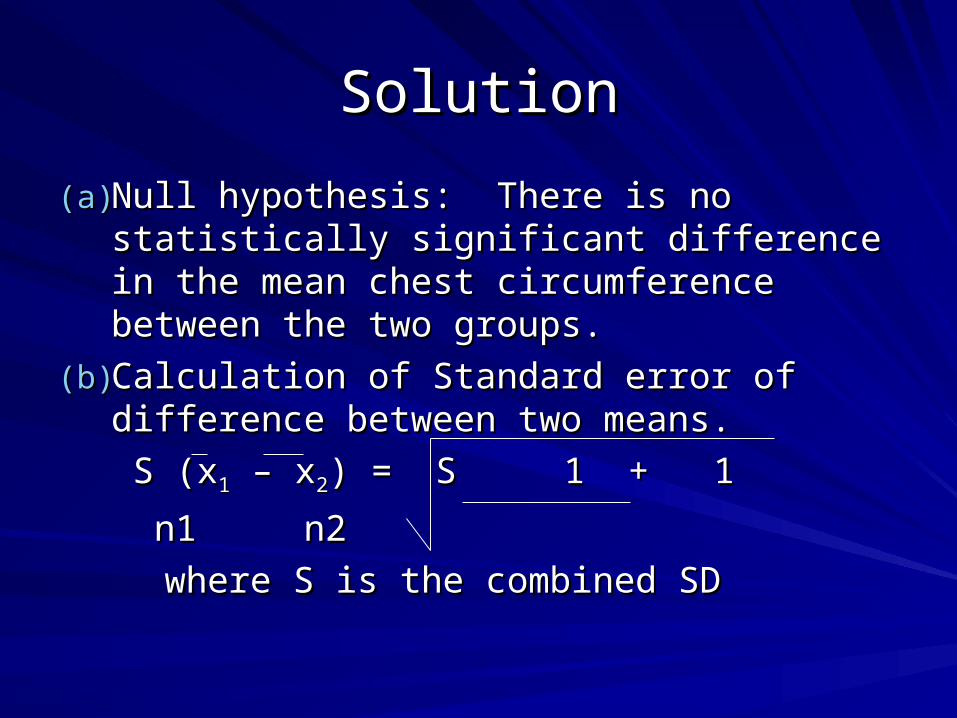
(a)(a) Null hypothesis: There is no statistically Null hypothesis: There is no statistically significant difference in the mean chest significant difference in the mean chest circumference between the two groups.circumference between the two groups.

(b)(b) Calculation of Standard error of Calculation of Standard error of difference between two means.difference between two means.

S (xS (x11 – x – x22) = S 1 + 1) = S 1 + 1

n1 n2n1 n2

where S is the combined SDwhere S is the combined SD

Solution contd.Solution contd.

Combined SD (S) =Combined SD (S) =

SS1122 (n (n11-1) + S-1) + S22

22 (n (n22-1)-1)

nn11 + n + n2 2 -2-2

where Swhere S11 and S and S22 are Standard deviations are Standard deviations

and nand n11 and n and n22 are the sample sizes of 1 are the sample sizes of 1stst

and 2and 2ndnd samples respectively. samples respectively.

Solution contd.Solution contd.In the given example, following are the In the given example, following are the values of mean, SD and sample sizevalues of mean, SD and sample size

MeanMean SDSD NN

First sampleFirst sample 48.548.5 4.53 4.53 1010

Second sampleSecond sample 34.834.8 4.574.57 1010

By substituting the values, we getBy substituting the values, we get

4.534.5322 (10-1) + 4.57 (10-1) + 4.5722 (10-1) (10-1)

10 + 10 - 210 + 10 - 2


Thus, we getThus, we get

S = 20.52 (9) + 20.88 (9)S = 20.52 (9) + 20.88 (9)

1818

= 184. 68 + 187.96= 184. 68 + 187.96

1818

= 372.65 /18 = 20.70 = 4.55 cm= 372.65 /18 = 20.70 = 4.55 cm


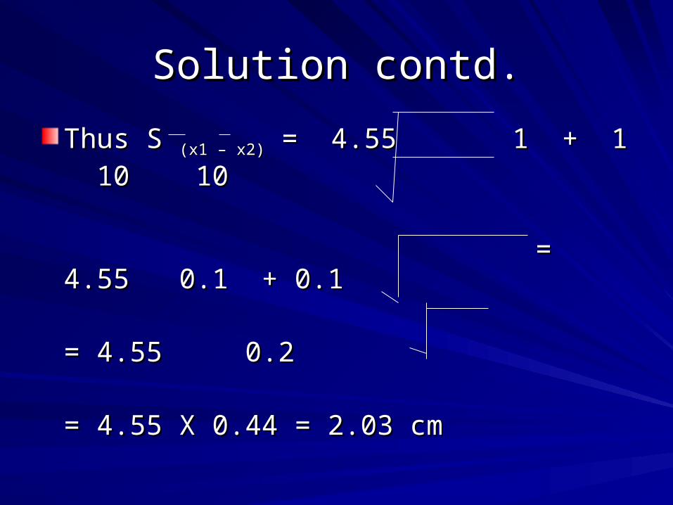
Thus S Thus S (x1 – x2)(x1 – x2) = 4.55 1 + 1 = 4.55 1 + 1

10 1010 10

= 4.55 0.1 + 0.1= 4.55 0.1 + 0.1

= 4.55 0.2= 4.55 0.2

= 4.55 X 0.44 = 2.03 = 4.55 X 0.44 = 2.03 cmcm


(c)(c) Calculation of t valueCalculation of t value

t = Xt = X11 – X – X22

S S (x1 – x2) (x1 – x2)

= 48.5 – 34.8= 48.5 – 34.8

2.032.03

= 13.7/2.03 = 6.75= 13.7/2.03 = 6.75


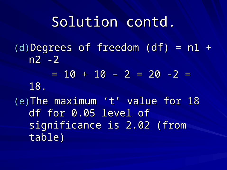
(d)(d) Degrees of freedom (df) = n1 + n2 -2Degrees of freedom (df) = n1 + n2 -2

= 10 + 10 – 2 = 20 -2 = 18.= 10 + 10 – 2 = 20 -2 = 18.

(e)(e) The maximum ‘t’ value for 18 df for 0.05 The maximum ‘t’ value for 18 df for 0.05 level of significance is 2.02 (from table)level of significance is 2.02 (from table)


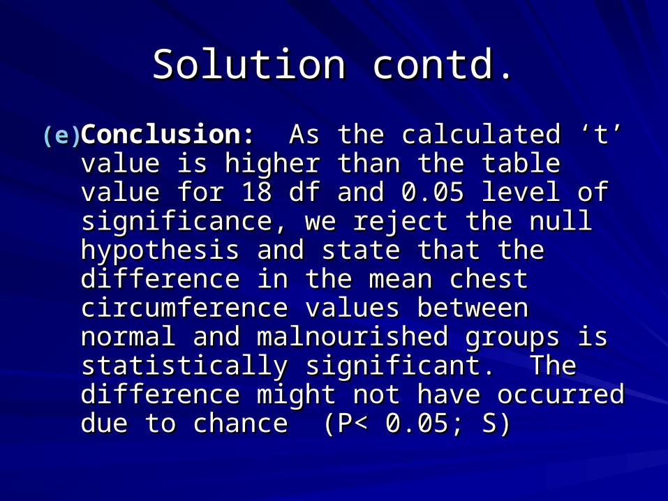
(e)(e) Conclusion:Conclusion: As the calculated ‘t’ value As the calculated ‘t’ value is higher than the table value for 18 df is higher than the table value for 18 df and 0.05 level of significance, we reject and 0.05 level of significance, we reject the null hypothesis and state that the the null hypothesis and state that the difference in the mean chest difference in the mean chest circumference values between normal circumference values between normal and malnourished groups is statistically and malnourished groups is statistically significant. The difference might not significant. The difference might not have occurred due to chance have occurred due to chance

(P< 0.05; S)(P< 0.05; S)

Paired ‘t’ testPaired ‘t’ test

This test is used where each person gives This test is used where each person gives two observations – before and after valuestwo observations – before and after values

For example, if the same person gives two For example, if the same person gives two observations before and after giving a new observations before and after giving a new drug – in such cases, this test is used.drug – in such cases, this test is used.

Example : 2Example : 2

In a clinical trial to evaluate a new In a clinical trial to evaluate a new tranquilizer drug in reducing anxiety tranquilizer drug in reducing anxiety scores of 10 patients, the following scores of 10 patients, the following data are recorded (next page). Find data are recorded (next page). Find out whether the drug is significantly out whether the drug is significantly effective in reducing anxiety score effective in reducing anxiety score (Table ‘t’ value at 9 df at 0.05 level of (Table ‘t’ value at 9 df at 0.05 level of significance is 2.21)significance is 2.21)

Anxiety scoresAnxiety scores

Before Before

treatmenttreatment

2222 1818 1717 1919 2222 1212 1414 1111 1919 77

After After

treatmenttreatment

1919 1111 1414 1717 2323 1111 1515 1919 1111 88

Solution.Solution.

(a)(a) Null hypothesis: There is no statistically Null hypothesis: There is no statistically significant difference in the anxiety significant difference in the anxiety scores before and after treatment with scores before and after treatment with new tranquilizer drug.new tranquilizer drug.

(b)(b) Calculation of mean difference in the Calculation of mean difference in the anxiety scoresanxiety scores

Before Before

treat.treat.

(X(X11))

AfterAfter

treat.treat.

(X(X22))

Differ.Differ.

(X(X11 –X –X22))

= x = x

xx (x - x) (x - x) (x – x)(x – x)22

2222 1919 + 3+ 3 1.31.3 + 1.7+ 1.7 2.892.89

1818 1111 +7+7 1.31.3 + 5.7 + 5.7 32.4932.49

1717 1414 +3+3 1.31.3 + 1.7+ 1.7 2.892.89

1919 1717 + 2+ 2 1.31.3 + 0.7+ 0.7 0.490.49

2222 2323 - 1- 1 1.31.3 - 2.3- 2.3 5.295.29

1212 1111 + 1+ 1 1.31.3 - 0.3- 0.3 0.090.09

1414 1515 - 1- 1 1.31.3 - 2.3- 2.3 5.295.29

1111 1919 -88 1.31.3 -9.3-9.3 86.4986.49

1919 1111 + 8+ 8 1.31.3 + 6.7+ 6.7 44.8944.89

77 88 -11 1.31.3 - 2.3- 2.3 5.295.29

161161 148148 + 13+ 13 +13+13 ------ 186.1186.1


(b)(b) Calculation of Mean and SDCalculation of Mean and SD

Mean = Mean = ΣΣ x = +13 / 10 = +1.3 x = +13 / 10 = +1.3

nn

SD = SD = ΣΣ (x – x)2 (x – x)2

n-1n-1

= 186.1 / 9 = 4.54= 186.1 / 9 = 4.54

Calculation of Standard error of Calculation of Standard error of meanmean

(c)SE = SD/ n(c)SE = SD/ n

= 4.54 / 10= 4.54 / 10

= 4.54 / 3.16 = 1.43= 4.54 / 3.16 = 1.43


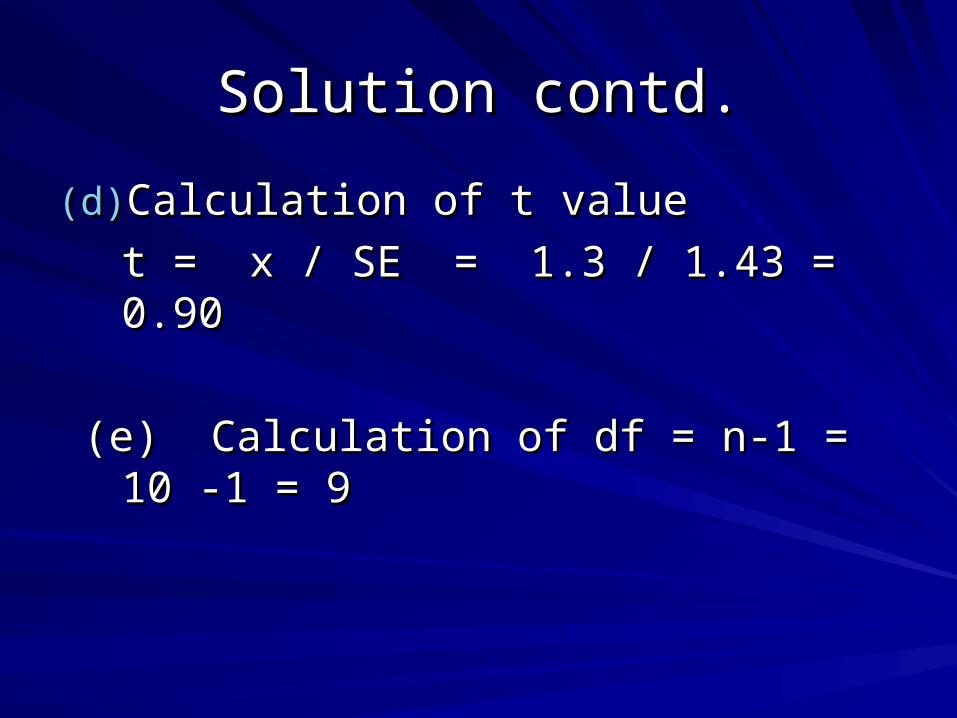
(d)(d) Calculation of t valueCalculation of t value

t = x / SE = 1.3 / 1.43 = 0.90t = x / SE = 1.3 / 1.43 = 0.90

(e) Calculation of df = n-1 = 10 -1 = 9(e) Calculation of df = n-1 = 10 -1 = 9


Conclusion:Conclusion: As the calculated ‘t’ value is As the calculated ‘t’ value is lower than the table value for df -9 at 5% lower than the table value for df -9 at 5% level (0.05 level) of significance, we accept level (0.05 level) of significance, we accept the null hypothesis and conclude that the null hypothesis and conclude that there is no statistically significant there is no statistically significant difference in the anxiety scores before and difference in the anxiety scores before and after treatment. The difference might have after treatment. The difference might have occurred because of chance (P>0.05; NS)occurred because of chance (P>0.05; NS)

Documents

Student t t est