Embed Size (px)
Citation preview

HAL Id: tel-01748148https://tel.archives-ouvertes.fr/tel-01748148v2
Submitted on 20 Jul 2007
HAL is a multi-disciplinary open accessarchive for the deposit and dissemination of sci-entific research documents, whether they are pub-lished or not. The documents may come fromteaching and research institutions in France orabroad, or from public or private research centers.
L’archive ouverte pluridisciplinaire HAL, estdestinée au dépôt et à la diffusion de documentsscientifiques de niveau recherche, publiés ou non,émanant des établissements d’enseignement et derecherche français ou étrangers, des laboratoirespublics ou privés.
Structures et modèles de calculs de réécritureGermain Faure
To cite this version:Germain Faure. Structures et modèles de calculs de réécriture. Génie logiciel [cs.SE]. Université HenriPoincaré - Nancy 1, 2007. Français. <NNT : 2007NAN10032>. <tel-01748148v2>

Departement de formation doctorale en informatique
Ecole doctorale IAEM Lorraine
Structures et modeles de calculs dereecriture
THESE
presentee et soutenue publiquement le 5 juillet 2007
pour l’obtention du
Doctorat de l’Universite Henri Poincare
(specialite informatique)
par
Germain Faure
Composition du jury
President : Dominique Mery Professeur, Universite Henri Poincare, Nancy, France
Rapporteurs : Gilles Dowek Professeur, Ecole Polytechnique, Palaiseau, FranceFemke van Raamdonk Professeur, Vrije Universiteit, Amsterdam, The Netherlands
Examinateurs : Horatiu Cirstea (directeur) Maıtre de Conferences, Universite Nancy II, Nancy, FranceClaude Kirchner (directeur) Directeur de recherche, INRIA, Nancy, France
Paul-Andre Mellies Charge de Recherches CNRS, Equipe PPS, Paris, France
Laboratoire Lorrain de Recherche en Informatique et ses Applications — UMR 7503

Mis en page avec LATEX

Ever tried. Ever failed. No matter. Try Again. Fail again. Fail better.
By Samuel Beckett in Worstward Ho
The road to wisdom ? Well, it’s plain and simple to express :Err and err and err again, but less and less and less.
By Piet Hein in Knuth’s Mathematical Writing
i

ii

Remerciements
Je suis heureux d’ecrire ces remerciements, profitant de l’occasion qui m’est donneed’exprimer ma gratitude.
Encadrement
Mon travail au sein de l’equipe Protheo a commence il y a deja plus de 5 ans. J’ai eteaccueilli par Claude Kirchner qui m’a fait decouvrir le monde de la recherche avec unenthousiasme certain. A chaque etape, sa vision d’ensemble a ete fort utile et la confiancequ’il m’a accordee a ete souvent precieuse. J’ai toujours ete chaleureusement accueillidans le bureau de Claude et j’en suis toujours sorti etonne de sa grande curiosite.
Pendant mon stage de licence et pendant ma these, j’ai lu a plusieurs reprises la thesed’Horatiu Cirstea, y decouvrant a chaque fois de nouvelles idees. Chaque jour d’avantage,j’apprecie la vivacite d’esprit et l’humour d’Horatiu. Mon seul regret est d’avoir trop parleet de ne pas m’etre laisse suffisamment interpeller. Sa presence au quotidien, melangede pedagogie, de simplicite et de patience, a ete extremement precieuse. Elle m’a permisde parfaire, par des remarques toujours pertinentes et constructives, mes competencesscientifiques mais aussi la qualite de ma redaction. Travailler avec lui a toujours ete unplaisir.
J’ai choisi d’aborder mon sujet de these en utilisant plusieurs approches dont une(semantique denotationnelle) est relativement eloignee de la culture de mes encadrantset de l’equipe. Cela fut certes complique, mais aussi tres instructif, m’obligeant toujoursa questionner ma demarche. Ce questionnement a ete parfois long et je tiens a remercierchacun de mes encadrants d’avoir permis ces differentes approches (ce qui necessite uneouverture d’esprit prononcee) et d’avoir respecte ces temps de questionnements.
Je tiens plus generalement a les remercier tres chaleureusement pour ce que chacunm’a apporte. Je suis conscient que je leur ai demande beaucoup et que l’investissementdont ils ont fait preuve est a la fois rare et de qualite.
Jury
C’est a la fois une joie et un honneur d’avoir un jury compose de scientifiques de toutpremier plan et issus de communautes relativement differentes. Je remercie chacun d’euxd’avoir accepte d’en faire partie (notamment Dominique Mery d’avoir accepte d’en etrele president) et de l’interet qu’ils ont porte a mon travail.
A plusieurs reprises, j’ai pu constater la pertinence et la pedagogie de Gilles Dowek etFemke van Raamsdonk. Leurs notes de cours (sur la theorie des types, respectivement lareecriture d’ordre superieur), leurs articles et leurs exposes m’ont appris beaucoup, aussi
iii
Remerciements
bien par leur contenu que par leur presentation. Les echanges avec Gilles ont toujours eteencourageants et plein de discernement et, la these de Femke a ete pour moi un modelede clarte et de rigueur.
Je les remercie tres fortement d’avoir accepte d’etre rapporteurs et d’avoir vu beaucoupplus que ce que j’avais ecrit. Je tiens a les remercier, ainsi que Paul-Andre Mellies, pourl’incroyable qualite de leurs questions qui constituent une mine d’or que je souhaiteexploiter au mieux.
Collaborations et cadre de travail
L’ensemble des membres de l’equipe Protheo a largement contribue a cette these,notamment par une lecture minutieuse d’une partie de mon manuscrit. Je tiens a lesremercier tres chaleureusement. Les membres permanents de l’equipe ainsi que Chan-tal Llorens m’ont offert un cadre de travail materiel tres satisfaisant. Je les remercienotamment d’avoir permis mes nombreux deplacements.
Mes journees de travail auront ete ponctuees par de nombreuses discussions, aussi bienavec des theoriciens fous (notamment Colin Riba) qu’avec des codeurs fous (notammentAntoine Reilles). J’apprecie toujours leur spontaneite et leur richesse.
Je tiens aussi a remercier les nombreux visiteurs de l’equipe Protheo pour m’avoirfait part de leurs remarques et interrogations. En particulier, Eduardo Bonelli m’a ins-pire l’approche decrite dans la premiere partie de cette these. Qu’il en soit sincerementremercie.
Apres avoir accepte d’encadrer mon stage de maıtrise au pied leve, Alexandre Miquelm’a a nouveau accueilli pour m’aider a approcher differemment mon sujet de these. Sesqualites scientifiques et pedagogiques ont contribue a ameliorer ma comprehension de lasemantique denotationnelle. Sa capacite tant a proposer une vision globale qu’a passerune journee entiere a comprendre pourquoi un diagramme commute m’impressionneencore aujourd’hui.
De nombreuses seances de travail avec Alexandre ont eu lieu au sein du laboratoirePPS. Je tiens a remercier l’ensemble des personnes qui ont rendu ces sejours agreableset instructifs. En particulier, je souhaite remercier tres vivement Delia Kesner pour nosechanges extremement stimulants.
Je remercie Emmanuel Hainry et Antoine Reilles de m’avoir incite a utiliser Vim etMutt qui sont devenus, grace a eux, mes outils preferes. Je les remercie aussi pour leuraide precieuse lors de la mise en page de ce document.
Enseignement
Durant ces quatre annees passees a Nancy, j’ai eu la chance de cotoyer des eleves et desenseignants qui m’ont donne envie de m’investir avec le plus de serieux et de devouementpossibles.
iv
Je tiens tout d’abord a remercier tres fortement mes eleves pour avoir accepte de mefaire confiance malgre des methodes de travail parfois originales, dans une periode ouj’etais encore hesitant sur mon approche de l’enseignement.
Que tous les enseignants avec qui j’ai travaille et qui, par l’exemple ou le contre-exemple, m’ont aide a tendre vers une pedagogie qui me ressemble soient remercies. Enparticulier, Brigitte Jaray s’est attachee a me transmettre une idee de l’enseignementfaite d’un savant melange de rigueur, de plaisir et de liberte. Qu’elle soit assuree de masincere gratitude.
Je souhaiterais remercier les enseignants qui m’ont donne, lorsque j’etais leur etu-diant, l’envie de faire ce metier. Merci a Odile Millet-Botta pour m’avoir fait decouvrirl’informatique fondamentale et pour m’avoir incite a postuler a l’ENS de Lyon. Mercia Jacques Mazoyer qui a su, a l’occasion de son cours de calculabilite, me transmettrepassion et intuitutions. Merci enfin a Jean-Pierre Jouannaud pour son excellent courssur la reecriture d’ordre superieur.
Pour finir. . .
Ce document etant a usage professionnel, je me suis limite aux remerciements direc-tement lies a ce contexte.
Neanmoins, je souhaite remercier toutes les personnes avec qui j’ai partage un bout dechemin une fois sorti du travail (les citer serait digne d’une enumeration a la Prevert).Je trouve rassurant de ne pas savoir ce que je dois reellement a chacun d’eux mais je lesremercie tres sincerement pour tout ce que nous avons partage et partageons. Merci enparticulier a ma famille pour son amour. Leur soutient affectif et materiel a toujours eteopportun.
Merci enfin a Daniel qui a toujours su m’apporter, en plus du reste, une ecoute attentiveet reconfortante dans mes nombreux moments d’hesitations.
v

Remerciements
vi

Table des matieres
Remerciements iii
Extended abstract 5
Introduction 11
I Filtrage d’ordre superieur dans le lambda-calcul 15
1 Normalisations dans le λ-calcul 17
1.1 Lambda-calcul simplement type et β-reduction . . . . . . . . . . . . . . . 18
1.2 Lambda-calcul pur et developpements . . . . . . . . . . . . . . . . . . . . 21
1.2.1 Lambda-calcul souligne . . . . . . . . . . . . . . . . . . . . . . . . 21
1.2.2 Developpements . . . . . . . . . . . . . . . . . . . . . . . . . . . . 22
1.2.3 Reduction parallele . . . . . . . . . . . . . . . . . . . . . . . . . . . 23
1.3 Lambda-calcul pur et super-developpements . . . . . . . . . . . . . . . . . 24
1.3.1 Creations de radicaux dans le λ-calcul . . . . . . . . . . . . . . . . 24
1.3.2 Lambda-calcul etiquete . . . . . . . . . . . . . . . . . . . . . . . . 26
1.3.3 Super-developpements . . . . . . . . . . . . . . . . . . . . . . . . . 27
1.3.4 Reduction parallele forte . . . . . . . . . . . . . . . . . . . . . . . . 29
2 Filtrage d’ordre superieur 31
2.1 Filtrage modulo β . . . . . . . . . . . . . . . . . . . . . . . . . . . . . . . 34
2.1.1 Definition . . . . . . . . . . . . . . . . . . . . . . . . . . . . . . . . 34
2.1.2 Filtrage d’ordre n . . . . . . . . . . . . . . . . . . . . . . . . . . . 34
2.1.3 Filtrage modulo βη . . . . . . . . . . . . . . . . . . . . . . . . . . 35
2.1.4 Filtrage de motifs a la Miller . . . . . . . . . . . . . . . . . . . . . 35
2.2 Filtrage modulo super-developpements . . . . . . . . . . . . . . . . . . . . 36
2.2.1 Definition . . . . . . . . . . . . . . . . . . . . . . . . . . . . . . . . 36
2.2.2 Comparaison avec le filtrage du second ordre . . . . . . . . . . . . 38
2.2.3 Comparaison avec le filtrage du troisieme ordre . . . . . . . . . . . 40
2.2.4 Comparaison avec le filtrage des motifs a la Miller . . . . . . . . . 41
2.2.5 Filtrage modulo super-developpements et η . . . . . . . . . . . . . 41
3 Algorithmes de filtrage d’ordre superieur 43
3.1 Filtrage modulo super-developpements . . . . . . . . . . . . . . . . . . . . 43
3.1.1 Regles . . . . . . . . . . . . . . . . . . . . . . . . . . . . . . . . . . 43
1
Table des matieres
3.1.2 Proprietes de l’algorithme . . . . . . . . . . . . . . . . . . . . . . . 47
3.2 Filtrage modulo η et super-developpements . . . . . . . . . . . . . . . . . 55
3.2.1 Regles . . . . . . . . . . . . . . . . . . . . . . . . . . . . . . . . . . 55
3.2.2 Minimalite pour les motifs a la Miller . . . . . . . . . . . . . . . . 57
3.3 Filtrage du second ordre . . . . . . . . . . . . . . . . . . . . . . . . . . . . 59
3.3.1 Algorithme de Huet et Lang . . . . . . . . . . . . . . . . . . . . . . 59
3.3.2 Filtrage modulo super-developpements et types . . . . . . . . . . . 61
3.3.3 Algorithme base sur les super-developpements . . . . . . . . . . . . 63
II Structures of the rewriting calculus 65
4 The rewriting calculus 67
4.1 Syntax . . . . . . . . . . . . . . . . . . . . . . . . . . . . . . . . . . . . . . 68
4.2 Operational semantics . . . . . . . . . . . . . . . . . . . . . . . . . . . . . 70
4.2.1 Matching . . . . . . . . . . . . . . . . . . . . . . . . . . . . . . . . 71
4.2.2 Evaluation rules . . . . . . . . . . . . . . . . . . . . . . . . . . . . 72
4.3 Confluence . . . . . . . . . . . . . . . . . . . . . . . . . . . . . . . . . . . 74
4.3.1 Syntactical restrictions . . . . . . . . . . . . . . . . . . . . . . . . . 74
4.3.2 Reduction strategies . . . . . . . . . . . . . . . . . . . . . . . . . . 75
4.3.3 Encoding Klop’s counter example in the ρ-calculus . . . . . . . . . 76
4.4 Expressiveness . . . . . . . . . . . . . . . . . . . . . . . . . . . . . . . . . 78
4.5 Extensions of the ρ-calculus . . . . . . . . . . . . . . . . . . . . . . . . . . 79
4.5.1 The ρstk-calculus . . . . . . . . . . . . . . . . . . . . . . . . . . . . 79
4.5.2 The ρd-calculus . . . . . . . . . . . . . . . . . . . . . . . . . . . . . 82
4.6 Higher-order matching in the ρ-calculus . . . . . . . . . . . . . . . . . . . 82
4.6.1 Matching in the λ-calculus vs matching in the ρ-calculus . . . . . . 82
4.6.2 Matching in the ρ-calculus needs unification . . . . . . . . . . . . . 84
4.6.3 Extensionality in the ρ-calculus . . . . . . . . . . . . . . . . . . . . 84
5 The explicit ρ-calculus 87
5.1 Explicit substitution ρs . . . . . . . . . . . . . . . . . . . . . . . . . . . . 88
5.1.1 Syntax of ρs . . . . . . . . . . . . . . . . . . . . . . . . . . . . . . 89
5.1.2 Operational semantics of ρs . . . . . . . . . . . . . . . . . . . . . . 90
5.2 Explicit matching ρm . . . . . . . . . . . . . . . . . . . . . . . . . . . . . . 92
5.2.1 Syntax of ρm . . . . . . . . . . . . . . . . . . . . . . . . . . . . . . 92
5.2.2 Operational semantics of ρm . . . . . . . . . . . . . . . . . . . . . . 92
5.3 Explicit substitution and explicit matching ρx
. . . . . . . . . . . . . . . . 95
5.3.1 Syntax of ρx
. . . . . . . . . . . . . . . . . . . . . . . . . . . . . . 95
5.3.2 Operational semantics of ρx
. . . . . . . . . . . . . . . . . . . . . . 97
5.4 Properties of ρx
. . . . . . . . . . . . . . . . . . . . . . . . . . . . . . . . . 99
5.4.1 Proof scheme . . . . . . . . . . . . . . . . . . . . . . . . . . . . . . 99
5.4.2 Soundness of explicit substitutions . . . . . . . . . . . . . . . . . . 102
5.4.3 Termination of the constraint handling rules . . . . . . . . . . . . . 103
2
Table des matieres
5.4.4 Confluence of the sub-relations . . . . . . . . . . . . . . . . . . . . 111
5.4.5 Parallel version of the ρδ . . . . . . . . . . . . . . . . . . . . . . . 114
5.4.6 Yokouchi-Hikita’s diagram modulo and confluence of ρx
. . . . . . 114
5.5 Implementation in the Tom language . . . . . . . . . . . . . . . . . . . . . 117
5.6 Explicit substitutions with generalized de Bruijn indices in the ρ-calculus 119
5.6.1 Explicit substitution with de Bruijn indices in the λ-calculus . . . 119
5.6.2 Explicit substitutions with generalized de Bruijn indices in theρ-calculus . . . . . . . . . . . . . . . . . . . . . . . . . . . . . . . . 120
6 Confluence of pattern-based λ-calculi 125
6.1 The dynamic pattern λ-calculus . . . . . . . . . . . . . . . . . . . . . . . . 126
6.1.1 Syntax . . . . . . . . . . . . . . . . . . . . . . . . . . . . . . . . . . 126
6.1.2 Operational semantics . . . . . . . . . . . . . . . . . . . . . . . . . 127
6.2 Confluence of the dynamic pattern λ-calculus . . . . . . . . . . . . . . . . 128
6.2.1 The parallel reduction . . . . . . . . . . . . . . . . . . . . . . . . . 129
6.2.2 Stability of Sol . . . . . . . . . . . . . . . . . . . . . . . . . . . . . 129
6.2.3 Confluence of the dynamic pattern λ-calculus . . . . . . . . . . . . 130
6.2.4 Confluence issues with linear patterns . . . . . . . . . . . . . . . . 135
6.3 Instantiations of the dynamic pattern λ-calculus . . . . . . . . . . . . . . 137
6.3.1 λ-calculus with Patterns . . . . . . . . . . . . . . . . . . . . . . . . 138
6.3.2 Rewriting calculi . . . . . . . . . . . . . . . . . . . . . . . . . . . . 139
6.3.3 Pure pattern calculus . . . . . . . . . . . . . . . . . . . . . . . . . 140
6.3.4 λ-calculus with constructors . . . . . . . . . . . . . . . . . . . . . . 142
III Categorical semantics of the parallel λ-calculus 145
7 Categorical semantics of the λ-calculus 147
7.1 Cartesian closed categories and reflexive objects . . . . . . . . . . . . . . . 147
7.2 Interpretation of pure λ-terms . . . . . . . . . . . . . . . . . . . . . . . . . 149
7.3 Examples in Scott domains . . . . . . . . . . . . . . . . . . . . . . . . . . 150
7.4 Completeness . . . . . . . . . . . . . . . . . . . . . . . . . . . . . . . . . . 152
8 Categorical semantics of the parallel λ-calculus 155
8.1 The parallel λ-calculus . . . . . . . . . . . . . . . . . . . . . . . . . . . . . 156
8.1.1 The core calculus . . . . . . . . . . . . . . . . . . . . . . . . . . . . 156
8.1.2 Extensions of the equational theory . . . . . . . . . . . . . . . . . 157
8.1.3 Linearity . . . . . . . . . . . . . . . . . . . . . . . . . . . . . . . . 157
8.2 Monads and algebras . . . . . . . . . . . . . . . . . . . . . . . . . . . . . . 158
8.3 Aggregation monads . . . . . . . . . . . . . . . . . . . . . . . . . . . . . . 161
8.3.1 Notion of aggregation . . . . . . . . . . . . . . . . . . . . . . . . . 161
8.3.2 Typical examples . . . . . . . . . . . . . . . . . . . . . . . . . . . . 163
8.3.3 Algebras and linear morphisms . . . . . . . . . . . . . . . . . . . . 164
8.3.4 Strong notion of aggregation . . . . . . . . . . . . . . . . . . . . . 167
3
Table des matieres
8.4 Model of the parallel λ-calculus . . . . . . . . . . . . . . . . . . . . . . . . 1688.4.1 Definition . . . . . . . . . . . . . . . . . . . . . . . . . . . . . . . . 1688.4.2 Interpreting parallel λ-terms . . . . . . . . . . . . . . . . . . . . . 169
8.5 Examples in Scott domains . . . . . . . . . . . . . . . . . . . . . . . . . . 171
9 Completeness by syntactical models 1759.1 The notion of T-per . . . . . . . . . . . . . . . . . . . . . . . . . . . . . . 1759.2 The ccc structure of T-PER . . . . . . . . . . . . . . . . . . . . . . . . . . 1789.3 The aggregation monad of T-PER . . . . . . . . . . . . . . . . . . . . . . 181
9.3.1 The boxing monad . . . . . . . . . . . . . . . . . . . . . . . . . . . 1819.3.2 The aggregation monad . . . . . . . . . . . . . . . . . . . . . . . . 184
9.4 Completeness . . . . . . . . . . . . . . . . . . . . . . . . . . . . . . . . . . 1869.4.1 Proof sketch . . . . . . . . . . . . . . . . . . . . . . . . . . . . . . 1879.4.2 Reflexivity . . . . . . . . . . . . . . . . . . . . . . . . . . . . . . . 1879.4.3 Algebraicity . . . . . . . . . . . . . . . . . . . . . . . . . . . . . . . 1889.4.4 Distributivity axiom . . . . . . . . . . . . . . . . . . . . . . . . . . 1889.4.5 Adapted model . . . . . . . . . . . . . . . . . . . . . . . . . . . . . 1899.4.6 Completeness result . . . . . . . . . . . . . . . . . . . . . . . . . . 191
10 Constructing a model of the parallel λ-calculus 19310.1 First method . . . . . . . . . . . . . . . . . . . . . . . . . . . . . . . . . . 193
10.1.1 Algebraicity . . . . . . . . . . . . . . . . . . . . . . . . . . . . . . . 19410.1.2 Reflexivity . . . . . . . . . . . . . . . . . . . . . . . . . . . . . . . 19410.1.3 Distributivity axiom . . . . . . . . . . . . . . . . . . . . . . . . . . 19510.1.4 Typical use . . . . . . . . . . . . . . . . . . . . . . . . . . . . . . . 195
10.2 Second method . . . . . . . . . . . . . . . . . . . . . . . . . . . . . . . . . 19610.2.1 Algebraicity . . . . . . . . . . . . . . . . . . . . . . . . . . . . . . . 19710.2.2 Reflexivity . . . . . . . . . . . . . . . . . . . . . . . . . . . . . . . 19710.2.3 Distributivity axiom . . . . . . . . . . . . . . . . . . . . . . . . . . 19910.2.4 Typical use . . . . . . . . . . . . . . . . . . . . . . . . . . . . . . . 200
IV Epilogue 203
Conclusion et travaux futurs 205
Bibliographie 209
4

Extended abstract
In the 1930s, A. Church introduced the λ-calculus as a theoretical framework for describ-ing functions and their evaluation and gave a negative answer to the Entscheidungsprob-lem [Chu36, Chu41]. Ever since, the λ-calculus greatly influenced functional program-ming languages and is even very often quoted as the paradigm of functional languages.Interestingly, in practice, functional languages strongly rely on pattern-matching. This isthe case of O’caml [LDG+04], Haskell [Pey03], Lisp [All78] or F# [Pic07]. A “speed-up”of the λ-calculus with patterns where variable abstraction is replaced by pattern abstrac-tion was then emerging from the practice of functional programming design [Pey87].
On one hand, following S. Peyton Jones the so-called λ-calculus with patterns wasintroduced [Oos90, KOV07]. Latter on, many different pattern-based λ-calculi arose inthe context of the functional programming. For example, we can quote the basic patternmatching calculus [Kah03] and the pure pattern calculus [JK06].
On the other hand, studying rewriting —where pattern-matching is a fundamentaloperation— and especially rewriting strategies led to the rewriting calculus [CK98b]. Therewriting calculus, a.k.a. the ρ-calculus, was introduced to make explicit all the ingre-dients of rewriting such as rules, rule applications, strategies and results [CK01, Cir00].The ρ-calculus is a generalization of the λ-calculus with pattern-matching features andterm collections. The work presented here was initially motivated by its study.
There are thus several pattern λ-calculi and each of them has many syntactical vari-ants depending on the intended use: define the relationship between pattern-calculiand first-order term rewriting [CHW06] or graph rewriting [BBCK06, Ber05], encodeobject λ-calculi [CKL01], study type systems [BCKL03, Wac05], add dynamic pat-terns [BCKL03, JK06], etc.. This plethora of calculi raises the following questions: whatare the basic ingredients on which all these calculi are based, how do these componentsinteract and what is the computational and expressive power of such calculi. To answerthese questions there are many possible approaches and we chose four of them in thisthesis that are summarized below. A more detailed presentation of each part is givenafterwards.
To play with the computational and expressive power of pattern-based λ-calculi, wecan study higher-order matching where λ-terms (purely functional programs) are re-placed by ρ-terms (functional programs with pattern-matching). The work already donein the typed λ-calculus is not transposable, as the simply typed ρ-calculi is not normal-izing [Wac05]. In fact, the normalizing simply typed ρ-calculus uses (weakly) dependenttypes built using Π-abstractions on patterns. Then for a given matching equation, togive the types of the matching variables almost corresponds to give the solutions. So,it is of strong interest to study higher-order matching in an untyped context. In thisthesis, we analyze higher-order matching in the untyped λ-calculus as a preliminary step
5

Extended abstract
to solve matching in the ρ-calculus.
Most of the presentations of the ρ-calculus use meta-level matching and substitutionapplication but the explicit definition of these operations underlines some interactionsbetween both operations. Following the works on explicit substitutions in the λ-calculus,we define and study a ρ-calculus with explicit matching and substitution application.We show that it is a useful theoretical back-end for implementations of pattern-basedλ-calculi and especially rewriting-calculi.
To compare the expressiveness and the confluence of pattern-based λ-calculi, we in-troduce and study a general confluent formalism where the way pattern-abstractions areapplied is axiomatized. This is done in the third part of this thesis.
Another way to understand the basic ingredients of pattern-based λ-calculi is to studya denotational semantics for the rewriting calculus. This raises many questions andchallenges that are not intrinsically related to the ρ-calculus but that already appearin the parallel λ-calculus. This is why we propose a clear categorical semantics for theparallel λ-calculus that can be seen as a first step towards a denotational semantics forthe ρ-calculus.
We now give a more detailed presentation for each of the corresponding contributions.
Higher-order matching modulo superdevelopments We often need to decide β-equivalence. This is the case for the transformation of strict functional programs (pro-grams as λ-terms) and for the proof theory (proofs as λ-terms). Since β-equivalence isundecidable, we usually restrict to typed λ-terms in order to recover decidability. Butwhen we transform functional programs with pattern-matching (programs as ρ-terms)and when we consider [Wac05] rich proof terms for the generalized deduction modulo(proofs as ρ-terms), β-equivalence has to be replaced by the equational theory of theρ-calculus.
The equivalence in the ρ-calculus is also undecidable (as it includes β-equivalence).But unlike in the λ-calculus, the restriction to typed ρ-terms is not suitable in the contextof higher-order matching. In fact, the normalizing simply typed ρ-calculus [Wac05] uses(weakly) dependent types built using Π-abstractions on patterns. Then for a givenmatching equation, to give the types of the matching variables almost corresponds togive the solutions.
Consequently, the work already done concerning higher-order matching in the simplytyped λ-calculus is not transposable. This is why we propose a different approach basedon a restriction of β-conversion [MS01]. The usual approximation of β-normal formsis given by complete finite developments with the corresponding parallel reduction ofTait and Martin-Lof. An extension of finite developments, called superdevelopments,was introduced in [Raa93] to prove the confluence of a general class of reduction systemscontaining the λ-calculus and term rewrite systems.
A superdevelopment is a reduction sequence that may reduce the redexes of the term,its residuals and some created redexes. The redexes created by the substitution of avariable in a functional position by a λ-abstraction are not reduced. The approximationgiven by superdevelopments of a second-order term coincides with its β-normal form. Su-
6
perdevelopments can be alternatively defined using a suitable parallel reduction [Acz78]that generalises the parallel reduction of Tait and Martin-Lof.
We consider here matching equations built over untyped λ-terms and solve them mod-ulo superdevelopments. The matching problems are of interest particularly because theset of matches modulo superdevelopments contains, but is not restricted to, second-orderβ-matches. Moreover, the restriction of the β-conversion needed in the case of pattern-matching a la Miller [Mil91] is subsumed by superdevelopments and thus matchingmodulo superdevelopments is complete w.r.t. the matching a la Miller.
We propose sound and complete algorithms for the matching in the pure λ-calculusmodulo superdevelopments and for the second-order matching modulo β. The algo-rithms are presented using transformation rules [MM82] based on the parallel reductionof Aczel while the intuitions and the proofs are based on the equivalent notion of su-perdevelopments. This leads to an intuitive presentation and to simpler proofs.
A ρ-calculus with explicit constraint applications Substitutions and pattern-matchingare fundamental operations of the rewriting calculus that are inherited respectively fromthe λ-calculus and from rewriting. To perform pattern-matching, evaluation rules of theρ-calculus use helper functions that are indeed implicit computations: all the computa-tions related to the considered matching theory belong to the meta-level. These compu-tations are conceptually and computationally important in all matching theories, fromsyntactic ones to quite elaborated ones like associative-commutative theories [Eke95]. Inconcrete implementations, substitutions and pattern-matching should be separated andshould interact with one another. In particular, we want matching related computationsand applications of substitutions to be explicit.
A first step toward an explicit handling of the matching related computations wasthe introduction of matching problems as part of the ρ-calculus syntax [CKL02]. Moreprecisely, the matching constraints represent constrained terms which are eventuallyinstantiated by the substitution obtained as solution of the corresponding matchingproblem (if such a solution exists).
We study two versions of the ρ-calculus, one with explicit matching and one with ex-plicit substitutions (following the works on λ-calculi with explicit substitutions [ACCL91,Les94, Ros96]), together with a version that combines the two and considers efficiencyissues and more precisely the composition of substitutions. This allows us to isolate thefeatures absolutely necessary in both cases and to analyze the issues related to the twoapproaches. The result is a full calculus that enjoys the usual good properties of explicitsubstitutions (conservativity, termination) and which is confluent. We show that theρ-calculus, and especially explicit ρ-calculi, are suitable as a theoretical back-end forimplementations of rewriting-based languages.
This work is implemented in the Tom language [BBK+06] as an interpreter for theρ-calculus.
Confluence of pattern-based λ-calculi Each of the pattern-based calculi mentionedbefore differs on the way patterns are defined and on the way pattern abstractions
7

Extended abstract
are applied. Thus, patterns can be simple variables like in the λ-calculus, algebraicterms like in the algebraic rewriting calculus [CLW03], special (static) patterns thatsatisfy certain (semantic or syntactic) conditions like in the λ-calculus with patterns ordynamic patterns that can be instantiated and possibly reduced like in the pure patterncalculus and some versions of the rewriting calculus. The underlying matching theorystrongly depends on the form of the patterns and can be syntactic, equational or moresophisticated [JK06, BCKL03].
Although some of these calculi just extend the λ-calculus by allowing pattern abstrac-tions instead of variable abstractions, the confluence of these formalisms is lost when norestrictions are imposed.
Several approaches are then used to recover confluence. One of these techniques con-sists in syntacticly restricting the set of patterns and then showing that the reductionrelation is confluent for the chosen subset. This is done for example in the λ-calculuswith patterns and in the ρ-calculus (with algebraic patterns). The second techniqueconsiders a restriction of the initial reduction relation (that is, a strategy) to guaranteethat the calculus is confluent on the whole set of terms. This is done for example in thepure pattern calculus where the matching algorithm is a partial function whereas anyterm is a pattern.
Nevertheless, we can notice that in practice the proof methods share the same structureand that each variation on the way pattern abstractions are applied needs another proofof confluence. There is thus a need for a more abstract and more modular approach. Apossible way to have a unified approach for proving the confluence is the application of thegeneral and powerful results on the confluence of higher-order rewrite systems [KOR93,MN98, Ter03]. Although these results have already been applied for some particularpattern-calculi [BK07] the encoding seems to be rather complex for some calculi and inparticular for a general setting that encompasses several calculi. Moreover, it would beinteresting to have a framework where the expressiveness and (confluence) properties ofthe different pattern calculi can be compared.
We thus show [CF07] that all the pattern-based calculi can be expressed as a generalcalculus parameterized by a function that defines the underlying matching algorithmand thus the way pattern abstractions are applied. This function can be instantiated(implemented) by a unitary matching algorithm as in [CK01, JK06] but also by ananti-pattern matching algorithm [KKM07] or it can be even more general [LHL07]. Wepropose a generic confluence proof where the way pattern abstractions are applied isaxiomatized. Intuitively, the sufficient conditions to ensure confluence guarantee thatthe (matching) function is stable by substitution and by reduction.
We apply our approach to several classical pattern calculi, namely the λ-calculus withpatterns, the pure pattern calculus, the rewriting calculus and the λ-calculus with con-structors [AMR06]. For all these calculi, we give the encodings in the general frameworkfrom which we derive the proofs of confluence. This approach does not provide conflu-ence proofs for free but it establishes a proof methodology and isolates the key pointsthat make the calculi confluent. It can also point out some matching algorithms that al-though natural at the first sight can lead to non confluent reduction in the correspondingcalculus.
8

A categorical semantics of the parallel λ-calculus The starting point of this workwas the semantical study of the ρ-calculus. A Scott semantics revealed the similarity(up to the fact that term collections are not systematically required to be associative,commutative and/or idempotent) between term collections of the ρ-calculus interpretedas the binary join and Boudol’s parallel construct of the parallel λ-calculus [Bou94] .
Formally, the parallel λ-calculus is obtained by extending the pure λ-calculus with abinary operator that intuitively represents the parallel execution. The parallel λ-calculusadds to the equational theory of the pure λ-calculus the single equational axiom (δ)
expressing the distributivity of function application w.r.t. parallel aggregation. Theparallel λ-calculus was initially introduced as a tool to study full-abstraction of theinterpretation of λ-terms in Scott domains. In this framework, Boudol extended theinterpretation of pure λ-terms to the parallel construction using the join operation.
Scott semantics is well-suited to achieve full-abstraction but it is not sufficient to cap-ture neither the basic equational theory of the calculus nor many interesting extensionsof it—typically when dealing with extensionality. In the same way, interpreting the par-allel operator as the binary join automatically validates associativity, commutativity andidempotence, although on a purely syntactical level, these equational axioms are clearlyindependent from the basic equational axiom (β) and (δ). For these reasons, there is aneed for a more general and more modular semantics.
We define [FM07] a sound and complete categorical semantics for the parallel λ-calculus, based on a notion of aggregation monad which is modular w.r.t. associativity,commutativity and idempotence. This semantics is complete in a very strong sense: foreach extension T of the basic equational theory of the parallel λ-calculus, it is possibleto find a reflexive object such that the equational theory induced by the interpretationof parallel λ-terms in this object is exactly the theory T.
To prove completeness, we introduce a category of partial equivalence relations adaptedto parallelism, in which any extension of the basic equational theory of the calculus isinduced by some model. We also present abstract methods to construct models of theparallel λ-calculus in categories where particular equations have solutions, such as thecategory of Scott domains and its variants, and check that G. Boudol’s original semanticsis a particular case of ours.
The semantical study of the ρ-calculus also pointed out many interesting problemsrelated to the interaction between a mechanism of pattern-matching and the parallelconstruct. These problems helped us to grasp the importance of linear terms which playa central role in the proof of completeness (Boudol’s shift towards the λ-calculus withresources [BCL99] seems to be motivated by similar reasons).
We think that the categorical semantics introduced here will contribute to a betterunderstanding of the interaction between pattern-matching and the parallel construct,and thus will constitute a significant step towards a denotational semantics for the ρ-calculus.
9

Extended abstract
10

Introduction
Plusieurs developpements recents montrent que les assistants a la preuve sont suffi-samment murs pour etre utilises soit pour formaliser des theories mathematiques nontriviales [Gon05, ADGR07, GWZ02, Fly07], soit pour specifier et etudier des programmesde grande taille [MPU07, Fil03, Ler06, BDL06].
Pourtant, la distance entre une preuve papier et une preuve realisee grace a un assistanta la preuve est toujours importante. Cette distance est en partie due a la necessite, dansle cas d’une preuve formelle, d’expliciter tous les raisonnements consideres y comprisles plus triviaux et c’est bien pour cela que les mathematiciens ne presentent pas leurspreuves dans des systemes formels.
There are good reasons why Mathematicians do not usually present theirproofs in fully formal style. It is because proofs are not only a means tocertainty, but also a means to understanding. Behind each substantial formalproof there lies an idea, or perhaps several ideas. The idea, initially perhapstenuous, explains why the result holds. The idea becomes Mathematics onlywhen it can be formally expressed, but that expression must be so couched asto reveal the idea; it will not do to bury the idea under the formalism.(Saunders MacLane)
Proofs really aren’t there to convince you something is true – they’re thereto show you why it is true.(Andrew Gleason)
De plus, l’utilisation des assistants a la preuve revele qu’un passage a l’echelle n’estpossible que si le formalisme sous-jacent possede une capacite calculatoire suffisante. Lareecriture est souvent choisie pour cette capacite a exprimer et implementer simplementle calcul. Par exemple, plusieurs extensions du calcul des constructions, formalisme a labase du projet Coq, combinent le λ-calcul et la reecriture [TG89, Bar91, JO95, Fer93,Bla05].
Les notions de regles et de relations de reecriture jouent donc un role fondamentaldans ce contexte, comme dans celui de la transformation de programmes [Vis05], de lasecurite des protocoles [Rus06], des politiques de controles d’acces [HJM06] , etc. Cesnotions sont aussi particulierement pertinentes pour manipuler des structures de donneesverifiant des invariants [Rei06, HJM06], c’est-a-dire pour maintenir la representationinterne de donnees en forme canonique par rapport a un systeme de reecriture.
Toutes ces applications de la reecriture utilisent explicitement ou implicitement lanotion de strategies [BKK96, Vis01b, KK04, Kir05, MOMV06] qui s’est imposee uni-versellement dans les langages a base de regles (Tom, Elan, Maude), certains langages
11

Introduction
en ayant meme fait un veritable paradigme de programmation (Stratego). Il est parti-culierement interessant de remarquer que l’ingredient fondamental de la reecriture, lefiltrage, est present dans la plupart de langages fonctionnels et intervient donc dans desapplications couvrant des domaines varies, comme par exemple le web [Bal06, Fri06] oula programmation parallele [CMV+06].
Pourtant, et de maniere tout a fait surprenante, le λ-calcul, modele de calcul particu-lierement bien etudie, repose sur une notion triviale de filtrage. Par exemple, S. Peyton-Jones insista sur l’importance d’etudier une generalisation du λ-calcul avec du filtrage,afin de proposer pour les langages fonctionnels un paradigme incluant de maniere pri-mitive le filtrage [Pey87].
Cette absence de filtrage dans le λ-calcul necessite de nombreux encodages tant il estvrai qu’il n’est pas adapte pour decrire de maniere simple des mecanismes de calcul.Cette problematique se retrouve par exemple dans le calcul des constructions qui a ete aplusieurs reprises enrichi de primitives de calcul [CP88, Bar91], dans la transformationde programmes [MS01, Sit01] ou l’on utilise de maniere intensive la primitive fold pourcontourner l’absence de filtrage, ou encore lorsque l’on souhaite donner une semantiqueaux langages a base de regles.
C’est pour toutes ces raisons que l’on voit emerger a partir des annees 90, de nom-breux calculs avec motifs introduits soit pour donner une semantique aux langages abase de regles comme le calcul de reecriture [CK01, Cir00, CK98a], soit dans le cadre dela programmation fonctionnelle comme le λ-calcul avec motifs [Oos90], le calcul basiquede filtrage [Kah03], le calcul pur de motifs [Jay04, JK06] et le λ-calcul avec construc-teurs [AMR06].
Introduit par H. Cirstea et C. Kirchner pour expliciter les mecanismes de la reecritureet des strategies, le calcul de reecriture ou ρ-calcul est in fine une generalisation du λ-calcul avec filtrage et agregation de termes. L’abstraction sur les variables est etendue enune abstraction sur les motifs et dans sa definition la plus generale, le calcul de reecriturepermet l’utilisation du filtrage modulo une theorie equationnelle a priori arbitraire,utilisant l’agregation pour collecter les differents resultats possibles. L’agregation determes, souvent appelee structure, peut donc etre assimilee a des collections.
Dans cette these, nous proposons differentes approches pour expliciter les ingredientsde base des calculs avec motifs en general et du ρ-calcul en particulier. Nous cherchonsa analyser le filtrage et l’agregation en presence de mecanismes d’ordre superieur et apreciser leurs interactions.
Dans une premiere partie, nous etudions le filtrage d’ordre superieur dans le λ-calcul.L’approche classique [Hue76, HL78] consistant a se restreindre au sous-ensemble destermes types est ici remplacee par une approche considerant les equations modulo unerestriction de la β-conversion. Cette restriction est suffisamment expressive pour traiterles equations du second-ordre et les equations sur les motifs d’ordre superieur a la Miller.En plus de ne pas dependre d’un systeme de types particulier, les algorithmes que nous
12

etudions n’introduisent pas de nouvelles variables de filtrage durant le processus deresolution.
Dans une deuxieme partie, nous proposons tout d’abord une extension du ρ-calcul oules operations fondamentales de filtrage et de l’application de substitutions sont renduesexplicites, generalisant ainsi les λ-calculs avec substitutions explicites. Nous etudionsensuite la propriete de coherence (confluence) des calculs avec motifs et nous montronsque cette etude peut etre realisee de maniere axiomatique sur les proprietes des algo-rithmes de filtrage utilises dans ces calculs. Nous isolons ainsi les proprietes implicitementutilisees dans les differentes preuves de confluence des λ-calculs avec motifs.
Dans la troisieme partie de cette these, nous introduisons une semantique categoriquedu λ-calcul parallele dont les premiers modeles donnes par G. Boudol en sont des casparticuliers. Nous montrons que cette semantique est correcte et complete. Nous donnonsplusieurs constructions possibles de tels modeles et notament dans les domaines de Scott.Ce travail montre que les notion d’operateur pour le parallelisme, de collection de termeset d’operateur de structure du ρ-calcul peuvent etre etudiees simultanement grace a lanotion plus generale de monades d’agregation.
Guide de lecture Ce document est divise en trois parties relativement independantes.Nous avons pour cela occasionnellement repete certaines definitions. L’interet est bien-sur de permettre une lecture non-lineaire du manuscrit.
Les chapitres 1, 4 et 7 de cette these sont introductifs et presentent respectivement lanormalisation dans le λ-calcul, le ρ-calcul et les modeles categoriques du λ-calcul.
Le chapitre 2 definit dans plusieurs contextes (types ou non) le filtrage d’ordre su-perieur dans le λ-calcul et donne plusieurs instances (filtrage modulo β, modulo super-developpements, second-ordre, motifs a la Miller etc.). Nous comparons ensuite leurexpressivite.
Dans le chapitre 3, nous developpons plusieurs algorithmes pour le filtrage d’ordresuperieur et plus specialement pour le filtrage modulo super-developpements dont lesproprietes (terminaison, correction et completude) sont precisement etudiees.
Le chapitre 5 introduit plusieurs extensions du ρ-calcul qui rendent explicite le filtragepuis l’application de substitutions. Nous etudions les proprietes de ces differents calculs(confluence) et montrons differentes interactions possibles entre le filtrage et les substi-tutions. Nous presentons une implementation de ces calculs, implementation simple maisefficace qui offre un interpreteur pour le calcul de reecriture.
Le chapitre 6 presente un calcul ou les motifs sont dynamiques, c’est-a-dire qu’ilspeuvent etre instancies et reduits. Nous proposons une preuve de confluence generiqueou la maniere dont le filtrage est realise est axiomatisee. Nous montrons que cette ap-proche s’applique a differents calculs avec motifs. Nous caracterisons aussi une classed’algorithmes de filtrage qui conduisent a des calculs non confluents.
Le chapitre 8 est consacre a la definition d’une semantique categorique pour le λ-calcul parallele. Nous introduisons les notions fondamentales de monades d’agregation
13

Introduction
et de termes lineaires. Nous illustrons enfin notre definition sur plusieurs exemples prisdans les domaines de Scott. Nous retrouvons notamment les premiers modeles du λ-calculparallele introduits par G. Boudol.
Dans le chapitre 9, nous prouvons la completude de la semantique du λ-calcul paral-lele introduite dans le chapitre 8. Nous introduisons pour cela une notion de modelessyntaxiques bases sur les « pers ».
Nous concluons notre etude des modeles du λ-calcul parallele en donnant dans lechapitre 10 deux methodes de constructions de tels modeles a partir de modeles verifiantcertaines equations. Nous illustrons ces constructions dans la categorie des domaines deScott ou ces equations ont des solutions interessantes.
Pour finir nous presentons plusieurs pistes pour prolonger le travail presente tout aulong de ce manuscrit.
Quelques notations ne sont pas uniformes d’une partie a une autre. Nous avons essaye achaque fois d’utiliser celles qui nous paraissaient les plus claires et les plus courammentutilisees suivant le contexte. Le choix final a ete fait en ayant en tete le conseil deWitehead :
A good notation sets the mind free to think about really important things.(Alfred North Witehead)
14

Premiere partie
Filtrage d’ordre superieur dans lelambda-calcul
15

Chapitre 1
Normalisations dans le λ-calcul
Contexte Dans ce chapitre, nous examinons la normalisation du λ-calcul munie de laβ-reduction dans un cadre type puis non type. Chacune des deux approches conduit,dans le chapitre suivant, a une etude differente du filtrage d’ordre superieur.
Nous proposons tout d’abord de ne considerer que des termes bien types. Restreinta ce sous-ensemble de termes, la β-reduction termine. Ensuite, au lieu de restreindrel’ensemble des termes, nous restreignons la β-reduction : nous considerons une premiererestriction donnee par les developpements et une seconde par les super-developpements.
Un developpement est une suite de reductions qui ne reduit que les residus des radicauxpresents dans le terme initial. Le theoreme des developpements finis (qui assure que detelles reductions sont toujours finies) apparaıt pour la premiere fois dans la preuve deconfluence du λI-calcul donnee par A. Church et J.R. Rosser [CR36]. La preuve generalepour le λ-calcul telle qu’elle est donnee dans [Hin78] illustre l’importance du theoremedes developpements finis dans toutes les preuves de confluence des λ-calculs.
La notion de super-developpements, introduite initialement pour prouver la confluenced’une classe generale de systemes de reductions contenant le λ-calcul et les systemes dereecriture [Raa93], generalise la notion de developpement en autorisant la reduction ad-ditionnelle de tous les radicaux crees et qui ne sont pas obtenus par la substitution d’unevariable en position fonctionnelle par une λ-abstraction. Le theoreme des developpementsfinis se generalise au theoreme des super-developpements finis.
Contributions Ce chapitre est introductif. Le lecteur peut consulter [Bar84, Bar92,Kri90, Raa96] pour plus de details et notamment pour les preuves des resultats cites. Lastructure de ce chapitre est en partie inspiree du chapitre 2 de [Raa96].
Plan du chapitre Le chapitre est organise est trois parties qui sont chacune une manieredifferente d’obtenir la normalisation dans le λ-calcul. Tout d’abord nous etudions dansla section 1.1, le λ-calcul simplement type pour lequel la β-reduction termine toujours.Les deux sections suivantes se place dans le cadre du λ-calcul non type, aussi appeleλ-calcul pur. Dans ce contexte, pour obtenir une reduction terminante nous conside-rons deux sous-ensembles de la β-reduction. Dans la section 1.2 nous considerons lesdeveloppements et dans la section 1.3 les super-developpements.
17

Chapitre 1 Normalisations dans le λ-calcul
1.1 Lambda-calcul simplement type et β-reduction
Nous rappelons ici les definitions de base du λ-calcul simplement type afin de fixer lesnotations. Cette section est donc une succession de definitions de base qui se terminentpar le theoreme de confluence et de forte normalisation du λ-calcul simplement type.
Definition 1.1 (Types) Etant donne un ensemble de types de base T0, l’ensemble T
des types est defini inductivement comme le plus petit ensemble
– contenant T0 ;– et tel que pour tous α,β ∈ T on a (α→ β) ∈ T.
Definition 1.2 (Ordre d’un type) L’ordre d’un type α denote o(α) est defini par :
– o(α) = 1 si α ∈ T0 ;– o(α→ β) = max(o(α) + 1, o(β)).
Definition 1.3 (Termes bien types) Soit K un ensemble de constantes ayant cha-cune un type unique. Pour chaque type α ∈ T, on suppose donne un ensemble de va-riables de ce type, denote Xα. L’ensemble X est defini comme l’union des ensembles Xα
supposes distincts, soit X = ∪α∈TXα.
Par definition, l’ensemble des termes bien types note Tt est
– le plus petit ensemble contenant toutes les constantes et toutes les variables ;– et clos par les regles suivantes :
– Si A est un element de Tt de type α → β et B est un element de Tt de type α,alors (AB) est un element de Tt de type β ;
– Si A est un element de Tt de type β et x est une variable de Xα, alors λx.A estun element de Tt de type α→ β.
On utilisera les lettres A,B,C pour designer des elements de Tt, les lettres a, b, c, f, g, hpour designer des constantes et les lettres x, y, z pour designer des variables.
Les atomes qui representent soit une variable soit une constante seront denotes par lalettre ε.
Pour une meilleure lisibilite, le terme (. . . ((ε A1) A2) . . .) An) sera souvent noteε(A1, A2, . . . , An), ou ε est un atome et ou A1, . . . , An sont des termes quelconques.
Etant donne un terme A1A2 par definition le terme dit en position applicative est pardefinition le terme A2 et le terme en position fonctionnelle est par definition le termeA1.
Definition 1.4 (Variables libres et liees) L’ensemble des variables libres d’un termeA note fv(A) et l’ensemble des variables liees note bv(A) sont definis par
fv(x) = x bv(x) = ∅fv(a) = ∅ bv(a) = ∅
fv(AB) = fv(A) ∪ fv(B) bv(AB) = bv(A) ∪ bv(B)
fv(λx.A) = fv(A)\x bv(λx.A) = bv(A) ∪ x
18
1.1 Lambda-calcul simplement type et β-reduction
Une variable x est dite libre dans A si x ∈ fv(A). Une variable qui n’est pas libre estdite liee. Un λ-terme qui ne contient pas de variables libres est dit clos.
Nous considerons les termes modulo α-conversion c’est-a-dire modulo renommage desvariables liees. De plus nous supposons la condition d’hygiene de Barendregt : les va-riables libres et liees ont des noms differents.
Definition 1.5 (Positions dans les λ-termes) L’ensemble des positions dans les λ-termes est l’ensemble 0, 1∗, c’est-a-dire l’ensemble des mots construits sur l’alphabet0, 1. L’operateur de concatenation sur les mots (et donc sur les positions) est denotepar la juxtaposition. Le mot vide est denote ǫ. On utilise la lettre q (eventuellementindexee) pour designer une position d’un λ-terme.
Nous utilisons le symbole q pour les positions ; la lettre p sera utilisee dans la suite pourles etiquettes. Nous utiliserons sans ambiguıte le symbole ǫ pour denoter le mot vide etle symbole ε pour denoter un atome.
Definition 1.6 (Ordre sur les positions) L’ordre sur les positions dans les λ-termesnote est defini par q1 q2 s’il existe une position q ′ telle que q1q
′ = q2.
Definition 1.7 (Positions d’un λ-terme) L’ensemble Pos(A) des positions d’un λ-terme A est defini par induction sur l’ensemble des termes :
– Pos(x) = ǫ
– Pos(c) = ǫ
– Pos(λx.A0) = ǫ ∪ 0q0|q0 ∈ Pos(A0)
– Pos(A0A1) = ǫ ∪ 0q0|q0 ∈ Pos(A0) ∪ 1q1|q1 ∈ Pos(A1)
La position ǫ est souvent appelee la position de tete.
Definition 1.8 (Sous-terme) Soit A un λ-terme et soit q un element de Pos(A). Lesous-terme de A a la position q, denotee Aq est defini par :
– A|ǫ = A
– (λx.A0)|0q0= A0|q0
– (A0A1)|0q0= A0|q0
– (A0A1)|1q1= A1|q1
Definition 1.9 (Substitutions) Soient A et B deux termes bien types. La substitutionde x par A dans B est denotee B[x := A] et definie par
– x[x := A] = A
– y[x := A] = y si y 6= x
– a[x := A] = a
– (λy.B0)[x := A] = λy.(B0[x := A])
– (B0B1)[x := A] = (B0[x := A])(B1[x := A])
Dans la definition precedente, le cas d’une λ-abstraction est correct puisque nousconsiderons les termes modulo α-conversion : un representant adequat est choisi poureviter d’eventuelles captures de variables.
19

Chapitre 1 Normalisations dans le λ-calcul
Definition 1.10 (Relation compatible) Une relation →R sur l’ensemble des termesest compatible si :
A→R B impliqueAC →R BC
CA →R CB
λx.A →R λx.B
pour tout C
Definition 1.11 (Notion de reduction) Une notion de reduction est une relation bi-naire sur l’ensemble des termes.
Definition 1.12 (Relation de reduction) Une relation de reduction est la fermeturecompatible de d’une notion de reduction.
Definition 1.13 (Notion de β-reduction) La notion de β-reduction est definie par
(λx.A)B → A[x := B]
et nous notons →β la relation de reduction associee.
La fermeture reflexive et transitive de →β est notee →→β. La fermeture reflexive, syme-trique est notee =β.
Dans ce manuscrit, nous confondrons sans ambiguıte la notion de reduction et larelation de reduction associee.
Definition 1.14 (Radical – Ordre d’un radical) Un radical est un terme qui peuts’ecrire sous la forme (λx.A)B. L’ordre d’un tel radical est l’ordre du type du terme λx.A.
Theoreme 1.15 (Normalisation forte de β [HS86]) La relation de β-reduction ter-mine sur l’ensemble des termes bien types.
Ce resultat a ete prouve pour la premiere fois par Turing (voir [Gan80]). Pour prouverce theoreme, plusieurs approches sont possibles. Par exemple, nous pouvons citer lamethode habituellement appelee methode des candidats de reductibilite et basee sur lesnotions introduites par Tait [Tai67].
Theoreme 1.16 (Confluence de β [Bar84]) La β-reduction est confluente sur l’en-semble des termes bien types.
Il existe de nombreuses preuves differentes de ce theoreme, voir par exemple [Bar84]et [HS86]. Le theoreme 1.15 nous assure de l’existence d’une β-forme normale, le theo-reme 1.16 nous assure de son unicite. On parle ainsi de termes β-normaux et de la formeβ-normale d’un terme.
20

1.2 Lambda-calcul pur et developpements
1.2 Lambda-calcul pur et developpements
Nous definissons les developpements comme un sous-ensemble de la β-reduction quine reduit que les radicaux presents dans le terme initial et leurs residus. Cette notion estformalisee par l’intermediaire du λ-calcul souligne : on souligne les β-radicaux presentsinitialement dans un terme et la β-reduction est remplacee par la β-reduction qui nereduit que les radicaux soulignes. Ainsi, les radicaux crees au fur et a mesure ne sontpas reduits (puisqu’ils ne sont pas soulignes).
1.2.1 Lambda-calcul souligne
Nous definissons l’ensemble des termes soulignes. Nous surchargeons sans ambiguıteles notations du λ-calcul simplement type pour le λ-calcul pur. Toutes les definitionsprecedentes n’utilisant pas les informations de type seront utilisees dans le λ-calcul pursans etre repetees ici.
Definition 1.17 (Termes soulignes) Soient X un ensemble denombrable et infini devariables et K un ensemble de constantes. L’ensemble des termes soulignes Ts est
– le plus petit ensemble contenant toutes les constantes et toutes les variables ;– et clos par les regles suivantes :
– Si A et B sont des elements de l’ensemble Ts alors (AB) est un element de Ts ;– Si A est un element de Ts et x est une variable de X , alors λx.A est un element
de Ts ;– Si A et B sont des elements de l’ensemble Ts alors (λx.A)B appartient a Ts.
L’ensemble des termes soulignes n’est pas clos par sous-terme : par exemple le termeλx.A n’en est pas un element.
Definition 1.18 (Relation de β-reduction) La relation de β-reduction est definiesur l’ensemble des termes soulignes Ts par
(λx.A)B →β A[x := B]
La β-reduction consomme a chaque etape de reduction un radical souligne, peut endupliquer mais ne peut pas en creer. C’est ainsi une relation qui termine (theoreme 1.21).
Exemple 1.19 (Terminaison) Il n’existe pas de reduction infinie a partir du terme(λx.xx)(λx.xx). Son β-reduit (λx.xx)(λx.xx) est bien en forme β-normale puisqu’il necontient pas de radical souligne.
Exemple 1.20 (Duplication et reduction d’un radical) Un radical souligne peutetre duplique et ensuite chaque duplicata peut etre β-reduit.
(λx.xx)((λy.y)z) →β ((λy.y)z))((λy.y)z))
→β z((λy.y)z))
→β zz
21

Chapitre 1 Normalisations dans le λ-calcul
Theoreme 1.21 (Normalisation forte de β [Bar84]) La relation de β-reduction estterminante sur l’ensemble des termes soulignes.
Theoreme 1.22 (Confluence de β [Bar84]) La β-reduction est confluente sur l’en-semble des termes soulignes.
1.2.2 Developpements
Les termes du λ-calcul pur sont definis de la meme maniere que dans le λ-calculsimplement type mais en enlevant toutes les contraintes sur les types. Nous donnonsneanmoins leur definition.
Definition 1.23 (Termes) Soient K un ensemble de constantes et X un ensemble devariables. L’ensemble des termes du λ-calcul, note T est
– le plus petit ensemble contenant toutes les constantes et toutes les variables ;– et clos par les regles suivantes :
– Si A et B sont des elements de l’ensemble T alors (AB) est un element de T ;– Si A est un element de T et x est une variable de X , alors λx.A est un element
de T .
Nous pouvons remarquer qu’il existe une injection canonique de l’ensemble des termesbien types Tt dans l’ensemble des termes T .
Nous allons dans un premier temps considerer le λ-calcul pur avec un sous-ensemblede la β-reduction, sous-ensemble defini par l’intermediaire du λ-calcul souligne. Nousdefinissons tout d’abord un morphisme d’effacement des soulignes.
Definition 1.24 (Morphisme d’effacement) Le morphisme Υ : Ts → T d’efface-ment des soulignes est defini par
– Υ(x) = x ;– Υ(c) = c ;– Υ(λx.A) = λx.Υ(A) ;– Υ(AB) = Υ(A)Υ(B) ;– Υ((λx.A)B) = (λx.Υ(A))Υ(B).
Nous etendons le morphisme Υ defini sur les termes soulignes a toute suite de β-reductions, ce qui nous permet de definir la notion de developpements.
Definition 1.25 (Developpements) Une suite de β-reductions ζ dans le λ-calcul purest un developpement (aussi appele developpement complet) s’il existe une suite de β-reductions dans le λ-calcul souligne σ qui termine sur un terme en forme β-normale ettelle que Υ(σ) = ζ.
Nous donnons tout d’abord un exemple de β-reduction qui est un developpement.
22
1.2 Lambda-calcul pur et developpements
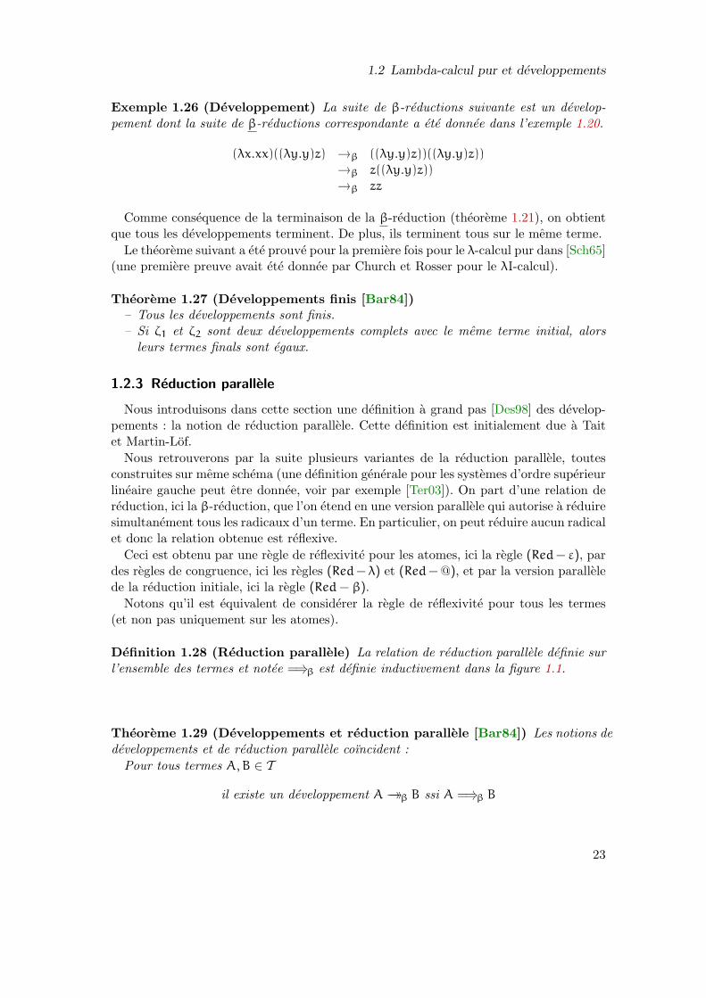
Exemple 1.26 (Developpement) La suite de β-reductions suivante est un develop-pement dont la suite de β-reductions correspondante a ete donnee dans l’exemple 1.20.
(λx.xx)((λy.y)z) →β ((λy.y)z))((λy.y)z))
→β z((λy.y)z))
→β zz
Comme consequence de la terminaison de la β-reduction (theoreme 1.21), on obtientque tous les developpements terminent. De plus, ils terminent tous sur le meme terme.
Le theoreme suivant a ete prouve pour la premiere fois pour le λ-calcul pur dans [Sch65](une premiere preuve avait ete donnee par Church et Rosser pour le λI-calcul).
Theoreme 1.27 (Developpements finis [Bar84])– Tous les developpements sont finis.– Si ζ1 et ζ2 sont deux developpements complets avec le meme terme initial, alors
leurs termes finals sont egaux.
1.2.3 Reduction parallele
Nous introduisons dans cette section une definition a grand pas [Des98] des develop-pements : la notion de reduction parallele. Cette definition est initialement due a Taitet Martin-Lof.
Nous retrouverons par la suite plusieurs variantes de la reduction parallele, toutesconstruites sur meme schema (une definition generale pour les systemes d’ordre superieurlineaire gauche peut etre donnee, voir par exemple [Ter03]). On part d’une relation dereduction, ici la β-reduction, que l’on etend en une version parallele qui autorise a reduiresimultanement tous les radicaux d’un terme. En particulier, on peut reduire aucun radicalet donc la relation obtenue est reflexive.
Ceci est obtenu par une regle de reflexivite pour les atomes, ici la regle (Red− ε), pardes regles de congruence, ici les regles (Red− λ) et (Red− @), et par la version parallelede la reduction initiale, ici la regle (Red− β).
Notons qu’il est equivalent de considerer la regle de reflexivite pour tous les termes(et non pas uniquement sur les atomes).
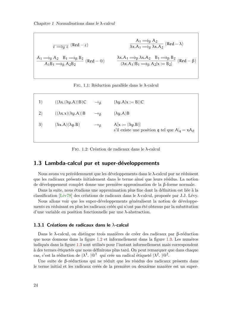
Definition 1.28 (Reduction parallele) La relation de reduction parallele definie surl’ensemble des termes et notee =⇒β est definie inductivement dans la figure 1.1.
Theoreme 1.29 (Developpements et reduction parallele [Bar84]) Les notions dedeveloppements et de reduction parallele coıncident :
Pour tous termes A,B ∈ T
il existe un developpement A→→β B ssi A =⇒β B
23
Chapitre 1 Normalisations dans le λ-calcul
ε =⇒β ε(Red− ε)
A1 =⇒β A2
λx.A1 =⇒β λx.A2(Red− λ)
A1 =⇒β A2 B1 =⇒β B2
A1B1 =⇒β A2B2(Red− @)
λx.A1 =⇒β λx.A2 B1 =⇒β B2
(λx.A1)B1 =⇒β A2[x := B2](Red− β)
Fig. 1.1: Reduction parallele dans le λ-calcul
1) ((λx.(λy.A))B)C →β (λy.A[x := B])C
2) ((λx.x)(λy.A))B →β (λy.A)B
3) (λx.A)(λy.B) →β A[x := (λy.B)]
s’il existe une position q tel que A|q = xA0
Fig. 1.2: Creation de radicaux dans le λ-calcul
1.3 Lambda-calcul pur et super-developpements
Nous avons vu precedemment que les developpements dans le λ-calcul pur ne reduisentque les radicaux presents initialement dans le terme ainsi que leurs residus. La notionde developpement complet donne une premiere approximation de la β-forme normale.
Dans la suite, nous etudions une approximation plus fine dont la definition est liee a laclassification [Lev78] des creations de radicaux dans le λ-calcul, proposee par J.J. Levy.
Nous allons voir que les super-developpements generalisent la notion de developpe-ments en reduisant en plus les radicaux crees qui n’ont pas ete obtenus par la substitutiond’une variable en position fonctionnelle par une λ-abstraction.
1.3.1 Creations de radicaux dans le λ-calcul
Dans le λ-calcul, on distingue trois manieres de creer des radicaux par β-reductionque nous donnons dans la figure 1.2 et informellement dans la figure 1.3. Les numerosindiques dans la figure 1.3 sont utilises pour l’instant informellement mais correspondenta des termes etiquetes que nous definirons plus tard. On peut remarquer que dans chaquecas, c’est la reduction de (λ1. )@1 qui cree un radical etiquete (λ2. )@2.
Une suite de β-reductions qui ne reduit que les residus des radicaux presents dansle terme initial et les radicaux crees de la premiere ou deuxieme maniere est un super-
24

1.3 Lambda-calcul pur et super-developpements
Creation de type 1
@2
;;;;
;
@1
||||
CCCC
C
λ1
λ2
→ @2
||||
;;;;
;
λ2
Creation de type 2
@2
;;;;
;
@1
|||| CC
CC
λ1WW λ2
→ @2
||||
;;;;
;
λ2
Creation de type 3
@1
KKKKKKK
rrrrrrr
λ1x
9999
9999
9999
9999
9999
λ2
@2
>>
>>
x
→
4444
4444
4444
4444
4444
@2
||||
;;;;
;
λ2
Fig. 1.3: Creation de radicaux dans le λ-calcul
25

Chapitre 1 Normalisations dans le λ-calcul
developpement. Tous les super-developpements, comme les developpements, sont finis.De plus, les creations de type 1 et 2 se font « par le haut » alors que la creation de
type 3 se fait « par le bas ». C’est precisement cette remarque qui justifie intuitivementla restriction de termes bien etiquetes definie ci-dessous.
Avant de definir le λ-calcul etiquete, nous insistons sur la difference entre la creationde radicaux de type 1 ou 2 et de type 3. Cette remarque sera utile par la suite pour definirla notion adequate de reduction parallele qui correspond aux super-developpements.
Remarque 1.30 (Creation de type 1&2 vs de type 3) Les creations de radicauxde type 1 ou 2 et de type 3 se distinguent par la remarque suivante : dans le premier casc’est la reduction du terme en position fonctionnelle de l’application etiquetee 2 qui creele radical. Dans la creation de type 3, c’est la substitution d’une variable en positionfonctionnelle par une λ-abstraction qui cree le radical.
1.3.2 Lambda-calcul etiquete
On generalise l’ensemble des termes soulignes en un ensemble de termes etiquetes. Lesetiquettes sont des entiers naturels, c’est-a-dire des elements de N.
Definition 1.31 (Termes etiquetes) Soient K un ensemble de constantes et X unensemble infini denombrable de variables. L’ensemble des termes etiquetes, note Te est
– le plus petit ensemble contenant toutes les constantes et toutes les variables– et clos par les regles suivantes :
– si A est un element de l’ensemble Te et p est un element de N alors λpx.A est unelement de Te.
– si A et B sont des elements de Te et p un element de N, alors (AB)p est unelement de Te.
Definition 1.32 (Relation de βe-reduction) La relation de βe-reduction est definiesur l’ensemble des termes etiquetes par
((λpA.)B)p →βeA[x := B]
Lorsque l’etiquette d’une application n’intervient pas dans les reductions, nous pou-vons sans ambiguıte ne pas la donner explicitement.
Pour definir la notion de super-developpements nous nous restreignons aux termes bienetiquetes, qui limite la reduction des radicaux crees « par le haut », comme remarqueprecedemment.
Definition 1.33 (Termes bien etiquetes) Un terme etiquete A de l’ensemble Te estdit bien etiquete si pour toutes positions q1 et q2 telles que A|q1
= (B0B1)p et A|q2
=
λpx.C alors necessairement q1 q2.
Il n’est pas difficile de remarquer que l’ensemble des termes bien etiquetes est clospar βe-reduction. Dans la suite, on supposera que tous les termes etiquetes sont bienetiquetes.
26

1.3 Lambda-calcul pur et super-developpements
Definition 1.34 (Termes initialement bien etiquetes) Un terme est dit initiale-ment bien etiquete :
– si c’est un terme bien etiquete ;– si pour toutes positions q1 et q2 telles que A|q1
= λpx.C et A|q2= λpx
′.C ′ alorsnecessairement q1 = q2.
Theoreme 1.35 (Normalisation forte de βe [Raa93]) La βe-reduction est termi-nante sur l’ensemble des termes etiquetes.
Theoreme 1.36 (Confluence de βe [Raa93]) La βe-reduction est confluente sur l’en-semble des termes etiquetes.
1.3.3 Super-developpements
Nous definissons tout d’abord une correspondance entre le λ-calcul avec etiquette etle λ-calcul.
Definition 1.37 (Morphisme d’effacement) Le morphisme Υ : Te → T d’efface-ment des etiquettes est defini comme suit
1. Υ(x) = x ;
2. Υ(c) = c ;
3. Υ(AB)p = Υ(A)Υ(B) ;
4. Υ(λpx.A) = λx.Υ(A).
On peut etendre le morphisme Υ a toute suite de βe-reductions, ce qui nous permetde definir la notion de super-developpements.
Definition 1.38 (Super-developpement) Une suite de β-reductions ζ du λ-calculpur est un super-developpement (aussi appele super-developpement complet) s’il existeune suite de βe-reductions σ du λ-calcul etiquete qui termine sur une βe-forme normaleet telle que Υ(σ) = ζ.
Exemple 1.39 (Super-developpement) La suite de β-reductions suivante :
(λx.λy.xy)zz ′ →β (λy.zy)z ′ →β zz ′
est un super-developpement puisqu’elle correspond a la suite de βe-reductions suivante :
(((λ1x.λ2y.xy)z)1)z ′)2 →βe
((λ2y.zy)z′)2 →βe
zz ′ .
Exemple 1.40 (Super-developpement) La suite de β-reductions suivante :
((λx.x)(λy.y))z →β (λy.y)z →β z
est un super-developpement puisqu’elle correspond a la suite de βe-reductions suivante :
(((λ1x.x)(λ2y.y))1z)2 →βe
((λ2y.y)z)2 →β z
27

Chapitre 1 Normalisations dans le λ-calcul
Exemple 1.41 (Super-developpement) La suite de β-reductions suivante :
(λx.xx)(λx.xx) →β (λx.xx)(λx.xx) →β . . .
n’est pas un super-developpement.
Essayons en effet « d’etiqueter » le terme (λx.xx)(λx.xx) et de trouver la suite de βe-reductions adequate. Nous allons voir etape par etape que nous ne pouvons pas obtenirun terme bien etiquete satisfaisant.
Commencons par etiqueter les λ-abstractions. Comme on cherche un terme initiale-ment bien etiquete, chaque λ-abstraction doit avoir une etiquette differente. Sans pertede generalite on peut supposer que l’on a les etiquettes suivantes :
(λ1x.xx)(λ2x.xx).
Pour que le terme contienne un βe-radical necessairement on doit avoir
((λ1x.xx)(λ2x.xx))1.
Pour conclure l’etiquetage de (λx.xx)(λx.xx) il nous reste a determiner les etiquettes p1
et p2 telles que le terme
((λ1x.(xx)p1 )(λ2x.(xx)
p2 ))1
soit bien etiquete. Or si on souhaite obtenir un terme reductible apres une etape deβ-reduction, alors p1 est necessairement egal a 2 ; ce qui est impossible puisque l’onsouhaite un terme bien etiquete.
Etant donne un λ-terme, on peut « l’etiqueter » d’une certaine maniere (et donc obtenirun terme etiquete) pour βe-reduire les radicaux crees de la premiere et deuxieme manieremais pas de la troisieme. C’est exactement pour cela que l’on s’est restreint aux termesbien etiquetes.
A partir de maintenant, la suite de βe-reductions associee a un super-developpementne sera pas directement explicitee. Nous pouvons remarquer de plus que comme βe estfortement normalisant et confluent alors nous pouvons parler de la βe-forme normale.
Exemple 1.42 (Radicaux et (super-)developpements) Nous donnons 4 exemplesde suite de β-reductions qui sont des super-developpements en explicitant les creationsde radicaux mise en jeu.
1. Les residus des radicaux presents dans le terme initial peuvent etre contractes.Cette suite de β-reductions est aussi un developpement.
(λx.f(x, x)) ((λy.y) a)
→β f((λy.y) a, (λy.y) a)
→β f(a, (λy.y) a)
→β f(a, a)
28

1.3 Lambda-calcul pur et super-developpements
2. La premiere reduction de la sequence suivante cree un radical (creation de type 1).Ce radical est ensuite reduit dans le super-developpement suivant :
((λx.λy.f(x, y))a)b
→β (λy.f(a, y))b
→β f(a, b)
3. Comme dans la reduction precedente, un radical est cree par reduction mais d’unemaniere differente (creation de type 2).
((λx.x)(λy.y))a
→β (λy.y)a
→β a
4. Il n’existe pas de super-developpement du terme (λx.xa)(λy.y) vers le terme a. Leseul super-developpement envisageable serait le suivant.
(λx.xa)(λy.y)
→β (λy.y)a
La creation de radical est de type 3. Le radical cree ne peut pas etre reduit parsuper-developpement.
Theoreme 1.43 (Super-developpements finis [Raa96])– Tous les super-developpements sont finis.– Si ζ1 et ζ2 sont deux super-developpements complets avec le meme terme initial,
alors leurs termes finals sont egaux.
1.3.4 Reduction parallele forte
On peut generaliser la notion de reduction parallele (qui coıncide avec la notion dedeveloppements) pour obtenir de la meme maniere une correspondance avec la notion desuper-developpements. Historiquement, la notion de reduction parallele forte introduitedans [Acz78] apparaıt anterieurement a la notion de super-developpements.
Definition 1.44 (Reduction parallele forte) La reduction parallele forte definie surl’ensemble des termes T et notee =⇒βf
est la plus petite relation close par les reglesdonnee dans la figure 1.4.
Nous disons simplement que le terme A se βsd-reduit sur le terme B s’il existe unsuper-developpement entre A et B. Dans la definition de la reduction parallele forte, laregle (Red-βf) est venue remplacer la regle (Red-β) de la reduction parallele, differencesignificative qui fait passer des developpements aux super-developpements.
La regle (Red-βf) reduit le radical forme a partir de la λ-abstraction donnee par lereduit du terme A1. Cette λ-abstraction a donc bien ete obtenue apres reduction de A1
(par opposition a la regle (Red-β) qui reduit le radical present dans le terme initial). Leradical ainsi reduit par la regle n’etait donc pas necessairement present dans le termeinitial A1A2. Il a donc ete eventuellement cree par reduction.
29

Chapitre 1 Normalisations dans le λ-calcul
ε =⇒βfε (Red− ε)
A1 =⇒βfA2
λx.A1 =⇒βfλx.A2
(Red− λ)
A1 =⇒βfA2 B1 =⇒βf
B2
A1B1 =⇒βfA2B2
(Red− @)A1 =⇒βf
λx.A2 B1 =⇒βfB2
A1B1 =⇒βfA2[x := B2]
(Red− βf)
Fig. 1.4: Reduction parallele forte dans le λ-calcul
Definition 1.45 (βsd-forme normale) La βsd-forme normale d’un terme A est leterme B tel que
1. A =⇒βfB
2. il n’existe pas de terme B ′ 6= B tel que A =⇒βfB ′ et B =⇒βf
B ′.
La βsd-forme normale est obtenue en appliquant prioritairement la regle (Red-βf). Laremarque 1.30 sur la difference entre les differentes creations de radicaux conduit autheoreme suivant.
Theoreme 1.46 (Super-developpements et reduction parallele forte [Raa96])Pour tous termes A et B de l’ensemble T
il existe un super-developpement A→→β B ssi A =⇒βfB
Du theoreme precedent et de la confluence de βe on en deduit que la relation =⇒βf
verifie la propriete du diamant.
Propriete 1.47 (Propriete du diamant pour =⇒βf) Soient A,B,C des termes de
T . Si A =⇒βfB et A =⇒βf
C alors il existe un terme D tel que B =⇒βfD et C =⇒βf
D.
Aβf
βf
#@@
@@@@
@
@@@@
@@@
B
βf #?
??
?
??
?? C
βf ~~
~~
~~
~~
D
Conclusion
Le materiel de base introduit dans ce chapitre sera utilise tout au long de la premierepartie de cette these. Nous allons voir que les super-developpements conduisent a unenouvelle approche pour le filtrage d’ordre superieur.
30
Chapitre 2
Filtrage d’ordre superieur
Contexte L’egalite de deux termes modulo β est un probleme indecidable dans le λ-calcul, comme l’a montre Church. L’unification et le filtrage dans le λ-calcul pur nepeuvent donc pas etre etudier directement puisqu’ils necessitent de decider de l’egalitede deux termes. Neanmoins, en pratique on n’a pas besoin de toute la puissance duλ-calcul pur et dans le cadre de la deduction automatique par exemple on etudie l’uni-fication dans le cadre du λ-calcul simplement type (isomorphisme de Curry-Howard-deBruijn). L’unification reste dans ce contexte toujours indecidable [Hue76] mais commel’a montre D. Miller dans [Mil91] les termes que l’on ecrit en pratique verifient souventdes contraintes qui font que l’unification devient decidable et peut meme etre resolue entemps lineaire [Qia96].
Le travail presente ici concerne le filtrage d’ordre superieur qui requiert une etudeparticuliere bien qu’etant un cas particulier de l’unification (voir par exemple [HL78]).Il est utilise principalement pour la reecriture d’ordre superieur [KOR93, MN98, Ter03,BCK06] et pour la transformation de programmes [MS01, Hag90, HM88, HL78]. Nean-moins, les algorithmes utilises sont souvent une specialisation de l’algorithme generald’unification tel qu’il a ete introduit dans [Hue76] et sont complexes a comprendre etmettre en œuvre.
Contributions Nous proposons dans ce chapitre et le chapitre suivant une approchenouvelle au filtrage d’ordre superieur. Au lieu de decider de l’egalite modulo β dans leλ-calcul type, nous proposons de considerer une restriction decidable de la β-equivalencedans un cadre non type. Cette restriction est donnee par les super-developpements quiont ete introduits au chapitre 1.
Elle peut paraıtre arbitraire et restrictive mais remarquablement, l’approximation don-nee par les super-developpements coıncide avec la β-forme normale pour les termesdu second-ordre. Autrement dit, l’ensemble des filtres modulo super-developpementscontient les filtres du second-ordre. Ceci est particulierement important puisqu’en pra-tique, les problemes que l’on considere sont tres souvent du second ordre. Nous mon-trons aussi que les super-developpements sont suffisamment expressifs pour traiter lesproblemes de filtrage sur des motifs a la Miller.
Le filtrage d’ordre superieur dans un cadre non type a ete etudie pour la premierefois dans [Sit01, MS01]. Les equations de filtrage sont resolus modulo une reductionatomique (une etape) qui ne coıncident pas avec la notion de reduction parallele deTait and Martin-Lof. Elle termine neanmoins et fournit une approximation a l’operation
31

Chapitre 2 Filtrage d’ordre superieur
de β-normalisation. La reduction atomique consideree est comme l’indique les auteursdu papier original, difficile a comprendre. La theorie des super-developpements donnedes intuitions claires et un cadre formel solide permettant une comparaison simple avecles autres approches du filtrage d’ordre superieur. Les preuves par rapport aux travauxinitiaux [Sit01, MS01] sont considerablement simplifiees.
Nous verrons dans le chapitre suivant que l’algorithme et les concepts pour le fil-trage modulo super-developpements etant clarifies, il est maintenant simple de deduireplusieurs proprietes et variantes de cet algorithme. En particulier, nous obtenons un al-gorithme original pour le filtrage du second-ordre et des proprietes de minimalite dansle cadre des motifs a la Miller.
Les principales idees de ce chapitre et du suivant ont ete presentees dans [Fau06]. Uneversion detaillee proche de la presentation donnee ici est disponible dans [Fau07].
Plan du chapitre Dans une section preliminaire, nous introduisons les variables de fil-trage qui seront les inconnues des equations que nous allons resoudre. Nous definissonsensuite le filtrage d’ordre superieur dans le λ-calcul simplement type (modulo β sec-tion 2.1.1 et modulo βη section 2.1.3) et le filtrage modulo super-developpements dansle λ-calcul pur (section 2.2.1 et section 2.2.5 avec η). Nous comparons ce dernier avec dif-ferentes instances du filtrage dans le λ-calcul simplement type : filtrage du second ordre(section 2.2.2), du troisieme ordre (section 2.2.3) et des motifs a la Miller (section 2.2.4).
Variables de filtrage
En general, une equation de filtrage est definie par la donnee d’un couple de termes.Un des deux termes est clos. Les variables libres de l’autre terme sont les inconnuesdu probleme de filtrage, c’est-a-dire les variables que l’on cherche a instancier afin derendre les deux termes egaux modulo une equivalence donnee (traditionnellement, pourle λ-calcul simplement type, la βη-equivalence).
Nous proposons une presentation legerement differente, ou les inconnues appartiennenta un ensemble separe. Autrement dit, dans toute la suite du chapitre, aussi bien dans lecadre type que non type, nous supposerons donnes deux ensembles disjoints de variables :l’ensemble X defini comme dans le chapitre 1 et l’ensemble V, appele ensemble desvariables de filtrage et qui representent les inconnues.
Les variables de filtrage seront denotees par les lettres X, Y, Z . . .. Elles ne peuventpas etre liees par une λ-abstraction. Elles seront substituees durant la resolution d’unprobleme de filtrage. Dans le cadre type, chaque variable de filtrage a un type donne etnous supposerons que V peut etre partitionne en des ensembles disjoints de variables defiltrage d’un type donne.
Ainsi l’ensemble des termes (non types) est defini par
32

A,B ::= x (Variable)| X (Variable de filtrage)| c (Constante)| λx.A (Abstraction)| A B (Application)
Afin de lever toute ambiguıte, nous rappelons la definition des variables libres poursouligner qu’elle ne concerne pas les variables de filtrage.
Definition 2.1 (Variables libres et liees) L’ensemble des variables libres d’un termeA note fv(A) et l’ensemble des variables liees note bv(A) sont definis par
fv(x) = x bv(x) = ∅fv(X) = ∅ bv(X) = ∅fv(a) = ∅ bv(a) = ∅
fv(AB) = fv(A) ∪ fv(B) bv(AB) = bv(A) ∪ bv(B)
fv(λx.A) = fv(A)\x bv(λx.A) = bv(A) ∪ x
Definition 2.2 (Terme X -clos et terme V-clos) Un terme A est dit X -clos s’il necontient pas de variable libre, c’est-a-dire si fv(A) = ∅.
Un terme est dit V-clos s’il ne contient pas de variable de filtrage.
Definition 2.3 (Substitution) Une substitution de variables de filtrage ou plus sim-plement une substitution est une fonction de l’ensemble des variables de filtrage dansl’ensemble des termes V-clos (types ou non suivant le contexte). La substitution de lavariable de filtrage X par A dans B est denotee par BA/X.
Si l’on avait utilise la terminologie des CRS [Klo80, KOR93], on aurait appele « meta-variables » les variables de filtrage, « meta-termes » les termes contenant eventuellementdes variables de filtrage et « termes » nos termes V-clos. Les substitutions des variablesde filtrage pour des termes V-clos correspondent bien aux « assignement » des CRS.
Dans ce chapitre, nous ne considerons que des substitutions normales, c’est-a-dire dessubstitutions de termes normaux. Nous notons par id la substitution identite (aussiappelee substitution vide).
Comme nous considerons les termes modulo α-conversion, lorsque l’on applique unesubstitution de variable de filtrage, un representant adequat est choisi pour eviter d’even-tuelles captures de variables.
De la meme maniere qu’il existe une injection canonique de l’ensemble des termestypes dans l’ensemble des termes, il existe une injection canonique des substitutionsdefinies sur les termes types Tt dans l’ensemble des substitutions definies sur l’ensembledes termes non types T . Cette injection ne sera pas explicitement indiquee.
Definition 2.4 (Domaine, co-domaine) Si φ = A1/X1, . . . , An/Xn est une substi-tution alors son domaine est l’ensemble Xi
ni=1 et son co-domaine est l’ensemble Ai
ni=1.
33
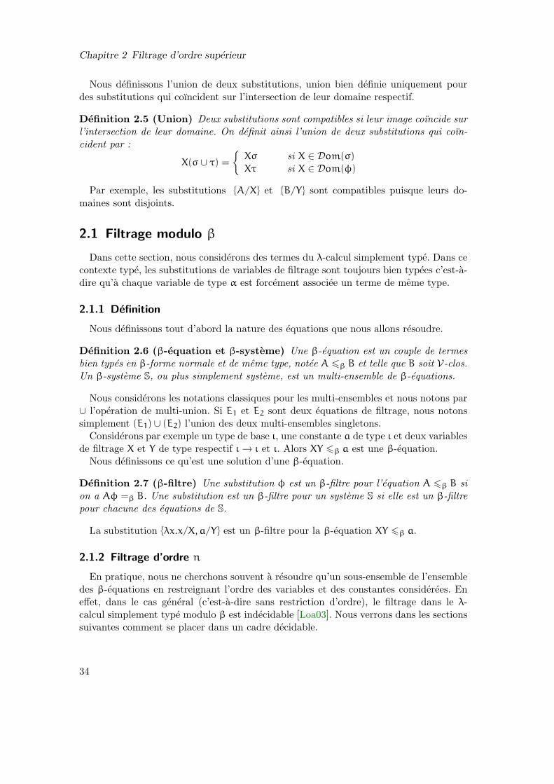
Chapitre 2 Filtrage d’ordre superieur
Nous definissons l’union de deux substitutions, union bien definie uniquement pourdes substitutions qui coıncident sur l’intersection de leur domaine respectif.
Definition 2.5 (Union) Deux substitutions sont compatibles si leur image coıncide surl’intersection de leur domaine. On definit ainsi l’union de deux substitutions qui coın-cident par :
X(σ ∪ τ) =
Xσ si X ∈ Dom(σ)
Xτ si X ∈ Dom(φ)
Par exemple, les substitutions A/X et B/Y sont compatibles puisque leurs do-maines sont disjoints.
2.1 Filtrage modulo β
Dans cette section, nous considerons des termes du λ-calcul simplement type. Dans cecontexte type, les substitutions de variables de filtrage sont toujours bien typees c’est-a-dire qu’a chaque variable de type α est forcement associee un terme de meme type.
2.1.1 Definition
Nous definissons tout d’abord la nature des equations que nous allons resoudre.
Definition 2.6 (β-equation et β-systeme) Une β-equation est un couple de termesbien types en β-forme normale et de meme type, notee A 6β B et telle que B soit V-clos.Un β-systeme S, ou plus simplement systeme, est un multi-ensemble de β-equations.
Nous considerons les notations classiques pour les multi-ensembles et nous notons par∪ l’operation de multi-union. Si E1 et E2 sont deux equations de filtrage, nous notonssimplement (E1) ∪ (E2) l’union des deux multi-ensembles singletons.
Considerons par exemple un type de base ι, une constante a de type ι et deux variablesde filtrage X et Y de type respectif ι→ ι et ι. Alors XY 6β a est une β-equation.
Nous definissons ce qu’est une solution d’une β-equation.
Definition 2.7 (β-filtre) Une substitution φ est un β-filtre pour l’equation A 6β B sion a Aφ =β B. Une substitution est un β-filtre pour un systeme S si elle est un β-filtrepour chacune des equations de S.
La substitution λx.x/X, a/Y est un β-filtre pour la β-equation XY 6β a.
2.1.2 Filtrage d’ordre n
En pratique, nous ne cherchons souvent a resoudre qu’un sous-ensemble de l’ensembledes β-equations en restreignant l’ordre des variables et des constantes considerees. Eneffet, dans le cas general (c’est-a-dire sans restriction d’ordre), le filtrage dans le λ-calcul simplement type modulo β est indecidable [Loa03]. Nous verrons dans les sectionssuivantes comment se placer dans un cadre decidable.
34
2.1 Filtrage modulo β
Definition 2.8 (Ordre d’un systeme) Une β-equation est dite d’ordre au plus n sitoutes ses inconnues sont d’ordre au plus n et si toutes ses constantes sont d’ordre auplus n+ 1. Un systeme est dit d’ordre au plus n s’il est compose d’equations d’ordre auplus n.
Par exemple, la β-equation XY 6β a est d’ordre 2.
Definition 2.9 (Filtrage d’ordre n modulo β) Nous designons par filtrage d’ordren modulo β la recherche des β-filtres de β-systemes d’ordre au plus n.
2.1.3 Filtrage modulo βη
En pratique l’egalite qui est interessante est non pas l’egalite modulo β mais l’egalitemodulo βη c’est-a-dire que l’on rajoute dans la theorie equationnelle l’equation
(η) λx.(Ax) = A
si x 6∈ fv(A)
La complexite du filtrage modulo βη a ete abondamment etudiee. Sa decidabilite estrestee un probleme ouvert pendant plus de trente ans (conjecturee dans [Hue76]). Ladecidabilite a l’ordre 2 est etabli dans [HL78], a l’ordre 3 dans [Dow94] et a l’ordre 4dans [Pad00]. La preuve de decidabilite generale (sans restriction d’ordre) n’apparaıt quedans les recents travaux de [Sti06] utilisant la theorie des jeux.
Nous reformulons les definitions donnees precedemment modulo βη.
Definition 2.10 (βη-equation et βη-systeme) Une βη-equation est un couple de λ-termes bien types en forme normale η-longue et de meme type, notee A 6βη B et telleque B soit V-clos. Un βη-systeme S est un multi-ensemble de βη-equations.
Definition 2.11 (βη-filtre) Une substitution φ est un βη-filtre pour l’equation A 6βη
B si on a Aφ =βη B. Une substitution est un βη-filtre pour un systeme S si elle est unβη-filtre pour chacune des equations de S.
2.1.4 Filtrage de motifs a la Miller
Nous definissons tout d’abord l’ensemble de motifs a la Miller.
Definition 2.12 (Motifs a la Miller) Un λ-terme type A en β-forme normale est unmotif a la Miller si chaque occurrence d’une variable de filtrage est dans un sous-termeX(A1, . . . , An) de A tel que (A1, . . . , An) soit η-equivalent a une liste de variables lieesdistinctes.
Par opposition a l’unification d’ordre superieur qui est indecidable en generale [Hue73,Hue75, Gol81], l’unification de motifs a la Miller est decidable. De plus, quand un pro-bleme a une solution, il en existe une plus generale. La recherche de cette solution laplus generale peut etre faite en un temps lineaire [Qia96]. Nous montrerons dans la sec-tion 3.2.2 que l’algorithme propose pour le filtrage modulo super-developpements et ηdonne exactement (et uniquement) le filtre le plus general pour toute equation ayant unesolution.
35
Chapitre 2 Filtrage d’ordre superieur
2.2 Filtrage modulo super-developpements
2.2.1 Definition
Nous considerons dans cette section des termes du λ-calcul pur, c’est-a-dire des ele-ments de T . Nous allons considerer la resolution d’equations modulo la restriction de laβ-reduction donnee par les super-developpements qui a ete introduite au chapitre 1.
Nous definissons comme dans la section precedente, tout d’abord la notion d’equationdans ce contexte. Ensuite, nous definissons ce que ce sont les solutions de telles equations.
Definition 2.13 (βsd-equation et βsd-systeme) Une βsd-equation est un couple determes denotee A 6βsd
B,telle que B est V-clos et en β-forme normale. Un βsd-systemeS, ou plus simplement systeme, est un multi-ensemble (eventuellement vide) de βsd-equations.
On dit que la variable de filtrage X appartient a un systeme S et on note X ∈ S si cettevariable apparaıt dans une des equations du systeme S.
Exemple 2.14 (βsd-equations) Par exemple, le couple (XY, λx.x) ainsi que le couple((λx.x)X, a) sont des βsd-equations de filtrage alors que le couple (XY, (λx.x)a) n’en estpas une puisque le terme (λx.x)a n’est pas en forme normale.
Comme l’indique l’exemple precedent, contrairement aux β-equations, le terme Ad’une βsd-equation A 6βsd
B n’est pas suppose en forme normale, ce que nous jus-tifierons dans la section 3.1 (paragraphe sur les regles (ε)).
Definition 2.15 (βsd-filtre) Une substitution φ est un βsd-filtre pour A 6βsdB s’il
existe un super-developpement entre Aφ et B (soit Aφ =⇒βfB). Une substitution est
un βsd-filtre pour un systeme S si elle est un βsd-filtre pour chacune des equations quiconstituent S. L’ensemble des filtres d’un systeme S est note M(S).
De la meme maniere que l’on peut associer a tout terme type un terme non type, onpeut associer a chaque β-equation une βsd-equation. Par abus de notation, nous noteronssimplement A 6βsd
B la βsd-equation associee a la β-equation A 6β B.Rappelons que nous ne considerons que des substitutions normales et closes c’est-a-
dire des substitutions de termes clos et normaux. En particulier un βsd-filtre est doncbien une substitution normale et close.
Exemple 2.16 (βsd-filtres) Considerons l’equation
XY 6βsdλx.x.
– Les substitutions
σ1 = λx.λy.y/X et σ2 = λy.y/X, λx.x/Y
sont des βsd-filtres pour cette equation puisque
(XY)σ1 = (λx.λy.y)Y =⇒βfλx.x et (XY)σ2 = (λy.y)(λx.x) =⇒βf
λx.x.
36

2.2 Filtrage modulo super-developpements
– La substitution
λz.z(λx.x)/X, λy.y/Y
n’est pas un βsd-filtre puisque
(λz.z(λx.x))(λy.y) 6=⇒βfλx.x
bien que ces deux-termes soient β-convertibles.– La substitution
σ3 = (λy.y)(λz.z)/X, λx.x/Y
n’est pas un βsd-filtre puisqu’elle n’est pas normale.
Nous allons voir qu’une equation peut avoir un nombre infini de βsd-filtres, qu’iln’existe pas de filtre plus general mais qu’il existe toujours une partie generatrice (pro-position 3.14).
Exemple 2.17 (Nombre infini de βsd-filtres) Nous continuons l’exemple 2.16. Nouspouvons remarquer que de la meme maniere que
σ1 = λx.λy.y/X
est un βsd-filtre pour l’equation XY 6βsdλx.x, toutes les substitutions qui sont compa-
tibles avec σ1 sont aussi solutions, quelle que soit la valeur associee a Y (il y en a doncune infinite). Nous pouvons citer par exemple les substitutions
σ2 = λx.λy.y/X, λx.x/Y et σ3 = λx.λy.y/X, λx.λy.y/Y.
Ces deux substitutions seront « representees » par la substitution σ1 dans le sens ou :
σ1 ≤ σ2 et σ1 ≤ σ3
Par contre, il n’existe pas de filtre plus general comme le montre l’exemple suivant.
Exemple 2.18 (βsd-filtres incomparables) Nous continuons encore l’exemple 2.16.Une autre solution de l’equation consideree est donnee par
σ4 = λx.λy.x/X, λx.x/Y.
Les deux substitutions σ1 et σ4 sont incomparables.
Nous cherchons a resoudre des βsd-equations. Pour cela, nous allons transformer paretapes successives [MM82, Kir84] un systeme jusqu’a obtenir un systeme a partir duquelon peut extraire facilement un βsd-filtre (s’il existe). Un tel systeme est un systeme diten forme resolue dans le sens de la definition suivante.
37

Chapitre 2 Filtrage d’ordre superieur
Definition 2.19 (Forme resolue) Une equation X 6βsdA est en forme resolue si le
terme A est X -clos. La substitution associee a une telle equation est definie par A/X.Un systeme est en forme resolue si chacune des equations qui le constituent sont
en forme resolue et si les membres gauches des equations etant deux a deux disjoints.La substitution associee a un systeme resolu S est l’union des substitutions associees achacune des equations. Elle est denotee σS.
Si le systeme est le multi-ensemble vide alors la substitution associee est la substitutionidentite.
La substitution associee a un systeme resolu est bien definie puisque c’est l’union desubstitutions qui sont compatibles deux a deux (elles sont compatibles puisque leursdomaines sont disjoints, les membres gauches des equations etant deux a deux disjoints).
Nous allons donner dans la section 3.1 un algorithme pour la recherche des βsd-filtres.Or, il peut exister un nombre infini de βsd-filtres (exemple 2.17) et il n’existe pas de plusgeneral filtre (exemple 2.18). C’est pour cela que nous introduisons la notion d’ensemblecomplet de filtres. Nous prouverons dans la proposition 3.14 que dans le cas du filtragemodulo super-developpements dans le λ-calcul pur, si une equation a une solution alorsil existe toujours un ensemble complet fini de filtres.
Definition 2.20 (Ensemble complet de filtres) Soit S un ensemble d’equations. Unensemble complet de filtre pour S est un ensemble de substitutions M de domaine inclusdans les variables de filtrage de S et tel que
1. Correction Pour toutes les substitutions φ ∈ M, φ est un βsd-filtre de S ;
2. Completude Pour toutes les substitutions φ telle que φ est un βsd-filtre pour S,il existe ψ ∈ M telle que ψ ≤ φ c’est-a-dire qu’il existe une substitution ψ telleque φ = ξ ψ ou denote la composition de substitution.
Lemme 2.21 (Correction des formes resolues) Si un systeme S est en forme re-solue alors σS est un ensemble complet de filtre pour S.
2.2.2 Comparaison avec le filtrage du second ordre
Nous avons vu qu’a toute β-equation correspond une βsd-equation. En nous restrei-gnant a des β-equations d’ordre au plus 2, nous allons montrer que tout β-filtre d’unetelle equation est un βsd-filtre pour la βsd-equation correspondante.
Nous avons decrit dans le chapitre 1, les trois manieres de creer un radical dans le λ-calcul. La troisieme maniere induit l’existence dans le terme initial d’un radical d’ordreau moins 3. Nous rappelons tout d’abord que les super-developpements reduisent tousles radicaux residus de radicaux presents dans le terme initial et tous les radicaux creesqui ne l’ont pas ete par la troisieme maniere. Or, si l’on considere une β-equation dusecond ordre, il n’y aura jamais de radical d’ordre au moins 3 et donc jamais de creationde radical de type 3. Autrement dit, dans ce contexte, la β-forme normale et la βsd-forme normale coıncident et donc tout β-filtre est un βsd-filtre. C’est ce que nous allonsformaliser dans la suite de cette section.
Nous commencons par un lemme technique sur la creation de radicaux.
38

2.2 Filtrage modulo super-developpements
Lemme 2.22 (Ordre d’un radical et super-developpements) Soient A1, . . .An−1
et An des termes types. Supposons de plus que An contienne un radical d’ordre au moins3 et qu’il existe un super-developpement A1→β . . .→β An. Alors A1 contient aussi unradical d’ordre au moins 3.
Preuve. Nous prouvons le resultat par induction sur n. Le resultat est vrai dans le cas debase (n = 1). Supposons maintenant que le resultat est vrai pour n. On veut le prouverpour n + 1. Par hypothese d’induction, nous savons que A2 contient un radical d’ordreau moins 3 que nous denoterons par la suite par R = (λx.C)D. Nous raisonnons par cassuivant suivant que R est un residu ou a ete cree durant la reduction de A1 en A2 enanalysant les trois manieres dont il a pu etre cree.
– Si R est le residu d’un radical de A1 alors le resultat est vrai.– Sinon, c’est-a-dire si le radical R est cree durant la reduction de A1 en A2 de la
premiere maniere alors le terme A1 contient necessairement un sous-terme de laforme (((λz.λx.C ′) E)D avec C = C ′[z := E]. L’ordre du radical (λz.λx.C ′) E est aumoins celui de R. Ce qui conclut le cas.
– Sinon, c’est-a-dire si R est cree durant la reduction de A1 en A2 de la deuxiememaniere alors A1 doit contenir un sous-terme de la forme (λy.y) (λx.C)D. L’ordredu radical (λy.y) (λx.C) est strictement superieur a l’ordre de R. Ce qui conclut lecas.
– Sinon, c’est-a-dire si R est cree durant la reduction de A1 en A2 de la troisiememaniere alors A1 doit contenir un sous-terme de la forme R ′ = (λz.E)(λx.C) et ilexiste une position q telle que E|q = zD ′ avec D = D ′[z := λx.C]. L’ordre du radicalR ′ est strictement superieur a l’ordre de R. Ce qui conclut le cas.
Propriete 2.23 (Super-developpements et second ordre) Si φ est un β-filtre pourune β-equation du second ordre alors φ est un βsd-filtre pour la βsd-equation correspon-dante.
Preuve. Raisonnons par l’absurde. Supposons qu’il existe une substitution φ qui soitun β-filtre de l’equation du second ordre A 6β B et qui ne soit pas un βsd-filtre dela βsd-equation correspondante. En d’autres termes, A ne contient aucun radical, φ necontient aucun terme d’ordre superieur a deux et Aφ =β B et Aφ 6=⇒βf
B. Il existe doncune suite (Ai)i telle que Aφ →β A1→β . . . →β An et An contient un radical (λx.C)D
qui ne peut pas etre reduit dans le super-developpement ci-dessus. C’est donc un residud’un radical cree en reduisant Ai0 (i0 entre 1 et n). Comme il n’existe pas de β-sequencequi soit un super-developpement et qui permette de reduire ce radical, la creation est detype 3 et induit donc un radical d’ordre au moins 3. Le lemme 2.22 implique que Aφcontient un radical d’ordre au moins 3. Mais comme A et φ appartiennent a l’ensembledes formes β-normales, il existe une position q de A et un terme E telle que A|q = XE
ou X est une variable de filtrage envoyee par φ sur une λ-abstraction d’ordre au moins3, ce qui contredit l’hypothese sur l’ordre de l’equation initiale.
39

Chapitre 2 Filtrage d’ordre superieur
La proposition precedente se generalise aux systemes.
Propriete 2.24 (Super-developpements et second ordre) Nous supposons donneun β-systeme du second ordre. Si φ est un β-filtre pour ce β-systeme alors φ est unβsd-filtre pour le βsd-systeme correspondant.
Preuve. Consideronns le β-systeme du second ordre
(A1 6β B1) ∪ . . . ∪ (An 6β Bn).
Dire que φ est un β-filtre pour ce systeme est equivalent a dire que φ est un β-filtrepour la β-equation
λx.x(A1, . . . , An) 6β λx.x(B1, . . . , Bn)
ou la variable x est du type adequat et x(A1, . . . , An) denote le terme (. . . (xA1) . . .).En appliquant la proposition precedente, on obtient que φ est un βsd-filtre pour laβsd-equation
λx.x(A1, . . . , An) 6βsdλx.x(B1, . . . , Bn)
ce qui est equivalent a dire que φ est un βsd-filtre pour le βsd-systeme
(A1 6βsdB1) ∪ . . . ∪ (An 6βsd
Bn).
2.2.3 Comparaison avec le filtrage du troisieme ordre
Des que l’on considere des problemes de filtrage du troisieme ordre, l’ensemble dessolutions minimales est potentiellement infini. Comme le filtrage modulo les super-developpements ne genere qu’un nombre fini de solutions minimales (resultat demontredans la proposition 3.14), on en deduit que le filtrage modulo les super-developpementsne peut pas etre complet par rapport au filtrage du troisieme ordre.
Nous exhibons donc un exemple de β-equation qui contient des inconnues d’ordre 3et qui admet une substitution qui est un β-filtre mais qui n’est pas un βsd-filtre. Pourtrouver un tel exemple il suffit de trouver deux termes bien types dont la preuve de β-egalite necessite de reduire un radical cree de la troisieme maniere. De ces deux termes,nous extrayons ensuite une equation.
Nous allons voir que l’equation consideree est du troisieme ordre et admet [Dow01] unnombre infini de solutions minimales de type ι → (ι → ι) → ι qui sont exactement lesnombres de Church λx.λf.(f . . . (f x) . . .).
Exemple 2.25 (Super-developpement et troisieme ordre) Considerons la suite deβ-reductions suivante :
40
2.2 Filtrage modulo super-developpements
λz.((λx.λf.fx) z (λy.y)) →β λz.((λf.fz)λy.y)
→β λz.((λy.y)z)
→β λz.z
On peut remarquer que la derniere etape de reduction reduit un radical cree de latroisieme maniere. Donc ce radical ne peut pas etre reduit par βsd-reduction. On endeduit que la substitution λx.λf.fx/X est un β-filtre mais n’est pas un βsd-filtre pourl’equation λz.(X z (λy.y)) ≪ λz.z.
2.2.4 Comparaison avec le filtrage des motifs a la Miller
Nous allons prouver dans cette section, que la restriction de la β-reduction donnee parles super-developpements est suffisante pour le filtrage de motifs a la Miller.
D. Miller souligne que pour les motifs a la Miller, il suffit de considerer une restrictionde la β-reduction [Mil91], appelee β0-reduction, et definie par
(λx.M)x →β0M
que l’on peut exprimer encore
(λy.M)x →β0M[y := x]
Nous avons remarque dans le chapitre 1 qu’une creation de radical de type 2 ou 3 necessitela reduction d’un radical dont le terme en position applicative est une λ-abstraction.Comme la β0-reduction ne permet de reduire que les radicaux dont le terme en positionapplicative est une variable, les seules creations de radicaux par β0-reduction sont detype 1. Les radicaux crees de la premiere maniere etant reduit par super-developpements,on a le resultat suivant :
Propriete 2.26 (Motifs a la Miller et super-developpements) Si P un motif a laMiller et si φ un β-filtre pour l’equation P 6β A alors il existe un super-developpementPφ→→β A. La substitution φ est donc un βsd-filtre pour cette equation.
2.2.5 Filtrage modulo super-developpements et η
Dans le λ-calcul simplement type, la difference technique entre le filtrage d’ordre supe-rieur modulo β et le filtrage d’ordre superieur modulo βη est principalement expliqueepar l’utilisation fondamentale de la forme normale η-longue. Cette difference est cru-ciale puisque l’utilisation de la regle η dans le filtrage permet de passer d’un problemeindecidable [Loa03] a un probleme decidable [Sti06].
Dans le contexte du filtrage d’ordre superieur modulo les super-developpements, l’uti-lisation de η n’influence ni fondamentalement ni techniquement le filtrage comme nousle montrons dans la section 3.2 en proposant un algorithme directement inspire de l’al-gorithme modulo super-developpements (sans η).
41

Chapitre 2 Filtrage d’ordre superieur
Dans le cadre type, nous considerons des termes en formes normale η-longue. Dans uncontexte non type, nous allons au contraire considerer des termes en forme η-normalec’est-a-dire, des termes en forme normale par rapport a la η-reduction definie par
λx.(Ax) →η A
si x 6∈ fv(A)
Definition 2.27 (βsdη-equation et βsdη-systeme) Une βsdη-equation de filtrage estdefinie comme un couple (A,B) de termes telle que B est βη-normal et V-clos. On de-note une telle equation par A 6βsdη B. Un βsdη-systeme est un multi-ensemble deβsdη-equations.
Definition 2.28 (βsdη-filtre) On dit qu’une substitution φ est un βsdη-filtre pour laβsdη-equation A 6βsdη B s’il existe un terme C tel que Aφ =⇒βf
C→→η B.
Ces deux notions seront illustrees dans la section 3.2.
Conclusion
Nous avons defini dans ce chapitre le filtrage modulo super-developpements et nousl’avons compare avec differentes instances du filtrage dans le λ-calcul simplement type.Dans le chapitre suivant, nous allons donner differents algorithmes implementant cesdeux approches et et montrer leur correction et completude.
42

Chapitre 3
Algorithmes de filtrage d’ordre superieur
Contributions Apres avoir defini dans le chapitre precedent le filtrage modulo β(η) etmodulo super-developpements (η), nous donnons ici plusieurs algorithmes.
Nous presentons et etudions tout d’abord un algorithme pour le filtrage modulo super-developpements. Cet algorithme presente par des regles de transformations [MM82,Kir84, SG89, JK91] est deduit de la definition de la reduction parallele forte (qui coın-cident avec les super-developpements). Nous etudions en detail les proprietes de cetalgorithme : terminaison, correction et completude.
Ensuite, nous proposons plusieurs variantes de cet algorithme qui aboutissent respecti-vement a un algorithme original pour le filtrage du second-ordre (approche differente decelle de Huet et Lang) et a un algorithme pour le filtrage modulo super-developpementset η qui, dans le cadre du filtrage de motifs a la Miller, donne (s’il existe) le filtreprincipal.
Plan du chapitre Dans la premiere section qui est le cœur de ce chapitre, nous don-nons et etudions un algorithme pour le filtrage modulo super-developpements. Dans ladeuxieme section, nous donnons deux algorithmes pour le filtrage d’ordre 2. Le premierest du a Huet et Lang et le deuxieme est directement inspire de l’algorithme pour le fil-trage modulo super-developpements de la premiere section. La troisieme section proposeun algorithme pour le filtrage modulo super-developpements et η.
3.1 Filtrage modulo super-developpements
Nous presentons dans cette section un algorithme pour le filtrage modulo super-developpements dans le λ-calcul pur. Nous l’illustrons sur des exemples. Ensuite nousetudions ses differentes proprietes.
3.1.1 Regles
Les regles pour le filtrage modulo super-developpements est donne dans la figure 3.1en utilisant des regles de transformations [MM82, Kir84, SG89, JK91]. Nous entendonspar regles de transformations des regles de reecriture qui ne sont appliquees qu’en tete.Ainsi,
– un systeme est transforme par etapes successives jusqu’a obtenir une forme normale(l’ensemble des regles est terminant) ; cette forme normale peut etre une forme
43

Chapitre 3 Algorithmes de filtrage d’ordre superieur
(A1B1 6βsdA2B2) ∪ S →@@
(A1 6βsdA2) ∪ (B1 6βsd
B2) ∪ S
(A1B1 6βsdC) ∪ S →@π
(A1 6βsdλx.C) ∪ S
ou x variable fraıche
(A1B1 6βsdC) ∪ S →@β
(A1 6βsdλx.A2) ∪ (B1 6βsd
B2) ∪ S
ou A2[x := B2] = C
et x variable fraıche, x ∈ fv(A2)
et A2, B2 β-normaux
(λx.A 6βsdλx.B) ∪ S →λλ
(A 6βsdB) ∪ S
(x 6βsdx) ∪ S →εv S
(a 6βsda) ∪ S →εc S
(X 6βsdA) ∪ S →εX
(X 6βsdA) ∪ SA/X
si fv(A) = ∅ et X ∈ S
Fig. 3.1: Regles pour le filtrage d’ordre superieur modulo super-developpements
44

3.1 Filtrage modulo super-developpements
resolue qui donne une solution au probleme de filtrage considere (l’algorithme estcorrect) ;
– en explorant toutes les reductions (l’application des regles est non-deterministe dansle sens ou deux reductions d’un meme systeme peuvent donner deux formes nor-males distinctes) et en collectant toutes les formes normales resolues, on obtient unensemble complet de filtres (l’algorithme est correct et complet).
Nous notons S → S′ s’il existe une des regles de transformation de la figure 3.1 qui
s’applique et qui permet de transformer S en S′. Nous notons egalement S→→ S
′ s’il existen > 0 systemes S1, . . . ,Sn tels que S = S1 → . . . → Sn = S
′. L’algorithme de filtragemodulo super-developpements est base sur l’equivalence entre super-developpements etreduction parallele forte. Nous analysons chaque regle de transformation de la figure 3.1correlativement aux regles de la reduction parallele forte donnees dans la definition 1.44.
Les regles ε prennent en compte les atomes. Les regles (εc) et (εv) sont des regleseliminant les equations trivialement resolues. Quand la regle (εc) est appliquee au multi-ensemble singleton a 6βsd
a alors le systeme obtenu est le multi-ensemble vide.
La regle (εX) substitue une variable de filtrage par sa valeur correspondante. Nousne substituons pas des termes non X -clos et lors de l’application de la substitution, lestermes ainsi obtenus ne sont pas normalises (contrairement aux algorithmes de filtragemodulo β(η) dans le λ-calcul simplement type). Sinon, la regle (εX) ne serait pas correcte.Considerons en effet la regle suivante :
(X 6βsdA) ∪ S →
ε↓X
(X 6βsdA) ∪ (SA/X) ↓
ou (SA/X) ↓ denote la βsd-forme normale de SA/X. Soit A 6βsdB une βsd-equation
de filtrage. Nous cherchons une substitution φ telle que Aφ et B sont egaux modulo uneetape de reduction parallele forte. Considerons par exemple l’equation suivante :
f(XYZ,X, Y, Z) 6βsdf(1, λx.λy.xy, λz.z, 1)
On peut reduire le probleme en
(XYZ 6βsd1) ∪ (X 6βsd
λx.λy.xy) ∪ (Y 6βsdλz.z) ∪ (Z 6βsd
1)
en appliquant ensuite la regle (ε↓X) trois fois et la regle (εc) une fois, nous obtenons :
(X 6βsdλx.λy.xy) ∪ (Y 6βsd
λz.z) ∪ (Z 6βsd1)
qui est en forme resolue bien que la substitution correspondant ne soit pas un βsd-filtre(mais c’est bien-sur un β-filtre).
Notons enfin a propos de la regle (εX) que la condition d’application X ∈ S est neces-saire pour assurer la terminaison des regles comme nous le verrons dans le section 3.1.2.
45

Chapitre 3 Algorithmes de filtrage d’ordre superieur
La regle λ prend en compte les λ-abstractions en imitant la regle (Red-λ). Notons quecomme nous considerons que des substitutions closes, il est tout a fait correct d’eliminerainsi les lieurs. Dans beaucoup d’algorithmes pour le filtrage d’ordre superieur, les λ-abstractions sont conserves en prefixe. Les deux choix sont pertinents. L’algorithmepour le filtrage modulo super-developpements et η sera presente en utilisant la deuxiemepossibilite (voir section 3.2).
On retrouve une regle similaire dans les travaux sur l’unification d’ordre superieurdans le λ-calcul avec indices de de Bruijn et substitutions explicites [DHK00].
Les regles @ prennent en compte les applications. La regle (@@) est en correspondancedirecte avec la regle (Red-@) et ne necessite donc pas plus de commentaires. Les regles(@π) et (@β) sont toutes deux liees a la regle (Red-βf). On cherche a exprimer le membredroit C de l’equation comme le resultat d’une β-reduction disons A2[x := B2]. Selonl’appartenance de x dans A2, nous obtenons la regle (@π) ou (@β). Si x n’appartientpas a A2 alors nous obtenons la regle (@π) : le membre gauche de l’equation est associea une λ-abstraction qui ignore son argument et retourne le membre droit de l’equationinitiale. Sinon, si x appartient a A2, nous obtenons la regle (@β) en imitant la regle(Red-βf) pour tous les termes tels que C = A2[x := B2] ou x appartient a A2 et A2 etB2 sont β-normaux. Pour trouver de tels termes A2 et B2, on peut remarquer dans unpremier temps que B2 est necessairement un sous-terme de C (puisque x appartient a A2).Considerons un de ces sous-termes. Choisissons ensuite un sous-ensemble de l’ensembledes positions de C telles que le sous-terme de C a ces positions soit exactement B2. Onobtient ensuite A2 a partir de C en mettant x a chacune des positions du sous-ensembleconsidere. Il n’existe qu’un nombre fini de couples (A2, B2) qui satisfont ces conditions.
L’approche proposee ici pour le filtrage d’ordre superieur se distingue fortement desapproches comme celles de [HL78] puisqu’on n’introduit pas de nouvelles variables defiltrage durant le calcul des solutions. Les solutions d’un systeme S calculees par notrealgorithme ont donc un domaine inclut dans les variables de fitrage de S. Lorsqu’on com-pare une telle solution avec un solution quelconque de S, il n’est donc pas techniquementnecessaire de limiter cette comparaison aux variables de filtrage de S ; comme cela estsouvent necessaire (voir par exemple [Bur90]).
Exemple 3.1 (Calcul des solutions d’une βsd-equation) Considerons XY 6βsdab
une βsd-equation . Comme les membres gauche et droit de l’equation sont des applica-tions, on peut appliquer les regles (@@), (@π) ou (@β).
1. Regle (@@) :
(XY 6βsdab)→ (X 6βsd
a) ∪ (Y 6βsdb).
2. Regle (@π) :
(XY 6βsdab)→ (X 6βsd
λx.ab).
3. Regle (@β) : pour trouver A1 et A2 tels que A1[x := A2] = ab, tout d’abord onchoisit A2 parmi les sous-termes de « ab » : a, b et ab. L’ensemble des positionsde ab pour lesquelles A2 est le sous-terme de C correspondant est un singleton
46
3.1 Filtrage modulo super-developpements
puisque chaque sous-terme de ab n’apparaıt qu’une seule fois dans ab. On obtientdonc trois manieres d’appliquer la regle (@β) correspondant aux trois sous-termesdu membre droit de l’equation XY 6βsd
ab :
a) (XY 6βsdab)→ (X 6βsd
λx.xb) ∪ Y 6βsda).
b) (XY 6βsdab)→ (X 6βsd
λx.ax) ∪ (Y 6βsdb).
c) (XY 6βsdab)→ (X 6βsd
λx.x) ∪ (Y 6βsdab).
Exemple 3.2 (Calcul des solutions d’une βsd-equation) Considerons l’equationX(YX) 6βsd
a une βsd-equation . On peut appliquer les regles (@π) ou (@β).
1. Regle (@π) :(X(YX) 6βsd
a)→ (X 6βsdλx.a).
2. Regle (@β) :
(X(YX) 6βsda)→ (X 6βsd
λx.x) ∪ (YX 6βsda).
Pour simplifier YX 6βsda on peut appliquer la regle (@π) ou la regle (@β).
a) Regle (@π) :
(X 6βsdλx.x) ∪ (YX 6βsd
a)→ (X 6βsdλx.x) ∪ (Y 6βsd
λx.a).
b) Regle (@β) :
(X 6βsdλx.x) ∪ (YX 6βsd
a)
→ (X 6βsdλx.x) ∪ (Y 6βsd
λx.x) ∪ (X 6βsda)
→ (X 6βsdλx.x) ∪ (Y 6βsd
λx.x) ∪ (λx.x 6βsda).
Dans le dernier cas, le systeme n’est pas en forme resolue (bien qu’il soit en formenormale) et ne correspond donc a aucune substitution solution. Le probleme de filtrageinitial n’a donc que deux solutions.
Remarque 3.3 L’application de la regle (@β) depend fortement du choix d’un termeB2 qui filtre le terme B1, ce qui est une condition forte. Dans une implementation del’algorithme, a partir de plusieurs heuristiques simples on peut largement limiter l’ap-plication de la regle (@β). Par exemple, si B1 est une constante ou une variable alorsnecessairement B2 = B1. Ce cas se produit toujours lors du filtrage de motifs a la Millerpuisqu’une variable de filtrage ne peut etre appliquee qu’a des variables liees.
3.1.2 Proprietes de l’algorithme
Terminaison
Nous definissons tout d’abord la taille d’un terme (resp. d’une equation de filtrage,resp. d’un systeme) :
47
Chapitre 3 Algorithmes de filtrage d’ordre superieur
Definition 3.4 (Taille) La taille d’un terme A denotee S(A) est definie par induction
S(ε) = 1 pour tous les atomes εS(λx.B) = S (B) + 1
S(BC) = S (B) + S (C) + 1
La taille d’une equation de filtrage A 6βsdB est determinee uniquement par la taille
de A. La taille d’un systeme est la somme des tailles de chacune des equations quicomposent ce systeme. Nous utilisons la meme notation pour la taille d’un terme, d’uneequation et d’un systeme.
Pour tout systeme S, nous denotons par U (S) le nombre de variables non resolues deS suivant la definition suivante.
Definition 3.5 (Variable resolue) Une variable de filtrage d’une equation X 6βsdA
appartenant a un systeme S est une variable resolue si X n’apparaıt nulle part ailleursdans S.
Lemme 3.6 (Variables non resolues) Pour tous systemes S et S′ tels que S → S
′
on a l’inegalite suivante :
U (S) > U(
S′)
L’inegalite est stricte si la reduction est faite en utilisant la regle (εX).
Lemme 3.7 (Decroissance de la taille) Pour tous systemes S et S′ tels que S→ S
′
en utilisant n’importe laquelle des regles de reduction a l’exception de la regles(εX) on al’inegalite suivante :
S(S) > S(
S′)
Preuve. La preuve se fait en examinant l’inegalite pour chacune des regles comme indiquedans la Figure 3.2. Rappelons que la taille d’une equation ne depend pas du membredroit : l’inegalite est donc vraie en particulier pour la regle (@β).
Propriete 3.8 (Terminaison de l’ensemble des regles) L’ensemble des regles detransformation donne dans la figure 3.1 est terminant.
Preuve. Pour tous les systemes S et S′ tels que S → S
′, chaque regle fait decroıtre leproduit lexicographique compose du nombre de variables non resolues U ( ) et de la tailledu systeme S( ) :
48
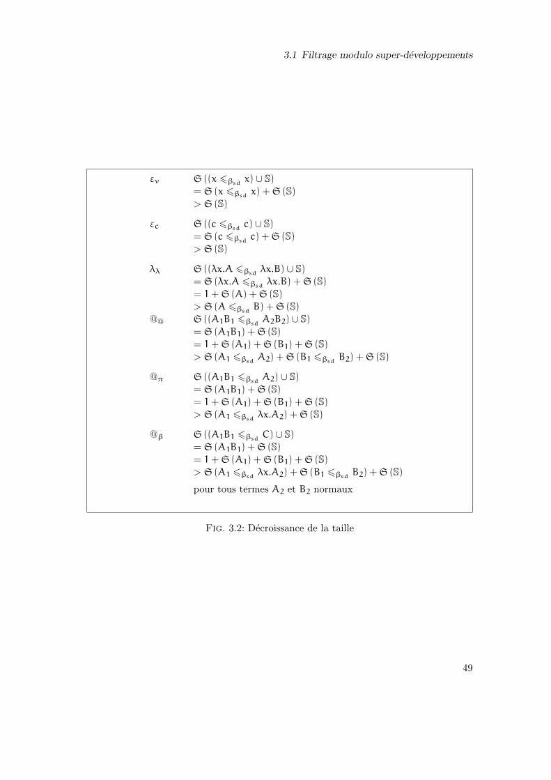
3.1 Filtrage modulo super-developpements
εv S((x 6βsdx) ∪ S)
= S (x 6βsdx) + S (S)
> S(S)
εc S((c 6βsdc) ∪ S)
= S (c 6βsdc) + S (S)
> S(S)
λλ S((λx.A 6βsdλx.B) ∪ S)
= S (λx.A 6βsdλx.B) + S (S)
= 1+ S (A) + S (S)
> S(A 6βsdB) + S (S)
@@ S((A1B1 6βsdA2B2) ∪ S)
= S (A1B1) + S (S)
= 1+ S (A1) + S (B1) + S (S)
> S(A1 6βsdA2) + S (B1 6βsd
B2) + S (S)
@π S((A1B1 6βsdA2) ∪ S)
= S (A1B1) + S (S)
= 1+ S (A1) + S (B1) + S (S)
> S(A1 6βsdλx.A2) + S (S)
@β S((A1B1 6βsdC) ∪ S)
= S (A1B1) + S (S)
= 1+ S (A1) + S (B1) + S (S)
> S(A1 6βsdλx.A2) + S (B1 6βsd
B2) + S (S)
pour tous termes A2 et B2 normaux
Fig. 3.2: Decroissance de la taille
49

Chapitre 3 Algorithmes de filtrage d’ordre superieur
∅ ∈ βf
(A1, B1) ∈ βf E ∈ βf
(A1, B1) ∪ E ∈ βf
(A ′1, B
′1) ∈ βf (A ′′
1 , B′′1) ∈ βf
(A1, B1) ∈ βf (A ′1, B
′1) ∪ (A ′′
1 , B′′1) ∪ E ∈ βf
(A1, B1) ∪ E ∈ βf
(A ′1, B
′1) ∈ βf
(A1, B1) ∈ βf (A ′1, B
′1) ∪ E ∈ βf
(A1, B1) ∪ E ∈ βf
Fig. 3.3: Extension de =⇒βfaux multi-ensembles
U ( ) S ( )
εv = >
εc = >
λλ > >
εX >
@@ > >
@π > >
@β > >
Notons que la regle (εX) fait toujours decroıtre le nombre de variables resolues gracea la condition d’application de la regle : X ∈ S.
Completude
Nous definissons une extension de la relation =⇒βfaux multi-ensembles. Nous notons
dans cette section (A1, B1) ∈ βf a la place de A1 =⇒βfB1.
Definition 3.9 (Extension de =⇒βfaux multi-ensembles) Nous notons ∅ le multi-
ensemble vide. Nous definissons la relation sur les multi-ensembles par les regles d’infe-rence (nous surchargeons la notation utilisee pour la relation du meme nom definie surles termes) definies dans la Figure 3.3.
Propriete 3.10 (Completude) Pour tout systeme S, si φ ∈ M(S) alors il existe unesuite de transformations
S = S0→ S1→ . . .→ Sn
50

3.1 Filtrage modulo super-developpements
ou Sn est en forme resolue et σSn≤ φ.
Preuve. Nous supposons donne un systeme S0 tel que φ ∈ M(S0). On veut montrer qu’ilexiste une derivation tel que
S = S0→ S1→ . . .→ Sn
ou Sn est en forme resolue et σSn≤ φ.
Posons S0 = (A1 6βsdB1) ∪ . . . (Ap 6βsd
Bp). Soit E0 le multi-ensemble defini par
E0 = (A1φ,B1) ∪ . . . ∪ (Apφ,Bp)
Dire que φ ∈ M(S0) est equivalent a dire que E0 ∈ βf. Nous montrons la proposition parinduction sur la preuve de E0 ∈ βf.
1. Si E0 = ∅ alors S0 = ∅ et σS0est la substitution identite id. Le resultat est immediat
puisque pour toute substitution φ on a, id 6 φ.
2. Si E0 = (A1φ,B1) ∪ E ∈ βf avec (A1φ,B1) ∈ βf est prouvable sans aucune hypo-these et E ∈ βf. Par hypothese d’induction il existe une derivation (D)
S′0 = (A2 6βsd
B2) ∪ . . . ∪ (Ap 6βsdBp)
→ . . .
→ S′n
telle que σS ′n
6 φ. Ainsi si X ∈ Dom(σ ′n) alors Xσ ′
n = B1.
Supposons tout d’abord que A1 soit une constante ou une variable. Alors la deri-vation
S0 →εcεv
(A2 6βsdB2) ∪ . . . ∪ (Ap 6βsd
Bp)
→ . . .
→ S′n
est la derivation recherchee.
Supposons maintenant que A1 soit une variable de filtrage alors s’il n’existe pasd’etape de reduction de (D) ou X est instanciee (application de la regle (εX) a lavariable X) alors la derivation
(X 6βsdB1) ∪ (A2 6βsd
B2) ∪ . . . ∪ (Ap 6βsdBp)
→ . . .
→ (X 6βsdB1) ∪ S
′n
est la derivation recherchee.
Sinon (c’est-a-dire s’il existe une etape de derivation i0 de D durant laquelle X estinstanciee) alors X est forcement instanciee par B1 et la derivation suivante est la
51

Chapitre 3 Algorithmes de filtrage d’ordre superieur
derivation recherchee :
(X 6βsdB1) ∪ (A2 6βsd
B2) ∪ . . . ∪ (Ap 6βsdBp)
→ . . .
→i0 (B1 6βsdB1) ∪ S
′i0+1
→→ S′i0+1
→ . . .
→ S′n
3. Si E0 = (A1φ,B1) ∪ E ∈ βf avec (A1φ,B1) ∈ βf est prouvable en utilisant deuxhypotheses. On raisonne par cas sur la derniere regle utilisee dans la preuve de(A1φ,B1) ∈ βf.
– Regle (Red− @) Alors on a E0 = (A11φA
21φ,B1B2) ∪ E ∈ βf avec
(A11φ,B
11) ∈ βf (A2
1φ,B21) ∈ βf
(A11φA
21φ,B
11B
21) ∈ βf
et(A1
1φ,B11) ∪ (A2
1φ,B21) ∪ E ∈ βf
Par hypothese d’induction, il existe une derivation telle que
(A11 6βsd
B11) ∪ (A2
1 6βsdB2
1) ∪ (A2 6βsdB2) ∪ . . . ∪ (Ap 6βsd
Bp)
→ . . .
→ Sn
avec σSn6 φ.
Si A1 = X alors on a aussi (puisqu’alors A11 = B1
1 et A21 = B2
1 et donc que lesdeux equations correspondantes sont V-closes et n’influencent pas la derivation)
(A2 6βsdB2) ∪ . . . ∪ (Ap 6βsd
Bp)
→ . . .
→ S′n
telle que σS ′n
6 φ. On conclut comme dans la cas precedent.Sinon, la derivation
(A1 6βsdB1) ∪ . . . ∪ (Ap 6βsd
Bp)
= (A11A
21 6βsd
B11B
21) ∪ (A2 6βsd
B2) ∪ . . . ∪ (Ap 6βsdBp)
→ (A11 6βsd
B11) ∪ (A2
1 6βsdB2
1) ∪ . . . ∪ (Ap 6βsdBp)
→ . . .
→ Sn
est la derivation recherchee.– Regle (Red− βf) Alors on a E0 = (A1
1φA21φ,B
11[x := B2
1]) ∪ E avec
(A11φ, λx.B
11) ∈ βf (A2
1φ,B21) ∈ βf
(A11φA
21φ,B
11[x := B2
1]) ∈ βf
52

3.1 Filtrage modulo super-developpements
et
(A11φ, λx.B
11) ∪ (A2
1φ,B21) ∪ E ∈ βf
Par hypothese d’induction, il existe une derivation telle que
(A11 6βsd
λx.B11) ∪ (A2
1 6βsdB2
1) ∪ . . . ∪ (Ap 6βsdBp)
→ . . .
→ S′n
avec σ ′Sn
6 φ. La derivation
(A11A
21 6βsd
B11[x := B2
1]) ∪ (A11 6βsd
λx.B11) ∪ (A2
1 6βsdB2
1) ∪ . . . ∪ (Ap 6βsdBp)
→ . . .
→ Sn
est la derivation recherchee si x ∈ fv(B11). Sinon, la derivation
(A11A
21 6βsd
B11[x := B2
1]) ∪ (A11 6βsd
λx.B11) ∪ . . . ∪ (Ap 6βsd
Bp)
→ . . .
→ Sn
est la derivation recherchee.
4. Ce cas est similaire au precedent.
Correction
Lemme 3.11 Pour tous systemes S et S′ tels que S → S
′ en utilisant les regles (εc),(εv), (λλ) ou (εX), on a M(S ′) = M(S).
Preuve. Le seul cas non trivial concerne la regle (εX). Soient X une variable de filtrage,S un systeme et A un terme tel que fv(A) = ∅ et X ∈ S.
φ ∈ M((X 6βsdA) ∪ S) ⇔ Xφ =⇒βf
A et φ ∈ M(S)φ normale⇔ Xφ = A et φ A/X ∈ M(S)
⇔ Xφ =⇒βfA et φ ∈ M(SA/X)
⇔ φ ∈ M((X 6βsdA) ∪ SA/X)
Lemme 3.12 Pour tous systemes S and S′ tels que S→ S
′ en utilisant les regles (@@),(@π) ou (@β) on a M(S ′) ⊆ M(S).
53
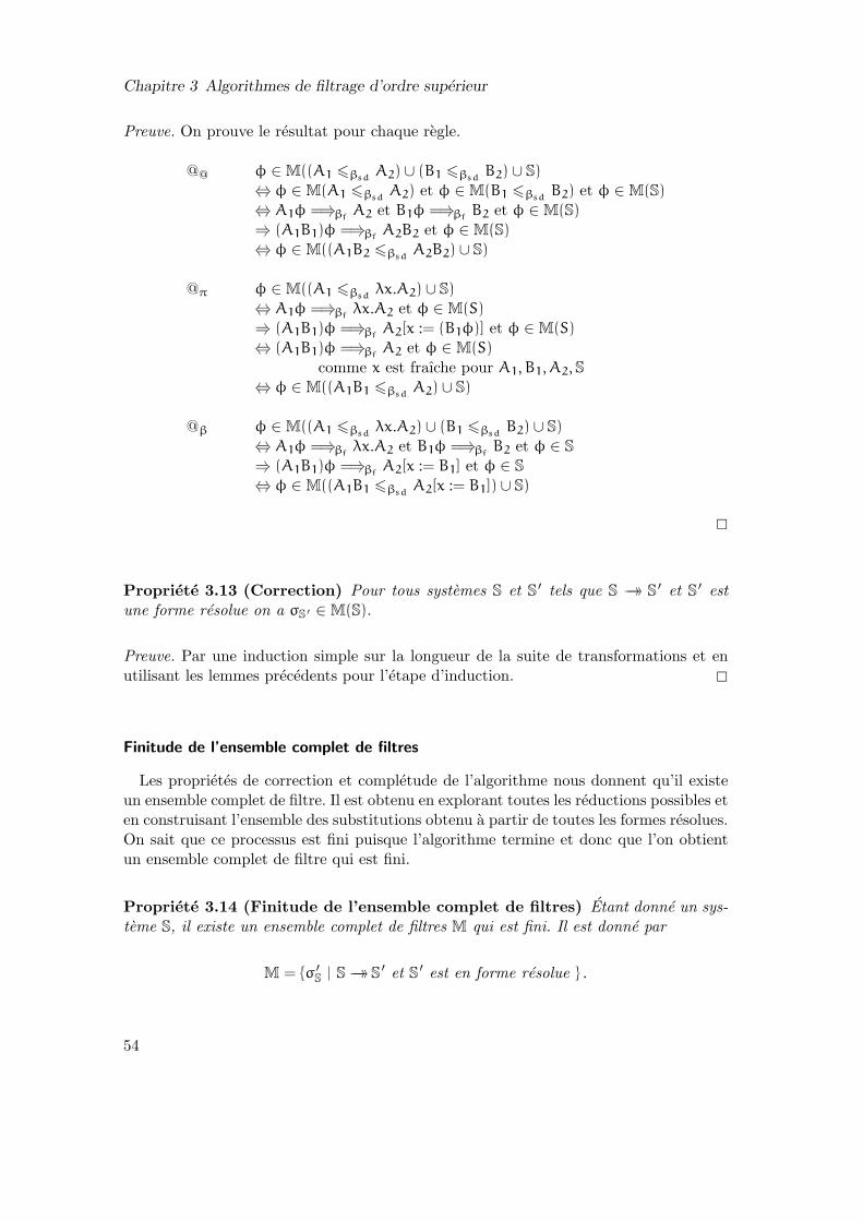
Chapitre 3 Algorithmes de filtrage d’ordre superieur
Preuve. On prouve le resultat pour chaque regle.
@@ φ ∈ M((A1 6βsdA2) ∪ (B1 6βsd
B2) ∪ S)
⇔ φ ∈ M(A1 6βsdA2) et φ ∈ M(B1 6βsd
B2) et φ ∈ M(S)
⇔ A1φ =⇒βfA2 et B1φ =⇒βf
B2 et φ ∈ M(S)
⇒ (A1B1)φ =⇒βfA2B2 et φ ∈ M(S)
⇔ φ ∈ M((A1B2 6βsdA2B2) ∪ S)
@π φ ∈ M((A1 6βsdλx.A2) ∪ S)
⇔ A1φ =⇒βfλx.A2 et φ ∈ M(S)
⇒ (A1B1)φ =⇒βfA2[x := (B1φ)] et φ ∈ M(S)
⇔ (A1B1)φ =⇒βfA2 et φ ∈ M(S)
comme x est fraıche pour A1, B1, A2,S
⇔ φ ∈ M((A1B1 6βsdA2) ∪ S)
@β φ ∈ M((A1 6βsdλx.A2) ∪ (B1 6βsd
B2) ∪ S)
⇔ A1φ =⇒βfλx.A2 et B1φ =⇒βf
B2 et φ ∈ S
⇒ (A1B1)φ =⇒βfA2[x := B1] et φ ∈ S
⇔ φ ∈ M((A1B1 6βsdA2[x := B1]) ∪ S)
Propriete 3.13 (Correction) Pour tous systemes S et S′ tels que S →→ S
′ et S′ est
une forme resolue on a σS ′ ∈ M(S).
Preuve. Par une induction simple sur la longueur de la suite de transformations et enutilisant les lemmes precedents pour l’etape d’induction.
Finitude de l’ensemble complet de filtres
Les proprietes de correction et completude de l’algorithme nous donnent qu’il existeun ensemble complet de filtre. Il est obtenu en explorant toutes les reductions possibles eten construisant l’ensemble des substitutions obtenu a partir de toutes les formes resolues.On sait que ce processus est fini puisque l’algorithme termine et donc que l’on obtientun ensemble complet de filtre qui est fini.
Propriete 3.14 (Finitude de l’ensemble complet de filtres) Etant donne un sys-teme S, il existe un ensemble complet de filtres M qui est fini. Il est donne par
M = σ ′S | S→→ S
′ et S′ est en forme resolue .
54

3.2 Filtrage modulo η et super-developpements
3.2 Filtrage modulo η et super-developpements
3.2.1 Regles
L’algorithme pour le filtrage modulo super-developpements donne dans la figure 3.1doit etre ajuste en deux points pour tenir compte de l’η-conversion. Tout d’abord, l’η-expansion est faite a la demande en ajoutant la regle suivante :
(λx.A 6βsdη B) ∪ S → (A 6βsdη Bx) ∪ S
si B n’est pas une λ-abstractionet x est une variable fraıche
Cette regle remplace le membre droit B par λx.Bx et effectue (comme dans la regle (λλ)de la figure 3.1) une elimination de la λ-abstraction en tete.
Ensuite, nous devons ajouter une condition a la regle (@β) de maniere a ce que λx.A2
et A1 soient en forme βη-normale (et non plus seulement en forme β-normale).
En effectuant ces deux changements on obtient ainsi un algorithme pour le filtragemodulo super-developpements et η. Nous le redonnons explicitement dans la figure 3.4mais en choisissant de ne pas eliminer les λ-abstractions mais plutot de les conserver enprefixe (et donc la regle (λλ) disparaıt).
On peut finalement remarquer que l’algorithme ainsi obtenu dispose des memes pro-prietes (terminaison, correction et completude). La preuve de terminaison ainsi que lapreuve de correction sont sans aucune difficulte. La preuve de completude est legerementplus technique mais fondamentalement identique a celle donnee dans la section 3.1.2.
Exemple 3.15 (βsdη-filtres) Considerons l’equation donnee dans l’exemple 3.1. Si onresout cette equation modulo βsdη on obtient seulement 4 solutions. En effet, les deuxsolutions
(X 6βsda) ∪ (Y 6βsd
b) et (X 6βsdλx.ax) ∪ (Y 6βsd
b)
sont η-equivalentes.
Exemple 3.16 (Solutions d’une βsdη-equation) Considerons le couple de termes(λx.X(Yx), a). Ce couple est une βsd-equation qui n’a pas de βsd-filtre solution.
Par contre, cette equation a deux βsdη-filtres donnes par
a/X, λz.z/Y et λz.z/X, a/Y.
55

Chapitre 3 Algorithmes de filtrage d’ordre superieur
(λxn.(A1B1) 6βsdλxn.(A2B2)) ∪ S →@@
(λxn.A1 6βsdλxn.A2)∪
(λxn.B1 6βsdλxn.B2) ∪ S
(λxn.(A1B1) 6βsdλxn.C) ∪ S →@π
(λxn.A1 6βsdλxn.(λy.C)) ∪ S
ou y variable fraıche
(λxn.(A1B1) 6βsdλxn.C) ∪ S →@β
(λxn.A1 6βsdλxn.(λx.A2))∪
(λxn.B1 6βsdλxn.B2) ∪ S
ou A2[x := B2] = C
et x variable fraıche, x ∈ fv(A2)
et λx.A2, B2 βη-normaux
(λxn.A 6βsdλxn−k.B) ∪ S →λ (λxn.A 6βsd
λxn−k+1.Bxn−k+1) ∪ S
(λxn.x 6βsdλxn.x) ∪ S →εv S
(λxn.a 6βsdλxn.a) ∪ S →εc S
(λxn.X 6βsdλxn.A) ∪ S →εX
(λxn.X 6βsdλxn.A) ∪ SA/X
si fv(A) = ∅ et X ∈ S
Fig. 3.4: Regles pour le filtrage modulo η et super-developpements
56

3.2 Filtrage modulo η et super-developpements
En effet,
(λx.(X(Yx) 6βsdη a) → (λx.X(Yx) 6βsdη λx.ax)
→ (λx.X 6βsdη λx.a) ∪ (λx.Yx 6βsdη λx.x)
→ (λx.X 6βsdη λx.a) ∪ (λx.Y 6βsdη λx.λz.z)
(λx.X(Yx) 6βsdη a) → (λx.X(Yx) 6βsdη λx.ax)
→ (λx.X 6βsdη λx.λz.z) ∪ (λx.Yx 6βsdη λx.ax)
→ (λx.X 6βsdη λx.λz.z) ∪ (λx.Y 6βsdη λx.a)
3.2.2 Minimalite pour les motifs a la Miller
Nous poursuivons la comparaison, commencee dans la section 2.2.4, entre le filtragemodulo super-developpements et le filtrage de motifs a la Miller. Dans la suite de cettesection, nous appellerons equation de motifs a la Miller une βsd-equation dont le premierterme est un motif a la Miller.
L’algorithme donne pour le filtrage modulo η et super-developpements applique a unmotif a la Miller donne au plus une solution (proposition suivante). Comme l’algorithmeest correct et complet, cette solution est le filtre le plus general.
On peut tout d’abord remarquer que tout reduit d’un systeme d’equations a la Millerest un systeme d’equations a la Miller.
Propriete 3.17 Soit P 6βsdη B une βsd-equation ou P est un motif a la Miller qui aune solution et A un terme type. Alors l’ensemble des formes resolues donnees par lesregles de la figure 3.4 est un singleton.
Preuve. Nous pouvons tout d’abord remarquer que si la regle (λ ) s’applique alors aucuneautre regle ne peut s’appliquer et donc cette situation n’introduit pas de choix dansl’application des regles. Nous l’exclurons donc dans le reste de la preuve.
Nous prouvons le resultat par induction sur la taille des motifs. On distingue trois cassuivant le symbole de tete du motif.
1. Si P = λxn.f(A1, . . . , An) alors, pour que l’equation est une solution alors neces-sairement B doit etre de la forme B = λxn.f(B1, . . . , Bp). Toutes les derivations quimenent a une solution doivent reduire P 6βsd
B en
(λxn.A1 6βsdλxn.B1) ∪ . . . ∪ (λxn.Ap 6βsd
λxn.Bp)
(modulo l’ordre d’application des regles).
57

Chapitre 3 Algorithmes de filtrage d’ordre superieur
Or λxn.A1, . . . λxn.Ap sont des motifs a la Miller donc on peut appliquer l’hypo-these d’induction et conclure que
λxn.A1 6βsdλxn.B1 a pour unique solution σ1
. . .
λxn.Ap 6βsdλxn.Bp a pour unique solution σp
donc le probleme initial a pour unique solution σ1 ∪ . . . ∪ σp.
2. Le cas P = λxn.x(A1, . . . , An) est similaire au precedent.
3. Si P = λxn.X(xi1 , . . . , xip ) ou les variables xi1 , . . . , xip sont deux a deux differentes.Alors trois regles peuvent s’appliquer (@π), (@@) ou (@β). Nous allons montrer quedans tous les cas un seul de ces choix mene a une solution.
Dans la suite de cette preuve, nous utiliserons constamment le fait que si l’appli-cation de la regle (@@) mene a une solution alors necessairement B = B1xip . Dememe si l’application de la regle (@β) mene a une solution alors
(λxn.X(xi1 , . . . , xip ) 6βsdλxn.B) → (λxn.X(xi1 , . . . , xip−1
) 6βsdλxn.λz.C1∪)
(λxn.xip 6βsdλxn.xip )
avec B = C1[z := xip ] et z ∈ fv(C1)
et donc xip ∈ fv(B).
Supposons tout d’abord que l’application de la regle (@π) mene a une solution.Montrons alors que ni l’application de la regle (@@) ni l’application de la regle(@β) aboutissent a une solution. On a
(λxn.X(xi1 , . . . , xip ) 6βsdλxn.B)
→ (λxn.X(xi1 , . . . , xip−1) 6βsd
λxn.λy.B)
Forcement, le terme B ne contient pas la variable xip (car aucune des variablesxi1 , . . . , xip−1
n’est egale a xip ). Le resultat est donc immediat.
Supposons maintenant que l’application de la regle (@@) mene a une solution.Montrons alors que ni l’application de la regle (@π) ni l’application de la regle(@β) aboutissent une solution. On a
(λxn.X(xi1 , . . . , xip ) 6βsdλxn.B1xip )
→ (λxn.X(xi1 , . . . , xip−1) 6βsd
λxn.B1) ∪ (λxn.xip 6βsdλxn.xip
De la deuxieme equation, on deduit que xip ∈ fv(B) et donc (voir ci-dessus) quela regle (@π) ne mene pas a une solution. De la premiere equation on deduit quexip 6∈ fv(B1).
Essayons d’appliquer la regle (@β). On cherche C1 tel que B1xn = C1[z := xn].Mais comme xip 6∈ fv(B1), necessairement C1 = B1z avec z 6∈ fv(B1) mais leterme λz.B1z n’est pas βη-normal donc la regle ne s’applique pas. Ce qui conclutla preuve.
58

3.3 Filtrage du second ordre
3.3 Filtrage du second ordre
Dans cette section, nous considerons le filtrage d’ordre deux modulo βη. Nous allonsmontrer que l’algorithme pour le filtrage modulo les super-developpements applique dansun cadre type donne un algorithme pour le filtrage d’ordre deux. Ceci repose sur lesproprietes de l’algorithme de filtrage modulo les super-developpements que nous etudionsdans la section 3.3.2. Nous rappelons tout d’abord l’algorithme de filtrage du second-ordre propose dans [HL78]. Un algorithme plus efficace a ete propose dans [CQS96].
3.3.1 Algorithme de Huet et Lang
Nous rappelons dans cette section l’algorithme pour le filtrage du second ordre mo-dulo βη donne dans [HL78]. Cet algorithme est une particularisation de l’algorithmed’unification propose dans [Hue76] et presente sous forme de regles de transformationsdans [SG89]. Nous adaptons cette derniere presentation au cas du second ordre commecela a ete fait dans [CQS96]. Rappelons que nous ne considerons pour cet algorithmeque tous les termes sont en forme normale β-longue. L’application de substitutions esten particulier normalisante.
Les regles de transformation de l’algorithme de la figure 3.5 transforment un coupleforme d’un multi-ensemble d’equations de filtrage et d’une substitution. Etant donne uncouple 〈S, id〉 l’algorithme reussit s’il existe une suite de transformations terminant sur〈∅, σ〉. La substitution σ est dans ce cas (correction de l’algorithme) un filtre pour S.
La premiere regle (Decomposition) simplifie une equation dont les symboles de tetesont identiques. Les regles (Projection) et (Imitation) traitent le cas des equations dont latete du membre gauche est une variable de filtrage. Dans le premier cas, la variable estinstanciee par une fonction de projection. C’est donc l’argument projete qu’il va falloirrendre egal au membre droit. Dans le second cas, on realise une instanciation partielle dela variable de filtrage dans le sens suivant : le symbole de tete du terme associe a cettevariable est fixe a partir de celui du membre droit ; on introduit de nouvelles variablesde filtrage pour effectuer les choix restants1.
Nous aurions pu presenter les algorithmes donnes precedemment en construisant l’even-tuelle substitution solution au fur et a mesure. Nous ne l’avons pas fait pour alleger lapresentation des regles de transformation (alors que dans le cas present c’est indispen-sable).
Nous illustrons l’algorithme donne dans la figure 3.5 sur un exemple.
Exemple 3.18 Considerons l’equation (λx.X(x, a) 6βη λx.f(a, x, a)) ou a et f sontdes constantes de types appropries. Clairement, la regle (Decomposition) ne peut pass’appliquer. Appliquer la regle (Projection) mene a un blocage puisque les deux argumentsde X (qui sont x et a) ne sont pas filtrables avec le membre droit. Par contre, la regle
1L’instanciation partielle implique notamment que l’on peut substituer des variables de filtrage par des
termes non V-clos. Nous sortons donc temporairement dans cette section du cadre defini jusqu’ici
afin d’exprimer l’algorithme de Huet et Lang dans sa presentation standard.
59
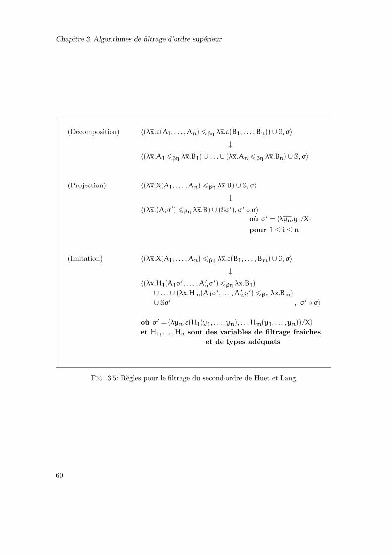
Chapitre 3 Algorithmes de filtrage d’ordre superieur
(Decomposition) 〈(λx.ε(A1, . . . , An) 6βη λx.ε(B1, . . . , Bn)) ∪ S, σ〉
↓〈(λx.A1 6βη λx.B1) ∪ . . . ∪ (λx.An 6βη λx.Bn) ∪ S, σ〉
(Projection) 〈(λx.X(A1, . . . , An) 6βη λx.B) ∪ S, σ〉
↓〈(λx.(Aiσ
′) 6βη λx.B) ∪ (Sσ ′), σ ′ σ〉ou σ ′ = λyn.yi/X
pour 1 ≤ i ≤ n
(Imitation) 〈(λx.X(A1, . . . , An) 6βη λx.ε(B1, . . . , Bm) ∪ S, σ〉
↓〈(λx.H1(A1σ
′, . . . , A ′nσ
′) 6βη λx.B1)
∪ . . . ∪ (λx.Hm(A1σ′, . . . , A ′
nσ′) 6βη λx.Bm)
∪ Sσ ′ , σ ′ σ〉
ou σ ′ = λyn.ε(H1(y1, . . . , yn), . . . Hm(y1, . . . , yn))/X
et H1, . . . , Hn sont des variables de filtrage fraıches
et de types adequats
Fig. 3.5: Regles pour le filtrage du second-ordre de Huet et Lang
60

3.3 Filtrage du second ordre
(Imitation) s’applique et donne
〈(λx.H1(x, a) 6βη λx.a)
∪ (λx.H2(x, a) 6βη λx.x) , λy1y2.f(H(y1, y2), H2(y1, y2), H3(y1, y2)/X〉∪ (λx.H3(x, a) 6βη λx.a)
La resolution des equations faisant intervenir H1, H2 et H3 donnent pour chacune deces trois equations les solutions suivantes
λz1z2.a/H1 ou λz1z2.z2/H1
λz1z2.z1/H2
λz1z2.a/H3 ou λz1z2.z2/H3
Il existe donc quatre solutions a l’equation initiale qui sont donnees par
λy1y2.f(a, y1, a)/X
λy1y2.f(a, y1, y2)/X
λy1y2.f(y2, y1, a)/X
λy1y2.f(y2, y1, y2)/X
3.3.2 Filtrage modulo super-developpements et types
Nous pouvons tout d’abord remarquer que si un systeme est constitue uniquement determes bien types alors tous ses reduits sont constitues de termes bien types. L’algorithmedonne dans la figure 3.1 se comporte bien vis a vis des types dans le sens suivant : unesuite de transformations qui aboutit a un systeme bien type (c’est-a-dire un systeme telque les deux membres de chacune des equations sont des termes bien types et de memetype) ne peut pas mettre en œuvre de systemes mal types.
Propriete 3.19 Pour tous systemes S et S′ tels que S →→ S
′, si le systeme S′ est bien
type alors le systeme S est aussi bien type.
Cette proposition est une consequence directe du lemme suivant :
Lemme 3.20 Pour tout systeme S tel que S ne soit pas bien type et tout systeme S′ tel
que S→ S′, le systeme S
′ n’est pas bien type.
Preuve. Supposons donne un systeme S qui ne soit pas bien type. On montre que tousles reduits de S ne sont pas bien types en analysant regle par regle
– Regles (εv) et (εc) : immediat.– Regle (εX) : Les systemes S et S
′ sont respectivement definis par S = (X 6βsdA)∪S0
et parS′ = (X 6βsd
A) ∪ S0A/X. Si l’equation (X 6βsdA) n’est pas bien typee alors
le resultat est immediat. Sinon (si X 6βsdA est bien typee c’est-a-dire si X et A
sont deux termes bien types de meme type) le systeme S0 n’est pas bien type. Maiscomme X et A sont de meme type, alors S0A/X n’est donc pas bien type.
61
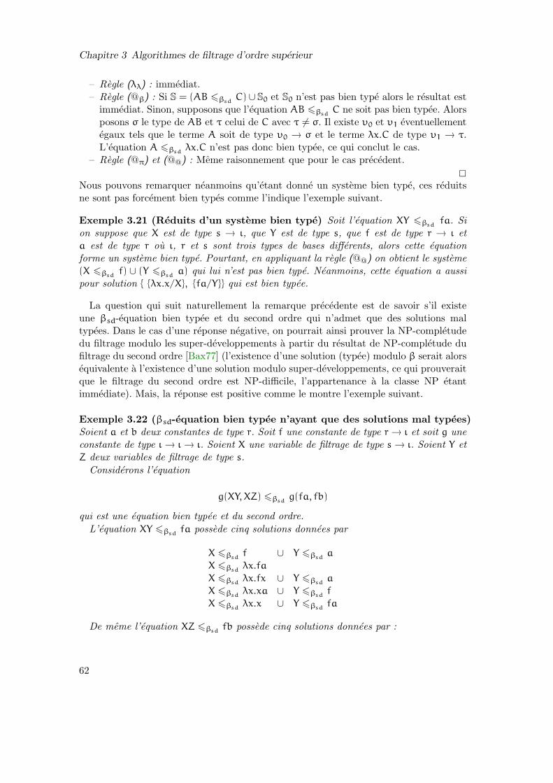
Chapitre 3 Algorithmes de filtrage d’ordre superieur
– Regle (λλ) : immediat.– Regle (@β) : Si S = (AB 6βsd
C)∪ S0 et S0 n’est pas bien type alors le resultat estimmediat. Sinon, supposons que l’equation AB 6βsd
C ne soit pas bien typee. Alorsposons σ le type de AB et τ celui de C avec τ 6= σ. Il existe υ0 et υ1 eventuellementegaux tels que le terme A soit de type υ0 → σ et le terme λx.C de type υ1 → τ.L’equation A 6βsd
λx.C n’est pas donc bien typee, ce qui conclut le cas.– Regle (@π) et (@@) : Meme raisonnement que pour le cas precedent.
Nous pouvons remarquer neanmoins qu’etant donne un systeme bien type, ces reduitsne sont pas forcement bien types comme l’indique l’exemple suivant.
Exemple 3.21 (Reduits d’un systeme bien type) Soit l’equation XY 6βsdfa. Si
on suppose que X est de type s → ι, que Y est de type s, que f est de type r → ι eta est de type r ou ι, r et s sont trois types de bases differents, alors cette equationforme un systeme bien type. Pourtant, en appliquant la regle (@@) on obtient le systeme(X 6βsd
f) ∪ (Y 6βsda) qui lui n’est pas bien type. Neanmoins, cette equation a aussi
pour solution λx.x/X, fa/Y qui est bien typee.
La question qui suit naturellement la remarque precedente est de savoir s’il existeune βsd-equation bien typee et du second ordre qui n’admet que des solutions maltypees. Dans le cas d’une reponse negative, on pourrait ainsi prouver la NP-completudedu filtrage modulo les super-developpements a partir du resultat de NP-completude dufiltrage du second ordre [Bax77] (l’existence d’une solution (typee) modulo β serait alorsequivalente a l’existence d’une solution modulo super-developpements, ce qui prouveraitque le filtrage du second ordre est NP-difficile, l’appartenance a la classe NP etantimmediate). Mais, la reponse est positive comme le montre l’exemple suivant.
Exemple 3.22 (βsd-equation bien typee n’ayant que des solutions mal typees)Soient a et b deux constantes de type r. Soit f une constante de type r→ ι et soit g uneconstante de type ι→ ι→ ι. Soient X une variable de filtrage de type s→ ι. Soient Y etZ deux variables de filtrage de type s.
Considerons l’equation
g(XY,XZ) 6βsdg(fa, fb)
qui est une equation bien typee et du second ordre.
L’equation XY 6βsdfa possede cinq solutions donnees par
X 6βsdf ∪ Y 6βsd
a
X 6βsdλx.fa
X 6βsdλx.fx ∪ Y 6βsd
a
X 6βsdλx.xa ∪ Y 6βsd
f
X 6βsdλx.x ∪ Y 6βsd
fa
De meme l’equation XZ 6βsdfb possede cinq solutions donnees par :
62
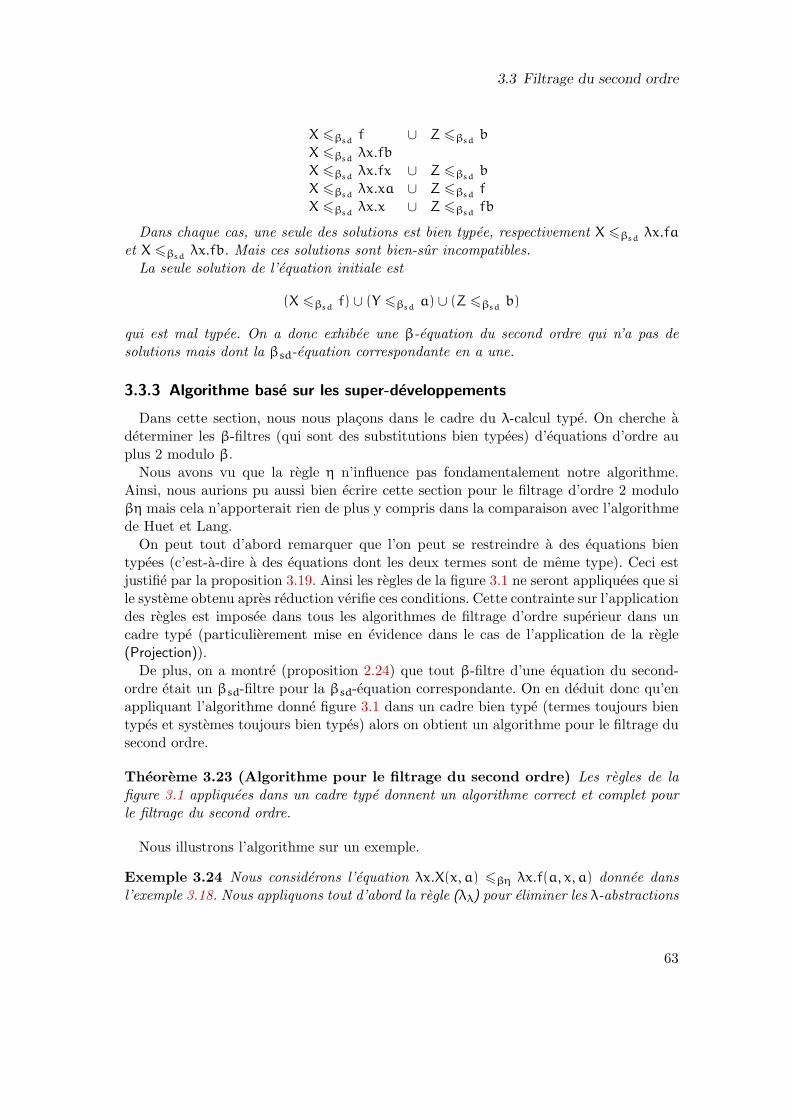
3.3 Filtrage du second ordre
X 6βsdf ∪ Z 6βsd
b
X 6βsdλx.fb
X 6βsdλx.fx ∪ Z 6βsd
b
X 6βsdλx.xa ∪ Z 6βsd
f
X 6βsdλx.x ∪ Z 6βsd
fb
Dans chaque cas, une seule des solutions est bien typee, respectivement X 6βsdλx.fa
et X 6βsdλx.fb. Mais ces solutions sont bien-sur incompatibles.
La seule solution de l’equation initiale est
(X 6βsdf) ∪ (Y 6βsd
a) ∪ (Z 6βsdb)
qui est mal typee. On a donc exhibee une β-equation du second ordre qui n’a pas desolutions mais dont la βsd-equation correspondante en a une.
3.3.3 Algorithme base sur les super-developpements
Dans cette section, nous nous placons dans le cadre du λ-calcul type. On cherche adeterminer les β-filtres (qui sont des substitutions bien typees) d’equations d’ordre auplus 2 modulo β.
Nous avons vu que la regle η n’influence pas fondamentalement notre algorithme.Ainsi, nous aurions pu aussi bien ecrire cette section pour le filtrage d’ordre 2 moduloβη mais cela n’apporterait rien de plus y compris dans la comparaison avec l’algorithmede Huet et Lang.
On peut tout d’abord remarquer que l’on peut se restreindre a des equations bientypees (c’est-a-dire a des equations dont les deux termes sont de meme type). Ceci estjustifie par la proposition 3.19. Ainsi les regles de la figure 3.1 ne seront appliquees que sile systeme obtenu apres reduction verifie ces conditions. Cette contrainte sur l’applicationdes regles est imposee dans tous les algorithmes de filtrage d’ordre superieur dans uncadre type (particulierement mise en evidence dans le cas de l’application de la regle(Projection)).
De plus, on a montre (proposition 2.24) que tout β-filtre d’une equation du second-ordre etait un βsd-filtre pour la βsd-equation correspondante. On en deduit donc qu’enappliquant l’algorithme donne figure 3.1 dans un cadre bien type (termes toujours bientypes et systemes toujours bien types) alors on obtient un algorithme pour le filtrage dusecond ordre.
Theoreme 3.23 (Algorithme pour le filtrage du second ordre) Les regles de lafigure 3.1 appliquees dans un cadre type donnent un algorithme correct et complet pourle filtrage du second ordre.
Nous illustrons l’algorithme sur un exemple.
Exemple 3.24 Nous considerons l’equation λx.X(x, a) 6βη λx.f(a, x, a) donnee dansl’exemple 3.18. Nous appliquons tout d’abord la regle (λλ) pour eliminer les λ-abstractions
63

Chapitre 3 Algorithmes de filtrage d’ordre superieur
de tete. Examinons ensuite quelles sont les possibilites d’application de la regle (@β),autrement dit quelles sont les instanciations de B1 et B2 (en suivant les notations de lafigure 3.1). Puisque l’on doit avoir a 6βsd
B2, necessairement B2 = a. Il y a donc troischoix pour B1 :
1. B1 = λy2.f(y2, x, y2) ;
2. B1 = λy2.f(y2, x, a) ;
3. B1 = λy2.f(a, x, y2).
Chacun de ses choix conduit aux solutions
λy1y2.f(y2, y1, y2)/X
λy1y2.f(y2, y1, a)/X
λy1y2.f(a, y1, y2)/X
De plus, en appliquant la regle (@π) on retrouve la quatrieme solution a savoir
λy1y2.f(a, y1, a)/X.
Remarque 3.25 (Comparaisons des algorithmes pour le filtrage du 2nd ordre)Les algorithmes pour lne filtrage d’ordre 2 de Huet et Lang et celui base sur les super-developpements sont relativement differents. En pensant a une representation des termessous forme d’arbre, l’algorithme de Huet et Lang compare les termes par le bas (symbolede tete) alors que l’algorithme base sur les super-developpements compare les termes parle haut (comparaison des arguments, voir remarque 3.3).
Conclusion
Nous avons vu que le filtrage modulo super-developpements est un outil simple maispuissant qui a l’avantage de ne pas etre lie a un systeme de type. Nous verrons dans lechapitre suivant, apres avoir introduit les definitions necessaires, que cette approche estparticulierement prometteuse pour l’etude du filtrage d’ordre superieur dans les calculsavec motifs et plus particulierement le ρ-calcul.
D’autre part, la comprehension que nous avons apportee du filtrage modulo super-developpements permet un regard nouveau sur le travail d’explicitation [BCK06] dufiltrage dans les CRS. Il nous apparaıt maintenant claire que ce filtrage est le filtragemodulo developpements, ce qui n’est pas surprenant a posteriori puisque le meta-langagedes CRS est le λ-calcul avec developpements.
En mettant en avant les proprietes du λ-calcul avec super-developpements et plusparticulierement celles du filtrage associe, nous soulignons que le λ-calcul avec super-developpements est un meta-langage (ou « substitution calculus » au sens de van Raam-donk et van Oostrom) bien adapte a la reecriture d’ordre superieur. On definit ainsi unnouveau formalisme d’ordre superieur qu’il convient d’appeler les super-CRS.
64

Part II
Structures of the rewriting calculus
65


Chapter 4
The rewriting calculus
Context We present here the background theory that originally lead to the differentworks presented in this thesis. The rewriting calculus, also called the ρ-calculus, wasintroduced to give a semantics to rewrite-based languages such as Elan and in particularto rewriting strategies [BKK98a, BKK96]. To have a control on the rewriting relation,the ρ-calculus makes all the ingredients of rewriting explicit objects, in particular thenotion of rule, application and result.
The ρ-calculus is a higher-order formalism that inherits from the λ-calculus its higher-order capabilities: the explicit treatment of functions and their applications. To expressrewrite rules, the λ-abstraction is generalized to an abstraction on patterns. This meansthat the evaluation is based on pattern-matching that can be performed syntactically ormodulo an equational theory. In the latter case, it may give several results that are allrepresented, in the ρ-calculus, with term collections, allowing a natural handling of thenon-determinism of rewriting.
The first version of the ρ-calculus appears in [CK01, Cir00, CK98a] and focusses onthe encoding of rewriting and rewriting strategies. A simplified version [CKL01] focuseson the encoding of λ-calculi of objects. Several extensions of the plain ρ-calculus havebeen proposed in order to handle different problems: to deal with exceptions [FK02],to handle explicitly matching and substitutions (Chapter 5), to deal with imperativefeatures [LS04], to handle term-graphs instead of terms [BBCK04, Ber05] etc.
A polymorphic type system can be found in [CKL02] and type checking and type in-ference issues have been studied in [LW04]. The approach is extended to Pure PatternsType Systems [BCKL03], a generalization of Pure Type Systems for the ρ-calculus. Ithas been shown that the simply-typed pure pattern type system ensures strong nor-malization [Wac05]. The ρ-calculus is useful in logic, more particularly in relation withdeduction modulo [Wac05].
The ρ-calculus is in fine an extension of the λ-calculus with pattern-matching andterm-collections. The combination of the λ-calculus with first-order term rewriting hasbeen already handled by enriching first-order rewriting with higher-order capabilities,like for example in the Combinatory Reduction Systems (CRS) [Klo80, KOR93]. Thelink between the two formalisms has already been studied for the simplest version of theρ-calculus (first-order algebraic patterns and term collections as tuples). In fact, CRS canbe encoded in the ρ-calculus [BCK06, Ber05] and conversely, the simplest version of the ρ-calculus can also be encoded by an orthogonal CRS [BK07]. As a consequence, importantproperties like confluence, finite developments and standardisation are deduced for the
67

Chapter 4 The rewriting calculus
corresponding version of the rewriting calculus.
Contributions In this chapter, we summarize basic definitions and properties of someρ-calculi. In the following chapter, we will extend the basic ρ-calculus to deal explicitlywith the matching and the application of substitutions. The different extensions of theρ-calculus will be used to give instances of the general calculus defined in Chapter 6.
Following the work presented in Part I on higher-order matching in the λ-calculus, wegive some hints on higher-order matching in the ρ-calculus.
Outline of the chapter In Section 4.1 and Section 4.2 we introduce the syntax andthe operational semantics of the ρ-calculus. In Section 4.3 we give some already knownresults on the confluence of the ρ-calculus. In Section 4.4, we give some results onthe expressiveness of the ρ-calculus. In Section 4.5, we present two extensions of theρ-calculus. Section 4.6 discusses higher-order matching in the ρ-calculus.
4.1 Syntax
Given a set of constants (denoted c, d, e, f, . . .) anda set of variables denoted x, y, z, . . .)and the set of ρ-terms is defined in Figure 4.1.
In the ρ-calculus, the usual λ-abstraction λx.A is generalized by a pattern-abstraction(also called rule abstraction) P _ A where P can be a more general pattern than a singlevariable x. The left-hand side of an abstraction defines the variables we abstract on andsome context information. An application is implicitly denoted by concatenation. Theterms can be grouped together into structures that can be seen as collections of terms.In an abstraction of the form P _ A we call the term P the pattern and the term A thebody.
We assume that the application operator associates to the left, while the other oper-ators associate to the right. The priority of the application operator is higher than thatof _ which is, in turn, of higher priority than the ≀ .
Definition 4.1 (Algebraic terms) We call algebraic the terms of the form
(. . . ((f A1)A2) . . .)An
where f is a constant. We usually denote them by f(A1, A2, . . . , An).
Definition 4.2 (Free and bound variables) The set of free variables of a term A
and the set of bound variables, denoted fv(A) and bv(A), are defined inductively by:
fv(c) , ∅ fv(x) , x
bv(c) , ∅ bv(x) , ∅
fv(AB) , fv(A ≀ B) , fv(A) ∪ fv(B) fv(P _ A) , fv(A)\fv(P)
bv(AB) , fv(A ≀ B) , bv(A) ∪ bv(B) bv(P _ A) , bv(A) ∪ bv(P) ∪ fv(P)
68
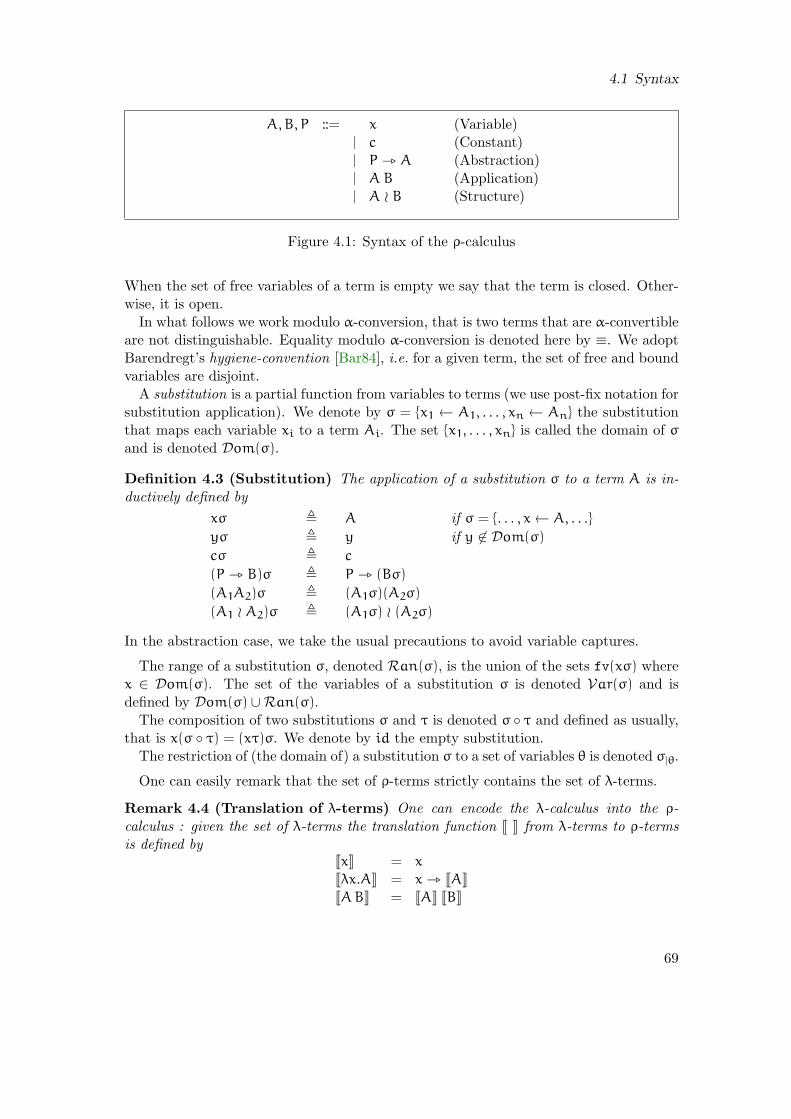
4.1 Syntax
A,B, P ::= x (Variable)| c (Constant)| P _ A (Abstraction)| A B (Application)| A ≀ B (Structure)
Figure 4.1: Syntax of the ρ-calculus
When the set of free variables of a term is empty we say that the term is closed. Other-wise, it is open.
In what follows we work modulo α-conversion, that is two terms that are α-convertibleare not distinguishable. Equality modulo α-conversion is denoted here by ≡. We adoptBarendregt’s hygiene-convention [Bar84], i.e. for a given term, the set of free and boundvariables are disjoint.
A substitution is a partial function from variables to terms (we use post-fix notation forsubstitution application). We denote by σ = x1 ← A1, . . . , xn ← An the substitutionthat maps each variable xi to a term Ai. The set x1, . . . , xn is called the domain of σand is denoted Dom(σ).
Definition 4.3 (Substitution) The application of a substitution σ to a term A is in-ductively defined by
xσ , A if σ = . . . , x← A, . . .
yσ , y if y 6∈ Dom(σ)
cσ , c
(P _ B)σ , P _ (Bσ)
(A1A2)σ , (A1σ)(A2σ)
(A1 ≀ A2)σ , (A1σ) ≀ (A2σ)
In the abstraction case, we take the usual precautions to avoid variable captures.
The range of a substitution σ, denoted Ran(σ), is the union of the sets fv(xσ) wherex ∈ Dom(σ). The set of the variables of a substitution σ is denoted Var(σ) and isdefined by Dom(σ) ∪Ran(σ).
The composition of two substitutions σ and τ is denoted σ τ and defined as usually,that is x(σ τ) = (xτ)σ. We denote by id the empty substitution.
The restriction of (the domain of) a substitution σ to a set of variables θ is denoted σ|θ.
One can easily remark that the set of ρ-terms strictly contains the set of λ-terms.
Remark 4.4 (Translation of λ-terms) One can encode the λ-calculus into the ρ-calculus : given the set of λ-terms the translation function J K from λ-terms to ρ-termsis defined by
JxK = x
Jλx.AK = x _ JAKJABK = JAK JBK
69

Chapter 4 The rewriting calculus
Thus, when translating λ-terms into ρ-terms the binder λ is replaced by the (rule) ab-straction operator _ like for the following terms:
λ-calculus ρ-calculus
λx.x x _ x
λx.λy.x x _ y _ x
λx.(x x) x _ x x
As we will see in the next section, this translation is consistent with the reduction in thetwo formalisms: for each β-reduction of a λ-term there exists a corresponding reductionof the translated term in the ρ-calculus.
Example 4.5 (Encoding of propositional formulae) Using the constants t, f, not,and, or, xor (denoting respectively the boolean values true and false, the negation, theconjunctionn the disjunction and the exclusive disjunction) we can define the followingpropositional formulae: and(x, t) and or(not(x), not(y)).
Example 4.6 (Rewrite rules) Some rules to compute in the Boolean algebra:
• and(x, t) _ x; the occurence of the variable x in the body is bound by the patternand(x, t).
in this abstraction the variable x in the body is bound by the variable in the pattern.
• not(and(x, y)) _ or(not(x), not(y)); this rule bounds the variables x and y.
• xor(x, x) _ f; a non-linear rule.
The application of the second rewrite rule to the term not(and(t, f)) is represented by theterm
(
not(and(x, y)) _ or(not(x), not(y)))
not(and(t, f))
and, as we will see in the next section, this term reduces to or(not(t), not(f)).
4.2 Operational semantics
The evaluation mechanism of the ρ-calculus relies of the fundamental operation of match-ing. When applying a pattern-abstraction, this operation allows to bind variables to theircorresponding values. The general framework of the ρ-calculus allows pattern-matchingto be performed syntactically or modulo an equational theory. The set of patterns andthe congruence on terms modulo which the matching is performed are thus parameters ofthe calculus. The third parameter is the underlying theory for the ≀ operator (typically,a combination of associativity, commutativity and idempotence). We will see that incase of non-unitary matching the third parameter can not be arbitrarily chosen.
In this section, we give some examples of matching algorithms that can be used in theevaluation of the ρ-calculus. We then define the operational semantics of the ρ-calculus.
70

4.2 Operational semantics
4.2.1 Matching
We first define the operation of matching and then give some examples of matchingalgorithms for different sets of patterns.
Definition 4.7 (Matching) Given a theory T, i.e. a set of axioms defining a congru-
ence relationT=, we define
1. A matching equation (also called a matching problem) is a pair denoted P ≺≺T A
with P a pattern and A a term.
2. A substitution σ is a solution of the matching equation P ≺≺T A if PσT= A.
The set of solutions of P ≺≺T A is denoted by Sol(P ≺≺T A).
We often consider Sol as a function that given a pattern and a term returns the setof substitutions (possibly empty) of the matching problem. When it is clear from thecontext, we do not always explicitly mention the congruence used to performed matching.
As we will see in the next sections, when studying confluent instances of the ρ-calculus,we consider particular sets of patterns.
Definition 4.8 ((Structure) algebraic patterns) The set of algebraic and structurealgebraic patterns are defined as follows:
Algebraic patterns P,Q ::= x
| c
| f(P1, P2, . . . , Pn)
Structure algebraic patterns P,Q ::= x
| c
| f(P1, P2, . . . , Pn)
| P ≀ Q
Definition 4.9 (Syntactic matching) We consider that the matching constraints areof the form A≪∅ B and we consider possibly empty conjunctions of such problems builtwith the associative commutative operator ∧ . The following set of terminating andconfluent rules can be used to solve the (non-linear) syntactic matching:
A≪∅ A ∧ M → M
(A1A2 ≪∅ B1B2) ∧ M → (A1 ≪∅ B1) ∧ (A2 ≪∅ B2) ∧ M
The set of solutions of a matching problem P ≺≺∅ A is obtained by normalizing thematching constraint P ≪∅ A w.r.t. the above rewrite rules and according to the obtainedresult we have:
71
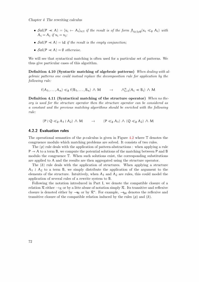
Chapter 4 The rewriting calculus
• Sol(P ≺≺ A) = xi ← Aii∈I if the result is of the form∧
i∈I6=∅(xi ≪∅ Ai) withAi = Aj if xi = xj;
• Sol(P ≺≺ A) = id if the result is the empty conjunction;
• Sol(P ≺≺ A) = ∅ otherwise.
We will see that syntactical matching is often used for a particular set of patterns. Wethus give particular cases of this algorithm.
Definition 4.10 (Syntactic matching of algebraic patterns) When dealing with al-gebraic patterns one could instead replace the decomposition rule for application by thefollowing rule:
f(A1, . . . , An) ≪∅ f(B1, . . . , Bn) ∧ M → ∧ni=1(Ai ≺≺ Bi) ∧ M
Definition 4.11 (Syntactical matching of the structure operator) When no the-ory is used for the structure operator then the structure operator can be considered asa constant and the previous matching algorithms should be enriched with the followingrule:
(P ≀ Q≪∅ A1 ≀ A2) ∧ M → (P ≪∅ A1) ∧ (Q≪∅ A2) ∧ M
4.2.2 Evaluation rules
The operational semantics of the ρ-calculus is given in Figure 4.2 where T denotes thecongruence modulo which matching problems are solved. It consists of two rules.
The (ρ) rule deals with the application of pattern-abstractions : when applying a ruleP _ A to a term B, we compute the potential solutions of the matching between P and Bmodulo the congruence T. When such solutions exist, the corresponding substitutionsare applied to A and the results are then aggregated using the structure operator.
The (δ) rule deals with the application of structures. When applying a structureA1 ≀ A2 to a term B, we simply distribute the application of the argument to theelements of the structure. Intuitively, when A1 and A2 are rules, this could model theapplication of several rules of a rewrite system to B.
Following the notation introduced in Part I, we denote the compatible closure of arelation R either→R or by a litte abuse of notation simply R. Its transitive and reflexiveclosure is denoted either by →→R or by R∗. For example, →→ρδ denotes the reflexive andtransitive closure of the compatible relation induced by the rules (ρ) and (δ).
72

4.2 Operational semantics
(P _ A)B →ρ Aσ1 ≀ . . . ≀ Aσn
where σ1, . . . , σn = Sol(P ≺≺T C)
and n > 0
(A1 ≀ A2)B →δ A1B ≀ A2B
Figure 4.2: Operational semantics of the ρ-calculus
Example 4.12 (Reductions)
1. When considering syntactic matching (T = ∅), we have
(x _ A)B →ρ Ax← B
(a _ A)a →ρ A
(a _ a)b is in normal form since a and b do not match
(f(x) _ g(x)) f(a) →ρ g(a)
(a _ b ≀ a _ c)a →δ (a _ b)a ≀ (a _ c)a
→ρ b ≀ (a _ c)a
→ρ b ≀ c
2. In an equational theory where f x y =T f y x, we have
(x _ x) f(a, b) →ρ f(a, b)
(f(x, y) _ x) f(a, b) →ρ a ≀ b
Note that in case of non-unitary matching, the underlying theory given to the structureoperator must include associativity and commutativity if we want to consider confluentreductions. In fact, the function Sol associated to a non-unitary matching theory returnsa (multi)set of substitutions and to the knowledge of the author there is no order forsubstitutions that is adequate to higher-order contexts (the subsumption order is not).
Example 4.13 (Application of a rewrite system) In a first approximation, the ap-plication of a structure of rewrite rules can be seen as the application of a rewrite system.The term
(
and(x, or(y, z)) _ or(and(x, y), and(x, z)) ≀
and(or(x, y), z) _ or(and(x, z), and(y, z)))
and(or(t, f), or(f, f))
represents the application of the rewrite system
and(x, or(y, z)) → or(and(x, y), and(x, z))
and(or(x, y), z) → or(and(x, z), and(y, z))
73

Chapter 4 The rewriting calculus
to the term and(or(t, f), or(f, f)). We use the ( δ) rule to distribute the two rewrite rulesand we obtain:
→δ
(
and(x, or(y, z)) _ or(and(x, y), and(x, z)))
and(or(t, f), or(f, f)) ≀(
and(or(x, y), z) _ or(and(x, z), and(y, z)))
and(or(t, f), or(f, f))
and we perform two reductions to obtain:
or(and(or(t, f), f), and(or(t, f), f)) ≀ or(and(t, or(f, f)), and(f, or(f, f)))
The application of a rewrite system is actually never as simple as presented above.Here, we encode only one (meta) rewriting step but, in general, the encoding is morecomplicated because one needs to encode not only the application of a rewrite rule atthe top position of a term but also the reduction strategy guiding the application of therules. The problem can be solved, for example, by using (typed) fix-points to apply therewrite system recursively (see [CKLW03] for a full presentation).
4.3 Confluence
This section recalls basic results for confluence of the ρ-calculus. A more detailed studyof confluence of pattern-based calculi will be done in Chapter 6.
4.3.1 Syntactical restrictions
Using syntactic matching can lead to non-confluent reductions if we do not restrict theshape of patterns. The reductions
(xy _ y) ((z _ z)(ab))ρ
ttiiiiiiiiiiii
ρ
""DDD
DDDD
DDDD
DDDD
DD
((xy) _ y) (ab)
ρb ab
illustrate that when using higher-order patterns (like xy), first-order matching has to beused with care (this is not surprising).
More surprisingly first-order non-linear patterns can lead to non-confluent reductions.To ensure confluence, we usually use the Rigid Pattern Condition which is due toV. van Oostrom [Oos90, KOV07]. We present in the following definition a characteriza-tion of this condition and we will be discussed in the general definition in Chapter 6.
Definition 4.14 (Rigid Pattern Condition) A pattern P satisfies the rigid patterncondition if it is— linear (each free variable occurs at most once),— in ρδ-normal form,— with no active variables (i.e., no sub-terms of the form xA where x is free).
74

4.3 Confluence
Theorem 4.15 (Confluence by RPC) The relation ρδ is confluent if each patternverifies the Rigid Pattern Condition.
Unfortunately, this result does not generalize to other matching theories even for verynatural and simple ones.
Example 4.16 (Confluence with non-unitary matching) Consider an associativesymbol “+”
x+ (y+ z) =T (x+ y) + z
We have two reductions
(
z _ (x+ y _ x) (a+ z))
(b+ c)
ρ
sshhhhhhhhhhhhhhhhhhρ
**UUUUUUUUUUUUUUU
(x+ y _ x) (a+ (b+ c))
ρ
(z _ a) (b+ c)
ρ
a ≀ (a+ b) a
When the inner redex is reduced, since the variable z is not yet instantiated, it is notpossible to apply the associativity to“rearrange” the term a+z – like for the term a+(b+c)
in the alternative reduction – and thus some solutions are lost.
To recover confluence, we can use reduction strategies.
4.3.2 Reduction strategies
In the previous section, we give a syntactical restriction to guarantee confluence of theρ-calculus (Theorem 4.15). We show on an example that these restrictions are difficultto adapt in the case of non-unitary pattern-matching. We propose in this section a callby value calculus, inspired by [Plo75], which leads to confluent instances of the ρ-calculusfor any matching theory.
Definition 4.17 (Reduction strategy for the ρ-calculus) A reduction strategy forthe ρ-calculus is given by a predicate C on the set of ρ-terms such that the (ρ) evaluationrule is now defined by
(P _ A)B →ρ Aσ1 ≀ . . . ≀ Aσn
if Sol(P ≺≺T B) = σ1, . . . , σn with n > 0and B satisfies C
The condition C is often defined by (the membership to) a set of terms.
We define two evaluation strategies in the ρ-calculus given by two sets of terms.
75

Chapter 4 The rewriting calculus
Definition 4.18 (Values in the ρ-calculus) The set of values is defined by
V ::= c | P _ T | f(V1, . . . , Vn) | V ≀ V
The call by value strategy is the evaluation strategy defined using the given set ofvalues.
The following theorem states that the ρ-calculus is confluent when using the call byvalue strategy and the syntactic matching (syntactical decomposition of the applicationas in Definition 6.2) on arbitrary patterns.
Theorem 4.19 (Confluence by values [CK01, Cir00]) The relation ρδ is conflu-ent if the ρ-rule is applied with the call by value strategy and the syntactical matching.
It is not difficult to remark that if the (ρ) rule is applied when the arguments ofpattern-abstractions cannot evolve anymore then the calculus is confluent since thereare only trivial critical pairs. Example 4.16 of non-confluent reductions in presence ofan associative symbol is now solved because the evaluation which leads to a is no longerpossible.
Definition 4.20 (Rigid values) A ρ-term A is called a rigid value if it is closed andit is in normal form for ρδ.
The call by rigid value strategy is the evaluation strategy defined using the set of rigidvalues.
Theorem 4.21 (Confluence by rigid values [CHW06, Cir00]) The relation ρδ isconfluent for any matching equational theory defined on a set of algebraic patterns if theρ-rule is applied with the call by rigid value strategy.
4.3.3 Encoding Klop’s counter example in the ρ-calculus
Confluence of higher-order rewriting systems dealing with non-linear matching is a dif-ficult task since we usually obtain non-joinable critical pairs as those coined for the firsttime in [Klo80].
We first recall that Klop’s counter example in classical rewriting is based on a non-linear rewrite rule. We can adapt it in the λ-calculus enriched with a rewriting rule andfinally in the ρ-calculus. Let us begin by describing Klop’s counter example in classicalrewriting.
Example 4.22 (Classical rewriting) Let us consider the first-order rewrite systemconsisting of the rewrite rules d(x, x) → e, c(x) → d(x, c(x)), a → c(a). The following
76

4.3 Confluence
reductions are obtained when reducing the term c(a):
c(a)
''PPPPPPP
c(c(a))
d(a, c(a))
c(d(a, c(a)))
d(c(a), c(a))
c(d(c(a), c(a)))
e c(e)
We cannot close the diagram since e is in normal form and the smallest reduction fromc(e) to e would reduce d(e, c(e)) which can only be reduced by a reduction from c(e) toe, which contradicts the minimality of the reduction.
We can go a step further in the encoding by considering λ-terms and higher-orderrewriting.
Example 4.23 (λ-calculus and rewriting) The usual fixpoint combinator Y is de-fined by
Y ,(
λy.λx.(x (yyx)))(
λy.λx.(x (yyx)))
We introduce the following λ-terms and the corresponding reductions:
C ≡ Y(
λy.λx.d(x, y x))
A ≡ YC
C →→β
(
λy.λx.d(x, y x))
C A →→β CA
→β λx.d(x,C x)
The λ-term C simulates the behavior of the constant c and of the second rewrite rule,whereas A simulates the behavior of the constant a and of the third rewrite rule. Wecan thus omit these two rules and consider a variation of Klop’s example. If we add inthe λ-calculus the non-linear rewrite rule R = d(x, x) → e to the β-reduction then weobtain a non confluent calculus. In fact, the λ-term A reduces by →β∪R on the one handto e and on the other hand to (Ce). These two terms do not share a common reduct.
We are now ready to give the encoding in the ρ-calculus.
Example 4.24 (ρ-calculus) The usual fixpoint combinator Y is defined as in the λ-calculus and for any ρ-term A we have YA→→ρA (YA). We now define the followingterms as in the previous example except that the rule d(z, z) → e is directly encoded inthe term C.
C ≡ Y(
y _ x _ ((d z z) _ e) (dx (yx)))
C →→ρ
(
y _ x _ ((d z z) _ e) (dx (yx)))
C
→ρ x _ ((d z z) _ e) (dx (Cx))
A ≡ YC
77
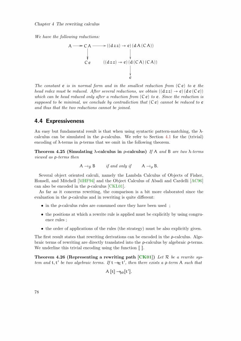
Chapter 4 The rewriting calculus
We have the following reductions:
A // // CA
// ((d z z) _ e) (dA (CA))
Ce ((d z z) _ e) (d (CA) (CA))
e
The constant e is in normal form and in the smallest reduction from (Ce) to e thehead redex must be reduced. After several reductions, we obtain ((d z z) _ e) (d e (Ce))
which can be head reduced only after a reduction from (Ce) to e. Since the reduction issupposed to be minimal, we conclude by contradiction that (Ce) cannot be reduced to eand thus that the two reductions cannot be joined.
4.4 Expressiveness
An easy but fundamental result is that when using syntactic pattern-matching, the λ-calculus can be simulated in the ρ-calculus. We refer to Section 4.1 for the (trivial)encoding of λ-terms in ρ-terms that we omit in the following theorem.
Theorem 4.25 (Simulating λ-calculus in ρ-calculus) If A and B are two λ-termsviewed as ρ-terms then
A→β B if and only if A→ρ B.
Several object oriented calculi, namely the Lambda Calculus of Objects of Fisher,Honsell, and Mitchell [MHF94] and the Object Calculus of Abadi and Cardelli [AC96]can also be encoded in the ρ-calculus [CKL01].
As far as it concerns rewriting, the comparison is a bit more elaborated since theevaluation in the ρ-calculus and in rewriting is quite different:
• in the ρ-calculus rules are consumed once they have been used ;
• the positions at which a rewrite rule is applied must be explicitly by using congru-ence rules ;
• the order of applications of the rules (the strategy) must be also explicitly given.
The first result states that rewriting derivations can be encoded in the ρ-calculus. Alge-braic terms of rewriting are directly translated into the ρ-calculus by algebraic ρ-terms.We underline this trivial encoding using the function J K.
Theorem 4.26 (Representing a rewriting path [CK01]) Let R be a rewrite sys-tem and t, t ′ be two algebraic terms. If t→→R t
′, then there exists a ρ-term A such that
A JtK→→ρδJt′K.
78
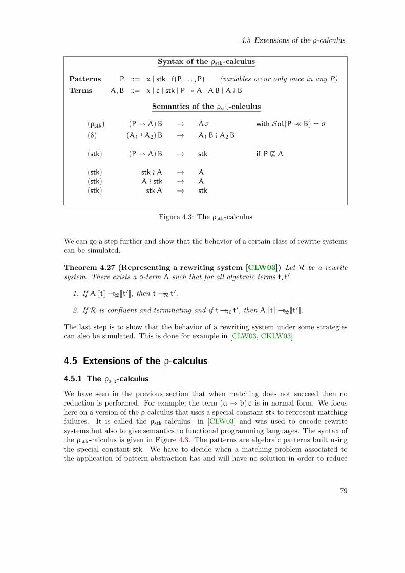
4.5 Extensions of the ρ-calculus
Syntax of the ρstk-calculus
Patterns P ::= x | stk | f(P, . . . , P) (variables occur only once in any P)
Terms A,B ::= x | c | stk | P _ A | AB | A ≀ B
Semantics of the ρstk-calculus
(ρstk) (P _ A)B → Aσ with Sol(P ≺≺ B) = σ
(δ) (A1 ≀ A2)B → A1B ≀ A2B
(stk) (P _ A)B → stk if P 6⊑ A
(stk) stk ≀ A → A
(stk) A ≀ stk → A
(stk) stkA → stk
Figure 4.3: The ρstk-calculus
We can go a step further and show that the behavior of a certain class of rewrite systemscan be simulated.
Theorem 4.27 (Representing a rewriting system [CLW03]) Let R be a rewritesystem. There exists a ρ-term A such that for all algebraic terms t, t ′
1. If A JtK→→ρδJt′K, then t→→R t
′.
2. If R is confluent and terminating and if t→→R t′, then A JtK→→ρδJt
′K.
The last step is to show that the behavior of a rewriting system under some strategiescan also be simulated. This is done for example in [CLW03, CKLW03].
4.5 Extensions of the ρ-calculus
4.5.1 The ρstk-calculus
We have seen in the previous section that when matching does not succeed then noreduction is performed. For example, the term (a _ b) c is in normal form. We focushere on a version of the ρ-calculus that uses a special constant stk to represent matchingfailures. It is called the ρstk-calculus in [CLW03] and was used to encode rewritesystems but also to give semantics to functional programming languages. The syntax ofthe ρstk-calculus is given in Figure 4.3. The patterns are algebraic patterns built usingthe special constant stk. We have to decide when a matching problem associated tothe application of pattern-abstraction has and will have no solution in order to reduce
79

Chapter 4 The rewriting calculus
the term to stk. This is the case when neither an instantiation of the argument nor areduction can make the problem solvable. In other words,
∀σ1, σ2, ∀B′, Bθ1→→ρδB
′ ⇒ Pσ2 6≡ B ′
(P _ A)B→stk stk
Nevertheless, this evaluation rule is not decidable. This is why we introduce a superposi-tion relation 6⊑ between (patterns and) terms whose aim is to characterize a broad classof matching equations that have not and will never have a solution (i.e. independentlyof subsequent instantiations and reductions).
Definition 4.28 (Definitive failures) The relation 6⊑ is defined as follows
stk 6⊑ g(B1, . . . , Bn) if g 6≡ stkstk 6⊑ Q _ B
f(P1, . . . , Pm) 6⊑ g(B1, . . . , Bn) if f 6≡ g or n 6= m or ∃i, Pi 6⊑ Bi
f(P1, . . . , Pm) 6⊑ stkf(P1, . . . , Pm) 6⊑ Q _ B
f(P1, . . . , Pm) 6⊑ (Q _ A)B if Q 6⊑ B or f(P1, . . . , Pm) 6⊑ A
The ρstk-calculus handles uniformly matching failures and eliminates them when theyare not significant for the computation. The semantics of the ρstk-calculus is given inFigure 4.3.
We show on an example how the ρstk-calculus can be used to encode term rewritingsystems and to give semantics to functional programming languages. Further details canbe found in [CLW03].
Example 4.29 (Encoding of the Peano addition) We suppose given the constants0, S, add and rec. We define the following ρ-term
plus , (rec z) _
(
(add 0y) _ y
≀(add (S x)y) _ S (z (rec z) (addxy))
)
addition , n _ m _(
plus (rec plus) (addnm))
The variable z will contain a copy of plus to allow “recursive calls”. We show in Fig-ure 4.4 that this term actually computes the addition over Peano integers.
The notations m, m+n and m−n have to be understood as the terms S(. . . (S 0) . . .)with the right number of S symbols.
The term plus(rec plus) (addnm) can be infinitely reduced but it is weakly normal-ising: the reduction →stk removes the n−1 first attempt to apply the rule (add 0y) _ y
since 0 6⊑ n as soon as n > 0. At the end of the reduction, the step →stk removes thenon-terminating term since S x 6⊑ 0. The normal form m+n (which is actually uniquesince the ρstk-calculus is confluent) is sound.
80

4.5 Extensions of the ρ-calculus
additionnm
→→ρ plus (rec plus) (addnm)
→→ρδ ((add 0y) _ y) (addnm)
≀ ((add (S x)y) _ S (plus (rec plus) (addxy))) (addnm)
→ρ ((add 0y) _ y) (addnm)
≀ S (plus (rec plus) (addn− 1m))
→stk S (plus (rec plus) (addn− 1m))
→→ρδ S
(
((add 0y) _ y) (addn− 1m)
≀ ((add (S x)y) _ S (plus (rec plus) (addxy))) (addn− 1m)
)
...
→→ρδstk S (. . . (S
(
((add 0y) _ y) (add 0m)
≀ ((add (S x)y) _ S (plus (rec plus) (addxy))) (add 0m)
)
) . . .)
→ρδ S (. . . (S
(
m
≀ ((add (S x)y) _ S (plus (rec plus) (addxy))) (add 0m)
)
) . . .)
→stk S (. . . (Sm))
≡ m+n
Figure 4.4: Reduction of a ρ-term encoding the addition
81
Chapter 4 The rewriting calculus
4.5.2 The ρd-calculus
Term rewriting systems and classical guiding strategies have been encoded in the originalrewriting calculus [CK01] and in the ρstk-calculus [CLW03]. The former encoding israther elaborated while the latter is simpler but restricted to convergent (i.e. confluentand strongly normalizing) term rewriting systems. To extend this encoding to arbitraryterm rewrite systems, a new evaluation rule that enriches the semantics of the structureoperator is added and an evaluation strategy is enforced by imposing a certain disciplineon the application of the evaluation rules. This strategy is defined syntactically usingan appropriate notion of value and is used in order to recover confluence of the calculusthat is lost in the general case.
The obtained calculus is the distributive rewriting calculus, called the ρd-calculus andintroduced in [CHW06]. This formalism shares the syntax of the ρstk-calculus and usesthe notion of values that intuitively represent the terms that we do not need to evaluate.These values can be extended to the so-called structure values and stuck values that willbe used to restrict the applications of the evaluation rules.
The syntax and the operational semantics of the ρd-calculus is given in Figure 4.5. Themain difference w.r.t. the ρstk-calculus is the γ rule that although seems very naturaland not dangerous leads to simple non confluent reductions if not restricted to structurevalues [CHW06].
Thanks to the (γ) rule, which defines the right-distributivity of the application overthe structure, we can encode potentially non-confluent TRS in the ρd-calculus (thiscontrasts with the ρstk-calculus). More precisely, given a TRS R we can build the termsΩ1
R and ΩR such that
• Ω1Rm represents (i.e. reduces to) the one-step reducts of m w.r.t. R,
• ΩRm represents the normal forms of m w.r.t. R (if they exist).
4.6 Higher-order matching in the ρ-calculus
In Part I, we studied higher-order matching in the untyped λ-calculus modulo a re-striction of the β-conversion. Now that the ρ-calculus has been introduced, we givea smooth and very short introduction to higher-order matching in the ρ-calculus. Wemainly emphasize some of the problems that are interesting for a future study.
In this section, we use the notations of Chapter 2 and in particular capital lettersdenote matching variables. We call matching in the ρ-calculus the process of finding asubstitution σ of matching variables into ρ-terms such that an equation A ≪ B has asolution if and only if Aσ =ρδ B. In this section, we focus on the role played by theρ-rule and thus we solve equations only modulo this rule.
4.6.1 Matching in the λ-calculus vs matching in the ρ-calculus
We begin with a very simple example: we consider the matching problem
Xa≪ g(a, a)
82

4.6 Higher-order matching in the ρ-calculus
Syntax of the ρd-calculus
Patterns P ::= x | stk | f(P, . . . , P) (variables occur only once in any P)
Terms A,B ::= x | c | stk | P _ A | AB | A ≀ B
Values of the ρd-calculus
V ::= x | c | f(V, . . . , V) | P _ T (Values)
Vγ ::= V | Vγ ≀ Vγ (Structure Values)
Vρδ ::= V | stk (Stuck Values)
Semantics of the ρd-calculus
(βρd) (P _ A) Vρδ → Aσ if Sol(P ≺≺ Vρδ) = σ
(δ) (A1 ≀ A2) Vρδ → A1 V
ρδ ≀ A2 Vρδ
(γ) A (Vγ1 ≀ Vγ
2 ) → A Vγ1 ≀ A Vγ
2
(stk) (P _ A)B → stk if P 6⊑ A
(stk) stk ≀ A → A
(stk) A ≀ stk → A
(stk) stkA → stk
Figure 4.5: The ρd-calculus
In the λ-calculus, this problem has 4 independent solutions given by
λx.g(a, a)/X, λx.g(a, x)/X, λx.g(x, a)/X, λx.g(x, x)/X.
This problem has an extra solution in the ρ-calculus because of its matching capabilities:
a _ g(a, a)/X.
In this example, the matching capabilities of the ρ-calculus give an extra solution.Moreover, some equations have solutions in the ρ-calculus but not in the λ-calculus. Typ-ically, such an equation should instantiate a matching variable by a pattern-abstractionthat “decomposes” its argument. This is the case in the following equation
(
x _ (Xg(x)))
≪ (x _ x)
83

Chapter 4 The rewriting calculus
which has no solution in the λ-calculus whereas the substitution
(g(y) _ y)/X
is a solution in the ρ-calculus.
4.6.2 Matching in the ρ-calculus needs unification
We conjecture that is is not possible to study higher-order matching in the ρ-calculusindependently from unification.
We show on a simple example that there exist matching problems that are equivalentto unification problems.
Consider for example the following matching problem in the ρ-calculus
(f(g(x), y) _ y) f(Zg(a), a) ≪ a
In the body of the pattern-abstraction, the variable x is not used. The problem hasthus as many solutions as there are instantiations of Z such that the match between thereducts of Zg(a) and g(x) succeeds. In other words, we should equivalently solve theunification equation
Zg(a) =ρ g(X)
where X is a fresh variable.
4.6.3 Extensionality in the ρ-calculus
To conclude this section, we give a short discussion on the extensionality of terms (orprograms) defined with pattern-matching that is not yet (to the knowledge of the au-thor) well-understood. We claim that higher-order matching in the ρ-calculus should bedefined as the process that solves of equation modulo ρ(δ). But it is not so clear that, inpractice, this is the right equality one should consider. For example, the two followingterms
g(g(x)) _ x g(x) _ (g(y) _ y) x
should be equal in the same way the two following functional programs
let f z = match z with
g(g(X)) -> X
and
let f z =
match z with
| g(X) -> match X with
| g(Y) -> Y
84

4.6 Higher-order matching in the ρ-calculus
are. But in fact, in the plain ρ-calculus these two terms are distinct normal forms. Atfirst sight, this problem seems easy to solve by adding the equality
c(P1, . . . , Pn) _ M = c(x1, . . . , xn) _ (P1 _ . . . (Pn _ M) xn) . . .) x1
if ∃i, Pi is not a variable
where the variables xi are fresh. Nevertheless, this equality does not make equal theterms
g(x ′) _ f(
(g(x) _ x) x ′, (g(x) _ x) x ′)
and g(g(x)) _ f(x, x)
and this seems to be rather difficult to achieve.
Conclusion
We first give a presentation of the ρ-calculus that makes clear that matching and sub-stitutions are the two fundamental operations of the calculus. We will analyze them inmore detail in the following chapter.
We also show that confluence of the ρ-calculus should be studied with care. In Chap-ter 6, we will study this property and compare the ρ-calculus with other pattern-basedcalculi.
85

Chapter 4 The rewriting calculus
86

Chapter 5
The explicit ρ-calculus
Context The substitution application (inherited from the λ-calculus) and the pattern-matching (inherited from rewriting) are the fundamental operations of the rewritingcalculus.
To perform pattern-matching, evaluation rules of the ρ-calculus use helper functionsthat are indeed implicit computations: all the computations related to the consideredmatching theory belong to the meta-level. These computations are conceptually andcomputationally important in all matching theories, from syntactic ones to quite elabo-rated ones like associative-commutative theories [Eke95]. In concrete implementations,substitutions and pattern-matching should be separated and interact with one another.In particular, we want matching related computations and applications of substitutionsto be explicit.
Explicit substitution λ-calculi [ACCL91, Les94, Mel95, Mel96, Ros96, DG01, Kes07]have been widely studied. They play a central role in some implementations of ML [LN04]and provide nice tools to deal with higher-order unification [DHK00] or to representincomplete proofs in type theory [Mun97].
In this work, we need to make explicit both substitutions and matching computations.
Contributions A first step toward an explicit handling of the matching related com-putations was the introduction of matching problems as part of the ρ-calculus syn-tax [CKL02]. More precisely, the matching constraints represent constrained terms whichare eventually instantiated by the substitution obtained as solution of the correspondingmatching problem (if such a solution exists).
The matching constraints are solved and the resulting substitutions are applied inone step. In concrete implementations these operations the matching constraint solvingand the substitution application) should be separated and should interact with othercomputations. In particular, we want computations on constraints and applications ofconstraints (substitutions) to be explicit.
The evaluation rules solving the syntactic matching problems eventually transform aterm constrained by a matching problem to the same term but constrained by the solvedproblem, that is, by a substitution. The application of the resulting substitutions followsthe approaches used in λ-calculi with explicit substitutions.
In all the explicit substitution calculi, substitutions can be delayed thanks to the β rulethat transforms a β-redex (λx.A)B into the explicit application on A of the substitutionthat replaces x by B. In the explicit ρ-calculus, the application of substitutions is delayed
87

Chapter 5 The explicit ρ-calculus
to the moment where the original matching constraint is solved. Thus, the role of theβ rule is taken by the ρ rule which transforms the application of a rewrite rule into theapplication of a matching constraint and by the evaluation rules solving the obtainedmatching problem. This led to a calculus a la λx-calculus [Ros96] simple and withoutsubstitution compositions.
This calculus [CFK04] handles at the object level not only the matching problems butalso the application of the resulted substitutions. Nevertheless, these two computationsare handled differently and considered one at a time.
We present two versions of the ρ-calculus, one with explicit substitutions and one withexplicit matching, together with a version that combines the two and considers efficiencyissues and more precisely the composition of substitutions. This allows us to isolate thefeatures absolutely necessary in both cases and to analyze the issues related to the twoapproaches. The result is a full calculus that enjoys the usual good properties of explicitsubstitutions (conservativity, termination) and which is confluent. We show that the ρ-calculus, and especially explicit ρ-calculi, are suitable as a useful theoretical back-end forimplementations of rewriting-based languages. This work has been implemented usingthe Tom language [BBK+06] and gives an interpreter for the ρ-calculus.
A first version of this work was published in [CFK04]. A long version close to thischapter was published in [CFK07].
Outline of the chapter Sections 5.1 and 5.2 consider respectively the extensions of theplain ρ-calculus for explicit substitution (ρs) and explicit matching (ρm). Section 5.3presents the combination (ρ
x) of the two previous calculi enriched with a rule for com-
bining term traversal (composition rule for substitutions). Properties such as confluenceof (ρ
x) and the termination of the explicit part are then established in Section 5.4. We
finally give some hints on a direct implementation of explicit ρ-calculi in Section 5.5 andon a ρ-calculus with de Bruijn indices and explicit substitutions in Section 5.6.
5.1 Explicit substitution ρs
We introduce in this section a generalization of the λx-calculus [Ros96] that we callρ-calculus with explicit substitutions and that considers abstractions not only on singlevariables but also on patterns potentially containing several variables. On the otherhand, the obtained ρ-calculus with explicit substitutions, denoted shortly ρs, can beseen as an extension of the plain ρ-calculus with explicit substitutions.
In the plain ρ-calculus, when reducing the application of a rule to a term, the matchingbetween the left-hand side of the rule and the term is solved and the resulting substitutionis applied to the right-hand side of the rule at the meta-level of the calculus. Thismeans that, in one step, we compute the substitution solving the corresponding matchingproblem and apply it.
This reduction can obviously be decomposed into two steps, one computing the sub-stitution and the other one describing the application of this substitution. This decom-position does not mean that the matching related computations and the application of
88
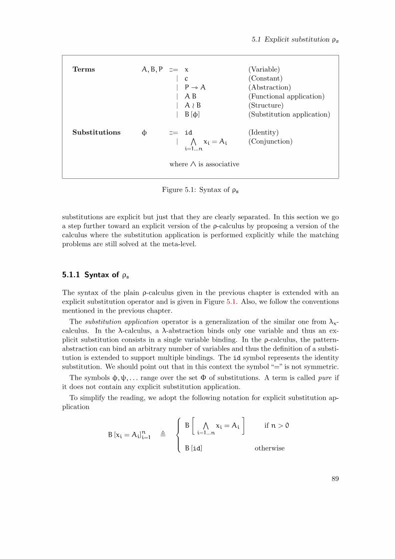
5.1 Explicit substitution ρs
Terms A,B, P ::= x (Variable)| c (Constant)| P _ A (Abstraction)| A B (Functional application)| A ≀ B (Structure)| B [φ] (Substitution application)
Substitutions φ ::= id (Identity)|
∧
i=1...n
xi = Ai (Conjunction)
where ∧ is associative
Figure 5.1: Syntax of ρs
substitutions are explicit but just that they are clearly separated. In this section we goa step further toward an explicit version of the ρ-calculus by proposing a version of thecalculus where the substitution application is performed explicitly while the matchingproblems are still solved at the meta-level.
5.1.1 Syntax of ρs
The syntax of the plain ρ-calculus given in the previous chapter is extended with anexplicit substitution operator and is given in Figure 5.1. Also, we follow the conventionsmentioned in the previous chapter.
The substitution application operator is a generalization of the similar one from λx-calculus. In the λ-calculus, a λ-abstraction binds only one variable and thus an ex-plicit substitution consists in a single variable binding. In the ρ-calculus, the pattern-abstraction can bind an arbitrary number of variables and thus the definition of a substi-tution is extended to support multiple bindings. The id symbol represents the identitysubstitution. We should point out that in this context the symbol “=” is not symmetric.
The symbols φ,ψ, . . . range over the set Φ of substitutions. A term is called pure ifit does not contain any explicit substitution application.
To simplify the reading, we adopt the following notation for explicit substitution ap-plication
B [xi = Ai]ni=1 ,
B
[
∧
i=1...n
xi = Ai
]
if n > 0
B [id] otherwise
89
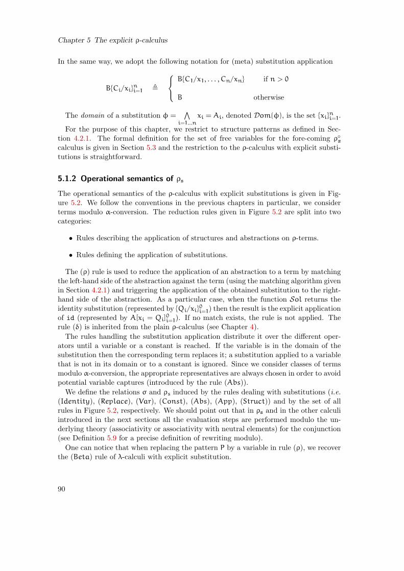
Chapter 5 The explicit ρ-calculus
In the same way, we adopt the following notation for (meta) substitution application
BCi/xini=1 ,
BC1/x1, . . . , Cn/xn if n > 0
B otherwise
The domain of a substitution φ =∧
i=1...n
xi = Ai, denoted Dom(φ), is the set xini=1.
For the purpose of this chapter, we restrict to structure patterns as defined in Sec-tion 4.2.1. The formal definition for the set of free variables for the fore-coming ρ
x
calculus is given in Section 5.3 and the restriction to the ρ-calculus with explicit substi-tutions is straightforward.
5.1.2 Operational semantics of ρs
The operational semantics of the ρ-calculus with explicit substitutions is given in Fig-ure 5.2. We follow the conventions in the previous chapters in particular, we considerterms modulo α-conversion. The reduction rules given in Figure 5.2 are split into twocategories:
• Rules describing the application of structures and abstractions on ρ-terms.
• Rules defining the application of substitutions.
The (ρ) rule is used to reduce the application of an abstraction to a term by matchingthe left-hand side of the abstraction against the term (using the matching algorithm givenin Section 4.2.1) and triggering the application of the obtained substitution to the right-hand side of the abstraction. As a particular case, when the function Sol returns theidentity substitution (represented by Qi/xi
0i=1) then the result is the explicit application
of id (represented by A[xi = Qi]0i=1). If no match exists, the rule is not applied. The
rule (δ) is inherited from the plain ρ-calculus (see Chapter 4).
The rules handling the substitution application distribute it over the different oper-ators until a variable or a constant is reached. If the variable is in the domain of thesubstitution then the corresponding term replaces it; a substitution applied to a variablethat is not in its domain or to a constant is ignored. Since we consider classes of termsmodulo α-conversion, the appropriate representatives are always chosen in order to avoidpotential variable captures (introduced by the rule (Abs)).
We define the relations σ and ρs induced by the rules dealing with substitutions (i.e.(Identity), (Replace), (Var), (Const), (Abs), (App), (Struct)) and by the set of allrules in Figure 5.2, respectively. We should point out that in ρs and in the other calculiintroduced in the next sections all the evaluation steps are performed modulo the un-derlying theory (associativity or associativity with neutral elements) for the conjunction(see Definition 5.9 for a precise definition of rewriting modulo).
One can notice that when replacing the pattern P by a variable in rule (ρ), we recoverthe (Beta) rule of λ-calculi with explicit substitution.
90

5.1 Explicit substitution ρs
(P _ A) B →ρ A [xi = Ci]ni=1
where Sol(P ≺≺ B) = Ci/xini=1
(A1 ≀ A2) B →δ A1 B ≀ A2 B
A [id] →Identity A
x [φ∧ (x = A) ∧ψ] →Replace A
y [φ] →Var y if y 6∈ Dom(φ)
c [φ] →Const c
(P _ A) [φ] →Abs P [φ] _ A [φ]
(A B) [φ] →App A [φ] B [φ]
(A ≀ B) [φ] →Struct A [φ] ≀ B [φ]
Figure 5.2: Operational semantics of ρs
Example 5.1 (Application of a rewrite rule) In order to compute the disjunctivenormal form of a propositional formula, we use the rewrite rule
not(and(x, y)) _ or(not(x), not(y)).
The application of this rewrite rule to the term not(and(t, f)) is described in ρs by thefollowing reduction
(
not(and(x, y)) _ or(not(x), not(y)))
not(and(t, f))→ρ or(not(x), not(y)) [x = t ∧ y = f]→→App (or [x = t ∧ y = f])(not(x [x = t ∧ y = f]), not(y [x = t ∧ y = f]))→Const or(not(x [x = t ∧ y = f]), not(y [x = t ∧ y = f]))→→Replace or(not(t), not(f))
Example 5.2 (Multiple applications) Since substitutions cannot be composed, theapplication of each substitution is done independently and can involve a lot of evaluationsteps needed in order to access to the leaves of the term (seen as a tree).
(g(x) _ ((f(y) _ h(x, y)) f(a)) g(b)
→ρ ((f(y) _ h(x, y)) f(a)) [x = b]
→ρ h(x, y) [y = a] [x = b]
→→σ h(x, y [y = a]) [x = b]
→→σ h(x, a) [x = b]
→→σ h(x [x = b], a)
→→σ h(b, a)
As we will see later on, if the substitutions are composed, then the term traversal relatedsteps can be factorized (see Example 5.8).
91
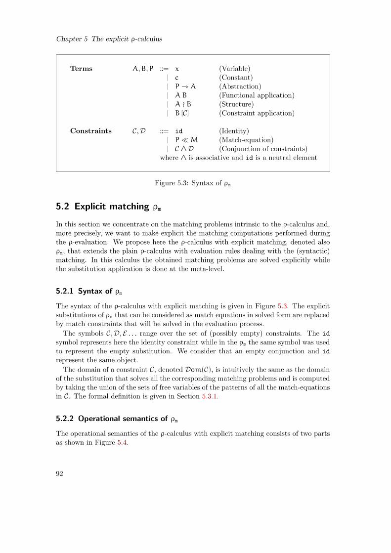
Chapter 5 The explicit ρ-calculus
Terms A,B, P ::= x (Variable)| c (Constant)| P _ A (Abstraction)| A B (Functional application)| A ≀ B (Structure)| B [C] (Constraint application)
Constraints C,D ::= id (Identity)| P ≪M (Match-equation)| C ∧ D (Conjunction of constraints)
where ∧ is associative and id is a neutral element
Figure 5.3: Syntax of ρm
5.2 Explicit matching ρm
In this section we concentrate on the matching problems intrinsic to the ρ-calculus and,more precisely, we want to make explicit the matching computations performed duringthe ρ-evaluation. We propose here the ρ-calculus with explicit matching, denoted alsoρm, that extends the plain ρ-calculus with evaluation rules dealing with the (syntactic)matching. In this calculus the obtained matching problems are solved explicitly whilethe substitution application is done at the meta-level.
5.2.1 Syntax of ρm
The syntax of the ρ-calculus with explicit matching is given in Figure 5.3. The explicitsubstitutions of ρs that can be considered as match equations in solved form are replacedby match constraints that will be solved in the evaluation process.
The symbols C,D, E . . . range over the set of (possibly empty) constraints. The id
symbol represents here the identity constraint while in the ρs the same symbol was usedto represent the empty substitution. We consider that an empty conjunction and id
represent the same object.
The domain of a constraint C, denoted Dom(C), is intuitively the same as the domainof the substitution that solves all the corresponding matching problems and is computedby taking the union of the sets of free variables of the patterns of all the match-equationsin C. The formal definition is given in Section 5.3.1.
5.2.2 Operational semantics of ρm
The operational semantics of the ρ-calculus with explicit matching consists of two partsas shown in Figure 5.4.
92

5.2 Explicit matching ρm
As for ρs, the first part describes the application of structures and abstractions on ρ-terms. This time the (ρ) rule always applies and reduces the application of an abstractionto a term constraint by the corresponding matching problem.
The matching problems are handled by the second part of the evaluation rules thatare clearly inspired by the ones presented in Section 4.2.1. A matching constraint issimplified using the decomposition rules which are strongly related to the consideredmatching theory. As we have already mentioned, we consider only structures of algebraicterms as patterns and we restrict to a decidable and unitary matching theory and, moreprecisely, to syntactic matching. Therefore, we do not handle the higher-order symbols(e.g. “_”, “≪”) and we only decompose the restricted patterns. The two decompositionrules given in Figure 5.4 are thus performed w.r.t. to an empty matching theory for thestructure operator and for the constant symbols. Since an empty conjunction and id
represent the same object and thus, the rule (DecomposeF ) can be used for constants(i.e. n = 0) in which case the result is the identity.
When a part of the constraint is solved and independent of the rest of the constraint,the corresponding substitution can be applied at the meta-level. We consider that themeta-application of the substitution A/x to the term B, denoted BA/x, is higher-orderand thus performs α-conversion in order to avoid the possible variable captures. Thecondition in rule (ToSubst) guarantees that a matching problem is solved and thus (partof) the corresponding substitution can be applied only if all its variables are assignedthe same term. Non-linear matching problems can lead to matching constraints whichassign different terms to the same variable and which represent, intuitively, a failure (seeExample 5.5). The doubletons in a matching constraint are eliminated with the rule(Idem).
Notice that in the rule (ToSubst), because of the hygiene-convention, the intersectionbetween the set of free variables of A and Dom(C ∧D) is empty and thus, the variablesin A cannot be captured in the right-hand side of the rule.
The ρ-calculus (and in particular ρm) is well-suited to deal with (matching) errors,represented by constraints without solution, that is, constraints that do not representsubstitutions. Depending on the intended use of the calculus we may want or not topropagate such (constraint) failures. If the failures are propagated, the error’s locationis lost and the final result would be a term with constraints with no solution applied oneach leaf of the term (considered as a tree). The information contained in such a termseems useless when one wants to analyze the error and, for debugging reasons, we donot want to lose the error’s location. This is why the failures are not propagated as theyare but only the corresponding substitution (if one exists) is propagated.
Example 5.3 (Application of a rewrite rule) The term presented in Example 5.1
93
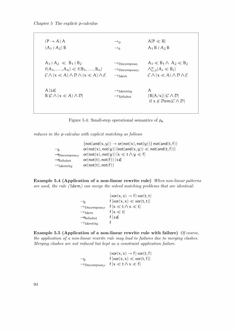
Chapter 5 The explicit ρ-calculus
(P _ A)A →ρ A[P ≪ B]
(A1 ≀ A2) B →δ A1 B ≀ A2 B
A1 ≀ A2 ≪ B1 ≀ B2 →Decompose≀ A1 ≪ B1 ∧ A2 ≪ B2
f(A1, . . . , An) ≪ f(B1, . . . , Bn) →DecomposeF ∧ni=1(Ai ≪ Bi)
C ∧ (x≪ A) ∧ D ∧ (x≪ A) ∧ E →Idem C ∧ (x≪ A) ∧ D ∧ E
A [id] →Identity A
B [C ∧ (x≪ A) ∧ D] →ToSubst (BA/x) [C ∧ D]
if x 6∈ Dom(C ∧ D)
Figure 5.4: Small-step operational semantics of ρm
reduces in the ρ-calculus with explicit matching as follows
(
not(and(x, y)) _ or(not(x), not(y)))
not(and(t, f))→ρ or(not(x), not(y)) [not(and(x, y)) ≪ not(and(t, f))]→→DecomposeF or(not(x), not(y)) [x≪ t ∧ y≪ f]→→ToSubst or(not(t), not(f)) [id]
→Identity or(not(t), not(f))
Example 5.4 (Application of a non-linear rewrite rule) When non-linear patternsare used, the rule ( Idem) can merge the solved matching problems that are identical:
(xor(x, x) _ f) xor(t, t)→ρ f [xor(x, x) ≪ xor(t, t)]→DecomposeF f [x≪ t ∧ x≪ t]→Idem f [x≪ t]→→ToSubst f [id]
→Identity f
Example 5.5 (Application of a non-linear rewrite rule with failure) Of course,the application of a non-linear rewrite rule may lead to failures due to merging clashes.Merging clashes are not reduced but kept as a constraint application failure.
(xor(x, x) _ f) xor(t, f)→ρ f [xor(x, x) ≪ xor(t, f)]→DecomposeF f [x≪ t ∧ x≪ f]
94

5.3 Explicit substitution and explicit matching ρx
The next example illustrates the usefulness of explicit matching when we want to trackthe source (cause) of the failure.
Example 5.6 (Run-time error: matching failure) Let us consider the following rulethat checks if two persons are brothers, i.e., if they have the same father:
Brother(Person(Name(x),Father(z)),Person(Name(y),Father(z))) _ t
When checking if two concrete persons (Alice and Bob) are brothers by applying thisrule to the corresponding term:
Brother(Person(Name(Alice),Father(John)), Person(Name(Bob),Father(Jim)))
we obtain as result the term
t [z≪ John∧ z≪ Jim]
indicating that the variable z corresponding to the father cannot be instantiated correctly,i.e., that the father of the two persons is not the same.
This is in contrast with the ρ-calculus with explicit substitutions where the fact thatthe application of the rule to the term is in normal form indicates that the matching hasno solution but gives no information on the source of this failure.
5.3 Explicit substitution and explicit matching ρx
The combination of the two previously introduced calculi, ρs and ρm, leads to a versionof the calculus that handles explicitly the matching constraints resolution as well as theapplication of the substitutions. This calculus, called ρx and introduced in [CFK04]does not handle the composition of substitutions, a key issue when one wants to obtainefficient implementations.
In what follows we add this feature and define ρx. The properties of this calculus are
then studied.
5.3.1 Syntax of ρx
The syntax presented in Figure 5.5 merges the ones of ρs and ρm and defines ρx-terms.
In what follows we refer to the three categories of ρx-terms by simply calling them terms,
substitutions and constraints respectively.One can notice that the conjunction operator ∧ is overloaded and it is used to build
substitutions as well as constraints. Since the two types of conjunctions are disjoint, inwhat follows, we will generally denote the corresponding identities ids and idm by thesame symbol id.
We assume that the functional, substitution and constraint application operators as-sociate to the left, while the other operators associate to the right. The priority ofthe substitution application is higher than that of the constraint application which ishigher than that of the functional application. The application has a higher priority than
95

Chapter 5 The explicit ρ-calculus
Terms A,B, P ::= x (Variables)| c (Constants)| P _ A (Abstraction)| A B (Functional application)| A ≀ B (Structure)| B [φ] (Substitution application)| B [C] (Constraint application)
Substitutions φ,ψ ::= ids (Identity)| x = A (Equation)| φ∧ψ (Conjunction of equations)
Constraints C,D ::= idm (Identity)| P ≪ A (Match-equation)| C ∧ D (Conjunction of constraints)
where ∧ is associativeand ids and idm are neutral elements
Figure 5.5: Syntax of ρx
96
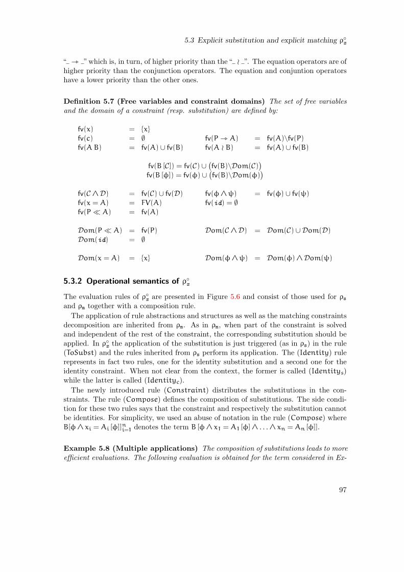
5.3 Explicit substitution and explicit matching ρx
“ _ ”which is, in turn, of higher priority than the“ ≀ ”. The equation operators are ofhigher priority than the conjunction operators. The equation and conjuntion operatorshave a lower priority than the other ones.
Definition 5.7 (Free variables and constraint domains) The set of free variablesand the domain of a constraint (resp. substitution) are defined by:
fv(x) = x
fv(c) = ∅ fv(P _ A) = fv(A)\fv(P)fv(A B) = fv(A) ∪ fv(B) fv(A ≀ B) = fv(A) ∪ fv(B)
fv(B [C]) = fv(C) ∪(
fv(B)\Dom(C))
fv(B [φ]) = fv(φ) ∪(
fv(B)\Dom(φ))
fv(C ∧ D) = fv(C) ∪ fv(D) fv(φ∧ψ) = fv(φ) ∪ fv(ψ)
fv(x = A) = FV(A) fv(id) = ∅fv(P ≪ A) = fv(A)
Dom(P ≪ A) = fv(P) Dom(C ∧ D) = Dom(C) ∪ Dom(D)
Dom(id) = ∅
Dom(x = A) = x Dom(φ∧ψ) = Dom(φ) ∧ Dom(ψ)
5.3.2 Operational semantics of ρx
The evaluation rules of ρx
are presented in Figure 5.6 and consist of those used for ρsand ρm together with a composition rule.
The application of rule abstractions and structures as well as the matching constraintsdecomposition are inherited from ρm. As in ρm, when part of the constraint is solvedand independent of the rest of the constraint, the corresponding substitution should beapplied. In ρ
xthe application of the substitution is just triggered (as in ρs) in the rule
(ToSubst) and the rules inherited from ρs perform its application. The (Identity) rulerepresents in fact two rules, one for the identity substitution and a second one for theidentity constraint. When not clear from the context, the former is called (Identitys)while the latter is called (Identityc).
The newly introduced rule (Constraint) distributes the substitutions in the con-straints. The rule (Compose) defines the composition of substitutions. The side condi-tion for these two rules says that the constraint and respectively the substitution cannotbe identities. For simplicity, we used an abuse of notation in the rule (Compose) whereB[φ∧ xi = Ai [φ]]ni=1 denotes the term B [φ∧ x1 = A1 [φ] ∧ . . .∧ xn = An [φ]].
Example 5.8 (Multiple applications) The composition of substitutions leads to moreefficient evaluations. The following evaluation is obtained for the term considered in Ex-
97

Chapter 5 The explicit ρ-calculus
(P _ A) B →ρ A[P ≪ B]
(A1 ≀ A2) B →δ A1 B ≀ A2 B
A1 ≀ A2 ≪ B1 ≀ B2 →Decompose≀ A1 ≪ B1 ∧ A2 ≪ B2
f(A1, . . . , An) ≪ f(B1, . . . , Bn) →DecomposeF ∧ni=1(Ai ≪ Bi)
C ∧ (x≪ A) ∧ D ∧ (x≪ A) ∧ E →Idem C ∧ (x≪ A) ∧ D ∧ E
B [C ∧ (x≪ A) ∧ D] →ToSubst (B [x = A]) [C ∧ D]
if x 6∈ Dom(C ∧ D)
A [id] →Id A
x [φ∧ (x = A) ∧ψ] →Replace A
y [φ] →Var y if y 6∈ Dom(φ)
c [φ] →Const c
(P _ A) [φ] →Abs P [φ] _ A [φ]
(A B) [φ] →App A [φ] B [φ]
(A ≀ B) [φ] →Struct A [φ] ≀ B [φ]
(A[Pi ≪ Bi]ni=1) [φ] →Constraint (A [φ])[Pi [φ] ≪ Bi [φ]]ni=1
if n > 0
(B[xi = Ai]ni=1) [φ] →Compose B[φ∧ xi = Ai [φ]]ni=1
if n > 0
Figure 5.6: Small-step operational semantics of ρx
98

5.4 Properties of ρx
ample 5.2.(g(x) _ ((f(y) _ h(x, y)) f(a))) g(b)
→→ ((f(y) _ h(x, y)) f(a)) [x = b]
→→ h(x, y) [y = a] [x = b]
→Compose h(x, y) [x = b∧ y = a [x = b]]
→Const h(x, y) [x = b∧ y = a]
→→App h(x [x = b∧ y = a], y [x = b∧ y = a])
→→Replace h(b, a)
All the evaluation steps dealing with the traversal of the term h(x, y) are done only oncethis time since only one substitution should be propagated.
The non-efficient route given in Example 5.2 can also be taken but while this was the onlyalternative for ρs, this problem disappears for ρ
xif we apply the evaluation rules with
a strategy [BKK96] that gives the highest priority to the composition rule, a canonicalway to limit term traversal.
As mentioned at the beginning of this section, a ρ-calculus handling explicitly the con-straint solving and the substitution application was coined for the first time in [CFK04].In ρx there was no mechanism for the composition of substitutions (i.e. no (Compose)rule) and consequently, no substitution conjunctions. Therefore, we can consider ρx asa restriction of ρ
xwhere all substitutions are simple equations and the (Compose) rule
is not available.
5.4 Properties of ρx
5.4.1 Proof scheme
As mentioned before, all the evaluation steps are performed modulo the theory of theconjunction (in ρ
xmodulo the associativity and the neutral elements) and thus, we are
performing rewriting modulo a set of axioms. We give first a formal definition for thisevaluation and then we introduce a more operational evaluation that is usually used inproofs and implementations. For a detailed exposition about rewriting modulo, we referto [Hue80, JK86, KK99, Ohl98].
Definition 5.9 ((R/A)) Given a rewrite system R and a set of axioms A, the term t
(R/A)-rewrites to t ′, denoted t →R/A t′, if there exists a rule l → r ∈ R, a term u, an
occurrence q in u and a substitution σ such that t∗←→A u[q ← σ(l)] and t ′
∗←→A u[q ←σ(r)] where u[q ← v] denotes the term u with the sub-term at the position q replaced byv.
Definition 5.10 ((R,A)) Given a rewrite system R and a set of axioms A , the term t
(R,A)-rewrites to a term t ′, which is denoted by t→R,A t′ if there exists a rule l→ r ∈ R,
a position q in t, and a substitution σ such that t|q∗←→A σ(l) (i.e. the sub-term of t
at position q is equivalent to σ(l)), and t ′ = t[q ← σ(r)] (i.e. t ′ is equal to t where thesub-term at the position q is replaced by σ(r)).
99
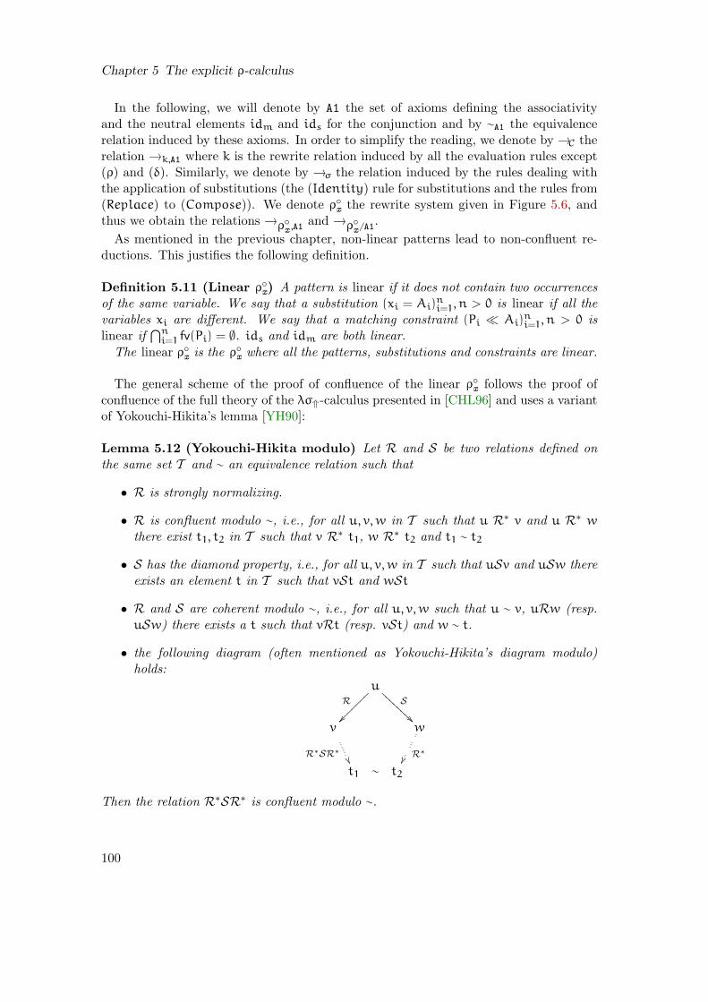
Chapter 5 The explicit ρ-calculus
In the following, we will denote by A1 the set of axioms defining the associativityand the neutral elements idm and ids for the conjunction and by ∼A1 the equivalencerelation induced by these axioms. In order to simplify the reading, we denote by→C therelation →k,A1 where k is the rewrite relation induced by all the evaluation rules except(ρ) and (δ). Similarly, we denote by →σ the relation induced by the rules dealing withthe application of substitutions (the (Identity) rule for substitutions and the rules from(Replace) to (Compose)). We denote ρ
xthe rewrite system given in Figure 5.6, and
thus we obtain the relations →ρx,A1
and →ρx/A1
.
As mentioned in the previous chapter, non-linear patterns lead to non-confluent re-ductions. This justifies the following definition.
Definition 5.11 (Linear ρx) A pattern is linear if it does not contain two occurrences
of the same variable. We say that a substitution (xi = Ai)ni=1, n > 0 is linear if all the
variables xi are different. We say that a matching constraint (Pi ≪ Ai)ni=1, n > 0 is
linear if⋂n
i=1 fv(Pi) = ∅. ids and idm are both linear.
The linear ρx
is the ρx
where all the patterns, substitutions and constraints are linear.
The general scheme of the proof of confluence of the linear ρx
follows the proof ofconfluence of the full theory of the λσ⇑-calculus presented in [CHL96] and uses a variantof Yokouchi-Hikita’s lemma [YH90]:
Lemma 5.12 (Yokouchi-Hikita modulo) Let R and S be two relations defined onthe same set T and ∼ an equivalence relation such that
• R is strongly normalizing.
• R is confluent modulo ∼, i.e., for all u, v,w in T such that u R∗ v and u R∗ w
there exist t1, t2 in T such that v R∗ t1, w R∗ t2 and t1 ∼ t2
• S has the diamond property, i.e., for all u, v,w in T such that uSv and uSw thereexists an element t in T such that vSt and wSt
• R and S are coherent modulo ∼, i.e., for all u, v,w such that u ∼ v, uRw (resp.uSw) there exists a t such that vRt (resp. vSt) and w ∼ t.
• the following diagram (often mentioned as Yokouchi-Hikita’s diagram modulo)holds:
uR
~~~~
~~~
S
AAA
AAAA
A
v
R∗SR∗
w
R∗
t1 ∼ t2
Then the relation R∗SR∗ is confluent modulo ∼.
100

5.4 Properties of ρx
Proof. Since the coherence properties are strong, to go from the classical lemma givenin [CHL96] to this generalization is just a straightforward verification. We only have touse these coherence properties as much as needed to “factorize” the coherence relationat the bottom of all commutative diagrams given in [CHL96]. In fact, we first prove byinduction on the R-depth that:
uR∗
~~~~
~~~
S
AAA
AAAA
A
v
R∗SR∗
w
R∗
t1 ∼ t2
Then we conclude by induction on the R-depth of u, and where we distinguish betweenthe depth zero and nonzero. The following diagram holds for the case zero
uS //
S
u1
S
R∗
// u2
R∗SR∗
u ′ S //
R∗
u ′1
R∗
R∗
// u ′2
R∗
∼ u ′3
R∗
vR∗SR∗
// v1 ∼ v2R∗
// v3 ∼ v4 ∼ v5
and confluence follows since R is coherent with ∼ and thus v1 ∼ v2 R∗ v3 can be replacedby v1 R∗ v ′3 ∼ v3.
The diagram for the induction case is more complex but is handled similarly.
We thus split the evaluation rules of ρx
into two relations corresponding to the relationsR and S of the previous lemma. A natural choice for the relation R is →C . In fact, therules dealing with constraints and explicit substitutions should be strongly normalizingand confluent (in explicit substitution calculi we always ask these properties for theexplicit part). The relation S cannot be the rewrite relation induced by the (ρ) and (δ)rules since this relation verifies neither the diamond property (the (δ) rule duplicatesredexes) nor the Yokouchi-Hikita’s diagram modulo (the relation →C duplicates alsoredexes). This is why we use a parallelization of the (ρ), (δ) rules.
We first prove in Section 5.4.3 the termination of →C . Then we prove that →C isconfluent, taking into account the fact that the rules can be applied modulo the associa-tivity and the neutral elements (ids, idm) for the conjunctions. Then we formally definethe parallelization of (ρ) and (σ) and show that it verifies the diamond property (Sec-tion 5.4.5). Finally, we prove the Yokouchi-Hikita’s diagram modulo and conclude theproof of confluence of the linear ρ
xby noticing that the parallelization and the original
relation have the same transitive closure.First of all, we show the soundness of the explicit substitution reductions, a mandatory
and useful lemma in any calculus involving explicit substitution.
101
Chapter 5 The explicit ρ-calculus
5.4.2 Soundness of explicit substitutions
First, we show that →σ is confluent and strongly normalizing and thus defines a func-tion σ on terms. Secondly, we show that explicit substitutions soundly relate to metasubstitutions. The corollary is that the function σ associates to every term a pure term(where all the substitutions have been applied).
Lemma 5.13 (Convergence of →σ) In the linear ρx, the relation→σ is confluent and
strongly normalizing.
Proof. The relation →σ is strongly normalizing by Lemma 5.22 which proves a moregeneral result that is, the termination of →C . The local confluence is easily proved byobserving that all critical pairs modulo A1 are convergent and as a consequence of theabove properties, confluence is obtained. We must notice that the linearity conditionis mandatory since for example the non-linear substitution application x [x = a∧ x = b]
leads either to a or to b.
Lemma 5.14 (Soundness of explicit substitutions) For all n, for all terms Ai andB, there exists a term B ′ such that
B [xi = Ai]ni=1 →→C B ′Ai/xi
ni=1 and B→→C B
′
Proof. If n = 0 then the result follows by the application of the (Identity) rule. Other-wise, we proceed by induction on B.
• If B is a variable, then if this variable is one of the xi for i between 1 and n thenapply the (Replace) rule. If not, then apply the (Var) rule.
• If B is an application, then B1 B2 [xi = Ai]ni=1 can be reduced using the (App) rule
to B1 [xi = Ai]ni=1 B2 [xi = Ai]
ni=1. Then, the result follows by induction.
• If B is a substitution application, then
B ′[xi = Ai]ni=1 [φ] →Compose B ′[φ∧ xi = Ai [φ]]ni=1
≡ (1) B ′φ,Aiφ/xini=1
≡ (2) B ′φAiφ/xini=1
≡ (3) B ′Ai/xini=1φ
The first step (1) is the application of the induction hypothesis twice. The secondstep is valid since by α-conversion we can suppose that all the xi do not belong tothe free variables of Ai. The third step is exactly the substitution lemma of theplain ρ-calculus (xi 6∈ fv(Ai)).
• The other cases are similar to the application one.
102
5.4 Properties of ρx
5.4.3 Termination of the constraint handling rules
First of all, we will show that →C is strongly normalizing and for this we use the lex-icographic product of two orders. The first order is a measure (a size) on terms suchthat the size of the right-hand side is smaller than that of the left-hand side for the rules(ToSubst), (Idem), (Replace), and the decomposition rules and equal for all the otherrules. The second order is based on a polynomial interpretation which decreases on allthe other rules.
The measure on terms defined below represents (an upper bound of) the size of thecorresponding pure term where all the pending substitutions were applied. The size ofa term B [x = A] is thus the size of B plus the size of A multiplied by the number ofoccurrences of x is B (called here the multiplicity of x in B), taking thus into account thepossible instantiation(s) of x by A in B. As far as it concerns the matching constraints,we have to take into account that they can (possibly) become substitutions. We makethus an approximation and consider that for the terms of the form B [P ≪ A], eachvariable of P is (potentially) instantiated by a sub-term of A that is approximated by A.
This measure is preserved by the duplicative rules (e.g. the term (x ≀ x) [φ] and its(Struct) reduct x [φ] ≀ x [φ] have the same size independently of φ). Notice also thatin the right-hand side of the rule (ToSubst), A is not affected by the variables of thedomain of C ∧ D (by α-conversion) and thus, the size decreases (see Lemma 5.19).
Definition 5.15 (Multiplicity) The multiplicity of the variable x in the term A, de-noted Ax (A), is defined inductively in Figure 5.7.
Definition 5.16 (Size) The size of a term A, denoted S(A), is defined in Figure 5.8.
We should point out that the notions of multiplicity and size are compatible w.r.t. toneutrality of the conjunction operator since id has no impact on the two notions. It isalso compatible w.r.t. the associativity of the conjunction and w.r.t. α-conversion.
Lemma 5.17 (Soundness of multiplicity) For any term A and variable x such thatx 6∈ fv(A) we have Ax (A) = 0.
Proof. By induction on the structure of A.
• A = y with x 6= y. By definition.
• A = c. By definition.
• A = P _ A1. We have Ax (P _ A1) = Ax (A1) and the result holds by applyingthe induction hypothesis.
• A = A1A2. Then Ax (A1A2) = Ax (A1)+Ax (A2) and the result holds by applyingtwice the induction hypothesis since x 6∈ fv(A1A2) implies x 6∈ fv(A1), x 6∈ fv(A2).
• A = A1 ≀ A2. Similar to the previous case.
103
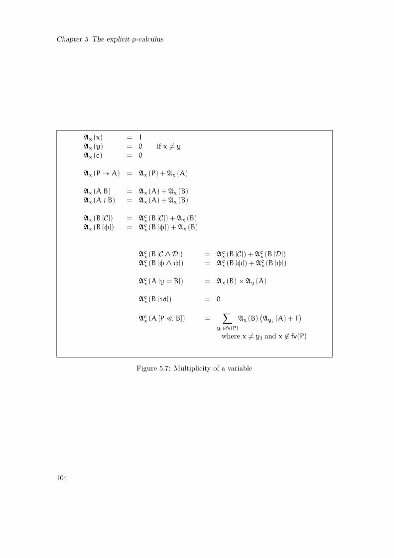
Chapter 5 The explicit ρ-calculus
Ax (x) = 1
Ax (y) = 0 if x 6= y
Ax (c) = 0
Ax (P _ A) = Ax (P) + Ax (A)
Ax (A B) = Ax (A) + Ax (B)
Ax (A ≀ B) = Ax (A) + Ax (B)
Ax (B [C]) = Acx (B [C]) + Ax (B)
Ax (B [φ]) = Acx (B [φ]) + Ax (B)
Acx (B [C ∧ D]) = Ac
x (B [C]) + Acx (B [D])
Acx (B [φ∧ψ]) = Ac
x (B [φ]) + Acx (B [ψ])
Acx (A [y = B]) = Ax (B) × Ay (A)
Acx (B [id]) = 0
Acx (A [P ≪ B]) =
∑
yj∈fv(P)
Ax (B)(
Ayj(A) + 1
)
where x 6= yj and x 6∈ fv(P)
Figure 5.7: Multiplicity of a variable
104
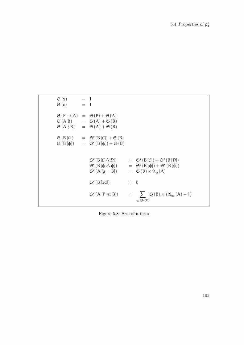
5.4 Properties of ρx
S(x) = 1
S(c) = 1
S(P _ A) = S (P) + S (A)
S (A B) = S (A) + S (B)
S (A ≀ B) = S (A) + S (B)
S (B [C]) = Sc (B [C]) + S (B)
S (B [φ]) = Sc (B [φ]) + S (B)
Sc (B [C ∧ D]) = Sc (B [C]) + Sc (B [D])
Sc (B [φ∧ψ]) = Sc (B [φ]) + Sc (B [ψ])
Sc (A [y = B]) = S (B) × Ay (A)
Sc (B [id]) = 0
Sc (A [P ≪ B]) =∑
yj∈fv(P)
S(B) ×(
Ayj(A) + 1
)
Figure 5.8: Size of a term
105
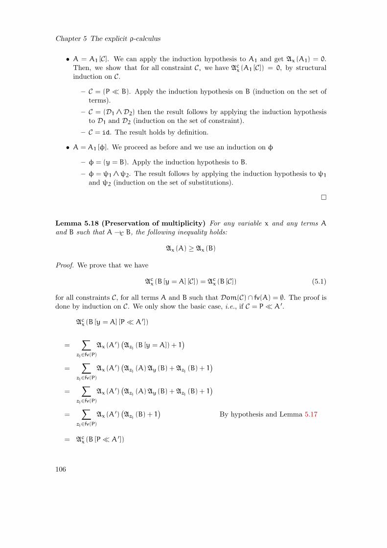
Chapter 5 The explicit ρ-calculus
• A = A1 [C]. We can apply the induction hypothesis to A1 and get Ax (A1) = 0.Then, we show that for all constraint C, we have Ac
x (A1 [C]) = 0, by structuralinduction on C.
– C = (P ≪ B). Apply the induction hypothesis on B (induction on the set ofterms).
– C = (D1 ∧ D2) then the result follows by applying the induction hypothesisto D1 and D2 (induction on the set of constraint).
– C = id. The result holds by definition.
• A = A1 [φ]. We proceed as before and we use an induction on φ
– φ = (y = B). Apply the induction hypothesis to B.
– φ = ψ1 ∧ψ2. The result follows by applying the induction hypothesis to ψ1
and ψ2 (induction on the set of substitutions).
Lemma 5.18 (Preservation of multiplicity) For any variable x and any terms Aand B such that A→C B, the following inequality holds:
Ax (A) ≥ Ax (B)
Proof. We prove that we have
Acx (B [y = A] [C]) = Ac
x (B [C]) (5.1)
for all constraints C, for all terms A and B such that Dom(C) ∩ fv(A) = ∅. The proof isdone by induction on C. We only show the basic case, i.e., if C = P ≪ A ′.
Acx (B [y = A] [P ≪ A ′])
=∑
zj∈fv(P)
Ax (A ′)(
Azj(B [y = A]) + 1
)
=∑
zj∈fv(P)
Ax (A ′)(
Azj(A) Ay (B) + Azj
(B) + 1)
=∑
zj∈fv(P)
Ax (A ′)(
Azj(A) Ay (B) + Azj
(B) + 1)
=∑
zj∈fv(P)
Ax (A ′)(
Azj(B) + 1
)
By hypothesis and Lemma 5.17
= Acx (B [P ≪ A ′])
106

5.4 Properties of ρx
One can notice that the condition x 6∈ fv(A) is not needed since the multiplicities in Aonly depend on the variables in the domain of C (and not on x).
We can also prove by an easy induction on n that if x does not belong to ∪ni=1fv(Pi)
and if for all i, x 6= yi then
Ax
(
B
[
∧
i=1..n
Pi ≪Mi
])
= Ax (B) +
n∑
i=1
∑
xj∈fv(Pi)
Ax (Ai) ×(
Axj(B) + 1
)
(5.2)
Ax
(
B
[
∧
i=1..n
yi = Ai
])
= Ax (B) +
n∑
i=1
Ax (Ai) × Axi(B) (5.3)
Since the multiplicity is defined by a monotonic induction it is sufficient to prove theresult when the reduction takes place at the root of A. We give all the computations inFigure 5.9.
Lemma 5.19 (Preservation of size) For any terms A and B such that A →C B, thefollowing inequality holds:
S(A) ≥ S(B)
The inequality is strict if the reduction is done using either the ( ToSubst) rule, or the(Replace) rule, or the ( Idem) rule, or the decomposition rules.
Proof. The proof of the lemma is similar to that of Lemma 5.18. We only give somecases.
(Replace) S (x [φ∧ x = A∧ψ])
= S (x) + Sc (x [φ]) + Sc (x [x = A]) + Sc (x [ψ])
= 1+ Sc (x [φ]) + S (A) × Ax (x) + Sc (x [ψ])
> S(A)
(ToSubst) S (x [C ∧ (x≪ A) ∧ D])
= S (x) + Sc (x [C ∧ (x≪ A) ∧ D])
= S (x) + Sc (x [C]) + Sc (x [x≪ A]) + Sc (x [D])
> 1+ S (A) × Ax (x)
> S(A)
(Idem) S (B [C ∧ (x≪ A) ∧ D ∧ (x≪ A) ∧ E ])
= S (B) + Sc (B [C]) + 2Sc (B [x≪ A]) + Sc (B [D]) + Sc (B [E ])
> S(B) + Sc (B [C]) + Sc (B [x≪ A]) + Sc (B [D]) + Sc (B [E ])
= S (B [C ∧ (x≪ A) ∧ τ∧ D])
107

Chapter 5 The explicit ρ-calculus
(Identity) Ax (M [id])
= Acx (A [id]) + Ax (A)
= Ax (A)
(Replace) Ax (y [φ ∧ y = A ∧ ψ])
= Ax (y) + Acx (y [φ ∧ y = A ∧ ψ])
= Ax (y) + Acx (y [φ]) + Ac
x (y [y = A]) + Acx (y [ψ])
≥ Acx (y [y = A])
= Acx (A) × Ay (y)
= Acx (A)
(Const) Ax (c [φ])
= Ax (c) + Acx (c [φ])
≥ Ax (c)
(Abs) Ax ((A _ B) [φ])
= Acx ((A B) [φ]) + Ax (A _ B)
= Acx (A [φ]) + Ax (B) + Ac
x (A [φ]) + Ax (B)
= Ax (A [φ] _ B [φ])
(App) Ax ((A B) [φ])
= Acx ((A B) [φ]) + Ax (A B)
= Acx (A [φ]) + Ax (B) + Ac
x (A [φ]) + Ax (B)
= Ax (A [φ] B [φ])
(Constraint) Ax
`
A[Pi ≪ Bi ]ni=1 [xj = Aj ]
m
i=1
´
= Ax (A[Pi ≪ Bi ]ni=1) +
∑jAx (Aj) Axj
(A[Pi ≪ Bi ]ni=1)
Eq. 5.2= Ax (A) +
∑i
∑yj∈fv(Pi) Ax (Bi) × Ayj
(A) +∑
iAc
x ((A [Pi ≪ Bi ]) [φ])
=∑
i
∑yj∈fv(Pi) Ax (Bi) × Ayj
(A) +∑
iAc
x ((A [Pi ≪ Bi ]) [φ])
=∑
i
∑yj∈fv(Pi)(Ax (Bi) + Ac
x (Bi [φ])) × (Ayj(A) + Ac
yj(A [φ]))
=∑
i
∑yj∈fv(Pi) Ax (Bi [φ]) × Ayj
(A [φ])
= Ax (A [φ][Pi ≪ Bi [φ]]ni=1)
(Compose) Ax
`
B[xj = Aj ]mj=1 [xi = Ai ]
ni=1
´
Eq. 5.3= Ax
`
B[xj = Aj ]mj=1
´
+∑
iAx (Ai) Axi
`
B[xj = Aj ]mj=1
´
Eq. 5.3= Ax (B) +
∑jAx (Aj) Axj
(B) +∑
iAx (Ai)
`
Axi(B) +
∑jAxi
(Aj) Axj(B)
´
= Ax (B) +∑
iAx (Ai) Axi
(B) +∑
jAxj
(B)`
Ax (Aj) +∑
iAx (Aj) Axi
(Aj)´
= Ax (B) +∑
iAx (Ai) Axi
(B) +∑
jAx (Aj [xi = Ai ]
ni=1)
Eq. 5.3= Ax
“
ˆ
xi = Ai ∧ xj = Aj [xi = Ai ]n
i=1
˜
i,j(B)
”
(ToSubst) Ax (B [C ∧ (y≪ A) ∧ D])
= Ax (B) + Acx (B [C ∧ (y≪ A) ∧ D])
= Ax (B) + Acx (B [C]) + Ac
x (B [y≪ A]) + Acx (B [D])
= Ax (B) + Acx (B [C]) + Ax (A) × (Ay (B) + 1) + Ac
x (B [D])
> Ax (B) + Acx (B [C]) + Ax (A) × Ay (B) + Ac
x (B [D])Eq. 5.1
= Ax (B) + Acx (B [y = A] [C]) + Ax (A) × Ay (B) + Ac
x (B [y = A] [D])
= Ax (B [y = A]) + Acx (B [y = A] [C ∧ D])
= Ax (B [y = A] [C ∧ D])
Figure 5.9: Preservation of multiplicity
108

5.4 Properties of ρx
Definition 5.20 (Polynomial interpretation) We use the standard order on naturalnumbers in order to define the following polynomial interpretation:
I(k) = 3 I(P _ B) = I(P) + I(B) + 1
I(A ≀ B) = I(A) + I(B) + 1 I(A B) = I(A) + I(B) + 1
I(B [C]) = I (C) + I(B) + 1 I(A [φ]) = (I (φ) + 2) × I(A)
I (C ∧ D) = I (C) + I (D) I (φ∧ψ) = I (φ) + I (ψ)
I (id) = 0 I (x = A) = I(A)
I (P ≪ A) = I(P) + I(A)
We should point out that the polynomial interpretation is compatible w.r.t. to neutral-ity of the conjunction operator since id has no impact on the two notions. It is alsocompatible w.r.t. the associativity of the conjunction and w.r.t. α-conversion. Moreover,since the addition and the multiplication are increasing on naturals, the monotonicitycondition a > b implies I(a) > I(b) is clearly satisfied. We show that for any terms Aand B such that A →C B the image of A is greater than that of B for any replacementof the interpretation of the variables of A and B by naturals bigger than 2.
Lemma 5.21 For any terms A and B such that A →C B using either (Compose), or(Constraint), or (Abs), or (Const), or (Var), or ( Identity), or (App), or (Struct)then
I(A) > I(B)
Proof. For any natural number n, for any terms B,Ai for any patterns Pi and for anyvariables yi the following equalities hold:
I(B
[
∧
i=1..n
Pi ≪ Ai
]
) = I(B) + 1+∑
i
(I(Pi) + I(Ai)) (5.4)
I(B
[
∧
i=1..n
yi = Ai
]
) = I(B) ×
(
2+∑
i
I(Ai)
)
(5.5)
We can first remark that for any constraint C (resp. substitution φ) we have I(C) ≥ 0
(resp. I(φ) ≥ 0) and for any term A we have I(A) > 2.We check the inequality for each rule mentioned in the Lemma in Figure 5.10.
Lemma 5.22 (SN of →C) The relation →C is strongly normalizing.
Proof. Every pair of terms in→C (strictly) decreases the lexicographic product (S () , I( )).
109

Chapter 5 The explicit ρ-calculus
(Identitys) I(A [ids]) = (I (ids) + 2) × I(A) = 2× I(A) > I(A)
(Identityc) I(A [idc]) = I (idc) + I(A) + 1 = I(A) + 1 > I(A)
(Var) I(y [φ]) = (I (φ) + 2) × I(y) > I(y)
(Const) I(c [φ]) = (I (φ) + 2) × I(c) > I(c)
(Abs) I((P _ A) [φ]) = (I (φ) + 2) × I(P _ A)
= (I (φ) + 2) × (I(P) + I(A) + 1)
> (I (φ) + 2) × I(P) + (I (φ) + 2) × I(A) + 1
= I(P [φ]) + I(A [φ]) + 1
= I(P [φ] _ A [φ])
(App) I((AN) [φ]) = (I (φ) + 2) × I(AN)
= (I (φ) + 2) × (I(A) + I(N) + 1)
> (I (φ) + 2) × I(A) + (I (φ) + 2) × I(N) + 1
= I(A [φ]) + I(N [φ]) + 1
= I(A [φ]N [φ])
(Struct) I((A ≀ N) [φ]) = (I (φ) + 2) × I(A ≀ N) + 1= (I (φ) + 2) × (I(A) + I(N) + 1) + 1> (I (φ) + 2) × I(A) + 1+ (I (φ) + 2) × I(N) + 1
= I(A [φ]) + I(N [φ]) + 1= I(A [φ] ≀ N [φ])
(Constraint) I(A[Pi ≪ Ni]ni=1 [φ])
Eq. 5.4= (I (φ) + 2) × (I(A) +
∑i I(Pi) +
∑i I(Ni) + 1)
>∑
i((I(φ) + 2) × I(Pi)) +∑
i((I(φ) + 2) × I(Ni)) + I(φ) + I(A) + 1
=∑
i(I(Pi [φ]) + I(Ni [φ])) + I(φ) + I(A) + 1
=∑
i I(Pi [φ] ≪ Ni [φ]) + I(A [φ]) + 1
= I(A [φ][Pi [φ] ≪ Ni [φ]]ni=1)
(Compose) I(N [xi = Ai]n
i=1 [φ])
= (I(φ) + 2) × I(N [xi = Ai]n
i=1)Eq. 5.5
= (I(φ) + 2) × (∑
i I(Ai) + 2) × I(N)= I(N) × (2× (I(φ) + 2) + (I(φ) + 2) ×
∑i I(Ai))
> I(N) × (I(φ) + 2+ (I(φ) + 2) ×∑
i I(Ai))
= I(N) × (I(φ) + 2+∑
i I(Ai [φ]))
= I(N) (I(φ) + 2+∑
i I(xi = Ai [φ]))
=(
I(φ∧∧
i
(
xi = Ai [φ])
) + 2)
× I(N)
= I(N [φ∧ xi = Ai [φ]]n
i=1)
Figure 5.10: Strict decrease of polynomial interpretation
110
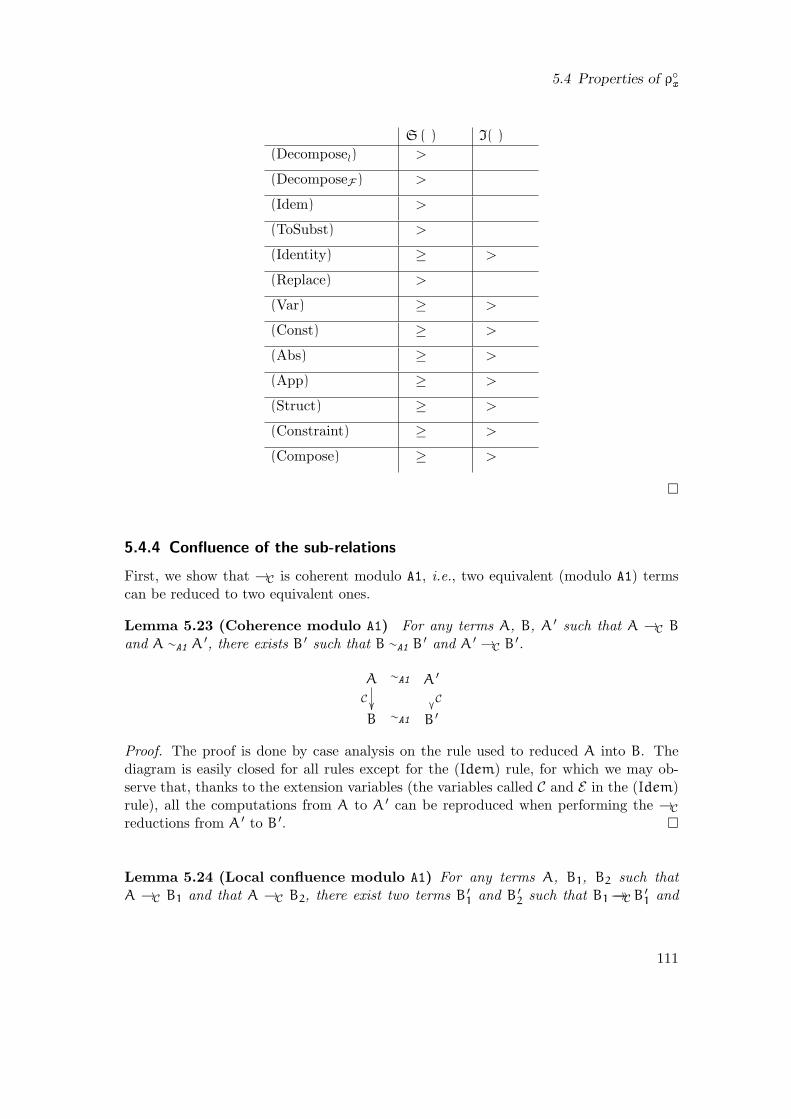
5.4 Properties of ρx
S( ) I( )
(Decompose≀) >
(DecomposeF ) >
(Idem) >
(ToSubst) >
(Identity) ≥ >
(Replace) >
(Var) ≥ >
(Const) ≥ >
(Abs) ≥ >
(App) ≥ >
(Struct) ≥ >
(Constraint) ≥ >
(Compose) ≥ >
5.4.4 Confluence of the sub-relations
First, we show that →C is coherent modulo A1, i.e., two equivalent (modulo A1) termscan be reduced to two equivalent ones.
Lemma 5.23 (Coherence modulo A1) For any terms A, B, A ′ such that A →C B
and A ∼A1 A′, there exists B ′ such that B ∼A1 B
′ and A ′ →C B′.
A
C
∼A1 A ′
CB ∼A1 B ′
Proof. The proof is done by case analysis on the rule used to reduced A into B. Thediagram is easily closed for all rules except for the (Idem) rule, for which we may ob-serve that, thanks to the extension variables (the variables called C and E in the (Idem)rule), all the computations from A to A ′ can be reproduced when performing the →C
reductions from A ′ to B ′.
Lemma 5.24 (Local confluence modulo A1) For any terms A, B1, B2 such thatA →C B1 and that A →C B2, there exist two terms B ′
1 and B ′2 such that B1→→C B
′1 and
111
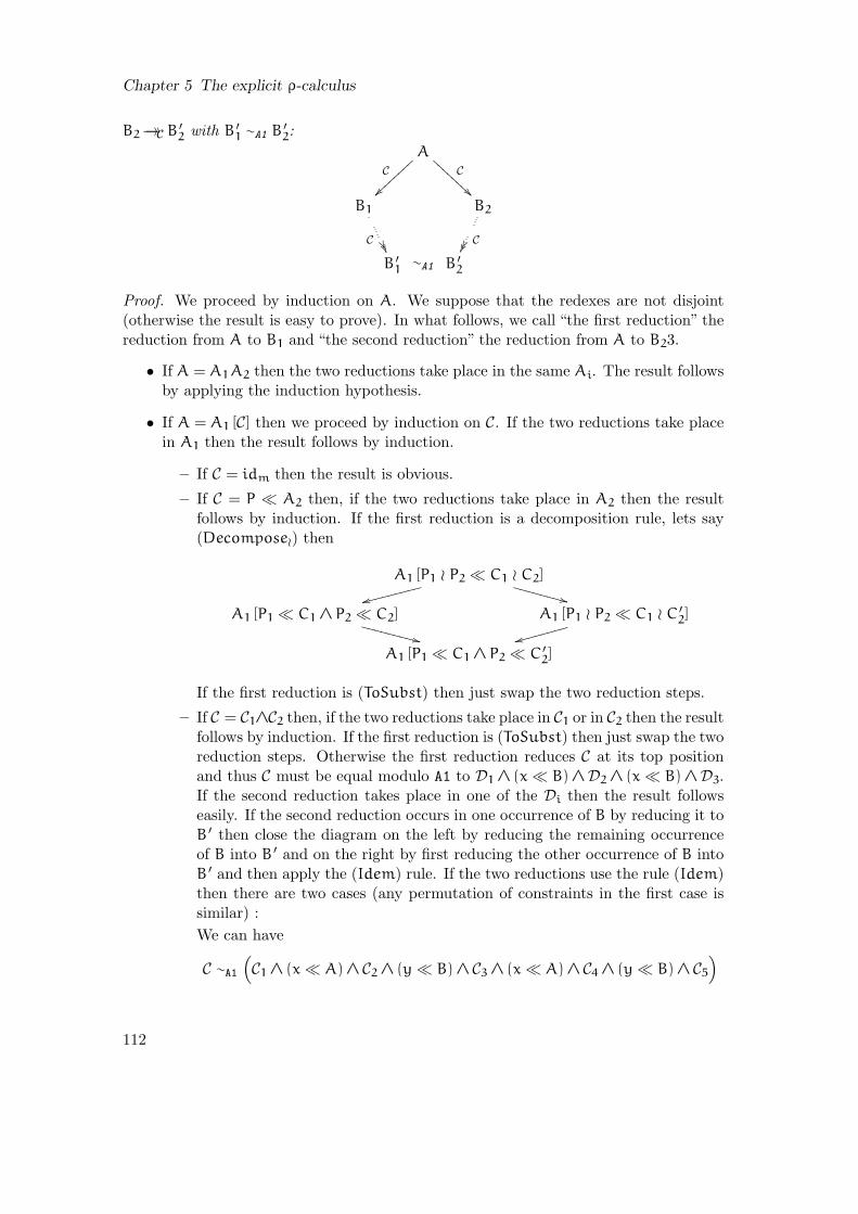
Chapter 5 The explicit ρ-calculus
B2→→C B′2 with B ′
1 ∼A1 B′2:
AC
~~
C
AAA
AAAA
A
B1
C
B2
CB ′
1∼A1 B ′
2
Proof. We proceed by induction on A. We suppose that the redexes are not disjoint(otherwise the result is easy to prove). In what follows, we call “the first reduction” thereduction from A to B1 and “the second reduction” the reduction from A to B23.
• If A = A1A2 then the two reductions take place in the same Ai. The result followsby applying the induction hypothesis.
• If A = A1 [C] then we proceed by induction on C. If the two reductions take placein A1 then the result follows by induction.
– If C = idm then the result is obvious.
– If C = P ≪ A2 then, if the two reductions take place in A2 then the resultfollows by induction. If the first reduction is a decomposition rule, lets say(Decompose≀) then
A1 [P1 ≀ P2 ≪ C1 ≀ C2]
ssggggggggg++VVVVVVVV
A1 [P1 ≪ C1 ∧ P2 ≪ C2]
++WWWWWWWWWA1 [P1 ≀ P2 ≪ C1 ≀ C ′
2]
sshhhhhhhh
A1 [P1 ≪ C1 ∧ P2 ≪ C ′2]
If the first reduction is (ToSubst) then just swap the two reduction steps.
– If C = C1∧C2 then, if the two reductions take place in C1 or in C2 then the resultfollows by induction. If the first reduction is (ToSubst) then just swap the tworeduction steps. Otherwise the first reduction reduces C at its top positionand thus C must be equal modulo A1 to D1 ∧ (x≪ B) ∧ D2 ∧ (x≪ B) ∧ D3.If the second reduction takes place in one of the Di then the result followseasily. If the second reduction occurs in one occurrence of B by reducing it toB ′ then close the diagram on the left by reducing the remaining occurrenceof B into B ′ and on the right by first reducing the other occurrence of B intoB ′ and then apply the (Idem) rule. If the two reductions use the rule (Idem)then there are two cases (any permutation of constraints in the first case issimilar) :
We can have
C ∼A1
(
C1 ∧ (x≪ A) ∧ C2 ∧ (y≪ B) ∧ C3 ∧ (x≪ A) ∧ C4 ∧ (y≪ B) ∧ C5
)
112

5.4 Properties of ρx
and the first reduction eliminates the doubletons related to x and the secondreduction eliminates the doubletons related to y. Then, to close the dia-gram simply swap the two reductions (this is possible thanks to the extensionvariables in the (Idem) rule).
Otherwise
C ∼A1
(
C1 ∧ (x≪ A) ∧ C2 ∧ (x≪ A) ∧ C3 ∧ (x≪ A) ∧ C4
)
and conclude the case as in the previous case.
• If A = A1 [φ] then we proceed by induction on φ and by case analysis on the ruleused for the first reduction.
The interesting case is when the first reduction uses the (Constraint) rule and thesecond reduction is done using the (ToSubst) rule. In this case, the result followsusing the (Compose) rule and Lemma 5.14. Let us denote ∧i(Pi ≪ Bi) by C and∧j(Pj ≪ Bj) by D. In the following we simply write C [x = B] for ∧i(Pi [x = B] ≪Bi [x = B]). Let us suppose moreover that A1 = A3 [C ∧ (y≪ A2) ∧ D] in whichcase the first reduction gives:
(A3 [C ∧ (y≪ A2) ∧ D]) [x = B]
→Constraint A3 [x = B] [C [x = B] ∧ (y [x = B] ≪ A2 [x = B]) ∧ D [x = B]]
→Var A3 [x = B] [C [x = B] ∧ (y≪ A2 [x = B]) ∧ D [x = B]]
→ToSubst A3 [x = B] [y = A2 [x = B]] [C [x = B] ∧ D [x = B]]
→Compose A3 [y = A2 [x = B] ∧ x = B [y = A2 [x = B]]] [C [x = B] ∧ D [x = B]]
By α-conversion, y 6∈ fv(B) and so, by applying Lemma 5.14, we get
→→C A3 [y = A2 [x = B] ∧ x = B ′] [C [x = B] ∧ D [x = B]] (1)
with B→→C B′. The second reduction gives:
(A3 [C ∧ (y≪ A2) ∧ D]) [x = B]
→ToSubst (A3 [y = A2] [C ∧ D]) [x = B]
→Constraint A3 [y = A2] [x = B] [C [x = B] ∧ D [x = B]]
→Compose A3 [x = B∧ y = A2 [x = B]] [C [x = B] ∧ D [x = B]]
→→C A3 [x = B ′ ∧ y = A2 [x = B]] [C [x = B] ∧ D [x = B]] (2)
Lemma 5.14 concludes the case showing that the terms (1) and (2) have a commonreduct.
113

Chapter 5 The explicit ρ-calculus
Lemma 5.25 The relation →C is confluent modulo A1.
Proof. We actually prove a stronger property, that is that the relation is Church-Rosser modulo A1, which is obtained according to [Ohl98] from the strong normalization(Lemma 5.22), the coherence (Lemma 5.23) and the local confluence (Lemma 5.24) mod-ulo A1 of →C .
5.4.5 Parallel version of the ρδ
The parallelization of the ρ and δ rules is an easy extension of the parallel reduction ofTait and Martin-Lof given in Part I. The definition is here a bit longer because of themany congruence rules.
Definition 5.26 (Parallelization of ρδ) The parallelization of the relation induced bythe rules (ρ) and ( δ), denoted ⇒ρδ, is defined inductively in Figure 5.11.
Lemma 5.27 (Diamond Property of ⇒ρδ) For any terms A,B1, B2 there exists aterm A ′ such that the following diagram holds:
Aρδq
~~||||
|||| ρδq
BBB
BBBB
B
B1
ρδq AA
AA B2
ρδq~~
A ′
Proof. The relation ⇒ρδ is the parallelization of an orthogonal system.
5.4.6 Yokouchi-Hikita’s diagram modulo and confluence of ρx
Lemma 5.28 (Yokouchi-Hikita’s diagram modulo) For any terms A, B1 and B2
in the linear ρx
there exists the terms A ′1, A
′2 such that the following diagram holds:
A
C
ρδq
>>>
>>>>
>>>
B1
C∗ ρδq C∗
--
-- B2
C∗
A ′1
∼A1 A ′2
114

5.4 Properties of ρx
A⇒ρδ A′ B⇒ρδ B
′
(P _ A) B⇒ρδ A′[P ≪ B ′]
A ′1⇒ρδ A
′1 A2⇒ρδ A
′2 B⇒ρδ B
′
(A1 ≀ A2) B⇒ρδ A′1 B
′ ≀ A ′2 B
′
A⇒ρδ A
A⇒ρδ A′
P _ A⇒ρδ P _ A ′
A⇒ρδ A′ B⇒ρδ B
′
A B⇒ρδ A′ B ′
A⇒ρδ A′ B⇒ρδ B
′
A ≀ B⇒ρδ A′ ≀ B ′
C ⇒ρδ C ′ A⇒ρδ A′
A [C]⇒ρδ A′ [C ′]
φ⇒ρδ φ′ A⇒ρδ A
′
A [φ]⇒ρδ A′ [φ ′]
B⇒ρδ B′
(P ≪ B)⇒ρδ (P ≪ B ′)
B⇒ρδ B′
(x = B)⇒ρδ (x = B ′)
C ⇒ρδ C ′ D ⇒ρδ D ′
C ∧ D ⇒ρδ C ′ ∧ D ′
φ⇒ρδ φ′ ψ⇒ρδ ψ
′
φ∧ψ⇒ρδ φ′ ∧ψ ′
Figure 5.11: Parallel version of the ρδ-rules
115
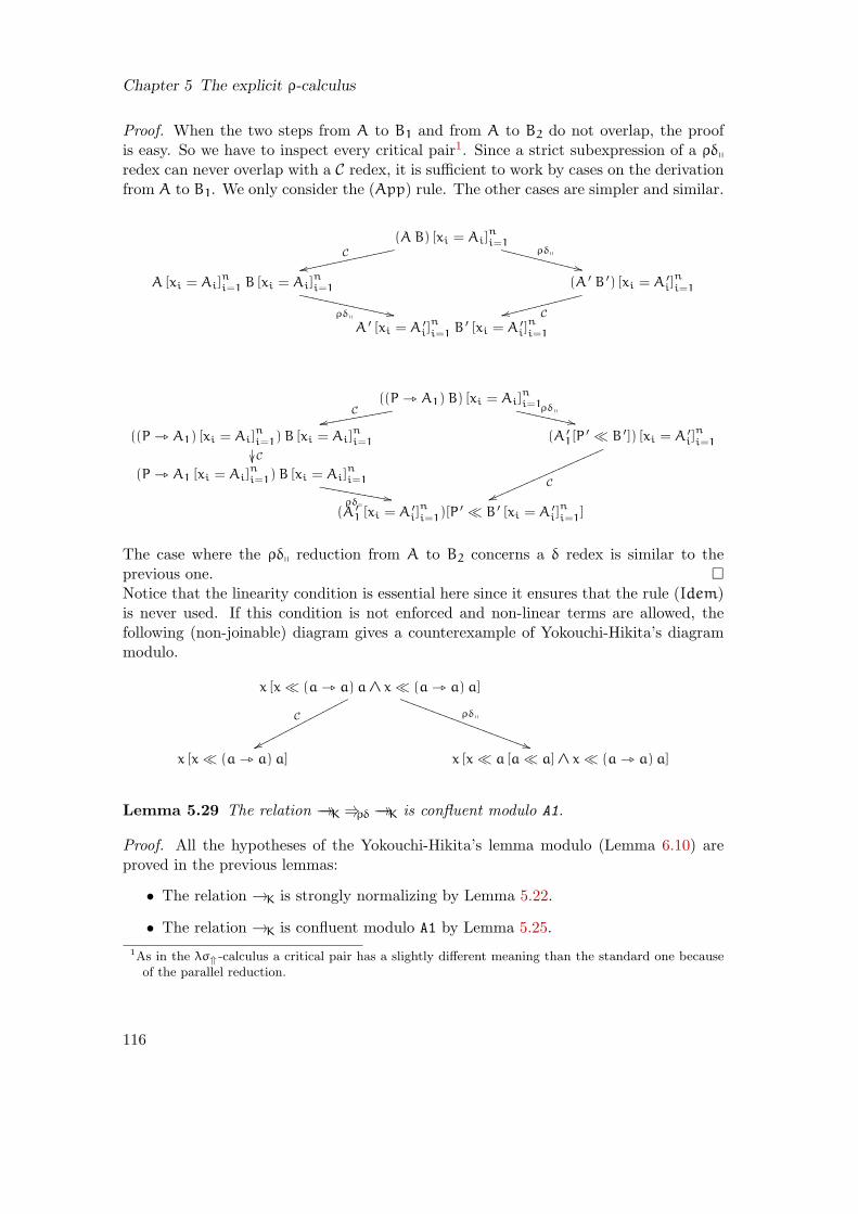
Chapter 5 The explicit ρ-calculus
Proof. When the two steps from A to B1 and from A to B2 do not overlap, the proofis easy. So we have to inspect every critical pair1. Since a strict subexpression of a ρδq
redex can never overlap with a C redex, it is sufficient to work by cases on the derivationfrom A to B1. We only consider the (App) rule. The other cases are simpler and similar.
(A B) [xi = Ai]n
i=1C
rrffffffffffffff ρδq
++WWWWWWWWWWWW
A [xi = Ai]n
i=1 B [xi = Ai]n
i=1
ρδq,,XXXXXXXXXXXXXX
(A ′ B ′) [xi = A ′
i]n
i=1
Cssgggggggggggg
A ′ [xi = A ′
i]n
i=1B ′ [xi = A ′
i]n
i=1
((P _ A1) B) [xi = Ai]n
i=1C
rreeeeeeeeeee ρδq
++XXXXXXXXX
((P _ A1) [xi = Ai]n
i=1) B [xi = Ai]n
i=1
C
(A ′
1[P ′ ≪ B ′]) [xi = A ′
i]n
i=1
C
vvmmmmmmmmmmmmmmmmmm
(P _ A1 [xi = Ai]n
i=1) B [xi = Ai]n
i=1
ρδq
,,YYYYYYYYYYY
(A ′
1 [xi = A ′
i]n
i=1)[P ′ ≪ B ′ [xi = A ′
i]n
i=1]
The case where the ρδq reduction from A to B2 concerns a δ redex is similar to theprevious one. Notice that the linearity condition is essential here since it ensures that the rule (Idem)is never used. If this condition is not enforced and non-linear terms are allowed, thefollowing (non-joinable) diagram gives a counterexample of Yokouchi-Hikita’s diagrammodulo.
x [x≪ (a _ a) a∧ x≪ (a _ a) a]
C
wwpppppppppppppppρδq
))SSSSSSSSSSSSSSSSSSSS
x [x≪ (a _ a) a] x [x≪ a [a≪ a] ∧ x≪ (a _ a) a]
Lemma 5.29 The relation →→K⇒ρδ→→K is confluent modulo A1.
Proof. All the hypotheses of the Yokouchi-Hikita’s lemma modulo (Lemma 6.10) areproved in the previous lemmas:
• The relation →K is strongly normalizing by Lemma 5.22.
• The relation →K is confluent modulo A1 by Lemma 5.25.
1As in the λσ⇑ -calculus a critical pair has a slightly different meaning than the standard one because
of the parallel reduction.
116

5.5 Implementation in the Tom language
• The relation ⇒ρδ has the diamond property by Lemma 5.27.
• The relations →K and ⇒ρδ are coherent modulo A1 : the coherence of ⇒ρδ moduloA1 is obvious and the coherence of →K is obtained by Lemma 5.23.
• Yokouchi-Hikita’s diagram modulo holds by Lemma 5.28.
Lemma 5.30 The relation →ρx,A1
is confluent modulo A1.
Proof. We have→ρδ ⊆⇒ρδ ⊆ →→ρδ thus→ρx,A1
⊆→→K⇒ρδ→→K ⊆→→ρx,A1
and the reflexive
and transitive closure of (→→K ⇒ρδ →→K) is equal to →→ρx,A1
. Then confluence modulo A1
of →ρx,A1
is equivalent to confluence modulo A1 of →→K⇒ρδ→→K. Lemma 5.29 concludes
the proof.
Theorem 5.31 The linear ρx
is confluent (the relation →ρx/A1
is confluent).
Proof. The property follows from the previous lemma and the coherence of→ρx,A1
mod-
ulo ∼A1 [Ohl98].
5.5 Implementation in the Tom language
Explicit substitution calculi have been studied from different points of view. Differentcalculi have been proposed so as to obtain meta properties like confluence and preser-vation of strong normalization [Les94, Ros96, CHL96, DG01]. They have been used toperform higher-order unification [DHK00] just like to represent incomplete proofs in typetheory [Mun97] or to prove correctness of compiler optimizations [Ler02]. Moreover, ex-plicit substitution calculi have been used in two significant practical systems [Nad02]:the Standard ML of New Jersey compiler and the Teyjus implementation of LambdaProlog. In particular the use of de Bruijn indices and the ability to merge togetherstructure traversals (i.e. the composition of substitutions) have a strong positive impacton the system performances [LN04].
The study of explicit ρ-calculi is thus also important for future implementations oflanguages based on the ρ-calculus. Actually, the ρ-calculus provides the basis for alanguage combining functional languages and rewrite based languages (Elan, Maude . . . )features and thus besides provides a toy interpreter allowing us to experiment withthe ρ-calculus. Our implementation of explicit ρ-calculi is a first step toward such alanguage. Moreover, the ρ-calculus provides proof terms for the proof assistants basedon superdeduction [BHK07, Wac05] such as Lemuridae.
The rest of the section is devoted to the brief presentation of our implementationand of the support language, Tom. The gap between the different calculi defined in the
117
Chapter 5 The explicit ρ-calculus
previous sections and the actual implementation is rather small and so, we mainly focushere on the key features of Tom that led to a natural implementation of the explicitρ-calculi.
Following the experience of Elan, a strategic rewriting based language [BKK+98b,KK04], the Tom language extends Java with the purpose of providing high level con-structs inspired by the rewriting community such as powerful matching capabilities alongwith a rich strategy language inspired by Elan and Stratego [Vis01a]. A full presentationof Tom2 is out of the scope of this chapter but we refer to [BBK+06] for a detailedpresentation.
First, Tom performs associative and unitary matching (unlike Elan that performs as-sociative and commutative matching) also known as list matching. Constraints andsubstitutions are represented by lists of atomic matching equations (built using the op-erator “≪”) and respectively equations (built using the operator “ = ”).
Secondly, the overall evaluation process of a term with respect to a rewrite systemand a given strategy can be implemented straightforwardly in Tom since one can defineseparately the rewrite system and the strategy to evaluate it. This is a good way toobtain a modular and easily maintainable implementation.
Thirdly, thanks to an intensive use of the Tom component called Gom [Rei06] thatautomatically generates tree-like data-structures (following [BMV05] and [BJKO00]),we obtain for free the corresponding maximal sharing representation of terms for a givensignature. Maximal sharing has strong impact on performances. For example, we cantest the equality of terms in constant time (check the equality of memory addresses).
Lastly, an elaborated parser was easily obtained by the combination of Tom and asecond generation parser generator such as Antlr : the parser generator is used forparsing, Tom is used for term construction.
The implementation of the operational semantics of the ρx
follows the overall eval-uation process given earlier. All previously given examples can be simulated by theimplementation. Our interpreter is available on the ρ-calculus web page3.
The approach followed here is to give a simple but trustable interpreter for the ρ-calculus. There are other implementations of the ρ-calculus but that are quite different.
iRho It is an interpreter an imperative version of the ρ-calculus [LS04]. The approachis quite different from the one presented in this chapter since the final objective is tomake an agile programming language. The interesting point is that the core of thisimplementation (evaluator) is certified using the proof assistant Coq [Coq07].
Rogue It is an imperative rewriting language that extends the untyped ρ-calculus withmutable expression attributes. The approach is quite different since the main objectiveis to implement efficient decision procedures [SDK+03]. This leads to the developmentof a calculus of explicit binding [SS04] in which the arrow operator of the ρ-calculus
2http://tom.loria.fr3http://rho.loria.fr/implementations.html
118

5.6 Explicit substitutions with generalized de Bruijn indices in the ρ-calculus
is analyzed into two operators: a scoping operator alpha, which binds a variable in anexpression; and a weaker form of arrow showing how to transform expressions matchinga pattern. This is a particular case of dynamic patterns described in Chapter 6.
5.6 Explicit substitutions with generalized de Bruijn indices inthe ρ-calculus
Until now, we do not deal explicitly with α-conversion. There are many works that shouldbe considered: deBruijn [Bru78] indices, the λ-calculus with explicit scoping [HO03],director strings [Sin05] etc. These works should be adapted in the ρ-calculus since thearrow operator may bind more than one variable.
In this section, we set the main ideas for a ρ-calculus with de Bruijn indices andexplicit substitutions. We first recall the framework of explicit substitutions with deBruijn indices in the λ-calculus.
5.6.1 Explicit substitution with de Bruijn indices in the λ-calculus
In the λ-calculus, the substitution application is performed modulo α-conversion in or-der to avoid captures of variables when substitutions go through λ-abstractions. Thismeans that each β-step requires an explicit treatment in order to rename variables. Thisoperation highly influences the performance of the implementation and should thus bestudied with care.
The λ-calculus with de Bruijn indices is a formalism that replaces each variable of theλ-calculus by an integer representing the number of λ-abstractions from this variable toits binder. Examples are given in the following table.
λ-terms λ-terms with de Bruijn indices
λx. x λ1
λx. λy. x λλ2
(λx. λy. x) (λx. x) (λλ2) (λ1)
The notion of substitution and substitution application should be adapted in thecontext of de Bruijn indices. When reducing a β-redex (λA)B, the free indices (variables)of A should be increased by one to take into account that one λ-abstraction has beenremoved. This is for example the case in
λx. (λy. x) x λ(λ2) 1
→ λx. x → λ1
119

Chapter 5 The explicit ρ-calculus
Moreover, when applying a substitution x ← B to an abstraction, the indices of Bmust be increased by one to take into account the extra λ-abstraction that is crossed bythe substitution. This is for example the case in the following reduction
λz1. λz2. (λx1. λx2. x1) z1 λλ(λλ2) 2
→ λz1. λz2. λx2. z1 → λλλ3
The definition of substitution is thus based on the fundamental shift operation, de-noted ↑, that increases by one all the indices.
To make explicit the substitution application in a λ-calculus with de Bruijn indices,the λσ-calculus was introduced [ACCL91, CHL96]. The substitutions are no longercomposed of pairs of indices (variable) and terms but are equivalently represented by alist of terms where the position in the list corresponds to the indices. The symbol isused to represent substitution composition and the symbol id to represent the identitywhich is nothing but the sequence of de Bruijn indices (n)n≥1. The shift substitutionis interpreted as the sequence of de Bruijn indices (n + 1)n≥1. For example, in thisframework we represent the substitution A/1, B/2 by the substitution [A.B.id]. The(Beta) rule which reduces a redex into an explicit substitutions application is describedas follows
(Beta) (λA)B → A[B.id]
For example, the following β-reduction sequence
(λx. λy. x) (λx. x)
→ λy. λz. z
is represented in the λσ-calculus by
(λλ2) (λ1)
→→ (λ2) [λ1.id]
→→ λ(2[1.(λ1.id) ↑]→→ λ(2[1.(λ1). ↑]→→ λλ1
where the first step reduces the redex into the explicit substitution application, thesecond one describes how a substitution is updated when traversing a λ-abstraction(often named the lift operation), the third one simplifies the composition of the twosubstitutions and finally the last step replaces the indice 2 by its corresponding term.
The precise rules of the λσ-calculus can be found, for example, in [CHL96] and ageneral survey on explicit substitution calculi can be found in [Kes07].
5.6.2 Explicit substitutions with generalized de Bruijn indices in theρ-calculus
H. Cirstea proposed to adapt [Cir00] these notions to the ρ-calculus. The main difficultyis that the binders can bind more than one variable. If the notion of substitution remains
120

5.6 Explicit substitutions with generalized de Bruijn indices in the ρ-calculus
unchanged w.r.t. the λ-calculus, then when traversing a pattern-abstraction with apattern which contains n variables, we should lift the substitution n times.
We sketch here an approach that adapts the notion of substitutions to the binder ofthe ρ-calculus : substitutions become lists of lists of terms. The position in this listindicates the number associated to the binder (as in the λ-calculus) and the inner listsare used to indicate the substitution for each of the indices bound by this abstraction.Then a bound indice in the body of an abstraction must mention first a position toindicate the binder and another position to indicate the corresponding variables of thebinder. Note that this is a generalization of the notion of substitution of the λ-calculus(substitutions as lists of terms) since if the abstraction binds only one variable then allthe substitutions are list of singletons and thus, they are in a one-to-one correspondencewith list of terms.
For example, consider the ρ-rewrite sequence
(
f(x, y) _ (g(z, t) _ h(x, y, z, t))g(x, a))
f(b, c)
→ (g(z, t) _ h(b, c, z, t))g(b, a)
→ h(b, c, b, a)
The initial term can be encoded using generalized de Bruijn indices by
(
f(1, 2) _ (g(1, 2) _ h(21, 22, 11, 12))g(11, a))
f(b, c)
where 12 indicates that we refer to the second variable of the outer binder. This shouldbe evaluated as follows
(
f(1, 2) _ (g(1, 2) _ h(21, 22, 11, 12))g(11, a))
f(b, c)
(1)→→ (g(1, 2) _ h(21, 22, 11, 12))g(11, a))
[[b, c].id]
(2)→→ (g(1, 2) _ h(21, 22, 11, 12))[[b, c].id]g(11, a)[[b, c].id])
(3)→→ (g(1, 2) _ h(21, 22, 11, 12)[[id].[[b, c].id] ↑)]g(11, a)[[b, c].id])
(4)→→ (g(1, 2) _ h(21, 22, 11, 12)[[id].[[b, c].id] ↑)]g(b, a))
(5)→→ (g(1, 2) _ h(21, 22, 11, 12)[[id].[b, c]. ↑)]g(b, a))
(6)→→ (g(1, 2) _ h(b, c, 11, 12)g(b, a))
(7)→→ h(b, c, 11, 12) [[b, a].id](8)→→ h(b, c, b, a)
where the step labelled (1) reduces the outer redex to the explicit substitution applica-tion, the step (2) propagates the substitution over the application, the step (3) propagatethe substitution over the abstraction by doing a single lift operation, the step (5) simpli-fies the composition of the two substitutions. The other steps are explicit substitutionapplications.
121
Chapter 5 The explicit ρ-calculus
Thanks to the generalized de Bruijn indices and substitutions, only one lift operationis needed when traversing an abstraction.
We conjecture that the full theory of the explicit substitution calculus that we sketchedin this section is quite of interest and has the expected properties (such as the Church-Rosser property).
Conclusion and future works
We have proposed a ρ-calculus that handles explicitly the (syntactic) matching con-straints and the application of the resulted substitutions. We have proved that it enjoysthe classical properties of such a formalism, i.e., confluence of the calculus and the ter-mination and confluence of the constraint handling part. We have seen that the calculusis modular and can be adapted to other matching theories for the defined constants andfor the structure operator “≀”. We have shown that we can either choose to be atomicand give a simple definition of substitutions (as in ρs), or more general and efficient anddefine a calculus that handles substitution composition (as in ρ
x).
ρ-calculi and especially the ρx, are new frameworks that provide us with theoretical
foundations for a new family of programming languages. Different extensions/variationsof the ρ-calculus are now available: in [LS04] an imperative version of the calculus hasbeen proposed and in [FK02] exceptions in the ρ-calculus were studied. The imple-mentation briefly described here can be seen as the basis for programming languageincorporating the features introduced in these different extensions.
Related work: In [BKK98a], a calculus called the PSA-Calculus was introduced. Theexplicit application of a rewrite rule and the explicit matching handling were coined forthe first time in this ancestor of the ρ-calculus. Nevertheless, it was a first approach tomake explicit rewriting and thus less powerful than the current ρ-calculus. For example,the PSA-Calculus is not powerful enough to express strategies as explicit objects andthus there is a hierarchy between rules and strategies.
A rewriting calculus with explicit substitutions has been already proposed in [Cir00].This calculus is mainly an extension of the λσ-calculus and is called the ρσ-calculus. Theapproach is less general than the one presented here since this calculus makes explicit thesubstitution application but not the computations to go from constraints to substitutions.In [NKK02], the cooperation between Coq and Elan that automates the use of AC-rewriting is the proof assistant makes an intensive usage of the ρσ-calculus to representproof terms of rewrite derivations. The explicit treatment of matching in the ρ
xshould
be a useful tool to obtain normalization traces in some non-trivial matching theories.Our work follows the line of the works on explicit substitution calculi and more gener-
ally on the way to represent higher-order languages [Bru72, BF82, Ros96, Pag98]. Thischapter shows that these works need to be extended to deal with the interaction of match-ing and substitution. Even the works on generic calculi of explicit substitutions [Ste00]cannot be used since, to the best of our knowledge, they do not handle composition ofsubstitutions. Of course, if such works would be extended, the embedding of our calculusshould be of interest.
122

5.6 Explicit substitutions with generalized de Bruijn indices in the ρ-calculus
Future work: There are different points that should be studied. Namely, we shouldunderstand how the approach proposed in [KL05, Kes07] and, in particular, the permu-tation of substitutions can be applied in order to simplify the notion of substitution forthe ρ-calculus. Moreover, taking advantage of the very general management of errors weshould propose a powerful named exception mechanism.
Finally, we should note that that confluence of the ρx
was proved by splitting the set ofevaluation rules as follows: the ρ and δ rules, the rules dealing explicitly with matchingand the rules dealing with explicit substitutions. The set of matching rules deals withfirst-order linear structure patterns while the two other set of rules are independent fromthe matching theory (and from the set of patterns). A more general approach wouldhave been to study all the properties independently of the set of patterns and of thematching algorithm. This is what we do in the following chapter for a plain ρ-calculuswith dynamic patterns.
123

Chapter 5 The explicit ρ-calculus
124

Chapter 6
Confluence of pattern-based λ-calculi
Context There are several formalisms that address the integration of pattern matchingcapabilities with the λ-calculus; we can mention the λ-calculus with patterns [Oos90,KOV07], the rewriting calculus [CK01], the pure pattern calculus [JK06] and the λ-calculus with constructors [AMR06].
Each of these pattern-based calculi differs on the way patterns are defined and onthe way pattern-abstractions are applied. Thus, patterns can be simple variables like inthe λ-calculus, algebraic terms like in the algebraic ρ-calculus [CLW03], special (static)patterns that satisfy certain (semantic or syntactic) conditions like in the λ-calculus withpatterns or dynamic patterns that can be instantiated and possibly reduced like in thepure pattern calculus and some versions of the ρ-calculus. The underlying matchingtheory strongly depends on the form of the patterns and can be syntactic, equational ormore sophisticated [JK06, BCKL03].
Although some of these calculi just extend the λ-calculus by pattern-abstractionsinstead of variable-abstractions the confluence of these formalisms is lost when no re-strictions are imposed.
Several approaches are then used to recover confluence. One of these techniques con-sists in syntactically restricting the set of patterns and then showing that the reductionrelation is confluent for the chosen subset. This is done for example in the λ-calculuswith patterns and in the ρ-calculus (with algebraic patterns). The second techniqueconsiders a restriction of the initial reduction relation (that is, a strategy) to guaranteethat the calculus is confluent on the whole set of terms. This is done for example in thepure pattern calculus where the matching algorithm is a partial function (whereas anyterm is a pattern).
Nevertheless we can notice that in practice, the proof methods share the same structureand that each variation on the way pattern-abstractions are applied needs another proofof confluence. There is thus a need for a more abstract and more modular approachin the same spirit as in [Mel02, Kes00]. A possible way to have a unified approach forproving confluence is the application of the general and powerful results on confluenceof higher-order rewrite systems [KOR93, MN98, Ter03]. Although these results havealready been applied for some particular pattern-calculi [BK07] the encoding seems tobe rather complex for some calculi and in particular for the general setting proposedhere. Moreover, it would be interesting to have a framework where the expressivenessand (confluence) properties of the different pattern calculi can be compared.
125
Chapter 6 Confluence of pattern-based λ-calculi
Contributions We show that all the pattern-based calculi can be expressed in a generalcalculus parameterized by a function that defines the underlying matching algorithmand thus the way pattern abstractions are applied. This function can be instantiated(implemented) by a unitary matching algorithm as in [CK01, JK06] but also by ananti-pattern matching algorithm [KKM07] or it can be even more general [LHL07]. Wepropose a generic confluence proof where the way pattern abstractions are applied isaxiomatized. Intuitively, the sufficient conditions to ensure confluence guarantee thatthe (matching) function is stable by substitution and by reduction.
We apply our approach to several classical pattern calculi, namely the λ-calculuswith patterns, the pure pattern calculus, the rewriting calculus and the λ-calculus withconstructors. For all these calculi, we give the encodings in the general framework andwe obtain proofs of confluence. This approach does not provide confluence proofs forfree but it establishes a proof methodology and isolates the key points that make thecalculi confluent. It can also point out some matching algorithms that although naturalat the first sight can lead to non confluent reduction in the corresponding calculus.
Outline of the chapter In Section 6.1 we give the syntax and semantics of the dynamicpattern λ-calculus. The hypotheses under which the calculus is confluent and the maintheorems are stated and proved in Section 6.2. A non-confluent calculus is given atthe end of this section. In Section 6.3 we give the encoding of different pattern-calculiand the corresponding confluence proofs. Note that the sections 6.2 and 6.3 are fairlyindependent (except for the confluence proofs) and can be read in any order.
6.1 The dynamic pattern λ-calculus
In this section, we first define the syntax and the operational semantics of the coredynamic pattern λ-calculus. We then give the general definition of the dynamic patternλ-calculus.
6.1.1 Syntax
The syntax of the core dynamic pattern λ-calculus is defined in Figure 6.1. We use thesyntactical conventions of the previous chapters. In particular, variables are denotedby x, y, z, . . ., constants by a, b, c, d, e, f, . . . and we sometimes use an algebraic notationf(A1, . . . , An) for the term ((fA1) . . .)An). In an abstraction A _θ B, the set θ isa subset of the set of variables of A and represents the set of variables bound by theabstraction. This set is often omitted when it is exactly the set of free variables of thepattern.
Comparing to the λ-calculus we abstract thus not only on variables but on generalterms and the set of variables bound by an abstraction is not necessarily the same asthe set of (free) variables of the corresponding pattern. We say thus that the patternsare dynamic since they can be instantiated and possibly reduced.
Since the binders are somehow unusual, we give precisely the definition of the free andbound variables.
126

6.1 The dynamic pattern λ-calculus
A,B ::= x (Variable)| c (Constant)| A _θ B (Abstraction)| A B (Application)
Figure 6.1: Syntax of the (core) dynamic pattern λ-calculus
Definition 6.1 (Free and bound variables) The set of free and bound variables ofa term A, denoted fv(A) and bv(A), are defined inductively by:
fv(c) , ∅ bv(c) , ∅ fv(x) , x bv(x) , ∅
fv(AB) , fv(A) ∪ fv(B) fv(A _θ B) , (fv(A) ∪ fv(B))\θ
bv(AB) , bv(A) ∪ bv(B) bv(A _θ B) , bv(A) ∪ bv(B) ∪ θ
Open and closed terms, substitutions and substitution application are defined as usu-ally (see for example Chapter 4). Also, we work modulo α-conversion and as beforeα-equivalence is denoted by ≡.
6.1.2 Operational semantics
The operational semantics of the core dynamic pattern λ-calculus is given by a singlereduction rule that defines the way pattern-abstractions are applied. This rule, given inFigure 6.2, is parameterized by a partial function, denoted Sol(A ≺≺θ B), that takes asparameters two terms A and B and a set θ of variables and returns a substitution.
Different instances of the core dynamic pattern λ-calculus are obtained when we giveconcrete definitions to Sol. For example, the λ-calculus can be seen as the core dynamicpattern λ-calculus such that
σ = Sol(A ≺≺θ C) iff A is a variable x, θ = x and Aσ ≡ C
Example 6.2 (Syntactic matching) Consider the rules to solve syntactic matchingproblem given in Section4.2.1.We can define Sol(A ≺≺θ B) as the function that normal-izes the matching problem A ≪? B w.r.t. the above rewrite rules and according to theobtained result returns:– nothing (i.e. is not defined) if fv(A) 6= θ or if the result is F,– the substitution xi← Aii∈I if the result is of the form
∧
i∈I6=∅ xi ≪? Ai,
– id, if the result is empty.
Example 6.3 (Case branchings) Consider a pattern-based calculus with a case con-struct denoted using | (a.k.a. a match operator as in functional programming languages).It can be encoded in the core dynamic pattern λ-calculus as follows:
(A1 7→ B1| . . . |An 7→ Bn)C ,(
(A1 → B1/ . . . /An → Bn) _x x)
C
127

Chapter 6 Confluence of pattern-based λ-calculi
(ρ) (A _θ B)C → Bσ
where σ = Sol(A ≺≺θ C)
Figure 6.2: Operational semantics of the core dynamic pattern λ-calculus
where x is a fresh variable, the symbols → and / are constants of the core dynamicpattern λ-calculus (infix notation) and the function Sol may be defined by
Sol(
(A1 → B1/ . . . /An → Bn) ≺≺x Aiσ)
, x← Biσ
Some pattern-calculi come with additional features and cannot be expressed as in-stances of the core dynamic pattern λ-calculus. For example, the pure pattern calcu-lus [JK06] and some versions of the rewriting calculus [CLW03] reduce the application ofa pattern-abstraction to a special term when the corresponding matching problem hasnot and will never have a solution. In the rewriting calculus [CLW03] there is also aconstruction that aggregates terms and then distributes them over applications.
We define thus the dynamic pattern λ-calculus as the core dynamic pattern λ-calculusextended by a set of rewrite rules. As for Sol this set, denoted ξ, is not made precise andcan be considered as a parameter of the calculus. It can include for example some rulesto reduce particular pattern-abstractions to a special constant representing a definitivematching failure or some extra rules describing the distributivity of certain symbols (likethe structure operator of the ρ-calculus) over the applications.
In what follows, →ρ denotes the compatible closure of the relation induced by therule ρ and →→ρ denotes the transitive closure of →ρ. Similarly, we will denote by →ρ∪ξ
the compatible closure of the relation induced by the rules ρ and ξ. →→ρ∪ξ denotes thetransitive closure of →ρ∪ξ.
6.2 Confluence of the dynamic pattern λ-calculus
The calculus is not confluent when no restrictions are imposed on the function Sol. Thisis for example the case when we consider the decomposition of applications containingfree active variables (the term (x a _x x) ((y _y y)a) can be reduced either to y _y y
or to (x a _x x)a which are not joinable) or when we deal with non-linear patterns (seeSection 4.3.3). Nevertheless, confluence is recovered for some specific definitions of Sollike the one used in Section 6.1.2 when defining the λ-calculus as a core dynamic patternλ-calculus.
In this section we give some sufficient conditions that guarantee the confluence of thecore dynamic pattern λ-calculus. Intuitively, the hypotheses introduced in Section 6.2.2under which we prove confluence of the calculus guarantee the coherence between Sol andthe underlying relation of the calculus. The obtained results can then be generalized fora dynamic pattern λ-calculus with an extended set of rules ξ that satisfies some classicalcoherence conditions.
128

6.2 Confluence of the dynamic pattern λ-calculus
A ⇒ρ A
A ⇒ρ A ′ B ⇒ρ B ′
AB ⇒ρ A ′B ′
A ⇒ρ A ′ B ⇒ρ B ′
(A _θ B) ⇒ρ (A ′ _θ B′)
A ⇒ρ A ′ B ⇒ρ B ′ C ⇒ρ C ′
(A _θ B)C ⇒ρ B ′σ ′ if σ ′ ∈ Sol(A ′ ≺≺θ C′)
Figure 6.3: Parallel reduction for the dynamic pattern λ-calculus
6.2.1 The parallel reduction
We use here a proof method introduced by Martin-Lof that consists in defining a so-called parallel reduction that, intuitively, can reduce all the redexes initially present inthe term and that is strongly confluent (even if the one-step reduction is not) undersome hypotheses. A detailed discussion on parallel reductions in the λ-calculus has beengiven in Chapter 1.
Definition 6.4 (Parallel reduction) The parallel reduction is inductively defined onthe set of terms in Figure 6.3 .
Note that the parallel reduction is compatible.
Remark 6.5 (Parallel reduction and developments) The given definition of par-allel reduction does not coincide with the classical notion of developments. For example,if we use a Sol function that computes the substitution solving the matching between itstwo arguments (for example, like in Example 6.2 but without using the last rule) then wehave
f x ⇒ρ f x x ⇒ρ x (y _ f y)a ⇒ρ f a
((f x) _ x)((y _ f y)a) ⇒ρ a
The substitution x← a solves the syntactic matching between the terms f x and f a andthus, even if the initial term contains no head redex (because the argument (y _ f y)a
must be reduced before) it can still be reduced using the parallel reduction.
We extend the definition of parallel reduction to substitutions having the same domainby setting σ ⇒ρ σ ′ as soon as for all x in the domain of σ, we have xσ ⇒ρ xσ ′.
6.2.2 Stability of Sol
Preservation of free variables First of all, when defining a higher-order calculus itis natural to ask that the set of free variables is preserved by reduction (some freevariables can be lost but no free variables can appear during reduction). For example,the free variables of the term (A _θ B)C should be include the ones of the term Bσ withσ = Sol(A ≺≺θ C). Thus, the substitution σ should instantiate all the variables bound
129

Chapter 6 Confluence of pattern-based λ-calculi
(by the abstraction) in B, that is, all the variables in θ. Moreover, the free variablesof σ should already be present in C or free in A. These conditions are enforced by thehypothesis H0 in Figure 6.4.
If we think of Sol as a unitary matching algorithm, the examples that do not verifyH0 are often peculiar algorithms (for example the function that returns the substitutionx← y for any problem). When considering non-unitary matching (not handled here),there are several examples that do not verify H0. For instance, the algorithms solvinghigher-order matching problems or matching problems in non-regular theories (e.g., suchthat x× 0 = 0) do not verify H0.
Stability by substitution In the core dynamic pattern λ-calculus, when a pattern-abstraction is applied the argument may be open. One can wait for the argumentto be instantiated and only then compute the corresponding substitution (if it exists)and reduce the application. On the other hand, one might not want to sequentialize thereduction but to perform the reduction as soon as possible. Nevertheless, the same resultshould be obtained for both reduction strategies. This is enforced by the hypothesis H1
in Figure 6.4.
If we consider that Sol performs a naive matching algorithm that does not take intoaccount the variables in θ and such that Sol(a ≺≺∅ b) has no solution and Sol(x ≺≺∅
y) = x← y, then the hypothesis H1 is clearly not verified (take τ = x← a, y← b).
Stability by reduction When applying a pattern-abstraction, the argument may alsobe not fully reduced. Once again, if Sol succeeds and produces a substitution σ thensubsequent reductions should not lead to a definitive failure for Sol. Moreover, thesubstitution that is eventually obtained should be derivable from σ. This is formallydefined in hypothesis H2.
The function Sol proposed in Example 6.2 does not satisfy this hypothesis. If we takeI , (y _ y) then Sol(f(x, x) ≺≺x f(I I, I I)) = x ← I I but Sol(f(x, x) ≺≺x f(I I, I))
has no solution. Similarly, this hypothesis is not satisfied by a matching algorithm thatallows the decomposition of applications containing a so-called free active variable (i.e.a variable in applicative position). For example, we can have Sol(xa ≺≺x (y _ y)a) =
x← y _ y but Sol(xa ≺≺x a) has no solution for any classical (first-order) matchingalgorithm.
6.2.3 Confluence of the dynamic pattern λ-calculus
In this section, we prove confluence of the dynamic pattern λ-calculus under the hy-potheses H0,H1,H2. The proof uses the standard techniques of parallel reduction firstintroduced by Tait and Martin-Lof. We first show that the reflexive and transitive clo-sure of the parallel and one-step reductions are the same. Then we show that the parallelreduction has the diamond property and we deduce confluence of the one-step reduction.
The three hypotheses given in the previous section are used for showing the strongconfluence of the parallel reduction and in particular the Lemma 6.7. On the other hand,
130

6.2 Confluence of the dynamic pattern λ-calculus
∀A,C,A ′, C ′
H0 : Sol(A ≺≺θ C) = σ implies
Dom(σ) = θ
Ran(σ) ⊆ fv(C) ∪ (fv(A)\θ)
H1 : Sol(A ≺≺θ C) = σ implies
∀τ s.t. Var(τ) ∩ θ = ∅, we have
Sol(Aτ ≺≺θ Cτ) = (τ σ)|θ
H2 :
Sol(A ≺≺θ C) = σ
A ⇒ρ A ′ C ⇒ρ C ′implies
Sol(A ′ ≺≺ C ′) = σ ′
σ ⇒ρ σ ′
Figure 6.4: Conditions to ensure confluence of the core dynamic pattern λ-calculus
we can show that the reflexive and transitive closure of ⇒ρ is equal to→→ρ independentlyof the properties of Sol.
Lemma 6.6 The following inclusions holds: →ρ⊆ ⇒ρ ⊆ →→ρ .
Proof. For the first inclusion suppose that the reduction A → B occurs at the headposition. This means that A ≡ (A1 _θ A2)A3 and B ≡ A2σ where σ = Sol(A1 ≺≺θ A3).Then we trivially have A ⇒ρ B since the relation ⇒ρ is reflexive. In the other cases(the reduction does not occur at the head position), the proof directly follows from thecompatibility of the relation ⇒ρ .
For the second inclusion, we prove by induction that if A ⇒ρ B then A→→B.
• If A ≡ B then the result follows since the relation →→ is reflexive.
• If A ≡ A1A2 and B ≡ B1B2 with A1 ⇒ρ B1 and A2 ⇒ρ B2 then by inductionhypothesis applied to A1 and A2 we have, A1→→B1 and A2→→B2. We concludethat A1A2→→B1B2.
• If A ≡ A1 _θ A2 and B ≡ B1 _θ B2 with A1 ⇒ρ B1 and A2 ⇒ρ B2 we proceedas in the previous case.
• If A ≡ (A1 _θ A2)A3 and B ≡ B2σ with A1 ⇒ρ B1 and A2 ⇒ρ B2 andA3 ⇒ρ B3 and σ = Sol(B1 ≺≺θ B3) then by induction hypothesis, we have
A1→→B1 and A2→→B2 and A3→→B3
from which we conclude(A1 _θ A2)A3
→→ (B1 _θ B2)B3
→ B2σ.
131

Chapter 6 Confluence of pattern-based λ-calculi
The proof of the diamond property of the parallel reduction relies on the following lemma:
Lemma 6.7 (Fundamental lemma) For all terms C and C ′ and for all substitutionsσ and σ ′,such that C ⇒ρ C ′ and σ ⇒ρ σ ′ we have Cσ ⇒ρ C ′σ ′.
Proof. The proof is by induction.
• If C ≡ C ′ then the result follows by H2 using a trivial induction on C.
• If C ≡ C1C2 and C ′ ≡ C ′1C
′2 with C1 ⇒ρ C ′
1 and C2 ⇒ρ C ′2. By induction
hypothesis applied to C1 and C2, we have
C1σ ⇒ρ C ′1σ
′ and C2σ ⇒ρ C ′2σ
′
and then we have(C1C2)σ ⇒ρ (C ′
1C′2)σ
′
which means that Cσ ⇒ρ C ′σ ′. This concludes the case.
• If C ≡ (C1 _θ C2) and C ′ ≡ (C ′1 _θ C
′2) with C1 ⇒ρ C ′
1 and C2 ⇒ρ C ′2.
The case is similar to the previous one. In fact, by induction hypothesis appliedto C1 and C2, we have C1σ ⇒ρ C ′
1σ′ and C2σ ⇒ρ C ′
2σ′ and then we have
(C1 _θ C2)σ ⇒ρ (C ′1 _θ C
′2)σ
′ which means that Cσ ⇒ρ C ′σ ′. This concludesthe case.
• If C ≡ (C1 _θ′ C2)C3 and C ′ ≡ C ′2τ
′ with C1 ⇒ρ C ′1 and C2 ⇒ρ C ′
2 andC3 ⇒ρ C ′
3 and τ ′ = Sol(C ′1 ≺≺θ′ C ′
3). We want to prove that
Cσ ≡ (C1σ _θ′ C2σ)C3σ ⇒ρ (C ′2τ
′)σ ′ ≡ C ′σ ′
By induction hypothesis applied to C1, C2 and C3 we have
C1σ ⇒ρ C ′1σ
′ and C2σ ⇒ρ C ′2σ
′ and C3σ ⇒ρ C ′3σ
′.
Since by α-conversion we can assume that Dom(σ ′) ∩ θ ′ = ∅, we can apply H1
and we get Sol(C ′1σ
′ ≺≺θ′ C ′3σ
′) = (σ ′ τ ′)θ′ . Then, we have
(C1σ _θ′ C2σ)C3σ ⇒ρ (C ′2σ
′)(σ ′ τ ′)|θ′
So, to conclude the proof it remains to show that σ ′ τ ′ ≡ (σ ′ τ ′)|θ′ σ ′. Theproof is depicted as follows. There are two cases.
1. If x belongs to θ ′ then
σ ′ τ ′ : xτ′
// xτ ′σ′
// x(σ ′ τ ′)
(σ ′ τ ′)|θ′ σ ′ : xσ′
(1)// x
(σ′τ′)|θ ′
// x(σ ′ τ ′)
132

6.2 Confluence of the dynamic pattern λ-calculus
2. If x does not belong to θ ′ then
σ ′ τ ′ : xτ′
(3)// x
σ′
// xσ ′
(σ ′ τ ′)|θ′ σ ′ : xσ′
// xσ ′(σ′τ′)|θ ′
(2)// xσ ′
The steps labeled (1) and (2) are true since by α-conversion we can assume thatDom(σ ′) ∩ θ ′ = ∅ and Ran(σ ′) ∩ θ ′ = ∅. The step labeled (3) is true since byapplying H0, we have Dom(τ ′) = θ ′.
Lemma 6.8 (Diamond property for ⇒ρ ) The relation ⇒ρ satisfies the diamondproperty that is, for all terms A,B and C if A ⇒ρ B and A ⇒ρ C then there exists aterm D such that B ⇒ρ D and C ⇒ρ D.
Proof. The proof is by induction on the structure of A.
• If A ≡ x or A ≡ c then the result holds since we necessarily have A ≡ B ≡ C.
• If A ≡ (A1 _θ A2) then necessarily
we have B ≡ (B1 _θ B2) with A1 ⇒ρ B1 and A2 ⇒ρ B2
and C ≡ (C1 _θ C2) with A1 ⇒ρ C1 and A2 ⇒ρ C2.
Applying the induction hypothesis to A1 and to A2 we get that there exist twoterms D1 and D2 such that
we have B1 ⇒ρ D1 and C1 ⇒ρ D1
and B2 ⇒ρ D2 and C2 ⇒ρ D2.
We conclude that
B ≡ (B1 _θ B2) ⇒ρ (D1 _θ D2) ≡ Dand C ≡ (C1 _θ C2) ⇒ρ (D1 _θ D2) ≡ D.
• If A ≡ A1A2 then there are three cases depending on the last rules used to provethat A ⇒ρ B and A ⇒ρ C.
1. If B ≡ B1B2 and C ≡ C1C2 with A1 ⇒ρ B1 and A2 ⇒ρ B2 and A1 ⇒ρ C1
and A2 ⇒ρ C2 then the proof is similar to the previous case.
2. If A ≡ (A1 _θ A2)A3 and B ≡ B2σ and C ≡ C2σ′ with
A1 ⇒ρ B1 and A1 ⇒ρ C1
A2 ⇒ρ B2 and A2 ⇒ρ C2
A3 ⇒ρ B3 and A3 ⇒ρ C3
and
Sol(B1 ≺≺θ B3) = σ
Sol(C1 ≺≺θ C3) = σ ′
133

Chapter 6 Confluence of pattern-based λ-calculi
then we apply the induction hypothesis on A1, A2 and A3 and we get
B1 ⇒ρ D1 and C1 ⇒ρ D1
B2 ⇒ρ D2 and C2 ⇒ρ D2
B3 ⇒ρ D3 and C3 ⇒ρ D3
By applying H2 we have σ ′′ = Sol(D1 ≺≺θ D3) with σ ⇒ρ σ ′′. Then byapplying Lemma 6.7 we conclude that B2σ ⇒ρ D2σ
′′ and C2σ ⇒ρ D2σ′′.
3. The last case where A ≡ (A1 _θ A2)A3 and B ≡ B2σ and C ≡ (C1 _θ C2)C3
with
A1 ⇒ρ B1 and A1 ⇒ρ C1 andA2 ⇒ρ B2 and A2 ⇒ρ C2 andA3 ⇒ρ B3 and A3 ⇒ρ C3 and Sol(B1 ≺≺θ B3) = σ
is similar to the previous one.
Theorem 6.9 (Confluence) The core dynamic pattern λ-calculus with Sol satisfyingH0, H1 and H2 is confluent.
Proof. By Lemma 6.6 the reflexive and transitive closure of the relations →ρ and ⇒ρ
are the same. By Lemma 6.8 , the relation ⇒ρ is confluent. We conclude that therelation →ρ is confluent.
As we have already said most of the pattern-calculi extend the basic β rule (or itsequivalent) by a set of rules. We will state here the conditions that should be imposedin order to prove the confluence of the dynamic pattern λ-calculus, conditions that turnout to be satisfied by most of the different calculi that can be expressed as instances ofthe dynamic pattern λ-calculus.
We show in this section that confluence of extensions of the core dynamic patternλ-calculus with an appropriate set of rules is easy to deduce using Yokouchi-Hikita’slemma [YH90] (see also [CHL96]).
Lemma 6.10 (Yokouchi-Hikita) Let R and S be two relations defined on the sameset T of terms such that
• R is strongly normalizing and confluent,
• S has the diamond property,
• for all A,B and C in T such that A→R B and A→S C then there exists D suchthat B→R∗SR∗ D and C→R∗ D (often mentioned as Yokouchi-Hikita’s diagram).
134

6.2 Confluence of the dynamic pattern λ-calculus
The following diagram commutes
S
;;;
;;;;
R
R∗SR∗
;;;
;;;;
R∗
Then the relation R∗SR∗ is confluent.
Theorem 6.11 The dynamic pattern λ-calculus is confluent when
• Sol satisfies H0,H1,H2,
• the set ξ of reduction rules is strongly normalizing and confluent,
• the relations ⇒ρ and ξ satisfy Yokouchi-Hikita’s diagram.
Proof. We apply Yokouchi-Hikita’s lemma by taking for the relation R the compatiblerelation induced by ξ and for the relation S the relation ⇒ρ . The diamond property ofthe relation ⇒ρ is given by Lemma 6.8. To conclude the proof, it is sufficient to remarkthat the reflexive and transitive closure of
→ρ∪ξ and →→ξ ⇒ρ →→ξ
are equal (as a consequence of Lemma 6.6).
In fact this theorem states that any pattern-calculus defined as a dynamic patternλ-calculus with a particular Sol that satisfies H0, H1 and H2 is confluent.
6.2.4 Confluence issues with linear patterns
The different results we give in the previous sections may seem to be limited because theconditions imposed on the matching algorithm are strong. Nevertheless, these conditionsare respected by most of the pattern-calculi we have explored and relaxing them leadsto classical counter-examples for confluence.
For example, if the matching can be performed on active variables then non-confluentreductions can be obtained in both the lambda-calculus with patterns [Oos90, KOV07]and in the rewriting calculus [CLW03]. Similarly, non-linear patterns lead to non-confluent reductions that are variations of the Klop’s counter-example [Klo80] for higher-order systems dealing with non-linear matching.
When using dynamic patterns containing variables that are not bound in the abstrac-tion the confluence hypotheses should be carefully verified. More precisely, the behaviorof non-linear rules can be encoded using linear and dynamic patterns. Consequently,Klop’s counter-example can be encoded in the corresponding calculus that is thereforenon-confluent.
135

Chapter 6 Confluence of pattern-based λ-calculi
(dx x) _x ♣ , (dxy) _x,y (x _∅ ♣)y
where ♣ denotes an arbitrary term.
Figure 6.5: Klop’s counter example using dynamic linear patterns
Proposition 6.12 (Non-confluence) The core dynamic pattern λ-calculus with Solsuch that for all terms A and B and for some constant d
Sol(A ≺≺∅ A) = id
Sol(x ≺≺x A) = x← A
Sol(d(x, y) ≺≺x,y d(A,B)) = x← A,y← B
is not confluent.
Proof. The main idea of the proof is to remark that we can encode non-linear patternsusing dynamic linear patterns indicated in Figure 6.5. Then, the proof is a straightfor-ward adaptation of the encoding of Klop’s counter example in the ρ-calculus given inSection 4.3.3.
Let d and e be two constants. Recall that we omit the set θ of variables bound in anabstraction when it coincides with set of free variables of the pattern. We denote →→h
head reductions.
We define the fix-point combinator Y as in the λ-calculus by
Y ,(
y _ x _ (x (yyx)))(
y _ x _ (x (yyx)))
As usually, for all term A we have YA→→hA (YA). We define the following terms:
C ′ ≡(
y _ x _ (d(z1, z2) _ (z1 _∅ e)z2)d(x, (yx)))
C ≡ YC ′
C →→h
(
y _ x _ (d(z1, z2) _ (z1 _∅ e)z2)d(x, (yx)))
C
→h x _ (d(x, z) _ (z1 _∅ e)z2)d(x, (Cx))
A ≡ YC
136

6.3 Instantiations of the dynamic pattern λ-calculus
and we have the following reductions:
A // // CA
// (d(z1, z2) _ (z1 _∅ e)z2)d(A, (CA))
Ce d(z1, z2) _ (z1 _∅ e)z2)d((CA), (CA))
((CA) _∅ A) (CA)
e
The constant e is in normal form. Let us consider the smallest reduction from Ce to e.In this reduction, head redexes must be reduced:
Ce ≡ (YC ′) e
→→h C ′ (YC ′) e
→→h ((d(z1, z2) _ (z1 _∅ e)z2)(d(e, (Ce))
→h (e _∅ e)(Ce)
But the term (e _∅ e)(Ce) can be head-reduced only after reducing Ce to e. Thiscontradicts the minimality of the reduction and thus we conclude that Ce does not re-duce to e.
As a consequence we obtain that any pattern-calculus defined using a function Sol thatsatisfies the conditions in Proposition 6.12 is not confluent. This is somewhat surprisingsince the last two computations are clearly satisfied by any classical syntactic matchingalgorithm and the first one seems to be a reasonable choice. On the other hand, ignoringthe information given by the set θ of bound variables when performing matching canlead to strange behaviors and in particular it allows for an encoding of the equality ofterms.
There were some attempts [BCKL03] to develop calculi that combine the three condi-tions of Proposition 6.12. Of course, they do not succeed. In fact, the solution proposedin [BCKL03] validates the first condition but validates neither the second condition northe third one: the syntactical restriction does not allow in an abstraction (A _θ B)
patterns with variables in θ and is thus not conservative with the λ-calculus. We studyin more details this syntactical restriction in Section 6.3.2
6.3 Instantiations of the dynamic pattern λ-calculus
In this section, we give some instantiations of the dynamic pattern λ-calculus. For thesake of simplicity, we only give the key points for each of the pattern based calculi.All these calculi have been proved confluent under appropriate conditions; we give hereconfluence proofs based on these conditions and using the general confluence proof for
137

Chapter 6 Confluence of pattern-based λ-calculi
(ρλP) (A _ B)(Aσ) → Bσ
Figure 6.6: Operational semantics of the λ-calculus with patterns
the dynamic pattern λ-calculus. This latter approach does not provide confluence proofsfor free but gives a proof methodology that focuses on the fundamental properties of theunderlying matching that can be thus seen as the key issue of pattern based calculi.
6.3.1 λ-calculus with Patterns
The λ-calculus with patterns was introduced in [Oos90, KOV07] as an extension of theλ-calculus with pattern-matching facilities. The set of terms is parameterized by a setof patterns Φ on which we can abstract.
The syntax of the λ-calculus with patterns is thus the one of the core dynamic patternλ-calculus but where patterns are taken in a given set and abstractions always bind allthe (free) pattern variables. Its operational semantics is given by the rule in Figure 6.6.
Instead of considering syntactical restrictions, we can equivalently consider that amatching problem A ≺≺θ Aσ has a solution only when A ∈ Φ. The λ-calculus withpatterns can thus be seen as an instance of the core dynamic pattern λ-calculus.
The calculus is not confluent (see [Oos90] Ex. 4.18) in general but some restrictionscan be imposed on the set of patterns to recover confluence. This restriction is calledthe Rigid Pattern Condition (RPC) and can be defined using the parallel reduction ofthe calculus.
Definition 6.13 (RPC) A term P satisfies the RPC condition if
∀σ, ∀A, Pσ ⇒ρ A implies A ≡ Pσ ′ with σ ⇒ρ σ ′
The definition allows for patterns which are extensionally but not intensionally rigid,such as Ωxy with Ω = (x _ xx) (x _ xx). We choose a (less general) syntacti-cal characterization [Oos90, KOV07] which we also call RPC and that excludes thesepathological cases.
Definition 6.14 (RPC) The set of terms satisfying RPC is the set of all terms of theλ-calculus which
• are linear (each free variable occur at most once),
• are in normal form,
• have no active variables (i.e., no sub-terms of the form xA where x is free).
Note that reformulating H2 in the particular case of a Sol function that performsmatching on closed patterns leads to a condition close to the original RPC (the parallelreduction used in the definition of RPC is slightly different). Nevertheless, the hypothesis
138

6.3 Instantiations of the dynamic pattern λ-calculus
H2 allows the matching to be performed on patterns that are not in normal form (or notreducible to themselves) while this is not the case for the RPC.
Example 6.15 Pairs and projections can be encoded in the λ-calculus with patterns bydirectly matching on the pair encoding.
(
(z _ (z x)y) _ x)(
z _ (zA)B)
→ρλPxx← A, y← B
≡ A
Proposition 6.16 The λ-calculus with patterns is confluent if the patterns are taken inthe set defined by the RPC.
Proof. The hypotheses H0 and H1 follow immediately. To prove H2, we can remarkthat if Pσ ⇒ρ B with P ∈ RPC then ∃B ′, σ ′ s.t. B ′ ≡ Pσ ′ with σ ⇒ρ σ ′ This provesthat a redex cannot overlap with P in Pσ if P ∈ RPC and thus that the condition H2 issatisfied. We conclude the proof by applying Thm. 6.9.
6.3.2 Rewriting calculi
In this section, we review the confluence of the extensions of the ρ-calculus presented inSection 4.5: namely the ρstk-calculus and the ρd-calculus.
The ρstk-calculus
We can consider ≀ and stk as constants of the dynamic pattern λ-calculus and thus we cansee the syntax of the ρstk-calculus as an instance of the syntax of the dynamic patternλ-calculus. The rule (ρstk) can be considered as an instance of the (ρ) rule of the dynamicpattern λ-calculus.
(ρ) (P _ A)B → Aσ
if σ = Sol(P ≺≺ B)
where Sol(P ≺≺ B) has a solution only when P is a pattern. Since patterns are lin-ear algebraic terms then the Sol function can be implemented using first-order linearmatching a la Huet (see Example 6.2).
Proposition 6.17 The ρstk-calculus with linear algebraic patterns is confluent.
Proof. Confluence of the (ρstk) rule is obtained as the confluence of the λ-calculus withpatterns since the set of patterns of the ρstk-calculus is a subset of patterns satisfyingRPC. The relation δ∪stk induces a terminating relation. It is also locally confluent (thiscan be proved by an easy induction on the structure of terms).
To conclude that the ρstk-calculus is confluent using Theorem 6.9 it is sufficient toremark that ⇒ρ ρstk
and (δ∪stk) satisfy the Yokoutchi-Hikita’s diagram (easy inductionof the structure of terms).
139

Chapter 6 Confluence of pattern-based λ-calculi
The ρd-calculus
The encoding is similar to the one of the ρstk-calculus. Note that for the (ρd) rule, thecorresponding function Sol has solutions only when the argument is a stuck value.
Proposition 6.18 The ρd-calculus is confluent.
Proof. The proof is similar to the one of the ρstk-calculus. Yokoutchi-Hikita’s diagramis satisfied since the use of values eliminate most of the critical pairs.
Pure Pattern Type Systems
In [BCKL03] to obtain confluence, the condition RPC is adapted to deal with dynamicpatterns (that can be instantiated and reduced). The original definition of RPC diffi-cultly fits into dynamic patterns since the RPC condition prevents reduction in patterns(except for some pathological cases).
An other alternative close to the one presented in [BCKL03] is to define the followingrestriction: P satisfies RPC+
if for all A,B and for all σ1, σ2 and σ3 such thatthen B ⇒ρ Pσ3
A ⇒ρ Pσ2, A ⇒ρ B, σ1 ⇒ρ σ2 and σ1 ⇒ρ σ3
Nevertheless, the RPC+ condition does not allow variables in patterns. In fact, let x bea variable. We denote by I = (y _y y) the identity function. We show that the variablex does not satisfy RPC+ by taking:
σ1 ≡ σ3 ≡ x← I I σ2 ≡ x← I
A ≡ I I B ≡ I
6.3.3 Pure pattern calculus
In the λ-calculus, data structures such as pairs of lists can be encoded. Although theλ-calculus supports some functions that act uniformly on data structures, it cannotsupport operations that exploit characteristics common to all data structures such asan update function that traverses any data structures to update its atoms. In the purepattern calculus [JK06] where any term can be a pattern the focus is put on the dynamicmatching of data structures.
The syntax of the pure pattern calculus is the same as the one of the dynamic patternλ-calculus (except that the pure pattern calculus defines a single constructor).
Pattern-abstractions are applied using a particular matching algorithm. Although theoriginal paper uses a single rule to describe application of pattern-abstractions we presentit here using two rules. First, a rule that is an instance of the (ρ) rule of the dynamicpattern λ-calculus. Secondly, a rule that reduces the corresponding pattern-abstractionapplication to the identity (the motivation for this second rule is given in [JK06]) whenthe pattern-matching does not succeed.
140

6.3 Instantiations of the dynamic pattern λ-calculus
φ-data structures and φ-matchable forms
D ::= x (x ∈ φ) | c | DA
E ::= D | A _θ B
where A and B are arbitrary terms
Semantics of the pure pattern calculus
(ρpc) (A _θ B)C → Bσ
if σ = Sol(A ≺≺θ C)
(ρstkpc ) (A _θ B)C → x _ x
if none = Sol(A ≺≺θ C)
Figure 6.7: The pure pattern calculus
The matching algorithm of the pure pattern calculus is based on the notions of φ-datastructures (denoted D) and φ-matchable forms (denoted E) that are given in Figure 6.7.
The operational semantics of the pure pattern calculus is given in Figure 6.7 wherethe partial function Sol is defined by the following equations that are applied respectingthe order below
Sol(x ≺≺θ A) = x← A if x ∈ θ
Sol(c ≺≺θ c) = id
Sol(A1A2 ≺≺θ B1B2) = Sol(A1 ≺≺θ B1) ⋒ Sol(A2 ≺≺θ B2)
if A1A2 is a θ-data structureif B1B2 is a data structure
Sol(A1 ≺≺θ B1) = noneif A1 is a θ-matchable formif B1 is a matchable form
Note that the union ⋒ is only defined for substitutions of disjoint domains and thatthe union of none and σ is always none.
At first sight, the matching algorithm may seem surprising because one decomposesapplication syntactically whereas it is a higher-order symbol. This is sound because thedecomposition is done only on data-structures, which consist of head normal forms.
Example 6.19 [JK06] Define elim , x _ (xy) _y y to be the generic eliminator.For example, suppose given two constants Cons and Nil representing list constructs. Wedefine the function singleton , x _ (Cons x Nil) and we check that
elim singleton ≡(
x _ (xy) _y y)(
x _ (Cons x Nil))
→ρpc
(
(x _ Cons x Nil)y)
_ y
→ρpc (Consy Nil) _ y
Proposition 6.20 The pure pattern calculus is confluent.
141
Chapter 6 Confluence of pattern-based λ-calculi
Proof. The hypothesis H0 is true. The hypotheses H1 and H2 are not surprisinglyintermediate results in [JK06]. In particular, Lemma 7 [JK06] states that the functionSol is stable by substitution and Lemma 8 [JK06] proves that the function Sol is stableby reduction (when it returns a substitution and when it returns none). We use thisproperty to prove that the relation (ρstk
pc ) is locally confluent (simple induction). It is
trivially terminating, and thus confluent. The fact that the relations ⇒ρpc and (ρstkpc )
verify Yokouchi-Hikita’s diagram is obtained again by a simple induction. The only in-teresting case is for the term (A0 _ A1)A2 but it is easy to conclude using the stabilityby reduction of the function Sol.
6.3.4 λ-calculus with constructors
The λ-calculus with constructors was introduced in [AMR06] to address the problem ofthe interaction of functions and constructed values. We show that it can be encoded inthe dynamic pattern λ-calculus. The encoding gives a nice example where computationsand matching cohabits. In fact, a matching problem may have a solution even if thepattern is not in normal form. To the knowledge of the authors the dynamic patternλ-calculus is the first confluent calculus where such encodings can be done.
We recall the syntax and the operational semantics of the λ-calculus with constructorsin Figure 6.8. For the sake of simplicity, we have not included η-conversion rules but thesame approach applied also in this case. Note that in the rule (CaseCase) of Figure 6.8,the binding composition denoted is an external operation defined as follows:
φ (c1 7→ A1; . . . ; cn 7→ An) ≡ (c1 7→ |φ|. A1; . . . ; cn 7→ |φ|. An)
Example 6.21 [AMR06] In the λ-calculus with constructors the predecessor function isimplemented as
pred ≡(
n _ |0 7→ 0; s 7→ (z _ z)|. n)
We can check thatpred 0
→ |0 7→ 0; s 7→ (z _ z)|. 0
→ 0
andpred (sN)
→ |0 7→ 0; s 7→ (z _ z)|. (sN)
→ (|0 7→ 0; s 7→ (z _ z)|. s)N
→ (z _ z)N
→ N
Encoding in the dynamic pattern λ-calculus The following encoding is inspired byExample 6.3. We propose the following encoding in the dynamic pattern λ-calculus.The syntax of the λ-calculus with constructors can be translated in the syntax of the
142
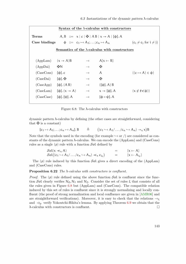
6.3 Instantiations of the dynamic pattern λ-calculus
Syntax of the λ-calculus with constructors
Terms A,B ::= x | c | z | AB | x _ A | |φ|. A
Case bindings φ ::= c1 7→ A1; . . . ; cn 7→ An (ci 6= cj for i 6= j)
Semantics of the λ-calculus with constructors
(AppLam) (x _ A)B → Ax← B
(AppDai) zN → z
(CaseCons) |φ|. c → A ((c 7→ A) ∈ φ)
(CaseDai) |φ|.z → z
(CaseApp) |φ|. (AB) → (|φ|. A)B
(CaseLam) |φ|. (x _ A) → x _ |φ|. A (x 6∈ fv(φ))
(CaseCase) |φ|. |ψ|. A → |φ ψ|. A
Figure 6.8: The λ-calculus with constructors
dynamic pattern λ-calculus by defining (the other cases are straightforward, consideringthat z is a constant)
|c1 7→ A1; . . . ; cn 7→ An|. B ,(
(c1 → A1/ . . . /cn → An) _x x)
B
Note that the symbols used in the encoding (for example → or /) are considered as con-stants of the dynamic pattern λ-calculus. We can encode the (AppLam) and (CaseCons)rules as a single (ρ) rule with a function Sol defined by
Sol(x ≺≺x A) = x← A
Sol(
(c1 → A1/ . . . /cn → An) ≺≺x ci0)
= x← Ai0
The (ρ) rule induced by this function Sol gives a direct encoding of the (AppLam)and (CaseCons) rules.
Proposition 6.22 The λ-calculus with constructors is confluent.
Proof. The (ρ) rule defined using the above function Sol is confluent since the func-tion Sol clearly verifies H0,H1 and H2. Consider the set of rules ξ that consists of allthe rules given in Figure 6.8 but (AppLam) and (CaseCons). The compatible relationinduced by this set of rules is confluent since it is strongly normalizing and locally con-fluent (the proof of strong normalization and local confluence are given in [AMR06] andare straightforward verifications). Moreover, it is easy to check that the relations →ξ
and ⇒ρ verify Yokoutchi-Hikita’s lemma. By applying Theorem 6.9 we obtain that theλ-calculus with constructors is confluent.
143

Chapter 6 Confluence of pattern-based λ-calculi
Conclusion and future works
We propose here a different formulation for different pattern-based calculi and we usethe confluence properties of the general formalism to give alternative confluence proofsfor these calculi. The general confluence proof uses the standard techniques of parallelreduction of Tait and Martin-Lof and Yokouchi-Hikita’s lemma. The method proposedby M. Takahashi [Tak95] gives in general more elegant and shorter proofs by using thenotion of complete developments. Reformulating the hypotheses H0,H1 and H2 andadapting the proofs of this chapter is easy but given a pattern-calculus the reformulatedhypotheses are often more difficult to prove than for the original case.
Moreover, we show that the proof of confluence of the ρ-calculus is easy to deducefrom our general result as soon as the structure operator has no equational theory.Nevertheless, if one wants to switch to non-unitary matching (and this is very useful ispractice [BBK+06, CDE+02]) then the ρ rule should return a collection of results andthe structure operator should be (at least) associative and commutative. This extensionis syntactically and semantically non-trivial and opens new challenging problems. Eventhe extension of the λ-calculus with term collections is not trivial as it is shown in thefollowing chapters.
144

Part III
Categorical semantics of the parallelλ-calculus
145

Chapter 7
Categorical semantics of the λ-calculus
Context The categorical semantics of the untyped λ-calculus, which is based on Carte-sian closed categories (ccc) with reflexive objects [Mac98], provides a rich frameworkto classify all the existing models of the λ-calculus [Bar84]. One of the most strikingproperties of this semantics is that it is complete in a very strong sense [Sco80a, Sco80b]:for each extension T of the basic equational theory of the λ-calculus, it is possible to finda reflexive object such that the equational theory induced by the interpretation of pureλ-terms in this object is exactly the theory T.
Consequently, there exists a reflexive object, in a ‘syntactical’ ccc of partial equivalencerelations, which captures β-conversion, so that two terms having the same denotationin all reflexive objects have the same denotation in this particular object, and thus areβ-convertible.
In other words, we obtain the completeness property by showing that the syntax ofthe λ-calculus has already the structure of a Cartesian closed category with reflexiveobjects, i.e. it is a λ-model.
Contributions This chapter recalls some basic material used in the categorical seman-tics of the λ-calculus and sketches the completeness proof. All the proof details will begiven in Chapter 9 for the case of the parallel λ-calculus.
The reader may found more details on categories in [Mac98, AL91]. Several goodintroductions on the usual interpretation of the simply typed λ-calculus in cccs areavailable, see for example [AC98] or the master course notes of P.-A. Mellies. More onmodels for the untyped λ-calculus can be found in [Sco96, Bar84, AC98, AL91].
Part III of this thesis is a joint work with Alexandre Miquel. The following chaptersare directly inspired from our official [FM07] and non official documents.
Outline of the chapter In Section 7.1 we recall basic definitions related to Cartesianclosed categories and reflexive objects in order to fix the notations used in the following.In Section 7.2 we give the interpretation of the pure λ-terms in a given Cartesian closedcategory and state its soundness. In Section 7.4 we sketch the proof of the completenessproperty for the interpretation of pure λ-terms.
7.1 Cartesian closed categories and reflexive objects
We first recall the definition of a category and of a Cartesian closed category.
147
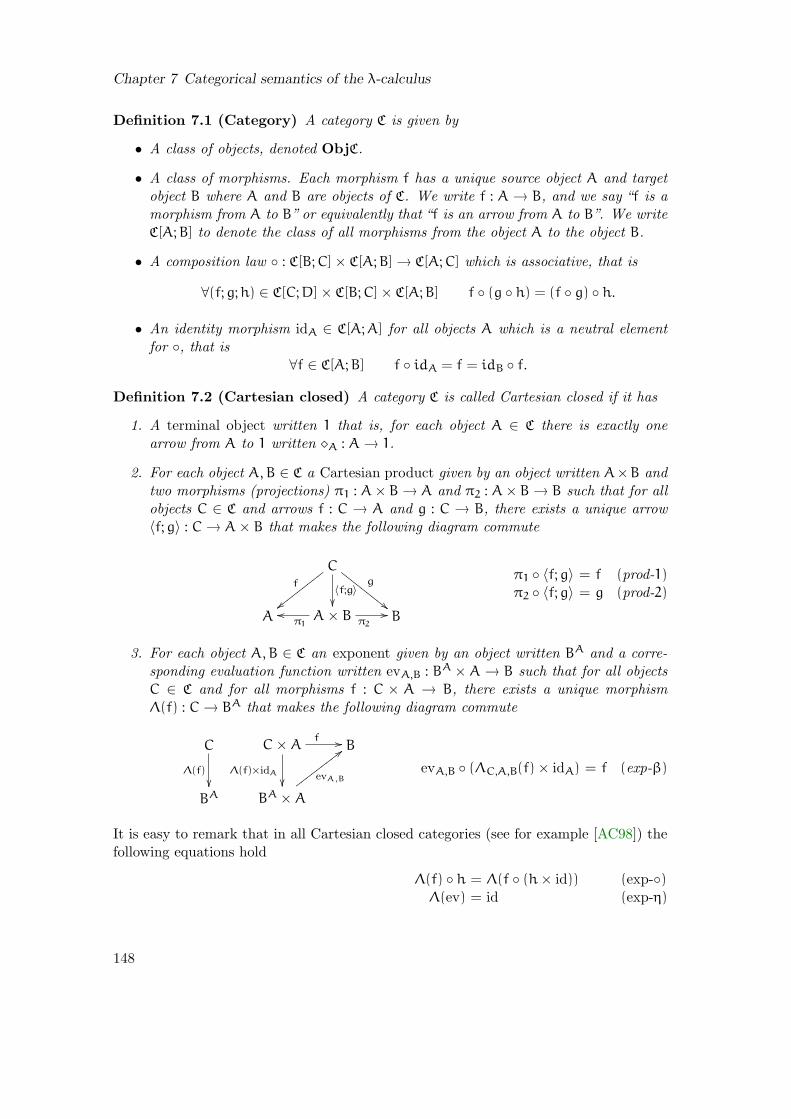
Chapter 7 Categorical semantics of the λ-calculus
Definition 7.1 (Category) A category C is given by
• A class of objects, denoted ObjC.
• A class of morphisms. Each morphism f has a unique source object A and targetobject B where A and B are objects of C. We write f : A → B, and we say “f is amorphism from A to B” or equivalently that “f is an arrow from A to B”. We writeC[A;B] to denote the class of all morphisms from the object A to the object B.
• A composition law : C[B;C] × C[A;B]→ C[A;C] which is associative, that is
∀(f;g;h) ∈ C[C;D] × C[B;C] × C[A;B] f (g h) = (f g) h.
• An identity morphism idA ∈ C[A;A] for all objects A which is a neutral elementfor , that is
∀f ∈ C[A;B] f idA = f = idB f.
Definition 7.2 (Cartesian closed) A category C is called Cartesian closed if it has
1. A terminal object written 1 that is, for each object A ∈ C there is exactly onearrow from A to 1 written ⋄A : A→ 1.
2. For each object A,B ∈ C a Cartesian product given by an object written A×B andtwo morphisms (projections) π1 : A× B→ A and π2 : A× B→ B such that for allobjects C ∈ C and arrows f : C → A and g : C → B, there exists a unique arrow〈f;g〉 : C→ A× B that makes the following diagram commute
Cf
xxxxxxxxx
〈f;g〉
g
""FFFFFFFFF
A A× Bπ1
ooπ2
// B
π1 〈f;g〉 = f (prod-1)π2 〈f;g〉 = g (prod-2)
3. For each object A,B ∈ C an exponent given by an object written BA and a corre-sponding evaluation function written evA,B : BA ×A→ B such that for all objectsC ∈ C and for all morphisms f : C × A → B, there exists a unique morphismΛ(f) : C→ BA that makes the following diagram commute
C
Λ(f)
C×A
Λ(f)×idA
f // B
BA BA ×A
evA,B
;;wwwwwwwwwevA,B (ΛC,A,B(f) × idA) = f (exp-β)
It is easy to remark that in all Cartesian closed categories (see for example [AC98]) thefollowing equations hold
Λ(f) h = Λ(f (h× id)) (exp-)Λ(ev) = id (exp-η)
148

7.2 Interpretation of pure λ-terms
Definition 7.3 (Reflexive object) A reflexive object of a ccc C is a triple (D, lam, app)
formed by an object D ∈ C and two arrows lam : DD→ D and app : D→ DD such thatapp lam = idDD .
7.2 Interpretation of pure λ-terms
The syntax of the λ-calculus used in this chapter was defined in Part I. Terms are denotedhereM,N (instead of A,B) because it fits better with the notations used in the followingchapters. We recall that the syntax of the λ-calculus is defined by
M,N ::= x | λx .M | MN
The corresponding equational theory is given by the equational axiom
(β) (λx .M)N = Mx := N
In this section, we work in a fixed Cartesian closed category C. Let (D, lam, app) bea reflexive object of C. The idea of the interpretation is to consider each pure λ-term asa simply typed λ-term expressed in a degenerate type system with only two ‘types’ Dand DD, plus coercions lam : DD→ D and app : D→ DD relating both types.
In this setting, typing contexts degenerate into (ordered) lists of variables
ℓ ::= [] | ℓ, x
in which variables are implicitly declared with typeD. Each list (context) ℓ is interpretedas an object JℓK of C which is defined by:
J[]K = 1 and Jℓ, xK = JℓK ×D .
To each pair (ℓ, x) formed by a list of variables ℓ and a variable x that belongs to ℓ, wedefine the projection πx
ℓ : JℓK→ D by setting
πxℓ,x = π2 ∈ JℓK ×D→ D
πxℓ,y = πx
ℓ π1 ∈ JℓK ×D→ D (if y 6= x)
Each term M whose free variables belong to a list of variables ℓ is interpreted by anarrow JMKℓ : JℓK→ D which is defined by the equations given in Figure 7.1.
With a little abuse of notations, we write FV (N) ⊂ ℓ to express that all the freevariables of N occur (at least once) in the list ℓ. Notice that a variable x may occurseveral times in a list ℓ, but that the interpretation JMKℓ : JℓK→ D systematically bindsthe last occurrence of x in ℓ. The reader is invited to check that this choice (which isimplemented by the definition of the projections πx
ℓ : JℓK → D) is consistent with theinterpretation of λ-abstractions.
The soundness of this interpretation relies on the following propositions.
149

Chapter 7 Categorical semantics of the λ-calculus
(Var)
(Lam)
(App)
JxKℓ = πxℓ
Jλx .MKℓ = lam Λ(JMKℓ,x)
JMNKℓ = ev 〈app JMKℓ; JNKℓ〉
Figure 7.1: Interpretation of pure λ-terms
Proposition 7.4 (Soundness w.r.t. substitution) Given a list of variables ℓ and avariable x, for all terms M and N such that FV (M) ⊂ (ℓ, x) and FV (N) ⊂ ℓ,we have:
JMx := NKℓ = JMKℓ,x 〈id; JNKℓ〉
Proposition 7.5 (Soundness w.r.t. β-reduction) Given a list of variables ℓ, for allterms M and M ′ whose free variables occur in ℓ we have
M→β M′ ⇒ JMKℓ = JM ′Kℓ
As a corollary, it is clear that β-convertible terms have the same denotation in anyreflexive object of any ccc. Notice that if we want to extend this result to η-conversion,we must assume that lam app = idD too, which means that DD is not only a retractof D, but that DD is actually isomorphic to D.
What is more interesting is that the converse of the soundness property is true: iftwo λ-terms have the same denotation in all reflexive objects of all cccs, then these λ-terms are β-convertible. This property, studied in Section 7.4, is often mentioned as thecompleteness property.
In the following section, we give examples of models of the untyped λ-calculus takenin the category of Scott domains.
7.3 Examples in Scott domains
In this section, we give a smooth presentation of the first historical model of the untypedλ-calculus given by Scott [Sco80a, Sco80b].
A Scott domain is a poset (D,≤) satisfying particular axioms (see below for a precisedefinition). Domain equations such as D ≃ (D → D) have non trivial solutions whenworking with continuous functions.
The following definitions should be read with the following intuitions. Each point of aScott domain D represents some amount of information. The elements of D are orderedby the partiality order: x ≤ y means that x is less defined than y. The least element ⊥denotes thus the lack of observable information, which corresponds in computer scienceto non-termination. The restriction to continuous functions (that makes the thingswork) that is, to functions satisfying the monotonicity as well as the finiteness propertyensure respectively that we cannot extract information from non-termination (the halting
150

7.3 Examples in Scott domains
problem) and that a finite piece of output is only produced by a finite piece of input(commutation with directed limits).
Definition 7.6 (Directed set — cpo) Given a partial order set (D,≤) a non-emptysubset ∆ ⊆ D is called directed if for all x, y ∈ ∆ there exists a z ∈ ∆ such that x ≤ z
and y ≤ z.
A cpo (D,≤) is a partial order with a least element denoted ⊥D and such that eachdirected set ∆ ⊆ D has a least upper bound denoted
∨
∆.
Definition 7.7 (Compact—Algebraic cpo) An element d ∈ D is called compact iffor each directed set ∆ ⊆ D the following implication holds:
d ≤∨
∆⇒ ∃x ∈ ∆ d ≤ x
We write K(D) for the set of all compact elements of D.
A cpo (D,≤) is called algebraic is for all elements x ∈ D the set d ∈ K(D)|d ≤ x isdirected and has least upper bound x.
Definition 7.8 (Scott domain) A Scott domain is an algebraic cpo (D,≤) such thatevery set bounded B ⊆ D has a least upper bound.
Definition 7.9 (Monotonic — Continuous) Let (D,≤) and (D ′,≤ ′) be cpos. Afunction f : D→ D ′ is called monotonic if
∀x, y ∈ D x ≤ y⇒ f(x) ≤ ′ f(y) .
It is continuous if moreover it is finite that is, for all directed subset ∆ of D we have
f(∨
∆) =∨
f(∆)
Theorem 7.10 The category SCOTT of Scott domains and continuous functions is aCartesian closed category with the following structure. For two Scott domains (D,≤D)
and (E,≤E), we define
• the Scott domain (D × E,≤×) where D × E = (x, y) | x ∈ D and y ∈ E and(x, y) ≤ (x ′, y ′) if (x ≤D x
′, y ≤E y′).
• the Scott domain (D ⇒ E,≤⇒) where D ⇒ E is the set of continuous functionsfrom D to E and f ≤⇒ g if for all x ∈ D we have f(x) ≤E g(x).
Theorem 7.11 There exist reflexive objects in the category SCOTT.
The historical reflexive objects are the well-known D∞-models. We refer to [AC98]for their constructions.
151

Chapter 7 Categorical semantics of the λ-calculus
7.4 Completeness
The completeness result mentioned in the section 7.2 is an immediate consequence of amore general result, which says that for each λ-theory T, there is a reflexive object thatcaptures the equational axioms of T exactly.
Definition 7.12 (λ-theory) A λ-theory is an equivalence relation T over the set Λ ofopen λ-terms (taken up to α-conversion) which is closed under the following rules:
(λx .M) =T Mx := N
M =T M′
MN =T M′N
N =T N′
MN =T MN′
M =T M′
λx .M =T λx .M′
As we already mentioned above, any reflexive object (D, lam, app) defines a λ-theorywritten =D and defined as follows
M =DM′ iff JMKD = JM ′KD
for all M,M ′ ∈ Λ. The interesting point is that we can define a ‘syntactic’ category inwhich each λ-theory is represented by a reflexive object. This category is the categorybased on the following notion of λ-per. Let us first recall that a partial equivalencerelation (per) on Λ is a symmetric and transitive relation on Λ.
Definition 7.13 (λ-per) A λ-per is a partial equivalence relation A ⊂ Λ2 such that=β A ⊂ A, that is, such that (M,M ′) ∈ A and M ′ =β M
′′ entail (M,M ′′) ∈ A forall M,M ′,M ′′ ∈ Λ.
Since a per is not required to be reflexive, it is natural to define the domain of a per Aas follows.
Definition 7.14 (Domain) The domain of a per is defined by
dom(A) = M ∈ Λ | (M,M) ∈ A .
Let A be a per, we write M ∈ A when M ∈ dom(A). It is straightforward to checkthat A ⊂ dom(A)2, and that the relation A is but a total equivalence relation on dom(A).Conversely, any equivalence relation defined on a subset of Λ is a per on Λ, which givesan equivalent definition to the notion of per. Moreover, the class of all pers (on Λ) isclosed under arbitrary intersection. The following lemma defines the realisability arrowover λ-pers.
Lemma 7.15 If A and B are pers, then the following binary relation is also a per.
A→ B = (M1,M2) ∈ Λ2 | ∀(N1, N2)∈A (M1N1,M2N2) ∈ B
152

7.4 Completeness
In this framework, a λ-per is but a per which is compatible with the β-conversion equiv-alence relation. As for the class of pers, the class of λ-pers is closed under arbitraryintersection as well as it is closed under the realisability arrow (A,B) 7→ (A → B). Inparticular, the per A→ B is a λ-per as soon as A and B are λ-pers. In what follows, wewill frequently use λ-pers of the form
N→ A = (N,N)→ A
where N is a fixed term and A an arbitray λ-per.
Definition 7.16 The category λPER is defined as follows.
• The objects of λPER are λ-pers.
• Given two λ-PERs A and B, the hom-set λPER[A;B] is defined by
λPER[A;B] = dom(A→ B)/≈A→B
• Identity and composition are defined for all objects A,B,C ∈ λPER and for allarrows M ∈ λPER[B;C] and N ∈ λPER[A;B] by
idA = λx . x ∈ λPER[A;A]
M N = λx .M(Nx) ∈ λPER[A;C]
(taking the corresponding operations on equivalence classes).
We can check that:
Proposition 7.17 The category λPER is a ccc with the following structure.
• A× B = (true→ A) ∩ (false→ B) and 1 = Λ2
• π1 = λp . p true, π2 = λp . p false and 〈M;N〉 = λxp . p (Mx) (Nx)
• BA = A→ B
• ev = λp . (π1p) (π2p) and Λ(M) = λxy .M (λp . pxy).
Noticing that any λ-theory T ⊂ Λ2 is a λ-per of domain Λ, we can easily check that:
Proposition 7.18 (λ-theories as reflexive objects) — For all λ-theories T, the triple(T, λxy . xy, λx . x) is a reflexive object in the category λPER.
Notice that the embedding-retraction pair (lam, app) = (λxy . xy, λx . x) does notdepend on the λ-theory T. Consequently, the denotation JMKT
ℓ of a term M (withFV (M) ⊂ ℓ) does not depend on T too. This denotation is actually characterized bythe following lemma:
153
Chapter 7 Categorical semantics of the λ-calculus
Lemma 7.19 Let T be a λ-theory (that we also consider as a reflexive object of λPER).For all lists of variables ℓ = (x1, . . . , xn) and for all terms M such that FV (M) ⊂ ℓ, onehas
JMKTℓ =β λz .Mx1 := π
x1
ℓ (z); . . . ; xn := πxn
ℓ (z) .
We can now easily conclude that:
Proposition 7.20 Let T be a λ-theory (that we also consider as a reflexive object ofλPER). For all lists of variables ℓ, and for all terms M1 and M2 such that FV (M1) ∪FV (M2) ⊂ ℓ, one has
JM1KTℓ = JM2K
Tℓ iff M1 =T M2 .
Conclusion
In this chapter, we recall the sound and complete categorical semantics for the λ-calculus.In the following chapters, we extend this result to the parallel λ-calculus.
154
Chapter 8
Categorical semantics of the parallelλ-calculus
Context The starting point of this work was the semantical study of the ρ-calculus. AScott semantics revealed the similarity between term collections of the ρ-calculus inter-preted as the binary join and Boudol’s parallel construct of the parallel λ-calculus [Bou94](up to the fact that term collections are not systematically required to be associative,commutative and/or idempotent).
Formally, the parallel λ-calculus is obtained by extending the pure λ-calculus with abinary operator M // N, that intuitively represents the parallel execution of M and N.The parallel λ-calculus adds to the equational theory of the pure λ-calculus the singleequational axiom (δ) expressing the distributivity of function application w.r.t. parallelaggregation.
The parallel λ-calculus was initially introduced as a tool to study full-abstraction ofthe interpretation of λ-terms in Scott domains. In this framework, Boudol extended theinterpretation of pure λ-terms to the parallel construction using the join operation.
Scott semantics is well-suited to achieve full-abstraction but it is not sufficient to cap-ture neither the basic equational theory of the calculus nor many interesting extensionsof it – typically when dealing with extensionality. In the same way, interpreting theparallel operator as the binary join automatically validates associativity, commutativityand idempotence, although on a purely syntactical level, these equations are clearly in-dependent from the basic equations (β) and (δ). For these reasons, there is a need for amore general and more modular semantics.
The semantical study of the ρ-calculus also pointed out many interesting problemsrelated to the interaction between a mechanism of pattern-matching and the parallelconstruct. These problems helped us to grasp the importance of linear terms which playa central role in the proof of completeness (Boudol’s shift towards the λ-calculus withresources [BCL99] seems to be motivated by similar reasons).
Contributions We first give a modular presentation of the parallel λ-calculus: the corecalculus consists of the (β) and the (δ) equational axioms while some extensions are pos-sible including some equational axioms for extensionnality and some equational axiomsexpressing associativity, commutativity and idempotence of the parallel operator. Thisgives 24 variants of the calculus (see below for more details).
We define a sound categorical semantics for the parallel λ-calculus, based on a notion
155

Chapter 8 Categorical semantics of the parallel λ-calculus
of aggregation monad which is modular w.r.t. the 24 equational theories of the calculus.Particular cases of this semantics are given by Boudol’s models.
The given semantics is complete in a very strong sense: for each congruence extendingone of the 24 equational theories of the parallel λ-calculus there exists a reflexive object,adapted to the considered equational theory, such that the equational theory induced bythe interpretation of parallel λ-terms in this object is exactly this congruence.
To prove completeness, we introduce a category of partial equivalence relations adaptedto parallelism, in which any extension of the basic equational theory of the calculus isinduced by some model (see Chapter 9).
We also present abstract methods to construct models of the parallel λ-calculus in cat-egories where particular equations have solutions, such as the category of Scott domainsand its variants (see Chapter 10).
We think that the categorical semantics introduced here will contribute to a betterunderstanding of the interaction between pattern-matching and the parallel construct,and thus will constitute a significant step towards a denotational semantics for the ρ-calculus.
Outline of the chapter In Section 8.1, we present the syntax and equational theory ofthe parallel λ-calculus and define the notion of linear terms. In Section 8.2, we recallsome basic definitions for monads and algebras. In Section 8.3, we introduce and studythe notion of aggregation monads. In Section 8.4, we first give the definition of thecategorical models of the parallel λ-calculus and we then define the interpretation ofparallel λ-terms in this model and we show its soundness. The last section (Section 8.5)gives examples of such models in Scott domains.
8.1 The parallel λ-calculus
We first give a detailed presentation of the syntax and the equational theory of theparallel λ-calculus which is summarized in Figure 8.1 page 158.
8.1.1 The core calculus
The parallel λ-calculus is obtained by extending the pure λ-calculus with a binary oper-ator M//N representing the parallel execution of M and N. Formally, the terms of theparallel λ-calculus are given by
M,N ::= x | λx .M | MN | M// N
and the corresponding equational theory is defined from the two equational axioms
(β)
(δ)
(λx .M)N = Mx := N
(M1 //M2)N = M1N //M2N
In the following, we will consider parallel λ-terms from the point of view of equationalreasoning rather than from the point of view of reduction. However, both equational
156

8.1 The parallel λ-calculus
axioms can also be presented as rewrite rules (orienting them from left to right), and itcan be checked that the rewrite systems induced by β, δ and βδ are confluent.
8.1.2 Extensions of the equational theory
In many situations, it is desirable to extend the core calculus with one of the followingequational axioms:
(ǫ)
(η)
λx . (M1 //M2) = (λx .M1) // (λx .M2)
λx .Mx = M (if x /∈ FV (M))
Again, both equation axioms can be presented as reduction rules, orienting them fromleft to right. Notice that in the presence of equational axiom δ, the equational axiom η
subsumes ǫ, that is: ǫ ⊂ δη (equationally). In fact, we can check that
(λx .M1) // (λx .M2) =η λy .(
(λx .M1) // (λx .M2))
y
=δ λy .(
(λx .M1)y // (λx .M2)y)
=β λy .(
M1x := y //M2x := y)
=α λx . (M1 //M2)
From the point of view of the corresponding rewrite systems, both reduction rules δand η make a critical pair which is closed with the ǫ-reduction rule.
Finally, the parallel λ-calculus can be extended with any combination of the threeequational axioms expressing associativity, commutativity and idempotence of the par-allel operator:
(A)
(C)
(I)
(M1 //M2) //M3 = M1 // (M2 //M3)
M1 //M2 = M2 //M1
M//M = M
In what follows, most definitions will be modularized in order to handle the 24 variantsof the calculus obtained by combining each of the 3 basic calculi βδ, βδǫ and βδη withthe 23 = 8 possible combinations of A, C, and I.
8.1.3 Linearity
Definition 8.1 (Linear term) Let T be an equational theory of the parallel λ-calculuswhich contains at least β and δ. We say that a termM is linear (w.r.t. its first argument)in the theory T when
M(N1 // N2) =T MN1 //MN2
for all terms N1, N2.
By substitutivity, it is equivalent to say that M(x // y) =T Mx //My , where x and yare fresh variables.
When a term M is linear in the theory βδ, we simply say that M is linear. Examplesof linear terms are the identity term λx . x and more generally all the terms of the formλx . x~N where x /∈ FV (~N) (i.e. tuples).
157

Chapter 8 Categorical semantics of the parallel λ-calculus
(β)
(δ)
(ǫ)
(η)
(A)
(C)
(I)
The core calculus
M,N ::= x | λx .M | MN | M// N
(λx .M)N = Mx := N
(M1 //M2)N = M1N //M2N
Extensions of the equational theory
λx . (M1 //M2) = λx .M1 // λx .M2
λx .Mx = M (if x /∈ FV (M))
(M1 //M2) //M3 = M1 // (M2 //M3)
M1 //M2 = M2 //M1
M//M = M
Figure 8.1: The parallel λ-calculus
It is important not to confuse the notion of linearity given here with the more syntacticnotion of linear λ-terms (referred below as syntactic linearity) that says that a λ-term issaid to be linear when all its free and bound variables occur exactly once. In particular,there is no inclusion between both notions:
• The term λx . x(λy . yy) is linear but not syntactically linear,
• The term λxy . yx is syntactically linear but not linear.
8.2 Monads and algebras
We first give the categorical definition of a monad. Then, we give some intuitions comingfrom functional programming monads.
Definition 8.2 (Monad) A monad over a category C is a triple (T, η, µ) formed by anendofunctor T in the category C equipped with two natural transformations η : I → Tand µ : T2→ T such that the following diagrams commute:
T
ηT
Tη //
BBBB
BBBB
BBBB
BBBB
T2
µ
T2
µ// T
T3
µT
Tµ // T2
µ
T2
µ// T
µX TηX = idTX (mon-1)
µX ηTX = idTX (mon-2)
µX TµX = µX µTX (mon-3)
158
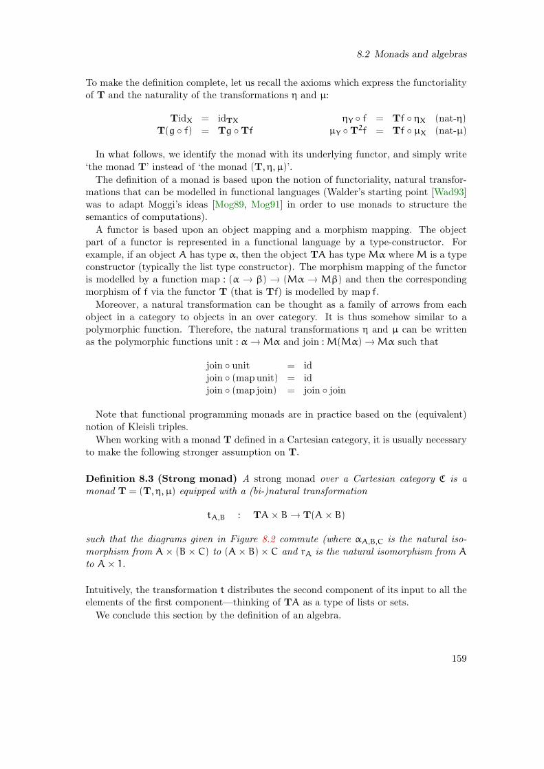
8.2 Monads and algebras
To make the definition complete, let us recall the axioms which express the functorialityof T and the naturality of the transformations η and µ:
TidX = idTX
T(g f) = Tg TfηY f = Tf ηX (nat-η)
µY T2f = Tf µX (nat-µ)
In what follows, we identify the monad with its underlying functor, and simply write‘the monad T’ instead of ‘the monad (T, η, µ)’.
The definition of a monad is based upon the notion of functoriality, natural transfor-mations that can be modelled in functional languages (Walder’s starting point [Wad93]was to adapt Moggi’s ideas [Mog89, Mog91] in order to use monads to structure thesemantics of computations).
A functor is based upon an object mapping and a morphism mapping. The objectpart of a functor is represented in a functional language by a type-constructor. Forexample, if an object A has type α, then the object TA has type Mα where M is a typeconstructor (typically the list type constructor). The morphism mapping of the functoris modelled by a function map : (α → β) → (Mα → Mβ) and then the correspondingmorphism of f via the functor T (that is Tf) is modelled by map f.
Moreover, a natural transformation can be thought as a family of arrows from eachobject in a category to objects in an over category. It is thus somehow similar to apolymorphic function. Therefore, the natural transformations η and µ can be writtenas the polymorphic functions unit : α→Mα and join : M(Mα)→Mα such that
join unit = idjoin (mapunit) = idjoin (map join) = join join
Note that functional programming monads are in practice based on the (equivalent)notion of Kleisli triples.
When working with a monad T defined in a Cartesian category, it is usually necessaryto make the following stronger assumption on T.
Definition 8.3 (Strong monad) A strong monad over a Cartesian category C is amonad T = (T, η, µ) equipped with a (bi-)natural transformation
tA,B : TA× B→ T(A× B)
such that the diagrams given in Figure 8.2 commute (where αA,B,C is the natural iso-morphism from A× (B× C) to (A× B) × C and rA is the natural isomorphism from A
to A× 1.
Intuitively, the transformation t distributes the second component of its input to all theelements of the first component—thinking of TA as a type of lists or sets.
We conclude this section by the definition of an algebra.
159
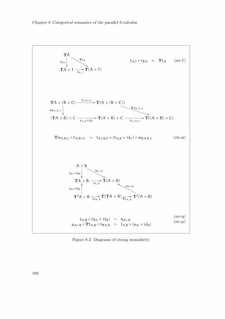
Chapter 8 Categorical semantics of the parallel λ-calculus
TA
rTA
TrA
&&MMMMMMMMMM
TA× 1tA,1
// T(A× 1)
tA,1 rTA = TrA (str-1)
TA× (B× C)tA,B×C //
αTA,B,C
T(A× (B× C))
TαA,B,C
**UUUUUUUUUUUUUUUU
(TA× B) × CtA,B×idC
// T(A× B) × CtA×B,C
// T((A× B) × C)
TαA,B,C tA,B×C = tA×B,C (tA,B × idC) αTA,B,C (str-α)
A× B
ηA×idB
ηA×B
''OOOOOOOOOOO
TA× BtA,B
// T(A× B)
T2A× BtTA,B
//
µA×idB
OO
T(TA× B)TtA,B
// T2(A× B)
µA×B
ggOOOOOOOOOOO
tA,B (ηA × idB) = ηA×B
µA×B TtA,B tTA,B = tA,B (µA × idB)
(str-η)(str-µ)
Figure 8.2: Diagrams of strong monadicity
160
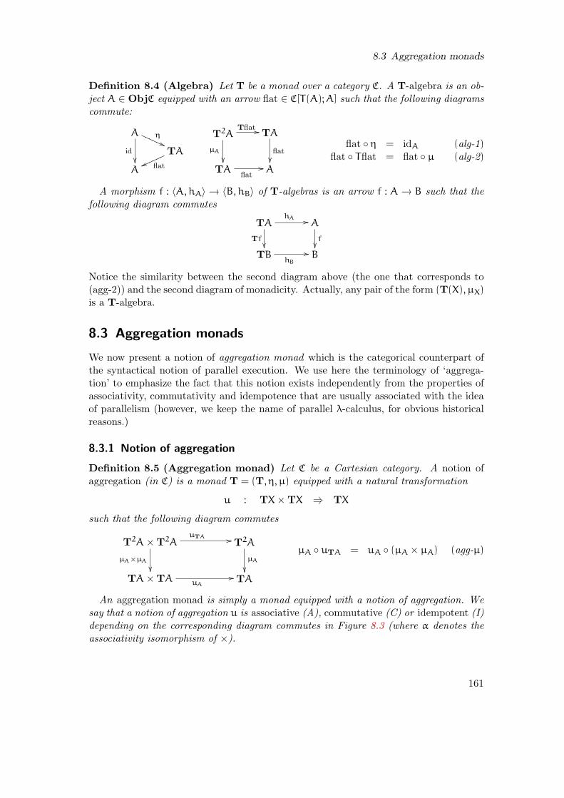
8.3 Aggregation monads
Definition 8.4 (Algebra) Let T be a monad over a category C. A T-algebra is an ob-ject A ∈ ObjC equipped with an arrow flat ∈ C[T(A);A] such that the following diagramscommute:
A
id
η((PPPPPP
TA
flatvvnnnnnn
A
T2A
µA
Tflat // TA
flat
TA
flat// A
flat η = idA (alg-1)
flat Tflat = flat µ (alg-2)
A morphism f : 〈A,hA〉 → 〈B, hB〉 of T-algebras is an arrow f : A → B such that thefollowing diagram commutes
TAhA //
Tf
A
f
TBhB
// B
Notice the similarity between the second diagram above (the one that corresponds to(agg-2)) and the second diagram of monadicity. Actually, any pair of the form (T(X), µX)
is a T-algebra.
8.3 Aggregation monads
We now present a notion of aggregation monad which is the categorical counterpart ofthe syntactical notion of parallel execution. We use here the terminology of ‘aggrega-tion’ to emphasize the fact that this notion exists independently from the properties ofassociativity, commutativity and idempotence that are usually associated with the ideaof parallelism (however, we keep the name of parallel λ-calculus, for obvious historicalreasons.)
8.3.1 Notion of aggregation
Definition 8.5 (Aggregation monad) Let C be a Cartesian category. A notion ofaggregation (in C) is a monad T = (T, η, µ) equipped with a natural transformation
u : TX× TX ⇒ TX
such that the following diagram commutes
T2A× T2AuTA //
µA×µA
T2A
µA
TA× TA uA
// TA
µA uTA = uA (µA × µA) (agg-µ)
An aggregation monad is simply a monad equipped with a notion of aggregation. Wesay that a notion of aggregation u is associative (A), commutative (C) or idempotent (I)depending on the corresponding diagram commutes in Figure 8.3 (where α denotes theassociativity isomorphism of ×).
161

Chapter 8 Categorical semantics of the parallel λ-calculus
Idempotence
TA
〈idA ;idA〉
idA
%%LLLLLLLLLL
TA× TAuA
// TA
uA 〈idA; idA〉 = idA (I-u)
Commutativity
TA× TA uA
))TTTTTTT
〈π2 ;π1〉
TA
TA× TAuA
55jjjjjjj
uA 〈π2;π1〉 = uA (C-u)
Associativity
TA× (TA× TA)
idTA×uA
αTA,TA,TA // (TA× TA) × TA
uA×idTA
TA× TA
uA((PPPPPPPPPPPPP TA× TA
uAvvnnnnnnnnnnnnn
TA
uA (idTA × uA) = uA (uA × idTA) αTA,TA,TA (A-u)
Figure 8.3: ACI diagrams of aggregation
162

8.3 Aggregation monads
The diagram (agg-µ) describes the interaction between the notion of aggregation uand µ. A useful consequence of this diagram is that the arrow uA can always be definedin terms of the arrow uTA. This can also be seen as a description of the interactionbetween u and η.
Lemma 8.6 If (T, u) is a notion of aggregation then the following diagram commutes
TA× TAuA //
ηTA×ηTA
TA
T2A× T2A uTA
// T2A
µA
OOµA uTA (ηTA × ηTA) = uA (agg-η)
Proof. It is easy to check that
µA uTA (ηTA × ηTA) = uA (µA × µA) (ηTA × ηTA) (agg-µ)= uA (mon-2)
8.3.2 Typical examples
Typical notions of aggregation monads are the following.
In the category of sets
• The powerset monad with union (ACI)
• The multiset monad with multi-union (AC)
• The list monad with concatenation (A)
• The free group monad with composition (A)
In the category of Scott domains
• The lower powerdomain monad with join (ACI)
• The upper powerdomain monad with meet (ACI)
In Ab-categories (with finite products), the fundamental aggregation monad is thebinary sum, given as the identity monad equipped with the arrow
π1 + π2 : A×A→ A (ACI)
163

Chapter 8 Categorical semantics of the parallel λ-calculus
8.3.3 Algebras and linear morphisms
Let C be a Cartesian category equipped with an aggregation monad 〈T, u〉.
Definition 8.7 (Aggregation operator) Each T-algebra 〈A,hA〉 can be given an ag-gregation operator pA : A×A→ A defined by
A×AηA×ηA
//pA // A
T(A) × T(A)uA
// T(A)
hA
OOpA = hA uA (ηA × ηA)
The aggregation operator pA inherits the properties of associativity, commutativityand idempotence from the underlying aggregation monad 〈T, u〉 in the sense of thefollowing lemma.
Lemma 8.8 If the aggregation monad 〈T, u〉 is associative, commutative, and/or idem-potent, then for all T-algebras 〈A,hA〉 the aggregation operator pA : A × A → A isassociative, commutative, and/or idempotent in the sense of the following diagrams:
A× (A×A)
id×pA
α // (A×A) ×A
pA×id
A×A
pA %%LLLLLLLL A×A
pAyyrrrrrrrr
AA×A pA
))RRRRRR
〈π2 ;π1〉
A
A×ApA
66llllll
A
〈id;id〉
id
%%LLLLLLLLL
A×A pA
// A
Proof. First, let us suppose that u is idempotent that is, it satisfies (I-u). Then we have:
hA uA (ηA × ηA) 〈idA; idA〉 = hA uA 〈idTA; idTA〉 ηA
= hA idTA ηA (I-u)
= idA (alg-1)
This shows that pA is idempotent.We suppose now that u is commutative that is, it satisfies (C-u). Then we have:
hA uA (ηA × ηA) 〈π2;π1〉 = hA uA 〈π2;π1〉 (ηA × ηA)
= hA uA (ηA × ηA) (C-u)
This shows that pA is commutative.We suppose now that u is associative that is, it satisfies (A-u). The proof of associa-
tivity of pA is given in Figure 8.4. The innermost diagram is the associativity of pA.To show that this diagram commutes we prove the commutativity of the other ones.The outermost diagram is given by (A-u). Diagram (1) is true by the naturality of η.Diagrams (2) and (3) are true by definition of pA for the first component of the product
164

8.3 Aggregation monads
(TA× TA) × TAαTA,TA,TA //
uA×idTA
(2)
TA× (TA× TA)
idTA×uA
(3)(A×A) ×A
(ηA×ηA)×ηA
ffMMMMMMMMMMMMMMMMMαA,A,A //
pA×idA
(1)
A× (A×A)
ηA×(ηA×ηA)
88qqqqqqqqqqqqqqqqq
idA×pA
TA× TA
hA×hA //
uA
%%KKKKKKKKKKKKKKKKKKKKKKKKKKKKKKKKKKKK A×A
pA
""FFF
FFFF
FFFF
FFF
(4)
A×A
pA
||xxxx
xxxx
xxxx
xx
(4)
TA× TA
uA
yyssssssssssssssssssssssssssssssssssss
hA×hAoo
A
TA
hA
OO
Figure 8.4: Associativity of the aggregation operator
165

Chapter 8 Categorical semantics of the parallel λ-calculus
TA× TAuA //
ηTA×ηTA
%%KKKKKKKKKKKKKKKKKKKKKKK
hA×hA
TAhA // A
A×A
ηA×ηA
%%KKKKKKKKKKKKKKKKKKKKKKK(5) T2A× T2A
uA //
ThA×ThA
(6)
(8)
T2A
µA
OO
ThA //
(7)
TA
hA
OO
TA× TA
uA
44hhhhhhhhhhhhhhhhhhhhhhhhhhhhhhhhhhhhhhhhhhhhhh
Figure 8.5: Commutation of the notion of aggregation and the aggregation operator
166

8.3 Aggregation monads
and by (alg-1) for the second one. The proof of diagrams (4) is a bit more elaboratedand is detailed in Figure 8.5. The diagram (5) is given by the naturality of η. Thediagram (6) was proved before and is known as (agg-η). The diagram (7) is given by(alg-2). The diagram (8) is given by the naturality of u.
A consequence of diagram (agg-µ) is that morphisms of algebras are linear in the sensethat they commute with the aggregation operator:
Lemma 8.9 If 〈A,hA〉 and 〈B, hB〉 are T-algebras, then for all morphisms of T-algebrasf : 〈A,hA〉→ 〈B, hB〉 the following diagram commutes
A×ApA //
f×f
A
f
B× B pB
// B
Proof. The proof is given by the following diagram
A×A
(1)
ηA×ηA //
f×f
TA× TAuA //
Tf×Tf
(2)
TAhA //
Tf
(3)
A
f
B× B
ηB×ηB
// TB× TB uB
// TBhB
// B
where the diagram (1) commutes by the naturality of η, the diagram (2) commutes bythe naturality of u and the diagram (3) commutes since f is a morphism of T-algebra.
Remember that for all objects A,B and for all morphisms f : A→ B, the morphism Tfis a morphism of algebras from 〈TA,µA〉 to 〈TB, µB〉.
8.3.4 Strong notion of aggregation
Definition 8.10 (Strong notion of aggregation) A strong notion of aggregation isa notion of aggregation such that the underlying notion of monad is strong and thatsatisfies the following diagram:
(TA× TA) × B〈π1×idB ;π2×idB〉 //
uA×idB
(TA× B) × (TA× B)
tA,B×tA,B
TA× B
tA,B ((QQQQQQQQQQQQQ T(A× B) × T(A× B)
uA×Buukkkkkkkkkkkkkk
T(A× B)
uA×B (tA,B × tA,B) 〈π1 × idB;π2 × idB〉 = tA,B uA × idB (agg-t)
167

Chapter 8 Categorical semantics of the parallel λ-calculus
A strong aggregation monad is simply a strong monad equipped with a strong notionof aggregation.
In particular, all the examples of aggregation monads given in Section 8.3.2 are strongaggregation monads.
8.4 Model of the parallel λ-calculus
8.4.1 Definition
Definition 8.11 (Model of parallel λ-calculus) A model of the parallel λ-calculus isa ccc C equipped with a strong aggregation monad 〈T, u〉 and a quadruple 〈D, lam, app,flat〉such that
• 〈D, lam, app〉 is a reflexive object of C;
• 〈D, flat〉 is a T-algebra;
and such that the following diagram commutes:
(δ)
TD
Tapp
flat // Dapp
T(DD)Λ(flat Tev t)
// DD
where the bottom arrow is built by curryfying the following sequence of morphisms:
T(DD)×Dt
// T(DD×D)Tev
// T(D)flat
// D
Definition 8.12 (ǫ/η/ACI-model) We say that a model of the parallel λ-calculus is
• An ǫ-model when the following diagram commutes:
(ǫ)
TDflat // D
T(DD)
Tlam
OO
Λ(flat Tev t)// DD
lam
OO
• An η-model when lam app = id (η), that is, when the arrows app and lam areconverse isomorphisms;
• Associative (A), commutative (C) or idempotent (I) when the underlying aggrega-tion monad 〈T, u〉 is.
We have seen that in the presence of the equational axiom (δ), the equational axiom(η) subsumes (ǫ), that is ǫ ⊆ δη. The definition of η and ǫ models is sound for thisinclusion in the following sense.
168
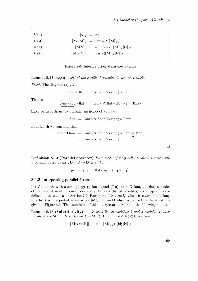
8.4 Model of the parallel λ-calculus
(Var)
(Lam)
(App)
(Par)
JxKℓ = πxℓ
Jλx .MKℓ = lam Λ(JMKℓ,x)
JMNKℓ = ev 〈app JMKℓ; JNKℓ〉
JM// NKℓ = par 〈JMKℓ; JNKℓ〉
Figure 8.6: Interpretation of parallel λ-terms
Lemma 8.13 Any η-model of the parallel λ-calculus is also an ǫ-model.
Proof. The diagram (δ) gives
app flat = Λ(flat Tev t) Tapp
That islam app︸ ︷︷ ︸ flat = lam Λ(flat Tev t) Tapp
Since by hypothesis, we consider an η-model we have
flat = lam Λ(flat Tev t) Tapp
from which we conclude that
flat Tlam = lam Λ(flat Tev t) Tapp Tlam︸ ︷︷ ︸= lam Λ(flat Tev t)
Definition 8.14 (Parallel operator) Each model of the parallel λ-calculus comes witha parallel operator par : D×D→ D given by
par = pD = flat uD (ηD × ηD) .
8.4.2 Interpreting parallel λ-terms
Let C be a ccc with a strong aggregation monad 〈T, u〉, and 〈D, lam, app,flat〉 a modelof the parallel λ-calculus in this category. Context (list of variables) and projections aredefined in the same as in Section 7.2. Each parallel λ-termM whose free variables belongto a list ℓ is interpreted as an arrow JMKℓ : Dℓ → D which is defined by the equationsgiven in Figure 8.6. The soundness of this interpretation relies on the following lemma.
Lemma 8.15 (Substitutivity) — Given a list of variables ℓ and a variable x, thenfor all terms M and N such that FV (M) ⊂ (ℓ, x) and FV (N) ⊂ ℓ, we have:
JMx := NKℓ = JMKℓ,x 〈id; JNKℓ〉
169
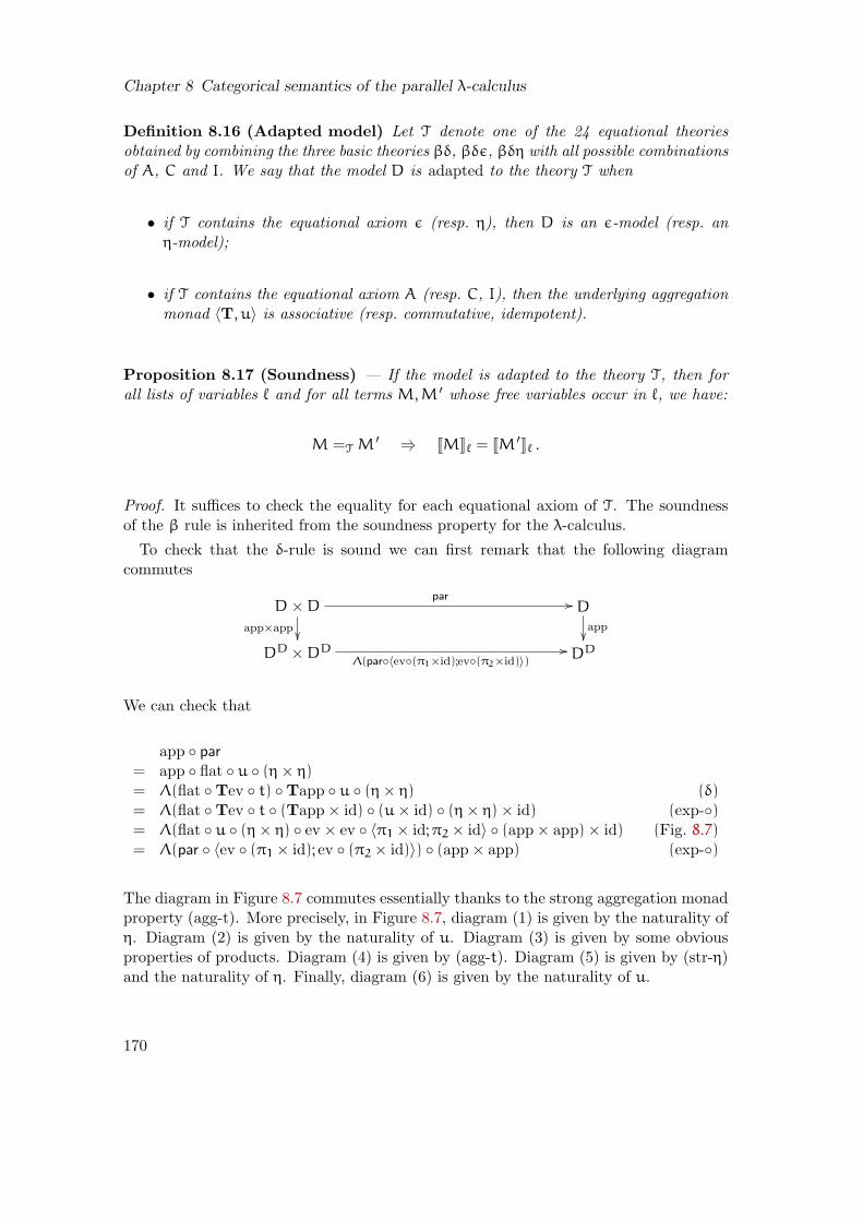
Chapter 8 Categorical semantics of the parallel λ-calculus
Definition 8.16 (Adapted model) Let T denote one of the 24 equational theoriesobtained by combining the three basic theories βδ, βδǫ, βδη with all possible combinationsof A, C and I. We say that the model D is adapted to the theory T when
• if T contains the equational axiom ǫ (resp. η), then D is an ǫ-model (resp. anη-model);
• if T contains the equational axiom A (resp. C, I), then the underlying aggregationmonad 〈T, u〉 is associative (resp. commutative, idempotent).
Proposition 8.17 (Soundness) — If the model is adapted to the theory T, then forall lists of variables ℓ and for all terms M,M ′ whose free variables occur in ℓ, we have:
M =T M′ ⇒ JMKℓ = JM ′Kℓ .
Proof. It suffices to check the equality for each equational axiom of T. The soundnessof the β rule is inherited from the soundness property for the λ-calculus.
To check that the δ-rule is sound we can first remark that the following diagramcommutes
D×D
app×app
par // Dapp
DD ×DDΛ(par〈ev(π1×id);ev(π2×id)〉)
// DD
We can check that
app par= app flat u (η× η)= Λ(flat Tev t) Tapp u (η× η) (δ)
= Λ(flat Tev t (Tapp × id) (u× id) (η× η) × id) (exp-)= Λ(flat u (η× η) ev × ev 〈π1 × id;π2 × id〉 (app × app) × id) (Fig. 8.7)= Λ(par 〈ev (π1 × id); ev (π2 × id)〉) (app × app) (exp-)
The diagram in Figure 8.7 commutes essentially thanks to the strong aggregation monadproperty (agg-t). More precisely, in Figure 8.7, diagram (1) is given by the naturality ofη. Diagram (2) is given by the naturality of u. Diagram (3) is given by some obviousproperties of products. Diagram (4) is given by (agg-t). Diagram (5) is given by (str-η)and the naturality of η. Finally, diagram (6) is given by the naturality of u.
170

8.5 Examples in Scott domains
We now check that
J(M1 //M2)NKℓ
= ev 〈app JM1 parM2K; JNKℓ〉
= ev 〈app par〈JM1Kℓ; JM2Kℓ〉; JNKℓ〉
= ev 〈Λ(par (ev × ev) 〈π1 × id;π2 × id〉︸ ︷︷ ︸f
) (app × app) 〈JM1Kℓ; JM2Kℓ〉; JNKℓ〉
= ev 〈Λ(f) (app × app) π1; π2〉 〈〈JM1Kℓ; JM2Kℓ〉; JNKℓ〉
= ev 〈Λ(f (app × app) × id) π1; π2〉 〈〈JM1Kℓ; JM2Kℓ〉; JNKℓ〉
= par (ev × ev) 〈π1 × id; π2 × id〉 (app × app) × id) 〈〈JM1Kℓ; JM2Kℓ〉; JNKℓ〉
= par 〈ev π1 × id; ev π2 × id〉 (app × app) × id) 〈〈JM1Kℓ; JM2Kℓ〉; JNKℓ〉
= par 〈ev 〈app JM1Kℓ; JNKℓ〉; ev 〈app JM2Kℓ; JNKℓ〉〉
= par 〈JM1NKℓ; JM2NKℓ〉
= JM1N //M2NKℓ
If T contains the ǫ rule, then the soundness of the (ǫ) equational axiom is proved inthe same way as for the soundness of the δ-rule: we check that the following diagramcommutes
D×Dpar // D
DD ×DD
lam×lam
OO
Λ(par〈ev(π1×id);ev(π2×id)〉)// DD
lam
OO
Suppose that T contains the equational axiom (A) respectively the equational ax-iom (C) respectively the equational axiom (I). All models adapted to T validates theseequations by Lemma 8.8.
8.5 Examples in Scott domains
In the category of Scott domains [Sco82, AC98], the ACI-aggregation monad 〈Pl; ∨〉(where Pl denotes the lower powerdomain [Plo76, Smy78]) is the source of a plethora ofmodels for the parallel λ-calculus, due to the fact that:
Proposition 8.18 — Any Scott domain D with a top element is a Pl-algebra whoseaggregation operator pD is the binary join: pD(x, y) = x∨ y (for all x, y ∈ D).
Proof. Remember that a Scott domain has a top element iff it has all its joins (theconverse already holds for cpos). We define the morphism hD : Pl(D) → D from themap
h0 : K(Pl(D)) = P+fin(K(D)) → D
k1; . . . ;kn 7→ k1 ∨ · · · ∨ kn
171

Chapter 8 Categorical semantics of the parallel λ-calculus
(D×D) ×D
(app×app)×id
''NNNNNNNNNNNNNNNNNNNNNN
(η×η)×id
yyttttttttttttttttttt
(1)(TD× TD) × TD
(Tapp×Tapp)×id
$$JJJJJJJJJJJJJJJJJJJ
u×id
~~~~~~
~~~~
~~~~
~~~~
(2)
(DD ×DD) ×D
〈π1×id;π2×id〉
''OOOOOOOOOOOOOOOOOOOOOO
(η×η)×id
wwpppppppppppppppppppppp
(3)TD×D
Tapp×id
@@@
@@@@
@@@@
@@@@
@ T(DD) × T(DD) ×D
〈π1×id;π2×id〉
''NNNNNNNNNNNNNNNNNNNNNN
u×id
zzttttttttttttttttttt
(4)
(DD ×D) × (DD ×D)
(η×id)×(η×id)
wwoooooooooooooooooooooo
ev×ev
T(DD) ×D
t
$$JJJJJJJJJJJJJJJJJJJ
(T(DD) ×D) × (T(DD) ×D)
t×t
(5)
T(DD ×D)
Tev
(6)
T(DD ×D) × T(DD ×D)
Tev×Tev
uoo D×D
η×η
wwoooooooooooooooooooooooo
T(D) TD× TDuoo
Figure 8.7: Soundness of the (δ) rule
172
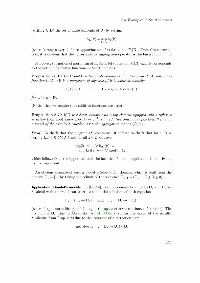
8.5 Examples in Scott domains
(writing K(D) the set of finite elements of D) by setting
hD(x) = supk≪x
h0(k)
(where k ranges over all finite approximants of x) for all x ∈ Pl(D). From this construc-tion, it is obvious that the corresponding aggregation operator is the binary join.
Moreover, the notion of morphism of algebras (cf subsection 8.3.3) exactly correspondsto the notion of additive functions in Scott domains:
Proposition 8.19 Let D and E be two Scott domains with a top element. A continuousfunction f : D→ E is a morphism of algebras iff it is additive, namely:
f(⊥) = ⊥ and f(x∨ y) = f(x) ∨ f(y)
for all x, y ∈ D.
(Notice that we require that additive functions are strict.)
Proposition 8.20 If D is a Scott domain with a top element equipped with a reflexivestructure (lam, app) where app : D→ DD is an additive continuous function, then D isa model of the parallel λ-calculus w.r.t. the aggregation monad 〈Pl; ∨〉.
Proof. To check that the diagram (δ) commutes, it suffices to check that for all k =
k1; . . . ;kn ∈ K(Pl(D)) and for all x ∈ D we have
app(k1 ∨ · · · ∨ kn)(x) =
app(k1)(x) ∨ · · · ∨ app(kn)(x) ,
which follows from the hypothesis and the fact that function application is additive onits first argument.
An obvious example of such a model is Scott’s D∞ domain, which is built from thedomain D0 = ⊤⊥ by taking the colimit of the sequence Di+1 = (Di→ Di) (i ≥ 0).
Application: Boudol’s models In [Bou94], Boudol presents two models D∗ and Ds forλ-calculi with a parallel construct, as the initial solutions of both equations
D∗ = (D∗ → D∗)⊥ and Ds = (Ds →⊥ Ds)⊥
(where ( )⊥ denotes lifting and ( →⊥ ) the space of strict continuous functions). Thefirst model D∗ (due to Abramsky [Abr91, AO93]) is clearly a model of the parallelλ-calculus from Prop. 8.20 due to the existence of a retraction pair
(up∗,down∗) : (D∗ → D∗) ⊳ D∗
173

Chapter 8 Categorical semantics of the parallel λ-calculus
whose second component (the projection) is additive. The second model Ds (whichinterprets a λ-calculus with call-by-value abstractions) can be decomposed as follows
Ds = Vs⊥
Vs = Vs⊥ →⊥ Ds = Vs → Ds
where Vs is a space of values (as opposed to Ds, which is a space of computations). Here,the space of values Vs is again a model of the parallel λ-calculus from Prop. 8.20 due tothe existence of a retraction pair
(λf .ups f, λf .downs f) : (Vs → Vs) ⊳ Vs
whose second component is additive. (Here, (ups,downs) denotes the retraction Vs ⊳ Ds.)
Conclusion
In this chapter, we define a categorical semantics for the parallel λ-calculus and we proveit sound. We prove in the following chapter its completeness.
174

Chapter 9
Completeness by syntactical models
Contributions For each of the 24 equational theories T0 of the parallel λ-calculus ob-tained by combining each of the 3 basic calculi βδ, βδǫ and βδη with the 8 combinationsof A, C and I, we prove the following completeness result: for every congruence T thatcontains T0 there exists a model adapted to T0 such that the equational theory inducedby the interpretation of parallel terms in this object is exactly T.
The proof is based on an adequate notion of pers models as for the proof of com-pleteness of the categorical semantics of the λ-calculus given in Chapter 7. The maindifficulty here is to find a suitable aggregation monad. This is achieved by introducinga boxing monad that ensures that in the per models we only have parallel aggregationof linear terms (in the sense of definition 8.1).
Outline of the chapter In Section 9.1, we extend the notion of λ-per by defining ageneral notion of T-per w.r.t. the equational theories of the parallel λ-calculus. Wedefine and study in Section 9.2 the corresponding category and in Section 9.3 the corre-sponding aggregation monad. The last section (9.4) is devoted to the detailed proof ofthe completeness result.
9.1 The notion of T-per
Let T be one of the 24 equational theories of the parallel λ-calculus mentioned in Sec-tion 8.1 and obtained by combining each of the 3 basic calculi βδ, βδǫ and βδη withthe combinations of A, C and I.
Definition 9.1 (T-per) — A T-partial equivalence relation (T-per) is a partial equiv-alence relation (per) A on the set of parallel λ-terms such that T A ⊂ A, that is, asymmetric and transitive relation A such that
(M,M ′) ∈ A and M ′ =T M′′ ⇒ (M,M ′′) ∈ A
for all terms M,M ′,M ′′.
Definition 9.2 (Domain) The domain of a T-per A is defined by
dom(A) = M | (M,M) ∈ A .
175

Chapter 9 Completeness by syntactical models
T-pers are naturally ordered by inclusion: the smallest T-per is the empty per (ofdomain the empty set) and the largest T-per is the full per (of domain the set of all terms).Moreover, T-pers are closed under arbitrary intersection, and thus form a completedistributive lattice.
Two important constructions of T-pers are the arrow A → B of two T-pers A and Band the parallel closure A+ of one T-per defined as follows.
Definition 9.3 (Arrow T-pers) The arrow A → B of two T-pers A and B is definedfor all M,M ′ by
(M,M ′) ∈ (A→ B) iff ∀N,N ′ ((N,N ′) ∈ A⇒ (MN,M ′N ′) ∈ B)
The arrow construction of pers is a construction which is antimonotonic w.r.t. A andmonotonic w.r.t. B.
Definition 9.4 (Parallel closure) The parallel closure A+ of a T-per A is inductivelydefined by the two following rules
(M,M ′) ∈ A
(M,M ′) ∈ A+
(M1,M′1) ∈ A
+
(M2,M′2) ∈ A
+
M =T M1 //M2
M ′ =T M′1 //M
′2
(M,M ′) ∈ A+
We first show that the two definitions are sound. Note that in the proof of soundness ofthe arrow construction, we use the fact that both A and B are T-pers.
Lemma 9.5 Let A and B be two T-pers. The arrow A→ B is also a T-per.
Proof. We first prove the symmetry of the relation A→ B. Suppose that we have
(M,M ′) ∈ A→ B.
Let (N ′, N) ∈ A. By the symmetry of A, we have (N,N ′) ∈ A and then
(MN,M ′N ′) ∈ B.
By the symmetry of B, we get
(M ′N ′,MN) ∈ B.
We then show the transitivity of the relation A→ B. Suppose that we have
(M,M ′) ∈ A→ B and (M ′,M ′′) ∈ A→ B.
Let (N,N ′) ∈ A. Then we have N ∈ dom(A) and thus (MN,M ′N) ∈ B. But we havealso
(M ′N,M ′′N ′) ∈ B.
The transitivity of B concludes the proof.
176
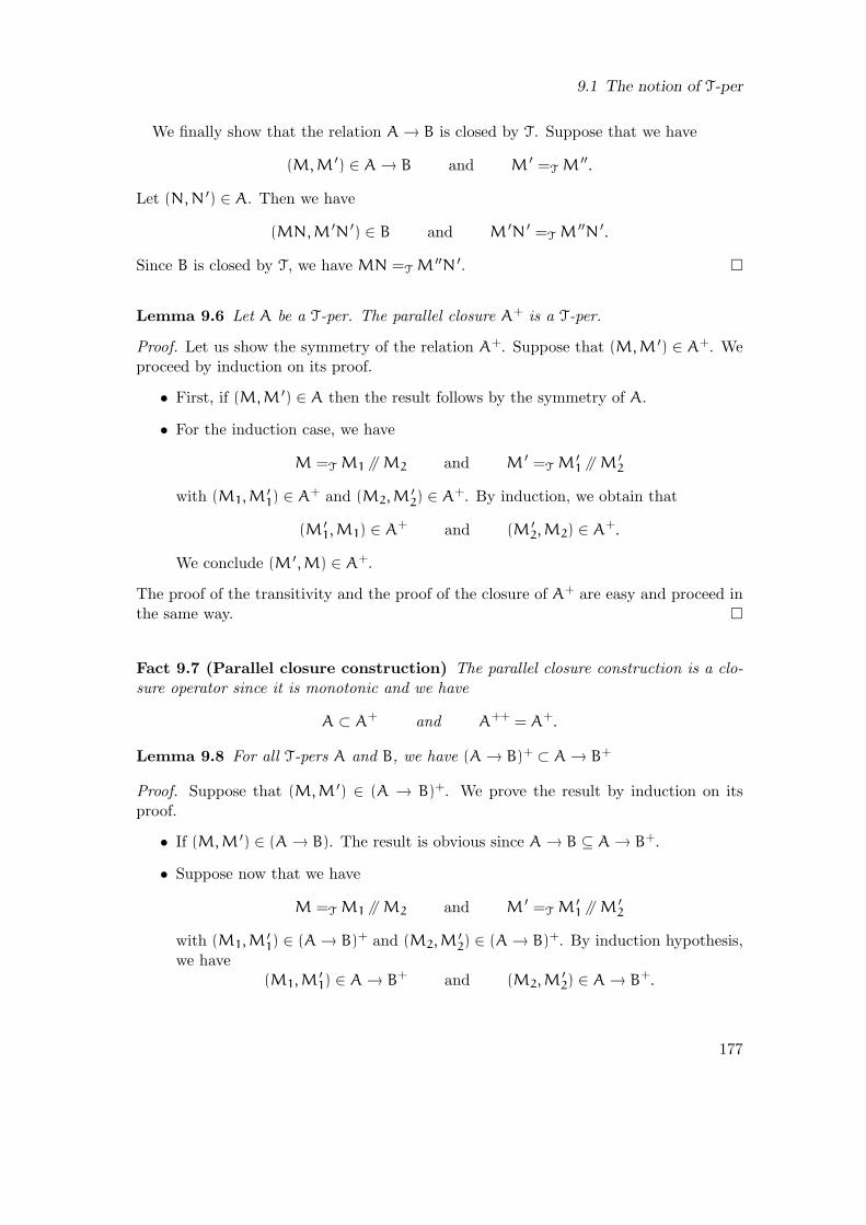
9.1 The notion of T-per
We finally show that the relation A→ B is closed by T. Suppose that we have
(M,M ′) ∈ A→ B and M ′ =T M′′.
Let (N,N ′) ∈ A. Then we have
(MN,M ′N ′) ∈ B and M ′N ′ =T M′′N ′.
Since B is closed by T, we have MN =T M′′N ′.
Lemma 9.6 Let A be a T-per. The parallel closure A+ is a T-per.
Proof. Let us show the symmetry of the relation A+. Suppose that (M,M ′) ∈ A+. Weproceed by induction on its proof.
• First, if (M,M ′) ∈ A then the result follows by the symmetry of A.
• For the induction case, we have
M =T M1 //M2 and M ′ =T M′1 //M
′2
with (M1,M′1) ∈ A
+ and (M2,M′2) ∈ A
+. By induction, we obtain that
(M ′1,M1) ∈ A
+ and (M ′2,M2) ∈ A
+.
We conclude (M ′,M) ∈ A+.
The proof of the transitivity and the proof of the closure of A+ are easy and proceed inthe same way.
Fact 9.7 (Parallel closure construction) The parallel closure construction is a clo-sure operator since it is monotonic and we have
A ⊂ A+ and A++ = A+.
Lemma 9.8 For all T-pers A and B, we have (A→ B)+ ⊂ A→ B+
Proof. Suppose that (M,M ′) ∈ (A → B)+. We prove the result by induction on itsproof.
• If (M,M ′) ∈ (A→ B). The result is obvious since A→ B ⊆ A→ B+.
• Suppose now that we have
M =T M1 //M2 and M ′ =T M′1 //M
′2
with (M1,M′1) ∈ (A→ B)+ and (M2,M
′2) ∈ (A→ B)+. By induction hypothesis,
we have(M1,M
′1) ∈ A→ B+ and (M2,M
′2) ∈ A→ B+.
177
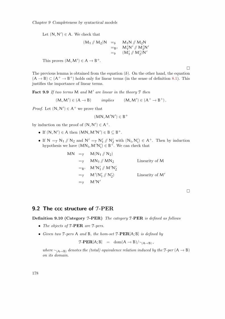
Chapter 9 Completeness by syntactical models
Let (N,N ′) ∈ A. We check that
(M1 //M2)N =δ M1N //M2N
=B+ M ′1N
′ //M ′2N
′
=δ (M ′1 //M
′2)N
′
This proves (M,M ′) ∈ A→ B+.
The previous lemma is obtained from the equation (δ). On the other hand, the equation(A→ B) ⊂ (A+→ B+) holds only for linear terms (in the sense of definition 8.1). Thisjustifies the importance of linear terms.
Fact 9.9 If two terms M and M ′ are linear in the theory T then
(M,M ′) ∈ (A→ B) implies (M,M ′) ∈ (A+→ B+) .
Proof. Let (N,N ′) ∈ A+ we prove that
(MN,M ′N ′) ∈ B+
by induction on the proof of (N,N ′) ∈ A+.
• If (N,N ′) ∈ A then (MN,M ′N ′) ∈ B ⊆ B+.
• If N =T N1 // N2 and N ′ =T N′1 // N
′2 with (Ni, N
′i) ∈ A+. Then by induction
hypothesis we have (MNi,M′N ′
i) ∈ B+. We can check that
MN =T M(N1 // N2)
=T MN1 //MN2 Linearity of M
=B+ M ′N ′1 //M
′N ′2
=T M ′(N ′1 // N
′2) Linearity of M ′
=T M ′N ′
9.2 The ccc structure of T-PER
Definition 9.10 (Category T-PER) The category T-PER is defined as follows
• The objects of T-PER are T-pers.
• Given two T-pers A and B, the hom-set T-PER[A;B] is defined by
T-PER[A;B] = dom(A→ B)/∼(A→B) ,
where ∼(A→B) denotes the (total) equivalence relation induced by the T-per (A→ B)
on its domain.
178
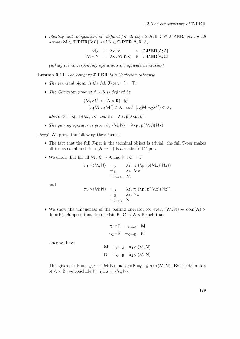
9.2 The ccc structure of T-PER
• Identity and composition are defined for all objects A,B,C ∈ T-PER and for allarrows M ∈ T-PER[B;C] and N ∈ T-PER[A;B] by
idA = λx . x ∈ T-PER[A;A]
M N = λx .M(Nx) ∈ T-PER[A;C]
(taking the corresponding operations on equivalence classes).
Lemma 9.11 The category T-PER is a Cartesian category:
• The terminal object is the full T-per: 1 = ⊤.
• The Cartesian product A× B is defined by
(M,M ′) ∈ (A× B) iff
(π1M,π1M′) ∈ A and (π2M,π2M
′) ∈ B ,
where π1 = λp . p(λxy . x) and π2 = λp . p(λxy . y).
• The pairing operator is given by 〈M;N〉 = λxp . p(Mx)(Nx).
Proof. We prove the following three items.
• The fact that the full T-per is the terminal object is trivial: the full T-per makesall terms equal and then (A→ ⊤) is also the full T-per.
• We check that for all M : C→ A and N : C→ B
π1 〈M;N〉 =β λz . π1(λp . p(Mz)(Nz))
=β λz .Mz
=C→A M
andπ2 〈M;N〉 =β λz . π2(λp . p(Mz)(Nz))
=β λz .Nz
=C→B N
• We show the uniqueness of the pairing operator for every (M,N) ∈ dom(A) ×dom(B). Suppose that there exists P : C→ A× B such that
π1 P =C→A M
π2 P =C→B N
since we haveM =C→A π1 〈M;N〉
N =C→B π2 〈M;N〉
This gives π1P =C→A π1〈M;N〉 and π2P =C→B π2〈M;N〉. By the definitionof A× B, we conclude P =C→A×B 〈M;N〉.
179

Chapter 9 Completeness by syntactical models
Lemma 9.12 In the category T-PER, for every pairs of objets A,B there exists anexponent:
• The exponent is given by BA = (A→ B).
• The evaluation map is given by ev = λp . (π1p) (π2p).
• The currying operator is given by Λ(M) = λxy .M(λp . pxy).
Proof. We prove the following items.
• Let M ∈ C×A→ B. We check that
ev (Λ(M) × id) =β λz . ev(
〈Λ(M)(π1z); π2z〉)
=β λz .Λ(M)(π1z)(π2z)
=β λz .M(λp . p(π1z)(π2z))
=C×A→B M
• Suppose given M ∈ C × A → B. We now prove the uniqueness of the curryingoperator. Suppose given a term M ′ : C→ A→ B such that
ev (M ′ × id) =C×A→B M
We want to showM ′ =C→A→B Λ(M).
Let (N1, N′1) ∈ C and (N2, N
′2) ∈ A. We want to show that
M ′N1N2 =C Λ(M)N ′1N
′2
or equivalently:M ′N1N2 =B Mλp . pN ′
1N′2
But since ev (M ′× id) =C×A→B M and λp . pN1N2 =C×A λp . pN ′1N
′2 we have
(ev (M ′ × id)) (λp . pN1N2) =B M(λp . pN ′1N
′2)
The equality (ev (M ′ × id)) (λp . pN1N2) =β M′N1N2 concludes the proof.
From the two previous results, we conclude the following proposition.
Proposition 9.13 (Ccc of T-PER) The category of T-PER can be given the structureof a ccc.
180

9.3 The aggregation monad of T-PER
9.3 The aggregation monad of T-PER
It would be tempting to define the aggregation monad T of T-PER by setting TA = A+.Unfortunately, the parallel closure operator A 7→ A+ is not functorial (since A ⊂ A+ but(A→ B) 6⊆ (A+→ B+)) and thus cannot be given the structure of a monad. To achievefunctoriality, we first need to introduce the following boxing mechanism that constructsonly linear terms (see Lemma 9.20).
9.3.1 The boxing monad
Definition 9.14 (Boxing terms) For all terms M, we set
[M] = λx . xM
where x is a fresh variable.
This construction can be understood as a 1-uple. Unboxing is performed by applyingI = λx . x, since [M]I =β M.
Definition 9.15 (Boxing T-pers) To each T-per A, we associate a T-per [A] definedby
(M,M ′) ∈ [A] iff
∃(M0,M′0)∈A (M =T [M0] ∧ M ′ =T [M ′
0]) .
This definition is clearly sound and we have
Lemma 9.16 Both T-pers [A] and A are isomorphic via the converse isomorphisms
box = λx . [x] ∈ dom(A→ [A]) and unbox = λx . xI ∈ dom([A]→ A) .
Proof. As remarked above, we have unbox box =A→A I. We prove the other direction.Suppose that we have (N,N ′) ∈ [A] that is,
N =T [N0] and N ′ =T [N ′0] and (N0, N
′0) ∈ A
We check that(box unbox)(N) =β [NI]
=T [[N0]I]
=β [N0]
=[A] [N ′0]
=T N ′
Moreover, the following implication holds.
Lemma 9.17 For all T-pers A and B, we have [A→ B] ⊂ [A]→ B.
181

Chapter 9 Completeness by syntactical models
Proof. Suppose that (M,M ′) ∈ [A→ B] that is
M =T [M0] and M ′ =T [M ′0] and (M0,M
′0) ∈ A→ B
Let (N,N ′) ∈ [A], that is
N =T [N0] and N ′ =T [N ′0] and (N0, N
′0) ∈ A
We check thatMN =T [M0][N0]
=β [N0]M0
=β M0N0
=B M ′0N
′0
=β [M ′0][N
′0]
Definition 9.18 (Boxing functor) The boxing functor is defined as follows
• The object function: A 7→ [A].
• The arrow function: ↑M = [λz . [Mz]] for all M.
The definition is sound since M ∈ dom(A→ B) implies
↑M ∈ dom([A→ [B]]) ⊂ dom([A]→ [B]) .
It actually defines a functor since
• it preserves identity:↑id =[A]→[A] [λz . [z]]
=[A]→[A] λz . z
• it preserves composition:
↑(f g) =β [λy . [f(gz)]]
=[A]→[A] λz . z(λx . [gx])(λy . [fy])
= ↑f ↑g
Lemma 9.19 (Boxing monad) The boxing functor can be given the structure of monadby setting:
– Unit: η = box.
– Multiplication: µ = unbox.
182

9.3 The aggregation monad of T-PER
Proof. Note that all the terms involved in this proof are linear (except in the naturalityof η). This will be used in the section related to the aggregation monad. The twotransformations η and µ are well-defined and define a monad. We show that there arenatural transformations.
• We check that η is natural:
η M =β λz . [Mz]
=β λz . [z](λy . [My])
=β ↑M η
• We check that µ is natural. We first check that
↑M µ =β λz . zI(λx . [Mx])
µ ↑↑M =β λz . z(λx . [x(λy . [My])])I .
Let (N,N ′) ∈ [[A]] that is N =T [[N0]] and N ′ =T [[N ′0]] with (N0, N
′0) ∈ A we
check that(↑M µ)(N) =T ([[N0]]I)(λy . [My])
=β [MN0]
=[B] [MN ′0]
=β [[N ′0](λx . [Mx])]I
=T [[N ′0]](λy . [y(λx . [Mx]]))I
= (µ ↑↑M)(N ′)
• We check that (mon-1) is satisfied. We have
µ ↑η = λz . z(λx . [ηx])I
Let (N,N ′) ∈ [A] this means that N =T [N0] and N ′ =T [N ′0] with (N0, N
′0) ∈ A.
We have(µ ↑η)(N) =T [N0](λx . [[x]])I
=β [[N0]]I
=β [N0]
=[A] [N ′0]
=T N ′
• We check that (mon-2) is satisfied: this is true since η and µ are isomorphic.
• We check that (mon-3) is satisfied. We have
µ ↑µ =β λz . z(λx . [xI])I
µ µ =β λz . (zI)I
183

Chapter 9 Completeness by syntactical models
Let (N,N ′) ∈ [[[A]]] this means that we have N =T [[N0]] and N ′ =T [[N ′0]] with
(N0, N′0) ∈ [A]. We have
(µ µ)(N) =T [[N0]]II
=β N0
=[A] N ′0
=β [[N ′0]I]I
=β [[N ′0]](λx . [xI])I
=β (µ ↑µ)(N ′)
The main property of the boxing mechanism is that boxed objects (including liftedmorphisms ↑M) are linear w.r.t. their first argument, in the sense that
Lemma 9.20 For all M ∈ [A] and for all terms N1, N2,
M(N1 // N2) =T MN1 //MN2
Proof. Let M ∈ [A] that is M =T [M ′0] with M ′
0 ∈ A. We check that
M(N1 // N2) =T [M0](N1 // N2)
=β (N1 // N2)M0
=δ N1M0 // N2M0
=β [M0]N1 // [M0]N2
=T MN1 //MN2
This property is crucial for the definition of the aggregation monad below.
9.3.2 The aggregation monad
Definition 9.21 (Aggregation monad) The aggregation monad T is defined by
• The object function: A 7→ [A]+.
• The arrow function: ↑M = [λz . [Mz]] for all M.
• Unit: η = box.
• Multiplication: µ = unbox.
• Aggregation: u = λp . (π1p) // (π2p).
• Strength: t = λx . (π1x)(λy . [〈y;π2x〉)].
184

9.3 The aggregation monad of T-PER
Of course, one has to check that these constructions fit in their new types, using theproperty of linearity mentioned above.
Lemma 9.22 The functor T is well-defined and is a monad.
Proof. We first show that T fits in its types: If M ∈ A→ B then T(M) ∈ [A]+→ [B]+.
Let M ∈ A→ B and let N ∈ [A]+. We prove that
T(M)(N) ∈ [B]+
by induction on the proof of N ∈ [A]+. Note that since T(M) is linear, it is sufficient tocheck the basic case. So let N ∈ [A]. We have T(M)(N) ∈ [B]. Since
[B] ⊆ [B]+ ,
then we conclude T(M)(N) ∈ [B]+. This concludes the proof.To show that T defines actually a functor and that we have indeed define a monadic
structure, it is sufficient to remark that all terms that are involved in the proof ofLemma 9.19 are linear (except in the naturality of η but it is trivial).
Lemma 9.23 〈T, u〉 is an aggregation monad on the category T-PER.
Proof. We can check that:
µ u =β λz . (π1z // π2z)I=δ λz . (π1z)I // (π2z)I=β u (µ× µ)
Proposition 9.24 〈T, u〉 is a strong aggregation monad on the category T-PER.
Proof. We check that the diagram (agg-t) commutes:
t (u× id) =β λz . ((π1π1z) // (π2π1z))λx . [〈x;π2z〉]=δ λz . (π1π1z)(λx . [〈x;π2z〉]) // (π2π1z)(λx . [〈x;π2z〉])=β λz . t〈π1π1z;π2z〉 // t〈π2π1z;π2z〉=β u (t× t) 〈π1 × id;π2 × id〉
Moreover, it is straightforward to check that the aggregation monad 〈T, u〉 is associative,commutative or idempotent as soon as T contains the corresponding equation.
Lemma 9.25 If T contains the equation A, then the category of T-PER can be equippedwith a strong notion of aggregation that is associative.
185

Chapter 9 Completeness by syntactical models
Proof. We check that
u (u× id) α =β λz .(
π1(z) // π1(π2(z)))
// π2(π2(z))
=A λz . π1(z) //(
π1(π2(z)) // π2(π2(z)))
=β u (id× u)
Lemma 9.26 If T contains the equation C, then the category of T-PER can be equippedwith a strong notion of aggregation that is commutative.
Proof. We check that
u 〈π2;π1〉 =β λz . (π2(z) // π1(z))
=C λz . (π1(z) // π2(z))
= u
Lemma 9.27 If T contains the equation I, then the category of T-PER can be equippedwith a strong notion of aggregation that is idempotent.
Proof. We check thatu 〈id; id〉 =β λz . u(〈z, z〉)
=β λz . (z // z)
=I λz . z
9.4 Completeness
Every model D of the parallel λ-calculus induces a congruence written =D over the setof parallel λ-terms, which is defined for all terms M and M ′ by
M =DM′ iff JMKD
ℓ = JM ′KDℓ
(where ℓ is such that FV (MM ′) ⊂ ℓ). Of course, since the semantics is sound thecongruence =D contains βδ.
We want to show that the converse holds, in the sense that for every congruence T
containing βδ, there exists a model D of the parallel λ-calculus that induces the congru-ence T exactly, namely, there exists a model D such that M =DM
′ iff M =T M′ for all
terms M and M ′.
Theorem 9.28 (Completeness) — Let T0 be one of the 24 equational theories of theparallel λ-calculus mentioned in Section 8.1. For every congruence T ⊇ T0, there existsa T0-per D such that:
186

9.4 Completeness
1. D is a model of the parallel λ-calculus in T0-PER, which is adapted to the the-ory T0;
2. M =DM′ iff M =T M
′ (for all terms M,M ′)
9.4.1 Proof sketch
The theorem is proved as follows. Consider a congruence T ⊇ T0(⊇ βδ). We first noticethat as a binary relation, the congruence T is a T0-per whose domain is the set of allparallel λ-terms. We choose for the object D of Theorem 9.28
D = T
and we show that
1. D is a model in T0-PER, which is adapted to the theory T0. We firstcheck that the model fulfills all the expected properties namely it is a reflexiveobject (Lemma 9.29) and an algebra (Lemma 9.30) and that the diagram (δ) holds(Lemma 9.31). We check (Lemma 9.32 resp. Lemma 9.33) that the model D de-fined above is an ǫ-model (resp. an η-model) as soon as the equational theory T0
contains the equation ǫ (resp. the equation η). Moreover, we know (previous sec-tion) that the underlying aggregation monad that comes with the category T0-PERis associative, commutative, idempotent as soon as T0 contains the correspondingequation.
2. M =DM′ iff M =T M
′ for all terms M and M ′. This is done in Section 9.4.6.
9.4.2 Reflexivity
Lemma 9.29 The reflexive structure for the congruence T is given by
app = λx . x lam = λxy . xy .
Proof. We first check that app ∈ T → TT and lam ∈ TT→ T. We easily check that
app lam , λz . λy . z y
=TT→TT λz . z
In fact, let (M0,M1) ∈ TT = T → T and (N0, N1) ∈ T then
(λz . (λy . z y))M0)N0 =β M0N0
=T M1N1
=β ((λz . z)M1)N1
187

Chapter 9 Completeness by syntactical models
9.4.3 Algebraicity
Lemma 9.30 The structure of algebra for the congruence T is given by
flat = µ = unbox = λx . xI
Proof. We are in the particular case where the arrow of the algebra is the multiplicityof the corresponding monad. Then the two diagram (alg-1) and (alg-2) are given by themonadicity (Lemma 9.22).
9.4.4 Distributivity axiom
Lemma 9.31 For the model D defined above, the diagram (δ) commutes.
Proof. We prove that the diagram (δ) commutes. We first make the following simplifi-cations:
flat ↑ev t =β λz . (flat ↑ev)(
(π1z)(λx . [〈x;π2z〉]))
=β λz . (π1z) (λx2 . [〈x2;π2z〉]) (λx3 . [(π1x3)(π2x3)]) I
Λ(flat ↑ev t) =β λxy . x(λx2 . [〈x2;y〉]) (λx3 . [(π1x3)(π2x3)])I
Λ(flat ↑ev t) ↑app =β λz . λy . z(λx1 . [x1]) (λx2 . [〈x2;y〉]) (λx3 . [(π1x3)(π2x3)]) I
app flat = λx1 . x1I
We want to prove that
Λ(flat ↑ev t) ↑app =T(T)→(T→T) app flat
that is, for all terms M and M ′ such that M =T(T) M′ we have
(
Λ(flat ↑ev t) ↑app)
M =T→T
(
app flat)
M ′
We prove the result by induction on the proof of M =T(T) M′. Note that since the two
terms corresponding to Λ(flat ↑ev t) ↑app and app flat are linear it is sufficient tocheck the result for the basic case when (M,M ′) ∈ [T] that is,
M =T [M0] and M ′ =T [M ′0] and (M0,M
′0) ∈ T
188

9.4 Completeness
We can check that for all terms (N,N ′) ∈ T
(
Λ(flat ↑ev t) ↑app)
MN =T
(
Λ(flat ↑ev t) ↑app)
[M0] N
=β [M0] (λx1 . [x1]) (λx2 . [〈x2;N〉]) (λx3 . [(π1x3) (π2x3)]) I
=β [M0] (λx2 . [〈x2;N〉]) (λx3 . [(π1x3) (π2x3)]) I
=β [〈M0;N〉] (λx3 . [(π1x3) (π2x3)]) I
=β [M0 N] I
=β M0 N
=T (λx . xI) [M ′0] N
′
=T (λx . xI) M ′ N ′
=(
app flat)
M ′ N ′
9.4.5 Adapted model
Lemma 9.32 If the equational theory T0 contains the equation ε, then the diagram (ε)commutes.
Proof. We prove that the diagram (ε) commutes. Recall (proof of Lemma 9.31) firstthat
Λ(flat ↑ev t) =β λxy . x(λx2 . [〈x2;y〉]) (λx3 . [(π1x3)(π2x3)]) I
lam Λ(flat ↑ev t) =β λz . λy . z (λz2 . [〈z2;y〉]) (λz3 . [(π1z3)(π2z)]) I
flat ↑lam =β λz . z (λx1 . [λx2 . x1x2]) I
We want to prove that
flat ↑lam =T(T→T)→T lam Λ(flat ↑ev t)
that is, for all terms M and M ′ such that M =T(T→T) M′ we have
(
flat ↑lam)
M =T
(
lam Λ(flat ↑ev t))
M ′
We prove the result by induction on the proof of M =T(T→T) M′.
Base case If M =[T→T] M′ that is,
M =T [M0] and M ′ =T [M ′0] and (M0,M
′0) ∈ (T → T)
189
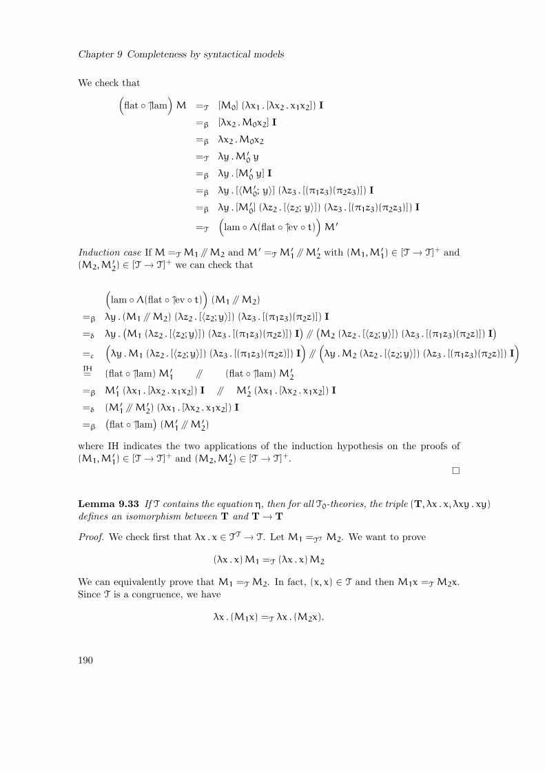
Chapter 9 Completeness by syntactical models
We check that(
flat ↑lam)
M =T [M0] (λx1 . [λx2 . x1x2]) I
=β [λx2 .M0x2] I
=β λx2 .M0x2
=T λy .M ′0 y
=β λy . [M ′0 y] I
=β λy . [〈M ′0; y〉] (λz3 . [(π1z3)(π2z3)]) I
=β λy . [M ′0] (λz2 . [〈z2; y〉]) (λz3 . [(π1z3)(π2z3)]) I
=T
(
lam Λ(flat ↑ev t))
M ′
Induction case If M =T M1 //M2 and M ′ =T M′1 //M
′2 with (M1,M
′1) ∈ [T → T]+ and
(M2,M′2) ∈ [T → T]+ we can check that
(
lam Λ(flat ↑ev t))
(M1 //M2)
=β λy . (M1 //M2) (λz2 . [〈z2;y〉]) (λz3 . [(π1z3)(π2z)]) I
=δ λy .(
M1 (λz2 . [〈z2;y〉]) (λz3 . [(π1z3)(π2z)]) I)
//(
M2 (λz2 . [〈z2;y〉]) (λz3 . [(π1z3)(π2z)]) I)
=ε
(
λy .M1 (λz2 . [〈z2;y〉]) (λz3 . [(π1z3)(π2z)]) I)
//(
λy .M2 (λz2 . [〈z2;y〉]) (λz3 . [(π1z3)(π2z)]) I)
IH= (flat ↑lam) M ′
1 // (flat ↑lam) M ′2
=β M ′1 (λx1 . [λx2 . x1x2]) I // M ′
2 (λx1 . [λx2 . x1x2]) I
=δ (M ′1 //M
′2) (λx1 . [λx2 . x1x2]) I
=β
(
flat ↑lam)
(M ′1 //M
′2)
where IH indicates the two applications of the induction hypothesis on the proofs of(M1,M
′1) ∈ [T → T]+ and (M2,M
′2) ∈ [T → T]+.
Lemma 9.33 If T contains the equation η, then for all T0-theories, the triple (T, λx . x, λxy . xy)defines an isomorphism between T and T→ T
Proof. We check first that λx . x ∈ TT→ T. Let M1 =TT M2. We want to prove
(λx . x)M1 =T (λx . x)M2
We can equivalently prove that M1 =T M2. In fact, (x, x) ∈ T and then M1x =T M2x.Since T is a congruence, we have
λx . (M1x) =T λx . (M2x).
190

9.4 Completeness
Using the η rule we conclude that M1 =T M2.We check that
lam app =β λz . lam(z)
=β λz . λy . zy
=η λz . z
9.4.6 Completeness result
To conclude the proof of Theorem 9.28, we need to ensure that the congruence inducedby the model D is precisely the congruence T. This relies on the following lemma:
Lemma 9.34 Let ℓ = [x1, . . . , xn] be a list of variables. For all terms M such thatFV (M) ⊂ ℓ, we have:
JMKDℓ =βδ λz .Mx1 := π
x1
ℓ z; . . . ; xn := πxn
ℓ z
(where z is a fresh variable).
Proof. We prove the result by induction on M. We only check the result for the lastcase that is, if M = M1 //M2 then we have
JM1 //M2KDℓ = par 〈JM1K
Dℓ ; JM2K
Dℓ 〉
IH=βδ par 〈λz .M1x1 := π
x1
ℓ (z); . . . ; xn := πxn
ℓ (z);
λz .M2x1 := πx1
ℓ (z); . . . ; xn := πxn
ℓ (z)〉
=β λy . par (λp . p (M1x1 := πx1
ℓ (y); . . . ; xn := πxn
ℓ (y))
(M2x1 := πx1
ℓ (y); . . . ; xn := πxn
ℓ (y)))
=β λy .flat u(λp . p (M1x1 := πx1
ℓ (y); . . . ; xn := πxn
ℓ (y))
(M2x1 := πx1
ℓ (y); . . . ; xn := πxn
ℓ (y)))
=β λy .(
[M1x1 := πx1
ℓ (y); . . . ; xn := πxn
ℓ (y)] //
[M2x1 := πx1
ℓ (y); . . . ; xn := πxn
ℓ (y)])
I
=δ λy . [M1x1 := πx1
ℓ (y); . . . ; xn := πxn
ℓ (y)] I //
[M2x1 := πx1
ℓ (y); . . . ; xn := πxn
ℓ (y)] I
=β λy .M1x1 := πx1
ℓ (y); . . . ; xn := πxn
ℓ (y) //
M2x1 := πx1
ℓ (y); . . . ; xn := πxn
ℓ (y)
= λy . (M1 //M2)x1 := πx1
ℓ (y); . . . ; xn := πxn
ℓ (y)
191
Chapter 9 Completeness by syntactical models
Theorem 9.35 (Completeness) For all lists of variables ℓ, and for all terms M1 andM2 such that FV (M1) ∪ FV (M2) ⊂ ℓ, one has
JM1KDℓ = JM2K
Dℓ iff M1 =T M2 .
Proof. The soudness proposition gives one implication. We show the other one. Let usassume that JM1K
Dℓ = JM2K
Dℓ and l = [x1, . . . , xn]. Since D is a congruence we have
〈x1, . . . , xn〉 ∈ Dn (by abuse we denote by l this term). We check that
M1 = M1x1 := x1; . . . ; xn := xn
=β M1x1 := πx1
ℓ (l); . . . ; xn := πxn
ℓ (l)
=β
(
λz .M1x1 := πx1
ℓ (z); . . . ; xn := πxn
ℓ (z))
l
=βδ JM1KDℓ l
=T JM2KDℓ l
=βδ M2
Conclusion
In the previous chapter, we introduce a sound categorical semantics for the parallel λ-calculus that we proved here its completeness. In the following chapters, we give twoabstract methods to build such models.
192

Chapter 10
Constructing a model of the parallelλ-calculus
Context We have defined a sound and complete categorical semantics for the parallelλ-calculus. We have given in Chapter 8 several examples of models of the parallel λ-calculus in the category of Scott domains.
Contributions We present two methods for constructing a model of the parallel λ-calculus from a given ccc and a given strong aggregation monad. Both constructionmethods rely on the existence of objects satisfying particular equations. They can befruitfully used in the category of Scott domains where such equations have many inter-esting solutions.
Outline of the chapter We give a first method in Section 10.1 and a second one inSection 10.2.
10.1 First method
In this section, we assume that C is a Cartesian closed category equipped with a strongaggregation monad (T, η, µ, t, u). Our aim is to show that
Theorem 10.1 If D ∈ ObjC is such that D ∼= (TD)D, then D can be given all thestructures of a model of the parallel λ-calculus.
The rest of this section is devoted to the proof of Theorem 10.1. We can notice thatwe will never use the hypothesis (agg-t) and (agg-µ).
In what follows, we assume that D is an object equipped with a pair of arrows
Dunfold //
(TD)D
foldoo
such that unfold fold = idTDD and fold unfold = idD.
193

Chapter 10 Constructing a model of the parallel λ-calculus
10.1.1 Algebraicity
The arrow flat ∈ C[T(D);D] is defined by
flat = fold Λ(µ Tev t) Tunfold
Its construction is depicted below:
T(D)
Tunfold
D
T(
(TD)D) Λ(µTev t) // (TD)D
fold
OO
T(
(TD)D)
×Dt
// T(
(TD)D ×D)
Tev// T2(D) µ
// T(D)
We check that
flat η = fold Λ(µ Tev t) Tunfold η= fold Λ(µ Tev t) η unfold (nat-η)= fold Λ
(
µ Tev t (η× id))
unfold (exp-)= fold Λ
(
µ Tev η)
unfold (str-η)= fold Λ
(
µ η ev)
unfold (nat-η)= fold Λ
(
ev)
unfold (mon-2)
= fold unfold (exp-η)= id (fold/unfold)
Writing f = Λ(µ Tev t), we check that
flat Tflat = fold f Tunfold T(fold f Tunfold)
= fold Λ(µ Tev t) Tf T2unfold (fold/unfold)
= fold Λ(µ Tev t (Tf× id)) T2unfold (exp-nat)= fold Λ(µ Tev T(f× id) t) T2unfold (t-nat)= fold Λ(µ T(µ Tev t) t) T2unfold (exp-β)
= fold Λ(µ µ T2ev Tt t) T2unfold (mon-3)
= fold Λ(µ Tev µ Tt t) T2unfold (µ-nat)= fold Λ(µ Tev t (µ× id)) T2unfold (str-µ)
= fold Λ(µ Tev t) µ T2unfold (exp-)= fold Λ(µ Tev t) Tunfold µ = flat µ (µ-nat)
10.1.2 Reflexivity
Once the structure of T-algebra of D has been outlined, it is easy to check that D isa reflexive object of the category. For that, we define two arrows lam ∈ C[DD;D] andapp ∈ C[D;DD] by setting:
lam = fold Λ(η ev) and app = Λ(flat ev) unfold .
194

10.1 First method
The construction of these arrows is depicted below:
lam =
DDΛ(η ev) // (TD)D fold // D
DD ×D ev// D η
// T(D)
app =
Dunfold// (TD)D
Λ(flat ev) // DD
(TD)D ×D ev// T(D)
flat// D
We check that
app lam = Λ(flat ev) unfold fold Λ(η ev)
= Λ(flat ev) Λ(η ev) (unfold/fold)
= Λ(
flat ev (Λ(η ev) × id))
(exp-)= Λ(flat η ev) (exp-β)
= Λ(ev) (alg-1)
= id (exp-η)
so that (lam, app) is a retraction of D onto DD.
10.1.3 Distributivity axiom
We prove that the diagram (δ) commutes. We check that
app flat = Λ(flat ev) unfold flat= Λ(flat ev) unfold fold︸ ︷︷ ︸ Λ(µ Tev t) Tunfold (def-flat)
= Λ(flat ev) Λ(µ Tev t) Tunfold (unfold/fold)
= Λ(flat ev Λ(µ Tev t) × id) Tunfold (exp-)= Λ(flat µ Tev t) Tunfold (exp-β)
= Λ(flat Tflat Tev t) Tunfold (alg-2)
= Λ(flat Tev T(Λ(flat ev) × id) t) Tunfold (exp-β)
= Λ(flat Tev t (TΛ(flat ev) × id)) Tunfold (nat-t)= Λ(flat Tev t) TΛ(flat ev) Tunfold (exp-)= Λ(flat Tev t) Tapp (def-app)
10.1.4 Typical use
The typical use of this theorem in the category of Scott domains is the following: as-sume that 〈T, u〉 is a strong aggregation monad in the category of Scott domains whoseunderlying endofunctor T is ωop-continuous (i.e. preserves limits on ωop-chains). Thenthe correspondence
X 7→ (TX)X
induces an ω-cocontinuous (covariant) endofunctor in the category Scottip of Scottdomains equipped with injection-projection pairs. Starting from a domain D0 equipped
195

Chapter 10 Constructing a model of the parallel λ-calculus
with an injection retraction pair D0 (TD0)D0 , it is easy to build a smallest fixpoint
D ≃ (TD)D containing D0 (in the sense of injection-retraction pairs).
Notice that this way of constructing models in the category of Scott domains is notlimited to the lower powerdomain monad Pl, but that it can be also used with:
• The list monad, which defines an associative aggregation monad using the concate-nation function;
• The free magma monad TX, defined as the smallest fixpoint of the equation
TX =(
X+ (TX× TX))
⊥,
that induces an aggregation monad which is neither associative, commutative noridempotent.
10.2 Second method
In this section, we assume that C is a Cartesian closed category equipped with a strongaggregation monad (T, η, µ, t, u) and a T-algebra (R,flatR).
We denote by Dω the infinite product of D. We use the standard functions comingwith infinite products:
hd : Dω→ D = π0
tl : Dω→ Dω = 〈πi+1〉i∈N
cons : D×Dω→ Dω = 〈fi〉i∈N
f0 = π1
fi+1 = πi π2
We will often use the following equation:
cons 〈hd; tl〉 = idDω (prod-i)〈hd; tl〉 cons = idD×Dω
Theorem 10.2 If D ∈ ObjC is such that D ∼= RDωthen D can be given the additional
structures of an ε-model of the parallel λ-calculus.
In what follows we assume that D is an object equipped with a pair of arrows
Dunfold //
RDω
foldoo
such that
unfold fold = idRDω and fold unfold = idD .
196

10.2 Second method
10.2.1 Algebraicity
The arrow flatD ∈ C[T(D);D] is defined by
flatD = fold Λ(flatR Tev t) Tunfold
Its construction is depicted below:
T(D)
Tunfold
D
T(
RDω) Λ(flatR Tev t) // RDω
fold
OO
T(RDω) ×Dω
t// T(RDω
×Dω)Tev
// TRflatR
// R
We check that
flatD η = fold Λ(flatR Tev t) Tunfold η= fold Λ(flatR Tev t) η unfold (nat-η)= fold Λ
(
flatR Tev t (η× id))
unfold (exp-)= fold Λ
(
flatR Tev η)
unfold (str-η)= fold Λ
(
flatR η ev)
unfold (nat-η)= fold Λ
(
ev)
unfold (alg-1)
= fold unfold (exp-η)= id (fold/unfold)
Writing f = Λ(flatR Tev t), we check that
flatD TflatD = fold f Tunfold T(fold f Tunfold)
= fold Λ(flatR Tev t) Tf T2unfold (fold/unfold)
= fold Λ(flatR Tev t (Tf× id)) T2unfold (exp-)= fold Λ(flatR Tev T(f× id) t) T2unfold (t-nat)= fold Λ(flatR T(flatR Tev t) t) T2unfold (exp-β)
= fold Λ(flatR µ T2ev Tt t) T2unfold (alg-2)
= fold Λ(flatR Tev µ Tt t) T2unfold (µ-nat)= fold Λ(flatR Tev t (µ× id)) T2unfold (str-µ)
= fold Λ(flatR Tev t) µ T2unfold (exp-)= fold Λ(flatR Tev t) Tunfold µ = flatD µ (µ-nat)
Note that the proofs of the last two equations are in a one-to-one correspondence withthe one of Theorem 10.1. The morphism µ is replaced here by flatR.
10.2.2 Reflexivity
We check that D is a reflexive object of the category. For that, we define two arrowslam ∈ C[DD;D] and app ∈ C[D;DD] by setting:
lam = fold Λ(ev (ev × id) α (id × 〈hd; tl〉)) Λ(unfold ev)
and app = Λ(fold ev) ΛΛ(ev (id × cons) α) unfold
197

Chapter 10 Constructing a model of the parallel λ-calculus
The construction of these arrows is depicted below:
DDΛ(unfoldev) //
(RDω)D
Λ(foldev)oo
Λ(ev(ev×id)α(id×〈hd;tl〉))
RDω
fold //
ΛΛ(ev(id×cons)α)
OO
Dunfold
oo
We first prove that DD ∼= (RDω)D. We check that
Λ(unfold evD,D) Λ(fold evRDω,D)
= Λ(unfold evD,D Λ(fold evRDω,D) × idD) (exp-)
= Λ(unfold fold evRDω,D) (exp-β)
= Λ(evRDω,D) (fold/unfold)
= id(RDω)D (exp-η)
andΛ(fold evRDω
,D) Λ(unfold evD,D)
= Λ(fold evRDω,D Λ(unfold evD,D) × idD) (exp-)
= Λ(fold unfold evD,D) (exp-β)
= Λ(evD,D) (fold/unfold)= idDD (exp-η)
We now prove that (RDω)D ∼= RDω
. Writing f = ev (ev × id) α (id× 〈hd; tl〉) andg = ev (id × cons) α we check that
Λf ΛΛg(i)= Λ(ev (ev × id) α (id × 〈hd; tl〉) ΛΛg× id) (exp-)= Λ(ev (ev × id) α (ΛΛg× id) (id × 〈hd; tl〉))= Λ(ev (ev × id) ((ΛΛg× id) × id) α (id × 〈hd; tl〉)) (nat-α)(v)= Λ(ev (Λg× id) α (id × 〈hd; tl〉)) (exp-β)(vi)= Λ(ev (id × cons) α︸ ︷︷ ︸
g
α (id × 〈hd; tl〉)) (exp-β)
(vii)= Λ(ev) (prod-i)
= id (exp-η)
The steps from (i) to (vi) are described in Figure 10.1. In this figure, diagram (1) isgiven by trivial properties of products. Diagram (2) is given by the naturality of α.Diagram (3) is given by (exp-β) and (exp-).
The step (vii) is described in Figure 10.2, which expresses easy properties of products.More precisely, this diagram is given by (prod-i).
198

10.2 Second method
RDω×Dω
id×〈hd;tl〉
ΛΛg×id
vvnnnnnnnnnnnnnnnnnnnnnnnnn
(RDω)D ×Dω
id×〈hd;tl〉
RDω× (D×Dω)
α
ΛΛg×id
vvnnnnnnnnnnnnnnnnnnnnnnnn
(RDω)D × (D×Dω)
α
(1)
(RDω×D) ×Dω
(ΛΛg×id)×id
vvnnnnnnnnnnnnnnnnnnnnnnnn
g
((RDω
)D ×D) ×Dω
ev×id
(2)
R
RDω×Dω
ev
66nnnnnnnnnnnnnnnnnnnnnnnnnnnn
(3)
Figure 10.1: Auxiliary diagram for the reflexivity
We finally check that
ΛΛg Λf= ΛΛ(g ((Λf× id) × id)) (exp-)= ΛΛ(ev (id × cons) α ((Λf× id) × id))
= ΛΛ(ev (id × cons) (Λf× id) α) (nat-α)
= ΛΛ(ev (Λf× id) (id × cons) α)
= ΛΛ(ev (ev × id) α (id × 〈hd; tl〉)︸ ︷︷ ︸f
(id × cons) α) (exp-β)
= ΛΛ(ev (ev × id) α α) (prod-i)= ΛΛ(ev (ev × id)) = Λ(ev) = id
10.2.3 Distributivity axiom
Since we have an isomorphism between DD and D then the two diagrams (δ) and (ε)are equivalent. So we only check the first one.
We isolate two parts of the proofs in Figure 10.3 and in Figure 10.4. The proof ofcommutation of the first one is immediate. In Figure 10.4 the first diagram is given
199

Chapter 10 Constructing a model of the parallel λ-calculus
RDω×Dω
id×〈hd;tl〉 // RDω× (D×Dω)
α // (RDω×D) ×Dω
α
vvmmmmmmmmmmmmmmmmmmmmmmmm
RDω×Dω RDω
× (D×Dω)id×cons
oo
Figure 10.2: Auxiliary diagram for reflexivity
by (str-α). Diagram (2) is given by the naturality of t. Diagram (3) is given by thedefinition of g.
We often use the equation
Tev t TΛf× id = Tf t (10.1)
that can be proved using first (nat-t) and then using (exp-β). Writing h = flatRTevt,we check that:
app flatD
= Λ(fold ev) ΛΛg unfold fold Λh Tunfold= Λ(fold ev (ΛΛg× id) Λh× id) Tunfold (exp-)= Λ(fold Λg Λh× id) Tunfold (exp-β)
= Λ(fold Λ(g ((Λh× id) × id))) Tunfold (exp-)= Λ(fold Λ(h (id × cons) α)) Tunfold (Fig. 10.3)= Λ(fold Λ(flatR Tg t (t× id))) Tunfold (Fig. 10.4)= Λ(fold Λ(flatR Tev t TΛg× id (t× id))) Tunfold (Eq. 10.1)= Λ(fold Λ(h TΛg× id (t× id))) Tunfold= Λ(fold Λ(h) Tunfold Tfold Tev t TΛΛg× id) Tunfold (Eq. 10.1)= Λ(fold Λ(h) Tunfold Tev t (TΛ(fold ev) × id) TΛΛg× id) Tunfold (Eq. 10.1)= Λ(flatD Tev t) TΛ(fold ev) TΛΛg Tunfold = Λ(flatD Tev t) Tapp (exp-)
10.2.4 Typical use
In Scott domains, the equation D = R(Dω) always has solutions, since the endofunctorX 7→ R(Xω) is ω-cocontinuous in the category of injection-projection pairs. Notice thatthe least fixpoint D of this functor is not trivial as soon as the algebra R is not trivial.Intuitively, the smallest solution D can be understood as the smallest η-model of theparallel λ-calculus which contains R (in the sense of injection-projection pairs).
Conclusion and Future Works
We have defined a sound and complete categorical semantics for the parallel λ-calculus,based on a notion of aggregation monad which is modular w.r.t. associativity, commu-
200

10.2 Second method
((RDω) ×D) ×Dω
α
(T(RDω) ×D) ×Dω
α
(Λh×id)×idoo
(RDω) × (D×Dω)
id×cons
T(RDω) × (D×Dω)
id×cons
Λh×idoo
RDω×Dω
ev
T(RDω) ×DωΛh×idoo
h
rreeeeeeeeeeeeeeeeeeeeeeeeeeeeeeeee
R
Figure 10.3: Auxiliary diagram for the distributivity
(T(RDω) ×D) ×Dω α //
t×id
T(RDω) × (D×Dω)
t
wwpppppppppppppppppppppp
id×cons
%%LLLLLLLLLLLLLLLLLLLL
(2)T(RDω×D) ×Dω
t
(1)
T(RDω× (D×Dω))
T(id×cons)
''NNNNNNNNNNNNNNNNNNNNNN
(3)
T(RDω) ×Dω
t
yyrrrrrrrrrrrrrrrrrrrr
T((RDω×D) ×Dω)
Tα
77pppppppppppppppppppppp
Tg
''OOOOOOOOOOOOOOOOOOOOOOOT(RDω
×Dω)
Tev
wwooooooooooooooooooooooo
TR
Figure 10.4: Auxiliary diagram for the distributivity
201

Chapter 10 Constructing a model of the parallel λ-calculus
tativity and idempotence.To prove completeness, we have introduced a category of partial equivalence relations
adapted to parallelism, in which any extension of the basic equational theory of thecalculus is induced by some model.
We have also presented abstract methods to construct models of the parallel λ-calculusin categories where particular equations have solutions, such as the category of Scottdomains and its variants, and check that G. Boudol’s original semantics is a particularcase of ours.
This work on the denotational semantics of the parallel λ-calculus is initially motivatedby the semantical study of the ρ-calculus [CK01], a formalism which combines ML-stylepattern-matching with parallel aggregation. The next step is thus to find a satisfyingway to integrate constructors and pattern-matching in our setting. However, combiningpattern-matching with parallel aggregation naturally raises new problems related toadditivity. To understand this point, let us consider the following example.
Assume that the parallel λ-calculus is enriched with two constant constructors a, band a unary constructor c( ), plus a syntactic construct [c(x) ≪ N]M that matches theterm N against the pattern c(x), and binds all free occurrences of x inM to the argumentof the destructed value. (We do not give any special meaning to this construction whenNis not a constructed value.)
Now consider the term M = [c(x) ≪ c(a // b)] F x x, where F is an arbitrary function.The naive way to reduce M is to substitute the term (a // b) to x in the r.h.s. F x x,hence:
[c(x) ≪ c(a // b)] F x x → F (a // b) (a // b) .
(This strategy is the one which is actually implemented by the standard encodings ofconstructed values and pattern-matching in the λ-calculus.)
However, it is also legitimate to consider that a and b represent two possible choicesfor the argument of the constructed value c(a//b). Following this intuition, a completelydifferent reduction strategy is to distribute a and b w.r.t. the matching construct, whichyields:
[c(x) ≪ c(a // b)]F x x → F aa // F bb .
Of course, both design choices are clearly incompatible, which is easy to see by takingF = λxy . xy. This second strategy—which seems to be impossible to simulate in thecore parallel λ-calculus—is much more interesting, since it suggests that both operationsof construction and destruction are linear:
c(N1 // N2) = c(N1) // c(N2)
[c(x) ≪ (N1 // N2)]M = [c(x) ≪ N1]M// [c(x) ≪ N2]M
This example naturally raises the exciting challenge of constructing a model of the ρ-calculus that implements the second reduction strategy, while being rich enough to reflectall the expressivity of ML-style pattern-matching, such as the existence of infinitelymany constructors of all arities (with pairwise disjoint images), the existence of variadicconstructors, etc.
202
Quatrieme partie
Epilogue
203


Conclusion et travaux futurs
Dans la premiere partie de cette these, nous avons introduit une nouvelle approchepour resoudre des equations de filtrage dans le λ-calcul. La methode utilisee n’est pas de-pendante d’un systeme de types particulier et possede de plus l’avantage, contrairementaux autres approches [Hue76, HL78, CQS96], de ne pas introduire de nouvelles variablesde filtrage durant le processus de resolution. Bien que l’ensemble des equations resoluessoit particulierement riche (equations du second-ordre et equations sur des motifs a laMiller entre autres), l’utilisation du λ-calcul comme langage support est restrictif.
Tout d’abord, dans le cadre de la transformation de programmes et dans le cadre de lapreuve (calcul des constructions avec filtrage par exemple), il est fondamental de disposerd’algorithmes pour le filtrage modulo βη en presence de symboles AC. Une telle extensionde l’algorithme du second-ordre de G. Huet et de B. Lang a ete proposee [Cur93] mais ilserait particulierement interessant d’etudier le filtrage modulo super-developpements enpresence de symboles AC et de le comparer avec l’approche precedente. Un tel algorithmeutilisant les super-developpements semble a priori plus simple a mettre en pratique.
D’autre part, lorsque l’on souhaite transformer des programmes fonctionnels nonstricts1 (programmes comme ρ-termes), ou lorsque l’on considere [Wac05] des termesde preuve riches pour la deduction modulo (preuves comme ρ-termes), la β-equationdu λ-calcul doit etre remplacee par la theorie equationnelle du ρ-calcul. Ainsi defini, unalgorithme pour le filtrage d’ordre superieur modulo super-developpements permettraitde faire l’economiede l’encodage, souvent couteux [MS01], du filtrage.
Les outils pour le filtrage d’ordre superieur que nous avons introduits dans cette theseont des applications nombreuses et plus particulierement dans le cadre de la preuve deproprietes de programme. En se basant sur un ensemble de regles de transformationspreservant la semantique des programmes et en utilisant, pour appliquer ces regles, unalgorithme de filtrage certifie, on peut ainsi prouver des proprietes sur des programmessemantiquement equivalents mais plus simples. Considerons par exemple les deux al-gorithmes classiques pour renverser les listes : l’algorithme naıf mais defini simplementpar filtrage sur la structure de donnees liste et l’algorithme efficace utilisant une pileauxiliaire. L’approche que nous avons decrite consiste a prouver d’abord les proprietessouhaitees sur l’algorithme naıf (ce qui est toujours plus simple) puis, par transformationde programmes prouvee correcte et complete, on peut « heriter » de ces proprietes surla version efficace.
Dans la deuxieme partie de cette these, nous avons etudie le filtrage et les substitu-tions, mecanismes de base des calculs d’ordre superieur avec motifs comme le ρ-calcul, le
1c’est-a-dire utilisant primitivement un mecanisme de filtrage
205
Conclusion et travaux futurs
calcul pur de motifs [JK06] et le λ-calcul avec motifs [Oos90]. Nous avons tout d’abordintroduit un calcul avec filtrage et substitutions explicites, donnant un cadre permettantde souligner les interactions possibles et, offrant un support pour l’implementation detels calculs.
Ce calcul ne traite pas explicitement l’α-conversion. Nous avons esquisse une versiongeneralisee des substitutions explicites avec indices de de Bruijn adaptee aux calculsayant des constructions pouvant lier plusieurs variables simultanement. D’autres ap-proches peuvent etre adaptees pour ces langages : le λ-calcul avec operateur explicitede portee [HO03], les directeurs qui sont utilises pour la reecriture d’ordre superieurdans [Sin05] ou encore les reseaux d’interactions qui ont ete etudies dans le cadre duρ-calcul dans [FMS05, CFF+06].
Nous avons mis en avant l’importance de l’etude modulaire des calculs avec motifset nous avons isole les proprietes cles des algorithmes de filtrage permettant d’obtenirdes calculs coherents (confluents). Ces calculs avec motifs peuvent manipuler des mo-tifs dynamiques, c’est-a-dire qui peuvent etre instancies et reduits. Ils conduisent a deslangages fonctionnels avec de nouvelles formes de polymorphisme [Jay04].
Notre etude s’est limitee au cas du filtrage unitaire (au plus une solution). Pourtant enpratique, l’utilisation du filtrage modulo une theorie equationnelle permet d’ecrire desprogrammes hautement declaratifs, comme c’est la cas dans le langage Tom [BBK+06]implementant le filtrage sur les listes (filtrage associatif avec element neutre). Neanmoins,l’extension de l’etude realisee ici au cas du filtrage non-unitaire necessite une compre-hension nouvelle du mecanisme de filtrage et plus particulierement dans son interactionavec les collections de resultats (indispensables dans le cas du filtrage non-unitaire).
Dans la troisieme partie de cette these, nous avons mis en evidence que l’ajout decollections de termes distributifs par rapport a l’application est non triviale meme dansle cadre du λ-calcul. Nous avons montre que les collections de termes, la structure duρ-calcul ou encore l’operateur de parallelisme du λ-calcul parallele [Bou94] conduisent ala notion plus generale d’agregation.
Nous avons donc introduit une semantique categorique correcte et complete du λ-calcul avec operateur de parallelisme. Cette semantique repose fortement sur la notiond’agregation et de termes lineaires. Les exemples de modeles que nous avons donnes sontessentiellement des domaines de Scott mais les modeles de la logique lineaire qui validentla regle Mix et les modeles du λ-calcul differentiel [ER03, Ehr05, Ehr02] sont clairementde bons candidats.
L’etape suivante est donc d’integrer les constructeurs et le filtrage de maniere satisfai-sante dans notre cadre. Nous retrouvons naturellement les problemes lies a la combinaisondu filtrage avec les collections de resultats et que nous avons mentionnes dans la deuxiemepartie de cette these. Cette combinaison se traduit dans notre cadre semantique par denouveaux problemes lies a la linearite des constructeurs et du filtrage.
Dans cette these, nous avons, en resume, cherche a expliciter les mecanismes fon-damentaux des calculs avec motifs en utilisant une approche operationnelle et denota-tionnelle. L’etude du calcul de reecriture qui est a l’origine des travaux presentes ici
206
avait ete realisee pour donner une semantique aux langages bases sur la reecriture, lesstrategies [BKK96, Vis01b, KK04, Kir05, MOMV06] jouant un role particulierementimportant dans tous ces langages (Tom, Elan, Maude, Stratego etc).
Integrees en effet aux langages generalistes comme Java, les notions de base de lareecriture comme le filtrage et les strategies, permettent d’introduire dans ces langagesdes ılots formels [BKM06]. Ceci est particulierement important pour pouvoir developperdes parties de code fortement sensibles, c’est-a-dire dont la securite (certification etsurete) est cruciale. C’est par exemple le cas pour l’implementation des politiques desecurite [DKKS07]. La reecriture et les strategies ainsi que la notion d’ılots formelsdonnent des outils particulierement novateurs et efficaces.
Dans ce contexte particulierement riche, il nous apparaıt maintenant indispensable derevenir aux motivations initiales du ρ-calcul pour approfondir la semantique des strate-gies. Plusieurs pistes sont possibles. L’etude de la semantique denotationnelle des calculsavec motifs, initialisee dans cette these, en est une. Une autre approche est l’utilisationde la reecriture de dimension superieure [Bur93, Laf97, Gui04, Gui06b, Gui06a] offrantun langage a la fois algebrique, graphique et topologique commun aux structures, auxcalculs et aux demonstrations. Les regles de reecriture etant, dans ce formalisme, desobjets de dimension 3, on peut envisager de considerer [Gui04] les strategies comme desobjets de dimension 4. Bien que tres prospective, cette approche paraıt particulierementprometteuse.
207

Conclusion et travaux futurs
208

Bibliographie
[Abr91] Samson Abramsky – « Domain theory in logical form », Annals of Pureand Applied Logic 51 (1991), no. 1–2, p. 1–77. 173
[AC96] Martın Abadi et Luca Cardelli – A theory of objects, Springer-Verlag,New York, 1996. 78
[AC98] Roberto Amadio et Pierre-Louis Curien – Domains and lambda-calculi,Cambridge Tracts in Theoretical Computer Science, vol. 46, CambridgeUniversity Press, Cambridge, 1998. 147, 148, 151, 171
[ACCL91] Martın Abadi, Luca Cardelli, Pierre-Louis Curien et Jean-JacquesLevy – « Explicit substitutions », Journal of Functional Programming 1(1991), no. 4, p. 375–416. 7, 87, 120
[Acz78] Peter Aczel – « A general Church-Rosser theorem », Tech. report, Univer-sity of Manchester, July 1978. 7, 29
[ADGR07] Jeremy Avigad, Kevin Donnelly, David Gray et Paul Raff – « A for-mally verified proof of the prime number theorem. », ACM Transactions onComputational Logic, To appear. (2007). 11
[AL91] Andrea Asperti et Guiseppe Longo – Categories, types and structures,MIT Press, 1991. 147
[All78] John Allen – Anatomy of LISP, McGraw-Hill, Inc., New York, USA, 1978.5
[AMR06] Ariel Arbiser, Alexandre Miquel et Alejandro Rıos – « A lambda-calculuswith constructors », Term Rewriting and Applications – RTA’06 (Seattle,USA), Lecture Notes in Computer Science, vol. 4098, Springer, August 2006,p. 181–196. 8, 12, 125, 142, 143
[AO93] Samson Abramsky et Luke Ong – « Full abstraction in the lazy lambdacalculus », Information and Computation 105 (1993), no. 2, p. 159–267. 173
[Bal06] Vincent Balat – « Ocsigen : Typing web interaction with objective caml »,ACM Sigplan Workshop on ML, 2006. 12
[Bar84] Henk Barendregt – The Lambda-Calculus, its syntax and semantics, Stu-dies in Logic and the Foundation of Mathematics, North Holland, 1984,Second edition. 17, 20, 22, 23, 69, 147
[Bar91] Franco Barbanera – « Adding algebraic rewriting to the calculus ofconstructions : Strong normalization preserved », Conditional and TypedRewriting Systems -CTRS’90 (S. Kaplan et M. Okada, eds.), LectureNotes in Computer Science, vol. 516, Springer, 1991, p. 262–271. 11, 12
209

Bibliographie
[Bar92] Henk Barendregt – « Handbook of logic in computer science »,ch. Lambda Calculi with Types, p. 117–309, Clarendon Press, 1992. 17
[Bax77] Lewis Denver Baxter – « The complexity of unification. », These de doc-torat, University of Waterloo, 1977. 62
[BBCK04] Clara Bertolissi, Paolo Baldan, Horatiu Cirstea et Claude Kirchner
– « A rewriting calculus for cyclic higher-order term graphs », Proceedings ofthe 2nd International Workshop on Term Graph Rewriting (Roma (Italy))(M. Fernandez, ed.), Electronic Notes in Theoretical Computer Science,September 2004, to appear. 67
[BBCK06] Paolo Baldan, Clara Bertolissi, Horatiu Cirstea et Claude Kirchner
– « A rewriting calculus for cyclic higher-order term graphs », MathematicalStructures in Computer Science (2006). 5
[BBK+06] Emilie Balland, Paul Brauner, Radu Kopetz, Pierre-Etienne Moreau
et Antoine Reilles – « The Tom manual », 2006, http://tom.loria.fr/soft/release-2.4/manual-2.4/index.html. 7, 88, 118, 144, 206
[BCK06] Clara Bertolissi, Horatiu Cirstea et Claude Kirchner – « Expres-sing combinatory reduction systems derivations in the rewriting calculus »,Higher-Order and Symbolic Computation 19 (2006), no. 4, p. 345–376. 31,64, 67
[BCKL03] Gilles Barthe, Horatiu Cirstea, Claude Kirchner et Luigi Liquori –« Pure patterns type systems », Principles of Programming Languages -POPL’03, vol. 38, ACM, January 2003. 5, 8, 67, 125, 137, 140
[BCL99] Gerard Boudol, Pierre-Louis Curien et Carolina Lavatelli – « A se-mantics for lambda calculi with resources », Mathematical Structures inComputer Science 9 (1999), no. 4, p. 437–482. 9, 155
[BDL06] Sandrine Blazy, Zaynah Dargaye et Xavier Leroy – « Formal verificationof a C compiler front-end », Formal Methods, 14th International Symposiumon Formal Methods, Lecture Notes in Computer Science, vol. 4085, 2006,p. 460–475. 11
[Ber05] Clara Bertolissi – « The graph rewriting calculus : properties and expres-sive capabilities », These de doctorat, Institut National Polytechnique deLorraine - INPL, Oct 2005. 5, 67
[BF82] Klaus Berkling et Elfriede Fehr – « A consistent extension of the lambda-calculus as a base for functional programming languages », Information andControl 55 (1982), no. 1-3, p. 89–101. 122
[BHK07] Paul Brauner, Clement Houtmann et Claude Kirchner – « Principles ofsuperdeduction », Logics in Computer Science - LICS’07, 2007, To appear.117
[BJKO00] Mark van den Brand, Hayco Jong, Paul Klint et Pieter Olivier – « Ef-ficient Annotated Terms », Software, Practice & Experience 30 (2000),p. 259–291. 118
210

Bibliographie
[BK07] Clara Bertolissi et Claude Kirchner – « The rewriting calculus as a com-binatory reduction system », Foundations of Software Science and Compu-tation Structures - FoSSaCS’07 (Braga, Portugal), Lecture Notes in Com-puter Science, Springer, March 2007. 8, 67, 125
[BKK96] Peter Borovansky, Claude Kirchner et Helene Kirchner – « Control-ling Rewriting by Rewriting », 1st International Workshop on RewritingLogic – WRLA’96 (Asilomar (CA, USA)) (J. Meseguer, ed.), vol. 4, Elec-tronic Notes in Theoretical Computer Science, September 1996. 11, 67, 99,207
[BKK98a] Peter Borovansky, Claude Kirchner et Helene Kirchner – « A func-tional view of rewriting and strategies for a semantics of ELAN », TheThird Fuji International Symposium on Functional and Logic Programming(Kyoto) (M. Sato et Y. Toyama, eds.), World Scientific, April 1998, Alsoreport LORIA 98-R-165, p. 143–167. 67, 122
[BKK+98b] Peter Borovansky, Claude Kirchner, Helene Kirchner, Pierre-EtienneMoreau et Christophe Ringeissen – « An overview of ELAN », Workshopon Rewriting Logic and its Applications - WRLA’98, vol. 15, ElectronicNotes in Theoretical Computer Science, September 1998. 118
[BKM06] Emilie Balland, Claude Kirchner et Pierre-Etienne Moreau – « Formalislands », Proceedings of Algebraic Methodology and Software Technology -AMAST’06 (M. Johnson et V. Vene, eds.), LNCS, sv, july 2006. 207
[Bla05] Frederic Blanqui – « Definitions by rewriting in the calculus of construc-tions », Mathematical Structures in Computer Science 15 (2005), no. 1,p. 37–92. 11
[BMV05] Mark van den Brand, Pierre-Etienne Moreau et Jurgen Vinju – « Agenerator of efficient strongly typed abstract syntax trees in java », IEEProceedings - Software Engineering 152 (2005), no. 2, p. 70–78. 118
[Bou94] Gerard Boudol – « Lambda-calculi for (strict) parallel functions », Infor-mation and Computation 108 (1994), no. 1, p. 51–127. 9, 155, 173, 206
[Bru72] Nicolas G. de Bruijn – « A lambda calculus notation with nameless dum-mies, a tool for automatic formula manipulation, with application to thechurch-rosser theorem », Indagationes Mathematicae 34 (1972), p. 381–392.122
[Bru78] — , « Lambda calculus with namefree formulas involving symbols that re-present reference transforming mappings », Indagationes Mathematicae 40(1978), p. 348–356. 119
[Bur90] Hans-Jurgen J. Burckert – « Matching — A special case of unification ? »,Unification, Academic Press, 1990, p. 125–138. 46
[Bur93] Albert Burroni – « Higher-dimensional word problems with applications toequational logic », Theoretical Computer Science 115 (1993), no. 1, p. 43–62. 207
211

Bibliographie
[CDE+02] Manuel Clavel, Francisco Duran, Steven Eker, Patrick Lincoln, Nar-ciso Martı-Oliet, Jose Meseguer et Jose F. Quesada – « Maude : speci-fication and programming in rewriting logic », Theoretical Computer Science285 (2002), no. 2, p. 187–243. 144
[CF07] Horatiu Cirstea et Germain Faure – « Confluence of pattern-basedlambda-calculi », Rewriting Techniques and Applications - RTA’07, vol.4533, 2007, p. 78–92. 8
[CFF+06] Horatiu Cirstea, Germain Faure, Maribel Fernandez, Ian Mackie etFrancois-Regis Sinot – « From functional programs to interaction nets viathe rewriting calculus », Workshop on Reduction Strategies in Rewriting andProgramming - WRS’06, Electronic Notes in Theoretical Computer Science,2006. 206
[CFK04] Horatiu Cirstea, Germain Faure et Claude Kirchner – « A rho-calculusof explicit constraint application », Proceedings of the Workshop on Re-writing Logic and Applications - WRLA’04 (Barcelona (Spain)), ElectronicNotes in Theoretical Computer Science, Mars 2004. 88, 95, 99
[CFK07] — , « A rho-calculus of explicit constraint application », Higher-Order andSymbolic Computation 20 (2007). 88
[CHL96] Pierre-Louis Curien, Therese Hardin et Jean-Jacques Levy –« Confluence properties of weak and strong calculi of explicit substitutions »,Journal of the ACM (JACM) 43 (1996), no. 2, p. 362–397. 100, 101, 117,120, 134
[Chu36] Alonzo Church – « A note on the entscheidungsproblem. », Journal Sym-bolic Logics 1 (1936), no. 1, p. 40–41. 5
[Chu41] — , The Calculi of Lambda Conversion, Princeton University Press, Prin-ceton, 1941. 5
[CHW06] Horatiu Cirstea, Clement Houtmann et Benjamin Wack – « Distributiverewriting calculus », Sixth International Workshop on Reduction Strategiesin Rewriting and Programming – WRLA’06, Electronic Notes in TheoreticalComputer Science, 2006. 5, 76, 82
[Cir00] Horatiu Cirstea – « Calcul de reecriture : fondements et applications »,These de Doctorat, Universite Henri Poincare - Nancy I, 2000. 5, 12, 67,76, 120, 122
[CK98a] Horatiu Cirstea et Claude Kirchner – « The Rewriting Calculus as aSemantics of ELAN », 4th Asian Computing Science Conference (Manila,The Philippines) (J. Hsiang et A. Ohori, eds.), Lecture Notes in ComputerScience, vol. 1538, Springer-Verlag, December 1998. 12, 67
[CK98b] — , « ρ-calculus. Its Syntax and Basic Properties », Workshop Constructionof Computational Logics - CCL’98 (Jerusalem, Israel), September 1998. 5
[CK01] — , « The rewriting calculus — Part I and II », Logic Journal of the InterestGroup in Pure and Applied Logics 9 (2001), p. 427–498. 5, 8, 12, 67, 76, 78,82, 125, 126, 202
212

Bibliographie
[CKL01] Horatiu Cirstea, Claude Kirchner et Luigi Liquori – « Matching Po-wer », Rewriting Techniques and Applications - RTA’01 (Utrecht (The Ne-therlands)), Lecture Notes in Computer Science, Springer-Verlag, May 2001.5, 67, 78
[CKL02] — , « Rewriting Calculus with(out) Types », Workshop on Rewriting Logicand its Applications - WRLA’2002, Pisa, Italy, ENTCS, September 2002.7, 67, 87
[CKLW03] Horatiu Cirstea, Claude Kirchner, Luigi Liquori et Benjamin Wack –« Rewrite strategies in the rewriting calculus », Third International Work-shop on Reduction Strategies in Rewriting and Programming (Valencia,Spain) (B. Gramlich et S. Lucas, eds.), Electronic Notes in TheoreticalComputer Science, June 2003. 74, 79
[CLW03] Horatiu Cirstea, Luigi Liquori et Benjamin Wack – « Rewriting calculuswith fixpoints : Untyped and first-order systems », Types for Proofs andPrograms - TYPES’03 (Torino, Italy), Lecture Notes in Computer Science,vol. 3085, Springer, May 2003, p. 147–161. 8, 79, 80, 82, 125, 128, 135
[CMV+06] Francois Clement, Vincent Martin, Arnaud Vodicka, Roberto DiCosmo et Pierre Weis – « Domain decomposition and skeleton program-ming with ocamlp3l. », Parallel Computing 32 (2006), no. 7-8, p. 539–550.12
[Coq07] The Coq Development Team LogiCal Project – « Coq proof assis-tant reference manual », 2007. 118
[CP88] Thierry Coquand et Christine Paulin – « Inductively defined types. »,Conference on Computer Logic – CCL’88, Lecture Notes in ComputerScience, vol. 417, Springer, 1988, p. 50–66. 12
[CQS96] Regis Curien, Zhenyu Qian et Hui Shi – « Efficient second-order mat-ching », Rewriting Techniques and Applications - RTA’96, Lecture Notes inComputer Science, vol. 1103, 1996. 59, 205
[CR36] Alonzo Church et John Barkley Rosser – « Some properties of conver-sion », Trans. Amer. Math. Soc. 40 (1936). 17
[Cur93] Regis Curien – « Second order E-matching as a tool for automated theoremproving », Progress in Artificial Intelligence - EPIA’93) (Porto, Portugal),Lecture Notes in Artificial Intelligence, vol. 727, Springer, 1993. 205
[Des98] Joelle Despeyroux – « Natural semantics : specifications and proofs »,Tech. report, INRIA, Fevrier 1998. 23
[DG01] Rene David et Bruno Guillaume – « A λ-calculus with explicit weakeningand explicit substitution », Mathematical Structures for Computer Science11 (2001), p. 169–206. 87, 117
[DHK00] Gilles Dowek, Therese Hardin et Claude Kirchner – « Higher orderunification via explicit substitutions », Information and Computation 157(2000), no. 1/2, p. 183–235. 46, 87, 117
213
Bibliographie
[DKKS07] Daniel J. Dougherty, Claude Kirchner, Helene Kirchner et AndersonSantana de Oliveira – « Modular access control via strategic rewriting »,Proceedings of 12th European Symposium On Research In Computer Secu-rity (ESORICS’07) (Dresden), Sep 2007, to appear. 207
[Dow94] Gilles Dowek – « Third order matching is decidable », Annals of Pure andApplied Logic 69 (1994), p. 135–155. 35
[Dow01] — , « Higher-order unification and matching », Handbook of AutomatedReasoning, Elsevier, 2001. 40
[Ehr02] Thomas Ehrhard – « On kothe sequence spaces and linear logic. », Ma-thematical Structures in Computer Science 12 (2002), no. 5, p. 579–623.206
[Ehr05] — , « Finiteness spaces. », Mathematical Structures in Computer Science15 (2005), no. 4, p. 615–646. 206
[Eke95] Steven Eker – « Associative-commutative matching via bipartite graphmatching », Computer Journal 38 (1995), no. 5, p. 381–399. 7, 87
[ER03] Thomas Ehrhard et Laurent Regnier – « The differential lambda-calculus. », Theoretical Computer Science 309 (2003), no. 1-3, p. 1–41. 206
[Fau06] Germain Faure – « Matching modulo superdevelopments application tosecond-order matching », 13th International Conference on Logic for Pro-gramming, Artificial Intelligence, and Reasoning - LPAR’06, Lecture Notesin Computer Science, vol. 4246, Springer, 2006, p. 60–74. 32
[Fau07] — , « Matching modulo superdevelopments application to second-order mat-ching », Journal of Automated Reasonning Submited (2007). 32
[Fer93] Maribel Fernandez – « Modeles de calculs multiparadigmes fondes sur lareecriture », These de doctorat, Universite Paris-Sud, Orsay, France, De-cember 1993. 11
[Fil03] Jean-Christophe Filliatre – « Why : a multi-language multi-prover veri-fication tool », Tech. Report 1366, Universite Paris Sud, 2003. 11
[FK02] Germain Faure et Claude Kirchner – « Exceptions in the rewriting cal-culus », Proceedings of the Rewriting Techniques and Applications - RTA’02(Copenhagen) (S. Tison, ed.), LNCS, Springer-Verlag, July 2002, p. pp. 67,122
[Fly07] Project Flyspeck – « http://www.math.pitt.edu/~thales/flyspeck/ »,Tech. report, 2007. 11
[FM07] Germain Faure et Alexandre Miquel – « A categorical semantics of theparallel lambda-calculus », 2007, Submited. 9, 147
[FMS05] Maribel Fernandez, Ian Mackie et Francois-Regis Sinot – « Interactionnets vs. the rho-calculus : Introducing bigraphical nets », 12th InternationalWorkshop on Expressiveness in Concurrency - EXPRESS’05, ElectronicNotes in Theoretical Computer Science, Elsevier, 2005. 206
214

Bibliographie
[Fri06] Alain Frisch – « Ocaml + xduce. », 11th ACM SIGPLAN InternationalConference on Functional Programming - ICFP’06, 2006, p. 192–200. 12
[Gan80] Robin Gandy – « Proof of strong normalisation », Essays on CombinatoryLogic, Lambda Calculus, and Formalism (J. P. Seldin et J. R. Hindley,eds.), Academic Press inc., New York (NY, USA), 1980. 20
[Gol81] Donald Goldfarb – « The undecidability of the second order unification »,Journal of Theoretical Computer Science 13 (1981), p. 225–230. 35
[Gon05] Georges Gonthier – « A computer-checked proof of the four colour theo-rem », Tech. report, Microsoft Research Cambridge, 2005. 11
[Gui04] Yves Guiraud – « Presentations d’operades et systemes de reecriture »,These, Universite Montpellier 2, June 2004. 207
[Gui06a] — , « Termination orders for 3-polygraphs », Comptes-Rendus de l’Academiedes Sciences - Serie I 342 (2006), no. 4, p. 219–222. 207
[Gui06b] — , « Termination orders for three-dimensional rewriting », Journal of Pureand Applied Algebra 207 (2006), no. 2, p. 341–371. 207
[GWZ02] Herman Geuvers, Freek Wiedijk et Jan Zwanenburg – « A constructiveproof of the fundamental theorem of algebra without using the rationals. »,Types for Proofs and Programs - TYPES’00, Lectures Notes in ComputerScience, vol. 2277, 2002. 11
[Hag90] Masami Hagiya – « Programming by example and proving by exampleusing higher-order unification », 10th International Conference on Automa-ted Deduction - CADE’90 (M. E. Stickel, ed.), Springer-Verlag, July 1990,p. 588–602. 31
[Hin78] J. Roger Hindley – « Standard and normal reductions », Transactions ofthe American Mathematical Society 241 (1978), p. 253–271. 17
[HJM06] Therese Hardin, Mathieu Jaume et Charles Morisset – « Access controland rewrite systems », Proceedings of the 1st International Workshop onSecurity and Rewriting Techniques (SecReT’06) (Venice, Italy), July 2006.11
[HL78] Gerard Huet et Bernard Lang – « Proving and applying program trans-formations expressed with second-order patterns », Acta Informatica 11(1978). 12, 31, 35, 46, 59, 205
[HM88] John Hannan et Dale Miller – « Uses of higher-order unification for im-plementing program transformers », 5th International Conference and Sym-posium on Logic Programming (R. A. Kowalski et K. A. Bowen, eds.),The MIT Press, 1988, p. 942–959. 31
[HO03] Dimitri Hendriks et Vincent van Oostrom – « The adbmal calculus », In-ternational Conference on Automated Deduction - CADE’03, Lecture Notesin Artificial Intelligence, vol. 2741, 2003, p. 136–150. 119, 206
[HS86] J. Roger Hindley et Jonathan P. Seldin – An introduction to combinatorsand the λ-calculus, Cambrigde University Press, 1986. 20
215

Bibliographie
[Hue73] Gerard Huet – « A mechanization of type theory », Proceedings of the 3rdInternational Joint Conference on Artificial Intelligence (Standford, CA)(N. J. Nilsson, ed.), 1973, p. 139–146. 35
[Hue75] — , « A unification algorithm for typed lambda-calculus. », TheoreticalComputer Science 1 (1975), no. 1, p. 27–57. 35
[Hue76] — , « Resolution d’equations dans les langages d’ordre 1, 2, . . . , ω », Thesede doctorat d’etat, Universite Paris, 7, 1976. 12, 31, 35, 59, 205
[Hue80] — , « Confluent reductions : Abstract properties and applications to termrewriting systems », Journal of the ACM 27 (1980), no. 4, p. 797–821. 99
[Jay04] Barry Jay – « The pattern calculus. », ACM Trans. Program. Lang. Syst.26 (2004), no. 6, p. 911–937. 12, 206
[JK86] Jean-Pierre Jouannaud et Helene Kirchner – « Completion of a set ofrules modulo a set of equations », SIAM Journal of Computing 15 (1986),no. 4, p. 1155–1194. 99
[JK91] Jean-Pierre Jouannaud et Claude Kirchner – « Solving equations in abs-tract algebras : A rule-based survey of unification. », Computational Logic- Essays in Honor of Alan Robinson, 1991, p. 257–321. 43
[JK06] Barry Jay et Delia Kesner – « Pure pattern calculus », European Sym-posium on Programming – ESOP’06 (Vienna, Austria), Lecture Notes inComputer Science, vol. 3924, Springer, March 2006, p. 100–114. 5, 8, 12,125, 126, 128, 140, 141, 142, 206
[JO95] Jean-Pierre Jouannaud et Mitsuhiro Okada – « Abstract data type sys-tems », Tech. report, LRI and Keio University, April 1995. 11
[Kah03] Wolfram Kahl – « Basic pattern matching calculi : Syntax, reduction,confluence, and normalisation », SQRL Report 16, Software Quality Re-search Laboratory, McMaster Univ., October 2003, available fromhttp://www.cas.mcmaster.ca/sqrl/sqrl_reports.html. 5, 12
[Kes00] Delia Kesner – « Confluence of extensional and non-extensional lambda-calculi with explicit substitutions. », Theoretical Computer Science 238(2000), no. 1-2, p. 183–220. 125
[Kes07] — , « The theory of explicit substitutions revisited », (2007). 87, 120, 123
[Kir84] Claude Kirchner – « A new equational unification method : A generaliza-tion of martelli-montanari’s algorithm. », 1984, p. 224–247. 37, 43
[Kir05] — , « Strategic rewriting », Electr. Notes Theor. Comput. Sci. Proceedingsof the 4th International Workshop on Reduction Strategies in Rewriting andProgramming - WRS’2004, Aachen, Germany 124 (2005), no. 2, p. 3–9. 11,207
[KK99] Claude Kirchner et Helene Kirchner – « Rewriting, solving, proving », Apreliminary version of a book available at www.loria.fr/~ckirchne/rsp.ps.gz, 1999. 99
216
Bibliographie
[KK04] — , « Rule-based programming and proving : The ELAN experience out-comes », Advances in Computer Science - ASIAN 2004, Higher-Level Deci-sion Making, 9th Asian Computing Science Conference, Dedicated to Jean-Louis Lassez on the Occasion of His 5th Cycle Birthday (Chiang Mai, Thai-land) (M. J. Maher, ed.), Lecture Notes in Computer Science, vol. 3321,Springer, December 8-10 2004, p. 363–379. 11, 118, 207
[KKM07] Claude Kirchner, Radu Kopetz et Pierre-Etienne Moreau – « Anti-pattern matching », European Symposium on Programming - ESOP’07(Braga, Portugal), Lecture Notes in Computer Science, Springer, March2007. 8, 126
[KL05] Delia Kesner et Stephane Lengrand – « Extending the explicit substi-tution paradigm », 16th International Conference on Term Rewriting andApplications - RTA’05, Lecture Notes in Computer Science, vol. 3467, Sprin-ger, 2005, p. 407–422. 123
[Klo80] Jan Willem Klop – « Combinatory reduction systems », Ph.D. thesis, Ma-thematisch Centrum, Amsterdam, 1980. 33, 67, 76, 135
[KOR93] Jan Willem Klop, Vincent van Oostrom et Femke van Raamsdonk –« Combinatory reduction systems : introduction and survey », TheoreticalComputer Science 121 (1993), p. 279–308. 8, 31, 33, 67, 125
[KOV07] Jan Willem Klop, Vincent van Oostrom et Roel de Vrijer – « Lambdacalculus with patterns », Draft 1.2, 21pp, January-June 8, 2007. Acceptedfor publication, 2007. 5, 74, 125, 135, 138
[Kri90] Jean-Louis Krivine – Lambda-calcul : Types et modeles, Etudes et Re-cherches en Informatique, Masson, 1990. 17
[Laf97] Yves Lafont – « Two-dimensional rewriting. », 8th International Confe-rence on Rewriting Techniques and Applications, - RTA’97, Lecture Notesin Computer Science, vol. 1232, Springer, 1997, p. 228–229. 207
[LDG+04] Xavier Leroy, Damien Doligez, Jacques Guarrigue, Didier Remy etJerome Vouillon – « The Objective Caml system », 2004, http://caml.inria.fr/pub/docs/manual-ocaml/. 5
[Ler02] Xavier Leroy – « Compiling functional languages », Summer School onSemantics of Programming Languages (2002), Slides. 117
[Ler06] — , « Formal certification of a compiler back-end or : programming a compi-ler with a proof assistant », Principles of programming languages - POPL’06,2006, p. 42–54. 11
[Les94] Pierre Lescanne – « From λσ to λv a journey through calculi of expli-cit substitutions », Conference on Principles of Programming Languages -POPL’94, ACM, January 1994, p. 60–69. 7, 87, 117
[Lev78] Jean-Jacques Levy – « Reductions correctes et optimales dans le lambda-calcul », Ph.D. thesis, Universite de Paris, 1978. 24
217

Bibliographie
[LHL07] Luigi Liquori, Furio Honsell et Marina Lenisa – « A framework fordefining logical frameworks », Electronic Notes in Theoretical ComputerScience., vol. 172, 2007. 8, 126
[LN04] Chuck Liang et Gopalan Nadathur – « Choices in representation andreduction strategies for lambda terms in intensional contexts », Journal ofAutomated Reasoning 33 (2004), no. 2, p. 89–132. 87, 117
[Loa03] Ralph Loader – « Higher order beta matching is undecidable », Logic Jour-nal of the IGPL 11 (2003), no. 1, p. 51–68. 34, 41
[LS04] Luigi Liquori et Bernard P. Serpette – « irho : an imperative rewritingcalculus », 6th Conference on Principles and Practice of Declarative Pro-gramming – PPDP’04, ACM, 2004, p. 167–178. 67, 118, 122
[LW04] Luigi Liquori et Benjamin Wack – « The polymorphic rewriting calcu-lus : Type checking vs. type inference », International Workshop on Rewri-ting Logics and its Applications - WRLA’04 (Barcelona) (N. Marti-Oliet,M. Clavel et A. Verdejo, eds.), Electronic Notes in Theoretical Compu-ter Science, vol. 117, 2004, To be published, p. 89–111. 67
[Mac98] Saunders Mac Lane – Categories for the working mathematician, 2nd.edition ed., Graduate Texts in Mathematics, Springer, New York / Berlin,1998. 147
[Mel95] Paul-Andre Mellies – « Typed lambda-calculi with explicit substitutionsmay not terminate », Second International Conference on Typed LambdaCalculi and Applications - TLCA’95 (M. Dezani-Ciancaglini et G. D.Plotkin, eds.), Lecture Notes in Computer Science, vol. 902, Springer,1995, p. 328–334. 87
[Mel96] — , « Description abstraite des systemes de reecriture », These, UniversiteParis 7, 1996. 87
[Mel02] — , « Axiomatic rewriting theory VI residual theory revisited. », RewritingTechniques and Applications – RTA’02 (Copenhagen, Denmark), LectureNotes in Computer Science, vol. 2378, Springer, July 2002, p. 24–50. 125
[MHF94] John C. Mitchell, Furio Honsell et Kathleen Fisher – « A lambdacalculus of objects and method specialization », 1 (1994). 78
[Mil91] Dale Miller – « A logic programming language with lambda-abstraction,function variables, and simple unification », Journal of Logic and Compu-tation (1991). 7, 31, 41
[MM82] Alberto Martelli et Ugo Montanari – « An efficient unification algo-rithm », ACM Transactions on Programming Languages and Systems 4(1982), no. 2, p. 258–282. 7, 37, 43
[MN98] Richard Mayr et Tobias Nipkow – « Higher-order rewrite systems andtheir confluence », Theoretical Computer Science 192 (1998), p. 3–29. 8,31, 125
218

Bibliographie
[Mog89] Eugenio Moggi – « Computational lambda-calculus and monads », Logicin Compute Science, LICS’89, IEEE Computer Society Press, Washington,DC, 1989, p. 14–23. 159
[Mog91] — , « Notions of computation and monads », Information and Computation93 (1991), p. 55–92. 159
[MOMV06] Narciso Martı-Oliet, Jose Meseguer et Alberto Verdejo – « Towardsa strategy language for maude », P6th International Workshop on Rewri-ting Logic and its Applications - WRLA’06, vol. 117, Electronic Notes inTheoretical Computer Science, 2006. 11, 207
[MPU07] Claude Marche, Christine Paulin et Xavier Urbain – « The krakatoatool for certification of java/javacards programs annotated in jml », Journalof Logic and Algebraic Programming (2007), To appear. 11
[MS01] Ooge de Moor et Ganesh Sittampalam – « Higher-order matchingfor program transformation », Theoretical Computer Science 269 (2001),p. 218–237. 6, 12, 31, 32, 205
[Mun97] Cesar Munoz – « Un calcul de substitutions pour la representation depreuves partielles en theorie de types », These de doctorat, Universite Pa-ris 7, 1997, English version available as INRIA research report RR-3309. 87,117
[Nad02] Gopalan Nadathur – « The suspension notation for lambda terms and itsuse in metalanguage implementations », 9th Workshop on Logic, Language,Information and Computation - WoLLIC’02 67 (2002). 117
[NKK02] Quang-Huy Nguyen, Claude Kirchner et Helene Kirchner – « Externalrewriting for skeptical proof assistants », Journal of Automated Reasoning29 (2002), no. 3-4, p. 309–336. 122
[Ohl98] Enno Ohlebusch – « Church-Rosser theorems for abstract reduction mo-dulo an equivalence relation. », Rewriting Techniques and Applications(RTA-98), Lecture Notes in Computer Science, vol. 1379, 1998. 99, 114,117
[Oos90] Vincent van Oostrom – « Lambda calculus with patterns », Technicalreport, Vrije Universiteit, Amsterdam, November 1990. 5, 12, 74, 125, 135,138, 206
[Pad00] Vincent Padovani – « Decidability of fourth-order matching », Mathema-tical Structures in Computer Science 3 (2000), no. 10, p. 361–372. 35
[Pag98] Bruno Pagano – « X.R.S : Explicit reduction systems - A first-order calcu-lus for higher-order calculi », International Conference on Automated De-duction - CADE’98, 1998, p. 72–87. 122
[Pey87] Simon Peyton-Jones – Implementation of functional programming lan-guages, Prentice-Hall, 1987. 5, 12
[Pey03] Simon Peyton Jones – « Special issue : Haskell 98 language and libraries »,Journal of Functional Programming 13 (2003). 5
219

Bibliographie
[Pic07] Robert Pickering – Foundations of f#, (To Appear), 2007. 5
[Plo75] Gordon D. Plotkin – « Call-by-name, call-by-value and the λ-calculus »,Theoretical Computer Science 1 (1975), p. 125–159. 75
[Plo76] — , « A powerdomain construction », SIAM Journal on Computing 5(1976), no. 3, p. 452–487. 171
[Qia96] Zhenyu Qian – « Unification of higher-order patterns in linear time andspace », J. Log. Comput (1996). 31, 35
[Raa93] Femke van Raamsdonk – « Confluence and superdevelopments », 5th In-ternational Conference on Rewriting Techniques and Applications - RTA’93(C. Kirchner, ed.), Lecture Notes in Computer Science, vol. 690, Springer-Verlag, 1993, p. 168–182. 6, 17, 27
[Raa96] — , « Confluence and normalisation for higher-order rewriting », These dedoctorat, Vrije Universiteit, 1996. 17, 29, 30
[Rei06] Antoine Reilles – « Canonical abstract syntax trees », 6th InternationalWorkshop on Rewriting Logic and its Applications - WRLA’06, ElectronicNotes in Theoretical Computer Science, 2006, to appear. 11, 118
[Ros96] Kristoffer Høgsbro Rose – « Operational reduction models for functionalprogramming languages », These, DIKU, University of Copenhagen, Den-mark, February 1996. 7, 87, 88, 117, 122
[Rus06] Michael Rusinowitch – « Deciding protocol insecurity with rewriting tech-niques », Proceedings of the 1st International Workshop on Security andRewriting Techniques (SecReT’06), Invited Talk, 2006. 11
[Sch65] David Schroer – « The Church-Rosser theorem », These, Cornell, June1965. 23
[Sco80a] Dana Scott – « Lambda calculus : Some models, some philosophy », TheKleene Symposium (1980), p. 223–265. 147, 150
[Sco80b] — , « Relating theories of the λ-calculus », To H. B. Curry : Essays onCombinatory Logic, Lambda Calculus and Formalism (1980), p. 403–450.147, 150
[Sco82] — , « Domains for denotational semantics », International Conference onAlgebraic and Logic Programming - ICALP’82, Lecture Notes in ComputerScience, vol. 140, Springer Verlag, 1982, p. 577–613. 171
[Sco96] — , « A new category ? domains, spaces and equivalence relations. », Tech.report, 1996, Manuscript available on the web page of the author. 147
[SDK+03] Aaron Stump, Arun Deivanayagam, Spencer Kathol, Dylan Lingel-
bach et Daniel Schobel – « Rogue decision procedures », 1st InternationalWorkshop on Pragmatics of Decision Procedures in Automated Reasoning -PDPAR’03, 2003. 118
[SG89] Wayne Snyder et Jean Gallier – « Higher-order unification revisited :Complete sets of transformations », JSCOMP : Journal of Symbolic Com-putation 8 (1989). 43, 59
220

Bibliographie
[Sin05] Francois-Regis Sinot – « Director strings revisited : A generic approachto the efficient representation of free variables in higher-order rewriting »,Journal of Logic and Computation 15 (2005), no. 2, p. 201–218. 119, 206
[Sit01] Ganesh Sittampalam – « Higher-order matching for program transforma-tion », These, Magdalen College, 2001. 12, 31, 32
[Smy78] Peter M. B. Smyth – « Power domains », Journal of Computer and SystemSciences 16 (1978), no. 1, p. 23–36. 171
[SS04] Aaron Stump et Carsten Schurmann – « Logical Semantics for the Re-writing Calculus », 5th International Workshop on Strategies in AutomatedDeduction (M. Bonacina and T. Boy de la Tour, ed.), 2004. 118
[Ste00] Mark-Oliver Stehr – « CINNI — A generic calculus of explicit substitutionsand its application to λ-, σ- and π-calculi », 3rd International Workshopon Rewriting Logic and its Applications - WRLA’00 (K. Futatsugi, ed.),Electronic Notes in Theoretical Computer Science, vol. 36, Elsevier, 2000,p. 71–92. 122
[Sti06] Colin Stirling – « A game-theoretic approach to deciding higher-ordermatching. », International Conference on Algebraic and Logic Programming- ICALP’06, 2006, p. 348–359. 35, 41
[Tai67] William Tait – « Intensional interpretation of functionals of finite type I »,The Journal of Symbolic Logic 32 (1967). 20
[Tak95] Masako Takahashi – « Parallel reductions in λ-calculus », Information andCompututation 118 (1995), p. 120–127. 144
[Ter03] Terese – Term rewriting systems, Cambridge University Press, 2003, M.Bezem, J. W. Klop and R. de Vrijer, eds. 8, 23, 31, 125
[TG89] Val Tannen et Jean H. Gallier – « Polymorphic rewriting conserves al-gebraic strong normalization and confluence », Automata, Languages andProgramming, 16th International Colloquium, Lecture Notes in ComputerScience, vol. 372, Springer-Verlag, 1989, p. 137–150. 11
[Vis01a] Eelco Visser – « Stratego : A language for program transformation basedon rewriting strategies », Rewriting Techniques and Applications - RTA’01,Lecture Notes in Computer Science, vol. 2051, 2001. 118
[Vis01b] — , « Stratego : A language for program transformation based on rewritingstrategies. System description of Stratego 0.5 », Rewriting Techniques andApplications (RTA’01) (A. Middeldorp, ed.), Lecture Notes in ComputerScience, vol. 2051, Springer-Verlag, May 2001, p. 357–361. 11, 207
[Vis05] — , « A survey of strategies in rule-based program transformation systems »,Journal of Symbolic Computation 40 (2005), no. 1. 11
[Wac05] Benjamin Wack – « Typage et deduction dans le calcul de reecriture »,These de doctorat, Universite Henri Poincare Nancy 1, 2005. 5, 6, 67, 117,205
221

Bibliographie
[Wad93] Philip Wadler – « Monads and functional programming », MarktoberdorfInternational Summer School on Program Design Calculi (M. Broy, ed.),Springer-Verlag, New York, NY, 1993. 159
[YH90] Hirofumi Yokouchi et Teruo Hikita – « A rewriting system for categoricalcombinators with multiple arguments », SIAM Journal on Computing 19(1990), no. 1, p. 78–97. 100, 134
222


ResumeLe calcul de reecriture ou rho-calcul est une generalisation du lambda-calcul avec
filtrage et agregation de termes. L’abstraction sur les variables est etendue a une abs-traction sur les motifs et le filtrage correspondant peut etre effectue modulo une theorieequationnelle a priori arbitraire. L’agregation est utilisee pour collecter les differentsresultats possibles.
Dans cette these, nous etudions differentes combinaisons des ingredients fondamentauxdu rho-calcul : le filtrage, l’agregation et les mecanismes d’ordre superieur.
Nous etudions le filtrage d’ordre superieur dans le lambda-calcul pur modulo unerestriction de la beta-conversion appelee super-developpements. Cette nouvelle approcheest suffisamment expressive pour traiter les problemes de filtrage du second-ordre et ceuxavec des motifs d’ordre superieur a la Miller.
Nous examinons ensuite les modeles categoriques du lambda-calcul parallele qui peutetre vu comme un enrichissement du lambda-calcul avec l’agregation de termes. Nousmontrons que ceci est une etape significative vers la semantique denotationnelle du calculde reecriture.
Nous proposons egalement une etude et une comparaison des calculs avec motifs even-tuellement dynamiques, c’est-a-dire qui peuvent etre instancies et reduits. Nous montronsque cette etude, et plus particulierement la preuve de confluence, est suffisamment gene-rale pour s’appliquer a l’ensemble des calculs connus. Nous etudions ensuite l’implemen-tation de tels calculs en proposant un calcul de reecriture avec filtrage et substitutionsexplicites.
Mots clefs : Filtrage, lambda-calcul, calculs de reecriture, calculs de motifs, filtraged’ordre superieur, super-developpements, calculs explicites, confluence, semantique ca-tegorique, lambda-calcul parallele, modeles syntaxiques.
AbstractThe rewriting calculus, also called the rho-calculus, is a generalisation of the lambda-
calculus with matching capabilities and term aggregation. The abstraction on variablesis replaced by the abstraction on patterns and the corresponding matching theory canbe a priori arbitrary. The term aggregation is used to collect all possible results.
This thesis is devoted to the study of different combinations of the fundamental in-gredients of the rho-calculus: matching, term aggregation and higher-order mechanisms.
We study higher-order matching in the pure lambda-calculus modulo a restriction ofbeta-conversion known as superdevelopments. This new approach is powerful enough todeal with second-order and higher-order Miller pattern-matching problems.
We next propose a categorical semantics for the parallel lambda-calculus that is noth-ing but an extension of the lambda-calculus with term aggregation. We show that it isa significant step towards a denotational semantics of the rewriting calculus.
We also study and compare pattern-based calculi where patterns can be dynamic inthe sense that they can be instantiated and reduced. We show that this study, andparticularly the confluence proof, is general enough so that it can be instantiated torecover all the already existing pattern-based calculi. We then study implementationof such calculi by proposing a rewriting calculus with explicit matching and explicitsubstitution application.
Keywords: Pattern-matching, lambda-calculus, pattern calculi, rewriting calculi,higher-order matching, superdevelopments, explicit calculi, confluence, categorical se-mantics, parallel lambda-calculus, per models.