Structure or Noise? Susanne Still

8/7/2019 Structure or Noise? Susanne Still

http://slidepdf.com/reader/full/structure-or-noise-susanne-still 1/13

Structure or Noise?

Susanne Still

Information and Computer Sciences, University of Hawaii at Manoa, Honolulu, HI

96822

E-mail: [email protected]

James P. Crutchfield

E-mail: [email protected]

Complexity Sciences Center and Physics Department, University of California atDavis, One Shields Avenue, Davis, CA 95616

Santa Fe Institute, 1399 Hyde Park Road, Santa Fe, NM 87501

Abstract. One recurring challenge in many areas of modern physics which analyze

complex and vast data sets is to use automated methods to distinguish between

structure and noise in the data. A particular challenge is to ensure that these methods

are based on some well-understood principles, rather than on an ad hoc procedure. In

this paper we discuss how a mechanism for automated theory building that naturally

delineates regularity from randomness is provided by a branch of information theory

known as rate-distortion theory. In building a model, one usually summarizes the given

data in some meaningful way by discarding irrelevant information, so that the modeling

process itself can be interpreted as a lossy compression. Model variables should then,as much as possible, render the future and the past conditionally independent. We

start from this simple idea, which is also known as causal-shielding , and construct

an objective function for model making whose extrema embody the trade-off between

a model’s structural complexity and its predictive power. The solutions correspond

to a hierarchy of models that, at each level of complexity, achieve optimal predictive

power at minimal cost. In the limit of maximal prediction the resulting optimal model

identifies a process’s intrinsic organization by extracting the process’s underlying causal

states. In this limit, the model’s complexity is given by the statistical complexity, which

is known to be minimal for achieving maximum prediction. We introduce the notion

of causal compressibility and show in examples how theory building can profit from

analyzing a process’s causal compressibility—the process’s characteristic for optimally

balancing structure and noise at diff erent levels of representational detail.

PACS numbers: 02.50.-r 89.70.+c 05.45.Tp 02.50.Ey



Structure or Noise? 2

1. Introduction

Progress in science is often driven by the discovery of novel patterns. Historically, physics

has relied on the creative mind of the theorist to articulate mathematical models that

capture nature’s regularities in physical principles and laws. The last decade, though,witnessed a new era in collecting truly vast data sets. Examples include contemporary

experiments in particle physics [1] and astronomy [2], but range to genomics, automated

language translation [3], and web social organization [4]. In all these, the volume of data

far exceeds what any human can analyze directly by hand.

This presents a new challenge—automated pattern discovery and model building. A

principled understanding of model making is critical to provide theoretical guidance for

developing automated procedures. In this Letter, we show how simple information-

theoretic optimality criteria can be used to provide a method for automatically

constructing a hierarchy of models that achieve diff

erent degrees of abstraction.Importantly, the method we study here recovers a process’s causal organization, in

the appropriate limit [5]. This connection is not only interesting in itself, as it connects

a method from machine learning, the “Information Bottleneck” [6], to an approach from

statistical mechanics and nonlinear dynamics known as “Computational Mechanics” [7].

The connection is crucial, in addition, as it sets the new method apart from most other

approaches to statistical inference, which are often not physical and typically make

restrictive, ad hoc assumptions about the statistical character of natural patterns.

Our starting point is the observation that natural systems store, process, and

produce information—they compute intrinsically. Theory building, then, faces the

challenge of extracting from that information the structures underling its generation.Any physical theory delineates mechanism from randomness by identifying what part

of an observed phenomenon is due to the underlying process’s structure and what is

irrelevant. Irrelevant parts are considered noise and typically modeled probabilistically.

Successful theory building therefore depends centrally on deciding what is structure and

what is noise; often, an implicit distinction.

What constitutes a good theory, though? On the one hand, models are often put

to the test by assessing how well they predict unknown data and, hence, it is of general

importance that a model capture information which aids prediction. This is especially

the case in time series prediction, where a good model should be informative about

the future of the time series. On the other hand, typically, there are many models

that explain a given data set, and between two models that are equally predictive, one

usually favors the simpler model [8, 9]. However, a more complex model can achieve

smaller prediction error than a less complex model. In this Letter, we show how to

use this trade-off between model complexity and prediction error to find a distinction

between causal structure and noise.

The trade-off between assigning a causal mechanism to the occurrence of an event or

explaining the event as being merely random has a long history, but how one implements

the trade-off is still a very active topic. Nonlinear time series analysis [10, 11, 12],




to take one example, attempts to account for long-range correlations produced by

nonlinear dynamical systems—correlations not adequately modeled by assumptions such

as linearity and independent, identically distributed (IID) data. Success in this endeavor

requires directly addressing the notion of structure and pattern [10, 13]. Solving this

problem is related to, but distinct from, controlling over-fitting when modeling finite

data samples. That is, the distinction between structure and noise is, first and foremost,

a question of building theories from first principles. The important empirical issue of

the variation of statistical estimates due to finite samples comes second.

Examination of the essential goals of prediction led to a principled definition of

structure that captures a dynamical system’s causal organization in part by discovering

the underlying causal states. In computational mechanics [7] a process P(←

X ,→

X ) is

viewed as a communication channel [14]: It transmits information from the past ←

X =

. . . X −3X −2X −1 to the future→

X = X 0X 1X 2 . . . by storing it in the present. (Uppercase

letters denote random variables and lowercase, their realizations.) For the purpose of forecasting the future, two diff erent pasts, say

←

x and←

x�

, are considered equivalent if

they result in the same prediction. In general, this prediction is probabilistic, given by

the conditional future distribution P(→

X |←

x). The resulting equivalence relation←

x ∼←

x�

groups all histories that give rise to the same conditional future distribution:

�(←

x) = {←

x�

: Pr(→

X |←

x) = Pr(→

X |←

x�

)}. (1)

The resulting partition of the space←

X of pasts defines the process’s causal states

S = P(←

X ,→

X )/ ∼ [7].

The causal states constitute a model that is maximally predictive by means of capturing all the information that the past of a time series contains about the future. As

a result, knowing the causal state renders past and future conditionally independent, a

property we call causal shielding , because the causal states have the Markovian property

that they shield past and future [7]:

P(←

X ,→

X |S = σ) = P(←

X |S = σ)P(→

X |S = σ), (2)

where S denotes a random variable and σ ∈ S its realization. Causal shielding is

related to the fact that the causal-state partition is optimally predictive. To see this,

note that Eq. (2) implies that P(→

X |←

x,σ) = P(→

X |σ). Furthermore, by definition, for

any partition R of ←

X, with states R and realizations ρ ∈ R, it is true that when thepast is known, then the future distribution is not altered by the partition:

P(→

X |←

x, ρ) = P(→

X |←

x) . (3)

Together, Eqs. (2) and (3) imply P(→

X |σ) = P(→

X |←

x). Therefore, causal shielding is

equivalent to the fact that the causal states capture all of the information that is shared

between past and future: I [S ;→

X ] = I [←

X ;→

X ], the process’s excess entropy , E = I [←

X ;→

X ],

or predictive information [15, 7, and references therein].

The causal states are unique and minimal su ffi cient statistics for time series

prediction, capturing all of a process’s predictive information at maximum efficiency.




Compared with all other equally predictive partitions �R, the causal-state partition has

the smallest statistical complexity , C µ := H (S ) ≤ H [ �R], which measures the minimal

amount of information that must be stored in order to communicate all of the excess

entropy from the past to the future. Briefly stated, the causal states serve as the basis

against which alternative models should be compared [7].

2. Constructing causal models using rate-distortion theory

There are many scenarios in which one does not need to, or explicitly does not want to,

capture all of the predictive information. How can we approximate the causal states in

a controlled way?

Let us frame the problem in terms of communicating a model over a channel

with limited capacity. Rate-distortion theory provides a principled way to find a

lossy compression of an information source such that the resulting code is minimalat fixed fidelity to the original signal [16]. We can thus employ rate-distortion theory

to systematically construct smaller models.

A compressed representation of the data, denote it R, is in general specified by

a probabilistic map P(R|←

x) from the input message, here the past←

x, to code words,

here the model’s states R. In contrast, Eq. (1) specifies models that are described by

a deterministic map from histories to states: The causal states induce a deterministic

partition of the space←

X of all pasts [7]. This partition can be understood as giving

rise to a map P(S = σ|←

x) = δσ,�(←

x ). The mapping P(R|

←

x) specifies a model, and the

coding rate I [←

X ;R] measures its complexity, which in turn is related to the model’s

statistical complexity H [R]: I [←

X ;R] = H [R] − H [R|←

X ]. For deterministic partitions

the statistical complexity and the coding rate are equal because, then, H [R|←

X ] = 0.

However, for more general, nondeterministic partitions, H [R|←

X ] �= 0, meaning that the

probabilistic nature of the mapping curtails some of the model’s complexity, and the

coding rate I [←

X ;R] captures this.

To illustrate this point, consider the extreme of uniform assignments: P(R|←

x) =

1/c, for any given←

x, where c = |R|. In this case, even if there are many

states (large statistical complexity H [R] = log2(c)) they are indistinguishable

(P(→

X |ρ) = P(→

X |←

x)P(

←

X)

, for all ρ), due to the large uncertainty about the state, given

the past, which is reflected by the fact that H [R|←

X ] = log2(c). In eff ect, the model

has only one state (the average P(→

X |←

x)P(←

X)) and therefore its complexity vanishes,

which is not reflected by the statistical complexity, but is reflected by the coding rate:

I [←

X ;R] = 0.

Rate-distortion theory allows us to back away from the best (causal-state)

representation toward less complex models by controlling the coding rate: Simpler

models are distinguished from more complex ones by the fact that they can be

transmitted more concisely. However, less complex models are also associated with a




larger error. Rate-distortion theory quantifies this loss by a distortion function d(←

X ;R).

The coding rate is then minimized [14] over the assignments P(R|←

x) at fixed average

distortion

d(

←

X ;R)

P(←

X,R).

To find approximations to the causal-state partition, the loss should be measuredby how much the resulting models deviate from the causal shielding property, Eq. (2).

This condition is equivalent to the statement that the excess entropy conditioned on the

model states R:

I [←

X ;→

X |R] =

log

P(

←

X ,→

X |ρ)

P(→

X |ρ)P(←

X |ρ)

P(→

X|←

x )

P(←

X,R)

(4)

vanishes for the causal-state partition: I [←

X ;→

X |S ] = 0. This gives us our distortion

measure:

d(←

x; ρ) = log P(←

X ,→

X |ρ)

P(←

X |ρ)P(→

X |ρ)

P(→

X|←

x )

= log P(→

X |←

x)

P(→

X |ρ)

P(→

X|←

x )

(5)

where we have used Eq. (3). Equation (5) is the relative entropy D

P(→

X |←

x)||P(→

X |ρ)

between the conditional future distributions given the past and those given the model

state ρ. Altogether, we must solve the constrained optimization problem:

minP(R|

←

X)

I [←

X ;R] + βI [←

X ;→

X |R]

, (6)

where the Lagrange multiplier β controls the trade-off between model complexity and

prediction error; i.e., the balance between structure and noise.

Note that the conditional excess entropy of Eq. (4) is the diff erence between theprocess’s excess entropy and the information I [R;

→

X ] that the model states contain

about the future: I [←

X ;→

X |R] = I [←

X ;→

X ] − I [R;→

X ], due to Eq. (3). The excess entropy

I [←

X ;→

X ] is a property intrinsic to the process, however, and so not dependent on the

model. Therefore, the optimization problem in Eq. (6) is equivalent to maximizing

the information that the model states carry about the future at fixed information kept

about the past. This then maps directly onto the information bottleneck (IB) method

[6], with the interpretation that the future data is IB’s “relevant” quantity with respect

to which the past data is summarized.

The solution to the optimization principle is given by (cf. Ref. [6]):

Popt(R = ρ|←

x) =P(R = ρ)

Z (←

x, β)e−βE (ρ,

←

x ) , (7)

where

E (ρ,←

x) = D

P(→

X |←

x)||P(→

X |ρ)

, (8)

P(→

X |ρ) =

←

x∈←

XP(

→

X |←

x)P(R = ρ|←

x)P(←

x)

P(R = ρ), (9)

P(R = ρ) =

←x∈←XP(R = ρ|

←

x)P(←

X =←

x) . (10)




Equations (7)-(10) must be solved self-consistently, and this can be done numerically

[6].

Equation (7) specifies a family of models that are parametrized by β and have

the form of Gibbs distributions. Within this analogy to statistical mechanics [17],

β corresponds to inverse temperature, E to energy, and Z = e−βE (ρ,←x )P(ρ)

to the

partition function.

I [→

X 2

;←

X 5

R]

I[←X5;R]

0.0

3.5

0.5

3.0

2.5

2.0

1.5

1.0

0.00 0.02 0.04 0.06 0.08 0.10 0.12 0.14

|

P(00)

P(01)P(10)

P(11)

P(→

X ←x )|

3 states

4 states

6 states

2 states

5 states

1 stateInfeasible

Feasible

2 5

Figure 1. Trading structure off against noise by using the optimal causal inference

algorithm. The rate-distortion curve for the SNS process is displayed: coding rate

I [

←

X ;R] versus distortion I [

←

X ;

→

X |R]. Dashed lines mark maximum values: pastentropy H [

←

X 5

] (horizontal) and excess entropy I [←

X ;→

X ] (vertical). The causal-state

limit for infinite sequences is shown in the upper left (solid box). (Inset) SNS

conditional future distributions P(→

X 2

|←

x5

): OCI six-state reconstruction (six crosses),

true causal states (six boxes), and three-state approximation (three circles). Annealing

rate was α = 1.1.

3. Retrieving the causal-state partition

Importantly, these optimal solutions retrieve the causal-state partition in the limit

β → ∞. This limit emphasizes prediction accuracy. The detailed proof is given in

Ref. [5]. The argument runs as follows: As β → ∞, the optimal assignment becomes

deterministic, and the state ρ∗(←

x) to which a past←

x is assigned is the one minimizing the

energy of Eq. (8). The ground-state energy is zero, assuming that there is no constraint

on the number of states, and the ground state ρ∗(←

x) has the same conditional future

probability as the future probability conditioned on the past←

x. This means that, in

this limit, all pasts with equal conditional future probability distributions are assigned

to the same state, and we have P(→

X |←

x) = P(→

X |ρ), for all←

x ∈ {←

x|ρ∗(←

x) = ρ}. This

yields exactly the causal-state partition, given by the equivalence relation that arises




from Eq. (1).

Therefore, when the constraint on model complexity is relaxed, then the method

finds that model which, we have argued, is the best of all purely data driven models.

This result gives a new, and important, grounding to what would otherwise be an ad hoc

optimization method, by means of showing that this method (asymptotically) captures

a process’s intrinsic causal architecture.

Recall that the model complexity C µ of the causal-state partition is minimal among

the optimal predictors and so not necessarily equal to the maximum value of the coding

rate, given by H [←

X ]. Therefore, depending on the causal organization of the process, it

can be possible to achieve substantial compression at zero loss of predictive power. This

yields a method for causal filtering that allows one to remove nonpredictive information.

4. Finding approximate causal representations: Causal Compressibility

While the causal-state partition captures all of the predictive information, less complex

models can be constructed if one allows for larger distortion—thereby accepting less

predictive power. For all models in the optimal family, Eqs. (7)-(10), the original

process is mapped to the best causal-state approximation , at fixed model complexity.

And so, we refer to the resulting method as optimal causal inference (OCI) in Ref. [5],

were several examples are studied.

The nature of the trade-off that is embodied in Eq. (6) can be studied by evaluating

the objective function at the optimum for each value of β and plotting the coding cost

against the average distortion [18, 19]. In the setting here, the resulting rate-distortion

curve determines, for a given underlying process, what predictive power the best modelcan achieve at fixed complexity and, vice versa, how compact a model can be made at

fixed predictive power.

The models on the curve are increasingly more detailed as one moves towards larger

I [←

X ;R], which is reflected in the fact that they employ an increasing number of eff ective

states. In fact, phase transitions to more eff ective states can be observed as one moves

along the curve [17]. This additional level of detail allows the models to achieve higher

predictive power. Below the curve lie infeasible causal compression codes, those that

cannot be achieved given the data alone. However, if additional information is included,

then such codes could become possible. Above the curve are the feasible larger modelsthat are no more predictive that those directly on the curve. In short, the rate-distortion

curve determines how to optimally trade structure for noise, when one is given only data

taken from the underlying physical process and no extra knowledge.

The shape of the curve is characteristic for the underlying causal nature of the

process. It characterizes a process’s causal compressibility . The more concave the curve,

the more causally compressible is the process. An extremely causally compressible

process can be predicted to high accuracy with a model that can be encoded at a

very low model cost. These are the processes that lie between the extremes of exact

predictability and structureless randomness.




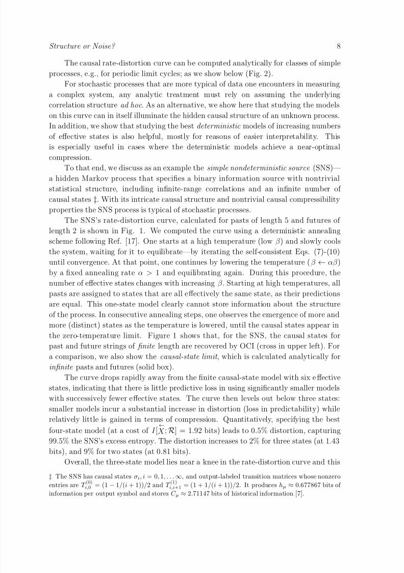
The causal rate-distortion curve can be computed analytically for classes of simple

processes, e.g., for periodic limit cycles; as we show below (Fig. 2).

For stochastic processes that are more typical of data one encounters in measuring

a complex system, any analytic treatment must rely on assuming the underlying

correlation structure ad hoc. As an alternative, we show here that studying the models

on this curve can in itself illuminate the hidden causal structure of an unknown process.

In addition, we show that studying the best deterministic models of increasing numbers

of eff ective states is also helpful, mostly for reasons of easier interpretability. This

is especially useful in cases where the deterministic models achieve a near-optimal

compression.

To that end, we discuss as an example the simple nondeterministic source (SNS)—

a hidden Markov process that specifies a binary information source with nontrivial

statistical structure, including infinite-range correlations and an infinite number of

causal states ‡. With its intricate causal structure and nontrivial causal compressibilityproperties the SNS process is typical of stochastic processes.

The SNS’s rate-distortion curve, calculated for pasts of length 5 and futures of

length 2 is shown in Fig. 1. We computed the curve using a deterministic annealing

scheme following Ref. [17]. One starts at a high temperature (low β) and slowly cools

the system, waiting for it to equilibrate—by iterating the self-consistent Eqs. (7)-(10)

until convergence. At that point, one continues by lowering the temperature (β ← αβ)

by a fixed annealing rate α > 1 and equilibrating again. During this procedure, the

number of eff ective states changes with increasing β. Starting at high temperatures, all

pasts are assigned to states that are all eff ectively the same state, as their predictions

are equal. This one-state model clearly cannot store information about the structureof the process. In consecutive annealing steps, one observes the emergence of more and

more (distinct) states as the temperature is lowered, until the causal states appear in

the zero-temperature limit. Figure 1 shows that, for the SNS, the causal states for

past and future strings of finite length are recovered by OCI (cross in upper left). For

a comparison, we also show the causal-state limit , which is calculated analytically for

infinite pasts and futures (solid box).

The curve drops rapidly away from the finite causal-state model with six eff ective

states, indicating that there is little predictive loss in using significantly smaller models

with successively fewer eff

ective states. The curve then levels out below three states:smaller models incur a substantial increase in distortion (loss in predictability) while

relatively little is gained in terms of compression. Quantitatively, specifying the best

four-state model (at a cost of I [←

X ;R] = 1.92 bits) leads to 0.5% distortion, capturing

99.5% the SNS’s excess entropy. The distortion increases to 2% for three states (at 1.43

bits), and 9% for two states (at 0.81 bits).

Overall, the three-state model lies near a knee in the rate-distortion curve and this

‡ The SNS has causal states σi, i = 0, 1, . . .∞, and output-labeled transition matrices whose nonzero

entries are T (0)i,0 = (1 − 1/(i + 1))/2 and T

(1)i,i+1 = (1 + 1/(i + 1))/2. It produces hµ ≈ 0.677867 bits of

information per output symbol and stores C µ ≈ 2.71147 bits of historical information [7].




suggests that it is a good compromise between model complexity and predictability.

The inset in Fig. 1 shows the reconstructed conditional future distributions for the

optimal three-state and six-state models in the simplex P(→

X 2

|←

x5). The six-state model

(crosses) reconstructs the true causal-state conditional future distributions (boxes),calculated from analytically known finite-sequence causal states. The figure illustrates

why the three-state model (circles) is a good compromise: two of the three-state model’s

conditional future distributions capture the two more-distinct SNS conditional future

distributions, and its third one summarizes the remaining, less diff erent, SNS conditional

future distributions.

The two-state model, however, already captures over 90% of the predictive

information, suggesting that a simple algorithm may be sufficient for characterizing the

complex statistical structure of the SNS. This two-state model is almost deterministic,

assigning those pasts which end on the symbol 0 to one state, and those which end on

the symbol 1 to the other state. The deterministic three-state model retains the clusterwith histories that end in 0, but assigns those histories which end in 01 to a diff erent

state than the ones that end in 11. Similarly, the deterministic four-state model splits

the 11 cluster into a state for histories ending in 011 and one for those ending in 111,

and so forth for increasingly large numbers of states. In conclusion, the hierarchy of OCI

models summarizes pasts in accordance to the most recent occurrence of the symbol 0.

5. Rate-Distortion Curves for IID and Predictively Reversible Processes

Other frequently studied processes include two classes of particular interest due to

their widespread use, for which the causal rate-distortion curve can be computed

analytically. On one extreme of randomness are the IID processes alluded to in

the introduction, such as the biased coin—by definition, a completely random and

unstructured source. For all IID processes, the rate-distortion curve collapses to

a single point at (0, 0), indicating that they are wholly unpredictable and causally

incompressible. This is easily seen by noting first that for IID processes the excess

entropy I [←

X ;→

X ] vanishes, since P(→

X |←

x) = P(→

X ). Therefore, I [←

X ;→

X |R] = 0, vanishes,

too §. Second, the energy function E (ρ,←

x) in the optimal assignments, Eq. (8), vanishes,

since P(→

X |ρ) = P(→

X |←

x)P(←X|ρ)= P(

→

X ). The optimal assignment given by Eq. (7) is

therefore the uniform distribution, and hence I [←

X ;R]|Popt= 0.

At the other extreme are the predictively reversible processes for which

P(→

x |←

x) = δ→x ,f (

←

x ), (11)

where f is bijective. Given that the future is a function of the past, these are the

zero entropy-rate processes. Periodic processes are in this class, as is the Morse-

Thue aperiodic process [20]. They have a rate-distortion curve that is a straight line,

the negative diagonal, running from [0,H [→

X ]] to [H [→

X ], 0]. To see this, note that

§ Since then I [←

X ;→

X |R] = −I [→

X ;R], which can only be true if both sides are 0.




I [←

X ;→

X ] = H [→

X ], due to Eq. (11). Furthermore, P(→

x) = P(←

x) and P(→

x |ρ) = P(←

x|ρ)

and, therefore, I [←

X ;→

X |R] = H [→

X ] − I [←

X ;R]. In this case, at each level of abstraction,

specifying the future to one bit higher accuracy costs us exactly one bit in model

complexity. Figure 2 illustrates the rate-distortion curves for both the IID and periodicpredictively reversible processes.

I [←

X ;R]

0

0 I [→

X ;←

X R]|

1 state

Feasible

1 state

E

C

Figure 2. Schematic illustration of the causal incompressibility of independent,

identically distributed processes (square) and predictively reversible processes (straight

line connecting circles) for the case when H [←

X ] and H [→

X ] are finite. These are the

periodic processes and we have C µ = H [←

X ] = logP and E = H [→

X ] = logP , where P

is the period. The dashed lines indicate the upper bounds: I [←

X ;→

X |R] ≤ I [

←

X ;→

X ] = E,

and I [←

X ;R] ≤ H [←

X ] = C µ.

The examples show how studying the hierarchy of optimal models, and the shape

of the associated rate-distortion curve, allows one to learn about a stochastic process’s

causal compressibility. The analysis reveals the causal structure of the underlying

process and demarcates the boundary between structure and noise.

6. Finite-Sample Fluctuations

As in statistical mechanics, so far we assumed that the distribution P(

←

X ,

→

X ) is given.And so, the above results bear on an intrinsic distinction between structure and noise

for a process, unsullied by statistical sample fluctuations.

However, when one builds a model from finite samples, then the distributions must

be estimated from the available data and so sample fluctuations must be taken into

account. Intuitively, limited data size sets a bound on how much we can consider to

be structure without overfitting. It turns out that using Ref. [21], the eff ects of finite

data can be corrected, as we show in Ref. [5]. This connects the approach taken here to

statistical inference and machine learning, where model complexity control is designed

to avoid overfitting due to finite-sample fluctuations; see, e.g, [22, 23, 24, 25, 26].




7. Conclusion

We showed how rate-distortion theory can be employed to find optimal causal models

at varying degrees of abstraction. Starting with the simple modeling principle of causal

shielding, an objective function was constructed that embodies the trade-off betweenmodel complexity and predictive power. Since the variational principle corresponds to

a rate-distortion theory, known analysis methods could be employed. In particular, we

showed how the method maps onto the known information bottleneck method, and we

pointed out that it finds the causal-state partition exactly when the constraint on model

complexity is relaxed. This gives a physical grounding to this inference method.

Furthermore, we gave a procedure to automatically build predictive models with

desired degrees of abstraction: Solutions to the objective function are found using

an iterative algorithm, and the rate-distortion curve is computed using deterministic

annealing. For certain processes we calculated the curve analytically. These anda numerical example served to demonstrate how its shape reveals a process’s causal

compressibility, providing direct guidance for automated model making. In particular,

we showed how a model distinguishes between what it eff ectively considers to be

underlying structure and what is noise. Practically speaking, natural processes that have

high causal compressibility will admit particularly parsimonious theories that capture a

large fraction of observed behavior.

By focusing on the case in which limitations due to finite sampling errors are absent,

we emphasized that compact representations, in and of themselves, are critical aids to

scientific understanding. We pointed out, however, that finite data set size imposes a

maximum level of allowable accuracy before overfitting occurs and that previous resultscan be used to find that demarcation line as well.

Acknowledgments

We thank Chris Ellison (supported on a GAANN fellowship) and Joerg Reichardt for

programming and discussions. S. Still thanks William Bialek for countless enlightening

conversations. The CSC Network Dynamics Program funded by Intel Corporation

supported part of this work. It was also partially supported by the DARPA Physical

Intelligence Program.




[1] W. von Rueden and R. Mondardini. The Large Hadron Collider (LHC) data challenge. Technical

report, IEEE Technical Committee on Scalable Computing, 2007. http://www.ieeetcsc.org/

newsletters/2003-01/mondardini.html.

[2] Anonymous. LSST observatory—Baseline configuration. Technical report, LSST Corporation,

Tucson, AZ, 2007. http://www.lsst.org/Science/lsst_baseline.shtml.[3] Anonymous. NIST 2006 machine translation evaluation official results. Technical report, National

Institute of Standards and Technologies, Washington, DC, 2006.

[4] M. E. J. Newman. The structure of scientific collaboration networks. Proc. Natl. Acad. Sci. USA,

78(2):404–409, 2001.

[5] S. Still, J. P. Crutchfield, and C. Ellison. Optimal causal inference: Estimating stored information

and approximating causal architecture. CHAOS, Special Issue on Intrinsic and Designed

Computation: Information Processing in Dynamical Systems, page in press, September 2010.

Original version (2007) available at arXiv: 0708.1580.

[6] N. Tishby, F. Pereira, and W. Bialek. The information bottleneck method. In B. Hajek and R. S.

Sreenivas, editors, Proc. 37th Allerton Conference, pages 368–377. University of Illinois, 1999.

[7] J. P. Crutchfield and K. Young. Inferring statistical complexity. Phys. Rev. Let., 63:105–108,

1989. J. P. Crutchfield. The Calculi of Emergence: Computation, Dynamics, and Induction.Physica D , 75:11-54, 1994. J. P. Crutchfield and C. R. Shalizi. Thermodynamic Depth of Causal

States: Objective Complexity via Minimal Representations. Phys. Rev. E , 59(1):275-283, 1999.

[8] William of Ockham. Philosophical Writings: A Selection, Translated, with an Introduction, by

Philotheus Boehner, O.F.M., Late Professor of Philosophy, The Franciscan Institute . Bobbs-

Merrill, Indianapolis, 1964. first pub. various European cities, early 1300s.

[9] P. Domingos. The role of Occam’s Razor in knowledge discovery. Data Mining and Knowledge

Discovery , 3:409–425, 1999.

[10] M. Casdagli and S. Eubank, editors. Nonlinear Modeling , SFI Studies in the Sciences of

Complexity, Reading, Massachusetts, 1992. Addison-Wesley.

[11] J. C. Sprott. Chaos and Time-Series Analysis. Oxford University Press, Oxford, UK, second

edition, 2003.

[12] H. Kantz and T. Schreiber. Nonlinear Time Series Analysis. Cambridge University Press,Cambridge, UK, second edition, 2006.

[13] J. P. Crutchfield and B. S. McNamara. Equations of motion from a data series. Complex Systems,

1:417 – 452, 1987.

[14] T. M. Cover and J. A. Thomas. Elements of Information Theory . Wiley-Interscience, New York,

second edition, 2006.

[15] W. Bialek, I. Nemenman, and N. Tishby. Predictability, Complexity and Learning. Neural

Computation , 13:2409–2463, 2001.

[16] C. E. Shannon. A mathematical theory of communication. Bell Sys. Tech. J., 27, 1948. Reprinted

in C. E. Shannon and W. Weaver The Mathematical Theory of Communication , University of

Illinois Press, Urbana, 1949.

[17] K. Rose. Deterministic Annealing for Clustering, Compression, Classification, Regression, and

Related Optimization Problems. Proc. IEEE , 86(11):2210–2239, 1998.[18] R. E. Blahut. Computation of channel capacity and rate distortion function. IEEE Transactions

on Information Theory IT-18 , pages 460–473, 1972.

[19] S. Arimoto. An algorithm for computing the capacity of arbitrary discrete memoryless channels.

IEEE Transactions on Information Theory IT-18 , pages 14–20, 1972.

[20] J. P. Crutchfield and D. P. Feldman. Regularities unseen, randomness observed: Levels of entropy

convergence. CHAOS , 13(1):25–54, 2003.

[21] S. Still and W. Bialek. How many clusters? An information theoretic perspective. Neural

Computation , 16(12):2483–2506, 2004.

[22] C. Wallace and D. Boulton. An information measure for classification. Comput. J., 11:185, 1968.

[23] H. Akaike. An objective use of Bayesian models. Ann. Inst. Statist. Math., 29A:9, 1977.




[24] J. Rissanen. Stochastic Complexity in Statistical Inquiry . World Scientific, Singapore, 1989.

[25] V. Vapnik. The Nature of Statistical Learning Theory . Springer Verlag, New York, 1995.

[26] D. MacKay. Information Theory, Inference, and Learning Algorithms. Cambridge University

Press, Cambridge, 2003.

Documents

Structure or Noise? Susanne Still