STRUCTURE-FROM-MOTION FOR SYSTEMS WITH PERSPECTIVE

AND OMNIDIRECTIONAL CAMERAS

YALIN BASTANLAR

JULY 2009

STRUCTURE-FROM-MOTION FOR SYSTEMS WITH PERSPECTIVE AND

OMNIDIRECTIONAL CAMERAS

A THESIS SUBMITTED TO

THE GRADUATE SCHOOL OF INFORMATICS

OF

MIDDLE EAST TECHNICAL UNIVERSITY

BY

YALIN BASTANLAR

IN PARTIAL FULFILLMENT OF THE REQUIREMENTS FOR THE DEGREE OF

DOCTOR OF PHILOSOPHY

IN

THE DEPARTMENT OF INFORMATION SYSTEMS

JULY 2009

Approval of the Graduate School of Informatics:

Prof. Dr. Nazife BAYKAL

Director

I certify that this thesis satisfies all the requirements as a thesis for the degree

of Doctor of Philosophy.

Prof. Dr. Yasemin YARDIMCI

Head of Department

This is to certify that we have read this thesis and that in our opinion it is fully

adequate in scope and quality as a thesis for the degree of Doctor of Philosophy.

Asst. Prof. Dr. Alptekin TEMIZEL Prof. Dr. Yasemin YARDIMCI

Co-Supervisor Supervisor

Examining Committee Members

Assoc. Prof. Dr. Aydın ALATAN (METU, EEE)

Prof. Dr. Yasemin YARDIMCI (METU, II)

Asst. Prof. Dr. Alptekin TEMIZEL (METU, II)

Assoc. Prof. Dr. Ugur GUDUKBAY (Bilkent Univ., CS)

Asst. Prof. Dr. Altan KOCYIGIT (METU, II)

I hereby declare that all information in this document has been

obtained and presented in accordance with academic rules and ethical

conduct. I also declare that, as required by these rules and conduct,

I have fully cited and referenced all materials and results that are not

original to this work.

Name, Last name : Yalın Bastanlar

Signature :

iii

abstract

STRUCTURE-FROM-MOTION FOR SYSTEMS WITH

PERSPECTIVE AND OMNIDIRECTIONAL CAMERAS

BASTANLAR, Yalın

Ph.D., Department of Information Systems

Supervisor: Prof. Dr. Yasemin YARDIMCI

July 2009, 100 pages

In this thesis, a pipeline for structure-from-motion with mixed camera types

is described and methods for the steps of this pipeline to make it effective and

automatic are proposed. These steps can be summarized as calibration, feature

point matching, epipolar geometry and pose estimation, triangulation and bundle

adjustment. We worked with catadioptric omnidirectional and perspective cam-

eras and employed the sphere camera model, which encompasses single-viewpoint

catadioptric systems as well as perspective cameras.

For calibration of the sphere camera model, a new technique that has the

advantage of linear and automatic parameter initialization is proposed. The

projection of 3D points on a catadioptric image is represented linearly with a 6×10

projection matrix using lifted coordinates. This projection matrix is computed

with an adequate number of 3D-2D correspondences and decomposed to obtain

intrinsic and extrinsic parameters. Then, a non-linear optimization is performed

to refine the parameters.

For feature point matching between hybrid camera images, scale invariant fea-

ture transform (SIFT) is employed and a method is proposed to improve the SIFT

iv

matching output. With the proposed approach, omnidirectional-perspective match-

ing performance significantly increases to enable automatic point matching. In

addition, the use of virtual camera plane (VCP) images is evaluated, which are

perspective images produced by unwarping the corresponding region in the om-

nidirectional image.

The hybrid epipolar geometry is estimated using random sample consensus

(RANSAC) and alternatives of pose estimation methods are evaluated. A weight-

ing strategy for iterative linear triangulation which improves the structure esti-

mation accuracy is proposed. Finally, multi-view structure-from-motion (SfM) is

performed by employing the approach of adding views to the structure one by one.

To refine the structure estimated with multiple views, sparse bundle adjustment

method is employed with a modification to use the sphere camera model.

Experiments on simulated and real images for the proposed approaches are

conducted. Also, the results of hybrid multi-view SfM with real images are

demonstrated, emphasizing the cases where it is advantageous to use omnidi-

rectional cameras with perspective cameras.

Keywords: Catadioptric omnidirectional camera, mixed camera system, camera

calibration, feature point matching, structure-from-motion.

v

oz

PERSPEKTIF VE TUMYONLU KAMERA KULLANAN

SISTEMLER ILE HAREKETTEN YAPI CIKARIMI

BASTANLAR, Yalın

Doktora, Bilisim Sistemleri Bolumu

Tez Yoneticisi: Prof. Dr. Yasemin YARDIMCI

Temmuz 2009, 100 sayfa

Bu tezde, karma kameralı sistemler ile hareketten yapı cıkarımı yapmak icin

basamaklı bir sema tanımlanmıs ve bu basamaklar icin yontemler gelistirilerek

yapı cıkarımı isleminin daha gurbuz ve otomatik olması saglanmıstır. Tanımlanan

basamaklar, kamera kalibrasyonu, nokta eslestirme, epipolar geometri ve kam-

eraların durus (konum ve yonelim) kestirimi, ucgenleme ve toplu duzenleme

olarak ozetlenebilir. Katadioptrik tumyonlu kameralar ve perspektif kameralar

ile calıstık ve hem tek gorus noktalı (single viewpoint) tumyonlu kameraları hem

de perspektif kameraları kapsayan kuresel kamera modelini kullandık.

Kuresel kamera modelinin kalibrasyonu icin dogrusal ve otomatik parametre

ilklendirmesi avantajına sahip yeni bir yontem gelistirilmistir. 3B uzaydaki nok-

taların katadioptrik imgeye dusurulmesi, yukseltilmis koordinatlar kullanılarak,

6× 10 boyutunda bir izdusum matrisi ile dogrusal olarak ifade edilmistir. Yeterli

sayıda 3B-2B nokta eslenigi ile bu izdusum matrisi hesaplanabilmekte, icsel ve

dıssal parametreler bu matristen elde edilebilmektedir. Ardından dogrusal ol-

mayan bir optimizasyon ile parametreler iyilestirilmektedir.

Karma kamera imgeleri arasında nokta eslemesi icin, olcekten bagımsız oznitelik

vi

donusumu (SIFT) kullanılmıs ve esleme basarısını artırmak uzere bir yontem

onerilmistir. Onerilen yontemle tumyonlu-perspektif esleme performansı otomatik

eslemeyi mumkun kılacak olcude artmıstır. Ayrıca, tumyonlu imgelerden bukme

sonucu elde edilen ve perspektif imge ozellikleri tasıyan sanal kamera duzlemi

(VCP) goruntulerini kullanarak esleme yapılması da arastırılmıstır.

Karma epipolar geometri kestirimi rasgele ornek onaylasımı (RANSAC) ile

gerceklenmis ve kamera durus (konum ve yonelim) tespiti icin alternatifler degerlen-

dirilmistir. Yapı kestirimi dogrulugunu artırmak uzere dongulu dogrusal ucgenleme

icin bir agırlıklandırma yontemi gelistirilmistir. Son olarak, cok imgeli hareketten

yapı cıkarımı icin, yapıya her defasında yeni bir imge ekleme yaklasımına dayalı

yontem uygulanmıs ve kestirilen yapının dogrulugunun artırılması icin nadir verili

toplu duzenleme (sparse bundle adjustment) yontemi kuresel kamera modeli icin

modifiye edilerek kullanılmıstır.

Onerilen yontemler icin benzetimli ve gercek imgeler uzerinde deneyler yapıl-

mıstır. Ayrıca, perspektif kameralarla beraber tumyonlu kameraları kullanmanın

avantajlı oldugu durumlar vurgulanarak, karma kameralarla cok imgeli hareketten

yapı cıkarımı gosterimleri yapılmıstır.

Anahtar Kelimeler: Katadioptrik tumyonlu kamera, karma kameralı sistemler,

kamera kalibrasyonu, nokta esleme, hareketten yapı cıkarımı.

vii

acknowledgements

I would like to express my sincere gratitude to Prof. Dr. Yasemin Yardımcı

for her valuable supervision and friendly attitute throughout the research. Her

guidance positively influenced my academic activities and I have been able to

complete this thesis.

I have conducted some of my studies in INRIA Rhone-Alpes with Prof. Peter

Sturm. I would like to thank him for this precious support. It is a pleasure to

work with him.

I wish to thank Asst. Prof. Dr. Alptekin Temizel, Assoc. Prof. Dr. Aydın

Alatan and Asst. Prof. Dr. Erhan Eren for their advises concerning the research

held in this thesis. I also thank Assoc. Prof. Dr. Ugur Gudukbay and Asst.

Prof. Dr. Altan Kocyigit for reviewing this work.

I would like to express my deepest gratitude to my family for their uncondi-

tional support during my life. Special thanks goes to my beloved girlfriend Evren

for her continuous support and understanding. Finally, I would like to thank

my colleagues Luis, Mustafa, Koray, Habil and Medeni for helping me in various

ways.

This thesis work is supported by The Scientific and Technical Research Coun-

cil of Turkey (TUBITAK) under the grant EEEAG-105E187 and with the re-

searcher support programs 2211 and 2214.

viii

table of contents

abstract . . . . . . . . . . . . . . . . . . . . . . . . . . . . . . . . . . . . . . . . . . . . . . . . . . . iv

oz . . . . . . . . . . . . . . . . . . . . . . . . . . . . . . . . . . . . . . . . . . . . . . . . . . . . . . . . . . . vi

acknowledgments . . . . . . . . . . . . . . . . . . . . . . . . . . . . . . . . . . . . . . . . viii

table of contents . . . . . . . . . . . . . . . . . . . . . . . . . . . . . . . . . . . . . . . . ix

list of tables . . . . . . . . . . . . . . . . . . . . . . . . . . . . . . . . . . . . . . . . . . . . . xii

list of figures . . . . . . . . . . . . . . . . . . . . . . . . . . . . . . . . . . . . . . . . . . . . xiv

CHAPTER

1 introduction . . . . . . . . . . . . . . . . . . . . . . . . . . . . . . . . . . . . . . . . . . . 1

1.1 Motivation . . . . . . . . . . . . . . . . . . . . . . . . . . . . . . . 1

1.2 Previous Work on Hybrid Systems . . . . . . . . . . . . . . . . . . 2

1.3 Thesis Study . . . . . . . . . . . . . . . . . . . . . . . . . . . . . 3

1.4 Contributions of the Thesis . . . . . . . . . . . . . . . . . . . . . 5

1.5 Road Map . . . . . . . . . . . . . . . . . . . . . . . . . . . . . . . 6

2 Background on Omnidirectional Imaging . . . . . . . . . . 7

2.1 Introduction to Omnidirectional Vision . . . . . . . . . . . . . . . 7

2.1.1 Single-viewpoint Property . . . . . . . . . . . . . . . . . . 8

2.1.2 Fish-eye Lenses . . . . . . . . . . . . . . . . . . . . . . . . 9

2.2 Sphere Camera Model . . . . . . . . . . . . . . . . . . . . . . . . 11

2.2.1 Relation between the Real Catadioptric System and the

Sphere Camera Model . . . . . . . . . . . . . . . . . . . . 13

ix

3 DLT-Based Calibration of Sphere Camera Model 16

3.1 Literature on Catadioptric Camera Calibration . . . . . . . . . . . 16

3.2 Proposed Calibration Technique . . . . . . . . . . . . . . . . . . . 17

3.2.1 Mathematical Background on Coordinate Lifting . . . . . 17

3.2.2 Generic Projection Matrix . . . . . . . . . . . . . . . . . . 19

3.2.3 Computation of the Generic Projection Matrix . . . . . . . 20

3.2.4 Decomposition of the Generic Projection Matrix . . . . . . 21

3.2.5 Other Parameters of Non-linear Calibration . . . . . . . . 22

3.3 Calibration Experiments in a Simulated Environment . . . . . . . 24

3.3.1 Estimation Errors for Different Camera Types . . . . . . . 25

3.3.2 Tilting and Distortion . . . . . . . . . . . . . . . . . . . . 27

3.4 Calibration with Real Images using a 3D Pattern . . . . . . . . . 29

3.5 Conclusions . . . . . . . . . . . . . . . . . . . . . . . . . . . . . . 31

4 Feature Matching . . . . . . . . . . . . . . . . . . . . . . . . . . . . . . . . . . . . . 32

4.1 Improving the Initial SIFT Output . . . . . . . . . . . . . . . . . 32

4.1.1 Preprocessing Perspective Image . . . . . . . . . . . . . . . 34

4.1.2 Final Elimination . . . . . . . . . . . . . . . . . . . . . . . 38

4.2 Creating Virtual Camera Plane Images . . . . . . . . . . . . . . . 40

4.3 Experiments . . . . . . . . . . . . . . . . . . . . . . . . . . . . . . 41

4.3.1 Experiments with Catadioptric Cameras . . . . . . . . . . 41

4.3.2 Experiments with Fish-eye Camera . . . . . . . . . . . . . 46

4.4 Conclusions . . . . . . . . . . . . . . . . . . . . . . . . . . . . . . 52

5 Robust Epipolar Geometry and Pose Estimation . 55

5.1 Hybrid Epipolar Geometry . . . . . . . . . . . . . . . . . . . . . . 55

5.2 Robust Epipolar Geometry Estimation . . . . . . . . . . . . . . . 57

5.2.1 Linear Estimation of Fundamental Matrix . . . . . . . . . 58

5.2.2 Normalization of Point Coordinates . . . . . . . . . . . . . 59

5.2.3 Distance Threshold . . . . . . . . . . . . . . . . . . . . . . 62

5.2.4 Applying Rank-2 Constraint . . . . . . . . . . . . . . . . . 63

5.3 Experiments of Outlier Elimination . . . . . . . . . . . . . . . . . 64

x

5.4 Pose Estimation . . . . . . . . . . . . . . . . . . . . . . . . . . . . 65

5.5 Conclusions . . . . . . . . . . . . . . . . . . . . . . . . . . . . . . 67

6 Triangulation . . . . . . . . . . . . . . . . . . . . . . . . . . . . . . . . . . . . . . . . . . 69

6.1 Weighted Triangulation for Mixed Camera Images . . . . . . . . . 69

6.2 Experiments . . . . . . . . . . . . . . . . . . . . . . . . . . . . . . 72

6.3 Structure-from-Motion with Real Images . . . . . . . . . . . . . . 75

6.4 Conclusions . . . . . . . . . . . . . . . . . . . . . . . . . . . . . . 76

7 Multi-view SfM . . . . . . . . . . . . . . . . . . . . . . . . . . . . . . . . . . . . . . . . 78

7.1 Computing the Projection Matrices of Additional Views . . . . . 78

7.2 Sparse Bundle Adjustment . . . . . . . . . . . . . . . . . . . . . . 81

7.2.1 Experiment . . . . . . . . . . . . . . . . . . . . . . . . . . 81

7.3 Merging 3D Structures of Different Hybrid Image Pairs . . . . . . 82

7.3.1 Experiment . . . . . . . . . . . . . . . . . . . . . . . . . . 85

7.4 Conclusions . . . . . . . . . . . . . . . . . . . . . . . . . . . . . . 85

8 Conclusions . . . . . . . . . . . . . . . . . . . . . . . . . . . . . . . . . . . . . . . . . . . . 88

8.1 Limitations and Future Work . . . . . . . . . . . . . . . . . . . . 91

references . . . . . . . . . . . . . . . . . . . . . . . . . . . . . . . . . . . . . . . . . . . . . . . . . 92

vita . . . . . . . . . . . . . . . . . . . . . . . . . . . . . . . . . . . . . . . . . . . . . . . . . . . . . . . . . 98

xi

list of tables

3.1 Calibration experiment with simulated images. Initial and opti-

mized estimates of parameters for varying grid heights and (ξ, f)

values. . . . . . . . . . . . . . . . . . . . . . . . . . . . . . . . . . 26

3.2 Initial values (DLT) and non-linear optimization estimates of in-

trinsic and extrinsic parameters for two different amounts of noise:

σ = 0.5 and σ = 1.0. . . . . . . . . . . . . . . . . . . . . . . . . . 27

3.3 Estimating tangential distortion with tilt parameters. σ = 0.5 pixels. 28

3.4 Intrinsic parameters estimated with the proposed calibration ap-

proach. . . . . . . . . . . . . . . . . . . . . . . . . . . . . . . . . . 30

4.1 Number of SIFT features detected in a catadioptric and perspec-

tive image pair (Pers2-Omni2). . . . . . . . . . . . . . . . . . . . 33

4.2 Comparison with Lowe’s proposal of elimination. Number of total

and true/false matches for the example hybrid image pair (Pers2

- Omni2). . . . . . . . . . . . . . . . . . . . . . . . . . . . . . . . 38

4.3 Matching results for the image pairs of indoor matching experi-

ment. True/false match ratios (T/F) after the initial and scale

restricted matching. . . . . . . . . . . . . . . . . . . . . . . . . . . 45

4.4 Matching results for the image pairs of outdoor matching exper-

iment. True/false match ratios (T/F) after the initial and scale

restricted matching. . . . . . . . . . . . . . . . . . . . . . . . . . . 48

4.5 Matching results for the fisheye-perspective matching experiment.

True/false match ratios (T/F) after the initial and scale restricted

matching. . . . . . . . . . . . . . . . . . . . . . . . . . . . . . . . 52

5.1 Entries of r for varying scale normalization factors, (nomni,npers). . 61

5.2 Median distance errors (in pixels) for different fundamental matri-

ces computed with varying number of points and scale normaliza-

tion values. . . . . . . . . . . . . . . . . . . . . . . . . . . . . . . 62

xii

5.3 Median distance errors to compare the two rank-2 imposition meth-

ods. . . . . . . . . . . . . . . . . . . . . . . . . . . . . . . . . . . 64

5.4 Matching results after RANSAC for hybrid image pairs (cf. Table

4.3). . . . . . . . . . . . . . . . . . . . . . . . . . . . . . . . . . . 65

5.5 Comparison of the two E-estimation methods: direct-E and E-from-F. 67

6.1 Results of triangulation experiments for the scene given in Fig. 6.2a. 73

6.2 Results of triangulation experiments for the scene given in Fig. 6.2b. 74

6.3 Distance estimate errors after triangulation for hybrid real image

pair. . . . . . . . . . . . . . . . . . . . . . . . . . . . . . . . . . . 76

7.1 The mean values of reprojection errors before and after SBA (in

pixels). . . . . . . . . . . . . . . . . . . . . . . . . . . . . . . . . . 82

xiii

list of figures

1.1 Steps of the implemented structure-from-motion pipeline. . . . . . 3

2.1 Directions of light rays in two single-viewpoint systems, (a) hyper-

catadioptric and (b) para-catadioptric. . . . . . . . . . . . . . . . 9

2.2 Directions of light rays in a non single-viewpoint system. . . . . . 10

2.3 Projection geometry of a fish-eye lens. . . . . . . . . . . . . . . . 11

2.4 Projection of a 3D point to two image points in sphere camera model. 12

2.5 Tilt in a real system (a) and in the sphere model (b). . . . . . . . 14

3.1 Block diagram of the proposed calibration technique. . . . . . . . 17

3.2 Examples of the simulated images with varying values of ξ, f and

vertical viewing angle (in degrees) of the highest point in 3D cali-

bration grid (θ). . . . . . . . . . . . . . . . . . . . . . . . . . . . . 25

3.3 Errors for ξ and f for increasing vertical viewing angle of the high-

est 3D pattern point (x-axis) after non-linear optimization. (a)

(ξ, f)=(0.96,360) (b) (ξ, f)=(0.80,270). . . . . . . . . . . . . . . . 27

3.4 (a) Omnidirectional image of the 3D pattern (1280×960 pixels,

flipped horizontal). (b) Constructed model of the 3D pattern. . . 29

3.5 Reprojections with the estimated parameters after initial (DLT)

step (a) and after non-linear optimization step (b). . . . . . . . . 30

4.1 Histogram of SR for the matches in the catadioptric-perspective

image pair given in Table 4.1. (a) SIFT applied on original image

pair, (b) SIFT applied on downsampled perspective image and

original catadioptric image. . . . . . . . . . . . . . . . . . . . . . 34

4.2 Matching results for the Pers2-Omni2 image pair with direct match-

ing resulted in 25/60 false/total match ratio (at the top) and with

the proposed preprocessing method resulted in 4/60 false/total

match ratio (at the bottom). . . . . . . . . . . . . . . . . . . . . . 35

xiv

4.3 Discrete time FFT before low-pass filtering (a) and after low-pass

filtering with σ = 2.5d/π where d = 3.6 (b). . . . . . . . . . . . . 36

4.4 Histogram of SR for the matches of the catadioptric-perspective

image pair given in Table 4.1 when Lowe’s elimination is applied. 37

4.5 Number of correct matches out of 60 matches for varying low-pass

filtering (σ) and downsampling (d) parameters for the example

mixed image pair (Table 4.1). . . . . . . . . . . . . . . . . . . . . 39

4.6 Generation of a virtual perspective image in a paraboloidal omni-

directional camera. . . . . . . . . . . . . . . . . . . . . . . . . . . 41

4.7 Locations and orientations of cameras in the indoor environment

catadioptric-perspective point matching experiment. . . . . . . . . 43

4.8 Images of point matching experiment, cameras are shown in Fig.

4.7. . . . . . . . . . . . . . . . . . . . . . . . . . . . . . . . . . . . 44

4.9 The true/total match ratios (in percentage) for Omni1-PersN (on

the left) and Omni2-PersN (on the right). . . . . . . . . . . . . . 45

4.10 Locations and orientations of the cameras in the outdoor environ-

ment catadioptric-perspective point matching experiment. . . . . 46

4.11 Images of 2nd point matching experiment, scene is shown in Fig.4.10. 47

4.12 The true/total match ratios (in percentage) of outdoor environ-

ment catadioptric-perspective point matching experiment (cf. Fig.

4.11 and Fig. 4.10). . . . . . . . . . . . . . . . . . . . . . . . . . . 48

4.13 Matching results for the Pers1-Omni1 pair in the outdoor experi-

ment (Table 4.4) with direct matching (top), preprocessed perspec-

tive - omnidirectional matching (middle) and preprocessed per-

spective - VCP matching (bottom). . . . . . . . . . . . . . . . . . 49

4.14 Fish-eye camera images of the point matching experiment: Fish1

(left) and Fish2 (right). The scene is given in Fig. 4.10. Fish1 and

Fish2 are at the same location with Omni1 and Omni2, respectively. 50

4.15 A perspective fish-eye hybrid image pair, where the common fea-

tures are not located at the central part of the fish-eye image but

closer to periphery. . . . . . . . . . . . . . . . . . . . . . . . . . . 50

xv

4.16 Matching results for the Pers2-Fish1 pair in the fish-eye experi-

ment (Table 4.5) with direct matching (top) and downsampling

approaches (bottom). . . . . . . . . . . . . . . . . . . . . . . . . . 51

4.17 The true/total match ratios (in percentage) of fisheye-perspective

point matching experiment (cf. Figs. 4.7 and 4.14). . . . . . . . . 51

5.1 Epipolar geometry between a perspective and a catadioptric image. 57

5.2 Example catadioptric-perspective pair and epipolar conics/lines of

point correspondences. . . . . . . . . . . . . . . . . . . . . . . . . 58

5.3 Simulation hybrid images for the normalization experiment. . . . 61

6.1 Depiction of doubling the focal length and decreasing the camera-

scene distance for triangulation on normalized rays, i.e. normalized

image plane. . . . . . . . . . . . . . . . . . . . . . . . . . . . . . . 71

6.2 Camera and grid positions in the scene of triangulation experiments. 73

6.3 Simulated hybrid image pair of the experiment in the first row of

Table 6.1. (a) perspective image, (b) omnidirectional image. . . . 74

6.4 Reconstruction with hybrid real image pair. Selected correspon-

dences on images are viewed on top. Images are cropped to make

points distinguishable. . . . . . . . . . . . . . . . . . . . . . . . . 77

7.1 Estimated camera positions, orientations and scene points for the

hybrid multi-view SfM experiment. (a) top-view (b) side-view. . . 82

7.2 Depiction of merging 3D structures estimated with different hybrid

image pairs. . . . . . . . . . . . . . . . . . . . . . . . . . . . . . . 83

7.3 Depiction of aligning and scaling the 2nd 3D structure w.r.t. the

first one to obtain a combined structure. . . . . . . . . . . . . . . 83

7.4 Matched points between the perspective images (top row) and

omnidirectional image (bottom-left) and the estimated structure

(bottom-right) for the experiment of merging 3D structures. . . . 86

xvi

chapter 1

introduction

1.1 Motivation

The 3D computer vision studies for omnidirectional cameras started about

a decade ago. Omnidirectional cameras provide 360 horizontal field of view

in a single image, which is an important advantage in many application areas

such as navigation, surveillance and 3D reconstruction [1–8]. With this enlarged

view, fewer omnidirectional cameras may substitute many perspective cameras.

Moreover, point correspondences from a variety of angles provide more stable

structure estimation [9] and degenerate cases like viewing only a planar surface are

avoided. Major drawback of these images is that they have lower resolution than

perspective images. Using perspective cameras together with omnidirectional

ones could improve the resolution while preserving the enlarged view advantage.

A possible scenario is 3D reconstruction in which omnidirectional cameras provide

low resolution background modeling whereas images of perspective cameras are

used for modeling foreground or specific objects. In such scenarios, since the

omnidirectional camera views a common scene with different perspective cameras

which do not have a common view in between, omnidirectional view is able to

combine the partial 3D structures obtained by different perspective cameras.

Considering surveillance applications, hybrid systems were proposed where

pan-tilt-zoom cameras are directed according to the information obtained by an

omnidirectional camera which performs event detection [4–6]. Such systems can

be enhanced by adding 3D structure and location estimation algorithms without

increasing the number of cameras.

While working with such hybrid camera systems, for consecutive steps of

structure-from-motion such as point matching, pose estimation, triangulation and

1

bundle adjustment, we need to modify the approaches that are used in systems

using one type of camera.

1.2 Previous Work on Hybrid Systems

Structure-from-motion (SfM) with perspective cameras have been studied for

a few decades and an extensive summary of algorithms can be found in [10]. For

omnidirectional cameras, SfM is performed by several researchers [9, 11–13] and

these studies include both calibrated and uncalibrated systems.

There are comparatively fewer studies on hybrid systems. Chen et al. [14]

worked on the exterior calibration of a perspective-catadioptric camera system.

They first calibrated the catadioptric camera, then using pre-measured 3D points

in the scene, they performed the exterior calibration of perspective cameras view-

ing the same scene. Adorni et al. [15] used a hybrid system for obstacle detection

problem in robot navigation. Chen and Yang [16] developed a region matching

algorithm for hybrid views based on planar homography.

Epipolar geometry between hybrid camera views was explained by Sturm [17]

for mixtures of paracatadioptric (catadioptric camera with a parabolic mirror)

and perspective cameras. Barreto and Daniilidis showed that the framework

can also be extended to cameras with lens distortion [18]. Recently, Sturm and

Barreto [19] extended these relations to the general catadioptric camera model,

which is valid for all central catadioptric cameras.

Puig et al. [20] worked on feature point matching and fundamental matrix es-

timation between perspective and catadioptric camera images. For point match-

ing, they first applied a catadioptric-to-panoramic conversion and directly applied

Scale Invariant Feature Transform (SIFT, [21]) between panoramic and perspec-

tive views. To eliminate the false matches they employed random sample con-

sensus (RANSAC, [22]) based on satisfying the epipolar constraint. They also

compared the representation capabilities of 3x4, 3x6 and 6x6 hybrid fundamental

matrices (with different coordinate lifting) for mirrors with varying parameters.

Ramalingam et al. [23] conducted a study on hybrid SfM. They used man-

ually selected feature point correspondences to estimate epipolar geometry and

mentioned that directly applying SIFT did not provide good results for their

fisheye-perspective image pairs. They employed midpoint method for triangu-

2

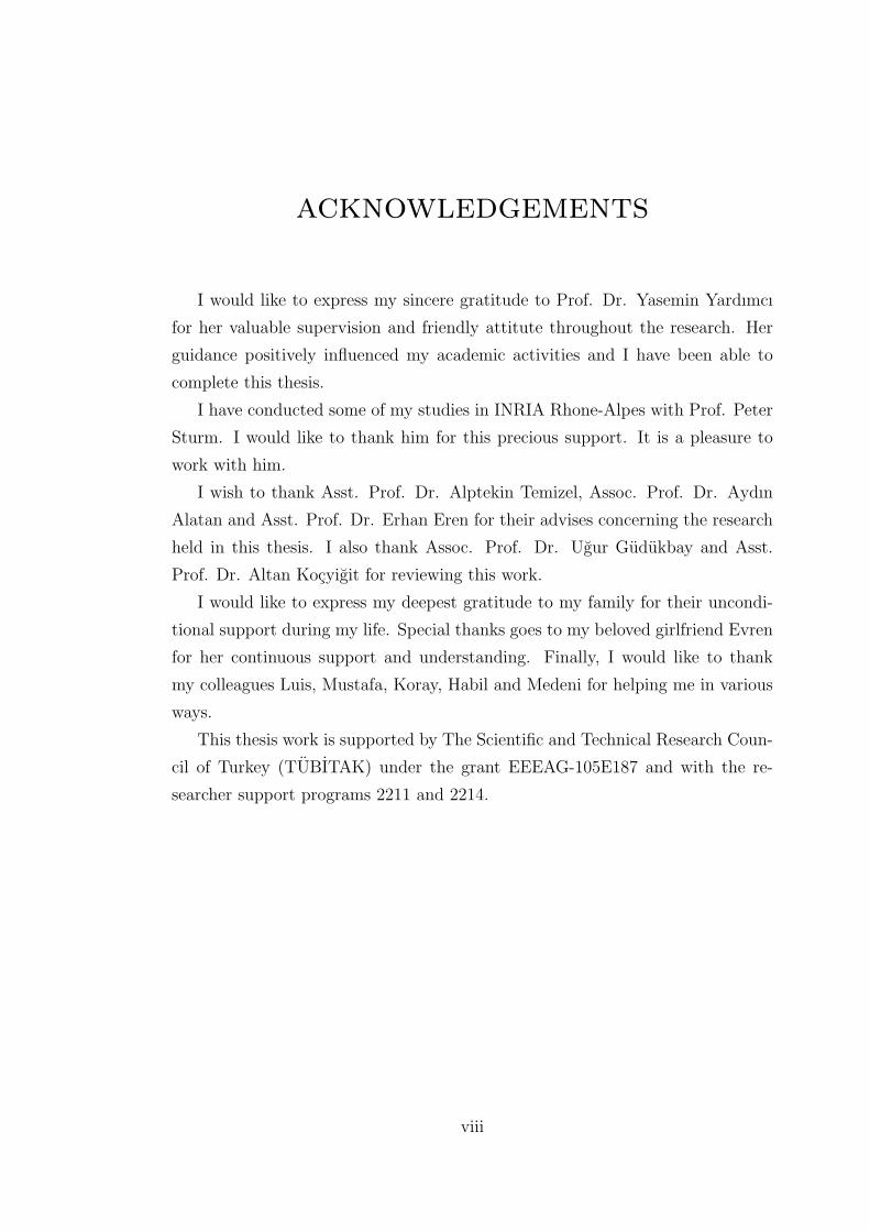
Figure 1.1: Steps of the implemented structure-from-motion pipeline.

lation to estimate 3D point coordinates and tested two different bundle adjust-

ment approaches, one minimizing the distances between projection rays and 3D

points and the other minimizing reprojection error. Their conclusion is that both

approaches are comparable to each other. They employed a highly generic non-

parametric imaging model, by which cameras are modeled with sets of projection

rays. Internal calibration of cameras was performed by the method given in [24].

In the next section, the scope of this thesis is explained and related to the

previous studies. Also, in the succeeding chapters, literature summaries regarding

the context of the present chapter are given.

1.3 Thesis Study

In this thesis, a pipeline for structure-from-motion with mixed camera types

is described and methods are proposed for the steps of this pipeline to make

it robust and automatic. These steps can be summarized as camera calibration,

point matching, epipolar geometry and pose estimation, triangulation and bundle

adjustment (Fig. 1.1).

To represent mixed types of cameras, we employ the sphere camera model [25]

3

which is able to cover single viewpoint catadioptric systems as well as perspective

cameras. Therefore, the SfM pipeline described here is generic for all the cameras

that can be modeled with the sphere model. Moreover, the proposed methods for

point matching and triangulation should work successfully also with the cameras

beyond the scope of the sphere camera model, since their applicability is not

related to the camera model.

The general imaging model used in [23] is more general than the sphere model

because it encompasses non-central catadioptric cameras as well. However, there

are some challenges such as defining a reprojection error for non-parametric model

since there is no analytical projection equation. Another disadvantage is that,

since the projection rays are represented with Plucker coordinates, the essential

matrix extends to a 6x6 matrix with a special form requiring 17 point correspon-

dences to be estimated linearly.

For calibration, we developed a calibration technique that is valid for all single-

viewpoint catadioptric cameras. We are able to represent the projection of 3D

points on a catadioptric image linearly with a 6x10 projection matrix, which uses

lifted coordinates for the image and 3D points. This projection matrix can be

computed with an adequate number of 3D-2D correspondences. We show how to

decompose it to obtain intrinsic and extrinsic parameters. Moreover, we use this

parameter estimation followed by a non-linear optimization to calibrate various

types of cameras. When compared to the alternative sphere model calibration

method [26], the proposed algorithm brings the advantage of linear and automatic

parameter initialization.

For feature matching between the images of different camera types, widely

accepted matching methods (eg. Scale Invariant Feature Transform: SIFT [21],

Maximally Stable Extremal Regions: MSER [27]) do not perform well when they

are directly employed for hybrid camera images [20,23]. In this thesis, we employ

SIFT to match feature points between omnidirectional and perspective images

and we propose a method to improve the SIFT matching result by preprocess-

ing the input images. We performed tests on both catadioptric and fish-eye

cameras and it is observed that, with the proposed approach, omnidirectional-

to-perspective matching performance significantly increases. We also evaluate

the use of virtual camera plane (VCP) images and observe that, for catadioptric

cameras, VCP-to-perspective matching is more robust to increasing baseline.

4

Computation of hybrid fundamental matrix (F) was previously explained [17,

18] and random sample consensus (RANSAC) was implemented for catadioptric-

perspective image pairs [20]. We define normalization matrices for lifted coordi-

nates so that normalization and denormalization can be performed linearly. We

present the results of our experiments on robust estimation of F to evaluate outlier

elimination and effect of normalization.

We compare two options for pose estimation (extraction of motion parame-

ters), one is directly estimating the essential matrix (E) with the calibrated 3D

rays, the other option is estimating hybrid F and then extracting E from it. We

performed experimental analysis to compare the effectiveness of these options.

For triangulation, we propose a weighting strategy for iterative linear-Eigen

triangulation method to improve its 3D location estimation accuracy when em-

ployed for hybrid image pairs. The only previous study including hybrid camera

triangulation was using the midpoint method [23]. However it has been shown

that iterative linear methods are superior to midpoint method and non-iterative

linear methods [28].

We perform multi-view SfM by employing the approach of adding views to

the structure one by one [29]. Sparse bundle adjustment method [30] has become

popular in the community due to its capability of solving enormous minimization

problems (with many cameras and 3D points) in a reasonable time. We employed

this method for multi-view hybrid SfM by modifying the projection function with

sphere model projection and intrinsic parameters with sphere model parameters.

We also demonstrate the complete hybrid multi-view SfM with real images

including the bundle adjustment step. We emphasize the case where the omnidi-

rectional camera is able to combine structures estimated with different perspective

cameras which do not have a view in common.

1.4 Contributions of the Thesis

• We developed a camera calibration technique for the sphere camera model.

Its advantage: Initialization of intrinsic parameters is performed linearly without

requiring a user input.

• We propose an improved feature point matching method which enables

automatic omnidirectional-perspective matching.

5

• We propose a weighting strategy for iterative linear-Eigen triangulation

method to improve its 3D structure estimation accuracy.

•We modified and tested existing approaches for hybrid SfM: Normalization,

Pose estimation, Multi-view SfM, Sparse bundle adjustment.

1.5 Road Map

Chapter 2 provides background information on omnidirectional vision. After

giving an introduction to omnidirectional vision and catadioptric cameras, sphere

camera model is introduced to the reader, which is the model we employ to

represent our hybrid cameras.

Chapter 3 begins with the literature survey on catadioptric camera calibration.

Then, it presents the details of the developed calibration method for the sphere

camera model together with the experiment results.

Chapter 4 presents the proposed feature point matching algorithm for mixed

camera images. It first explains why SIFT is not effective when applied directly

and how we solve the problem. Then the results of experiments with real images

of catadioptric and fish-eye cameras are presented.

Chapter 5 focuses on the epipolar geometry and pose estimation steps of the

SfM pipeline. The implementation of RANSAC on hybrid epipolar geometry and

normalization of lifted coordinates are explained. Moreover, the experimental

comparison of the options for pose estimation (extraction of motion parameters)

is given.

Chapter 6 presents the proposed weighting strategy for iterative linear-Eigen

triangulation method and shows its effectiveness to increase the 3D structure

estimation performance with simulated images. Also, a two-view hybrid SfM

experiment is presented in this chapter in order to evaluate the proposed trian-

gulation approach.

Chapter 7 gives the details of the work on multi-view SfM with hybrid images.

The improvement gained by sparse bundle adjustment is also given in this chapter.

The proof of concept given in this thesis is presented with experiments where the

complete pipeline of hybrid SfM is realized.

Finally, Chapter 8 presents conclusions and suggests future works.

6

chapter 2

Background on

Omnidirectional Imaging

In this chapter, we introduce the omnidirectional vision to the reader and

briefly explain image formation in catadioptric omnidirectional cameras, which

will serve as a background information for the following chapters. We also ex-

plain the sphere camera model (Section 2.2) which is able to represent all single-

viewpoint catadioptric cameras.

2.1 Introduction to Omnidirectional Vision

The term “omnidirectional” is used for the cameras that have very large fields

of view. An omnidirectional viewing device ideally has the capability of viewing

360 in all directions. It is not practical to produce a “true” omnidirectional sen-

sor, therefore manufactured cameras usually provide 360 horizontal view and a

sufficient field of vertical view. Fish-eye lenses also have extended field of views up

to a hemisphere and are used for omnidirectional viewing. However, most of the

omnidirectional cameras are catadioptric systems which means they use combina-

tions of mirrors and lenses. The term “catadioptrics” comprises “catoptrics”; the

science of reflecting surfaces (mirrors) and “dioptrics”; the science of refracting

elements (lenses). Rees [31] is the first to patent a catadioptric omnidirectional

capturing system using a hyperboloidal mirror and a normal perspective camera

in 1970. Since then, considerable amount of effort have been spent on the design

of mirrors with enlarged vertical field of views, low cost and varying resolution

properties. Among them, Nayar and Peri [32] worked on folded mirror systems

that use multiple mirrors in order to obtain smaller omnidirectional devices with

wider views. Conroy and Moore [33] derived mirror surfaces that are resolution

invariant vertically, so that adjacent pixels in omnidirectional image correspond

7

to the real world points that are vertically equi-distant from each other. In that

paper, stereo omnidirectional systems are also introduced. They are constructed

by two coaxial, axially symmetric mirror profiles. Hicks and Bajcsy [34] exhibited

a mirror design that views wide horizontal area under the mirror and reflects an

undistorted (perspective) omnidirectional image of this area. Gaspar et al. [35]

summarizes the constant horizontal, vertical and angular resolution issues and

presents a mirror that achieves uniform resolution when used with a specific log-

polar camera. Swaminathan et al. [36] discusses the design issues of mirrors that

minimize image errors.

2.1.1 Single-viewpoint Property

Catadioptric systems, combinations of camera lenses and mirrors, are able

to provide single-viewpoint property if the mirror has a focal point which can

behave like an effective pinhole. For instance, in the mirror shown in Fig. 2.1a,

light rays coming from the world points A, B and C and targeting the focal

point (single viewpoint) of the hyperboloidal mirror are reflected on the mirror

surface so that they will pass through the pinhole (camera center). This single

viewpoint acts a virtual pinhole through which the scene is viewed as in regular

perspective cameras. Paraboloidal mirrors also have single-viewpoint property,

but the rays targeting that viewpoint are reflected orthogonally, which requires

the use of a telecentric lens to collect the parallel rays (Figure 2.1b). Single

viewpoint constraint provides quick conversion of geometrically correct panoramic

and perspective images because they are generated as seen from the mentioned

viewpoint.

Since the cross sectional profiles of the mirrors of catadioptric sensors do not

change when rotated around the optical axis, the cross sections of the mirrors

are shown in the figures. Usually mirrors are referred with the names of these

2D cross-sections such as parabolic and hyperbolic mirrors. Catadioptric systems

are often referred with the associated mirror type such as para-catadioptric or

hyper-catadioptric systems.

For the system shown in Fig. 2.2, directions of the light rays that are used

for image formation do not intersect at a certain point as in the single-viewpoint

case, therefore a single point through which the scene can be viewed cannot be

8

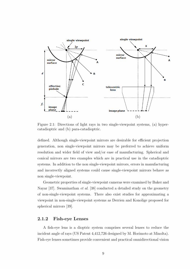
(a) (b)

Figure 2.1: Directions of light rays in two single-viewpoint systems, (a) hyper-catadioptric and (b) para-catadioptric.

defined. Although single-viewpoint mirrors are desirable for efficient projection

generation, non single-viewpoint mirrors may be preferred to achieve uniform

resolution and wider field of view and/or ease of manufacturing. Spherical and

conical mirrors are two examples which are in practical use in the catadioptric

systems. In addition to the non single-viewpoint mirrors, errors in manufacturing

and incorrectly aligned systems could cause single-viewpoint mirrors behave as

non single-viewpoint.

Geometric properties of single-viewpoint cameras were examined by Baker and

Nayar [37]. Swaminathan et al. [38] conducted a detailed study on the geometry

of non-single-viewpoint systems. There also exist studies for approximating a

viewpoint in non-single-viewpoint systems as Derrien and Konolige proposed for

spherical mirrors [39].

2.1.2 Fish-eye Lenses

A fish-eye lens is a dioptric system comprises several lenses to reduce the

incident angle of rays (US Patent 4,412,726 designed by M. Horimoto at Minolta).

Fish-eye lenses sometimes provide convenient and practical omnidirectional vision

9

Figure 2.2: Directions of light rays in a non single-viewpoint system.

for computer vision applications. Fig. 2.3 shows the projection geometry of a

fish-eye lens. Light rays passing through the adjacent pixels in the image belong

to the diverging rays coming from outside. With this ability, a lens can capture

more than a hemisphere (Eg. Fujinon Fisheye 185, FE185C046HA-1).

Fish-eye lenses belong to the non single-viewpoint family. A simple and com-

mon way to model the projection of these lenses is employing equi-distance pro-

jection model. It preserves equal distances in image plane for equal vertical angles

between the diverging light rays:

r = fθ

where θ is the angle between the optical axis and the incoming light ray, r is the

distance between the image point and the principal point and f is the focal length.

However, produced lenses do not exactly conform to the model and for accurate

calibration polynomial models are used to map image pixels (r) to the incoming

light rays (θ). Ho et al. [40] gives more information about history and physics

of fisheye lenses. They also present their test results with different projection

models.

10

Figure 2.3: Projection geometry of a fish-eye lens.

2.2 Sphere Camera Model

Now, we briefly explain the sphere model for catadioptric projection intro-

duced by Geyer and Daniilidis [25]. Later, Barreto and Daniilidis [18] showed

that the framework can also be extended to cameras with lens distortions. In

the following, matrices are represented by symbols in sans serif font, e.g. M and

vectors by bold symbols, e.g. Q, q. Equality of matrices or vectors up to a scalar

factor is written as ∼.

According to this model, all central catadioptric cameras can be modeled by

a unit sphere and a perspective camera, such that the projection of 3D points can

be performed in two steps (Fig. 2.2). First one is the projection of point Q in

3D space onto a unitary sphere and second one is the projection from the sphere

to the image plane. First projection gives rise to two intersection points on the

sphere, r±. The one that is visible to us is r+ and its projection on the image plane

is q+. This model covers all central catadioptric cameras, denoted by ξ, which

is the distance between the camera center and the center of the sphere. ξ = 0

for perspective, ξ = 1 for para-catadioptric, 0 < ξ < 1 for hyper-catadioptric

cameras.

Let the unit sphere be located at the origin and the optical center of the

perspective camera be located at the point Cp = (0, 0,−ξ)T making z-axis positive

downwards. The perspective projection from the sphere to the image plane is

11

Figure 2.4: Projection of a 3D point to two image points in sphere camera model.Camera is looking down, accordingly z-axis of the camera coordinate system ispositive downwards.

modeled by the projection matrix P ∼ K(I −Cp

), where K is the calibration

matrix of perspective camera embedded in the sphere model. To explain the

projection in detail, let the intersection point of the sphere and the line joining

its center and Q be

r+ =

(Q1, Q2, Q3,

√Q2

1 +Q22 +Q2

3

)T

in 4-vector homogeneous coordinates. The same point represented with respect

to the camera center, Cp, in non-homogeneous coordinates is

b+ =

(Q1, Q2, Q3 + ξ

√Q2

1 +Q22 +Q2

3

)T

Then, the image of the point in the perspective camera is

q+ ∼ Kb+ ∼ K

Q1

Q2

Q3 + ξ√Q2

1 +Q22 +Q2

3

(2.1)

Therefore, intrinsic parameters of this model are ξ and K. Please note that

in this formulation no rotation is modeled between sphere axis and perspective

camera inside. This fact is referred as tilting and discussed in Section 2.2.1 where

we also give the relation between the focal length of the sphere model and the

actual camera focal length.

12

Back-projection.

Computing the outgoing 3D ray corresponding to an image point can be per-

formed in two steps. First step is obtaining b from q and similar to any per-

spective camera it is computed by b = K−1q. Second step is carrying back the

origin of coordinate system from the camera center to the center of the sphere,

i.e. passing from b to r. Let (x, y, z) represent the 3D ray b, then the sphere

centered 3D ray, r, can be computed with the below equation [41]:

r =

zξ+√z2+(1−ξ2)(x2+y2)

x2+y2+z2x

zξ+√z2+(1−ξ2)(x2+y2)

x2+y2+z2y

zξ+√z2+(1−ξ2)(x2+y2)

x2+y2+z2z − ξ

(2.2)

2.2.1 Relation between the Real Catadioptric System and

the Sphere Camera Model

In this section we analyze the relation between the parameters present in a

real catadioptric system and their representation in the sphere camera model.

The objective of this analysis is to observe if it is possible to recover the intrinsic

parameters of the real catadioptric system from their counterpart in the sphere

camera model.

Tilting.

Tilting in a camera can be defined as a rotation of the image plane w.r.t. the

pinhole. This is also equivalent to tilting the incoming rays since both have the

same pivoting point: the pinhole. In Fig. 2.5a, the tilt in a catadioptric camera is

represented. Similarly, tilt in sphere model corresponds to tilting the rays coming

to the perspective camera in the sphere model (Fig. 2.5b). Although the same

image is generated by both models, the angles of the rays going through the

effective pinholes are not the same, they are not even proportional to each other.

So, it is also not possible to obtain the real system tilt amount by multiplying

the sphere model tilt by a coefficient.

13

(a) (b)

Figure 2.5: Tilt in a real system (a) and in the sphere model (b).

Focal length.

The compositions of para-catadioptric and hyper-catadioptric systems are dif-

ferent. The first one uses a parabolic mirror and an orthographic camera with a

telecentric lens. In this case the focal length of the real system, fc, is infinite. To

represent this system with the sphere model, we equalize f , the focal length of

camera in the sphere model, to h, the mirror parameter in terms of pixels.

For hyper-catadioptric systems, we are able to relate f with the focal length

of the perspective camera in the real system, fc. We start with defining explicitly

the projection matrix K of Eq. 2.1. Assuming image skew is zero and principal

point is (0, 0), K is given in [41] as

K =

(ψ − ξ)fc 0 0

0 (ψ − ξ)fc 0

0 0 1

(2.3)

where ψ is defined as the distance between the camera center and image plane.

The relation between focal lengths is f = (ψ − ξ)fc. From the same study [41]

we get

ξ = d√d2+4p2

ψ = d+2p√d2+4p2

. (2.4)

14

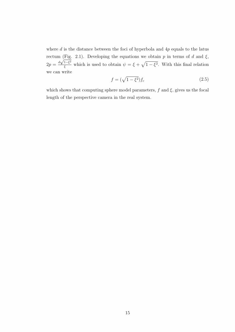
where d is the distance between the foci of hyperbola and 4p equals to the latus

rectum (Fig. 2.1). Developing the equations we obtain p in terms of d and ξ,

2p =d√

1−ξ2ξ

which is used to obtain ψ = ξ +√

1− ξ2. With this final relation

we can write

f = (√

1− ξ2)fc (2.5)

which shows that computing sphere model parameters, f and ξ, gives us the focal

length of the perspective camera in the real system.

15

chapter 3

DLT-Based Calibration of

Sphere Camera Model

In this chapter, we present a calibration technique that is valid for all single-

viewpoint catadioptric cameras. First we review the literature on catadioptric

camera calibration in Section 3.1. Then, based on the introduction given in

Section 2.2 for the sphere camera model, we explain the proposed calibration

technique which estimates the parameters of the sphere camera model. Finally,

in Sections 3.3 and 3.4, we present the results of experiments for the proposed

calibration approach using both simulated and real images.

3.1 Literature on Catadioptric Camera Calibra-

tion

Several methods were proposed for calibration of catadioptric systems. Some

of them consider estimating the parameters of the parabolic [42, 43], hyperbolic

[44] and conical [45] mirrors together with the camera parameters. Calibration of

outgoing rays based on a radial distortion model is another approach. Kannala

and Brandt [46] used this approach to calibrate fisheye cameras. Scaramuzza et

al. [47] extended the approach to include central catadioptric cameras as well.

Mei and Rives [26], on the other hand, developed another Matlab calibration

toolbox that estimates the parameters of the sphere camera model. Parameter

initialization is performed with user input. The user defines the location of the

principal point and depicts a real world straight line in the omnidirectional image

which is used for focal length estimation.

16

Figure 3.1: Block diagram of the proposed calibration technique.

3.2 Proposed Calibration Technique

Recently, Sturm and Barreto [19] showed that employing the sphere camera

model, the catadioptric projection of a 3D point can be modeled using a projection

matrix of size 6 × 10. The calibration method presented here puts this theory

into practice. We compute the generic projection matrix, Pcata, with 3D-2D

correspondences, using a straightforward Direct Linear Transform (DLT) [48]

approach which is based on a set of linear equations. Then, we decompose Pcata to

estimate intrinsic and extrinsic parameters. With these estimates as initial values

of system parameters, we optimize the parameters by minimizing the reprojection

error. The steps of the algorithm are shown in Fig. 3.1. When compared to

the technique of Mei and Rives [26], the only previous work on calibration of

sphere camera model, our approach has the advantages of not requiring input for

parameter initialization and being able to calibrate perspective cameras as well.

On the other hand, our algorithm needs a 3D calibration object.

3.2.1 Mathematical Background on Coordinate Lifting

Lifted coordinates from symmetric matrix equations.

The derivation of (multi-) linear relations for catadioptric imagery requires

the use of lifted coordinates. The Veronese map Vn,d of degree d maps points of

Pn into points of an m dimensional projective space Pm, with m =

(n+ d

d

)−1.

Consider the second order Veronese map V2,2, that embeds the projective plane

into the 5D projective space, by lifting the coordinates of point q to

q =(q2

1 q1q2 q22 q1q3 q2q3 q2

3

)T

17

Vector q and matrix qqT are composed by the same elements. The former

can be derived from the latter through a suitable re-arrangement of parameters.

Define v(U) as the vector obtained by stacking the columns of a generic matrix

U [49]. For the case of qqT, v(qqT) has several repeated elements because of the

matrix symmetry. By left multiplication with a suitable permutation matrix P

that adds the repeated elements, it follows that

q = D−1

( 1 0 0 0 0 0 0 0 00 1 0 1 0 0 0 0 00 0 0 0 1 0 0 0 00 0 1 0 0 0 1 0 00 0 0 0 0 1 0 1 00 0 0 0 0 0 0 0 1

)︸ ︷︷ ︸

P

v(qqT), (3.1)

with D a diagonal matrix, Dii =∑9

j=1 Pij.

If U is symmetric, then it is uniquely represented by vsym(U), the row-wise

vectorization of its lower left triangular part:

vsym(U) = D−1PU = (U11, U21, U22, U31, · · · , Unn)T

Lifted matrices.

Let us now discuss the lifting of linear transformations. Consider a matrix A

to transform a vector q such that r = Aq. The relation rrT = A(qqT)AT can be

written as a vector mapping

(rrT) = (A⊗ A)(qqT),

with ⊗ denoting the Kronecker product [49]. Using the symmetric vectorization,

we have q = vsym(qqT) and r = vsym(rrT), thus:

r = D−1P(A⊗ A)PT︸ ︷︷ ︸A

q (3.2)

where A represents the lifted linear transformation.

Another representation for A is given in the following. Let ai be the columns

of A. Then, employing Eq. 3.1,

A = D−1P(v(a1a

T1 ) 2v(a1a

T2 ) v(a2a

T2 ) 2v(a1a

T3 ) 2v(a2a

T3 ) v(a3a

T3 ))

18

A few useful properties of the lifting of transformations are [49,50]:

AB = AB A−1 = A−1 AT = D−1ATD (3.3)

In our work, we use the following liftings: 3-vectors q to 6-vectors q and 4-

vectors Q to 10-vectors Q. Analogously, 3 × 3 matrices are lifted to 6 × 6 and

3× 4 matrices to 6× 10.

3.2.2 Generic Projection Matrix

As explained in Section 2.2, a 3D point is mathematically projected to two

image points. Sturm and Barreto [19] represented these two 2D points via the

degenerate dual conic generated by them, i.e. the dual conic containing exactly

the lines going through at least one of the two points. Let the two image points

be q+, q−, and the dual conic is given by

Ω ∼ q+qT− + q−qT

+

The vectorized matrix of the conic can be computed as shown below using

the lifted 3D point coordinates, intrinsic and extrinsic parameters.

vsym(Ω) ∼ K6×6XξR6×6

(I6 T6×4

)Q10 (3.4)

Here, R represents the rotation of the catadioptric camera. Xξ and T6×4

depend only on the sphere model parameter ξ and position of the catadioptric

camera C = (tx, ty, tz) respectively, as shown here:

Xξ =

1 0 0 0 0 0

0 1 0 0 0 0

0 0 1 0 0 0

0 0 0 1 0 0

0 0 0 0 1 0

−ξ2 0 −ξ2 0 0 1− ξ2

T6×4 =

−2tx 0 0 t2x

−ty −tx 0 txty

0 −2ty 0 t2y

−tz 0 −tx txtz

0 −tz −ty tytz

0 0 −2tz t2z

Thus, a 6× 10 catadioptric projection matrix, Pcata, can be expressed by

its intrinsic and extrinsic parameters, as in the case of a perspective camera:

19

Pcata = KXξ︸︷︷︸Acata

R6×6

(I6 T6×4

)︸ ︷︷ ︸

Tcata

(3.5)

3.2.3 Computation of the Generic Projection Matrix

Here we show the way used to compose the equations using 3D-2D correspon-

dences to compute Pcata. Analogous to the perspective case ([q]×PQ = 0), we

write the constraint based on the lifted coordinates [19]:

[q]× Pcata Q = 0

where [q]× denotes the skew-symmetric matrix associated with the cross product

of 3-vector q. This is a set of 6 linear homogeneous equations in the coefficients of

Pcata. Using the Kronecker product, this can be written in terms of the 60-vector

pcata containing the 60 coefficients of Pcata:([q]× ⊗ QT

)pcata = 06

Stacking these equations for n 3D-2D correspondences gives an equation sys-

tem of size 6n × 60, which we solve to least squares. Note that the minimum

number of required correspondences is 20: a 3 × 3 skew symmetric matrix has

rank 2, its lifted counterpart rank 3. Therefore, each correspondence provides

only 3 independent linear constraints.

Another observation is that the 3D points should be distributed on at least

three different planes. Here follows a proof of why points on two planes are not

sufficient to compute Pcata using linear equations [51]. Let Π1 and Π2 be the

two planes. Hence, each calibration point Q satisfies(ΠT

1 Q) (

ΠT2 Q)

= 0. This

can be written as a linear constraint on the lifted calibration points: pTQ = 0,

where the 10-vector p depends exactly on the two planes. Thus, if Pcata is the

true 6 × 10 projection matrix, then adding some multiple of pT to any row of

Pcata gives another 6 × 10 projection matrix, Pcata, which maps the calibration

points to the same image entities as the true projection matrix.

Pcata = Pcata + vpT

20

where v is a 6-vector and represents the 6-dof on Pcata that can not be recovered

using only linear projection equations and calibration points located in only two

planes. For three planes, there is no linear equation as above that holds for all

calibration points.

3.2.4 Decomposition of the Generic Projection Matrix

The calibration process consists of getting the intrinsic and extrinsic param-

eters of a camera. Our purpose is to decompose Pcata as in Eq. (3.5). Consider

first the leftmost 6× 6 submatrix of Pcata:

Ps ∼ KXξR

Let us define M = PsD−1PT

s . Using the properties given in Eq. (3.3) and

knowing that for a rotation matrix R−1 = RT, we can write R−1 = D−1RTD.

And from that we obtain D−1 = RD−1RT which we use to eliminate the rotation

parameters:

M ∼ KXξR D−1RTXTξ KT = KXξ D−1XT

ξ KT (3.6)

The above equation holds up to scale, i.e. there is a λ with M = λKXξ D−1XTξ KT.

We use some elements of M to extract the intrinsic parameters:

M16 = λ(−(f 2ξ2) + c2

x(ξ4 + cx(1− ξ2)2

)M44 = λ

(f 2

2+ c2

x(2ξ4 + (1− ξ2)2)

)M46 = λcx(2ξ

4 + (1− ξ2)2)

M56 = λcy(2ξ4 + (1− ξ2)2)

M66 = λ(2ξ4 + (1− ξ2)2

)Note that for the initial computation of intrinsic parameters, we suppose that

there is no tilt in the catadioptric camera, i.e., the perspective camera is not

rotated away from the mirror. We compute the following 4 intrinsic parameters:

ξ, f, cx, cy. The last three are the focal length and principal point coordinates of

the perspective camera in the sphere model. After initialization, the parameters

of tilt and distortion are also estimated by non-linear optimization (Section 3.2.5).

21

Since we obtained M up to a scale, to compute the parameters we should use

ratios between the entries of matrix M. The intrinsic parameters are computed

as follows:

cx =M46

M66

cy =M56

M66

ξ =

√√√√ M16

M66− c2

x

−2(M44

M66− c2

x)

f =

√2(2ξ4 + (1− ξ2)2)

(M44

M66

− c2x

)After extracting the intrinsic part Acata of the projection matrix, we are able

to obtain the 6× 10 extrinsic part Tcata by multiplying Pcata with the inverse of

Acata:

Tcata = R6×6 (I6 T6×4 ) ∼(KXξ

)−1

Pcata (3.7)

So, the leftmost 6× 6 part of Tcata will be the estimate of the lifted rotation

matrix. And if we multiply the inverse of this Rest with the rightmost 6× 4 part

of Tcata, we obtain an estimate for the translation (T6×4). This translation should

have an ideal form as given in Eq. (3.4) and we are able to identify translation

vector elements (tx, ty, tz) from it.

We extract the rotation angles around x, y and z axes one by one using Rest.

First, we recover the rotation angle around the z axis, γ = tan−1(

Rest,51

Rest,41

).

Then, Rest is modified by being multiplied by the inverse of rotation around

z axis, Rest = R−1z,γ Rest. Then, rotation angle around y axis, β, is estimated and

Rest is modified β = tan−1(−Rest,52

Rest,22

), Rest = R−1

y,β Rest

Finally, rotation angle around x axis, α, is estimated by α = tan−1(

Rest,42

Rest,22

).

3.2.5 Other Parameters of Non-linear Calibration

The intrinsic and extrinsic parameters extracted linearly in Section 3.2.4 are

not always adequate to model a real camera. Extra parameters are needed to

correctly model the catadioptric system, namely, tilting and lens distortions.

In Section 2.2.1, we explained why tilt in real catadioptric camera is not

equal to the tilt in the sphere camera model. However, we can still estimate

tilting parameters to remove the effect of such an imperfection. To do this, we

define a rotation, Rp, between camera center and sphere center. Tilting has only

22

Rx and Ry components, because rotation around optical axis, Rz, is merged with

the external rotation around the z axis.

As well known, imperfections due to lenses are modeled as distortions for

camera calibration. Radial distortion models contraction or expansion with re-

spect to the image center and tangential distortion models lateral effects. To add

these distortion effects to our calibration algorithm, we employed the approach

of Heikkila and Silven [52].

Radial distortion is given as

∆x = x(k1r2 + k2r

4 + k3r6 + ..) , ∆y = y(k1r

2 + k2r4 + k3r

6 + ..) (3.8)

where r =√x2 + y2 and k1, k2.. are the radial distortion parameters. We ob-

served that estimating two parameters was sufficient for an adequate modeling.

Tangential distortion is given as

∆x = 2p1xy + p2(r2 + 2x2) , ∆y = p1(r2 + 2y2) + 2p2xy (3.9)

where r =√x2 + y2 and p1, p2 are the tangential distortion parameters.

We applied distortion after projecting the 3D points on the sphere and mod-

ifying the coordinates with ξ (also after applying tilting, if modeled). Thus, in a

sense we distort the rays outgoing from the camera center. Next, distorted rays

are projected to the image by employing camera intrinsic parameters.

Once we have identified all the parameters to be estimated we perform a

non-linear optimization to compute the whole model. We use the Levenberg-

Marquardt (LM) method provided by the function lsqnonlin in Matlab. The

minimization criterion is the root mean square (RMS) of distance error between

a measured image point and its reprojected correspondence. Since the projection

equations we use (cf. Eq. 3.4) map 3D points to dual image conics, we have to

extract the two potential image points from it; the one closer to the measured

point is selected and then the reprojection error is measured. We take as initial

values the parameters obtained from Pcata and initialize the additional distortion

parameters with zero.

23

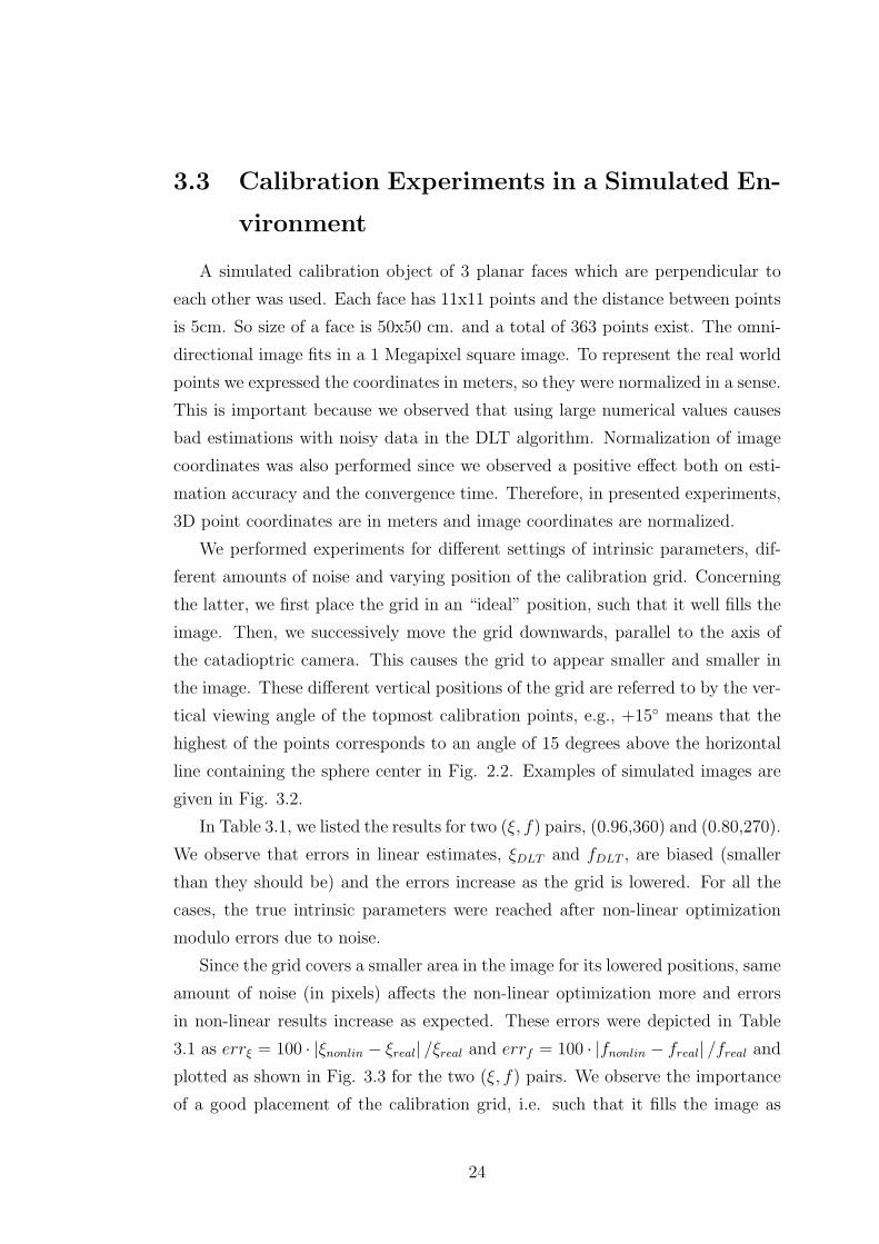
3.3 Calibration Experiments in a Simulated En-

vironment

A simulated calibration object of 3 planar faces which are perpendicular to

each other was used. Each face has 11x11 points and the distance between points

is 5cm. So size of a face is 50x50 cm. and a total of 363 points exist. The omni-

directional image fits in a 1 Megapixel square image. To represent the real world

points we expressed the coordinates in meters, so they were normalized in a sense.

This is important because we observed that using large numerical values causes

bad estimations with noisy data in the DLT algorithm. Normalization of image

coordinates was also performed since we observed a positive effect both on esti-

mation accuracy and the convergence time. Therefore, in presented experiments,

3D point coordinates are in meters and image coordinates are normalized.

We performed experiments for different settings of intrinsic parameters, dif-

ferent amounts of noise and varying position of the calibration grid. Concerning

the latter, we first place the grid in an “ideal” position, such that it well fills the

image. Then, we successively move the grid downwards, parallel to the axis of

the catadioptric camera. This causes the grid to appear smaller and smaller in

the image. These different vertical positions of the grid are referred to by the ver-

tical viewing angle of the topmost calibration points, e.g., +15 means that the

highest of the points corresponds to an angle of 15 degrees above the horizontal

line containing the sphere center in Fig. 2.2. Examples of simulated images are

given in Fig. 3.2.

In Table 3.1, we listed the results for two (ξ, f) pairs, (0.96,360) and (0.80,270).

We observe that errors in linear estimates, ξDLT and fDLT , are biased (smaller

than they should be) and the errors increase as the grid is lowered. For all the

cases, the true intrinsic parameters were reached after non-linear optimization

modulo errors due to noise.

Since the grid covers a smaller area in the image for its lowered positions, same

amount of noise (in pixels) affects the non-linear optimization more and errors

in non-linear results increase as expected. These errors were depicted in Table

3.1 as errξ = 100 · |ξnonlin − ξreal| /ξreal and errf = 100 · |fnonlin − freal| /freal and

plotted as shown in Fig. 3.3 for the two (ξ, f) pairs. We observe the importance

of a good placement of the calibration grid, i.e. such that it fills the image as

24

(a) (b)

(c) (d)

Figure 3.2: Examples of the simulated images with varying values of ξ, f andvertical viewing angle (in degrees) of the highest point in 3D calibration grid (θ).(a) (ξ, f, θ)=(0.96,360,15) (b) (ξ, f, θ)=(0.80,270,15) (c) (ξ, f, θ)=(0.96,360,-15)(d) (ξ, f, θ)=(0.80,270,-15)

much as possible. We also observe that larger ξ and f values produced slightly

better results since errors in Fig. 3.3a are smaller.

3.3.1 Estimation Errors for Different Camera Types

Here we discuss the intrinsic and extrinsic parameter estimation for the two

most common catadioptric systems: hyper-catadioptric and para-catadioptric,

with hyperbolic and parabolic mirror respectively. We also present our observa-

tion for experiments on perspective cameras.

25

Table 3.1: Calibration experiment with simulated images. Initial and optimizedestimates of parameters for varying grid heights and (ξ, f) values.

Vertical viewing angle of the topmost grid points+15 0 −15 −30 −45

ξreal 0.96 0.8 0.96 0.8 0.96 0.8 0.96 0.8 0.96 0.8freal 360 270 360 270 360 270 360 270 360 270ξDLT 0.544 0.405 0.151 0.152 0.084 0.053 0.012 0.043 0.029 0.050fDLT 361 268 296 230 251 198 223 175 211 169ξnonlin 0.960 0.800 0.955 0.793 0.951 0.810 0.991 0.780 0.912 0.750fnonlin 360 270 359 271 362 271 365 266 354 261errξ 0.0 0.0 0.5 0.8 0.9 1.2 3.2 2.5 5.0 6.3errf 0.0 0.1 0.4 0.3 0.6 0.3 1.4 1.3 1.6 3.2

For all columns, cx=cy=500, and α= -0.628, β= 0.628 and γ= 0.175. Amount ofnoise: σ = 1 pixel. ξDLT ,fDLT and ξnonlin,fnonlin are the results of DLT algorithm andnon-linear optimization respectively, errξ and errf are the relative errors, in percent.

Hyper-catadioptric system.

Table 3.2 shows non-linear optimization experiment results for two different

noise levels (σ = 0.5, σ = 1), when the described 3D pattern is used and maximum

vertical angle of pattern points is +15.

Para-catadioptric system.

Parabolic mirror has a ξ = 1, which has a potential to destabilize the esti-

mations because Xξ becomes a singular matrix. We observed that the results

of DLT algorithm were not close to the actual values when compared to hyper-

catadioptric system (initial values in Table 3.2). However, non-linear optimiza-

tion was able to estimate the parameters as successful as the hyper-catadioptric

examples given in Table 3.2.

Perspective camera.

In sphere camera model, ξ = 0 corresponds to the perspective camera. Our es-

timation in linear and non-linear steps are as successful as the hyper-catadioptric

case.

26

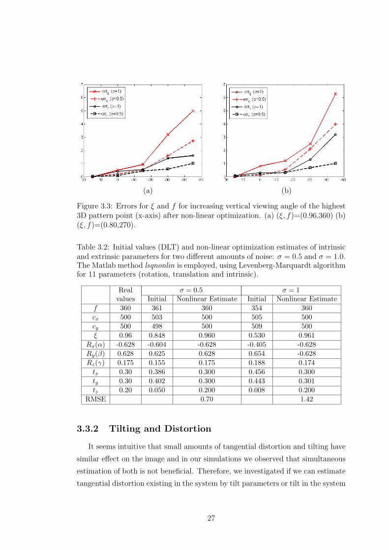
(a) (b)

Figure 3.3: Errors for ξ and f for increasing vertical viewing angle of the highest3D pattern point (x-axis) after non-linear optimization. (a) (ξ, f)=(0.96,360) (b)(ξ, f)=(0.80,270).

Table 3.2: Initial values (DLT) and non-linear optimization estimates of intrinsicand extrinsic parameters for two different amounts of noise: σ = 0.5 and σ = 1.0.The Matlab method lsqnonlin is employed, using Levenberg-Marquardt algorithmfor 11 parameters (rotation, translation and intrinsic).

Real σ = 0.5 σ = 1values Initial Nonlinear Estimate Initial Nonlinear Estimate

f 360 361 360 354 360cx 500 503 500 505 500cy 500 498 500 509 500ξ 0.96 0.848 0.960 0.530 0.961

Rx(α) -0.628 -0.604 -0.628 -0.405 -0.628Ry(β) 0.628 0.625 0.628 0.654 -0.628Rz(γ) 0.175 0.155 0.175 0.188 0.174tx 0.30 0.386 0.300 0.456 0.300ty 0.30 0.402 0.300 0.443 0.301tz 0.20 0.050 0.200 0.008 0.200

RMSE 0.70 1.42

3.3.2 Tilting and Distortion

It seems intuitive that small amounts of tangential distortion and tilting have

similar effect on the image and in our simulations we observed that simultaneous

estimation of both is not beneficial. Therefore, we investigated if we can estimate

tangential distortion existing in the system by tilt parameters or tilt in the system

27

Table 3.3: Estimating tangential distortion with tilt parameters. σ = 0.5 pixels.

Real p1 = p2 = 0.006 p1 = p2 = −0.003values Initial Nonlin. Estimate Initial Nonlin. Estimate

f 180 196.5 179.4 195.6 180.3cx 500 508.2 495.6 507.0 501.9cy 500 486.9 495.9 485.7 502.5ξ 0.96 1.037 0.9579 1.041 0.9617

tiltx 0 -0.0349 0 0.0187tilty 0 0.0367 0 -0.0171k1 -0.06 0 -0.061 0 -0.059k2 0.006 0 0.006 0 0.0058

RMSE 0.85 0.7

by tangential distortion parameters.

When there is no tilt but only tangential distortion and we estimate tilting

parameters, we observed that the direction and amount of tiltx, tilty, cx and cy

changes proportional to the tangential distortion applied and RMSE decreases.

Table 3.3 shows the results for this experiment. We observe that having a tangen-

tial distortion of p1 = 0.006 results in ∼ 0.036 change in tiltx and ∼ 4.5 pixels

change in cx.

However, RMSE does not reach the values when there is no distortion. In

noiseless case, for example, final RMSe are 0.48 for p1 = p2 = 0.006 and 0.27 for

p1 = p2 = −0.003.

Hence, we conclude that tilt parameters compensate the tangential distortion

effect up to an extent, but not perfectly. We also investigated if tilting can be

compensated by tangential distortion parameters and we had very similar results.

Thus, tangential distortion parameters have the same capability to estimate tilt-

ing. Also knowing from Section 2.2.1 that the tilt in the sphere camera model

is not equivalent to the tilt in real catadioptric camera, we decided to continue

with estimating tangential distortion parameters.

28

(a) (b)

Figure 3.4: (a) Omnidirectional image of the 3D pattern (1280×960 pixels, flippedhorizontal). (b) Constructed model of the 3D pattern.

3.4 Calibration with Real Images using a 3D

Pattern

In this section, we perform calibration using a 3D pattern. We use an omni-

directional image viewing the 3D pattern (Fig. 3.4a) and we construct the 3D

model of the pattern knowing the distances between the corners of the pattern

(Fig. 3.4b). A one megapixel omnidirectional image was acquired using a cata-

dioptric system comprising a 1/2 inch CCD camera (Imaging Source DFK 41F02)

and a omnidirectional viewing apparatus with a parabolic mirror (Remote Reality

S80).

We computed, from a total of 144 3D-2D correspondences, the projection

matrix Pcata and extracted the intrinsic and extrinsic parameters as explained in

Section 3.2. From the simulations, we observed that we have better estimations

if the 3D-2D correspondences are in the same order of magnitude. Therefore,

3D points are given in meters and 2D points are normalized so that the centroid

of the reference points is at the origin of coordinates and mean distance of the

points from the origin is equal to√

2.

The experiment is focused on obtaining the intrinsic parameters from Pcata

with DLT approach to get initial estimates of these values and optimizing these

parameters together with distortion parameters with a non-linear optimization

step based on the reprojection error. Table 3.4 shows the estimation results and

29

Table 3.4: Intrinsic parameters estimated with the proposed calibration approach.

parameters Initial estimates Final estimates Final estimates (ξ=1 restricted)f 314.7 550.3 435.0cx 563.0 543.1 542.4cy 347.5 511.0 509.5ξ 0.339 1.475 1.0k1 0 0.180 -0.060k2 0 0.235 0.008t1 0 0.024 0.006t2 0 -0.006 -0.003

RMSE 134.0 0.368 0.395

(a) (b)

Figure 3.5: Reprojections with the estimated parameters after initial (DLT) step(a) and after non-linear optimization step (b).

in Fig. 3.5 one can see the reprojections with the estimated parameters for initial

values (a) and values after nonlinear estimation (b).

We observe from the third column of Table 3.4 that, when unrestricted, final

ξ estimate is much larger than its theoretical value of 1.0. Focal length (f) and

radial distortion parameters (k1,k2) compensate this high ξ value resulting in a

low reprojection error seen in Fig. 3.5b. Alternatively, we can apply a restriction

such as ξ = 1.0 in optimization step. In this case we obtain the results given in

the last column of Table 3.4. Although the reprojection error is not lower than

30

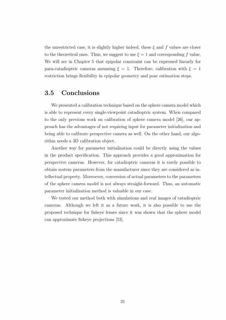
the unrestricted case, it is slightly higher indeed, these ξ and f values are closer

to the theoretical ones. Thus, we suggest to use ξ = 1 and corresponding f value.

We will see in Chapter 5 that epipolar constraint can be expressed linearly for

para-catadioptric cameras assuming ξ = 1. Therefore, calibration with ξ = 1

restriction brings flexibility in epipolar geometry and pose estimation steps.

3.5 Conclusions

We presented a calibration technique based on the sphere camera model which

is able to represent every single-viewpoint catadioptric system. When compared

to the only previous work on calibration of sphere camera model [26], our ap-

proach has the advantages of not requiring input for parameter initialization and

being able to calibrate perspective camera as well. On the other hand, our algo-

rithm needs a 3D calibration object.

Another way for parameter initialization could be directly using the values

in the product specification. This approach provides a good approximation for

perspective cameras. However, for catadioptric cameras it is rarely possible to

obtain system parameters from the manufacturer since they are considered as in-

tellectual property. Moreoever, conversion of actual parameters to the parameters

of the sphere camera model is not always straight-forward. Thus, an automatic

parameter initialization method is valuable in our case.

We tested our method both with simulations and real images of catadioptric

cameras. Although we left it as a future work, it is also possible to use the

proposed technique for fisheye lenses since it was shown that the sphere model

can approximate fisheye projections [53].

31

chapter 4

Feature Matching

In this chapter, we present our method of matching feature points between

mixed camera images. In Section 4.1, we describe the proposed algorithm to

increase the matching performance of Scale Invariant Feature Transform (SIFT)

and to eliminate the false matches in the SIFT output. In Section 4.2, we briefly

decribe how to create virtual camera plane (VCP) images for matching. Finally,

in Section 4.3 we present the results of experiments conducted with catadioptric

and fish-eye cameras, showing that matching performance significantly increases

with the proposed approaches.

4.1 Improving the Initial SIFT Output

To match features in hybrid image pairs automatically, we employ SIFT and

propose an algorithm to obtain better feature matches between catadioptric and

perspective images.

SIFT detects features in the so-called scale space comprising levels and octaves

which are obtained by low-pass filtering and downsampling the original image sys-

tematically [21]. This enables the detection of features at different scales. In our

case of matching points between images of different resolutions, a feature in the

perspective image can be matched to a feature in the catadioptric image. How-

ever, we observed that, together with the correct matches, a considerable number

of false matches occur in the SIFT output due to matching a high-resolution

feature in perspective image to a feature in catadioptric image which is lower

resolution.

Table 4.1 shows the number of extracted features in different octaves for im-

ages Pers2 and Omni2 (Fig. 4.7). There is an approximate ratio between scales

of true correspondences (SR=σpers/σomni), which is ≈3.6 for the given images.

Corresponding octaves of correct matches are indicated in the table with arrows.

32

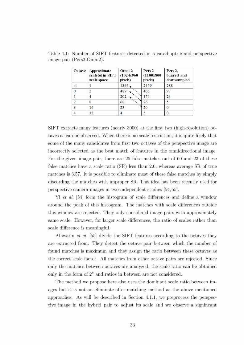
Table 4.1: Number of SIFT features detected in a catadioptric and perspectiveimage pair (Pers2-Omni2).

SIFT extracts many features (nearly 3000) at the first two (high-resolution) oc-

taves as can be observed. When there is no scale restriction, it is quite likely that

some of the many candidates from first two octaves of the perspective image are

incorrectly selected as the best match of features in the omnidirectional image.

For the given image pair, there are 25 false matches out of 60 and 23 of these

false matches have a scale ratio (SR) less than 2.0, whereas average SR of true

matches is 3.57. It is possible to eliminate most of these false matches by simply

discarding the matches with improper SR. This idea has been recently used for

perspective camera images in two independent studies [54,55].

Yi et al. [54] form the histogram of scale differences and define a window

around the peak of this histogram. The matches with scale differences outside

this window are rejected. They only considered image pairs with approximately

same scale. However, for larger scale differences, the ratio of scales rather than

scale difference is meaningful.

Alhwarin et al. [55] divide the SIFT features according to the octaves they

are extracted from. They detect the octave pair between which the number of

found matches is maximum and they assign the ratio between these octaves as

the correct scale factor. All matches from other octave pairs are rejected. Since

only the matches between octaves are analyzed, the scale ratio can be obtained

only in the form of 2k and ratios in between are not considered.

The method we propose here also uses the dominant scale ratio between im-

ages but it is not an eliminate-after-matching method as the above mentioned

approaches. As will be described in Section 4.1.1, we preprocess the perspec-

tive image in the hybrid pair to adjust its scale and we observe a significant

33

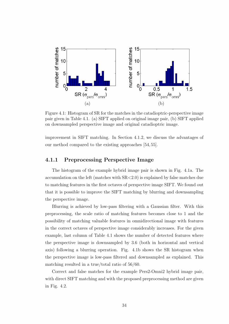
(a) (b)

Figure 4.1: Histogram of SR for the matches in the catadioptric-perspective imagepair given in Table 4.1. (a) SIFT applied on original image pair, (b) SIFT appliedon downsampled perspective image and original catadioptric image.

improvement in SIFT matching. In Section 4.1.2, we discuss the advantages of

our method compared to the existing approaches [54,55].

4.1.1 Preprocessing Perspective Image

The histogram of the example hybrid image pair is shown in Fig. 4.1a. The

accumulation on the left (matches with SR<2.0) is explained by false matches due

to matching features in the first octaves of perspective image SIFT. We found out

that it is possible to improve the SIFT matching by blurring and downsampling

the perspective image.

Blurring is achieved by low-pass filtering with a Gaussian filter. With this

preprocessing, the scale ratio of matching features becomes close to 1 and the

possibility of matching valuable features in omnidirectional image with features

in the correct octaves of perspective image considerably increases. For the given

example, last column of Table 4.1 shows the number of detected features where

the perspective image is downsampled by 3.6 (both in horizontal and vertical

axis) following a blurring operation. Fig. 4.1b shows the SR histogram when

the perspective image is low-pass filtered and downsampled as explained. This

matching resulted in a true/total ratio of 56/60.

Correct and false matches for the example Pers2-Omni2 hybrid image pair,

with direct SIFT matching and with the proposed preprocessing method are given

in Fig. 4.2.

34

Figure 4.2: Matching results for the Pers2-Omni2 image pair with direct matchingresulted in 25/60 false/total match ratio (at the top) and with the proposedpreprocessing method resulted in 4/60 false/total match ratio (at the bottom).Red dashed lines indicate false matches, whereas green lines indicate correct ones.

The parameters of downsampling and low-pass filtering. We selected

the downsampling factor from the histogram as the mean of the most dominant

Gaussian in the mixture, because the SIFT scale space ratio also reveals the scale

ratio of features in the images. To avoid aliasing, we need to low-pass filter the

perspective image before downsampling. We selected the cut-off frequency as

2.5/σ in the frequency domain and the standard deviation of the Gaussian filter

for the blurring becomes σ = 2.5d/π where d is the downsampling factor. Figure

4.3 shows the discrete time FFT graphs before and after the described low-pass

35

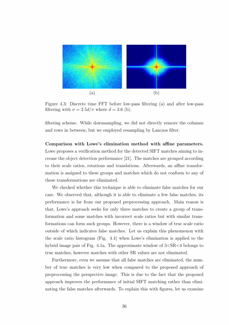
(a) (b)

Figure 4.3: Discrete time FFT before low-pass filtering (a) and after low-passfiltering with σ = 2.5d/π where d = 3.6 (b).

filtering scheme. While downsampling, we did not directly remove the columns

and rows in between, but we employed resampling by Lanczos filter.

Comparison with Lowe’s elimination method with affine parameters.

Lowe proposes a verification method for the detected SIFT matches aiming to in-

crease the object detection performance [21]. The matches are grouped according

to their scale ratios, rotations and translations. Afterwards, an affine transfor-

mation is assigned to these groups and matches which do not conform to any of

these transformations are eliminated.

We checked whether this technique is able to eliminate false matches for our

case. We observed that, although it is able to eliminate a few false matches, its

performance is far from our proposed preprocessing approach. Main reason is

that, Lowe’s approach seeks for only three matches to create a group of trans-

formation and some matches with incorrect scale ratios but with similar trans-

formations can form such groups. However, there is a window of true scale ratio

outside of which indicates false matches. Let us explain this phenomenon with

the scale ratio histogram (Fig. 4.4) when Lowe’s elimination is applied to the

hybrid image pair of Fig. 4.1a. The approximate window of 3<SR<4 belongs to

true matches, however matches with other SR values are not eliminated.

Furthermore, even we assume that all false matches are eliminated, the num-

ber of true matches is very low when compared to the proposed approach of

preprocessing the perspective image. This is due to the fact that the proposed

approach improves the performance of initial SIFT matching rather than elimi-

nating the false matches afterwards. To explain this with figures, let us examine

36

Figure 4.4: Histogram of SR for the matches of the catadioptric-perspective imagepair given in Table 4.1 when Lowe’s elimination is applied.

the entries in Table 4.2 for the same example hybrid image pair (Pers2-Omni2).

The table also shows the results of VCP approach (Section 4.2). True/False ratios

for Pers2-Omni2 and Pers2-VCP2 pairs are not satisfactory even with the elimi-

nation proposed by Lowe, however when the perspective image is preprocessed as

proposed (bold-face lines), results are significantly improved. Therefore, prepro-

cessing the perspective image increases the performance of SIFT matching with

or without employing the elimination with affine parameters.

We also observe that, the results are slightly better with Lowe’s elimination.

Thus, elimination with the assumption of an affine transformation works up to

an extent although it is not a good approximation especially when we work on

hybrid pairs. Moreover, the elimination of matches that do not conform to a

transformation is not crucial at this step since we do eliminate the matches that

do not conform to the epipolar geometry during the estimation of fundamental

matrix with RANSAC (cf. Chapter 5) which imposes a more accurate geometrical

constraint.

Sensitivity to varying preprocessing parameters. So far, we described

the procedure of preprocessing the perspective image and selection of low-pass

filtering and downsampling parameters. Fig. 4.5 shows the number of correct

matches for varying low-pass filering (σ) and downsampling (d) parameters for

the example mixed image pair. We observe that the performance with the selected

parameters is quite close to the peak and all the parameter pairs represented in

37

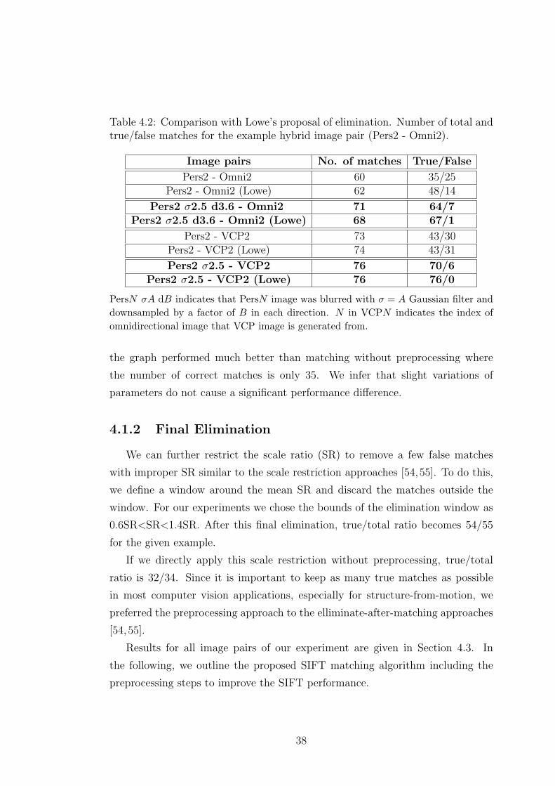
Table 4.2: Comparison with Lowe’s proposal of elimination. Number of total andtrue/false matches for the example hybrid image pair (Pers2 - Omni2).

Image pairs No. of matches True/False

Pers2 - Omni2 60 35/25Pers2 - Omni2 (Lowe) 62 48/14

Pers2 σ2.5 d3.6 - Omni2 71 64/7Pers2 σ2.5 d3.6 - Omni2 (Lowe) 68 67/1

Pers2 - VCP2 73 43/30Pers2 - VCP2 (Lowe) 74 43/31

Pers2 σ2.5 - VCP2 76 70/6Pers2 σ2.5 - VCP2 (Lowe) 76 76/0

PersN σA dB indicates that PersN image was blurred with σ = A Gaussian filter anddownsampled by a factor of B in each direction. N in VCPN indicates the index ofomnidirectional image that VCP image is generated from.

the graph performed much better than matching without preprocessing where

the number of correct matches is only 35. We infer that slight variations of

parameters do not cause a significant performance difference.

4.1.2 Final Elimination

We can further restrict the scale ratio (SR) to remove a few false matches

with improper SR similar to the scale restriction approaches [54,55]. To do this,

we define a window around the mean SR and discard the matches outside the

window. For our experiments we chose the bounds of the elimination window as

0.6SR<SR<1.4SR. After this final elimination, true/total ratio becomes 54/55

for the given example.

If we directly apply this scale restriction without preprocessing, true/total

ratio is 32/34. Since it is important to keep as many true matches as possible

in most computer vision applications, especially for structure-from-motion, we

preferred the preprocessing approach to the elliminate-after-matching approaches

[54,55].

Results for all image pairs of our experiment are given in Section 4.3. In

the following, we outline the proposed SIFT matching algorithm including the

preprocessing steps to improve the SIFT performance.

38

Figure 4.5: Number of correct matches out of 60 matches for varying low-passfiltering (σ) and downsampling (d) parameters for the example mixed image pair(Table 4.1).

Algorithm 4.1: Hybrid SIFT matching with the proposed approach

1. Extract downsampling factor. Apply SIFT matching between the given

perspective and catadioptric image pair and plot the histogram of scale ra-

tios (eg. Fig. 4.1a). Select the downsampling factor (d) from the histogram

as the mean of the most dominant Gaussian in the mixture.

2. Preprocess the perspective image. Low-pass filter the perspective im-

age with a Gaussian filter having a σ = 2.5d/π and downsample the low-pass

filtered image by d both in horizontal and vertical directions.

3. Perform SIFT. Apply SIFT matching between the preprocessed perspec-

tive image and catadioptric image.

4. Perform final elimination. Plot the histogram of scale ratios (SR)

for the final matching (eg. Fig. 4.1b) and select only the matches with

0.6SR<SR<1.4SR.

39

4.2 Creating Virtual Camera Plane Images

Another approach that can be employed in conjuction with preprocessing

method is to use so-called virtual camera planes (VCP) to create virtual perspec-

tive images from omnidirectional images and perform matching between VCP and

perspective images. If the omnidirectional camera is calibrated, i.e. if the intrin-

sic parameters of the camera are known, catadioptric-to-VCP or fisheye-to-VCP

conversion can easily be performed.

To generate virtual perspective image, a virtual camera plane with a certain

viewing direction (azimuth), a vertical angle and a distance from the mirror focal

point (origin) have to be defined (Fig. 4.6). To find the intensity value of a pixel

in the virtual perspective image (xv, yv), corresponding pixel coordinates in the

paraboloidal catadioptric image (xi, yi) are given by [56]:

xi = h

ZS+√d2XS yi = h

ZS+√d2YS (4.1)

where, d =√XS

2 + YS2 + ZS

2 and (XS, YS, ZS) are the 3D coordinates of the

virtual image pixel w.r.t. the origin. These coordinates are computed using the

assigned azimuth, vertical angle and distance value for the virtual plane.

If the calibration information is not available for a para-catadioptric image,

we can recover the mirror parameter h by assigning a position in the image which

corresponds to an object with the same height with mirror focal point. The

distance between the image center and that point gives us the parameter h in

terms of pixels, for example the radius of white circle in the top-left image of Fig.

4.8. The principal point can be assumed to be at the center of omnidirectional

image circle.

VCP image can be created using the sphere model parameters in the same

manner. A VCP with an azimuth, a vertical angle and a distance from the

viewpoint (center of sphere) is defined and for each pixel in the VCP, its 3D ray

and corresponding pixel coordinates in the catadioptric image are determined

with sphere model parameters.

Created virtual images are matched with the perspective camera images view-

ing the same scene. When we create VCP images with sizes close to the size of

perspective images, SR of the true matches is close to 1.0 and no downsampling

40

Figure 4.6: Generation of a virtual perspective image in a paraboloidal omnidi-rectional camera.

is needed. However, since the VCP image is created by interpolating the limited

number of pixels in the omnidirectional image the resolution difference still ex-

ist between perspective and VCP image. Therefore, we again low-pass filter the

perspective image to balance its resolution, i.e. we perform the second step of

Algorithm 4.1 (Section 4.1.2, p.39) without the downsampling part. Alternatively

we could have produced a small-size VCP and downsampled the perspective im-

age after low-pass filtering. In our experiments, we observed that it produces

similar results. The results of our experiments are given in Section 4.3.

4.3 Experiments

4.3.1 Experiments with Catadioptric Cameras

We conducted tests using two types of catadioptric apparatus, namely Remote

Reality S80 Optic1 and 0-360 Panoramic Optic2 and captured images in indoor

and outdoor environments, respectively.

1http://www.remotereality.com2http://www.0-360.com

41

To detect and match feature points, we used SIFT implementation of Andrea

Vedaldi3 with a modification to provide one-to-one matching. In the original

algorithm it is possible for many points in the first image to match to the same

point in the second image. This causes inconsistencies depending on which image

is defined as “first”. To eliminate this problem, we run the SIFT algorithm in

both ways changing the order of images and declare a match only if it is found

in both runs.

As the output of the catadioptric system is viewed through a mirror, the

objects are flipped in the image. This is corrected by flipping the image w.r.t. a

line passing through the center of catadioptric image circle.

For different hybrid camera pairs and varying baseline length, performances of

direct perspective-omnidirectional matching, preprocessed perspective-omnidirec-

tional matching and preprocessed perspective-VCP matching approaches are com-

pared. To keep the number of matched points same for different trials of an image

pair, we adjusted the matching threshold of SIFT, which defines the strength of

the matched point w.r.t. the second candidate match. Let D1 and D2 be the SIFT

descriptor vectors of two points in the first and second image respectively and t

is the matching threshold. D1 is matched to D2 only if the distance d(D1,D2)

multiplied by t is not greater than the distance of D1 to all other descriptors in

the second image. Typically t is chosen as 1.5.

Indoor Experiment. The images of this first experiment were captured with

the Remote Reality S80 Optic in a controlled indoor environment. The locations

and orientations of the cameras and objects in our scene are given in Fig. 4.7 and

corresponding images are given in Fig. 4.8. Omnidirectional images have a size

of 1024x960 pixels, whereas perspective and VCP images are 1100x800 pixels.

With this setup, we are able to investigate the effect of increasing baseline both

in the direction towards the scene and perpendicular to the scene.

Matching results are shown in Table 4.3. As described in Section 4.1, to

increase the performance, we downsampled the perspective images after low-pass

filtering with a Gaussian filter. In Table 4.3, PersN σA dB indicates that PersN

image was low-pass filtered with σ = A Gaussian filter and downsampled by a

factor of B in each direction. The extraction of these parameters are explained

3http://vision.ucla.edu/∼vedaldi/code/sift/sift.html

42

Figure 4.7: Locations and orientations of cameras in the indoor environmentcatadioptric-perspective point matching experiment.

in Section 4.1.1. Results of matching with VCP approach are also given in Table

4.3. N in VCPN indicates the index of omnidirectional image from which it

is generated. As explained in Section 4.2 we match the VCP images with the

low-pass filtered perspective images.

We plot the ratio of true/total matches in Fig. 4.9 for different approaches.

The table also shows, in the last column, the final true/false ratios obtained after

applying final scale ratio elimination. We do not plot these ratios because the

number of true matches is also important along with the ratio (cf. Section 4.1.2).

Please note that the success rates of both downsampling and VCP approaches in

Fig. 4.9 (solid lines) are further increased by this final elimination.

Pers1, Pers2 and Pers3 have approximately 30cm., 60 cm. and 90 cm. lat-

eral baselines with omnidirectional cameras respectively. We observe that the

matching performance decreases with increasing baseline for all approaches and

the number of false matches decreases significantly for both downsampling and

VCP approaches. VCP approach is more robust to increase in baseline at least

for PersN -Omni1 pairs. We also observe that ratios of PersN -Omni1 pairs are

higher. Since the scene is represented with a larger area in Omni1, this resulted

in an increased number of correct matches.

Outdoor Experiment. The images of this second experiment were captured

with the 0-360 Panoramic Optic and shown in Fig. 4.11. The locations and

43

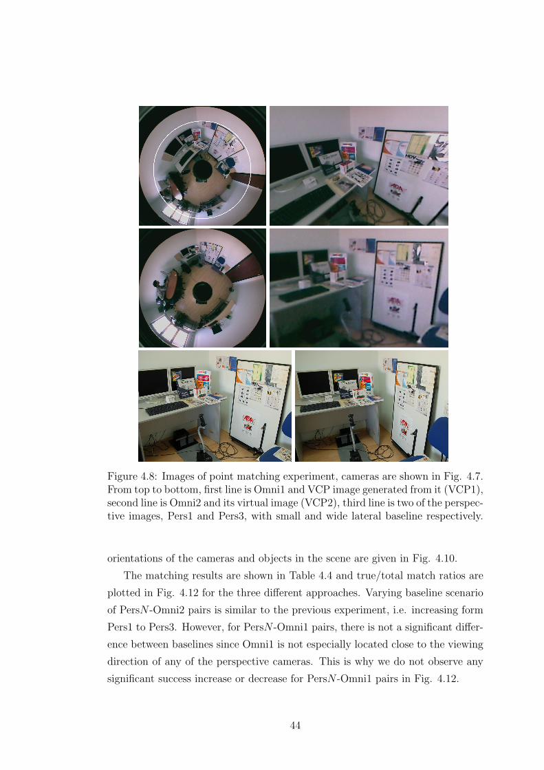
Figure 4.8: Images of point matching experiment, cameras are shown in Fig. 4.7.From top to bottom, first line is Omni1 and VCP image generated from it (VCP1),second line is Omni2 and its virtual image (VCP2), third line is two of the perspec-tive images, Pers1 and Pers3, with small and wide lateral baseline respectively.

orientations of the cameras and objects in the scene are given in Fig. 4.10.

The matching results are shown in Table 4.4 and true/total match ratios are

plotted in Fig. 4.12 for the three different approaches. Varying baseline scenario

of PersN -Omni2 pairs is similar to the previous experiment, i.e. increasing form

Pers1 to Pers3. However, for PersN -Omni1 pairs, there is not a significant differ-

ence between baselines since Omni1 is not especially located close to the viewing

direction of any of the perspective cameras. This is why we do not observe any

significant success increase or decrease for PersN -Omni1 pairs in Fig. 4.12.

44

Table 4.3: Matching results for the image pairs of indoor matching experiment.True/false match ratios (T/F) after the initial and scale restricted matching.

Image pairs no. of T/F T/Fmatches (T/total %) final

Pers1 - Omni1 100 97/3 (97%) 84/1Pers1 σ1.5 d1.65 - Omni1 100 99/1 (99%) 94/0

Pers1 σ1.5 - VCP1 100 99/1 (99%) 99/0Pers2 - Omni1 75 56/19 (75%) 51/7

Pers2 σ1.5 d1.65 - Omni1 75 70/5 (93%) 67/3Pers2 σ1.5 - VCP1 75 73/2 (97%) 73/1

Pers3 - Omni1 60 42/18 (70%) 39/9Pers3 σ1.5 d1.65 - Omni1 60 50/10 (83%) 50/6

Pers3 σ1.5 - VCP1 60 57/3 (95%) 57/1Pers1 - Omni2 80 63/17 (79%) 62/1

Pers1 σ2.5 d3.6 - Omni2 80 80/0 (100%) 80/0Pers1 σ2.5 - VCP2 80 80/0 (100%) 80/0

Pers2 - Omni2 60 35/25 (58%) 32/2Pers2 σ2.5 d3.6 - Omni2 60 56/4 (93%) 54/1

Pers2 σ2.5 - VCP2 60 56/4 (93%) 56/3Pers3 - Omni2 45 15/30 (33%) 15/1

Pers3 σ2.5 d3.3 - Omni2 45 35/10 (78%) 30/8Pers3 σ2.5 - VCP2 45 37/8 (82%) 35/3

PersN σA dB indicates that PersN image was low-pass filtered with σ = A Gaussianfilter and downsampled by a factor of B in each direction.

Figure 4.9: The true/total match ratios (in percentage) for Omni1-PersN (on theleft) and Omni2-PersN (on the right).

45

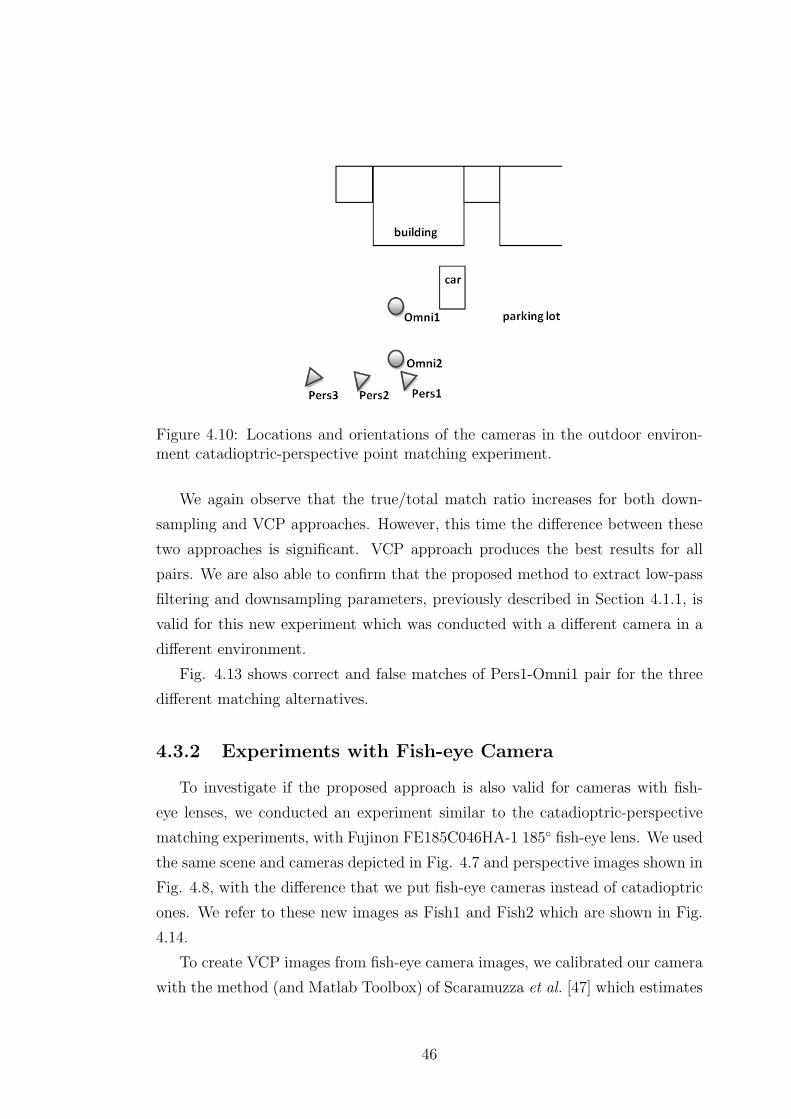
Figure 4.10: Locations and orientations of the cameras in the outdoor environ-ment catadioptric-perspective point matching experiment.

We again observe that the true/total match ratio increases for both down-

sampling and VCP approaches. However, this time the difference between these

two approaches is significant. VCP approach produces the best results for all

pairs. We are also able to confirm that the proposed method to extract low-pass

filtering and downsampling parameters, previously described in Section 4.1.1, is

valid for this new experiment which was conducted with a different camera in a

different environment.

Fig. 4.13 shows correct and false matches of Pers1-Omni1 pair for the three

different matching alternatives.

4.3.2 Experiments with Fish-eye Camera

To investigate if the proposed approach is also valid for cameras with fish-

eye lenses, we conducted an experiment similar to the catadioptric-perspective

matching experiments, with Fujinon FE185C046HA-1 185 fish-eye lens. We used

the same scene and cameras depicted in Fig. 4.7 and perspective images shown in

Fig. 4.8, with the difference that we put fish-eye cameras instead of catadioptric

ones. We refer to these new images as Fish1 and Fish2 which are shown in Fig.

4.14.

To create VCP images from fish-eye camera images, we calibrated our camera

with the method (and Matlab Toolbox) of Scaramuzza et al. [47] which estimates

46

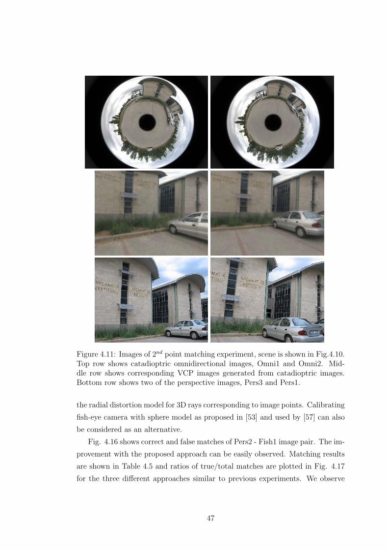
Figure 4.11: Images of 2nd point matching experiment, scene is shown in Fig.4.10.Top row shows catadioptric omnidirectional images, Omni1 and Omni2. Mid-dle row shows corresponding VCP images generated from catadioptric images.Bottom row shows two of the perspective images, Pers3 and Pers1.

the radial distortion model for 3D rays corresponding to image points. Calibrating

fish-eye camera with sphere model as proposed in [53] and used by [57] can also

be considered as an alternative.

Fig. 4.16 shows correct and false matches of Pers2 - Fish1 image pair. The im-

provement with the proposed approach can be easily observed. Matching results

are shown in Table 4.5 and ratios of true/total matches are plotted in Fig. 4.17

for the three different approaches similar to previous experiments. We observe

47

Table 4.4: Matching results for the image pairs of outdoor matching experiment.True/false match ratios (T/F) after the initial and scale restricted matching.

Image pairs no. of T/F T/Fmatches (T/total %) final

Pers1 - Omni1 60 28/32 (47%) 26/6Pers1 σ3.0 d3.5 - Omni1 60 44/16 (73%) 40/10

Pers1 σ3.0 - VCP1 60 57/3 (95%) 53/2Pers2 - Omni1 60 30/30 (50%) 27/5

Pers2 σ2.5 d3.0 - Omni1 60 45/15 (75%) 41/7Pers2 σ2.5 - VCP1 60 56/4 (93%) 51/2

Pers3 - Omni1 60 31/29 (52%) 23/9Pers3 σ2.5 d3.0 - Omni1 60 40/20 (67%) 36/14

Pers3 σ2.5 - VCP1 60 57/3 (95%) 55/2Pers1 - Omni2 75 47/28 (63%) 47/1

Pers1 σ3.5 d4.8 - Omni2 75 64/11 (85%) 61/5Pers1 σ3.5 - VCP2 75 75/0 (100%) 73/0

Pers2 - Omni2 60 33/27 (55%) 32/3Pers2 σ3.0 d4.2 - Omni2 60 49/11 (82%) 46/9

Pers2 σ3.0 - VCP2 60 60/0 (100%) 59/0Pers3 - Omni2 60 29/31 (48%) 27/4

Pers3 σ2.5 d3.3 - Omni2 60 34/26 (57%) 30/19Pers3 σ2.5 - VCP2 60 54/6 (90%) 52/4

PersN σA dB indicates that PersN image was low-pass filtered with σ = A Gaussianfilter and downsampled by a factor of B in each direction.

Figure 4.12: The true/total match ratios (in percentage) of outdoor environmentcatadioptric-perspective point matching experiment (cf. Fig. 4.11 and Fig. 4.10).

48

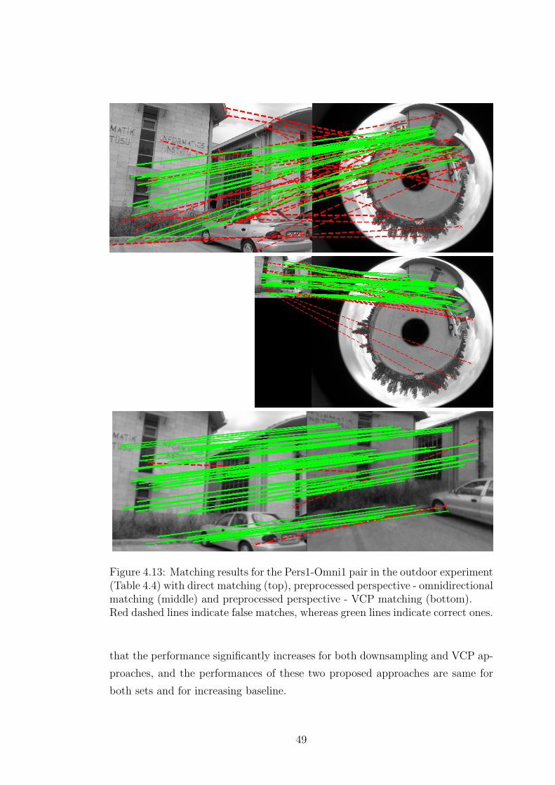
Figure 4.13: Matching results for the Pers1-Omni1 pair in the outdoor experiment(Table 4.4) with direct matching (top), preprocessed perspective - omnidirectionalmatching (middle) and preprocessed perspective - VCP matching (bottom).Red dashed lines indicate false matches, whereas green lines indicate correct ones.

that the performance significantly increases for both downsampling and VCP ap-

proaches, and the performances of these two proposed approaches are same for

both sets and for increasing baseline.

49

Figure 4.14: Fish-eye camera images of the point matching experiment: Fish1(left) and Fish2 (right). The scene is given in Fig. 4.10. Fish1 and Fish2 are atthe same location with Omni1 and Omni2, respectively.

Figure 4.15: A perspective fish-eye hybrid image pair, where the common featuresare not located at the central part of the fish-eye image but closer to periphery.

When compared to the results of experiments with catadioptric cameras, we

are able to say that performance of VCP approach did not change for fish-eye

images, however performance of low-pass filtering and downsampling approach

increased. A possible reason is that the scene represented in fish-eye cameras is

closer to the perspective images when compared to catadioptric cameras (please

compare Fig. 4.14 with Figures 4.8 and 4.11). We also investigated if this result

is valid when the features are not located at the central part of the fish-eye image

but closer to periphery, such as the hybrid image pair given in Fig. 4.15. We

again observed that downsampling approach is as successful as VCP approach.

50

Figure 4.16: Matching results for the Pers2-Fish1 pair in the fish-eye experiment(Table 4.5) with direct matching (top) and downsampling approaches (bottom).Red dashed lines indicate false matches, whereas green lines indicate correct ones.

Figure 4.17: The true/total match ratios (in percentage) of fisheye-perspectivepoint matching experiment (cf. Figs. 4.7 and 4.14).

51

Table 4.5: Matching results for the fisheye-perspective matching experiment.True/false match ratios (T/F) after the initial and scale restricted matching.

Image pairs no. of T/F T/Fmatches (T/total %) final

Pers1 - Fish1 100 84/16 (84%) 82/5Pers1 σ1.5 d1.43 - Fish1 100 99/1 (99%) 98/1

Pers1 σ1.5 - VCP1 100 99/1 (99%) 98/1Pers2 - Fish1 75 54/21 (72%) 53/4

Pers2 σ1.5 d1.43 - Fish1 75 74/1 (99%) 74/1Pers2 σ1.5 - VCP1 75 74/1 (99%) 74/1

Pers3 - Fish1 50 26/24 (52%) 25/5Pers3 σ1.5 d1.25 - Fish1 50 46/4 (92%) 45/1

Pers3 σ1.5 - VCP1 50 46/4 (92%) 45/1Pers1 - Fish2 70 48/22 (69%) 46/1

Pers1 σ3.0 d3.6 - Fish2 70 65/5 (93%) 64/4Pers1 σ3.0 - VCP2 70 68/2 (97%) 68/0

Pers2 - Fish2 60 33/27 (55%) 31/1Pers2 σ3.0 d3.3 - Fish2 60 55/5 (92%) 52/1

Pers2 σ3.0 - VCP2 60 55/5 (92%) 54/4Pers3 - Fish2 40 10/30 (25%) 10/3

Pers3 σ3.0 d3.3 - Fish2 40 31/9 (78%) 28/5Pers3 σ3.0 - VCP2 40 30/10 (75%) 25/9

PersN σA dB indicates that PersN image was low-pass filtered with σ = A Gaussianfilter and downsampled by a factor of B in each direction.

4.4 Conclusions

It had been stated that directly applying SIFT is not sufficient to obtain good

results for hybrid image pairs. In our study, we showed that the performance

of SIFT considerably increases with the proposed algorithm of preprocessing the

perspective image in the hybrid pair. It brings the advantage of automatic point

matching between catadioptric omnidirectional and perspective images. Another

approach we proposed is generating VCP image from omnidirectional image first

and then applying SIFT.

We conducted three sets of experiments, having six pairs of hybrid images

in each, with two different types of catadioptric cameras and a fish-eye camera.

We observed that VCP approach performed best for catadioptric images and is

more robust to increasing baseline. For fish-eye images, downsampling approach

52

performed as well as the VCP approach due to the fact that a fish-eye camera

acts as a perspective camera with a large lens distortion and serves as a good

candidate for matching with perspective cameras.

The proposed algorithm of preprocessing the perspective images works with

different hybrid camera types as shown by experiments. Thus, we are able to

say that proposed technique of extracting parameters of low-pass filtering and

downsampling (cf. Section 4.1.1) is versatile for omnidirectional cameras up to a

large extent.

We also investigated whether Lowe’s false match elimination method with

affine parameters solves the problem of matching incorrect scales. Experiment

results show that, although it is able to eliminate a few false matches, it is not

comparable to our algorithm because when all the false matches are eliminated,

the number of remaining correct matches is very low. The reason is that the

proposed approach improves the performance of initial SIFT matching rather

than just eliminating the false matches afterwards. Therefore, we conclude that

proposed algorithm is useful with or without employing an extra elimination.

Moreover, the elimination of matches that do not conform to a transformation

is not crucial at this step since we do eliminate the matches that do not con-

form to the epipolar geometry during the estimation of fundamental matrix with

RANSAC (cf. Chapter 5) which is a more accurate geometrical constraint.

We should also mention that the optimal SR detection and preprocessing the

high-resolution image approach proposed here can be used for other applications

employing SIFT where an approximate scale ratio exists between the objects in

the given images. Otherwise, if scale ratios considerably vary for objects in the

scene, this approach is not suitable. In such a case, elimination method with

affine or projective parameters as proposed by Lowe and explained in Section 4.1

is more meaningful.

Another approach to detect and match scale-invariant features for omnidi-

rectional cameras was proposed by Hansen et al. [57]. Rather than extracting

features by convolving the image, image is projected onto a sphere first and

scale-space images are obtained as the solution of the heat (diffusion) equation

on the sphere which is implemented in the frequency domain using spherical har-

monics. They compare the performance of this spherical processing approach

with the conventional SIFT. They performed experiments on a set of synthetic

53

parabolic and fish-eye images, where features are matched between the images

of rotated and zoomed views of the same camera type and robustness to varying

rotation and scaling is tested. The approach they proposed improved the results

for fish-eye lenses for all cases, however conventional SIFT performed well enough

for para-catadioptric cameras when there are both rotation and scaling. Also, the

number of features detected by conventional approach is higher. On the other

hand, it worths to mention that more work on this new approach may lead to

better results.

54

chapter 5

Robust Epipolar Geometry and

Pose Estimation

This chapter focuses on the epipolar geometry and pose estimation steps of

the SfM pipeline. Using the point correspondences obtained in the previous

step, epipolar geometry between the camera views is extracted. This is used for

both eliminating the false matches that do not obey the epipolar constraint and

obtaining the motion parameters between views.

At the beginning of the chapter, the hybrid epipolar geometry is explained

and related literature is given. Then, the details of our random sample consensus

(RANSAC) implementation for fundamental matrix estimation and experiment

results presented in Sections 5.2 and 5.3 respectively. Finally, the experimental

comparison of the options for pose estimation (extraction of motion parameters)

is given in Section 5.4.

5.1 Hybrid Epipolar Geometry

Epipolar geometry for omnidirectional cameras has been studied in the last

decade. Svoboda and Pajdla [58] derived epipolar geometry constraints for cata-

dioptric cameras with different mirror types where cameras are assumed to be

calibrated. Geyer and Daniilidis [59] defined fundamental matrix for catadiop-

tric cameras with paraboloidal mirrors employing lifted coordinates. They also

presented their SfM work with uncalibrated cameras. Claus and Fitzgibbon [60]

worked on epipolar geometry between cameras with large lens distortions such

as fish-eye cameras. They proposed to use rational functional model and an-

other lifting scheme to estimate fundamental matrix between images. Micusik

and Pajdla [13] aimed to perform metric SfM with uncalibrated omnidirectional

cameras and presented a method to estimate intrinsic and extrinsic parameters

55

at the same time by generalizing the technique given in [61].

Epipolar geometry between hybrid camera views was first explained by Sturm

[17] for mixtures of para-catadioptric (catadioptric camera with a parabolic mir-

ror) and perspective cameras. Barreto and Daniilidis showed that the framework

can also be extended to cameras with lens distortion due to the similarities be-

tween the para-catadioptric and division models [18]. According to these studies,

a 3x4 fundamental matrix describes the relationship between a perspective and

a paracatadioptric image.

To summarize this relationship, let us denote the corresponding image points

in perspective and catadioptric images as qp and qc respectively. They are rep-

resented as 3-vectors in homogeneous 2D coordinates. To linearize the equations

between catadioptric and perspective images, lifted coordinates are used for the

points in omnidirectional images. Lifting for para-catadioptric cameras can be

performed by qc = (x2 + y2, x, y, 1)T.

A point in the perspective image is related to a point in the catadioptric image

by Fpc, which is the 3x4 hybrid fundamental matrix:

qTp Fpcqc = 0 (5.1)

Using Fpc, geometric entity relations are:

lp = Fpcqc , cc = FTpcqp , qT

c cc = 0 , qTp lp = 0 (5.2)

where lp is the epipolar line in the perspective image and cc is the epipolar curve

in the catadioptric image. Actually cc is a 4-vector containing the four distinctive

elements of the conic matrix encoding a circle:

C =

2c1 0 c2

0 2c1 c3

c2 c3 c4

Hybrid epipolar geometry can be visualized in Fig. 5.1. An example of solved

epipolar geometry and corresponding epipolar lines/conics are given in Fig. 5.2.

In the same manner, the relation between two para-catadioptric views can

be represented by a 4x4 fundamental matrix. Lifted coordinates for hyperbolic

56

Figure 5.1: Epipolar geometry between a perspective and a catadioptric image.qp and qc are the corresponding points, ep and ec are the epipoles in the perspec-tive and catadioptric images respectively.

mirrors are represented by 6-vectors since the corresponding conic does not have

to be a circle. However, hyper-catadioptric images fail to satisfy a linear form

of epipolar constraint with this schema [18]. It has been shown that a linear

relation exists with a 15x15 fundamental matrix [19], on the other hand, if the

mirror shape is close to a parabolic, 3x4 and 4x4 matrices can be used for hyper-

catadioptric cameras as well since they are able to satify the relation to some

extent [20].

5.2 Robust Epipolar Geometry Estimation

After initial detection of matches, RANSAC [22] algorithm based on hybrid

epipolar relation can be used to eliminate false matches and estimated accurate

Fpc. This step will be followed by extracting camera motion parameters as de-

scribed in Section 5.4. Now, we will discuss the details of our robust epipolar

geometry estimation approach.

57

Figure 5.2: Example catadioptric-perspective pair and epipolar conics/lines ofpoint correspondences.

5.2.1 Linear Estimation of Fundamental Matrix

Analogous to the perspective case, to obtain the elements of the hybrid fun-

damental matrix, we compose the equations representing epipolar constraint (Eq.

5.1). Since we employ lifted coordinates for catadioptric images, points and Fpc

are in the following form:

qp =

x

y

1

qc =

x′2 + y′2

x′

y′

1

Fpc =

f11 f12 f13 f14

f21 f22 f23 f24

f31 f32 f33 f34

A pair of point correspondences results in one equation as

(x′2 + y′2)xf11 + (x′2 + y′2)yf21 + (x′2 + y′2)f31 + x′xf12 + x′yf22 + x′f32 ...

+y′xf13 + y′yf23 + y′f33 + xf14 + yf24 + f34 = 0

(5.3)

When we stack up equations for all correspondences we obtain the linear

system of equations Af = 0, where f is the column vector containing the elements

of the fundamental matrix and matrix A is filled with point coordinates (a row per

correspondence) using Eq. 5.3. Actually, 11 point correspondences are enough to

find a unique solution for Fpc since it is defined up to a scale factor. Again due to

58

the fact that Fpc is defined up to a scale, adding an additional constraint ‖f‖ = 1

enables us to avoid trivial solution. For overdetermined systems (more than 11

correspondences) and in the case of noise, the least-squares solution minimizing

‖Af‖ subject to ‖f‖ = 1 is selected.

It is known that solution of this problem is the unit eigenvector corresponding

to the smallest eigenvalue of ATA. Namely, f is the singular vector corresponding

to the smallest singular value of A, that is, the last column of V in the singular

value decomposition (SVD): A = UDVT.

5.2.2 Normalization of Point Coordinates

Normalization of coordinates comprises carrying the origin to the centroid of

points and scaling the coordinate values. Let n be the amount of scale normal-

ization and (ux, uy) be the centroid of the points in the image, normalized form

of 3-vector homogeneous coordinates is as follows [10]:

qnorm =(x−ux

n, y−uy

n, 1

)(5.4)

One way to perform normalization for lifted coordinates is normalizing point

coordinates before lifting them. Then, Fpc is computed with lifted coordinates.

Lastly, we are supposed to denormalize the corresponding points, lines and conics

to be able to calculate the distance error for purposes of outlier elimination or

non-linear optimization of fundamental matrix.

Normalization can be performed after lifting as well. We define 4x4 T matrices

for normalization of lifted coordinates (q1norm = T1q1 and q2norm = T2q2), so

that normalized coordinates still suit to the lifted form, i.e. (x2 + y2, x, y, 1).

qnorm =(

(x−ux)2

n2 + (y−uy)2

n2 , x−ux

n, y−uy

n, 1

)(5.5)

The transformation T defined as in Eq. 5.6 yields qnorm when multiplied with

unnormalized lifted coordinates (q).

59

qnorm = Tq =

1n2

−2ux

n2

−2uy

n2

u2x+u2

y

n2

0 1n

0 −ux

n

0 0 1n

−uy

n

0 0 0 1

x2 + y2

x

y

1

(5.6)

With these T matrices, denormalization of F can be performed linearly by

F = TT2 FnormT1, which produces correct epipolar conics/lines on which we can

calculate distance error directly contrary to the normalize before lifting approach.

Normalization is crucial for fundamental matrix estimation. As discussed

in [62], using unnormalized coordinates causes inhomogeneous weighting for the

elements of the F matrix during the linear estimation. Regarding F estimation for

perspective cameras, consider an image point with homogeneous 2D coordinates

(100,100,1) and assume that its correspondence has the same coordinates as well.

A row of the matrix A becomes

rT =(x′x x′y x′ y′x y′y y′ x′ y′ 1

)=

(104 104 102 104 104 102 102 102 1

)The contribution to the matrix ATA is of the form rrT, which contains entries

ranging between 108 and 1. This results in a very large condition number for ATA

and negatively affects the computation. The ideal condition would be reached

by normalizing the point coordinates to (1,1,1) since it would bring the situation

that rT=(1 1 1 1 1 1 1 1 1). Instead of choosing different scale factors for each of

the two axes, an isotropic scaling factor is chosen so that the average distance of

a point to the origin is equal to√

2. This means that the average point is equal

to (1,1,1).

For hybrid case, due to the lifted coordinates, normalizing to (1,1,1) with

n =√

2 does not makes all entires of rT equal to one:

r =((x′2 + y′2)x, (x′2 + y′2)y, (x′2 + y′2), x′x, x′y, x′, y′x, y′y, y′, x′, y′, 1

)T

60

Table 5.1: Entries of r for varying scale normalization factors, (nomni,npers).

(nomni, npers) rT

(√

2,√

2) (2 2 2 1 1 1 1 1 1 1 1 1)

(1,√

2) (1 1 1 0.707 0.707 0.707 0.707 0.707 0.707 1 1 1)

(√

2/2,√

2) (0.5 0.5 0.5 0.5 0.5 0.5 0.5 0.5 0.5 1 1 1)

Figure 5.3: Simulation hybrid images for the normalization experiment.

In fact, it does not seem possible to find an n value for the omnidirectional

image to produce constant values for entries of r. Table 5.1 shows a few possible

nomni values and corresponding values of r. In the following, we present our

experimental analysis on different n values.

Experiment. We conducted an experiment for a hybrid pair of simulated im-

ages to evaluate the effectiveness of coordinate normalization and to choose the

best values of (nomni, npers). Simulated images are shown in Fig. 5.3. Points are

created randomly in a volume of 1.0x1.0x1.5 m3. Image size is 1000x1000 pixels

and Gaussian location noise with σ = 1.0 added to both images. (ξ, f, cx, cy)

values of the perspective and omnidirectional cameras are (0,600,500,500) and

(1,600,500,500) respectively.

Table 5.2 shows the results of the experiment for varying (nomni, npers) values.

Fpc is estimated with 12, 24, 36 and 48 points. Errors in the table are, for a

given correspondence, the sum of distances from points to corresponding epipolar

61

Table 5.2: Median distance errors (in pixels) for different fundamental matricescomputed with varying number of points and scale normalization values.Experiment was repeated 1000 times, values shown are the mean of median dis-tance errors over 1000 trials. Image size is 1000x1000 pixels and Gaussian locationnoise with σ = 1.0 added to both images.

nomni, npers 12 points 24 points 36 points 48 points

2,√

2 5.451 1.955 1.932 1.934

1.8,√

2 5.141 1.934 1.937 1.908

1.6,√

2 4.923 1.973 1.917 1.923√2,√

2 4.871 1.938 1.914 1.919

1.2,√

2 4.992 1.888 1.919 1.919

1,√

2 5.325 1.932 1.923 1.909

0.85,√

2 5.146 1.950 1.923 1.892√2/2,√

2 5.366 1.998 1.934 1.9281, 1 4.985 1.987 1.945 1.938

curves/lines in both images.

We infer from the table that the performance difference between different

nomni values is quite small and√

2 is the best performer for most of the cases.

Therefore, we continued our work by using (nomni,npers)=(√

2,√

2).

5.2.3 Distance Threshold

As in the perspective camera case, we define a distance (d) to distinguish out-

liers and inliers, where the points closer to its corresponding epipolar line/curve

than d are called inliers. In our experiments, we use d = dl + dc, where dl is

the point-to-line distance in the perspective image and dc is the point-to-conic

distance in the catadioptric image.

We aimed to employ a varying threshold which would be small for points close

to epipoles and larger for points far away from the epipoles but estimated location

of epipoles greatly varies between trials of RANSAC which made such a varying

threshold schema unstable.

We also performed experiments to evaluate the use of Sampson distance, which

is the first order approximation to the geometric error [10]. Results were slightly

worse when compared to the case of using geometric distance error (d).

62

5.2.4 Applying Rank-2 Constraint

F is a singular rank-2 matrix. Enforcing this constraint is important to obtain

epipolar lines intersecting each other at the same points, i.e. epipoles. We need

to correct the F estimated linearly by point correspondences. A fast way of doing

this is direct imposition (DI) of rank-2 constraint, a slower but more successful

way is non-linear optimization of F using its orthonormal representation (OR).

Direct imposition: F is replaced by F′ that minimizes the Frobenius norm

‖F− F′‖F subject to the condition det(F′) = 0. Here, ‖.‖F represents Frobenius

norm, i.e. the square root of the sum of the squares of all entries of the matrix.

This operation can be performed using SVD. Let F = UDVT, where D is a diagonal

matrix D = diag(r, s, t) satisfying r ≥ s ≥ t. Then, F′ = U diag(r, s, 0) VT.

Non-linear optimization of orthonormal representation: F is refined by

performing a minimization of distances from points to their corresponding epipo-

lar conic/line. A way to guarantee rank-2 is using the matrix parameterization

proposed in [63] which is called the orthonormal representation of the funda-

mental matrix. To describe this representation we again employ SVD. Let F =

UDVT where D is supposed to be diag(r, s, 0) satisfying r ≥ s. If we define D =

diag(1, σ, 0) such that σ = s/r, fundamental matrix can be represented as

F ∼ u1v1T + σu2v2

T (5.7)

where ui and vi are the ith columns of U and V respectively. For hybrid case, ui

is a 4-vector whereas vi is a 3-vector. Together with σ, we have 15 parameters to

be optimized in Eq. 5.7. We use Levenberg-Marquardt (LM) method provided

by the function lsqnonlin in Matlab.

Experiment. To investigate the amount of improvement gained by non-linear

optimization we perfomed a test on simulated images similar to the one given in

Section 5.2.2. We infer from Table 5.3 that performance increase with non-linear

optimization is significant. However, we also know that optimization requires

considerable time. Therefore, we suggest to employ direct imposition during the

RANSAC algorithm where F is computed hundreds of times and to apply non-

linear optimization for the final estimation with the inlier points.

63

Table 5.3: Median distance errors to compare the two rank-2 imposition methods.Experiment was repeated 50 times and the mean of these 30 trials are given.Image size is 1000x1000 pixels and Gaussian location noise with σ = 1.0 addedto both images.

method 12 points 24 points 36 points 48 points

Direct imposition 4.871 1.938 1.914 1.919Non-linear optim. of OR 2.034 1.352 1.593 1.583

The reader should also note that rank-2 imposition methods should be applied

to the F just after its computation with normalized coordinates and before denor-

malizing F with the transformation matrices. The reason is that these methods

treat all entries of the matrix equally, regardless of their magnitude and the mag-

nitude ratios between the elements of F when it satisfies the epipolar constraint

with unnormalized/denormalized coordinates are different.

5.3 Experiments of Outlier Elimination

To eliminate the false matches in the SIFT output, we applied RANSAC based

on hybrid epipolar geometry. For the wide baseline image pairs of Fig. 4.7 and

Table 4.3, the number of matches and successful match ratios before and after

RANSAC elimination are given in Table 5.4. We repeated RANSAC 30 times for

each pair and recorded the mean values.

We employed the general scheme of RANSAC which is given in [10, p. 291].

We need to decide on the number of point correspondences to be used for linear

estimation of F during RANSAC iterations. Let k be the minimum number of

correspondences (for Fpc k = 11). Using more than k points improves the results

provided that the number of correct correspondences permits. In Table 5.4, we

used 2k because we are comfortable that a number of random selection of 2k will

be free of outliers. Only for Pers3-Omni2 pair we used k correspondences due to

fewer number of correspondences.

Please note that, we run RANSAC always on the original images. If we use

VCP approach, we first calculate the coordinates of matched points in omnidi-

rectional image by backward mapping and use them in RANSAC. In this way,

same distance threshold value (d) corresponds to same error for VCP approach.

64

Table 5.4: Matching results after RANSAC for hybrid image pairs (cf. Table 4.3).Distance threshold of RANSAC, d, was set to 15 pixels. PersN σA dB indicatesthat PersN image was blurred with σ = A Gaussian filter and downsampled bya factor of B in each direction.

initial matching T/F afterImage pairs total T/F restricted RANSACPers2 - Omni1 75 51/7 49.3/2.1

Pers2 σ1.5 d1.65 - Omni1 75 67/3 66.8/0.3Pers2 σ1.5 - VCP1 75 73/1 70.7/0.0

Pers3 - Omni1 60 39/9 36.9/3.6Pers3 σ1.5 d1.65 - Omni1 60 50/6 47.9/2.5

Pers3 σ1.5 - VCP1 60 57/1 54.5/0.0Pers2 - Omni2 60 30/8 29.1/0.0

Pers2 σ2.5 d3.6 - Omni2 60 54/1 53.8/0.5Pers2 σ2.5 - VCP2 60 56/3 54.6/0.0

Pers3 - Omni2 45 15/1 12.9/0.4Pers3 σ2.5 d3.3 - Omni2 45 32/6 26.3/6.7

Pers3 σ2.5 - VCP2 45 35/3 33.4/1.0

As a result, we can say that remaining false matches can be eliminated by

RANSAC to a great extent. If there are still a few false matches it means these

false matched points are very close to the corresponding epipolar line/conic by

coincidence.

5.4 Pose Estimation

Pose estimation is the step of extracting motion parameters of the cameras

w.r.t each other. To do this we first obtain the essential matrix (E). Then

the motion parameters (R,t) can be extracted from it using the technique given

in [10, p. 258].

We analyze two methods for the estimation of E. We also compare the effec-

tiveness of these methods by experiment as will be seen shortly. First option is

directly estimating E with the calibrated 3D rays of the correspondences in the

RANSAC output. The other option is estimating Fpc with RANSAC and then

extracting E from Fpc using the relation [18]:

qTpK−T

p︸ ︷︷ ︸qT

p

E ΘTKTc qc︸ ︷︷ ︸

qc

= 0(5.8)

65

where qp and qc are the normalized 3D rays for perspective and catadioptric

cameras respectively. Kp is the calibration matrix of perspective camera, Kc

is the lifted calibration matrix of catadioptric camera, expressed in the sphere

model. Finally, ΘT, given by

ΘT =

0 2 0 0

0 0 2 0

−1 0 0 1

carries the origin of coordinate system to the center of sphere (cf. Fig. 2.2 and

Eq. 2.1) linearly with lifted coordinates for paracatadioptric cameras. A rather

complicated solution for hypercatadioptric cameras is given in [18].

We conducted an experiment on simulated data to compare these two options.

In this experiment, point correspondences set does not contain outliers and 3D

points are selected from a volume of 4 m3 which is one meter away from the two

simulated cameras. Table 5.5 shows 2D and 3D errors for direct-E and E-from-

F methods for varying number of point correspondences and varying amount of

Gaussian location noise added to both images.

We observe from the table that direct-E approach is more successful for all

cases. E-from-F method is more susceptible to noise. The top two rows in the

table shows the results for noise-free case. Results of E-from-F method are still

slightly worse even for such small errors, which indicates the susceptibility of

the computation of E-from-F method. We also conducted experiments with two

perspective cameras to compare direct-E and E-from-F methods. They performed

same in that case. Thus, we infer that E-from-F becomes disadvantageous in

hybrid case. Possible reasons are: hybrid F has 12 elements to estimate whereas

E has 9, lifted point coordinates are used in hybrid case and extracting E from

hybrid F is relatively complicated.

In the experiment presented above, true camera parameters are used for both

direct-E and E-from-F methods. To investigate the case when the calibration is

erroneous and camera parameters are not perfectly estimated, we repeated the

experiment with calibration noise in addition to the location noise on pixels. We

added Gaussian noise with σ = 2 − 5% to the parameter values. For instance,

66

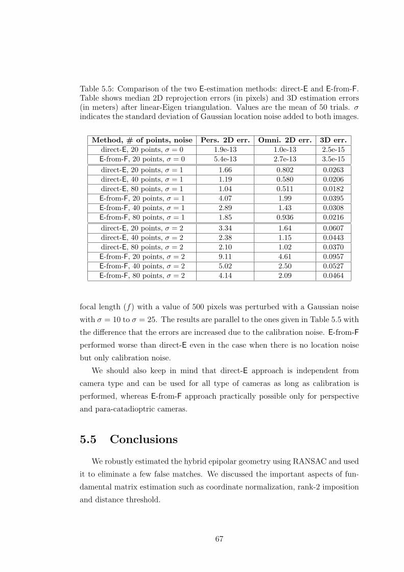
Table 5.5: Comparison of the two E-estimation methods: direct-E and E-from-F.Table shows median 2D reprojection errors (in pixels) and 3D estimation errors(in meters) after linear-Eigen triangulation. Values are the mean of 50 trials. σindicates the standard deviation of Gaussian location noise added to both images.

Method, # of points, noise Pers. 2D err. Omni. 2D err. 3D err.direct-E, 20 points, σ = 0 1.9e-13 1.0e-13 2.5e-15E-from-F, 20 points, σ = 0 5.4e-13 2.7e-13 3.5e-15direct-E, 20 points, σ = 1 1.66 0.802 0.0263direct-E, 40 points, σ = 1 1.19 0.580 0.0206direct-E, 80 points, σ = 1 1.04 0.511 0.0182E-from-F, 20 points, σ = 1 4.07 1.99 0.0395E-from-F, 40 points, σ = 1 2.89 1.43 0.0308E-from-F, 80 points, σ = 1 1.85 0.936 0.0216direct-E, 20 points, σ = 2 3.34 1.64 0.0607direct-E, 40 points, σ = 2 2.38 1.15 0.0443direct-E, 80 points, σ = 2 2.10 1.02 0.0370E-from-F, 20 points, σ = 2 9.11 4.61 0.0957E-from-F, 40 points, σ = 2 5.02 2.50 0.0527E-from-F, 80 points, σ = 2 4.14 2.09 0.0464

focal length (f) with a value of 500 pixels was perturbed with a Gaussian noise

with σ = 10 to σ = 25. The results are parallel to the ones given in Table 5.5 with

the difference that the errors are increased due to the calibration noise. E-from-F

performed worse than direct-E even in the case when there is no location noise

but only calibration noise.

We should also keep in mind that direct-E approach is independent from

camera type and can be used for all type of cameras as long as calibration is

performed, whereas E-from-F approach practically possible only for perspective

and para-catadioptric cameras.

5.5 Conclusions

We robustly estimated the hybrid epipolar geometry using RANSAC and used

it to eliminate a few false matches. We discussed the important aspects of fun-

damental matrix estimation such as coordinate normalization, rank-2 imposition

and distance threshold.

67

We defined normalization matrices for lifted coordinates and performed anal-

ysis on the effectiveness of coordinate normalization and to choose the best values

of scale normalization factor for hybrid case. We concluded that, as suggested

for perspective cameras, carrying the origin to the centroid of points and scaling

coordinates so that the average distance of a point to the origin is equal to√

2 is

proper for normalizing point coordinates in omnidirectional camera images.

We also evaluated the alternatives for pose estimation and decided on esti-

mating the essential matrix with the calibrated 3D rays of point correspondences

rather then extracting the essential matrix from fundamental matrix. This con-

clusion is based on both the performance difference observed in the experimental

analysis and the limitations of obtaining E-from-F for hybrid case.

68

chapter 6

Triangulation

Triangulation is the step of estimating 3D coordinates of the matched 2D

points using camera poses. In this chapter, we present the proposed weighting

strategy for iterative linear-Eigen triangulation method and show its effectiveness

in increasing the 3D structure estimation performance with simulated images.

Also, a two-view hybrid SfM experiment is presented in Section 6.3 in order to

evaluate the proposed triangulation approach for real images.

6.1 Weighted Triangulation for Mixed Camera

Images

We generalized iterative linear-Eigen triangulation method for effective use in

a mixed structure-from-motion pipeline. According to the comprehensive study

by Hartley and Sturm [28], iterative linear-Eigen is one of best triangulation

methods for Euclidean reconstruction. It is superior to midpoint method and non-

iterative linear methods especially when 2D error is considered. For projective

reconstruction, polynomial triangulation method performs better, however it was

also mentioned that, although iterative linear-Eigen is not projective invariant its

performance under projective reconstruction is close to that of polynomial trian-

gulation method. Moreover, polynomial method requires a considerable amount

of computation time and not easily generalizable to more than two images.

Let us briefly go over the iterative linear-Eigen method. Let the two corre-

sponding point coordinates be q = (x, y, 1), q′ = (x′, y′, 1) and their projections

are represented by q = PQ , q′ = P′Q. Letting pi denote the ith row of P, Q

satisfies:

69

AQ = 0 where A =

xp3 − p1

yp3 − p2

x′p′3 − p′1

y′p′3 − p′2

(6.1)

For multi-view triangulation, two rows are added to A for each view. Least

square solution is the last column of V in the singular value decomposition A =

UDVT, which is the unit eigenvector corresponding to the smallest eigenvalue

of the matrix ATA. This method is extended by adjusting the weights of rows

iteratively such that reprojection error will be decreased. The weights for the

first and second views are 1p3Q

and 1p′

3Qrespectively [28].

Please note that we employ this method with calibrated 3D rays instead of

raw pixels. Since the projection in omnidirectional cameras can not be expressed

linearly as in perspective cameras, hybrid triangulation can be performed with

the 3D rays outgoing from the effective viewpoints of the cameras.

The perspective cameras in mixed systems tend to have higher resolution

than the omnidirectional ones. To benefit from their resolution, we increased the

weight of rows coming from perspective images. With the mentioned weighting

strategy, we observed improvement in the accuracy of estimated 3D coordinates.

We relate the amount of weighting to three factors: the scale ratio, the distance

to the scene and the position of the object in the omnidirectional image. Let us

examine these one by one.

Since we perform triangulation with the 3D rays, an object in two images with

different focal lengths cover different amount of areas in the images but have same

field of view in the scene. One pixel noise in the zoomed image corresponds to

lower angular error and distance error on the object. In Fig. 6.1a, the case of

doubling the focal length is depicted. If one pixel noise in the left image causes

δ distance error, then same noise in the right image causes 2δ error. In this case,

we need to increase the weight of the zoomed camera, otherwise triangulation

gives equal weight to both of them.

Distance to the scene affects the triangulation with 3D rays. Rays diverge as

the camera comes closer to the scene. Object in the image gets larger but this

should be distinguished from the zoom effect. We depict this case in Fig. 6.1b.

Both cameras have equal focal length values but distance between the camera on

70

(a) (b)

Figure 6.1: Depiction of doubling the focal length and decreasing the camera-scene distance for triangulation on normalized rays, i.e. normalized image plane.On the top row, images are shown with the object observed. Bottom row showsthe field of view of the camera (top and bottom 3D rays) corresponding to theobject and the distance error on the object (δ or 2δ) corresponding to one pixelerror in the images. C represents the camera center (i.e. pinhole). Dashed linerepresents the normalized image plane. Iterative linear triangulation on 3D raysminimizes the error on that plane. (a) Camera on the left has twice the focallength of the camera on the right. Distance between the camera and the sceneis equal for both cameras. (b) Both cameras have equal focal length values butdistance between the camera on the left and the scene is half the distance betweenthe camera on the right and the scene.

the left and the scene is half the distance between the camera on the right and the

scene. Triangulation already gives support to left camera because it minimizes

the reprojection error on the normalized 3D rays. We do not need to increase the

weight.

The third and the last factor is the position of the points in the catadioptric

image. When the objects in the scene have approximately the same height with

the camera, x and y values in the (x, y, 1) form of normalized 3D rays have quite

high values compared to the values in the perspective images. These high values

cause an unwanted support for the rows coming from catadioptric image. When

the objects are below the camera this does not occur. We observed that, for such

elevated objects, i.e. for the points near the periphery of the catadioptric image,

increasing weight of perspective camera improves the results.

To combine the effects in a single weight coefficient, we propose to multiply

the rows of perspective image by s

s = rs · rd · p (6.2)

71

where rs is assigned as the ratio of the scales of the object in perspective and

omnidirectional images repsectively. Please note that this value is not supposed

to be the ratio of focal length values of the cameras. When camera type differs,

focal length ratio is not the ratio of the sizes of object in the images. Distance

ratio is represented by rd and assigned as the ratio of distances to the scene from

perspective and omnidirectional cameras respectively. Approximate information

of camera positions can be used for less controlled image capturing. Finally p

represents the position factor. If objects/points are high and represented at the

periphery of the catadioptric image, we increase p i.e. weight of the perspective

camera. The value of p was chosen emprically from our experiments. Detailed

results of the experiments analyzing various cases are given in Section 6.2.

Please note that for two perspective cameras, triangulation can be performed

with pixels (not with 3D rays) and since the reprojection error in the image is

minimized, the iterative linear triangulation supports the zoomed image without

requiring an extra weighting for the zoomed images. For the distance effect,

becoming closer to the scene is similar to the zoom effect and position of the

point in the image does not have a significant effect for perspective cameras.

6.2 Experiments

In this section, we analyze the improvement for the proposed weighted trian-

gulation approach (cf. Section 6.1) on simulated data. We generated a total of

1000 points that are regularly distributed on a planar grid. We added Gaussian

location noise to all simulated images with σ=2.0 pixels. We define two main

scenarios to distinguish between the cases when observed points are below the

catadioptric camera or at the same horizontal level with the camera. We depicted

these two cases and camera positions in Fig. 6.2. Two of the camera positions

are selected each time also with varying focal length values to create analyzed

scale ratios.

For the case that the grid is below the catadioptric camera, we have four

experiments, results of which are given in Table 6.1. Camera positions, scale

ratios (rs) and distance ratios w.r.t. the grid (rd) are indicated in the table.

Error is expressed by the median 3D estimation error. Fig. 6.3 shows the images

of the experiment in the first row of Table 6.1 as an example. Applied weight

72

(a) (b)

Figure 6.2: Camera and grid positions in the scene of triangulation experiments.(a) The grid is below the catadioptric camera, side view. (b) The grid is at thesame horizontal level with the cameras, top view. Distance between the camerasis 2 meters. Maximum distance between the cameras and the scene (2l) is 2.5meters.

Table 6.1: Results of triangulation experiments for the scene given in Fig. 6.2a.Error is expressed by 3D coordinate estimation error in meters, median of 1000points in the grid. Experiments were repeated 30 times and the values in thetable are the mean of these 30 experiments. Gaussian location noise with σ=2.0pixels was added to both images.

pair rs rd w = 1 w = s improvementOmni1-Pers1 2 1 0.0250 0.0242 3.2%Omni1-Pers1 4 1 0.0334 0.0302 9.6%Omni1-Pers2 2 0.5 0.0200 0.0200 -Omni2-Pers1 1 2 0.0170 0.0166 2.4%

value is represented with w. Errors for w = 1 and w = s are compared in the

table, where s is calculated by Eq. 6.2 and p = 1 for the current case. We

observe that proposed weighting (s) produces better results. We expressed the

improvement as percentage of decrease in error. Improvement becomes significant

when rs increases which is quite likely for hybrid pairs. For Omni1-Pers2 case, the

effects of rs and rd cancel each other and s = 1 already. We put this experiment

to indicate the importance of rd because we tested with our experiments that

w = 1 is better than w = 2.

When the grid is close to the same horizontal level with the camera (Fig.

6.2b) we again conducted the same experiments, results of which are given in

Table 6.2. This time p 6= 1 due to the position of grid w.r.t. the catadioptric

camera. We observed in our experiments that p = 2 is the best performer for

73

(a) (b)

Figure 6.3: Simulated hybrid image pair of the experiment in the first row ofTable 6.1. (a) perspective image, (b) omnidirectional image.

Table 6.2: Results of triangulation experiments for the scene given in Fig. 6.2b.Error is expressed by 3D coordinate estimation error in meters, median of 1000points in the grid. Experiments were repeated 30 times and the values in thetable are the mean of these 30 experiments. Gaussian location noise with σ=2.0pixels was added to both images.

pair rs rd p w = 1 w = s improvementOmni1-Pers1 2 1 2 0.0266 0.0254 4.5%Omni1-Pers1 4 1 2 0.0317 0.0288 9.2%Omni1-Pers2 2 0.5 2 0.0221 0.0216 2.3%Omni2-Pers1 1 2 2 0.0171 0.0162 5.3%Omni1-Pers1 2 1 1 0.0266 0.0261 1.9%Omni1-Pers1 4 1 1 0.0317 0.0298 6.0%Omni1-Pers2 2 0.5 1 0.0221 0.0221 -Omni2-Pers1 1 2 1 0.0171 0.0167 2.3%

this case and increasing p further does not improve the results. The table also

shows the results for p = 1 which is the case neglecting the position factor. Please

compare the improvements in the top four and bottom four rows to observe the

difference gained by including position factor.

When the observed scene points are below the horizontal level of the cata-

dioptric camera but not directly below (a case between Fig. 6.2a and Fig. 6.2b),

it is appropriate to increase p from 1 to 2 gradually as the 3D points get higher.

The value of p can be assigned according to the vertical angles of the 3D rays

corresponding to the points as demonstrated in the experiment in Section 6.3.

74

6.3 Structure-from-Motion with Real Images

In this section, with the experience gained by the experiments performed for

steps of point matching, pose estimation and triangulation, we choose the best

performing methods and complete a SfM experiment with a real hybrid image

pair.

We estimate the essential matrix with the calibrated rays of point correspon-

dences selected by RANSAC. We use the RANSAC output for Pers2 σ1.5 - VCP1

pair (refer to Table 5.4), which has 70 correspondences. We employ the proposed

weighted iterative linear-Eigen triangulation. In Fig. 6.4, at the top row, we see

the correspondences selected by RANSAC, at the bottom row we observe 2D side-

view (left) and 2D top-view (right) of the reconstructed scene, where Op and Oc

shows perspective and catadioptric camera centers, (Xp,Yp,Zp) and (Xc,Yc,Zc)

shows perspective and catadioptric camera axes, respectively.

For triangulation, we employ weighted approach and compute w with s =

rs · rd · p consulting to the results of Section 6.2. We take rs=1.65 which was

already extracted in point matching step for the current image pair (Section 4.3,

Table 5.4). We know that rd ≈ 2 since we set up the experiment environment,

however one can also use the result of an initial triangulation (like Fig. 6.4 bottom

row) to obtain an approximate ratio of distances to the scene. We employ varying

p values for the points according to the vertical angles of their corresponding 3D

rays. The vertical angles change between 50-90 (0 indicates directly below the

omnidirectional camera) and we take p gradually increasing from 1.5 to 2 with

the increasing angle.

To estimate the improvement gained by the proposed weighting scheme, we

compare a number of real world distances with the ones in the estimated 3D

structure. We measured 30 distances at the real scene corresponding to the

distances between estimated 3D points. They are not in the same scale, thus we

equalized the scale of the distances using the ratio between the averages of 30

distances. We measure the accuracy with the absolute difference of the distances

at the real scene and at the reconstructed scene. Table 6.3 shows the median

of these 30 distance errors (in centimeters) for w = 1 and w = s. One can

see the improvement brought by employing the proposed weighting scheme. For

reference, these 30 measured distances vary between 11.2 cm. and 31.8 cm. having

75

Table 6.3: Distance estimate errors after triangulation for hybrid real image pair.Error is expressed with the absolute difference between the measured real-worlddistances and the estimated distances after triangulation (in centimeters). Valuesare the median of 30 distance errors.

rs rd p w = 1 w = s improvement1.65 2 1.5-2 0.88 0.83 5.7%

a median value of 16.5 cm. and standard deviation of 5.0 cm. The distance error

obtained by the proposed approach has a median value of 0.83 cm. (indicated in

the table) and standard deviation of 0.69 cm. varying between 0.42 and 3.2 cm.

6.4 Conclusions

The work presented in this chapter aimed to achieve more accurate triangula-

tion for hybrid camera images and based on the fact that the significant resolution

difference between omnidirectional and perspective images should be considered.

We chose the iterative linear-Eigen triangulation method since it is superior

to midpoint method and non-iterative linear methods and one of the best al-

ternatives for Euclidean reconstruction. We developed a weighting strategy by

analyzing the factors affecting the 3D estimation accuracy and showed its effec-

tiveness with simulated images. We also presented a two-view hybrid SfM exper-

iment and demonstrated the improvement gained by the weighted triangulation

approach with an analysis on distance estimation errors.

76

Figure 6.4: Reconstruction with hybrid real image pair. Selected correspondenceson images are viewed on top. Images are cropped to make points distinguishable.At the bottom row, 2D side-view (left) and 2D top-view (right) of the recon-structed scene can be observed.

77

chapter 7

Multi-view SfM

This chapter presents the work on multi-view Structure-from-Motion (SfM)

with hybrid images. We start by describing the approach we employ to integrate

additional views for multi-view SfM (Section 7.1). The implementation of sparse

bundle adjustment and the improvement it provides are discussed in Section

7.2. One of the main motivations in this thesis is presented with the theory

and experiment given in Section 7.3 where the structures estimated with two

perspective cameras with no view in common are combined by pairing them with

an omnidirectional camera.

7.1 Computing the Projection Matrices of Ad-

ditional Views

To integrate additional views for multi-view SfM, we employed the approach

proposed by Beardsley et al. [29]. In this approach, when a sequence of views is

available, initially SfM is applied for the first two views. Then, for each new view

i, feature detection and matching is applied to establish 2D correspondences with

the previous view i − 1, which are then matched with the already constructed

3D points. The projection matrix of the new view is computed using these final

2D-3D matches as explained below.

Let the 2D-3D matches are represented by xi and Xi, respectively. Projection

can be written as xi = PXi where

xi =

wixi

wiyi

wi

78

and

Xi =

Xi

Yi

Zi

1

This leads to three equations per 2D-3D match to solve for P:

wixi = pT1 Xi

wiyi = pT2 Xi

wi = pT3 Xi

where pTk represents the kth row of P. However, we need to eliminate the unknown

scale factor w. Thus, we write the two equations below:

pT1 Xi − xipT

3 Xi = 0

pT2 Xi − yipT

3 Xi = 0

When represented as a matrix multiplication:

(Xi

T 0T xiXiT

0T XiT yiXi

T

)p1

p2

p3

= 0.

We stack the equations for n points (2 per correspondence) and obtain a

2nx12 matrix A which holds Ap = 0 where p is the column vector containing

the elements of P. We compute the least-squares solution of p by singular value

decomposition (SVD).

Lastly, 3D coordinates of the newly matched 2D points are computed with

triangulation and they are added to the structure.

Multi-view SfM with Projective Factorization. We would like to briefly

describe an alternative approach used for multi-view structure computation and

explain why it is not suitable to be used for our problem. This approach is widely

referred as projective factorization and constructs a measurement matrix which

79

contains the projections of all 3D points in all cameras:w1

1x11 w1

2x12 · · · w1

nx1n

.... . .

...

wm1 xm1 wm2 xm2 · · · wmn xmn

=

P1

...

Pm

(X1 · · · Xn

)(7.1)

where i = 1, ..,m denotes images and p = 1, .., n denotes points. Xp are the

homogeneous coordinate vectors of the 3D points, Pi are the unknown 3x4 pro-

jection matrices, xip are the measured homogeneous coordinate vectors of the

image points and wip are the unknown scale factors since projection of Xp is

defined up to scale:

wipxip = PiXp (7.2)

The measurement matrix can be approximated to its nearest rank-4 form

by using SVD and when decomposed into UDVT, (P1T,P2T

, ..,PmT)T

= UD and

(X1,X2, ..,Xn) = VT. Please note that this factorization is not unique and this

makes the result of the method always a projective reconstruction even if the

cameras are calibrated. Thus, conversion to an Euclidean reconstruction should

be performed using additional methods.

The original algorithm proposed by Sturm and Triggs [64] requires all points

are available in all frames. Later on, this approach was improved to handle

occlusions up to an extent [65]. The proposed improvement uses the available

measurements to fill the missing entries of the measurement matrix and image

sequence should have an amount of coverage in terms of tracked points. The

degradation of reconstruction with decreasing amount of coverage is discussed

in [66] where upgrading the projective reconstruction to an Euclidean one is also

demonstrated.

In addition to these two reasons, projective reconstruction and the sparse-

ness of the measurement matrix, factorization based multi-view approach is not

suitable for our problem of merging hybrid reconstructions due to the fact that

projection of omnidirectional images can not be written in a linear fashion to-

gether with the perspective images as given in Eq. 7.2.

80

7.2 Sparse Bundle Adjustment

Sparse bundle adjustment method proposed by Lourakis and Argyros [30]

has become popular in the community due to its capability of solving enormous

minimization problems (with many cameras and 3D points) in a reasonable time.

We employed this method for our system of mixed cameras. We modified the

projection function with the sphere model projection and intrinsic parameters

with sphere model parameters to encompass the mixed camera types. The details

of sphere model projection was presented in Section 2.2.

7.2.1 Experiment

We conducted a real image hybrid multi-view experiment and refined the re-

sults with sparse bundle adjustment (SBA). Thus we completed the entire pipeline

of hybrid SfM which was shown in Fig. 1.1. Views Pers1-Pers2-Pers3 and Omni1

in Fig. 4.7 were used. Initial structure estimation was performed with Pers1-Pers2

pair, then Pers3 and Omni1 views were added. 75 feature points are common in

all the images. Estimated coordinates of these points and estimated camera po-

sitions are shown in Fig. 7.1.

We performed SBA on this structure (scene point coordinates) and camera

parameters. The reprojection errors before and after SBA (in pixels) are given

in Table 7.1. We infer from the table that the reprojection errors are consider-

ably decreased after SBA. The error before SBA for the omnidirectional image

is higher than the perspective images. This is mainly due to the fact that the

number of common points between omnidirectional and perspective images is less

when compared to the number of common feature points between two perspective

images, which decreases the accuracy of pose estimation. When adding a per-

spective camera to the structure, the projection matrix (extrinsic parameters) of

this new camera is computed by available 2D-3D correspondences (usually more

than 500 points), however when an omnidirectional camera is added, there are

less (usually less than 100 points) number of 2D-3D correspondences to compute

its extrinsic parameters.

81

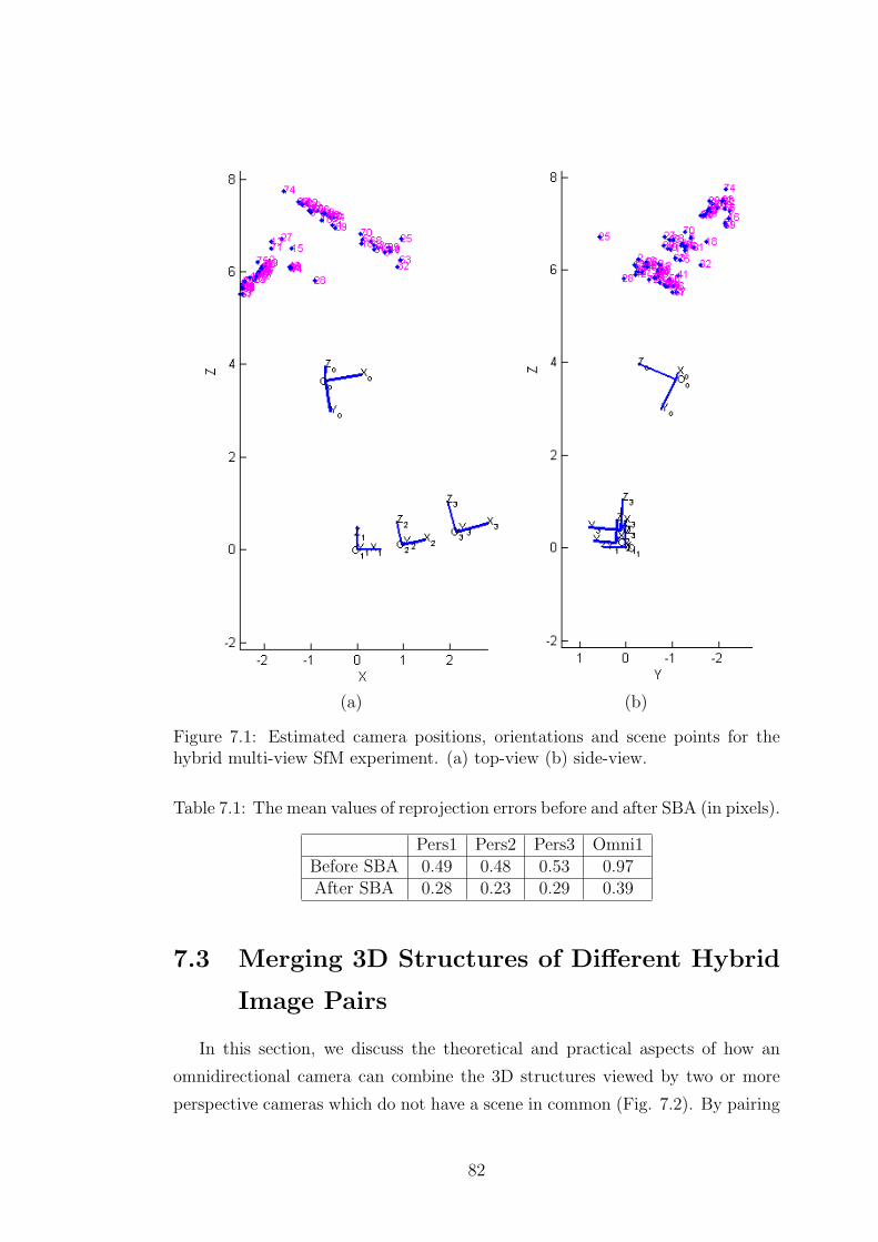
(a) (b)

Figure 7.1: Estimated camera positions, orientations and scene points for thehybrid multi-view SfM experiment. (a) top-view (b) side-view.

Table 7.1: The mean values of reprojection errors before and after SBA (in pixels).

Pers1 Pers2 Pers3 Omni1Before SBA 0.49 0.48 0.53 0.97After SBA 0.28 0.23 0.29 0.39

7.3 Merging 3D Structures of Different Hybrid

Image Pairs

In this section, we discuss the theoretical and practical aspects of how an

omnidirectional camera can combine the 3D structures viewed by two or more

perspective cameras which do not have a scene in common (Fig. 7.2). By pairing

82

Figure 7.2: Depiction of merging 3D structures estimated with different hybridimage pairs.

Figure 7.3: Depiction of aligning and scaling the 2nd 3D structure w.r.t. the firstone to obtain a combined structure.

the perspective views with the same omnidirectional view, it is possible to combine

the 3D structures estimated with different hybrid image pairs. This is one of

the main motivations in this thesis since it is not possible to combine different

perspective cameras if they do not view the same scene. It is even very difficult

if they share a small portion of the view because epipolar geometry estimation

becomes inaccurate and if the correspondence points lie on a planar surface it

becomes totally impossible.

The multi-view approach described in Section 7.1 does not allow us to obtain

a combined structure from these two hybrid pairs directly. When we perform SfM

for two hybrid pairs, we obtain two 3D structures which are in different scales

because the generated structures are true up to a scale factor. Therefore, first we

83

have to align the two structures using the rotation and translation of the common

view, second we have to adjust the scale by estimating or defining the true ratio

of scales. These alignment and scaling processes are depicted in Fig. 7.3 and

briefly described in the following.

Let (R12,t12) be the rotation and translation between the first perspective

image and the omnidirectional image, and (R23,t23) be the ones between the om-

nidirectional image and the other perspective image. When the center of the

first perspective camera is taken as the origin of coordinate system, the exter-

nal calibration matrix of the second camera (omnidirectional camera) becomes

Kext,2 = [R12 | t12].

The rotation of the third camera (2nd perspective image) in the same coordi-

nate system can easily be defined as the multiplication of rotations:

R13 = R23 · R12

The translation vector of the third camera can be formulated as the translation

between second and third cameras in addition to the translation between first two

cameras when rotated with R23 to be represented w.r.t. the third camera:

t13 = t23 + R23 · t12

As a result, the external calibration matrix of the second perspective image

is as below. The origin is still the center of the first camera.

Kext,3 = [R13 | t13]

However, as we have mentioned earlier, the scales of these two motions are

not necessarily the same. To obtain the structure as a whole, we need to estimate

the ratio of scales and adjust the scale of the second structure by multiplying

the translation vector by this ratio. In the following experiment, benefiting from

the small overlap between two perspective images, to estimate the scale ratio we

used the 3D points which are available in both reconstructions. We minimized

the distance between these points in the two reconstructions.

If there is no overlap, knowledge of real world distances in the scene or the

distance between the camera pair can be used to obtain the true scale ratio.

84

7.3.1 Experiment

In Fig. 7.4, on the top row, we observe two perspective images, which have

little intersection in their field of view. At the bottom-left, the omnidirectional

view is seen in which 2D points matched with perspective images are indicated

with different colors. Finally, at the bottom-left, we see the top-view of the

estimated structure. Along with the reconstructed 3D points we also observe the

positions, orientations and field of views of the cameras. The circle around the

middle camera indicates the 360 field of view. 71 points are common between

left perspective view and omnidirectional view, whereas 124 points are common

in the right hybrid pair. Only four of these feature points are common in all three

images.

As mentioned, the scales of the two structures estimated by the hybrid pairs

are not the same and to align these two reconstructed sections we used the four

3D points which are available in both reconstructions. In ideal case, when the

structures are perfectly aligned, the distances from these points to the origin

should be equal in both structures. When imperfections exist, however, the dif-

ference of distances is not zero. We seek for the best scale ratio that minimizes

this distance error. With the scale ratio corresponding to the minimum error, it

is assumed that the best possible alignment is obtained.

The estimated scale ratio is 0.334 for our experiment. In the 3D structure

given in Fig. 7.4 (bottom-left), the structure estimated by the right hand side

perspective camera and omnidirectional camera is downscaled with this ratio.

7.4 Conclusions

In this chapter, we explained our work on multi-view hybrid Structure-from-

Motion. We employed the approach proposed by Beardsley et al. [29] in which

the initial structure is estimated with the first two views and additional views are

added to the structure via 3D-2D correspondences between structure and new

view. This approach seems to be the only option for multi-view hybrid SfM since

the other option used for perspective cameras, projective factorization, can not be

applied to our case due to the fact that the projection of omnidirectional images

can not be written linearly together with the perspective images. It may be

85

Figure 7.4: Matched points between the perspective images (top row) and om-nidirectional image (bottom-left) and the estimated structure (bottom-right) forthe experiment of merging 3D structures.

86

possible to employ lifted coordinates and write 6x10 generic projection matrices

for all points as described in Section 3.2.2 to represent the projections linearly

and form Eq. 7.1. However it would be impractical since the number of unknowns

increase five-fold for camera parameters and three-fold for point coordinates.

We employed sparse bundle adjustment method by modifying the projection

function with sphere model projection and intrinsic parameters with sphere model

parameters. The improvement gained by bundle adjustment is demonstrated with

an experiment of multi-view hybrid SfM. Thus, the complete pipeline of hybrid

SfM, given in Fig. 1.1, is realized.

One of the main motivations in this thesis is presented with the theory and

experiment given in Section 7.3 where the structures estimated with two perspec-

tive cameras which do not view the same part of the scene can be combined by

pairing them with an omnidirectional camera.

87

chapter 8

Conclusions

In this thesis, theoretical and practical issues concerning structure-from-motion

(SfM) with mixed camera images are investigated in detail. The work is moti-

vated by the possible advantages of employing omnidirectional and perspective

cameras together. An example scenario is the usage of an omnidirectional cam-

era with several perspective cameras (or several views of a perspective camera)

which do not necessarily have a view in common. Such a scenario occurs when

the cameras are located at the central region and view the perimeter. Omni-

directional view is able to combine partial 3D structures obtained by different

omnidirectional-perspective image pairs. Otherwise, 3D reconstruction with only

perspective cameras requires a large number of cameras.

Surveillance is another potential application area. Hybrid systems were pro-

posed where slave pan-tilt-zoom cameras are directed according to the infor-

mation obtained by an omnidirectional camera which performs event detection.

Such systems can be enhanced by adding 3D structure and location estimation

algorithms without increasing the number of cameras.

We described an end-to-end pipeline for hybrid multi-view structure-from-

motion and proposed new approaches or modified existing methods for the steps

of this pipeline which can be summarized as camera calibration, feature point

matching, epipolar geometry and pose estimation, triangulation and bundle ad-

justment.

We employed the sphere camera model [25] to represent mixed types of cam-

eras. We did not need to change the camera model for different camera pairs or

between SfM steps.

We presented a calibration technique based on the sphere camera model which

is able to represent every single-viewpoint catadioptric system. We tested this

method both with simulations and real images. When compared to previous

techniques of sphere model calibration, our method has the advantages of not

88

requiring input for parameter initialization and being able to calibrate perspective

cameras as well. On the other hand, it needs a 3D calibration object.

It had been stated that directly applying SIFT [21] is not sufficient to obtain

good results for hybrid image pairs. In our study, we showed that the performance

of SIFT considerably increases with the proposed algorithm of low-pass filtering

and downsampling the perspective image in the hybrid pair. Another approach we

evaluate is generating virtual camera plane (VCP) image from the omnidirectional

image first and then applying SIFT. We conducted experiments with two different

catadioptric cameras and a fish-eye camera. We observed that VCP approach

performed best for catadioptric images and is more robust to increasing baseline.

For fish-eye images, preprocessing without VCP approach performed as well as

the VCP approach due to the fact that a fish-eye camera looking towards the

scene acts as a perspective camera with a large lens distortion and serves as a

good candidate for matching with perspective cameras.

The proposed algorithm for feature point matching brings the advantage of au-

tomatic point matching between omnidirectional and perspective images. More-

over, we are able to say that the proposed technique of extracting parameters

of low-pass filtering and downsampling is versatile up to a large extent since it

worked in our experiments with three different omnidirectional cameras.

The proposed point matching algorithm should not be considered as a false

match elimination technique since it increases the performance at the matching

stage. Thus, it is not compensated by elimination techniques such as the one

proposed by Lowe [21] which eliminates matches that do not conform to an affine

transformation. On the other hand, employing such an elimination together with

the proposed technique has the potential of improving the result especially for

VCP-perspective matching. We did not integrate such a step since next step

in our pipeline is the estimation of hybrid epipolar geometry and elimination of

matches that do not conform to the epipolar geometry which is a more accurate

geometrical constraint.

We robustly estimated the hybrid epipolar geometry using RANSAC. We

discussed the important aspects of fundamental matrix estimation such as co-

ordinate normalization, rank-2 imposition and distance threshold. We defined

normalization matrices for lifted coordinates and performed detailed analysis on

the effectiveness of coordinate normalization and choosing the best values of scale

89

normalization factor for hybrid case. We concluded that, as suggested for perspec-

tive cameras, carrying the origin to the centroid of points and scaling coordinates

so that the average distance of a point to the origin is equal to√

2 is proper for

normalizing point coordinates in omnidirectional camera images.

We also evaluated the alternatives for pose estimation and decided on esti-

mating the essential matrix with the calibrated 3D rays of point correspondences

rather than extracting the essential matrix from fundamental matrix. This de-

cision is based on both the performance difference observed in the experimental

analysis and the limitations of obtaining E from F for hybrid systems with cata-

dioptric cameras with hyperbolic mirrors.

Aiming to achieve more accurate triangulation for hybrid camera images and

based on the fact that the significant resolution difference between omnidirec-

tional and perspective images should be considered, we proposed a weighting

strategy for iterative linear-Eigen triangulation method. We showed its effective-

ness with simulated images and real image hybrid SfM experiment.

For multi-view hybrid SfM, we implemented the approach proposed by Beard-

sley et al. [29] in which the initial structure is estimated with the first two views

and additional views are added to the structure via 3D-2D correspondences be-

tween the structure and the new view. This approach seems to be the only option

for multi-view hybrid SfM since the other option used for perspective cameras,

projective factorization, can not be applied to our case due to the fact that the

projection of omnidirectional images can not be written linearly together with

the perspective images.

We employed the sparse bundle adjustment method [30] by modifying the pro-

jection function with the sphere model projection and intrinsic parameters with

the sphere model parameters. The improvement gained by bundle adjustment

was demonstrated with an experiment of hybrid multi-view SfM.

In conclusion, with the suggested techniques and proposed improvements in

this thesis, it is possible to perform hybrid multi-view structure-from-motion in

an effective and automatic way.

90

8.1 Limitations and Future Work

The presented calibration method was tested with simulated and real images

of catadioptric cameras. Although we left it as a future work, it may be possi-

ble to generalize the algorithm to cover the fish-eye cameras as well. Ying and

Hu [53] showed that the sphere model can approximate fisheye projections and

Hansen et al. [57] employed this approach. The hybrid epipolar geometry and

pose estimation steps can also be performed for fish-eye cameras as the theory

was given in [18]. Sparse bundle adjustment can be directly applied for fish-eye

cameras by modifying its projection function accordingly.

The optimal scale ratio detection and preprocessing the high-resolution image

approach proposed in this work can be used for other applications employing

SIFT where an approximate scale ratio exists between the objects in the given

images. Otherwise, if scale ratios considerably vary for objects in the scene, this

approach is not suitable.

Another approach to detect and match scale-invariant features for omnidirec-

tional cameras was proposed by Hansen et al. [57] where features are detected in

the spherical domain. When compared to the conventional SIFT applied on 2D

image plane, it brought improvement for some camera types and in certain mo-

tion scenarios. This is a new approach and may lead to better results in the near

future. Therefore, integrating or comparing the proposed preprocessing method

with this “SIFT on Sphere” approach may be beneficial.

91

references

[1] Chahl, J. and Srinivasan, M., 2000. A Complete Panoramic Vision Sys-tem, Incorporating Imaging, Ranging, and Three Dimensional Navigation,Proc. of IEEE Workshop on Omnidirectional Vision (OMNIVIS), pp. 104–111.

[2] Gaspar, J., Winters, N. and Santos-Victor, J., 2000. Vision-BasedNavigation and Environmental Representations with an OmnidirectionalCamera, IEEE Transactions on Robotics and Automation, 16(6), 890–898.

[3] Ng, K., Ishiguro, H., Trivedi, M. and Sogo, T., 2004. An IntegratedSurveillance System: Human Tracking and View Synthesis using MultipleOmni-directional Vision Sensors, Image and Vision Computing, 22, 551–561.

[4] Cui, Y., Samarasekera, S., Huang, Q. and Greiffenhagen, M., 1998.Indoor Monitoring via the Collaboration between a Peripheral Sensor and aFoveal Sensor, IEEE Workshop on Visual Surveillance, pp. 2–9.

[5] Yao, Y., Abidi, B. and Abidi, M., 2006. Fusion of Omnidirectional andPTZ Cameras for Accurate Cooperative Tracking, IEEE Int. Conference onVideo and Signal Based Surveillance (AVSS).

[6] Scotti, G., Marcenaro, L., Coelho, C., Selvaggi, F. and Regazzoni,C., 2005. Dual Camera Intelligent Sensor for High Definition 360 DegreesSurveillance, IEE Proc.-Vision Image Signal Processing, 152(2), 250–257.

[7] Fleck, S., Busch, F., Biber, P., Andreasson, H. and Strasser,W., 2005. Omnidirectional 3D Modeling on a Mobile Robot using GraphCuts, Proc. of IEEE International Conference on Robotics and Automation(ICRA), pp. 1748–1754.

[8] Lhuillier, M., 2007. Toward Flexible 3D Modeling using a CatadioptricCamera, IEEE Conf. on Computer Vision and Pattern Recognition (CVPR).

[9] Chang, P. and Hebert, M., 2000. Omni-directional Structure from Mo-tion, Proc. of IEEE Workshop on Omnidirectional Vision (OMNIVIS), pp.127–133.

[10] Hartley, R. and Zisserman, A., 2004. Multiple View Geometry in Com-puter Vision, Cambridge Univ. Press, 2nd edition.

92

[11] Lhuillier, M., 2005. Automatic Structure and Motion using a CatadioptricCamera, Workshop on Omnidirectional Vision, Camera Networks and Non-classical Cameras (OMNIVIS).

[12] Bunschoten, R. and Krose, B., 2003. Robust Scene Reconstruction froman Omnidirectional Vision System, IEEE Transactions on Robotics and Au-tomation, 19(2), 351–357.

[13] Micusik, B. and Pajdla, T., 2006. Structure from Motion with WideCircular Field of View Cameras, IEEE Transactions on Pattern Analysisand Machine Intelligence, 28(7), 1135–1149.

[14] Chen, X., Yang, J. and Waibel, A., 2003. Calibration of a Hybrid Cam-era Network, Proc. of IEEE International Conference on Computer Vision(ICCV), pp. 150–155.

[15] Adorni, G., Cagnoni, S., Mordonini, M. and Sgorbissa, A., 2003.Omnidirectional Stereo Systems for Robot Navigation, Proc. of Workshopon Omnidirectional Vision and Camera Networks (OMNIVIS).

[16] Chen, D. and Yang, J., 2005. Image Registration with Uncalibrated Cam-eras in Hybrid Vision Systems, IEEE Workshop on Application of ComputerVision, pp. 427–432.

[17] Sturm, P., 2002. Mixing Catadioptric and Perspective Cameras, Proc. ofWorkshop on Omnidirectional Vision (OMNIVIS), pp. 37–44.

[18] Barreto, J. and Daniilidis, K., 2006. Epipolar Geometry of Central Pro-jection Systems using Veronese Maps, Int. Conference on Computer Visionand Pattern Recognition (CVPR), pp. 1258–1265.

[19] Sturm, P. and Barreto, J., 2008. General Imaging Geometry for CentralCatadioptric Cameras, European Conference on Computer Vision (ECCV),pp. 609–622.

[20] Puig, L., Guerrero, J. and Sturm, P., 2008. Matching of Omnidirec-tional and Perspective Images using the Hydrid Fundamental Matrix, Proc.of Workshop on Omnidirectional Vision (OMNIVIS).

[21] Lowe, D., 2004. Distinctive Image Features from Scale Invariant Keypoints,International Journal of Computer Vision, 60, 91–110.

[22] Fischler, M. and Bolles, R., 1981. Random Sample Consensus: AParadigm for Model Fitting with Applications to Image Analysis and Auto-mated Cartography, Communications of the ACM, 24(6), 381–395.

[23] Ramalingam, S., Lodha, S. and Sturm, P., 2004. A Generic Structure-from-motion Algorithm for Cross-camera Scenarios, Proc. of IEEE Workshopon Omnidirectional Vision (OMNIVIS), pp. 175–186.

93

[24] Sturm, P. and Ramalingam, S., 2004. A Generic Concept for CameraCalibration, European Conference on Computer Vision (ECCV), pp. 1–13.

[25] Geyer, C. and Daniilidis, K., 2000. A Unifying Theory for CentralPanoramic Systems, European Conference on Computer Vision (ECCV),pp. 445–461.

[26] Mei, C. and Rives, P., 2007. Single Viewpoint Omnidirectional CameraCalibration from Planar Grids, IEEE International Conference on Roboticsand Automation (ICRA), pp. 3945–3950.

[27] Matas, J., Chum, O., Urban, M. and Pajdla, T., 2002. Robust WideBaseline Stereo from Maximally Stable Extremal Regions, Proc. of BritishMachine Vision Conference (BMVC), pp. 384–393.

[28] Hartley, R. and Sturm, P., 1997. Triangulation, Computer Vision andImage Understanding, 68(2), 146–157.

[29] Beardsley, P., Zisserman, A. and Murray, D., 1997. Sequential Updat-ing of Projective and Affine Structure from Motion, IJCV, 23(3), 235–259.

[30] Lourakis, M. and Argyros, A., 2004, The Design and Implementationof a Generic Sparse Bundle Adjustment Software Package based on the LMAlgorithm, FORTH-ICS Technical Report, TR-340.

[31] Rees, D., 1970. Panoramic Television Viewing System, US Patent No.3505465.

[32] Nayar, S. and Peri, V., 1999, Folded Catadioptric Cameras, TechnicalReport, Dept. of Computer Science, Columbia University.

[33] Conroy, T. and Moore, J., 1999. Resolution Invariant Surfaces forPanoramic Vision Systems, Proc. of IEEE International Conference on Com-puter Vision (ICCV), pp. 392–397.

[34] Hicks, R. and Bajcsy, R., 2000. Catadioptric Sensors that ApproximateWide-Angle Perspective Projections, Proc. of IEEE Workshop on Omnidi-rectional Vision (OMNIVIS), pp. 97–103.

[35] Gaspar, J., Decc, C., Okamoto, J. and Santos-Victor, J., 2002. Con-stant Resolution Omnidirectional Cameras, Proc. of IEEE Workshop on Om-nidirectional Vision (OMNIVIS), pp. 27–36.

[36] Swaminathan, R., Grossberg, M. and Nayar, S., 2004. Designing Mir-rors for Catadioptric Systems that Minimize Image Errors, Proc. of IEEEWorkshop on Omnidirectional Vision (OMNIVIS), pp. 91–102.

[37] Baker, S. and Nayar, S., 1999. A Theory of Single-viewpoint CatadioptricImage Formation, IJCV, 35(2), 175–196.

94

[38] Swaminathan, R., Grossberg, M. and Nayar, S., 2001, Non Single-viewpoint Catadioptric Cameras, Technical Report, Department of Com-puter Science, Columbia University.

[39] Derrien, S. and Konolige, K., 2000. Approximating a Single-viewpoint inPanoramic Imaging Devices, Proc. of Workshop on Omnidirectional Vision(OMNIVIS), pp. 85–90.

[40] Ho, T., Davis, C. and Milner, S., 2005. Using Geometric Constraints forFisheye Camera Calibration, Proc. of Workshop on Omnidirectional Vision(OMNIVIS).

[41] Barreto, J. and Araujo, H., 2005. Geometric Properties of Central Cata-dioptric Line Images and Their Application in Calibration, IEEE Transac-tions on Pattern Analysis and Machine Intelligence, 27(8), 1327–1333.

[42] Geyer, C. and Daniilidis, K., 2002. Paracatadioptric Camera Calibration,IEEE Transactions on Pattern Analysis and Machine Intelligence, 24(5),687–695.

[43] Kang, S., 2000. Catadioptric Self-calibration, Int. Conference on ComputerVision and Pattern Recognition (CVPR), pp. 1201–1207.

[44] Orghidan, R., Salvi, J. and Mouaddib, M., 2003. Calibration of aStructured Light-based Stereo Catadioptric Sensor, Proc. of Workshop onOmnidirectional Vision and Camera Networks (OMNIVIS).

[45] Cauchois, C., Brassart, E. and Drocourt, C., 1999. Calibration of theOmnidirectional Vision Sensor: SYCLOP, IEEE International Conferenceon Robotics and Automation (ICRA), pp. 1287–1292.

[46] Kannala, J. and Brandt, S., 2004. A Generic Camera Calibration Methodfor Fish-eye Lenses, Proc. of International Conference on Pattern Recogni-tion (ICPR), pp. 10–13.

[47] Scaramuzza, D., Martinelli, A. and Siegwart, R., 2006. A Toolbox forEasily Calibrating Omnidirectional Cameras, Int. Conference on IntelligentRobots and Systems (IROS), pp. 5695–5701.

[48] Abdel-Aziz, Y. and Karara, H., 1971. Direct Linear Transformationfrom Comparator Coordinates into Object Space Coordinates in Close-rangePhotogrammetry, Symposium on Close-Range Photogrammetry, pp. 1–18.

[49] Horn, R. and Johnson, C., 1991. Topics in Matrix Analysis, CambridgeUniv. Press, 2nd edition.

[50] Horn, R. and Johnson, C., 1985. Matrix Analysis, Cambridge Univ.Press.

95

[51] Bastanlar, Y., Puig, L., Sturm, P., Guerrero, J. and Barreto, J.,2008. DLT-like Calibration of Central Catadioptric Cameras, Proc. of Work-shop on Omnidirectional Vision (OMNIVIS).

[52] Heikilla, J. and Silven, O., 1997. A Four-step Camera Calibration Pro-cedure with Implicit Image Correction, Proc. of Conference on ComputerVision and Pattern Recognition (CVPR), pp. 1106–1112.

[53] Ying, X. and Hu, Z., 2004. Can We Consider Central Catadioptric Cam-eras and Fisheye Cameras Within a Unified Imaging Model?, European Con-ference on Computer Vision (ECCV), pp. 442–455.

[54] Yi, Z., Zhiguo, C. and Yang, X., 2008. Multi-spectral Remote ImageRegistration based on SIFT, Electronic Letters, 44(2), 107–108.

[55] Alhwarin, F., Wang, C., Ristic-Durrant, D. and Graser, A., 2008.Improved SIFT-Features Matching for Object Recongnition, Visions of Com-puter Science - BCS International Academic Conference.

[56] Peri, V. and Nayar, S., 1997. Generation of Perspective and PanoramicVideo from Omnidirectional Video, Proc. of DARPA Image UnderstandingWorkshop, pp. 243–246.

[57] Hansen, P., Corke, P., Wageeh, B. and Daniilidis, K., 2007. Scale-Invariant Features on the Sphere, IEEE International Conference on Com-puter Vision (ICCV).

[58] Svoboda, T. and Pajdla, T., 2002. Epipolar Geometry for Central Cata-dioptric Cameras, International Journal of Computer Vision, 49, 23–37.

[59] Geyer, C. and Daniilidis, K., 2001. Structure and Motion from Uncali-brated Catadioptric Views, Int. Conference on Computer Vision and PatternRecognition (CVPR), pp. 279–286.

[60] Claus, D. and Fitzgibbon, A., 2005. A Rational Function Lens DistortionModel for Generic Cameras, Int. Conference on Computer Vision and PatternRecognition (CVPR), pp. 213–219.

[61] Fitzgibbon, A., 2001. Simultaneous Linear Estimation of Multiple ViewGeometry and Lens Distortion, IEEE Computer Society Conference on Com-puter Vision and Pattern Recognition (CVPR), volume 1, pp. 125–132.

[62] Hartley, R., 1997. In Defense of the Eight-Point Algorithm, IEEE Trans-actions on Pattern Analysis and Machine Intelligence, 19(6), 580–593.

[63] Bartoli, A. and Sturm, P., 2004. Non-linear Estimation of the Funda-mental Matrix with Minimal Paremeters, IEEE Transactions on PatternAnalysis and Machine Intelligence, 26(3), 426–432.

96

[64] Sturm, P. and Triggs, B., 1996. A Factorization Based Algorithm forMulti-Image Projective Structure and Motion, Proc. of European Conferenceon Computer Vision (ECCV), pp. 709–720.

[65] Martinec, D. and Pajdla, T., 2002. Structure from Many PerspectiveImages with Occlusions, Prof. of European Conference on Computer Vision(ECCV), volume 2, pp. 355–369.

[66] Martinec, D. and Pajdla, T., 2005. 3D Reconstruction by Fitting Low-rank Matrices with Missing Data, IEEE Computer Society Conference onComputer Vision and Pattern Recognition (CVPR), volume 1, pp. 198–205.

97

CURRICULUM VITAE

PERSONAL INFORMATION

Surname, Name: Bastanlar, YalınNationality: TurkishDate of Birth: 21.09.1978Place of Birth: Ankara, TurkeyMarital Status: SingleE-mail: yalinb@yahoo.com

EDUCATION

Degree Institution YearPh.D. in Information Systems Middle East Technical University 2009M.Sc. in Information Systems Middle East Technical University 2005B.Sc. in Civil Engineering Middle East Technical University 2001

WORK EXPERIENCE

Year Place EnrollmentJan.’06 - Sept.’09 Middle East Technical University Research AssistantMar.’08 - Aug.’08 INRIA Rhone-Alpes (France) Visiting ResearcherSept.’04 - Dec.’05 Middle East Technical University Project Researcher

RESEARCH INTERESTS

Catadioptric omnidirectional cameras and image formation processes;Calibration and epipolar geometry of omnidirectional cameras;Structure-from-motion and 3D reconstruction;Corner detection;Usage of 360 in Web-based virtual tours;Human factors and usability in virtual reality applications.

FOREIGN LANGUAGES

English: Very GoodFrench: Intermediate

98

PUBLICATIONS

Journals:

• Bastanlar, Y., Yardimci, Y., Temizel, A., Sturm, P., “Automatic and RobustStructure-from-Motion for Mixed Camera Systems”, submitted to IJCV SpecialIssue on Omnidirectional Vision, Camera Networks and Non-Classical Cameras.• Puig, L., Bastanlar, Y., Sturm, P., Guerrero Campo, J., Barreto, J., “Calibra-tion of Central Catadioptric Cameras Using a DLT-Like Approach”, submittedto IJCV Special Issue on Omnidirectional Vision, Camera Networks and Non-Classical Cameras.• Bastanlar, Y., Yardimci, Y. (2008), “Corner Validation based on ExtractedCorner Properties”, Computer Vision and Image Understanding (CVIU), vol.112,p.243-261.

International Conferences:

• Bastanlar, Y., Puig, L., Sturm, P., Guerrero Campo, J., Barreto, J. (2008),“DLT-like Calibration of Central Catadioptric Cameras”, Proc. of Workshop onOmnidirectional Vision (OmniVis 2008), 12-18 October, Marseille, France.• Bastanlar, Y., Grammalidis, N., Zabulis, X., Yilmaz, E., Yardimci, Y., Tri-antafyllidis, G. (2008), “3D Reconstruction for a Cultural Heritage Virtual TourSystem”, XXI Congress of the International Society for Photogrammetry andRemote Sensing (ISPRS 2008), 3-11 July, Beijing, China.• Zabulis, X., Grammalidis, N., Bastanlar, Y., Yilmaz, E., Yardimci, Y. (2008),“3D Scene Reconstruction Based on Robust Camera Motion Estimation andSpace Sweeping for a Cultural Heritage Virtual Tour System”, 3DTV-Conference,28-30 May, Istanbul, Turkey.• Bastanlar, Y. (2007), “User Behaviour in Web-Based Interactive Virtual Tours”,29th International Conference on Information Technology Interfaces (ITI 2007),25-28 June, Dubrovnik, Croatia.• Bastanlar, Y., Canturk, D., Uke, H. (2007), “Effects of Color-multiplex Stereo-scopic View on Memory and Navigation”, 3DTV-Conference: The True Vision:Capture, Transmission and Display of 3D Video, 7-9 May, Cos, Greece.• Bastanlar, Y., Cetin, A.E., Yardimci, Y. (2005), “Enhancement of PanoramasGenerated from Omnidirectional Images”, International Workshop on SamplingTheory and Applications (SampTA 2005), 10-15 July, Samsun, Turkey.

National Conferences:

• Bastanlar, Y., Temizel, A., Yardimci, Y. (2009), “Automatic Point Match-ing and Robust Fundamental Matrix Estimation for Hybrid Camera Scenarios”,(in Turkish), IEEE National Conference on Signal Processing and Applications(SIU 2009), 9-11 April, Antalya, Turkey.

99

• Serce, H., Bastanlar, Y., Temizel, A., Yardimci, Y. (2008), “On Detection ofEdges and Interest Points for Omnidirectional Images in Spherial Domain” (inTurkish), IEEE National Conference on Signal Processing and Applications (SIU2008), 20-22 April, Didim, Turkey.• Bastanlar, Y., Yardimci, Y. (2007), “Selecting Image Corner Points Using TheirCorner Properties” (in Turkish), IEEE National Conference on Signal Processingand Applications (SIU 2007), 11-13 June, Eskisehir, Turkey.• Bastanlar, Y., Altingovde, I.S., Aksay, A., Alav, O., Cavus, O., Yardimci, Y.,Ulusoy, O., Gudukbay, U., Cetin, A.E., Bozdagi Akar, G., Aksoy, S. (2006), “E-Museum: Web-based Tour and Information System for Museums” (in Turkish),IEEE National Conference on Signal Processing and Applications (SIU 2006),17-19 April, Antalya, Turkey.• Bastanlar, Y., Yardimci, Y. (2005), “Parameter Extraction for HyperboloidalCatadioptric Omnidirectional Cameras” (in Turkish), IEEE National Conferenceon Signal Processing and Applications (SIU 2005), 16-18 May, Kayseri, Turkey.

100