STRUCTURE ENHANCING FILTERING WITH THE STRUCTURE TENSOR

253

STRUCTURE ENHANCING FILTERING WITH THESTRUCTURE TENSOR

R. Morelatto and R. Biloti

email: [email protected], [email protected]: Structure tensor, Slopes, Plane-wave destructor, Structure prediction

ABSTRACT

The structure tensor is a very versatile tool. It can be used to detect edges, estimate coherency andlocal slopes. In this work we employ the structure tensor to estimate local slopes. We compare theslopes obtained with this tool with the slopes obtained by two different implementations of plane-wavedestruction filters. Those three methods were tested against three different datasets, two synthetic andone real. The slopes detected through the structure tensor were reliable and comparable to the onesobtained with plane-wave destruction filters. Finally, we present an application for the slopes detectedby the structure tensor. We show how to employ them to filter seismic data along structures.

INTRODUCTION

Determining local slopes is of great interest in seismic data analysis. They can be used to accomplish manyof time-domain imaging tasks, like normal moveout and prestack time migration (Ottolini, 1983; Fomel,2007c). Local slopes can also be used to interpolate data and filter along seismic structures (Fomel, 2002;Liu et al., 2010). In this work we compare the local slopes obtained via the well established method ofplane-wave destruction (Claerbout, 1992) to the ones obtained using the structure tensor (Bakker, 2002).

The structure tensor was applied to seismic data analysis and filtering many times before. Bakker (2002)gives a very comprehensive description of the applications of structure tensors to seismic data filtering.They can also be used to identify and create clusters of areas of interest in seismic data (Faraklioti andPetrou, 2005) and to edge preserving smoothing by diffusion filtering of seismic data (Hale, 2009; Lavialleet al., 2007).

As noted by Bakker (2002), the amount of data to interpret has grown faster than the number of capableinterpreters. Also, there are more pressure for quicker interpretation results, since risk management deci-sions are taken based on them. One way to ease the burden imposed on interpreters and to make automaticinterpretation more reliable is to use structure oriented filtering. This procedure reduces noise and enhancesreflector continuity. It also removes some subtle geological features, resulting in seismic sections easier tointerpret.

Driven by those motivations, Fehmers and Höcker (2003) have proposed to use the structure tensor toperform structure oriented filtering by anisotropic diffusion. This procedure results in structure simplifi-cation and make the interpretation process more agile. Bakker (2002) also tried to address that problemby using orientation adaptive filtering and edge preserving filtering with the structure tensor. His workalso features the use of the structure tensor to detect faults. In this paper we propose to study a third ap-proach, by using structure prediction filtering (Liu et al., 2010). While Liu et al. (2010) advocate the useof plane-wave destruction to estimate dips, we propose to employ the dips detected by the structure tensor.

254 Annual WIT report 2012

THE STRUCTURE TENSOR

The structure tensor is obtained by simple windowed smoothing operations and simple differentiation ofthe image. It is commonly used to detect lines and regions of interest in images. The structure tensor isknown by different names depending on the application field: gradient structure tensor, second-momentmatrix, scatter matrix, interest operator and windowed covariance matrix (Faraklioti and Petrou, 2005).

The first order structure tensor is obtained by a first order Taylor series expansion of the squared differ-ence function. This function sums square differences of point-to-point image amplitudes between a fixedwindow W around the analysis point (x0, t0) and a window shifted by (∆x,∆t). The squared differencefunction is defined as

E(x0,t0)(∆x,∆t) ≡∑

(i,j)∈W

wi,j (P (xi + ∆x, tj + ∆t)− P (xi, tj))2, (1)

whereW is a window around (x0, t0), wi,j is are non-negative weights, and P (x, t) is the image amplitudeat the point (x, t). All the elements of the squared difference function are summarized in Figure 1.

Image

Shifted window

Fixed window

(x0,t0)

Figure 1: Parameters of the squared difference function. The blackdashed square indicates the fixed window around the point (x0, t0), andthe gray one represents the window shifted by (∆x,∆t).

Function P Taylor series approximation is

P (xi + ∆x, tj + ∆t) = P (xi, tj) + ∆xPx + ∆tPt + O(‖(∆x,∆t)‖2), (2)

where Px and Pt are the first-order partial derivatives of P , evaluated at (xi, tJ). For small shifts (∆x,∆t),we keep only first order terms, giving rise to the approximation

P (xi + ∆x, tj + ∆t)− P (xi, tj) ≈ ∆xPx + ∆tPt. (3)

By squaring both sides of the previous equation, we have a first order approximation to the squared differ-ence

(P (xi + ∆x, tj + ∆t)− P (xi, tj))2 ≈ (∆xPx + ∆tPt)

2

= (∆x,∆t)

(P 2x PxPt

PxPt P 2t

)(∆x∆t

).

(4)

By substituting equation (4) on equation (1), we finally obtain the first order approximation for the squareddifference function

E(x0,t0)(∆x,∆t) ≡∑

(i,j)∈W

wi,j(∆x,∆t)

(P 2x PxPt

PxPt P 2t

)(∆x∆t

). (5)

Since only the partial derivatives and the weights depend on (i, j), we can rewrite the previous equationas

E(x0,t0)(∆x,∆t) =∑

(i,j)∈W

(∆x,∆t)

(wi,jP

2x wi,jPxPt

wi,jPxPt wi,jP2t

)(∆x∆t

)

= (∆x,∆t)

( ⟨P 2x

⟩〈PxPt〉

〈PxPt〉⟨P 2t

⟩ )(∆x∆t

)= (∆x,∆t)M(∆x,∆t)T .

(6)

Annual WIT report 2012 255

The matrix M is known as the structure tensor. The symbol 〈·〉 represents the average value producedby the smoothing procedure considering the weights wi,j . The window size, in this case, is usually calledintegration scale. The local smoothing window size, used when the derivatives are calculated, is calledlocal scale. The smoothing of the data is necessary to estimate reliable derivative values from noisy rawdata (Faraklioti and Petrou, 2005).

EIGENVALUES AND LOCAL IMAGE STRUCTURE

The structure tensor is clearly symmetric. It is also positive semidefinite, i.e., (∆x,∆t)M(∆x,∆t)T ≥ 0,for all ∆x and ∆t. Indeed, from equations (4) and (6)

(∆x,∆t)M(∆x,∆t)T = E(x0,t0)(∆x,∆t) ≥ 0, (7)

as long as wi,t are nonnegative.Since M is symmetric and positive semidefinite, all its eigenvalues are real and nonnegative. The struc-

ture tensor’s eigenvalues and eigenvectors can be used to detect lines, borders and regions with constantimage intensity. All those scenarios, and the squared difference function, are sketched in Figure 2.

(a) Constant intensity. (b) Linear feature. (c) Corner.

Figure 2: Simplified version of possible image scenarios and its relation with the squared difference func-tion. The black dashed squares represent the window centered at (x0, t0), while the gray dashed squaresrepresent that window shifted by (∆x,∆t). The squared difference function is the weighted sum of point-to-point image amplitude differences from the black to gray squares. In (a) E(∆x,∆t) = 0, in the vicinityof (x0, t0) in any direction. In (b), the red arrow indicates one direction where E does not vary, since theamplitudes inside the regions delimited by both the black and the gray squares are the same, point-to-point.In (c) there is no direction across which both regions encompass the same amplitudes, point-to-point.

Let’s start our discussion with the first case, when the image intensity is constant. In this case, we canmove the gray window in any direction and the squared difference function will be close to zero due toimage noise. This fact suggest that any nonzero vector x ≡ (∆x,∆t)T is an eigenvector of M, whichimplies that all of its eigenvalues are also close to zero.

The second case is when there is a linear feature in the image. As shown in Figure 2(b), there is onlyone possible direction where there is no variations of the squared difference function value. This directionis parallel to the linear feature. Recalling equation (6) again, and assuming 0 = E(x) ≈ E(x), for x in thedirection parallel to the linear feature observed in the image we have

xTMx ≈ 0. (8)

It’s possible to use that equation to show that x is in fact an eigenvector of M. The first step is to considerthe spectral decomposition of M as

M = UΛUT , (9)

where U is an orthogonal matrix composed by normalized eigenvectors of M and Λ is a diagonal matrix,with the diagonal elements being the corresponding eigenvalues of M. Since the tensor is a real symmetric


positive semidefinite matrix, all its eigenvalues are real, so we can rewrite the decomposition as

M = UΛ12 Λ

12 UT , (10)

where Λ12 denotes the element-wise square root of Λ. Therefore,

xTMx = xTUΛ12 Λ

12 UTx

= (xTUΛ12 )(Λ

12 UTx)

= (Λ12 UTx)T (Λ

12 UTx)

=∥∥∥(Λ

12 UTx)

∥∥∥2

2

≈ 0.

(11)

Thus, the vector Λ12 UTx is approximately null, since its Euclidean norm is near zero. Therefore,

Mx = UΛ12 (Λ

12 UTx) ≈ 0. (12)

Then it’s possible to conclude that x is near to an eigenvector of M, associated with an eigenvalue closeto zero. The other eigenvalue is greater than zero, because it corresponds to the eigenvector orthogonalto the linear feature. In the corner case, one can not find a direction without variations of the squareddifference function, as depicted in Figure 2(c). So, both eigenvalues will be much greater than zero. Theexpected behavior for each one of those scenarios is summarized in Table 1.

Local structure Eigenvaluesconstant intensity λ1 ≈ λ2 ≈ 0

line λ1 � λ2 ≈ 0corner λ1 � 0, λ2 � 0

Table 1: Local structure conditions and expected relationships between eigenvalues of the structure tensormatrix (Faraklioti and Petrou, 2005).

The eigenvalues of the matrix M are the roots of the characteristic equation

λ2 −(⟨P 2x

⟩+⟨P 2t

⟩)λ+

⟨P 2x

⟩ ⟨P 2t

⟩− 〈PxPt〉2 = 0. (13)

Both eigenvalues can be easily found by solving the afore mentioned equation. Its solutions are given by

λ1,2 =1

2

(⟨P 2x

⟩+⟨P 2t

⟩±√

(〈P 2x 〉+ 〈P 2

t 〉)2 − 4

(〈P 2x 〉〈P 2

t 〉 − 〈PxPt〉2))

. (14)

From equation (14) we can note that both eigenvalues also satisfy the relation λ1 ≥ λ2 ≥ 0. In order toavoid loss of significant digits, it is wise to compute the eigenvalues as

λ1 =1

2

(⟨P 2x

⟩+⟨P 2t

⟩+

√(〈P 2

x 〉+ 〈P 2t 〉)

2 − 4(〈P 2x 〉〈P 2

t 〉 − 〈PxPt〉2))

(15)

and

λ2 =〈Px〉〈Pt〉 − 〈PxPt〉2

λ1. (16)

In our computational tests, for the eigenvalues calculation, the local and integration scales were win-dows with 5× 5 samples each. The amplitudes squared differences were weighted by

wi,j = exp

(− i

2 + j2

16

), (17)


these weights have also been normalized before use.We propose to study the tensor properties using three different datasets. The first one (Figure 3(a)) is

composed of five plane events with different dips: 0.3, 0.17, 0.0, −0.17, and −0.3 s/km respectively. Allplanes have the same intensity and were composed of Ricker wavelets with central frequency of 40 Hz.This dataset resolution is 200× 200 pixels, spaced by 4 m in the x axis and 4 ms in the t axis.

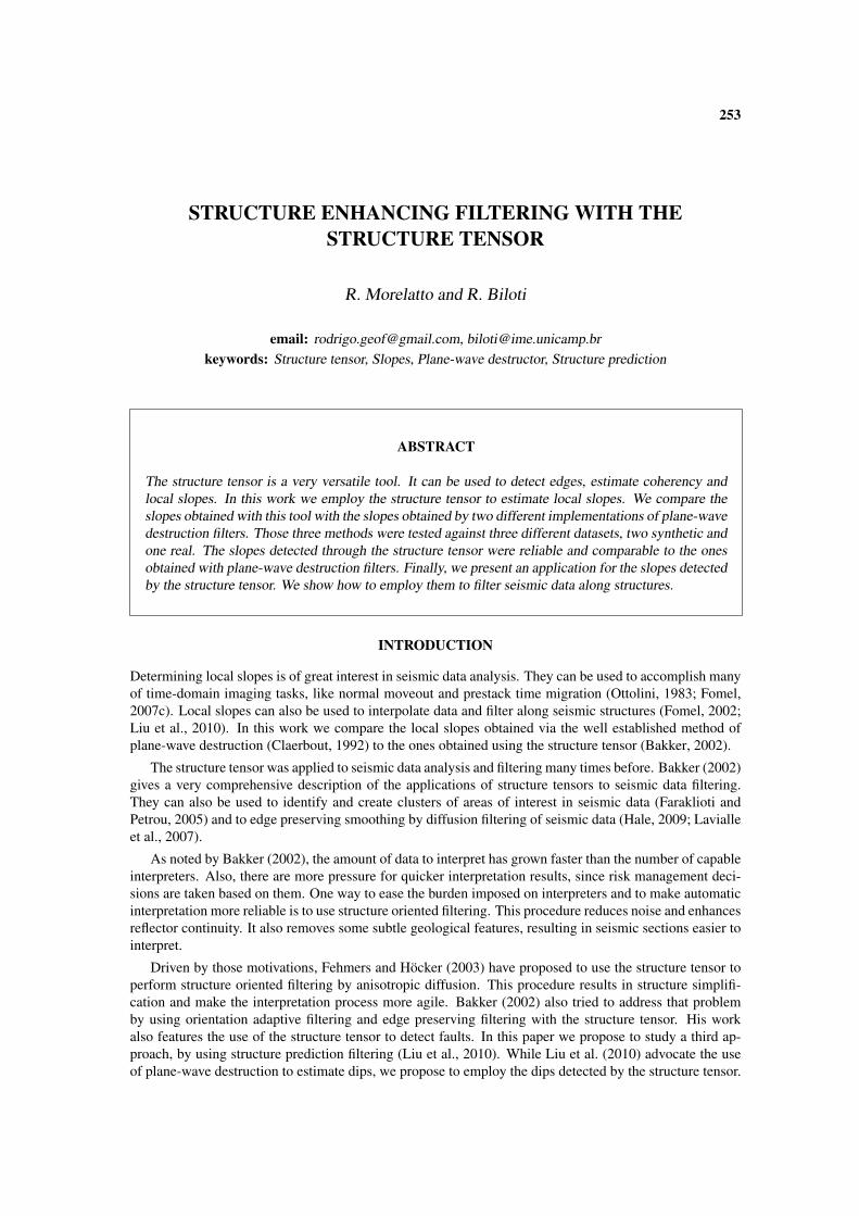
The second set is a synthetic sedimentary model (Figure 4(a)). Proposed by Claerbout (1992), thisdataset is composed by 200×200 pixels, spaced by 8 m in the x axis and 4 ms in the t axis. Finally, the lastdataset (Figure 5(a)) is a time-migrated seismic image from a historic Gulf of Mexico dataset (Claerboutand Green, 2010). It’s composed by 250×876 pixels with the time sampling of 4 ms, and spacing betweenconsidered as unitary. The data was also filtered with an AGC filter using triangular weights and half-second window.

Before we obtain the slopes or other seismic attributes, we want to take a look at the tensor eigenvalues,given by equations (15) and (16). The eigenvalues are shown in figures 3(b) and 3(c) for the dipping planesdataset, figures 4(b) and 4(b) for the synthetic sedimentary model and figures 5(b) and 5(b) for the fielddata.

It is important to note that the values of λ2 for the last dataset seem to be higher at the normal faultspresent in data (Figure 5(c)). This behavior is not totally unexpected. If we recall the relations betweenλ1 and λ2, listed on Table 1, we can see that the faults may be considered corner points. This behavior forthe eigenvalues matches with common geological interpretation intuition, considering that the faults areregistered as event terminations.

(a) Dipping planes model.

(b) First eigenvalue.

(c) Second eigenvalue.

Figure 3: Eigenvalues for the dipping planesmodel in (a), composed of 200 × 200 samplesand five plane events. In (b) we have the eigen-values for that model, computed with equa-tion (15) and an 5 × 5 integration scale sizewith Gaussian like weights (17). Finally, in (c)we have the second eigenvalue, computed withequation (16) and the same window and weightsof (b).

Let e1 and e2 be eigenvectors corresponding to eigenvalues λ1 and λ2. As discussed before, the eigen-vector e2 is parallel to the seismic image structures. We can estimate the data local slope by using the


(a) Synthetic sedimentary model.



Figure 4: Eigenvalues for the synthetic sedi-mentary model in (a), composed of 200 × 200samples. In (b) we have the eigenvalues forthat model, computed with equation (15) andan 5 × 5 integration scale size with Gaussianlike weights (17). Finally, in (c) we have thesecond eigenvalue, computed with equation (16)and the same window and weights of (b).

inclination of e2 as

σ =λ2 −

⟨P 2x

⟩〈PxPt〉

. (18)

Since e1 is orthogonal to e2, we can also use it to estimate the local slope as

σ = − 〈PxPt〉λ1 − 〈P 2

x 〉. (19)

COMPARISON OF LOCAL SLOPES ESTIMATION METHODS

In order to judge the quality of the slopes obtained with the structure tensor we need to compare its resultswith other methods. We choose to compare it with the well-known method of plane-wave destruction(Claerbout, 1992). We compare two different implementations of that method. For the sake of brevity welet to the reader to pursue further explanation of both methods.

The first formulation was suggested by Fomel (2002), it treats the plane-wave filter as a time-distance(t-x) prediction-error filter. Let the local plane wave equation be given by

Px + σ Pt = 0, (20)

where P is the wave field. Assuming that the slope σ(x, t) varies in both directions, one can design alocal filter to propagate a trace to its neighbors. The filters are obtained with the help of an implicit finite-difference scheme for the local plane-wave equation.

Let the seismic section s = [s1 s2 s3 . . . sn]T be a collection of traces. The plane-wave destructionoperation can be defined in a linear operator notation as

r = D(σ)s , (21)


(a) Time-migrated field data.



Figure 5: Eigenvalues for the time-migratedfield data in (a), composed of 250 × 876 sam-ples. In (b) we have the eigenvalues for thatmodel, computed with equation (15) and an5 × 5 integration scale size with Gaussian likeweights (17). Finally, in (c) we have the sec-ond eigenvalue, computed with equation (16)and the same window and weights of (b).

where r is the destruction residual. D is the non-stationary plane-wave destruction operator. The previousequation leads to the system of equations

r1

r2

r3

...rN

=

I 0 0 · · · 0

−P1,2(σ1) I 0 · · · 0

0 −P2,3(σ2) I. . . 0

... · · · · · · · · ·...

0 0 · · · −PN−1,N (σN−1) I

s1

s2

s3

...sN

, (22)

where I stands for the identity operator, σi is local dip pattern, and Pi,j(σi) is an operator for predictionof trace j from trace i. The destruction residual is minimized using regularized least-squares optimization.This is the essence of the method proposed by Fomel (2010) to estimate σ.

The second method, proposed by Schleicher et al. (2009), is based on a windowed fit of the data tothe plane-wave equation using total least squares. The data derivatives are estimated for x and t, then theslope is obtained by fitting these derivatives to the plane wave equation inside a small window. The slopeis considered to be constant in each window. In order to estimate the slope one just needs to use

σ = −sign

∑(i,j)∈W

Px(xi, tj)Pt(xi, tj)

√√√√√√

∑(i,j)∈W

P 2x (xi, tj)∑

(i,j)∈WP 2t (xi, tj)

, (23)

where i and j are the indices inside W window and σ is the estimated slope. The equation (23) is the totalleast-squares fit of equation (20) to the data derivatives inside the moving window W . The derivatives used


are the same ones used for the structure tensor, both estimated using a smooth first derivative program ofthe Madagascar package (sfsmoothder) with standard parameters. On the test data, the window W is 5× 5samples in every test case. To improve the results for the local plane wave destruction implementation, itsderivatives had been smoothed with the same Gaussian kernel of the structure tensor i.e. 5 × 5 samplessuport and (17) weights.

(a) Structure tensor local slopes. (b) Local plane-wave destructor local slopes.

(c) Global plane-wave destructor local slopes.

Figure 6: Comparison between local slopes ob-tained with the structure tensor (a), local (b) andglobal (c) plane-wave destructor implementa-tions for the dipping planes model (Figure 3(a)).

In Figure 6 we compare the dips obtained by the three methods above for the dipping planes dataset. Wecan easily note that the smoother estimate is the one obtained by the global minimization method (Figure6(c)). This lies on the fact that this method uses a global minimization with regularization, which forcessmooth variations of dips estimations.

As seen in figures 6(b) and 7(b), the estimation based on the local implementation of the plane-wavedestructor is almost visually equivalent to the structure tensor. This fact may be expected for simple testcases, since both methods have common characteristics as local support.

We also need to be careful on choosing an appropriated window size, because this method considerthe events on each window as a single plane wave propagation. This may be a problem, if we want eachpixel to represent just the slope of the event passing thought the center of the window. As seen in Figure8(b), there are horizontal outlier values lines accross the figure. Tweaking the window size may solve thisproblem. Also, comparing figures 8(a) and 8(b), the structure tensor slope estimation seem to be a bit moresmooth, without the afore mentioned outlier values lines.

One of the main advantages of the structure tensor is that each pixel corresponds mainly to the slopeon the center of the window. This is due to the tensor construction, specially if we use a Gaussian likewindow. The structure tensor slope estimation was comparable to the global plane-wave destructor, as seenin Figure 6(a). With the advantage of being faster to run and simpler to implement.



(c) Global plane-wave destructor local slopes. (d) Smoothed slopes estimated using the structure tensor.

Figure 7: Comparison between local slopes for the synthetic sedimentary model (Figure 4(a)). The slopesobtained with the structure tensor are shown in (a). A second version (d) of those slopes was obtained bysmoothing (a) three times with a 15× 15 triangular window. Finally, the local slopes for the same datasetusing the local (b) and global (c) plane-wave destructor implementations.

The slopes were estimated using the first eigenvalue and the equation (18). This eigenvalue was ob-tained using equation (15). If calculated without proper care, λ2 may suffer from loss of significance. Bycalculating it using equation (16) the dips obtained with equation (19) are equivalent to the ones obtainedwith λ1 and equation (18).

By comparing figures 7(a) and 7(c), it’s possible to conclude that the structure tensor slopes are a littleless smooth than the slopes of the global implementation of plane-wave destruction. The slopes obtainedwith the structure tensor are based on sums over data derivatives. This derivatives can be a little noisy,even after applying smoothing procedures. A possible workaround is to further smooth the data beforedifferentiation, taking care to not blur the reflector’s edges too much.

Smoother slopes can be obtained by changing the local and integration scales. Greater local scalemake the structure tensor ignore smaller details. The integration scale should reflect the characteristic sizeof the texture of interest (Weickert, 1999), in this case it should reflect the seismic events size. Instead ofincreasing the scale’s size, we choose to smooth the slopes obtained three times with a triangular smoothingwindow of 15× 15 samples, obtaining the slopes showed in Figure 7(d). The results of this procedure arealmost visually identical to the results of the global plane wave destruction, as seen by comparing figures7(d) and 7(c). This fact suggests that both estimations are almost equivalent, if proper smoothing is applied.



(c) Global plane-wave destructor local slopes. (d) Smoothed slopes estimated using the structure tensor.

Figure 8: Comparison between local slopes for the time-migrated field data (Figure 5(a)). The slopesobtained with the structure tensor are shown in (a). A second version (d) of those slopes was obtained bysmoothing (a) three times with a 15× 15 triangular window. Finally, the local slopes for the same datasetusing the local (b) and global (c) plane-wave destructor implementations.

STRUCTURE PREDICTION FILTERING

There are many ways to accomplish structure-enhancing filtering of a seismic image, like diffusion filteringof seismic data (Lavialle et al., 2007) or steering Gaussian elongated windows along local slope patterns(Haglund, 1991). For performance testing purposes, we choose to filter along the structures using plane-wave prediction (Liu et al., 2010). The filtering scheme is shown in Figure 9.

A trace can be predicted by shifting it according to the local seismic event slopes. Consider the pre-diction operator Pi,j(σi) as an operator for prediction of trace j from trace i, according to the local slopepattern σi (see e.g. Fomel (2002) and Fomel (2010) for further details). It’s possible to predict a trace froma distant neighbor by simple recursion. So, predicting trace k from trace 1 is simply

P1,k = Pk−1,k · · · P2,3 P1,2. (24)

In this work we propose the use of the structure prediction with the dips estimated by the structuretensor, instead of using the ones estimated with plane-wave destruction. After estimating the slopes, wepredict a trace from its neighbors and stack the predicted traces with the original one. In that way weaccomplish the structure filtering (Liu et al., 2010).

We tested this filtering method with two datasets, the synthetic sedimentary dataset (Figure 4(a)), andthe Gulf of Mexico dataset (Figure 5(a)). We used the smoothed slopes estimated with the structure tensor,


Local slope estimation Predict traces from shifted neighbors of the central trace

Stack

Figure 9: Prediction filtering scheme for the tracein blue. After estimate the local slopes for allpoints in data, the original trace can be predictedby shifting the neighbouring traces following thelocal slopes. In this figure, only the neighboursin the immediate vicinity are used. Distant neigh-bours can also be used by recursion. After the pre-diction step, all predicted traces are stacked withthe original ones, accomplishing structure filter-ing.

showed in figures 7(d) and 8(d), to predict each trace from its seven nearest neighbors. At this point it ispossible to accomplish structure filtering by simply stacking the predicted and original traces. By doing so,we have the filtered data showed in figures 10(a) and 10(c).

(a) Filtered synthetic data by simply stacking the original andpredicted traces.

(b) Difference between the original data (Figure 4(a)) and thefiltered data (a).

(c) Filtered field data by simply stacking the original and pre-dicted traces.

(d) Difference between the original data (Figure 5(a)) and thefiltered data (c).

Figure 10: Structure prediction filtering for the synthetic sedimentary and field datasets. First, each tracewas predicted from its seven nearest neighbours. Then, all fourteen predicted traces and the original onesare stacked, generating the sections in (a) and (c) for the synthetic and real datasets. The difference betweenand the original data is shown in (b) and (d) for the synthetic and real datasets.

First, let us discuss the results concerning the synthetic dataset. The noise was clearly attenuated, but


the fault and the interface between the folded layers and the plane layers was smeared. This effect isvery clear when we calculate the difference between the original and filtered data (Figure 10(b)). Thereare also some small data loss at the ends of the folded layers. This may be due to the increased error intrace prediction, since steeper slopes may have bigger errors associated. This effect is also enhanced if thepredicted traces are too far away from the original trace.

As seen in Figure 10(d), we can’t see much of that effect on the real dataset. This may be due to thesmall slope of the seismic reflectors. What is very clear is the loss of information at the reflectors ends,blurring the normal faults present in data. Nevertheless, the results were satisfactory and the data coherenceand reflectors continuity was improved, as shown in Figure 10(c). Again, this may be due to the data beingcompose mainly of planar like reflectors, which suits structure prediction filtering better.

SIMILARITY FILTERING WITH GAUSSIAN WEIGHTS

To prevent the blurring of data near faults and stratigraphic interfaces, we decided to improve the structurefiltering by using similarity based filter weights for the stacking step (Liu et al., 2010). The basic filteringscheme is explained in Figure 11. For the similarity weights, we use the definition of local similarityproposed by Fomel (2007a). This version of local similarity is defined using shaping regularization andlocal correlation. Shaping regularization expands Tikhonov’s regularization using a smoothing operator asthe regularization operator (Fomel, 2007b). This formulation makes the similarity vary smoothly, beingclose to one when the two traces compared are locally similar and approaching zero when they differ.

Local slope estimation Predict trace from its neighbours

Stacking with weights

Local similarity with the original trace

Figure 11: Local similarity enhanced prediction filtering scheme for the trace in blue. After estimate thelocal slopes for all points in data, the original trace can be predicted by shifting the neighbouring tracesfollowing the local slopes. In this figure, only the neighbours in the immediate vicinity are used. Distantneighbours can also be used by recursion. After the prediction step, local similarity between each predictedtrace and the original one is calculated. This similarity is used as stacking weights when all predicted tracesare stacked with the original one. This procedure results in local similarity enhanced structure filtering.

To further improve the data staking we employed a Gaussian taper. This results lower weights instacking for traces predicted from traces far from the original one, which diminishes some prediction errorsin the stacking (Liu et al., 2010). We multiply each trace by

wk = exp

(−k

2

ζ2

), (25)

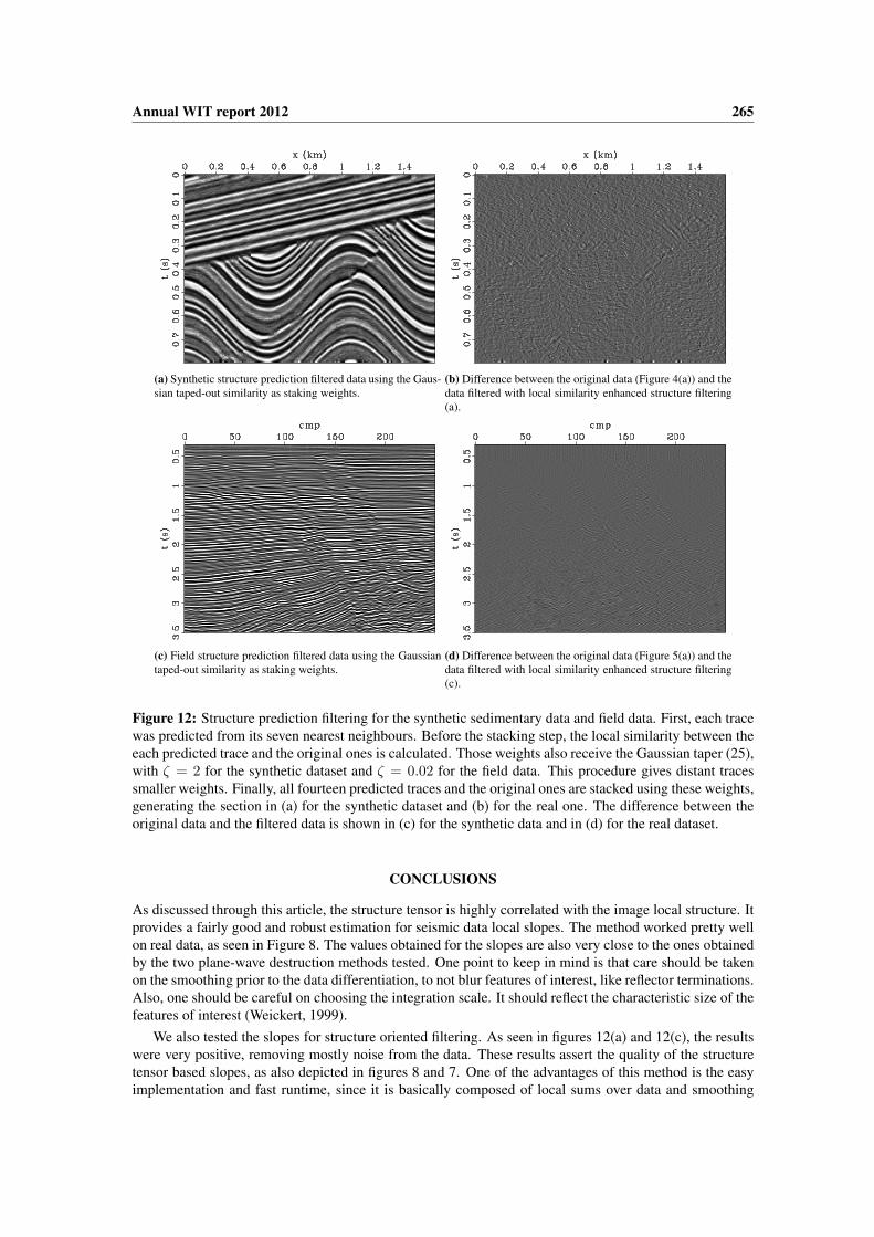
where wk is the Gaussian weight function, k is the index offset between the original and the predictedtraces, i.e. for the original trace k = 0, for a trace predicted using an immediate neighbour k = 1. Theparameter ζ alters the shape of the Gaussian. This approach is analogous to bilateral filtering (Tomasi andManduchi, 1998), with the advantage of smooth variation of the similarity weights. Finally, the filteringusing similarity stacking weights and ζ = 2 is showed in Figure 12(a) for the synthetic data. In Figure12(c), the same procedure was applied for the field data using ζ = 0.02. We can see that the noise wasattenuated, also there are very little smearing of the faults and other interfaces. This fact is further confirmedby the difference between the original data and the filtered data (figures 12(b) and 12(d)).


(a) Synthetic structure prediction filtered data using the Gaus-sian taped-out similarity as staking weights.

(b) Difference between the original data (Figure 4(a)) and thedata filtered with local similarity enhanced structure filtering(a).

(c) Field structure prediction filtered data using the Gaussiantaped-out similarity as staking weights.

(d) Difference between the original data (Figure 5(a)) and thedata filtered with local similarity enhanced structure filtering(c).

Figure 12: Structure prediction filtering for the synthetic sedimentary data and field data. First, each tracewas predicted from its seven nearest neighbours. Before the stacking step, the local similarity between theeach predicted trace and the original ones is calculated. Those weights also receive the Gaussian taper (25),with ζ = 2 for the synthetic dataset and ζ = 0.02 for the field data. This procedure gives distant tracessmaller weights. Finally, all fourteen predicted traces and the original ones are stacked using these weights,generating the section in (a) for the synthetic dataset and (b) for the real one. The difference between theoriginal data and the filtered data is shown in (c) for the synthetic data and in (d) for the real dataset.

CONCLUSIONS

As discussed through this article, the structure tensor is highly correlated with the image local structure. Itprovides a fairly good and robust estimation for seismic data local slopes. The method worked pretty wellon real data, as seen in Figure 8. The values obtained for the slopes are also very close to the ones obtainedby the two plane-wave destruction methods tested. One point to keep in mind is that care should be takenon the smoothing prior to the data differentiation, to not blur features of interest, like reflector terminations.Also, one should be careful on choosing the integration scale. It should reflect the characteristic size of thefeatures of interest (Weickert, 1999).

We also tested the slopes for structure oriented filtering. As seen in figures 12(a) and 12(c), the resultswere very positive, removing mostly noise from the data. These results assert the quality of the structuretensor based slopes, as also depicted in figures 8 and 7. One of the advantages of this method is the easyimplementation and fast runtime, since it is basically composed of local sums over data and smoothing


procedures. Those filtering results where further improved by the use of similarity weights (Figure 12)resulting in edge preserving structure oriented filtering. In the near future we intend to further test thestructure tensor filtering capabilities. We intend to use different types of adaptive filters and compare thoseresults with the results discussed above.

ACKNOWLEDGMENTS

This work was supported by the Instituto Nacional de Ciência e Tecnologia – Geofísica do Petróleo (INCT-GP), Brazil, and the sponsors of the WIT Consortium.

REFERENCES

Bakker, P. (2002). Image structure analysis for seismic interpretation. Ph.D. thesis, Delft University ofTechnology, Delft, Netherlands.

Claerbout, J. (1992). Earth soundings analysis: Processing versus inversion, volume 6. Blackwell Scien-tific Publications.

Claerbout, J. and Green, I. (2010). Basic earth imaging. Stanford University.

Faraklioti, M. and Petrou, M. (2005). The use of structure tensors in the analysis of seismic data. InIske, A. and Randen, T., editors, Mathematical Methods and Modelling in Hydrocarbon Explorationand Production, volume 7 of Mathematics in Industry, pages 47–88. Springer Berlin Heidelberg.

Fehmers, G. and Höcker, C. (2003). Fast structural interpretation with structure-oriented filtering. Geo-physics, 68(4):1286–1293.

Fomel, S. (2002). Applications of plane-wave destruction filters. Geophysics, 67(6):1946–1960.

Fomel, S. (2007a). Local seismic attributes. Geophysics, 72:A29–A33.

Fomel, S. (2007b). Shaping regularization in geophysical-estimation problems. Geophysics, 72(2):R29–R36.

Fomel, S. (2007c). Velocity-independent time-domain seismic imaging using local event slopes. Geo-physics, 72(3):S139–S147.

Fomel, S. (2010). Predictive painting of 3d seismic volumes. Geophysics, 75(4):A25–A30.

Haglund, L. (1991). Adaptive multidimensional filtering. Ph.D. thesis, Linköping University, Linköping,Sweden.

Hale, D. (2009). Structure-oriented smoothing and semblance. CWP Report, 635.

Lavialle, O., Pop, S., Germain, C., Donias, M., Guillon, S., Keskes, N., and Berthoumieu, Y. (2007).Seismic fault preserving diffusion. Journal of applied geophysics, 61(2):132–141.

Liu, Y., Fomel, S., and Liu, G. (2010). Nonlinear structure-enhancing filtering using plane-wave prediction.Geophysical Prospecting, 58(3):415–427.

Ottolini, R. (1983). Velocity independent seismic imaging. SEP-37: Stanford Exploration Project, 59:68.

Schleicher, J., Costa, J., Santos, L., Novais, A., and Tygel, M. (2009). On the estimation of local slopes.Geophysics, 74(4):P25–P33.

Tomasi, C. and Manduchi, R. (1998). Bilateral filtering for gray and color images. In Computer Vision,1998. Sixth International Conference on, pages 839–846. IEEE.

Weickert, J. (1999). Coherence-enhancing diffusion filtering. International Journal of Computer Vision,31(2):111–127.

Documents

STRUCTURE ENHANCING FILTERING WITH THE STRUCTURE TENSOR