Structure creation of P3HT in solution - Pure - … Isabelle Structure Creation of P3HT in Solution The work described in this thesis forms part of the research program of the Dutch

Structure creation of P3HT in solution

Monnaie, I.

Published: 01/01/2015

Document VersionPublisher’s PDF, also known as Version of Record (includes final page, issue and volume numbers)

Please check the document version of this publication:

• A submitted manuscript is the author's version of the article upon submission and before peer-review. There can be important differencesbetween the submitted version and the official published version of record. People interested in the research are advised to contact theauthor for the final version of the publication, or visit the DOI to the publisher's website.• The final author version and the galley proof are versions of the publication after peer review.• The final published version features the final layout of the paper including the volume, issue and page numbers.

Link to publication

Citation for published version (APA):Monnaie, I. (2015). Structure creation of P3HT in solution Eindhoven: Technische Universiteit Eindhoven

General rightsCopyright and moral rights for the publications made accessible in the public portal are retained by the authors and/or other copyright ownersand it is a condition of accessing publications that users recognise and abide by the legal requirements associated with these rights.

• Users may download and print one copy of any publication from the public portal for the purpose of private study or research. • You may not further distribute the material or use it for any profit-making activity or commercial gain • You may freely distribute the URL identifying the publication in the public portal ?

Take down policyIf you believe that this document breaches copyright please contact us providing details, and we will remove access to the work immediatelyand investigate your claim.

Download date: 25. Jun. 2018

https://research.tue.nl/en/publications/structure-creation-of-p3ht-in-solution(decf09a5-a757-407c-9152-fa8614018011).html

Structure Creation of P3HT

in Solution

PROEFSCHRIFT

ter verkrijging van de graad van doctor aan de Technische Universiteit

Eindhoven, op gezag van de rector magnificus prof.dr.ir. C.J. van Duijn,

voor een commissie aangewezen door het College voor Promoties, in het

openbaar te verdedigen op maandag 23 februari 2015 om 14:00 uur

door

Isabelle Monnaie

geboren te Antwerpen, België

Dit proefschrift is goedgekeurd door de promotoren en de samenstelling

van de promotiecommissie is als volgt:

voorzitter: prof.dr.ir. J.C. Schouten

1e promotor: prof.dr. E.L.F. Nies

2e promotor: prof.dr. G. de With

leden: prof.dr. W.J. Briels (Universiteit Twente) dr. B. Goderis (Katholieke Universiteit Leuven)

prof.dr.ir. R.A.J. Janssen

prof.dr. D.J. Broer

adviseur: dr. S. Veenstra (Energieonderzoek Centrum Nederland)

Monnaie, Isabelle

Structure Creation of P3HT in Solution

The work described in this thesis forms part of the research program of the

Dutch Polymer Institute (DPI), Technology Area Functional Polymer Systems, DPI project #682.

A catalogue record is available from the Eindhoven University of

Technology Library.

ISBN: 978-90-386-3783-9

Cover design: Marco Hendrix and Isabelle Monnaie

Printed by: Gildeprint - www.gildeprint.nl

Contents

Summary ix

CHAPTER 1. Introduction 1

1.1 The Energy Challenge 2

1.2 Organic Photovoltaic Cells 4

1.3 Working Principle of Bulk Heterojunction SCs 6

1.4 Evolution of Organic Solar Cell Materials 8

1.4.1 Donors 9

1.4.2 Acceptors 10

1.5 Properties Influencing the Morphology in P3HT/PCBM 10

1.5.1 P3HT 11

1.5.2 PCBM 13

1.5.3 Influence of Processing Conditions on the Blend Morphology 13

1.6 Objective and Outline of this Thesis 15

References 17

CHAPTER 2. The Influence of Regioregularity on the

Determination of Fundamental Chain Parameters of P3HT by

SANS 23

2.1 Introduction 24

2.2 Experimental Section 25

2.2.1 Materials 25

2.2.2 Conventional Characterization Methods 25

2.2.3 SANS Setup and Data Treatment 25

2.2.4 Sample Preparation for SANS and UV-vis 26

2.3 Results and Discussion 26

2.3.1 Synthesis 26

2.3.1.1 Synthesis of Poly(3-hexylthiophene)s 26

2.3.1.2 Mechanistic Implications 28

2.3.2 SANS Results 29

2.3.2.1 Scattering due to Concentration Fluctuations and Form Factor 29

2.3.2.2 Limiting Low q Analysis 32

2.3.2.3 Determination of Persistence Length via the Holtzer

Representation 33

2.3.2.4 Relationship between Mw and ⟨Rg2⟩z 35

2.4 Conclusions 37

References 39

APPENDIX to Chapter 2 43

A2.1 GRIM Mechanism 44

A2.2 1H-NMR Spectra of P3HT Samples 44

A2.3 Calculation of the Volume Fractions 46

A2.4 Calculation of the Contrast Factor per Unit Volume 46

A2.5 Overlap of Scattering Patterns When Taking Into Account Polymer Volume

Fraction 47

A2.6 Limiting Low q Analysis 47

A2.7 Analysis of the Scattering Pattern by Use of Models 48

A2.8 Parameter Estimation Procedure and Fitting Algorithm 50

A2.9 Fitting Parameters 50

A2.10 Comparison Between Model Analysis and LLq 53

A2.11 Persistence Length versus Regioregularity From the Model Fitted Patterns 54

References 56

CHAPTER 3. Conformational Properties of Excluded Volume

Semi-Flexible Polymers: Simulation Approach 57

3.1 Introduction 58

3.2 Theoretical Background 59

3.2.1 Freely Jointed Chain (FJC) Model 59

3.2.2 Semi-Flexible Chain (SFC) Model 60

3.2.3 Semi-Flexible Hard Sphere Chain (SFHSC) Model 61

3.2.4 Models for the Single Chain Form Factor 62

3.3 Simulation Methods 63


3.4.1 Method Validation for Ideal Chains 64

3.4.2 Semi-Flexible Chains (SFC) 66

3.4.3 Semi-Flexible Hard Sphere Chains (SFHSC): Excluded Volume and

Stiffness 71

3.4.4 P3HT Single Chain Properties by Simulation 76

3.5 Conclusions 82

References 84

CHAPTER 4. The Phase Behavior of P3HT: Influence of

Regioregularity and Molar Mass 85

4.1 Introduction 86


4.2.1 Materials 87

4.2.2 Solution Preparation 88

4.2.3 Differential Scanning Calorimetry 88


4.3.1 Thermal Analysis of Crystallization and Melting of P3HT 89

4.3.1.1 Molar Mass Dependence of Tm 91

4.3.1.2 Regioregularity Dependence of the Thermal Behavior 93

4.3.1.3 Combining Molar Mass and Regioregularity Dependence 95

4.3.2 The Phase Behavior of P3HT in Solution 96

4.3.2.1 General Phase Transition Observations in Solution 98

4.3.2.2 Phase Behavior at Low P3HT Concentrations 98

4.3.2.3 Phase Diagrams of P3HT/Toluene and P3HT/ODCB 100

4.4 Conclusions 103

References 105

CHAPTER 5. Time and Temperature Dependence of

P3HT/Toluene Gel Formation 107

5.1 Introduction 108


5.2.1 Materials and Solution Preparation 109

5.2.2 Methods 109

5.2.2.1 Differential Scanning Calorimetry 109

5.2.2.2 In-House Rheology 109

5.2.2.3 In-Line Rheology - SANS 110

5.2.2.4 Cryo-Transmission Electron Microscopy (Cryo-TEM) 111

5.2.3 General Time-Temperature Profile 111


5.3.1 Time Dependent Gelation at Room Temperature 112

5.3.2 Influence of Mild Changes in Thermal History 114

5.3.3 Rheological Behavior for P3HT Gels formed at Tiso = 5 °C 115

5.3.4 Thermal Analysis of the Gel Samples 117

5.3.5 In-Line Rheology – SANS: Analysis of the Network Structure 120

5.3.5.1 In-line Rheology 121

5.3.5.2 Small-Angle Neutron Scattering 122

5.3.5.3 Combining SANS, Rheology Observations and Thermal Analysis 128

5.3.6 The Proposed P3HT Network Morphology and its Temperature

Dependence 130

5.4 Conclusions 133

References 134

APPENDIX to Chapter 5 137

A5.1 In-Line Rheology - SANS: Temperature Control 137

Epilogue 139

Acknowledgements 145

Curriculum Vitae 149

ix

SUMMARY

Structure Creation of P3HT in Solution

The global energy demand will continue to increase in the coming decades. The

drawbacks of the main energy sources which are currently used (fossil fuels,

nuclear fission), are part of the incentive to further develop technologies capable of

using renewable energy sources, such as solar energy. Solar cells convert solar

photons into electricity and the amount of electricity that can be produced is

strongly dependent on the efficiency of the photovoltaic device and the available

surface area. Organic solar cells are a promising low-cost alternative to silicon-

based solar cells, as they can be fabricated by inkjet or roll-to-roll printing of

organic materials. However, they are characterized by lower power conversion

efficiencies and limited life times.

In polymer/fullerene photovoltaic cells, the photoactive layer of consists of a

donor (D) material (polymer, here poly(3-hexylthiophene), P3HT) and an acceptor

(A) material (fullerene, e.g., PCBM). The morphological requirements are sufficient

layer thickness (photon absorption, exciton generation), large D-A interface area

accessible within the exciton diffusion limit (free charge generation) and co-

continuous pathways to the electrodes (charge transport).

P3HT/PCBM solar cells have been profiled in literature as a model system and

the photoactive layer of these devices is generally prepared by casting an ink, a

homogeneous solution of both D and A materials in organic solvent, on a substrate

by spin coating. During deposition and evaporation, the photoactive layer

morphology is formed by crystallization of the components (P3HT forms semi-

crystalline nanowire structures) and this “kinetically frozen” morphology can be

further optimized by post-production thermal annealing. Therefore, the final

photoactive layer morphology is strongly dependent on processing conditions and

external factors. The development of an ink, which contains already the desired

P3HT nanostructures or their precursors, can provide increased control over the

Summary

x

formed morphology since structure formation can then be decoupled from the

deposition step.

In the research described in this thesis, we have investigated the intrinsic

conformational properties of P3HT, as function of molar mass and regioregularity

(RR), as well as the structure formation of P3HT in solution (toluene), with respect

to time and temperature.

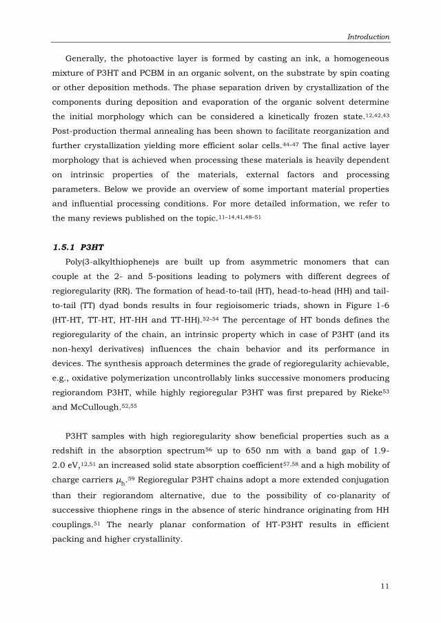
Chapter 2 starts with the experimental study of the fundamental single chain

properties of different P3HT polymers by small-angle neutron scattering (SANS). We

use limiting low q analysis to obtain estimates for molar mass (Mw) and radius of

gyration (⟨Rg2⟩1 2⁄ ). We show that conventional characterization by SEC significantly

overestimates the molar mass of P3HT and observe an effective scaling relationship

between chain length and ⟨Rg2⟩1 2⁄ where the exponent ν = 0.66 is determined both

by stiffness and excluded volume interactions in the chain. A measure for the

chain stiffness of the polymer chain, persistence length (Lp), was determined by the

Holtzer method. The persistence length scales linearly with polymer regioregularity

(studied for 89% ≤ RR ≤ 99%, with 38 Å ≤ Lp ≤ 51 Å).

These estimates are obtained via model-independent analyses and can,

therefore, be considered the best available experimental values for these polymers.

In the Appendix to Chapter 2, we show that widely employed form factors

developed for semi-flexible polymers, do not accurately fit the SANS patterns of

P3HT.

To provide better understanding of the influence of chain stiffness and excluded

volume interactions on the chain conformational properties, we describe the

computational study of coarse-grained semi-flexible polymer chains (without and

with excluded volume interactions) in Chapter 3. Configurational-bias Monte Carlo

(cbMC) simulations of chains with different length and bending stiffness are

analyzed for the average squared end-to-end distance ⟨R2⟩ and radius of gyration

⟨Rg2⟩, and persistence length Lp. The form factor P(q) is calculated and the Holtzer

method, to experimentally determine Lp, is validated with proportionality constant

C = 3.6 ± 0.2. The size of the chains shows a variety of intermediate scaling

exponents depending on chain length N and bending constant kb. Excluded volume

interactions, implemented as a hard sphere interaction potential, influence the size

and persistence of flexible polymer chains. With increasing stiffness, the excluded

Summary

xi

volume contribution diminishes gradually, with the decay being slower for longer

chains. At the rigid rod level, the excluded volume effect is absent and, therefore,

the Holtzer analysis remains unaffected.

Simulation of P3HT polymers as semi-flexible hard sphere chains (SFHSC) and

comparison with the experimental form factors (studied in Chapter 2), show that

excluded volume effects should be included when accurately describing these

polymers.

Chapter 4 describes the phase behavior of P3HT as investigated with differential

scanning calorimetry (DSC). We study the melting behavior of different P3HT

polymers (in powder form) and the influence of molar mass and regioregularity. For

short chains with low RR, the effect of regioregularity dominates the melting point

depression. For solutions of P3HT with toluene or ODCB, binary phase diagrams

are constructed and an additional reversible invariant thermal transition is

observed. At low concentrations, the melting point depression with respect to RR is

similar to the behavior observed for the powders. We have strong indications of a

different morphology of the P3HT dispersions in toluene versus ODCB.

Solutions of low-polymer content RR-P3HT in toluene undergo gelation when

stored at ambient temperatures. The network formation and its internal structure

are investigated in Chapter 5, by combining rheological measurements and SANS

and varying the isothermal aging temperature and time. Upon cooling the

homogeneous P3HT solution and crossing the sol-gel point, the network structure

grows rapidly and continues to evolve for isothermal aging times of up to 8 hours

at room temperature.

Cryo-TEM images of the gelled samples indicate an inhomogeneous

morphology, which we show consists of a P3HT-depleted matrix phase and P3HT-

enriched domains, the latter containing cross-link clusters. The elastic modulus of

the bimodal P3HT network is dominated by the internal structure of the P3HT-

enriched clusters, i.e., the cross-link domains.

CHAPTER 1

Introduction

The global energy problem and the drawbacks of current energy producing

technologies serve as motivation for research on organic solar cells. Basic working

principles, device architecture and standard solar cell characterization are

discussed, before highlighting two major routes leading to improved performance:

active layer morphology optimization and molecular design. More detailed

information on the properties of the model system P3HT/PCBM is given and

influential processing parameters are discussed. Finally, the objective of this thesis

is formulated, followed by the organization of the chapters.

Chapter 1

2

1.1 The Energy Challenge

Throughout history, people have become increasingly dependent on energy.

Western societies even demand a guaranteed and continuous supply of energy as it

is required in all aspects of daily life. In 2012 the global primary energy

consumption increased by 1.8%, less than the 10-year average of 2.6%, but still

estimated at approximately 524 EJ. This corresponds to an overall power of 17 TW.

China was the most consuming country with a share of 21.9%, comparable to the

regions North America (21.8%) and Europe as a whole (23.5%), placing Asia in the

energy consumption statistics with a share of 40.0% and a 4.7% growth since

2011. The continent of Africa also noted a +4.7% change during 2012, but this

developing region only makes up for 3.2% of the global primary energy

consumption, for now.1 In addition, the prospected growth of the human

population from 6.9 billion in 2011 to 9.3 billion in 2050 is believed to occur

mainly in less developed regions, while the population in more developed countries

will remain essentially unchanged (1.2 billion in 2011 to 1.3 billion in 2050).2 Both

phenomena combined will lead to a severely increased global demand for energy in

the coming decades.

Nowadays, the main sources of energy are fossil fuels (87%, of which 33% oil,

24% natural gas and 30% coal), nuclear fission (4.5%) and renewable energy

sources (8.5%).1 Both fossil fuels and nuclear fission technologies come with

serious drawbacks and (can) have a large impact on the environment. The limited

supply of fossil fuels makes this energy source destined to fall short in the future.

The geographic distribution of oil, natural gas and coal sources is restricted to

certain regions of the world, which results in political and economic imbalance.

Furthermore, the use of fossil fuels is inevitably linked to the production of

greenhouse gases and the issue of global warming, as 56.6% of the greenhouse

gases emitted by human activity originate from the consumption of fossil fuels.3

Nuclear fission of uranium, on the other hand, does not contribute to climate

change but creates large amounts of nuclear waste which need to be stored for

decades, if not centuries, awaiting the decay of the formed isotopes. The potential

danger of this technology has been confirmed by nuclear disasters, the most recent

in Fukushima, Japan in 2011 where an earthquake caused equipment failure

leading to nuclear meltdowns and the release of radioactive materials from the site.

Introduction

3

Renewable energy is considered a potential replacement for these traditional

energy sources as they are often also referred to as “clean” sources of energy with a

smaller ecological footprint. Some examples of renewable energy sources are

hydroelectric (78% of the total energy consumption from renewables),1 solar, wind,

geothermal and biomass. Disregarding hydroelectricity, renewable energy

consumption noted a 15.2% increase over 2012,1 illustrating the growing relevance

of these technologies. Scarcity of elements or materials is less of an issue in this

case, but while the combustion of biomass is still related to the production of

greenhouse gases impacting climate change, other renewable sources are

characterized by notable geographical limitations.

Solar energy, however, is distributed abundantly, albeit not evenly,3 over the

entire earth’s surface, allowing technologies which exploit this source to be used

without geographical restrictions. Approximately 1.2·105 TW of solar energy

continuously reaches the earth’s surface, of which an estimated maximum of

1.5·103 TW is available to be put to human use, significantly (almost 100 times)

higher than the present annual global consumption.3 As solar energy can be

transformed into both heat and electricity, further references to solar energy

technology are directed towards the conversion of solar energy into electricity by

use of photovoltaic devices or solar cells (SCs).

There are still a number of challenges to overcome before solar energy

technology can provide a large part of the energy demand. The amount of electricity

that can be produced from solar energy depends heavily on the efficiency of the

devices used and the available surface area. For silicon-based solar cells, averaging

at an efficiency of 15-20%, an area the size of at least 425·103 km2 (covering, e.g.,

85% of Spain) is required to meet the 2012 global energy consumption of 17 TW.4

The requirement for vast areas covered with solar panels makes the total

production cost an important consideration. Silicon-based solar cells are

characterized by a high cost per unit area due to the sensitivity of the fabrication

process to impurities, requiring large clean room facilities. Also, the limited

availability of silicon will make this raw material increasingly more expensive with

time.

Organic solar cells (OSC), fabricated by inkjet or roll-to-roll printing of organic

materials, can be a promising low-cost alternative. Challenges in different aspects

of this technology still hamper its commercial development, as they are

Chapter 1

4

characterized by lower power conversion efficiencies and shorter life times than

their inorganic substitutes.

1.2 Organic Photovoltaic Cells

In 1839, Becquerel first demonstrated the photovoltaic effect, by which photons

are converted into electricity.5 The first silicon solar cell was reported in 1954,6

while the presence of the photovoltaic effect in organic semiconductors was first

patented in 1979.7 Photovoltaic cells can be categorized according to the types of

materials used in the photoactive layer of the devices. Inorganic solar cells are

often based on silicon and come in two varieties. Traditional silicon solar cells have

a hundreds of micrometer thick layer of high-purity defect-free silicon single

crystals. They hold the majority of the market share of currently available

photovoltaic technology with a reported record performance of 25.0%.8 Thin film

devices have an active layer in the range of only few hundred nanometers thick and

can be made from nanocrystalline (10.1%) or amorphous silicon (10.1%) or other

materials, e.g., copper indium gallium diselenide (CIGS, 19.6%) or cadmium

telluride (CdTe, 18.3%).8

Organic solar cells typically group photovoltaic technologies that contain at

least one organic component in the photoactive layer. The most common categories

are: dye sensitized (Grätzel, 11.9%) solar cells,8 hybrid solar cells, which use

organic materials as matrix in which inorganic semiconducting nanoparticles are

embedded (3%)9 and all-organic technologies. The latter contain small molecule

solar cells,10 fabricated through vacuum deposition, and solution processed SCs.

Solution processed organic solar cells (10.7%)8 can be all polymer cells, small

molecule cells10 or polymer/fullerene cells,11–14 the latter being by far the more

developed and most promising technology, often referred to simply as organic solar

cells.

Figure 1-1 shows the organization of layer stacks that make up a conventional

OSC device. The transparent substrate (here glass) is coated with a transparent

electrode, in laboratory devices mostly indium tin oxide (ITO). A hole conductive

layer such as poly(3,4-ethylenedioxythiophene):poly(styrenesulfonate) (PEDOT:PSS)

is deposited on top to facilitate hole extraction. An electron collecting electrode,

often lithium fluoride/aluminum, is placed on top of the photoactive layer. The

difference in work function of the two electrodes creates the internal electric field

Introduction

5

responsible for the generated free charges to move in opposite directions to their

respective electrodes.

Figure 1-1. Device architecture of a typical organic solar cell.

A solar cell is characterized by the current that can flow as a voltage is applied

across the electrodes. From the measured current density-voltage (J-V) curve, a

number of characteristic properties can be determined (Figure 1-2). The open-

circuit voltage (Voc) is defined in the condition where the total current through the

illuminated cell is zero. The short-circuit current density (Jsc) is defined at zero

applied bias, as if the circuit was short-circuited. The maximum power point (MPP)

is the point where the product of J and V is maximal and the cell produces its

maximum power Pmax. The ratio of Pmax and Jsc∙Voc is defined as the fill factor (FF),

a measure of ideality (Equation 1.1). The power conversion efficiency (PCE, η) is

defined in relation to the maximum power point as the ratio of Pmax and Pin, the

power of the incoming light (Equation 1.2).

FF = Pmax

Jsc∙Voc =

Jmax∙Vmax

Jsc∙Voc (1.1)

η = Pmax

Pin =

FF∙Jsc∙Voc

Pin (1.2)

Standard testing conditions for solar cells set Pin = 100 mW cm-2 at illumination

by the AM1.5G reference solar spectrum (air mass 1.5 global).15 This spectrum

represents the light that reaches the earth’s surface with a solar zenith angle of

48.2° (locations at temperate latitudes) after traveling through 1.5 times the

thickness of the earth’s atmosphere on a clear sunny day. This spectrum is

Chapter 1

6

simulated in the measurement setup by a lamp and the appropriate filters.

Certified efficiencies are measured at institutes such as the National Renewable

Energy Laboratory (NREL) (USA) or the National Institute of Advanced Industrial

Science and Technology (AIST) (Japan).

Figure 1-2. Typical J-V characteristics of an organic solar cell in dark (dashed line) and under illumination (solid line).

1.3 Working Principle of Bulk Heterojunction SCs

The working principle of an organic photovoltaic cell (OPV) is illustrated in

Figure 1-3.16 The consecutive steps in the process of converting solar photons into

electricity are explained in detail, noting the requirements they impose on the

materials and device structure.

The photoactive layer of these cells is built up by an electron-donating (donor,

D) material and an electron-accepting (acceptor, A) material. In the majority of

material combinations, the donor is responsible for the absorption of photons,

therefore this point of view is presented in Figure 1-3. Upon absorption, a tightly

bound electron-hole pair (exciton) is created which is located on the donor material

(a). The amount of absorbed photons is directly related to two aspects posing a first

set of requirements. The overall photoactive layer thickness is an important factor

determining whether sufficient photons can be absorbed. Generally, dimensions of

100 nm are considered optimal, as can be checked by optical modeling. Also, the

absorption spectrum of the photoactive material should be well matched with the

solar emission spectrum.

Introduction

7

In contrast to inorganic materials, the exciton binding energy in organic semi-

conductor materials is several orders of magnitude larger (0.4-0.6 eV)17–19 due to

the low dielectric constant of this type of materials. Only after diffusing to a

heterojunction between donor and acceptor (b), the photogenerated exciton can be

split into free collectable charges (c). The diffusion length of this electron-hole pair

is limited to approximately 4-20 nm,20–22 the exciton diffusion length in common

conjugated polymers. Maximizing free charge generation, a heterojunction should

be present within these spatial restrictions from any point within the bulk of the

photoactive layer. At the donor-acceptor interface, the electron that was promoted

to the lowest-unoccupied molecular orbital (LUMO) of the donor by absorption of a

photon, transfers from the donor material to the lower energetic LUMO of the

acceptor, effectively splitting the exciton into a free hole on the donor and a free

electron on the acceptor (d). Provided there are co-continuous pathways of both

phases to the electrodes, the charges can be collected and a current can flow

through the cell (e, f).

Figure 1-3. Energy diagram showing stepwise the conversion of light into electricity in an organic donor-acceptor solar cell; (a) generation of an exciton by absorption of a photon, (b) diffusion of the exciton to the interface, (c) charge transfer, (d) charge generation, (e) charge transport and (f) charge collection at the electrodes.

Listed above, the morphological requirements for the active layer, which allow

efficient power conversion, are sufficient layer thickness, access to a D-A

heterojunction interface within the exciton diffusion limit and co-continuous

pathways of both materials to the electrodes. Maintaining a total layer thickness in

Chapter 1

8

the range of 100 nm, a bilayer morphology where donor and acceptor materials are

layer stacked vertically (Figure 1-4a), complies to two of these requirements but

falls short in converting a sufficient amount of the formed excitons into free

charges. The average distance an exciton needs to overcome to reach the donor-

acceptor interface is too large and recombination processes hamper the generation

of free charges. Reducing the overall photoactive layer thickness and thus the

average distance to the heterojunction, limits light absorption and will negatively

impact the efficiency (Figure 1-4b).

The bulk heterojunction morphology (BHJ) adds a large interface area

distributed throughout the bulk of the photoactive layer to the conditions already

met by the thick bilayer construction. Figure 1-4c shows schematically how in the

bulk heterojunction donor and acceptor are blended together with a phase

separation in the order of nanometers, while maintaining continuous pathways to

the electrodes for each of the two materials.23,24

Figure 1-4. Photoactive layer morphologies in donor (red) - acceptor (blue) organic solar

cells; (a) thick bilayer, (b) thin bilayer, (c) bulk heterojunction.

The large interface between donor and acceptor constitutes the risk of increased

bimolecular recombination probability as free electrons and holes are in close

vicinity of each other while traveling to their respective electrodes. This means that

the dimensions of phase separation should be tuned accordingly, as a trade-off

between exciton diffusion length and recombination probability.

1.4 Evolution of Organic Solar Cell Materials

A nanoscale morphology intermixing both donor and acceptor positively

influences the power conversion efficiency. Tuning the intrinsic properties of the

photoactive layer materials is another focal point in the improvement of these solar

Introduction

9

cells. Below, some historically important, model materials and state-of-the-art

materials are discussed.

1.4.1 Donors

The organic semiconducting polymers used in OPVs have evolved tremendously

in the past decades. The Nobel prize winning discovery at the end of the 1970s (by

Heeger, MacDiarmid and Shirakawa, Nobel Prize in Chemistry 2000)25 in which

doped polyacetylene (the prototype π-conjugated polymer) was shown to reach a

conductivity level similar to metals,26,27 marked the start of decades of intense

research. While polyacetylene is an insoluble material, it was recognized that

highly soluble conductive polymers were needed. The first generation of these new

materials included polyphenylenevinylenes (PPV) and polythiophenes (PT). The first

solution processed BHJ solar cell consisted of poly[2-methoxy-5-(2’-ethyl-

hexyloxy)-1,4-phenylenevinylene] (MEH-PPV) in a 1:4 ratio with acceptor PCBM

(see the section below).24 While the synthesis methods were optimized, improving

purity, molecular weight and batch-to-batch uniformity, the influence of processing

parameters became apparent when the use of chlorobenzene instead of toluene

almost tripled the PCE to 2.5% in poly[2-methoxy-5-(3’,7’-dimethyloctyloxy)-1,4-

phenylenevinylene] (MDMO-PPV)/ PCBM solar cells.28 A new synthesis route for

MDMO-PPV delivered high-molecular weight and low-defect level polymers,

showing the importance of controlling the polymer regularity, with efficiencies of

nearly 3%.29 The relatively large bandgap and low charge transport mobility moved

the interest from PPV-based polymers to poly(alkylthiophene)s, among which

poly(3-hexylthiophene) (P3HT) received most attention. Intense research devoted to

different aspects of synthesis and processing led relatively quickly to 5% efficient

P3HT/PCBM solar cells.30,31

Polyfluorenes32 and polycarbazoles33 were developed later as deep highest-

occupied molecular orbital (HOMO), high Voc materials. Still suffering from small

photocurrent and wide bandgap, the attention was shifted to lower bandgap

materials (lower than 1.8 eV). Bridged bithiophenes (cyclopentadithiophene-based

polymers), such as PCPDTBT and its silicon-bridged counterpart (Si-PCPDTBT) still

showed a low Voc.34

The first material class combining small bandgap with low HOMO is PTB-based,

where side chains with electron donating or electron withdrawing properties

allowed tuning of, respectively, the HOMO and LUMO levels of the polymer and

Chapter 1

10

efficiencies of 6% were reported.35,36 Figure 1-5 shows the chemical structures of

some of the discussed donor polymers.

Figure 1-5. Molecular structure of selected donor polymers.

1.4.2 Acceptors

The wide range of donor polymers stands in large contrast with the limited

amount of acceptor materials developed since the introduction of the bulk

heterojunction. Making well-performing polymeric acceptors was proven

challenging, therefore n-type small molecules are most often used, soluble

derivatives of the C60 and C70 fullerenes in particular. The first reported solution

processed BHJ solar cells were made with [6,6] phenyl-C61-butyric acid methyl

ester ([60]PCBM). At the time efficiencies around 1% were reached and this

acceptor is still today the most popular one for OPVs.23,24,37,38 Noteworthy also is

[6,6] phenyl-C71-butyric acid methyl ester ([70]PCBM) which shows a higher

absorption in the visible region due to lower symmetry.39

1.5 Properties Influencing the Morphology in P3HT/PCBM

Since the first encouraging P3HT/PCBM solar cell report in 2002,40 record

efficiencies for this material combination in the range of 5% have been

achieved.30,31 Furthermore, P3HT/PCBM has been labeled as a model system as

these active materials are by far the most studied in this field.41

Introduction

11

Generally, the photoactive layer is formed by casting an ink, a homogeneous

mixture of P3HT and PCBM in an organic solvent, on the substrate by spin coating

or other deposition methods. The phase separation driven by crystallization of the

components during deposition and evaporation of the organic solvent determine

the initial morphology which can be considered a kinetically frozen state.12,42,43

Post-production thermal annealing has been shown to facilitate reorganization and

further crystallization yielding more efficient solar cells.44–47 The final active layer

morphology that is achieved when processing these materials is heavily dependent

on intrinsic properties of the materials, external factors and processing

parameters. Below we provide an overview of some important material properties

and influential processing conditions. For more detailed information, we refer to

the many reviews published on the topic.11–14,41,48–51

1.5.1 P3HT

Poly(3-alkylthiophene)s are built up from asymmetric monomers that can

couple at the 2- and 5-positions leading to polymers with different degrees of

regioregularity (RR). The formation of head-to-tail (HT), head-to-head (HH) and tail-

to-tail (TT) dyad bonds results in four regioisomeric triads, shown in Figure 1-6

(HT-HT, TT-HT, HT-HH and TT-HH).52–54 The percentage of HT bonds defines the

regioregularity of the chain, an intrinsic property which in case of P3HT (and its

non-hexyl derivatives) influences the chain behavior and its performance in

devices. The synthesis approach determines the grade of regioregularity achievable,

e.g., oxidative polymerization uncontrollably links successive monomers producing

regiorandom P3HT, while highly regioregular P3HT was first prepared by Rieke53

and McCullough.52,55

P3HT samples with high regioregularity show beneficial properties such as a

redshift in the absorption spectrum56 up to 650 nm with a band gap of 1.9-

2.0 eV,12,51 an increased solid state absorption coefficient57,58 and a high mobility of

charge carriers μh.59 Regioregular P3HT chains adopt a more extended conjugation

than their regiorandom alternative, due to the possibility of co-planarity of

successive thiophene rings in the absence of steric hindrance originating from HH

couplings.51 The nearly planar conformation of HT-P3HT results in efficient

packing and higher crystallinity.

Chapter 1

12

Figure 1-6. Isomeric triads of 3-substituted polythiophenes.

Also the molar mass of the polymer can be controlled by the synthesis

procedure. Increasing the molecular weight affects the absorption properties of the

polymer. The solid state absorption maximum λmax is red-shifted by more than

100 nm as Mn is increased by a factor 10.60 Also the charge carrier mobility for

holes μh in P3HT increases with molecular weight.61,62 Although the polydispersity

(PDI) will influence, e.g., crystal packing, a clear influence on the performance

cannot be found.41,63

Highly regioregular polymer chains of P3HT (with large Mw) form semicrystalline

nanowires, where laterally stacked thiophene main chains are separated by the

alkyl side chains and in the length dimension the nanowire is built up by multiple

of these lamella via π- π interactions.54,55,59,64,65 These nanowires are formed upon

evaporation of the solvent as a film is cast from the ink by any deposition method.

The creation of these semi-crystalline ordered structures is crucial to reach good

performance (charge carrier mobility and beneficial dimensions for BHJ

morphology). Another approach grew P3HT nanofibers in solution by lowering the

sample temperature66–69 or by addition of poor solvent such as hexane.70,71

The gelation of P3HT in organic solvents such as toluene and xylenes has severe

influence on the processing abilities as spin coating or inkjet printing experience

difficulties to produce homogeneous layers. The formation of a dense network is

described as a two-step process: polymer chains form aggregates through π- π

stacking, which in a second step form a network as these clusters are linked to

Introduction

13

each other.63,72 Films produced from gelled P3HT samples have been characterized

with high charge carrier mobility and efficient charge transport due to the presence

of an electrically percolated network.73–75

The crystallization and melting behavior of regioregular P3HT depend strongly

on the molar mass and regioregularity of the polymer, resulting in a large spread in

results. Glass transition temperature Tg values, e.g., of -14, -3, 5.8, 12, 12.1, 45

and 110 °C have been reported in literature.76–79

1.5.2 PCBM

The most prominent functional property of PCBM is its very high electron

affinity which results from its energetically low-lying LUMO.80 Like other soluble

fullerene derivatives, PCBM molecules can pack in crystalline structures which can

conduct charges with high electron mobility.81,82 The absorption of PCBM is limited

to short wavelengths up to 400 nm.39,83 The phase diagram of pure PCBM is

characterized by a crystallization peak at 231.8 °C, double melting peaks at

267.5 °C and 287.7 °C and glass transition at 131.2 °C.78

1.5.3 Influence of Processing Conditions on the Blend Morphology

The properties of both donor and acceptor individually are important, and

also the common influence of presence of both components is crucial to obtain a

proper morphology and good overall properties. As the photoactive layer is usually

prepared from a homogeneous solution of both P3HT and PCBM in an organic

solvent, first parameters of importance are the solvent, D-A ratio in the blend and

concentration. By comparing different blend ratios of P3HT/PCBM, an eutectic

phase diagram was constructed from differential scanning calorimetry (DSC)

thermograms, with the eutectic point at approximately P3HT mass fraction

wP3HT = 0.65. From the maximal photocurrent, a slightly hypoeutectic composition

was concluded to be optimal, wP3HT ≈ 0.50-0.60. This can be explained by

considering the impact of the composition on the efficiency of three important

processes in the photoactive layer. Photon absorption increases with the polymer

content, but the gain is limited by the thin layer dimension. The interfacial area is

maximized at the eutectic point; the ideal composition for efficient charge

separation. Balanced charge transport on the other hand, is achieved at

hypoeutectic compositions, by reaching higher electron mobility μe with increasing

PCBM content.84,85 As a result of the trade-off between the efficiency gain of the

Chapter 1

14

latter two processes, a 1:1 blend ratio is most often used in these polymer/

fullerene solar cells.86

A relatively large range of solvents is accessible for processing P3HT/PCBM

solutions,87 although chlorobenzene (CB) and ortho-dichlorobenzene (ODCB) seem

to be best-suited.12,13 The solvent of choice does not seem to influence the solid

state absorption below 400 nm, attributed to PCBM, but affects the absorption by

P3HT much like discussed previously.87 Use of two-solvent blends, combining a low

and high boiling point solvent, have shown to produce thin films with better

properties such as improved photocurrent density.88 Many groups have used the

approach of specialized co-solvents (additives) such as octanethiol89 or 1,8-

octanedithiol90 to improve the active layer morphology.91–93 Varying the

concentration of the ink influences the viscosity of the solution and the

performance.94 Gelation can take place during the storage of P3HT/PCBM

solutions at room temperature due to aggregation of the components in solution.

When choosing a solvent system, however, it is also important to consider

industrial regulations (and financial consequences) regarding the use of, e.g.,

chlorinated solvents. As a “green” energy source, the production of organic solar

cells should preferably also be based on environmentally friendly processes and

materials.

Optimizing the active layer morphology after deposition and increasing the

device performance is possible by applying a thermal annealing step. Since first

reported,95 many groups have investigated the optimal temperature and duration of

this post processing step, mostly ranging from 110 to 160 °C for 1 to 30 minutes,41

e.g., depending on regioregularity59,96 and molecular weight of P3HT.97–100 During

annealing, the small P3HT clusters generated during, e.g., spin coating, grow into

larger fibrillar crystals or nanowires.44 The faster crystallization of P3HT compared

to PCBM, enables free diffusion of PCBM molecules into clusters which can then

slowly crystallize. In case of solvent-assisted annealing, the spin cast film is left to

dry slowly in, e.g., a covered petri dish, with similar performance enhancement as

result.31,101 The effects of either type of annealing include increased crystallinity,45

red-shifted absorption onset and increased absorption coefficient,45,102 larger hole

mobility46,47 and higher fill factors.

Introduction

15

The semicrystalline P3HT phase shows a melting point depression and glass

transition temperature elevation with increasing PCBM concentration.79,103 The Tg

of the typical 1:1 P3HT/PCBM blend is less than 40 °C,30,31,103,104 so that at room

temperature the film morphology is stabilized. However, it is much lower than

normal solar cell operating temperatures which can go up to 80 °C. Options to

improve the morphological stability include cross-linking,105 the use of

compatibilizers106 or replacing P3HT by a polymer with higher Tg and better

miscibility with PCBM.78

1.6 Objective and Outline of this Thesis

The research reported in this thesis is part of a larger project focusing on the

creation of nanostructures in solution. The photoactive layer in organic solar cells

is commonly prepared from a solution in which donor and acceptor are molecularly

dissolved. This homogeneous solution is then used as an ink during solution

processing, achieved by methods such as spin coating, doctor blading, inkjet or

roll-to-roll printing. As discussed earlier in this chapter, the bulk heterojunction

morphology of the photoactive layer is considered crucial in producing efficient

photovoltaic devices. Starting from a homogeneous blend, phase separation is

induced by evaporation during deposition and further developed during thermal

annealing steps. The morphology created is therefore strongly dependent on

external factors such as evaporation rate, humidity, ambient temperature, which

are often difficult to control, especially when changing deposition methods.

Creating the desired nanostructures or their precursors in solution was thought to

provide increased control over the formed morphologies. The decoupling of the

deposition step and morphology creation could mean a step forward in morphology

control and transferability of the technology.66–71

With this objective in mind, we investigated the nanostructures which were

formed by P3HT in solution while varying parameters such as temperature, time,

concentration, etc. The main solvent choice was toluene, which is a non-

chlorinated alternative to conventional ODCB or chloroform. While the attempt to

obtain a stable dispersion of functional nanostructures was not successful, we did

study in great detail the structure formation of P3HT in solution under different

conditions and investigated fundamental chain properties of P3HT as a semi-

flexible polymer.

Chapter 1

16

In Chapter 2 we discuss how a set of P3HT samples with varying regioregularity

was synthesized and dilute solutions of these polymers as well as two commercial

samples were measured with small-angle neutron scattering. We determined the

fundamental chain properties of P3HT, such as weight average molar mass, radius

of gyration and persistence length, and a linear dependence of chain stiffness with

regioregularity was found. Use of models, developed for semi-flexible chains, in the

analysis did not provide a good estimate for the chain parameters. More details are

collected in the Appendix to Chapter 2.

In Chapter 3 (configurational-bias) Monte Carlo simulations of relatively short

polymer chains with varying stiffness and excluded volume interactions were

performed. We study the size and the persistence length for different conditions

and the single chain scattering form factor, looking at the effects of chain length,

stiffness and excluded volume. The chapter is built up according to chain models:

freely jointed chain, semiflexible chain and semiflexible hard-sphere chain model.

In the final section, we discuss the simulation of equivalent P3HT chains and

compare the results with experiment (Chapter 2).

Chapter 4 discusses the phase behavior of P3HT. Using a selection of the

sample set introduced in Chapter 2, crystallization and melting is investigated with

DSC. Then, phase diagrams are constructed, for P3HT polymers with different

molar masses and grades of regioregularity and in different solvents. Multiple

phase transitions were identified.

In Chapter 5 the structure formation of P3HT in solutions of toluene is

investigated with a series of techniques such as rheology, DSC, SANS and cryo-

TEM. We measure gel formation and investigated some influential parameters.

With the variety of analysis techniques we characterize the structure formation

process at different length scales.

Giving an overview of the thesis, the Epilogue serves as an outlook and

technological assessment. Results from the various chapters are linked together

and reflected upon in the framework of the original objective and the current ideas

in the field of organic photovoltaics.

Introduction

17

References

1. “bp.com/statisticalreview” BP Statistical Review of World Energy (2013). 2. United Nations. World Population Prospects. The 2010 Revision. I, (2011).

3. IPCC Special Report: Renewable Energy Sources and Climate Change Mitigation, (2012).

4. We assume an average irradiance of 200 W/m2. 5. Becquerel, A. E. Recherches sur les Effets de la Radiation Chimique de la Lumiere

Solaire au moyen des Courants Electriques. Comptes Rendus 9, 145–149 (1839).

6. Chapin, D. M., Fuller, C. S. and Pearson, G. L. A New Silicon p-n Junction Photocell for Converting Solar Radiation into Electrical Power. J. Appl. Phys. 25, 676–677 (1954).

7. Tang, C. W. Multilayer Organic Photovoltaic Elements. Patent US4164431 (1979). 8. Green, M. A., Emery, K., Hishikawa, Y., Warta, W. and Dunlop, E. D. Solar Cell

Efficiency Tables (version 41). Prog. Photovoltaics Res. Appl. 21, 1–11 (2013).

9. Saunders, B. R. Hybrid Polymer/Nanoparticle Solar Cells: Preparation, Principles and Challenges. J. Colloid Interface Sci. 369, 1–15 (2012).

10. Mishra, A. and Bäuerle, P. Small Molecule Organic Semiconductors on the Move: Promises for Future Solar Energy Technology. Angew. Chemie 51, 2020–2067 (2012).

11. Brabec, C. J., Gowrisanker, S., Halls, J. J. M., Laird, D., Jia, S. and Williams, S. P. Polymer-Fullerene Bulk-Heterojunction Solar Cells. Adv. Mater. 22, 3839–3856 (2010).

12. Thompson, B. C. and Fréchet, J. M. J. Polymer-Fullerene Composite Solar Cells. Angew. Chemie 47, 58–77 (2008).

13. Dennler, G., Scharber, M. C. and Brabec, C. J. Polymer-Fullerene Bulk-Heterojunction Solar Cells. Adv. Mater. 21, 1323–1338 (2009).

14. Mayer, A. C., Scully, S. R., Hardin, B. E., Rowell, M. W. and McGehee, M. D. Polymer-based Solar Cells. Mater. Today 10, 28–33 (2007).

15. Shrotriya, V., Li, G., Yao, Y., Moriarty, T., Emery, K. and Yang, Y. Accurate Measurement and Characterization of Organic Solar Cells. Adv. Funct. Mater. 16, 2016–2023 (2006).

16. Brabec, B. C. J., Sariciftci, N. S. and Hummelen, J. C. Plastic Solar Cells. Adv. Funct. Mater. 11, 15–26 (2001).

17. Barth, S. and Bässler, H. Intrinsic Photoconduction in PPV-Type Conjugated Polymers. Phys. Rev. Lett. 79, 4445–4448 (1997).

18. Van der Horst, J.-W., Bobbert, P. A., Michels, M. A. J. and Bässler, H. Calculation of Excitonic Properties of Conjugated Polymers using the Bethe–Salpeter Equation. J. Chem. Phys. 114, 6950–6957 (2001).

19. Moses, D., Wang, J., Heeger, A. J., Kirova, N. and Brazovski, S. Electric Field Induced Ionization of the Exciton in Poly(phenylene vinylene). Synth. Met. 119, 503–506 (2001).

20. Haugeneder, A., Neges, M., Kallinger, C., Spirkl, W., Lemmer, U., Feldmann, J., Scherf, U., Harth, E., Gügel, A. and Müllen, K. Exciton Diffusion and Dissociation in Conjugated Polymer/Fullerene Blends and Heterostructures. Phys. Rev. B 59, 15346–15351 (1999).

21. Markov, D. E., Amsterdam, E., Blom, P. W. M., Sieval, A. B. and Hummelen, J. C. Accurate Measurement of the Exciton Diffusion Length in a Conjugated Polymer using a Heterostructure with a Side-Chain Cross-Linked Fullerene Layer. J. Phys. Chem. A 109,

5266–5274 (2005). 22. Shaw, P. E., Ruseckas, A. and Samuel, I. D. W. Exciton Diffusion Measurements in

Poly(3-hexylthiophene). Adv. Mater. 20, 3516–3520 (2008).

23. Halls, J. J. M., Walsh, C. A., Greenham, N. C., Marseglia, E. A., Friend, R. H., Moratti, S. C. and Holmes, A. B. Efficient Photodiodes from Interpenetrating Polymer Networks. Nature 376, 498–500 (1995).

24. Yu, G., Gao, J., Hummelen, J. C., Wudl, F. and Heeger, A. J. Polymer Photovoltaic Cells: Enhanced Efficiencies via a Network of Internal Donor-Acceptor Heterojunctions. Science

270, 1789–1791 (1995). 25. “Nobelprize.org”. Nobel Media AB 2014. Web. 26 Jun 2014.

26. Shirakawa, H., Louis, E. J., Macdiarmid, A. G., Chiang, C. K. and Heeger, A. J. Synthesis of Electrically Conducting Organic Polymers: Halogen Derivatives of Polyacetylene, (CH)x. J. Chem. Soc. Chem. Commun. 578–580 (1977).

27. Chiang, C. K., Fincher, C. R., Park, Y. W., Heeger, A. J., Shirakawa, H., Louis, E. J., Gau, S. C. and MacDiarmid, A. G. Electrical Conductivity in Doped Polyacetylene. Phys. Rev. Lett. 39, 1098–1101 (1977).

Chapter 1

18

28. Shaheen, S. E., Brabec, C. J., Sariciftci, N. S., Padinger, F., Fromherz, T. and Hummelen, J. C. 2.5% Efficient Organic Plastic Solar Cells. Appl. Phys. Lett. 78, 841

(2001).

29. Munters, T., Martens, T., Goris, L., Vrindts, V., Manca, J., Lutsen, L. and De Ceuninck, W. A Comparison Between State-of-the-Art “gilch” and “sulphinyl” Synthesised MDMO-PPV/PCBM Bulk Hetero-Junction Solar Cells. Thin Solid Films 403-404, 247–251 (2002).

30. Ma, B. W., Yang, C., Gong, X., Lee, K. and Heeger, A. J. Thermally Stable, Efficient

Polymer Solar Cells with Nanoscale Control of the Interpenetrating Network Morphology. Adv. Funct. Mater. 15, 1617–1622 (2005).

31. Li, G., Shrotriya, V., Huang, J., Yao, Y., Moriarty, T., Emery, K. and Yang, Y. High-

Efficiency Solution Processable Polymer Photovoltaic Cells by Self-Organization of Polymer Blends. Nat. Mater. 4, 864–868 (2005).

32. Svensson, M., Zhang, F., Veenstra, S. C., Verhees, W. J. H., Hummelen, J. C., Kroon, J. M., Inganäs, O. and Andersson, M. R. High-Performance Polymer Solar Cells of an Alternating Polyfluorene Copolymer and a Fullerene Derivative. Adv. Mater. 15, 988–991

(2003). 33. Park, S., Roy, A., Beaupre, S., Cho, S., Coates, N., Moon, J., Moses, D., Leclerc, M., Lee,

K. and Heeger, A. Bulk Heterojunction Solar Cells with Internal Quantum Efficiency Approaching 100%. Nat. Photonics 3, 297–302 (2009).

34. Scharber, M. C., Koppe, M., Gao, J., Cordella, F., Loi, M. A., Denk, P., Morana, M., Egelhaaf, H.-J., Forberich, K., Dennler, G., Gaudiana, R., Waller, D., Zhu, Z., Shi, X. and

Brabec, C. J. Influence of the Bridging Atom on the Performance of a Low-Bandgap Bulk Heterojunction Solar Cell. Adv. Mater. 22, 367–370 (2010).

35. Liang, Y., Wu, Y., Feng, D., Tsai, S.-T., Son, H.-J., Li, G. and Yu, L. Development of New Semiconducting Polymers for High Performance Solar Cells. J. Am. Chem. Soc. 131, 56–7

(2009). 36. Liang, Y., Feng, D., Wu, Y., Tsai, S.-T., Li, G., Ray, C. and Yu, L. Highly Efficient Solar

Cell Polymers Developed via Fine-Tuning of Structural and Electronic Properties. J. Am. Chem. Soc. 131, 7792–9 (2009).

37. Janssen, R. A. J., Hummelen, J. C. and Wudl, F. Photochemical Fulleroid to Methanofullerene Conversion via the Di-pi-methane (Zimmerman) Rearrangement. J. Am. Chem. Soc. 117, 544–545 (1995).

38. Knight, B. W. and Wudl, F. Preparation and Characterization of Fulleroid and Methanofullerene Derivatives. J. Org. Chem. 60, 532–538 (1995).

39. Wienk, M. M., Kroon, J. M., Verhees, W. J. H., Knol, J., Hummelen, J. C., van Hal, P. A.

and Janssen, R. A. J. Efficient Methano[70]fullerene/MDMO-PPV Bulk Heterojunction Photovoltaic Cells. Angew. Chemie 42, 3371–3375 (2003).

40. Schilinsky, P., Waldauf, C. and Brabec, C. J. Recombination and Loss Analysis in Polythiophene Based Bulk Heterojunction Photodetectors. Appl. Phys. Lett. 81, 3885–

3887 (2002). 41. Dang, M. T., Hirsch, L. and Wantz, G. P3HT:PCBM, Best Seller in Polymer Photovoltaic

Research. Adv. Mater. 23, 3597–3602 (2011).

42. Yang, X. and Loos, J. Toward High-Performance Polymer Solar Cells: The Importance of Morphology Control. Macromolecules 40, 1353–1362 (2007).

43. Moulé, A. J. and Meerholz, K. Controlling Morphology in Polymer–Fullerene Mixtures. Adv. Mater. 20, 240–245 (2008).

44. Yang, X., Loos, J., Veenstra, S. C., Verhees, W. J. H., Wienk, M. M., Kroon, J. M., Michels, M. A. J. and Janssen, R. A. J. Nanoscale Morphology of High-Performance Polymer Solar Cells. Nano Lett. 5, 579–583 (2005).

45. Erb, T., Zhokhavets, U., Gobsch, G., Raleva, S., Stühn, B., Schilinsky, P., Waldauf, C.

and Brabec, C. J. Correlation Between Structural and Optical Properties of Composite Polymer/Fullerene Films for Organic Solar Cells. Adv. Funct. Mater. 15, 1193–1196

(2005).

46. Koster, L. J. A., Mihailetchi, V. D., Xie, H. and Blom, P. W. M. Origin of the Light Intensity Dependence of the Short-Circuit Current of Polymer/Fullerene Solar Cells. Appl. Phys. Lett. 87, 203502 (2005).

47. Savenije, T. J., Kroeze, J. E., Yang, X. and Loos, J. The Effect of Thermal Treatment on

the Morphology and Charge Carrier Dynamics in a Polythiophene–Fullerene Bulk Heterojunction. Adv. Funct. Mater. 15, 1260–1266 (2005).

Introduction

19

48. Hoppe, H. and Sariciftci, N. S. Organic Solar Cells: An Overview. J. Mater. Res. 19, 1924–

1945 (2004). 49. Spanggaard, H. and Krebs, F. C. A Brief History of the Development of Organic and

Polymeric Photovoltaics. Sol. Energy Mater. Sol. Cells 83, 125–146 (2004).

50. Chen, L.-M., Hong, Z., Li, G. and Yang, Y. Recent Progress in Polymer Solar Cells: Manipulation of Polymer:Fullerene Morphology and the Formation of Efficient Inverted Polymer Solar Cells. Adv. Mater. 21, 1434–1449 (2009).

51. Dang, M. T., Hirsch, L., Wantz, G. and Wuest, J. D. Controlling the Morphology and Performance of Bulk Heterojunctions in Solar Cells. Lessons Learned from the Benchmark Poly(-hexylthiophene):[6,6]-Phenyl-C61-butyric Acid Methyl Ester System. Chem. Rev. 113, 3734–3765 (2013).

52. McCullough, R. D., Lowe, R. D., Jayaraman, M. and Anderson, D. L. Design, Synthesis, and Control of Conducting Polymer Architectures: Structurally Homogeneous Poly(3-alkylthiophenes). J. Org. Chem. 58, 904–912 (1993).

53. Chen, T. and Rieke, R. D. The First Regioregular Head-to-Tail Poly(3-hexulthiophene-2,5-diyl) and a Regiorandom Isopolymer: Ni vs Pd Catalysis of 2(5)-Bromo-5(2)-(bromozincio)-3-hexylthiophene Polymerization. J. Am. Chem. Soc. 114, 10087–10088 (1992).

54. Chen, T., Wu, X. and Rieke, R. D. Regiocontrolled Synthesis of Poly(3-alkylthiophenes) Mediated by Rieke Zinc: Their Characterization and Solid-State Properties. J. Am. Chem. Soc. 117, 233–244 (1995).

55. McCullough, R. D., Tristram-Nagle, S., Williams, S. P., Lowe, R. D. and Jayaraman, M.

Self-Orienting Head-to-Tail Poly(3-alkylthiophenes): New Insights on Structure-Property Relationships in Conducting Polymers. J. Am. Chem. Soc. 115, 4910–4911 (1993).

56. Brown, P. J., Thomas, D. S., Kohler, A., Wilson, J. S., Kim, J., Ramsdale, C. M., Sirringhaus, H. and Friend, R. H. Effect of Interchain Interactions on the Absorption and Emission of Poly(3-hexylthiophene). Phys. Rev. B 67, 064203 (2003).

57. Kim, Y., Cook, S., Tuladhar, S. M., Choulis, S. A., Nelson, J., Durrant, J. R., Bradley, D. D. C., Giles, M., McCulloch, I., Ha, C.-S. and Ree, M. A Strong Regioregularity Effect in

Self-Organizing Conjugated Polymer Films and High-Efficiency Polythiophene:Fullerene Solar Cells. Nat. Mater. 5, 197–203 (2006).

58. Coakley, K. M. and McGehee, M. D. Conjugated Polymer Photovoltaic Cells. Chem. Mater. 16, 4533–4542 (2004).

59. Sirringhaus, H., Brown, P. J., Friend, R. H., Nielsen, M. M., Bechgaard, K., Langeveld-Voss, B. M. W., Spiering, A. J. H., Janssen, R. A. J., Meijer, E. W., Herwig, P. and de Leeuw, D. M. Two-Dimensional Charge Transport in Conjugated Polymers. Nature 401,

685–688 (1999). 60. Zen, A., Pflaum, J., Hirschmann, S., Zhuang, W., Jaiser, F., Asawapirom, U., Rabe, J. P.,

Scherf, U. and Neher, D. Effect of Molecular Weight and Annealing of Poly(3-hexylthiophene)s on the Performance of Organic Field-Effect Transistors. Adv. Funct. Mater. 14, 757–764 (2004).

61. Verilhac, J.-M., LeBlevennec, G., Djurado, D., Rieutord, F., Chouiki, M., Travers, J.-P. and Pron, A. Effect of Macromolecular Parameters and Processing Conditions on Supramolecular Organisation, Morphology and Electrical Transport Properties in Thin Layers of Regioregular Poly(3-hexylthiophene). Synth. Met. 156, 815–823 (2006).

62. Goh, C., Kline, R. J., McGehee, M. D., Kadnikova, E. N. and Fre chet, J. M. J. Molecular-Weight-Dependent Mobilities in Regioregular Poly(3-hexylthiophene) Diodes. Appl. Phys. Lett. 86, 122110 (2005).

63. Koppe, M., Brabec, C. J., Heiml, S., Schausberger, A., Duffy, W., Heeney, M. and McCulloch, I. Influence of Molecular Weight Distribution on the Gelation of P3HT and its Impact on the Photovoltaic Performance. Macromolecules 42, 4661–4666 (2009).

64. Brinkmann, M. and Rannou, P. Effect of Molecular Weight on the Structure and Morphology of Oriented Thin Films of Regioregular Poly(3-hexylthiophene) Grown by Directional Epitaxial Solidification. Adv. Funct. Mater. 17, 101–108 (2007).

65. Prosa, T. J., Winokur, M. J., Moulton, J., Smith, P. and Heeger, A. J. X-ray Structural Studies of Poly(3-alkylthiophenes): An Example of an Inverse Comb. Macromolecules 25,

4364–4372 (1992). 66. Berson, S., De Bettignies, R., Bailly, S. and Guillerez, S. Poly(3-hexylthiophene) Fibers

for Photovoltaic Applications. Adv. Funct. Mater. 17, 1377–1384 (2007).

67. Malik, S. and Nandi, A. K. Crystallization Mechanism of Regioregular Poly(3-alkyl thiophene)s. J. Polym. Sci. Part B Polym. Phys. 40, 2073–2085 (2002).

Chapter 1

20

68. Samitsu, S., Shimomura, T. and Ito, K. Nanofiber Preparation by Whisker Method using Solvent-Soluble Conducting Polymers. Thin Solid Films 516, 2478–2486 (2008).

69. Xin, H., Ren, G., Kim, F. S. and Jenekhe, S. A. Bulk Heterojunction Solar Cells from

Poly(3-butylthiophene)/Fullerene Blends: In Situ Self-Assembly of Nanowires, Morphology, Charge Transport, and Photovoltaic Properties. Chem. Mater. 20, 6199–

6207 (2008). 70. Kiriy, N., Jahne, E., Adler, H.-J., Schneider, M., Kiriy, A., Gorodyska, G., Minko, S.,

Jehnichen, D., Simon, P., Fokin, A. A. and Stamm, M. One-Dimensional Aggregation of Regioregular Polyalkylthiophenes. Nano Lett. 3, 707–712 (2003).

71. Scharsich, C., Lohwasser, R. H., Sommer, M., Asawapirom, U., Scherf, U., Thelakkat, M.,

Neher, D. and Köhler, A. Control of Aggregate Formation in Poly(3-hexylthiophene) by Solvent, Molecular Weight, and Synthetic Method. J. Polym. Sci. Part B Polym. Phys. 50,

442–453 (2012). 72. Malik, S., Jana, T. and Nandi, A. K. Thermoreversible Gelation of Regioregular Poly(3-

hexylthiophene) in Xylene. Macromolecules 34, 275–282 (2001).

73. Newbloom, G. M., Weigandt, K. M. and Pozzo, D. C. Structure and Property Development of Poly(3-hexylthiophene) Organogels Probed with Combined Rheology, Conductivity and Small Angle Neutron Scattering. Soft Matter 8, 8854 (2012).

74. Newbloom, G. M., Kim, F. S., Jenekhe, S. A. and Pozzo, D. C. Mesoscale Morphology and Charge Transport in Colloidal Networks of Poly(3-hexylthiophene). Macromolecules 44,

3801–3809 (2011).

75. Newbloom, G. M., Weigandt, K. M. and Pozzo, D. C. Electrical, Mechanical, and Structural Characterization of Self-Assembly in Poly(3-hexylthiophene) Organogel Networks. Macromolecules 45, 3452–3462 (2012).

76. Hugger, S., Thomann, R., Heinzel, T. and Thurn-Albrecht, T. Semicrystalline Morphology in Thin Films of Poly(3-hexylthiophene). Colloid Polym. Sci. 282, 932–938 (2004).

77. Zhao, Y., Yuan, G., Roche, P. and Leclerc, M. A Calorimetric Study of the Phase Transitions in Poly(3-hexylthiophene). Polymer 36, 2211–2214 (1995).

78. Zhao, J., Swinnen, A., Van Assche, G., Manca, J., Vanderzande, D. and Van Mele, B. Phase Diagram of P3HT/PCBM Blends and its Implication for the Stability of Morphology. J. Phys. Chem. B 113, 1587–1591 (2009).

79. Hopkinson, P. E., Staniec, P. A., Pearson, A. J., Dunbar, A. D. F., Wang, T., Ryan, A. J.,

Jones, R. a. L., Lidzey, D. G. and Donald, A. M. A Phase Diagram of the P3HT:PCBM Organic Photovoltaic System: Implications for Device Processing and Performance. Macromolecules 44, 2908–2917 (2011).

80. Allemand, P.-M., Koch, A. and Wudl, F. Two Different Fullerenes Have the Same Cyclic Voltammetry. J. Am. Chem. Soc. 113, 1050–1051 (1991).

81. Singh, T. B., Marjanović, N., Matt, G. J., Günes, S., Sariciftci, N. S., Montaigne Ramil, A., Andreev, A., Sitter, H., Schwödiauer, R. and Bauer, S. High-Mobility n-Channel Organic Field-Effect Transistors based on Epitaxially Grown C60 Films. Org. Electron. 6, 105–110

(2005). 82. Rispens, M. T., Meetsma, A., Rittberger, R., Brabec, C. J., Sariciftci, S. N. and

Hummelen, J. C. Influence of the Solvent on the Crystal Structure of PCBM and the Efficiency of MDMO-PPV:PCBM “Plastic” Solar Cells. Chem. Commun. 17, 2116–2118

(2003). 83. Kooistra, F. B., Mihailetchi, V. D., Popescu, L. M., Kronholm, D., Blom, P. W. M. and

Hummelen, J. C. New C84 Derivative and Its Application in a Bulk Heterojunction Solar Cell. Chem. Mater. 18, 3068–3073 (2006).

84. Kim, Y., Choulis, S. A., Nelson, J., Bradley, D. D. C., Cook, S. and Durrant, J. R. Composition and Annealing Effects in Polythiophene/Fullerene Solar Cells. J. Mater. Sci.

40, 1371–1376 (2005). 85. Moule , A. J., Bonekamp, J. B. and Meerholz, K. The Effect of Active Layer Thickness and

Composition on the Performance of Bulk-Heterojunction Solar Cells. J. Appl. Phys. 100,

094503 (2006).

86. Muller, C., Ferenczi, T. A. M., Campoy-Quiles, M., Frost, J. M., Bradley, D. D. C., Smith, P., Stingelin-Stutzmann, N. and Nelson, J. Binary Organic Photovoltaic Blends: A Simple Rationale for Optimum Compositions. Adv. Mater. 20, 3510–3515 (2008).

87. Dang, M. T., Wantz, G., Bejbouji, H., Urien, M., Dautel, O. J., Vignau, L. and Hirsch, L. Polymeric Solar Cells Based on P3HT:PCBM: Role of the Casting Solvent. Sol. Energy Mater. Sol. Cells 95, 3408–3418 (2011).

Introduction

21

88. Zhang, F., Jespersen, K. G., Björström, C., Svensson, M., Andersson, M. R., Sundström, V., Magnusson, K., Moons, E., Yartsev, A. and Inganäs, O. Influence of Solvent Mixing on the Morphology and Performance of Solar Cells Based on Polyfluorene Copolymer/Fullerene Blends. Adv. Funct. Mater. 16, 667–674 (2006).

89. Pivrikas, A., Stadler, P., Neugebauer, H. and Sariciftci, N. S. Substituting the Postproduction Treatment for Bulk-Heterojunction Solar Cells using Chemical Additives. Org. Electron. 9, 775–782 (2008).

90. Yao, Y., Hou, J., Xu, Z., Li, G. and Yang, Y. Effects of Solvent Mixtures on the Nanoscale Phase Separation in Polymer Solar Cells. Adv. Funct. Mater. 18, 1783–1789 (2008).

91. Peet, J., Soci, C., Coffin, R. C., Nguyen, T. Q., Mikhailovsky, A., Moses, D. and Bazan, G.

C. Method for Increasing the Photoconductive Response in Conjugated Polymer/Fullerene Composites. Appl. Phys. Lett. 89, 252105 (2006).

92. Peet, J., Kim, J. Y., Coates, N. E., Ma, W. L., Moses, D., Heeger, A. J. and Bazan, G. C. Efficiency Enhancement in Low-Bandgap Polymer Solar Cells by Processing with Alkane Dithiols. Nat. Mater. 6, 497–500 (2007).

93. Lee, J. K., Ma, W. L., Brabec, C. J., Yuen, J., Moon, J. S., Kim, J. Y., Lee, K., Bazan, G. C. and Heeger, A. J. Processing Additives for Improved Efficiency from Bulk Heterojunction Solar Cells. J. Am. Chem. Soc. 130, 3619–3623 (2008).

94. Radbeh, R., Parbaile, E., Bouclé, J., Di Bin, C., Moliton, A., Coudert, V., Rossignol, F. and Ratier, B. Nanoscale Control of the Network Morphology of High Efficiency Polymer Fullerene Solar Cells by the use of High Material Concentration in the Liquid Phase. Nanotechnology 21, 035201 (2010).

95. Padinger, F., Rittberger, R. S. and Sariciftci, N. S. Effects of Postproduction Treatment on Plastic Solar Cells. Adv. Funct. Mater. 13, 85–88 (2003).

96. Woo, C. H., Thompson, B. C., Kim, B. J., Toney, M. F. and Fréchet, J. M. J. The

Influence of Poly(3-hexylthiophene) Regioregularity on Fullerene-Composite Solar Cell Performance. J. Am. Chem. Soc. 130, 16324–9 (2008).

97. Hiorns, R. C., Bettignies, R. de, Leroy, J., Bailly, S., Firon, M., Sentein, C., Khoukh, A., Preud’homme, H. and Dagron-Lartigau, C. High Molecular Weights, Polydispersities, and

Annealing Temperatures in the Optimization of Bulk-Heterojunction Photovoltaic Cells Based on Poly(3-hexylthiophene) or Poly(3-butylthiophene). Adv. Funct. Mater. 16, 2263–

2273 (2006).

98. Ma, W., Kim, J. Y., Lee, K. and Heeger, A. J. Effect of the Molecular Weight of Poly(3-hexylthiophene) on the Morphology and Performance of Polymer Bulk Heterojunction Solar Cells. Macromol. Rapid Commun. 28, 1776–1780 (2007).

99. Kline, R. J., McGehee, M. D., Kadnikova, E. N., Liu, J., Fre, J. M. J. and Toney, M. F.

Dependence of Regioregular Poly(3-hexylthiophene) Film Morphology and Field-Effect Mobility on Molecular Weight. Macromolecules 38, 3312–3319 (2005).

100. Schilinsky, P., Asawapirom, U., Scherf, U., Biele, M. and Brabec, C. J. Influence of the Molecular Weight of Poly(3-hexylthiophene) on the Performance of Bulk Heterojunction Solar Cells. Chem. Mater. 17, 2175–2180 (2005).

101. Shrotriya, V., Yao, Y., Li, G. and Yang, Y. Effect of Self-Organization in Polymer/Fullerene Bulk Heterojunctions on Solar Cell Performance. Appl. Phys. Lett. 89,

063505 (2006). 102. Mihailetchi, V. D., Xie, H. X., de Boer, B., Koster, L. J. A., Blom, P. W. M. and de Boer, B.

Charge Transport and Photocurrent Generation in Poly(3-hexylthiophene): Methanofullerene Bulk-Heterojunction Solar Cells. Adv. Funct. Mater. 16, 699–708

(2006). 103. Kim, J. Y. and Frisbie, C. D. Correlation of Phase Behavior and Charge Transport in

Conjugated Polymer/Fullerene Blends. J. Phys. Chem. C 112, 17726–17736 (2008).

104. Reyes-Reyes, M., Kim, K. and Carroll, D. L. High-Efficiency Photovoltaic Devices Based on Annealed Poly(3-hexylthiophene) and 1-(3-methoxycarbonyl)-propyl-1-phenyl-(6,6)C-61 Blends. Appl. Phys. Lett. 87, 083506 (2005).

105. Drees, M., Hoppe, H., Winder, C., Neugebauer, H., Sariciftci, N. S., Schwinger, W.,

Schäffler, F., Topf, C., Scharber, M. C., Zhu, Z. and Gaudiana, R. Stabilization of the Nanomorphology of Polymer-Fullerene “Bulk Heterojunction” Blends using a Novel Polymerizable Fullerene Derivative. J. Mater. Chem. 15, 5158–5163 (2005).

106. Sivula, K., Ball, Z. T., Watanabe, N. and Fréchet, J. M. J. Amphiphilic Diblock Copolymer

Compatibilizers and Their Effect on the Morphology and Performance of Polythiophene:Fullerene Solar Cells. Adv. Mater. 18, 206–210 (2006).

22

CHAPTER 2

The Influence of Regioregularity on the

Determination of Fundamental Chain

Parameters of P3HT by SANS

Information on fundamental chain parameters for conjugated polymers widely

employed in organic electronics is often missing. Nevertheless, these fundamental

parameters are essential to understand, e.g., the flow, gelation and crystallization

behavior of polymers during processing. In this study we characterized a self-

synthesized set of poly(3-hexylthiophene) polymers with varied regioregularity

(89%-98.5% RR) and two commercially available polymers, using SEC, NMR, UV-

vis absorption spectroscopy and small angle neutron scattering (SANS). By SANS,

the fundamental parameters, Mw, ⟨Rg2⟩1 2⁄ and Lp, are determined. We use

conventional limiting low q analysis to obtain the best possible estimates for the

values of Mw and ⟨Rg2⟩1 2⁄ . A measure for the stiffness of the polymer chains is

determined by the Holtzer analysis and a linear dependency of Lp on the

regioregularity can be observed, 38 Å for 89% RR to 51 Å for 99%. The

experimentally observed scaling relationship of ⟨Rg2⟩1 2⁄ versus chain length N 0.66

cannot be interpreted using available theory for semi-flexible excluded volume

chains, showing the need for more appropriate theoretical models for P3HT

specifically and other conjugated polymers in general.

Chapter 2

24

2.1 Introduction

As generally known for polymers, molar mass and molar mass distribution

(polydispersity index, PDI) influence, e.g., the crystallization and melting behavior

of the polymer. This applies also to poly(3-hexylthiophene) (P3HT), as previously

described in literature.1,2 The regioregularity (RR) of P3HT has been shown to affect

the rate of crystallization, the degree of crystallinity, the melting point of the

polymer and the characteristics of the crystals formed.3–5 Molar mass and

regioregularity can also affect the viscosity and the rheological behavior of the

polymer solutions that are used in the production process of the solar cell device,

with possible formation of the gel phase of P3HT during this processing step.

Moreover, molar mass and regioregularity are important for additional

fundamental polymer characteristics, i.e. the radius of gyration ⟨Rg2⟩ and the

persistence length Lp of the polymer molecules. Although some early reports of

persistence length of regiorandom poly(3-alkylthiophene)s (P3ATs) can be found,6–8

surprisingly, for highly regular P3HT polymers and for other conjugated polymers

which are used nowadays in research, information on these fundamental chain

parameters is largely missing. In a recent publication, the persistence length of

P3ATs was determined by SANS, as a function of RR and side chain length, with

attention for backbone torsion.9 However, the analysis was based on form factor

models and the results were obtained without taking into account the finite

thickness of the polymer chains.

In this chapter, we describe the synthesis of a set of P3HT polymers with

varying regioregularity. These polymers and two commercial samples are

accurately characterized by conventional techniques (size exclusion chromato-

graphy (SEC), NMR, UV-vis absorption spectroscopy) and by small angle neutron

scattering (SANS) with the aim to determine the basic parameters. The SANS data

will be interpreted using a model-independent data analysis, revealing the

influence of regioregularity on the chain characteristics. Weight average molar

mass Mw and ⟨Rg2⟩1 2⁄ are calculated from the behavior at low q; Lp of the polymers

is determined via the Holtzer approach.

An alternative approach for data analysis using widely employed form factors

developed for semi-flexible polymers is available in the Appendix to Chapter 2. The

Appendix also contains additional information on P3HT synthesis, characterization

and SANS analysis.

Fundamental Chain Parameters of P3HT by SANS

25

2.2 Experimental Section

2.2.1 Materials

P3HT polymers with different molar mass and regioregularity were used in this

study. Commercially available P3HT samples were purchased from Merck (Lisicon

SP001) and Plextronics (Plexcore OS2100). The synthesis of eight other samples is

described in Section 2.3.1. An overview of the P3HT polymers is given in Table 2-2.

All solvents and chemicals regarding the synthesis were purchased from Sigma-

Aldrich and used without further purification.

Toluene-d8 with deuteration grade 99.6% was used for SANS experiments.

Toluene (AR grade) used in UV-vis absorption spectroscopy measurements was

purchased from Biosolve.

2.2.2 Conventional Characterization Methods

Size exclusion chromatography (SEC) was performed in CHCl3 after calibration

with polystyrene (PS) standards and using a photo diode array at 254 nm. Proton

nuclear magnetic resonance (1H NMR) spectra of the polymer solutions were

recorded using a Bruker Avance 500 MHz spectrometer. UV-vis absorption

measurements were performed employing an Ocean Optics setup consisting of a

DT-mini-2-GS light source combining a tungsten and deuterium lamp for an

expanded wavelength range and USB4000 spectrometer.

2.2.3 SANS Setup and Data Treatment

Small angle neutron scattering experiments were carried out using instrument

D11 at the Institut Laue-Langevin (ILL), Grenoble, France.10,11 Data were taken in a

range of momentum transfer q from 0.00326 ≤ q (Å-1) ≤ 0.52 by using the following

instrument configurations: a neutron wavelength 𝜆 of 6.0 Å with a wavelength

spread of 9% in combination with three sample-to-detector distances of 1.2 m, 8 m

and 20 m (respective collimation distances of 5.5 m, 8.0 m and 20.5 m). The

exposure time for each setting was 2 minutes, 15 minutes and 45 minutes, with

transmission of the samples measured for 2 minutes at 8.0 m.

A two-dimensional 3He detector with 128 × 128 pixels of size 7.5 × 7.5 mm² was

used to collect the scattering intensities. The toluene-d8 scattering pattern was

collected for background subtraction. Furthermore, Cadmium was measured for

taking into account the electronic background and demineralized water of 1 mm

thickness (and an empty cell as water background) was measured as secondary

Chapter 2

26

calibration standard (cross-calibrated against well-characterized h/d polymer

blends). The data were put on absolute scale with the known differential scattering

cross-section of water, being 0.983 cm-1 at 6.0 Å, as determined for D11. All

measurements have been corrected for dead time effects. The data were reduced

using the ILL software package LAMP. In a first step, the two-dimensional data

were normalized pixel by pixel, and then subsequently, one-dimensional scattering

curves were obtained by radial averaging.12

2.2.4 Sample Preparation for SANS and UV-vis

For SANS, solutions of P3HT in toluene-d8 were prepared in concentrations of

(0.25 and) 0.5 wt% and stirred at 70 °C to obtain homogeneous solutions. P3HT

solutions were placed in fused silica cells (Hellma) with Teflon stopper with an

optical path length of 2 mm and width of 2 cm, allowing a larger neutron beam

diameter. The cells were loaded in a sample changer thermostated at 70 °C with a

water bath. For UV-vis absorption spectroscopy, 0.5 wt% solutions of P3HT in

toluene were prepared following the same procedure. Samples in fused silica

cuvettes with a 0.1 mm optical path length (Hellma) were measured at 70 °C in a

water thermostated cell holder.

2.3 Results and Discussion

2.3.1 Synthesis

2.3.1.1 Synthesis of Poly(3-hexylthiophene)s

2,5-Dibromo-3-hexylthiophene was prepared according to literature.13 A dry

250 mL three-neck flask was flushed with nitrogen and charged with 2,5-dibromo-

3-hexylthiophene (5.318 g, 16.31 mmol) and anhydrous THF (8 mL). A 2 M

solution of t-butyl magnesium chloride (8.16 mL, 16.31 mmol) in diethyl ether

(Et2O) was added via a syringe and the mixture was stirred at room temperature for

90 minutes. Anhydrous THF (160 mL) was added to dilute the solution, followed by

the addition of the corresponding catalysts (ratio amounts shown in Table 2-1). The

polymerization was allowed to proceed for 10-15 minutes at room temperature and

then quenched with methanol. The precipitate was filtered and extracted with

methanol, hexane and chloroform. P3HT samples (labeled 1 to 8) with different RR

were synthesized by interchanging catalyst combinations, as shown in Table 2-1.

From the SEC-traces the number, weight and z-average molar masses and

polydispersity index (Mw/Mn) were determined. Regioregularity was determined


27

Table 2-1. Overview of the selected catalysts, their ratios and the resulting regioregularity.

P3HT Catalyst Mol.

Catalyst Ratio

RR / %

1 P3HT-98.5 Ni(dppp)2Cl2 1 98.5

2 P3HT-98 Ni(dppp)2Cl2 1 98

3 P3HT-97 Ni(dppe)2Cl2 1 97

4 P3HT-96 Ni(PPh3)2Cl2 / Ni(dppp)2Cl2 1 : 1 96

5 P3HT-95 Pd(dppe)2Cl2 / Ni(dppf)2Cl2 1 : 1 95

6 P3HT-92 Ni(PPh3)2Cl2 / Ni(dppp)2Cl2 3 : 1 92

7 P3HT-91 Pd(dppe)2Cl2 / Ni(dppf)2Cl2 1 : 1 91

8 P3HT-89 Ni(dppf)2Cl2 1 89

with 1H NMR for samples 1 to 8. Previous studies14,15 showed that the α-methylene

protons of the alkyl group could be resolved by two different dyads: head-to-tail

(HT) and head-to-head (HH). Taking that into account, the HT and HH distribution

was determined from the expanded 1H NMR spectrum of the polymers between 2

and 3 ppm to characterize the regioregularity. The HT distribution typically shows

up at 2.8 ppm while the HH shows up at 2.58 ppm. Representative 1H NMR spectra

are available in the Appendix.

Two commercial samples were added to this set: Merck Lisicon SP001 (9) and

Plextronics Plexcore OS2100 (10). Characterization by SEC was performed in

house; regioregularity of the commercial samples was used as reported by the

suppliers.

An overview of the basic molecular characteristics of the samples is given in

Table 2-2. Regioregularity varies between 89% and 99% HT. Samples 1 to 9 are

situated within a fairly narrow range of molar mass distribution, while the

commercial sample of Plextronics differs significantly in Mn and the other averages

due to its large polydispersity index.

With this synthesis approach we attempted to construct a sample series with

varying regioregularity while minimizing differences in molar mass. However,

independent variation of parameters was not achieved and the molar mass of the

polymers was influenced depending on the synthesis method. The synthesis

mechanism utilized in this approach is explained in more detail below.

Chapter 2

28

Table 2-2. Overview of P3HT samples used in this work with regioregularity (1H NMR) and molar mass (SEC) information.

P3HT RR / % Mn† /

kg mol-1

Mw† /

kg mol-1

Mz† /

kg mol-1 PDI

1 P3HT-98.5 98.5 15.9 19.2 22.7 1.2

2 P3HT-98 98 21.9 23.6 25.1 1.1

3 P3HT-97 97 18.5 24.7 29.7 1.3

4 P3HT-96 96 18.7 25.5 31.5 1.4

5 P3HT-95 95 14.4 21.0 27.0 1.5

6 P3HT-92 92 12.5 21.6 37.8 1.7

7 P3HT-91 91 7.9 9.8 12.2 1.2

8 P3HT-89 89 9.5 11.9 14.6 1.3

9 P3HT-94.7M 94.7 18.1 39.2 77.3 2.1

10 P3HT-99P 99 59.8 183.9 469.0 3.1

† Uncertainty of ±5% on the determined molar masses needs to be taken into account.16

2.3.1.2 Mechanistic Implications

Polythiophene polymerization by the Grignard Metathesis (GRIM) synthesis is

characterized by a quasi-living nature, evidenced by a nearly linear increase of

degree of polymerization with degree of conversion. The mechanism of GRIM

polymerization shows the stability of the putative associated pair between the Ni(0)

complex and a growing chain with degree of polymerization k. Previous studies

suggested that the chain growth reaction consisted of a three-step cycle consisting

of oxidative addition, transmetalation and elimination, where the transmetalation

step was the rate determining step.17–27 Despite multiple studies on how GRIM

proceeds, the diffusion capabilities of the Ni catalyst are still under debate.28–32 The

McCullough group has recently provided insight into the role of the Ni catalyst on

the chain growth and molecular weight distribution of the resultant polymer.33 In

particular, we have utilized the possibility that the growing chain undergoes

reversible dissociation/association with Ni(0), effectively “diffusing” between the

growing chains. Such Ni(0) diffusion in GRIM has been recently proposed and

confirmed by Rawlins et al.34 Therefore, in the GRIM mechanism the Ni catalyst,

much like Pd catalysts which polymerize polythiophenes, can associate and

dissociate along the polymer chain. More information on the proposed mechanism

can be found in the Appendix.


29

The regioregularity achieved during the polymerization is a function of the type

of catalyst and the ligands which surround it during the reaction. For example,

switching to a more liable ligand leads to a reduction of the regioregularity as

shown in literature.35 Adding different catalysts to the polymerization mixture and

utilizing the exchange of catalysts among different polymer strands, the

mechanism allows for the growth of a regiorandom polymer that is a function of

type, concentration and ratio of the catalysts in the polymerization. In this study,

the abovementioned principles have produced polymer chains with different grades

of regioregularity ranging between 89% and 98.5% HT.

2.3.2 SANS Results

2.3.2.1 Scattering due to Concentration Fluctuations and Form Factor

The neutron scattering cross-section was determined as a function of

concentration and scattering vector q for all samples indicated in Table 2-2 at

70 °C. The recorded absolute scattering cross-sections of the samples contain an

incoherent contribution, carrying no structural information, and coherent

contributions due to density fluctuations and concentration fluctuations. To obtain

the scattering related to the concentration fluctuations in quasi-binary mixtures of

solvent and polymer, the incoherent scattering largely caused by the hydrogenated

material and the coherent scattering caused by density fluctuations, are removed

from the measured signal by subtracting the scattering of the pure components in

the appropriate volume ratio.36 Hence we write

∂σ

∂Ω(q)|

conc=

∂σ

∂Ω(q)|

total- ϕ0

∂σ

∂Ω(q)|

0- ϕ1

∂σ

∂Ω(q)|

1≅

∂σ

∂Ω(q)|

total- ϕ0

∂σ

∂Ω(q)|

0 (2.1)

with ∂σ

∂Ω(q)|

Xthe absolute coherent scattering cross-section due to concentration

fluctuations (X = conc), the total scattering cross-section (X = total), the total

scattering cross-section of the solvent (X = 0) and of P3HT (X = 1) and ϕi the

volume fraction of component i in the mixture. The volume fractions of the mixture

components are calculated from the mass fraction assuming that mixing is not

accompanied by volume changes; details are provided in the Appendix. In the last

step use is made of the fact that for the dilute solutions used here, ϕ1 is small and

the scattering of the pure polymer will not have a significant contribution to the

total scattering cross-section.

Chapter 2

30

In practice, the correction as given by Equation 2.1 will not be perfect due to

experimental uncertainties in the scattered intensities and volume fractions and a

residual background signal may remain; hence the experimental scattering cross-

section is represented by

∂σ

∂Ω(q)|

conc,exp=

∂σ

∂Ω(q)|

conc+ B (2.2)

with B a (small) residual background intensity assumed to be independent of q. For

sufficiently dilute solutions, the scattering cross-section arises solely from the form

factor P (q), representing the intramolecular correlations in the chain, and the

neutron scattering cross-section per unit volume can be written as37

∂σ

∂Ω(q)|

concV ⁄ = bv

2 ϕ1

Mw

NA vs

1 P (q) S (q, ϕ1) = bv2 ϕ1

Mw

NA vs

1 P (q) (2.3)

with bv the contrast factor per unit volume, Mw the weight average molar mass, NA

Avogadro’s number, vs1 the specific volume of the polymer and S (q, ϕ1) the

structure factor, representing intermolecular interactions. Details on the definition

and calculation of bv and the resulting values can be found in the Appendix.

We verified the dilute regime of the solutions by measuring the scattering cross-

section at two concentrations (0.25 and 0.5 wt%) and superimposing the scattering

patterns by applying a vertical shift (Figure A2-4 in the Appendix). This fact

confirms that, under the imposed conditions, polymer chains are isolated in dilute

solution and that the measured scattering patterns of the dilute solutions of

polymer are determined by the chain form factor P (q) of the isolated polymer

chains. Contributions of intermolecular interferences (S (q, ϕ1)) would change the

shapes of the scattering curves, but are in this case shown negligible and we

therefore take S (q, ϕ1) = S (q, 0) = 1 (Equation 2.3).

The total scattering factor of the bulky P3HT polymer chains stems from the

backbone as well as the side chains. The finite thickness of the chain will also

show up in the scattering pattern and it is common practice to write the total

scattering form factor as in Equation 2.4 with P0(q) the form factor of the backbone

and Pcs(q) the cross-sectional structure factor which is related to the radial density

profile of segments in the plane (locally) perpendicular to the backbone.38–42

P (q) = P0(q) Pcs(q) = P0(q) e-Rc2q2 2⁄ (2.4)


31

For the short side chains of P3HT we use the expression for the cross-sectional

structure factor used by, e.g., Aimé et al.7,41,43 with Rc the effective radial radius of

gyration along the cross-section.44 Equation 2.4 is simpler than the detailed

expressions considered for, e.g., bottle brushes and hence only provides an

estimate for the effective cross-sectional radius of gyration without providing

information on the cross-sectional density profile.

In Figure 2-1, we show a representative plot used to determine Rc in the range

q <1 Rc. ⁄ The linear fit (black line) has a slope equal to Rc2 2⁄ . The results are listed

in Table 2-3 for the different P3HT samples, together with the residual background

B (see Equation 2.2).

Table 2-3. Background B and radial radius of gyration Rc for the different P3HT samples.

Figure 2-1. Representative plot of ln(q P(q)) versus q2 for sample 10, from which Rc was determined in the range q < 1 Rc⁄ .

P3HT B (× 10-3)

/ cm-1 Rc / Å

P3HT-98.5 10.0 ± 0.1 6.6 ± 0.3

P3HT-98 5.7 ± 0.1 6.8 ± 0.2

P3HT-97 5.6 ± 0.1 6.8 ± 0.2

P3HT-96 5.8 ± 0.1 6.6 ± 0.2

P3HT-95 6.3 ± 0.1 6.8 ±0.2

P3HT-92 4.9 ± 0.1 6.9 ±0.2

P3HT-91 5.2 ± 0.2 6.9 ± 0.3

P3HT-89 4.5 ± 0.1 6.8 ± 0.3

P3HT-94.7M 2.5 ± 0.1 7.0 ± 0.3

P3HT-99P 5.5 ± 0.1 6.8 ± 0.2

All samples consist of P3HT in toluene-d8 under the same conditions and the

thickness is not dependent on molecular properties such as molar mass or RR. As

expected, very similar values were obtained from the measurements on different

samples. The estimation of the effective radius of gyration of the cross-section

resulted in an average value of Rc = 6.8 ± 0.2 Å. Earlier determined chain

thicknesses reported are 7.7 Å for P3HT in THF-d8 7 and 3.5 Å for P3BT (with a

shorter butyl side chain) in deuterated nitrobenzene,8 comparing quite well with

the Rc values reported here.

Chapter 2

32

2.3.2.2 Limiting Low q Analysis

In the limiting low q (LLq) part of the scattering pattern, the form factor P (q)

can be written as an expansion in q with the z-average radius of gyration ⟨Rg2⟩z,

P (q) = 1 - 1

3 q2 ⟨Rg

2⟩z + … (2.5)

Equation 2.5 is exact and allows us to extract the weight average molar mass Mw

and the z-average radius of gyration ⟨Rg2⟩z from the scattering cross-sections at

sufficiently low q. Table 2-4 summarizes the values obtained for Mw, ⟨Rg2⟩z and

their respective standard errors. We also compare these (absolute) Mw values with

the results from standard characterization by SEC. Details on the estimation of Mw

and ⟨Rg2⟩z can be found in the Appendix.

A clear overestimation of Mw by SEC is observed (defined as the ratio of Mw from

SEC and Mw determined by LLq in SANS) with molar masses scaling with an

exponent 1.5 as indicated by the black line in Figure 2-2. An equivalent

comparison of Mn from SEC and MALDI analysis was reported in literature45

showing that the deviation becomes larger with increasing molar mass. Calculating

Mw from the data in reference 45 by taking into account the reported average PDI

and comparing with the scaling here, we observe a very good match between both

data sets. The divergence of the SEC results is related to differences in the effective

Table 2-4. Absolute weight average molar mass and z-average square radius of gyration with standard deviation σ and overestimation factor of SEC Mw versus limiting low q Mw

determined by SANS.

P3HT Mw /

kg mol-1 σ ⟨Rg

2⟩z / Å2 σ Mw (SEC)

Mw (LLq)

P3HT-98.5 8.4 0.3 3330 80 2.9

P3HT-98 10.3 0.3 4070 90 2.8

P3HT-97 10.9 0.3 4700 100 3.3

P3HT-96 11.1 0.3 5030 90 3.1

P3HT-95 10.1 0.3 4800 100 4.0

P3HT-92 7.1 0.2 2680 90 6.0

P3HT-91 4.9 0.2 1490 60 2.8

P3HT-89 5.8 0.2 1950 60 3.0

P3HT-94.7M 12.5 0.3 6000 100 3.1

P3HT-99P 29.2 0.9 17400 300 6.3


33

dependence of the hydrodynamic volume on the molar mass for flexible and semi-

flexible polymers. Literature refers to the inability to construct a universal

calibration curve for more rigid polymers and the dependence of the hydrodynamic

radius on the polymer contour length, Kuhn length and the hydrodynamically

effective cross-section of the chain.46,47

Figure 2-2. Comparison of Mw determined by limiting low q SANS analysis and SEC (black

circles). The black line represents a scaling power law with exponent 1.5 linking the molar

masses determined by both methods (Mw(SEC) = 0.74 Mw(LLq)1.5

).

2.3.2.3 Determination of Persistence Length via the Holtzer Representation

A measure for persistence length is available through a model-independent

method known as the Holtzer representation.40,48,49 In a double logarithmic plot of

the product q P0(q) versus q, a plateau shows at the high q-end of the pattern. The

intersection point q* of the Holtzer plateau at its low q-side with a constant

negative slope regime, is inversely proportional to the persistence length Lp of the

polymer chain.

In Figure 2-3a we show an example of the reduced Holtzer representation (for

P3HT-99P) and visualize the determination of q* as the intersection of the solid

lines. The assignment of q* becomes very difficult towards shorted chain lengths

due to the fading of the slope on the low q-side of the plateau.

Several proportionality factors relate q* to Lp, depending on the type of

polymer.7,39,49,50 Following Lecommandoux49 we determined the persistence length

from the Holtzer plot using q* Lp = 3.5 and where the constant 3.5 was chosen by

Chapter 2

34

different research groups based on observations that semi-flexible chains varying

in chain length, stiffness with and without excluded volume interactions show q -1

scaling behavior characteristic of rod like behavior starting at q* Lp = 3.5.41,42,51

The persistence length determined by the Holtzer method is depicted for all

samples with respect to regioregularity in Figure 2-3b. From this plot, it is clear

that there is a (quasi-linear) relationship between these two parameters showing an

increased persistence length for the more regioregular polymers. Lp values range

from 38 Å to 51 Å which is equal to a set of 10 to 13 monomers in one unit of

persistence length. These numbers are overall significantly higher than values

previously reported, such as a persistence length of 33 Å 7 for P3HT with a lower

grade of regioregularity according to the synthesis procedure applied (70 - 80%

HT).52,53 A value of 30 Å was reported for RR-P3HT (> 97%), which decreases

significantly with temperature, regioregularity and variations in the side chain

(length and branching).9 But there have also been reports of higher numbers for

P3AT persistence lengths.9,54 The large spread in reported values for persistence

length can be explained by, e.g., variations in the synthesis methods and resulting

polymer regioregularity, side chains (in case of P3ATs), the use of different solvents

and different methods of evaluation.

Nonetheless, comparing with common polymers, atactic PS has a persistence

length of 9 Å and PMMA 8.5 Å.55 These values confirm the consideration of P3HT

as a stiffer polymer.

Figure 2-3. The reduced scattering pattern of P3HT-99P in Holtzer representation, with

indication of q* (a). Plot showing the relationship between regioregularity and persistence length Lp calculated as 3.5/q*. The black line serves as a guide for the eye (b).

Apart from persistence length, conjugation length is much more often used in

the context of conductive polymers such as P3HT and can be probed by measuring


35

the UV-vis absorption. The position of the absorption maximum λmax, which is

linked to the conjugation length of the polymer in solution, is red-shifted as the

regioregularity increases. The UV-vis absorption spectra of the different P3HT

samples at 70 °C show this trend and are presented in Figure 2-4. The similar

trend logically links persistence length and λmax.

Figure 2-4. Overlay of UV-vis absorption spectra of P3HT samples showing a redshift of λmax (RR of the samples decreasing from top spectrum to bottom) (a) and λmax plotted

versus the regioregularity (b).

Kuhn’s modified free electron theory56–58 offers a conversion of λmax into a

conjugation length. For P3HT59 this resulted in approximately 5 to 11 thiophene

monomer units for regioregular polymer chains in chloroform. The estimated range

is quite wide and we therefore feel that the determined persistence lengths as

discussed above gives a better assessment of the chain behavior with respect to

polymer stiffness in solution.

2.3.2.4 Relationship between molar mass and ⟨Rg2⟩z

The dependence of radius of gyration on molar mass is presented in Figure 2-5,

with N the number of bonds, calculated from Mw by using M0 = 166.3 g mol-1, the

molar mass of the repeat unit. The straight solid line is the best fit according to the

scaling relationship, Equation 2.6.

⟨Rg2⟩z ∝ N 2ν, ν = 0.66 ± 0.04. (2.6)

For ideal flexible chains, the scaling exponent is ν =1 2⁄ for all chain lengths.

Also for ideal semi-flexible chains with persistence length Lp, the scaling exponent

is ν =1 2⁄ , if the chain length is much larger than the persistence length, i.e.

L ≫ Lp. Similarly, for sufficiently long real chains in good solvent conditions, for

Chapter 2

36

which excluded volume effects dominate, the scaling exponent is ν = 0.588. It must

be emphasized that the scaling laws and abovementioned scaling exponents are

only valid when the chain lengths are sufficiently large; for shorter chains the

effective scaling exponent can deviate considerably. For instance, in the case of

ideal semi-flexible chains the value of the scaling exponent ν lies in the range

1 2⁄ ≤ ν ≤ 1 and depends on the ratio L Lp⁄ as follows:

ν =1 2⁄ for L Lp⁄ ≫ 1;

ν = 1 for L Lp⁄ ≤ 1 and;

1

2 < ν < 1 for 1 ≪ L Lp⁄ < 1.

Therefore, for a given ideal polymer with an intrinsic stiffness (Lp) the variation

with molar mass can have effective scaling ν > 0.588. Also for flexible excluded

volume chains the effective scaling can deviate from the scaling result ν ≅ 0.588

for too short chain lengths. For shorter semi-flexible real chains in good solvent

conditions the effective scaling exponent can thus be different from ν ≅ 0.588 for

both chain length and stiffness reasons. Consequently, it is not straightforward to

interpret the effective scaling ν = 0.66 ± 0.04 shown in Figure 2-5.

Figure 2-5. Relationship between N and ⟨Rg2⟩z as obtained from LLq analysis (open

squares) with solid line representing the scaling relationship Equation 2.6 with ν = 0.66 ± 0.04. Estimation of the radius of gyration by Mw and Lp for the FRC (shown in

full circles; dashed line) presents an underestimation.

Nevertheless, we conclude that excluded volume effects play a role. For ideal

semi-flexible chains it has been argued that i) the persistence length used in the

freely rotating chain and the Kratky-Porod wormlike chain is an appropriate


37

measure for the local stiffness of the chain, and ii) this persistence length can be

determined reliably from scattering data using the Holtzer analysis.39 Using the

persistence lengths determined from the Holtzer analysis and the theoretical

relationship of ⟨Rg2⟩z on N and Lp for the freely rotating chain (FRC),60 we can

predict the radius of gyration, assuming the chain is an ideal semi-flexible chain.61

The result is shown in Figure 2-5 by the closed circles and the dashed line. Clearly

the assumption that the chains are ideal results in an underestimate of the radius

of gyration by a factor of about 2-3.

2.4 Conclusions

In this chapter, we have discussed the synthesis of a series of P3HT samples

with varying regioregularity and the detailed characterization of the basic

molecular characteristics using SEC, NMR, UV-vis absorption spectroscopy and

SANS analysis. The P3HT series was synthesized utilizing the GRIM mechanism

and the ability of the catalyst to exchange from polymer strands leading to

molecules with regioregularity being a function of type, ratio and concentration of

catalysts.

We have used the conventional limiting low q analysis to obtain the best

possible estimates for the values of Mw and ⟨Rg2⟩1 2⁄ . A measure for the stiffness of

the polymer chains was determined by the Holtzer analysis, which up to now is

considered to give the best available model-independent estimate for the local

persistence of a chain molecule. The persistence length Lp extracted via this

procedure scales linearly with polymer regioregularity within the investigated

range, from 38 Å for 89% RR to 51 Å for 99%.

The deviating scaling relationship between ⟨Rg2⟩1 2⁄ and Mw (effectively N) leads

to an effective scaling exponent ν = 0.66 ± 0.04 which cannot be straightforwardly

interpreted since both stiffness and excluded volume play a role in the origin of the

effective value of the scaling exponent. More extended analysis of this scaling

behavior using the QPT theory did not prove successful since the chains used in

this study only contain a limited number of Kuhn segments, not being sufficient

for the basic assumptions of the theory to work. A more accurate theory is required

to distinguish between influences of both effects. Nevertheless, we may conclude

that the estimated values for ⟨Rg2⟩1 2⁄ , Mw and Lp can be considered as the best

available experimental values for the molecules considered and we hope that these

Chapter 2

38

data will help to understand the often complex behavior of P3HT as a conjugated

polymer, and polymer solar cells prepared from P3HT.

In the Appendix to this chapter, we show that SANS patterns of these P3HT

samples in dilute solution of toluene-d8 at elevated temperature cannot be

accurately fitted using widely employed form factors developed for semi-flexible

polymers. Therefore, the analysis approach described in this chapter is considered

to lead to the best estimates of the fundamental single chain parameters.


39

References

1. Zen, A., Saphiannikova, M., Neher, D., Grenzer, J., Grigorian, S., Pietsch, U., Asawapirom, U., Janietz, S., Scherf, U., Lieberwirth, I. and Wegner, G. Effect of

Molecular Weight on the Structure and Crystallinity of Poly(3-hexylthiophene). Macromolecules 39, 2162–2171 (2006).

2. Ma, W., Kim, J. Y., Lee, K. and Heeger, A. J. Effect of the Molecular Weight of Poly(3-hexylthiophene) on the Morphology and Performance of Polymer Bulk Heterojunction Solar Cells. Macromol. Rapid Commun. 28, 1776–1780 (2007).

3. Snyder, C. R., Henry, J. S. and DeLongchamp, D. M. Effect of Regioregularity on the Semicrystalline Structure of Poly(3-hexylthiophene). Macromolecules 44, 7088–7091

(2011). 4. Woo, C. H., Thompson, B. C., Kim, B. J., Toney, M. F. and Fréchet, J. M. J. The


5. Pal, S. and Nandi, A. K. Cocrystallization Mechanism of Poly(3-hexyl thiophenes) with Different Amount of Chain Regioregularity. J. Appl. Polym. Sci. 101, 3811–3820 (2006).

6. Heffner, W. and Pearson, D. S. Molecular Characterization of Poly(3-hexylthiophene). Macromolecules 24, 6295–6299 (1991).

7. Cesar, B., Mathis, A. and Francois, B. Synthesis of Polystyrene-Poly-3 hexylthiophene Block Copolymers and Characterization by X-rays and Neutron Scattering. Synth. Met. 84, 241–242 (1997).

8. Aime, J. P., Bargain, F., Schott, M., Eckhardt, H., Miller, G. G. and Elsenbaumer, R. L. Structural Study of Doped and Undoped Polythiophene in Solution by Small-Angle Neutron Scattering. Phys. Rev. Lett. 62, 55–58 (1989).

9. McCulloch, B., Ho, V., Hoarfrost, M., Stanley, C., Do, C., Heller, W. T. and Segalman, R. A. Polymer Chain Shape of Poly(3-alkylthiophenes) in Solution Using Small-Angle Neutron Scattering. Macromolecules 46, 1899–1907 (2013).

10. Lindner, P., May, R. P. and Timmins, P. A. Upgrading of the SANS Instrument D11 at the ILL. Phys. B 180, 967–972 (1992).

11. Lindner, P. and Schweins, R. The D11 Small-Angle Scattering Instrument: A New Benchmark for SANS. Neutron News 21, 15–18 (2010).

12. Lindner, P. Neutrons, X-rays and Light: Scattering Methods Applied to Soft Condensed Matter. Chapter 2 (Elsevier, 2002).

13. Loewe, R. S., Khersonsky, S. M. and McCullough, R. D. A Simple Method to Prepare Head-to-Tail Coupled, Regioregular Poly(3-alkylthiophenes) Using Grignard Metathesis. Adv. Mater. 11, 250–253 (1999).

14. Sato, M. and Morii, H. Nuclear Magnetic Resonance Studies on Electrochemically Prepared Poly(3-dodecylthiophene). Macromolecules 24, 1196–1200 (1991).

15. Ekeblad, P. O. and Inganas, O. Thermochromism in Poly(3-pentylthiophene). Polym. Commun. 32, 436–438 (1991).

16. Mori, S. and Barth, H. G. Size Exclusion Chromatography. (Springer, 1999).

17. Kiso, Y., Yamamoto, K., Tamao, K. and Kumada, M. Asymmetric Homogeneous Hydrosilylation with Chiral Phosphine-Palladium Complexes. J. Am. Chem. Soc. 94,

4373–4374 (1972). 18. Parshall, G. W. σ-Aryl Compounds of Nickel, Palladium, and Platinum. Synthesis and

Bonding Studies. J. Am. Chem. Soc. 96, 2360–2366 (1974).

19. Morrell, D. G. and Kochi, J. K. Mechanistic Studies of Nickel Catalysis in the Cross Coupling of Aryl Halides with Alkylmetals. The Role of Arylalkylnickel(II) Species as Intermediates. J. Am. Chem. Soc. 97, 7262–7270 (1975).

20. Tsou, T. T. and Kochi, J. K. Mechanism of Oxidative Addition. Reaction of Nickel(0) Complexes with Aromatic Halides. J. Am. Chem. Soc. 101, 6319–6332 (1979).

21. Kumada, M. Nickel and Palladium Complex Catalyzed Cross-Coupling Reactions of Organometallic Reagents with Organic Halides. Pure Appl. Chem. 52, 669–679 (1980).

22. Negishi, E. Palladium- or Nickel-Catalyzed Cross Coupling. A New Selective Method for Carbon-Carbon Bond Formation. Acc. Chem. Res. 15, 340–348 (1982).

23. Smith, G. and Kochi, J. K. Reductive Elimination from Organometals. Thermal and Induced Decomposition of Arylmethylnickel(II) Complexes. J. Organomet. Chem. 198,

199–214 (1980).

Chapter 2

40

24. Yamamoto, A., Yamamoto, T. and Ozawa, F. Chemistry of Organopalladium and Nickel Complexes Relevant to Catalysis. Pure Appl. Chem. 57, 1799–1808 (1985).

25. Negishi, E., Baba, S., Horn, D. E. Van and Okukado, N. Palladium- or Nickel-Catalyzed

Reactions of Alkenylmetals with Unsaturated Organic Halides as a Selective Route to Arylated Alkenes and Conjugated Dienes: Scope, Limitations, and Mechanism. J. Am. Chem. Soc. 109, 2393–2401 (1987).

26. Ozawa, F., Hidaka, T., Yamamoto, T. and Yamamoto, A. Mechanism of Reaction of Trans-

Diarylbis(diethylphenylphosphine) palladium(II) Complexes with Aryl Iodides to Give Biaryls. J. Organomet. Chem. 330, 253–263 (1987).

27. Yamamoto, T., Wakabayashi, S. and Osakada, K. Mechanism of C-C Coupling Reactions

of Aromatic Halides, Promoted by Ni(COD)2 in the Presence of 2,2’-Bipyridine and PPh3, to Give Biaryls. J. Organomet. Chem. 428, 223–237 (1992).

28. Tkachov, R., Senkovskyy, V., Komber, H., Sommer, J.-U. and Kiriy, A. Random Catalyst Walking along Polymerized Poly(3-hexylthiophene) Chains in Kumada Catalyst-Transfer Polycondensation. J. Am. Chem. Soc. 132, 7803–10 (2010).

29. Tkachov, R., Senkovskyy, V., Komber, H. and Kiriy, A. Influence of Alkyl Substitution Pattern on Reactivity of Thiophene-Based Monomers in Kumada Catalyst-Transfer Polycondensation. Macromolecules 44, 2006–2015 (2011).

30. Beryozkina, T., Senkovskyy, V., Kaul, E. and Kiriy, A. Kumada Catalyst-Transfer Polycondensation of Thiophene-Based Oligomers: Robustness of a Chain-Growth Mechanism. Macromolecules 41, 7817–7823 (2008).

31. Lamps, J.-P. and Catala, J.-M. Real Time Controlled Polymerization Kinetics of 2,5-Dibromo-3-decylthiophene using UV−Vis Spectroscopy: Determination of the Reaction Rate Constants. Macromolecules 42, 7282–7284 (2009).

32. Sheina, E. E., Liu, J., Iovu, M. C., Laird, D. W. and McCullough, R. D. Chain Growth

Mechanism for Regioregular Nickel-Initiated Cross-Coupling Polymerizations. Macromolecules 37, 3526–3528 (2004).

33. Weiss, E. D., Jemison, R., Kowalewski, T. and McCullough, R. D. Modeling-Guided

Tuning of Molecular Weight Distribution and Grignard Metathesis Polymerization Products. Submitted (2014).

34. Achord, B. C. and Rawlins, J. W. Evidence of Ni(0) Complex Diffusion during Grignard Metathesis Polymerization of 2,5-Dibromo-3-hexylthiophene. Macromolecules 42, 8634–

8639 (2009). 35. Chen, T., Wu, X. and Rieke, R. D. Regiocontrolled Synthesis of Poly(3-alkylthiophenes)

Mediated by Rieke Zinc: Their Characterization and Solid-State Properties. J. Am. Chem. Soc. 117, 233–244 (1995).

36. Chu, B. Critical Opalescence of a Binary Liquid Mixture, n-Decane-β,β’-Dichloroethyl Ether. I. Light Scattering. J. Chem. Phys. 41, 226–234 (1964).

37. Higgins, J. S. and Benoit, H. C. Polymers and Neutron Scattering. (Clarendon Press

Oxford, 1994). 38. Hsu, H.-P., Paul, W. and Binder, K. Structure of Bottle-Brush Polymers in Solution: a

Monte Carlo Test of Models for the Scattering Function. J. Chem. Phys. 129, 204904

(2008). 39. Hsu, H., Paul, W. and Binder, K. Standard Definitions of Persistence Length Do Not

Describe the Local “Intrinsic” Stiffness of Real Polymer Chains. Macromolecules 43,

3094–3102 (2010).

40. Zhang, B., Gro, F., Pedersen, J. S., Fischer, K. and Schmidt, M. Conformation of Cylindrical Brushes in Solution: Effect of Side Chain Length. Macromolecules 39, 8440–

8450 (2006). 41. Aime, J. P., Garrin, P., Baker, G. L., Ramakrishnan, S. and Timmins, P. Physical Origin

of the Local Rigidity of Conjugated Polymers in Good Solvent. Synth. Met. 41, 859–867

(1991). 42. Rawiso, M., Aime, J. P., Fave, J. L., Schott, M., Muller, M. A., Schmidt, M., Baumgartl,

H. and Wegner, G. Solutions of Polydiacetylenes in Good and Poor Solvents: a Light and Neutron Scattering Study. J. Phys. 49, 861–880 (1988).

43. Guinier, A. and Fournet, G. Small Angle Scattering of X-rays. (J. Wiley and Sons, New

York, 1955). 44. Equation 2.4 can be obtained from the more detailed expression for Ics(q) by using the

Guinier approximation for qRc<1.


41

45. Liu, J., Loewe, R. S. and McCullough, R. D. Employing MALDI-MS on Poly(alkylthiophenes): Analysis of Molecular Weights, Molecular Weight Distributions, End-Group Structures, and End-Group Modifications. Macromolecules 32, 5777–5785

(1999). 46. Wintermantel, M., Gerle, M., Fischer, K., Schmidt, M., Wataoka, I., Urakawa, H.,

Kajiwara, K. and Tsukahara, Y. Molecular Bottlebrushes. Macromolecules 29, 978–983

(1996).

47. Mourey, T., Le, K., Bryan, T., Zheng, S. and Bennett, G. Determining Persistence Length by Size-Exclusion Chromatography. Polymer 46, 9033–9042 (2005).

48. Holtzer, A. Interpretation of the Angular Distribution of the Light Scattered by a Polydisperse System of Rods. J. Polym. Sci. 2, 432–434 (1955).

49. Lecommandoux, S., Checot, F., Borsali, R., Schappacher, M., Deffieux, A., Brulet, A. and Cotton, J. P. Effect of Dense Grafting on the Backbone Conformation of Bottlebrush Polymers: Determination of the Persistence Length in Solution. Macromolecules 35,

8878–8881 (2002). 50. Beaucage, G., Rane, S., Sukumaran, S., Satkowski, M. M., Schechtman, L. A. and Doi,

Y. Persistence Length of Isotactic Poly(hydroxy butyrate). Macromolecules 30, 4158–4162

(1997).

51. Pedersen, J. S. and Schurtenberger, P. Scattering Functions of Semiflexible Polymers with and without Excluded Volume Effects. Macromolecules 29, 7602–7612 (1996).

52. McCullough, R. D. The Chemistry of Conducting Polythiophenes. Adv. Mater. 10, 93–116

(1998). 53. Leclerc, M., Diaz, F. M. and Wegner, G. Structural Analysis of Poly(3-alkylthiophene)s.

Makromol. Chemie 190, 3105–3114 (1989).

54. He, Z., Yang, X. and Zhao, D. Numerical Estimation of Unperturbed Dimensions of Regioirregular Poly(3-ethylthiophene)s. Macromol. Theory Simulations 4, 277–288 (1995).

55. Rubinstein, M. and Colby, R. H. Polymer Physics. p. 53 (Oxford University Press, 2003).

56. Kuhn, H. A Quantum-Mechanical Theory of Light Absorption of Organic Dyes and Similar Compounds. J. Chem. Phys. 17, 1198–1212 (1949).

57. Kuhn, H. The Electron Gas Theory of the Color of Natural and Artificial Dyes: Problems and Principles. Prog. Chem. Org. Nat. Prod. 16, 169–205 (1958).

58. Baughman, R. H. and Chance, R. R. Comments on the Optical Properties of Fully Conjugated Polymers: Analogy Between Polyenes and Polydiacetylenes. J. Polym. Sci. Part B Polym. Phys. 14, 2037–2045 (1976).

59. Sandstedt, C. A., Rieke, R. D. and Eckhardt, C. J. Solid-State and Solvatochromic Spectra of a Highly Regular Polythiophene. Chem. Mater. 7, 1057–1059 (1995).

60. Benoit, H. and Doty, P. M. Light Scattering from non-Gaussian Chains. J. Phys. Chem. 57, 958–963 (1953).

61. Use was made of ML= 0.043 kg mol-1 Å-1 to calculate the contour length of the chains, and α = exp(-Lb/Lp) , the value of lb used is not so important; values of 1 and 4 were used

leading to almost identical predictions.

42

APPENDIX to Chapter 2

In this Appendix, supporting information is available regarding the

experiments, data analysis and discussion described in Chapter 2. The

chronological order of topics is maintained as in Chapter 2. In addition, we show

that the use of widely employed form factors developed for semi-flexible polymers,

with and without excluded volume effects leads to biased results for the

fundamental chain parameters of the investigated P3HT polymers.

Appendix to Chapter 2

44

A2.1 GRIM Mechanism

In reviewing the mechanism of GRIM polymerization, we have focused on the

stability of the putative associated pair between the Ni(0) complex and a growing

chain with degree of polymerization k (APNiChk) (Figure A2-1). In particular, we

have considered the possibility that APNiChk undergoes reversible

dissociation/association with Ni(0), effectively “diffusing” between the growing

chains (highlighted in yellow). Based on this assumption, the Ni catalyst can

associate and dissociate along the polymer chain allowing for growth of a

regiorandom polymer that is a function of type, concentration and ratio of the

catalysts in the polymerization.

Figure A2-1. Proposed mechanism of Grignard metathesis (GRIM) polymerization.

A2.2 1H-NMR Spectra of P3HT Samples

The regioregularity of the P3HT batches (8 non-commercial samples) was

determined by 1H NMR, interpreting the chemical shift of the -methylene proton

of the alkyl group and making a distinction between head-to-tail (HT) and head-to-

head (HH) dyads. Figure A2-2 and Figure A2-3 represent the 1H NMR spectra of

two representative P3HT samples.


45

Figure A2-2. Expanded region of 1H-NMR of sample 3 (P3HT-97), RR = 97%.

Figure A2-3. Expanded region of 1H-NMR of sample 7 (P3HT-91), RR = 91%.


46

A2.3 Calculation of the Volume Fractions

The volume fractions of the components are calculated from the mass fraction

assuming that mixing is not accompanied by volume changes, as

ϕ1 = w1/ρ

1

w1 ρ1

⁄ + w0 ρ0

⁄ and ϕ0 = 1 − ϕ1 (A2.1)

with wi and ρi the mass fraction and density of component i.

A2.4 Calculation of the Contrast Factor per Unit Volume

The neutron scattering length bM of a molecule M consisting of atoms of type i

can be calculated by summation of the neutron scattering lengths bi of each atom

i 1

bM = ∑ bii (A2.2)

This quantity is not dependent on the length of a polymer chain and is only

calculated for a single repeat unit.

Here we provide the intermediate and final results obtained during the contrast

calculation procedure. We label P3HT as molecule 1 and toluene-d8 as molecule 0.

With neutron scattering lengths bi for all atoms obtained from Equation A2.22,3

with b1 = 1.694 × 10-12 cm and b0 = 9.991 × 10-12 cm, the contrast factor is

calculated by the following equation

b = v0 (b1

v1-

b0

v0) = v0 bv (A2.3)

The specific volumes are

v1 = 166.28 g mol

-1

1.000 g cm-3 = 166.28 cm3 mol

-1 and v0 =

100.21 g mol-1

0.932 g cm-3 = 107.52 cm3 mol

-1

Dividing the above results by Avogadro’s number provides the specific volume per

molecule

v1 = 2.76 × 10-22 cm3 and v0=1.79 × 10-22cm3

This results in the following contrast factors

bv = 4.98∙1010 cm-2 and b = 8.89∙10-12 cm


47

A2.5 Overlap of Scattering Patterns when taking into Account Polymer

Volume Fraction

The scattering patterns at two concentrations (0.25 and 0.5 wt%) could be

superimposed by applying a vertical shift (shown in Figure A2-4 for sample P3HT-

99P). This fact confirms that, under the imposed conditions, polymer chains are

isolated in dilute solution and that the measured scattering patterns of the dilute

solutions of polymer are determined by the chain form factor P (q) of the isolated

polymer chains and contributions of intermolecular interferences are negligible.

Figure A2-4. Scattering pattern of sample 10 at a concentration of 0.5 wt% (black) and 0.25 wt% (red) superimposed by taking into account to difference in polymer volume fraction in the two samples.

A2.6 Limiting Low q Analysis

The limiting low q (LLq) analysis is only valid if the considered data

obeys q Rg ≤ 1. In Figure A2-5 we show the data at low q for sample P3HT-98.5

according to the Guinier representation, i.e. ln(I (q)) vs q2. We performed a linear fit

and extracted values of Rg from the slope and Mw from the intercept at q = 0. The

uncertainty in the Rg and Mw values is estimated from the standard error in the

linear fitting procedure. In this figure, it can also be observed that the linear

relation is extended beyond q Rg ≤ 1 (corresponding to a q2-value of 0.0003 Å-2)

indicating that higher order terms in the expansion still do not contribute

effectively.


48

Figure A2-5. Guinier representation of low q data (P3HT-98.5) with the linear fit shown by the black line, from which Mw (intercept) and Rg (slope) are determined.

A2.7 Analysis of the Scattering Pattern by Use of Models

The experimental form factors are frequently interpreted using models for the

chain conformational properties leading to model dependent expressions for the

form factor P (q). It is assumed that the complete fitting of the scattering curves will

give a more accurate and simultaneous estimation of multiple chain characteristic

parameters. Over the past decades, models have been developed and adapted,

making fitting of the scattering pattern over the entire available q range possible.4–8

For semi-flexible polymers, frequently used scattering functions have been

developed by Pedersen and Schurtenberger.9 Here the form factors of flexible and

semi-flexible chains without and with excluded volume effects are discussed,

leading to a series of approximate models to treat the experimental data. We have

fitted the scattering patterns of all P3HT samples by three different models

retrieved from reference 9. Here, we will refer to them as noEV (Method 2 without

excluded volume effects), EV1 (Method 1 with excluded volume effects) and EV3

(Method 3 with excluded volume effects), respectively.

The model referred to as noEV is based on the expressions used by Burchard

and Kajiwara10 and consists of a combination of the low q behavior (Sharp and

Bloomfield4 and Daniels approximation11 for chains with L Lk > 2⁄ and an adapted

expression by Pedersen and Schurtenberger9 for chains with L Lk ≤ 2⁄ ) and high q

rod-like behavior (Burchard and Kajiwara)10 by means of an interpolation

expression which is empirically parameterized.


49

In model EV1 the expressions given by Utiyama12 were fitted to the scattering

functions calculated by Monte Carlo simulations by Pedersen and Schurtenberger.9

An approximate expression was constructed to make the numerical calculation

less elaborate.9,13

Model EV3 is partially based on model noEV with adaptation of the Debye

function into an expression for a flexible chain with excluded volume effects. The

expressions are parameterized for different conditions of chain lengths and chain

stiffness (by evaluating the Kuhn segment length). For more detailed information

and a numerical description of the models we refer to the original references.

The total scattering factor of the bulky P3HT polymer chains stems from the

back bone as well as the side chains. The finite thickness of the chain will also

show up in the scattering pattern and it is common practice to write the total

scattering form factor as in Equation A2.4 with P0(q) the form factor of the

backbone and Pcs(q) the cross-sectional structure factor which is related to the

radial density profile of segments in the plane (locally) perpendicular to the

backbone.14–18

P (q) = P0(q) Pcs(q) = P0(q) e -R

c

2 q2 2⁄ A2.4)

For the side chains of P3HT we use the expression for the cross-sectional

structure factor used by Cesar et al.17,19,20 with Rc the effective radial radius of

gyration along the cross-section, giving an effective radius of gyration of the cross-

section.21 Equation A2.4 is simpler than the detailed expressions considered for,

e.g., bottle brushes and hence only provides an estimate for the cross-sectional

radius of gyration without providing information on the cross-sectional density

profile.

The three models used in this study contain five adjustable parameters defined

as follows: the scattering cross-section at q = 0, ∂σ

∂Ω(q = 0) V⁄ , from which Mw can be

determined using ∂σ

∂Ω(q = 0) V⁄ = bv

2 𝜙1

Mw

NA vs

1, B the remaining background scattering

intensity, L the contour length, Lk the Kuhn length and Rc the radial radius of

gyration. The parameters are fitted simultaneously from the total scattering curves

by using the Parameter Estimation Program (PEP)22 (more details are provided in

the following section) and a representative fit is shown in Figure A2-6. The


50

estimated values of the adjustable parameters and their standard deviations for all

samples are summarized in Tables A2-1, A2-2 and A2-3.

Figure A2-6. Scattering pattern of sample 10 combining three q-ranges (open circles) and representative fit using model noEV shown by the solid line.

A2.8 Parameter Estimation Procedure and Fitting Algorithm

The parameter estimation procedure was done using the Parameter Estimation

Program (PEP) developed by Dr. T. Hillegers at the University of Eindhoven.22 This

program contains a versatile parameter estimation algorithm that allows one to

estimate parameters from a set of user-defined model equations containing a set of

parameters (partially) shared by the different model equations. The software makes

use of the maximum likelihood method and also takes into account experimental

uncertainties on all experimental data. It performs a variance-covariance analysis

of the model parameters providing estimates for the uncertainties of the parameter

values as well as estimates for the pair wise correlations between the parameters.

A2.9 Fitting Parameters

Tables A2-1, A2-2 and A2-3 summarize the parameters resulting from the fits

according to the three methods noEV, EV1 and EV3, respectively. Parameter A is

related to the axis intercept at zero angle, B is the remaining background

scattering intensity, L the contour length, Lk the Kuhn length and Rc the mean

radial radius of gyration, the latter three expressed in Å and all with standard

deviations σ.


51

Table A2-1. Fitting parameters for model noEV.

A σ B

(× 10-3)

σ

(× 10-3)

L /

Å σ

Lk /

Å σ

Rc /

Å σ

1 0.151 0.001 10.0 0.1 265 7 83 5 6.1 0.3

2 0.195 0.002 5.7 0.1 294 7 84 4 6.4 0.2

3 0.215 0.002 5.6 0.1 313 6 89 4 6.3 0.2

4 0.209 0.002 5.8 0.1 322 7 89 4 6.4 0.2

5 0.193 0.002 6.3 0.1 294 6 96 4 6.5 0.2

6 0.130 0.001 4.9 0.1 208 7 81 6 6.1 0.2

7 0.089 0.001 5.2 0.2 158 7 70 7 5.7 0.3

8 0.099 0.001 4.5 0.1 183 7 78 7 6.0 0.3

9 0.224 0.002 2.5 0.1 340 9 96 5 6.9 0.3

10 0.543 0.005 5.5 0.1 757 10 100 2 6.8 0.2

Table A2-2. Fitting parameters for model EV1.

A σ

B (× 10-3)

σ (× 10-3)

L / Å

σ Lk /

Å σ

Rc /

Å σ

1 0.153 0.001 10.0 0.1 263 7 78 5 6.1 0.3

2 0.197 0.005 5.7 0.1 291 6 78 4 6.4 0.2

3 0.218 0.002 5.6 0.1 310 6 82 4 6.3 0.2

4 0.212 0.002 5.8 0.1 315 6 85 4 6.4 0.2

5 0.197 0.002 6.3 0.1 290 5 93 4 6.6 0.2

6 0.134 0.001 5.0 0.1 196 4 95 7 6.7 0.2

7 0.093 0.009 5.4 0.1 142 5 112 20 6.5 0.3

8 0.103 0.010 4.6 0.1 173 5 92 9 6.5 0.3

9 0.228 0.002 2.6 0.1 330 7 93 5 7.0 0.3

10 0.537 0.005 5.5 0.1 750 10 81 2 6.6 0.2


52

Table A2-3. Fitting parameters for model EV3.

A σ B

(×10-3) σ

(×10-3) L / Å

σ Lk / Å

σ Rc / Å

σ

1 0.150 0.001 9.9 0.1 262 7 77 4 6.0 0.3

2 0.194 0.002 5.7 0.1 289 7 79 4 6.3 0.2

3 0.214 0.002 5.6 0.1 307 6 84 3 6.3 0.2

4 0.209 0.002 5.8 0.1 316 7 84 4 6.3 0.2

5 0.192 0.002 6.2 0.1 289 6 90 4 6.4 0.2

6 0.130 0.001 4.7 0.2 217 7 67 4 5.8 0.3

7 0.090 0.001 5.1 0.2 163 6 60 4 5.4 0.3

8 0.100 0.001 4.4 0.2 190 7 64 5 5.7 0.3

9 0.225 0.002 2.5 0.2 347 9 81 5 6.6 0.3

10 0.544 0.005 5.4 0.1 814 10 74 2 6.3 0.2

The average chain thickness, represented by Rc, determined for the different

batches of P3HT within a model is characterized by a small standard deviation with

variations between the different models minimal as well. For models noEV, EV1

and EV3, Rc values of 6.3 ± 0.3 Å, 6.5 ± 0.3 Å and 6.1 ± 0.4 Å are determined. This

behavior falls within expectations since all samples consist of P3HT in toluene-d8

under the same conditions. These results indicate that the chain thickness can be

extracted from the data and is not biased by the chain model used in the analysis.

The independent thickness determination performed in Chapter 2 resulted in an

average Rc = 6.8 ± 0.2 Å, comparing quite well with the Rc values estimated here.

The estimates for the weight average molar mass by all models give within the

experimental uncertainty the same values. However, from the fit in Figure A2-6 we

must suspect that the estimated molar masses from fitting the total scattering

curve are biased. The fact is that the approximate theoretical models - although

using the whole scattering curve and thereby allowing for a simultaneous estimate

of all parameters - may also lead to biased estimates of the characteristic

parameters due to the approximate nature of the model. This is obviously the case

for the scattering at low q which is systematically underestimated by all models.

Therefore, we must infer that these estimated values of the molar masses are

not the best values we can obtain from the scattering data. Furthermore, we may


53

expect that also the values for the other model parameters will be biased. However,

without further analysis this is difficult to ascertain. Therefore, in Chapter 2 we

performed a data analysis trying to extract from the scattering data molecular

characteristics that are as model-independent as possible.

A2.10 Comparison Between Model Analysis and LLq

In Figure A2-7 we compare the molar masses determined from the limiting low

q behavior with the molar mass estimates from the different chain conformational

models discussed in the previous section. Although the deviations are small at low

Mw, the deviations are systematic and, as expected, the estimates for Mw from the

approximate models for P (q) systematically underestimate Mw. While all three

models give identical values (within the individual error margins) for all molar

masses, the overall deviation from the limiting low q estimate of Mw gets larger with

increasing polymer chain length according to Mw(model) ~ 0.875 Mw(LLq). The

smaller Mw resulting from analysis via the model approach is the direct

consequence of the inability to correctly mimic the shape of the scattering pattern

over the entire available q range, apparent as an underestimation of the Guinier

plateau.

Figure A2-7. Plot comparing Mw determined in absolute way and according to the used

models (black squares: noEV; circles: EV1; triangles: EV3). The black line marks a slope of 0.875 ± 0.008.

The second parameter which was determined from the limiting low q behavior is

the z-average squared radius of gyration ⟨Rg2⟩z. Also here a comparison can be


54

made between this model independent estimate for ⟨Rg2⟩z and the results from the

analysis of the full fitted scattering curve. We have obtained values of ⟨Rg2⟩z

suitable for direct comparison by applying the limiting low q analysis procedure on

the model fitted curves. Results are shown in Figure A2-8. An underestimation can

be observed using the model fit which increases with ⟨Rg2⟩z, analogous to the

trends that were extracted in the case of molar mass. The three different models

deviate in a similar way from the LLq analysis results according to

⟨Rg2⟩z(model) ~ 0.74 ⟨Rg

2⟩z(LLq) as shown by the reference line.

Figure A2-8. Representation of the comparison of ⟨Rg2⟩z determined from the limiting low q

analysis applied to the raw scattering data and applied to the data calculated from the model fits (black squares: noEV; circles: EV1; triangles: EV3). The reference line has a

slope of 0.74 ± 0.03.

A2.11 Persistence Length versus Regioregularity From the Model Fitted

Patterns

The Holtzer analysis was applied to the scattering curves calculated from the

model fits. For each sample, the model which provided the best fit to the

experimental data (the criterion used to determine the best fit was the sum of

squares) was used in this analysis. The resulting persistence length shows no

trend with regioregularity (Figure A2-9a) indicating that the model fits also give a

biased estimate of the persistence length of the chains.


55

Figure A2-9. Plot of the persistence length Lp determined through the Holtzer approach

performed on the model fits versus polymer regularity (a). Plot of the determined persistence length Lp for all three models showing no correlation with the polymer

regioregularity: black squares: noEV; red circles: EV1; blue triangles: EV3 (b).

The models used in this work also specifically include the Kuhn length,

originating from the equivalent chain model. The estimated values for Lk are

included in Tables A2-1, A2-2 and A2-3. Following common practice in literature,

we use Lk = 2 Lp to obtain from the simultaneous parameter fits the persistence

length, which is plotted versus regioregularity in Figure A2-9b.

No clear relationship between regioregularity and chain persistence length as

estimated from the single chain model fits can be established, which in this case is

due to the construction of the specific models. Looking for example at method EV3,

the scattering pattern is fitted by a linear combination of a Debye function which

was modified to take into account local stiffness and excluded volume effects and a

scattering function representing the local rod-like structure of the chain. Both are

combined along the q-range by a switching function parameterized with empirical

constants. The position of the determined persistence parameter is located in the

q-region which is dominated by the switching function. Since the switching

function is defined and parameterized for each model independently, it is not

surprising that there are large deviations. While in a double logarithmic

representation of the scattering pattern the fit seems of good quality in the relevant

area, other representations show that the chain models fail to give a quantitative fit

of the scattering data and lead to biased estimates for the persistence length of the

chains.


56

References

1. Higgins, J. S. and Benoit, H. C. Polymers and Neutron Scattering. (Clarendon Press

Oxford, 1994).

2. Jacrot, B. The Study of Biological Structures by Neutron Scattering from Solution. Reports Prog. Phys. 39, 911–953 (1976).

3. Bacon, G. E. Neutron Scattering in Chemistry. 37, (Butterworth & Co, 1977).

4. Sharp, P. and Bloomfield, V. A. Light Scattering from Wormlike Chains with Excluded Volume Effects. Biopolymers 6, 1201–1211 (1968).

5. Yoshizaki, T. and Yamakawa, H. Scattering Functions of Wormlike and Helical Wormlike Chains. Macromolecules 13, 1518–1525 (1980).

6. Des Cloizeaux, J. Form Factor of an Infinite Kratky-Porod Chain. Macromolecules 6, 403–

407 (1973). 7. Yamakawa, H. and Fujii, M. Light Scattering from Wormlike Chains. Determination of

the Shift Factor. Macromolecules 7, 649–54 (1974).

8. Ragnettil, M. and Oberthur, R. C. Conformation of a Chain Polyelectrolyte in Solution with Low Molecular Weight Salt: Small Angle Neutron Scattering Measurements. Colloid Polym. Sci. 45, 32–45 (1986).


10. Burchard, W. and Kajiwara, K. The Statistics of Stiff Chain Molecules. I. The Particle Scattering Factor. Proc. R. Soc. London A 316, 185–199 (1970).

11. Daniels, H. E. XXI. The Statistical Theory of Stiff Chains. Proc. R. Soc. Edinburgh A 63,

290–311 (1952).

12. Utiyama, H., Tsunashima, Y. and Kurata, M. Rayleigh Scattering by Linear Flexible Macromolecules. J. Chem. Phys. 55, 3133–3145 (1971).

13. Pedersen, J., Laso, M. and Schurtenberger, P. Monte Carlo Study of Excluded Volume Effects in Wormlike Micelles and Semiflexible Polymers. Phys. Rev. E. Stat. Phys. Plasmas. Fluids. Relat. Interdiscip. Topics 54, R5917–R5920 (1996).

14. Hsu, H.-P., Paul, W. and Binder, K. Structure of Bottle-Brush Polymers in Solution: a Monte Carlo Test of Models for the Scattering Function. J. Chem. Phys. 129, 204904

(2008). 15. Hsu, H., Paul, W. and Binder, K. Standard Definitions of Persistence Length Do Not

Describe the Local “Intrinsic” Stiffness of Real Polymer Chains. Macromolecules 43,

3094–3102 (2010).

16. Zhang, B., Gro, F., Pedersen, J. S., Fischer, K. and Schmidt, M. Conformation of Cylindrical Brushes in Solution: Effect of Side Chain Length. Macromolecules 39, 8440–

8450 (2006).

17. Aime, J. P., Garrin, P., Baker, G. L., Ramakrishnan, S. and Timmins, P. Physical Origin of the Local Rigidity of Conjugated Polymers in Good Solvent. Synth. Met. 41, 859–867



19. Cesar, B., Mathis, A. and Francois, B. Synthesis of Polystyrene-Poly-3 hexylthiophene Block Copolymers and Characterization by X-rays and Neutron Scattering. Synth. Met.

84, 241–242 (1997). 20. Guinier, A. and Fournet, G. Small Angle Scattering of X-rays. (J. Wiley and Sons, New

York, 1955). 21. Equation A2.4 can be obtained from the more detailed expression for Ics(q) by using the

Guinier approximation for qRc<1.

22. Hillegers, L. T. M. E. The Estimation of Parameters in Functional Relationship Models. PhD Thesis. (Eindhoven University of Technology, Eindhoven, The Netherlands, 1986).

CHAPTER 3

Conformational Properties of Excluded Volume

Semi-Flexible Polymers:

Simulation Approach

The fundamental chain parameters of semi-flexible polymers, such as poly(3-

hexylthiophene) (P3HT), are affected both by molar mass and stiffness. In Chapter

2, SANS experiments on a series of P3HT polymers, were inconclusive in the

determination of the relative influence of Mw, stiffness and excluded volume on the

radius of gyration of the chain. In this chapter, we present a systematic

computational study of coarse-grained semi-flexible chains without and with

excluded volume interactions. Configurational-bias Monte Carlo (cbMC)

simulations of chains with different length and stiffness are analyzed for the

average squared end-to-end distance ⟨R2⟩, radius of gyration ⟨Rg2⟩ and persistence

length Lp. The form factor P(q) as a function of the amplitude of the scattering

vector, q, is used to determine Lp with the Holtzer method and the proportionality

constant C = 3.6 ± 0.2, relating the onset of the Holtzer plateau q* to the

persistence length as Lp = C q⁄ *.

We find a good comparison between the experimental P(q) for P3HT and the

simulated result when considering P3HT molecules as semi-flexible hard sphere

chains. The radius of gyration scaling with molar mass is comparable with the

experimental results, but absolute values are underestimated.

Chapter 3

58

3.1 Introduction

In Chapter 2, we encountered experimental limitation first-hand; i.e., the

influence of the catalyst/synthesis method on both regioregularity (RR) and molar

mass (Mw), while we had aimed for a series of poly(3-hexylthiophene) polymers

(P3HT) with a fixed degree of polymerization (DP). Therefore, the RR dependency of

the fundamental single chain parameters was tainted by the coincident influence of

varying molar mass. Computing the chain properties by performing molecular

simulations with absolute control over the input parameters is an efficient track for

the systematic investigation of a wide range of molecular properties, difficult to

achieve experimentally.

At the same time, computer simulations are able to predict behavior of

molecular systems which have no analytical solution and dependencies can be

explored in great detail. The polymer of interest in this thesis, P3HT, can be

thought of as a semi-flexible polymer with excluded volume interactions

(considered in a dilute solution of toluene, a good solvent). In Chapter 2, we have

reported on the fundamental properties of these chains, such as the scaling

relationship ⟨Rg2⟩z ∝ N 2ν with ν = 0.66 ± 0.04. The interplay of both stiffness and

excluded volume interactions needs to be considered during the interpretation of

this scaling law. Furthermore, the P3HT polymers we have described in Chapter 2

have fairly short chains, while most available models are valid for much longer

chains and are often derived even with the (implicit) assumption of the chains

being infinitely long.

For many of the characteristics that can be investigated by computation, the

precise chemical (atomistic) details of the polymer are less important. A generalized

model of the polymer chain is constructed (coarse-graining) by uniting the details

of several atoms into one segment represented as a mass point or (in case of

excluded volume interactions, here) as a hard sphere. These segments are

connected by bonds with fixed (in this study) or variable bond length, depending on

the type of model and simulation method.

While chain length possibly is the most intuitive macromolecular property of

linear polymers, macromolecules can be described by various chain conformational

parameters. Size is most commonly expressed by the average squared end-to-end

distance ⟨R2⟩ and radius of gyration ⟨Rg2⟩. The stiffness of the chain is defined by

Conformational Properties of Excluded Volume Semi-Flexible Polymers: Simulation

59

the persistence length Lp. Experimentally, the size and shape of polymer chains

can be determined by scattering techniques. The form factor of the single coil is

dependent on the fundamental chain parameters and verification of simulation

results with experimental data is therefore possible.

In the current chapter, we discuss configurational-bias Monte Carlo (cbMC)

simulations performed on polymer chains with different lengths, varying stiffness

and with excluded volume interactions accounted for by hard sphere (HS)

interactions. We study chain conformational properties (⟨R2⟩, ⟨Rg2⟩ and Lp) and

simulate the form factor of the single polymer chain P(q), with q the amplitude of

the scattering vector.

Firstly, the simulation approach is validated by checking the results to the

available analytical solutions for the freely jointed chain (FJC) and the ideal semi-

flexible chain (SFC). Then, simulations according to the semi-flexible hard sphere

chain (SFHSC) model are performed over a range of chain lengths and values of

stiffness.

In a last part, we reconstruct the series of P3HT polymers used in Chapter 2

according to their conformational properties and interpret the experimentally

observed behavior by means of the simulation results. We also compare the form

factor obtained from simulations with the experimental P(q) from small-angle

neutron scattering (SANS), as discussed in Chapter 2.

3.2 Theoretical Background

In order to describe the behavior of polymers, we can rely on a variety of

models.1,2 In the sections below, we will give an overview of the models used in this

study. We also define the fundamental single chain parameters (conformational

properties) under investigation and provide the exact analytical expressions where

available.

3.2.1 Freely Jointed Chain (FJC) Model

We represent a linear polymer chain by NS (number of segments) mass points

sequentially connected by bonds of length lb. The bond length is fixed, but there

are no restrictions for bending or torsion angles. Interactions between the mass

points are neglected to the extent that they can occupy the same space. The

Chapter 3

60

behavior of a FJC chain resembles a random walk. Polymers behaving according to

the freely jointed chain model are said to behave ideally.

For the FJC model, exact analytical expressions are available to calculate the

size of the polymer chain, such as the average squared end-to-end distance ⟨R2⟩

and the average squared radius of gyration ⟨Rg2⟩. They read, respectively,

⟨R2⟩FJC= N lb2 and (3.1)

⟨Rg2⟩FJC= lb

2

N(N+2)

6(N+1) (3.2)

with N the number of bonds (N = NS - 1). We define the dimensionless reduced

parameters ⟨R2

⟩ = ⟨R2⟩ lb2⁄ and ⟨Rg

2⟩ = ⟨Rg

2⟩ lb2⁄ , independent of bond length. All

parameters will be discussed in this general way and therefore also the scattering

vector q = q lb. The form factor P(q) of the FJC is accessible through the following

expression

P(q ) = N - NΩ

2 + 2Ω (-1 + ΩN)

N (-1 + Ω)2 (3.3)

with Ω = sin q

q.

3.2.2 Semi-Flexible Chain (SFC) Model

In the semi-flexible chain model, short range interactions are accounted for by

imposing a constraint on the bending angle between two consecutive segments. In

this way, stiffness is introduced to the polymer chain model. The total potential

energy USFC of the SFC model is given by

USFC = Ubend = ∑ ubend(ri, ri+1, ri+2) N-1

1 (3.4)

with ri the position vector corresponding to the ith segment. The bending potential

is a function of the bending constant Kb and the complementary bond angle γ,

given by

ubend(ri, ri+1, ri+2) = Kb

2 (1-cos γ) (3.5)

Using dimensionless parameters in this study, the bending constant Kb

(expressed in Joule) is reduced to kb by dividing by the Boltzmann constant kB and

the absolute temperature T.


61

kb= Kb

kBT (3.6)

The end-to-end distance for the SFC model is given by

⟨R2

⟩SFC = ⟨R2⟩SFC

lb2 = N [

1 + ⟨cos γ⟩

1 - ⟨cos γ⟩ -

2

N ⟨cos γ⟩

1-⟨cos γ⟩N

(1-⟨cos γ⟩)2] (3.7)

with the expression for the average cosine of the complementary bond angle γ

⟨cos γ⟩ = (1 + e2kb)kb + 1 - e2kb

(e2kb - 1)kb (3.8)

The radius of gyration for the SFC chain is given by

⟨Rg

2⟩SFC =

⟨Rg2⟩SFC

lb2 = [

F (1 + ⟨cos γ⟩)

1 - ⟨cos γ⟩-

2⟨cos γ⟩

(1 - ⟨cos γ⟩)2 (G - H)] 2(N+1)

2⁄ (3.9)

with F = 1

3(2N + 3N 2 + N 3)

G = (1 + N)2

H = 1 - 2⟨cos γ⟩ - ⟨cos γ⟩2 + 2⟨cos γ⟩N+2 + N - N⟨cos γ⟩2

(1 - ⟨cos γ⟩)2

The stiffness of the polymer chain is expressed by the persistence length Lp. We

will use here the dimensionless equivalent Lp= Lp lb⁄ . Various definitions for the

persistence length are available, as discussed by Cifra.3 Here, we will use Equation

3.10 where Lp is calculated as the average projection of the end-to-end distance on

the first bond of the chain. The persistence length can take values ranging 1 ≤ Lp ≤

L, with the contour length L = L lb⁄ = Nlb lb⁄ = N.

Lp = 1 - ⟨cos γ⟩N

1 - ⟨cos γ⟩ (3.10)

Under the condition kb = 0, the SFC model reduces to the FJC model with Lp(FJC) =

1, or Lp(FJC) = lb.

3.2.3 Semi-Flexible Hard Sphere Chain (SFHSC) Model

Thus far, the monomers of the chain have been represented by point masses;

however, in real polymers, segments cannot overlap in space. In the hard sphere

(HS) chain model, the monomer units are given a physical volume by introducing a

hard sphere interaction potential. The total potential energy is then given by

Chapter 3

62

USFHSC = Ubend + UHS = ∑ ubend(ri, ri+1, ri+2) N-1

1 + ∑ ∑ uHS(ri, rj)N+1j=i+2

N-1

i=1 (3.11)

with the hard sphere potential as a function of distance r between segments and

with the diameter of the hard sphere, chosen in this study to be equal to the bond

length.

uHS(ri, rj) = uHS(r) = {∞, r ≤ lb0, r > lb

(3.12)

Via the hard sphere potential, we account for so-called long range excluded

volume interactions: these long range interactions occur between segments which

are far apart along the contour length of the chain, but situated in close proximity

of each other in 3D space, depending on the chain conformation.

3.2.4 Models for the Single Chain Form Factor

In addition to the discrete models presented above, we compare the simulated

results with a selected set of models, subject to assumptions and approximations.

Below, we give a concise overview of the form factor models according to Debye,4

for the rigid rod5 and according to Kholodenko.6

The Debye model describes ideal linear polymer chains with Gaussian behavior.

With the assumption of long chain length, the form factor is given by4

P(q) = 2 (e -q

2Rg

2

+ q2Rg2 - 1)

q4Rg

4 (3.13)

At low q, for q Rg ≪ 1, the Debye function can be approximated with the lowest-

order terms of the expansion of the form factor, i.e.,

P(q) ≅ 1 - q2Rg

2

3 (3.14)

Equation 3.14 is exact, independent of the model chosen for the molecule to

calculate the form factor, i.e., at low q the form factor can be used to determine the

radius of gyration of the molecule without approximation. This Limiting Low q

Analysis (LLq) approach was used in Chapter 2 to experimentally determine molar

mass Mw and radius of gyration from SANS.


63

At the other end of the conformational spectrum, the chain can behave as a

rigid rod with the asymptotical behavior Lp → L. Des Cloizeaux5 derived the form

factor of the perfectly rigid rod to be

P(q) = π

q L +

2

3 q2 L2 (3.15)

Also, the rigid rod form factor model can be adjusted to incorporate the local chain

stiffness by the persistence length Lp. For L ≫ Lp, this yields the approximate

result5,7

P(q) = π

q L +

2

3 q2 Lp L (3.16)

The form factor of the ideal semi-flexible chain was given an approximate

analytical expression by Kholodenko.6 The model complies with the limit of both

the Gaussian chain and the rigid-rod and is given by

P(q) = 2

x[I(1)(x)-

1

xI(2)(x)] (3.17)

with I(n)= ∫ dz zn-1f(z)x

0, n = 1, 2

x = 3N/2Lp

and f(z) = {

1

E

sinh(Ez)

sinh z, q ≤ 3 2Lp⁄

1

E

sinh(Ez)

sinh z, q > 3 2 Lp⁄

with

E = [1 - (2Lp q 3⁄ )2

]1 2⁄

E= [(2Lp q 3⁄ )2- 1]

1 2⁄

3.3 Simulation Methods

In order to obtain accurate estimates of chain conformational properties, a large

number of different yet representative conformations are required. The Monte Carlo

(MC) method is known for its capacity to study systems with many degrees of

freedom, such as a polymer chain. Generated conformations are subjected to an

acceptance criterion to ensure an ensemble of uncorrelated states (Metropolis

method).8 The configurational-bias Monte Carlo (cbMC) approach provides,

compared to the standard Metropolis MC method, improved sampling efficiency for,

e.g., topological constraints, here excluded volume.

The used cbMC method, as described by Frenkel et al.,9 and the analysis

programs based on the block averaging method of Flyvbjerg and Petersen,10 are

Chapter 3

64

described elsewhere.11 Calculations were performed on the ThinKing cluster, part

of the Flemish Supercomputer Center (VSC).

Polymers are represented as linear chains built up by point masses (Sections

3.4.1-2) or hard spheres (Sections 3.4.3-4), connected by N bonds with fixed length

lb. The effect of chain length (number of segments, 10 ≤ NS ≤ 200) was studied and

the stiffness of the chain is varied by the bending constant (0 ≤ kb ≤ 40). Using the

(configurational-bias) Monte Carlo algorithm, we generated 107 independent

conformations, which is a sufficiently large sampling set as shown by the results.

We will discuss ⟨R2⟩, ⟨Rg2⟩, Lp and the form factor P(q). The chain

conformational properties are calculated from the spatial x,y,z-coordinates of the

monomers. P(q) is calculated numerically as the Fourier transform (FT) of the mass

density distribution function P(r).


In the analysis of the computational data, we have chosen as size measures the

average squared end-to-end distance and the average squared radius of gyration.

As a measure of stiffness, we focused on the persistence length which was

determined both by projection of the end-to-end distance on the first bond vector

and by performing the Holtzer analysis of the simulated form factor. The form

factors are further evaluated by fractal dimension analysis. We discuss

dependencies on chain length and bending constant (stiffness) and consider both

the ideal and excluded volume cases. In the final section, we compare experimental

and simulation results for P3HT.

3.4.1 Method Validation for Ideal Chains

In this work, the FJC model was used to validate the simulation method, as it

provides a direct comparison between chain conformational properties from

simulations and analytically determined values. MC simulations, in which 107

independent chain conformations are generated, are analyzed for the end-to-end

distance ⟨R2

⟩FJC and radius of gyration ⟨Rg

2⟩FJC. As listed in Table 3-1, we find

quantitative agreement between the theoretical values and the estimated values


65

Table 3-1. End-to-end distance and radius of gyration as estimated from MC (with standard deviation σ) and calculated from theory (according to Equations 3.2, 3.3) for

different chain lengths NS (number of segments).

MC Simulation (107 conformations) Theoretical

NS ⟨R2

⟩FJC Σ ⟨Rg

2⟩FJC σ ⟨R

2⟩FJC ⟨Rg

2⟩FJC

10 8.999 0.002 1.6498 3 ∙ 10-4 9 1.65

20 18.998 0.005 3.3246 5 ∙ 10-4 19 3.325

50 49.01 0.01 8.330 0.001 49 8.33

100 99.02 0.03 16.668 0.003 99 16.665

200 199.07 0.08 33.342 0.006 199 33.333

within a single standard deviation σ, determined by the block averaging method of

Flyvbjerg and Petersen.10 Therefore, also the theoretically predicted scaling laws,

e.g., ⟨R2

⟩ ∝ N 2ν with ν = 1 2⁄ , are obtained from the simulation results of these

ideal chains.

The form factor, P(q), of the freely jointed chain, calculated from the simulations

and calculated from the exact expression, Equation 3.3, is presented in Figure 3-1,

in a log-log plot versus the magnitude of the scattering vector q for different chain

lengths. Quantitative agreement between simulation and the exact results is

observed. In this work, we will not consider the high q region further, where the

atomic contributions and information on the bonds are located. The observed

“oscillation” at large q is due to the discrete nature of the chain model and is

dominated by the bond length. This contribution to the form factor is usually not

observed in the q-range experimentally used to determine form factors and is

totally absent in continuum models.

In Figure 3-1, we see P(q) limiting to 1 at low q for all NS according to the form

factor definition and at large q a limiting value inversely proportional to the chain

length. The respective form factors calculated with the Debye function (Equation

3.13) are shown by the dotted lines. The Debye model accurately predicts the form

factor at low q, i.e., in the range where the determination of Rg takes place. In the

intermediate q-region, small but systematic deviations between the FJC and the

Debye approximation occur, in particular for the slope defined as P(q) ∝ q -D, with

Chapter 3

66

fractal dimension D = 1/ν. While the Debye model predicts D = 2 (ν = 1/2), the

simulation results here show a slightly different scaling in the intermediate q-

region. This is not an artefact but is due to the short chain length and discrete

nature of the simulated macromolecules. Moreover, the form factors obtained from

the simulations are in quantitative agreement with the analytical result (Equation

3.3) for all investigated chain lengths.

With the method to estimate the form factor validated for the freely jointed

chain by this comparison, we continue in the next sections by simulating semi-

flexible chains and performing similar analyses.

Figure 3-1. Plot of the simulated form factor for the FJC model with different chain length

(NS). Form factors according to Debye are represented by the dotted lines.

3.4.2 Semi-Flexible Chains (SFC)

In Section 3.2.2 the semi-flexible chain model was presented, where chain

stiffness is introduced via the bending constant kb. Therefore, in addition to the

properties discussed above for the FJC (⟨R2

⟩, ⟨Rg

2⟩ and P(q)), the persistence length

Lp is estimated. We study both the correlation with chain length (10 ≤ NS ≤ 200)

and with bending constant (0.1 ≤ kb ≤ 40).

In Figure 3-2 we show the results for ⟨R2

⟩SFC (a) and ⟨Rg

2⟩SFC (b) versus chain

length for a range of values of kb. We have indicated the scaling exponents ν

observed in the different regimes as ⟨R2

⟩, ⟨Rg

2⟩ ∝ N 2ν. The results for the FJC model


67

(grey) with ν =1 2⁄ are reproduced, considering the FJC a reference condition. For

data at high values of kb, which represent chains with higher stiffness, the power

law relating the polymer size and the chain length changes with N: a steeper

dependency for short chains (oligomers) than at relatively larger chain lengths (NS

= 100, 200). The short stiff chains are close to behaving as a rigid rod approaching

⟨R2

⟩ = N 2 (ν = 1).

The value of the bending constant kb qualitatively influences ⟨R2

⟩ and ⟨Rg

2⟩ in

the same way. In Figure 3-2c, ⟨Rg

2⟩ is plotted versus kb for various chain lengths.

The double logarithmic representation shows the continuous coil-to-rod transition

as the chain is simulated with increasing restriction of the bending angle. The

transition occurs at larger kb values for longer chains.

Figure 3-2. Chain conformational properties of semi-flexible chains: end-to-end distance (a)

and radius of gyration (b) versus chain length, coil size as ⟨Rg

2⟩ (c) and persistence length

(d) versus kb. Solid lines in (a) and (d) represent analytical solutions for the SFC model.

The persistence length, calculated according to Equation 3.10, is shown in

Figure 3-2d as a function of kb. Initially the persistence length is unaffected by the

chain length. Upon the introduction of stiffness and from NS ≅ 20, the persistence

length shows a regime where it scales Lp ∝ kb, for the longest chains extending over

Chapter 3

68

almost the entire considered range. At kb values beyond that, the persistence

length approaches its limit of the contour length, in quantitative agreement with

Equation 3.10.

Overall, we conclude that the MC simulations give accurate results for ⟨R2

⟩,

⟨Rg

2⟩ and Lp when compared to the analytical expressions given by Equations 3.7,

3.9 and 3.10.

For the FJC we previously reported the changes in the form factor depending on

the chain length (Figure 3-1). For semi-flexible polymers also their stiffness

determines the shape of P(q). In Figure 3-3 we visualize the effects of both

parameters: in (a) we show an overlay of form factor curves simulated for semi-

flexible chains with varying length and fixed bending constant (kb = 20) and in (b)

we overlay form factor simulations for 100mers with increasing stiffness (0 ≤ kb ≤

40).

The general features of P(q) versus NS are similar to the observations made for

the freely jointed chains: limit for P(q) to 1 for q → 0 and at high q the discrete

segment contributions and a limiting value inversely proportional to the chain

length (P(q) ∝ 1 NS⁄ ). When compared to the ideal case shown in Figure 3-1, the

form factor curve in the intermediate q-region has a different shape for chains with

increased stiffness: in the log-log representation we observe a q-region which can

be described by a scaling q -D with exponent D = 1, the characteristic fractal

dimension of a rigid rod model.

Figure 3-3. Double logarithmic representation of the form factor P(q) versus q, as simulated

for the SFC: chain length dependency for SFC with fixed kb = 20 (a), stiffness dependency (variation of kb) for chains with NS = 100 (b). The rigid rod model shows slope with D = 1

for the 200mer (a), 100mer (b): fully rigid (Equation 3.15, dashed line) and according to Equation 3.16 (dotted, with kb = 20 (a), 40 (b)).


69

The rigid rod approximation is shown in Figure 3-3 by the dashed line

(Equation 3.15). The dotted line represents the rigid rod approximation modified for

the persistence length (Equation 3.16). This results in an effective shift in the onset

of the rigid rod scaling regime to higher q values and an influence in the lower q-

regime, but quantitative agreement is not reached.

The influence of kb on the form factor is more clearly shown in the overlay in

Figure 3-3b. The form factors shown here are all simulated for a chain length of

NS = 100, resulting in the convergence of P(q) at high q. By increasing the stiffness

of the polymer chains, we can see the gradual development of the above-mentioned

q -1-regime, starting from high q and expanding towards lower values for more rigid

chains.

The persistence length Lp can be determined from the form factor by plotting

the data according to the Holtzer representation: q P(q) versus q in a double

logarithmic graph, as shown in Figure 3-4. The q-1-regime we observed in P(q)

(Figure 3-3) now manifests itself as a flat region, also referred to as the “Holtzer

plateau”. The onset of this plateau, q*, is inversely proportional to the persistence

length. In Figure 3-4a, the black dotted and dashed lines represent the rigid rod

approximation and the rigid rod approximation modified for the persistence length,

respectively.

Figure 3-4. Holtzer representation showing q P(q) versus q for semi-flexible chains with

different length (NS) and set kb = 20 (a); with varying stiffness (kb) for the 100mer SFC (b).

Rigid rod approximations in (a) for NS = 200 in the limit of Lp→L (dashed, Equation 3.15)

and Lp = kb = 20 (dotted, Equation 3.16). Approximation according to Kholodenko6 in (b)

for NS = 100 and selected semi-flexibility (dotted lines).

Chapter 3

70

In Figure 3-4b, dotted lines represent the approximation according to

Kholodenko6 given by Equation 3.17, for a selection of semi-flexible chains

(NS = 100, kb = 1, 2, 5, 10 with Lp calculated via Equation 3.10). We obtain a

relatively good estimation of the form factor by this approximate model, although

clearly poorer for more flexible chains (red) and with the difference that the SFC

model contains the discrete segmential contributions.

The Holtzer approach was previously used in Chapter 2 to determine the

persistence length of P3HT polymers with different molar mass and regioregularity

experimentally, following Lecommandoux et al. by applying the relation q* =

3.5 Lp⁄ .7 In Chapter 2, we raised a concern regarding the determination of the

Holtzer plateau onset for specific samples, such as the distinction of the “bump” in

the Holtzer plot for short chains and also noise in the plateau region. In the

systematic series of simulations discussed here, we observe similar issues

regarding the determination of q*.

We have performed the Holtzer analysis by defining the onset of the plateau, q*,

as the intersection between a horizontal line over the Holtzer plateau and a single

slope fitted through the right hand side of the bump at low q. The plateau was not

clearly visible for the shortest chain lengths and the stiffest chains; therefore the

persistence length could not be determined in these cases. The persistence length

and the onset of the plateau are inversely proportional to each other as Lp = C q*⁄

with the proportionality constant C. For the determination of C, we use a

representation of 1 q*⁄ (as it is experimentally accessible from scattering

experiments) versus the theoretical value for the SFC persistence length Lp,

determined by the projection of the end-to-end distance on the first bond.

In Figure 3-5a, we give an overview of the results of 1/q* for different chain

lengths and values of kb. The proportionality constant C for the Holtzer method

applied to the SFC model is estimated from Figure 3-5b by linear regression. Over

a range of chain lengths and bending stiffness, the experimentally accessible

parameter q* is fitted to relate it to the theoretical value of the persistence length

yielding Lp = 3.6 ± 0.1

q* , which is in agreement with the proposed value of C = 3.5 by

Lecommandoux et al.7 The estimated error on the value of C (± 0.1) should be

considered a minimum error, arising solely from the linear regression procedure;


71

we did not estimate the error on the determination of q* by the Holtzer method. A

more detailed look at the data points in Figure 3-5b, reveals a minor chain length

dependency with, e.g., slightly larger values of C for shorter chains.

Figure 3-5. Overview of persistence length measure (1/q*) versus kb for different chain

lengths (a); plot showing the linear relationship between 1/q* and the theoretical

persistence length, Lp = C q*⁄ with C = 3.6 ± 0.1.

3.4.3 Semi-Flexible Hard Sphere Chains (SFHSC): Excluded Volume and

Stiffness

In the simulation results discussed thus far, by simply defining the monomers

as point masses, we have not considered excluded volume interactions. To

approximate the description of real polymer chains better, the monomers are given

a physical volume; here, by representing them as hard spheres (HS) with diameter

lb. The inability of different segments to occupy the same space gives rise to so-

called excluded volume interactions, which can be both of short and long range.

Therefore, the amount of excluded volume interactions which can take place within

a single polymer chain is related to the chain length and inversely proportional to

the stiffness.

We have performed cbMC simulations on polymers with different chain length

NS (10 ≤ NS ≤ 200) and stiffness (0 ≤ kb ≤ 40), according to the semi-flexible hard

sphere chain (SFHSC) model. In Figure 3-6, we show the dependencies of the chain

conformational properties ⟨R2

⟩SFHSC, ⟨Rg

2⟩SFHSC and Lp as a function of N and kb for

semi-flexible chains with excluded volume and make the comparison with the

results for the SFC reference state, i.e., without the hard sphere potential.

Chapter 3

72

We start in Figure 3-6 by showing the effect of excluded volume interactions on

the size of the freely jointed chain, represented as ⟨R2

⟩ in (a) and as ⟨Rg

2⟩ in (c), by

considering the grey (FJC) and black (FJHSC) lines. We observe both a higher value

of the measured chain parameter and a scaling exponent increase from νFJC = 1 2⁄

to νFJHSC = 0.6 at large N. The change of the end-to-end distance and radius of

gyration with kb occurs qualitatively similar as for the SFC and the hard sphere

SFC. The slightly greater exponents ν at kb = 40 and high N indicate a more rod-

like behavior in case of the HS chains.

Figure 3-6. Chain parameters of the SFHSC model as a function of N and kb and comparison with FJC and SFC: average squared end-to-end distance (a), radius of

gyration (c), persistence length (e). Overview of the influence of excluded volume on ⟨R2

⟩

(b), ⟨Rg

2⟩ (d) and Lp (f) as the ratio SFHSC/SFC.


73

The effect of the introduction of the hard sphere potential can be demonstrated

more clearly by plotting the ratio of the SFHSC and SFC conformational properties.

In case of the end-to-end distance ⟨R2

⟩ in (b) and radius of gyration ⟨Rg

2⟩ in (d),

excluded volume effects are dominant only at smaller kb; with increasing kb the

effects of excluded volume are reduced and ⟨R2

⟩ and ⟨Rg

2⟩ of the SFHSC

asymptotically approach the SFC result. Since the number of excluded volume

interactions is related also to the number of segments, the longer chains are

affected more and the excluded volume effects decay slower to the SFC result.

The persistence length of the hard sphere chains is shown versus the bending

constant in Figure 3-6e. The black dashed line serves as a guide for the eye and

represents Lp = kb. Although qualitatively similar to the trend predicted for the

SFC, at small kb the influence of excluded volume leads to a slightly larger

persistence length than for the SFC. At large kb values, the effect of long-range

interactions is minimal and Lp is equal to the value for ideal semi-flexible chains.

In (f), the effective influence of excluded volume is more directly visualized,

confirming that the persistence length is only affected at the lower kb values.

In addition to the chain conformational properties, also the form factor is

influenced when excluded volume interactions are included in the simulation.

Figure 3-7 is a collection of plots showing P(q) versus q for different chain length

under the condition kb = 20 (a) and stiffness for NS = 200 (b). The exponents of the

scaling laws in the different regimes are indicated as P(q) ∝ q -D, with fractal

dimension D = 1/ν. We distinguish D = 1 for the locally rod-like behavior (ν = 1), D

= 2 for the FJC (ν = 1/2), D = 1.7 for the FJHSC (real chain in athermal solvent,

ν ≅ 0.588) and D = 1.2 for 200mer with kb = 40 for excluded volume chains,

SFHSC (ν ≅ 0.833).

Analogous to previous analyses we performed on the form factor, the Holtzer

method is also used here to extract a measure for the persistence length for the

modeled SFHS chains by determining the onset of the rigid-rod plateau, q*.

Representative Holtzer plots are shown in Figure 3-7c and (d).

Chapter 3

74

Figure 3-7. Form factor versus q for SFHSC of different length with kb = 20 (a), for

200mers with different stiffness (b) and respective Holtzer representations, q P(q) versus q (c,d). Fractal dimension D of the scaling laws are indicated.

The results of the Holtzer analysis for SFHSC simulations are shown in Figure

3-8a. The Holtzer measure for persistence, q*, behaves similar to the results shown

in Figure 3-6c for the ideal SFC. Like in Figure 3-6f at values of kb ≥ 10, the

influence of excluded volume (HS) on the persistence length is minimal. This is

reflected by the resulting proportionality factor C = 3.6 ± 0.2, being the same for

ideal and excluded volume semi-flexible chains (all data fitted simultaneously in

Figure 3-8b). Within this data series, we notice a small chain length dependency.

Lecommandoux et al. proposed the value of C = 3.5,7 and this value of the

proportionality constant has been chosen by different research groups based on

the observed onset of q-1 scaling, characteristic of rod-like behavior, for semi-

flexible chains varying in chain length, stiffness with and without excluded volume

interactions.12–14 From here on, we will use C = 3.6 ± 0.2, valid for the investigated

ranges of N and kb.


75

Figure 3-8. Plot showing 1/q* versus kb for different chain lengths (a); linear relationship

between 1/q*and the theoretical persistence length by C = 3.6 ± 0.2 (SFHSC closed, SFC open).

By plotting the ratio of the form factors with and without the HS potential,

P(q)SFHSC/P(q)SFC, we can show in which q-region excluded volume interactions have

the largest impact. Figure 3-9 shows an overlay of the form factor ratio for different

values of kb and NS = 100 (a, magnification in b). The most flexible chains (FJHSC-

FJC) experience the largest excluded volume effect for the widest q-range. With

increasing values of kb, the effect becomes less pronounced and presents itself at

smaller q-values.

The excluded volume effect is maximal at qEVmax

, which we show in Figure 3-9c

versus kb for different chain lengths NS. In the form factor of longer chains, qEVmax

has smaller values, which can be interpreted as that the excluded volume effect

manifests itself at larger real-space dimensions for longer chains. Also the bending

constant shifts the maximal effect of excluded volume interactions in the form

factor towards smaller q.

When looking at the value of the form factor ratio at qEVmax

, presented here in

Figure 3-9d, we see the largest relative contributions by excluded volume for the

longest and most flexible chains. These observations are in line with the

observations we made regarding the excluded volume effect on the size and

persistence length of semi-flexible chains (Figure 3-6).

Chapter 3

76

Figure 3-9. Ratio of P(q) with and without excluded volume interactions for NS = 100 (a,

magnification in b) and with kb values in legend, qEVmax

with maximal excluded volume

effect (c) and P(qEVmax

) ratio (d) versus kb for different NS.

Regarding the excluded volume effect and the Holtzer analysis, we already

showed in Figure 3-8b that the SFC and SFHSC give very similar results for q*. We

find the onset of the Holtzer plateau at higher q than qEVmax

and the relative

contribution of the HS interactions to P(q) at q* is very small and is ignored in the

relationship between Lp and q*. Locally, at the rigid rod level, the excluded volume

effect is absent. Therefore, we can conclude that the Holtzer method successfully

provides a measure of stiffness via q*.

3.4.4 P3HT Single Chain Properties by Simulation

Simulations of semi-flexible hard sphere chains over a range of N and kb values

have shown diverse scaling laws due to the combined effect of stiffness and

excluded volume. In Chapter 2, we measured small angle neutron scattering

(SANS) on a series of polymers (poly-(3-hexylthiophene), P3HT) characterized by

varying molar mass and stiffness. Current available theory has failed to provide an


77

Chapter 3

78

interpretation of, e.g., the scaling law ⟨Rg2⟩z ∝ N 2ν with ν = 0.66 ± 0.04, since we

are interested in relatively short chains with high stiffness.

This section describes the attempt to separate the effect of stiffness and

excluded volume for P3HT, according to the SFHSC model. We use experimentally

determined molecular parameters of P3HT (Chapter 2) as input for the

construction of a set of coarse-grained SFHSC models. Mw and ⟨Rg2⟩z are

determined by LLq. The persistence length is determined through the Holtzer

method; however, recalculated as Lp = 3.6 q*⁄ , given the newly determined value of

C in the previous section. The number of segments NS is calculated from Mw and

the repeat unit mass M0 = 166.3 g mol-1. The persistence length data Lp is

calculated with the P3HT repeat length lb = 3.9 Å. Table 3-2 contains an overview of

the P3HT chain properties: experimental data, simulation input and simulation

results. We labeled the samples 1 to 10, ascending by degree of polymerization.

With chain length and persistence length given for P3HT, we interpolated for

values of kb, using, e.g., Figure 3-6e. After the estimation of bending constant

values for the various P3HT chains, we performed a simulation series according to

these input parameters and analyzed the ensembles (5∙105 conformations) for the

average chain conformational properties. End-to-end distance ⟨R2⟩, radius of

gyration ⟨Rg2⟩ and persistence length Lp are given, using lb = 3.9 Å such that direct

comparison with the experimental results (Chapter 2) is possible (Table 3-2). Also

the form factor of the P3HT model chains will be discussed.

In Figure 3-10 we show the size of the P3HT chains versus chain length N. The

radius of gyration, as determined by simulation, is shown by the black circles and

leads to a power law fit ⟨Rg2⟩ ∝ N 2ν, ν = 0.76 ± 0.02 (black line). In Chapter 2, we

showed experimentally for P3HT ⟨Rg2⟩ ∝ N 2ν, ν = 0.66 ± 0.04, data which is

reproduced here in red. We observe an underestimation of ⟨Rg2⟩. The absolute

value of the radius of gyration resulting from simulation is underestimated by an

average factor 0.47 ± 0.04 in comparison to the experimentally determined values.

When focusing only on the samples with higher molar mass (here N), a better

match with the experimental scaling law can be achieved. This is indicated in


79

Figure 3-10 by the blue dotted line. Possibly two regimes can be observed,

depending on chain length; the radius of gyration of the shorter chains scales with

a higher exponent (blue dashed line). The scatter in the experimental results does

not allow a similar conclusion and more accurate measurements would be required

to investigate this.

Figure 3-10. Radius of gyration versus N for P3HT, comparing simulation (cbMC) and experiment (Chapter 2), and showing power law scaling with indicated 𝜈.

The persistence length was determined as the average projection of the end-to-

end vector on the first bond and is given in Table 3-2. From an experimental

characterization point of view, the Holtzer method is the best available route to

obtain the persistence length in a model independent way from scattering

information. The simulation of the form factor of SFHSCs makes it possible to

compare it with the experimentally measured scattering profile and perform the

Holtzer analysis.

In Figure 3-11a we show the scattering curves for 3 P3HT samples (2 red, 9

green, 10 grey) in reduced Holtzer representation: experimental scattering curves

(Chapter 2) are shown by the dotted lines, the Kholodenko approximation by the

dashed lines and the calculated SFHSC scattering patterns by the solid lines.

Following Kholodenko,6 the scattering function of ideal semi-flexible polymers can

be calculated analytically but approximately with chain length and stiffness as

parameters (Table 3-2). The approximation by Kholodenko is in good agreement

with the simulated and exact P(q)SFC, considering the range of N and Lp, e.g., Figure

3-4b. At high q-values all curves overlap, showing the rigid-rod scattering

Chapter 3

80

contribution. In contrast to the Kholodenko model, the simulated scattering curves

calculated according to the SFHSC model have excluded volume interactions

accounted for and also contain the discrete segmental contributions, at high q-

values.

The ratios of the form factor P(q) better visualize the effect of excluded volume

interactions on the calculated scattering pattern. In Figure 3-11b, the data reveals

that the largest contribution of excluded volume shifts to lower q-values with

increasing chain length.

The comparison in Figure 3-11a shows the form factors in good agreement for

the 3 representative chains, with the experimental scattering curves showing only

slightly higher intensity than the calculations at low q, which was observed for all

form factor pairs. The SFHSC model predicts the form factor of P3HT single chains

better than the Kholodenko approximation for ideal semi-flexible chains. For the

complete set of P3HT chains investigated in Chapter 2, chain stiffness dominates

the form factor and excluded volume effects are present with a maximum

contribution of approximately 4% in the intermediate q-range (0.01 < q (Å-1

) < 0.1).

Figure 3-11. Reduced Holtzer representation of scattering curves for 3 P3HT samples (a),

comparing experimental data (dotted), approximate scattering factors according to Kholodenko 6 (dashed) and calculated scattering factors for the SFHSC model (solid lines).

Ratio of P(q) with and without excluded volume effects versus q (b).

We can further quantify the quality of the simulation by performing the Holtzer

analysis on the simulated form factors. The Holtzer approach provides a measure

for the chain persistence (1/q*), related to a persistence length value Lp by a factor

C. In the previous sections we have shown that, for the SF(HS)C models, C = 3.6 ±

0.2 reproduces persistence length values determined as the projection of the end-


81

to-end distance on the first bond. Therefore, we note here that reporting the

analysis approach in the discussion of Lp values is essential for a valid comparison.

We performed the Holtzer analysis to the simulated SFHSC scattering curves

and calculated Lp = 3.6/q*. These results are shown in Figure 3-12 (open squares),

together with the values determined earlier in the chain conformational properties

section (closed squares) and versus the experimental values for P3HT (used as

simulation input). The values can also be found in Table 3-2. The estimated error

on Lp is calculated from a combination of the standard deviation of C (σ = 0.2) and

the average error on q*, determined in Chapter 2 (σ = 0.005).

The results obtained by block averaging (full symbols) confirm that our

estimation of kb was acceptable since Lp(simulation) ≈ Lp(exp). The Holtzer method

is able to successfully determine the persistence length for the P3HT chains in our

series, with larger deviations for the smaller chains (1-3) and the largest chain (10).

This is a chain length effect that can be understood when looking closely at the

distribution of data points in Figure 3-8b. We have used the average relation Lp =

3.6 ± 0.2/q*.

Figure 3-12. Persistence length of P3HT samples determined experimentally versus via

simulation. Dashed line represents Lp(simulation) = Lp(exp).

A factor which was not accounted for in this simulation study, is the

distribution of the stiffness over the polymer chain. In case of P3HT specifically,

Chapter 3

82

stiffness is dependent on the regioregularity (fraction of head-to-tail (HT)

connections) and a head-to-head (HH) dyad bond results in a kink in the chain for

steric reasons. Inhomogeneous distribution of stiffness over the length of the

chain, will lead to a larger effect of the excluded volume interactions and increase

of the radius of gyration.

Incorporation of this effect could be accomplished, e.g., by using two bending

angle constraints (kb) representing HT and HH bonds and creating a large

ensemble of chains with random distribution of stiffness over the length of the

polymer, but complying with a given total stiffness.

3.5 Conclusions

In a follow-up to the scaling relation observed experimentally for P3HT in

Chapter 2, ⟨Rg2⟩ ∝ N 2ν with ν = 0.66, we have turned to a simulation approach to

study the influence of chain stiffness and excluded volume on chain

conformational properties over a wider range. The configurational-bias MC method

was used to generate chain statistics over 107 conformations for the freely jointed,

semi-flexible and semi-flexible hard sphere chain models in a systematic approach.

We focused on the behavior of relatively short chains (10 ≤ NS ≤ 200) and 0.1 ≤ kb

≤ 40, to allow comparison with our experimental data (presented in Chapter 2).

The size of the chains, ⟨R2⟩ and ⟨Rg2⟩, shows a variety of intermediate scaling

exponents ν, depending on chain length N and bending constant kb. We observe

that the hard sphere interactions affect longer chains to a larger extent and the

size and persistence length of short and flexible chains also experience the hard

sphere potential.

The scattering functions of SF(HS)Cs are simulated and the Holtzer analysis

provides an independent measure for chain persistence (in case the onset of the

Holtzer plateau can be determined). We find a proportionality factor C = 3.6 ± 0.2

over both SFC data and SFHSC data in the relation between the persistence length

calculated statistically: Lp = C q*⁄ . The value of the assigned proportionality

constant will determine the absolute value when discussing persistence lengths.

We demonstrated here that the Holtzer approach is a valid method to determine

the persistence length of (semi-)flexible chains, but can be fine-tuned for chain

length effects, to get more accurate results.

In the final part of this chapter, we simulated SFHSC according to the P3HT

polymers studied in Chapter 2. The experimental form factors are compared with


83

an approximate semi-flexible ideal chain model (Kholodenko6) and the SFHSC

model. We show that the excluded volume effect should be included when

accurately describing P3HT polymers. The Holtzer method successfully delivers the

persistence length, with deviations presenting themselves for longer chains, due to

chain length and excluded volume. It is expected that the agreement between the

experimental data and the simulation results can be made more quantitative when

accounting for the inhomogeneous distribution of the chain stiffness that is related

to the head-to-head defects in the P3HT chains. However, to investigate this

further more details about the HH defect distribution are needed as input for the

simulations.

Chapter 3

84

References

1. Rubinstein, M. and Colby, R. H. Polymer Physics. (Oxford University Press, 2003).

2. Cifra, P., Linse, P. and Nies, E. Energy-Driven Asymmetric Partitioning of a Semiflexible Polymer between Interconnected Cavities. J. Phys. Chem. B 112, 8923–8927 (2008).

3. Cifra, P. Differences and Limits in Estimates of Persistence Length for Semi-Flexible Macromolecules. Polymer 45, 5995–6002 (2004).

4. Debye, P. Molecular-Weight Determination by Light Scattering. J. Phys. Colloid Chem. 51, 18–32 (1947).

5. Des Cloizeaux, J. Form Factor of an Infinite Kratky-Porod Chain. Macromolecules 6, 403–

407 (1973). 6. Kholodenko, A. L. Analytical Calculation of the Scattering Function for Polymers of

Arbitrary Flexibility Using the Dirac Propagator. Macromolecules 26, 4179–4183 (1993).

7. Lecommandoux, S., Checot, F., Borsali, R., Schappacher, M., Deffieux, A., Brulet, A. and

Cotton, J. P. Effect of Dense Grafting on the Backbone Conformation of Bottlebrush Polymers: Determination of the Persistence Length in Solution. Macromolecules 35,

8878–8881 (2002). 8. Metropolis, N., Rosenbluth, A. W., Rosenbluth, M. N., Teller, A. N. and Teller, E.

Equation of State Calculations by Fast Computing Machines. J. Chem. Phys. 21, 1087–

1092 (1953). 9. Frenkel, D. and Smit, B. in Understanding Molecular Simulation, from Algorithms to

Applications. p 331–336 (2002). 10. Flyvbjerg, H. and Petersen, H. G. Error Estimates on Averages of Correlated Data. J.

Chem. Phys. 91, 461–466 (1989).

11. Li, T., Yang, X. and Nies, E. A Replica Exchange Molecular Dynamics Simulation of a Single Polyethylene Chain: Temperature Dependence of Structural Properties and Chain Conformational Study at the Equilibrium Melting Temperature. J. Chem. Theory Comput. 7, 188–202 (2011).

12. Aime, J. P., Garrin, P., Baker, G. L., Ramakrishnan, S. and Timmins, P. Physical Origin of the Local Rigidity of Conjugated Polymers in Good Solvent. Synth. Met. 41, 859–867




CHAPTER 4

The Phase Behavior of P3HT:

Influence of Regioregularity and Molar Mass

Polymer/fullerene solar cells have been investigated thoroughly with P3HT/

PCBM as the most-studied material combination, e.g., by the phase behavior of

these blends. In this chapter, we use DSC to investigate the melting behavior of

different P3HT powders and the influence of molar mass and regioregularity. In

addition, we study the phase behavior of P3HTs in binary mixtures with toluene or

ODCB. The localization and identification of the phase transitions are essential

information for the concept of creating a stable dispersion of aggregate precursors

in solution.

Chapter 4

86

4.1 Introduction

In literature, the phase behavior of the P3HT/PCBM (poly(3-hexylthiophene)/

[6,6] phenyl-C61-butyric acid methyl ester) blend has been investigated in an

attempt to determine the optimal blend ratio and the temperature window for

thermal annealing (above the glass transition temperature Tg).1–3

With the aim of this project being the creation of a stable dispersion of P3HT

aggregates (or its precursors) in solution, the phase behavior of the blend is not our

main interest. Forming P3HT nanostructures in solution in a regulated fashion for

better control over the film morphology requires knowledge of the aggregation

behavior of P3HT in solution. A binary phase diagram of P3HT/organic solvent

provides information on the phase transitions of the polymer at different

concentrations. It allows, e.g., the localization of the temperature window where

polymer aggregates can be formed. Regarding concentration dependence, the phase

diagram shows with increasing polymer content which transitions can occur

during film deposition or drying.

The crystallization and melting behavior of polymers is affected by molecular

properties such as chain length, molar mass distribution, branching and side

chain regularity. For P3HT, we have demonstrated the influence of the

regioregularity (RR) on intrinsic polymer properties in Chapter 2. This study was

restricted to the single chain level as in very dilute solutions. In literature, several

studies report the influence of molar mass and/or regioregularity of P3HT on the

semi-crystalline structure, photoactive layer morphology and performance of

devices.4–17

This chapter describes the thermal analysis of different P3HT polymers by

differential scanning calorimetry (DSC), either as a solid or in solution of organic

solvent. The samples are a selection of those investigated in Chapter 2, varying

both in molar mass and regioregularity. In the first part, we analyze the melting

behavior of the different P3HT samples in powder form and place the results in the

framework of current studies considering the influence of molar mass and RR (via

Flory’s copolymer melting point depression) on the melting temperature Tm.

In the second part, we discuss the phase behavior of different P3HTs in

solutions with relatively low polymer content. Binary phase diagrams of P3HT/

Phase Behavior of P3HT

87

organic solvent (toluene or ortho-dichlorobenzene (ODCB)) are constructed,

showing multiple transitions.


4.2.1 Materials

P3HT polymers with different molar mass and regioregularity were used in this

study. Table 4-1 contains the molecular specifications of the different batches of

P3HT that were used. Commercially available samples were obtained from Merck

(Lisicon SP001, here labeled P3HT-94.7M) and Plextronics (Plexcore OS2100, here

P3HT-99P). The other samples were synthesized in a series, utilizing the Grignard

metathesis (GRIM) mechanism and the ability of the catalyst to exchange between

polymer strands, leading to molecules with regioregularity being a function of type,

ratio and concentration of catalysts.18 All solvents and chemicals regarding the

synthesis were purchased from Sigma-Aldrich and used without further

purification.

The number Mn and weight average molar mass Mw and the polydispersity index

(PDI) of the polymers were determined from size exclusion chromatography (SEC)

calibrated with polystyrene standards in CHCl3. Mw values obtained from small

angle neutron scattering (SANS) on dilute solutions in toluene-d8 indicate a large

overestimation of molar mass by SEC in case of P3HT.13,19–21 Mn(SANS) was

Table 4-1. P3HT samples listed with their specifications Mn and Mw from SEC and SANS, PDI and RR. The contour length L was calculated from Mw(SANS), M0 = 166.3 g mol-1 of the monomer and the length per monomer unit l = 3.90 Å 22.

P3HT

SEC † SANS RR /

% L / nm Mn /

kg mol-1 Mw /

kg mol-1 PDI

Mn / kg mol-1

Mw / kg mol-1

P3HT-89 9.5 11.9 1.3 4.5 5.8 89 13.6

P3HT-91 7.9 9.8 1.2 4.1 4.9 91 11.5

P3HT-94.7M‡ 18.1 39.2 2.1 6.0 12.5 94.7 29.3

P3HT-95 14.4 21.0 1.5 6.7 10.1 95 23.7

P3HT-96 18.7 25.5 1.4 7.9 11.1 96 26.0

P3HT-98.5 15.9 19.2 1.2 7.0 8.4 98.5 19.7

P3HT-99P‡ 59.8 183.9 3.1 9.4 29.2 99 68.5

† Uncertainty of ±5% on the SEC determined molar masses needs to be taken into account.23 ‡ Commercially available samples.

Chapter 4

88

calculated from Mw(SANS) and PDI (from SEC). Further on in the analyses, we will

use SANS determined molar masses (unless specified otherwise). Regioregularity

was estimated from 1H NMR measurements. The results can be found in Table 4-1.

The synthesis and the characterization of the samples were described extensively

in Chapter 2.

Organic solvents for the preparation of the P3HT solutions were purchased from

Acros Organics (ODCB) and VWR (toluene) and used without further purification.

4.2.2 Solution Preparation

The polymer was dissolved in organic solvent by stirring at elevated

temperature (up to 90 °C for high concentrations) for a minimum of 1 hour. Upon

dissolution of P3HT, the solution visually changes from dark brown and

heterogeneous to bright orange and homogeneous, a phenomenon called

thermochromism.

4.2.3 Differential Scanning Calorimetry

DSC thermal analysis experiments were performed with a TA Instruments

Q2000 heat flux DSC. Aluminum TA Tzero pans and lids sealed the samples

hermetically. We have performed two temperature cycles per sample with a scan

rate of 10 °C min-1 and a 10 minute isothermal period at the temperature limits.

P3HT powder samples were measured between the estimated equilibrium melting

temperature of the polymer (see Section 4.3.1.2) and 30 °C. Homogenization of the

polymer solutions was ensured at elevated temperature (depending on the sample);

the lower temperature limit during these measurements was -30 °C.

In the analysis of the measurements of the solids, the peak maxima of the

exothermic and endothermic transitions are taken as the crystallization (Tc) and

melting (Tm) temperatures. In case of solutions of P3HT, showing multiple

transitions, the onset of the main exothermic peak and the end point of the main

endothermic (melting) peak were labeled as Tc and Tm. For the other observed

transitions - both exo- and endothermic and characterized by small enthalpy

changes - the onset or end point of the peak could not be determined with

sufficient accuracy. Therefore, the peak maxima were defined as the transition

temperatures, which we labeled Tc,i and Tm,i.


89


4.3.1 Thermal Analysis of Crystallization and Melting of P3HT

Both molar mass and regioregularity impact the phase behavior of polymers.

From Figure 4-1 it is clear that the less-regioregular samples of this P3HT series

are characterized also by a lower Mn, caused by the use of different catalysts in the

synthesis method. P3HT-99P has the largest Mn of the series. The polydispersity of

both commercial samples, P3HT-94.7M and P3HT-99P, is considerably higher than

the others which have an average PDI of 1.3. No clear influence of the

polydispersity on the performance of devices has been reported in the current

literature.16,24

Figure 4-1. Number average molar mass (closed symbols) and polydispersity (open symbols) versus regioregularity of the studied P3HT samples. The dotted line represents the average PDI = 1.3 of the non-commercial samples.

Thermal analysis of the powder samples allows us to investigate the effect of

chain length and regioregularity on the phase transitions within this sample series,

prior to establishing the phase behavior of these polymers in solution. Table 4-2

lists Tc and Tm as determined from the DSC heat flow traces and ΔHm, the melting

enthalpy of the P3HT crystals. The fraction of crystalline P3HT, Xc, is determined

using the enthalpy of fusion of the perfectly regioregular P3HT crystal as

determined by Snyder et al., ΔHf0 = 50 J g-1.5

Chapter 4

90

Table 4-2. Crystallization and melting temperatures, Tc and Tm, and melting enthalpy ΔHm, of the P3HT crystals, determined from DSC and the fraction of crystalline material

Xc, based on ΔHf0 = 50 J g-1 for the perfectly regular P3HT crystal.5

P3HT Mn(SANS) /

kg mol-1 Tc / °C Tm / °C ΔHm / J g-1 Xc

P3HT-89† 4.5 169 190 5.7 0.11

P3HT-91† 4.1 180 199 4.4 0.09

P3HT-94.7M‡ 6.0 208 234 20.9 0.42

P3HT-95‡ 6.7 204 231 16.9 0.34

P3HT-96‡ 7.9 206 234 16.7 0.33

P3HT-98.5‡ 7.0 211 235 23.0 0.46

P3HT-99P‡ 9.4 215 237 18.9 0.38

† Samples belonging to subgroup 1; ‡ subgroup 2.

The crystallization temperature is determined largely by kinetics. The

thermodynamical aspects of the transitions can be better described from studying

the melting behavior and therefore, in the following analyses, we focus on the

melting temperature.

In Figure 4-2 we present the measured crystallization (Tc, blue squares) and

melting (Tm, red circles) temperatures of the P3HT samples, determined from DSC

heat flow traces, versus regioregularity (a) and versus molar mass (b). The melting

point depressions represented by the black and red lines are discussed further on.

In Figure 4-2a, Tc and Tm show clearly two subgroups, separated by the grey

dashed line: 2 data points at low RR (89-91%) and 5 data points at higher RR (95-

99%). We will denote these in the following as subgroup 1 and subgroup 2,

respectively (see Table 4-2).

Although less obvious, also in Figure 4-2b the two subgroups are discernable.

In particular Tc and Tm at the low molar mass are much lower than in the higher

molar mass range. This can be understood from the molar mass dependence of the

melting point which is inversely proportional to Mn. However, in subgroup 1 the

transition temperatures show the opposite trend; the lowest molar mass has a

higher Tc and Tm than the higher molar mass.

In Figure 4-3 we show furthermore that our Tm measurements (in red) are

overall in good agreement with the results of Zen et al. (in black) when plotted


91

versus molar mass (here Mn(SEC) for comparison).10 These data were obtained

under similar experimental conditions as used in our work.

In the subsequent paragraphs the data are discussed in more detail using

theoretical concepts.

Figure 4-2. Tc (blue squares) and Tm (red circles) of different P3HT samples versus regioregularity (a) and molar mass (b) with the melting point depression for equilibrium crystals (black) and the fitted relation (red line). Grey dotted line indicates subgroups 1 (left side) and 2 (right side).

Figure 4-3. Melting temperature Tm versus Mn(SEC) comparing our data (red circles) with

the results from reference 10 (black squares).

4.3.1.1 Molar Mass Dependence of Tm

The influence of molar mass can be investigated through Equation 4.1, with Tm

the melting temperature, Tm0

the equilibrium melting temperature of the perfect

crystal, R the ideal gas constant, ΔHf0 the enthalpy of fusion per mole crystalline

repeat units, M0 the molar mass of the end repeat unit and Mn the number average

molar mass.10

1

Tm -

1

Tm0 =

R

ΔHf0

2M0

Mn (4.1)

Chapter 4

92

Due to the different chemical structure of the endmers of a polymer chain,

these units can be considered a special type of non-crystallizable impurity.

Equation 4.1 is valid in case of identical endmers at either side of the chains and

for sufficient chain length, Mn ≫ M0.25 In the case of different end groups, the

equation is still usable with M0 the average molar mass of the two endmers.

Recently, the equilibrium melting temperature and the enthalpy of fusion of the

perfectly regioregular P3HT crystal were determined as Tm0

= 296 °C and ΔHf0 = 50 J

g-1 (using 98% RR polymer).5 These values are different from the values used in

earlier studies (Tm0

= 300 °C and ΔHf0 = 99 J g-1), which were determined for a 92%

RR polymer,26 and are being considered as too high.5,27

In Figure 4-4, we present by the black line the melting point depression with

decreasing Mn, as predicted for P3HT equilibrium crystals according to Equation

4.1, and Tm by the red circles. The experimentally determined Tm data points show

in agreement with the theory a similar 1/Mn relation approaching a limiting Tm at

high molar mass, but the data appear shifted as a whole to lower temperatures.

The reason for this is simple: the experimental data as determined by DSC are

dynamically determined. Upon cooling, polymer crystals are formed which upon

heating melt again. Crystallization is predominantly kinetically controlled which in

polymers leads to non-equilibrium crystals. Upon subsequent heating and when no

rearrangements to a lower free energy state occur in the crystals upon heating, the

melting point is characteristic of the kinetically formed crystal and not of the true

equilibrium crystal. The transition is described as metastable equilibrium melting.

It has been argued and discussed that although the observed melting points are

not equilibrium crystals, Equation 4.1 can still be applied provided that Tm0

is

replaced by Tm,1 *

. Equation 4.1 then represents the molar mass dependence of the

melting point of the kinetically formed but metastable equilibrium melting of the

crystals. If reorganizations occur (such as perfecting of crystals, transformations

between crystal forms) the observed melting points will not be representative of the

crystals formed during cooling. Our data show a clear correlation between

crystallization temperature and melting temperatures, giving a good indication that

no rearrangements take place in the crystals after crystallization.28 We can

therefore use Equation 4.1 with the modification of replacing Tm0

by Tm,1 *

.


93

Figure 4-4. Plot showing Tm (red circles) versus Mn, with in black the melting point depression according to Equation 4.1 as predicted for P3HT equilibrium crystals

( Tm0

= 296 °C, ΔHf0 = 50 J g-1) and in red the estimation for subgroup 2 ( Tm,1

* = 245 °C, ΔHf

0

= 50 J g-1).

We have used Equation 4.1 to estimate the melting point Tm,1 *

at high molar

mass in our sample series by fitting the experimentally determined melting

temperatures. This value of Tm,1 *

is then used to predict the change in melting point

with Mn. The red line in Figure 4-4 represents a very good fit, considering only the

data of subgroup 2 according to Equation 4.1, with ΔHf0 = 50 J g-1 and Tm,1

* =

245 °C. In this molar mass region, the melting point does not vary substantially

with molar mass, in agreement with Equation 4.1.

The fit we have presented in Figure 4-4 shows that the experimental melting

points at lower molar mass (subgroup 1) are not described/predicted accurately.

Therefore, it seems unlikely that molar mass is the only parameter with an impact

here. In the next section, we present the thermal behavior versus the regio-

regularity of the polymers.

4.3.1.2 Regioregularity Dependence of the Thermal Behavior

P3HT can be considered a statistical copolymer of head-to-tail (HT), head-to-

head (HH) and tail-to-tail (TT) units, with the regioregularity, here labeled p,

defined as the fraction of HT couplings in the polymer chain. The equilibrium

melting temperature of statistical copolymers, Tm,cop, can be estimated according to

Chapter 4

94

Equation 4.2, following Flory’s expression for the copolymer melting point

depression as a function of regioregularity p, with Tm 0

the equilibrium melting

temperature of the perfect crystal of the homopolymer (i.e. 100% RR), R the ideal

gas constant and ΔHf0 the enthalpy of fusion of the perfect crystal of the

homopolymer.29

1

Tm,cop -

1

Tm 0 = - (

R

ΔHf0) ln p (4.2)

This copolymer model assumes the exclusion of non-crystallizable units from the

crystals. In case of P3HT, a HH unit resulting in a kink in the polymer chain would

likely be expelled from the crystal.

For the sake of completeness the equilibrium melting point depression of the

P3HT polymers versus the regioregularity according to Equation 4.2 is calculated

with Tm 0

= 296 °C and ΔHf0 = 50 J g-1.5 The result is shown in Figure 4-5 (black),

together with Tm (red circles). In the regioregularity interval considered here, a

close-to-linear dependence of Tm,cop with regioregularity can be observed, with

predicted values significantly higher than the measured melting temperatures.

Figure 4-5. Tm (red) of P3HT from DSC measurements versus RR with in black the copolymer melting point depression as predicted for P3HT equilibrium crystals according

to Equation 4.2 ( Tm0

= 296 °C, ΔHf0 = 50 J g-1) and in red the estimation based on subgroup

2 ( Tm,1 *

= 243 °C, ΔHf0 = 50 J g-1).

Of course, also here the dynamic effects play an important role and following

the same reasoning as in the previous section, Equation 4.2 can be used to


95

determine the effective melting point of the samples. The red line in Figure 4-5

represents the prediction according to Equation 4.2, with ΔHf0 = 50 J g-1 and the

fitted melting temperature for 100% RR P3HT, Tm,1 *

= 243 °C. The prediction

represents fairly well the data at high RR. However, the melting point depression

seems slightly underestimated in case of subgroup 1 and clearly overestimated in

case of subgroup 2.

The reason for the deviations at low RR is again the molar mass effect (in

combination with RR). Unfortunately, so far no theory is available to discuss the

combined effect of molar mass and regioregularity. In what follows we will limit

ourselves to a qualitative discussion of the remaining (major) deviations.

4.3.1.3 Combining Molar Mass and Regioregularity Dependence

The melting temperature of a polymer crystal depends on the crystal

thickness. For highly regular P3HT (considered the homopolymer), it has been

shown that short P3HT chains can form crystallites of high order dispersed in a

matrix of disordered domains.14,30 With increasing molar mass, the number of

chains contributing to the organized domains grows, while the crystallite perfection

decreases.9,10,30,31 Moreover, a linear increase of P3HT crystal thickness is reported

up to a molar mass Mn(SEC) ≅ 15 kg mol-1.10,32

At higher molar masses, chain folding limits nanowire widths. Like for other

polymers, chain folding in P3HT is very likely: first reported by Ihn et al., after

observing that P3HT chains form so-called whiskers in poor solvents with the

whisker width smaller than the contour length of the chain33 and later shown by

Mena-Osteritz et al. with scanning tunneling microscopy (STM).34 Nanofiber widths

of 15 nm are generally reported for P3HT.35,36

For the homopolymer (100% RR) kinetic nucleation barriers (and chain folding)

control the crystal thicknesses. For the copolymer of P3HT with characteristic

grade of regioregularity, the distribution of HH couplings over the polymer chains

determines the characteristic length of crystallizable sections of the chains

thermodynamically.29 HH units are considered non-crystallizable and will be

excluded from the crystal according to Flory’s copolymer melting theory.5

However, also for crystals of equal size, the melting temperature of the

homopolymer is higher than that of the copolymer. The melting temperature of a

Chapter 4

96

copolymer crystal is lowered due to an entropic term ΔSmix accounting for the

mixing of HH and HT units in the melt.29

Using the relation between molar mass estimations by SEC and SANS from

Chapter 2, we calculated the equivalent threshold of the linear increase of P3HT

crystal thickness as Mn(SANS) ≅ 6.5 kg mol-1. Most samples of subgroup 2 are

situated in the molar mass region and our observations of a melting temperature

plateau coincide with the molar mass effect described in reference 10. Flory’s

theory however, seems to overestimate the melting point depression versus RR. We

therefore assign the behavior of the melting temperature of subgroup 2 to the high

molar mass of the polymers.

The 1/Mn dependence of the melting temperatures results in a significant

reduction of Tm towards lower molar mass (Figure 4-4). The measured melting

temperatures of subgroup 1, however, are located at even lower temperatures and

furthermore, (although we are just considering 2 points) the trend within the

subgroup is reversed. The effect of regioregularity for these samples is clearly

shown in Figure 4-5. Lacking a melting point depression theory which combines

both effects, we suggest qualitatively, the superposition of the regioregularity effect

in this region on top of the molar mass influence. The crystal thickness is reduced

firstly by the low molar mass of the polymer chains and further by the exclusion of

regiodefects from the polymer crystal, effectively restricting the length of the

crystallizable segments.

Also the measured melting enthalpy ΔHm associated with the different P3HTs

(Table 4-2) shows a clear distinction between the behaviors of the two subgroups.

This results in two ranges of crystallinity: Xc ≅ 0.1 for subgroup 1 and Xc ≅ 0.4 for

subgroup 2. The very low average crystallinity for subgroup 1 fits with the

proposed major impact of irregularities on the crystallization of these P3HT chains.

4.3.2 The Phase Behavior of P3HT in Solution

Molecular characteristics such as chain length and regioregularity can also

influence the phase behavior of P3HT in solution. In the current section we discuss

the thermal analysis of binary mixtures of P3HTs in toluene or ODCB. Since we

previously established that regioregularity affects the fundamental single chain


97

properties of P3HT and the melting behavior, we maintain focus on RR in the

presentation of the DSC results. We furthermore present phase diagrams of

selected P3HT/solvent combinations to get a better overview of the phase behavior

of P3HT in solution.

Figure 4-6. Representative DSC cooling (a) and heating (b) thermograms (wP3HT-99P = 0.013

in toluene), showing the transitions from which Tc and Tc,i (a) and Tm and Tm,i (b) are

determined (magnification of sections around Tc,i in (a) and Tm,i in (b)).

(a)

(b)

Chapter 4

98

4.3.2.1 General Phase Transition Observations in Solution

When subjecting P3HT solutions to thermal analysis, four transitions were

observed within one temperature cycle. Figure 4-6 shows representative DSC heat

flow traces of cooling and heating. Starting from high temperature, upon cooling

(a), Tc is defined as the onset of the first exothermic transition, accompanied by a

rather large enthalpy change, designated as the crystallization of P3HT. Decreasing

the temperature further, a second exothermic transition with small ΔHm value is

observed at sub ambient temperatures (magnification in inset, peak maximum Tc,i).

In the subsequent heating (b), a small endothermic transition (magnification in

inset, peak maximum Tm,i) occurs prior to reaching Tm, defined as the end point of

the larger melting peak. Above this melting temperature, the sample returns to the

homogeneous (reference) state.

The thermal transitions characterized by Tc,i and Tm,i appear at a fairly constant

temperature independent of the sample concentration. From here on, we will refer

to them as invariant transitions.

The glass transition temperature Tg could not be located from our experimental

data; most likely because the glass transition temperatures of the solutions are

lower than the experimental temperature range.

4.3.2.2 Phase Behavior at Low P3HT Concentrations

Solutions of the photoactive components used to process the active layer in

organic solar cell applications, contain low concentrations of polymer; often as low

as mass fractions wP3HT = 0.01-0.02. We have investigated the phase behavior at

low P3HT mass fractions in toluene (up to wP3HT = 0.25 for some samples) for all

samples listed in Table 4-1 and for P3HT-99P/ODCB (wP3HT-99P < 0.30). The latter

is being investigated since currently, chlorinated solvents such as ODCB are

generally used when solution processing P3HT/PCBM solar cells in the laboratory.

The sets of measurements performed at low concentrations, made it possible to

construct partial binary phase diagrams for all samples, a selection of which will be

discussed further on in Section 4.3.2.3 (Figure 4-8).

From the phase diagrams in the concentration range 0.01 < wP3HT < 0.30, we

focus on the transition temperatures Tm and Tc at wP3HT = 0.05 (determined by

interpolation where necessary). For the temperature of the endothermic invariant


99

transition Tm,i, we averaged the values from all measurements at different

concentrations as ⟨Tm,i⟩. The invariant transition temperature during cooling could

not be clearly determined for all measurements and was therefore not included in

this comparison. Figure 4-7 shows Tm by the red full circles, ⟨Tm,i⟩ by the red open

circles and Tc by blue squares for solutions of wP3HT = 0.05 in toluene, represented

versus P3HT regioregularity; data points for P3HT-99P/ODCB are added as stars

(with the same color coding).

The regioregularity dependence of the melting temperature of P3HT in toluene

at fixed concentration clearly shows again the subgroups also identified in the pure

samples (compare to Figure 4-2b), as illustrated by the grey dotted line.

Figure 4-7. Influence of P3HT RR on Tm (red, full), ⟨Tm,i⟩ (red, open) and Tc (blue) in toluene

(circles, squares) and in ODCB (99% RR sample only, stars) for wP3HT = 0.05.

We observe over the measured RR interval, a constant ratio between the

experimental melting point depression of the solids versus the solutions, being

1.54 ± 0.02. Table 4-3 gives the ratio Tm,1 Tm,ϕ1⁄ for the different polymer samples.

This constant value indicates that the crystallites formed in solution and in the

pure polymer are similar; the dilution effect is only determined by the decreasing

mass fraction of the polymer and crystals formed in the pure polymer samples and

in solution do not differ significantly.

Chapter 4

100

Table 4-3. Ratio of P3HT melting temperatures Tm,1 of the solids and Tm,ϕ1 of the solutions

in case of 𝜙1 = 0.05.

P3HT Tm,1 Tm,ϕ1⁄

P3HT-89 1.51

P3HT-91 1.53

P3HT-94.7M 1.55

P3HT-95 1.51

P3HT-96 1.55

P3HT-98 1.55

P3HT-99P 1.55

4.3.2.3 Phase Diagrams of P3HT/Toluene and P3HT/ODCB

In Figure 4-8 we present the partial binary phase diagrams of the following

P3HT/solvent combinations: P3HT-96/toluene (a), P3HT-99P/toluene (b) and

P3HT-99P/ODCB (c). The detailed concentration dependencies of Tc and Tm are

slightly different in the three cases, but a comparison of general features leads to

the following observations. In all binary mixtures, a melting point depression with

decreasing polymer content was observed with a fairly constant temperature

difference between Tc and Tm.

Comparing the Tm curves in the binary phase diagrams, the melting of P3HT-96

in toluene takes place at lower temperatures than the more regular and longer

P3HT-99P. Both melting curves show a significantly reduced slope (possible

indication of a plateau) at approximate mass fractions 0.1 to 0.2. A plateau can

suggest the presence of liquid-liquid demixing, however, we have no other

indications or literature reports of this phenomenon occurring for P3HT/toluene.

On the other hand, the melting curve recorded in ODCB has an almost linear

shape in the investigated composition range.

The invariant processes, occurring at a similar temperature independent of

polymer mass fraction, may be an indication of a reversible intramolecular

association or reorganization with temperature.


101

Figure 4-8. Partial binary phase diagrams of P3HT-96/toluene (a), P3HT-99P/toluene (b) and P3HT-99P/ODCB (c) showing Tc (blue, full) and Tm (red, full) and Tc,i (blue, open) and

Tm,i (red, open). Solid lines as guide for the eye, dotted lines represent the average value

⟨Tc,i⟩ and ⟨Tm,i⟩.

Chapter 4

102

In the following we will use the constant ratio of the melting temperature (Table

4-3) as an indication and assume that the morphology of polymer crystals formed

in solution in the dynamic DSC experiment are similar to the morphology of the

crystals formed in the pure state. The concentration dependence can be described

by the Flory-Huggins (FH) melting point depression theory.

Using Tm,ϕ1 at a given concentration in solution and the melting point Tm,1

* of the

pure polymer and with literature values for the specific volume of the solvent Vs,

and the polymer repeat unit Vu, the density of the polymer, Equation 4.3 can be

used to estimate a value for the effective interaction parameter χ.

1

Tm,ϕ1

-1

Tm,0 * = -

RVu

Vs ∆Hf0 (

1

m2ln(ϕ2) + (

1

m2-1)ϕ1 + (χs+

χ1

Tm,ϕ1

) ϕ12 (4.3)

In Figure 4-9 we show the melting point depression calculated using Equation

4.3 for the different molar masses used in the experiments with χs = 0.34 and χ1

estimated from the solubility curves. These estimated values for χ1 are too low to

predict phase separation.

Figure 4-9. Estimation of the melting point depression according to the Flory-Huggins

theory, Equations 4.3 and 4.4, for P3HT-96 / toluene (a, χ1 = 11.2), P3HT-99P / toluene (b, χ1 = 11.2) and P3HT-99P / ODCB (c, χ1 = 12.3) in black and in red the experimentally

determined melting temperatures Tm.


103

For P3HT in toluene the experimental melting points are described reasonable

by the simple FH theory (Figure 4-9a,b). However, the data in ODCB cannot be

described by Equation 4.3 (Figure 4-9c).

The melting curves of P3HT-99P in ODCB and toluene cross each other at an

approximate mass fraction of 0.1, as shown in Figure 4-10. At lower

concentrations, P3HT aggregates formed in ODCB melt at lower temperatures than

those formed in toluene; above this mass fraction P3HT aggregates in toluene melt

prior to those in ODCB. We must remark here that crossing of the melting curves

of the same polymer in two different solvents, under the assumption that only

Flory’s interaction parameter is changed, is physically impossible. It is probable

that the morphology and inner structure of the two different P3HT/solvent systems

are so different from each other that a direct comparison is just not possible, hence

allowing this cross-over.

Figure 4-10. Melting point depression for P3HT-99P in toluene (red circles) and ODCB (black squares), showing Tm in solid (connected by line as guide for the eye), Tm,i by open symbols and ⟨Tm,i⟩ by dotted lines. Intersection of melting curves at wP3HT-99P ≈ 0.1.

4.4 Conclusions

The controlled formation of P3HT aggregates in organic solvent, to serve the aim

of creating a stable dispersion as ink, requires knowledge of the phase behavior of

P3HT in solution. Many molecular properties influence the crystallization, melting

and phase behavior of polymers. Previously in Chapter 2, we demonstrated the

impact of the regioregularity on the fundamental chain properties of P3HT; in this

Chapter 4

104

chapter, we presented the results of DSC measurements on different P3HT

samples, varying in molar mass and RR (divided into subgroups 1 and 2 for

analysis), in the powder form as well as in solution.

We first determined the crystallization and melting of different P3HTs and

analyzed the melting point depression with respect to molar mass Mn and

regioregularity. We observed for the low-Mn low-RR samples (subgroup 1) a

dominant effect of RR and extra influence of the shorter chain length. Due to the

1 Mn⁄ dependency and the possibility of chain folding with increasing degree of

polymerization, we did not observe an additional molar mass effect on the melting

temperature in subgroup 2.

To investigate the phase behavior in solution, we performed thermal analysis on

binary mixtures of P3HT/organic solvent (toluene or ODCB) of different

concentrations (up to wP3HT = 0.30). At wP3HT = 0.05 in toluene, we observed a

melting point depression versus RR similar to the behavior observed for the

powders. An additional reversible invariant thermal transition is observed in

solution, with maximum Tc,i during cooling and Tm,i during heating.

Phase diagrams of P3HT/toluene show a slope reduction in the melting point

depression around wP3HT = 0.1-0.2. Comparing to the almost linear shape of the

melting point depression in P3HT/ODCB, both phase diagrams show a very

different behavior. The Flory-Huggins melting point depression theory explains the

behavior in toluene quite well, in contrast to the behavior in ODCB. Moreover, the

crossing of the melting lines strongly suggests a different internal structure of the

P3HT aggregates in solution of toluene versus in ODCB.


105

References

1. Muller, C., Ferenczi, T. A. M., Campoy-Quiles, M., Frost, J. M., Bradley, D. D. C., Smith, P., Stingelin-Stutzmann, N. and Nelson, J. Binary Organic Photovoltaic Blends: A Simple Rationale for Optimum Compositions. Adv. Mater. 20, 3510–3515 (2008).

2. Zhao, J., Swinnen, A., Van Assche, G., Manca, J., Vanderzande, D. and Van Mele, B. Phase Diagram of P3HT/PCBM Blends and its Implication for the Stability of Morphology. J. Phys. Chem. B 113, 1587–1591 (2009).

3. Kim, J. Y. and Frisbie, C. D. Correlation of Phase Behavior and Charge Transport in Conjugated Polymer/Fullerene Blends. J. Phys. Chem. C 112, 17726–17736 (2008).

4. Woo, C. H., Thompson, B. C., Kim, B. J., Toney, M. F. and Fréchet, J. M. J. The


5. Snyder, C. R., Henry, J. S. and DeLongchamp, D. M. Effect of Regioregularity on the Semicrystalline Structure of Poly(3-hexylthiophene). Macromolecules 44, 7088–7091

(2011). 6. Kim, Y., Cook, S., Tuladhar, S. M., Choulis, S. A., Nelson, J., Durrant, J. R., Bradley, D.

D. C., Giles, M., McCulloch, I., Ha, C.-S. and Ree, M. A Strong Regioregularity Effect in

Self-Organizing Conjugated Polymer Films and High-Efficiency Polythiophene:Fullerene Solar Cells. Nat. Mater. 5, 197–203 (2006).

7. Pal, S. and Nandi, A. K. Cocrystallization Mechanism of Poly(3-hexyl thiophenes) with Different Amount of Chain Regioregularity. J. Appl. Polym. Sci. 101, 3811–3820 (2006).

8. Schilinsky, P., Asawapirom, U., Scherf, U., Biele, M. and Brabec, C. J. Influence of the Molecular Weight of Poly(3-hexylthiophene) on the Performance of Bulk Heterojunction Solar Cells. Chem. Mater. 17, 2175–2180 (2005).

9. Zen, A., Pflaum, J., Hirschmann, S., Zhuang, W., Jaiser, F., Asawapirom, U., Rabe, J. P., Scherf, U. and Neher, D. Effect of Molecular Weight and Annealing of Poly(3-hexylthiophene)s on the Performance of Organic Field-Effect Transistors. Adv. Funct. Mater. 14, 757–764 (2004).

10. Zen, A., Saphiannikova, M., Neher, D., Grenzer, J., Grigorian, S., Pietsch, U., Asawapirom, U., Janietz, S., Scherf, U., Lieberwirth, I. and Wegner, G. Effect of Molecular Weight on the Structure and Crystallinity of Poly(3-hexylthiophene). Macromolecules 39, 2162–2171 (2006).

11. Kim, Y. S., Lee, Y., Lee, W., Park, H., Han, S. and Lee, S. Effects of Molecular Weight and Polydispersity of Poly(3-hexylthiophene) in Bulk Heterojunction Polymer Solar Cells. Curr. Appl. Phys. 10, 329–332 (2010).

12. Brinkmann, M. and Rannou, P. Effect of Molecular Weight on the Structure and Morphology of Oriented Thin Films of Regioregular Poly(3-hexylthiophene) Grown by Directional Epitaxial Solidification. Adv. Funct. Mater. 17, 101–108 (2007).

13. Scharsich, C., Lohwasser, R. H., Sommer, M., Asawapirom, U., Scherf, U., Thelakkat, M.,

Neher, D. and Köhler, A. Control of Aggregate Formation in Poly(3-hexylthiophene) by Solvent, Molecular Weight, and Synthetic Method. J. Polym. Sci. Part B Polym. Phys. 50,

442–453 (2012).

14. Kline, R. J., McGehee, M. D., Kadnikova, E. N., Liu, J., Fre, J. M. J. and Toney, M. F. Dependence of Regioregular Poly(3-hexylthiophene) Film Morphology and Field-Effect Mobility on Molecular Weight. Macromolecules 38, 3312–3319 (2005).

15. Ma, W., Kim, J. Y., Lee, K. and Heeger, A. J. Effect of the Molecular Weight of Poly(3-

hexylthiophene) on the Morphology and Performance of Polymer Bulk Heterojunction Solar Cells. Macromol. Rapid Commun. 28, 1776–1780 (2007).

16. Koppe, M., Brabec, C. J., Heiml, S., Schausberger, A., Duffy, W., Heeney, M. and McCulloch, I. Influence of Molecular Weight Distribution on the Gelation of P3HT and its Impact on the Photovoltaic Performance. Macromolecules 42, 4661–4666 (2009).

17. Nicolet, C., Deribew, D., Renaud, C., Fleury, G., Brochon, C., Cloutet, E., Vignau, L., Wantz, G., Cramail, H., Geoghegan, M. and Hadziioannou, G. Optimization of the Bulk

Heterojunction Composition for Enhanced Photovoltaic Properties: Correlation between the Molecular Weight of the Semiconducting Polymer and Device Performance. J. Phys. Chem. B 115, 12717–12727 (2011).

18. Weiss, E. D., Jemison, R., Kowalewski, T. and McCullough, R. D. Modeling-Guided

Tuning of Molecular Weight Distribution and Grignard Metathesis Polymerization Products. Submitted (2013).

Chapter 4

106

19. Liu, J., Loewe, R. S. and McCullough, R. D. Employing MALDI-MS on Poly(alkylthiophenes): Analysis of Molecular Weights, Molecular Weight Distributions, End-Group Structures, and End-Group Modifications. Macromolecules 32, 5777–5785

(1999). 20. Achord, B. C. and Rawlins, J. W. Evidence of Ni(0) Complex Diffusion during Grignard

Metathesis Polymerization of 2,5-Dibromo-3-hexylthiophene. Macromolecules 42, 8634–

8639 (2009).


22. Aime, J. P., Bargain, F., Schott, M., Eckhardt, H., Miller, G. G. and Elsenbaumer, R. L. Structural Study of Doped and Undoped Polythiophene in Solution by Small-Angle Neutron Scattering. Phys. Rev. Lett. 62, 55–58 (1989).

23. Mori, S. and Barth, H. G. Size Exclusion Chromatography. (Springer, 1999).

24. Dang, M. T., Hirsch, L. and Wantz, G. P3HT:PCBM, Best Seller in Polymer Photovoltaic Research. Adv. Mater. 23, 3597–3602 (2011).

25. Sperling, L. H. Introduction to Physical Polymer Science. 300–301 (John Wiley & Sons,

2006). 26. Malik, S. and Nandi, A. K. Crystallization Mechanism of Regioregular Poly(3-alkyl

thiophene)s. J. Polym. Sci. Part B Polym. Phys. 40, 2073–2085 (2002).

27. Pascui, O. F., Lohwasser, R., Sommer, M., Thelakkat, M., Thurn-Albrecht, T. and Saalwachter, K. High Crystallinity and Nature of Crystal−Crystal Phase Transformations in Regioregular Poly(3-hexylthiophene). Macromolecules 43, 9401–9410 (2010).

28. Berghmans, H., Deberdt, F., Keller, A. and Cahn, R. W. Phase Behaviour and Structure Formation in Solutions of Vinyl Polymers [and Discussion]. Philisophical Trans. R. Soc. A Mathamatical, Phys. Eng. Sci. 348, 117–130 (1994).

29. Crist, B. Thermodynamics of Statistical Copolymer Melting. Polymer 44, 4563–4572

(2003).

30. Kline, R. J., McGehee, M. D., Kadnikova, E. N., Liu, J. and Fréchet, J. M. J. Controlling the Field-Effect Mobility of Regioregular Polythiophene by Changing the Molecular Weight. Adv. Mater. 15, 1519–1522 (2003).

31. Zen, A., Neher, D., Silmy, K., Holländer, A., Asawapirom, U. and Scherf, U. Improving the Performance of Organic Field Effect Transistor by Optimizing the Gate Insulator Surface. Japanese J. Appl. Physics, Part 1 44, 3721–3727 (2005).

32. Zhang, R., Li, B., Iovu, M. C., Jeffries-El, M., Sauvé, G., Cooper, J., Jia, S., Tristram-

Nagle, S., Smilgies, D. M., Lambeth, D. N., McCullough, R. D. and Kowalewski, T. Nanostructure Dependence of Field-Effect Mobility in Regioregular Poly(3-hexylthiophene) Thin Film Field Effect Transistors. J. Am. Chem. Soc. 128, 3480–1

(2006). 33. Ihn, K. J., Moulton, J. and Smith, P. Whiskers of Poly(3-alkylthiophene)s. J. Polym. Sci.

Part B Polym. Phys. 31, 735–742 (1993).

34. Mena-Osteritz, E., Meyer, A., Langeveld-Voss, B. M. W., Janssen, R. A. J., Meijer, E. W.

and Bäuerle, P. Two-Dimensional Crystals of Poly(3-Alkyl-thiophene)s: Direct Visualization of Polymer Folds in Submolecular Resolution. Angew. Chemie 39, 2679–

2684 (2000). 35. Merlo, J. A. and Frisbie, C. D. Field Effect Conductance of Conducting Polymer

Nanofibers. J. Polym. Sci. Part B Polym. Phys. 41, 2674–2680 (2003).

36. Yang, C., Orfino, F. P. and Holdcroft, S. A Phenomenological Model for Predicting Thermochromism of Regioregular and Nonregioregular Poly(3-alkylthiophenes). Macromolecules 29, 6510–6517 (1996).

CHAPTER 5

Time and Temperature Dependence of

P3HT/Toluene Gel Formation

The gelation of low-polymer content RR-P3HT/toluene samples upon storage at

room temperature has implications for the applicability of printing methods and

questions the stability of such photoactive inks. In this chapter we investigate this

gelation process by performing time and temperature dependent experiments with

rheology, thermal analysis by DSC and small angle neutron scattering (SANS). We

observe the influence of aging temperature and time (up to 8 hours) on

macroscopic network properties.

During cooling of a P3HT/toluene solution, we measure the rapid development

of the network, which continues to grow for ~30 minutes while aging at 20 °C.

Cryo-TEM images show the formation of P3HT-enriched domains. Further increase

of the gel strength with time is caused by changes in the density and size of the

P3HT clusters which act as cross-links of the network. This is an evolution towards

a more tight packing of the chains. Subsequent heating of the gel sample results

firstly in crossing the gel-sol transition which dismisses correlations at the larger

length scales of the sample. The P3HT cross-link domains can still grow during this

initial heating (in case of shorter applied aging times), before their final dissolution

takes place at higher temperature, where, e.g., the viscosity of the sample is

returned to the initial solution state.

Chapter 5

108

5.1 Introduction

Gelation is a common phenomenon for conjugated polymers in organic

solvents.1–8 Thermoreversible gelation can occur through various physical

processes,9 e.g., in crystalline polymers the crystallites can act as cross-links10 and

in rod-like polymers microphase separation or other mechanisms can be

responsible for the formation of a network.11,12 Poly(3-hexylthiophene) (P3HT) has

been shown to gel in organic solvents such as xylene, toluene and benzene.

Mechanistically, a coil-to-rod transition which leads to aggregation, followed by the

physical linking of these domains into a network, is proposed as the two-step

gelation process.3,4

Photoactive layers of polymer-based organic solar cells are generally formed

from homogeneous solutions by deposition methods such as spin coating. The gel

formation of conjugated polymers was long considered a hurdle because of the

difficulties it presents during processing. However, a network structure consisting

of interconnected polymer fibers resembles the ideal morphology as proposed for

organic solar cells. The gel phase of P3HT even shows an increased conductivity

when compared to conventionally prepared films where charge transport occurs

between overlapping fibers.13,14 Because of progress in device fabrication, it is

possible to process these gels while maintaining the beneficial structural features;

examples include freeze-drying methods, organogel sonication and the use of

microgel particles in aqueous dispersions.6,7 The porosity of the network could

allow backfilling of the P3HT phase with the acceptor component PCBM, while

maintaining the preformed structural features.6,15 Moreover, self-assembly of the

polymer chains prior to coating decouples the morphology formation from the

deposition step.

In Chapter 4, we described the thermal behavior of solutions of P3HT in organic

solvents with differential scanning calorimetry (DSC). We observed multiple

thermal transitions which we, thus far, did not assign to specific physical

phenomena. In the current chapter, we are focusing on the time and temperature

dependent behavior. Since rheology indicates gel formation in our samples, the

rheological properties of P3HT/toluene are investigated first. We also discuss the

results of thermal analysis of these samples (DSC). We expand the analysis to

include small angle neutron scattering (SANS). In-line rheology-SANS experiments


109

made it possible to simultaneously probe the macroscopic network characteristics

and the evolution of the network morphology at small length scales.


5.2.1 Materials and Solution Preparation

P3HT was provided by Plextronics (Plexcore OS2100); in previous chapters

labeled P3HT-99P. The molar mass (Mw = 29.2 kg mol-1) of this polymer was

determined by SANS on dilute solution of P3HT in toluene-d8 at 70 °C (Chapter 2).

The reported polydispersity index (PDI = 3.1) is obtained from size exclusion

chromatography (SEC) in CHCl3, calibrated with polystyrene standards. Regio-

regularity (RR = 99%) was determined by 1H NMR.

Solutions of P3HT in toluene (Sigma-Aldrich) and toluene-d8 (Sigma-Aldrich,

99.6% deuterated) were prepared by adding solvent to the weighed amount of P3HT

powder and dissolving the polymer at 70 °C, while stirring for at least 1 hour.

Measurements were performed on samples containing P3HT mass fraction wP3HT =

0.01. All materials and solvents were used without further purification.

5.2.2 Methods

5.2.2.1 Differential Scanning Calorimetry

DSC thermal analysis experiments were performed with a TA Instruments

Q2000 heat flux DSC. Aluminum TA Tzero pans and lids sealed the samples

hermetically.

5.2.2.2 In-House Rheology

Rheological measurements were conducted with an Anton-Paar Physica

MCR301 rheometer equipped with a concentric cylinder measurement system in

Searle configuration (CC27 with inner/outer cylinder difference of 2.26 mm). The

Physica VT2 temperature controller allowed temperature regulation between 70 °C

and 5 °C. Oscillatory measurements with different frequency f and strain γ were

performed, as indicated in the results section. Recorded data points with torque

values below the lower instrumental limit were discarded (G' > 0.02 Pa).

Chapter 5

110

5.2.2.3 In-Line Rheology – SANS

In-line rheology–SANS measurements were carried out on the instrument D11

at the Institut Laue-Langevin (ILL), Grenoble, France.16,17

Rheometer

We used a Bohlin CVO120 rheometer, equipped with concentric cylinder Searle

type measurement cell made from quartz and with the outer cylinder fitted in a

stainless steel heating jacket.18 A water bath allowed temperature regulation

between 70 °C and 20 °C. With inner/outer cylinder opening of 1 mm, the

measurements were performed in the radial beam configuration (effective path

length of 2 mm). Oscillatory measurements with frequency f = 1 Hz and strain γ =

10-2 were carried out. Due to the lower sensitivity of this setup, we measure G' >

0.1 Pa.

SANS setup

SANS data were taken in a range of momentum transfer q from 8.7 × 10-4 ≤ q ≤

0.0856 Å-1 by using the following instrument settings: a neutron wavelength 𝜆 =

6.0 Å with a wavelength spread of 9% in combination with two sample-to-detector

distances of 8 m and 20 m (respective collimation distances of 8.0 and 20.5 m) and

𝜆 = 13 Å with sample-to-detector distance 39 m (collimation distance of 40.5 m).

The exposure time was 1 minute for the 𝜆 = 6.0 Å settings and 2 minutes for 𝜆 =

13 Å. Transmission was measured for 2 minutes at 8 m.

A two-dimensional 3He detector with 128 × 128 pixels of size 7.5 × 7.5 mm² was

used to collect the scattering intensities. The toluene-d8 scattering pattern was

collected for background subtraction. Furthermore, Cadmium was measured to

take into account the electronic background. The empty cell was measured as well

as demineralized water of 2 mm thickness as secondary calibration standard

(cross-calibrated against well-characterized h/d polymer blends). The data were

put on absolute scale with the known differential scattering cross-section of water,

being 0.983 cm-1 at 6.0 Å and 1.491 cm-1 at 13 Å, as determined for the

instrument D11. All measurements have been corrected for dead time effects. The

data were reduced using the ILL software package LAMP. In a first step, the two-

dimensional data were normalized pixel by pixel, and then subsequently, one-

dimensional scattering curves were obtained by radial averaging.17

The scattering patterns at the different instrument settings were manually

combined into the complete scattering curve. Some experimental problems are

discussed in the Appendix to Chapter 5.


111

5.2.2.4 Cryo-Transmission Electron Microscopy (Cryo-TEM)

The vitrification robot Vitrobot Mark III (FEI) was used to make vitrified toluene

layers. 3 μL of a P3HT/toluene solution (1 wt%) was brought on to the copper grid

(Quantifoil R2/2 200-mesh Cu grids, Quantifoil Micro Tools) in the vitrobot

chamber, was then blotted with filter paper for 2 s and plunge-frozen in liquid

nitrogen. The grids were kept in liquid nitrogen until sample loading. Transmission

electron microscopy was performed with TU/e cryoTitan (FEI), equipped with a field

emission gun operating at 300 kV and energy filter. Images were recorded using a

2k × 2k Gatan charge-coupled device (CCD) camera.

5.2.3 General Time-Temperature Profile

After preparation and sample loading, the solutions were subjected to a specific

time-temperature profile containing the following steps. Homogenization and

temperature equilibration of the polymer solution was ensured at elevated

temperature (1 hour at 70 °C). At a controlled rate (1 or 5 °C min-1) the sample was

cooled down to the isothermal aging temperature Tiso (5 ≤ Tiso ≤ 30 °C), where it

was kept isothermally for various time intervals tiso of up to 8 hours. The sample

was then either mechanically tested by imposing oscillations with increasing

amplitude or reheated at a controlled rate up to 70 °C, beyond the melting of the

formed structures.

To avoid confusion, the specific temperature and rheological conditions of each

experiment will be indicated in the respective sections.


In the laboratory, we noticed that a solution of 1 wt% Plexcore P3HT in toluene,

while homogeneous at 70 °C, rapidly turns into a gel when stored at room

temperature. Starting from this simple observation, we studied firstly, the

rheological and the thermal behavior of the sample after various aging times. We

present results from rheology and DSC measurements with specific attention for

the time dependence of the properties and transition temperatures. Later in this

chapter, we describe the results of in-line rheology-SANS measurements and

discuss the network structure at different length scales.

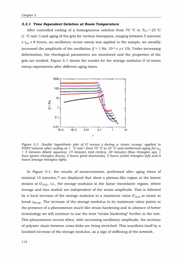
Chapter 5

112

5.3.1 Time Dependent Gelation at Room Temperature

After controlled cooling of a homogeneous solution from 70 °C to Tiso = 25 °C

(1 °C min-1) and aging of the gels for various timespans, ranging between 5 minutes

≤ tiso ≤ 8 hours, an oscillatory strain sweep was applied to the sample; we steadily

increased the amplitude of the oscillation (f = 1 Hz, 10-4 ≤ γ ≤ 10). Under increasing

deformation, the rheological parameters are monitored and the properties of the

gels are studied. Figure 5-1 shows the results for the storage modulus G' of strain

sweep experiments after different aging times.

Figure 5-1. Double logarithmic plot of G' versus γ during a strain sweep, applied to P3HT/toluene after cooling at 1 °C min-1 from 70 °C to 25 °C and isothermal aging for tiso

= 5 minutes (black squares), 15 minutes (red circles), 30 minutes (blue triangles up), 1 hour (green triangles down), 2 hours (pink diamonds), 5 hours (violet triangles left) and 8 hours (orange triangles right).

In Figure 5-1, the results of measurements, performed after aging times of

minimal 15 minutes,19 are displayed that show a plateau-like region at the lowest

strains at G'LVE, i.e., the storage modulus in the linear viscoelastic regime, where

storage and loss moduli are independent of the strain amplitude. This is followed

by a local increase of the storage modulus to a maximum value G'max at strain at

break γbreak. The increase of the storage modulus to its maximum value points to

the presence of a phenomenon much like strain hardening and in absence of better

terminology we will continue to use the term “strain hardening” further in the text.

This phenomenon occurs when, with increasing oscillatory amplitude, the sections

of polymer chain between cross-links are being stretched. This manifests itself by a

localized increase of the storage modulus, as a sign of stiffening of the network.


113

Further increase of the oscillatory amplitude beyond γbreak rapidly disrupts the

network which is revealed by the drop of the signal. At the end of each sweep, the

last data points of each series indicate that the sample did not return to its

homogeneous state. A “residual” modulus value was observed at the end of the

experiment. From visual observation of the gel, it appears to consist of smaller gel

domains dispersed in a more homogeneous solution phase.

With aging time, the LVE storage modulus G'LVE increases while the maximal

strain at break γbreak decreases. We observe a gradual evolution of gel stiffness with

time. The time dependence of the rheological parameters will be discussed further

in the following sections.

The influence of the oscillatory frequency on the rheological behavior was

assessed by performing the same measurements at different oscillation

frequencies. Figure 5-2 shows partial results of these measurements, where over 2

orders of magnitude (0.1 Hz ≤ f ≤ 10 Hz) no clear frequency dependence of the

storage modulus in the LVE regime could be observed. The data point for f = 0.1 Hz

and after tiso = 15 minutes is likely located higher due to the increased

measurement time required at smaller frequencies. Frequency independent

behavior was also observed for the other rheological parameters.

Figure 5-2. Frequency dependence of G'LVE over 2 orders of magnitude for aging at Tiso= 25 °C and cooling at 1 °C min-1. Timespans tiso: 15 minutes (red circles), 30 minutes (blue

triangles up), 1 hour (green triangles down), 2 hours (pink diamonds), 5 hours (violet triangles left) and 8 hours (orange triangles right). Dotted lines represent average values.

Chapter 5

114

5.3.2 Influence of Mild Changes in Thermal History

Now, we expand the rheological analysis of the gelation in P3HT/toluene by

varying the following parameters which define the thermal history of the samples:

cooling ramp (1, 5 °C min-1) and aging temperature (Tiso = 25, 30 °C).

Homogeneous solutions at 70 °C were subjected to different temperature

profiles, followed by an aging interval at Tiso (ranging between 5 minutes ≤ tiso ≤ 8

hours). After the aging step, the storage modulus G' was recorded during a strain

sweep experiment (f = 1 Hz), increasing γ from 10-4 to 10. We include the results

discussed in Section 5.3.1 in this comparison.

In analogy to the previous section, we define three characteristics from the

strain sweep experiments, G'LVE, G'max and γbreak, which enable us to reconstruct

the properties of the gel as a function of time. In Figure 5-3, the results of the four

sets of measurements are presented. The increasing value of G'LVE with aging time

demonstrates a long term evolution of the gel. The break point at strain γbreak is

reached at smaller amplitudes with increasing aging time, which can be related to

a lower molar mass between cross-links. As the gel ages further, the average length

of the sections of chain between cross-links become shorter and the sections can

withstand less strain. Therefore, we can state here that with aging time, the

network is characterized by higher modulus values and increased stiffness, while it

can endure less strain and will break at smaller deformation.

Figure 5-3. Plot showing the time dependence of the following characteristics: G'LVE (a, closed symbols), G'max (a, open symbols) and strain at break γbreak (b, closed symbols)

for the different sets of measurements: Tiso = 25 °C and cooling at 1 °C min-1 (black

squares), Tiso= 25 °C and cooling at 5 °C min-1 (red circles), Tiso= 30 °C and cooling at 1 °C

min-1 (blue triangles up), Tiso= 30 °C and cooling at 5 °C min-1 (green triangles down).


115

Comparing the four chosen experimental conditions, we have made the

following observations regarding the influence of the isothermal aging temperature

and the thermal history of the solution (i.e., the cooling rate). The gels with the

largest stiffness are formed by cooling the homogeneous P3HT/toluene solution to

25 °C at a rate of 1 °C min-1 (Figure 5-3, black squares). After 8 hours, a plateau is

reached at a G'LVE value about two orders of magnitude larger than the starting

value measured after 5 minutes. A faster cooling rate of 5 °C min-1 results in a

similar time evolution, but with lower absolute values for the moduli (red circles)

reached in the same time interval.

Isothermal evolution of the gel at 30 °C results in different behavior (blue and

green triangles). The gels are formed slower and a plateau of stable gel morphology

is anticipated only at longer times. The modulus values are significantly smaller

and the gels are much less extensible than what was observed at 25 °C.

5.3.3 Rheological Behavior for P3HT Gels formed at Tiso = 5 °C

In Chapter 4 we reported on the phase behavior of P3HT and we presented the

partial phase diagram of P3HT-99P/toluene (Figure 4-10b). During both cooling

and heating of the solutions, two thermal transitions were identified. Considering

the location of these transitions and the accessible temperature range in the

rheology setup, an aging temperature Tiso of 5 °C was selected with aging times tiso

from 10 minutes up to 8 hours. With a temperature ramp of 1 °C min-1, we

imposed the identical time-temperature profile on the sample during rheology and

DSC measurements. We opted for a different rheology approach in this section; no

amplitude sweep but monitoring of the dynamic moduli during the entire

temperature cycle (cooling, isothermal aging and heating). From the measurements

described in the previous sections, we were able to choose oscillation parameters

within the linear viscoelastic regime of the formed gels (f = 1 Hz, γ = 0.01).

In Figure 5-4 we show the rheological response, in the form of storage and loss

moduli G' (black) and G'' (red), for a sample aged at 5 °C for 5 hours. We will

describe the general features of the rheology runs observed in Figure 5-4 and

discuss the aging time dependent behavior.

Cooling the sample down, the polymer solution shows only a loss component

(G'') until at approximately 23 °C the storage response crosses the loss component.

Following the work of Winter et al., the cross-over between G' and G'' is defined as

Chapter 5

116

the gel point Tgel (sol-gel transition).20 This is accompanied by a rapid increase of

the moduli by several orders of magnitude (e.g., in this experiment 3 orders of

magnitude for ΔT ≅ 5 °C). This indicates the formation of a percolating network of

P3HT, between the inner and outer cylinder of the measurement cell.

During the isothermal period, we observed a drop in the modulus values, which

is in direct contrast to the reconstructed time dependency during aging at 25 °C

(Figure 5-3). This might be due to the more pronounced bleeding of the gel at this

(lower) aging temperature, creating a small lubrication layer of solvent between the

gel and rheometer. Therefore, this part of the rheology curve will not be considered

in the discussion.

Figure 5-4. Storage G' (black) and loss modulus G'' (red) versus temperature with an iso-

thermal period of 5 hours at 5 °C (arrows indicate the direction in which the experiment was conducted).

Reheating the gel, hysteresis becomes apparent. We observe a two-step process

in the decrease of the dynamic moduli. Around Tδ = 30-35 °C a local peak is

present in the loss modulus signal (or in tan δ ). This is followed by a regime

showing viscoelasticity, with storage and loss moduli approximately equal to one

and other (tan δ ≅ 1). The gel-sol transition is defined at the temperature where G'

drops definitively below G''; in Figure 5-4 at Tsol = 42 °C. At higher temperatures,

the sample is gradually returned to its homogeneous state, characterized by only

the loss component and a similar viscosity as at the beginning of the experiment,

here at dissolution temperature Tdis = 61 °C.


117

Rheology experiments performed with different aging times showed the same

features as discussed above in the case of tiso = 5 hours: during cooling, crossing of

G' and G'' at Tgel ≈ 23 °C, followed by a large and rapid increase of the moduli;

decrease of the signal during the isothermal period (the extent of which could not

be correlated to the aging time); a two-step process during heating containing a

small local peak at Tδ = 30-35 °C, followed by a temperature region showing

viscoelastic behavior prior to Tsol ≈ 45 °C and final dissolution at Tdis ≈ 60 °C. The

temperature ranges in which these characteristics can be observed seem

unaffected by the applied aging time. Therefore, we must conclude that the

rheological data do not show definite aging time dependence, for this aging

temperature.

5.3.4 Thermal Analysis of the Gel Samples

The thermal behavior of P3HT/toluene solutions was first described in this

thesis in Chapter 4, where we presented partial phase diagrams limited to low

polymer mass fractions. Two endothermic transitions were observed during

heating. Here, we further investigate the thermal behavior with DSC by performing

aging experiments at 25 °C, and in the second part of this section we discuss

experiments with Tiso = 5 °C.

For comparison with the rheology results, we controlled the thermal history of

the samples by applying a temperature profile like in the previous Section 5.3.1,

i.e. cooling from 70 °C to 25 °C at 1 °C min-1 and isothermal aging for timespans of

5 minutes ≤ tiso ≤ 8 hours. At the end of the applied isothermal period, the samples

are quenched to 5 °C to better visualize both endothermic transitions during the

subsequent heating (to 70 °C at 1 °C min-1). The thermograms during heating are

shown in Figure 5-5.

We label the transition temperatures consistent with the definitions proposed in

Chapter 4. The small endothermic signal of the first transition, with maximum Tm,i

around 28 °C, is comparable for all aging times. In the temperature range 45-

65 °C, we notice a significant trend with aging time. After tiso = 10 minutes, we

observe a small exothermic transition followed by a wider endothermic peak. This

could point to a reorganization event, prior to the final dissolution of the gel. With

longer aging times, the enthalpy change of the wider endothermic process

increases significantly. After tiso of 5 and 8 hours, the exothermic transition is no

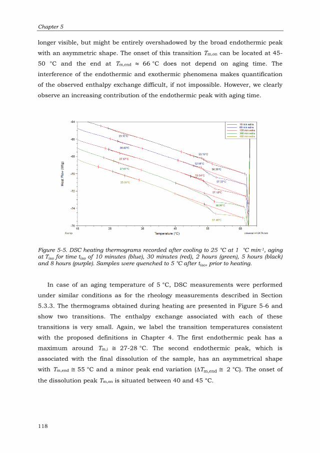
Chapter 5

118

longer visible, but might be entirely overshadowed by the broad endothermic peak

with an asymmetric shape. The onset of this transition Tm,on can be located at 45-

50 °C and the end at Tm,end ≈ 66 °C does not depend on aging time. The

interference of the endothermic and exothermic phenomena makes quantification

of the observed enthalpy exchange difficult, if not impossible. However, we clearly

observe an increasing contribution of the endothermic peak with aging time.

Figure 5-5. DSC heating thermograms recorded after cooling to 25 °C at 1 °C min-1, aging at Tiso for time tiso of 10 minutes (blue), 30 minutes (red), 2 hours (green), 5 hours (black)

and 8 hours (purple). Samples were quenched to 5 °C after tiso, prior to heating.

In case of an aging temperature of 5 °C, DSC measurements were performed

under similar conditions as for the rheology measurements described in Section

5.3.3. The thermograms obtained during heating are presented in Figure 5-6 and

show two transitions. The enthalpy exchange associated with each of these

transitions is very small. Again, we label the transition temperatures consistent

with the proposed definitions in Chapter 4. The first endothermic peak has a

maximum around Tm,i ≅ 27-28 °C. The second endothermic peak, which is

associated with the final dissolution of the sample, has an asymmetrical shape

with Tm,end ≅ 55 °C and a minor peak end variation (∆Tm,end ≅ 2 °C). The onset of

the dissolution peak Tm,on is situated between 40 and 45 °C.


119

Figure 5-6. DSC thermograms recorded during heating after aging at Tiso 5°C for time tiso of 10 minutes (blue), 30 minutes (red), 2 hours (green), 5 hours (black) and 8 hours (purple). Indicated from left to right are Tm,i, Tm,max and Tm,end.

The transition temperatures Tm,i are independent of both aging temperature and

time. The final melting temperature Tm,end is not related to aging time, but is

situated at a considerably lower temperature in case of Tiso = 5 °C, in comparison

to samples aged at Tiso = 25 °C; Tm,on is shifted down about 5 °C due to the lower

aging temperature. Samples subjected to an aging temperature of 25 °C, show time

dependent changes in both rheology (moduli values) and thermal analysis (much

larger and increasing ∆Hm). An aging temperature of 5 °C, however, does not show

this kind of behavior. These experimental observations seem to suggest that an

ambient gelation temperature allows changes in the network to take place. At a

temperature as low as 5 °C, the mobility of the chains might be too restricted or

the changes in the sample are not detectable with the analysis techniques.

For the latter set of measurements (Tiso = 5 °C), we can compare the transition

temperatures determined from rheology and DSC analyses. Figure 5-7 shows that

in both the rheological and the DSC data, there is no significant trend which

relates the isothermal aging time to the transition temperature. Therefore, no aging

time dependence is apparent, as can be seen from the distribution of measurement

points around the solid and dashed lines, representing the respective transition

temperatures averaged over tiso.

Rheology and DSC are analysis techniques which probe very different sample

properties. It is therefore not our intention to interpret the absolute temperature

Chapter 5

120

difference between the different transition temperatures. For example, Tsol refers to

the melting of the gel, i.e. the network covering the gap between both cylinders of

the measurement cell, while Tm,end indicates the final dissolution of all P3HT

aggregates discernable with DSC. We therefore added Tdis as the temperature

where the viscosity of the solution is returned to its initial value, i.e. of the

homogeneous solution. The absolute temperature difference between these two

parameters is due to the high sensitivity of viscometric techniques to the final

dissolution temperature of a polymer solution.21 Also the large volume of the

rheology sample in comparison to the small DSC sample can contribute to the

temperature difference between both estimations. The presence of both Tδ and Tm,i

in a fairly narrow temperature range (∆T ≅ 5 °C ) indicates that these two transition

temperatures could also be an expression of the same transition phenomenon.

However, we must conclude that overall, we do not possess conclusive

information on the nature of the transitions during the dissolution/melting of the

gels.

Figure 5-7. Transition temperatures and their average, determined from rheology (open,

dashed) and DSC (closed, solid) versus tiso.

5.3.5 In-Line Rheology – SANS: Analysis of the Network Structure

In the previous sections, we focused on macroscopic properties of P3HT gel

samples by studying the rheological and thermal responses. By measuring small

angle neutron scattering (SANS) during the gelation at ambient temperature, we

can obtain information at smaller length scales (initial gel formation and further

evolution with time). Moreover, the combination with rheology in-line, allows a


121

direct comparison of the time/temperature dependent behavior from two

perspectives.

The P3HT/toluene-d8 solution (wP3HT-99P = 0.01) was loaded in the concentric

cylinder of the rheometer and homogenized at 70 °C for 1 hour. Under continuous

oscillation (f = 1 Hz, γ = 10-2, rheological parameters chosen in the LVE region

based on Section 5.3.1), the homogeneous solution was cooled down to Tiso= 20 °C

(approximately 1 °C min-1) and kept isothermally for tiso = 10 minutes and 4 hours

for the different experiments. Afterwards, the sample temperature was gradually

increased to 70 °C, where the sample returns to the initial solution state.

As stated in the experimental section on SANS, the q-range of interest was only

accessible through the combination of three different instrument settings where

the neutron wavelength 𝜆 and the sample-to-detector distance were adjusted.

Therefore, every experiment (time-temperature cycle) had to be conducted three

times to record the scattering patterns under the different instrument settings. The

rather poor temperature control made it difficult to precisely repeat the same

experimental conditions. However, we were able to correlate the data sets and

obtain the complete SANS patterns for the majority of the time/temperature

experiments. The experimental problems we experienced regarding the temperature

control are described in the Appendix to Chapter 5.

5.3.5.1 In-line Rheology

Performing rheology experiments in-line, enables the direct comparison of

changes with time and temperature in the SANS data with the gel properties. In

Figure 5-8, we plot the response of the storage modulus G' (black) and loss

modulus G'' (red) versus temperature (a) and versus time for the isothermal period

(b). The data shown here was recorded during an experiment with tiso = 4 hours,

with SANS sample-to-detector distance of 8 m and is considered representative for

the other rheology runs.

During cooling, we observe a steep increase of the moduli between

30 °C > T ≥ 20 °C. In the subsequent isothermal period, the value of G' continues

to increase as shown in (b), approaching but not reaching a limiting value over the

course of 4 hours. The heating part of the measurement cycle shows two regimes.

Chapter 5

122

Initially during heating, the storage modulus even increases leading up to a local

peak with maximum approximately 30 °C. At higher temperatures, G' decreases

gradually. Due to the lower sensitivity of the apparatus used in the in-line

experiments, we were unable to obtain reliable rheology data for the sol-gel

transition temperatures and dissolution of the gel. Nevertheless, in-line and in-

house rheology data are in agreement and we can therefore use the in-house

results when more detailed information is needed.

Figure 5-8. Storage G' (black) and loss modulus G'' (red) versus temperature (a) and time

for tiso = 4 hours (b).

5.3.5.2 Small Angle Neutron Scattering

In comparison to the measurements discussed in Chapter 2, the measurements

in this series are i) limited at the high q side (q ≤ 0.0856 Å-1 versus q ≤ 0.52 Å-1 in

Chapter 2) and ii) data in the homogeneous solution state in the low momentum

transfer range, recorded with neutron wavelength 𝜆 = 13 Å, show much more

scatter due to the shorter acquisition time and lower signal-to-noise ratio (SNR).

The signal-to-noise ratio is not a problem in the gelled state as the scattered

intensity is orders of magnitude larger than in the solution state. Hence, we are

able to measure at lower q-values and therefore, larger real space dimensions.

Figure 5-9 shows an overlay of representative SANS patterns corresponding to

different time-temperature conditions during the experiment (cooling and aging at

Tiso = 20 °C). In the first SANS profile obtained at 40 °C (black), we see a clear

scattering pattern at higher q (data at smaller q suffering from low SNR, was not

represented). After cooling to 30 °C (red), the intensity has increased slightly and

there is a beginning larger contribution at lower q. With further decrease of the


123

temperature, the scattered intensity increases tremendously and we see the

development of two regimes with different slopes.

Figure 5-9. Overlay of SANS patterns during cooling recorded at 40 °C (black), 30 °C (red),

26 °C (blue), 24 °C (green), 20 °C at t0 (pink) and 20 °C at tiso = 10 minutes (orange). Data with insufficient SNR is not represented.

As the behavior of P3HT is reversible with temperature, we obtain similar

scattering patterns during the heating part of the experiment. Due to hysteresis of

this process, the relative temperatures at which similar scattering patterns are

obtained are shifted to higher values. At the end of the temperature cycle, the

sample is again a homogeneous solution.

Literature on P3HT structure formation in solution, describes the aggregation of

the polymer chains into semi-crystalline nanowires1 and also in fully developed

P3HT organogels (tiso > 24 hours at room temperature) such fibrillar nano-

structures have been observed.13,22 In reference 13, e.g., Newbloom et al. have used

a summation of the contributions of two phases (according to their estimated

volume fraction) to describe the scattering curve in the higher q-range: semi-

crystalline nanofibrils (modeled by a parallelepiped shape) and amorphous single

chains still in solution (modeled as a polymer with excluded volume interactions).

At lower q, analysis of the SANS pattern proceeds via a power law, describing the

network according to its fractal dimension D, which relates to the scattered

intensity as

I(q) ∝ q -D (5.1)

Chapter 5

124

The measurements on which we report here, are performed on significantly

shorter time scales and our data indicate that we do not have such well-defined

nanowires in our gelled samples. In Figure 5-10 we show cryo-TEM images of

P3HT/toluene gels which represent a projection of the morphology in situ, inside

the bulk of the gel, by rapidly vitrifying a small volume of the gel in liquid nitrogen.

The images are taken after an aging time of 1 hour at 30 °C and 20 °C. There are

no pronounced semi-crystalline nanowires visible in these images. The respective

2D low-dose electron diffraction (LDED) patterns show the presence of P3HT in the

field-of-view by a diffuse band, but not like a well-defined ring or, after radial

averaging of the LDED pattern, a sharp peak associated with the reflection of the

π-π stacking in the P3HT nanowires. In the images we can see a density contrast

between the P3HT-enriched phase (dark) and P3HT-poor phase in the vitrified

solvent layer (light), with the density differences becoming more outspoken at lower

temperature. Also in situ synchrotron wide angle X-ray diffraction (WAXD)

experiments on our samples did not show evidence of crystalline P3HT.

Figure 5-10. Cryo-TEM images of 1 wt% P3HT/toluene samples after 1 hour at tiso = 30

and 20 °C. Scale bar 0.2 μm.

Given the inhomogeneous two-phase morphology, we can better think of the

P3HT/toluene system in the initial stages of gel formation as consisting of a set of

(uncorrelated) P3HT-enriched domains embedded in a P3HT-depleted matrix.

Shibayama et al. have used a Ornstein-Zernike-like (OZ) approach in their study

on poly(vinyl alcohol)-borate gels, representing the total scattered intensity I(q) by23

I(q) = IOZ(0)

{1+[(Df+1)

3⁄ ]ξ2

q2}Df 2⁄ + Iex(0) exp[-(q Ξ)α] (5.2)

The first term in Equation 5.2 represents the generalized Ornstein-Zernike-like

(OZ) contribution to the scattered intensity, arising from the internal structure of

30 °C 20 °C


125

the P3HT-enriched domains, which are characterized by fractal dimension Df and

correlation length ξ or effective correlation length ξ ' = [(Df+1)

3⁄ ]

1 2⁄

ξ. The excess

scattering at lower q is taken into account by the addition of a stretched

exponential function defined by Ξ and 𝛼 , as proposed by Geissler et al.24 to

accommodate the (uncorrelated) distribution of the polymer-rich blobs. Here, Ξ

represents a second correlation length (Ξ > ξ ') linked to the distribution of polymer-

rich domains throughout the sample.

Equation 5.2 is capable to provide a quantitative fit of our SANS data over the

measured q-range. In Figure 5-11, we show a representative scattering pattern,

recorded at tiso = 2.5 hours, and the fit according to Equation 5.2 (red solid line).

The two terms are also represented separately, by the dashed line for the OZ-type

contribution and the dotted line for the stretched exponential function.

Figure 5-11. SANS pattern recorded at tiso = 2.5 hours with the fits according to Equation 5.2 (red solid). The separate contributions are shown by the dashed (Ornstein-Zernike-

like) and dotted lines (stretched exponential).

We have analyzed the scattering patterns recorded at different time-

temperature conditions by fitting Equation 5.2. In Figure 5-12, we show the

change of the 6 fitting parameters versus isothermal aging time and in Figure 5-13

versus temperature, to show the changes during heating: scattered intensity at

q = 0 IOZ(0) (a), intensity at q = 0 Iex(0) (b), effective correlation length ξ ' =

[(Df+1)

3⁄ ]

1 2⁄

ξ (c), correlation length Ξ (d), fractal dimension Df (e) and exponent 𝛼

Chapter 5

126

(f). Data from the experiments with tiso = 10 minutes is represented in black and tiso

= 4 hours in red.

Figure 5-12. Change of fitting parameters versus isothermal aging time: scattered

intensity IOZ(0) (a) and Iex(0) (b), correlation lengths ξ' = [(Df + 1) 3⁄ ] 1 2⁄

ξ (c) and Ξ (d), fractal

dimension Df (e) and exponent 𝛼 (f). Measurements with tiso = 10 minutes (black closed

symbols) and tiso = 4 hours (red, open).

In the first part of the measurement cycle during cooling, in the temperature

window 30 °C > T ≥ 20 °C, changes in the scattering patterns occur quickly (see

Figure 5-9), much like the behavior in the rheological experiments. We observe a

rapid increase of the scattering intensity IOZ(0) and Iex(0) as the network is being

formed. The fractal dimension Df of the P3HT-enriched domains increases as well,


127

while an opposite trend occurs for the associated effective correlation length ξ '. At

the larger length scale, the correlation length Ξ increases and the exponent 𝛼

decreases. The trends continue throughout the beginning of the isothermal period

(~30 minutes), as shown in Figure 5-12.

After ~30 minutes of isothermal aging, IOZ(0) no longer changes (Figure 5-12a)

while the rate of change for ξ ' and Df slows down (c,e). A quantitative interpretation

of Df is not unique, as deviations of a value of 2 are often found in networks,

however, with usually Df > 2 for more compact morphologies. We observe an

increase of Df during isothermal aging and a (slightly) higher maximum value (Df ~

2.55) for gels formed with longer aging times. The decrease of the effective

correlation length leads to a minimum value in the range of ξ ' ~ 180 Å.

The parameters of the stretched exponential contribution (representing the

behavior at larger length scales in the inhomogeneous P3HT/toluene samples) are

not affected by isothermal aging for longer times (> 30 minutes). Approximate

values for the P3HT gel are Ξ ~ 1000 Å and 𝛼 ~ 1, the latter making this an

exponentially decaying correlation in reciprocal space.

During the subsequent heating (Figure 5-13), the intensity IOZ(0) first remains

fairly constant, then steadily decreases between ~ 30 °C and 50 °C, and more

rapidly at higher temperatures. For the stretched exponential, we observe a

continuous lowering of intensity Iex(0), initiated at approximately 30-35 °C until the

contribution of this exponential function disappears at T > 55 °C, with Iex(0) → 0.

Up to 50 °C, the correlation length Ξ decreases only slightly with increasing

temperature, while ξ ' and Df remain unaffected. Above 50 °C all three parameters

change more abruptly. The exponent 𝛼 of the stretched exponential contribution

shows a minor change up to 40 °C, above which 𝛼 is gradually affected more with

increasing temperature.

Moreover, looking in detail, the difference in absolute value of Df and ξ ' between

the two applied aging times becomes gradually smaller during initial heating, as we

observe a mild continued evolution for Df,10min and ξ '10min

up to approximately

45 °C (Figure 5-13c,e). This observation points to the further growth of the

Chapter 5

128

aggregates with time, during heating, in experiments with a short effective aging

time (time interval at Tiso, tiso = 10 minutes).

Figure 5-13. Change of fitting parameters versus temperature (heating): scattered

intensity IOZ(0) (a) and Iex(0) (b), correlation lengths ξ' = [(Df + 1) 3⁄ ] 1 2⁄

ξ (c) and Ξ (d), fractal

dimension Df (e) and exponent 𝛼 (f). Measurements with tiso = 10 minutes (black closed

symbols) and tiso = 4 hours (red, open).

5.3.5.3 Combining SANS, Rheology Observations and Thermal Analysis

With the information from both characterization techniques gathered in-line, we

can now provide a better interpretation of the transitions described above. Where

appropriate, we also include rheology data presented earlier in this chapter and

thermal analysis data.


129

Cooling the homogeneous P3HT solution, the onset of the formation of the gel is

determined around 30 °C. Regarding rheology, the gel point is estimated to be

about 30 °C (using the method of Winter et al.20), after which the storage modulus

of the sample increases over 3 orders of magnitude. In the SANS patterns in Figure

5-9, we see the first indications of change at 30 °C, followed by a rather sudden

and abrupt evolution of scattered intensity (can be qualitatively seen in Figure 5-9),

which is reflected by the steep rate of change of the parameters determined from

the SANS pattern, by Equation 5.2, in the temperature range 30 °C > T ≥ 20 °C.

During the first ~30 minutes of the isothermal period, the dynamic moduli and the

parameters we used to describe the SANS pattern, all continue to increase (except

ξ ', 𝛼: decrease) at a high rate.

After 30 minutes, the SANS fitting parameters IOZ(0), Iex(0), Ξ and 𝛼 , have

reached a limiting value and do not show significant change at longer tiso. The time

dependence of the fractal dimension Df (Figure 5-12e) and the effective correlation

length ξ ' (Figure 5-12c) is seen to be very similar: a strong increase/decrease up to

tiso ~ 30 minutes followed by an evolution at a gradually lower rate. Also for the

storage modulus G', we observe an evolution at a gradually reduced rate towards a

limiting value (not yet reached after 4 hours, see Figure 5-8b). This time dependent

behavior is very comparable to the aging time dependence of G'LVE (at Tiso = 25 °C)

we discussed in Section 5.3.2 (Figure 5-3a); that data was obtained from amplitude

sweeps without applying deformation during isothermal aging.

Rheology experiments performed in-house (Tiso = 25, 30 °C, Figure 5-3a) and in-

line (Tiso = 20 °C, Figure 5-8b) show a clear evolution of the storage modulus

during isothermal aging, as also reported in literature.13 Conversely, in Section

5.3.3, we discussed the time-temperature rheology experiments performed in-

house with Tiso = 5 °C, where a decrease of storage and loss moduli during the

isothermal period was observed and which could not be directly correlated to aging

time. At this time, we cannot provide a definite explanation for the decreasing

modulus with aging time. If bleeding of the gel occurs at Tiso = 5 °C, a phenomenon

where solvent is expelled from the network, this creates a thin lubrication layer

between the gel and the concentric cylinders of the rheometer. The recorded moduli

then no longer represent directly the network characteristics.

Chapter 5

130

During subsequent heating, we observe various dependencies of the SANS

fitting parameters with temperature. The intensity of the lower q-region, Iex(0)

shows the fastest and most significant decrease, initiated at ~30 °C, occurring at a

fairly constant rate and approaching zero at T > 50 °C. IOZ(0) also decreases for T >

30 °C, but by a faster rate of change at T > 50 °C. A similar two-step decrease upon

heating can be seen for Ξ and 𝛼. Df and ξ ' on the other hand, remain constant up

to ~55 °C (Df,10min and ξ '10min

even marks a continued evolution due to shortened

effective aging time), after which they show rapid changes. We can state that with

increasing temperature, the changes occur first at the larger length scales, before

the internal configuration of the (denser) P3HT-rich domains is affected.

In DSC, the enthalpy exchange associated with the second endothermic

transition also shows aging time dependence at ambient Tiso (Figure 5-5). The

increasing contribution of this transition with tiso enables us to assign it to the final

dissolution of the P3HT-rich clusters in the gel.

5.3.6 The Proposed P3HT Network Morphology and its Temperature

Dependence

We propose a model of gel formation and dissolution for P3HT/toluene(-d8)

solutions as shown in Figure 5-14. Upon cooling of the sample, we reach the sol-

gel point and observe the formation of a heterogeneous structure at the largest

length scale (correlation length Ξ) observed in our SANS experiments, consisting of

a P3HT-depleted matrix phase and P3HT-enriched domains. Furthermore, we pick

up the internal structure of the P3HT-rich domains, characterized by ξ ' and Df and

acting as cross-links of the network. The effective correlation length ξ ' ~ 180 Å is

smaller than the estimated contour length of the polymer (Ln = 220 Å). Therefore,

given the rather large PDI of the P3HT polymer, chains are long enough to connect

domains and form an interconnected network in the P3HT-enriched phase.

Moreover, also at the larger lengths scale in the P3HT-depleted matrix phase a

network is formed, connected to the enriched domains. The correlation length at

this scale, Ξ ~ 1000 Å, is larger than the number average contour length Ln of

P3HT. It therefore must be the small number of polymer chains with high molar

mass in the broad distribution that take care of the connectivity in the P3HT-

depleted matrix phase and the connection to the P3HT-enriched domains, i.e. the

long polymer molecules in the broad molar mass distribution take part in the


131

cross-links in the P3HT-enriched domains, creating a volume spanning

heterogeneous network, which is similar to a bimodal polymer network made up of

end-cross linked short and long chains.

Figure 5-14. Schematic representation of the P3HT gel during the initial stages of formation, showing the P3HT-depleted (light) and P3HT-enriched (darker) phases (Ξ), the latter containing P3HT cross-link clusters (characterized by Df and ξ').

The elasticity of bimodal networks under small deformation has been reported

in literature to be dominated by the short polymer chains in the network.26 The

P3HT gel can be considered as such a bimodal network consisting of P3HT-

enriched and -depleted domains (larger length scale network, correlation length Ξ),

with the former containing internal structure at a smaller length scale (cross-link

domains, effective correlation length ξ '), which effectively determines the elasticity

(G') of the network.

According to basic ideal rubber theory,25 the elastic modulus is inversely

proportional to the molar mass between cross-links Mc, i.e. G = ρRT Mc⁄ with ρ the

network density, R the ideal gas constant and T the absolute temperature. This

equation can also be applied to the elastic modulus of thermoreversible gels or to

the storage modulus of these gels, representing the elastic component of the

complex modulus of such gels, i.e. G' ∝ 1 Mc⁄ ∝ 1 ξ '⁄ , where we assume that the

effective correlation length ξ ' is a measure for Mc of the shorter chains in the

Chapter 5

132

bimodal network. In Figure 5-15, we show the linear dependency between G' and Df

and 1/ξ ' . The similar rate of change of these parameters illustrates that the

changes at the smaller length scale, i.e. inside the P3HT-enriched domains, are

responsible for the increased gel strength at the macroscopic level (storage

modulus). The increasing value of Df can be interpreted to point to a gradual higher

density of the P3HT-rich phase with time. Simultaneously the change of ξ '

indicates that the molar mass between cross-links decreases. Therefore, with aging

time, the P3HT-enriched domains show internal changes, as they densify and the

P3HT-enriched cross-link domains come closer together.

Figure 5-15. Plot of the storage modulus during isothermal aging for 4 hours at 20 °C versus Df and 1/ξ′, showing linear dependency.

The growth of the network continues for ~30 minutes at Tiso = 20 °C, with

increasing modulus values, scattered intensities and correlation length Ξ . The

polymer-enriched phase becomes denser, contracts and the cross-linked domains

come in closer proximity of each other. The macroscopic elasticity of the P3HT gel

is controlled by the smaller length scale of the bimodal network. Also when the

growth of the network seems to stop, the further increase of the storage modulus is

due to continued internal evolution of the P3HT clusters (Df, ξ ').

Subsequent heating of the P3HT gel leads firstly to the disappearing of the

larger scale correlation (equivalent of the gel-sol transition), while samples with

short aging times mark a slight continued evolution of the P3HT-rich domains

internally. Only at higher temperatures the remaining polymer clusters start to


133

disappear, which can be interpreted as the dissolution of the sample towards the

homogeneous P3HT/toluene(-d8) solution.

5.4 Conclusions

While homogeneous at high temperature, P3HT/toluene solutions form a gel

when stored at room temperature. We investigated the gelation behavior of samples

with wP3HT = 0.01 by performing time and temperature dependent measurements

(varying the isothermal aging temperature Tiso and time tiso) with complementary

characterization techniques: rheology, DSC and SANS. The gel formation and

development are firstly studied with rheology and we observe the influence of the

thermal history of the sample (Tiso and cooling speed) on the gel properties.

Cryo-TEM images of gelled samples show an inhomogeneous two-phase

morphology at room temperature. Small angle neutron scattering (SANS) and

rheology data combine to the following description of the gelation behavior. Upon

cooling the homogeneous solution, a heterogeneous morphology of a P3HT-

depleted matrix phase and P3HT-enriched domains containing cross-linked

clusters is formed , effectively forming a bimodal network. After crossing the sol-gel

point, the network structure grows rapidly during further cooling and aging at Tiso

= 20 °C for ~ 30 minutes.

We showed a continued increase of the moduli when applying longer aging

times (up to 8 hours), due to internal changes of the polymer-rich phase as the

density increases and the molar mass between cross-links (effective correlation

length ξ ') becomes smaller, while at the larger length scale of the P3HT-enriched

and P3HT-depleted phases no changes occur ( Ξ , 𝛼 ). The SANS data can be

interpreted to give a measure of the molar mass between cross links Mc of the short

chains in the bimodal network, which are known to be able to dominate the elastic

modulus of bimodal networks. Indeed, a unique one-to-one correspondence

between the correlation length ξ ', characterizing the P3HT-enriched domains, and

the storage modulus G' of the formed network has been established.

Increasing the sample temperature, the P3HT-enriched phase with cross-link

domains remains unchanged (or continues to evolve slightly when short applied

aging times). The spatial correlation at large distances disappears and the gel-sol

transition temperature is crossed. At higher temperatures, the P3HT-clusters also

dissolve and the sample returns to the homogeneous solution state.

Chapter 5

134

References

1. Berson, S., De Bettignies, R., Bailly, S. and Guillerez, S. Poly(3-hexylthiophene) Fibers for Photovoltaic Applications. Adv. Funct. Mater. 17, 1377–1384 (2007).

2. Chen, C., Chan, S., Li, J., Wu, K., Chen, H., Chen, J., Huang, W. and Chen, S. Formation and Thermally-Induced Disruption of Nanowhiskers in Poly(3-hexylthiophene)/Xylene Gel Studied by Small-Angle X-ray Scattering. Macromolecules

43, 7305–7311 (2010). 3. Koppe, M., Brabec, C. J., Heiml, S., Schausberger, A., Duffy, W., Heeney, M. and

McCulloch, I. Influence of Molecular Weight Distribution on the Gelation of P3HT and its Impact on the Photovoltaic Performance. Macromolecules 42, 4661–4666 (2009).

4. Malik, S., Jana, T. and Nandi, A. K. Thermoreversible Gelation of Regioregular Poly(3-hexylthiophene) in Xylene. Macromolecules 34, 275–282 (2001).

5. Kitts, C. C. and Vanden Bout, D. A. The Effect of Solvent Quality on the Chain Morphology in Solutions of Poly(9,9′-dioctylfluorene). Polymer 48, 2322–2330 (2007).

6. Huang, P., Chang, Y. and Chou, C. Preparation of Porous Poly(3-hexylthiophene) by Freeze-Dry Method and its Application to Organic Photovoltaics. J. Appl. Polym. Sci. 122,

233–240 (2011).

7. Kim, B.-G., Jeong, E. J., Park, H. J., Bilby, D., Guo, L. J. and Kim, J. Effect of Polymer Aggregation on the Open Circuit Voltage in Organic Photovoltaic Cells: Aggregation-Induced Conjugated Polymer Gel and its Application for Preventing Open Circuit Voltage Drop. Appl. Mater. Interfaces 3, 674–680 (2011).

8. Malik, S. and Nandi, A. K. Influence of Alkyl Chain Length on the Gelation Mechanism of Thermoreversible Gels of Regioregular Poly(3-alkyl thiophenes) in Xylene. J. Appl. Polym. Sci. 103, 2528–2537 (2007).

9. Berghmans, H. in Integration of Fundamental Polymer Science and Technology (eds.

Lemstra, P. & Kleintjens, L.) p 296 (Elsevier Applied Science: London, 1988). 10. Keller, A. in Structure Properties Relationship of Polymeric Solids (ed. Hiltner, A.) p 25

(Plenum Press: New York, 1983).

11. Tipton, D. L. and Russo, P. S. Thermoreversible Gelation of a Rodlike Polymer. Macromolecules 29, 7402–7411 (1996).

12. Arnauts, J. and Berghmans, H. Amorphous Thermoreversible Gels of Atactic Polystyrene. Polym. Commun. 28, 66–68 (1987).

13. Newbloom, G. M., Weigandt, K. M. and Pozzo, D. C. Electrical, Mechanical, and Structural Characterization of Self-Assembly in Poly(3-hexylthiophene) Organogel Networks. Macromolecules 45, 3452–3462 (2012).


15. Richards, J. J., Weigandt, K. M. and Pozzo, D. C. Aqueous Dispersions of Colloidal Poly(3-hexylthiophene) Gel Particles with High Internal Porosity. J. Colloid Interface Sci.

364, 341–350 (2011). 16. Lindner, P. and Schweins, R. The D11 Small-Angle Scattering Instrument: A New

Benchmark for SANS. Neutron News 21, 15–18 (2010). 17. Lindner, P. Neutrons, X-rays and Light: Scattering Methods Applied to Soft Condensed

Matter. Chapter 2 (Elsevier, 2002).

18. Imae, T., Kanaya, T., Furusaka, M. and Torikai, N. Neutrons in Soft Matter. 393–394

(John Wiley and Sons, Inc., 2011). 19. For shorter aging times, no plateau but an increase of G’ with oscillatory amplitude was

observed. This is due to the time scale of isothermal aging versus the measurement duration.

20. Winter, H. H. and Chambon, F. Analysis of Linear Viscoelasticity of a Crosslinking Polymer at the Gel Point. J. Rheol. 30, 367–382 (1986).

21. Kramer-Lucas, H., Schenck, H. and Wolf, B. A. Influence of Shear on the Demixing of Polymer Solutions, 1 Apparatus and Experimental Results. Makromol. Chemie 189,

1613–1625 (1988). 22. Newbloom, G. M., Kim, F. S., Jenekhe, S. A. and Pozzo, D. C. Mesoscale Morphology and

Charge Transport in Colloidal Networks of Poly(3-hexylthiophene). Macromolecules 44,

3801–3809 (2011).


135

23. Shibayama, M., Kurokawa, H., Nomura, S., Muthukumar, M., Stein, R. and Roy, S. Small-Angle Neutron Scattering from Poly(vinyl alcohol)-borate Gels. Polymer 33, 2883–

2890 (1992).

24. Mallam, S., Horkay, F., Hecht, A. M. and Geissler, E. Scattering and Swelling Properties of Inhomogeneous Polyacrylamide Gels. Macromolecules 22, 3356–3361 (1989).

25. Treloar, L. R. G. The Physics of Rubber Elasticity. (Oxford University Press, USA, 2005).

26. Seetapan, N., Fuongfuchat, A., Sirikittikul, D. and Limparyoon, N. Unimodal and

Bimodal Networks of Physically Crosslinked Polyborodimethylsiloxane: Viscoelastic and Equibiaxial Extension Behaviors. J. Polym. Res. 20, 183 (2013).

136

137

APPENDIX to Chapter 5

A5.1 In-Line Rheology - SANS: Temperature Control

Small angle neutron scattering information over the desired momentum

transfer range 8.7 × 10-4 ≤ q ≤ 0.0856 Å-1 was obtained by combining three

scattering patterns, each recorded with different instrument settings. Variations in

the experimental conditions within one set of data can have negative implications

on the feasibility of matching of the partial scattering patterns. Having separate

software controls over the temperature for the rheological part of the experiments

and the SANS experiments, we made a considerable effort to perform the

experiments as synchronized as possible. The temperature, however, showed

unwanted and, at the moment of the experiments, unresolved variations. In Figure

A5-1 we show two time-temperature plots (tiso = 10 minutes, a; tiso = 4 hours, b) as

the profiles were recorded by a thermocouple in the cell. The programmed profile is

represented by the dashed line, while the measured temperature is given by the

solid line (the onset of the isothermal period defined at t0). On the left we can see a

clear difference between the effective heating rates of the three runs; in Figure A5-

1b, we observe a deviation of the isothermal aging time. Because of the lack of

synchronization of the different signals, a detailed manual matching of the different

SANS profiles and rheology data had to be performed.

Figure A5-1. Representative time-temperature profiles comparing the planned profile (dashed) with the experimental profiles (solid) for experiments with tiso = 10 minutes (a) and tiso = 4 hours (b).

138

139

EPILOGUE

In the final part of this thesis, we summarize first the highlights of this work,

arranged per topic. Then, we broaden our view gradually and discuss our

approach, the research project and a general outlook in conclusion of this

dissertation.

Fundamental Chain Parameters

We performed a detailed characterization of a set of poly(3-hexylthiophene)

polymers (varying in molar mass, molar mass distribution and regioregularity), by

conventional techniques (molar mass by SEC, regioregularity (RR) by 1H NMR) and

by means of small angle neutron scattering (SANS). The latter provided an

independent determination of Mw, ⟨Rg2⟩z and Lp.

Comparing the molar mass estimates by the two characterization techniques

confirms the significant overestimation of Mw by SEC (calibrated with PS), which is

due to the absence of a SEC calibration method suitable for these semi-flexible

polymers. Nonetheless, when molar mass information is provided in literature, it

generally consists of SEC results. This is the result of the restricted accessibility of

SANS or other scattering techniques with absolute measure of intensity. However,

researchers should be aware of the bias on reported molar mass values.

The radius of gyration was shown to scale with chain length as

⟨Rg2⟩1 2⁄ ∝ N 0.66 ± 0.04, with N the number of bonds. By means of simulation, we

were able to establish that the exponent is the effect of a combination of stiffness

and excluded volume (EV) interactions. For the chain lengths and chain stiffness

values considered, the effect of stiffness is the most important and excluded

volume alters the scaling behavior only slightly with a few to maximum 10%, the

excluded volume effect would become more important at higher chain lengths.

Epilogue

140

Persistence length values ranging 35 Å ≤ Lp ≤ 60 Å were determined for the

different P3HT polymers. We furthermore presented the linear relationship between

persistence length Lp and P3HT regioregularity. Therefore, low-RR P3HT shows

different behavior of at the level of structure formation, where defects hamper

crystallization by steric hindrance and planarization difficulties, as well as at the

single chain level of these semi-flexible polymers, with intrinsic chain stiffness

function directly of regioregularity. The Holtzer approach, used to experimentally

determine Lp, was validated by simulation, with proportionality constant C = 3.6 ±

0.2 in Lp = C q⁄ *; in good agreement with C = 3.5 as proposed in the literature.

Semi-Flexible Excluded Volume Polymers

Configurational-bias Monte Carlo (cbMC) simulations of semi-flexible hard

sphere chains (SFHSC) predict the size and persistence length as a function of

number of bonds in the linear chain N and stiffness (angular bending constant kb).

Longer chains are affected more by excluded volume interactions, leading to larger

⟨R 2⟩, ⟨Rg2⟩ and Lp. With increasing stiffness, the contribution of EV will diminish

and the chain properties gradually approach the results of the ideal SFC (slower

decay for larger N). In the form factor P(q) excluded volume interactions are present

at lower q-values (larger real space dimensions) for longer chains and with

increasing stiffness. Like the size and persistence of the chain, at high stiffness the

form factor is not affected by excluded volume.

The systematic simulation approach focused on a range of chain length and

stiffness (N ≤ 200, kb ≤ 40), and as a result, we obtained a library of fundamental

chain properties and dependencies for short semi-flexible chains without and with

excluded volume interactions. A theory, which accounts for both semi-flexibility

and the excluded volume effect and predicts fundamental chain properties, is

currently not available for these polymer chains. Therefore, the matrix of chain

parameters composed in this work, can serve as a tool to the initial estimation of a

range of fundamental chain characteristics (from, e.g., Mw and Lp as experimental

input).

In the research presented in Chapter 3, the chain bending stiffness is evenly

distributed over the simulated polymers. In the case of P3HT specifically, however,

chain stiffness is the determined also by regiodefects, i.e. non-head-to-tail bonds,

Epilogue

141

which cause a kink in the chain. Only with information on the distribution of the

defects over the polymer chain, a more realistic ensemble of chains can be

produced, parameterized by, e.g., two bending constants representing the different

linkages. This, as well as the consideration of polydispersity, can lead to simulation

results for P3HT as a SFHSC in closer agreement with experimental values.

However, without the construction of these detailed ensembles, we have already

provided a good estimation of the fundamental chain parameters of P3HT modeled

according to the SFHSC model.

Phase Behavior

The tendency of regioregular P3HT chains to assemble into semi-crystalline

nanowires inspired us to investigate the crystallization and melting behavior of

P3HT as function of RR, by DSC. We showed that the melting temperature Tm of

P3HT polymers with molar mass above a threshold value (Mn ≅ 6.5 kg mol-1) is not

affected by regioregularity (shown for RR ≥ 95%). Shorter chains are characterized

by a lower Tm due to a 1/Mn dependency, but more importantly, are affected by the

regioregularity of polymer. Regiodefects along the polymer chain reduce the length

of the crystallizable segments and effectively limit the crystal thickness.

In solution, P3HT structure formation has been shown upon decreasing the

solvent quality, e.g., by lowering the sample temperature. We established binary

phase diagrams of P3HT/toluene (or ODCB), with several exo- and endothermic

transition temperatures. The melting point depression with RR shows 2 groups,

similar to the behavior of the powder P3HT samples. The crossing of melting lines

for P3HT/toluene and P3HT/ODCB, suggest the internal structure of P3HT

aggregates is an effect of the solvent of choice. In contrast to ODCB, low

concentrations of RR-P3HT (wP3HT = 0.01) form a gel in toluene at room

temperature.

P3HT/Toluene Gels

The formation, growth and dissolution of RR-P3HT/toluene gels was studied

with rheology, SANS and DSC. Time and temperature dependent aging experiments

reveal rapid formation of a network upon cooling, which continues to grow during

initial aging (~30 minutes) at ambient Tiso. Cryo-TEM images indicate an

inhomogeneous two-phase morphology of P3HT-depleted and P3HT-enriched

Epilogue

142

domains, the latter becoming more dense throughout gel development and with

cross-link clusters inside growing in closer proximity of each other. The elasticity of

these bimodal networks is dominated by the internal structure of the P3HT-

enriched domains at a smaller length scale (cross-link domains).

Gradual heating of the gelled sample leads in a two-step process to the gel-sol

transition (~ 50 °C), without affecting the internal structure of the P3HT-enriched

domains. Higher temperatures ensure the complete dissolution of the remaining

P3HT dispersion. Both the cooling rate during structure formation and the applied

aging temperature influence the macroscopic gel properties as reflected in the

dynamic moduli.

Structure Formation of P3HT in Toluene

Photoactive layers of P3HT/PCBM organic solar cells are generally made from a

homogeneous solution of donor and acceptor in organic solvent. Upon deposition

and layer drying, semi-crystalline nanowires of P3HT are formed, which are

beneficial for the device efficiency, and a post-processing thermal annealing step

can be used to further optimize the photoactive layer morphology. Overall,

processing conditions have a large impact on the morphology, crystallinity and

final device efficiency.

P3HT aggregates or precursors also develop in solution upon decreasing solvent

quality. Structure creation and layer deposition may then be decoupled by the

formulation of an ink consisting of pre-formed P3HT nanostructures. This could

diminish the impact of processing conditions (e.g., deposition method, drying time)

on the final layer morphology and, furthermore, the thermal annealing step could

be modified to a milder process (which is applicable to flexible substrates).

The stability of the ink is an important consideration, permitting storage of the

dispersions for limited time spans (preferably at ambient temperature). For

deposition methods such as inkjet or roll-to-roll printing, which are often proposed

in the context of low-cost large-scale production, a certain viscosity range needs to

be respected. Structure creation in low-polymer content P3HT/toluene solutions,

which was the focal point in this study, does not respect these boundary

conditions: we observed a large viscosity increase upon storage at ambient

temperature and a continuous evolution of the morphology of the samples.

Epilogue

143

However, reports in literature have also pointed out the potential benefits of a gel

morphology regarding, for example, the conductivity of charges.

Toluene was selected as the solvent of choice in this research, in spite of the

general preference for CHCl3 or ODCB, which are yielding better efficiency results,

but because of possibilities in the industrial use of non-halogenated solvents in

eventual solar cell production. Toluene, however, is not considered the optimal

solvent choice, since it is still prone to heavy regulations when used in an

industrial production process.

In the organic solar cell literature, poly(3-hexylthiophene) has been profiled as a

model donor material and was used in a wide variety of studies dealing with, e.g.,

solar cell efficiency or photo-active layer morphology versus donor-acceptor ratio,

casting solvent, P3HT molar mass, P3HT regioregularity or processing conditions.

The ability of P3HT to form both semi-crystalline nanowires in solution and an

extended network, depending on the conditions, renders the behavior of this

polymer complex. Therefore, in hindsight P3HT might not be a typical or true

model donor material for polymer solar cells. Nonetheless, it is clear that the

collective ensemble of studies on P3HT has provided the organic solar cell research

community with paramount information and insight, useful in, e.g., the

development of new materials with improved intrinsic properties and the

optimization of processing conditions for other materials.

144

145

ACKNOWLEDGEMENTS

Here I am sitting behind my laptop with just this final piece to write. With all

the previous pages done, you would think that the toughest is now behind me. But

after all, the acknowledgements section is the perfect place to express gratitude. So

I am smiling while I realize that the difficulty is because I have been surrounded by

so many wonderful and inspiring people while working at TU/e and living in

Eindhoven. I am truly thankful for every one of you who has walked this path with

me.

First of all, I am indebted to my promotors prof.dr. E.L.F. Nies and prof.dr. G.

de With. Erik, I consider you my most important mentor and guide. Since I first

followed your lectures on polymers during my Bachelor studies in Leuven, I have

found the energy with which you teach inspiring and energizing. Our discussions

always left me with a peak in motivation and I want to sincerely thank you for

sharing your knowledge with me, for your patience, your positive outlook, and for

having confidence in me.

Bert, I cannot express how thankful I am for the opportunity to pursue my PhD

degree in SMG. Being a part of your group has given me so much more than I

could have imagined. Thank you for your genuine interest in my research, for

always taking the time to think with me and sharing your perspectives. While never

losing attention for detail, you helped me to also keep the larger picture in mind.

I also want to thank the committee members for sacrificing their valuable time

to read and comment on my thesis and for taking part in my defense ceremony.

Especially to prof.dr.ir. R.A.J. Janssen, Rene, an additional thank you for

welcoming me to the lunch meetings and to the solar cell device lab, where I could

learn more about organic solar cells. To the people of ECN and especially dr. S.

Veenstra, Sjoerd, thank you for your interest in my part of our project and for your

advice and answers to my questions.

Acknowledgements

146

I am thankful to the Dutch Polymer Institute for funding my research project

and for offering a great platform of knowledge exchange as well as exchange of

experience. I would like to thank John van Haare in particular.

During the first few years of my PhD studies, I spent also quite some time as a

guest researcher at the KULeuven. Therefore, I would like to thank all the people of

the Division of Polymer Chemistry and Materials, especially dr. Ting Li for teaching

me so much about simulations, dr. Filip Meersman for joining my first trip to

Grenoble and Marcel Lasker for taking care of all things technical. Also the Master

students who worked with me on their graduation project for their dedication,

contribution to my research and for allowing me to learn from them: thank you

Bram Vanroy, Ellen Bertels and Lies Eykens.

I have always considered doing measurements in Grenoble as a highlight and I

will remember these times as a great opportunity. I am thankful to the people of

the DUBBLE beam line at ESRF and instrument D11 at ILL, for their guidance and

support.

Within SMG, I have been lucky to find so much more than a professional work

place with pleasant colleagues. My gratitude goes to the scientific and technical

staff of SMG for creating a kind and friendly atmosphere where you are both

supported and challenged. Thank you dr. Catarina Esteves (also for sharing the

office), prof.dr. Nico Sommerdijk (I greatly value your time and input during our

progress meetings), dr. Jos Laven (for your help with the rheometer experiments),

dr. Frank Peeters (for advice on my early simulations, although they did not make

it into this thesis), dr. Heiner Friedrich, dr. Sasha Kodentsov (for your advice on life

and amazing stories), dr. Günther Hoffmann, prof.dr. Rolf van Benthem and dr.

Leo van der Ven. Marco Hendrix, for your friendship, creative support in the design

of the cover and so much more, Huub van der Palen always everything with a

smile, Paul Bomans, Niek Lousberg and Ingeborg Schreur-Piet. The first member of

SMG to welcome me into the group, Imanda, you have been a continuous

immediate support with the paperwork we all so dislike taking care of, and thank

you also for guarding the group atmosphere and taking interest in our lives.

Among my (PhD) student and post-doc colleagues in SMG, I have made some of

my best friends. Experiencing similar hardships and difficulties, and sharing them,

Epilogue

147

we got to know each other very well. But the unforgettable moments and happy

memories have enriched my life far more than I could imagine. During the daily

coffee breaks, Thursdays in the FORT, monthly SMG borrels and so many more

occasions, I have been surrounded by genuinely wonderful people. I appreciate all

of you deeply and your friendship is the best reward of all. Thank you, Ana

(Saudades! I’ll see you in Brazil), Aroa, Baris, Beulah (you are a truly inspiring

person), Beryl, Camille (always helping me to see the silver lining, with and without

wine), Cansu, Cem (doctor2), Delei (the master chef! and so much more), Dina,

Eldhose, Eva, Giulia, Gokhan, Hesam (my caring friend), Indu, João, Jos, Kangbo,

Karthik (almost my twin brother), Katya (for the kind atmosphere in the office),

Koen(tje), Kyrill, Laura, Lijing, Maarten, Marcel (Sabbelke?), Marcos (manneke!!),

Mark (for your appreciation of my Belgian-ness and for sharing/spinning the

wheel), Maurizio, Nasir (thank you for your hard work and nice contribution to my

thesis), Oana (with unlimited energy), Paul, Peter, Qingling (you are one of the most

warm-hearted people I know), Sasha A., Vladimir (with your beautiful family and

unprecedented presentation skills), Yogesh, Yujing, Zihui... SMG, What Else?!

An additional and very special thank you to my paranimphen Baris and

Maarten. Baris, my dear friend, although you left Eindhoven already some time

ago, I never get the feeling that you are truly far away! Thank you for supporting

me, always. Maarten, working with you on this project, made me feel like I was

never alone. You were always ready with advice, for a talk about everything and

nothing and your genuine friendship means so much to me. You have become a

scientist and person who I admire in many ways.

At the end of any working day, there were always friends around to spend the

evening with, go on little trips or in general, just have a relaxing good time. I met so

many of you in Eindhoven during these past years, and I am grateful for every one

of you and all the time we got to spend together. Thanks to you, Eindhoven has

always felt like home. Cheers to all of you, Alberto, Antonio, Ard, Benjamin and

Florence, Camille D., Carlos, Catalina, Daniele D., Daniele R., Dario, Domenico,

Dominik, Enrico, Evgeniy, Ezequiel, Ivelina and Nico, Jason, Maria, Martin,

Matthieu, Mindaugas, Mylene, Paulo, Raymond, Sami… I look forward to visiting

you, wherever you might end up!

To my friends from Leuven, who all already earned their doctor’s degree in the

meantime, thank you for your support, Brecht, Elke, Katrien, Pieter and Ruben.

Acknowledgements

148

A special thank you to my softball friends. We have known each other now for

many years, (almost) like sisters, and our friendship has been the perfect

“distraction”. I am even more happy about all the visits I got in Eindhoven! Femke,

Karen, Nathalie and Sophie, you are always my champions. Thank you also, coach

John Corley.

My dear family, thank you for always being there and for everything. Moeke en

vake, dank jullie om alles met mij te willen delen, van de warme gezelligheid thuis

tot mijn ups en downs, werk en vriendschappen in Eindhoven, altijd paraat om

„wel eventjes tot ginder te komen“. Frederic, ik ben blij dat ik mijn studies altijd

met jou heb kunnen delen, van samen de slappe lach krijgen aan tafel tijdens de

blokperiode tot serieuze discussies over polythiofenen. Ik ben enorm fier dat jij de

volgende doctor in onze familie zal worden! Jouw doorzettingsvermogen is ongezien

en ik kijk nog steeds op van alles wat je blijft bereiken. Olivier, ik bewonder jouw

creativiteit en musicaliteit, oprechte hart en brede interesse. Jij haalt echt alles uit

het leven met als terechte beloning een ton aan ervaringen waarover ik je zo graag

hoor vertellen. Zonder jullie aanmoediging, steun en hulp zou ik hier niet geraakt

zijn. Ik geniet ervan om nu thuis zo dicht bij jullie aan mijn volgende hoofdstuk te

beginnen.

Isabelle

149

CURRICULUM VITAE

Isabelle Monnaie was born on December 14th, 1986 in Antwerp, Belgium. After

finishing her studies at the Damiaan Instituut Aarschot, Belgium in 2004, she

studied Chemistry at the Katholieke Universiteit Leuven (KUL), Belgium. In 2008,

as part of her Master’s degree, she carried out a six-month industrial internship at

Philips Research, in Eindhoven, the Netherlands, working on a project entitled

“Development of Functionalized Materials for Tissue Engineered Heart Valves”

under the supervision of dr. D. Halter. She then returned to Leuven to complete

her graduation project entitled “Properties of P3HT in Solution: Towards High-

Performance Polymer Solar Cells by Controlling Active Layer Morphology” in the

Division of Polymer Chemistry and Materials, supervised by prof.dr. E.L.F. Nies

and subsequently obtained her Master’s degree in Chemistry (magna cum laude) in

2009. In August 2009, Isabelle joined the Laboratory of Materials and Interface

Chemistry at the Eindhoven University of Technology, the Netherlands, where she

started her PhD project under the supervision of prof.dr. E.L.F. Nies and prof.dr.

G. de With. The doctoral research was funded by the Dutch Polymer Institute (DPI),

project 682 “Creation of Functional Nanostructures in Solution/Dispersion”. The

most important results of this research are presented in this dissertation.

Documents

Structure creation of P3HT in solution - Pure - … Isabelle Structure Creation of P3HT in Solution The work described in this thesis forms part of the research program of the Dutch