Master Thesis in Geosciences

Structure and Microseismicity of the unstable rock slide at Åknes, Norway

Marianne Holst Nielsen

2

Structure and Microseismicity of the Unstable Rock slide at Åknes, Norway

Marianne Holst Nielsen

Master Thesis in Geosciences

Discipline: Petroleum Geology and Geophysics

Department of Geosciences

Faculty of Mathematics and Natural Sciences

UNIVERSITY OF OSLO 15th of December 2008

3

© Marianne Holst Nielsen, 2008 Tutor(s): Valerie Maupin (University of Oslo, Blindern), Isabelle Lecomte (NORSAR, Kjeller & ICG, Oslo), Michael Roth (NORSAR, Kjeller & ICG, Oslo This work is published digitally through DUO – Digitale Utgivelser ved UiO http://www.duo.uio.no It is also catalogued in BIBSYS (http://www.bibsys.no/english) All rights reserved. No part of this publication may be reproduced or transmitted, in any form or by any means, without permission.

4

Abstract The Åknes site is a potential rockslide in a hillside of a fjord on the west coast of Norway in the county of Møre Og Romsdal. A rockslide at Åknes has the potential of making a large flood wave. The flood wave could destroy the closest villages and kill many people. Due to this big threat the area has been heavily investigated by numerous methods since it was discovered in 1985 by NGI. Among these investigations a passive seismic network for monitoring the microseismicity of the area was temporarily installed in 2005, recording seismic data for 6-7 weeks. The dataset from this acquisition has been analyzed in this thesis. 7 microseismic events have been detected with an algorithm which uses the STA/LTA method. From the information on five shots of a refraction seismic survey executed the last two days of the passive networks recording period, has been used to make a traveltime-distance plot for the whole area. From this plot a velocity model has been made. By using the relation between traveltime and epicentral distance, found from the five shots, the detected events have been localized by using a misfit function. Sammendrag På Åknes i Møre og Romsdal, Norge, er det i dalsiden av en fjord oppdaget et potensielt fjellskred. Et ras på Åknes kan lage en enorm flodbølge nede i fjorden. Denne flodbølgen vil ødelegge de nærmeste bygdene og mange menneskeliv vil gå tapt. Området ble i 1985 først undersøkt av NGI. På grunn av den potensielle faren fra Åknes, så har området siden den gang blitt grundig undersøkt med mange ulike metoder. Blant disse undersøkelsene ble det i 2005 utplassert midlertidig et passivt seismisk nettverk for å undersøke områdets mikroseismisitet. Nettverket registrerte seismisiteten i 6-7 uker. Datasettet fra denne undersøkelsen er blitt analysert i denne oppgaven. Det er blitt funnet 7 mikroseismiske hendelser i dataene ved å bruke en algoritme som benytter seg av STA/LTA metoden. I løpet av de to siste dagene av registreringstiden til det passive nettverket ble det utført refraksjonsseismikk med fem aktive skudd. Informasjon om disse skuddene er brukt til å lage et gangtid-avstandsplott som omfatter hele området. Fra dette plottet er det laget en hastighetsmodell. Ved å bruke forholdet mellom gangtid og episentrisk avstand, som ble funnet i gangtid-avstansplottet, så har man ved hjelp av en mistilpassningsfunksjon lokalisert de seismiske hendelsene.

5

CONTENT: Page nr: 1: INTRODUCTION...............................................................................................................8

1.1: Rockslides in western Noway.................................................................................8 1.2: Åknes.......................................................................................................................8 1.3: Gathering of passive seismic data.........................................................................12 1.4: Objectives..............................................................................................................15

2: DETECTING EVENTS…………….................................................................................16 2.1: Method for detecting events…..............................................................................16 2.1.1: The STA/LTA method............................................................................16 2.1.2: Algorithm for detecting events...............................................................17 2.2: The detected events…………...............................................................................23 3: VELOCITY MODEL........................................................................................................38 3.1: Traveltime-distance plot from dynamite blasts.....................................................38 3.2: The velocity model................................................................................................41 3.3: Uncertainty concerning the location of the geophones.........................................44 4: LOCALIZATION..............................................................................................................49 4.1: Determination of the best slope plane...................................................................49 4.2: Method for localization.........................................................................................50 4.3: Result from the localization of microevents.........................................................54 5: DISCUSSION.....................................................................................................................60 6: CONCLUSIONS................................................................................................................61 7: REFERENCES ..............................................................................................................63 APPENDIX A: matlab programs..........................................................................................66 APPENDIX B: Tables............................................................................................................77 APPENDIX C: Picking arrivaltimes……………………………………………………….87

6

1: INTRODUCTION

1.1: Rock slides in western Norway

The west coast of Norway is the land of the fjords. The fjords on the west coast of Norway

were created during periods with ice coverage in the Quaternary (from two million years ago).

Arms from the bigger inland ice have dug deep valleys into the bedrock, and the glacier

tongue has been in direct contact with the sea. Sediments transported by the ice created an end

moraine under the glacier tongue creating a shallow area as the ice melted and the sea flooded

the valley. The valleys are deep U-valleys with steep slopes at the sides filled with deep calm

blue/green tainted sea water. Because of the steep slopes and depending on the properties of

the soils and the bedrock in the area, many of these valleys have unstable rock masses in the

hillsides. This results in a constant occurrence of rock falls and slides of different sizes and

nature. Rock slides in some remote places would maybe do no significant damage, but rock

slides of the same size plunging into the fjords have the potential of making large flood

waves, which in turn are a threat to villages in the fjord valleys and users of the fjords. If you

drop a mass of stone into open waters, the energy of the resulting wave will spread out in a

3D hemisphere, but if you drop the same mass into a fjord, the energy from the resulting wave

will spread out in a 2D-like tube and the wave will have a height many times as high than in

open waters. Bathymetric measurement of the bottom of the fjords shows a history of rock

slides (Delarue, 2006). During the last century, rock slides and the following flood waves in

the fjords have killed 175 people (Delarue, 2006). In 1934 a rock fall at Langhammaren in the

Tafjord, Western Norway, killed 50 people and made enormous damages to three villages

(Furseth, 1985). The size of the rock masses of the 1934 slide was estimated to be about 3

million m3 and the flood wave had a maximum height of more than 60 m (Furseth, 1985).

1.2: Åknes

In the same area as the Tafjord, we have today a large potential rock slide at the Åknes site.

Among the areas that will suffer by a slide at Åknes is the Geiranger fjord which is one of

Norway’s largest tourist attractions. In high season the cruise ships practically wait in line to

sail in the fjord with thousands of tourists. Some of the ships even make a comment to the

7

tourists, while they sail past the Åknes site, of the danger hanging in the hillside. The

Geiranger Fjord was in 2005 put on UNESCO’s World Heritage List. Due to the threat to

people and nearby villages the Åknes site has been investigated by a number of methods since

1985, when the first geological mapping was carried out by NGI. The Åknes rockslide has

become one of the most investigated in the world, making it a naturally laboratory for

researches from all over the world. In the present study I will analyze microseismic data from

a temporary seismic network installed in 2005. This was installed just before another

permanent seismic network was installed, one which is operative today and which has been

studied by Michael Roth (NORSAR, Kjeller & ICG, Oslo, Norway). To get an overview of

the area to be studied I will introduce some details of the morphology and geology at the

Åknes site. Åknes is located in the same fjord system as the Tafjord, the Inner Storfjord

System on the west coast of Norway in the county of Møre og Romsdal. Figure 1.1 shows the

location.

Figure 1.1: The location of the Åknes site (Roth etal., 2006).

The flood wave created by a possible rockslide at Åknes would make a lot of material damage

and put many lives at risk. The size of the instable masses has been estimated to have a

volume of 35-40 million m3 (Darron etal., 2005). This is the estimation used in the latest

article (Ganerød etal., 2008), but there have been several estimations, some up to 100 million

m3. If this block should fall into the fjord in one piece, which is the worst case scenario, a

flood wave with a maximum height of 90m could be created (Eidsvig & Harbitz, 2005). If

you compare this to the volume of the Tafjord slide in 1934 you get an idea of the possible

damage a slide at Åknes would cause.

The instable area at Åknes is about 1 km2 and the slope is dipping towards south with

an average slope of 30-35˚ (Ganerød etal., 2008). Figure 1.2 shows a picture of the area taken 8

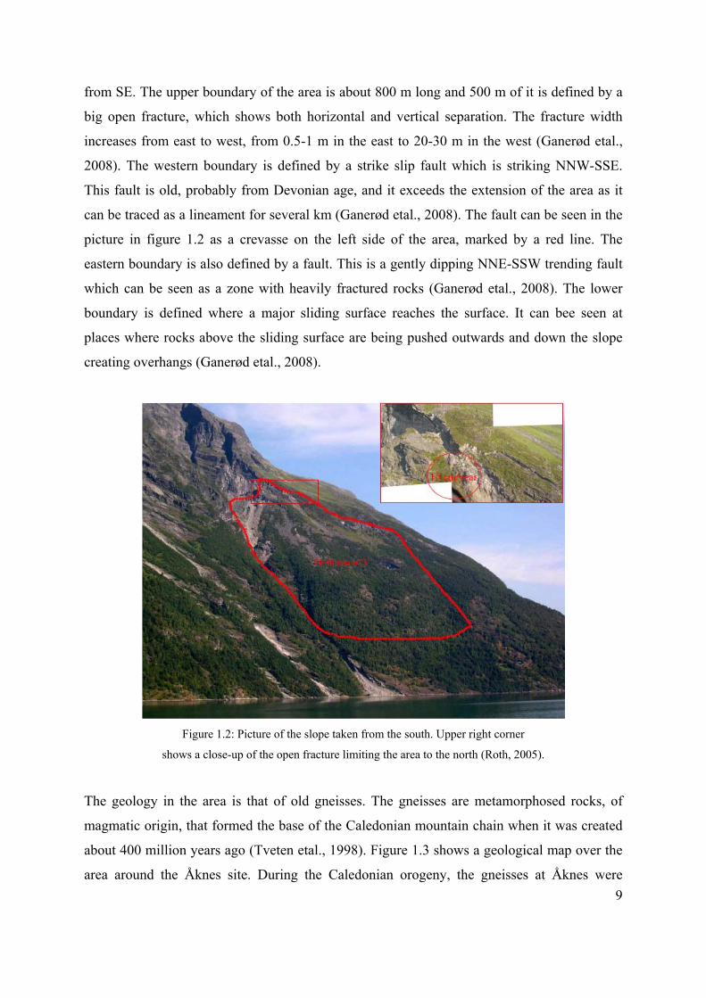
from SE. The upper boundary of the area is about 800 m long and 500 m of it is defined by a

big open fracture, which shows both horizontal and vertical separation. The fracture width

increases from east to west, from 0.5-1 m in the east to 20-30 m in the west (Ganerød etal.,

2008). The western boundary is defined by a strike slip fault which is striking NNW-SSE.

This fault is old, probably from Devonian age, and it exceeds the extension of the area as it

can be traced as a lineament for several km (Ganerød etal., 2008). The fault can be seen in the

picture in figure 1.2 as a crevasse on the left side of the area, marked by a red line. The

eastern boundary is also defined by a fault. This is a gently dipping NNE-SSW trending fault

which can be seen as a zone with heavily fractured rocks (Ganerød etal., 2008). The lower

boundary is defined where a major sliding surface reaches the surface. It can bee seen at

places where rocks above the sliding surface are being pushed outwards and down the slope

creating overhangs (Ganerød etal., 2008).

Figure 1.2: Picture of the slope taken from the south. Upper right corner

shows a close-up of the open fracture limiting the area to the north (Roth, 2005).

The geology in the area is that of old gneisses. The gneisses are metamorphosed rocks, of

magmatic origin, that formed the base of the Caledonian mountain chain when it was created

about 400 million years ago (Tveten etal., 1998). Figure 1.3 shows a geological map over the

area around the Åknes site. During the Caledonian orogeny, the gneisses at Åknes were 9

heavily foliated and folded. The gneisses vary from medium grained granitic gneiss to

hornblende/biotite bearing medium grained dioritic gneiss, and you can also find up to 20 cm

thick layers of biotite schist (Ganerud etal., 2008). At Åknes the foliation is subparallel to the

surface and all the lithologies are in layers parallel to the foliation. The sliding surface has

developed as a consequence of this geological setting together with the faults described

above, with sliding starting in the weakest layers of the foliation. The total block which is

moving can be divided into two smaller blocks with different rates of movement, one in the

NW corner with a moving rate of 7-20 cm/year, and one bigger one comprising the main part

of the area that moves 1-4 cm/year (Blikra, 2006). Figure 1.4 shows the two blocks with

different colours.

Figure 1.3: A geological map around the Åknes site, marked with a black square.

The pink in the map is diorittic to granittic gneiss and migmatits. The orange area

are eyegneiss, granite and folieted granite. The green area are amfibolite and glimmer

slate (NGU, 2008).

Figure 1.4: The instable are is divided into two smaller blocks,

the smallest one in purple and the bigger one in orange (Blikra, 2006).

10

1.3: Gathering of passive seismic data

In 2005 a permanent seismic network for monitoring the microseismic activity of the slope

was installed. Microearthquakes are defined as a local earthquake with a magnitude of less

than 2.5. This network consists of eight 3-component geophones installed in the upper part of

the area, covering about 250 m x 150 m (Roth elat., 2005). When the unstable masses at

Åknes move, they move in tiny steps which creats microseismic earthquakes. By measuring

the rate of microseismic activity, one can say something about the rate of movement in the

slide (Roth, 2006). This network is now incorporated in a warning system, so that if the

seismic activity suddenly should increase and one expects the slide to accelerate, the people

living in the villages in the area can get a chance to evacuate.

Another seismic network, covering a larger area, was installed temporarily in 2005.

This was done in a project called “Geophysics for investigation and analysis of large

landslides” which was started in 2005 by the researchers at NORSAR and ICG (International

Centre of Geohazard), in coorporation with french colleagues at LGIT (Laboratoire de

Géophysique Interne et Tectonophysique, Grenoble). The aim of the project was to share

mutual experience in the use of geophysics in landslides (Lecomte, 2006), and Åknes was a

natural laboratory for this project. The aim of the project was especially to work on

background seismic noise, microseismic monitoring and seismic tomography, to better model

the rupture surface and internal deformations and to better understand the movement pattern

of the unstable block (Lecomte, 2006). During a mission to the Åknes site, 19/8-05 to 6/9-05,

an IHR (Réseau d’Imagerie de Haute Résolution) network provided by LGIT was installed.

The network acquired passive seismic data continuously for 6-7 weeks and was also used for

a short refraction seismic experiment 15th to 18th of October 2005. After October the site is

inaccessible because of snow. All the data from the IHR network had for different reasons not

yet been processed and analyzed, except for the recordings of the refraction seismic (Frery,

2007). The first analysis of the passive seismic, i.e., the recording of the micro seismic

activity during these 6-7 weeks has been done during the work of this thesis.

The IHR network consisted of ten stations, each is having nine channels associated

with six one-component vertical geophones and one three-component geophone. Actually the

whole IHR system consists of 30 stations but the Åknes site is a difficult area to work in so

managing to deploy as much as 10 stations demanded a great effort. Figure 1.5 shows the

11

different elements of each station. The IHR stations have a new acquisition system made for

difficult hazardous sites, and have a large number of available recording channels and

wireless communication between the stations (Brenguier etal, 2005). The stations were spread

out as evenly as possible over the area as shown in Figure 1.6. The stations are mostly

organized with the three-component geophone in the centre and the vertical component

geophones in a star like pattern around it (every 60˚) with cables of 30 to 50m (Roth etal,

2006) The geophones are marked with red and green crosses in figure 1.5. The horizontal

positions of the sensors were measured by differential GPS with an error of less than 15cm.

and the elevation was taken from a high resolution digital elevation map made by an airborne

laser scanner in 2004 (Frery, 2007). The geophones where all shielded with plastic containers

to keep the temperature and to minimize noise from wind.

Figure 1.5: The elements of one station in the IHR network.

The stations were powered by a solar panel.

The white rod is the radio antenna (Roth etal., 2006).

From a temporarily seismic pilot installation in 2004 it was clearly seen that the frequencies

of the microseismic events are well above 10Hz (Delarue, 2006). So a high sampling rate was

needed, which the IHR system can provide, and the stations were set to record with a

sampling interval of 4 ms (Frery, 2007).

12

Figure 1.6: The deployment of the stations S1 to S10 with the geophones marked with red

and green crosses. The shots from the refraction seismic survey SP1 to SP5 in blue (Frery, 2007)

During the last mission, just before the IHR network was dismantled, a seismic refraction

survey was put up. This was done along a 470 m long line in the centre of the area, from an

altitude of 300m to 580m above see level (Roth etal., 2005). In figure 1.6 the shots are marked

in blue with SP1 to SP5. Figure 1.7 shows the seismic section from SP1. There is a clear

brake in the first arrivals for trace nr 12 at 0.1s, where the slowness of first arrival times starts

to increase. Otherwise the first arrival times change quite regularly with increasing offset.

This indicates a velocity model with at least two layers of different velocities, a layer with low

velocity on top over a layer with higher velocity (Roth, 2006). An interpretation on the

velocities from this survey will be used for comparison to the velocity model made I chapter 3

13

Figure 1.7: Seismic section of SP2 showing a break in the

arrival times for receiver 12 at 0,1sec (Dietrich et al. 2005)

1.4: Objectives

During the work of this thesis the passive seismic data gathered by the IHR network in 2005

were analyzed. The goal was to find microseismic events in the data that are associated with

the movement of the rock slide at Åknes. To do this a method for automatically finding the

events in the data needed to be developed. Microseismic events had then to be localized. If

events are found and successfully localized, something can be said about the nature of the

movement of the slide. By locating an event one can say where the slide is active. The final

goal is to use the rate of microseismic events to reveal where the movement rate is highest. If

the hypocentre (the depth and position of an earthquake) can be mapped, one could also

determine the detachment zone. Seismic data alone may not be enough to accurately

determine the detachment zone but together with resistivity measurement, GPR measurement,

seismic refraction and tomography, and borehole analysis, the result can be quite robust.

14

2: DETECTING EVENTS

2.1: Method for detecting events

The dataset was converted from its original form to SAC (Seismic Analysis Code) format by

Olivier Coutant at LGIT (Laboratoire de Géophysique Interne et Tectonophysique), Grenoble,

in May 2008. Each sac-file contains data for one hour (900000 sampling points) from one

component. Each station has one directory, each of these contains one directory for each day,

and each day-directory contains the sac-files for every hour. The title of each file contains

information about the data and time, the station nr and the component nr.

The full amount of data was approximately a half of a terra byte. That is a lot of data

and given the limited amount of time for the present work, it was not possible to analyse all of

the data. So it was necessary to make a reasonable selection on what data to analyse and what

to leave for later work. The first decision was to only use the data from the 11 hours during

night time, from seven in the evening to seven in the morning. The reason behind this

decision was that during daytime there was quite a bit of field work going on making a lot of

noise on the data, at the time of recording because of extensive activities at Åknes in 2005

with various investigations and well boring, in addition to helicopter transport. This gives 250

Gbytes to work with.

2.1.1: The STA/LTA method

STA/LTA is short for Short-term Average over Long-Term Average. The purpose of this

method is to automatically detect when the amplitude of the seismic signal suddenly

increases. The method works by going through the seismogram, calculating the average of the

amplitude over two different time windows, and when the ratio between these two averages

(called STA/LTA) exceeds a certain value a registration of the time is triggered. The method

is useful when the target events are not exclusively the ones with the biggest amplitude, and it

can also to some extent help to distinguish between different types of earthquakes (Trnkoczy,

1998). In this method there are five parameters to set:

15

STA-window duration in time

LTA-window duration in time

STA/LTA trigger threshold level

STA/LTA detrigger threshold level.

Relative position between the STA and the LTA windows

The first two parameters are the two time windows over which the average of the amplitudes

are calculated. STA is an average over a short time window and LTA is an average over a

long time window. The second two parameters are the value of ratios that trigger and

detrigger the registration of an event. When the STA/LTA exceeds a certain value (the trigger

threshold level), the time is registered as the beginning of an event. When the STA/LTA

reaches a value below detrigger threshold level, the time is registered as the end of an event.

The parameters need to be chosen carefully to fit the type of waveforms that are the target

events. The STA time window needs in general to be a few periods longer than the expected

dominant period of a target event (Trnkoczy, 1998). By choosing a short LTA we make the

trigger more sensitive to short lasting local events with high frequency. If you were to be

interested in long period low frequency earthquake signal, the LTA would need to be longer

(Trnkoczy, 1998).

When the LTA is much longer than the longest duration of an event it represents the

average background noise level, and will not be very sensible to sudden changes in the

amplitude (Ambuter & Solomon, 1974). The STA will quickly respond to an increase in

amplitude. As you move in steps across the seismogram, continuously calculating the STA

and the LTA, the STA/LTA will have a value close to one when there are no events, but it

will increase suddenly when an event occurs and the value of STA increases while the LTA

stays close to the same.

2.1.2: Algorithm for detecting events

The algorithm was divided into four parts:

Part 1) Convert the sac-files into proper format for the chosen programming language.

16

Part 2) Make a program that goes through the data using the STA/LTA method and register

the times of the events and the header-information in a matrix.

Part 3) Automatically run part 1) and 2) for several sac-files and write matrices with the

registered events in a file.

Part 4) Sort out the resulting files containing the registered events.

Part 1) Matlab was the programming tool I choose to use, since this is the tool I am most

familiar with. To read sac-files into matlab, an already existing program called rsac.m was

used (Thorne, 2004). This program formats the sac files into a matrix with three columns. The

first column holds the time values, the second one holds the amplitude values, and the third

one holds the header information. A figure can be made of the seismic trace by plotting the

time values vs. the amplitude values. The matrix was then used as input argument in the

program findevents.m which goes through the sac file using the STA/LTA method.

Part 2) The program findevents.m was written as a function with the sacfile-matrix and the

filenames of the sac-file as input arguments. The program can be found in appendix A.2.

It was important when making this program to have in mind the amount of data (250

Gb) to be processed, and to reduce computing time as much as possible on each sac-file. This

means among other things keeping the for-loops and if-tests as simple and as few as possible.

First the four STA/LTA parameters were determined according to the theory above

and from information of what is used on the permanent seismic network at Åknes (Roth,

personal communication). The local microseismic events most suitable for localization have

durations of less than two seconds (Delarue, 2006). So the parameters where set to:

STA time window = 0.25 s

LTA time window = 2 s

STA/LTA trigger threshold = 3

STA/LTA detrigger threshold = 3

The relative position in time of the short term window and the long term window had also to

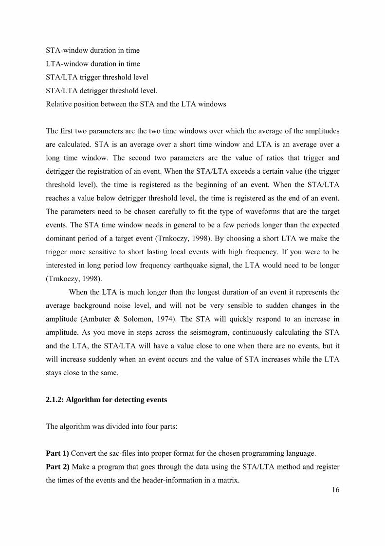
be chosen. There are two possible realative positions, as illustrated as line pieces in figure

2.2.1. One way is to let the STA end at the same time as the LTA ends. Another way is to let

the STA begin where the LTA ends.

17

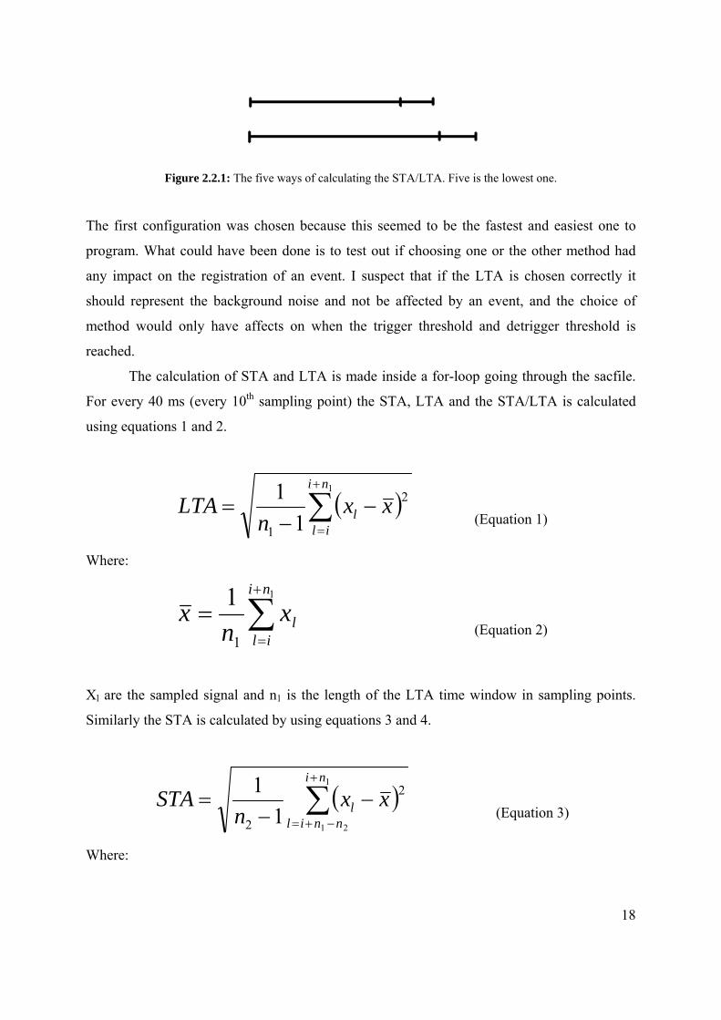
Figure 2.2.1: The five ways of calculating the STA/LTA. Five is the lowest one.

The first configuration was chosen because this seemed to be the fastest and easiest one to

program. What could have been done is to test out if choosing one or the other method had

any impact on the registration of an event. I suspect that if the LTA is chosen correctly it

should represent the background noise and not be affected by an event, and the choice of

method would only have affects on when the trigger threshold and detrigger threshold is

reached.

The calculation of STA and LTA is made inside a for-loop going through the sacfile.

For every 40 ms (every 10th sampling point) the STA, LTA and the STA/LTA is calculated

using equations 1 and 2.

( )∑+

=

−−

=1

2

1 11 ni

ill xx

nLTA

(Equation 1)

Where:

∑+

=

=1

1

1 ni

illx

nx

(Equation 2)

Xl are the sampled signal and n1 is the length of the LTA time window in sampling points.

Similarly the STA is calculated by using equations 3 and 4.

( )∑+

−+=

−−

=1

21

2

2 11 ni

nnill xx

nSTA

(Equation 3)

Where:

18

∑+

−+=

=1

212

1 ni

nnillx

nx

(Equation 4)

Where n2 is the length of the STA time window in sampling points. When calculating the

STA and LTA using equations 1 and 3 the mean amplitude is subtracted. The reason for this

is that the amplitude does not always oscillate around zero. Figure 2.2 shows an example of

this.

To be able to get a correct trigger time and a correct detrigger time compared to the actual

event, one might let the LTA stay constant from when trigger threshold is reached until

detrigger threshold is reached. This required an extra if-test inside the for-loop going through

the sacfile, and this element was dropped to save calculating time. To save even more time I

tried out to calculate the LTA outside the for-loop as an average of the whole sac-file and let

the value of LTA be constant when calculating the STA/LTA inside the loop. The idea was

that since the LTA is supposed to represent the background noise, it should not change

significantly through one sac-file, because it is only one hour long. But it turns out that the

noise level changes throughout the sac file. The result was triggering when there were no

event (where the background noise level decreased), and missing out events where the

background noise level increased compared to the amplitude of the event.

The final chosen configuration was to run, by going through the sac-file matrix every

10th sampling point, calculating the LTA, the STA and the STA/LTA. If the STA/LTA

exceeds the value 3, the time is registered in a matrix called “event” as the starting point of an

event, and when STA/LTA reaches a value below 3 the time is registered in the event matrix

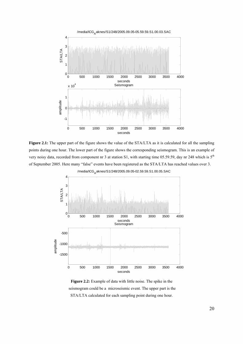
as the ending point of the same event. Figure 2.1 to 2.3 shows three examples of how the

STA/LTA varies during one hour and the corresponding seismogram. When the noise level

was high and contained a lot of spikes, many “false” events were registered as in figure 2.1.

On the noisiest days up to 20 “false” events were registered per hour. Figure 2.2 shows how

the STA/LTA reacts when a possible microseismic event is registered on the seismogram.

Figure 2.3 show that the STA/LTA also exceeds a value of 3 for local earthquakes.

19

0 500 1000 1500 2000 2500 3000 3500 40000

1

2

3

4

seconds

STA

/LTA

/media/ICGAaknes/S1/248/2005.09.05-05.59.59.S1.00.03.SAC

0 500 1000 1500 2000 2500 3000 3500 4000

-1

0

1

x 104 Seismogram

seconds

ampl

itude

Figure 2.1: The upper part of the figure shows the value of the STA/LTA as it is calculated for all the sampling

points during one hour. The lower part of the figure shows the corresponding seismogram. This is an example of

very noisy data, recorded from component nr 3 at station S1, with starting time 05.59.59, day nr 248 which is 5th

of September 2005. Here many “false” events have been registered as the STA/LTA has reached values over 3.

0 500 1000 1500 2000 2500 3000 3500 40000

1

2

3

4

seconds

STA

/LTA

/media/ICGAaknes/S1/248/2005.09.05-02.59.59.S1.00.05.SAC

0 500 1000 1500 2000 2500 3000 3500 4000

-1500

-1000

-500

Seismogram

seconds

ampl

itude

Figure 2.2: Example of data with little noise. The spike in the

seismogram could be a microseismic event. The upper part is the

STA/LTA calculated for each sampling point during one hour.

20

0 500 1000 1500 2000 2500 3000 3500 40000

1

2

3

4

seconds

STA

/LTA

/media/ICGAaknes/S5/240/2005.08.28-22.59.59.S5.00.02.SAC

0 500 1000 1500 2000 2500 3000 3500 4000

-5000

0

5000

Seismogram

seconds

ampl

itude

Figure 2.3: Example showing that the method also register local events.

This event is discribed in more detail under section 2.2.4: Results.

Part 3) The program findevents.m was run on the whole set of available sac-files (not the

daytime). The run was controlled by script files and took approximately 8 x 24 hours to

complete. Not all stations recorded successfully during the whole period of the experiment.

Overall most of the stations were recording in the beginning but towards the end over half of

the stations were out of order. An overview of the amount of data run in findevents.m and the

list-names can be found in appendix B.1 (keep in mind that this is only for the hours during

the night, the data from daytime can possibly exist, on the days were the data from the

nighttime does not exist). The output of this process are files, called “found”, that contains

information about triggering of the STA/LTA algorithm in the corresponding data-files.

Appendix A.3 and A.4 shows the scripts used to run findevents.m.

Part 4) The STA/LTA triggers on many features in the data which are not seismic events.

This is done on purpose, to make sure no target events are missing out. Now some criteria had

21

to be set to sort out the real events from all that was detected up to this point. These criteria

were:

1) For triggers on different components to be associated to the same event the time difference

between the starting times of the triggers had to be less than 100 sampling points, which is the

same as 400msec. (The maximum distance between two components is 100m, so with any

possible velocity the waves will reach the next component within 400msec).

2) The event had to be registered on at least four of the components in one station, including

the three components of the 3-C geophone.

3) The event had to be registered on at least two stations.

The found-files were gone through manually and for each time an event occurred on more

than four components on the same station, it was registered in a list. This resulted in the list,

of 93 events that can be found in appendix B.2. Going through this list, it turned out that 8

events were registered one more than one station.

2.2: The detected events

The 8 events have been numbered from 1 to 8 and their recordings on selected components

are shown in figure 2.4 to 2.12. I have selected to display the components with the best signal

to noise ratio. Appendix B.2 shows the exact time and day for the eight events, and where it is

registered. In all, data from 50 days have been gone through, from August 28th to October

17th. If all stations had successfully recorded for the whole period, it would have given 49500

sac-files to scan (9 components on 10 stations for 50 days (11 hours during night time)). Of

these were 28278 sac-files scanned, showing a recording rate of 57%.

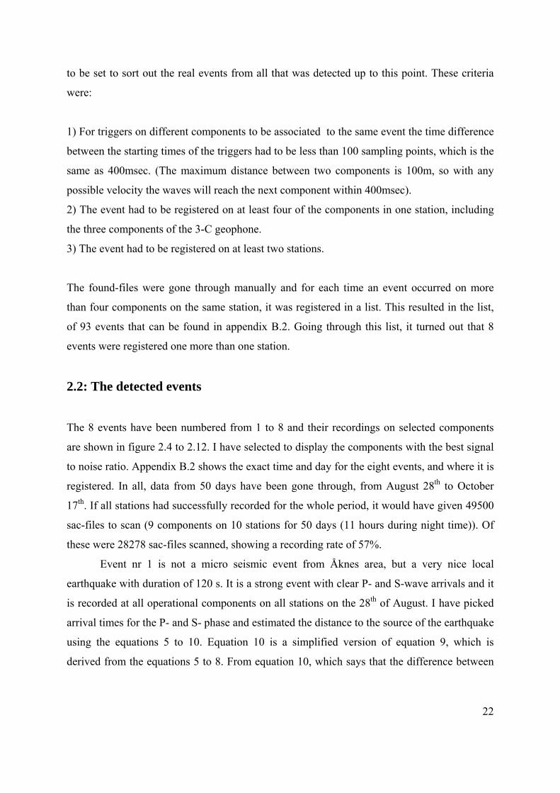
Event nr 1 is not a micro seismic event from Åknes area, but a very nice local

earthquake with duration of 120 s. It is a strong event with clear P- and S-wave arrivals and it

is recorded at all operational components on all stations on the 28th of August. I have picked

arrival times for the P- and S- phase and estimated the distance to the source of the earthquake

using the equations 5 to 10. Equation 10 is a simplified version of equation 9, which is

derived from the equations 5 to 8. From equation 10, which says that the difference between

22

the arrivaltimes of the p- and s-waves times 8 is equal to epicentral distance in km, I have

calculated the average epicentral distance from the stations to be 137km.

(Equation 5)

(Equation 6)

(Equation 7)

(Equation 8)

(Equation 9)

(Equation 10)

Where α is the p-wave velocity, β is the S-wave velocity, Tα is the traveltime for the p-wave

from the source to the geophone, Tβ is the traveltime for the s-wave from source to geophone,

Tαa is the arrivaltime for the p-wave, Tβa is the arrivaltime for the s-wave and T0 is the origin

time of the earthquake. The value 8 in equation 10 is what is regularly used for earth

continental crust. It was a bit difficult to pick accurate arrivaltimes, but I found that the event

was closest to the stations S1, S2 and S4, and furthest away from stations S6 and S7. This

indicates that the source is in a NE direction. A close-up of event nr 1 is given in figure 2.4.

3050 3100 3150 3200 3250

-5000

0

5000

Event nr. 1

seconds

ampl

itude

Figure 2.4: Event nr. 1 with a duration of 120 s. This is from the trace with best

signal to noise ratio, component S6-3 . Registered on all operational components

on all stations. This is a close-up of sac-file, recorded by component 2 at station S5,

with starting time:2005.08.28-25.59.59.

23

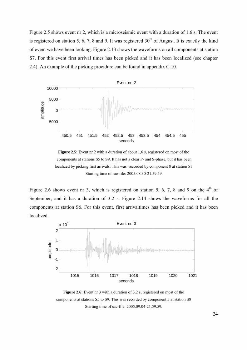
Figure 2.5 shows event nr 2, which is a microseismic event with a duration of 1.6 s. The event

is registered on station 5, 6, 7, 8 and 9. It was registered 30th of August. It is exactly the kind

of event we have been looking. Figure 2.13 shows the waveforms on all components at station

S7. For this event first arrival times has been picked and it has been localized (see chapter

2.4). An example of the picking procidure can be found in appendix C.10.

450.5 451 451.5 452 452.5 453 453.5 454 454.5 455

-5000

0

5000

10000Event nr. 2

seconds

ampl

itude

Figure 2.5: Event nr 2 with a duration of about 1,6 s, registered on most of the

components at stations S5 to S9. It has not a clear P- and S-phase, but it has been

localized by picking first arrivals. This was recorded by component 8 at station S7

Starting time of sac-file: 2005.08.30-21.59.59.

Figure 2.6 shows event nr 3, which is registered on station 5, 6, 7, 8 and 9 on the 4th of

September, and it has a duration of 3.2 s. Figure 2.14 shows the waveforms for all the

components at station S6. For this event, first arrivaltimes has been picked and it has been

localized.

1015 1016 1017 1018 1019 1020 1021

-2

-1

0

1

2x 104 Event nr. 3

seconds

ampl

itude

Figure 2.6: Event nr 3 with a duration of 3.2 s, registered on most of the

components at stations S5 to S9. This was recorded by component 5 at station S8

Starting time of sac-file: 2005.09.04-21.59.59.

24

Figure 2.7 shows event nr. 4, which is only registered on station 1 and 2 on September 5th. It

has a duration of 1.2 s. Figure 2.15 shows the waveforms for all the components at station S2.

This microseismic event has also been localized.

1517 1517.5 1518 1518.5 1519 1519.5 1520 1520.5

-1500

-1000

-500

Event nr. 4

seconds (3600 per hour)

ampl

itude

Figure 2.7 Event nr 4 with a duration of 1.2 s, registered on four components

at station S1 and all components at S2. This was recorded by component 5 at

station S2 Starting time of sac-file: 2005.09.05-02.59.59.

Figure 2.8 shows event nr 5, which is also registered on September 5th by station 1, 2 and 4. It

has a duration of 1.6 s. Figure 2.16 shows the waveforms from all the components at station

S2. This is a microseismic event, and it has been localized.

2282 2282.5 2283 2283.5 2284 2284.5 2285 2285.5

-3000

-2000

-1000

Event nr. 5

seconds

ampl

itude

Figure 2.8: Event nr 5 with a duration of 1.6 s, registered on most of the

components at stations S1, S2 and S4. This was recorded by component 0 at station S1

Starting time of sac-file: 2005.09.05-05.59.59.

Figure 2.9 shows event nr. 6, which is registered on station S1 and S6 the 10th of September.

It is a clear event with a high signal to noise ratio, with duration of about 30 s. But it has no

25

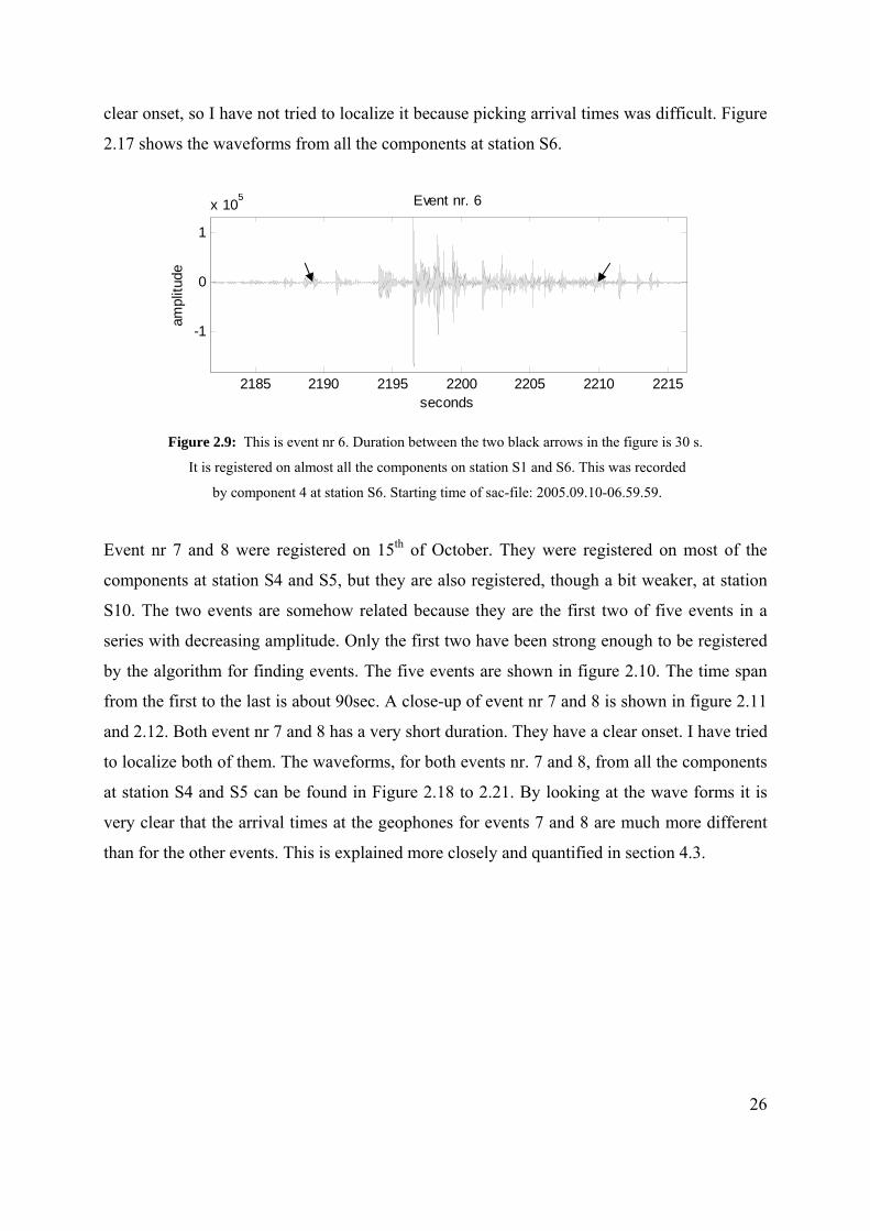
clear onset, so I have not tried to localize it because picking arrival times was difficult. Figure

2.17 shows the waveforms from all the components at station S6.

2185 2190 2195 2200 2205 2210 2215

-1

0

1

x 105 Event nr. 6

seconds

ampl

itude

Figure 2.9: This is event nr 6. Duration between the two black arrows in the figure is 30 s.

It is registered on almost all the components on station S1 and S6. This was recorded

by component 4 at station S6. Starting time of sac-file: 2005.09.10-06.59.59.

Event nr 7 and 8 were registered on 15th of October. They were registered on most of the

components at station S4 and S5, but they are also registered, though a bit weaker, at station

S10. The two events are somehow related because they are the first two of five events in a

series with decreasing amplitude. Only the first two have been strong enough to be registered

by the algorithm for finding events. The five events are shown in figure 2.10. The time span

from the first to the last is about 90sec. A close-up of event nr 7 and 8 is shown in figure 2.11

and 2.12. Both event nr 7 and 8 has a very short duration. They have a clear onset. I have tried

to localize both of them. The waveforms, for both events nr. 7 and 8, from all the components

at station S4 and S5 can be found in Figure 2.18 to 2.21. By looking at the wave forms it is

very clear that the arrival times at the geophones for events 7 and 8 are much more different

than for the other events. This is explained more closely and quantified in section 4.3.

26

2600 2650 2700 2750 2800 2850 2900

-2000

0

2000

4000

Events 7 and 8

seconds

ampl

itude

Figure 2.10: The five related events which occurs over a time-span of 90 s.

The first two are events nr 7 and nr 8. This has been registered on most of the

components at station S4 an S5, but also on some components at station S10.

This was recorded by component 4 at station S4 Starting time of sac-file:

2005.10.15-06.59.59.

2714 2714.22714.42714.62714.8 2715 2715.22715.42715.62715.8 2716

-2000

0

2000

4000

Event nr. 7

seconds

ampl

itude

Figure 2.11: Event nr 7, the first in a serie of five events. It has a duration of 0.8 s.

This is from the same file as figure 2.10 and 2.12.

2741.2 2741.4 2741.6 2741.8 2742 2742.2 2742.4 2742.6 2742.8

-1000

0

1000

2000

3000

4000

Event nr. 8

seconds

ampl

itude

Figure 2.12: Event nr 8, the second in a serie of five. The duration is about 0.8 s.

This is from the same file as figure 2.10 and 2.11.

27

seconds (in the figure: 451.5 s to 435.9 s)

Figure 2.13: Waveforms for event nr. 2, at all the components in station S7.

28

seconds (in the figure: 1014 s to 1020 s)

Figure 2.14: Event nr. 3. Waveforms from all the components at station S6

29

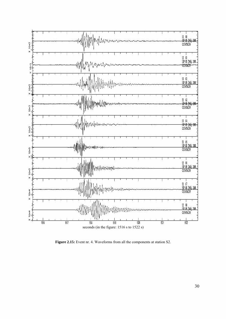
seconds (in the figure: 1516 s to 1522 s)

Figure 2.15: Event nr. 4. Waveforms from all the components at station S2.

30

seconds (in the figure: 2281 s to 2287 s)

Figure 2.16: Events nr. 5. Waveforms from all the components at station S2.

31

seconds (in the figure: 0 to 85 s)

Figure 2.17: Event nr. 6. Waveforms from all the components at station S6.

32

seconds (in the figure: 2712.5 s to 2717 s)

Figure 2.18: Event nr. 7. Waveforms from all the comopnents at station S4.

33

seconds (in the figure: 2740 s to 2743 s)

Figure 2.19: Event nr. 8. Waveforms from all the components at station S4.

34

seconds (in the figure: 2712 s to 2715 s)

Figure 2.20: Event nr. 7. Waveforms from all the components at station S5.

35

seconds (in the figure: 2739 s to 2742 s)

Figure 2.21: Event nr. 8. Waveforms from all the components at station S5.

36

3: VELOCITY MODEL

3.1: Travel time-distance plot from dynamite blasts

We are interested in finding positions of seismic events or the distance from receiver to

source. All the information we have is the arrivaltimes at geophones at the surface. What we

need is a relation between the epicentral distances and the traveltimes. This is traditionaly

obtained by building a velocity model and calculating the traveltimes in this model. But there

is another option: if we have recorded signals from a source with known position and origin

time, both traveltimes and distances from that source can be calculated. A plot of traveltimes

versus distances to the source provides us with the relationship between these two parameters,

which we need for localizing other sources.

During the last two recording days (16th

and 17th of October) of the temporary

passive seismic IHR network (with

which I have been working), a seismic

refraction survey was done. The

location of the line of receivers is shown

in figure 3.1. Five dynamite blasts were

used as a source in the refraction survey.

The times and the positions of these

blasts are known, and they were all

recorded very clearly on all operational

geophones at all stations in the IHR

network (which more or less covers the

whole slide area). The positions of the

five blasts are shown in figure 1.6 and 4.4, where they are marked SP1 to SP5 in blue. SP is

short for Shot Point. Appendix B.3 gives their coordinates and time. By using the information

on the five shots together with arrivaltimes picked at the geophones, I have calculated

traveltimes and plotted them together with their corresponding source-receiver distances in a

37

distance-traveltime plot. This gives an average relation between traveltimes and epicentral

distance throughout the area.

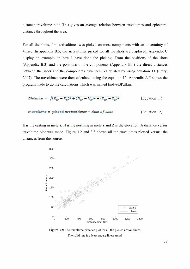
For all the shots, first arrivaltimes was picked on most components with an uncertainty of

4msec. In appendix B.5, the arrivaltimes picked for all the shots are displayed. Appendix C

display an example on how I have done the picking. From the positions of the shots

(Appendix B.3) and the positions of the components (Appendix B.4) the direct distances

between the shots and the components have been calculated by using equation 11 (Frery,

2007). The traveltimes were then calculated using the equation 12. Appendix A.5 shows the

program made to do the calculations which was named findvelSPall.m.

(Equation 11)

(Equation 12)

E is the easting in meters, N is the northing in meters and Z is the elevation. A distance versus

traveltime plot was made. Figure 3.2 and 3.3 shows all the traveltimes plotted versus. the

distances from the source.

0 200 400 600 800 1000 1200 14000

50

100

150

200

250

300

350

distance from SP

trave

ltim

e m

s

data 1 linear

Figure 3.2: The traveltime-distance plot for all the picked arrival times.

The solid line is a least square linear trend.

38

0 200 400 600 800 1000 1200 14000

50

100

150

200

250

300

350

distance from SP

trave

ltim

e m

s

v1v2v3v4v5

Figure 3.3: Traveltime-distance plot for all the picked arrival times.

The different colours represent arrival times for the five shots,

v1 is for SP1, v2 is for SP2 and so on.

Figure 3.3 shows the travel times in the traveltime-distance plot with traveltimes for each of

the shots plotted with different colours, labelled from v1 to v5 (for the shots SP1 to SP5

respectively). The plot shows that all the arrivaltimes fall on the same trend within a certain

range, except for some outliers from SP1 and SP3. The outliers could result from bad picking.

I have chosen to use a linear trend calculated from all the traveltimes together to find the

relation between traveltime and epicentral distance. The linear trend in figure 3.2 is found

automatically in Matlab by a least-squares method. The slope of the traveltime-distance curve

(also called t-x diagram) corresponds to the slowness of the waves (Musset & Khan, 2000).

The trend in figure 3.2 follows equation 13.

Traveltime = (slowness X distance) + Tintercept (Equation 13)

39

The slowness is 0.19 ms/m and the Tintercept is 43.737 ms. Equation 13 with the values of

Tintercept and slowness gives a relation between epicentral distances and traveltimes, which was

what I wanted to find. The equation will be used in the localization process in chapter 4.

3.2: The velocity model

From the relation between traveltimes and epicentral distance a velocity model can be

derived. Given the slowness equal to 0.19 we can find the velocity with equation 14.

(Equation 14)

The linear trend in figure 3.2 does not intersect the time axis at zero. A timing error of the

shots can cause a Tintercept larger than zero if the real time of the shot has been delayed. Also if

I have in general picked all the arrivaltimes later than when they actually arrived, the whole

trend will move upwards in the t-x diagram, causing Tintercept to be larger than zero. If the

timing and picking are correct a Tintercept larger than zero indicates the presence of a low

velocity zone over a half space with a uniform velocity. In a t-x diagram, the direct wave

following the surface will result in a line with a steep slope, starting at the origin and

intersecting the next first arrival line. The slope of this line gives the slowness of the first

layer; this together with Tintercept can give the thickness of the surface layer (Musset & Khan,

2000). In the plot in figure 3.2 it is not possible to draw such a line from the plotted values so

it is not possible to say how thick the first layer is or the velocity. It could be that none of the

distances between shot point and component are short enough for the direct wave from the

shot to arrive first. From this interpretation and the velocity found in equation 14 I can deduce

that the velocity model is of the form shown in figure figure 3.4.

Figure 3.4: The velocity. The white layer on top is thin, but the velocity

and thickness is unknown. The grey layer has a uniform velocity of 5.26 km/s

40

There is a thin layer at the surface with unknown velocity and unknown thickness. Below the

surface layer there is a uniform half space with velocity of 5.26 km/s. I know that the whole

area consists of gneiss, which probably corresponds to the uniform half space with velocity

5.26 km/s. The thin surface layer could be gneiss that are heavily fractured, and thus have a

low velocity. If some of the events found are so close to a component that the waves which

travel through the surface layer arrives first, the result of the localization using this model can

be a bit inaccurate.

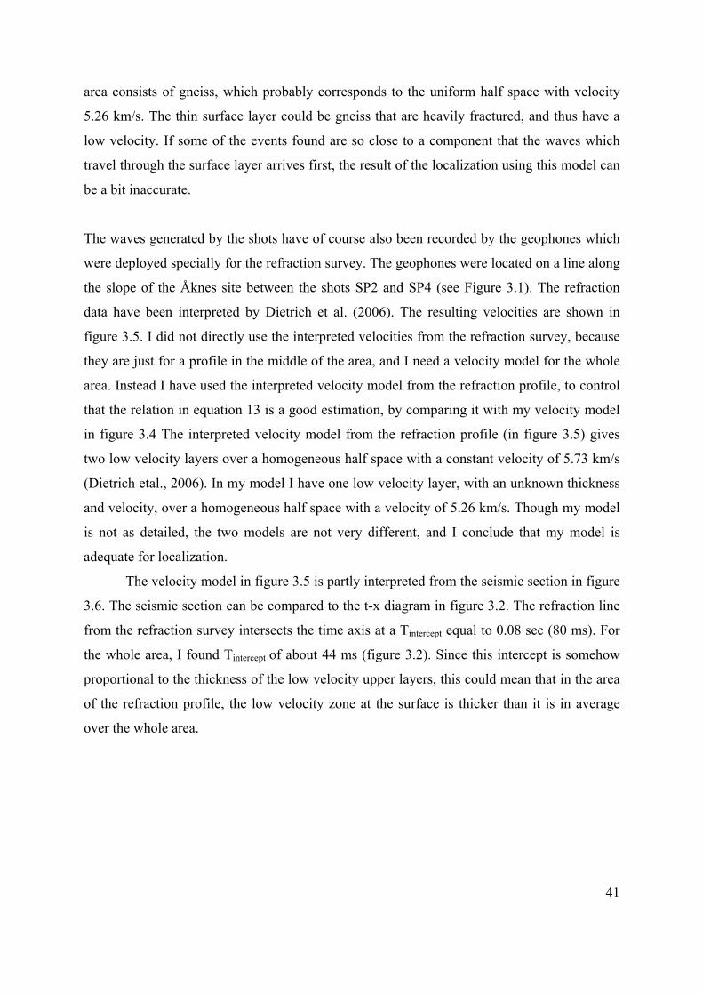
The waves generated by the shots have of course also been recorded by the geophones which

were deployed specially for the refraction survey. The geophones were located on a line along

the slope of the Åknes site between the shots SP2 and SP4 (see Figure 3.1). The refraction

data have been interpreted by Dietrich et al. (2006). The resulting velocities are shown in

figure 3.5. I did not directly use the interpreted velocities from the refraction survey, because

they are just for a profile in the middle of the area, and I need a velocity model for the whole

area. Instead I have used the interpreted velocity model from the refraction profile, to control

that the relation in equation 13 is a good estimation, by comparing it with my velocity model

in figure 3.4 The interpreted velocity model from the refraction profile (in figure 3.5) gives

two low velocity layers over a homogeneous half space with a constant velocity of 5.73 km/s

(Dietrich etal., 2006). In my model I have one low velocity layer, with an unknown thickness

and velocity, over a homogeneous half space with a velocity of 5.26 km/s. Though my model

is not as detailed, the two models are not very different, and I conclude that my model is

adequate for localization.

The velocity model in figure 3.5 is partly interpreted from the seismic section in figure

3.6. The seismic section can be compared to the t-x diagram in figure 3.2. The refraction line

from the refraction survey intersects the time axis at a Tintercept equal to 0.08 sec (80 ms). For

the whole area, I found Tintercept of about 44 ms (figure 3.2). Since this intercept is somehow

proportional to the thickness of the low velocity upper layers, this could mean that in the area

of the refraction profile, the low velocity zone at the surface is thicker than it is in average

over the whole area.

41

Figure 3.5: A vertical cut from the refraction profile. y-axis are elevation in meters and x-axis are horizontal

distance from the starting point of the profile. In the white box are the interpreted velocities in three different

layers. The yellow letters form A to E represents interpretation from the shots SP1 to SP5. The points B C, and D

marked in red, are the end points of the shots SP2, SP3 and SP4. The white dots at the surface marks the

receivers (Dietrich etal., 2006).

Figure 3.6: Seismic section from SP2 recorded in the refraction survey. This is some of the background from

which the velocity model in figure 3.6 had been interpreted. Refraction line from the homogenous half space I

have traced out with a solid line. (modified from Dietrich etal., 2006.)

42

What is shown in this paragraph is not important for the results of my work, but I have chosen

to include it to show that different approaches have been tried out. I tested also the possibility

of using a model with a velocity that varies linearly with depth. Figure 3.7 shows in different

colours the calculated distances versus traveltimes for five different gradients, varying from

0.0625 km/s to 0.1 km/s. For each gradient three different values of 0.5 km/s, 1.25 km/s and 2

km/s were also tested for the surface velocity. When comparing figure 3.7 with figure 3.2

showing the measured results, we see that none of the trends here fit the data. The traveltimes

plotted in figure 3.3 should have fallen on one of the trends in figure 3.7 if a velocity model

with a gradient would have been adequate. The conclusion is that a velocity model with a

velocity that vary linearly with depth is not a good model and that a slow layer above a

homogeneous half space is much more adequate.

Figure 3.7: Traveltime vs. distance plot. The different colours correspond to different gradients, labelled “gr” in

the legends. The three trends with the same colour have different surface velocity, labelled “svel” in the legend.

3.3: Uncertainty concerning the locations of the geophones

In the sac-files containing the data, the components are numbered from 0 to 8, and there is no

information in the header on the location of the geophones, and no info on which of the nine

components at a station is part of a 3-C geophone. The stations are in the data named S1 to

S10. The information I have on the positions of the geophones is the same as used by Frery

(2007). In this information the stations are labelled the same way, S1 to S10, as in the data,

but the components are labelled 1 to 7 and the 3-C geophone is one of these 7 components

(which one changes from station to station). I had therefore to identify which of my data files 43

belong to which component in Frery’s table. In order to do that I compared the waveforms of

the shots SP1 to SP5 in my data to those plotted by Frery in her report. The correspondence

between the two numbering systems can be found in appendix B.5.

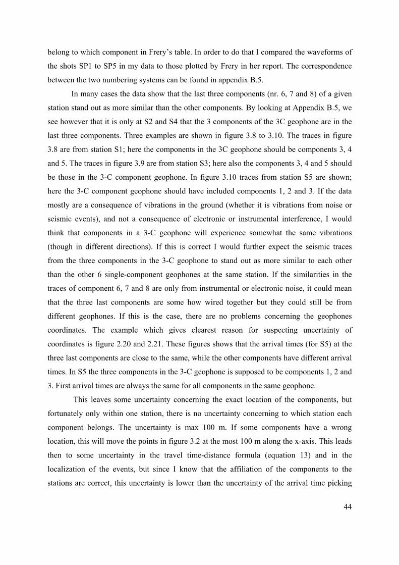
In many cases the data show that the last three components (nr. 6, 7 and 8) of a given

station stand out as more similar than the other components. By looking at Appendix B.5, we

see however that it is only at S2 and S4 that the 3 components of the 3C geophone are in the

last three components. Three examples are shown in figure 3.8 to 3.10. The traces in figure

3.8 are from station S1; here the components in the 3C geophone should be components 3, 4

and 5. The traces in figure 3.9 are from station S3; here also the components 3, 4 and 5 should

be those in the 3-C component geophone. In figure 3.10 traces from station S5 are shown;

here the 3-C component geophone should have included components 1, 2 and 3. If the data

mostly are a consequence of vibrations in the ground (whether it is vibrations from noise or

seismic events), and not a consequence of electronic or instrumental interference, I would

think that components in a 3-C geophone will experience somewhat the same vibrations

(though in different directions). If this is correct I would further expect the seismic traces

from the three components in the 3-C geophone to stand out as more similar to each other

than the other 6 single-component geophones at the same station. If the similarities in the

traces of component 6, 7 and 8 are only from instrumental or electronic noise, it could mean

that the three last components are some how wired together but they could still be from

different geophones. If this is the case, there are no problems concerning the geophones

coordinates. The example which gives clearest reason for suspecting uncertainty of

coordinates is figure 2.20 and 2.21. These figures shows that the arrival times (for S5) at the

three last components are close to the same, while the other components have different arrival

times. In S5 the three components in the 3-C geophone is supposed to be components 1, 2 and

3. First arrival times are always the same for all components in the same geophone.

This leaves some uncertainty concerning the exact location of the components, but

fortunately only within one station, there is no uncertainty concerning to which station each

component belongs. The uncertainty is max 100 m. If some components have a wrong

location, this will move the points in figure 3.2 at the most 100 m along the x-axis. This leads

then to some uncertainty in the travel time-distance formula (equation 13) and in the

localization of the events, but since I know that the affiliation of the components to the

stations are correct, this uncertainty is lower than the uncertainty of the arrival time picking

44

and the uncertainty of the method for making the velocity model itself. So the work on this

thesis is not all a waste even if the positions turn out to be a bit wrong within a station. .

Figure 3.8: Traces from all the components at station S1. Components 3, 4 and 5 should comprise the 3C geophone. This is recorded on September 10th. The starting time of the sac-file is 22.59.59.

45

Figure 3.9: Traces from all the components at station S3. Components 3, 4 and 5 should be from the 3C geophone. This is recorded on August 26th. Starting time of the sac-file is 10.59.58.

46

Figure 3.10: Traces from all the components at station S5. Components 1, 2 and 3 should be from the 3C geophone. This is recorded on August 28th. Starting time of sac-file is 02.59.59.

47

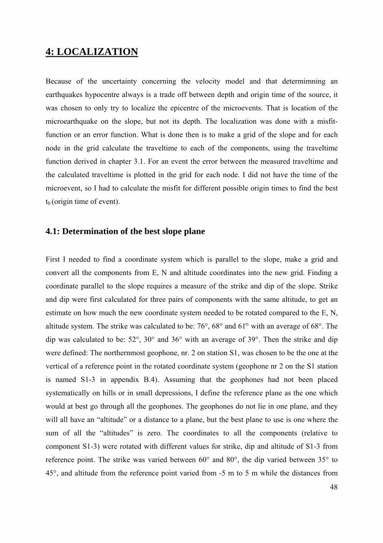
4: LOCALIZATION

Because of the uncertainty concerning the velocity model and that determimning an

earthquakes hypocentre always is a trade off between depth and origin time of the source, it

was chosen to only try to localize the epicentre of the microevents. That is location of the

microearthquake on the slope, but not its depth. The localization was done with a misfit-

function or an error function. What is done then is to make a grid of the slope and for each

node in the grid calculate the traveltime to each of the components, using the traveltime

function derived in chapter 3.1. For an event the error between the measured traveltime and

the calculated traveltime is plotted in the grid for each node. I did not have the time of the

microevent, so I had to calculate the misfit for different possible origin times to find the best

t0 (origin time of event).

4.1: Determination of the best slope plane

First I needed to find a coordinate system which is parallel to the slope, make a grid and

convert all the components from E, N and altitude coordinates into the new grid. Finding a

coordinate parallel to the slope requires a measure of the strike and dip of the slope. Strike

and dip were first calculated for three pairs of components with the same altitude, to get an

estimate on how much the new coordinate system needed to be rotated compared to the E, N,

altitude system. The strike was calculated to be: 76°, 68° and 61۫° with an average of 68°. The

dip was calculated to be: 52°, 30° and 36° with an average of 39°. Then the strike and dip

were defined: The northernmost geophone, nr. 2 on station S1, was chosen to be the one at the

vertical of a reference point in the rotated coordinate system (geophone nr 2 on the S1 station

is named S1-3 in appendix B.4). Assuming that the geophones had not been placed

systematically on hills or in small depressions, I define the reference plane as the one which

would at best go through all the geophones. The geophones do not lie in one plane, and they

will all have an “altitude” or a distance to a plane, but the best plane to use is one where the

sum of all the “altitudes” is zero. The coordinates to all the components (relative to

component S1-3) were rotated with different values for strike, dip and altitude of S1-3 from

reference point. The strike was varied between 60° and 80°, the dip varied between 35° to

45°, and altitude from the reference point varied from -5 m to 5 m while the distances from

48

Strike = 72°

Dip = 35.9°

Distance from reference point = 4 m

The standard deviation was most sensitive to the value of dip.

4.2: Method for localization

The next step was to use the best slope plane and write an algorithm for localizing the

microearthquakes on this plane. The program, lokalisering.m, that was written for the

localization can be found in Appendix A.6. The first thing the program does is to rotate the

coordinates of the geophones from East, North and altitude, according to the strike and dip

with rotational matrixes shown in equation 16 and 17.

(Equation 15)

(Equation 16)

Where X’, Y’ and Z’ are the new coordinates rotated horizontally according to the strike, α,

and X, Y and Z are the new coordinates rotated according to dip, β. The cell size in the grid is

20 m x 20 m. The distance along slope (omitting z) between the geophone and a node in the

grid is then calculated using equation 18.

(Equation 17)

49

Where index n indicates node and c indicates geophone. The theoretical traveltime from that

node to the geophone can then be calculated by using equation 19. Which is the relation found

in section 3.1.

(Equation 18)

Were Tintercept is the intersection point between traveltime curve and traveltime axis in the

traveltime-distance plot. Tintercept = 44 ms, slowness = 0.19 ms/m. I have picked the arrival

times at the different components but in order to calculate the measured traveltimes, I need to

calculate the origin time t0 of the microevent. This is done by using equation 20.

(Equation 19)

In order to evaluate it, I calculate misfit functions with different values for t0, varying from 0

to 120ms before the first arrival. Finally the misfits from all components at each node are

summed up. The misfits are calculated by using equation 21.

(Equation 20)

50

The misfit is plotted with a contour plot. The nodes with the lowest misfit are thought to be

the location of the microevent. The calculations in equations 18 to 21 was tested for different

values of t0 and plotted. To learn how the algorithm behaves, this was tested out on the five

active shots, SP1 to SP5, because here we know the exact location and time. Figure 4.1 to 4.3

shows the result of the localization of SP2 using three different values for t0. I have also

plotted the locations of the stations S1 to S10 but omitted their numbers for clarity of the

figure. The locations of the five shots SP1 to SP5 are plotted in red stars. The values of the

contour circles are only important for the inner circles to be able to compare between different

values of t0. It is not possible to read the values of the highest misfit contours, but they are not

important for the localization. For station number of the stations see figure 4.4 (or 1.6) and

notice that the misfit plots are somehow rotated 90 degrees compared to figure 4.4. We know

that the t0 is 12.52.00.004 and that SP2 is located in the middle of the area just above station

S7. The minimum misfit corresponds well to the position of the three values of t0. Figure 4.2

for which t0 is closest to the real t0 of the shot, has the largest area around the location with the

lowest misfit values. The conclusion is that the misfit function can be used even if the

microevents are not known. The form of the misfit function can give information on it also.

Testing the five shots shows that the localization method works well. Since it was successful

to locate the five shots I also concluded that the velocity model is not too bad.

2.58e+0045.15e+004

7.73e+004

1.03e+005

1.29e+005

1.55e+005

1.8e+005

2.06e+005

2.32e+0052.58e+005 2.58e+0052.83e+005

2.83e+0053.09e+005 3.09e+0053.35e+005 3.35e+0053.61e+005

3.61e+0053.87e+005 3.87e+0054.12e+005 4.12e+005

4.38e+005 4.38e+0054.64e+005 4.64e+0054.9e+005

4.9e+0055.15e+005 5.15e+0055.41e+005

5.41e+005.67e+005 5.67e+05.93e+005

5.93e+0056.19e+005 6.19e+006.44e+005 6.44e+006.7e+005

6.7e+006.96e+005

6.96e+

7.22e+005 7.22e+

7.47e+005 7.47e7.73e+005 7.73e7.99e+005 7.99e8.25e+005

8.25

8.5e+005 8.58.76e+005 8.79.02e+005

9.02

9

9.28e+005

9.2

9.

9.54e+005

9.

9.5

9.79e+005

9.79e+005

9

9.7

1.01e+006

1.01e+006

1.0

1

1.03e+006

1.03e+006

1

1.

1.06e+006

1.06e+006

1

1.

1.08e+006

1.08e+006

1

1

1.11e+006

1.11e+006

1

1

1.13e+006

11.16e+006

1

1.19e+006

1.19e+0061.21e+0061.24e+0061.26e+006

Down slope in m

Alo

ng s

trike

in m

Lokalization of SP2, t zero = 12.52.00.023

-400 -200 0 200 400 600 800 1000 1200 1400-500

-400

-300

-200

-100

0

100

200

300

400

500

Figure 4.1: Localization of SP2, localized using t0 = 12.52.00.023. The location of the

geophones are marked with magenta circles, the locations of SP1 to SP5 are marked with red stars.

51

2.58e+004

5.15e+004

7.73e+004

1.03e+005

1.29e+005

1.55e 005

1.8e+005 1.8e+0052.06e+005

2.06e+0052.32e+005 2.32e+0052.58e+005 2.58e+005

2.83e+005 2.83e+0053.09e+005 3.09e+0053.35e+005 3.35e+005

3.61e+005 3.61e+0053.87e+005 3.87e+0054.12e+005

4.12e+0054.38e+005 4.38e+0054.64e+005 4.64e+004.9e+005 4.9e+0055.15e+005 5.15e+005.41e+005

5.41e+5.67e+005 5.67e5.93e+005 5.936.19e+005

6.196.44e+005 6.46.7e+005

6.6.96e+005

6

7.22e+005 7

7.47e 005

7

7.73e+005 7.73e

7

7.99e+005

7

8.25e+005 8

8.

8.5e+005

8.5e+005

8.5

8

8.76e+005

8

9.02e+005

9

9.28e+005

9.28e+005 9

9.54e+005

9.54e+005 99.79e+0051.01e+0061.03e+0061.06e+006

Down slope in m

Alo

ng s

trike

in m

Lokalization of SP2, t zero = 12.52.00.008

-400 -200 0 200 400 600 800 1000 1200 1400-500

-400

-300

-200

-100

0

100

200

300

400

500

Figure 4.2: this is localization of SP2, localized wit t0 = 12.52.00.008. The magenta

circles are the location of the geophones, SP1 to SP2 are marked with red stars.

2.58e+004

5.15e+004

7.73e+0041.03e+005

1.29e+005 1.29e+005

1.55e+005 1.55e+0051.8e+005 1.8e+0052.06e+005 2.06e+005

2.32e+005 2.32e+0052.58e+005 2.58e+0052.83e+005

2.83e+0053.09e+005 3.09e+0053.35e+005 3.35e+0053.61e+005 3.61e+0053.87e+005 3.87e+0054.12e+005

4.12e+04.38e+005

4.38e+

4.64e+005 4.64e4.9e+005

4.9e+05.15e+005 5.15e5.41e+005 5.41e

5.67e+0055

5.93e+0055

6.19e+005

6.1

6

6.44e+005

6

6.46.7e+005

6.7e+005

6.7

6

6.96e+005

6.96e+005

6.

67.22e+005

7.22e+0057

77.47e+005

7.47e+005

7

7

7.73e+005

7.73e+0057

7.99e+005

7.99e+0057

8.25e+0058.5e+0058.76e+005

Down slope in m

Alo

ng s

trike

in m

Lokalization of SP2, t zero = 12.51.59.993

-400 -200 0 200 400 600 800 1000 1200 1400-500

-400

-300

-200

-100

0

100

200

300

400

500

Figure 4.3: This is SP2 localized with t0 = 12.51.59.993. The magenta circles are the

location of the geophones, the red stars are the location of the shots SP1 to SP5. 52

4.3: Results from the localization of microevents

I have only tried to localize events nr. 2, 3, 4, 5, 7 and 8. Event nr.1 has not been tried

localized because it is an earthquake with a distance of 137km to the site. Event nr. 6 has not

been tried localized either, because it had no clear onset and the first arrival times could not

be picked. Six micrevents have been identified and successfully localized. Figure 4.5 to 4.8

shows the results.

The misfit function of event nr 2 is plotted in figure nr 4.5. This event appears to be

located at the same altitude as S10 but just outside the instable area, on the other side of the

crevasse limiting the area eastward.

The misfit function of event nr 3 is plotted in figure 4.6. This is a microseismic event

with origin in the lower eastern part of the instable area, about in the middle between S10 and

S8.

The misfit function of event nr 4 is plotted in figure 4.7. The event appears to be

located in the open fracture at the top of the area just between S1 and S2.

Event nr. 5 is also appears to located by the open fracture close the stations S1, S2 and

S3.

Within a range of plus/minus 20 ms, the plots of the misfit does not vary very much

with t0 but going outside this range the plot changes. The location of the lowest misfit value

does vary much with the slowness. Within a range of plus/minus 0.05 ms/m the position of

minimum misfit value moves about 200 m (when the velocity changes from 4 km/s to 6.7

km/s). If the Tintercept changes with plus/minus 40 ms the position of minimum misfit value

changes 100 m in opposite directions. Within a range of plus/minus 10 ms sec the position of

minimum misfit value changes less than 20 meters. Overall the success of the localization

depends on having good values for Tintercept and the slowness. This also confirms that the

relation in equation 13 and 19 is a good estimation for the slope (since the localization of SP1

to SP5 was successful).

53

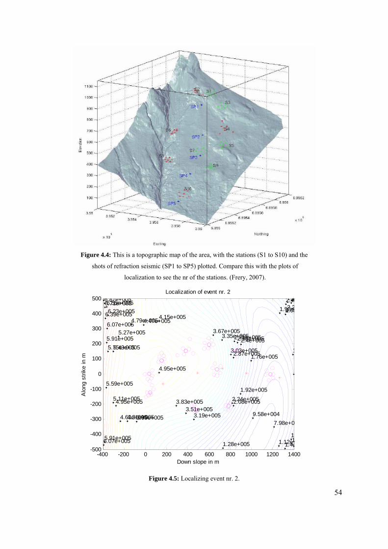
Figure 4.4: This is a topographic map of the area, with the stations (S1 to S10) and the

shots of refraction seismic (SP1 to SP5) plotted. Compare this with the plots of

localization to see the nr of the stations. (Frery, 2007).

7.98e+09.58e+004

1.12e+1.28e+005

1

1.44

1

1

1.76e+005

1

1.92e+005

1.92e+

1

2.08e+005

2.08

2.24e+005

2.2

2.4e+005

2.4e

2.56e+005

2.5

2.71e+005

2

2.87e+0053.03e+005

3.19e+005

3.35e+005

3.51e+005

3.67e+005

3.83e+005

3.99e+005

4.15e+005

4.31e+005

4.47e+005

4.63e+005

4.79e+005

4.95e+005

4.95e+005

5.11e+005

5.27e+005

5.43e+005

5.59e+005

5.75e+005

5.91e+005

5.91e+005

6.07e+005

6.07e+005

6.23e+0056.39e+005

6.55e+0056.71e+0056.87e+005

Down slope in m

Alo

ng s

trike

in m

Localization of event nr. 2

-400 -200 0 200 400 600 800 1000 1200 1400-500

-400

-300

-200

-100

0

100

200

300

400

500

Figure 4.5: Localizing event nr. 2.

54

1.85e+004

3.7e+004

5.56e+004

7.41e+0

9.26e+0041.11e

1.3e+005 1.

1.48e+005 11.67e+005

1.67e

1.6

1.85e+005

1

1.8

2.04e+005

2.04e+

2

2.22e+005

2.2

2

2.41e+005

2.41

2

2.59e+0052.78e+005

2.96e+005

2

3.15e+0053.33e+005

3.52e+005

3.7e+0053.89e+005

4.07e+0054.26e+0054.45e+005

4.63e+005

4.82e+005

5e+005

5.19e+005

5.37e+005

5.56e+005

5.74e+005

5.93e+005

6.11e+005

6.3e+005

6.48e+005

6.48e+005

6.67e+005

6.67e+005

6.85e+005

6.85e+005

7.04e+005

7.04e+005

7.22e+005

7.22e+005

7.41e+005

7.41e+005

7.78e+0057.96e+005

Down slope in m

Alo

ng s

trike

in m

Localization of event nr. 3

-400 -200 0 200 400 600 800 1000 1200 1400-500

-400

-300

-200

-100

0

100

200

300

400

500

Figure 4.6: Localization of event nr 3.

1.63e+004

1.63e+0042.45e+004

3.26e+004

3.26e+004

4.08e+004

4.89e+004

5.71e+004

6.52e+004

6.52e+004

6.52e+004

7.34e+004

7.34e+004

8.16e+004

8.97e+004

9.79e+004

1.06e+005

1.14e+005

1.22e+005

1.3e+005

1.39e+005

1.47e+005

1.55e+005

1.63e+0051.71e+005

1.79e+005

1.88e+00

1.96e+005

2.04e+0

2.12e+0

2.2e+02.28e2.37e2.45

2.53e+0

2.62.622

2.9

2

3.02

3

3.1

3

3.

3

3

3

333

Down slope in m

Alo

ng s

trike

in m

Localization of event nr. 4

-400 -200 0 200 400 600 800 1000 1200 1400-500

-400

-300

-200

-100

0

100

200

300

400

500

Figure 4.7: Localization of event nr 4.

55

Figure 4.8: Localization of event nr 5.

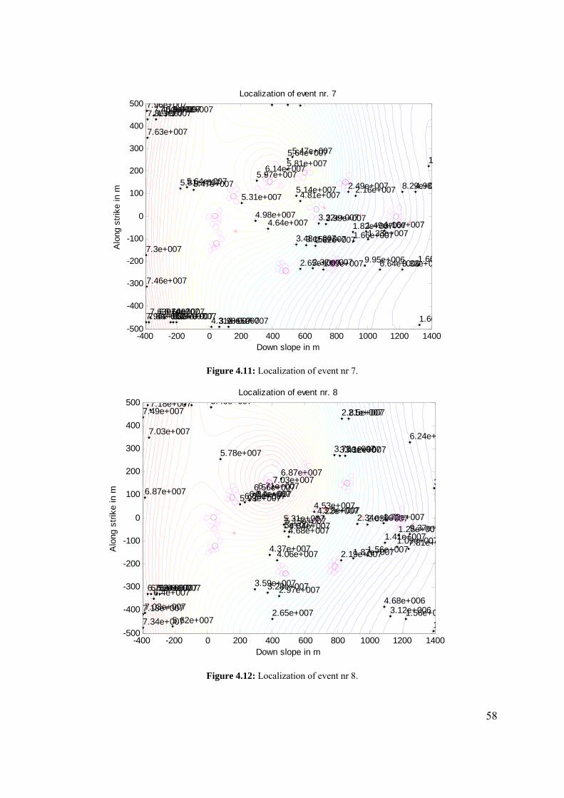
Events nr 7 and 8 are the first two in a series of four events, that are recorded over a time-span

of 80sec and they have a very short duration (0.8sec). The events have been recorded on

stations S4, S5 and S10, which were the only ones recording at that time. The result of the

localization of events nr. 7 and 8 shows highest misfit values within the area, and decreasing

misfit further away. From figure 2.18 and 2.19 that the biggest difference in arrivaltimes for

two components at the same station, for both event 7 and 8, is about 400 ms. The largest

distance possible between two components at one station is 100 m. If a seismic wave should

have traveled maximum 100 m in 400 ms it would have had a maximum velocity of 0.25

km/s. A velocity that low does not fit with the relation in equation 3.13 and 3.19. I therefore

tried to change the Tintercept, t0 and the slowness and found that the lowest value of misfit was

obtained with Tintercept equal to 0, a slowness equal to 2.39 ms/ms, and a t0 equal to 742 ms.

Figure 4.11 and 4.12 shows the localization of events 7 and 8. This result still has high misfit

values around the S4 and S5, but now it implies that the source is in a SSE direction.

56

2.42.5e+007

22.57e+007

2.57e+0072.65e+007 2.65e+007

2.72e+0072.79e+007

2.86e+007

2.93e+007

3e+007

Down slope in m

Alo

ng s

trike

in m

Localization of events nr. 7

-400 -200 0 200 400 600 800 1000 1200 1400-500

-400

-300

-200

-100

0

100

200

300

400

500

Figure 4.9: Localization of event nr. 7

3.01e

3.1e+007

3

3.1

3.19e+007 3.19e+007

3.27e+007 3.27e+007

3.36e+007

3.45e+0073.62e+007

3.7e+007

Down slope in m

Alo

ng s

trike

in m

Localization of event nr. 8

-400 -200 0 200 400 600 800 1000 1200 1400-500

-400

-300

-200

-100

0

100

200

300

400

500

Figure 4.10: Localization of event nr. 8

57

1.66

1.66

1

3.32e+0

4.98e

6.64e+006

8.29e+0

9.95e+006

1.16e+0071.33e+0071.49e+007

1.66e+0071.82e+007

1.99e+007

2.16e+007

2.32e+007

2.49e+007

2.65e+007

2.82e+007

2.99e+007

3.15e+007

3.32e+007

3.48e+007

3.65e+0073.98e+0074.31e+007

4.64e+007

4.81e+007

4.98e+007

5.14e+0075.31e+007

5.47e+007

5.47e+007

5.64e+007

5.64e+007

5.81e+007

5.81e+007

5.97e+007

5.97e+007

6.14e+007

6.14e+007

6.3e+007

6.47e+007

6.64e+007

6.8e+007

6.97e+007

7.13e+007

7.3e+007

7.3e+007

7.46e+007

7.46e+007

7.63e+007

7.63e+007

7.8e+007

7.8e+007

7.96e+007

7.96e+007

Down slope in m

Alo

ng s

trike

in m

Localization of event nr. 7

-400 -200 0 200 400 600 800 1000 1200 1400-500

-400

-300

-200

-100

0

100

200

300

400

500

Figure 4.11: Localization of event nr 7.

1.56e+01

3.12e+006

3

4.68e+006

6.24e+

7.81e+0

9.37e+1.09e+0071.25e+007

1.41e+0071.56e+007

1.72e+007

1.87e+007

2.03e+007

2.19e+007

2.34e+007

2.5e+007

2.65e+007

2.81e+007

2.97e+007

3.12e+007

3.28e+007

3.43e+007

3.59e+007

3.75e+007

3.9e+007

4.06e+007

4.22e+007

4.37e+007

4.53e+007

4.68e+0074.84e+0075e+0075.15e+0075.31e+007

5.46e+007

5.62e+007

5.78e+007

5.93e+007

6.09e+007

6.09e+007

6.24e+007

6.24e+007

6.4e+007

6.4e+007

6.56e+007

6.56e+007

6.71e+007

6.71e+0076.87e+007

6.87e+007

7.03e+007

7.03e+007

7.03e+007

7.18e+007

7.18e+007

7.34e+007

7.49e+007

Down slope in m

Alo

ng s

trike

in m

Localization of event nr. 8

-400 -200 0 200 400 600 800 1000 1200 1400-500

-400

-300

-200

-100

0

100

200

300

400

500

Figure 4.12: Localization of event nr 8.

58

5: DISCUSSION

From December 2005 to June 2006 an average of 8 to 10 events with durations under 8sec

were recorded per day on the permanent seismic network (Delarue, 2006). I have found 6

events with durations under 8sec in 50 days. Taken into account that I have only analyzed half

of the data, I have found about one event every fourth day. So I have found far less events

than what is detected on the permanent network. Some of the reasons for this could be that,

compared to the permanent seismic network, the stations in the temporary IHR network are

spaced further apart from each other. And if most of the microseismic events are too weak to

be registered on more than one station they will not be registered by my method. The fact that

many of the stations were not operative towards the end of the recording period of the IHR

system makes it even less possible for a weak event to be detected on more than one station.

It would have been interesting to look at some of the events that were recorded at all

the components on one station, but not on more than one station. Because these events could

be nice microseismic events perfect for localization, but not registered on more than one

station for the reason explained above. Though they will be difficult to localize, one could say

in which region of the slope the event comes from and thus say something about the seismic

activity of the slope.

The accuracy of the localization process depends on the accuracy of the arrival time-

picking and on how well the velocities have been modeled. If you have perfect velocities and

perfect first arrival picks, you can do prefect localization. But for doing that you need a much

more advanced localization method than I have used. One method one can use is ray tracing.

With a better velocity model one could maybe have found the hypocenter of the found events

nr.2, 3, 4 and 5 by using ray tracing.

The topography is not taken into account, for either the velocity modeling or the

localization. So for a better velocity model it would have also been necessary to take into

account the topography to be able to localize hypocenters.

There is a lot of noise in the data from field work and helicopter activity. Maybe the

performance of the system would have been better if the area had been free for activities in

the recording period.

59

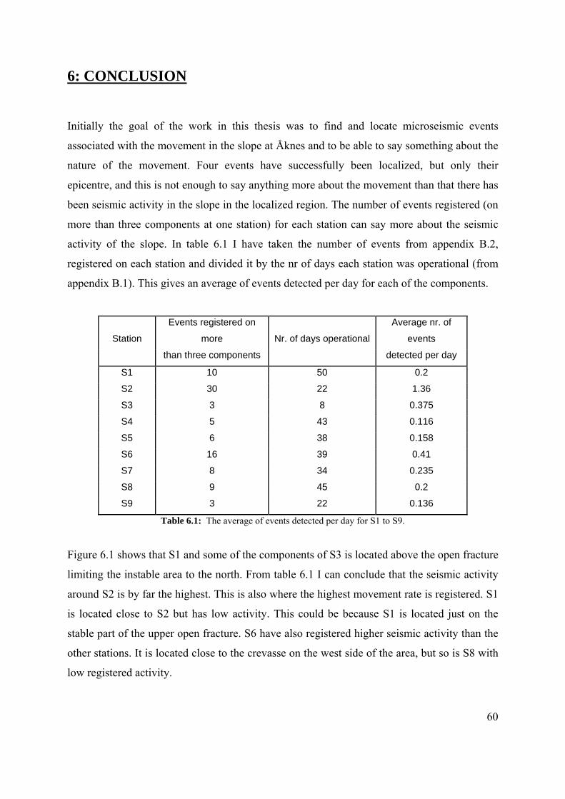
6: CONCLUSION

Initially the goal of the work in this thesis was to find and locate microseismic events

associated with the movement in the slope at Åknes and to be able to say something about the

nature of the movement. Four events have successfully been localized, but only their

epicentre, and this is not enough to say anything more about the movement than that there has

been seismic activity in the slope in the localized region. The number of events registered (on

more than three components at one station) for each station can say more about the seismic

activity of the slope. In table 6.1 I have taken the number of events from appendix B.2,

registered on each station and divided it by the nr of days each station was operational (from

appendix B.1). This gives an average of events detected per day for each of the components.

Station

Events registered on

more Nr. of days operational

Average nr. of

events

than three components detected per day

S1 10 50 0.2

S2 30 22 1.36

S3 3 8 0.375

S4 5 43 0.116

S5 6 38 0.158

S6 16 39 0.41

S7 8 34 0.235

S8 9 45 0.2

S9 3 22 0.136

Table 6.1: The average of events detected per day for S1 to S9.

Figure 6.1 shows that S1 and some of the components of S3 is located above the open fracture

limiting the instable area to the north. From table 6.1 I can conclude that the seismic activity

around S2 is by far the highest. This is also where the highest movement rate is registered. S1

is located close to S2 but has low activity. This could be because S1 is located just on the

stable part of the upper open fracture. S6 have also registered higher seismic activity than the

other stations. It is located close to the crevasse on the west side of the area, but so is S8 with

low registered activity.

60

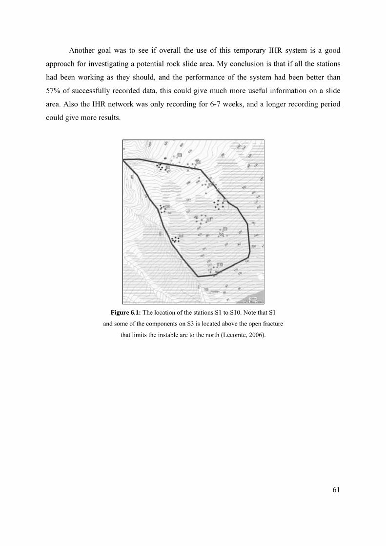
Another goal was to see if overall the use of this temporary IHR system is a good

approach for investigating a potential rock slide area. My conclusion is that if all the stations

had been working as they should, and the performance of the system had been better than

57% of successfully recorded data, this could give much more useful information on a slide

area. Also the IHR network was only recording for 6-7 weeks, and a longer recording period

could give more results.

Figure 6.1: The location of the stations S1 to S10. Note that S1

and some of the components on S3 is located above the open fracture

that limits the instable are to the north (Lecomte, 2006).

61

7: REFERENCES Ambuter B. P. and Solomon S. C. (1974). An Event-Recording System for Monitoring

Small Earthquakes. Bulletin of the Seismological Society of America. Vol. 64, No 4, pp.

1181-1188.

Blikra L. H. Anda E., Belsby S., Jogerud K., Klempe Ø. (2006). Åknes/Tafjord prosjektet,

Status rapport for Arbeidrgruppe 1 (Undersøking og overvåkning)

Blikra L. H. (2006). The Åknes/Tafjord project, status and plans for 2006. Published by

NGU (Norges Geologiske Undersøkelse) at Tafjord Project Workshop 20/2-21/2 2006,

Trondheim.

Bonnefoy-Claudet S., Cotton F. & Bard P. (2006). The nature of noise wavefield and its

applications for site effects studies, A literature review. Earth-Science Reviews 79 205-227.

Brenguier F., Coutant O., Dietrich M., Lecomte I. (2005). High resolution seismic imaging

of highly heterogeneous media: An experiment on the Puy des Goules volcano, France.

Geophysical Research Abstracts, vol 7, 06548, EGU Annual Meeting, Vienna.

Derron M. H., Blikra L. H., Jaboyedoff M. (2005). High resolution digital levation model

analysis for landslide hazard assessment (Åkerneset, Norway). Landslide and avalanches

ICFL 2005 Norway. Taylor & Francis Group, London.

Delarue C. (2006). Analysis of Microseismic Events Recorded at the Unstable Rock-Slope

Site at Åknes, Norway. Diplome d’ingenieur geophysicien, EOST, University of Strasburg I,

France.

Dietrich M., Lecomte I., Meric O., Roth M., Dore F., Guiguet R., De Barros L., Grasso J. –R.

& Orengo Y. (2006). Åknes 2005 campaign: refraction seismics and IHR microseismic

network. Åknes/Tafjord workshop 20-21.2.2006, Trondheim.

62

Eidsvig U. & Harbitz C. B. (2005) Innledende numeriske analyser av flodbølger som følge av

mulige skred fra Åkneset. Report from NGI published at the homepages of the Åknes/Tafjord

project. http://www.aknes-tafjord.no/Artikkel.aspx?AId=494&back=1&MId1=568&.

Emblemsvåg J. (2008), Flodbølger fra Åkneset, Kolofon Forlag AS.

Furseth A. (1985). Dommedagsfjellet: Tafjord 1934. Gyldendal Norsk Forlag. Norway.

Frery E. (2007). Seismic velocities of the unstable rock slope site at Åknes, Norway. Report

from a summer job at NORSAR, not published.

Ganerød G. V., Grøneng G., Rønning J. S., Dalsegg E., Elvebakk H., Tønnesen J. F.,

Kveldsvik V., Eiken T., Blikra L. H., Braathen A. (2008), Geological model of the Åknes

rockslide, western Norway, Engineering Geology 102 (2008) 1-18.

Høst J. (2006), Store Fjellskred i Norge, NGU Trondheim.

Lecomte I. (2006). Geophysics for investigation and analysis of large landslides. NFR

BILAT # 169822/D15, NORSAR/LGIT Final Report.

Musset A. E. & Khan M. A. (2000). Looking into the Earth. Cambridge University Press.

Cambridge, United Kingdom.

NGU (Norges Geologiske Undersøkelse) (2008). Berggrunnen i Norge N250. NGU,

Trondheim, Norway. Downloaded from http://www.ngu.no/kart/bg250/ December, 2008.

Roth M., Dietrich M., Blikra L. H., Lecomte I. (2005). Seismic Monitoring of the Unstable

Rock slope at Åknes, Norway. Extended abstract, 19th annual SAGEEP (Symposium on the

Application of Geophysics to Engineering and Environmental Problems), Seattle,

Washington.

63

Roth M. (2006). Status report 1-2006 Passive seismic monitoring at Åknes. Published at the

homepages of the Åknes-Tafjord project 2006 http://aknes-

tafjord.no/artikkel.aspx?MId1=578&AId=633&Back=1

Stein S. & Wysession M. (2003) An Introduction to seismology, earthquakes, and earth

structure. Blackwell Publishing. Oxford, UK.

Trnkoczy A. (1998). Understanding & Setting STA/LTA Trigger Algorithm Parameters for

the K2. Published at ftp://ftp.kinemetrics.com/pub/AppNotes/appnote41.PDF

Thorne M. (2004) rsac.m, http://web.utah.edu/thorne/saclab/rsac.m

Tveten E., Lutro O., Thorsnes T. (1998). Berggrunnskart Ålesund 1:250 000, (Ålesund,

western Norway). NGU Trondheim (bedrock map).

64

APPENDIX A: Matlab PROGRAMS Appendix A.1: rsac.m (Thorne M. 2004).

%RSAC Read SAC binary files. % RSAC('sacfile') reads in a SAC (seismic analysis code) binary % format file into a 3-column vector. % Column 1 contains time values. % Column 2 contains amplitude values. % Column 3 contains all SAC header information. % Default byte order is big-endian. M-file can be set to default % little-endian byte order. % % usage: output = rsac('sacfile') % % Examples: % % KATH = rsac('KATH.R'); % plot(KATH(:,1),KATH(:,2)) % % [SQRL, AAK] = rsac('SQRL.R','AAK.R'); % % by Michael Thorne (4/2004) mthorne@asu.edu function [varargout] = rsac(varargin); for nrecs = 1:nargin sacfile = varargin{nrecs}; %--------------------------------------------------------------------------- % Default byte-order % endian = 'big-endian' byte order (e.g., UNIX) % = 'little-endian' byte order (e.g., LINUX) endian = 'little-endian'; if strcmp(endian,'big-endian') fid = fopen(sacfile,'r','ieee-be'); elseif strcmp(endian,'little-endian') fid = fopen(sacfile,'r','ieee-le'); end % read in single precision real header variables: %--------------------------------------------------------------------------- for i=1:70 h(i) = fread(fid,1,'single'); end % read in single precision integer header variables:

65

%--------------------------------------------------------------------------- for i=71:105 h(i) = fread(fid,1,'int32'); end % Check header version = 6 and issue warning %--------------------------------------------------------------------------- % If the header version is not NVHDR == 6 then the sacfile is likely of the % opposite byte order. This will give h(77) some ridiculously large % number. NVHDR can also be 4 or 5. In this case it is an old SAC file % and rsac cannot read this file in. To correct, read the SAC file into % the newest verson of SAC and w over. % if (h(77) == 4 | h(77) == 5) message = strcat('NVHDR = 4 or 5. File: "',sacfile,'" may be from an old version of SAC.'); error(message) elseif h(77) ~= 6 message = strcat('Current rsac byte order: "',endian,'". File: "',sacfile,'" may be of opposite byte-order.'); error(message) end % read in logical header variables %--------------------------------------------------------------------------- for i=106:110 h(i) = fread(fid,1,'int32'); end % read in character header variables %--------------------------------------------------------------------------- for i=111:302 h(i) = (fread(fid,1,'char'))'; end % read in amplitudes %--------------------------------------------------------------------------- YARRAY = fread(fid,'single'); if h(106) == 1 XARRAY = (linspace(h(6),h(7),h(80)))'; else error('LEVEN must = 1; SAC file not evenly spaced') end % add header signature for testing files for SAC format %--------------------------------------------------------------------------- h(303) = 77; h(304) = 73; h(305) = 75;

66

h(306) = 69; % arrange output files %--------------------------------------------------------------------------- OUTPUT(:,1) = XARRAY; OUTPUT(:,2) = YARRAY; OUTPUT(1:306,3) = h(1:306)'; %pad xarray and yarray with NaN if smaller than header field if h(80) < 306 OUTPUT((h(80)+1):306,1) = NaN; OUTPUT((h(80)+1):306,2) = NaN; end fclose(fid); varargout{nrecs} = OUTPUT; end end Appendix A.2: findevents.m

function [A] = findevents(sacfil,argin)

a = str2num(argin(32)); %This is done to make the header information b = str2num(argin(34)); %into an integer to avoid printing problems c = str2num(argin(35)); %later. d = str2num(argin(37)); e = str2num(argin(38)); %f = str2num(argin(15)); %scipping the minutes and seconds to make the %g = str2num(argin(16)); %number have fewer digits. %h = str2num(argin(18)); %i = str2num(argin(19)); j = str2num(argin(47)); k = str2num(argin(53));

l = [a b c d e j k]; %make a matrix with the digits from the header. header1 = sprintf('%1d',l); %making one string from the elements of l. header = str2num(header1); %convertng the string into an integer.

nr = size(sacfil); %The size of the sacfile gives the nr of N = nr(1,1); %samplingpoints N.

67

K = [1:N]; %gives the first colomb the nr of

- %samplingpoint.

sacfil(:,1) = K;

%lta = std(sacfil(:,2)); %to keep the lta the same value.(doesn't work)

event = [0 0 0]; %event = zeros(10,3); %Define a matrix that holds the registered j = 0; %events if any. j counts.

stalta = zeros(1,N); %Define vektor that holds the values of %STA/LTA. %n1 = 120000; %Long term average in nr of samplingpoints. %n2 = 32000; %Short term average. %begin = 1.5; %Treshold for registrering an event. %finish = 1.5; %Treshold for stop registrering.

n1 = 500; n2 = 50; begin = 3; finish = 3;

regevent = 0; %to test if registration should be done.

for i = 1:10:N-n1 y = i+n1-n2; %if regevent == 0 %When an event is registered % lta = std(sacfil(i:x,2)); %the LTA will keep it's value %end %untill the stalta reach stop. %(this takes to long) lta = std(sacfil(i:i+n1,2)); sta = std(sacfil(y:i+n1,2)); stalta(i) = sta/lta;

if (stalta(i) >= begin) & (regevent == 0) j = j+1;

68

event(j,1) = i; regevent = 1; end

if (stalta(i) <= finish) & (regevent == 1) event(j,2) = i; event(j,3) = header; regevent = 0; end

%if mod(i,1000) == 0 %loop to follow the calculation on screen, % i %prints out avery 100 i. %end end

R = max(sacfil(:,2)); S = min(sacfil(:,2)); figure subplot(2,1,1); plot(stalta); title('STA/LTA') xlabel('samplingpoint 900000 pr hour'); ylabel('STA/LTA') title(argin) subplot(2,1,2); plot(sacfil(:,1),sacfil(:,2)); title('Seismogram') ylim([S R]) xlabel('sampling (250 pr sec)'); ylabel('amplitude')

%plot(sacfil(:,1),sacfil(:,2)); title('Seismogram') %ylim([S R]) %xlabel('sampling (250 pr sec)'); ylabel('amplitude')

A = event;

Appendix A.3: makefilenames.m

fid = fopen('/mn/sokrates/geo-master-u1/mariahn/mastern/281-

290filelist.allstations','r');

tline = fgetl(fid); [x] = strtok(tline);

69

filenames = x; eof = 0; while (eof == 0) tline = fgetl(fid); if(tline == -1) eof = -1; break; end [x] = strtok(tline); filenames = [filenames;x]; end

Appendix A.4: runfiles.m

a = size(filenames); n = a(1,1);

for i=1:n fid = fopen('found9','a'); M = rsac(filenames(i,:)); event = find2(M,filenames(i,:)); a = size(event); b = a(1,1);

if event(1,1)>0 fprintf(fid,'%s\n',filenames(i,:));

for j=1:b fprintf(fid,'%d,%d,%d\n',event(j,:)); end end

fclose(fid);

end

70

Appendix A.5: findvelSPall.m

function [A] = findvelSPall t1 = 113100003.94; %Trigger times plus a delay of 3.94 msec. t2 = 125200003.94; t3 = 134800003.94; t4 = 080900003.94; t5 = 091700003.94; load artime %first coloumb contains the nr of the stations, the load distSPall %following coulombs sontains the arival times and the %distances to the five shotpoints. j = 1; k = 1; l = 1; m = 1; n = 1; for i = 1:90 if artime(i,2) > 0 v1(j,2) = distSPall(i,2)/(artime(i,2)-t1); v1(j,1) = distSPall(i,1); v1(j,3) = distSPall(i,2); v1(j,4) = artime(i,2)-t1; j = j+1; end end for i = 1:90 if artime(i,3) > 0 v2(k,2) = distSPall(i,3)/(artime(i,3)-t2); v2(k,1) = distSPall(i,1); v2(k,3) = distSPall(i,3); v2(k,4) = artime(i,3)-t2; k = k+1; end end for i = 1:90 if artime(i,4) > 0 v3(l,2) = distSPall(i,4)/(artime(i,4)-t3); v3(l,1) = distSPall(i,1); v3(l,3) = distSPall(i,4); v3(l,4) = artime(i,4)-t3; l = l+1; end end for i = 1:90 if artime(i,5) > 0 v4(m,2) = distSPall(i,5)/(artime(i,5)-t4); v4(m,1) = distSPall(i,1); v4(m,3) = distSPall(i,5); v4(m,4) = artime(i,5)-t4; m = m+1;

71

end end for i = 1:90 if artime(i,6) > 0 v5(n,2) = distSPall(i,6)/(artime(i,6)-t5); v5(n,1) = distSPall(i,1); v5(n,3) = distSPall(i,6); v5(n,4) = artime(i,6)-t5; n = n+1; end end %The content of the velocity matrixes v1, v2, v3, v4 and v5: %coulomb 1: the komponents number. (with a number one in front) %coulomb 2: the calculated velocity. %coulomb 3: the direct distance from the shotpoint. %coulomb 4: the traveltimes. av1 = sum(v1(:,2))/j; av2 = sum(v2(:,2))/k; av3 = sum(v3(:,2))/l; av4 = sum(v4(:,2))/m; av5 = sum(v5(:,2))/n; B = [v1;v2;v3;v4;v5]; avAll = sum(B(:,2))/(j+k+l+m+n) %Want to plot the traveltimes vs increasing distance from the shot point to %find a velocity gradient with depth. The longer the waves have traveled, %the deeper the waves have traveled. scatter(B(:,3),B(:,4)) xlabel('distance from SP') ylabel('traveltime ms') figure scatter(v1(:,3),v1(:,4),'r') xlabel('distance from SP') ylabel('traveltime ms') hold on scatter(v2(:,3),v2(:,4),'b') scatter(v3(:,3),v3(:,4),'g') scatter(v4(:,3),v4(:,4),'y') scatter(v5(:,3),v5(:,4),'m') legend('v1','v2','v3','v4','v5') A = [av1;av2;av3;av4;av5];

Appendix A.6: lokalisering.m

% map the misfit to localize microevents in Aaknes format COMPACT format SHORT G % load the positions of the stations in East-North-altitude load positions; pos=positions;

72

clear positions; [nstat,ncoord]=size(pos); % calculate positions relative to component S1-3 (northernmost station, % almost at the top) iref=3; for i=1:nstat; posrel(i,:)=pos(i,:)-pos(iref,:); end; posrel; meanelv=mean(posrel(:,3)) stdelv=std(posrel(:,3)) % rotate the coordinate system to get horizontal coordinates in max-dip - % along topo system and turn to get positive downwards h=4.; % reference moved 4 meters below point 3 to get best % fit of ref. plane alpha=72.; % azimuth of along-topo lines, in degrees dip=35.9; % dip of plane rot1=[cosd(alpha), -sind(alpha),0.; sind(alpha),cosd(alpha),0.; 0.,0.,1.]; rot2=[cosd(dip), 0., -sind(dip); 0.,1.,0.; sind(dip),0.,cosd(dip)]; for i=1:nstat; temp=posrel(i,:)'; temp(3)=temp(3)+h; temp=rot1*temp; temp=rot2*temp; temp(3)=-temp(3); posrot(i,:)=temp'; end; % check the values of the average and standard deviations of new vertical % coordinate to verify the plane has been chosen properly posrot; meanelv=mean(posrot(:,3)) stdelv=std(posrot(:,3)) %------------------------------------------------------------------------- %locations of the five shots locSP = [395362,6895946,772;395512,6895725,572;395598,6895552,440;395629,6895355,324;395679,6895103,142]; for i=1:5 locrel(i,:)=locSP(i,:)-pos(iref,:); end for i=1:5 temploc = locrel(i,:)'; temploc=rot1*temploc; temploc=rot2*temploc; locSProt(i,:)=temploc; end %-------------------------------------------------------------------------- % load the arrival times of the microevents load eventArTimes; [nstat2,nevent]=size(eventArTimes); if (nstat2~=nstat)

73

disp ('discrepancy in number of stations in the two files') end % dimensions of the search timeinterval=120; % time interval before minimum read time, % for which the search will be done in ms xmin=-400; % up and downdip coordinate xmax=1400; ymin=-500; % strike coordinate ymax=500; % increments in the search dt=120; dx=20.; dy=20; %initialize arrays related to the search xnodes=xmin:dx:xmax; ynodes=ymin:dy:ymax; tnodes=-120:dt:timeinterval; %note this has to be used backwards in time nx=length(xnodes); ny=length(ynodes); nt=length(tnodes); %------------------------------------------------------------------------- %tnode for event nr 2 is 88 %tnode for event nr 3 is 38 %tnode for event nr 4 is 10 3%tnode for event nr 5 is 29 %tnode for event nr 6 is %tnode for event nr 7 is %tnode for event nr 8 is %-------------------------------------------------------------------------- % initialize the parameters of the theoretical traveltime curve t0 = 44; % 44 ms slowness=0.19; % 0,19 ms/m %for i=2:nevent; % start on 2 because first column is not an event for i=7:7; for j=1:nstat2; if (eventArTimes(j,i)~=0); tt(j)=eventArTimes(j,i); % fill inn a vector else tt(j)=NaN; end; %put all the zeroes as NaN end tmin= min(tt); % tmin used as reference time from then on for ix=1:nx; for iy=1:ny; for it=1:nt; misfit(ix,iy,it)=0; for is=1:nstat2; if (~isnan(tt(is))); dist= sqrt( (xnodes(ix)-posrot(is,1))^2 + (ynodes(iy)-posrot(is,2))^2 ); traveltheo = t0 + slowness*dist; % theoretical traveltime travelmeas = tt(is)-tmin+tnodes(it);

74

% measured traveltime if source was tnodes(it) before tmin dmisfit = (travelmeas-traveltheo)^2; misfit(ix,iy,it)= misfit(ix,iy,it)+dmisfit ; end; end; end end end m1=min(misfit,[],1); m2=min(m1,[],2) m1=max(misfit); m2=max(m1); m3=max(m2); lines=50; colorvec=linspace(0,m3,50); for it=1:nt; figure slice=misfit(:,:,it); contour(xnodes,ynodes,slice',colorvec) colorbar A = contour(xnodes,ynodes,slice',colorvec); clabel(A) xlabel('Down slope in m') ylabel('Along strike in m') hold on scatter(posrot(:,1),posrot(:,2),'m') scatter(locSProt(:,1),locSProt(:,2),'r','*') end end;

75

APPENDIX B: TABLES

Appendix B.1: Table of files run in findevents.m. The day and station marked with an x is

successfully run. The days and stations marked with – does not exist in the data.

dag/stasjon 1 2 3 4 5 6 7 8 9 10 filelist name:

event is

stored in:

240-28/8 x x x x x x x x - - 240-

243filelist.allstations found2

241-29/8 x x x x x x x x - - 240-

243filelist.allstations found2

242-30/8 x x x x x x x x x - 240-

243filelist.allstations found2

243-31/8 x x x x x x x x x - 240-

243filelist.allstations found2

x x [0-6] x x x x x x L

244-247filelist-allstations found31/9 244

2/9 245 x x - x x x x x x L 244-247filelist-

allstations found3

3/9 246 x x - x x x x x x L 244-247filelist-

allstations found3

4/9 247 x x - x x x x x x L 244-247filelist-

allstations found3

5/9 248 x x - x x x x x x L 248-

251filelist.allstations found4

x [0-6] - x x x x x x L

248-251filelist.allstations found46/9 249

7/9 250 x - - x x x x x x [0-6]

248-251filelist.allstations found4

8/9 251 x - - x x x x x x - 248-

251filelist.allstations found4

9/9 252 x - - x x x x x x - 252-

255filelist.allstations found5

10/9 253 x - - x x x x x x - 252-

255filelist.allstations found5

11/9 254 x - - x - x x x x - 252-

255filelist.allstations found5

12/9 255 x x - x - x x x [0-6] -

252-255filelist.allstations found5

13/9 256 x x - x - x x x - - 256-

260filelist.allstations found6

14/9 257 x x - x - x x x - - 256-

260filelist.allstations found6

15/9 258 x x - x - x x x - - 256-

260filelist.allstations found6

16/9 259 x x - x - x x x - - 256-

260filelist.allstations found6

17/9 260 x x - x - x x [0-6] - -

256-260filelist.allstations found6

18/9 261 x - - x - x x - - - 261-

270filelist.allstations found7

76

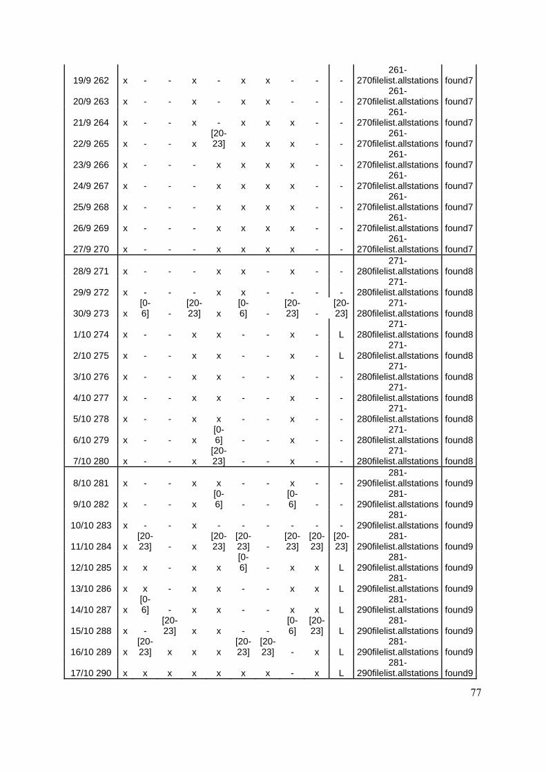
19/9 262 x - - x - x x - - - 261-

270filelist.allstations found7

20/9 263 x - - x - x x - - - 261-

270filelist.allstations found7

21/9 264 x - - x - x x x - - 261-

270filelist.allstations found7

x - - x [20-23] x x x - -

261-270filelist.allstations found722/9 265

23/9 266 x - - - x x x x - - 261-

270filelist.allstations found7

24/9 267 x - - - x x x x - - 261-

270filelist.allstations found7

25/9 268 x - - - x x x x - - 261-

270filelist.allstations found7

26/9 269 x - - - x x x x - - 261-

270filelist.allstations found7

27/9 270 x - - - x x x x - - 261-

270filelist.allstations found7

28/9 271 x - - - x x - x - - 271-

280filelist.allstations found8

29/9 272 x - - - x x - - - - 271-

280filelist.allstations found8

x [0-6] -

[20-23] x

[0-6] -

[20-23] -

[20-23]

271-280filelist.allstations found830/9 273

1/10 274 x - - x x - - x - L 271-

280filelist.allstations found8

2/10 275 x - - x x - - x - L 271-

280filelist.allstations found8

3/10 276 x - - x x - - x - - 271-

280filelist.allstations found8

4/10 277 x - - x x - - x - - 271-

280filelist.allstations found8

5/10 278 x - - x x - - x - - 271-

280filelist.allstations found8

x - - x [0-6] - - x - -

271-280filelist.allstations found86/10 279

x - - x [20-23] - - x - -

271-280filelist.allstations found87/10 280

8/10 281 x - - x x - - x - - 281-

290filelist.allstations found9

x - - x [0-6] - -

[0-6] - -

281-290filelist.allstations found99/10 282

10/10 283 x - - x - - - - - - 281-

290filelist.allstations found9

x [20-23] - x

[20-23]

[20-23] -

[20-23]

[20-23]

[20-23]

281-290filelist.allstations found911/10 284

12/10 285 x x - x x [0-6] - x x L

281-290filelist.allstations found9

13/10 286 x x - x x - - x x L 281-

290filelist.allstations found9

x [0-6] - x x - - x x L

281-290filelist.allstations found914/10 287

x - [20-23] x x - -

[0-6]

[20-23] L

281-290filelist.allstations found915/10 288

x [20-23] x x x

[20-23]

[20-23] - x L

281-290filelist.allstations found916/10 289

17/10 290 x x x x x x x - x L 281-

290filelist.allstations found9

77

Appendix B.2: This table shows all the events that has been registered on more than four

components. The events that have been registered on more than two stations are marked with

gray and given a number in the last column.

Station Day hour

start

time end time komponents

from found

file Eventnr:

S2 240 22 773161 773241 0,1,2,4,5,7 found2 1

S3 240 22 773271 773341 0,2,3,4,5 found2 1

S4 240 22 773321 773411 0,1,3,4,5,6,7,8 found2 1

S5 240 22 773141 773191 0,1,2,3,5 found2 1

S6 240 22 773301 773351 1,2,3,4,5,6,7,8 found2 1

S6 240 23 321741 321811 1,2,3,4,5,6,7,8 found2

S7 240 22 773231 773301 3,4,6,7,8 found2

S2 241 2 79031 79091 1,4,5,6,7 found2

S6 241 21 187791 187831 0,2,3,6,8 found2

S5 242 21 112391 112451 0,1,2,5 found2 2

S6 242 21 112371 112441 1,2,3,4,5,6,7,8 found2 2

S7 242 21 112461 112531 0,2,3,4,5,6,7,8 found2 2

S8 242 21 112301 112371 1,2,3,4,5,6,7,8 found2 2

S9 242 21 112401 112471 1,2,3,4,5,6 found2 2

S2 243 0 516711 516821 1,2,4,5,6,7 found2

S7 243 6 421401 421461 0,2,3,4,7,8 found2

S7 243 6 722391 722491 0,3,4,5,6,7,8 found2

S3 244 3 292761 292821 0,1,2,3,4,5 found3

S2 245 0 395941 395991 1,2,4,5,6,7,8 found3

S6 245 6 346461 346601 1,2,3,4,6,7,8 found3

S7 245 20 238261 238201 1,2,3,4,7 found3

S5 247 21 253321 253401 0,1,2,3,5,6 found3 3

S6 247 21 253281 253341 1,2,3,4,5,6,8 found3 3

S7 247 21 253491 253571 0,2,3,4,5,6,7,8 found3 3

S8 247 21 253391 253461 0,1,3,4,5,6,7,8 found3 3

S9 247 21 252401 253471 1,2,4,6 found3 3

S1 248 2 378931 378981 2,5,7,8 found4 4

S1 248 5 570161 570211 0,1,2,3,5,6 found4 5

S2 248 1 709681 709791 all !! found4

S2 248 2 378851 378951 all !! found4 4

S2 248 4 513751 513831 1,3,4,6,7,8 found4

S2 248 5 570121 570221 all !! found4 5

78

S2 248 20 566161 566231 4,5,6,7,8 found4

S4 248 5 570061 570121 1,4,5,6,8 found4 5

S8 248 22 496911 496971 0,1,4,8 found4

S2 249 4 628161 628231 0,1,2,5,6,7,8 found4

S2 249 6 720661 720721 1,4,6,7 found4

S6 252 2 810471 810531 1,3,5,6,7,8 found5

S1 253 4 247171 247221 1,6,7,8 found5

S1 253 6 540581 540631 0,1,3,5,6,7,8 found5 6

S6 253 3 415771 415851 3,5,6,7,8 found5

S6 253 6 540601 540681 1,2,3,4,5,6,7,8 found5 6

S6 253 20 790951 790961 1,3,4,5,6,7,8 found5

S8 253 5 222501 222551 2,4,5,8 found5

S8 254 21 732941 732991 0,1,4,5,7,8 found5

S1 255 4 17551 17601 0,1,3,6,7,8 found5

S1 255 4 561671 561721 0,6,7,8 found5

S2 255 6 34101 34141 0,1,2,3,4 found5

S2 255 20 51141 51221 0,1,2,4,5,6,7,8 found5

S2 255 22 811541 811601 1,5,6,8 found5

S6 256 1 501181 501251 3,5,6,7,8 found6

S2 257 20 669251 669311 3,6,7,8 found6

S2 257 21 518501 518551 0,2,6,7 found6

S2 257 22 680001 680071 0,1,2,7,8 found6

S1 258 5 749851 749921 0,2,3,5,6 found6

S2 258 6 659221 659351 all !! found6

S6 258 6 42501 42551 1,2,3,5,6,7,8 found6

S6 258 6 308361 208681 5,6,7,8 found6

S2 259 0 593961 594081 0,1,2,6,7,8 found6

S2 259 1 766861 766921 0,2,6,7,8 found6

S2 259 20 82291 82311 0,3,4,6,7 found6

S2 259 22 626811 626861 2,3,6,7,8 found6

S2 259 23 386861 386911 1,2,3,4,5,6,7,8 found6

S2 260 1 773221 773291 all !! found6

S2 260 4 2181 2221 1,2,3,4,5,6,7,8 found6

S2 260 5 245721 245751 4,5,6,7,8 found6

S6 260 2 381001 381071 1,3,5,6,7,8 found6

S6 260 5 110181 110221 1,3,5,6,7,8 found6

S6 261 20 345251 345261 3,4,5,6,7,8 found7

S7 262 4 852871 852901 2,6,7,8 found7

S1 267 20 212271 212321 0,1,6,7,8 found7

79

S6 267 4 806561 806611 3,5,6,8 found7

S8 267 0 571531 571581 0,6,7,8 found7

S8 270 1 43921 43991 1,4,6,7,8 found7

S8 270 6 453191 453201 1,4,5,6,7 found7

S6 271 3 67971 67981 1,6,7,8 found8

S1 272 1 357501 357551 0,1,6,7,8 found8

S8 285 20 601001 601031 2,6,7,8 found9

S1 287 3 64191 64241 0,1,3,5,6,7,8 found9

S2 287 3 64191 64241 all !! found9

S4 288 6 678061 678141 2,3,4,5,6,7,8 found9 7

S4 288 6 684861 684901 2,3,4,5,6,7,8 found9 8

S5 288 6 677811 677851 0,4,6,7,8 found9 7

S5 288 6 684621 684671 0,4,6,7,8 found9 8

S5 288 6 893731 893771 0,1,3,4,5,6,7,8 found9

S2 289 20 668191 668291 2,5,6,7 found9

S3 289 4 590091 590141 2,3,4,5 found9

S5 289 1 367191 367231 3,6,7,8 found9

S2 290 4 411481 411521 0,1,6,7,8 found9

S2 290 20 145771 145801 2,3,4,5,6,7,8 found9

S4 290 6 603141 603171 1,2,3,5,7 found9

S7 290 2 595461 595471 1,2,6,7 found9

S9 290 5 554031 554081 4,5,6,7,8 found9

Appendix B.3: Positions and times for the five shots from the refraction seismic survey

(Frery 2007).

80

Appendix B.4: Position of all the components. The 3-component geophones are marked with

bold letters. Here the components are not labeled the same way as in the data, the two first

columns of appendix B.5 shows the correspondence.

81

82

Appendix B.5: The picked arrival times for the five active shots SP1 to SP2. The first column

is the komponent number for all the station as they are numbered in the data. In the second

column is the corresponding number of the components as they are labeled when the

coordinates were measured in the field. In the second column the 3-component geophone is

marked with bold numbers. Such that for example for Station 5m the components 1,2 and

three in the data are those which is in the 3-comopnent geophone.

Data Frery SP1 SP2 SP3 SP4 SP5

S1 S1

0 1 11.31.00.096 12.52.00.122 13.48.00.165

1 2 11.31.00.103 12.52.00.128 13.48.00.173

2 3 11.31.00.137 12.52.00.123

3 4_1

4 4_2

5 4_3

6 5 11.31.00.094

7 6 11.31.00.132 12.52.00.131

8 7

S2 S2

0 1 11.31.00.107 12.52.00.170 09.17.00.312

1 2 11.31.00.078 12.52.00.153 09.17.00.282

2 3 11.31.00.102 12.52.00.157 13.48.00.204

3 4 11.31.00.064

4 5 11.31.00.053 12.52.00.147

5 6 13.48.00.201

6 7_1

7 7_2

8 7_3

S3 S3

0 1 11.31.00.090 12.52.00.103 13.48.00.145

1 2 11.31.00.096 12.52.00.112 08.09.00.184

2 3 11.31.00.092 12.52.00.115 13.48.00.155 08.09.00.187

3 4_1

4 4_2

5 4_3

6 5

7 6

83

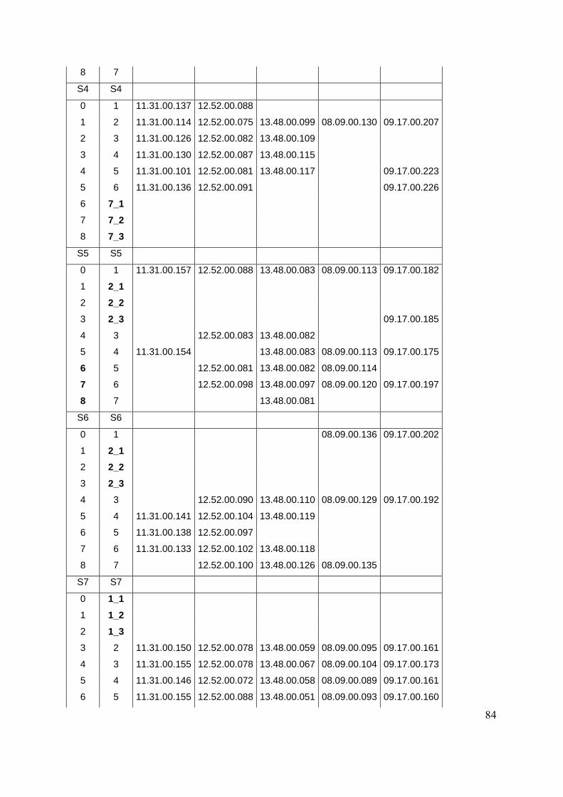
8 7

S4 S4

0 1 11.31.00.137 12.52.00.088

1 2 11.31.00.114 12.52.00.075 13.48.00.099 08.09.00.130 09.17.00.207

2 3 11.31.00.126 12.52.00.082 13.48.00.109

3 4 11.31.00.130 12.52.00.087 13.48.00.115

4 5 11.31.00.101 12.52.00.081 13.48.00.117 09.17.00.223

5 6 11.31.00.136 12.52.00.091 09.17.00.226

6 7_1

7 7_2

8 7_3

S5 S5

0 1 11.31.00.157 12.52.00.088 13.48.00.083 08.09.00.113 09.17.00.182

1 2_1

2 2_2

3 2_3 09.17.00.185

4 3 12.52.00.083 13.48.00.082

5 4 11.31.00.154 13.48.00.083 08.09.00.113 09.17.00.175

5 12.52.00.081 13.48.00.082 08.09.00.114 6 6 12.52.00.098 13.48.00.097 08.09.00.120 09.17.00.197 7 7 13.48.00.081 8

S6 S6

0 1 08.09.00.136 09.17.00.202

1 2_1

2 2_2

3 2_3

4 3 12.52.00.090 13.48.00.110 08.09.00.129 09.17.00.192

5 4 11.31.00.141 12.52.00.104 13.48.00.119

6 5 11.31.00.138 12.52.00.097

7 6 11.31.00.133 12.52.00.102 13.48.00.118

8 7 12.52.00.100 13.48.00.126 08.09.00.135

S7 S7

0 1_1

1 1_2

2 1_3

3 2 11.31.00.150 12.52.00.078 13.48.00.059 08.09.00.095 09.17.00.161

4 3 11.31.00.155 12.52.00.078 13.48.00.067 08.09.00.104 09.17.00.173

5 4 11.31.00.146 12.52.00.072 13.48.00.058 08.09.00.089 09.17.00.161

6 5 11.31.00.155 12.52.00.088 13.48.00.051 08.09.00.093 09.17.00.160

84

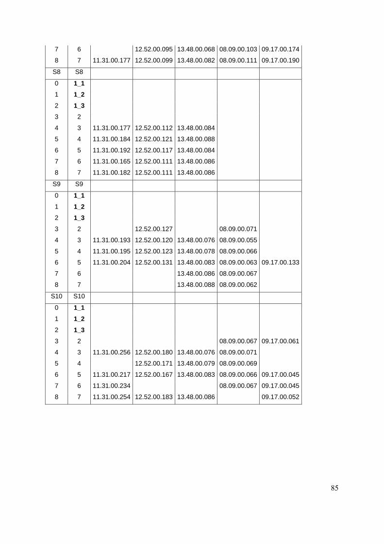
7 6 12.52.00.095 13.48.00.068 08.09.00.103 09.17.00.174

8 7 11.31.00.177 12.52.00.099 13.48.00.082 08.09.00.111 09.17.00.190

S8 S8

0 1_1

1 1_2

2 1_3

3 2

4 3 11.31.00.177 12.52.00.112 13.48.00.084

5 4 11.31.00.184 12.52.00.121 13.48.00.088

6 5 11.31.00.192 12.52.00.117 13.48.00.084

7 6 11.31.00.165 12.52.00.111 13.48.00.086

8 7 11.31.00.182 12.52.00.111 13.48.00.086

S9 S9

0 1_1

1 1_2

2 1_3

3 2 12.52.00.127 08.09.00.071

4 3 11.31.00.193 12.52.00.120 13.48.00.076 08.09.00.055

5 4 11.31.00.195 12.52.00.123 13.48.00.078 08.09.00.066

6 5 11.31.00.204 12.52.00.131 13.48.00.083 08.09.00.063 09.17.00.133

7 6 13.48.00.086 08.09.00.067

8 7 13.48.00.088 08.09.00.062

S10 S10

0 1_1

1 1_2

2 1_3

3 2 08.09.00.067 09.17.00.061

4 3 11.31.00.256 12.52.00.180 13.48.00.076 08.09.00.071

5 4 12.52.00.171 13.48.00.079 08.09.00.069

6 5 11.31.00.217 12.52.00.167 13.48.00.083 08.09.00.066 09.17.00.045

7 6 11.31.00.234 08.09.00.067 09.17.00.045

8 7 11.31.00.254 12.52.00.183 13.48.00.086 09.17.00.052

85

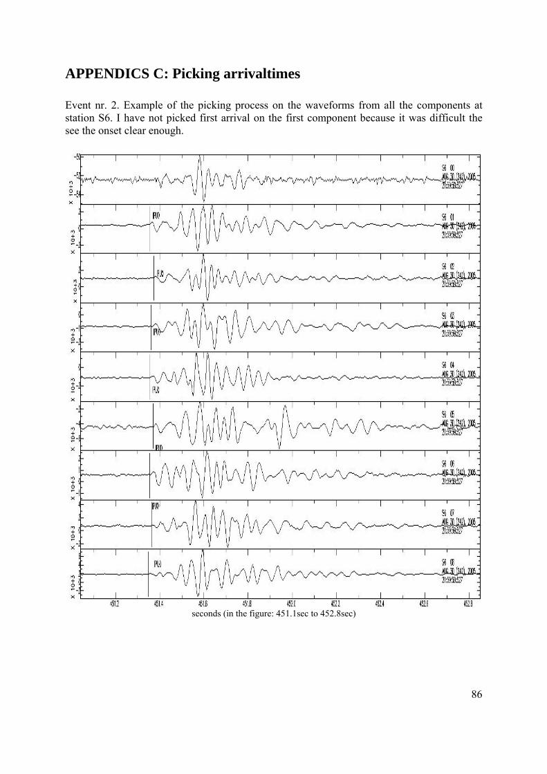
86

APPENDICS C: Picking arrivaltimes Event nr. 2. Example of the picking process on the waveforms from all the components at station S6. I have not picked first arrival on the first component because it was difficult the see the onset clear enough.

seconds (in the figure: 451.1sec to 452.8sec)