arX

iv:1

508.

0049

1v1

[he

p-th

] 3

Aug

201

5

Structural Theory of 2-d Adinkras

Kevin Iga and Yan X Zhang

August 4, 2015

Abstract

Adinkras are combinatorial objects developed to study (1-dimensional) su-persymmetry representations. Recently, 2-d Adinkras have been developed tostudy 2-dimensional supersymmetry. In this paper, we classify all 2-d Adinkras,confirming a conjecture of T. Hübsch. Along the way, we obtain other struc-tural results, including a simple characterization of Hübsch’s even-split doubly

even codes.

1 Introduction

Adinkras (in this paper, called 1-d Adinkras) were introduced in [8] to study repre-sentations of the super-Poincaré algebra in one dimension. There have been a numberof developments that have led to the classification of 1-d Adinkras.[2, 3, 4, 5, 6, 16]Based on the success of this program, there have been a few recent approaches tousing Adinkra-like ideas to study the super-Poincaré algebra in two dimensions. Thishas led to the development of 2-d Adinkras.[12, 13]

In this paper, we characterize 2-d Adinkras, guided by the approach and con-jectures set forth in [13]. We begin in Section 2 by recalling the definition of (1-d)Adinkras and some of their features, reviewing the code associated with an Adinkra[4]and the concept of vertex switching.[6, 16] As this paper is a mostly self-containedwork of combinatorial classification, we do not discuss (or require from the reader)the physics and representation theory background relating to 1-d Adinkras; the in-terested reader may see Appendix A and the aforementioned references for moreinformation along these lines. Instead, Section 2’s goal is to provide the minimumbackground to understand and manipulate Adinkras as purely combinatorial objects.

Then, Sections 3–5 discuss 2-d Adinkras: the definition, some basic constructions,and characterizing their codes. In Section 6, we prove the main theorem, which isHübsch’s conjecture:1

1The formulation in [13] is slightly different: see Appendix A for details.

1

Theorem 1.1. Let A be a connected 2-d Adinkra. Then there exist 1-d Adinkras A1

and A2 so that

A ∼= F (A1 × A2)/ ∼,

where F is a vertex switching and ∼ is described by an action of a subgroup of Zn2 .

Finally, Section 7, guided by the main theorem, summarizes the basic structure of2-d Adinkras, including a (computable but impractical due to combinatorial explo-sion) scheme to generate all 2-d Adinkras. We end with some remarks in Section 8.

2 Preliminaries

2.1 1-d Adinkras

Adinkras in [8, 2, 16] will be referred to as 1-d Adinkras in this paper, since theyrelate to supersymmetry in 1 dimension. In this section, we review a definition of1-d Adinkras and give some tools from previous work on their structural theory. Thematerial in this section is mainly found in [4, 16], with minor paraphrasing.

Definition 2.1 (1-d Adinkras). Let n be a non-negative integer. An 1-d Adinkrawith n colors is (V,E, c, µ, h) where:

1. (V,E) is a finite undirected graph (called the underlying graph of the Adinkra)with vertex set2 V and edge set E.

2. c : E → [n] := {1, . . . , n} is a map called the coloring. We require that forevery v ∈ V and i ∈ [n], there exists exactly one w ∈ V so that (v, w) ∈ Eand c(v, w) = i. We also require that every two-colored simple cycle be oflength 4 (A simple cycle is one which does not repeat vertices other than thestarting vertex; A two-colored cycle is one where the set of colors of the edgeshas cardinality 2).

3. µ : E → Z2 = {0, 1} is a map called the dashing. The parity of µ on a cyclegiven by vertices (v0, . . . , vk) is defined as the sum

k−1∑

i=0

µ(vi, vi+1) (mod 2).

We require that the parity of µ on every two-colored simple cycle to be odd.Such a dashing µ is called admissible.

2In [8, 2], there is also a bipartition of the vertices, where some vertices are represented by opencircles and called bosons, and other vertices are represented by filled circles and called fermions.This is not necessary to include in our definition, because the bipartition can be obtained directlyby taking the grading h modulo 2, which is a bipartition by property 4 below.

2

1

2

3

h

Figure 1: Example of a 1-d Adinkra with 3 colors. The coloring is represented bycolors on the edges. The dashing is represented by having a dashed edge if µ(e) = 1and a solid edge if µ(e) = 0. The grading is represented by the vertical height asindicated on the axis on the left.

4. h : V → Z is a map called the grading. We require that if (v, w) ∈ E, then|h(v)−h(w)| = 1. Equivalently, h provides a height function that makes (V,E)into the Hasse diagram of a ranked poset.

Figure 1 gives an example of a 1-d Adinkra.

2.2 Structural Aspects of 1-d Adinkras

Let A be a 1-d Adinkra with n colors, with vertex set V . For all i ∈ [n], defineqi : V → V such that for all v ∈ V , qi(v) is the unique vertex joined to v by an edgeof color i. In [4], it was shown that the map qi is a graph isomorphism (in fact, aninvolution) from the underlying graph of A to itself which preserves colors. The qicommute with each other. These facts can be used to combine the q1, . . . , qn mapsinto an action of Zn

2 on the graph (V,E) underlying the Adinkra in the followingway:

Definition 2.2. The action of Zn2 on the graph (V,E) underlying the Adinkra is

given on vertices by(x1, . . . , xn)v = qx1

1 ◦ · · · ◦ qxn

n (v).

Intuitively, the action of a sequence of bits, for instance, 11001, on a vertex isobtained by following edges with colors that correspond to 1’s in the sequence (inthis case, colors 1, 2, and 5). The fact that the qi’s commute implies that the orderof the colors does not matter.

The Adinkra A is connected if and only if the Zn2 action is transitive on the vertex

set of A. In this case the stabilizers of all vertices are equal (in general the stabilizersof two points in the same orbit are conjugate; here we know more since the groupis abelian). Define C(A), the code of the Adinkra A, to be this stabilizer. This is a

3

binary linear code of length n (i.e., a linear subspace of Zn2 ). As these are the only

types of codes we use, from now on we simply say code to mean “binary linear code.”

We call the elements of a code codewords. The weight of a codeword w is thenumber of 1’s in the word. A code is called even if all its codewords have evenweight. A code is called doubly-even if all its codewords have weight divisible by 4.An example of a doubly-even code is the span 〈111100, 001111〉, which has 22 = 4elements. An example of a code that is even but not doubly-even is the 1-dimensionalcode 〈11〉.

Codes are surprisingly relevant to the structural theory of Adinkras; in fact, oneshould basically think of the underlying graph of an Adinkra as a doubly-even code,as we now see.

2.3 Quotients

We now know that the stabilizer of our action on the graph is a code. We canalso go in the opposite direction: let In, the Hamming cube, be the graph with2n vertices labeled by strings of length n using the alphabet {0, 1}, with an edgebetween two vertices v and w if and only if they differ in exactly one place. Thereis a natural coloring on In: just color each edge by the coordinate where the twovertices differ. Now, codes in Zn

2 act on In by bitwise addition modulo 2, and theseare isomorphisms that preserve colors. A natural operation to consider on a coloredgraph Γ = (V,E, c) and a group C acting on V via graph isomorphisms that preservecolors is the quotient Γ/C, where the vertices are defined to be orbits in V/C, andwe have an c-colored edge (v, w) if and only if there is at least one c-colored edge(v′, w′) ∈ E with v′ in the orbit v and w′ in the orbit w.

Figure 2: Left: the colored graph I4. Middle: the quotient I4/{0000, 1111}. Right:as the code {0000, 1111} is doubly-even, there exists an Adinkra with the quotientas its underlying graph by Theorem 2.3.

Theorem 2.3. In/C is the colored graph of some 1-d Adinkra if and only if C is adoubly-even code.

See [4] for the original proof of this result. See [16] for a more general treatment

4

of quotienting by a code and a slightly extended correspondence3 between graphproperties of the quotient In/C and properties of the code C.

Figure 2 provides an example of a quotient of I4 by a code that obeys thistheorem. Encoded within the proof of Theorem 2.3 is the fact that if C is a doubly-even code, then there exists an admissible dashing. A constructive proof of existencecan be found in [5]. See [16] for an enumeration of all admissible dashings for anydoubly-even code.

2.4 Vertex Switching

Vertex switching was first introduced in the context of Adinkras in [8] and is morethoroughly set in its context in [6, 16].

Definition 2.4 (Vertex switching). Given an Adinkra A, and a vertex v of A, wedefine vertex switching at v to be the operation on A that returns a new Adinkra Awith the same vertices, edges, coloring, and grading but a new dashing µ so that

µ(e) =

{

1− µ(e), if e is incident to v

µ(e), otherwise.(2.5)

We leave to the reader to check that µ is still an admissible dashing; since the vertices,edges, coloring, and grading(s) are the same, A remains an Adinkra. We also use avertex switching of A to refer to a composition of vertex switchings at various verticesof A.

v

A

v

A

Figure 3: A vertex switching at v turns the Adinkra A on the left into the AdinkraA on the right. The two Adinkras have the same dashing except precisely the edgesthat are incident to v. Note that in both cases, each face of the cube has an oddnumber of dashed edges.

3Note that the quotient Γ/C does not necessarily retain nice properties of Γ; it does not evenhave to be a simple graph. It may also have edges with different colors between two vertices. Partof the work here is to show these pathologies do not happen when C is a doubly-even code.

5

In [7], vertex switching was first applied to dashings in Adinkras from a pointof view inspired by Seidel’s two-graphs [15].4 An enumeration of vertex switchingclasses leading to counting the number of dashings of any 1-d Adinkra can be foundin [16].

3 2-d Adinkras

Just as 1-d Adinkras were used to study 1-d supersymmetry, Gates and Hübschdeveloped 2-d Adinkras to study 2-d supersymmetry.[12, 13] We use a definitionhere that is equivalent to the one found there.5

A 2-d Adinkra is similar to a 1-d Adinkra except that some colors are called “left-moving” and the other colors called “right-moving”. Edges are called “left-moving”if they are colored by left-moving colors, and right-moving otherwise. Furthermore,there are two gradings, one that is affected by the left-moving edges and the otherfor the right-moving edges. More formally:

Definition 3.1 (2-d Adinkras). Let p and q be non-negative integers. A 2-d Adinkrawith (p, q) colors is a 1-d Adinkra (V,E, c, µ, h) with p + q colors, and two gradingfunctions hL : V → Z and hR : V → Z so that

• h(v) = hL(v) + hR(v).

• Let e be an edge. If c(e) ≤ p then e is called a left-moving edge; if c(e) > pthen it is called a right-moving edge. Similarly, the first p colors are calledleft-moving colors and the last q colors are called right-moving colors.

• if (v, w) is a left-moving edge, then |hL(v) − hL(w)| = 1 and hR(v) = hR(w).If (v, w) is a right-moving edge, then |hR(v)− hR(w)| = 1 and hL(v) = hL(w).

See Figure 4 for an example of a 2-d Adinkra. The main goal of this paper is tofollow the program set out in [13] and completely characterize 2-d Adinkras. As afirst step, we define the natural notion of products in the following section.

4 Products

One important way to produce a 2-d Adinkra with (p, q) colors is to take the productof two 1-d Adinkras (one with p colors, and the other with q colors), using thefollowing construction.

4In Seidel’s setting, vertex switching switched the existence of edges, not the sign of edges;this can be seen as equivalent our definition applied to the complete graph. The type of vertexswitching we do in this paper is sometimes called vertex switching on signed graphs in literaturefor disambiguation.

5The main notational difference is a kind of change of coordinates: there, nodes are labeled bymass dimension, which is hL+hR, and spin, which is hR−hL. Mass dimension is the units of massassociated with the field, where c = ~ = 1 and spin is the eigenvalue of x∂t + t∂x.

6

(0,0)

(1,0) (0,1)

(1,1)

Figure 4: A 2-d Adinkra with (2, 2) colors. The grading coordinates are given nextto the nodes as (hL, hR).

Construction 4.1. Let p and q be non-negative integers. Let A1 = (V1, E1, c1, µ1, h1)be a 1-d Adinkra with p colors and let A2 = (V2, E2, c2, µ2, h2) be a 1-d Adinkra qcolors. We define the product of these Adinkras A1 × A2 as the following 2-Adinkrawith (p, q) colors:

A1 × A2 = (V,E, c, µ, h1, h2)

where V = V1 × V2 and there are two kinds of edges in E:

• For every edge e in E1 connecting vertices v and w ∈ V1, and for every vertexx ∈ V2, we have an edge in E between vertices (v, x) and (w, x) in V = V1×V2

of color c1(e) and dashing µ1(e).

• For every edge e in E2 connecting vertices v and w ∈ V2 and for every vertexx ∈ V1, we have an edge in E between vertices (x, v) and (x, w) in V = V1×V2

of color p+ c2(e) and dashing µ2(e) + h1(x) (mod 2).

See Figure 5 for an example.

This definition is intended to be a graph-theoretic version of the tensor productconstruction in Z2-graded representations (see Appendix A for more details). Theedges that come from E1 give rise to left-moving edges, and the edges that comefrom E2 give rise to right-moving edges. It follows easily that for every vertex v inA1 × A2 and for every color in [n] there is a unique edge in A1 × A2 incident to v.The fact that two-colored simple cycles have length 4 follows from following cases,depending on whether the colors are both left-moving, both right-moving, or one ofeach. The parity condition for an Adinkra also follows from considering these cases.The properties related to the bigrading are straightforward. We then have:

Proposition 4.2. Given Adinkras A1 and A2, A1 ×A2 is a 2-d Adinkra.

Definition 4.3 (Extending codes). Let p and q be non-negative integers and letn = p + q. Define ZL : Z

p2 → Zn

2 to be the function that appends q zeros, sothat for instance, if p = 4 and q = 3, then ZL(1011) = 1011000. Likewise, defineZR : Zq

2 → Zn2 to be the function that prepends p zeros.

7

Figure 5: Constructing the 2-d Adinkra (right) from two smaller 1-d Adinkras (left)as a product. Note that the dashings are all “consistent” with the smaller Adinkras,except for the right-moving edges on the upper-left “boundary” of the rectangle;these correspond to right-moving edges where the grading corresponding to the firstAdinkra has height 1.

Our most common use of this notation is as follows: if C is a binary block codeof length p, we write ZL(C) for the image under ZL. Likewise, if C is a binary blockcode of length q, we write ZR(C) for the image under ZR.

Proposition 4.4. Let A1 and A2 be as above. Then

C(A1 ×A2) = ZL(C(A1))⊕ ZR(C(A2)).

Proof. Let (v1, v2) ∈ A1 × A2. Let x ∈ ZN2 . We can write x = xL + xR where xL is

zero in the last q bits and xR is zero in the first p bits. Now

x(v1, v2) = (xL + xR)(v1, v2) = (xLv1,xRv2).

This means that x(v1, v2) = (v1, v2) if and only if xLv1 = v1 and xRv2 = v2. Sox ∈ C(A1 ×A2) if and only if xL ∈ ZL(C(A1)) and xR ∈ ZR(C(A2)).

5 Codes for 2-d Adinkras

Let A be a connected 2-d Adinkra with (p, q) colors. Then there is a doubly evencode C(A) associated with A. But as a 2-d Adinkra, we make a distinction betweenthe first p colors and the last q colors, which for a code translates to the first p bitsand the last q bits. A natural question is: “knowing that an 1-d Adinkra can beenriched into a 2-d Adinkra, what else can we say about its code?” In this section,we address this question.

8

Definition 5.1 (Weights for left-moving and right-moving colors; ESDE codes).Recall that for any vector x ∈ Zn

2 , the weight of x, denoted wt(x), is the number of1’s in x. Likewise, wtL(x) is the the number of 1’s in the first p bits and wtR(x) isthe number of 1’s in the last q bits of x. Let a code C, along with the parameters(p, q), be called a even-split doubly even (ESDE) code if C is doubly-even and allcodewords x in C have both wtL(x) and wtR(x) even.

This definition of ESDE codes is due to [13], which also proves the following:

Theorem 5.2. If A is a connected 2-d Adinkra with (p, q) colors, then C(A) is anESDE.

We now prove the converse of this theorem. That is, given an ESDE code, thereexist connected 2-d Adinkra with that code. This procedure is analogous to theValise Adinkras in 1-d,[8, 2] in that the possible values of each component (hL, hR)of the bigrading is as small as possible, i.e., two values.

Construction 5.3. Let C be an ESDE code. We will describe a construction thatprovides a 2-d Adinkra with code C, called the Valise 2-d Adinkra. First, sinceC is doubly-even, there exists a connected 1-d Adinkra A with code C(A) = Cby Theorem 2.3. Fix a vertex 0 of A. Now for every vertex v there is a vectorx ∈ Zn

2 so that x0 = v. Then define hL(v) = wtL(x) (mod 2) and hR(v) = wtR(x)(mod 2). Note that these functions are well-defined since C is ESDE. Then (hL, hR)is a bigrading for A, making it a 2-d Adinkra. An example of the kind of 2-d Adinkrathat arises from this construction is Figure 4.

We therefore have:

Theorem 5.4. For a code C ⊂ Zn2 , there exists a 2-d Adinkra A with C(A) = C if

and only if C is a ESDE code.

The structure of the ESDE relates to interesting features of the colored graph ofA. Let AL be the 1-d Adinkra with p colors that consists of only the left-movingedges of A. Let AR be the 1-d Adinkra with q colors that consists of only the right-moving edges of A (where we shift the colors so that they range from 1 to q insteadof p + 1 to p + q). Pick a vertex 0 in A. Let A0

L be the connected component of AL

containing 0 and let A0R be the connected component of AR containing 0.

We now see that the codes for A0L and A0

R (with an appropriate number of 0sadded to the left or right as necessary) provide important linear subspaces of C(A).

Proposition 5.5.

ZL(C(A0L)) = C(A) ∩ ZL(Z

p2)

ZR(C(A0R)) = C(A) ∩ ZR(Z

q2)

In other words, the codewords that are zero in the last q bits are precisely thecodewords from C(A0

L) with q zeros appended to the right; and the codewords thatare zero in the first p bits are precisely the codewords from C(A0

R) with p zerosprepended to the left.

9

Proof. If x ∈ ZL(C(A0L)), so that x = ZL(y) for some y ∈ C(A0

L). Then triviallyx ∈ ZL(Z

p2). Furthermore, y0 = 0 in A0

L. In A, ZL(y) = x does exactly the samething, so x0 = 0 in A. Therefore x ∈ C(A).

Conversely if x ∈ C(A)∩ZL(Zp2), then by the definition of the group action there

is a path in A from 0 to 0 following the colors corresponding to the 1s in x. Sincex ∈ ZL(Z

p2), we have that this path only consists of left-moving colors, and so lies in

A0L.

The proof for ZR(C(A0R)) is similar.

Corollary 5.6.

ZL(C(A0L))⊕ ZR(C(A0

R)) ⊂ C(A)

Comparing with Proposition 4.4, this corollary says that the code for A0L ×A0

R isa linear subspace of the code for A.

Simply for brevity (and thus, readability) in later descriptions, we define usingthe product construction above A′ = A0

L × A0R, and the code C ′ = ZL(C(A0

L)) ⊕ZR(C(A0

R)). Also, we write C for C(A). Then C(A′) = C ′ and C ′ ⊂ C.

Lemma 5.7. There exists a binary linear block code K so that

C = C ′ ⊕K.

Proof. From Corollary 5.6 and basic linear algebra, there exists a vector subspace Kof Zn

2 that is a vector space complement of C ′ in C.

Note that K is not necessarily uniquely defined. It is, however, uniquely definedup to adding vectors in C ′. So a more invariant approach would be to use C/C ′

instead of K, but K has the advantage of being a code, therefore more concrete forcomputational purposes.

The interpretation of K can be obtained by examining the set V 0 = A0L ∩ A0

R.Since A0

L has only left-moving edges and A0R has only right-moving edges, V 0 has no

edges at all: only vertices. Furthermore, for every v ∈ V 0, we have hL(v) = hL(0)and hR(v) = hR(0) so all of the vertices in V 0 have the same bigrading.

We now show that there is a bijection between K and V 0. As before, for everyx ∈ Zn

2 , we write x = xL + xR, where xL is zero in the last q bits and xR is zero inthe first p bits. Using this notation, we have the following theorem:

Theorem 5.8. The map Ψ : K → V 0 given by Ψ(x) = xL0 is a bijection.

Proof. If x ∈ K ⊂ C(A), then (xL+xR)0 = 0, so xL0 = xR0. So Ψ(x) ∈ A0L ∩A0

R =V 0.

To prove Ψ is one-to-one, suppose Ψ(x) = Ψ(y). Then xL0 = yL0. ThereforexL + yL ∈ C(A0

L). Likewise xR + yR ∈ C(A0R). So x+ y ∈ C ′. Since C ′ ∩K = {0},

we have that Ψ is one-to-one.To prove Ψ is onto, let v ∈ V 0. Since v ∈ A0

L, there exists xL with last q bitszero, so that xL0 = v in A0

L. Likewise there exists xR with first p bits zero, so that

10

Figure 6: Left: a 2-d Adinkra with dashes omitted. Right: picking any vertexand looking at connected components give us a pair of 1-d Adinkras A0

L and A0R, the

product of which contains as a quotient the original Adinkra; in this case we quotientvia a 1-dimensional code K of size 21 = 2, obtaining the desired 8×4/2 = 16 vertices.

xR0 = v in A0R. Then x = xL + xR ∈ C(A). Since C(A) = C ′ ⊕ K, we can write

x = c+k where c ∈ C ′ and k ∈ K. By the fact that C ′ = ZL(C(A0L))⊕ZR(C(A0

R)),we have that cL ∈ ZL(C(A0

L)) and so cL0 = 0. Then Ψ(k) = kL0 = (xL − cL)0 =xL(cL(0)) = xL(0) = v.

Example 5.9. Let p = 4 and q = 2 and the generating matrix for C be

[

1 1 1 1 0 00 0 1 1 1 1

]

.

Then ZL(C(A0L)) has generating vector m =

[

1 1 1 1 0 0]

and ZR(C(A0R)) =

{0}, the trivial code. We therefore see that A0L is a 1-d Adinkra with four col-

ors with code with generating vector[

1 1 1 1]

and A0R is a 1-d Adinkra with

two colors with trivial code. The code K can be chosen to be generated by k =[

0 0 1 1 1 1]

. Another choice for K would have been the code generated by

k+m =[

1 1 0 0 1 1]

.

See Figure 6 for this example. To use Theorem 5.8, we start at 0 and follow anedge of color 3, then an edge of color 4, which uses the left-moving edges in 001111.This brings us to a new vertex, which is in V 0. This vertex, and 0 itself, are the twoelements of V 0, corresponding to the two elements of K.

11

Example 5.10. Let p = q = 4 and consider the following generating matrix for C:

1 1 0 0 1 1 0 01 1 1 1 1 1 1 10 0 1 1 1 1 0 01 0 1 0 1 0 1 0

If we let x1, . . . ,x4 be the rows of this matrix, we see that x1 + x3 has zeros onthe right side of the vertical line. Other than the zero word, no other combina-tion has all zeros on the right side, so ZL(C(A0

L)) has generating matrix/vector[

1 1 1 1 0 0 0 0]

and C(A0L) has generating matrix/vector

[

1 1 1 1]

.Likewise we can find x1 + x2 + x3 which is the unique nonzero codeword with all

zeros on the left side, and so ZR(C(A0R)) has generating matrix/vector

[

0 0 0 0 1 1 1 1]

and C(A0R) has generating matrix

[

1 1 1 1]

. Then A0L and A0

R are both 1-dAdinkras with 4 colors with code generated by 1111, and K can be taken to be (forinstance)

[

0 0 1 1 1 1 0 01 0 1 0 1 0 1 0

]

.

Standard arguments in linear algebra allow us to choose the generating basis for C toconsist of a generating basis for ZL(C(A0

L)), then a generating basis for ZR(C(A0R)),

then a generating basis for K. In this case, we would write

1 1 1 1 0 0 0 00 0 0 0 1 1 1 10 0 1 1 1 1 0 01 0 1 0 1 0 1 0

where the horizontal lines separate the three subspaces. Each line has weight amultiple of 4, where the first two lines have the 1s all on one side or the other, whilethe last two lines (the ones responsible for K) have the 1s split on both sides in away that both sides have even weight.

Then V 0 has four elements: 0, (00110000)0, (10100000)0, and (10010000)0.

While not necessary for proving the main theorem of this paper, [13] also askedhow to classify ESDE codes. It turns out that the answer is fairly concise. To do this,it is useful to extend the notion of the splitting of n into p+ q. In particular, insteadof insisting that the left-moving colors be written as the first p bits, we partition [n]into [n] = L∪R such that |L| = p and |R| = q. We fix n and a doubly even code C,then characterize which partitions into L and R make C an ESDE.

Theorem 5.11. Given a doubly even code C of length n, there is a bijection betweencodewords in C⊥ and (ordered) partitions L ∪ R that make C into an ESDE. Thereare 2n−k such partitions.

12

Proof. Consider a partition L ∪ R that makes C into an ESDE, and consider thecodeword w that is defined to have 1 at all the positions in L and 0 at all the positionsin R. By definition of ESDE codes, all codewords in C have an even number of 1’sin the support of w, which is equivalent to saying that w is orthogonal to all thecodewords in C. Thus, w ∈ C⊥. Conversely, for any w ∈ C⊥, w is orthogonal to allcodewords in C and thus give an ESDE. Thus, there is a bijection between the twosets. Note these are ordered partitions; the codeword which has 1 at all the positionsin R and 0 otherwise would give the same partition, but in reversed order.

6 Proof of Main Theorem

In this section we prove the main theorem of the paper, Theorem 1.1. This refers toa connected 2-d Adinkra A with (p, q) colors. As in Section 5 we pick a vertex 0 inA and define A0

L and A0R. We use Construction 4.1 to define A′ = A0

L × A0R and let

C = C(A) and C ′ = C(A′) = ZL(C(A0L))⊕ ZR(C(A0

R)). Let K be a code given byLemma 5.7.

We now try to prove the following (slight) restatement of Theorem 1.1:

Theorem 6.1. Let A be a connected 2-d Adinkra. Then there is a vertex switchingF and an action of K on F (A′) that preserves colors, dashing, and bigrading, andso that

F (A′)/K ∼= A

as an isomorphism of 2-d Adinkras (that is, as an isomorphism of graphs that pre-serves colors, dashing, and bigrading).

We prove Theorem 6.1 in two steps, by first constructing a (color and bigradingpreserving) graph isomorphism Φ : A′/K → A and then finding a suitable vertexswitching F .

Theorem 6.2. The code K acts on A′ via color preserving isomorphisms to produce aquotient A′/K. There is a color preserving graph epimorphism Φ : A′ → A that sends(0, 0) to 0. This descends to A′/K to produce a color preserving graph isomorphismΦ : A′/K → A.

Proof. Let In be the colored Hamming cube: that is, a graph with vertex set {0, 1}n

and two vertices are connected with an edge of color i if they differ only in bit i.Recall from Theorem 2.3 that every connected Adinkra is, as a colored graph, thequotient of In by the code for the Adinkra. So we have In/C ∼= A and In/C ′ ∼= A′.These are isomorphisms as colored graphs. They can be chosen so that 0 = (0, . . . , 0)is sent to 0 in A and (0, 0) in A′, respectively.

Now K is a doubly even code, and K ∩ C ′ = 0, so K acts on In/C ′ and on A′

in a way that nontrivial elements of K move vertices a distance greater than 2. Bythe content of the proof of the extension of Theorem 2.3 in [16], this means we can

13

quotient the colored graph In/C ′, and thus A′, by K. We then have the followingcommutative diagram of colored graphs:

In/C ′ i1−−−→∼=

A′

y

π1

y

π2

(In/C ′)/Ki2−−−→∼=

A′/K

A standard argument gives

(In/C ′ )/K ∼= In/(C ′ ⊕K) = In/C,

and adding this to the above commutative diagram, we then have:

In/C ′

π1

��

i1

∼=// A′

π2

��

Φ

��

(In/C ′)/K

i4∼=��

i2

∼=// A′/K

∼= Φ��

In/(C ′ ⊕K)i3

∼=// A.

where Φ = i3 ◦ i4 ◦ i−12 and Φ = Φ ◦ π2. Then Φ is an isomorphism of colored graphs,

and Φ is an epimorphism of colored graphs. Standard diagram chasing shows thatΦ(0, 0) = 0.

It will be useful to have the following result:

Lemma 6.3. If x ∈ Zn2 , then Φ(x(v1, v2)) = xΦ(v1, v2).

Proof. For x = ei, the vector that is 1 in component i and 0 otherwise, this lemmais the statement that Φ is color-preserving. By composing many maps of this type,we get the statement for all vectors x ∈ Zn

2 .

Lemma 6.4. For all v ∈ A0L, Φ(v, 0) = v, and for all w ∈ A0

R, Φ(0, w) = w. Inparticular, Φ restricted to A0

L × {0} is an isomorphism onto its image, and likewisefor Φ restricted to {0} × A0

R.

Proof. Let x ∈ Zp2 be such that x0 = v. By Lemma 6.3, Φ(v, 0) = Φ(ZL(x)(0, 0)) =

ZL(x)Φ(0, 0) = ZL(x)0 = v. The proof for w is similar.

Lemma 6.5. Let (v, w) ∈ A′, with w = x0. Then Φ(v, w) = ZR(x)v.

Proof. We have Φ(v, 0) = v from Lemma 6.4. Act on both sides with ZR(x), andusing Lemma 6.3, the result follows.

14

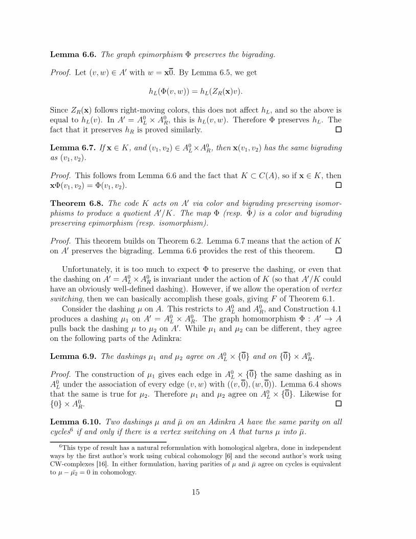
Lemma 6.6. The graph epimorphism Φ preserves the bigrading.

Proof. Let (v, w) ∈ A′ with w = x0. By Lemma 6.5, we get

hL(Φ(v, w)) = hL(ZR(x)v).

Since ZR(x) follows right-moving colors, this does not affect hL, and so the above isequal to hL(v). In A′ = A0

L × A0R, this is hL(v, w). Therefore Φ preserves hL. The

fact that it preserves hR is proved similarly.

Lemma 6.7. If x ∈ K, and (v1, v2) ∈ A0L×A0

R, then x(v1, v2) has the same bigradingas (v1, v2).

Proof. This follows from Lemma 6.6 and the fact that K ⊂ C(A), so if x ∈ K, thenxΦ(v1, v2) = Φ(v1, v2).

Theorem 6.8. The code K acts on A′ via color and bigrading preserving isomor-phisms to produce a quotient A′/K. The map Φ (resp. Φ) is a color and bigradingpreserving epimorphism (resp. isomorphism).

Proof. This theorem builds on Theorem 6.2. Lemma 6.7 means that the action of Kon A′ preserves the bigrading. Lemma 6.6 provides the rest of this theorem.

Unfortunately, it is too much to expect Φ to preserve the dashing, or even thatthe dashing on A′ = A0

L×A0R is invariant under the action of K (so that A′/K could

have an obviously well-defined dashing). However, if we allow the operation of vertexswitching, then we can basically accomplish these goals, giving F of Theorem 6.1.

Consider the dashing µ on A. This restricts to A0L and A0

R, and Construction 4.1produces a dashing µ1 on A′ = A0

L × A0R. The graph homomorphism Φ : A′ → A

pulls back the dashing µ to µ2 on A′. While µ1 and µ2 can be different, they agreeon the following parts of the Adinkra:

Lemma 6.9. The dashings µ1 and µ2 agree on A0L × {0} and on {0} × A0

R.

Proof. The construction of µ1 gives each edge in A0L × {0} the same dashing as in

A0L under the association of every edge (v, w) with ((v, 0), (w, 0)). Lemma 6.4 shows

that the same is true for µ2. Therefore µ1 and µ2 agree on A0L × {0}. Likewise for

{0} ×A0R.

Lemma 6.10. Two dashings µ and µ on an Adinkra A have the same parity on allcycles6 if and only if there is a vertex switching on A that turns µ into µ.

6This type of result has a natural reformulation with homological algebra, done in independentways by the first author’s work using cubical cohomology [6] and the second author’s work usingCW-complexes [16]. In either formulation, having parities of µ and µ agree on cycles is equivalentto µ− µ2 = 0 in cohomology.

15

Proof. Since vertex switching preserves parity on any cycle, the “if” direction is trivialand it suffices to prove the other direction.

Assume µ and µ have the same parity on all cycles. It suffices to prove thestatement for A connected, since we can repeat our argument on each connectedcomponent of A.

Next, we shall prove that for any tree T that is a subgraph of A, there exists avertex switching F on A so that F (µ) and µ agree on T . This can be proved byinduction the number of vertices in T . The base case of one vertex is trivial. If Thas more than one vertex, then there is a leaf v in T incident to only one edge e inT . Let T0 be the tree with the vertex v and edge e omitted. Then T0 has one fewervertex than T so by the inductive hypothesis, there is a vertex switching F0 on A sothat F0(µ) and µ agree on T0. If F0(µ)(e) 6= µ(e), then let F be the vertex switchingF0 followed by a vertex switching at v; otherwise let F = F0. Then F (µ) and F0(µ)agree on T0, so F (µ) agrees with µ on all of T .

Now in the case where T is a spanning tree (so that it is maximal), we claim thatF (µ) and µ agree on all of A. Consider any edge e not in T . This edge completes atleast one cycle with edges in T (otherwise T was not a spanning tree). Since the twocycles have the same parity in F (µ) and µ by assumption, and the F (µ) and µ agreeon all edges in the cycle except for e, they must agree on e as well. Thus, F (µ) = µon all of A.

Now we return to the two dashings µ1 and µ2 on A′. Based on what we justproved, the following lemma will assure the existence of a vertex switching thatsends µ1 to µ2. It uses the fact that these two dashings agree on A0

L × {0} and{0} × A0

R (Lemma 6.9). In terms of the cubical cohomology, this result is a kind ofKünneth theorem.

Lemma 6.11. The parities of µ1 and µ2 agree on all cycles of A′.

Proof. Let our cycle be (v0, v1, . . . , vk) with v0 = vk. We first consider the case wherev0 = 0.

For this proof, we define a color sequence of a path to be the sequence of colors(c(v0, v1), c(v1, v2), . . . , c(vk−1, vk)) of edges along the path. Note that given a startingvertex v0 and a color sequence, there is a unique path that starts at v0 with thatcolor sequence7. This follows by applying induction to Property 2 of the definitionof an Adinkra.

We begin with the color sequence for the cycle (v0, . . . , vk). We will now describea series of modifications to this cycle, described by modifying the color sequence.The idea is to perform a “bubble sort”, by iteratively swapping adjacent colors untilthe left-moving colors are all at the beginning and the right-moving colors are all atthe end.

7Recall in Section 2.2 we treated this sequence of colors as a Zn2

action on the underlying graph,where the order did not matter. In this proof we are not just traversing the graph but also keepingtrack of the sign of the dashings, so we have to keep in mind the order.

16

vj−2 vj−1

vj

vj′

vj+1 vj+2

cj−1

cj cj+1

cj+1 cj

cj+2

Figure 7: An adjacent swap of colors. If we swap colors in position j and j + 1,vertex vj will be replaced by vertex vj

′, and the path gets modified from the upperpath to the lower path in the diagram. The parity of the path changes by exactly 1modulo 2 because the square above has odd parity.

First, given a color sequence

(c1, . . . , cj−1, cj, cj+1, cj+2, . . . , ck),

an adjacent swap results in a color sequence

(c1, . . . , cj−1, cj+1, cj, cj+2, . . . , ck).

Modifying a color sequence in this way leads to a new path from 0. The pathis unchanged up to vj−1, but by the definition of Adinkras, property 2, the pathreturns to vj+1 so it is only vj that has changed (see Figure 7). Thus, the new pathis still a cycle starting at 0. The effect on the parity of any dashing is, by property3, to add 1 modulo 2. In particular, µ1 and µ2 are both affected in the same way.

It is straightforward to find a series of adjacent swaps so that the left-movingcolors are moved to the beginning of the color sequence. Then the resulting pathstarts from 0, stays in A0

L ×{0}, then follows right-moving edges, ending in 0. Sincethe right-moving edges end in 0, it must be that the right-moving edges are in{0} × A0

R. By Lemma 6.9, µ1 and µ2 are equal here, and so their parities on thismodified path are the same. Therefore, their parities on the original loop were thesame.

Now we consider loops p where v0 6= 0. Since A0L × A0

R is connected, there isa path p0 from 0 to v0. Take the path p0, followed by p, then followed by p−1

0

(meaning p0 traversed in the opposite sense). This is a loop starting and ending in0, but the parity of a dashing is the same as that of p, since every new edge in p0 iscounterbalanced by a new edge in p−1

0 . Therefore the parities of µ1 and µ2 agree onall loops.

We are now ready to put everything together and prove our main theorem.

17

Proof of Theorem 6.1. Let A be a connected 2-d Adinkra, and define A0L, A0

R, A′,C ′, K, Φ, and Φ as above.

Use Construction 4.1 to construct the 2-d Adinkra A′ = A0L × A0

R with dashingµ1. By Theorem 6.2 and Theorem 6.8, there is a graph homomorphism Φ : A′ → Athat preserves colors and bigrading. If we take the dashing µ from A and pull it backusing Φ to a dashing µ2 on A′, then Lemma 6.11 and Lemma 6.10 together gives theexistence of a vertex switching F sending µ1 to µ2.

By Theorem 6.8, K acts on A′ to produce A′/K, a well-defined 2-d Adinkrawithout dashing, and an isomorphism Φ : A′/K → A that preserves colors andthe bigrading. Since µ2 is invariant under K, we obtain F (A′)/K, a well-defined2-d Adinkra with dashing. Since F (A′) and A′ only differ in dashing, Φ is still anisomorphism that preserves colors and bigrading. Since µ2 is obtained by pullingback µ from A, this isomorphism preserves dashing as well.

7 The Structure of 2-d Adinkras

Theorem 6.1 is very powerful; we immediately know a lot about what a 2-d Adinkramust look like. Let the support of a 2-d Adinkra (and/or its bigrading function(hL, hR)) be defined as the range of (hL, hR), its bigrading function. Then:

Corollary 7.1. Let A be a connected 2-d Adinkra. The support of A is a rectangle.That is, there exist integers x0, x1, y0, and y1 such that the support is

{(i, j) ∈ Z2 | x0 ≤ i ≤ x1 and y0 ≤ j ≤ y1}.

Proof. Since A0L is a connected 1-d Adinkra and edges change hL by 1, there are

integers x0 and x1 so that the range of the grading is {i | x0 ≤ i ≤ x1}. Likewise A0R

has a range of grading {j | y0 ≤ j ≤ y1} for some integers y0 and y1.By Construction 4.1, the support of A′ = A0

L × A0R is

{(i, j) | x0 ≤ i ≤ x1 and y0 ≤ j ≤ y1}.

Since Φ preserves the bigrading, this is the support of A as well.

Proposition 7.2. Let A be a connected 2-d Adinkra. All connected components ofAL (and respectively AR) are isomorphic as graded posets.

Proof. Consider a connected component of AL. Suppose v is a vertex in this con-nected component. Then there is a x ∈ Zn

2 so that x0 = v. Then the mapf : AL → AL with f(w) = x(w) is a color-preserving graph isomorphism. Thus,it sends connected components onto connected components, and in particular, A0

L tothe connected component containing v.

From these results and the results of the previous section, we now fully knowwhat a 2-d Adinkra looks like. All of the graphical data of a 2-d Adinkra is basicallydictated by the connected components (one from left-moving colors and one fromright-moving colors) of any single vertex and how they are glued together (this iswhat K encodes); then these “slices” are put together into a rectangle.

18

7.1 Constructing 2-d Adinkras

An alternate way to view Theorem 6.1 is as a way to construct all 2-d Adinkras.

Construction 7.3. First choose any doubly-even code and any codeword in itsorthogonal complement. Theorem 5.11 shows this is exactly the amount of data weneed to create an ESDC code C. Write

C = CL ⊕ CR ⊕K,

where CL = C∩ZL(Zp2) and CR = C∩ZR(Z

q2). Use the quotient construction involved

in Theorem 2.3 to create the 1-d Adinkras A1 = Ip/πL(CL) and A2 = Iq/πR(CR),where πL : Zn

2 → Zp2 is projection onto the first p bits and πR : Zn

2 → Zq2 is projection

onto the last q bits.

Second, we need a grading h1 on A1 that is invariant under πL(K) and a gradingh2 on A2 that is invariant under πR(K). There are a finite number of rank functionsto consider for each graph, so it is definitely possible in principle to generate allgradings8 though this is expected to be a large set for higher n. Construct thequotient A = (A1 × A2)/K using Construction 4.1. This produces a graph withcolors and a bigrading. The invariance of the gradings h1 and h2 makes this bi-grading well-defined under the quotient.

Finally, we put an admissible dashing on A. There is again a finite number ofpossible dashings, so this doable via an exhaustive process. We can obtain dashingson the 1-d Adinkra In/C and use Φ to pull them back to A. Recall the discussionafter Theorem 2.3 for relevant results.

Theorem 7.4. Every 2-d Adinkra can obtained by this construction.

Proof. Given any 2-d Adinkra A, there is an ESDC code C. Pick a vertex 0 anddefine A0

L and A0R as in (6.1).

Restrict the gradings hL and hR onto A0L and A0

R. Note that if g ∈ C, thenπL(g)v = πR(g)v, and so hL(πL(g)v) = hL(v) and hR(πL(g)v) = hR(v). ThereforehL restricted to A0

L is invariant under πL(K). Likewise hR restricted to A0R is invari-

ant under πR(K). The dashings, as described in [5], can be obtained by choosingthe specific quotient In/C. Theorem 6.1 gives a description of A in terms of thisconstruction.

Example 7.5. Consider the code given by the generating matrix/vector[

1 1 1 1]

.Then CL and CR are trivial, with p = q = 2, and K is generated by

[

1 1 1 1]

.

As graphs, the Adinkras A1 and A2 are both isomorphic to I2. There are normally2 ways (up to relabeling of vertices) to put a rank function on I2:

8For specific algorithms, one can use either the “hanging gardens” construction in Ref. [2] orconsider the vertices of the “rank family poset” from [16].

19

1

2

3h

However, the height function must be invariant under πL(C) = πR(C) = 〈11〉. Inother words, moving once with an edge of both colors should not change the grading.Thus, both A1 and A2 can only be graded via the rank function depicted on theright. So they must look like this, after assigning colors:

We now take the product A1 × A2, which has 4× 4 = 16 vertices:

To construct A1×A2/K, recall that K is generated by[

1 1 1 1]

, which meansthat each vertex is identified with the vertex that is obtained by following all fourcolors once. We should now get a graph with 16/2 = 8 vertices. If we put anadmissible dashing on it, we obtain a complete 2-d Adinkra. One such choice recoversour Adinkra from Figure 4:

20

8 Conclusion and Future Work

In this work, we have continued in the vein of [13] to study 2-d Adinkras and pro-vided stuctural results to study them combinatorially. Describing already-knownworldsheet supermultiplets in these terms could lead to new insights about thesesupermultiplets, and lead to the discovery of new worldsheet supermultiplets.

One of the motivations for [8] was the idea of studying 4-dimensional or higher-dimensional supermultiplets dimensionally reduced to 1 dimension. Likewise, thepresent work allows us to study the dimensional reduction to 2 dimensions, whichmight carry important information about the original supermultiplet.

As in [14], we could also consider non-adinkraic worldsheet supermultiplets. Itwould be interesting to see if, as in the case of one dimension, there is a continuumof worldsheet supermultiplets. Another direction to extend these results is localsupersymmetry, as in the case of supergravity or superconformal theories, whichcould be of importance to superstrings.

Of course, one obvious step is to go to three or four dimensions. It is expected thatSO(1, d − 1) representations will play a role, and this work may begin to intersect[9, 10].9 Beyond this, it is hoped that this work will generally help develop ourknowledge of supersymmetry in two dimensions.

Many mathematicians may appreciate Adinkras simply as nice combinatorial ob-jects with lots of structure, with surprising links to coding theory, switching graphs,and graph coloring. This view presents additional questions, less relevant to thephysics but still mathematically interesting, in the spirit of Theorem 5.11:

• For example, it would be good to know how many ESDE’s are “compatible” witha 1-d Adinkra A (i.e. there is some 2-d Adinkra A′ with the same underlyinggraph and rankings as A, with the required ESDE as its code), or with thefamily of 1-d Adinkras with the same underlying graph.

• Enumerating all 2-d Adinkras is also a natural goal, though fairly ambitious10,but counting all 2-d Adinkras under some natural constraints may be fruitful.

• How often does the main theorem require no additional vertex switching (i.e. Fis the identity)? In general, when given a dashing, we can ask related questionsabout the minimum number of vertex switches needed to produce a dashingwith a well-defined quotient.

9Higher dimensions is also a natural place to consider gauge fields, which have not yet played arole in this discussion. In one dimension gauge fields can be gauged away to zero. In two dimensionsthis is not the case, but the corresponding field strengths automatically satisfy Bianchi identities,and so the Adinkra formalism works well in this case. But in higher dimensions, gauge fields willbe more difficult to avoid.

10We still do not know how to count 1-d Adinkras with In as underlying graph beyond small n.For In/C with nontrivial C, we have almost no data! The work in [16] basically settles dashingscompletely and gives some structural results on rankings, but counting rankings completely remainsa very difficult problem, related to the chromatic polynomial for some families of C.

21

Acknowledgments

The authors wish to thank Charles Doran, Sylvester Gates, and Tristan Hübsch forhelpful conversation.

A Relation to Hübsch’s Original Language

The statement of Theorem 6.1 is a bit different from the statement of the conjecturein [13]. There, the language was partly in terms of representations of the 2-d SUSYalgebra instead of graphs.

Construction A.1 (Construction 2.1 (off-shell)). Let R+ and R− denote off-shellrepresentations of two copies of the 1-d SUSY algebra with p and q colors, respec-tively, and let Z be a symmetry of R+ ⊗ R−, as a representation. The Z-quotientof the tensor product (R+ ⊗ R−)/Z is then an off-shell representation of 2-d SUSYalgebra with (p, q) colors.

The conjecture in [13] then says that every Adinkraic representation of 2-d SUSYwith (p, q) colors is obtained by this construction.

The relation between this conjecture and Theorem 6.1 will be apparent once weestablish the following relationships. None of these facts are new to this paper, butthis information is collected here for the convenience of the reader.

• The relationship between off-shell representations of SUSY and Adinkras: Thisis the central idea behind the original paper on Adinkras[8], and so we do notgo into detail here. The idea is that each vertex v of the Adinkra correspondsto a field fv in the SUSY representation, and Qi acts on fields by the edgeof color i, with possible derivatives depending on the grading or bigrading (asthe case may be), and with an extra minus sign if the corresponding edge isdashed.

• The relationship between A1 × A2 and R+ ⊗ R−: The definition of R+ ⊗ R−

as a representation of 2-d SUSY that

Qi(fv ⊗ fw) = Qi(fv)⊗ fw

if i ≤ p andQi(fv ⊗ fw) = (−1)|h(v)|fv ⊗Qi(fw)

if i > p. This is the standard way in which tensor products are defined inZ2-graded algebras.[1, 11] Then Construction 4.1 mimics this definition on thelevel of Adinkras.

• A vertex switching at v corresponds to replacing fv with −fv. Then all equa-tions involving Qi(fv) or fv will get an extra minus sign. This reverses alldashings on edges connected to v.

• A quotient defined in Theorem 6.1 is a symmetry Z of the representation.

22

References

[1] R. Bott and L. W. Tu. Differential forms in algebraic topology, volume 82 ofGraduate Texts in Mathematics. Springer-Verlag, New York, 1982.

[2] C. F. Doran, M. G. Faux, S. J. Gates Jr., T. Hübsch, K. Iga, and G. D. Landwe-ber. On graph-theoretic identifications of Adinkras, supersymmetry representa-tions and superfields. International Journal of Modern Physics, 22(5):869–930,2007.

[3] C. F. Doran, M. G. Faux, S. J. Gates Jr., T. Hübsch, K. Iga, and G. D. Landwe-ber. Relating Doubly-Even Error-Correcting Codes, Graphs, and IrreducibleRepresentations of N-Extended Supersymmetry. Discrete and ComputationalMathematics, 2008.

[4] C. F. Doran, M. G. Faux, S. J. Gates Jr., T. Hübsch, K. Iga, G. D. Landweber,and R. Miller. Codes and Supersymmetry in One Dimension. Adv. Theor. Math.Phys., 15:1909–1970, 2011.

[5] C. F. Doran, M. G. Faux, S. J. Gates Jr., T. Hübsch, K. Iga, G. D. Landweber,and R. L. Miller. Topology types of Adinkras and the corresponding represen-tations of N-extended supersymmetry. arXiv:0806.0050, 2008.

[6] C. F. Doran, K. Iga, and G. D. Landweber. An application of Cubical Coho-mology to Adinkras and Supersymmetry Representations. arXiv:1207.6806,2012.

[7] B. L. Douglas, S. J. Gates Jr., B. L. Segler, and J. Wang. AutomorphismProperties and Classification of Adinkras. Advances in Mathematical Physics,accepted.

[8] M. G. Faux and S. J. Gates Jr. Adinkras: A graphical technology for supersym-metric representation theory. Physical Review D, 71(6), 2005.

[9] M. G. Faux, K. Iga, and G. D. Landweber. Dimensional enhancement viasupersymmetry, July 2011.

[10] M. G. Faux and G. D. Landweber. Spin holography via dimensional enhance-ment. Physics Letters B, 681:161–165, Oct. 2009.

[11] D. Freed. Five lectures on supersymmetry. American Mathematical Society,Providence, RI, 1999.

[12] S. J. Gates Jr. and T. Hübsch. On Dimensional Extension of Supersymmetry:From Worldlines to Worldsheets. Adv. in Th. Math. Phys., 16:1619–1667, 2012.

[13] T. Hübsch. Weaving Worldsheet Supermultiplets from the Worldlines Within.Adv. in Th. Math. Phys., 17:1–72, 2013.

23

[14] T. Hübsch and G. A. Katona. A q-continuum of off-shell supermultiplets.arXiv:1310.3256, 2013.

[15] J. J. Seidel. A survey of two-graphs. In Colloquio Internazionale sulle TeorieCombinatorie (Rome, 1973), Tomo I, pages 481—-511. Atti dei Convegni Lincei,No. 17. Accad. Naz. Lincei, Rome, 1976.

[16] Y. X. Zhang. Adinkras for mathematicians. Transactions of the AmericanMathematical Society, 366(6):3325–3355, 2014.

24