Structural Dynamics Teaching Example - A Linear Test Analysis Case Using Open Software

Per-Olof Sturesson, PhD

Noise & Vibration Center, Volvo Car Corporation, Dept. 91600/PV2C, SE-405 31 Gothenburg, Sweden

Anders Brandt, Associate Professor

Inst. of Technology and Innovation, University of Southern Denmark, Campusvej 55, DK-5230 Odense M, Denmark

Matti Ristinmaa, Professor

Division of Solid Mechanics, Lund University, P.O. Box 124, SE-221 00 Lund, Sweden

NOMENCLATURE h(t) Impulse response function H(f) Frequency response function [L] Modal participation matrix N Number of degrees-of-freedom {ψ}r Mode shape of mode number r sr Pole of mode number r u, v, w Displacement [a] Nodal displacement [K] Global stiffness matrix [M] Global mass matrix [k]e Element stiffness matrix [m]e Element mass matrix [F] Body force matrix strain stress E Young’s modulus Poisson’s ratio [N] Shape function matrix Mass density t Material thickness

ABSTRACT Teaching the topic of structural dynamics in any engineering field is a true challenge due to the wide span of the underlying subjects like mathematics, mechanics (both rigid body and continuum mechanics), numerical analysis, random data analysis and physical understanding. With the increased availability of computers many engineering problems in practice are evaluated by means of numerical methods. The teaching task within the field of structural dynamics thus has to include analytical models in order to create a theoretical basis but also has to include computational techniques with its approximations, and knowledge about their limitations. Equally important is for students to have knowledge of the experimental verification of the obtained models. This paper describes a teaching example where a simple plate structure is modeled by shell elements, followed by a model calibration using experimental modal analysis data. By using open software, based on MATLAB®1 as a basis for the example, the applied numerical methods are made transparent to the student. The example is built on a combination of the free CALFEM®2 and ABRAVIBE toolboxes, and thus all code used in this paper is publically available as open source code.

Keywords: Experimental modal analysis, finite element model, model calibration, ABRAVIBE, CALFEM

INTRODUCTION For transparency in teaching it is advantageous to provide students with a simple case, so that focus can be put on the theory and techniques taught, rather than object related problems. In addition, open source software based on MATLAB® or GNU Octave, provides the advantage that the students can follow each step in the process, with direct access to governing equations and variables involved. This transparency is not usually possible with commercial finite element programs. In commercial codes some of these teaching concepts are lost since many of the problems can, in fact, be solved without understanding the underlying physics and numerical methods and their limitations.

The aim of CALFEM® [1] was to highlight the link between the mathematical theory and models of a phenomena and its numerical implementation using the finite element method. In such an approach the students are motivated to fully appreciate the intimate relationship between these topics. Also within such an approach it becomes evident for the students that many different physical problems are in fact modeled by the same set of equations, i.e. analogies exist. An additional advantage of open-source code is that the student can also copy a routine and modify it for a specific purpose such as modeling of some special damping.

Model calibration, or correlation theory and methods, are important subjects to teach engineering students. The theory is becoming more and more important for many OEMs who require an efficient and streamlined product development process that enables getting products faster to the market. This is especially important in highly competitive sectors like the automotive industry. Additional efficiency, i.e. cost reduction in product development, may be achieved by means of reducing both the number of prototype build stages and the number of prototypes within a given build stage. Without taking correct countermeasures it is evident that this increases the risk of product quality issues in the field due to errors in the early decision making process.

In order to minimize the risks different actions need to be applied long before hardware builds take place, i.e. before and during the early phase of the product development. These “front loading” actions usually include extensive use of computer aided technologies like CAE in order to enable improved project decision making based on objective data as well as engineering insight but also, which is as important, a more robust process for target setting including subsystem target roll down. A successful outcome of these actions depends heavily on the capability of the applied math methods. The development of new or improving existing math methods is then an important and strategic task that needs to be done outside and upfront to the regular product development work. This task also requires test and CAE communities to thoroughly co-operate in order to be successful. Often organisation and conflicting priorities may be difficult barriers to overcome. Also important in math method development is to address the issue of access to hardware that matches the design. Variability due to manufacturing processes affects the hardware testing and needs also to be considered.

For transparency in teaching it can be an advantage to provide students with a simple case, so that focus can be put on the theory and techniques taught, rather than object related problems. In addition, open source software based on MATLAB®, provides the advantage that the students can follow each step in the process, with direct access to governing equations and

1 MATLAB® is a trademark of The MathWorks, Inc. 2 CALFEM® is a trademark of the Division of Structural Mechanics, Lund University.

variables involved. Therefore, in this paper we describe an example of a FE model of a simple PMMA plate, similar to the so-called IES plate [2], made in the popular CALFEM® open-source MATLAB® toolbox. Experimental modal analysis is then performed and correlation analysis and simple model calibration is performed. For the experimental modal analysis we use the open source ABRAVIBE toolbox, also for MATLAB®. If fully free, open source software is wanted, all examples can also be run in GNU Octave, using the same toolboxes.

THEORY

Experimental Modal Analysis (EMA)

Experimental modal analysis is based on measurements of frequency response functions from which the modal parameters (natural frequencies, relative damping ratios, and mode shapes) are extracted using the relation

* * *

*1 j j

TTN

rr r r r r

r r r

QQH f

s s

(1)

where H f is the matrix of frequency responses in receptance form (displacement/force), r

Q is the modal scaling

constant, rs the pole of mode number r , r

the mode shape for mode number r , and N is the number of modes

(number of degrees-of-freedom). In the typical case, a few, say R , references are used, either using fixed shakers and roving response sensors (usually accelerometers) which leads to estimates of R columns from the matrix in Eq. (1), or by letting R reference accelerometers be fixed and roving the force around, usually with an impact hammer, which leads to estimates of R rows of Eq. (1). In any case, since the frequency response matrix is symmetric, it can easily be transposed if the latter strategy was chosen, so that the formulation may be implemented only for the case of fixed force references.

Instead of the frequency domain relation in Eq. (1), time domain methods extract the modal parameters by using the relation

of the impulse responses in a matrix h t , which can be expressed

** * *

1

r r

N TT s t s tr rr r r r

r

h t Q e Q e

. (2)

If two or more poles are very close, several references usually have to be used to correctly extract the corresponding mode shapes. Also, many times the complex conjugate poles and mode shapes are, for simplicity, included in the numbering, so that the sums go from 1 to 2N and only include one term. Eq. (2) can then be rewritten as

rs th t e L (3)

where is the mode shape matrix with mode shapes in its columns, rs te is a diagonal matrix with the complex

exponential terms, and L is a matrix with modal participation factors.

A common family of parameter extraction methods for extracting poles are the complex exponential methods; the prony method [3], the least squares complex exponential method [4], and the polyreference time domain method [5]. The latter method can handle closely coupled poles. In all cases, the mode shapes are usually computed in a second step, e.g. by the least squares frequency domain method [6]. These methods are all implemented in the ABRAVIBE toolbox [7].

Finite Element Method

The finite element method for solving structural dynamic problems is today well established in the industry. More comprehensive reading concerning formulation and basic theory of finite element method can be found in [8-10] while structural dynamic theory can be found in [11].

If an arbitrary linear elastic structure or medium is considered, the equations that describe the dynamic response may be derived by the equilibrium of the work carried out by the external forces acting on structure and the work of the internal, inertial and viscous forces. For a single finite element the work balance yields [8-10]

1

e e

e e e

NT T T

i iiV S

T T T

V V V

u F dV u dS u p

dV u u dV u c u dV

(4)

where u and are virtual displacements and corresponding strains, F the body forces, the prescribed

surface tractions, ip the concentrated point loads with dimension n, the mass density of the material and c is the

viscous material damping parameter.

The variables to be solved in structural mechanics using the finite element approach are usually the displacement field u

u

u v

w

(5)

where u, v and w are the displacements in x, y and z-direction using a Cartesian coordinate system. The kinematic relationship between strains and displacement is defined as

u (6)

where

0 0

0 0

0 0

,0

0

0

x

y

z

xy

xz

yz

x

y

z

y x

z x

z y

(7)

By introducing shape functions N the displacement field u and its two time derivatives yields

u N a

u N a

u N a

(8)

where the shape functions are space dependent only and the nodal deformations a are dependent of time (or frequency)

only. The strains at the nodal degrees of freedom may be derived as

u N a B a . (9)

By combining Eq. (4) and Eq. (8) we get

1e e

e e e

NT TT

iiV S

T T TT

V V V

a N F dV N dS p

a B dV N N dV a c N N dV a

.

(10)

Since a is arbitrary Eq.(10) can be written as

int texe em a c a f f (11)

where the element mass and viscous damping matrices are

e

T

eV

m N N dV (12)

e

T

eV

c c N N dV (13)

and the element internal and external force vectors are defined as

int

e

T

V

f B dV (14)

1

e e

NT T

ext iiV S

f N F dV N dS p

.

(15)

In the demonstration example first order shell elements will be used. The shell element consists of combination of a continuous plane stress (2D) element, which describe the membrane behaviour, and a structural plate element, which describe the bending behaviour. Plate theory implies several simplifications and also violations of the fulfilment of solid mechanic field equations. Nevertheless, shell elements are widely used in industry due to less effort in modelling and computational efficiency.

For the membrane behaviour of the shell element, i.e. described by a plane stress element, the following constitutive relation between stress and strain exists [8-10]

2

1 0

1 01

10 0

2

x x

y y

xy xy

ED

(16)

where E is the Young’s modulus and Poisson’s ratio, respectively. The shape functions for a rectangular four node plane stress element, which has eight degrees of freedom, is

1 2 3 4

1 2 3 4

0 0 0 0

0 0 0 0

N N N NN

N N N N

(17)

where

( )( )i i i iN b x c y d (18)

where b, c and d are constants. By using Eq. (9), (14) and (16) the element stiffness matrix can be derived as

e

T

eV

K B D B dV (19)

which is a eight-by-eight matrix in case of a four node plane stress element. For consistency it should be mentioned that in the two-dimensional formulations all rows and columns in Eq. (7) referring to variables in z-direction are condensated.

The bending behaviour of the shell element is as mentioned before described by plate theory. More background reading can be found in [12]. In general, a plate is defined as a structure with a thickness t that is small compared with all other dimensions of the plate. Also, loading occurs only in the direction normal to the plate. In this article Kirchhoff (thin) plate theory is used for finite element implementation. The element stiffness matrix for a plate finite element yields a different formulation compared to a plane stress element. In order to derive the plate element stiffness formulation statics is used for simplicity. The deflection w in the normal direction of the plate is given by the biharmonic equation

4 4 4 2

4 2 2 4 3

12(1 )2

w w wq

x x y y Et

(20)

where w is the displacement in the normal direction of the plate (z-direction) and q the unit load per surface area or using the bending moment as variable

2 22

2 22 0xy yyxx

M MMq

x x y y

(21)

using

3

ˆ12

tM D w (22)

and

2

2

2

2

2

ˆ,

2

xx

yy

xy

xM

M My

M

x y

.

(23)

The displacement field u for a plate finite element consists of, in addition to w, two rotational degrees of freedom

w

u w x

w y

(24)

The deformation or rotation at any arbitrary point in the element is given by

u N a (25)

where a contains the nodal displacement or rotations. Each node has three deformation degrees of freedom, one

displacement and two rotations.

The shape function matrix for all degrees of freedom in a rectangular plate element is given by

1 4 7 10

2 5 8 11

3 6 9 12

0 0 0 0 0 0 0 0

0 0 0 0 0 0 0 0

0 0 0 0 0 0 0 0

N N N N

N N N N N

N N N N

(26)

The shape function iN is given by the field function;

2 2 2 20 1 2 3 4 5 6 7

3 3 3 38 9 10 11

( , )x y c c x c y c x c y c xy c x y c xy

c x c y c x y c xy

(27)

or

( , )x y x c (28)

where

2 2 2 2 3 3 3 31x x y x y xy x y xy x y x y xy (29)

and

0 1 2 3 4 5 6 7 8 9 10 11

Tc c c c c c c c c c c c c

. (30)

By means of Hermitian interpolation of each shape function iN the coefficients ic are given by the boundary conditions in

terms of ordinates and slopes at each element nodal point.

The derivation of the finite element formulation for the plate element stiffness matrix is more complex than for the plain stress element. For a more comprehensive derivation the reader can read [8-10]. Using Eq.(21) and deriving its weak form it yields

( )e e e e

T T T Tnmnn nz

A S S A

dMB M dA N n M dS N V dS N q dA

dm (31)

where

ˆB N (32)

and nzV and nmM are the applied forces and moments at the plate element boundary.

The right hand side terms contain the kinematic and static boundary conditions as well as the loads due to body forces. By using Eq.(22) and the left hand side term of Eq. (31) the 12x12 plate element stiffness matrix yields

ˆ ˆ

e

T

eA

K B D B dA (33)

where

3

12

tD D (34)

In this example the shell element formulation has five nodal degrees of freedom. It should be mentioned that in many commercial finite element packages the shell element formulations use six nodal degrees of freedom. The sixth degree of freedom, often referred as “the drilling DOF”, is needed when curved shapes are analyzed.

By means of assembling the element mass and stiffness matrices for each finite element using the model topology the system equations may be derived. Assuming no loads the free vibration equation of motion yields [11]

0M a K a (35)

and by assuming harmonic motion for each degree of freedom iu

sini iu u t (36)

where iu is the amplitude, then Eq.(35) yields the eigenvalue problem

2 0M K a . (37)

In the current release of the CALFEM® toolbox [13] no finite element formulation for shell element is directly implemented. However, as mentioned earlier the finite element formulation for shell elements is a combination of membrane and plate elements. Both these two finite element formulations are implemented for static analysis. Functions for element mass matrix

formulation for shell element has therefore been developed for this demonstration example together with dynamic model check function like mass calculation by means of evaluation of the global mass matrix.

Model Verification

There are two common methods to verify an FE model, either using natural frequencies and mode shapes, or using frequency responses [14]. In this paper we will use the latter method. The first comparison is usually to match frequencies of each mode in the FE model with the corresponding mode in the experimental results. For this comparison, the MAC (modal assurance criterion) matrix [15] is used to determine which of the mode in one set should be paired with which mode in the other set. The MAC value between two modes r and s , is defined by

2

MAC ,

T

r s

T T

r r s s

r s

(38)

and is similar to the correlation coefficient of the two vectors. For best comparison between test and analytical model, a good EMA test for verification purposes should use sensor positions that minimize the off-diagonal components in the MAC matrix.

After pairing the mode shapes, and comparing the natural frequencies of the EMA results with the eigenfrequencies of the FE model, the FE model should be modified so that eigenfrequencies match the experimental model, within some accuracy limits or if test errors are evident the test sequence should be reworked. Recommended criteria for a verified FE model is that the eigenfrequencies for most important modes lies within 2-10% and the diagonal elements of the MAC matrix are greater than 0.9 and off-diagonal elements are less than 0.1 [14]. For simple structures, like the example used in this article the upper limit of frequency criteria should be less than 5% and the diagonal elements of the MAC matrix should be greater than 0.95. In practice for complex engineering FE models using too stringent correlation criteria provides limited additional benefits but adds time and cost.

Before adjusting any model parameter it is essential to perform an uncertainty assessment of critical parameters. For sheet metal designed structures, especially stamped, the sheet thickness is non-uniform due to the manufacturing process. Properties of joints, e.g. spot welds or glue, are also candidate parameters to be adjusted. Material properties like Young’s modulus and Poisson’s ratio are well-known for most metallic materials while for complex structures of polymers, where manufacturing process parameters are strongly influencing the material properties, a greater uncertainty exists [18, 19]. In this simple example, parameters to be adjusted are the material properties like the Young’s modulus used in the FE model.

More advanced verification could then be done. To find local errors in the FE model, the cross-orthogonality matrix (see [14]) can be used. This requires computing a reduced mass matrix, and will not be done in the current example. The CoMAC (coordinate MAC) [16] can also be used for this purpose. This measure is defined for each DOF q , by

2

exp ,1

2 2exp ,

1 1

( )( )

( ) ( )

N

qr fe fe qrr

q N N

qr fe fe qrr r

C

(39)

i.e. a summation of the correlation coefficients of each DOF over all modes. A CoMAC value different from unity reveals a DOF where there is discrepancy between the FE model mode shapes and the experimental mode shapes. This could, of course, be due to problems in the FE model in which, sometimes, local stiffness of the structure can be hard to model correctly. A low CoMAC value can, however, also be due to a local error in the EMA result, so great care need to be taken when interpreting local discrepancies.

APPLICATION

Finite Element Model

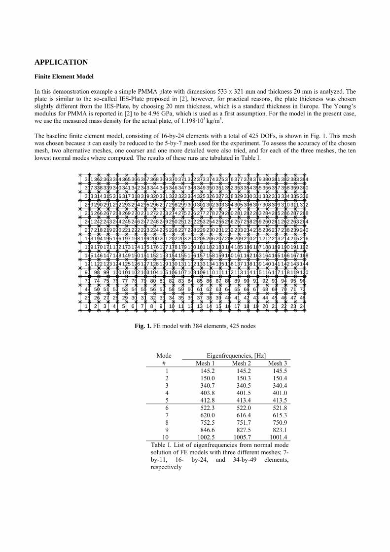
In this demonstration example a simple PMMA plate with dimensions 533 x 321 mm and thickness 20 mm is analyzed. The plate is similar to the so-called IES-Plate proposed in [2], however, for practical reasons, the plate thickness was chosen slightly different from the IES-Plate, by choosing 20 mm thickness, which is a standard thickness in Europe. The Young’s modulus for PMMA is reported in [2] to be 4.96 GPa, which is used as a first assumption. For the model in the present case, we use the measured mass density for the actual plate, of 1.198·103 kg/m3.

The baseline finite element model, consisting of 16-by-24 elements with a total of 425 DOFs, is shown in Fig. 1. This mesh was chosen because it can easily be reduced to the 5-by-7 mesh used for the experiment. To assess the accuracy of the chosen mesh, two alternative meshes, one coarser and one more detailed were also tried, and for each of the three meshes, the ten lowest normal modes where computed. The results of these runs are tabulated in Table I.

Fig. 1. FE model with 384 elements, 425 nodes

Mode

Eigenfrequencies, [Hz]

# Mesh 1 Mesh 2 Mesh 3 1 145.2 145.2 145.5 2 150.0 150.3 150.4 3 340.7 340.5 340.4 4 403.8 401.5 401.0 5 412.8 413.4 413.5 6 522.3 522.0 521.8 7 620.0 616.4 615.3 8 752.5 751.7 750.9 9 846.6 827.5 823.1 10 1002.5 1005.7 1001.4

Table I. List of eigenfrequencies from normal mode solution of FE models with three different meshes; 7-by-11, 16- by-24, and 34-by-49 elements, respectively

1 2 3 4 5 6 7 8 9 10 11 12 13 14 15 16 17 18 19 20 21 22 23 24

25 26 27 28 29 30 31 32 33 34 35 36 37 38 39 40 41 42 43 44 45 46 47 48

49 50 51 52 53 54 55 56 57 58 59 60 61 62 63 64 65 66 67 68 69 70 71 72

73 74 75 76 77 78 79 80 81 82 83 84 85 86 87 88 89 90 91 92 93 94 95 96

97 98 99 100 101 102 103 104 105 106 107 108 109 110 111 112 113 114 115 116 117 118 119 120

121 122 123 124 125 126 127 128 129 130 131 132 133 134 135 136 137 138 139 140 141 142 143 144

145 146 147 148 149 150 151 152 153 154 155 156 157 158 159 160 161 162 163 164 165 166 167 168

169 170 171 172 173 174 175 176 177 178 179 180 181 182 183 184 185 186 187 188 189 190 191 192

193 194 195 196 197 198 199 200 201 202 203 204 205 206 207 208 209 210 211 212 213 214 215 216

217 218 219 220 221 222 223 224 225 226 227 228 229 230 231 232 233 234 235 236 237 238 239 240

241 242 243 244 245 246 247 248 249 250 251 252 253 254 255 256 257 258 259 260 261 262 263 264

265 266 267 268 269 270 271 272 273 274 275 276 277 278 279 280 281 282 283 284 285 286 287 288

289 290 291 292 293 294 295 296 297 298 299 300 301 302 303 304 305 306 307 308 309 310 311 312

313 314 315 316 317 318 319 320 321 322 323 324 325 326 327 328 329 330 331 332 333 334 335 336

337 338 339 340 341 342 343 344 345 346 347 348 349 350 351 352 353 354 355 356 357 358 359 360

361 362 363 364 365 366 367 368 369 370 371 372 373 374 375 376 377 378 379 380 381 382 383 384

The results in Table I show that there is some increased stiffness for the coarser models, resulting in slightly higher eigenfrequencies. The middle grid density seems reasonable, however, so we decided to use this model.

In CALFEM the following steps were implemented in this demonstration example

1. Generate geometrical topology (nodes). 2. Generate element to nodal degree of freedom topology. 3. For each element calculate mass and stiffness matrices and assemble the data into global matrices. 4. Solve the set of equations (eigenvalue extraction). 5. Post process the results.

RESULTS - SIMPLE PLATE

FE Results

The first ten eigenfrequencies from a normal mode solution of the FE model with the mid grid density in Table I are shown in Table II, together with the corresponding values from the EMA test. For the sake of simplicity, the modes are arranged in the order of the experimental modal analysis. Thus the first two FE modes have been swapped, as they appeared in the opposite order. This may be due to the fact that the shell element formulation yields too high bending stiffness. Application of more advanced plate theory could address this.

Mode # FE Eigenfreq. Exp. Natural Freq. [Hz]

Diff. [%]

Damping [%]

Mode Description

1 150.3 145.2 3.4 3.21 First torsion 2 145.3 147.0 -1.1 3.02 First bending, x 3 340.5 332.4 2.4 2.75 Second torsion 4 401.5 409.4 -2.0 2.50 Second bending, x 5 413.4 421.4 -1.9 2.42 First bending, y 6 522.0 518.8 0.6 2.34 Higher-order 7 616.4 608.3 1.3 2.33 Higher-order 8 751.7 745.4 0.8 2.27 Higher-order 9 827.5 830.9 -0.4 2.13 Third bending, x 10 1005.7 992.9 1.3 2.11 Higher-order Table II. Finite element eigenfrequencies, experimentally obtained undamped natural frequencies and relative damping coefficients from experimental modal analysis of PMMA plate, and relative difference between frequencies.

EMA Results

Experimental modal analysis was conducted by impact excitation, using two reference accelerometers in two corners along one of the long axes of the plate. A 7-by-5 grid was used for the measurements. The structure was suspended using soft rubber cords which yielded rigid body modes below 5 Hz. Time domain signals were recorded and processed as described in [15, 17] . Shaker excitation is an alternative that could be used with similar results. An advantage with the PMMA plate for teaching purposes is that it is relatively easy to measure with good accuracy.

The polyreference time domain method [5] was used for estimating the poles, followed by a computation of the mode shapes using the frequency domain least squares method, in both cases using available functions in the ABRAVIBE toolbox. The results of the experimental modal analysis are shown in Table II, where the first ten modes are tabulated in the third column. It is relatively easy to successfully obtain at least 20 experimental modes, but for correlation with the FE model it is more realistic to select the ten lowest modes. As follows from Table II, the ten lowest undamped natural frequencies ranges from approximately 145 to 993 Hz. Relative damping ratios ranges from 2.1% to 3.2%, and are tabulated in column five of Table II.

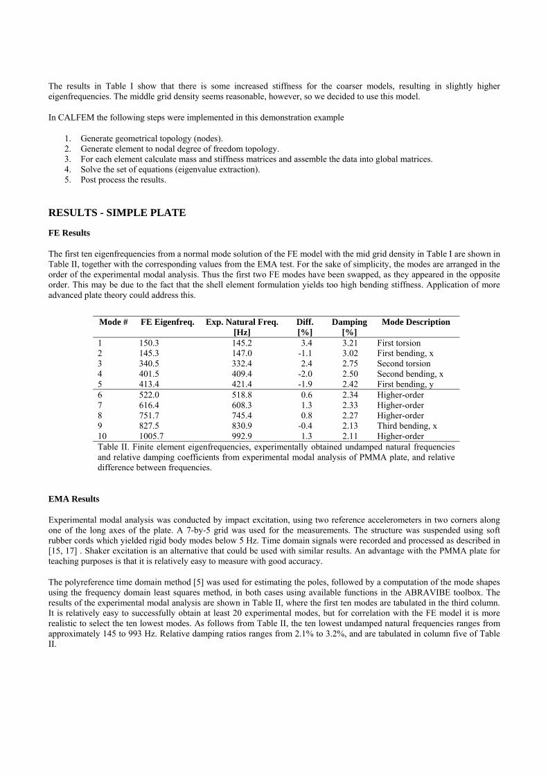
Fig. 2. Cross-MAC matrix between experimental modal analysis mode shapes and normal modes of first FE run

FE Model Calibration

A comparison of the analytical and experimental results in Table II shows that the frequencies are relatively close, and that the two first modes appear in opposite order in the FE model solution compared to the experiment. For comparison with the experimental mode shapes, the mode shapes from the normal mode solution were reduced to every fourth DOF, corresponding to the 5-by-7 grid used for the experiment. A computation of the cross-MAC matrix showed that the mode shapes were very similar, with MAC values in excess of 0.97 except for mode 9 where the MAC matrix was 0.92. A plot of the cross-MAC is shown in Fig. 2.

A simple modification of the FE model is to match the frequency of the first bending mode of the FE model to the corresponding frequency from the experimental results. Since the first bending mode frequency can be assumed to be related to the square root of Young’s modulus, this can be obtained by adjusting the Young’s modulus by the square of the frequency ratio of the two frequencies. From Table I we thus get that the new Young’s modulus should be approx.

24.96 147.0 / 145.3 =5.08 GPa. The FE model was updated with this new Young’s modulus in a second step, and the FE

model was again solved for the first ten eigenfrequencies. The results are shown in Table III, where it can be seen that the first bending mode (mode 2) is within 0.04% of the experimental frequency. The difference for the higher order bending modes, marked by asterisks (*) in the table, are within approx. 1%. The torsion modes, however, are generally slightly overestimated. This is likely a result of the approximations used in the definition of the shell elements used. In our opinion this is good point of the present, simplified exercise, as it gives a reason to discuss the approximations and limitations of various element types.

With the model calibration thus successfully done, the CoMAC values were calculated for all points. The CoMAC values were thus found to be within 0.9 to 1.0 for all modes. There was therefore not found to be any reason to investigate any local

145.2147.0

332.4409.4

421.4518.8

608.3745.4

830.9992.9

150.3145.3

340.5401.5

413.4522.0

616.4751.7

827.51005.7

0

0.2

0.4

0.6

0.8

1

Cross MAC matrix

0.1

0.2

0.3

0.4

0.5

0.6

0.7

0.8

0.9

discrepancies between the experimental and analytical mode shapes in this case, which is rather natural considering the simple structure.

Mode

Natural frequency [Hz]

Difference [%]

# FE Model EMA 1 151.8 145.2 4.37 2 147.0 147.0 0.04* 3 344.0 332.4 3.40 4 406.2 409.4 -0.80* 5 417.0 421.4 -1.06* 6 526.9 518.8 1.52 7 623.0 608.3 2.37 8 759.3 745.4 1.82 9 836.9 830.9 0.71* 10 1016.7 992.9 2.34 Table III. List of eigenfrequencies of FE model after modifying Young’s modulus, and undamped natural frequencies from experimental modal analysis. The bending modes are marked with asterisks (*) for reference. It is seen that the bending modes are relatively well modelled whereas the frequencies of the torsion modes are typically overestimated by the shell elements

CONCLUSIONS The simple test case demonstrates the possibility to teach advanced structural dynamics topics like test-analysis verification using open software. Using open software it is possible to investigate influence of other finite element formulations than in this case a simple shell element with respect to eigenfrequencies and mode shapes. Introduction of pre-test methods using a model reduction scheme like Guyan could also easily be made. Furthermore, the paper discusses some advantages of using a simple structure like the IES plate. The main advantages can be summarized thus:

Using MATLAB (or GNU Octave) makes it possible for the student to look at variables included such as mass and stiffness matrices, mode shapes etc. for deeper insights into the mathematics involved.

The structure is easily modeled to a sufficient accuracy using shell elements, which are computationally inexpensive.

The experimental modal analysis of the plate can be done in a few hours lab time, using either impact testing or shaker testing.

The correlation and updating of the FE model is done very easily and transparently. If more advanced options such as model reduction etc. is wanted, the immediate access to the mass and stiffness

matrices in MATLAB is making the process very easy.

REFERENCES [1] Ristinmaa, M, Sandberg, G., Olsson, K.-G., CALFEM as a Tool for Teaching University Mechanics, International

Journal of Innovation in Science and Mathematics Education, 5, 2000.

[2] Gregory, D., Smallwood, D. Experimental results of the IES Modal Plate, J. of Environmental Sciences, 1989.

[3] Proakis, J. G., Manolakis, D. G., Digital Signal Processing: Principles, Algorithms, and Applications Prentice Hall, 2006.

[4] Brown, D., Allemang, R., Zimmerman, R., Mergeay, M., Parameter Estimation Techniques for Modal Analysis SAE Tech. Papers, 1979.

[5] Vold, H., Kundrat, J., Rocklin, T. G., Russell, R., A Multiple-Input Modal Estimation Algorithm for Mini-Computers, SAE Tech. Papers, 1982.

[6] Maia, N., Silva, J. (Eds.) Theoretical and Experimental Modal Analysis, Research Studies Press, 2003.

[7] A. Brandt, ABRAVIBE, A MATLAB/Octave toolbox for Noise and Vibration Analysis and Teaching, Revision 1.2, 2012. Available from http://www.mathworks.com/matlabcentral/linkexchange/.

[8] Ottosen, N., Petersson, H., Introduction to the Finite Element Method, Prentice Hall, 1992.

[9] Zienkiewicz, O. C., Taylor, R. L., The Finite Element Method – Vol. 2. Solid and Fluid Mechanics, Dynamics and Non-Linearity, Fourth Edition, McGraw Hill, 1991.

[10] Cook, R. D., Malkus, D. S., Plesha, M. E., Concepts and Applications of Finite Element Analysis, Third Edition, John Wiley and Sons, 1989.

[11] Craig Jr, R. R., Kurdila, A. J., Fundamentals of Structural Dynamics, Second Edition, John Wiley and Sons, 2006.

[12] Timosjenko, S. P., Woinowsky-Krieger, S., Theory of Plates and Shells, Second Edition, McGraw-Hill, 1959.

[13] Austrell, P.-E., Dahlblom, O., Lindemann, J., Olsson, A., Olsson, K.-G., Persson, K., Petersson, H., Ristinmaa, M., Sandberg, G., Wernberg P.-A., CALFEM - A Finite Element Toolbox, Version 3.4, KFS i Lund AB, Lund, 2004.

[14] Baker, M., Review of Test/ Analysis Correlation Methods and Criteria for Validation of Finite Element Models For Dynamic Analysis, in: Proc. 10th International Modal Analysis Conference (IMAC), San Diego, CA, 1992.

[15] Brandt, A., Noise and Vibration analysis – Signal Analysis and Experimental Procedures, John Wiley and Sons, 2011.

[16] Lieven, N. A. J., Ewins, D. J., Spatial Correlation of Mode Shapes, The Coordinate Modal Assurance Criterion (CoMAC), Proc. 6th International Modal Analysis Conference (IMAC), Kissimmee, FL, 1988.

[17] Brandt, A., Brincker, R., Impact Excitation Processing for Improved Frequency Response Quality, in: Proc. 28th International Modal Analysis Conference, Jacksonville, FL, 2010.

[18] Chu, J., Saloniemi, E.-L., Consideration to FEM-formulation in Partial Damping Layers for Complex Structures such as Vehicle Floor, Master’s Thesis Report, ISSN 0238-8338, Department of Technical Acoustics, Chalmers University of Technology, 2002.

[19] Weber, J. and Benhayoun, I., Squeak, Rattle Simulation - A Success Enabler in the Development of the New Saab 9-5 Cockpit without Prototype Hardware, SAE Int. J. Passeng. Cars - Mech. Syst. 3(1):936-947, 2010.