Embed Size (px)
Citation preview
Structural characterization ofamorphous materials using x-ray scattering
Todd C. HufnagelDepartment of Materials Science and Engineering
Johns Hopkins University, Baltimore, Maryland
Funding for work on scattering from metallic glasses provided by NSF-DMR, DOE-BES, ARO, ARLScattering data presented collected at SSRL (7-2, 10-2), APS (1-ID), NSLS (X-14A)
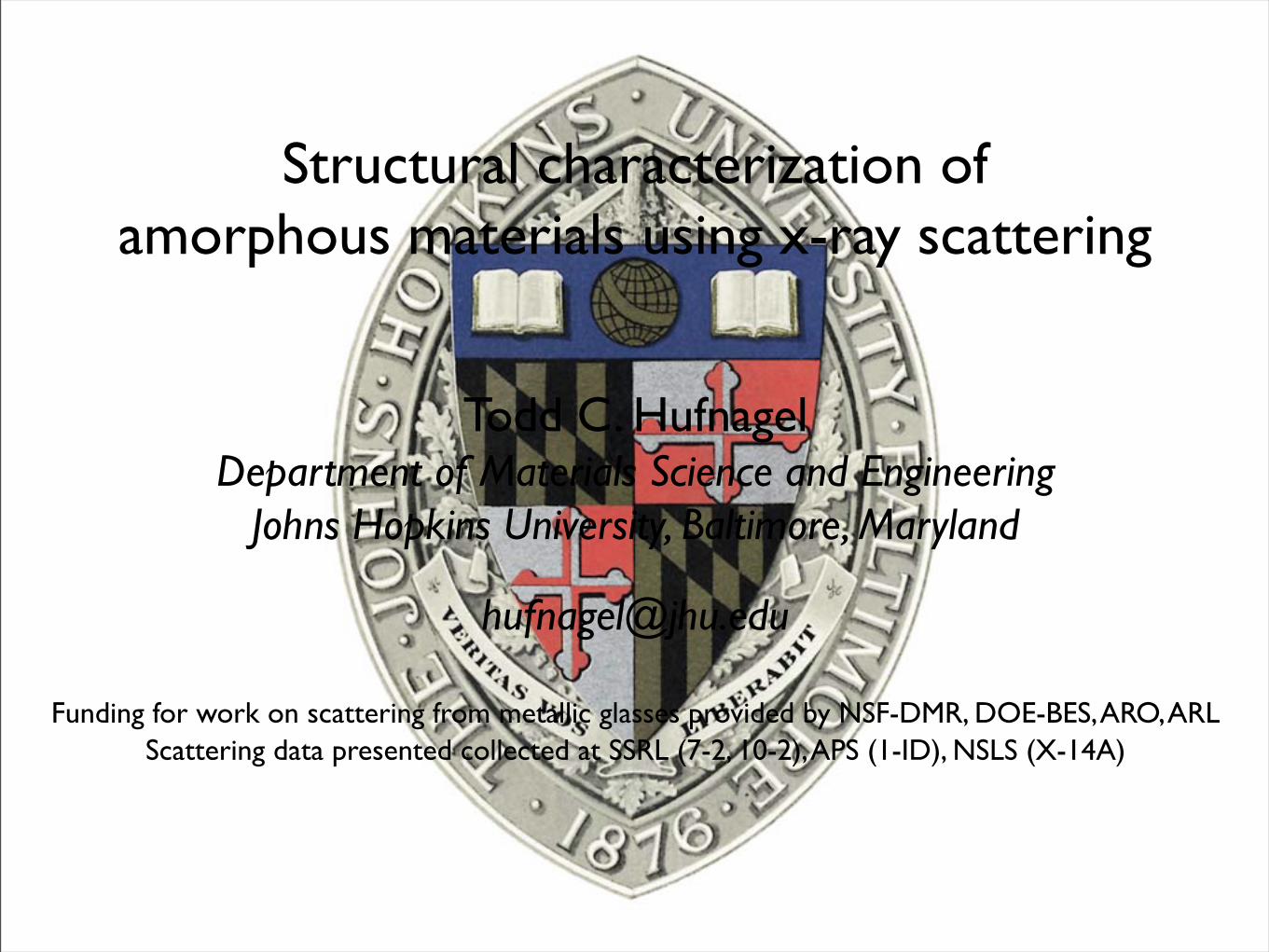
Outline
1.How is scattering from amorphous materials different from diffraction from crystalline materials?
2.A gentle introduction to the theory of scattering from amorphous materials, and the structural information you get.
3.The path to enlightenment: From raw data to real-space structure
4.Experimental techniques and considerations
5.Resonant scattering
6.Resources
T. C. Hufnagel, Johns Hopkins University
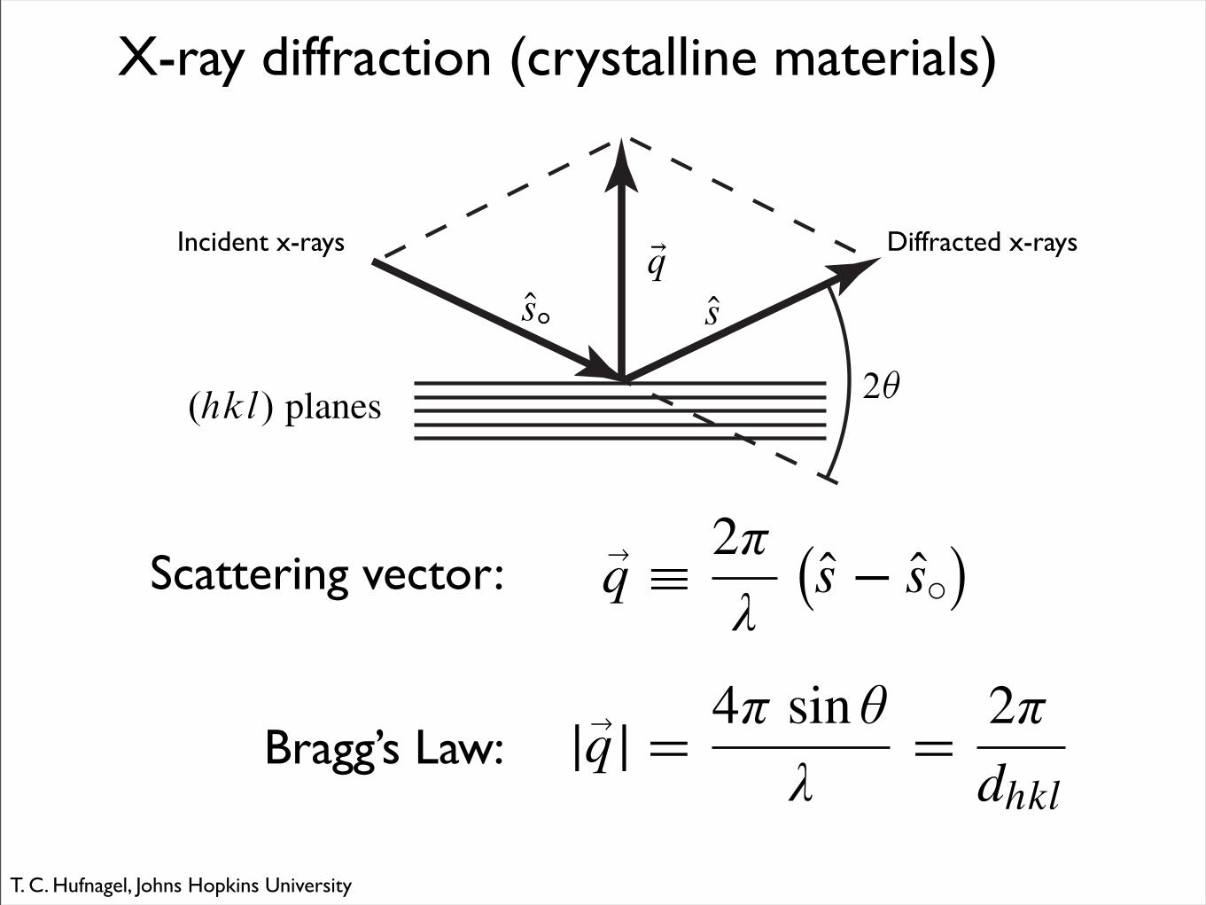
!q " 2!
"
!s # s$
"
|!q| = 4! sin "
#= 2!
dhkl
X-ray diffraction (crystalline materials)
.hkl/ planes 2!
EqOsOsı
Scattering vector:
Bragg’s Law:
Incident x-rays Diffracted x-rays
T. C. Hufnagel, Johns Hopkins University
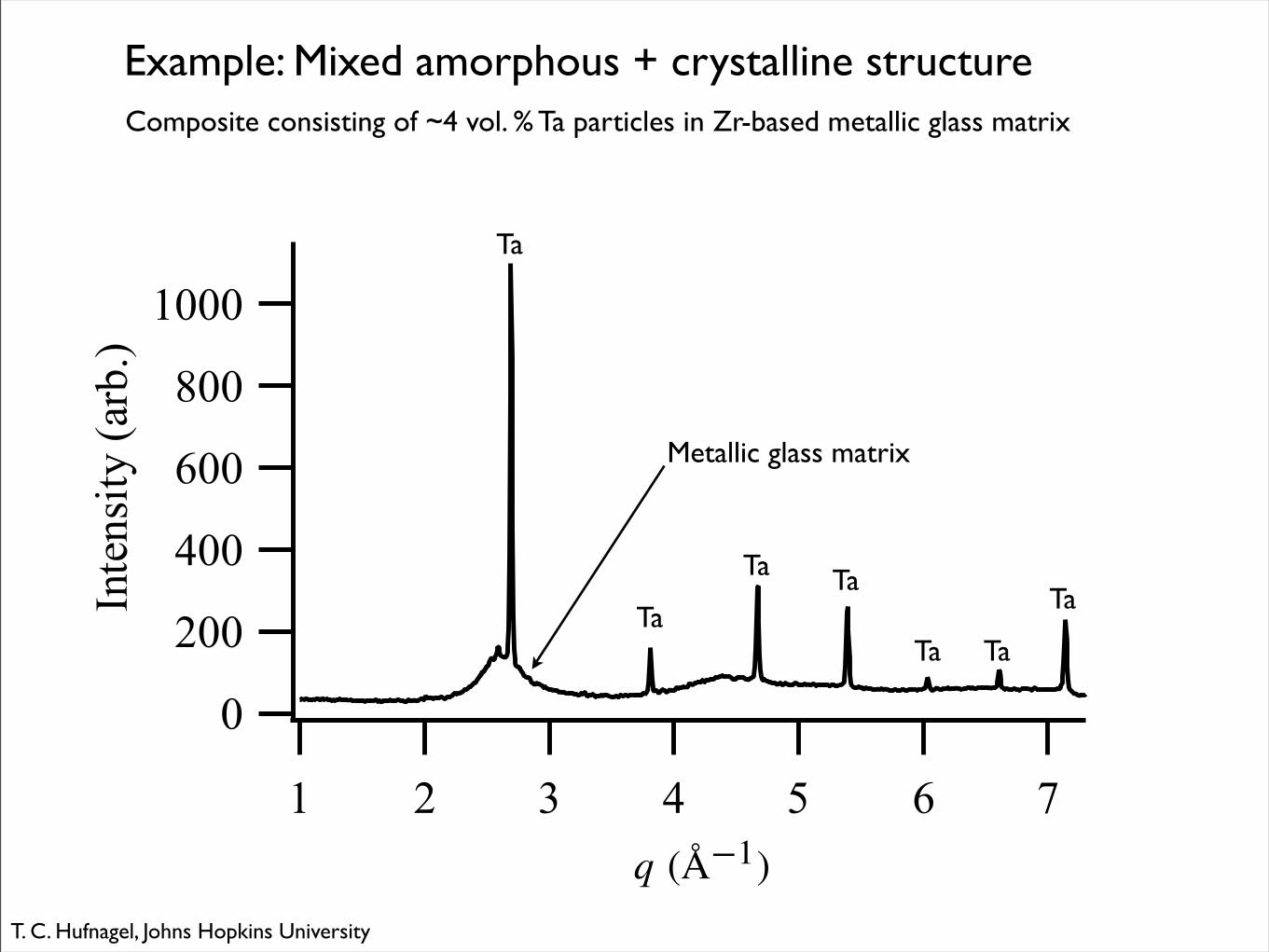
q (A!1)
Composite consisting of ~4 vol. % Ta particles in Zr-based metallic glass matrix
Example: Mixed amorphous + crystalline structure
Ta
Ta
Ta Ta
Ta Ta
Ta
Metallic glass matrix
T. C. Hufnagel, Johns Hopkins University

Crystalline AmorphousScattering is strong
(intense peaks)Scattering is weak
Scattering concentrated into a few sharp diffraction peaks
Scattering spread throughout reciprocal space (all values of q)
Data easilyinterpreted using simple equations
Detailed analysisrequired to obtain
real-space information
T. C. Hufnagel, Johns Hopkins University
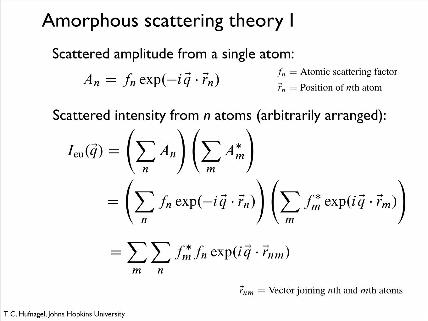
Amorphous scattering theory I
An D fn exp.!i Eq " Ern/
Scattered amplitude from a single atom:
Scattered intensity from n atoms (arbitrarily arranged):
D X
n
fn exp.!i Eq " Ern/
! X
m
f !m exp.i Eq " Erm/
!
DX
m
X
n
f !mfn exp.i Eq ! Ernm/
Ieu.Eq/ D X
n
An
! X
m
A!m
!
fn D Atomic scattering factor
Ern D Position of nth atom
Ernm D Vector joining nth and mth atoms
T. C. Hufnagel, Johns Hopkins University
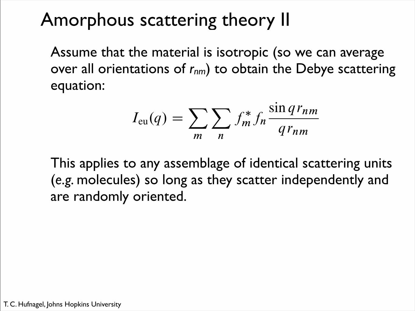
Amorphous scattering theory II
Assume that the material is isotropic (so we can averageover all orientations of rnm) to obtain the Debye scattering equation:
Ieu.q/ DX
m
X
n
f !mfn
sin qrnm
qrnm
This applies to any assemblage of identical scattering units(e.g. molecules) so long as they scatter independently andare randomly oriented.
T. C. Hufnagel, Johns Hopkins University
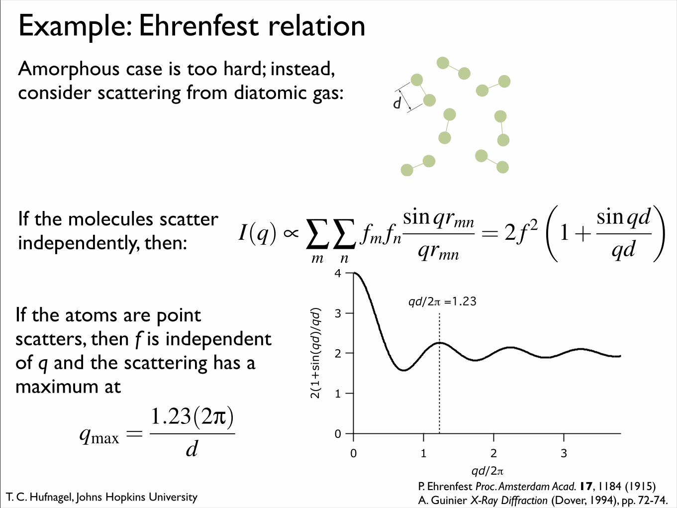
Example: Ehrenfest relation
P. Ehrenfest Proc. Amsterdam Acad. 17, 1184 (1915)A. Guinier X-Ray Diffraction (Dover, 1994), pp. 72-74.
Amorphous case is too hard; instead, consider scattering from diatomic gas:
d
If the molecules scatterindependently, then: I(q) ! "
m"n
fm fnsinqrmn
qrmn= 2 f 2
!1+
sinqdqd
"
If the atoms are point scatters, then f is independent of q and the scattering has a maximum at
qmax =1.23(2!)
d!
!
T. C. Hufnagel, Johns Hopkins University
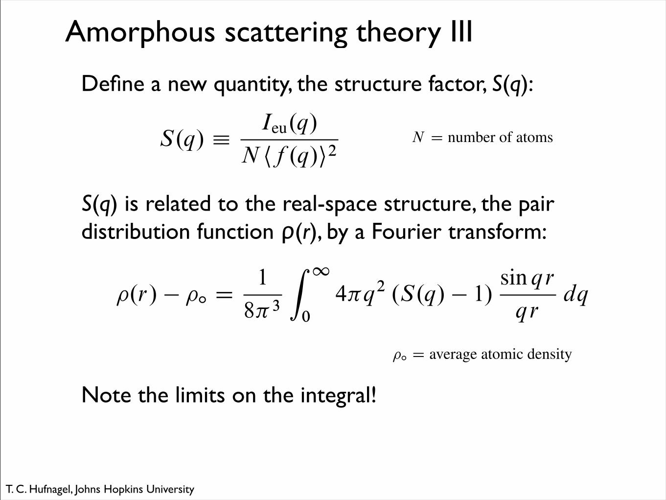
Amorphous scattering theory III
Define a new quantity, the structure factor, S(q):
S.q/ ! Ieu.q/
N hf .q/i2
S(q) is related to the real-space structure, the pair distribution function ρ(r), by a Fourier transform:
!.r/ ! !ı D 1
8"3
Z 1
0
4"q2 .S.q/ ! 1/sin qr
qrdq
Note the limits on the integral!
N D number of atoms
!ı D average atomic density
T. C. Hufnagel, Johns Hopkins University
S(q)
!(r
)(A
!3)
q (A!1) r (A)
(a) (b)
RD
F,4!
r2 "(r
)(A
!1)
r (A)
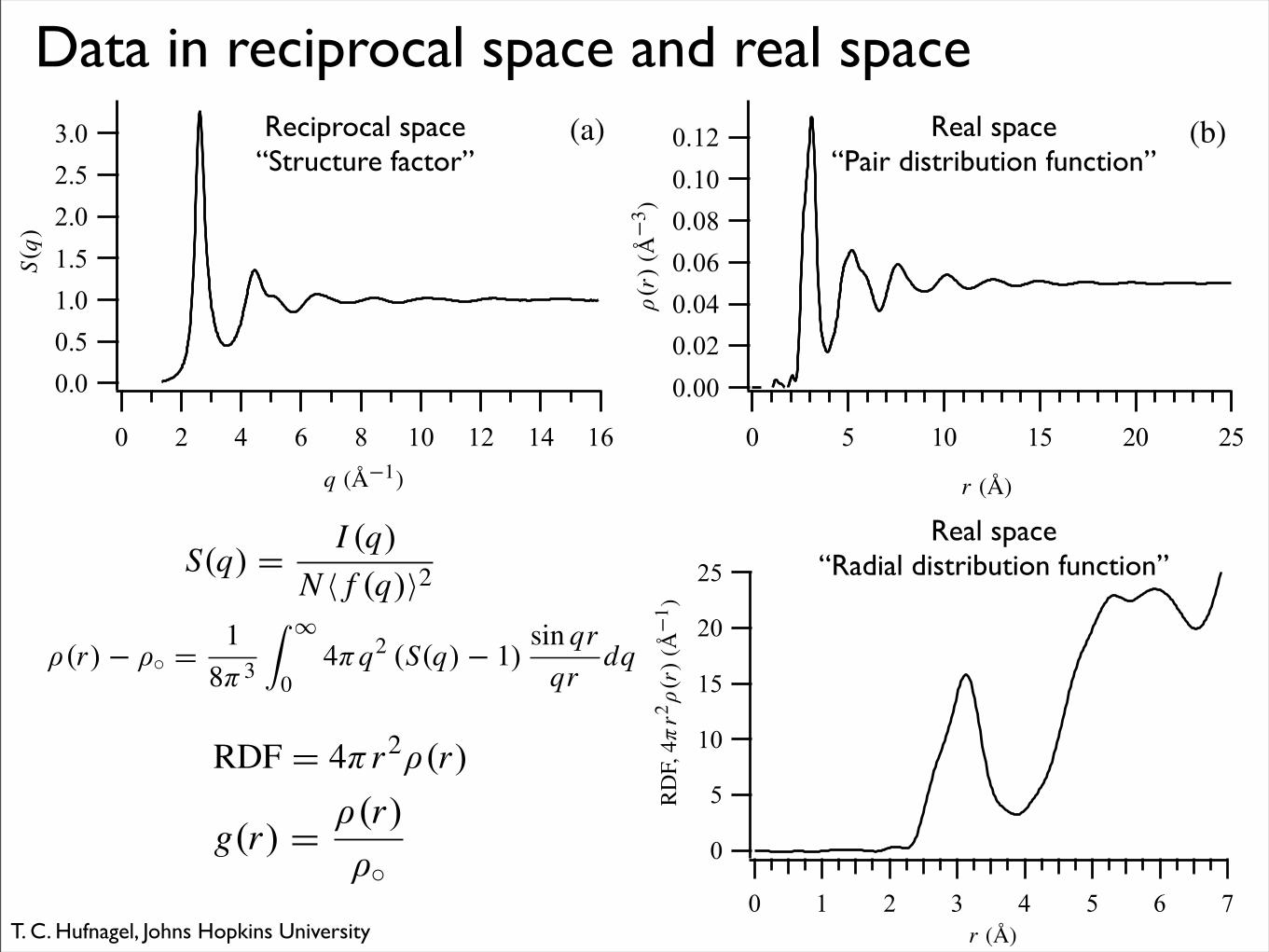
Data in reciprocal space and real spaceReciprocal space
“Structure factor”Real space
“Pair distribution function”
S(q) = I (q)
N ! f (q)"2
!(r) ! !" = 18"3
! #
04"q2 (S(q) ! 1)
sin qrqr
dq
Real space“Radial distribution function”
RDF = 4!r2"(r)
g(r) = !(r)
!!T. C. Hufnagel, Johns Hopkins University
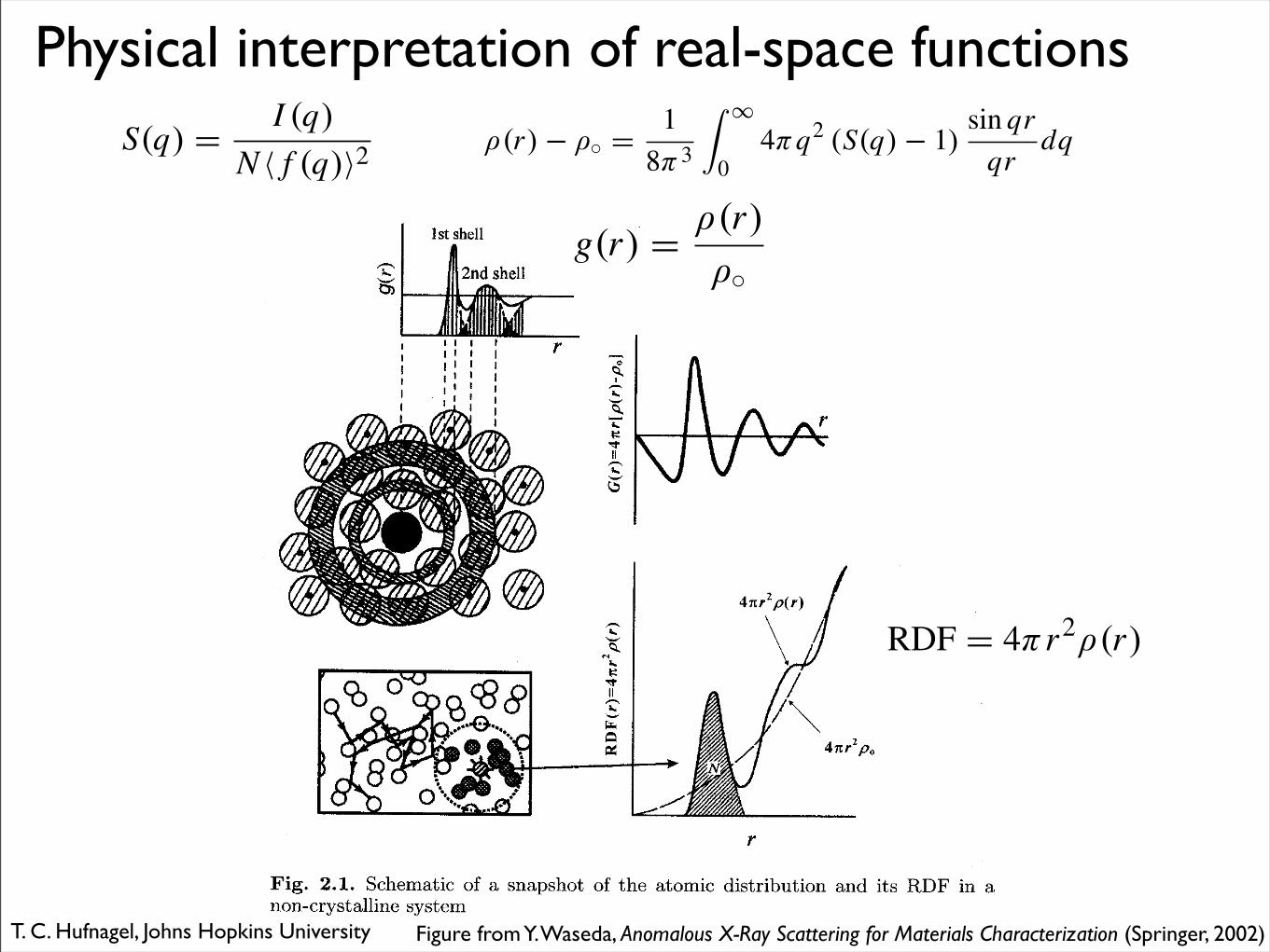
Physical interpretation of real-space functionsS(q) = I (q)
N ! f (q)"2 !(r) ! !" = 18"3
! #
04"q2 (S(q) ! 1)
sin qrqr
dq
RDF = 4!r2"(r)
g(r) = !(r)
!!
Figure from Y. Waseda, Anomalous X-Ray Scattering for Materials Characterization (Springer, 2002)T. C. Hufnagel, Johns Hopkins University
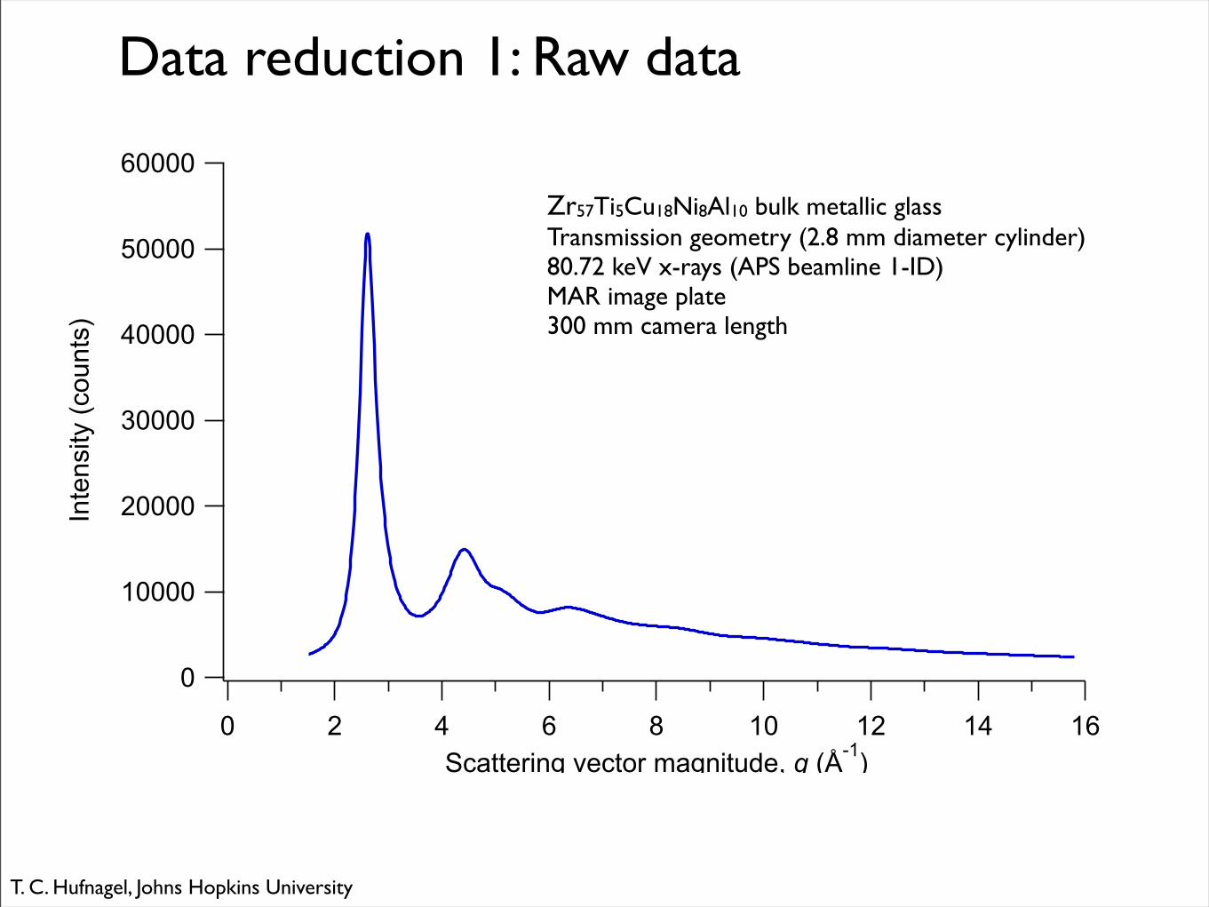
Data reduction 1: Raw data
Zr57Ti5Cu18Ni8Al10 bulk metallic glassTransmission geometry (2.8 mm diameter cylinder)80.72 keV x-rays (APS beamline 1-ID)MAR image plate300 mm camera length
60000
50000
40000
30000
20000
10000
0
Inte
nsi
ty (
counts
)
1614121086420
Scattering vector magnitude, q (Å-1
)
T. C. Hufnagel, Johns Hopkins University
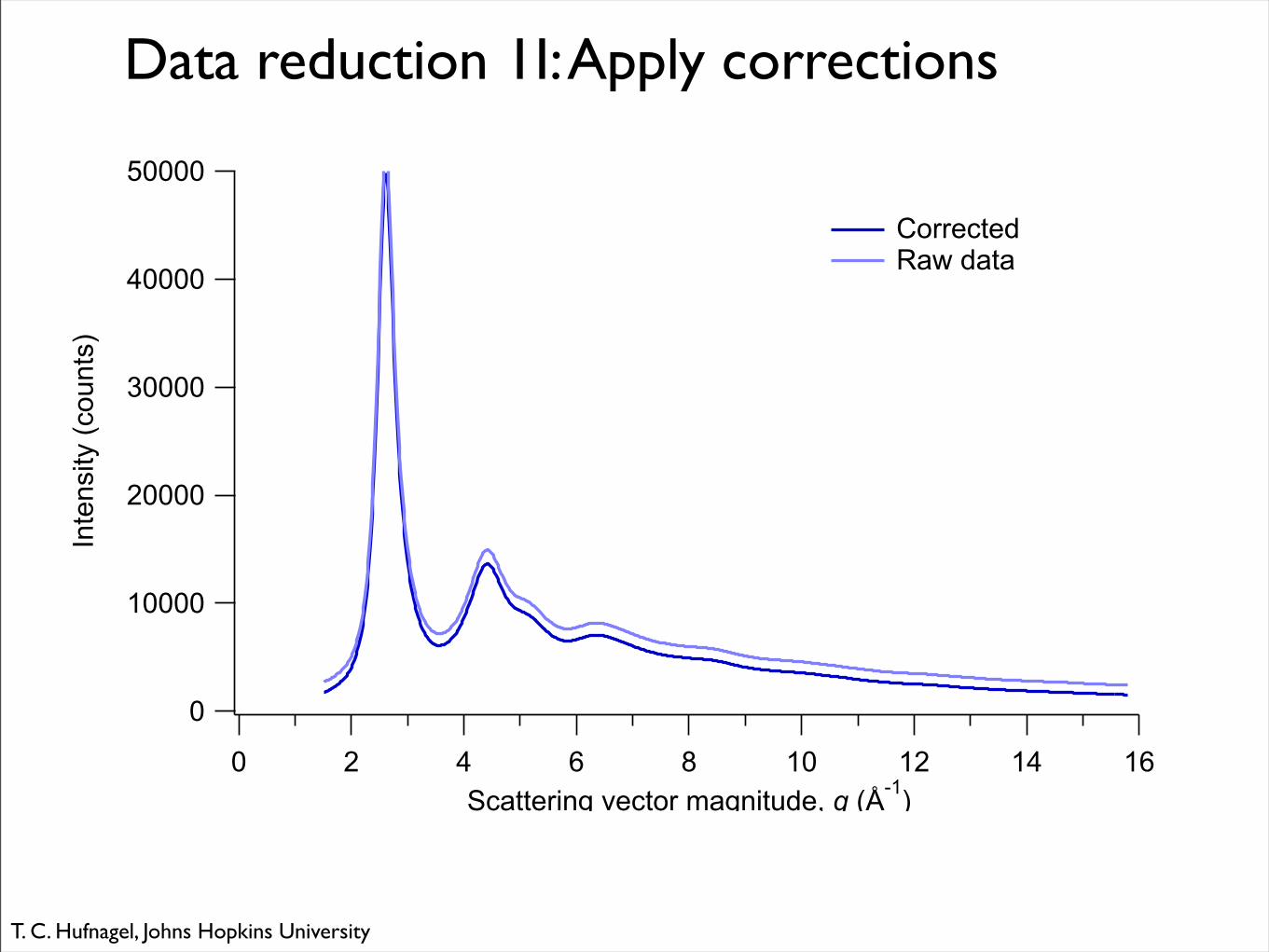
Data reduction 1I: Apply corrections
50000
40000
30000
20000
10000
0
Inte
nsi
ty (
counts
)
1614121086420
Scattering vector magnitude, q (Å-1
)
Corrected Raw data
T. C. Hufnagel, Johns Hopkins University
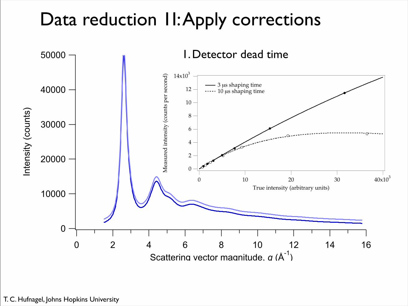
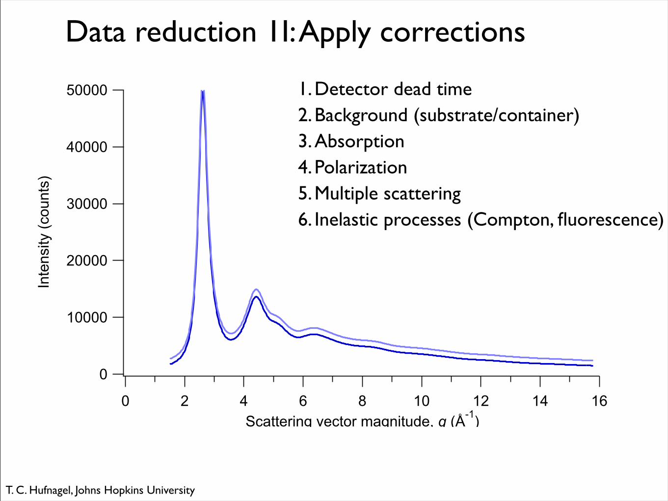
Data reduction 1I: Apply corrections
50000
40000
30000
20000
10000
0
Inte
nsi
ty (
cou
nts
)
1614121086420
Scattering vector magnitude, q (Å-1
)
1.Detector dead time
14x103
12
10
8
6
4
2
0Mea
sure
d in
tens
ity (c
ount
s pe
r se
cond
)
40x103 3020100True intensity (arbitrary units)
3 µs shaping time 10 µs shaping time
T. C. Hufnagel, Johns Hopkins University
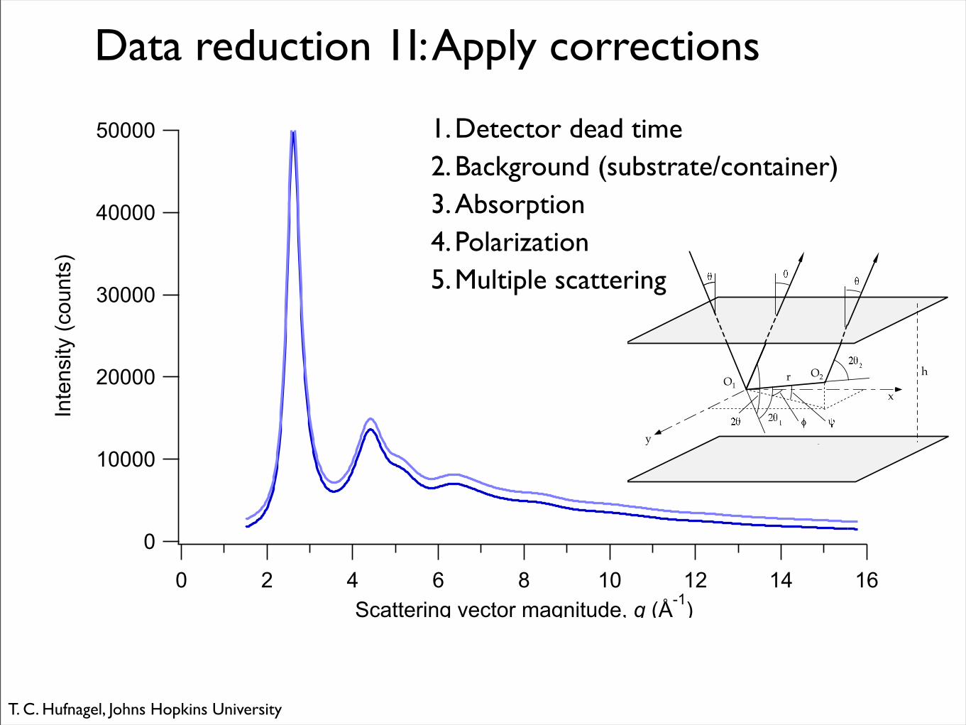
Data reduction 1I: Apply corrections
50000
40000
30000
20000
10000
0
Inte
nsi
ty (
cou
nts
)
1614121086420
Scattering vector magnitude, q (Å-1
)
1.Detector dead time2.Background (substrate/container)3.Absorption4.Polarization5.Multiple scattering
O1O2
y
x
hr
T. C. Hufnagel, Johns Hopkins University
Data reduction 1I: Apply corrections
50000
40000
30000
20000
10000
0
Inte
nsi
ty (
cou
nts
)
1614121086420
Scattering vector magnitude, q (Å-1
)
1.Detector dead time2.Background (substrate/container)3.Absorption4.Polarization5.Multiple scattering6.Inelastic processes (Compton, fluorescence)
T. C. Hufnagel, Johns Hopkins University
2500
2000
1500
1000
500
0
Inte
nsi
ty (
ele
ctro
n u
nits
)
1614121086420
Scattering vector magnitude, q (Å-1
)
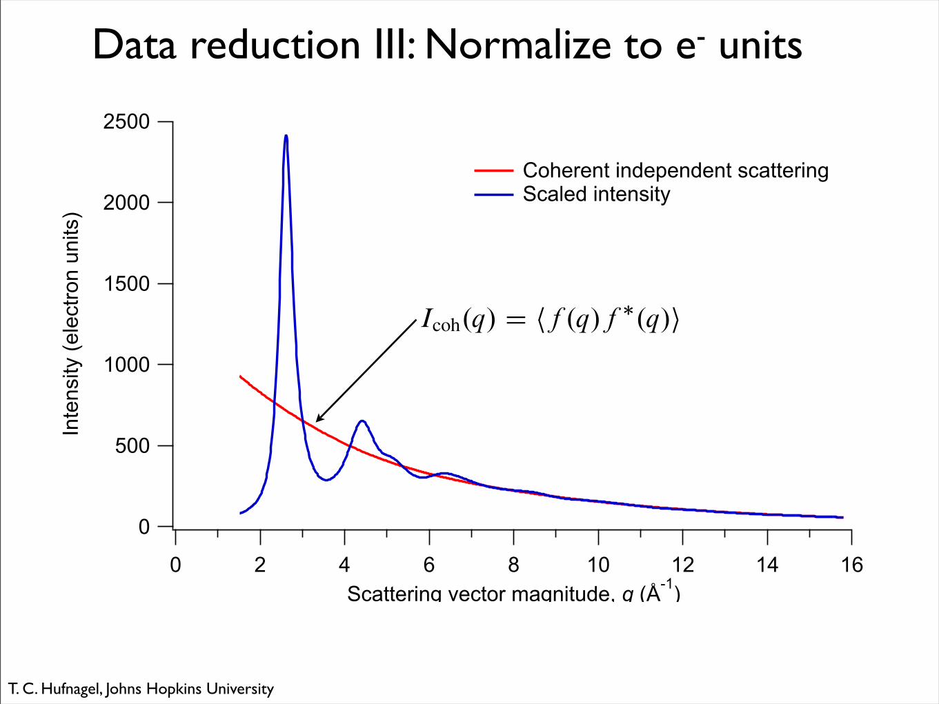
Coherent independent scattering Scaled intensity
Data reduction III: Normalize to e- units
Icoh.q/ D hf .q/f !.q/i
T. C. Hufnagel, Johns Hopkins University
4
3
2
1
0
S(q
)
1614121086420
Scattering vector magnitude, q (Å-1
)
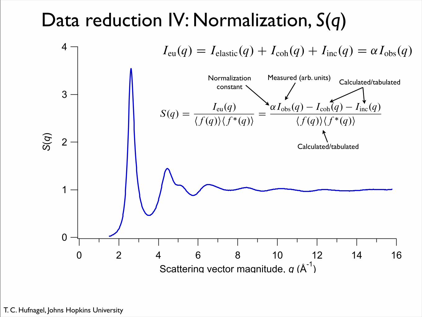
Data reduction IV: Normalization, S(q)Ieu.q/ D Ielastic.q/ C Icoh.q/ C Iinc.q/ D ˛Iobs.q/
S.q/ D Ieu.q/
hf .q/ihf !.q/i D ˛Iobs.q/ ! Icoh.q/ ! Iinc.q/
hf .q/ihf !.q/i
Measured (arb. units)Calculated/tabulated
Calculated/tabulated
Normalizationconstant
T. C. Hufnagel, Johns Hopkins University
Data reduction IV: Normalization, S(q)4
3
2
1
0
S(q
)
1614121086420
Scattering vector magnitude, q (Å-1
)
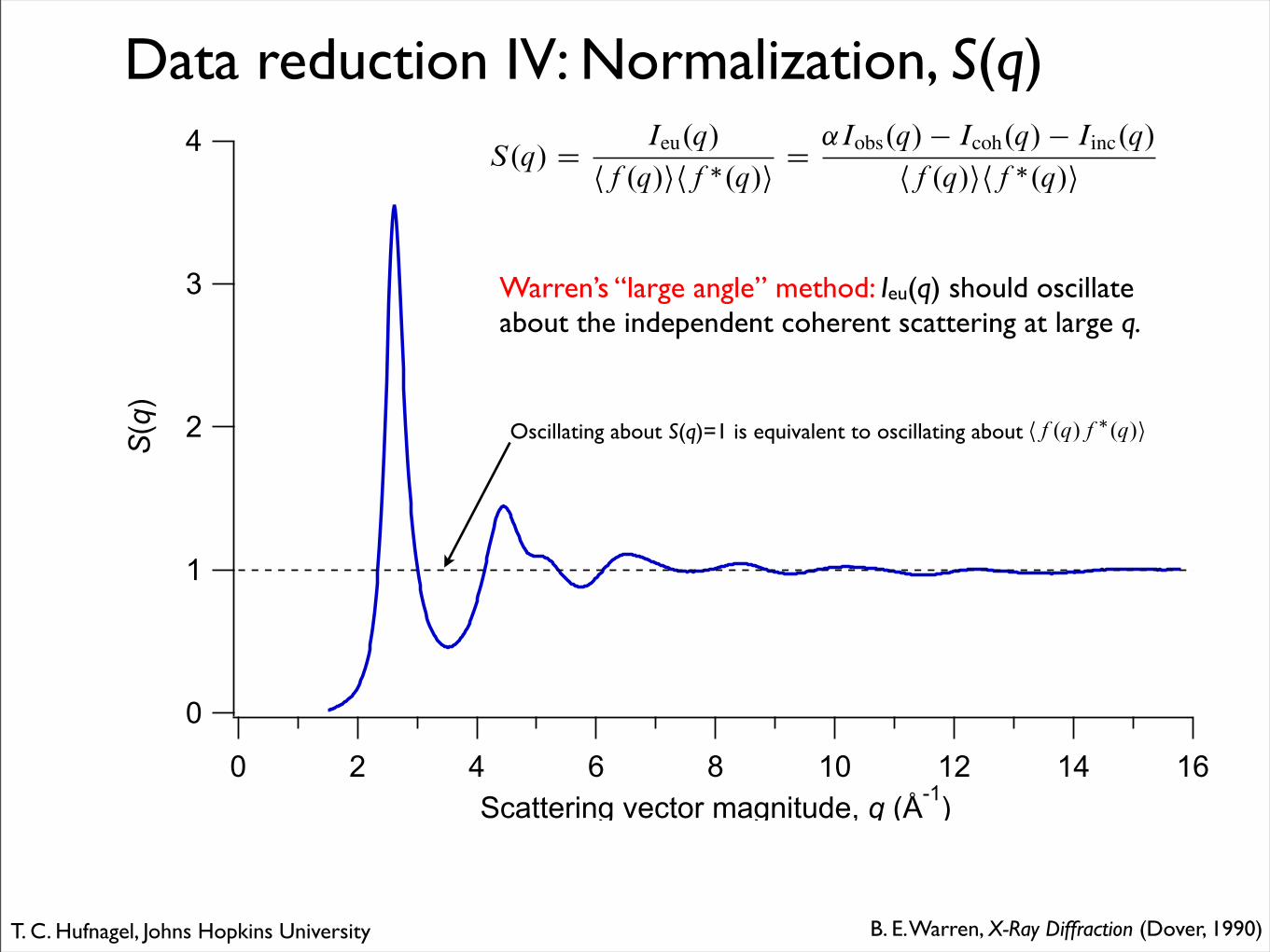
Oscillating about S(q)=1 is equivalent to oscillating about hf .q/f !.q/i
S.q/ D Ieu.q/
hf .q/ihf !.q/i D ˛Iobs.q/ ! Icoh.q/ ! Iinc.q/
hf .q/ihf !.q/i
Warren’s “large angle” method: Ieu(q) should oscillate about the independent coherent scattering at large q.
B. E. Warren, X-Ray Diffraction (Dover, 1990)T. C. Hufnagel, Johns Hopkins University

Data reduction IV: Normalization, S(q)4
3
2
1
0
S(q
)
1614121086420
Scattering vector magnitude, q (Å-1
)
S.q/ D Ieu.q/
hf .q/ihf !.q/i D ˛Iobs.q/ ! Icoh.q/ ! Iinc.q/
hf .q/ihf !.q/i
Norman/Krogh-Moe (“integral”) method: Makes use of the fact that ρ(r)→ at low r to obtain:
˛ DR 1
0 q2Icoh.q/ dq ! 2!2"ıhf .q/ihf !.q/iR 1
0 q2Iobs.q/ dq:
N. Norman, Acta Crystallogr. 10, 370 (1957)J. Krogh-Moe, Acta Crystallogr. 9, 951 (1956)T. C. Hufnagel, Johns Hopkins University

Data reduction V: Real-space functions
0.12
0.10
0.08
0.06
0.04
0.02
0.00
Pa
ir d
istr
ibu
tion
fu
nct
ion
, !
(r)
(Å-3
)
20151050
Distance from central atom, r (Å)
!(r) ! !" = 18"3
! #
04"q2 (S(q) ! 1)
sin qrqr
dq
Upper limit set by experiment
Positions of peaks→Coordination shell distances
T. C. Hufnagel, Johns Hopkins University

Data reduction V: Real-space functions
50
40
30
20
10
0
Ra
dia
l dis
trib
utio
n f
un
ctio
n,
4!r2"
(r)(
ato
ms
Å-1
)
1086420
Distance from central atom, r (Å)
RDF = 4!r2"(r)
Area under peak = coordination number
4!r2"ıInspect the low r region...should be zero!(Large oscillations are a sign of trouble withnormalization, corrections, and/or damping.)
T. C. Hufnagel, Johns Hopkins University
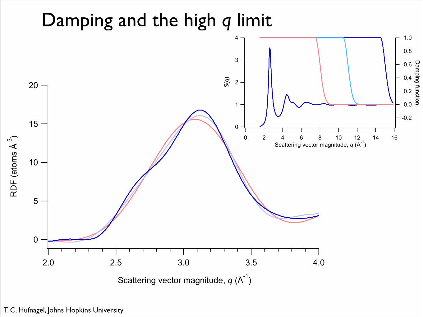
Damping and the high q limit4
3
2
1
0
S(q
)
1614121086420Scattering vector magnitude, q (Å
-1)
1.0
0.8
0.6
0.4
0.2
0.0
-0.2
Dam
pin
g fu
nctio
n
20
15
10
5
0
RD
F (
ato
ms
Å-3
)
4.03.53.02.52.0
Scattering vector magnitude, q (Å-1
)
T. C. Hufnagel, Johns Hopkins University
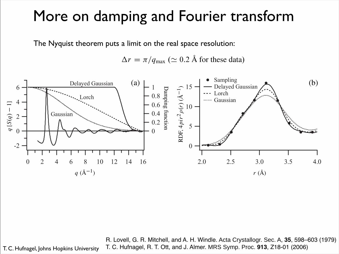
More on damping and Fourier transform
q (A!1)
q[S
(q)!
1 ]
RD
F,4p
ir2 !
(r)
(A!1
)Dam
pingfunction
r (A)
(a) (b)
R. Lovell, G. R. Mitchell, and A. H. Windle. Acta Crystallogr. Sec. A, 35, 598–603 (1979)T. C. Hufnagel, R. T. Ott, and J. Almer. MRS Symp. Proc. 913, Z18-01 (2006)
The Nyquist theorem puts a limit on the real space resolution:
!r D "=qmax .' 0:2 A for these data/
T. C. Hufnagel, Johns Hopkins University
0.0001
0.001
0.01
0.1
1
10
r(g(r
)-1)
252015105
r (Å)
0% Ta!=3.8±0.2 Å
4% Ta!=5.3±0.2 Å
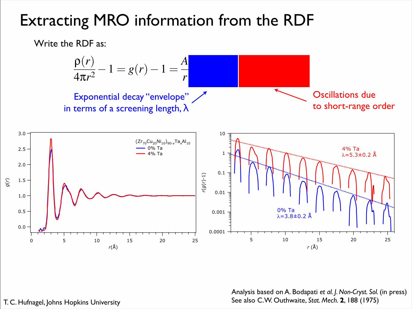
Extracting MRO information from the RDF
3.0
2.5
2.0
1.5
1.0
0.5
0.0
g(r
)
2520151050r(Å)
(Zr70Cu20Ni10)90-xTaxAl10
0% Ta 4% Ta
Exponential decay “envelope”in terms of a screening length, λ
Write the RDF as:
Oscillations dueto short-range order
ρ(r)4πr2−1 = g(r)−1 =
Ar
exp(−r
λ
)sin
(2πrD
+φ)
Analysis based on A. Bodapati et al. J. Non-Cryst. Sol. (in press)See also C.W. Outhwaite, Stat. Mech. 2, 188 (1975) T. C. Hufnagel, Johns Hopkins University
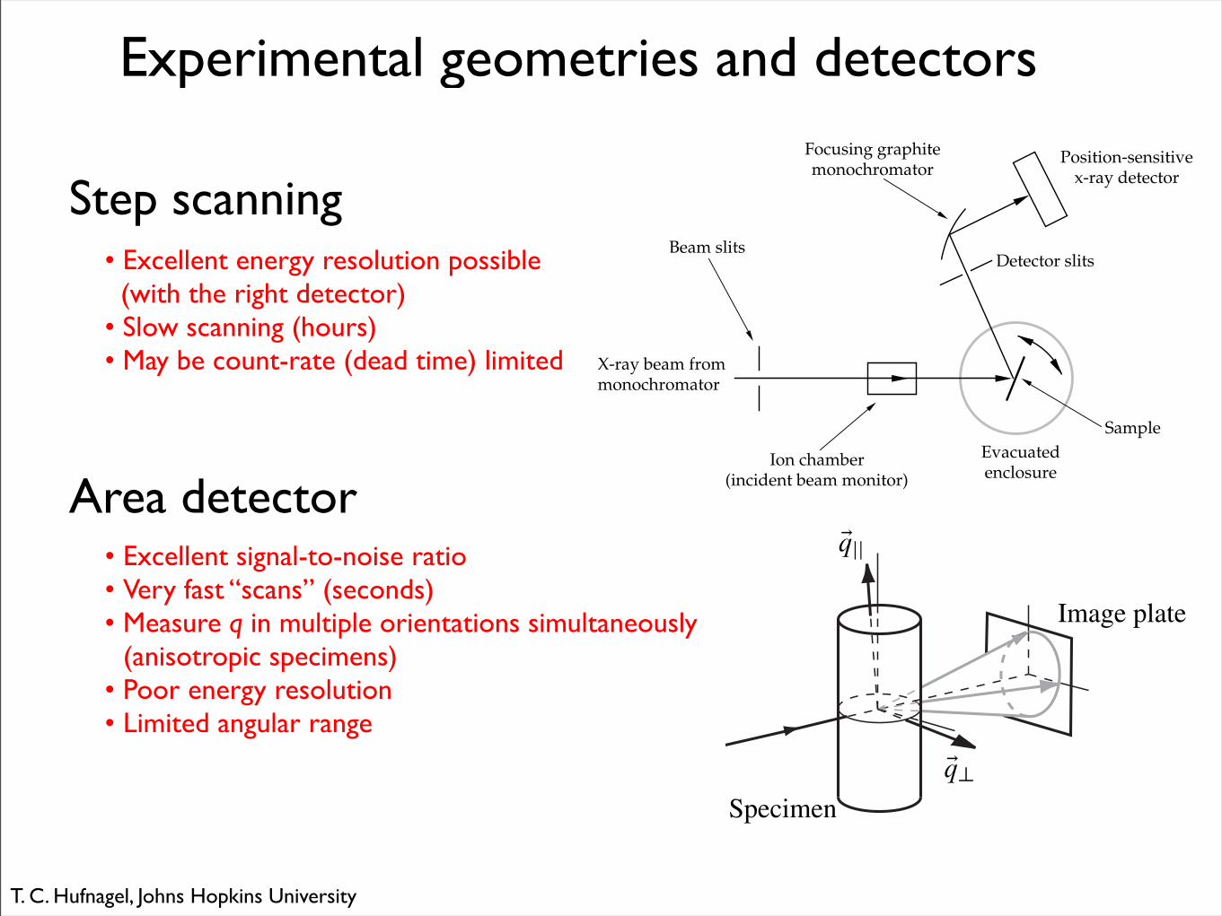
Experimental geometries and detectors
Evacuatedenclosure
Sample
X-ray beam frommonochromator
Beam slits
Ion chamber(incident beam monitor)
Detector slits
Focusing graphitemonochromator
Position-sensitivex-ray detector
Step scanning
Eq?
Eqjj
Image plate
Specimen
• Excellent energy resolution possible (with the right detector) • Slow scanning (hours) • May be count-rate (dead time) limited
• Excellent signal-to-noise ratio • Very fast “scans” (seconds) • Measure q in multiple orientations simultaneously (anisotropic specimens) • Poor energy resolution • Limited angular range
Area detector
T. C. Hufnagel, Johns Hopkins University

• Need to measure I(q) to the largest q possible:
• The elastic, single-scattering intensity I(q) must be separated from all other sources of intensity. (This usually involves both experimental design and data analysis.)
• High signal-to-noise is essential at all values of q, especially at high q:
Data collection considerations
qmax D 4!
"D 4!E
hcqmax.A!1
/ ! E.keV/
!(r) ! !" = 18"3
! #
04"q2 (S(q) ! 1)
sin qrqr
dq
T. C. Hufnagel, Johns Hopkins University
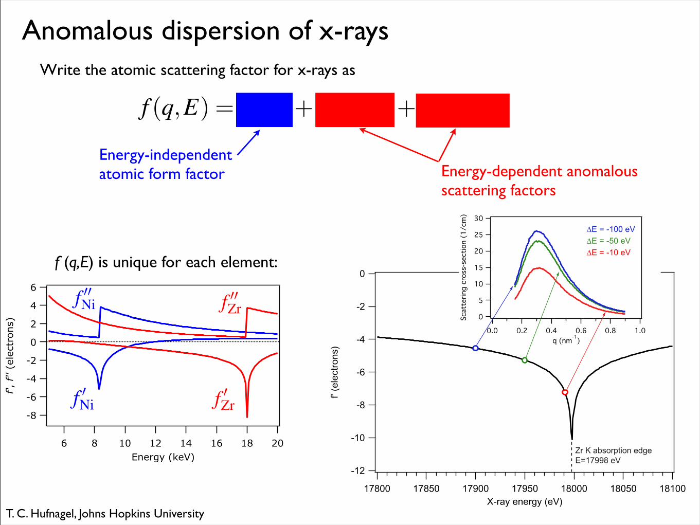
Anomalous dispersion of x-raysWrite the atomic scattering factor for x-rays as
f (q,E) = f!(q)+ f "(q,E)+ i f ""(q,E)
Energy-dependent anomalous scattering factors
Energy-independentatomic form factor
-8
-6
-4
-2
0
2
4
6
f', f'' (e
lect
rons)
20181614121086Energy (keV)
-12
-10
-8
-6
-4
-2
0
f' (e
lect
rons
)
18100180501800017950179001785017800X-ray energy (eV)
30
25
20
15
10
5
0Scat
terin
g cr
oss-
sect
ion
(1/c
m)
1.00.80.60.40.20.0q (nm-1)
!E = -100 eV
!E = -50 eV
!E = -10 eV
Zr K absorption edgeE=17998 eV
f (q,E) is unique for each element:
f !Zr
f !!Zr
f !!Ni
f !Ni
T. C. Hufnagel, Johns Hopkins University
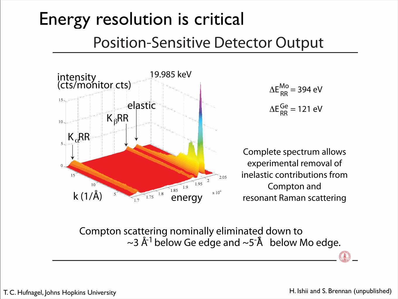
Energy resolution is criticalPosition-Sensitive Detector Output
energyk (1/Å)
elastic
K RR!
K RR"
intensity(cts/monitor cts)
19.985 keV
Complete spectrum allowsexperimental removal of
inelastic contributions fromCompton and
resonant Raman scattering
Compton scattering nominally eliminated down to ~3 Å below Ge edge and ~5 Å below Mo edge.-1 -1
#E = 394 eV
#E = 121 eV
Mo
Ge
RR
RR
H. Ishii and S. Brennan (unpublished)T. C. Hufnagel, Johns Hopkins University
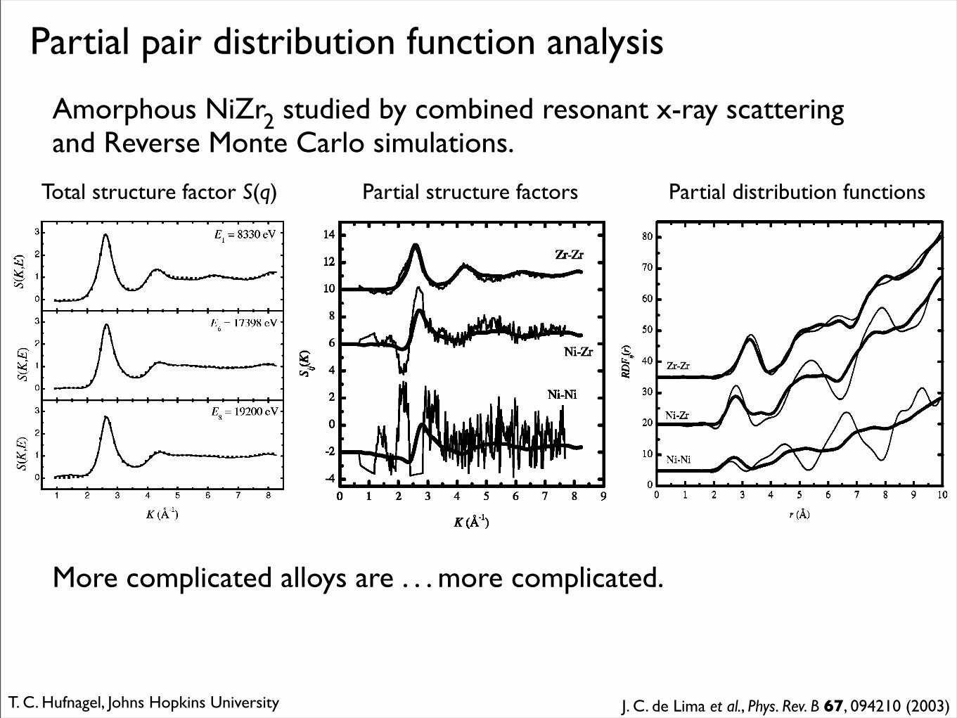
Partial pair distribution function analysis
Amorphous NiZr studied by combined resonant x-ray scattering and Reverse Monte Carlo simulations.
2
Total structure factor S(q) Partial structure factors Partial distribution functions
J. C. de Lima et al., Phys. Rev. B 67, 094210 (2003)
More complicated alloys are . . . more complicated.
T. C. Hufnagel, Johns Hopkins University
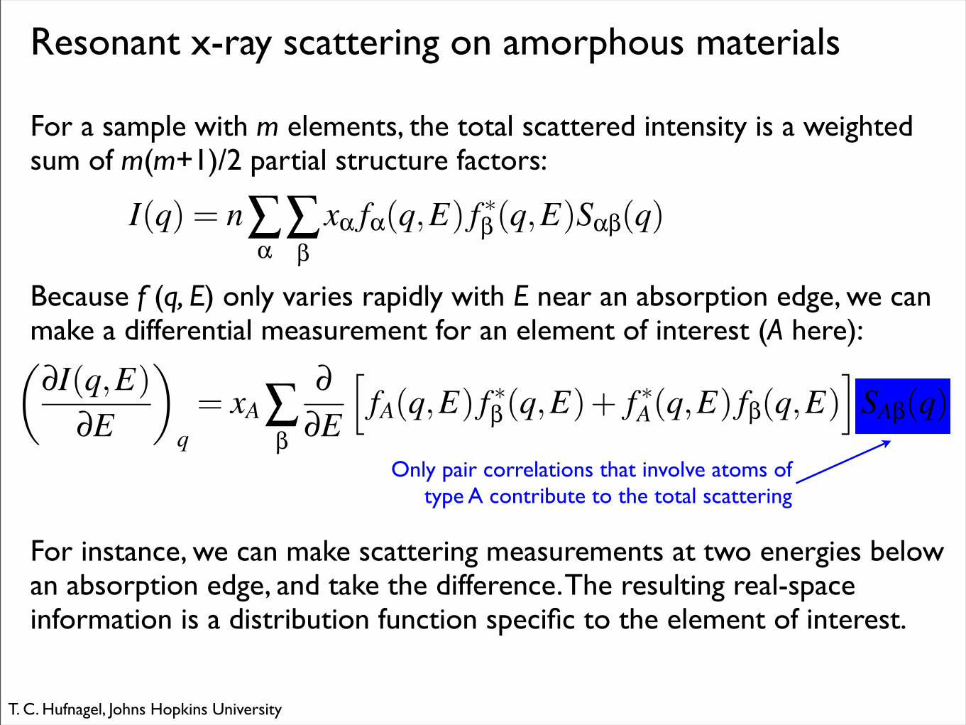
Resonant x-ray scattering on amorphous materials
For a sample with m elements, the total scattered intensity is a weighted sum of m(m+1)/2 partial structure factors:
Only pair correlations that involve atoms of type A contribute to the total scattering
I(q) = n!"
!#
x" f"(q,E) f !#(q,E)S"#(q)
Because f (q, E) only varies rapidly with E near an absorption edge, we can make a differential measurement for an element of interest (A here):
For instance, we can make scattering measurements at two energies below an absorption edge, and take the difference. The resulting real-space information is a distribution function specific to the element of interest.
!!I(q,E)
!E
"
q= xA"
#
!!E
#fA(q,E) f !#(q,E)+ f !A(q,E) f#(q,E)
$SA#(q)
T. C. Hufnagel, Johns Hopkins University
30
25
20
15
10
5
0
RD
F (a
tom
s/Å)
876543210r (Å)
(Zr70Cu20Ni10)90-xTaxAl10
0% Ta 4% Ta
30
25
20
15
10
5
0
Cu D
DF
(ato
ms/
Å)
876543210r (Å)
(Zr70Cu20Ni10)90-xTaxAl10
0% Ta 4% Ta
30
25
20
15
10
5
0
RD
F (a
tom
s/Å)
876543210r (Å)
(Zr70Cu20Ni10)90-xTaxAl10
0% Ta 4% Ta
30
25
20
15
10
5
0
Ta
DD
F (a
tom
s/Å)
876543210r (Å)
(Zr70Cu20Ni10)90-xTaxAl10
4% Ta
30
25
20
15
10
5
0
RD
F (a
tom
s/Å)
876543210r (Å)
(Zr70Cu20Ni10)90-xTaxAl10
0%Ta 4%Ta
30
25
20
15
10
5
0
Zr
DD
F (a
tom
s/Å)
876543210r (Å)
(Zr70Cu20Ni10)90-xTaxAl10
0% Ta 4% Ta
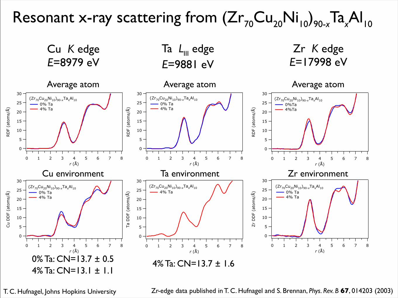
Resonant x-ray scattering from (Zr70Cu20Ni10)90-xTaxAl10
Cu K edgeE=8979 eV
Ta LIII edgeE=9881 eV
Zr K edgeE=17998 eV
Average atom
Cu environment
Average atom
Ta environment
Average atom
Zr environment
Zr-edge data published in T. C. Hufnagel and S. Brennan, Phys. Rev. B 67, 014203 (2003)
0% Ta: CN=13.7 ± 0.54% Ta: CN=13.1 ± 1.1
4% Ta: CN=13.7 ± 1.6
T. C. Hufnagel, Johns Hopkins University
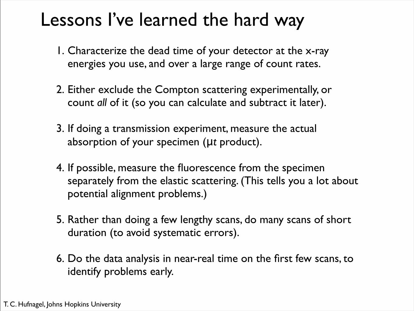
Lessons I’ve learned the hard way
1.Characterize the dead time of your detector at the x-ray energies you use, and over a large range of count rates.
2.Either exclude the Compton scattering experimentally, or count all of it (so you can calculate and subtract it later).
3. If doing a transmission experiment, measure the actual absorption of your specimen (μt product).
4.If possible, measure the fluorescence from the specimen separately from the elastic scattering. (This tells you a lot about potential alignment problems.)
5.Rather than doing a few lengthy scans, do many scans of short duration (to avoid systematic errors).
6.Do the data analysis in near-real time on the first few scans, to identify problems early.
T. C. Hufnagel, Johns Hopkins University
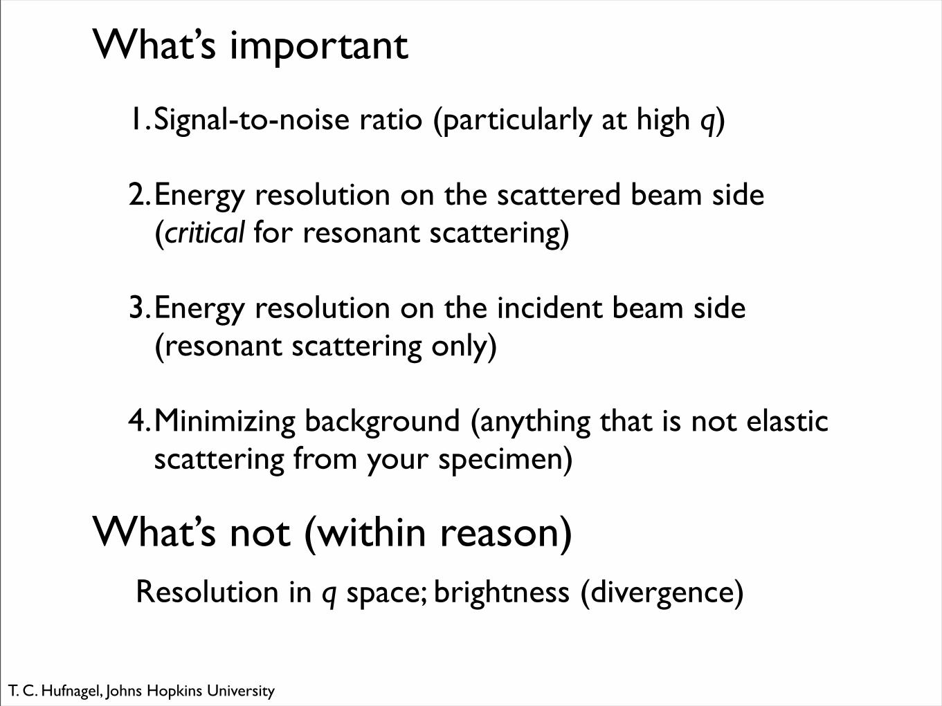
What’s important
1.Signal-to-noise ratio (particularly at high q)
2.Energy resolution on the scattered beam side (critical for resonant scattering)
3.Energy resolution on the incident beam side (resonant scattering only)
4.Minimizing background (anything that is not elastic scattering from your specimen)
What’s not (within reason)Resolution in q space; brightness (divergence)
T. C. Hufnagel, Johns Hopkins University

“X-ray amorphous”
100
80
60
40
20
0
Inte
nsity
(arb
. uni
ts)
5.04.03.02.0Scattering vector magnitude (Å-1)
Laboratory sourceCu Kα radiation (λ=1.54 Å)
100
80
60
40
20
0
Inte
nsity
(arb
. uni
ts)
5.04.03.02.0Scattering vector magnitude (Å-1)
Synchrotron sourceE=17898 eV (λ=0.693 Å)
Is it amorphous? • First peak symmetric • Second peak at ~1.6-1.8 qmax (for a metallic glass) • No other scattering features present • Combine with other techniques (TEM, DSC)
Fundamental problem: All you get (from scattering) is the RDF,which is only sensitive to pair correlations.
T. C. Hufnagel, Johns Hopkins University

0.012
0.010
0.008
0.006
0.004
0.002
0.000
Nor
mal
ized
var
ianc
e
543210Scattering vector magnitude, k (nm-1)
Zr59Ta5Cu18Ni8Al10 Zr57Ti5Cu20Ni8Al10
J. Li, X. Gu, and T. C. Hufnagel. Microscopy and Microanalysis 9, 509 (2003)
T. C. Hufnagel, Nature Mat. 3, 666 (2004)(figure adapted from P. M. Voyles)
Beyond the RDF: Fluctuation microscopy
The variance contains informationabout higher order (3- and 4-body)correlations
T. C. Hufnagel, Johns Hopkins University
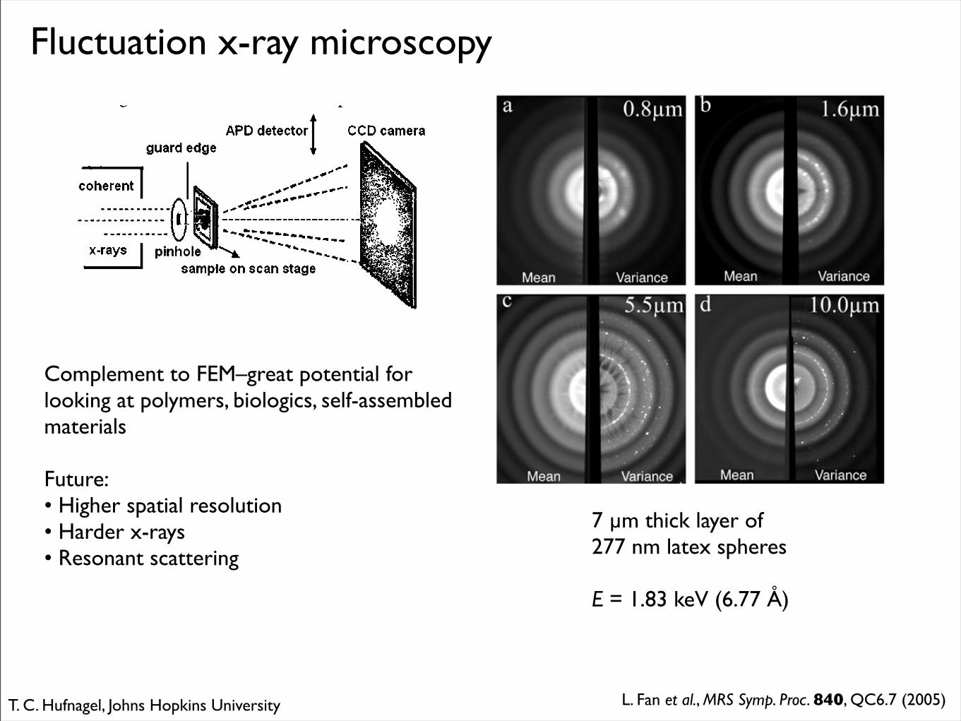
L. Fan et al., MRS Symp. Proc. 840, QC6.7 (2005)
Fluctuation x-ray microscopy
7 µm thick layer of277 nm latex spheres
E = 1.83 keV (6.77 Å)
Complement to FEM–great potential for looking at polymers, biologics, self-assembled materials
Future:• Higher spatial resolution• Harder x-rays• Resonant scattering
T. C. Hufnagel, Johns Hopkins University
References and resources• Books
- B. E. Warren, X-Ray Diffraction (Dover, 1990)
- T. Egami and S. Billinge, Underneath the Bragg Peaks: Structural Analysis of Complex Materials (Pergamon, 2003)
• Dissertations/SSRL reports from the Bienenstockgroup (Fuoss, Kortright, Ludwig,Wilson,Ishii...)
• Software
- Matlab routines (http://ssrl.slac.stanford.edu/~bren/files/amorphous/)
- Billinge group software (http://www.pa.msu.edu/ftp/pub/billinge/)
T. C. Hufnagel, Johns Hopkins University