Embed Size (px)
Citation preview

Universita degli Studi di Cagliari
Facolta di Ingegneria
Dipartimento di Ingegneria Elettrica ed Elettronica
STRUCTURAL AND
GRAPH-BASED METHODS FOR
AUTOMATIC FINGERPRINT
CLASSIFICATION
PhD Thesis of: Alessandra Serrau
Supervisor: Prof. Fabio Roli
Dottorato di Ricerca in Ingegneria Elettronica e Informatica
XVIII CICLO

Contents
Preface vii
1 Introduction to Biometrics 1
1.1 Biometrics and properties . . . . . . . . . . . . . . . . . . . . 2
1.2 Main biometrics . . . . . . . . . . . . . . . . . . . . . . . . . . 3
1.3 Comparison between biometrics . . . . . . . . . . . . . . . . . 8
1.4 Biometric system structure . . . . . . . . . . . . . . . . . . . . 9
1.5 Requirements of a biometric system . . . . . . . . . . . . . . . 13
1.6 Biometric system evaluation . . . . . . . . . . . . . . . . . . . 14
1.7 Fingerprint biometric . . . . . . . . . . . . . . . . . . . . . . . 18
1.7.1 History of fingerprint recognition . . . . . . . . . . . . 18
1.7.2 Structure of fingerprints . . . . . . . . . . . . . . . . . 20
1.7.3 The Automatic Fingerprint Identification System . . . 24
2 Fingerprint Classification: State of Art 27
2.1 Statistical methods . . . . . . . . . . . . . . . . . . . . . . . . 30
2.2 Structural and graph-based methods . . . . . . . . . . . . . . 32
2.3 Multiple classifiers system to fingerprint classification . . . . . 35
i

3 Graph-Based Approach 37
3.1 Introduction . . . . . . . . . . . . . . . . . . . . . . . . . . . . 37
3.2 An appropriate data representation . . . . . . . . . . . . . . . 40
3.3 The pre-processor module . . . . . . . . . . . . . . . . . . . . 42
3.4 A structural-connesionist approach . . . . . . . . . . . . . . . 43
3.4.1 The DPAG generator module . . . . . . . . . . . . . . 45
3.4.2 Recursive neural networks for fingerprint classfication . 51
3.5 The structural K-nn approach . . . . . . . . . . . . . . . . . . 54
4 Ensembles and Combinations 60
4.1 Fusion of structural and statistical fingerprint classifiers . . . . 61
4.2 Ensembles of graph matchers . . . . . . . . . . . . . . . . . . 63
4.2.1 Ensembles of statistical vs. structural classifiers . . . . 66
4.2.2 Bagging of structural classifiers . . . . . . . . . . . . . 68
4.2.3 Ensembles of structural K-nn . . . . . . . . . . . . . . 68
5 Experimental Investigation 71
5.1 The data set . . . . . . . . . . . . . . . . . . . . . . . . . . . . 71
5.2 Combination of diverse structural classifiers . . . . . . . . . . 73
5.2.1 Comparison of structural classifiers performance . . . 73
5.2.2 Decision-level fusion of structural classifiers . . . . . . 75
5.3 Diverse combinations . . . . . . . . . . . . . . . . . . . . . . . 78
5.3.1 Comparison among statistical and structural approaches 78
5.3.2 Fusion of statistical and structural approaches . . . . . 79
5.4 Bagging with recursive neural networks . . . . . . . . . . . . . 83
5.5 Ensembles of structural K-nn . . . . . . . . . . . . . . . . . . 84
ii

6 Conclusions 89
6.1 Conclusions on diverse classifiers fusion . . . . . . . . . . . . . 89
6.2 Conclusions on ensembles of graph matchers . . . . . . . . . . 93
Bibliography 96
iii

List of Figures
1.1 Examples of various biometrics . . . . . . . . . . . . . . . . . 4
1.2 Trade-off between accuracy and costs for the main biometrics . 9
1.3 Architecture of a biometric system . . . . . . . . . . . . . . . 10
1.4 Main characteristics of a fingeprint image . . . . . . . . . . . . 21
1.5 Examples of the five fingerprint classes . . . . . . . . . . . . . 22
1.6 AFIS scheme . . . . . . . . . . . . . . . . . . . . . . . . . . . 25
2.1 Fingerprint image and orientation field . . . . . . . . . . . . . 28
2.2 The Jain’s multichannel approach . . . . . . . . . . . . . . . . 31
3.1 Cross referenced fingeprint’s example . . . . . . . . . . . . . . 38
3.2 Orientation field segmentation . . . . . . . . . . . . . . . . . . 39
3.3 Examples of relational graphs . . . . . . . . . . . . . . . . . . 41
3.4 Modules of our fingerprint classification system . . . . . . . . 42
3.5 Fingerprint image transformation . . . . . . . . . . . . . . . . 43
3.6 Pseudo-code of the DPAG generation algorithm . . . . . . . . 47
3.7 Example of DPAG generated from the orientation field image . 49
3.8 Recursive transduction . . . . . . . . . . . . . . . . . . . . . . 53
3.9 Graph-based representation . . . . . . . . . . . . . . . . . . . 55
3.10 A generic attributed graph . . . . . . . . . . . . . . . . . . . . 56
iv

3.11 K-nn in a graph feature space . . . . . . . . . . . . . . . . . . 56
3.12 Distortion of an input graph by edit operations . . . . . . . . 57
4.1 General scheme of a fingerprint classification system . . . . . . 61
4.2 Fusion levels . . . . . . . . . . . . . . . . . . . . . . . . . . . . 64
4.3 Scheme of RNN ensembles using bagging . . . . . . . . . . . . 69
4.4 Scheme of structural K-nns . . . . . . . . . . . . . . . . . . . . 70
5.1 Accuracy-rejection curves . . . . . . . . . . . . . . . . . . . . 82
5.2 Bagging with RNN . . . . . . . . . . . . . . . . . . . . . . . . 84
v

List of Tables
5.1 Cross-referenced distribution on NIST4 database . . . . . . . . 72
5.2 Accuracies of individual classifiers . . . . . . . . . . . . . . . . 73
5.3 Oracle performance . . . . . . . . . . . . . . . . . . . . . . . . 76
5.4 Correlation coefficient among single classifiers . . . . . . . . . 76
5.5 Accuracies of structural approaches fusions . . . . . . . . . . . 77
5.6 FingerCode performance . . . . . . . . . . . . . . . . . . . . . 78
5.7 A-T confusion degree . . . . . . . . . . . . . . . . . . . . . . . 79
5.8 Fusion of statistical-statistical classifiers . . . . . . . . . . . . 80
5.9 Mean of class posterior probabilities . . . . . . . . . . . . . . . 81
5.10 Individual classifiers overall accuracy . . . . . . . . . . . . . . 86
5.11 Ensembles of graph matchers accuracies . . . . . . . . . . . . 87
5.12 Accuracies of individual classifiers and their fusion . . . . . . . 88
vi

Preface
The topic of the present Ph.D. thesis is the investigation of the role of mul-
tiple classifier system for fingerprint recognition. We mean, with the term
recognition, two main applications:
1. Biometric identification: the automatic association of a certain identity
to the person that submit his/her fingerprint
2. Biometric verification: the automatic verification that the actual iden-
tity of the person corresponds to the claimed one, by comparing his/her
fingerprint with the one stored in the system data base and associated
to the claimed identity
According to such categorisation, it is a question of:
1. the identity of each person
2. the users which are allowed/not allowed to access to the system
Technologies of such biometric are very promising and it can have a wider
spectrum of applications than others. In this work, fingerprint biometric has
been represented with different approaches, wich require different algorithms
for recognition. Then, we combined the outputs of such algorithms by de-
signing various multiple classifiers systems in order to:
vii

• increase the performance with respect to that of the best individual
classifier
• point out the complementarity of different classifiers. The term com-
plementarity could be intuitively explained as follows: if two classifiers
correctly classify patterns localised on different sudsets of the features
space, their ”fusion” could exploit such ability. Therefore, it could be
possible to design a multiple classifiers system able to correctly classify
all patterns in all features space subsets. In our opinion, this aspect is
not yet sufficiently investigated in the literature for automatic biomet-
ric systems
The Ph.D. thesis is organised as follows.
Chapter 1 is aimed to present the principal concepts behind biometrics:
what they are, the structure of a biometric recognition system, the main
performance evaluation parameters.
Chapter 2 describes the main approaches prensent in the state of the art,
with particular attention to statistical and structural methods.
Chapter 3 introduces the innovative proposed methods. All our methods
are structural, that is, they classify pattern described by structural data such
as graphs or threes. In particular we evaluate the performance of recursive
neural networks and structural K nearest neighbors approach as individual
classifiers.
Chapter 4 investigates the advantages of fusing approaches described in
chapter 3, firstly themselves, then with the main statistical approach, the so
called FingerCode. Moreover, approaches to design ensembles of statistical
classifiers are described in order to evaluate which of these could be also used
viii

for structural classifiers.
Chapter 5 deeply shows the experimental results of all investigated meth-
ods: individual classifiers, their diverse combinations and ensembles of them.
The book closes with some considerations on the present utility and the
future potentialities of graph-based methods for fingerprint classification.
Alessandra Serrau
ix

Chapter 1
Introduction to Biometrics
Personal identification is since the earliest times a felt issue and, at the
same time, doesn’t have a simple solution. Nowadays, it is becoming a very
important social aspect and its importance enormously grew because of a
major need of security, such as dangerous people recognition into banks,
airports and other public environment in which terrorists or other criminals
could operate.
A traditional authentication system is based on something that the person
know, i.e. a password, or something that the person has i.e. a smart card.
Nevertheless password and smart card may be lost, stole, forgot or forged.
On the other hand, an approach of biometric authentication is not based
on knowledge or possession but on body characteristics (finger, eyes, face)
and ways to do (talk, write); these characteristics could be considered unam-
biguous. Therefore, biometrics are the physiological and behavioural human
characteristics and so offer protection to the user from the identity theft.
The biometric systems, since few years ago used only in specific envi-
ronments with high security level, now are much required in many sectors.
1

CHAPTER 1. INTRODUCTION TO BIOMETRICS 2
Moreover, the drastic costs reduction of these systems in the last years, makes
more interesting biometric tecnologies for business too.
1.1 Biometrics and properties
The identification process consists in associating a certain identity to a per-
son. The identification can be:
• Positive: the person to be identified declares her/his identity. In this
case, the identification process must verify that claimed identity and
person correspond. This kind of identification is often called identifi-
cation one to one.
• Negative: the identification process requires a comparison between the
person to be identified and other persons in a data base, in order to find
his/her identity. This kind of identification is often called identification
one to many.
A behavioural or physiological characteristic is a biometric if it holds the
following properties:
• Universality : it can be found in all people
• Uniqueness : it is unique from person to person
• Permanence: it does not change over the time, during the live
• Collectability : it is possible to capture it quantitatively
Besides, for using a biometric in real applications, it must have the following
properties:

CHAPTER 1. INTRODUCTION TO BIOMETRICS 3
• Performance: the biometric allows to distinguish the persons with high
degree of accuracy
• Acceptability : the biometric must be accepted by the users
• Circumvention: the violability degree of the system must be very low
1.2 Main biometrics
In this section we briefly review the main biometrics. Figure 1.1 shows the
most important biometrics. For details, see [Jain 1999].
Fingerprint
They are the most famous biometric. A fingerprint pattern is described by
the epidermic ridges and valleys. In this thesys we’ll deepen such biometric.
Face
The face is the oldest biometric for personal recognition because it is the most
natural characteristic to recognise each other [Wechsler 1997]. Advantages
are non intrusion and person non collaboration. Drawbacks are difficulty in
the algorithms that are strongly dipendent of environmental variability such
as lighting conditions and expression and pose in front of a camera.
Iris
The iris structure is unique for each individual. It can be acquired through
a specialized camera at a certain distance from the subject. Thus, the iris

CHAPTER 1. INTRODUCTION TO BIOMETRICS 4
Figure 1.1: Examples of various biometrics

CHAPTER 1. INTRODUCTION TO BIOMETRICS 5
acquisition requires a high level of cooperation. This biometric is charac-
terised from a high accuracy, but it is possible to deceive the system by
presenting coloured contact-lents [Daugman 1993]. Moreover a recognition
system based on iris is compromised by lighting variations such as intensity
and directions and it is very costly because of the high quality of the capture
devices.
Voice
Voice is very simple to acquire but it requires a deep enhancement pocess
in order to extract the useful information to person recognition. In fact, the
voice is strongly dependent on the environment conditions and on the humour
of the person. Many voice-based identification systems have been proposed
so far. Typically, the Fourier transform is the main feature extractor and the
Hydden Markov Model the most successful algorithms for voice recognition
[Furui 1997].
Facial Thermogram
The InfraRed technology can point out the thermal radiation of the human
body. In particular, it is possible to obtain a feature pattern for character-
ising each person from the radiation intensity of the face [Prokoski 1992].
Unfortunately, such emission is dependent on many factors, in particular the
person healthy and the presence of other objects in the scene. However, it
can be useful to distinguish twins or drugged people.

CHAPTER 1. INTRODUCTION TO BIOMETRICS 6
Retinal Scan
The internal structure of the vein flows in the retina is unique for each person
and can be used as a biometric [Hill 1978]. The main advantage is that it is
practically impossible to steal or reproduce the retinal vasculature. However,
the acquisition of such biometric is very expensive, more than the iris scan-
ning. Moreover, the retinal vasculature is influenced from the healthy of the
subject. Being characterised from a high accuracy, retinal vasculature-based
systems are used in military applications.
Hand Geometry
Although the hand is not unique, it has been considered as a biometric and
used for control access. The subject to be recognised places his/her hand
on a panel. The hand is aligned through a system of pegs by outstrechting
the fingers. Because it is not unique, the hand geometry cannot be used for
recognising persons from a large population of identities. A variant of the
hand geometry is the finger geometry, but its technology is not yet mature
[Jain 1999].
Palmprints
Recently, person authentication through the epidermic ridge flow of the palm,
called ”palmprint”, has been proposed. Recent results have shown that palm-
prints verification accuracy can be comparable with that of hand geometry
[Zhang 2003]. Moreover, palmprints can be useful to increase authentication
accuracy by combining them with oder biometrics [Kumar 2003]
Other physiological characteristics are the ear, body odor, the DNA. The

CHAPTER 1. INTRODUCTION TO BIOMETRICS 7
latter is widely used for criminal investigations and forensic applications, but
its use for person authentication or recognition in civilian fields is strongly
affected by its intrusiveness and the unreliability for positive identification.
In [Jain 1999], Anil K. Jain, one of the greatest experts on biometrics, pointed
out three limitations for a larger use of the DNA:
1. it is easy to steal a piece of DNA from an unsuspecting subject to be
subsequently abused for an ulterior purpose
2. the present technology for genetic matching is not geared for online
non-obtrusive identification
3. the unintended abuse of genetic code information may result in discrim-
ination in e.g. hiring practices
Behavioural biometrics
It is acknowledged that the systems based on behavioural biometrics are less-
robust than those based on physiological biometrics. The reason is that the
behavioural biometrics can easly be reproduced by clever imitators. More-
over, they may be not invariant over the time, and they may be not unique.
However, they can be used for authentication process in presence of a small
user population.
We describe here briefly two of these biometrics: the signature and the
gait. Other behavioural biometrics are the keystroke dynamics and the acous-
tic emissions during the signature scribble. Further details about behavioural
biometrics can be found in [Jain 1999].
Signature: it is the widest used behavioural biometric. It is known that
the signature is already accepted as an identity proof for all kind of docu-
CHAPTER 1. INTRODUCTION TO BIOMETRICS 8
ments, such as driver licenses, identity cards, commercial transactions. Being
a behavioural biometric, it suffers from the physical and emotional conditions
of persons. However, in the case of the signature, this kind of variations can
be considered typical from person to person. Actually, the human experts
can distinguish from the signature verification [Herkel 2003]. Recently, many
systems based on signature have been proposed. This research field is still
very active.
Gait : although it is relatively simple to capture, this biometric is very
complex to process [Kale 2003]. Being a spatio-temporal-dependent biomet-
ric, its process requires very expensive computational resources. Moreover,
it depends on the healty of person (e.g. drugs or Parkinson’s disease affect
dramatically such biometric).
1.3 Comparison between biometrics
Figure 1.2 shows the trade-off between accuracy and cost for the most im-
portant biometric systems.
The most accurate system is iris scan, but it is the most costly too,
whether in terms of instruments’ complexity for image extraction or in terms
of difficulty of users utilization (intrusivity). These drawbacks are the reason
of difficulties to the iris scan spreading.
Other methods, such as face recognition, are very few costly in terms of
user collaboration and intrusivity. In fact, one can be shot inadvertently.
Moreover, equipments to image acquisition are not expensive. The problem
is that a sufficient accuracy to have developments and applications for a
suitable diffusion is not yet achieved.

CHAPTER 1. INTRODUCTION TO BIOMETRICS 9
Figure 1.2: Trade-off between accuracy and costs for the main biometrics
Figure 1.2 shows that a good trade-off between accuracy and costs is
achieved by fingerprint identification systems. Fingerprints are considered
unique for each person, that is, don’t exist two persons with identical finger-
prints, even if the two persons are twins. Another advantage is that finger-
prints are unalterable since the fetus is formed until the death. When the
skin deteriorates, for esemple because of a wound, it reproduces identically
to the old skin in a small time.
1.4 Biometric system structure
It is worth noting that biometrics have been widely used for criminal inves-
tigations and prisoners control from long time. The first system based on
biometrics was proposed by Alphonse Bertillon in 1882. It was based on
anthropological measures. It was used at the Leavenworth prison until 1903,

CHAPTER 1. INTRODUCTION TO BIOMETRICS 10
Figure 1.3: Architecture of a biometric system
when such system failed in distinguishing two twins. So far, many automatic
identification systems based on biometrics have been proposed: in some case,
the biometric technologies are notably improved from the first attempts and
now they are very promising [Jain 1999]. Recently, some automatic veri-
fication systems based on fingerprint or face acquisition has been installed
in airports and banks. Although such systems actually serve as deterrent,
because their performance is yet low, their ”active” presense could be con-
sidered an important step for the diffusion and the increase of the interest
around the biometrics.
In the following we describe the general architecture of a biometric system.
Figure 1.3 shiws such architecture. The first module of a biometric system
is typically the acquisition module. The role of such module is to capture
the given biometric: e.g. we could have an optical sensor for fingerprits or a
camera for the face.

CHAPTER 1. INTRODUCTION TO BIOMETRICS 11
The second step is the processing of the capture biometric. Firstly, the
biometric is processed in order to enhance the resolution of the captured
signal (e.g. the face image). Then, a feature extraction is performed and
the biometric is represented by its set of features (e.g. the iris-code for the
iris). This is the so-called template, a mathematical model which serves as
the biometric representation. The above processing and feature extraction
phases are generally called enrolment. When a novel user has to be registered
by the system administrator, she/he submits to the system his/her biometric
and his/her identity. The biometric is processed and transformed in the
template, that could be stored in the identities data base or in other means,
as a smart card. The registration phase is tipically off-line.
The second phase of recognition1 can be diveded in two main applications:
the so-called identification and verification. In the first case, the subject
submits to the system her/his biometric only. The role of the system is to
find the most likely identity near to the possessor of the given biometric. This
application is also called ”indentification one to many”, because the system
must compare the given biometric with all those stored in the central data
base (e.g. it is the case of criminal investigations). In the second case, the
subject submits to the system her/his biometric and declares her/his identity.
Figure 1.3 points out such case. In the example, the identity declaration
is performed by a User ID. The role of the system is to verify that the
declared identity and the ”real” identity of the subject correspond. This
application is also called ”identification one to one”, because the system must
compare the given biometric with the template(s) of the claimed identity
1With the term recognition, we indicate in the following both identification and verifi-
cation applications
CHAPTER 1. INTRODUCTION TO BIOMETRICS 12
stored in the central data base or in the smart-card submitted by the subject.
This application appears to be simpler than indentification ”one to many”.
However, it presents many problems, especially in defining the population of
possible ”impostors”.
From the definitions given above, it is evident that the ”enrolment” phase
is common both in the registration and in the recognition phases. In the first
one, he subject is registered for the first time into the system, while in the
second one the subject must be identified by the system on the basis of
previous registration. The difference is that during the registration phase
the system has the subject identity. In the identification case, the system
has to identify or to verify the identity of the subject given his/her biometric.
The core of a biometric system is the identification module, i.e. the algo-
rithm used for comparing the template stored in the data set and the input
biometric submitted in a second time. For each biometric, the literature
presents many works for performing such comparison. The final result of the
so-called ”matching” phase is a real value named distance or score. The score
value is the degree of similarity between the input biometric and the tem-
plate. The maximum value means that the two biometrics are the same, the
minimum value value means that the two biometric are definitely different.
Vice versa for the distance.
In the ”one to many” identification, usually all possible identities whose
input-template comparisons exceeded a given threshold are considered, and
the final decision is trusted to human operator.
In the identification ”one to one”, if the score is more than the so-called
”acceptance threshold”, the subject identity is verified and the person is

CHAPTER 1. INTRODUCTION TO BIOMETRICS 13
classified as a ”genuine user”. Otherwise, the subject is classified as an
”impostor”.
In some systems the identification module could be very complex, es-
pecially in the case of ”one to many” identification. In this case, many
comparisons should be performed (e.g. the FBI fingerprint data set contains
more than 70 milion fingerprint images!) and the identification time could
be very large. However, if it is possible to group in classes those images ex-
hibiting similar textures or shapes, as the fingerprints, the problem could be
notably simplified and the identification time could be drastically reduced.
In fact, before identification, a classification step is performed by comparing
the given biometric through a mathematical model representing each class.
After classification, the system compares the given biometric only with the
ones belonging to the computed class or classes. In certain cases, the dif-
ference among classes are not well-defined. As a consequence, more than
one class could be associated to the given biometric. It is the case of the
fingerprints.
We deeply study and investigate only the classification issue suggesting
various methods to design the fingerprint biometric systems and comparing
them with other approaches described in literature to do it.
1.5 Requirements of a biometric system
In the following we give some requirements for each biometric system. Such
requirements vary in function of the biometric system.
• Co-operative: the system needs the user co-operation. As an example,
an iris based biometric system needs that the user places his-self in a

CHAPTER 1. INTRODUCTION TO BIOMETRICS 14
certain position with respect to the camera
• Evident: the system is not hidden to the pubblic. It is the case of
biometric systems for access control based on fingerprints
• Habitual: the system is frequently used. E.g. a biometric system for
accessing to the user PC
• Public: the system is accessible to many different users
• Standard environment: the system does not modify the environment
in which it is placed
• Open: the system communicates information with other systems.
1.6 Biometric system evaluation
The objective evaluation of a biometric system is still a matter of on-going
discussions. Intuitively, such performance can be defined as the rate with
which the system correctly associate or verify people identities. Such perfor-
mance is strongly dependent on the environmental conditions and, in many
cases, on the people healthy (with this term we mean both physiological and
emotional states). The environmental conditions are the weather, the tem-
perature, the background with respect to which the biometric is captured
(e.g. face, gait, etc.). The physiological or behavioural conditions are the
state of the biometric (e.g.. fingers or hands could be moist), the subject
appearance (e.g. contact lens for the iris, glasses for the face), or his humour
(e.g. face expressions).
CHAPTER 1. INTRODUCTION TO BIOMETRICS 15
Moreover, many open issues concern the change of the biometric over the
time, that may cause large variations of the target population. All these
parameters concur to deceive a biometric system even if the identification
should appear to be straightforward for human operator. Therefore, the
main issues to consider for a correct system evaluation are the environment
where the system is expected to work. In this case, the term ”environment”
means not only the system physical location, but also the kind of population
that is expected to use (or to fraud) it. As such issues have been considered,
it is possible to indicate some fixed points for evaluating recognition and
verification systems [Jain 1999] [Mansfield 2002].
In the case of identification ”one to many”, or simply ”identification”,
two parameters are important to evaluate the performance:
1. the overall accuracy, usually given in terms of ratio between number of
correct identification and number of total comparisons
2. the Cumulative Match Characteristic (CMC), also referred as Rank
Curve. The CMC represents the overall identification accuracy when
the number of possible identities considered by the system increases.
In other words, the CMC plots the verification accuracy in function of
the first k identities in the data base. Such identities are associated
to the patterns ”closest” to the input biometric. A system exhibiting
the slope of such curve superior than that another system is obviously
more reliable
Where it is possible to perform a preliminary biometric classification,
the overall classification accuracy is the usual evaluation parameter. Such
parameter is computed by ratio between the number of correctly classified

CHAPTER 1. INTRODUCTION TO BIOMETRICS 16
samples and the number of samples submitted to the system. Another eval-
uation parameter is the so-called penetration rate. The penetration rate is
a measure of the average portion of the whole data base that is used during
identification (matching), and strictly depends on the classification accuracy.
The general definition of penetration rate is:
P =E(NumberOfComparison)
N
where N is the total number of templates in the data base and
E(NumberOfComparison) is the expected number of comparisons for a sin-
gle input sample [Jain 1999]. Unfortunately, such parameter does not always
reveal actual advantages of the system, especially regarding the reduction of
the identification time.
In the case of identification ”one to one”, or simply ”verification”, the
so called verification score s provides the degree of similarity between two
biometric patterns, and take values in [0, 1]. The higher the score, the higher
the similarity degree between the considered patterns. A biometric pattern
belongs to the genuine class if the identity of her/his possessor corresponds
to the claimed one. The opposite holds for the impostor class.
The design of any biometric verification system depends on the estimate
of the two posterior probabilities p(s|genuine) and p(s|impostor), and the
selection of the acceptance threshold s∗. If the score is higher than the accep-
tance threshold, the claimed identity is accepted and the person is classified
as a genuine user. Otherwise, she/he is classified as an impostor.
Authentication errors obviously depend on the acceptance threshold. They
are called ”false acceptance” errors if an impostor is accepted, and ”false
rejection” errors if a genuine user is rejected. The probabilities of false ac-
CHAPTER 1. INTRODUCTION TO BIOMETRICS 17
ceptance and false rejection are called False Accenptance Rate (FAR) and
False Rejection Rate (FRR). The FAR and FRR mathematical expressions
are as follows:
FAR(s∗) =
∫ 1
s∗
(p(s|impostor)ds
)
FRR(s∗) =
∫ s∗
0
(p(s|genuine)ds
)
In the two equations the value s* is the so-called ”acceptance threshold”.
Because of the dependance of FAR and FRR on the threshold, the literature
proposed some FAR and FRR measures in some important points:
• Equal Error Rate (EER)point. It is the point where FAR(s*)=FRR(s*)
• 1%FRR (1%FAR). It is the FAR (FRR) corresponding to the threshold
for which the FRR (FAR) is fixed to 1%
• ZeroFRR (ZeroFAR). It is the FAR (FRR) corresponding to the thresh-
old for which the FRR (FAR) is fixed to 0%
In general, the threshold value depends on the application for which the
biometric system is designed. Then, the choice of the evaluation point (i.e.
the evaluation ”fairness”) has to be regarded with respect to expected en-
vironment. As an example, for a control access system in a nuclear power
station, a high performance in terms of FAR are required without denying
the access to authorised persons (low FRR). For such system the 1%FRR or
the ZeroFRR are measures more critical than the EER.
The so-called Receiver Operating Characteristic (ROC) shows the general
performance level of the system in terms of graphical view. The ROC is the

CHAPTER 1. INTRODUCTION TO BIOMETRICS 18
graph of the couple {FAR(s∗), FRR(s∗)} for all the acceptancce threshold
values.
Before closing this section, it is worth noting that the conceps of FAR
and FRR describe the performance of the system by including in some case
the errors in the enrolment phase. An error in the enrolment phase occurs
when the biometric cannot be acquired or not processed or not make suitable
fot the template computation. In this case this kind of errors affects the
FAR and the FRR evaluation. In order to separate the ”enrolment errors”
and to assess the effectiveness of the matching algorithm, False Matching
Rate (FMR) and the False Non-Matching Rate (FNMR) terms have been
proposed instead of FAR and FRR, respectively. The plot of the couples
{FMR(s∗), FNMR(s∗)} have been then called Detection Error Trade-off
curve (DET). FMR, FNMR, DET curves refer to the error rate of the system
when enrolment errors are not considered. However, very few papers in the
literature use such terms (as very few vendor give it in their data sheet).
Further details about ”best practices” in evaluating biometric systems can
be found in [Mansfield 2002].
1.7 Fingerprint biometric
1.7.1 History of fingerprint recognition
The high discriminative power of fingerprints seems to be known by Chinise
population since 7000 b.C. Fingerprints have been systematically studied,
with scientific criteria, since the XIX century [Maltoni 2003], [Jain 1999]. In
the XX century, the structure and the main features of fingerprints have been

CHAPTER 1. INTRODUCTION TO BIOMETRICS 19
pointed out thanks to researchers as Galton and Henry [Henry 1900]. It is
worth noting the increase of the success of fingerprints for personal recogni-
tion has involved the academic, the industrial and the forensic communities.
The main steps can be summarised as follows:
• from 1684 to 1788, European scientists as Grew, Malpighi and Mayer
published the first studies on the structure of ridge and valleys of fin-
gerprints
• in 1809, the entrepreneur T. Bewik started to use his fingeprints as
trademarks
• from 1823 to 1899, fingerprints have been rigorously described by Her-
schel, Faulds, Galton and Henry
• in 1901-02, fingerprints were adopted by Scotland Yard for criminals
categorisation. In particular, in 1902 the first case was solved thanks
to fingeprints left in the crime scene
• in 1960, the first Automatic Fingerprint Indentification System (AFIS)
were adopted by the FBI and the Paris Police Department
• in recent years, the National Institute of Standard and Technology
(NIST) fixed the standard definitions of fingerprint characteristics
Nowadays, to the state of our knowledge, the technology for acquiring, pro-
cessing and matching fingerprints can be considered as a mature technology.
So, fingerprints have been widely proposed both in forensic and civilian ap-
plications. However, it is very difficult to design an automatic fingerprint

CHAPTER 1. INTRODUCTION TO BIOMETRICS 20
classification and identification system exhibiting very high recognition ac-
curacy and reliability. So, fingerprint recognition is still a very active research
field.
1.7.2 Structure of fingerprints
Fingerprint patterns are described by the epidermic ridge and valleys. As
mentioned in section 1.3, two properties concurred to the wide success of
fingerprints for personal recognition: the persistence and the uniqueness.
• Persistence means that the ridge pattern does not change over the time
• Uniqueness means that such ridge pattern is unique from person to per-
son. Moreover, fingerprints cannot be forgotten and it is very difficult
to stole and reproduce them
The persistence and the uniqueness are two very important properties of such
biometric. It is worth noting that persistence has been scientifically proved;
even in case of intensive manual works, the ridge pattern forms again after few
days of rest; but the uniqueness is still matter of on-going research. Usually,
the uniqueness is ”proved” by empirical and statistical observations. From
the empirical point of view, it is easy to see that not a couple of twins have
the same fingerprints. Statistically, it has been shown that the probability
of exhibiting the same minutiae set among two fingerprint is about 6× 10⁻⁸
[Pankanti 2002], [Bolle 2002]. The minutiae are micro-characteristics that
allow to distinguish two fingeprints (see the related sub-section in 1.7.2).

CHAPTER 1. INTRODUCTION TO BIOMETRICS 21
Figure 1.4: Main characteristics of a fingeprint image. In the left are empha-
sized the micro-characteristics (minutiae points), in the right are emphasized
the macro-characteristics (core and delta points)
Macro-characteristic of fingerprints
The ”macro-characteristic” of fingerprints, or ”global features”, are consti-
tuted by the ridge pattern and the ”singularity points”. Such features are
not sufficient to distinguish two fingerprints. However, they greatly simplify
the whole identification process.
The ridge pattern characterises the shape described by the ridge flow.
The singularity points are localized in small regions where the ridge flow
becomes irregular. In particular, we can defines two singularity points: the
core point and the delta point. In the first case the ridge flow describe a
circle usually localized at the center of the ridge pattern. In the second case
the ridge lines converge and describe the ”∆” greek letter. The right side of
the Figure 1.4 shows an example of core and delta points in a fingerprint.
In a fingerprint it is possible to find one or two delta points and one or
two core points, although these latter are always localized at the center of
the shape. Through the relative position among such points, Edward Henry

CHAPTER 1. INTRODUCTION TO BIOMETRICS 22
Figure 1.5: Examples of the five fingerprint classes [3]: (L) Left Loop (R)
Right Loop (W) Whorl (A) Arch (T) Tented Arch. Core and delta points
are shown for each class in this figure by squares and triangles, respectively.
The A class has no singularity, the L, R, T classes have two singularities (one
core and one delta point), and the W class has four singularities (two cores
and two deltas)
had been able to identify eight categories of ridge pattern among fingerprints
[Henry 1900]. These eight categories are plain arch, tended arch, radial loop,
ulnar loop, plain whorl, central pocket, double loop, accidental whorl.
Such categorisation has been simplified to four or five classes by the Na-
tional Institute of Standard and Technology (NIST). In particular, the plain
arch, central pocket, double loop and accidental whorl classes have been
grouped in the whorl class; the plain arch and the tended arch classes have
been grouped in the arch class. Radial loop and lunar loop are also called
right loop and left loop classes, respectively. The categorisation with five
classes uses the plain arch (simply, arch), tended arch, right loop, left loop
and whorl classes, while the categorisation with four classes uses the arch,
right loop, left loop and whorl classes. Figure 1.5 shows the selected five
classes.
Such categorisations allow to greatly simplify the problem of the search

CHAPTER 1. INTRODUCTION TO BIOMETRICS 23
for a fingerprint in a data set. In fact, it is firstly possible to identify the
class which a certain fingerprint belongs to, and secondly to perform a search
in the subset made up of fingerprints of the identifies class.
By reducing the minimum the number of classes, i.e. by considering
arch, left loop, right loop and whorl classes, we can notice the following
characteristic:
• the arch class exhibits only one core and no delta points
• the left loop class exhibits one core point and one delta point localized
at the right of the image
• the right loop class exhibits one core point and one delta point localized
at the left of the image
• the whorl class exhibits two core points and two delta points
These features allow to classify a fingerprint image in a simple way. How-
ever, the boundaries among classes are very smoothed, so it is possible to
have a fingerprint with a ridge pattern similar to the one of more classes.
Such fingeprints are usually referred as cross-referenced because they are la-
belled with more than one class (e.g. arch and left loop). They cannot be
assigned to one class neither by a human expert.
Therefore, although all AFIS systems require the fingerprint classification
stage before the matching stage, it is very difficult to design an automatic
system able to perform such classification with high accuracy [Karu 1996].
CHAPTER 1. INTRODUCTION TO BIOMETRICS 24
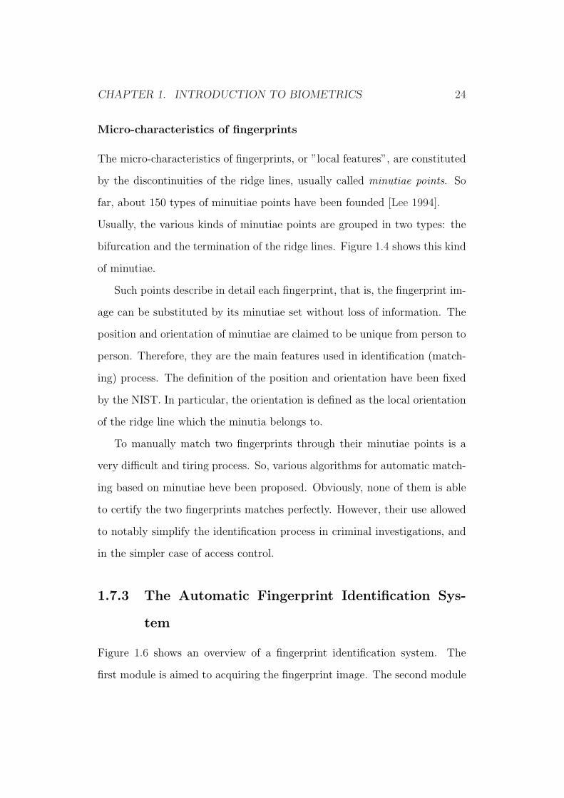
Micro-characteristics of fingerprints
The micro-characteristics of fingerprints, or ”local features”, are constituted
by the discontinuities of the ridge lines, usually called minutiae points. So
far, about 150 types of minuitiae points have been founded [Lee 1994].
Usually, the various kinds of minutiae points are grouped in two types: the
bifurcation and the termination of the ridge lines. Figure 1.4 shows this kind
of minutiae.
Such points describe in detail each fingerprint, that is, the fingerprint im-
age can be substituted by its minutiae set without loss of information. The
position and orientation of minutiae are claimed to be unique from person to
person. Therefore, they are the main features used in identification (match-
ing) process. The definition of the position and orientation have been fixed
by the NIST. In particular, the orientation is defined as the local orientation
of the ridge line which the minutia belongs to.
To manually match two fingerprints through their minutiae points is a
very difficult and tiring process. So, various algorithms for automatic match-
ing based on minutiae heve been proposed. Obviously, none of them is able
to certify the two fingerprints matches perfectly. However, their use allowed
to notably simplify the identification process in criminal investigations, and
in the simpler case of access control.
1.7.3 The Automatic Fingerprint Identification Sys-
tem
Figure 1.6 shows an overview of a fingerprint identification system. The
first module is aimed to acquiring the fingerprint image. The second module

CHAPTER 1. INTRODUCTION TO BIOMETRICS 25
Figure 1.6: The Automatic Fingerprint Identification System (AFIS) scheme

CHAPTER 1. INTRODUCTION TO BIOMETRICS 26
typically enhances the quality of the acquired image. The third module
performs the preliminary classification of the fingerprint, i.e., it assign a
class among those viewed in section 1.7.2. The fourth module is the matching
module. It performs a comparison between the input fingerprint and the ones
stored in the fingerprint database and associated to the class(es) computed
by the classification module.
The output of the matching module is a score, i.e. a similarity degree from
the compared fingerprints. Such score can be used in two ways:
• if the identification one to one is performed, such score has been derived
from the comparison between the given fingerprint and the template
fingerprint associated to the claimed identity. In other words, the per-
son to be recognised by-passes the classification module by declaring
his/her identity. In this case, if the score exceeds a certain fixed accep-
tance threshould, the claimed identity is ”verified”).
• if the identification one to many is perfomed, the score value is associ-
ated to a certain identity. By ordering the identities in fuctions of the
increasing order of their score, the system returns the most probable
identities which the inpunt fingerprint belongs to).
This thesys study deeply the classification module used for the identifica-
tion one to many. We investigate novel algorithms to fingerprint classification
and their fusion, whether among themselves or among other important ap-
proaches proposed in literature. Next chapter describes the state of the art of
fingerprint classification approaches, with particular attention to statistical
and structural ones.

Chapter 2
Fingerprint Classification:
State of Art
The simplest way to classify a fingerprint is to localise their core and delta
points. By counting the number of such singularities, it is possible to identify
the class which the fingerprint belongs to. Karu and Jain [Karu 1996] present
a simple classification system based on such computation. Unfortunately, this
approach does not work well if the image is significantly corrupted by the
noise, that does not allow to reliably localize the singularities points.
Due to the above limitations, the most of the proposed approaches to
automatic fingerprint classification are only partially based on the singular-
ities detection (e.g., on the detection of the core point), and try instead to
extract global features related to the ridge flow orientations. To this end,
many classification algorithms compute the so-called orientation field, which
is the map of the ridge-flow average orientations of the fingerprint image.
Figure 2.1 shows an example of orientation field extracted from a fingerprint
image.
27

CHAPTER 2. FINGERPRINT CLASSIFICATION: STATE OF ART 28
Figure 2.1: Example of fingerprint image and corresponding orientation field.
In the example, the original image is 480x512 pixels sized. Each pixel of the
orientation field has been computed with a 32x32 pixels sized block of the
original image, so generating a 28x30 pixels sized orientation field
So far, many approaches for fingerprint classification have been proposed.
They are based on different pattern recognition teories. Main approaches are:
• Statistical methods: are based on the identification of singular points
(core and delta points). The used criteria for singularities computing
are assentially euristics and the success for finding them is strongly
affected by noise. In fact, in the cases in which the noise is very high,
it is possible to not take delta or core points, or take them in incorrect
positions. This kind of methods transform patterns in a features vector
of fisical and real characteristics.
• Geometrical methods: are based on geometrical approssimation of
the ridge. As an example, we mention the method of Ghong [Ghong 1997]
that use the B-splines.
• Syntactical methods: among the first methods devised, they date
from the Seventies. The basic idea consists in associate at each class
a grammar that describes the fingeprint. Each fingerprint is coded as

CHAPTER 2. FINGERPRINT CLASSIFICATION: STATE OF ART 29
a phrase. Then a syntactical analysis is performed and finally it is
associated to the grammar of which the phrase respects the rules, that
is, the fingerprint is classified.
• Structural methods: innovative methods that exploit the structure
of the pattern and trasform them in structural data.
• Neural methods: methods that exploit a neural network as finger-
print classifier. A neural network can be a simple perceptron, a multi-
layer perceptron (MLP) or a more complex architecture as a recursive
neural network (RNN).
For the purposes of this work, the proposed approaches to fingerprint
classification can be subdivided into the two main categories of statistical
and structural approaches.
Statistical methods are characterised by the use of the decision-theoretic ap-
proach to pattern classification [Duda 2001], namely, a set of characteristic
measurements, called feature vector, is extracted from fingerprint images and
used for classification [Candela 1995]-[Yao 2003].
Structural approaches basically use the syntactic or structural pattern recog-
nition methods [Moayer 1975]-[Neuhause 2005]. Fingerprints are described
by production rules or relational graphs, and parsing processes or graph
matching algorithms are used for classification.
Recently, the fusion of multiple fingerprint classifiers has been proposed
[Yao 2003], [Senior 2001]-[Neuhause 2005 b].

CHAPTER 2. FINGERPRINT CLASSIFICATION: STATE OF ART 30
2.1 Statistical methods
Statistical methods use a vector of statistical measures to represent the fin-
gerprints. In [Ghong 1997] the sequence of the B-splines coefficients was used
in order to approximate the orientation field, i.e. the orientation of the skin
ridge flow, and an empirical rule is used to perform the final classification.
In [Candela 1995] the researchers of the National Institute of Standard and
Technology (NIST) proposed a method based on the KL-transform of the
orientation field (the representation of the fingerprint). A probabilistic Neu-
ral Network is used for elaborating the obtained pattern and for making the
final classification.
In [Jain 1999 b] each fingerprint is described in terms of fingercode. We de-
scribe this method with more details because we used it for comparison and
fusion with our methods. The core of such approach is a novel representation
scheme (called ”FingerCode”) which is able to represent into a numerical
feature vector both the minutiae details and the global ridge and furrows
structures of fingerprints. The computation of such FingerCode starts by
identifying the ”core” point in the fingerprint input image and by defining a
spatial tessellation of the image region around this point. This spatial tessel-
lation is a circle decomposed in 48 sectors. Then, four band-pass Gabor filters
with orientation-selective characteristics (00, 450, 900, and 1350) are applied
to such tessellated image, so producing four orientation-filtered images. Each
filtered image accentuates ridge structures along one orientation. Finally, for
each filtered image and for each sector, the standard deviation of grey level
values is computed, and the FingerCode feature-vector with 192 elements is
produced. Jain and his collaborators used such feature vector as input to
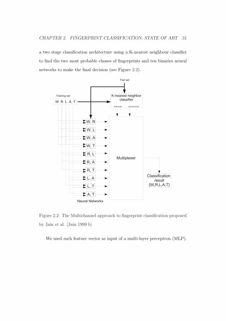
CHAPTER 2. FINGERPRINT CLASSIFICATION: STATE OF ART 31
a two stage classification architecture using a K-nearest neighbour classifier
to find the two most probable classes of fingerprints and ten binaries neural
networks to make the final decision (see Figure 2.2).
Figure 2.2: The Multichannel approach to fingerprint classification proposed
by Jain et al. [Jain 1999 b]
We used such feature vector as input of a multi-layer perceptron (MLP).

CHAPTER 2. FINGERPRINT CLASSIFICATION: STATE OF ART 32
2.2 Structural and graph-based methods
The structural approaches describe the fingerprint in terms of grammars or
graphs.
Moayer and Fu (1975) [Moayer 1975] and Rao and Balk (1980) [Rao 1980]
give a syntactical description of the fingerprint, by defining a set of terminal
symbol, based on the ”local structure” of the skin ridges, and a set of produc-
tion rules to create a grammar that represents each class. A parsing algorithm
is applied to perform the final classification. These kind of approaches are
the oldest, and they have been dropped by the modern research, because
of their sensitivity to the noise frequently added to the fingerprint images
during the acquisition process.
In Cappelli et al (1999) [Cappelli 1999] an adaptative filter, called ”dy-
namic mask” and correspondent to each class is applied to the orientation
field in order to segment it. In the following we describe deeply this method
because we use it for comparison and fusion with our ones.
This method was introduced to overcome the large variability of segmenta-
tions of similar fingerprints, which comes out when the segmentation algo-
rithm described in [Maio 1996] is applied. The basic idea of this approach is
to perform a ”guided” segmentation of the orientation field of the fingerprint
image in order to reduce the variability during the segmentation process.
To this end, five filters, called ”dynamic masks”, one for each class, ”guide”
the orientation field segmentation, so producing a class-dependent segmen-
tation. Such dynamic masks can be regarded as ”prototypes” of images
segmented by the orientation field. Using these filters the number of seg-
CHAPTER 2. FINGERPRINT CLASSIFICATION: STATE OF ART 33
mentation regions and the coarse region shape are fixed. Each dynamic
mask is obtained by the following four steps:
1. for each class, selection of a set of representative fingerprints
2. computation of the respective orientation fields
3. application of a genetic algorithm to segment the orientation field
4. identification of an ”average” ensemble of fixed and mobile vertices and
segments that define the mask. Such vertices are located around the
singularity points (”core” and ”delta”)
To classify fingerprints, the orientation field of an input fingerprint is seg-
mented according to the five dynamic masks (one for each class). For each
mask, a ”cost” provides a measure of the difficulty of the guided segmen-
tation process. Accordingly, the lowest cost means that the segmentation
process can easily produce a segmented image very similar to the used mask.
The cost vector is then converted into a posterior probabilities vector. The
class associated to the maximum posterior probability is associated to the
fingerprint.
In Lumini et al. (1999) [Lumini 1999] the orientation field of a given fin-
gerprint image is computed. A segmentation is performed in order to parti-
tion the orientation field in ”homogeneous orientation” regions. A relational
graph is defined by starting from the segmentation. Finally an unelastic
matching with a template graph for each class is performed and the best
match determines the final classification.
In Yao et al. (2003) [Yao 2003] the fingerprint is described by a Directed
Oriented Acyclic Graph, and a structural vector is extracted from the given

CHAPTER 2. FINGERPRINT CLASSIFICATION: STATE OF ART 34
graph and merged with the ”fingercode” of the original image. A set of Sup-
port Vector Machines (SVMs) is trained and the outcomes of each classifier
are combinated through an Error Correcting Output Code System, in order
to make the final decision. This system presents a better accuracy rejection
curve with respect to that reported in [Jain 1999].
Senior [Senior 2001] proposes a fingerprint classification system based on
the integration of hidden markov models (HMM) and decision trees (DT).
The HMM-based classifier is trained by a set of novel features extracted from
the skin ridge flow. Such feature extraction step is performed as follows.
A set of horizontal and vertical ”fiducial” lines intersects the skeletonised
fingerprint image at different locations. At each ’fiducial line’-’ridge line’
intersection, a set of measures is computed. A multi-layered HMM is designed
by considering the so-computed set of features at each fiducial line as the
input of each layer. The decision tree classifier is trained on another set
of features extracted from the skin ridge flow. Such features are aimed to
encode the ridge shape. The outcomes of the DT and HMM classifiers are
the inputs of a feed-forward neural network for the final classification.
A graph matching based approach using directional variance is recently
proposed by Neuhause and Bunke (2005) [Neuhause 2005]. It consists on
computation of a directional variance measured at each pixel of orientation
field. The variance is defined such that high variance areas correspond to
relevant regions to discriminate between fingerprint Henrys classes. These
regions are not only singular points, but also areas with vertical ridge orienta-
tion. The resulting structures are converted into attributed graphs. A node
corresponds to a pixel of the selected high variance regions and the edges are

CHAPTER 2. FINGERPRINT CLASSIFICATION: STATE OF ART 35
the connection among the pixel. The attributes are the position of the corre-
sponding pixel as node feature and an angle information as edge feature. In
order to perform the classification, a K-Nearest Neighbour paradigm is ap-
plied. The edit distance is based on a simple cost function in which constant
costs are assigned to insertion and deletion operations and a value propor-
tional to the Euclidean distance of attributes is assigned to costs of substi-
tution operations. In order to find the minimum path for the edit distance,
only a subset of all edit paths is considered in the approximate algorithm,
instead of exploring the full search space. The prototypes set is established
by manually selecting promising candidates. It consists of 60 elements.
2.3 Multiple classifiers system to fingerprint
classification
So far, the works [Jain 1999], [Yao 2003], [Cappelli 2002], [Nagaty 2001] and
[Neuhause 2005 b] are the only ones in which a multiple classfier system is
used for the performance improvement. In particular, [Cappelli 2002] use the
”dynamic masks” method as first classifier.
Moreover, a novel transformation of the orientation field, called Multiple KL-
tranform (MKL), generates a feature vector for each fingerprint. Two clas-
sifiers (Nearest Neighbour and a K-Nearest Neighbour) are trained by using
the MKL transformation, and the decisions of the Dynamic Mask method
and the two classifiers described above are finally combined by using the ma-
jority voting rule [Windeatt 2003].
Nagaty (2001) [Nagaty 2001] proposed the combination between statistical

CHAPTER 2. FINGERPRINT CLASSIFICATION: STATE OF ART 36
and structural features at the level extraction. The structural features are
represented by the orientation field codified into a binary string of fixed di-
mension. The statistical features are represented by a ”texture measure”
performed by the computation of the second moments. A feature vector
made up of the whole statistical and structural features (186 features) is the
input of a Artificial Neural Network which performs the final classification.
A very recent work is proposed by Neuhause [Neuhause 2005 b]. The fusion is
performed by generating a unique graph from different graph representations
of each pattern. Each representation is obtained by different approaches.
For each pattern, the two most similar graphs are searched for, then they
are merged to obtain one graph. The process iteratively continues until all
graphs are reduced in only one graph.
Chapter 3
A Graph-Based Approach to
Fingerprint Classification
3.1 Introduction
Fingerprint classification is based on the shape described by the skin ridges
flow of such biometrics: Arch (A), Tended Arch (T), Left Loop (L), Right
Loop (R) and Whorl (W). The next step is to recognise the fingerprint by
performing a search in the set of fingerprints associated to the identified class
(matching process). This strategy is necessary for reducing the identification
time.
Unfortunately, fingerprint classification task is made very difficult by sev-
eral factors. Among the others, the poor quality of real fingerprint images
which can decease the singularity points detection, and the existence of am-
biguous fingerprints which cannot be reliably classified even by human ex-
perts. In particular, the crucial issue of ambiguous fingerprints is due to the
large within-class variability and the small between-class separation. In some
37

CHAPTER 3. GRAPH-BASED APPROACH 38
cases, fingerprints which cannot be reliably assigned to a single class even by
human experts are labelled with two classes, and named ”cross-referenced”
fingerprints. These fingerprints are so called because two classes, instead of
one, are associated to them. Figure 3.1 shows an example of ”AT cross-
referenced” fingerprint, beside a A and a T fingerprint. Because of the shape
”continuity” among classes, it is impossible to associate only one of them.
Figure 3.1: Example of AT cross referenced fingerprint compared with A and
T fingerprint images
As said in Chapter 2, the proposed approaches to automatic fingerprint
classification can be coarsely subdivided into two main categories of ”flat”
and ”structural” approaches. Flat approaches are characterised by the use
of the ”decision theoretic” or statistical approach to pattern classification,
namely, a set of characteristic measurements, called feature vector, is ex-
tracted from fingerprint images and used for classification ([Candela 1995],
[Jain 1999], [Nagaty 2001], [Senior 2001], [Cappelli 2002]). On the other
hand, structural approaches presented in the literature basically use the syn-
tactic or structural pattern recognition methods ([Moayer 1975], [Rao 1980],
[Cappelli 1999], [Lumini 1999], [Yao 2003], [Neuhause 2005 b]). Fingerprints
are described by production rules or relational graphs and parsing processes
or graph matching algorithms are used for classification. It is worth re-
CHAPTER 3. GRAPH-BASED APPROACH 39
marking that the structural approaches of fingerprint classification has not
received much attention still now. However, a simple visual analysis of the
structure of fingerprint images allows one to see that structural information
can be very useful for distinguishing fingerprint classes of the arch and whorl
type. On the other hand, it is easy to see that structural information is
not appropriate for distinguishing fingerprint classes of the right loop, left
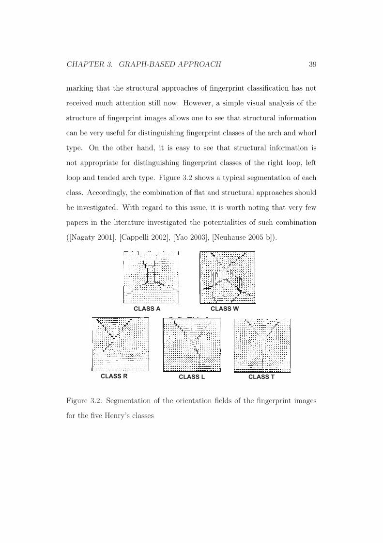
loop and tended arch type. Figure 3.2 shows a typical segmentation of each
class. Accordingly, the combination of flat and structural approaches should
be investigated. With regard to this issue, it is worth noting that very few
papers in the literature investigated the potentialities of such combination
([Nagaty 2001], [Cappelli 2002], [Yao 2003], [Neuhause 2005 b]).
Figure 3.2: Segmentation of the orientation fields of the fingerprint images
for the five Henry’s classes

CHAPTER 3. GRAPH-BASED APPROACH 40
3.2 An appropriate data representation
According to section 1, our definition of fingerprint structure corresponds to
the topology of completely connected ”regions” grouping ridges and valleys
with homogenous orientations. Such topology relies on the singularities lo-
cations. Hence, it is different from class to class, according to the Henry’s
classification [Henry 1900].
The so defined fingerprint structure can be easly extracted by segmenting
the fingerprint orientation field into regions characterised by homogeneous
ridge directions ([Yao 2001], [Yao 2003], [Lumini 1999], [Cappelli 1999],
[Marcialis 2001], [Marcialis 2003]).
The first problem is how to describe such structure through an appropri-
ate data type. The relational graph appears to be an appropriate type of
data for describing the fingerprint topology. The relational graph nodes could
correspond to regions extracted by the segmentation algorithm, as shown in
[Lumini 1999]. However, the main arising issue is to find the best represen-
tative graph for each fingerprint class, in order to apply a template-matching
algorithm, like such shown in figure 3.3. In particular, L, R and T classes,
fingerprints structures are very difficult to separate by a simple relational
graph-based representation.
The second problem is to make the above fingerprint representation ”ro-
bust” to the large small-within class variability and the small between-class
variability, which is accentuated in real applications because of the noise in
sensed data. Because each region derives from the segmentation algorithm,
the robustness degree is mainly dependent on such algorithm. However, to
the best of our knowledge, none of the proposed segmentation algorithms
CHAPTER 3. GRAPH-BASED APPROACH 41
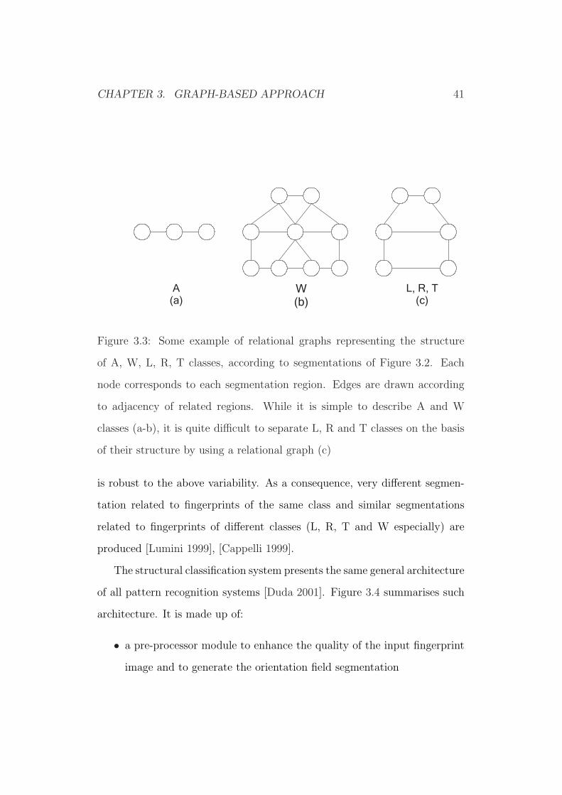
Figure 3.3: Some example of relational graphs representing the structure
of A, W, L, R, T classes, according to segmentations of Figure 3.2. Each
node corresponds to each segmentation region. Edges are drawn according
to adjacency of related regions. While it is simple to describe A and W
classes (a-b), it is quite difficult to separate L, R and T classes on the basis
of their structure by using a relational graph (c)
is robust to the above variability. As a consequence, very different segmen-
tation related to fingerprints of the same class and similar segmentations
related to fingerprints of different classes (L, R, T and W especially) are
produced [Lumini 1999], [Cappelli 1999].
The structural classification system presents the same general architecture
of all pattern recognition systems [Duda 2001]. Figure 3.4 summarises such
architecture. It is made up of:
• a pre-processor module to enhance the quality of the input fingerprint
image and to generate the orientation field segmentation

CHAPTER 3. GRAPH-BASED APPROACH 42
• graph generator module, which takes as input the orientation field seg-
mentation provided by the previous module. Each node of the graph is
enriched by a real-valued feature vector extracted from the orientation
field. We used two graph representation; a generic relational graph and
a DPAG, namely, Directed Acyclic Positional Graph.
• an appropriate machine learning model for each data representation: a
classical graph-based classifier, based on inexact graph matching theory
and a Recursive Neural Network for classifying the fingerprint. These
methods takes as input the graph representation generated by the pre-
vious module, respectively.
Figure 3.4: Modules of our fingerprint classification system
3.3 The pre-processor module
The pre-processor module performs the enhancement, the orientation com-
putation and the segmentation of the fingerprint image, as shown in Figure
CHAPTER 3. GRAPH-BASED APPROACH 43
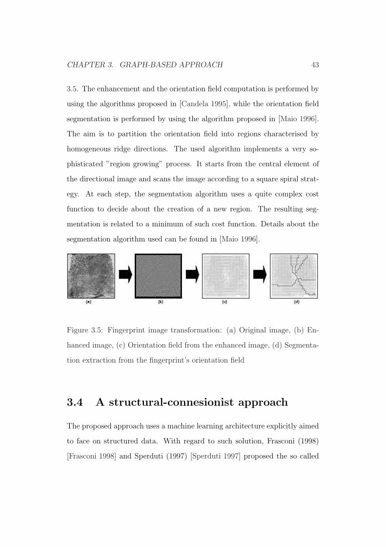
3.5. The enhancement and the orientation field computation is performed by
using the algorithms proposed in [Candela 1995], while the orientation field
segmentation is performed by using the algorithm proposed in [Maio 1996].
The aim is to partition the orientation field into regions characterised by
homogeneous ridge directions. The used algorithm implements a very so-
phisticated ”region growing” process. It starts from the central element of
the directional image and scans the image according to a square spiral strat-
egy. At each step, the segmentation algorithm uses a quite complex cost
function to decide about the creation of a new region. The resulting seg-
mentation is related to a minimum of such cost function. Details about the
segmentation algorithm used can be found in [Maio 1996].
Figure 3.5: Fingerprint image transformation: (a) Original image, (b) En-
hanced image, (c) Orientation field from the enhanced image, (d) Segmenta-
tion extraction from the fingerprint’s orientation field
3.4 A structural-connesionist approach
The proposed approach uses a machine learning architecture explicitly aimed
to face on structured data. With regard to such solution, Frasconi (1998)
[Frasconi 1998] and Sperduti (1997) [Sperduti 1997] proposed the so called

CHAPTER 3. GRAPH-BASED APPROACH 44
”Recursive Neural Networks” (RNNs). By using this machine learning ar-
chitecture, we avoid the problem to design a set of templates for each class,
because Recursive Neural Networks are specialised in learning to classify
complex data structures by examples.
The main limitation of such approach is that RNNs can learn to classify
only data structures in terms of Directed Positinal Acyclic Graphs (DPAGs).
A DPAG is a directed acyclic graph in which the ”children-nodes” (the nodes
linked by another node, also called ”father-node”) are ordered according to a
certain rule. As an example, a node of the DPAG can have the first child, the
second child, the fourth child, while the third one is missed. In a DPAG for
classification by RNNs, (a) the maximum number of children-nodes, called
”out-degree”, is given; (b) the ”super-source” node is also defined as the
node which connects all nodes of the graph, by following a directed path
[Frasconi 1998].
It is evident that the use of a DPAG implies some topological constraints
which could determine the loss of information in describing the fingerprint
structure. In particular, the DPAG could not take into account all segmen-
tation regions because of the designed positional rule between children-nodes
and father-node. So, a DPAG generation algorithm could be not able to pre-
serve the original fingerprint segmentation topology. In order to reduce such
possible loss of information, a DPAG generation algorithm addressing such
issue is needed [Yao 2003]. The DPAG based representation of fingerprints is
then completed by attaching to each graph node some local characteristics of
regions and some geometrical and spectral relations among adjacent regions.

CHAPTER 3. GRAPH-BASED APPROACH 45
3.4.1 The directional positional acyclic graph genera-
tor module
The main rational behind of our DPAG generation algorithm is
1. to associate a segmentation region to each graph node
2. to draw the completed connected relational graph on the basis of the
adjacencies amog regions (i.e. a graph edge connects only adjacent
regions)
3. to cut the edges responsible of cycles in the graph on the basis of a
hierarchical rule defining the starting node (the super-source), its child
nodes and so on.
A rule for ordering the child-nodes is also necessary to obtain a DPAG.
In designing such rules, it is necessary to preserve as more as possible the
topology of the orientation field segmentation.
The DPAG-based fingerprint description is then completed by attaching
to each node a feature vector containing local characteristics of the related
region and by geometrical and spectral relations among adjacent regions.
In the following, we describe the algorithm for DPAG generation from the
orientation field segmentation and then we describe the features attached to
each graph node.
DPAG generation from the orientation field segmentation
It is presented a DPAG generation algorithm from orientation field segmen-
tations in [Yao 2001], [Yao 2003] and [Marcialis 2001], before our generation

CHAPTER 3. GRAPH-BASED APPROACH 46
algorithm. Briefly, such previous algorithm describes the segmentation topol-
ogy starting from the region containing the core point. The positional rule
between father-node and children-nodes is as follows: 8 positions are consid-
ered (8 is the DPAG out-degree), each of them corresponds to the relative lo-
cation of the child-node with respect to the father-node (North, North-East,
East, South-East, South, South-West, West, North-West). Such locations
are computed in according to their baricenters relative positions. As an ex-
ample, if the child-node baricenter is to North of the father-node baricenter,
the position ”North” is assigned to such child node; when the child node
baricenter is to North-East, the position ”North-East” is assigned and so on.
The main drawbacks of such algorithm are that:
1. if more than one child-node concur to the same position with respect
to the same father-node, some of such nodes could be lost during the
DPAG generation, so producing a DPAG generation failure (we called
such nodes ”orphans-nodes”)
2. the core point could not be found at all in certain images, so producing
failure in the core detection.
As a consequence of both cases, the fingerprint is rejected because it cannot
be make reliable and suitable for the RNN processing. In particular, the first
issue indicates that such algorithm is not always able to preserve the original
fingerprint topology.
Accordingly, we designed the following algorithm to address such issues.
The complete algorithm is presented in the pseudo-code form in Figure 3.6.
Figure 3.7 shows an example of DPAG generation with the proposed
algorithm. The proposed algorithm can be summarised as follows:

CHAPTER 3. GRAPH-BASED APPROACH 47
Figure 3.6: Pseudo-code of the DPAG generation algorithm
• The whole orientation field image is the super-source S
• The regions of the segmented orientation field image are first ordered
according to the relative positions of the centre of mass
• The first region R1 is assigned as the first child of the super-source

CHAPTER 3. GRAPH-BASED APPROACH 48
• The sub-image starting from the x-coordinates of the R1’s centre of
mass is partitioned in od rectangles, where od is the out-degree of the
DPAG. Figure 3.7 shows an example of such rectangles starting from
the region labelled with ”0”. Figure 3.7 also shows the center of mass
of the regions by little filled circles. In the example, od = 8
• The first baricenter belonging to an adjacent region of R1, found in the
i-th rectangle, is assigned as the i-th child of the node associated to R1
• The same process is repeated for the children-nodes while all regions
have been considered
It is easy to see that this process allows to avoid the presence of cycles in
the graph. However, it may be happen that a node may be assigned as child
of any DPAG’s node. In order to take into account these nodes, we simply
attached them to the super-source S (the whole orientation field image) by
considering them as ”super-source children” in the positions od + 1, od + 2
and so on, according to their order. Consequently, the DPAG out-degree is
od + N , being N the number of segmentation regions.
The above algorithm does not present the drawbacks of the previous one
[Yao 2003] because:
• it avoids the issue of the nodes loss by introducing the ordered rule for
recovering the orphans-nodes
• it avoids the dependence of the starting point on the fingerprint core
detection
It is also worth noting that the fingerprint topology preserved by the proposed

CHAPTER 3. GRAPH-BASED APPROACH 49
Figure 3.7: Example of DPAG generated from the orientation field image.
The out-degree is 8. In this example, the region ’0’ has the baricenter at
the position {x = 7, y = 10}. According to the algorithm of Figure 8, this
is the first child of the super-source S (the whole image). Then, the sub-
image starting from the x-coordinate of the baricenter of ’0’ is partitioned
in 8 rectangles labelled from 0 to 7. The baricenter of Region ’1’ is located
in the rectangle no.1. Being Region ’1’ adjacent to Region ’0’, Region ’1’ is
assigned as the child no.1 of Region ’0’, as it can be seen from the label of
the related arch of the DPAG
algorithm, because it takes into accunt all regions. So, it is possible to
averagely recover the original segmentation topology.

CHAPTER 3. GRAPH-BASED APPROACH 50
Feature extraction for the DPAG representation
The representation is completed by characterising the nodes with local fea-
tures and relational features with children-nodes. The first ones are:
• Mean and standard deviation of the region orientations
• Baricenter-coordinates and area of the region. Area’s value is nor-
malised with respect to the area of overall image.
• Distribution of the orientation field in the image, in terms of probability
of a certain orientation value given the region. Eight orientation values
were considered in the range [jπ/4, (j +1)π/4], where j = 0, . . . , 7, and
the number of pixels of the orientation field of the region that fall in
each interval was computed. In the following, we indicated this number
with cj, related to the j-th interval. For estimating the probability, each
value was normalised with respect to the area of the region. Hence, for
each region (node):
pj =cj
A
• ”Cumulative” distribution of the orientation field. For each node, the
following feature is defined: cumj(v) = cj(v) +∑
u∈Children(v) cj(u),
where Children(v) is the set of ordered v’s children nodes. In the case
of a leaf-node: cumj(v) = cj(v). The normalisation with respect to the
sum of the node areas is performed:
pcumj(v) =
cumj(v)
A(v) +∑
u∈Children(v) A(u)
The relational features are ”distance” values:

CHAPTER 3. GRAPH-BASED APPROACH 51
• Among the baricenters
• Among the means and among the standard deviations
• Among the distributions of the orientation field of different regions.
Named d(u, v) this distance:
d(u, v) =∑
j
|pj(v)− pj(u)|
where u ∈ Children(v)
• We computed the perimeter of adiacency among two adiacent regions
• We also computed a modified version of the Mahalanobis distance for
characterising the relationship among means and standard deviations
of different regions. Named µf and σf the mean and the standard
deviation of the orientations of the father-node, and named µc and σc
the mean and the standard deviation of the orientations of the child-
node, we defined:
d(Rf , Rc) =(µf − µc)
2
σfσc
3.4.2 Recursive neural networks for fingerprint class-
fication
Research in connessionist models capable of representing and learning struc-
tured (or hierarchically organised) information begun in the early 90’s with
recursive auto-associative memories (RAAM) [Pollack 1990]. Since then, sev-
eral other architectures have been proposed, including holografic reduced
representation (HRR) [Plate 1995], and Recursive Neural Networks (RNN)
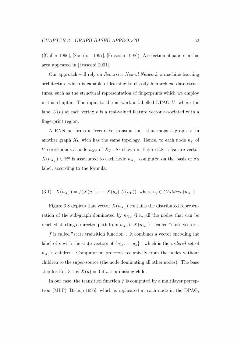
CHAPTER 3. GRAPH-BASED APPROACH 52
([Goller 1996], [Sperduti 1997], [Frasconi 1998]). A selection of papers in this
area appeared in [Frasconi 2001].
Our approach will rely on Recursive Neural Network, a machine learning
architecture which is capable of learning to classify hierarchical data struc-
tures, such as the structural representation of fingerprints which we employ
in this chapter. The input to the network is labelled DPAG U , where the
label U(v) at each vertex v is a real-valued feature vector associated with a
fingerprint region.
A RNN performs a ”recursive transduction” that maps a graph V in
another graph XV wich has the same topology. Hence, to each node nV of
V corresponds a node nXVof XV . As shown in Figure 3.8, a feature vector
X(nXV) ∈ <n is associated to each node nXV
, computed on the basis of v’s
label, according to the formula:
X(nXV) = f(X(u1), . . . , X(uk), U(nV )), where uj ∈ Children(nXV
)(3.1)
Figure 3.8 depicts that vector X(nXV) contains the distributed represen-
tation of the sub-graph dominated by nXV(i.e., all the nodes that can be
reached starting a directed path from nXV). X(nXV
) is called ”state vector”.
f is called ”state transition function”. It combines a vector encoding the
label of v with the state vectors of {u1, . . . , uk} , which is the ordered set of
nXV’s children. Computation proceeds recursively from the nodes without
children to the super-source (the node dominating all other nodes). The base
step for Eq. 3.1 is X(u) = 0 if u is a missing child.
In our case, the transition function f is computed by a multilayer percep-
tron (MLP) [Bishop 1995], which is replicated at each node in the DPAG,

CHAPTER 3. GRAPH-BASED APPROACH 53
Figure 3.8: A recursive transduction from a simple input DPAG (outdegree =
2) to the state-DPAG labelled with state vectors. The node labelled with
the state vector X(S) contains the distributed representation of the whole
input DPAG. Each child can be univocally identified through its position
with respect to the father: e.g., A is the first child of S, B the second. It is
worth noting that C has not children. In this case, the base-step is applied
for each missing child
sharing weights among replicas. Classification with recurrent neural networks
is performed by adding an output function g that takes as input the hidden
state vector X(s) associated with the super-source s:
Y = g(X(s)
)(3.2)
It is worth noting that X(s) can be extracted and independently used as
a ”structural” feature vector, because it contains the distributed represen-
tation of the whole DPAG. Function g is also implemented by a multilayer
perceptron.
The output layer in this case uses the softmax functions (normalised expo-
nentials), so that Y can be interpreted as a vector of conditional probabilities
of classes given the input graph, i.e. Yi = P (C = i|V ) , being C a multi-

CHAPTER 3. GRAPH-BASED APPROACH 54
nomial class variable [Bishop 1995]. Training relies on maximum likelihood.
The training set consists of T pairs
D ={(
U1, c(U1)), . . . ,
(Ut, c(Ut)
), . . . ,
(UT , c(UT )
)}(3.3)
where c(Ut) denotes the class of the t-th fingerprint in the data set. Ac-
cording to the multinomial model, the log-likelihood has the form:
l(D; Θ) =∑
t
logYc(Ut)(3.4)
where Θ denotes the set of trainable weights and t ranges over training
examples. Optimisation is performed with a gradient descent procedure,
where gradients are computed by the Back-Propagation Through Structure
algorithm [Sperduti 1997].
In order to take into account the cross-referenced fingerprints, charac-
terised by two classes instead of one, a ”soft” target vector was introduced
in the training phase. The two cross-referenced classes were considered to
have the same probability given the pattern. Thus, the target-vector takes
value 0.5 in correspondence of the two target classes of the cross-referenced
fingerprints. For the standard fingerprints, the target-vector takes value 1.0
in correspondence of the target class.
3.5 The structural K-nn approach
One of the most natural structural representation of the fingerprint orienta-
tion field segmentation (i.e., of the segmentation of the fingerprint image in
regions with homogeneous orientation of ridge and valley, as shown in Fig-
ure 3.2) is a relational graph. Relational graphs appear to be appropriate,

CHAPTER 3. GRAPH-BASED APPROACH 55
as nodes could naturally correspond to the regions extracted by the seg-
mentation algorithm [Lumini 1999]. Each graph node can be associated to a
segmentation region and the edges join two nodes according to the adjacency
relationship of the respective regions.
Figure 3.9 shows an example of relational graph related to a fingerprint
orientation field segmentation.
Figure 3.9: Graph-based representation obtained from the segmented orienta-
tion field of a fingerprint image. Node labels represent the number associated
to each region as shown in the orientation field and the edge labels represent
the position of each child-node
The representation is completed by associating to each node a feature
vector containing the local characteristics of the regions (area, average direc-
tional value, etc) and the geometrical and spectral differences among adjacent
regions (relative positions, differences among directional average values, etc).
A graphical representation of this kind of graph is shown in Figure 3.10.
Graph matching is a method to perform structural data classification.
The graph matching we used is based on the computation of the graph edit
distance between the input graph and a set of prototype graphs representing
each class. It works such as the K- nearest neighbor classifier but the distance

CHAPTER 3. GRAPH-BASED APPROACH 56
Figure 3.10: A generic attributed graph. Node labels represent the number
associated to each region as shown in the orientation field and the edge labels
represent the position of each child-node
between input patterns and prototypes, since the patterns are represented by
graphs, is the edit distance, that is, a particular measurement of differences
between two graphs. Therefore, distances between input graph and model
graphs are computed; then, the class associated to the input graph is the
most represented in the nearest K prototypes to the input graph.
Figure 3.11: K nearest neighbors representation in a space in which can be
represented graphs. The distance between graph patterns is edit distance,
i.e. a measurement of difference between two graphs
Edit distance is the minimum cost obtainable by applying edit opera-
tions, i.e. node/edge substitution, in order to transform an input graph to a
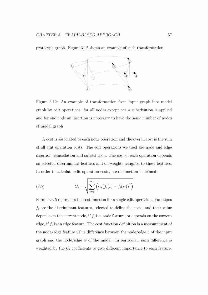
CHAPTER 3. GRAPH-BASED APPROACH 57
prototype graph. Figure 3.12 shows an example of such transformation.
Figure 3.12: An example of transformation from input graph into model
graph by edit operations: for all nodes except one a substitution is applied
and for one node an insertion is necessary to have the same number of nodes
of model graph
A cost is associated to each node operation and the overall cost is the sum
of all edit operation costs. The edit operations we used are node and edge
insertion, cancellation and substitution. The cost of each operation depends
on selected discriminant features and on weights assigned to these features.
In order to calculate edit operation costs, a cost function is defined.
(3.5) Ce =
√√√√Nf∑i=1
(Ci
(fi(v)− fi(w)
)2)
Formula 3.5 represents the cost function for a single edit operation. Functions
fi are the discriminant features, selected to define the costs, and their value
depends on the current node, if fi is a node feature, or depends on the current
edge, if fi is an edge feature. The cost function definition is a measurement of
the node/edge feature value difference between the node/edge v of the input
graph and the node/edge w of the model. In particular, each difference is
weighted by the Ci coefficients to give different importance to each feature.

CHAPTER 3. GRAPH-BASED APPROACH 58
If cancellation or insertion operation is applied, the feature value related to
the input graph or to the model graph is zero. Then, getting simpler, the
cost function becomes:
(3.6) Ce =
√√√√Nf∑i=1
(Cif 2
i (v))
The main issue is to find the sequence of edit operations which provide
the minimum cost. To this aim, a research tree containing all the possible
edit operations sequences is constructed. The search of the best sequence (i.e.
the minimum cost path into the research tree) is performed by an algorithm
similar to A* [Bunke 1983]. This procedure allow to obtain the absolute
minimum cost, namely, allow to find the optimal solution of minimum path
searching problem. The main drawback of such a search in the tree is the
computational complexity in terms of time. Hence, some trick to reduce the
time of computing is applied.
Since there is a Ci coefficient for each feature used, in order to avoid to
select too many Ci, few features are used, the most significant. In particular,
the edit operations cost is based on three node features and only one edge
feature. The following list shows the features selected for each edit operation.
They are a subset of that used for RNNs described in chapter 3.4.
• Node substitution
– Area and baricenter coordinates
– Orientation densities in the 8 main directions
• Node cancellation/insertion
– Area

CHAPTER 3. GRAPH-BASED APPROACH 59
• Edge substitution
– Perimeter of adiacency
• Edge cancellation/insertion
– Perimeter of adiacency
Note that, to have a distance, cancellation and insertion must produce the
same cost, so the related coefficients must be equal. Moreover, edge cancel-
lation may happen in two cases:
1. After node substitution, if doesn’t exist the link between the two sub-
stituted nodes in the model graph
2. After node cancellation, it is necessary to eliminate all edges arriving
in the cancellated node
In order to distinguish these two cases, two different coefficients are used.
Obviously, dual consideration is worth also for edge insertion. So we have
two other different coefficients for edge insertion too.
In order to have outputs for the combination task with other investigated
classifiers, for each test pattern, the mean of K lowest edit distances for each
class is computed and then converted into a posterior probabilities vector.

Chapter 4
Ensembles of Graph Matchers
and Fusion of Structural and
Statistical Fingerprint
Classifiers
The aim of this work is to generate Multiple Classifiers System (MCS) using
structural methods as individual classifiers of the combination system to
classify fingerprints. In particular, we would obtain MCSs automatically from
the same type of classifier. In other words, we would generate an Ensemble of
Graph Matchers. In the literature there are various methods to create MCS
when the individual classifiers are statistical type. On the contrary, so far,
only few approaches with structural individual classifiers have been proposed
(see Section 2.3), and anybody has not yet been proposed an Ensemble of
Graph Matchers for fingerprint classification.
60

CHAPTER 4. ENSEMBLES AND COMBINATIONS 61
First of all, we consider in the section 4.1 the combination with diverse
classifiers for fingerprint classification, i.e. statistical one and different struc-
tural ones. In the section 4.2, we describe how to perform a Multiple Classifier
System for statistical classifiers in order to evaluate either if it is possible to
use the same approaches for structural classifiers or if it is possible to adapt
them. Then, we describe our approaches to design ensembles of structural
matchers.
4.1 Fusion of structural and statistical finger-
print classifiers
In this section, we describe our approach for decision-level fusion of structural
and statistical classifiers. The general scheme is reported in figure 4.1, which
is quite similar to the commonly used multiple classifiers fusion scheme at
the decision-level [Roli 2002].
Figure 4.1: General scheme of a fingerprint classification system
We used the finger-code as statistical representation of the fingerprint
([Jain 1999 b]). This vector is the input of a MultyLayer Perceptron trained
according to the maximum likelihood cost function. The outputs of the net

CHAPTER 4. ENSEMBLES AND COMBINATIONS 62
have the same meaning than those of Recursive Neural Network, Structural
K-nn and Dynamic Masks1, i.e. the estimation of the conditional probability
of each class given the fingerprint pattern with its input features. Hence, the
output of each net is a 5-dimensional vector of probabilities. In the following,
we denote with pRNNc and pMLP
c and so on for the other classifiers, the c-th
outcome of each classifier, representing the probability of the c-th class, given
the pattern (c ∈ {A,L, R, T, W}).Many experimental results heve been shown that classifiers specialised
on different pattern representations can benefit from the fusion of their out-
comes, especially when this information produces ”complementary” classi-
fiers [Roli 2002]. In our case, RNN, MLP Structural K-nn and Dynamic
Masks were trained to classify on diverse information. We studied their com-
plementarity in next chapter.
Accordingly, we assessed two types of fusion algorithm (or ”combination
rules”). The first one was based on a fixed transformation of the outcomes
of the experts. In particular, we used the mean and the product rules:
winnerClass = argmaxc∈{A,L,R,T,W}∑
pic(4.1)
winnerClass = argmaxc∈{A,L,R,T,W}∏
pic(4.2)
where i ∈ {RNN,MLP, SKnn,DMask}, i.e. represents one of the individ-
ual classifiers and it is possible to have combination either with two, three
or all four individual classifiers.
These simple combination rules require the conditional indipendence of
the classfiers given the class, and a strong complementarity, to give optimal
1In our experiments of system combination we used all these strucutral classifiers, as
well as the cited statistical one.

CHAPTER 4. ENSEMBLES AND COMBINATIONS 63
results [Kittler 1998].
The second fusion algorithm followed the so-called ”meta-classification”
(as well as known as ”stacked”) approach which uses an additional classifier
for combination [Giacinto 1997]. In particular, a K-Nearest Neighbors clas-
sifier was used [Duda 2001]. The input of such classifier is a novel feature
vector made up of the outcomes of the expert.
4.2 Ensembles of graph matchers
The fusion of classifiers can happen in different points of classification process.
Figure 4.2 shows that one can fuse at the level of acquisition module when
more than one sensor is utilized. It is the Data Level Fusion. Another
possibility is to fuse at the level of features, manipulating them. The Decision
Level Fusion performs the combination of the outputs of individual classifiers.
At any level the designer wants to work, the aim is to generate complementar
classifiers in order that each base-classifier is competent on a feature space
portion or, in general, on a particular domain. We focused our attention to
the latter level of fusion.
In order to create a multiple classifiers system, different kinds of classifiers
can be considered as base classifiers, like proposed in [Serrau 2005] and in
[Marcialis 2003] for fingerprint classification. In these works statistical and
different types of structural classifiers are combinated at the decision-level
fusion. In order to create automatically different classifiers of the same type,
that is, to create ”Ensembles of classifiers”, one can manipulate training data
or input and output features.
By manipulating training data, one can create through the bootstrap
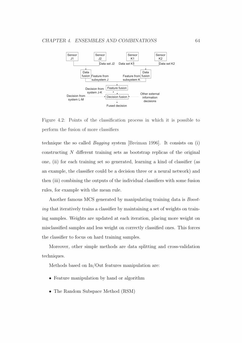
CHAPTER 4. ENSEMBLES AND COMBINATIONS 64
Figure 4.2: Points of the classification process in which it is possible to
perform the fusion of more classifiers
technique the so called Bagging system [Breiman 1996]. It consists on (i)
constructing N different training sets as bootstrap replicas of the original
one, (ii) for each training set so generated, learning a kind of classifier (as
an example, the classifier could be a decision three or a neural network) and
then (iii) combining the outputs of the individual classifiers with some fusion
rules, for example with the mean rule.
Another famous MCS generated by manipulating training data is Boost-
ing that iteratively trains a classifier by maintaining a set of weights on train-
ing samples. Weights are updated at each iteration, placing more weight on
misclassified samples and less weight on correctly classified ones. This forces
the classifier to focus on hard training samples.
Moreover, other simple methods are data splitting and cross-validation
techniques.
Methods based on In/Out features manipulation are:
• Feature manipulation by hand or algorithm
• The Random Subspace Method (RSM)

CHAPTER 4. ENSEMBLES AND COMBINATIONS 65
• Input features can be manipulated by adding noise
• Output features can be manipulated for creating diverse classifiers
(ECOC)
Manual or automatic feature selection can be used for creating different
classifiers using diverse feature sets. It can work if there are features either
redundant or irrilevant. The sets obtained by selecting from the original set,
are subset of that.
The most important method to select features, is the Random Subspace
Method. It consists on selecting a certain number of subspaces from the
original feature space, and training a classifier on each subspace [Ho 1998].
Feature subsets can varying in number and in dimensionality2.
Adding noise to feature space is used to resolve the small sample size
problem that arise when the number of training patterns is smaller than the
feature space dimensionality. It is possible to exploit the noise injection into
input features for creating ensembles that differ in training sets. Usually the
noise distribution is Gaussian, but it can distort data configuration, therefore
it is better injecting noise along the direction of the K nearest neighbors of
each pattern [Skurichina 2000].
Error Correcting Output Coding is a way to manipulate output features.
Each classifier of the multiple system is trained to be competent on a sub-
set of the class set. For example, iteratively partitioning the class set into
two subsets, each classifier has to resolve a binary task. Then, a suitable
combination method able to recover the original classes is necessary, e.g. a
decoding matrix whose rows are the original classes and columns are code-
2Dimensionality of subsets is a critical parameter of the RSM

CHAPTER 4. ENSEMBLES AND COMBINATIONS 66
words associated to each class3.
Finally, one can create multiple classifiers systems by modifying internal
parameters of a certain classifier. As an example, when neural network are
used, its topology and architecture could be modified changing the number of
hidden neurons and/or the number of hidden layers, so generating different
classifiers. In the case of graph-based classifiers, it is possible to exploit
internal parameters such as that used for definition of the distance between
graphs .
4.2.1 Ensembles of statistical vs. structural classifiers
Intuitively, methods that manipulate the training set without operating on
the features, could be applied for create structural MCSs identically to sta-
tistical ones, namely, either Bagging or Boosting, but data splitting or cross-
validation too, if the dataset is enough large. It is not assured that with
these methods a structural classifier can build complementar experts, but
there isn’t any reason that deny it. Therefore, it makes sense trying these
methods. In particular, bagging technique works when base classifiers are ”in-
stable”4. Intuitively, graph-based classifiers are instable, so Bagging should
work if it is applied to a structural classifier.
When MCSs are generated on the basis of features changes, e.g. using the
Random Subspace Method (RSM), the application to structural classifiers is
not trivial. As minimal, it is necessary an extension to treat the feature
3In order to have a good ECOC, row and column separation must be satisfied4As Breiman says in [Breiman 1996], a classifier is instable if, producing small changes
in bootstrap training sets, after learning phase its outputs are very different with respect
to that obtained without introducing changes in the original training set.

CHAPTER 4. ENSEMBLES AND COMBINATIONS 67
vectors labels of each node instead of the classical feature vector, which is
unique for each pattern. For example, we can simply select a subset of the
original node labels, of course, always the same for each node and for each
graph (pattern) for consistency reasons. Another way to do an MCS with
RSM is proposed by [Schenker 2004]: he and their contributors select feature
subsets by randomly removing nodes in each graph. In spite of difficulties
to apply this methods, it seems to be interesting to adapt it for structural
classifiers.
Noise injection also is not a trivial extension to graph-based approaches.
To injecting gaussian noise, it should be applied equally to the features asso-
ciated to each node and edge in order to avoid data configuration distortion.
Moreover, adding noise into the K nearest neighbors direction could be given
for each node or edge. Applying this method to create ensembles seems to
be too much complicate, compared with the few benefits obtainable for the
fingerprint classification task.
As regards the ECOC application, since it involves only the output fea-
tures fusion, should be used without changes or extensions for structural
approaches. Like for statistical classifiers, the critical issue is to find a good
coding.
In conclusion, there is much room to research for ensembles of structural
classifiers and there are very few works about it. In particular, for fingerprint
classification anybody before us has investigated the possibility to expand
ensembles to structural or graph-based methods. In this thesys work we
investigated two of the above mentioned approaches: bagging and internal
parameters variation. We explain these methods in the next section.

CHAPTER 4. ENSEMBLES AND COMBINATIONS 68
4.2.2 Bagging of structural classifiers
As described in section 3.4, the approaches we designed for fingerprint clas-
sification are recursive neural network (section 3.4) and structural K nearest
neighbors (section 3.5). They could be both used as base classifier of bagging,
but for computational complexity reasons, it is not feasible to apply bagging
to structural K-nn. In fact, only one learning of graph-based matchers takes
busy many hours a modern computer. On the other hand, for bagging it is
necessary to use many (theoretically infinite) base classifiers. Therefore, we
apply bagging only to recursive neural network.
After learning phase of the individual classifiers is completed, the poste-
rior probability of each expert is used as feature vector to the combination
module. Since it is a classification task with five classes, we have a feature
vector of five elements for each individual classifier. All these vectors are
the input of a combinator that uses the mean rule to give last classification,
still by a 5-dimensional feature vector of the posterior probabilities. Figure
4.3 shows the architecture of the multiple classifier system obtained using
recursive neural networks as individual classifiers of the bagging approach
and combining with the mean rule, that is, by averaging the posterior prob-
abilities of each test pattern.
4.2.3 Ensembles of structural K-nn
Ensembles of structural K nearest neighbors are obtained by changing the
cost function definition aimed for the edit distance computation. As shown
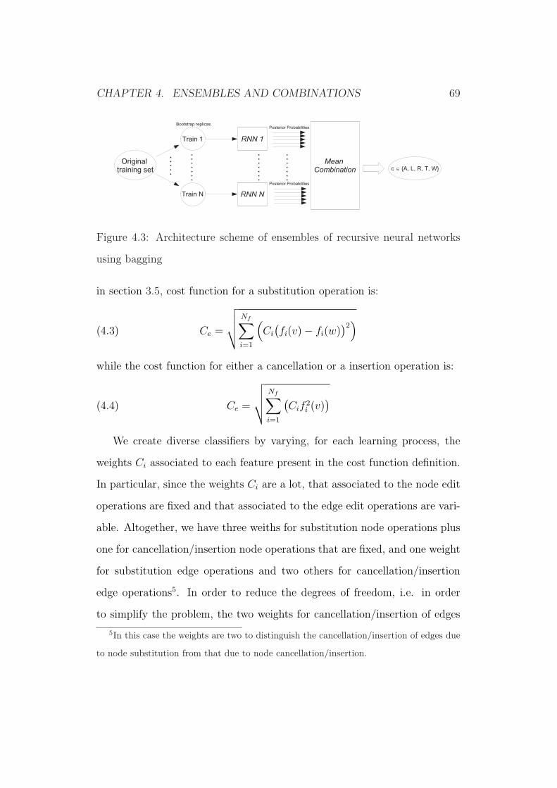
CHAPTER 4. ENSEMBLES AND COMBINATIONS 69
Figure 4.3: Architecture scheme of ensembles of recursive neural networks
using bagging
in section 3.5, cost function for a substitution operation is:
(4.3) Ce =
√√√√Nf∑i=1
(Ci
(fi(v)− fi(w)
)2)
while the cost function for either a cancellation or a insertion operation is:
(4.4) Ce =
√√√√Nf∑i=1
(Cif 2
i (v))
We create diverse classifiers by varying, for each learning process, the
weights Ci associated to each feature present in the cost function definition.
In particular, since the weights Ci are a lot, that associated to the node edit
operations are fixed and that associated to the edge edit operations are vari-
able. Altogether, we have three weiths for substitution node operations plus
one for cancellation/insertion node operations that are fixed, and one weight
for substitution edge operations and two others for cancellation/insertion
edge operations5. In order to reduce the degrees of freedom, i.e. in order
to simplify the problem, the two weights for cancellation/insertion of edges
5In this case the weights are two to distinguish the cancellation/insertion of edges due
to node substitution from that due to node cancellation/insertion.

CHAPTER 4. ENSEMBLES AND COMBINATIONS 70
are equal. Then, only two weights, that related to edge substitution opera-
tions and that related to edge cancellation/insertion operations, can vary to
generate different base classifiers.
The architecture of the combination system is similar to bagging with
RNNs one. Combination is still performed by mean rule. Figure 4.4 shows
this architecture.
Figure 4.4: Architecture scheme of ensembles of structural K nearest neigh-
bors, generated by varying internal parameters concerning edit distance def-
inition.

Chapter 5
Experimental Investigation
5.1 The data set
The NIST-4 database [Watson 1992], created by the National Institute of
Standard and Technology, is a reference data set widely used for assessing
and comparing fingerprint classification algorithms. It is made up of 4,000
ink-acquired fingerprint images, equally subdivided in five classes (A, L, R,
W, T). Each fingerprint was acquired two times. The first acquisition de-
notes the fingerprints from f0001 to f2000, the second acquisition denotes the
fingerprints from s0001 to s2000. We followed the experimental protocol gen-
erally used for such data set (see e.g. [Jain 1999 b, Yao 2003, Senior 2001]).
The first 1,800 fingerprints (f0001 through f900 and s0001 through s900) were
used for classifier training. The next 200 fingerprints were used as validation
set, necessary to perform early stopping of the neural classifiers (RNN and
MLP) during the learning phase, and the last 2,000 fingerprints as test set.
Seven hundred fingerprint images of NIST4 data set are labelled with two
classes instead of only one (”cross-referenced” fingerprints), as they could
71

CHAPTER 5. EXPERIMENTAL INVESTIGATION 72
not be reliably assigned to a unique class even by human experts. Table 5.1
shows the distribution of the classes in the NIST-4 data set. Rows indicate
the first class label, columns indicate the second class label. As an example,
the 29,7% of T class fingerprints are ”cross-referenced” with the R class. It
means that the 29.7% of T class fingerprints are labelled as ”TR”, class R be-
ing the second label for such fingerprints. Values along the diagonal indicate
the percentages of fingerprint images labelled with only one class. Typically
[Maltoni 2003], cross-referenced fingerprints are considered correctly classi-
fied if the classifier assigns them to one of the two classes. Table 5.1 points
out that an intrinsic confusion degree characterises the NIST-4 data set. In
A L R T W
A 95.0 0.0 0.3 4.7 0.0
L 0.0 94.5 0.0 5.2 0.3
R 0.0 0.0 93.3 6.2 0.5
T 18.8 20.7 29.7 30.8 0.0
W 0.0 0.3 0.7 0.0 99.0
Table 5.1: Distribution of the class labels in the NIST-4 Database. Rows
indicate the first class label, columns indicate the second class label.
order to use the FingerCode statistical representation [Jain 1999 b], we had
to disregard sixty-three fingerprint images due to the impossibility to find the
”core” point for such poor quality images. It should be noted that Jain et al.
also disregarded such fingerprint images in their experiments [Jain 1999 b].
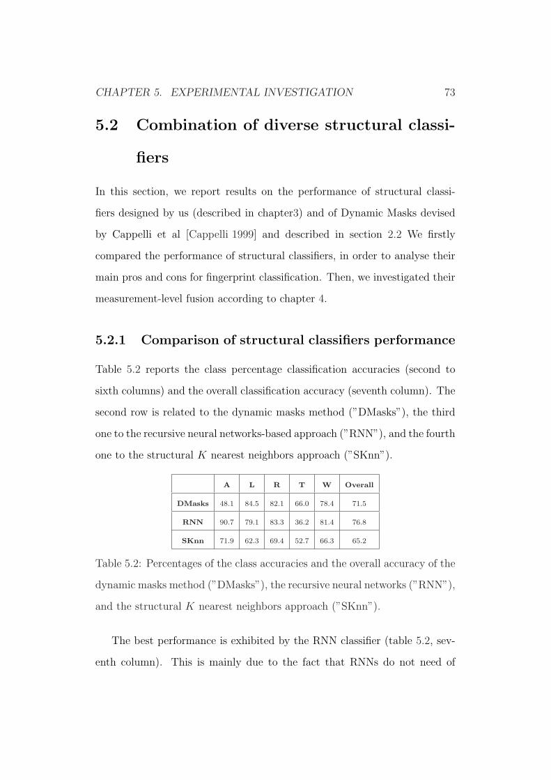
CHAPTER 5. EXPERIMENTAL INVESTIGATION 73
5.2 Combination of diverse structural classi-
fiers
In this section, we report results on the performance of structural classi-
fiers designed by us (described in chapter3) and of Dynamic Masks devised
by Cappelli et al [Cappelli 1999] and described in section 2.2 We firstly
compared the performance of structural classifiers, in order to analyse their
main pros and cons for fingerprint classification. Then, we investigated their
measurement-level fusion according to chapter 4.
5.2.1 Comparison of structural classifiers performance
Table 5.2 reports the class percentage classification accuracies (second to
sixth columns) and the overall classification accuracy (seventh column). The
second row is related to the dynamic masks method (”DMasks”), the third
one to the recursive neural networks-based approach (”RNN”), and the fourth
one to the structural K nearest neighbors approach (”SKnn”).
A L R T W Overall
DMasks 48.1 84.5 82.1 66.0 78.4 71.5
RNN 90.7 79.1 83.3 36.2 81.4 76.8
SKnn 71.9 62.3 69.4 52.7 66.3 65.2
Table 5.2: Percentages of the class accuracies and the overall accuracy of the
dynamic masks method (”DMasks”), the recursive neural networks (”RNN”),
and the structural K nearest neighbors approach (”SKnn”).
The best performance is exhibited by the RNN classifier (table 5.2, sev-
enth column). This is mainly due to the fact that RNNs do not need of
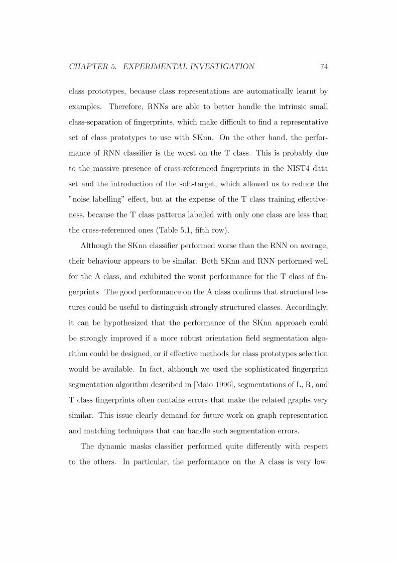
CHAPTER 5. EXPERIMENTAL INVESTIGATION 74
class prototypes, because class representations are automatically learnt by
examples. Therefore, RNNs are able to better handle the intrinsic small
class-separation of fingerprints, which make difficult to find a representative
set of class prototypes to use with SKnn. On the other hand, the perfor-
mance of RNN classifier is the worst on the T class. This is probably due
to the massive presence of cross-referenced fingerprints in the NIST4 data
set and the introduction of the soft-target, which allowed us to reduce the
”noise labelling” effect, but at the expense of the T class training effective-
ness, because the T class patterns labelled with only one class are less than
the cross-referenced ones (Table 5.1, fifth row).
Although the SKnn classifier performed worse than the RNN on average,
their behaviour appears to be similar. Both SKnn and RNN performed well
for the A class, and exhibited the worst performance for the T class of fin-
gerprints. The good performance on the A class confirms that structural fea-
tures could be useful to distinguish strongly structured classes. Accordingly,
it can be hypothesized that the performance of the SKnn approach could
be strongly improved if a more robust orientation field segmentation algo-
rithm could be designed, or if effective methods for class prototypes selection
would be available. In fact, although we used the sophisticated fingerprint
segmentation algorithm described in [Maio 1996], segmentations of L, R, and
T class fingerprints often contains errors that make the related graphs very
similar. This issue clearly demand for future work on graph representation
and matching techniques that can handle such segmentation errors.
The dynamic masks classifier performed quite differently with respect
to the others. In particular, the performance on the A class is very low.

CHAPTER 5. EXPERIMENTAL INVESTIGATION 75
In our opinion, such a low performance can be explained with the absence
of singularity points in the A class, which make quite difficult to design an
appropriate dynamic mask for that class. With regard to this issue, it should
be noted that the performance on the other classes, which exhibit at least
two singularities, is definitely higher.
5.2.2 Decision-level fusion of structural classifiers
First of all, the complementarity among the investigated structural classifiers
was investigated using the so called ”oracle”, that is, the ”ideal” combiner
able to select the classifier, if any, that correctly classifies the input pattern. It
should be noted that the oracle accuracy is usually a very optimistic estimate
of the performance achievable with classifier fusion rules. This is due to the
fact that the oracle give an estimation of the intersection degree among the
sets of misclassified patterns of the individual classifiers, without taking into
account the values of posterior probabilities output by them. In order to
overcome this limitation, we coupled the oracle results with the analysis of the
correlation coefficient among the outputs of each couple of the investigated
classifiers.
The performance of the oracle is shown in table 5.3.
The first column shows the ”fused” classifiers (the percentage accuracy
of the best individual classifier is reported in brackets), the second column
shows the performance of the related oracle. Table 5.3 points out that dy-
namic masks and the other structural classifiers exhibit a certain comple-
mentarity degree (second and third rows). It is also worth noting that the
highest classification rate can be potentially achieved by combining all three

CHAPTER 5. EXPERIMENTAL INVESTIGATION 76
FUSION of Oracle
DMasks-RNN (76.8) 91.1
DMasks-SKnn (71.5) 89.2
RNN-SKnn (76.8) 86.1
DMasks-RNN-SKnn (76.8) 94.1
Table 5.3: Performance of the oracle. Accuracy of the best classifier in each
combination is reported in brackets
investigated structural classifiers. This means that each classifier can sig-
nificantly contribute to the performance improvement. However, Table 5.4
shows that the correlation coefficient among their outputs per class is aver-
agely high, except for the couple RNN-DMasks and SKnn-DMasks on A and
T classes. These values could be expected because all methods are aimed to
describe the same data, i.e. the orientation field segmentation, and also they
use similar structural representations. Accordingly, it could be difficult to
exploiting the complementarity among these classifiers.
Class A Class L Class R Class T Class W
SKnn+DMasks 0.35 0.55 0.58 0.24 0.59
SKnn+RNN 0.81 0.59 0.66 0.46 0.63
DMasks+RNN 0.40 0.67 0.69 0.40 0.70
Table 5.4: Correlation coefficient computed among the individual classifiers.
For each classifiers pair, the correlation among class posterior probabilities
vectors of a test pattern is determined. Then, the mean for class is calculated.
Table 5.5 shows the performance of individual classifiers and their related
decision-level fusion with different combination rules.
The best performance is achieved by the fusion rules based on the KNN

CHAPTER 5. EXPERIMENTAL INVESTIGATION 77
FUSION of Mean Product KNN
DMasks-RNN (76.8) 80.6 79.2 81.7
DMasks-SKnn (71.5) 79.1 77.8 79.8
RNN-SKnn (76.8) 76.1 76.7 76.6
DMasks-RNN-SKnn (76.8) 82.4 82.2 83.6
Table 5.5: Percentage accuracy of the measurement-level fusion of the inves-
tigated structural classifiers by the mean rule, the product rule, multi-layer
perceptron (MLP) and K-nearest neighbour (KNN). The overall accuracy of
the best individual classifier is reported in brackets in the first column
when all the three structural classifiers are combined. But the simple mean
rule also gives a good performance (table 5.5, fifth row). This result points
out that the contribution of structural K nearest neighbors classifier is dif-
ficult to exploit, probably because of the low performance of this approach.
On the other hand, reported results points out the high complementarity
between the dynamic masks and RNN classifiers. The improvement of the
classification performance is about 7% and, according to the oracle results,
there is still room for further improvements (table 5.3, tab:structFus, fifth
row).

CHAPTER 5. EXPERIMENTAL INVESTIGATION 78
5.3 Comparison and combinations between
structural and statistical classifiers
5.3.1 Comparison among statistical and structural ap-
proaches
Table 5.6 reports the accuracy on the test set of the statistical classifier men-
tioned in Section 2.1, that is, the multi-layer perceptron using FingerCodes.
First of all, Table 5.6 shows that the overall accuracy of the statistical classi-
fier is higher than the one of any structural classifiers and their combination.
However, it is evident from tables 5.2 and 5.6 that, for the A class, the struc-
tural classifiers perform definitely better than the statistical one (except for
the dynamic masks method).
Class A Class L Class R Class T Class W Overall
Statistical classifier 80.5 91.8 89.5 79.1 89.4 86.0
Table 5.6: Percentage class accuracies and overall accuracy of multi-layer
perceptron trained with FingerCodes on NIST-4 test set
In order to investigate the advantages of structural approaches for dis-
criminating classes with a clear structure, for which standard statistical clas-
sifiers often perform not well, we analysed in detail the confusion degree
between the A and T classes. Table 5.7 shows the confusion degree between
the A and T classes (i.e., the percentage of fingerprints of the A class misclas-
sified as T class fingerprints) of the individual structural classifiers, their best
fusion, and the statistical classifier. It should be noted that the confusion
among such classes is a well-known issue for the state-of-the-art statistical
CHAPTER 5. EXPERIMENTAL INVESTIGATION 79
classifiers. Table 5.7 shows that structural approaches can be useful to rec-
ognize strongly structured fingerprint classes, such as the A class. Even for
the dynamic masks and the SKnn classifiers, which do not outperform the
statistical classifier individually, Table 5.7 shows that their fusion definitely
improve the performance.
Classifiers A - T confusion degree
DMasks 19.8
RNN 2.7
SKnn 19.4
Best fusion DMasks-RNN 4.5
Best fusion DMasks-SKnn 5.0
Best fusion RNN-SKnn 2.9
Best fusion DMasks-RNN-SKnn 5.2
Statistical classifier 16.7
Table 5.7: Percentage of A-T classes confusion degree of the individual clas-
sifiers (masks, RNN, SKnn), their best fusion, and the statistical classifier.
The best fusion has been reported according to the best overall accuracy
showed in table 5.5
5.3.2 Fusion of statistical and structural approaches
Table 5.8 reports the overall accuracy obtained by using the oracle and the
product, mean and KNN fusion rules (third, fourth, fifth and sixth columns,
respectively). We also reported the correlation coefficient of the maximum
posterior probabilities output by each statistical-structural classifiers couple
in the second column. These values, coupled with the oracle performance,
points out the strong complementarity between structural and statistical

CHAPTER 5. EXPERIMENTAL INVESTIGATION 80
approaches. In particular, the overall accuracy of the oracle reaches a value
near to the 100.0% in the case of the fusion of all classifiers. The other
columns shows that this complementarity can be exploited by the fusion
rules.
Fusion of Corr. Coeff. Oracle Mean Product KNN
Statistical-DMasks 0.30 93.0 84.4 83.5 86.2
Statistical-RNN 0.26 94.0 87.6 87.8 88.5
Statistical-SKnn 0.23 93.1 86.7 87.0 88.6
Ststistical-RNN-SKnn - 95.5 86.0 87.5 89.0
Statistical-DMasks-SKnn - 96.1 86.8 85.8 88.0
Statistical-DMasks-RNN - 96.5 88.2 85.8 88.8
Statistical-DMasks-RNN-SKnn - 97.2 88.6 87.0 89.6
Table 5.8: Percentage accuracy on overall of the oracle and the investigated
fusion rules. The correlation coefficient of each statistical-structural classi-
fiers couple is reported in the second column.
In particular, the good results of mean and product rules, which are
simpler than the KNN one, can be explained with the help of Table 5.9.
This table reports the mean of the posterior probability of each class for the
investigated structural and statistical classifiers. It shows that the outputs
of the statistical classifier are averagely higher than those of the structural
approaches, except for the DMasks classifier. This means that it is very
difficult to change the decisions of the statistical classifier. On the other
hand, structural K nearest neighbors and rnn classifiers exhibit a lower value,
especially for those classes they are not effective (L, R, T classes). This
means that, in many cases, their decision could be ‘corrected’ by a classifier
which exhibit a ‘stronger’ behaviour, namely, the statistical one. The same

CHAPTER 5. EXPERIMENTAL INVESTIGATION 81
observation can be made for the A class, where SKnn and RNN outperform
the statistical classifier. Their posterior probabilities on this class exhibit
a value higher than that of the statistical one. Accordingly, many wrong
decisions of the statistical approach on this class could be recovered (i.e.,
can be turned on right decisions) by the fusion with structural ones. In fact,
as the fusion by K-nn metaclassifier shows, better performance are achieved
when statistical classifier is combined with RNN or SKnn classifier, in spite
of the low overall accuracy of the last one.
Class A Class L Class R Class T Class W
SKnn 0.78 0.54 0.60 0.23 0.57
RNN 0.73 0.61 0.65 0.27 0.78
DMasks 0.43 0.80 0.76 0.40 0.76
Statistical 0.69 0.85 0.82 0.60 0.87
Table 5.9: Mean of class posterior probabilities for each class, for individual
classifiers on the test set
Figure 5.1 shows the accuracy-rejection curves of the best classifiers and
fusion approaches we investigated. The rejection option makes sense when
a fingerprint cannot be classified without a large margin of uncertainty, so
increasing the probability of wrong classification, and, consequently, increas-
ing the identification time. In this case, it can be better: (i) to leave the
decision to a human expert, or (ii) to submit the fingerprint to a specialised
classification module, if any, or (iii) to associate the fingerprint to the couple
of most probable classes (and doing a search in the data base limited to such
classes). The use of the rejection option obviously increases the final identifi-
cation time (Section 1). Therefore, a good trade-off between the percentage

CHAPTER 5. EXPERIMENTAL INVESTIGATION 82
2 4 6 8 10 12 14 16 18 2076
78
80
82
84
86
88
90
92
94
Rejection %
Acc
urac
y %
Masks+RNN+GM+Stat (KNN)Masks+RNN+Stat (KNN)GM+Stat (KNN)StatRNN
(a)
2 4 6 8 10 12 14 16 18 2070
75
80
85
90
95
100
Rejection %
Acc
urac
y %
Masks+RNN+GM+Stat (KNN)Masks+RNN+Stat (KNN)GM+Stat (KNN)StatRNN
(b)
Figure 5.1: The accuracy-rejection curves of the best classifiers and their
best fusion algorithm. Graphic 5.1(a) shows the overall accuracy, whereas
graphic 5.1(b) shows the accuracy of A class.
of rejected fingerprints and the required classification accuracy is needed.
As the FBI requirements for the NIST data bases are 99% of classification
accuracy with 20% rejection rate [Maltoni 2003, Karu 1996, Senior 2001],
we investigated accuracy for rejection rates ranging from 2% to 20% in our
experiments.
We followed the Chow’s rule for rejecting the pattern [Chow 1970], that is,
its maximum posterior probability should exceed a certain rejection thresh-
old otherwise it is considered as ”‘rejected”’ or not classified. From Figure
5.1, it is evident that, by increasing the number of structural classifiers, it
is possible to gradually improve the performance and also to obtain a bet-
ter classification accuracy when the rejection rate increases, especially for
class A accuracy. This confirms that each classifier contributed to the per-

CHAPTER 5. EXPERIMENTAL INVESTIGATION 83
formance improvement significantly, and also impacts on the reliablity of the
classification system.
5.4 Bagging with recursive neural networks
In this section, results on the performance of ensemble of recursive neural
networks generated using bagging approach is reported. As shown in section
4.2, Bagging is a typical method used for generating a multiple classifier
system, automatically from the same kind of base classifier. The diversity
of individual classifiers in the combination system is due by generating N
different bootstrap replicas of the original training set. It is well known
([Breiman 1996] that the number of training replicas must be infinite, that
is, N must be enough great to be considered infinite. How much great should
be N , dipendes on the particular application and it is not simple to find
its value. A typical solution is to learn many individual classifiers and to
stop the addition of classifiers in the combination system when the so called
”plateau” is found in the graphic representing the behaviour of combination
accuracy with respect to the number of individual classifiers. In this case,
i.e. recursive neural networks as base classifiers for fingerprint classification
on NIST4 database, it is chosen N = 100. Then, in order to combine the
base classifier outputs, mean rule is used. Figure 5.2 shows the behaviour of
bagging accuracy with respect to the N values.
The curve displais that the plateau is reached when about 30 base classi-
fiers are combined and the accuracy is approximately 76.6%. Since the overall
accuracy of a single recursive neural network, learned without using bagging,
is 76.8%, it is worth noting that bagging doesn’t improve performance of a

CHAPTER 5. EXPERIMENTAL INVESTIGATION 84
0 20 40 60 80 10075
75.5
76
76.5
77
77.5
N
Acc
urac
y
Bagging AccuracySingle Accuracy
Figure 5.2: Behaviour of bagging accuracy on the test set of NIST4 database
with respect to N. Base classifiers are recursive neural networks.
single recursive neural network.
As one could to expect, accuracy of base classifiers is a little worst with
respect to that of a single RNN; this fact is due to the instability intro-
duced by bootstrap technique. As the figure shows, the combination of base
classifiers improve with respect to them. In conclusion, seems that bagging
doesn’t work better than the single recursive neural network for fingerprint
classification.
5.5 Ensembles of structural K-nn
In this section, we report performance results of Ensembles of graph matchers,
where graph matchers are structural K nearest neighbors described in section
4.2.
As the computational complexity is too much and the learning process of
each individual classifier in the combination system is very time consuming,
CHAPTER 5. EXPERIMENTAL INVESTIGATION 85
it is not feasible to experiment it with all NIST4 dataset we used for the
other multiple classifier system, as described in sections 5.2 and 5.3.
Only one individual classifier is learned on all NIST4 dataset and its per-
formance are shown in table 5.2, fourth row. The overall accuracy reported
in this table is 65.2% and the classes accuracy is similar to that of recursive
neural network, i.e. the A class accuracy is very high with respect to the
overall accuracy, while other classes don’t achieve good performance, mostly
the T class. In our opinion, this similar behaviour is due to the fact that the
same image representation (i.e. the orientation field) and the same features
are used for both approaches.
In order to demonstrate the effectiveness of this method, aimed to create
ensembles of graph matchers in spite of computational difficulties, a reduced
set of 200 elements for the training set and other 200 elements for the test
set is extracted to NIST4 database; in order to respect the prior probabilities
of each class, patterns are randomly selected for the original dataset, that is,
the prior probabilities are all the same for each class with respect to the first
label of each pattern.
Table 5.10 shows accuracies on the test set of individual classifiers, gen-
erated by varying cost function of edit distance in the structural K nearest
neighbors. Each row represents a classifier. First and second columns are
edit operation weights that characterize differences of each classifier. As said
in section 4.2, only weights of edge edit operations vary to generate diverse
classifiers.
It is worth noting that performance of individual classifiers are not so
different. But combination of some of these classifiers, as shown in table 5.11,

CHAPTER 5. EXPERIMENTAL INVESTIGATION 86
C1 C2 Overall accuracy
15 5 62,00
3 1 58,50
10 1 57,50
15 3 57,50
15 1 57,50
20 2 56,00
30 3 58,00
17 4 62,50
16 2 58,50
17 1 58,00
10 5 60,50
15 5 62,00
10 8 62,00
10 1 61,50
5 1 62,50
Table 5.10: Accuracy of individual classifiers, generated by varying cost func-
tion of edit distance in the structural K nearest neighbors. Each row repre-
sents a classifier. First and second columns are edit operation weights that
characterize differences of each classifier.
improves performance of the best individual classifier. For the combination
phase, classifiers are selected on the basis of a validation set.
Each row is referred to a multiple classifier system. Each column, except
last one, indicates the overall accuracy of individual classifier, while last
column indicates the overall accuracy of multiple classifier system obtained
fusing the classifiers of the same row. It is worth noting that, by increasing
the number of individual classifiers, combination system doesn’t improve its

CHAPTER 5. EXPERIMENTAL INVESTIGATION 87
(a)
S1 S2 Fusione
60.5 61.5 65.5
60.5 62.5 67.0
62.0 60.5 64.5
57.5 60.5 63.5
(b)
S1 S2 S3 Fusione
62.5 60.5 62.5 67.0
62.5 60.5 58.5 65.5
57.5 57.5 57.5 62.0
57.5 60.5 62.5 63.5
(c)
S1 S2 S3 S4 S5 S6 Fusione
57.5 62.0 62.5 62.5 60.5 62.0 64.0
57.5 57.5 62.0 62.5 62.5 60.5 65.0
Table 5.11: Overall accuracies of ensembles of graph matchers fused by mean
rule. Combination architecture has of 3, 4 and 6 base classifiers, generated by
varying cost function of edit distance in the structural K nearest neighbors.
performance. In particular, the best combination is obtained both with the
two individual classifiers related to third row in the table 5.11(a) and with
three individual classifiers related to second row in the table 5.11(b).
Table 5.12 shows performance of individual classifiers (second and third
row) and related combination of the best fusion of ensembles of graph match-
ers (fourth row) in terms of class accuracies.
It is worth noting that the behaviour of individual classifiers is similar:
very high percentage of correct classified patterns for the A class and worst
performance for T and W classes. The A class classification improvement of

CHAPTER 5. EXPERIMENTAL INVESTIGATION 88
Class A Class L Class R Class T Class W Overall
Expert 1 70.45 73.81 57.89 58.06 51.11 62.50
Expert 2 72.09 69.05 48.72 58.06 53.33 60.50
Fusion 93.02 69.05 53.85 38.71 71.11 67.00
Table 5.12: Percentages of the class accuracies and the overall accuracy of
individual classifiers and related combination of the best fusion of ensembles
of graph matchers.
the combination is more than 20% with respect to the best A class accuracy
of single classifiers. Hence, A class accuracy becomes comparable with the A
class accuracy of diverse classifiers combination, namely, all structural and
statistical shown in section 5.3.2 (in particular, see figure 5.1(b)). Moreover,
also W class accuracy improves approximately of 20% with respect to W class
accuracies of single classifiers. Unfortunately, T class accuracy deteriorates
its performance.

Chapter 6
Conclusions
6.1 Conclusions on diverse classifiers fusion
In chapters 3 and 4 the structural approaches and its combination with the
statistical one were investigated. The aim of our study was:
1. to show the classes for which the structural approaches could be effec-
tive
2. to investigate the theoretical potentialities of structural-statistical fu-
sion
3. to investigate some fusion rules for exploiting such potentialities
We firstly trained and tested a recursive neural network for distinguishing
among fingerprints represented by a DPAG, a graph describing the fingerprint
structure. The proposed structural approach presented important modifica-
tions with respect to that proposed in previous works: we avoided the DPAG
generation dependence on the singularity points, which cannot be easily de-
tected in many computed fingerprint images; we reduced the noise labelling
89
CHAPTER 6. CONCLUSIONS 90
introduced by the ambiguous fingeprints by using a soft-target during the
RNN training.
Then, we trained and tested a structural K nearest neighbors for distin-
guishing among fingerprints represented by a relational graph describing the
fingerprint structure in a different way with respect to that of DPAG for re-
cursive neural networks. This proposed method is a tipical way for classifing
structural patterns, but it is the first time that it is applied to fingerprint
classification.
We combine these approaches and another relevant structural approach
reported in the literature, the dynamic masks approach, themselves and com-
pared their results with that of statistical classifier based on FingerCode. Ex-
perimental results appear to confirm that structural approaches can perform
better than statistical ones for the strongly structured fingerprint classes,
such as the A class. Moreover, their fusion can help in improving classifica-
tion performances and, in particular, to reduce the problem of A-T classes
confusion degree, which is a well- known issue for currently used statistical
classifiers. Although definitive conclusions cannot be drawn on the basis of
the above limited set of experiments, we believe that this work can contribute
to start the discussion about advantages and drawbacks of structural meth-
ods for fingerprint classification, and also to indicate some aspects worthy of
further investigations.
We combined the structural approaches results with those of a statisti-
cal approach based on the FingerCode. Reported results pointed out that
structural approaches can distinguish the A class much better than the sta-
tistical one. On the other hand, the structural approaches are not sufficient

CHAPTER 6. CONCLUSIONS 91
to achieve good classification performance on the other classes.
Then, we studied the complementarity among structural and statistical
approaches. The ”oracle” and the correlation coefficient of their outputs
used to this aim pointed out the strong complementarity among the above
approaches. In particular, the role of each approach to perfomance improve-
ment is quite different, being the structural aprroaches specialised on the A
class and the statistical one on the other classes.
Accordingly, we applied different fusion rules to exploit such complemen-
tarity: the fixed rules (non parametrical rules, so defining a simple fusion
architecture) and the so called meta-classification approach (a K nearest
neighbors, so defining a more complex fusion architecture). Reported re-
sults on fusion of structural and statistical approaches definitely showed the
improvement of the performance with respect to that of the best individ-
ual one. A sharp classification performance increase has been pointed out
both from fixed rules and meta-classifier. This result pointed out that such
complementarity exploitation does not often require very complex fusion ar-
chitectures. As an example, the mean rule exhibited a classification accuracy
superior than that presented by the KNN architecture on the W class; in
other cases, performance of fusion by KNN and the fixed rules were com-
parable. As expected, a powerful fusion rule, as the KNN metaclassifier,
has been able to better approximate the oracle behaviour, by working as a
”selector” among the structural classifiers and the statistical one for each
pattern class.
The complementarity esploitation of the decision-level structural-statistical
fusion has been confirmed by the recover rate analysis of all fusion rules. In

CHAPTER 6. CONCLUSIONS 92
particular, the investigated fusion rules exhibited a high capability of recov-
ering patterns wrongly classified by structural approaches. Many A class
pattern wrongly classified by the statistical approach have been recovered by
our fusion rules too.
Finally, as the accuracy-rejection trade-off is an important issue for a
real automatic fingerprint classification systems, reported accuracy-rejection
curves analysis based on the Chow’s theory pointed out that decision-level
fusion is more effective than the best individual approach (the statistical one
for the L-R-T-W classes, the structural ones for the A class) in improving the
overall performance when ambiguous fingerprint cannot be reliably classified.
Firstly, none of the few works investigating the structural fingerprint clas-
sification experimentally analysed the fingerprint classes for which a struc-
tural approach is useful. On the contrary, in this work, we clearly showed
the crucial role that the proposed structural approaches play in fingerprint
classification. Accordingly, the interest in structural fingerprint classifica-
tion should be renewed: other structural approaches could be analysed and
their fusion with other statistical approaches could be investigated to obtain
more general results than ours. Secondly, very few works about decision-level
structural-statistical fusion have been proposed so far. However, the high po-
tentiality of such fusion, which we showed in this work using different fusion
rules, should contribute to stimulate the interest around such challenging
topic. In particular, the design of decision-level fusion rules explicitly aimed
to exploit the structural-statistical complementarity is still an open issue.

CHAPTER 6. CONCLUSIONS 93
6.2 Conclusions on ensembles of graph match-
ers
Once designed the individual classifiers (recursive neural network and struc-
tural K nearest neighbors), they are adapted to generate ensembles, that is,
a lot of individual classifiers of the same type trained with some different
characteristic about internal parameters, input features or output features.
We trained and tested two kind of ensembles, the first regarding recur-
sive neural network with differences in input features, the latter regarding
structural K nearest neighbors with differences in internal parameters.
Ensembles of recursive neural networks, generated using bagging proce-
dure, have performance similar that obtained with a single recursive neural
network. Performance of the individual RNNs trained with bagging, are lower
than a single RNN trained without bagging perturbation. With respect to
base classifiers performance, ensembles improve their accuracy. Hence, al-
though the overall accuracy for fingerprint classification on NIST4 is not
better than the single classifier one, ensemble created by bagging works well,
like for statistical base classifiers.
Ensembles of structural K nearest neighbors are trained and tested on
a reduced dataset for computational complexity reasons. Base classifiers so
generated are weak classifiers and their performance are similar. Combina-
tion of some base classifiers outperforms with respect to the best individual
classifier. By increasing the number of individual classifiers, combination
system doesn’t improve its performance. It is probably due to the fact that
base classifiers have similar behaviour, hence few classifiers have a high com-

CHAPTER 6. CONCLUSIONS 94
plementarity with respect to the others. Regarding the single class accura-
cies, the behaviour of individual classifiers is similar: very high percentage
of correct classified patterns for the A class and worst performance for T
and W classes. The A class classification improvement of the combination is
more than 20% with respect to the best A class accuracy of single classifiers.
Moreover, also W class accuracy improves approximately of 20% with respect
to W class accuracies of single classifiers. Unfortunately, T class accuracy
deteriorates its performance.
Another time we found the most relevant result: structural classifiers, ei-
ther single or combined, are very usefull to distinguish the strong structured
classes, such as the A class for fingerprint classification. Like for diverse
structural-statistical combination, for ensembles of structural matchers too,
none of the few works investigating the structural fingerprint classification
experimentally analysed the fingerprint classes for which a structural ap-
proach is useful. On the contrary, in this work, we clearly showed the crucial
role that the proposed structural approaches play in fingerprint classifica-
tion. Accordingly, the interest in structural fingerprint classification should
be renewed: other approaches of ensembles of structural classifiers could be
analysed and investigated to obtain more general results than ours. Secondly,
very few works about ensembles of graph matchers have been proposed so
far, especially for fingerprint classification. However, the high potentiality
of such fusion, should contribute to stimulate the interest around such chal-
lenging topic. In particular, the design of other multiple classifiers systems
using graph-based approaches explicitly aimed to exploit the base classifiers
complementarity is still an open issue, which will be the subject of our future

CHAPTER 6. CONCLUSIONS 95
works.

Bibliography
[Jain 1999] A.A.V.V. ”Biometrics - Personal Identification in Networked So-
ciety”, edited by Anil Jain, Ruud Bolle e Sharath Pankanti - Kluwer
Academic Publisher, Boston/Dordrecht/London, 1999
[Wechsler 1997] Wechsler H., Phillips J.P., Bruce V., Folgeman Soulie F.,
Huang T.S.(Eds.), 1997 ”Face Recognition” - From theory to applica-
tions. Springer, ASI NATO Series, vol. 163
[Daugman 1993] Daugman J.G. 1993 ”High Confidence Visual Recognition
of Persons by a Test of Statistical Independence” IEEE TRansactions
on Pattern Analysis and Machine Intelligence, 15 (11) 1148-1161
[Furui 1997] S. Furui, ”Recent advances in speaker recognition”, ni Lectures
Notes in Computer Scienze 1206, Proceedings of Audio - and Video Bio-
metric Person Authentication AVBPA ’97, First International Confer-
ence, Crans-Montana, Switzerland, March 12-14 pp. 237-252, Springer-
Verlag, Berlin, 1997
[Prokoski 1992] F.J. Prokoski, R.B. Riedel, J.S. Coffin, ”Identification of in-
dividuals by means of facial thermography”, in Proceedings of The IEEE
1992 International Carnahan Conference on Security Technology: Crime
96

BIBLIOGRAPHY 97
Countermeasures, Atlanta, GA, USA 14-16 Oct., pp. 120-125, IEEE,
1992
[Hill 1978] R.B. Hill, ”Apparatus and method for identifying individuals
through their retinal vasculature patterns”, US Patent No. 4109237,
1978
[Zhang 2003] Zhang D., Kong W.K., You J., Wong M., 2003 ”Online Palm-
print Verification” IEEE Transactions on Pattern Recognition and Ma-
chine Intelligence 25 (9) 1041-1049
[Kumar 2003] Kumar A., Wong D.C.M., Shen H.C., Jain A.K., 2003 ”Per-
sonal Verification using Palmprint and Hand Geometry Biometric” Proc.
4th Int. Conf. on Audio- and Video- Based Person Authentication
AVBPA 2003, J. Kittler and M.S. Nixon Eds., Springer LNCS 2688,
pp. 668-678
[Herkel 2003] C. Herkel, H. Bunke, 2003 ”A set of novel features for writer
identification” Proc. of the 4th Int. Conf. on Audio- Based Person Au-
thentication AVBPA 2003, J. Kittler and M.S. Nixon Eds., Springer
LNCS 2688, pp. 679-687
[Kale 2003] A. Kale, N. Cuntoor, B. Yegnanarayana, A.N. Rajagopalan, R.
Chellappa, 2003 ”Gait analysis for human identification” Proc. of the
4th Int. Conf. on Audio- Based Person Authentication AVBPA 2003, J.
Kittler and M.S. Nixon Eds., Springer LNCS 2688, pp. 706-714

BIBLIOGRAPHY 98
[Mansfield 2002] A.J. Mansfield, J. Wayman, 2002 ”Best practices in testing
and reporting performance of biometric device” NLP Report CMSC
14/02
[Maltoni 2003] D. Maltoni, D. Maio, A.K. Jain, and S. Prabhakar, Handbook
of Fingerprint Recognition, Springer Verlag, 2003
[Henry 1900] E.R. Henry, Classification and Uses of Fingerprints, Routledge,
London, 1900
[Pankanti 2002] S. Pankanti, S. Prabhakar, A.K. Jain, 2002 ”On the indi-
viduality of fingerprints” IEEE Transactions on Pattern and Machine
Intelligence, 24 (8) 1010-1025
[Bolle 2002] R.M. Bolle, J.H. Connell, N.K. Ratha, 2002 ”Biometric perils
and patches” Pattern Recognition, 35 (12) 2727-2738
[Karu 1996] K. Karu and A.K. Jain, Fingerprint Classification, Pattern
Recognition, 29 (3) 389-404, 1996
[Lee 1994] H.C. Lee, R.E. Gaensslen (eds.) ”Advances in fingerprint technol-
ogy” CRC Press, 1994
[Ghong 1997] M. Chong et al., ” Geometric Framework for Fingerprint Image
Classification”, Pattern Recognition, vol. 30, no. 9, pp. 1475-1488, 1997
[Duda 2001] R. Duda, P. Hart, and D. Stork, Pattern Classification - Second
Edition, John Wiley & Sons, 2001
BIBLIOGRAPHY 99
[Candela 1995] G.T. Candela, P.J. Grother, C.I. Watson, R.A. Wilkinson,
and C.L. Wilson, PCASYS - A Pattern-Level Classification Automation
System for Fingerprints, NIST tech. Report NISTIR 5647, 1995
[Jain 1999 b] A. K. Jain, S. Prabhakar, L. Hong, ”A Multichannel Approach
to Fingerprintf Classification”, IEEE Transactions on Pattern Analysis
and Machine Intelligence, vol. 21, no. 4, pp.348-358, 1999
[Cappelli 1999] R. Cappelli, D. Maio, and D. Maltoni, Fingerprint classifi-
cation based on Multi-space KL, Proc. AutoID’99, Summit, NI, pp.117-
120, 1999
[Nagaty 2001] K.A. Nagaty, Fingerprint classification using Artificial Neu-
ral Networks: a combined structural and statistical approach, Neural
Networks, 14 (9) 1293-1305, 2001
[Yao 2003] Y. Yao, G.L. Marcialis, M. Pontil, P. Frasconi, and F. Roli, Com-
bining Flat and Structural Representations for Fingerprint Classification
with Recursive Neural Networks and Support Vector Machines, Pattern
Recognition, 36 (2) 397-406, 2003
[Moayer 1975] B. Moayer and K.S. Fu, A syntactic approach to fingerprint
pattern recognition, Pattern Recognition, 7, 1-23, 1975
[Rao 1980] K. Rao and K. Balck, Type Classification of Fingerprints: a Syn-
tactic Approach, IEEE Transactions on Pattern Analysis and Machine
Intelligence, 2 (3) 223-231, 1980

BIBLIOGRAPHY 100
[Lumini 1999] A. Lumini, D. Maio, and D. Maltoni, Inexact graph matching
for Fingerprint Classification, Machine Graphics and Vision, 8 (2) 241-
248, 1999
[Cappelli 1999 b] R. Cappelli, A. Lumini, D. Maio, and D. Maltoni, Fin-
gerprint Classification by Directional Image Partitioning, IEEE Trans-
actions on Pattern Analysis and Machine Intelligence, 21 (5) 402-421,
1999
[Neuhause 2005] M. Neuhaus and H. Bunke, A Graph Matching Based Ap-
proach to Fingerprint Classification Using Directional Variance, Proc. of
5th Int. Conf. on Audio- and Video-Based Biometric Person Authentica-
tion AVBPA’05, T. Kanade, A.K. Jain, N. Ratha Eds., Springer LNCS
3546, pp. 191-200, 2005.
[Neuhause 2005 b] M. Neuhaus and H. Bunke, Graph-Based Multiple Clas-
sifier System - A Data Levels Fusion Approach, Proc. of 13-th Int. Conf.
on Image Analysis and Processing ICIAP’05, F. Roli and S. Vitulano
Eds., Springer LNCS 3617, pp. 479-486, 2005.
[Senior 2001] A. Senior, A Combination Fingerprint Classifier, IEEE Trans-
actions on Pattern Analysis and Machine Intelligence, 23 (10) 1165-1174,
2001
[Cappelli 2002] R. Cappelli, D. Maio, and D. Maltoni, A Multi-Classifier Ap-
proach to Fingerprint Classification, Pattern Analysis and Applications,
5 (2) 136-144, 2002
BIBLIOGRAPHY 101
[Marcialis 2003] G.L. Marcialis, F. Roli, and A. Serrau, Fusion of Statistical
and Structural Fingerprint Classifiers, Proc. of 4th Int. Conf. on Audio-
and Video-Based Person Authentication AVBPA’03, (June, 9-11, 2003,
Guildford, U.K.), J. Kittler and M.S. Nixon Eds., Springer LNCS 2688,
pp. 310-317, 2003
[Serrau 2005] Serrau, A., Marcialis, G., Bunke, H., Roli, F.: An experimen-
tal comparison of fingerprint classification methods using graphs. In:
Proc. 5th Int. Workshop on Graph-based Representations in Pattern
Recognition. (2005)
[Maio 1996] D. Maio, D. Maltoni, A Structural Approach to Fingerprint
Classification, Proc. 13th ICPR, Vienna, pp. 578-585, 1996
[Windeatt 2003] T. Windeatt and F. Roli (Eds.), Multiple Classifier Sys-
tems, LNCS 2709, Springer Verlag, 2003
[Frasconi 1998] P. Frasconi, M. Gori, and A. Sperduti, A General Frame-
work for Adaptive Processing of Data Structures, IEEE Transactions on
Neural Networks, 9 (5) 768-786, 1998
[Yao 2001] Y. Yao, G.L. Marcialis, M. Pontil, P. Frasconi, and F. Roli, A New
Machine Learning Approach to Fingerprint Classification, Proc. of 7th
Congress of the Italian Association for Artificial Intelligence AIIA’01
(Bari, Italy, September 2001), F. Esposito Ed., Springer LNAI 2175,
pp.57-63, 2001

BIBLIOGRAPHY 102
[Sperduti 1997] A. Sperduti and A. Starita, Supervised neural networks for
the classification of structures, IEEE Transactions on Neural Networks
8 (3) 714-735, 1997
[Pollack 1990] J.B. Pollack ”REcursive distributed representations” Artifi-
cial Intelligence 46 (1-2) 77-106, 1990
[Plate 1995] T.A. Plate ”Holografic reduced representation” IEEE Transac-
tions on Neural Networks 6(3) 623-641, 1995
[Goller 1996] C. Goller and A. Kuchler, Learning task-dependent distributed
structure-representations by backpropagation through structure, in:
IEEE International Conference on Neural Networks, 347-352, 1996
[Frasconi 2001] P. Frasconi, M. Gori, and A. Sperduti, Special Section on
connectionist models for learning in structured domains, IEEE Trans-
actions on Knowledge and Data Engineering, 13 (2), 2001
[Bishop 1995] C.M. Bishop, Neural Networks for Pattern Recognition, Ox-
ford University Press, 1995
[Marcialis 2001] G.L. Marcialis, F. Roli, and P. Frasconi, Fingerprint Classi-
fication by Combination of Flat and Structural Approaches, Proc. of 3rd
International Conference on Audio- and Video- Based Biometric Person
Authentication AVBPA’01 (Halmstad, Sweden, 3-5 June 2001), J. Bigun
and F. Smeraldi Eds, Springer LNCS 2091, pp. 241-246, 2001
[Breiman 1996] Breiman, L.: Bagging predictors. Machine Learning 24
(1996) 123140

BIBLIOGRAPHY 103
[Ho 1998] T. K. Ho, The Random Subspace Method for Constructing Deci-
sion Forests, IEEE Transactions on Pattern Analysis and Machine In-
telligence, Vol. 20, 8, pp. 832-844, August 1998.
[Schenker 2004] A. Schenker, H. Bunke, M. Last, A. Kandel, ”Building
graph-based classifier ensembles by random node selection”, Proc. of
5th International Conference on Multiple Classifier System MCS’04
(Cagliari, Italy, June 2004), F. Roli, J Kittler, T. Windeatt Eds, Springer
LNCS 3077, pp. 214-222, 2004.
[Skurichina 2000] M. Skurichina, S. Raudys, and R.P.W. Duin, K- Nearest
Neighbors Directed Noise Injection in Multilayer Perceptron Training,
IEEE Transactions on Neural Networks, vol. 11, no. 2, 2000, 504-511
[Bunke 1983] H. Bunke and G. Allermann, Inexact Graph Matching for
Structural Pattern Recognition, Pattern Recognition Letters, 1 245-253,
1983.
[Watson 1992] C.I. Watson and C.L. Wilson, NIST Special Database 4, Fin-
gerprint Database, U.S. National Institute of Standard and Technology,
1992.
[Chow 1970] C.K. Chow, On optimum recognition error and reject tradeoff,
IEEE Transactions on Information Theory, 16:41-46, 1970.
[Roli 2002] F. Roli, F. Kittler, 2002. Multiple Classifier System. Springer-
Verlag, Lecture Notes in Computer Science, Vol. 2364.

BIBLIOGRAPHY 104
[Kittler 1998] J. Kittler, M. Hatef, R.P.W. Duin, J. Matas, 1998. On Com-
bining Classifiers. IEEE Transactions on Pattern Analysis and Machine
Intelligence, 20 (3) 226-239.
[Giacinto 1997] G. Giacinto, F. Roli, 1997. Ensembles of Neural Networks
for Soft Classification of Remote Sensing Images. European Symposium
on Intelligent Technologies, 20-21 March, Bari, Italy, pp.166-170