Embed Size (px)
Citation preview
Guidance Notes on Structural Analysis of Self-Elevating Units
GUIDANCE NOTES ON
STRUCTURAL ANALYSIS OF SELF-ELEVATING UNITS
APRIL 2016
American Bureau of Shipping Incorporated by Act of Legislature of the State of New York 1862
Copyright 2016 American Bureau of Shipping ABS Plaza 16855 Northchase Drive Houston, TX 77060 USA
ii ABS GUIDANCE NOTES ON STRUCTURAL ANALYSIS OF SELF-ELEVATING UNITS . 2016
F o r e w o r d
Foreword The guidance contained herein should be used in conjunction with the ABS Rules for Building and Classing Mobile Offshore Drilling Units for the purpose of ABS Classification of a Self-Elevating Unit. The guidance indicates acceptable practice in a typical case for types of designs that have been used successfully over many years of service. The guidance may need to be modified to meet the needs of a particular case, especially when a novel design or application is being assessed. The guidance should not be considered mandatory, and in no case is this guidance to be considered a substitute for the professional judgment of the designer or analyst. In case of any doubt about the application of this guidance ABS should be consulted.
A self-elevating unit is referred to herein as an “SEU”, and the ABS Rules for Building and Classing Mobile Offshore Drilling Units, are referred to as the “MODU Rules”.
These Guidance Notes become effective on the first day of the month of publication.
Users are advised to check periodically on the ABS website www.eagle.org to verify that this version of these Guidance Notes is the most current.
We welcome your feedback. Comments or suggestions can be sent electronically by email to [email protected].
Terms of Use
The information presented herein is intended solely to assist the reader in the methodologies and/or techniques discussed. These Guidance Notes do not and cannot replace the analysis and/or advice of a qualified professional. It is the responsibility of the reader to perform their own assessment and obtain professional advice. Information contained herein is considered to be pertinent at the time of publication, but may be invalidated as a result of subsequent legislations, regulations, standards, methods, and/or more updated information and the reader assumes full responsibility for compliance. This publication may not be copied or redistributed in part or in whole without prior written consent from ABS.
T a b l e o f C o n t e n t s
GUIDANCE NOTES ON
STRUCTURAL ANALYSIS OF SELF-ELEVATING UNITS CONTENTS SECTION 1 Introduction ............................................................................................ 1
1 Overview ............................................................................................. 1 3 General Requirements of Strength Analysis ....................................... 1 5 Information Required for Strength Analysis ........................................ 1
5.1 Unit’s Data ....................................................................................... 1 5.3 Gravity and Functional Load ............................................................ 2 5.5 Environmental Data ......................................................................... 2
7 Methods of Analysis ............................................................................ 8 7.1 Static Response .............................................................................. 8 7.3 Dynamic Response ......................................................................... 8
TABLE 1 Wind Pressure Height Coefficients ........................................... 3 FIGURE 1 Plot of Wind Force Height Coefficient vs. Height above
Design Water Surface ............................................................... 4 FIGURE 2 Current Velocity Profile ............................................................. 7 FIGURE 3 Water Depth .............................................................................. 7
SECTION 2 Loads ....................................................................................................... 9
1 Overview ............................................................................................. 9 3 Gravity and Functional Loads ............................................................. 9 5 Wind Load ......................................................................................... 10
5.1 Wind Load on Open Truss ............................................................. 10 5.3 Wind Load on Leg ......................................................................... 11 5.5 Dynamic Effects and Vortex Induced Vibration ............................. 11
7 Wave and Current Loads .................................................................. 11 7.1 Validity and Application of the Morison’s Equation ........................ 11 7.3 Hydrodynamic Coefficients ............................................................ 12 7.5 Wave Theories .............................................................................. 19 7.7 Asymmetry .................................................................................... 20 7.9 Stretching ...................................................................................... 20 7.11 Shielding ........................................................................................ 21 7.13 Wave Approach Angle ................................................................... 21 7.15 Breaking Wave and Slamming ...................................................... 21 7.17 Stepping Wave through Structures ................................................ 22
ABS GUIDANCE NOTES ON STRUCTURAL ANALYSIS OF SELF-ELEVATING UNITS . 2016 iii
9 Large Displacement Load (P-∆ Effect) .............................................. 22 9.1 Large Displacement Method .......................................................... 22 9.3 Geometric Stiffness Method .......................................................... 22
11 Dynamic Load (Inertial Effect)........................................................... 24 11.1 Magnitude of Inertial Load ............................................................. 24 11.3 Distribution of Inertial Load ............................................................ 24
13 Leg Inclination ................................................................................... 24 TABLE 1 P-∆ Effect Approaches ............................................................ 23 FIGURE 1 Non-cylindrical Chords ............................................................ 13 FIGURE 2A Drag Coefficient of Tubular Chord with Rack: Deterministic
Analysis ................................................................................... 14 FIGURE 2B Drag Coefficient of Triangular Chords: Deterministic
Analysis ................................................................................... 14 FIGURE 3 One Bay of Lattice Leg ........................................................... 17 FIGURE 4 Split-Tube Chord Section ........................................................ 17 FIGURE 5 Triangular Chord Section ........................................................ 18 FIGURE 6 Wave Theories Applicability Regions (After API RP2A) ......... 19 FIGURE 7 Wheeler Stretching of Wave ................................................... 21
SECTION 3 Structural Analysis Models ................................................................. 25
1 Overview ........................................................................................... 25 3 Structural Model ................................................................................ 25
3.1 Hierarchy of Models ....................................................................... 25 3.3 Hull Model ...................................................................................... 27 3.5 Leg Model ...................................................................................... 28 3.7 Leg-to-Hull Connection Model ....................................................... 30 3.9 Foundation Modeling ..................................................................... 36
TABLE 1 Applicability of Leg Models ..................................................... 25 TABLE 2 Applicability of Hull Models ..................................................... 25 TABLE 3 Applicability of Connection Models ......................................... 26 TABLE 4 Comparisons of Global Models ............................................... 26 FIGURE 1 Simplified Guide Modeling ...................................................... 33 FIGURE 2 Linearization of Guides ........................................................... 35 FIGURE 3 Eccentricity of Spudcan .......................................................... 37
SECTION 4 Structural Analyses .............................................................................. 38
1 Overview ........................................................................................... 38 1.1 Two-Step Procedure Analysis ....................................................... 38 1.3 Step 1 – Dynamic Analysis and Inertial Load Set .......................... 38 1.5 Step 2 – Quasi-static Analysis ....................................................... 39 1.7 Critical Storm Load Directions ....................................................... 40 1.9 Exception ....................................................................................... 40
iv ABS GUIDANCE NOTES ON STRUCTURAL ANALYSIS OF SELF-ELEVATING UNITS . 2016
3 Specification of Wave Parameters and Spudcan-Soil Stiffness ....... 41 3.1 Introduction .................................................................................... 41 3.3 Spectral Characterization of Wave Data for Dynamic Analysis ..... 42 3.5 Spudcan-Soil Rotational Stiffness (SC-S RS) ............................... 42
5 Dynamic Analysis Modeling .............................................................. 43 5.1 Introduction .................................................................................... 43 5.3 Stiffness Modeling ......................................................................... 43 5.5 Modeling the Mass ........................................................................ 45 5.7 Hydrodynamic Loading .................................................................. 45 5.9 Damping ........................................................................................ 45
7 Dynamic Response Analysis Methods ............................................. 46 7.1 General.......................................................................................... 46 7.3 Random Wave Dynamic Analysis in Time Domain ....................... 46 7.5 Other Dynamic Analysis Methods ................................................. 53
9 Dynamic Amplification Factor and Inertial Load Set ......................... 55 9.1 Introduction .................................................................................... 55 9.3 Inertial Load Set based on Random Wave Dynamic Analysis ....... 55 9.5 Inertial Load Set based on SDOF Approach ................................. 56 9.7 Inertial Load Set Applications ........................................................ 56
FIGURE 1 Flowchart of Two-step Procedure ........................................... 41 FIGURE 2 The Drag-Inertia Method Including DAF Scaling Factor ......... 50 FIGURE 3 Graphical Representation of DAF Scaling Factor, FDAF,
Applied in the Drag-Inertia Method ......................................... 51 SECTION 5 Commentary on Acceptance Criteria ................................................. 57
1 Introduction ....................................................................................... 57 3 Categories of Criteria ........................................................................ 57 5 Wave Crest Clearance and Air Gap ................................................. 57 7 Overturning Stability .......................................................................... 57 9 Structural Strength ............................................................................ 58
9.1 Yield Criteria .................................................................................. 58 9.3 Buckling Criteria ............................................................................ 59 9.5 Hybrid Members ............................................................................ 59 9.7 Punching Shear ............................................................................. 60 9.9 P-∆ Effect on Member Checking .................................................... 60
11 Fatigue of Structural Details.............................................................. 60 13 Strength of the Elevating Machinery ................................................. 60 15 Spudcan Check ................................................................................. 61
15.1 Preload Condition .......................................................................... 61 15.3 Normal Operating and Severe Storm Conditions .......................... 61
17 Other Checks .................................................................................... 61 FIGURE 1 Chords Section Stress Points ................................................. 60
ABS GUIDANCE NOTES ON STRUCTURAL ANALYSIS OF SELF-ELEVATING UNITS . 2016 v
APPENDIX 1 Equivalent Section Stiffness Properties of a Lattice Leg ................. 62 1 Introduction ....................................................................................... 62 3 Formula Approach ............................................................................ 62
3.1 Equivalent Shear Area of 2D Lattice Structures ............................ 62 3.3 Equivalent Section Stiffness Properties of 3D Lattice Legs ........... 63
TABLE 1 Equivalent Shear Area of 2D Lattice Structures ..................... 64 TABLE 2 Equivalent Moment of Inertia Properties of 3D Lattice
Legs ........................................................................................ 65 FIGURE 1 Shear Force System for X Bracing and its Equivalent
Beam ....................................................................................... 62 APPENDIX 2 Equivalent Leg-to-Hull Connection Stiffness Properties .................. 66
1 Introduction ....................................................................................... 66 3 Empirical Formula Approach ............................................................. 66
3.1 Horizontal Stiffness ........................................................................ 66 3.3 Vertical Stiffness ............................................................................ 66 3.5 Rotational Stiffness ........................................................................ 66
5 Unit Load Approach .......................................................................... 67 5.1 Unit Axial Load Case ..................................................................... 67 5.3 Unit Moment Case ......................................................................... 67 5.5 Unit Shear Load Case ................................................................... 67
APPENDIX 3 References ............................................................................................ 68
vi ABS GUIDANCE NOTES ON STRUCTURAL ANALYSIS OF SELF-ELEVATING UNITS . 2016
S e c t i o n 1 : I n t r o d u c t i o n
S E C T I O N 1 Introduction
1 Overview These Guidance Notes provide suggested practices that can be used in the structural analysis of a self-elevating unit (also referred to herein as an ‘SEU’ or a ‘unit’) in the elevated condition. The emphasis is on analyses that are used to assess the structural strength of the unit to resist yielding and buckling failure modes considering the static, and as needed the dynamic, responses of the unit in accordance with the ABS Rules for Building and Classing Mobile Offshore Drilling Units (MODU Rules). As an aid to users of the Rules, these Guidance Notes also provide explanations on the intent and background for some of the related criteria contained in the Rules.
3 General Requirements of Strength Analysis A unit’s modes of operation in an elevated condition should be investigated using anticipated loads, including gravity, functional and environmental loads. The Owner is to specify the environmental conditions for which the plans for the unit are to be approved. Owners or designers are to thoroughly investigate the environmental and loading conditions for each water depth considered in the Classification. It is the Owner’s responsibility to ensure that the unit is not exposed to conditions more severe than those for which it has been approved.
A unit with an ‘Unrestricted Classification’ is designed considering a minimum wind speed of 100 knots in the elevated severe storm condition, and 70 knots in the elevated normal drilling condition. The wave and other conditions that accompany these winds are to be as specified by the Owner. These other conditions, especially those related to waves and currents may not be the maximum values that are expected during the operational life of the unit. Accordingly other sets of environmental and other design parameters are typically specified by the Owner and are included in the scope of the unit’s Classification.
5 Information Required for Strength Analysis Sufficient information needs to be obtained to adequately perform the structural analysis on the unit.
5.1 Unit’s Data Basic information about the unit’s configuration is required for the analysis. These data are summarized below.
5.1.1 Structural Information Most of the structural information is obtained from relevant drawings and reports. These data can be categorized as:
• The primary sizes, scantlings and locations of structural members
• The detailed sections, connections and localized designs of structural members
• The material properties of structural members
• The characteristics of some machinery equipment that affect structural response
ABS GUIDANCE NOTES ON STRUCTURAL ANALYSIS OF SELF-ELEVATING UNITS . 2016 1
Section 1 Introduction
In particular, the properties of leg-to-hull connections are of great importance and need special attention:
• The basic configuration and arrangement of connections, which include pinions, chocks (if any), upper/lower guides, jacking case, shock pads (if any), etc.
• The stiffness and capacity of pinions and chocks (if any)
• The gap between leg chords and upper/lower guides
• The detailed structural configuration of jacking case
• The detailed structural configuration of upper/lower guides
5.1.2 Other Information Other data that are required for the SEU strength analysis include:
• Wind projected areas of the hull, deckhouses, derrick, drilling floor and leg in each direction
• The capacity and moving range of the cantilever
• The capacity of jacking system
5.3 Gravity and Functional Load The gravity loads include: steel weights, equipment and outfitting weights, the weights of liquid and solid variable quantities; and live loads. The gravity loads should be taken into account for the structural design and stability. The load effects due to operations such as drilling, work over and well servicing (rotary/hook loads and tensioner loads) should also be taken into account as functional loads.
For all modes of operation, the combinations of gravity and functional loads are specified by the Owner for the operations considered in the design. However, maximums (or minimums) of the combinations that produce the most unfavorable load effects on the unit’s strength or stability should be used in the design.
Total elevated load defined in 3-1-1/16 of the MODU Rules consists of the lightship weight excluding legs and spudcans, all shipboard and drilling equipment and associated piping, the liquid and solid variables and combined drilling (functional) load. The total elevated load is normally used to identify the capacity of an SEU in the elevated mode.
The following information needs to be collected:
• The magnitude and distribution of the lightship weight
• The magnitude and distribution of variable loads
• The magnitude and location of functional loads
• The magnitude and distribution of the total elevated load
• Extreme limits of center of gravity for the whole hull and the corresponding load magnitude
• Weight, center of gravity and buoyancy of the legs including non-structural parts.
5.5 Environmental Data Environmental loads contribute most of the horizontal forces acting on a unit, which are usually the controlling factors to determine the capacity of the unit. Below, the environmental data requirements as per 3-1-3 of MODU Rules are discussed. Each of the following environmental parameters that affect the loads acting on a jack-up unit is discussed:
• Wind
• Wave
• Current
• Water depth
2 ABS GUIDANCE NOTES ON STRUCTURAL ANALYSIS OF SELF-ELEVATING UNITS . 2016
Section 1 Introduction
• Airgap and wave clearance
• Geotechnical data
5.5.1 Wind The MODU Rules specify that for unrestricted offshore service, a unit should be designed for an operating wind velocity of at least 36 m/s (70 knots) and at least 51.5 m/s (100 knots) for a severe storm condition.
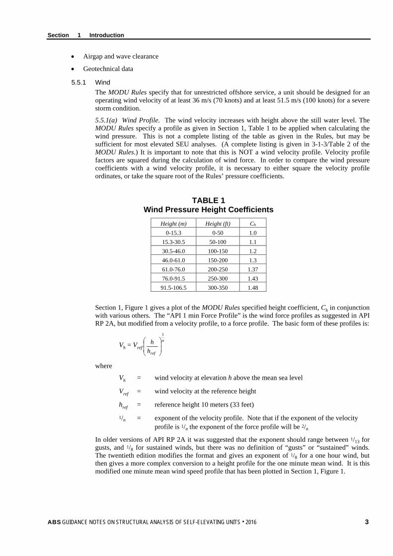
5.5.1(a) Wind Profile. The wind velocity increases with height above the still water level. The MODU Rules specify a profile as given in Section 1, Table 1 to be applied when calculating the wind pressure. This is not a complete listing of the table as given in the Rules, but may be sufficient for most elevated SEU analyses. (A complete listing is given in 3-1-3/Table 2 of the MODU Rules.) It is important to note that this is NOT a wind velocity profile. Velocity profile factors are squared during the calculation of wind force. In order to compare the wind pressure coefficients with a wind velocity profile, it is necessary to either square the velocity profile ordinates, or take the square root of the Rules’ pressure coefficients.
TABLE 1 Wind Pressure Height Coefficients
Height (m) Height (ft) Ch 0-15.3 0-50 1.0
15.3-30.5 50-100 1.1 30.5-46.0 100-150 1.2 46.0-61.0 150-200 1.3 61.0-76.0 200-250 1.37 76.0-91.5 250-300 1.43 91.5-106.5 300-350 1.48
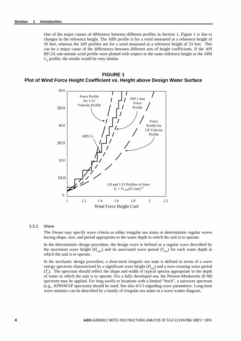
Section 1, Figure 1 gives a plot of the MODU Rules specified height coefficient, Ch in conjunction with various others. The “API 1 min Force Profile” is the wind force profiles as suggested in API RP 2A, but modified from a velocity profile, to a force profile. The basic form of these profiles is:
Vh = Vrefn
refhh
1
where
Vh = wind velocity at elevation h above the mean sea level
Vref = wind velocity at the reference height
href = reference height 10 meters (33 feet)
1/n = exponent of the velocity profile. Note that if the exponent of the velocity profile is 1/n the exponent of the force profile will be 2/n
In older versions of API RP 2A it was suggested that the exponent should range between 1/13 for gusts, and 1/8 for sustained winds, but there was no definition of “gusts” or “sustained” winds. The twentieth edition modifies the format and gives an exponent of 1/8 for a one hour wind, but then gives a more complex conversion to a height profile for the one minute mean wind. It is this modified one minute mean wind speed profile that has been plotted in Section 1, Figure 1.
ABS GUIDANCE NOTES ON STRUCTURAL ANALYSIS OF SELF-ELEVATING UNITS . 2016 3
Section 1 Introduction
One of the major causes of difference between different profiles in Section 1, Figure 1 is due to changes in the reference height. The ABS profile is for a wind measured at a reference height of 50 feet, whereas the API profiles are for a wind measured at a reference height of 33 feet. This can be a major cause of the differences between different sets of height coefficients. If the API RP-2A one-minute wind profile were plotted with respect to the same reference height as the ABS Ch profile, the results would be very similar.
FIGURE 1 Plot of Wind Force Height Coefficient vs. Height above Design Water Surface
1 1.2 1.4 1.6 1.8 2 2.20
10.0
30.0
20.0
40.0
50.0
60.0
ABS Ch
Force Profile for 1/12
Velocity Profile
Force Profile for
1/8 Velocity Profile
API 1 min Force Profile
1/8 and 1/12 Profiles of form:Vz = V1.0m(Z/1.0m)1/n
Wind Force Height Coef
5.5.2 Wave The Owner may specify wave criteria as either irregular sea states or deterministic regular waves having shape, size, and period appropriate to the water depth in which the unit is to operate.
In the deterministic design procedure, the design wave is defined as a regular wave described by the maximum wave height (Hmax) and its associated wave period (Tass) for each water depth in which the unit is to operate.
In the stochastic design procedure, a short-term irregular sea state is defined in terms of a wave energy spectrum characterized by a significant wave height (Hsrp) and a zero-crossing wave period (Tz). The spectrum should reflect the shape and width of typical spectra appropriate to the depth of water in which the unit is to operate. For a fully developed sea, the Pierson-Moskowitz (P-M) spectrum may be applied. For long swells or locations with a limited “fetch”, a narrower spectrum (e.g., JONSWAP spectrum) should be used. See also 4/3.3 regarding wave parameters. Long-term wave statistics can be described by a family of irregular sea states in a wave scatter diagram.
4 ABS GUIDANCE NOTES ON STRUCTURAL ANALYSIS OF SELF-ELEVATING UNITS . 2016
Section 1 Introduction
5.5.2(a) Design Wave Selection. The selected design wave should induce the most unfavorable response of the structure under consideration. Most SEU analyses for Classification are based on a deterministic wave approach, even when dynamics are being included, although appropriate spectral data can be used.
The wave (and current) conditions, which are to be combined with the Rule required minimum wind speeds, are those specified by the Owner. For other wave conditions specified by the Owner for inclusion in the scope of classification, they should be the maximum wave heights appropriate to the depths of water in which the unit is expected to operate.
Where dynamic effects are insignificant, the wave forces on an SEU are not too sensitive to the choice of wave period, except in unusual cases (e.g., where wave force cancellation occurs). It is therefore normally acceptable to use the maximum wave height with a single “Associated Wave Period”, as described below. Where dynamic effects are considered potentially significant, the choice of period can be critical, thus a range of wave periods associated with a range of wave heights are to be investigated.
At a certain wave period, the wave forces acting on an SEU will be significantly reduced due to force cancellation. The selected design wave should not be a wave that causes wave force cancellation. This occurs when there is a wave crest at one leg (or a set of legs) and a trough at another. For example, a unit with a leg spacing of 60 meters (200 feet) will experience cancellation in regular waves of approximately 8.8-second period. The length of an 8.8-second wave is 120 meters (400 feet) which is twice the leg spacing. The effect is more severe for four legged units than for three legged units. In the extreme case, the wave force on a four legged unit will be reduced to zero with perfect cancellation, whereas a three legged unit will effectively always have a different number of legs at the crest then at the trough. It is also possible to have wave force reinforcement at shorter wave periods, with wave crests at both sets of legs. Both reinforcement and cancellation can also occur at shorter periods due to harmonic effects. Under certain circumstances, the response to the component of the sea state close to resonance may be significantly reduced if the periods of resonance and cancellation happen to coincide.
5.5.2(b) Variations in Defining Wave Periods
i) Peak Period (Tp). Also known as the “Modal Period”, it is the wave period associated with the “peak” of the wave energy spectrum. It is normally longer than the period associated with the maximum wave.
ii) Mean Period (Tm). The Mean Period is the period corresponding to the centroid of the area enclosed under the wave spectrum. The mean period for a Pierson-Moskowitz (P-M) spectrum equals Tp/1.296.
iii) Mean Zero Crossing Period (Tz). The Mean Zero Crossing Period is the average time between the instances when the instantaneous water surface crosses the mean still water surface, moving in a specific direction (normally the up-crossing period). Normally 0.75Tp < Tz < 0.82Tp.
iv) Associated Period (Tass). The Associated Period is the period associated with the highest wave. Most of the other sea state wave periods are based on statistics for that sea state, but there is only one maximum wave in any given storm, so the associated period is the most probable period of the maximum wave. For this reason it is common to give a range of wave periods for Tass that are independent of Tp. One common range is to have
sasss HTH 2012 << , where Hs is the significant wave height in meters.
5.5.2(c) Dynamic Response. When an analysis for dynamic response due to waves, or waves with current, is being pursued, a spectral characterization of selected sea state is needed, refer to 4/3.3 for this topic.
ABS GUIDANCE NOTES ON STRUCTURAL ANALYSIS OF SELF-ELEVATING UNITS . 2016 5
Section 1 Introduction
5.5.3 Current The Owner is to specify the current velocity from water surface to seabed. For Classification, current is normally assumed to act collinearly with wind and wave.
When determining loads due to the simultaneous occurrence of wave and current using Morison’s equation, the current velocity is to be added vectorially to the wave particle velocity before the total force is computed. When diffraction methods are used for calculating wave force, the drag force due to current should be calculated in accordance with Section 3-1-3 of the MODU Rules and added vectorially to the calculated wave force.
The significance of current loads should not be underestimated, particularly in relatively benign environments. The effects of current are greatest on drag force dominated lattice leg units, but they can still be significant on large tubular legged units. On a drag dominant structure, the force is proportional to the square of the water particle velocity, so even a 10% increase in particle velocity due to current will cause a 20% increase in hydrodynamic load.
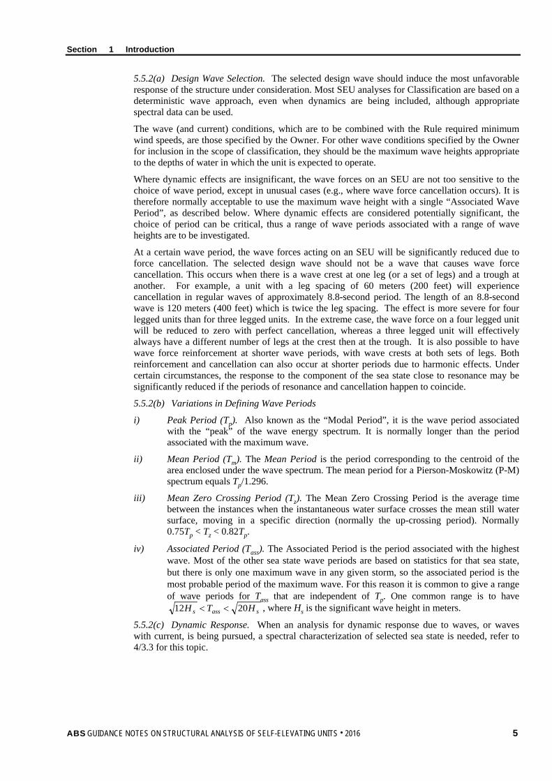
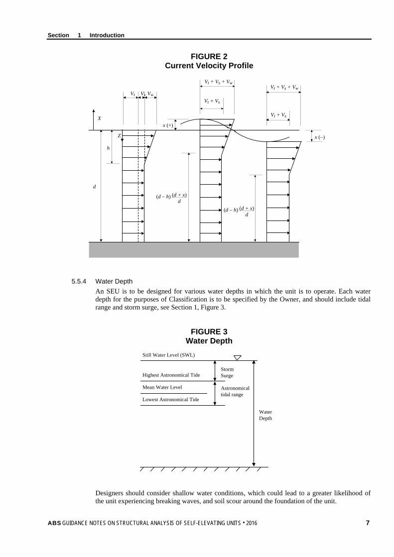
5.5.3(a) Current Associated with Waves. The current velocity is to include components due to tidal current, storm surge current and wind driven current. In lieu of a defensible alternative method, the recommended vertical distribution of current velocity in still water and its modification in the presence of waves, is as shown in Section 1, Figure 2 below, where:
Vc = Vt + Vs + Vw [(h − z)/h] for z ≤ h
Vc = Vt + Vs for z > h
where
Vc = current velocity, m/s (ft/s)
Vt = component of tidal current velocity in the direction of the wind, m/s (ft/s)
Vs = component of storm surge current, m (ft)
Vw = wind driven current velocity, m/s (ft/s)
h = reference depth for wind driven current, m (ft). (in the absence of other data, h may be taken as 5 m (16.4 ft).
z = distance below still water level under consideration, m (ft)
d = still water depth, m (ft)
In the presence of waves, the current velocity profile is to be modified, as shown in Section 1, Figure 2, such that the current velocity at the instantaneous free surface is a constant.
6 ABS GUIDANCE NOTES ON STRUCTURAL ANALYSIS OF SELF-ELEVATING UNITS . 2016
Section 1 Introduction
FIGURE 2 Current Velocity Profile
X
Vt Vs Vw
Vt + Vs + VwVt + Vs + Vw
Vt + Vs
Vt + Vs
x (+)
x (−)
(d + x)d
(d − h)
(d + x)d
(d − h)
d
h
Z
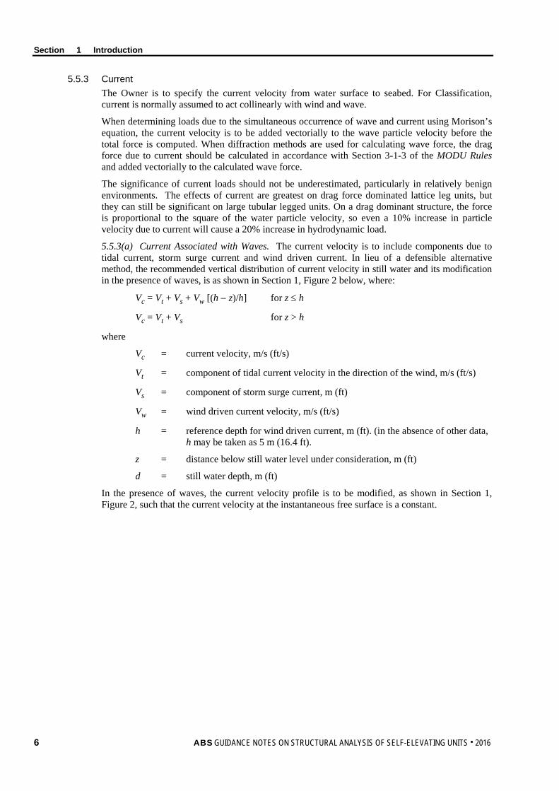
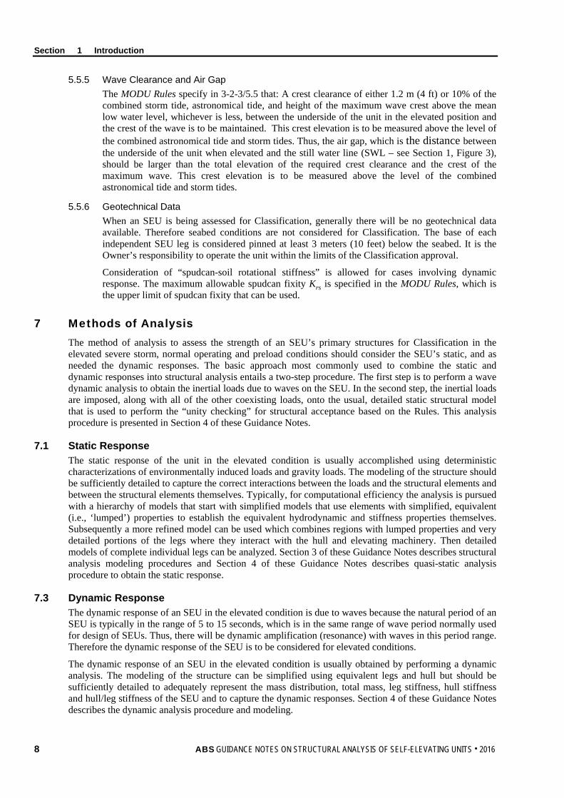
5.5.4 Water Depth An SEU is to be designed for various water depths in which the unit is to operate. Each water depth for the purposes of Classification is to be specified by the Owner, and should include tidal range and storm surge, see Section 1, Figure 3.
FIGURE 3 Water Depth
Still Water Level (SWL)
Highest Astronomical Tide
Mean Water Level
Lowest Astronomical Tide
Storm Surge
Astronomicaltidal range
WaterDepth
Designers should consider shallow water conditions, which could lead to a greater likelihood of the unit experiencing breaking waves, and soil scour around the foundation of the unit.
ABS GUIDANCE NOTES ON STRUCTURAL ANALYSIS OF SELF-ELEVATING UNITS . 2016 7
Section 1 Introduction
5.5.5 Wave Clearance and Air Gap The MODU Rules specify in 3-2-3/5.5 that: A crest clearance of either 1.2 m (4 ft) or 10% of the combined storm tide, astronomical tide, and height of the maximum wave crest above the mean low water level, whichever is less, between the underside of the unit in the elevated position and the crest of the wave is to be maintained. This crest elevation is to be measured above the level of the combined astronomical tide and storm tides. Thus, the air gap, which is the distance between the underside of the unit when elevated and the still water line (SWL – see Section 1, Figure 3), should be larger than the total elevation of the required crest clearance and the crest of the maximum wave. This crest elevation is to be measured above the level of the combined astronomical tide and storm tides.
5.5.6 Geotechnical Data When an SEU is being assessed for Classification, generally there will be no geotechnical data available. Therefore seabed conditions are not considered for Classification. The base of each independent SEU leg is considered pinned at least 3 meters (10 feet) below the seabed. It is the Owner’s responsibility to operate the unit within the limits of the Classification approval.
Consideration of “spudcan-soil rotational stiffness” is allowed for cases involving dynamic response. The maximum allowable spudcan fixity Krs is specified in the MODU Rules, which is the upper limit of spudcan fixity that can be used.
7 Methods of Analysis The method of analysis to assess the strength of an SEU’s primary structures for Classification in the elevated severe storm, normal operating and preload conditions should consider the SEU’s static, and as needed the dynamic responses. The basic approach most commonly used to combine the static and dynamic responses into structural analysis entails a two-step procedure. The first step is to perform a wave dynamic analysis to obtain the inertial loads due to waves on the SEU. In the second step, the inertial loads are imposed, along with all of the other coexisting loads, onto the usual, detailed static structural model that is used to perform the “unity checking” for structural acceptance based on the Rules. This analysis procedure is presented in Section 4 of these Guidance Notes.
7.1 Static Response The static response of the unit in the elevated condition is usually accomplished using deterministic characterizations of environmentally induced loads and gravity loads. The modeling of the structure should be sufficiently detailed to capture the correct interactions between the loads and the structural elements and between the structural elements themselves. Typically, for computational efficiency the analysis is pursued with a hierarchy of models that start with simplified models that use elements with simplified, equivalent (i.e., ‘lumped’) properties to establish the equivalent hydrodynamic and stiffness properties themselves. Subsequently a more refined model can be used which combines regions with lumped properties and very detailed portions of the legs where they interact with the hull and elevating machinery. Then detailed models of complete individual legs can be analyzed. Section 3 of these Guidance Notes describes structural analysis modeling procedures and Section 4 of these Guidance Notes describes quasi-static analysis procedure to obtain the static response.
7.3 Dynamic Response The dynamic response of an SEU in the elevated condition is due to waves because the natural period of an SEU is typically in the range of 5 to 15 seconds, which is in the same range of wave period normally used for design of SEUs. Thus, there will be dynamic amplification (resonance) with waves in this period range. Therefore the dynamic response of the SEU is to be considered for elevated conditions.
The dynamic response of an SEU in the elevated condition is usually obtained by performing a dynamic analysis. The modeling of the structure can be simplified using equivalent legs and hull but should be sufficiently detailed to adequately represent the mass distribution, total mass, leg stiffness, hull stiffness and hull/leg stiffness of the SEU and to capture the dynamic responses. Section 4 of these Guidance Notes describes the dynamic analysis procedure and modeling.
8 ABS GUIDANCE NOTES ON STRUCTURAL ANALYSIS OF SELF-ELEVATING UNITS . 2016
S e c t i o n 2 : L o a d s
S E C T I O N 2 Loads
1 Overview The methods of determining the main environmental loads are given in the MODU Rules (Section 3-1-3, “Environmental Loadings”). In this Section of these Guidance Notes, a review of environmental and other categories of loads is presented.
It is most important that the methods used to calculate loads are to be compatible with the structural assessment methodology. The emphasis of this section is to give guidance on determining suitable loads for an SEU’s analysis in the elevated mode.
3 Gravity and Functional Loads The gravity and function loads on the unit comprise:
• Hull lightship weight
• Variable load
• Leg and spudcan weight (including spudcan ballast and any marine growth if applicable)
• Buoyancy of the legs and footings
• Hook or conductor tension load
In general, the loads should always be considered conservatively, but realistically. For example, when the unit is being assessed for overturning resistance, a low variable load should be assumed. When footing reactions, or leg stresses are being assessed, a high variable load should be assumed.
The MODU Rules specify that when checking overturning safety in the operating condition, the unit should be assessed with minimum design variable load and the cantilever in most unfavorable condition. From a practical standpoint this means that, in most cases, the cantilever is at its maximum extension with full drilling/set back load, and the hull has approximately one half the maximum variable load on board in a realistically unfavorable arrangement. On larger units, with particularly high variable loads, it may be necessary to use less than half the variable load, and on a smaller unit, it may be acceptable to use more than half. The calculated center of gravity should then be used in the overturning assessment. If the operating manual sets limits on the location or magnitude of the operating variable loads, then it must be a demonstrably possible arrangement.
In the severe storm condition, the overturning safety of the unit should be assessed with the minimum design variable load, and the center of gravity in the most onerous design condition. This allows the designer to specify that the cantilever/drill floor is retracted in preparation for a storm, and that the center of gravity is maintained at a specific location.
It is important to differentiate a load associated with mass (gravity load), or a load that is not associated with a mass (functional loads, such as hook load). The mass related load will affect the dynamic response of a unit while functional loads will not. Specially, buoyancy is not associated with mass; while “added mass” is a kind of hydrodynamic load, which plays its role in a totally different manner than the buoyancy force.
ABS GUIDANCE NOTES ON STRUCTURAL ANALYSIS OF SELF-ELEVATING UNITS . 2016 9
Section 2 Loads
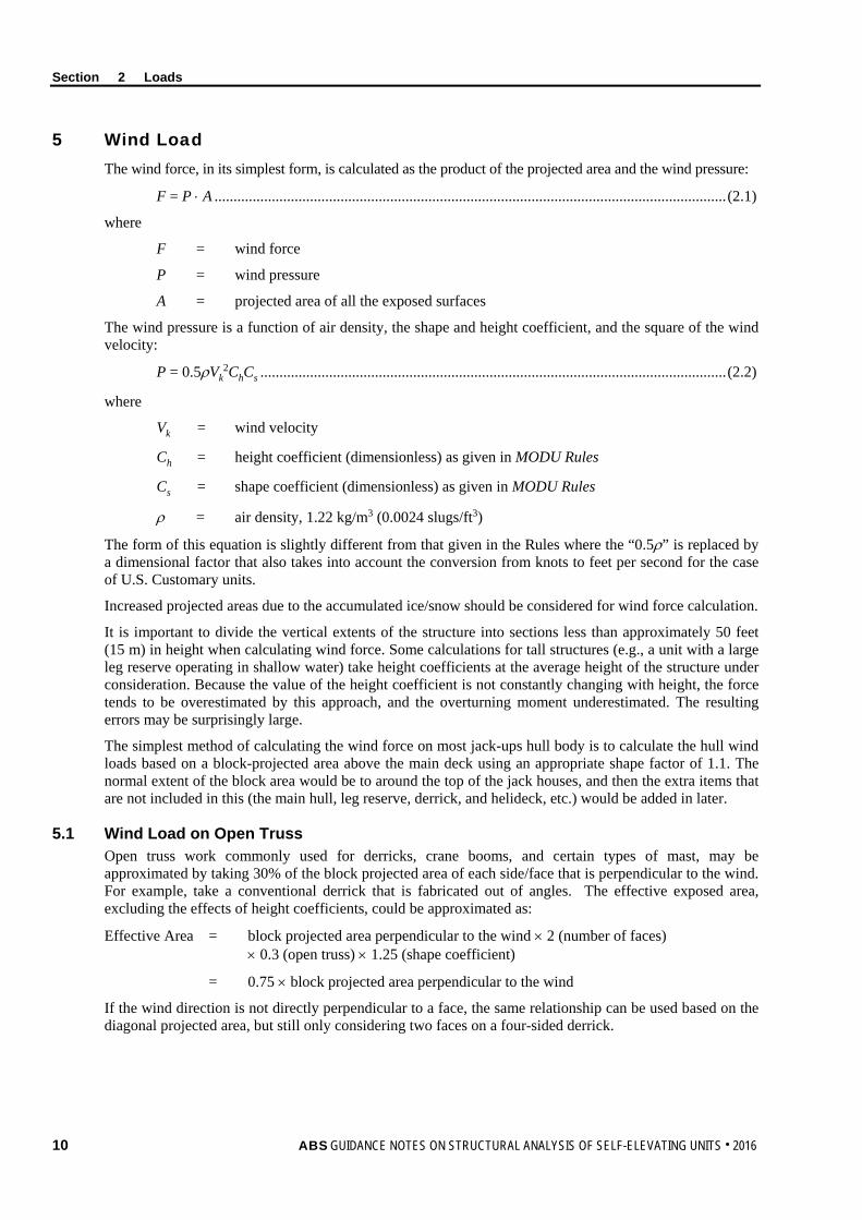
5 Wind Load The wind force, in its simplest form, is calculated as the product of the projected area and the wind pressure:
F = P ⋅ A ...................................................................................................................................... (2.1)
where
F = wind force
P = wind pressure
A = projected area of all the exposed surfaces
The wind pressure is a function of air density, the shape and height coefficient, and the square of the wind velocity:
P = 0.5ρVk2ChCs .......................................................................................................................... (2.2)
where
Vk = wind velocity
Ch = height coefficient (dimensionless) as given in MODU Rules
Cs = shape coefficient (dimensionless) as given in MODU Rules
ρ = air density, 1.22 kg/m3 (0.0024 slugs/ft3)
The form of this equation is slightly different from that given in the Rules where the “0.5ρ” is replaced by a dimensional factor that also takes into account the conversion from knots to feet per second for the case of U.S. Customary units.
Increased projected areas due to the accumulated ice/snow should be considered for wind force calculation.
It is important to divide the vertical extents of the structure into sections less than approximately 50 feet (15 m) in height when calculating wind force. Some calculations for tall structures (e.g., a unit with a large leg reserve operating in shallow water) take height coefficients at the average height of the structure under consideration. Because the value of the height coefficient is not constantly changing with height, the force tends to be overestimated by this approach, and the overturning moment underestimated. The resulting errors may be surprisingly large.
The simplest method of calculating the wind force on most jack-ups hull body is to calculate the hull wind loads based on a block-projected area above the main deck using an appropriate shape factor of 1.1. The normal extent of the block area would be to around the top of the jack houses, and then the extra items that are not included in this (the main hull, leg reserve, derrick, and helideck, etc.) would be added in later.
5.1 Wind Load on Open Truss Open truss work commonly used for derricks, crane booms, and certain types of mast, may be approximated by taking 30% of the block projected area of each side/face that is perpendicular to the wind. For example, take a conventional derrick that is fabricated out of angles. The effective exposed area, excluding the effects of height coefficients, could be approximated as:
Effective Area = block projected area perpendicular to the wind × 2 (number of faces) × 0.3 (open truss) × 1.25 (shape coefficient)
= 0.75 × block projected area perpendicular to the wind
If the wind direction is not directly perpendicular to a face, the same relationship can be used based on the diagonal projected area, but still only considering two faces on a four-sided derrick.
10 ABS GUIDANCE NOTES ON STRUCTURAL ANALYSIS OF SELF-ELEVATING UNITS . 2016
Section 2 Loads
5.3 Wind Load on Leg The lattice legs of an SEU should not be treated as open trusses when calculating the wind loads. In general, the same drag coefficient should be used for the calculation of wind loads as hydrodynamic loads, although it is generally acceptable to assume that any tubular member in the reserve of the leg is smooth, with a drag coefficient of 0.5. Drag coefficients of other members should be based on wind tunnel tests, or recognized sources.
5.5 Dynamic Effects and Vortex Induced Vibration The effects of wind spectra and other short-term variation in wind velocity on the response of SEU need not normally be considered, except in special cases of particularly flexible or sensitive structures.
Most of the members in a lattice leg are sufficiently stiff so that vortex-induced-vibration (VIV) generated by wind will not to be an issue. However, there have been cases in which the internal horizontal diagonals are slender enough to be excited in steady winds. The same phenomenon has been noted on some slender helideck bracing members. There is also a potential for VIV on some braces of the newer designs that feature slender “X” braces. The checks for VIV can be complex, but there are a number of simple checks that will give an indication of the propensity for VIV. If the propensity exists, a more detailed analysis may be warranted.
If VIV is found to be an issue, it is important to use the correct level of damping when undertaking an assessment. Generally, low displacement structural damping is extremely small, but it is possible that joint flexibility may increase damping.
7 Wave and Current Loads This Subsection will address direct calculation of wave loads for a conventional quasi-static analysis. Dynamic effects and their determination are discussed in Section 4 of these Guidance Notes.
7.1 Validity and Application of the Morison’s Equation Most SEUs can be adequately assessed using the Morison equation, which is generally considered viable in the analysis of members/legs in which the member diameter is no greater than 20% of the wave length. For SEUs with lattice legs, in which there is normally relatively little shielding, virtually all waves can be assessed using Morison’s equation, although it may be necessary to use a rather detailed equivalent leg model for very short period waves.
The Morison’s equation models the wave force as two components:
FW = FD + FI ............................................................................................................................... (2.3)
The first component is the drag force FD, which is proportional to the square of the water particle’s velocity:
FD = 0.5ρ ⋅ CD ⋅ D ⋅ un ⋅ |un| ......................................................................................................... (2.4)
where
ρ = density of fluid surrounding the member
un = water particle velocity normal to the structural member
|un| = absolute value for water particle velocity normal to the structural member
CD = drag coefficient
D = projected width (diameter for a tubular member)
ABS GUIDANCE NOTES ON STRUCTURAL ANALYSIS OF SELF-ELEVATING UNITS . 2016 11
Section 2 Loads
The second component is the mass or inertia force, FI, which is proportional to the water particle’s acceleration.
FI = ρ ⋅ CM ⋅ (π ⋅ D2/4)D ⋅ an ........................................................................................................ (2.5)
where
an = water particle acceleration normal to the structural member
CM = mass coefficient
The general form of the drag and inertia forces, including the effects of structural motions, is given below. In the case of a rigid structure, the structural velocity and acceleration are set to zero.
FW = 0.5ρDCD(un – nu′ )|un – nu′ | + ρ(πD2/4)[CMan – (CM – 1) na′ ] ............................................. (2.6)
where
un = component of wave and current induced water particle velocity vector normal to the axis of the member
nu′ = component of the velocity vector of the structural member normal to its axis and in the plane of the water particle velocity of interest
an = component of wave and current induced water particle acceleration vector normal to the axis of the member
na′ = component of the acceleration vector of the structural member normal to its axis and in the plane of the water particle acceleration of interest
Because the drag force is proportional to the square of the water particle velocity, the superposition method is not applicable. Therefore when calculating the hydrodynamic loads it is important to vectorially combine the water particle velocities due to both wave and current.
7.3 Hydrodynamic Coefficients 7.3.1 General
It is evident from Morison’s equation that the values of CD and CM are significant to the determination of wave and current load.
Drag and inertia coefficients vary considerably with cross-section shape, Reynolds number, Keulegan-Carpenter number and surface roughness and should be based on reliable data obtained from literature, model tests or full-scale tests. As such, it should be noted that the drag and inertia coefficients discussed below are appropriate only for the brace (tubular) and chord members used to construct the lattice legs of a jack-up. As stated at the start of Section 2, the parameters given in this section have been chosen as part of a complete system for calculating the deterministic loads on an SEU, and as part of an allowable stress design (ASD) approach. They may not be appropriate for use in other analyses, particularly if undertaking a stochastic dynamic analysis.
7.3.2 Drag Coefficient CD For circular cylindrical members the MODU Rules give specific recommendations for the drag coefficients, CD (i.e., 0.62 if smooth).
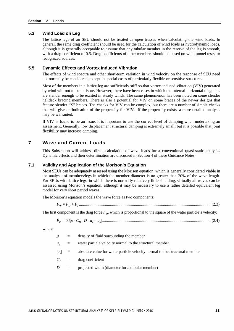
Apart from cylinders, non-tubular members are often used as the chords of an SEU’s legs; some types found in practice are as follows:
• Approximately triangular, with a single rack at the apex of the triangle.
• Double sided rack plate with a half round (or similar) welded on each side of the rack creating a cylindrical chord with a rack through the middle
• Cylindrical with a pair of racks welded to the chord, but offset from the center.
• Cylindrical with non-opposing rack on one side.
12 ABS GUIDANCE NOTES ON STRUCTURAL ANALYSIS OF SELF-ELEVATING UNITS . 2016
Section 2 Loads
FIGURE 1 Non-cylindrical Chords
0θ 0θ0θ 0θ
W W W W
D D DD
Type 1 Type 2 Type 3 Type 4
It needs to be emphasized that there are two kinds of designs for Type 2:
• Double-sided rack plate with a half round welded on each side of the rack creating a cylindrical like chord with a rack through the middle (“split tube” type, D = diameter of tube + Rack Thickness).
• Double-sided rack plate with a less than a half round welded on each side of the rack creating a circular chord with a rack through the middle (“circular” type, D = diameter of tube)
Most of these chords are of the order of 1 meter or less in overall dimension. It is not the intent of this document to give detailed values for each of these leg chord shapes, but to help the analyst decide what an appropriate value to use in the load analysis is.
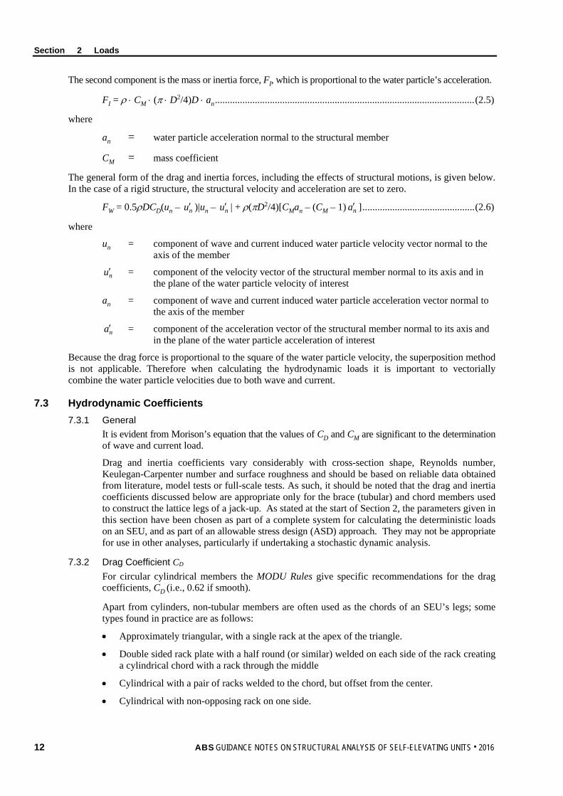
The drag coefficients of most of the irregular shapes are not dependent on the Reynolds number, and are largely unaffected by surface roughness (although increases in diameter due to marine growth should be considered). The drag coefficient depends more on width and depth of the member and changes with the change of flow angle. Section 2, Figure 2 provides the definition of flow angle, θ.
For cylindrical based members (Types 2 to 4), the drag coefficient is similar to that used for a cylinder when flow angle, θ is small. When the flow is perpendicular to the teeth (90° in Section 2, Figure 2) the drag coefficient will be dependent on the size of the rack, but will not be as dependent on whether the tube is smooth or rough. Section 2, Figure 2A shows the shape of curve that could be used to determine the drag coefficient of such a shaped chord. In effect, the drag coefficient is similar to that used for a cylinder for θ is between 0° and 30°, accounting for surface roughness (i.e., 0.62 if smooth, 0.75 if rough). Between 30° and 80° it linearly increases to a plateau level to be used between 80° and 90°. The value at the plateau would vary between 1.5 if the racks do not appreciably increase the overall size of the member, and 2.0 for very large racks. For large diameter tubular legs (as opposed to chords) with attached racks, the upper plateau level could be reduced to 1.2. All the values suggested incorporate a reduction factor to account for the over-prediction of particle kinematics inherent in a deterministic analysis using Stokes fifth order wave theory, or similar. Larger values would need to be used for a stochastic analysis.
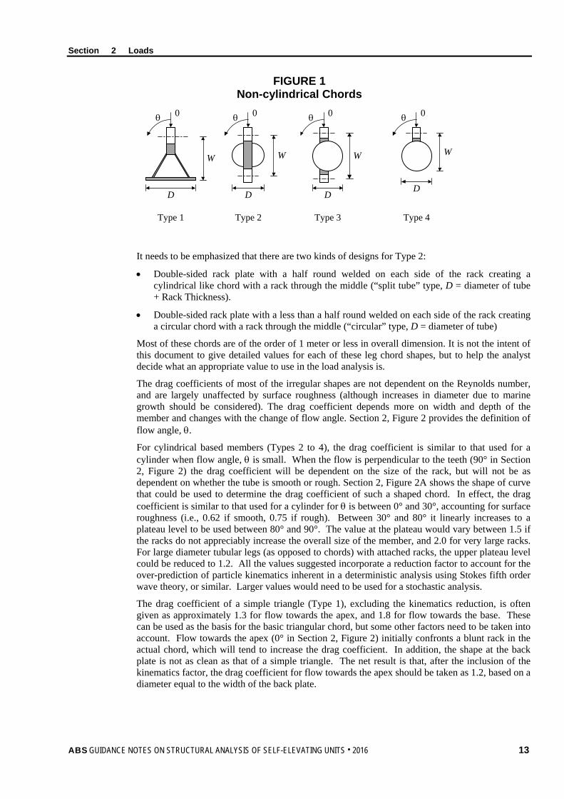
The drag coefficient of a simple triangle (Type 1), excluding the kinematics reduction, is often given as approximately 1.3 for flow towards the apex, and 1.8 for flow towards the base. These can be used as the basis for the basic triangular chord, but some other factors need to be taken into account. Flow towards the apex (0° in Section 2, Figure 2) initially confronts a blunt rack in the actual chord, which will tend to increase the drag coefficient. In addition, the shape at the back plate is not as clean as that of a simple triangle. The net result is that, after the inclusion of the kinematics factor, the drag coefficient for flow towards the apex should be taken as 1.2, based on a diameter equal to the width of the back plate.
ABS GUIDANCE NOTES ON STRUCTURAL ANALYSIS OF SELF-ELEVATING UNITS . 2016 13
Section 2 Loads
As θ increases, initially the coefficient remains flat for approximately 20°, but then it starts to increase. At around 70° (depending on the details of the shape) the maximum projected face is exposed. The shape is also reentrant, so the drag coefficient will increase to a maximum value of approximately 1.75. It will then start to decrease again until the back of the back plate becomes the apex of the triangle. Finally, the coefficient for flow towards the back plate will be 1.5. These values are shown in Section 2, Figure 2B. It must be borne in mind that these are generalized numbers that will not be appropriate for all triangular chord shapes, and the real shape of the graph will be rounded, without abrupt changes of angle at the various change points.
FIGURE 2A Drag Coefficient of Tubular Chord with Rack: Deterministic Analysis
30° 80° 90°
D
W
0°
CD as for Tube
CD
Angle of Flow (away from in line with Rack)
Plateau CD depends on relative size of rack. W/D
FIGURE 2B Drag Coefficient of Triangular Chords: Deterministic Analysis
0 18020 40 60 80 100 120 140 1601
2
1.2
1.4
1.6
1.8
Angle of Flow
Dra
g C
oeff
icie
nt
Typically, the sections of a leg chord are non-tubular, but they are often modeled as a tubular member in analysis having the product of an equivalent diameter and direction dependent hydrodynamic coefficients for various flow directions. Formulas (2.9) thru (2.12) below are for calculating the hydrodynamic coefficients of the equivalent tubular. Several comments about these formulas are as follows.
14 ABS GUIDANCE NOTES ON STRUCTURAL ANALYSIS OF SELF-ELEVATING UNITS . 2016
Section 2 Loads
• The wave/current approach angle plays an important role; angle selection should cover all possibilities.
• There are two kinds of tubular-like chords; one is “split-tube” and the other is “circular” one. This will lead to different CD values.
• The most reliable hydrodynamic coefficients for these non-cylindrical members will be obtained from verified model testing.
7.3.3 Inertia Coefficient CM The Rules specify that the inertia coefficient, Cm, for a tubular should be taken as 1.8. It is of note that, unlike the drag coefficient, the inertia coefficient for tubes decreases as the roughness increases, but similar to drag, both coefficients decrease with increasing Keulegan Carpenter number. This explains the difference between the value given in the Rules, and the theoretical value of 2.
For other shapes, a Cm of 2.0 should be used, based on an effective diameter of tubular that creates the same volume per unit length as the member.
The inertia coefficient does not normally have a significant impact on the loads of a lattice leg SEU, particularly in the severe storm condition. The times that it can be important are in fatigue analyses, on units with large diameter tubular legs, and on units operating in relatively shallow water when the spudcan takes up a significant portion of the water depth.
If it transpires that the inertia coefficient is significant for a specific unit, or area of operations, then consideration will be given to evidence of changed values from those given above.
7.3.4 Appurtenances There are a number of appurtenances that are often attached to the legs of an SEU. The most common are anodes, ladders, jetting lines, gusset plates, and raw water towers. Many of these are small, and can be incorporated through the use of minor conservatism in the calculation, but other items can be of significant size.
Anodes, ladders, and jetting lines, as long as none of them is too large, can normally be incorporated implicitly by using node-to-node length for members, rather than allowing for the reduction in length due to the joint sizes, when creating the hydrodynamic model of the leg.
Gusset plates can have a significant impact on the effective drag coefficient of a leg, and should be considered carefully. Unless they are very small, it is advisable to calculate their effect on the hydrodynamic coefficients of the leg. The drag coefficient recommended for gusset plates is 2.0, but shielding effect can be taken into account. This is particularly significant for legs with high drag chords. These chords severely disrupt fluid flow, so gusset plates often get heavily shielded. Care should be taken when considering the effects of gusset plates on legs with tubular chords as it is possible for a gusset plate to locally increase the effective drag coefficient of the chord by a factor of three. Rarely would there be such an increase on a triangular chord because the initial drag coefficient is already high.
Another item that can significantly affect leg forces is the raw water tower. In the past these were normally independent structures that were cantilevered from the hull down to below the water surface. As such, they attracted some wave load, but in many cases it was not too significant because of the spatial separation from the legs, and because they were relatively small. However many modern units incorporate the tower into the leg. Therefore considerable care should therefore be taken in ensuring that the pipes and guides are properly accounted for when calculating the hydrodynamic loads. Usually it is not the raw water piping itself that attracts the majority of the load, but the guide system, which runs the full extent of the leg.
ABS GUIDANCE NOTES ON STRUCTURAL ANALYSIS OF SELF-ELEVATING UNITS . 2016 15
Section 2 Loads
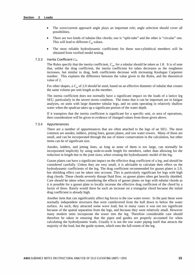
7.3.5 The Hydrodynamic Leg Model – Detailed and Equivalent Leg Total wave loads can be calculated using a detailed or equivalent hydrodynamic leg model. The hydrodynamic coefficients (CD and CM) of individual tubular and non-tubular members that comprise the leg were discussed in 2/7.3.1 and 2/7.3.2. Detailed model is required for the SEU analysis in step 2 of the quasi-static analysis for performing the “unity checks”. Since the member elements used to represent the legs in most software have structural and hydrodynamic properties, thus, the detailed leg model is normally used for hydrodynamic and structural calculations at the same time.
However, it is common practice to use an equivalent leg in analysis to reduce computational effort, especially for the nonlinear time domain dynamic analysis, which can be very time-consuming. It will be necessary to determine the hydrodynamic properties of the equivalent leg. This can be done by using a wave force program to analyze an entire leg bay in a uniform current. Alternatively, manual calculation as described below may be used.
The hydrodynamic properties of a lattice leg in the “equivalent model” can be represented by an equivalent drag coefficient CDe, an equivalent mass coefficient CMe, and an equivalent diameter De. The following items can be used to determine these equivalent hydrodynamic parameters.
7.3.5(a) Equivalent Diameter. The equivalent diameter, De, of a lattice leg shown in Section 2, Figure 3, can be determined as:
De = ( )∑ sD ii /2 ....................................................................................................... (2.7)
where
De = equivalent diameter of the lattice leg
Di = reference diameter of member i
i = reference length of member i (node to node)
s = height of one bay, or part of bay being considered.
7.3.5(b) Equivalent Drag Coefficient. The equivalent drag coefficient, CDe, of the lattice leg can be determined as:
CDe = ∑ DeiC ............................................................................................................... (2.8)
where
CDei = equivalent drag coefficient of each individual member
= [sin2βi + cos2βi sin2αi]3/2 CDi sD
De
ii
CDi = drag coefficient of an individual member i, related to reference dimension Di
αi = angle between flow direction and member axis projected onto a horizontal plane (see Section 2, Figure 3 below)
βi = angle defining the member inclination from the horizontal plane (see Section 2, Figure 3 below)
Note: “Σ” indicates summation over all members in one leg bay.
16 ABS GUIDANCE NOTES ON STRUCTURAL ANALYSIS OF SELF-ELEVATING UNITS . 2016
Section 2 Loads
FIGURE 3 One Bay of Lattice Leg
sα
β
Flow direction
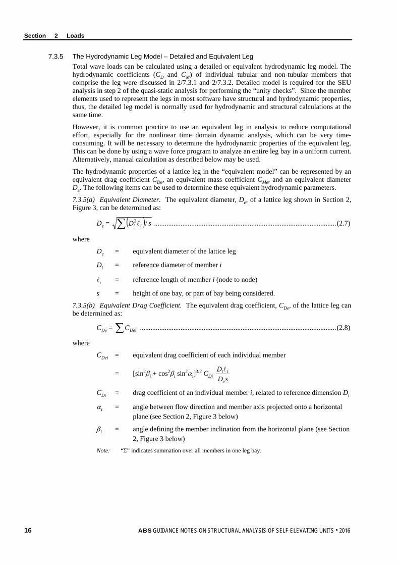
For a split tube chord as shown in Section 2, Figure 4, the drag coefficient CDi, related to the reference dimension Di, may be taken as:
CDi =
°≤θ<°°−θ−+°≤θ<°
9020;]7/9)20[sin)/(200;
2010
0
DiDD
D
CDWCCC
......................... (2.9)
where
θ = angle in degrees, Section 2, Figure 4
CD0 = drag coefficient for a tubular
CD1 = drag coefficient for flow normal to the rack (θ = 90°), related to projected diameter, W
=
<<<+
<
i
ii
i
DWDWDW
DW
/8.1;0.28.1/2.1;)/(3/14.1
2.1/;8.1 .............................................. (2.10)
FIGURE 4 Split-Tube Chord Section
W
D
θ
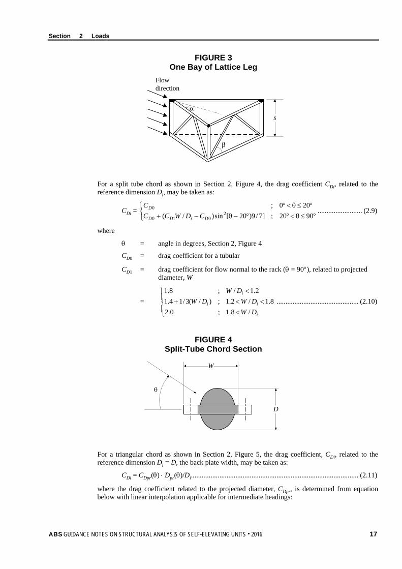
For a triangular chord as shown in Section 2, Figure 5, the drag coefficient, CDi, related to the reference dimension Di = D, the back plate width, may be taken as:
CDi = CDpr(θ) ⋅ Dpr(θ)/Di.............................................................................................. (2.11)
where the drag coefficient related to the projected diameter, CDpr, is determined from equation below with linear interpolation applicable for intermediate headings:
ABS GUIDANCE NOTES ON STRUCTURAL ANALYSIS OF SELF-ELEVATING UNITS . 2016 17
Section 2 Loads
CDpr =
°=θθ−°=θ
°=θ°=θ
°=θ
180;00.2180;65.1105;40.190;95.10;70.1
o
.................................................................................. (2.12)
The projected diameter, Dpr, may be determined from:
Dpr =
<θ<θ−θθ−<θ<θθ+θ
θ<θ<θ
180)180(;|)cos(|)180(;|)cos(|5.0)sin(
0;)cos(
o
oo
o
DDW
D .......................................... (2.13)
The angle θo, where half the rackplate is hidden, θo = tan-1[D/(2W)].
FIGURE 5 Triangular Chord Section
D
W
θ
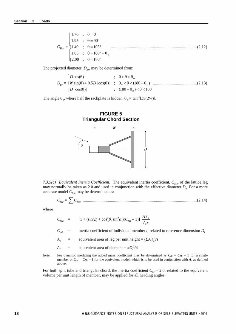
7.3.5(c) Equivalent Inertia Coefficient. The equivalent inertia coefficient, CMe, of the lattice leg may normally be taken as 2.0 and used in conjunction with the effective diameter De. For a more accurate model CMe may be determined as:
CMe = ∑ MeiC ............................................................................................................. (2.14)
where
CMei = [1 + (sin2βi + cos2βi sin2αi)(CMi – 1)] sA
A
e
ii
Cmi = inertia coefficient of individual member i, related to reference dimension Di
Ae = equivalent area of leg per unit height = (ΣAii)/s
Ai = equivalent area of element = πDi2/4
Note: For dynamic modeling the added mass coefficient may be determined as CAi = CMi – 1 for a single member or CAe = CMe – 1 for the equivalent model, which is to be used in conjunction with Ae as defined above.
For both split tube and triangular chord, the inertia coefficient CM = 2.0, related to the equivalent volume per unit length of member, may be applied for all heading angles.
18 ABS GUIDANCE NOTES ON STRUCTURAL ANALYSIS OF SELF-ELEVATING UNITS . 2016
Section 2 Loads
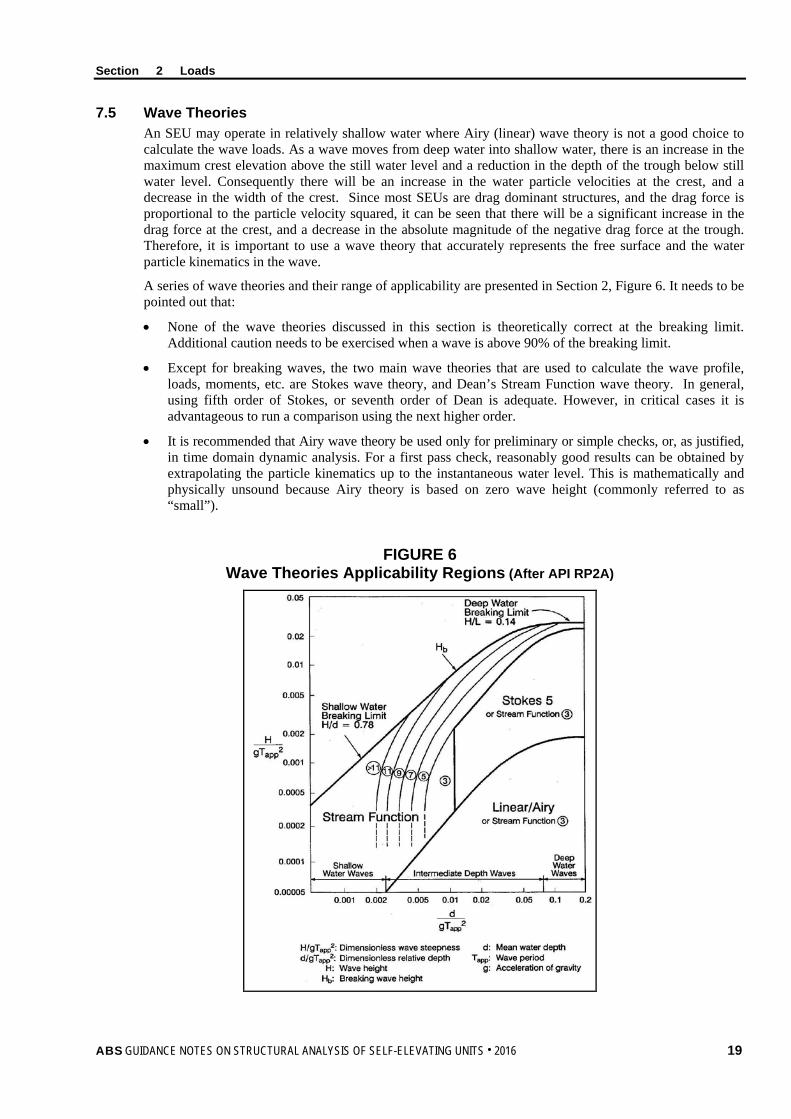
7.5 Wave Theories An SEU may operate in relatively shallow water where Airy (linear) wave theory is not a good choice to calculate the wave loads. As a wave moves from deep water into shallow water, there is an increase in the maximum crest elevation above the still water level and a reduction in the depth of the trough below still water level. Consequently there will be an increase in the water particle velocities at the crest, and a decrease in the width of the crest. Since most SEUs are drag dominant structures, and the drag force is proportional to the particle velocity squared, it can be seen that there will be a significant increase in the drag force at the crest, and a decrease in the absolute magnitude of the negative drag force at the trough. Therefore, it is important to use a wave theory that accurately represents the free surface and the water particle kinematics in the wave.
A series of wave theories and their range of applicability are presented in Section 2, Figure 6. It needs to be pointed out that:
• None of the wave theories discussed in this section is theoretically correct at the breaking limit. Additional caution needs to be exercised when a wave is above 90% of the breaking limit.
• Except for breaking waves, the two main wave theories that are used to calculate the wave profile, loads, moments, etc. are Stokes wave theory, and Dean’s Stream Function wave theory. In general, using fifth order of Stokes, or seventh order of Dean is adequate. However, in critical cases it is advantageous to run a comparison using the next higher order.
• It is recommended that Airy wave theory be used only for preliminary or simple checks, or, as justified, in time domain dynamic analysis. For a first pass check, reasonably good results can be obtained by extrapolating the particle kinematics up to the instantaneous water level. This is mathematically and physically unsound because Airy theory is based on zero wave height (commonly referred to as “small”).
FIGURE 6 Wave Theories Applicability Regions (After API RP2A)
ABS GUIDANCE NOTES ON STRUCTURAL ANALYSIS OF SELF-ELEVATING UNITS . 2016 19
Section 2 Loads
There are two critical phenomena that need to be dealt with cautiously for wave calculation. The first is the nonlinearity of waves. This happens for many reasons, but mainly from the asymmetry of the wave profile. The wave spreading effect also influences the height of a wave in different directions. The second is the irregularity, or random nature of waves.
Airy wave theory is usually used for stochastic analysis requiring linearity. For time domain analysis in a random sea state, the Airy wave is used because the creation of random wave history requires the superposition of wave components. Ignoring nonlinearity should be compensated by some appropriate modifications or adjustments.
Nonlinear wave theories (e.g., Stoke 5th or Dean Stream) usually are used in deterministic analysis. The specific values of wave height and period are specified by the Owner.
7.7 Asymmetry As mentioned above, Airy wave theory is used in some cases. It could underestimate the wave load due to ignoring the asymmetry of the wave profile (crest greater than trough). For the fatigue analysis, such underestimation may be ignored because the highest wave components only produce a small part of total damage. However, for the case of stochastic analysis in the time domain (see also Section 4), the wave height should be adjusted as follows in lieu of using a nonlinear wave theory.
Hs = [1 + 0.5e(–d/25)]Hsrp (d ≥ 25 m) ........................................................................... (2.15)
where
d = water depth, in meters
Hs = stochastic design significant wave height
Hsrp = significant wave height
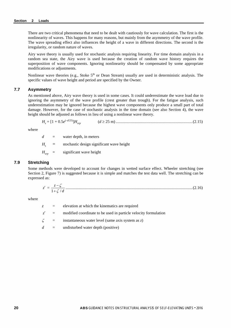
7.9 Stretching Some methods were developed to account for changes in wetted surface effect. Wheeler stretching (see Section 2, Figure 7) is suggested because it is simple and matches the test data well. The stretching can be expressed as:
z′ = d
z/1 ζζ
+− ............................................................................................................................ (2.16)
where
z = elevation at which the kinematics are required
z′ = modified coordinate to be used in particle velocity formulation
ζ = instantaneous water level (same axis system as z)
d = undisturbed water depth (positive)
20 ABS GUIDANCE NOTES ON STRUCTURAL ANALYSIS OF SELF-ELEVATING UNITS . 2016
Section 2 Loads
FIGURE 7 Wheeler Stretching of Wave
Airy theory sinusoidal wave
Velocity/acceleration profile according to Wheeler
Velocity/acceleration profile
This approach is similar to the stretch/compression of current profile in combination with wave; however, they are two totally different phenomena.
7.11 Shielding Depending on the configuration of the leg structures, the forces on leg structural members may be reduced due to hydrodynamic shielding. However, the shielding reduction of wave force acting on an SEU leg is usually insignificant because of the relatively open arrangement of the leg members in space. As a result, it is unusual to include shielding reductions in an SEU analysis.
7.13 Wave Approach Angle Except for fatigue analysis, the wave conditions used for SEU analysis in the elevated mode are usually assumed as omni-direction. Nevertheless, different approach angles have to be selected for determining the wave loads because of the asymmetry of many parameters in the geometry of leg. The following factors should be considered when determining the wave approach angles:
• The arrangement of the legs
• The arrangement of the chords of leg
• The orientation of member in both leg and chord level, especially for 4 chord leg design.
7.15 Breaking Wave and Slamming Based on the design water depth, the breaking wave limit can be calculated according Figure 6. It is important for a designer to check whether the design wave is above a breaking wave limit and to use the appropriate wave theory accordingly.
When assessing an SEU in breaking wave conditions, considerable care should be exercised to ensure that the wave loads are not underestimated. The fluid flow past the member is not continuous: a breaking wave is more akin to slamming on the member in a vertical plane, particularly those parallel to the wave crest. Slamming force can be evaluated by:
FS = 0.5ρ ⋅ CS ⋅ D ⋅ u2 ................................................................................................................ (2.19)
where
ρ = density of fluid surrounding the tubular
u = water particle velocity normal to the structural member
Airy theory sinusoidal wave
ABS GUIDANCE NOTES ON STRUCTURAL ANALYSIS OF SELF-ELEVATING UNITS . 2016 21
Section 2 Loads
CS = slam coefficient
= π with dynamic effect
= 5.5 without dynamic effect
D = projected width (diameter for tubular member)
The total structural loads may not be much higher than those generated using an equivalent leg and normal steady flow because the wave crest is so narrow that it will only affect a small part of the leg at a time as it passes through it. Units with large diameter tubular legs should be carefully considered, as there could be significant transient effects. [Additional guidance on slamming is given in Part 5B, Appendix 1, “Wave Impact Criteria” of the ABS Rules for Building and Classing Floating Production Installations”]
In a fatigue analysis, the breaking wave loads and slamming loads on horizontal members near the water surface are more important. If steady flow is used in the analysis, the fatigue loads could be significantly underestimated.
7.17 Stepping Wave through Structures When analyzing an SEU, it is a normal practice to step the wave through the structure in order to capture the maximum wave force and overturning moment. The length of the phase step will depend on the steepness of the wave, but a five-degree step is normally sufficient for all but the steepest waves. In steep waves it is advantageous to have a final step through with one-degree steps.
The unit is then assessed at the phase angle where base shear is maximized and the phase angle where overturning moment is maximized.
9 Large Displacement Load (P-∆ Effect) SEUs are flexible structures subject to relatively high lateral displacements, especially from environmental loading. These displacements result in a lateral offset of each leg from the base of the leg to the hull level of the legs. This offset leads to an additional moment in the leg, the P-∆ moment, or the so-called P-∆ load (where P is the load in each individual leg, and Δ is the lateral displacement at the hull level). For a unit operating in a deep water field, there can be significant lateral displacement at the hull level. The consequences of the P-∆ effect are as follows.
• Increased overturning moment
• Increased hull side sway, the increased deflection is a function of the ratio of the applied axial load to the Euler load
• Increased axial load in leeward leg while reduced axial load in windward leg
• Redistribution of shear forces in legs.
P-∆ load should therefore be considered in the design of an SEU. There are various ways to account for P-∆ load, as described below.
9.1 Large Displacement Method The first method and the most comprehensive one, is the large displacement method. Sometimes it is also called “geometric nonlinearity” in FEM analysis. In such methods the nonlinearity (large-displacement) is obtained by applying the load in increments and iteratively generating the stiffness matrix for the next load increment from the deflected shape of the previous increment until the response converges (error within certain range). Nevertheless the accuracy is obtained at the cost of computational effort.
9.3 Geometric Stiffness Method Other approaches called “geometric stiffness methods”, address the P-∆ effect by introducing a linear adjustment to the element stiffness matrix based on the axial load present in the element.
22 ABS GUIDANCE NOTES ON STRUCTURAL ANALYSIS OF SELF-ELEVATING UNITS . 2016
Section 2 Loads
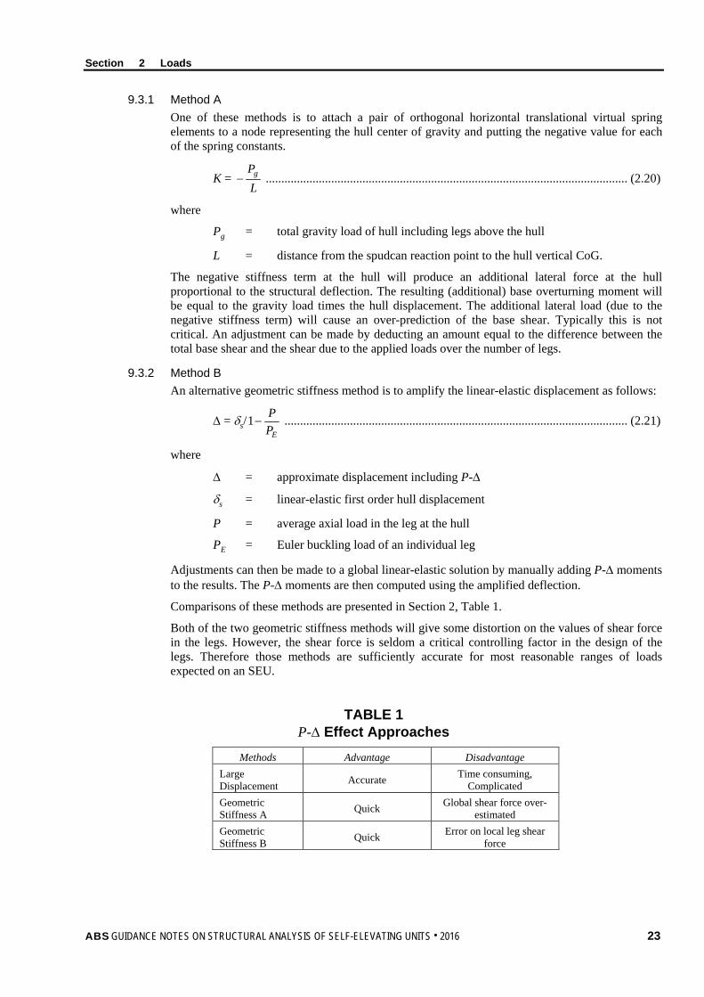
9.3.1 Method A One of these methods is to attach a pair of orthogonal horizontal translational virtual spring elements to a node representing the hull center of gravity and putting the negative value for each of the spring constants.
K = LPg− .................................................................................................................... (2.20)
where
Pg = total gravity load of hull including legs above the hull
L = distance from the spudcan reaction point to the hull vertical CoG.
The negative stiffness term at the hull will produce an additional lateral force at the hull proportional to the structural deflection. The resulting (additional) base overturning moment will be equal to the gravity load times the hull displacement. The additional lateral load (due to the negative stiffness term) will cause an over-prediction of the base shear. Typically this is not critical. An adjustment can be made by deducting an amount equal to the difference between the total base shear and the shear due to the applied loads over the number of legs.
9.3.2 Method B An alternative geometric stiffness method is to amplify the linear-elastic displacement as follows:
∆ = δs/EP
P−1 .............................................................................................................. (2.21)
where
∆ = approximate displacement including P-∆
δs = linear-elastic first order hull displacement
P = average axial load in the leg at the hull
PE = Euler buckling load of an individual leg
Adjustments can then be made to a global linear-elastic solution by manually adding P-∆ moments to the results. The P-∆ moments are then computed using the amplified deflection.
Comparisons of these methods are presented in Section 2, Table 1.
Both of the two geometric stiffness methods will give some distortion on the values of shear force in the legs. However, the shear force is seldom a critical controlling factor in the design of the legs. Therefore those methods are sufficiently accurate for most reasonable ranges of loads expected on an SEU.
TABLE 1 P-∆ Effect Approaches
Methods Advantage Disadvantage Large Displacement Accurate Time consuming,
Complicated Geometric Stiffness A Quick Global shear force over-
estimated Geometric Stiffness B Quick Error on local leg shear
force
ABS GUIDANCE NOTES ON STRUCTURAL ANALYSIS OF SELF-ELEVATING UNITS . 2016 23
Section 2 Loads
11 Dynamic Load (Inertial Effect) When pursuing the two-step dynamic analysis approach that is described in Section 4 of these Guidance Notes, the dynamic response can be modeled as a set of inertial loads applied in the quasi-static analysis.
11.1 Magnitude of Inertial Load The magnitude of inertial load can be obtained from:
Fin = (DAF – 1) ⋅ FSta ................................................................................................................. (2.22)
where
Fin = inertial load
DAF = Dynamic Amplification Factor
FSta = static load
The DAF is defined as the ratio of dynamic response to static response. DAFs can be quantified for various structural responses, such as the global overturning moment (OTM) of the unit, base shear (BS) force or the lateral displacement of the elevated hull (i.e., surge and sway) and leg bending moment at lower guide. The OTM and BS are the two most commonly used responses.
11.3 Distribution of Inertial Load The inertial load can be applied on the structural model either in a simplified manner or in a more detailed method.
For the simplified approach, an inertial point load is applied at the CoG of hull in the down-wind direction using the DAF for base shear.
In the more detailed method, a set of inertial loads is applied to the quasi-static structural analysis model based on the mass distribution and mode shapes of the structures.
A comprehensive discussion of inertial loads is presented in Section 4.
13 Leg Inclination Ordinarily leg inclination is not considered in the Classification of the unit. The major exception would be for a mat supported unit where an Owner-specified out-of-level is provided. Under these circumstances, the inclination resulting from the specified out-of-level condition should be incorporated into the structural analysis.
24 ABS GUIDANCE NOTES ON STRUCTURAL ANALYSIS OF SELF-ELEVATING UNITS . 2016
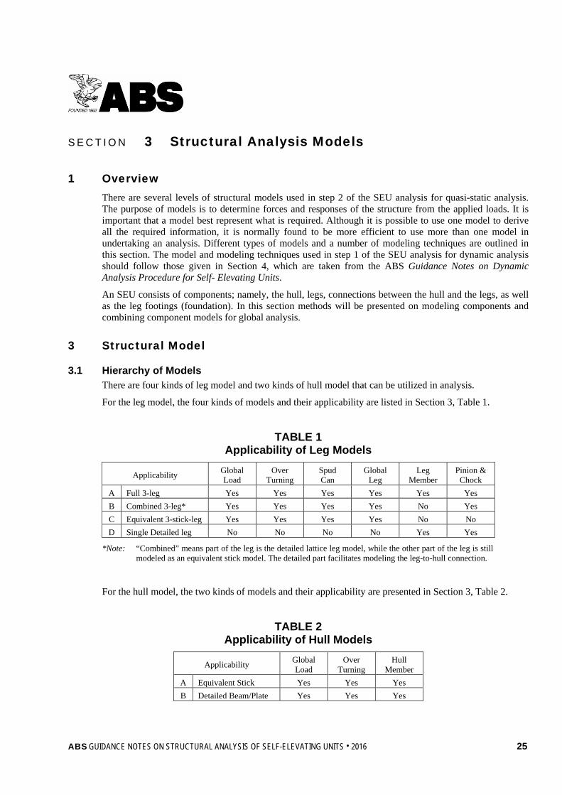
S e c t i o n 3 : S t r u c t u r a l A n a l y s i s M o d e l s
S E C T I O N 3 Structural Analysis Models
1 Overview There are several levels of structural models used in step 2 of the SEU analysis for quasi-static analysis. The purpose of models is to determine forces and responses of the structure from the applied loads. It is important that a model best represent what is required. Although it is possible to use one model to derive all the required information, it is normally found to be more efficient to use more than one model in undertaking an analysis. Different types of models and a number of modeling techniques are outlined in this section. The model and modeling techniques used in step 1 of the SEU analysis for dynamic analysis should follow those given in Section 4, which are taken from the ABS Guidance Notes on Dynamic Analysis Procedure for Self- Elevating Units.
An SEU consists of components; namely, the hull, legs, connections between the hull and the legs, as well as the leg footings (foundation). In this section methods will be presented on modeling components and combining component models for global analysis.
3 Structural Model
3.1 Hierarchy of Models There are four kinds of leg model and two kinds of hull model that can be utilized in analysis.
For the leg model, the four kinds of models and their applicability are listed in Section 3, Table 1.
TABLE 1 Applicability of Leg Models
Applicability Global Load
Over Turning
Spud Can
Global Leg
Leg Member
Pinion & Chock
A Full 3-leg Yes Yes Yes Yes Yes Yes B Combined 3-leg* Yes Yes Yes Yes No Yes C Equivalent 3-stick-leg Yes Yes Yes Yes No No D Single Detailed leg No No No No Yes Yes
*Note: “Combined” means part of the leg is the detailed lattice leg model, while the other part of the leg is still modeled as an equivalent stick model. The detailed part facilitates modeling the leg-to-hull connection.
For the hull model, the two kinds of models and their applicability are presented in Section 3, Table 2.
TABLE 2 Applicability of Hull Models
Applicability Global Load
Over Turning
Hull Member
A Equivalent Stick Yes Yes Yes B Detailed Beam/Plate Yes Yes Yes
ABS GUIDANCE NOTES ON STRUCTURAL ANALYSIS OF SELF-ELEVATING UNITS . 2016 25
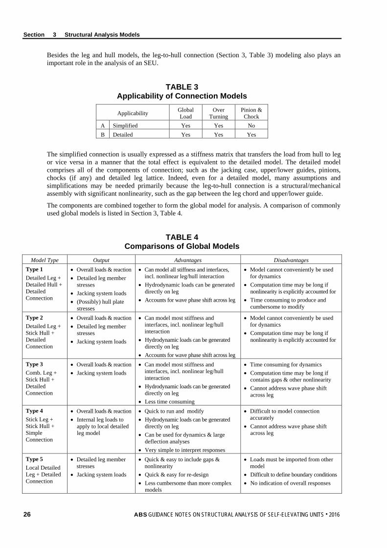
Section 3 Structural Analysis Models
Besides the leg and hull models, the leg-to-hull connection (Section 3, Table 3) modeling also plays an important role in the analysis of an SEU.
TABLE 3 Applicability of Connection Models
Applicability Global Load
Over Turning
Pinion & Chock
A Simplified Yes Yes No B Detailed Yes Yes Yes
The simplified connection is usually expressed as a stiffness matrix that transfers the load from hull to leg or vice versa in a manner that the total effect is equivalent to the detailed model. The detailed model comprises all of the components of connection; such as the jacking case, upper/lower guides, pinions, chocks (if any) and detailed leg lattice. Indeed, even for a detailed model, many assumptions and simplifications may be needed primarily because the leg-to-hull connection is a structural/mechanical assembly with significant nonlinearity, such as the gap between the leg chord and upper/lower guide.
The components are combined together to form the global model for analysis. A comparison of commonly used global models is listed in Section 3, Table 4.
TABLE 4 Comparisons of Global Models
Model Type Output Advantages Disadvantages Type 1 Detailed Leg + Detailed Hull + Detailed Connection
• Overall loads & reaction • Detailed leg member
stresses • Jacking system loads • (Possibly) hull plate
stresses
• Can model all stiffness and interfaces, incl. nonlinear leg/hull interaction
• Hydrodynamic loads can be generated directly on leg
• Accounts for wave phase shift across leg
• Model cannot conveniently be used for dynamics
• Computation time may be long if nonlinearity is explicitly accounted for
• Time consuming to produce and cumbersome to modify
Type 2 Detailed Leg + Stick Hull + Detailed Connection
• Overall loads & reaction • Detailed leg member
stresses • Jacking system loads
• Can model most stiffness and interfaces, incl. nonlinear leg/hull interaction
• Hydrodynamic loads can be generated directly on leg
• Accounts for wave phase shift across leg
• Model cannot conveniently be used for dynamics
• Computation time may be long if nonlinearity is explicitly accounted for
Type 3 Comb. Leg + Stick Hull + Detailed Connection
• Overall loads & reaction • Jacking system loads
• Can model most stiffness and interfaces, incl. nonlinear leg/hull interaction
• Hydrodynamic loads can be generated directly on leg
• Less time consuming
• Time consuming for dynamics • Computation time may be long if
contains gaps & other nonlinearity • Cannot address wave phase shift
across leg
Type 4 Stick Leg + Stick Hull + Simple Connection
• Overall loads & reaction • Internal leg loads to
apply to local detailed leg model
• Quick to run and modify • Hydrodynamic loads can be generated
directly on leg • Can be used for dynamics & large
deflection analyses • Very simple to interpret responses
• Difficult to model connection accurately
• Cannot address wave phase shift across leg
Type 5 Local Detailed Leg + Detailed Connection
• Detailed leg member stresses
• Jacking system loads
• Quick & easy to include gaps & nonlinearity
• Quick & easy for re-design • Less cumbersome than more complex
models
• Loads must be imported from other model
• Difficult to define boundary conditions • No indication of overall responses
26 ABS GUIDANCE NOTES ON STRUCTURAL ANALYSIS OF SELF-ELEVATING UNITS . 2016
Section 3 Structural Analysis Models
Furthermore, it is a common practice to perform global analysis based on a simplified model to obtain the global load, overall reaction force, sectional force, etc., and then use those derived forces as input for more detailed analysis. For example, the reaction force obtained from global analysis can be used as input loading for the analysis of spudcan. This is an effective approach to perform the analysis quickly without overly compromising the quality of the results.
3.3 Hull Model The hull structures can be modeled either as detailed beams plus plates, or a grillage of simplified equivalent beams.
3.3.1 Detailed Hull Model The detailed hull model usually is the combination of plate elements and beam elements. Some points for special attention are listed below:
• Appropriate modeling of beam member to represent the contribution of girder and other bar-like members
• Appropriate modeling of connections between plate/shell elements and beam elements to avoid inappropriate local stress concentrations.
• Clear differentiation between the weight of modeled structural components and separately input weights (loading)
• Clear differentiation between the loads associated mass (weights) and loads not associated with masses (e.g., hook load). This is important for dynamic analysis
• The accurate assignment of masses to both translational and rotational degrees of freedom. (CoG and moment of inertial of mass)
• An appropriate meshing scheme to obtain balance between accuracy and efficiency
3.3.2 Simplified Hull Model A simplified hull model can be used when the focus of the analysis is not on the response of hull members. It can significantly reduce computational effort, especially for the case of nonlinear dynamic analysis in time domain.
When determining the geometric properties (stiffness) of the equivalent beams, the following points should be observed.
• The beams can be located along the main bulkheads and side shell of the hull
• The flange width of the equivalent beam can be set as effective width of plating.
• The assignment of beam properties in gap and overlap areas should be as balanced as practicable
• The in plane bending stiffness (Iy) can be set very high because of the effective constraint against in-plane bending restraint coming from the contribution of the deck and bottom plating.
The torsional stiffness (J) of the equivalent beam can be calculated as:
J = ∑ )/(
4 2
tbA ................................................................................................................ (3.1)
where
A = box enclosed area
b = width of the calculated side
t = thickness of the calculated side
ABS GUIDANCE NOTES ON STRUCTURAL ANALYSIS OF SELF-ELEVATING UNITS . 2016 27
Section 3 Structural Analysis Models
This method is to calculate the J for a box. In the case of a wide flange beam, the calculated J of the box can be distributed to the wide flange beams as per the width of each section.
An existing practice assumes the stiffness of the equivalent beams as rigid or a very high value for simplicity under the case of dynamic analysis. Although the mass of an SEU is concentrated near the hull body and the stiffness of the hull is much higher than those of legs, this assumption will still somewhat alter the natural periods of the SEU. Consequently the overall dynamic response will be affected as well.
Similarly, when using a simplified hull model, the sum of mass is placed at the CoG of the hull. This approach is adequate in simulating the translational movement of hull. But it may not be adequate to capture the rotational response of hull because it cannot reflect the distribution of mass about the rotational axis. As a result, the impact on the first or second mode may not be significant, but the higher modes will be affected by this simplification.
3.5 Leg Model Three kinds of leg models; namely, detailed model, simplified model and combined model, are used in SEU analysis.
In selecting a type of model appropriate for a specific analysis, special care should be taken when calculating wave loads of very steep waves in shallow water.
An equivalent leg model can produce incorrect loads from steep waves in shallow water, because the crest may be so steep that the wave particle kinematics significantly changes within a very small distance from the wave crest. Such differences cannot be represented by the equivalent leg model, which merely assumes that all members take wave load at the same phase angle.
The maximum wave force determined using an equivalent leg model will be greater than those from a detailed leg model due to these differences.
For fatigue analysis, worst stresses may not be associated with the maximum and minimum wave forces on the unit, which normally occur in the sections around the guides.
3.5.1 Detailed Leg Model A “detailed leg” model consists of all structural members such as chords, horizontal, diagonal and internal braces of the leg structure and the spudcan (if required). Each structural component of the leg is represented by one or more beam elements.
Some special issues for the modeling of detailed legs are listed below:
• The orientation of the chords member should be treated carefully with reference to the hydrodynamic coefficients.
• The secondary components; such as gusset plates, anodes, ladders, should be addressed appropriately since they will also attract hydrodynamic force.
• Overlapped joints (very common in SEU leg design; such as a joint with two diagonal and one horizontal braces) can be modeled as one common joint. This is sufficient for global analysis. However, for the case of a specific joint evaluation, a more detailed model should be used.
• For a joint where there is more than one brace, it is unlikely that there will be one common point of intersection between the braces and chord. An intermediate point between the two intersections with proper member offset setting should be sufficient if the distance of the bracing members is less than one quarter of the diameter of main member. Otherwise two separate joints with one connecting member should be modeled.
• Gusset plates normally need not be included in the structural leg model, but their effects may be taken into account in the strength check of members and joints.
28 ABS GUIDANCE NOTES ON STRUCTURAL ANALYSIS OF SELF-ELEVATING UNITS . 2016
Section 3 Structural Analysis Models
3.5.2 Simplified Leg Model The simplified leg model is a compromise of precision and efficiency. In this model, the leg structure is simulated by a series of collinear beams representing the equivalent overall stiffness characteristics of the detailed leg. The stiffness properties of the leg can be obtained by empirical formulas considering the configuration of the leg. But using computer modeling, the stiffness properties can be obtained in a more straightforward and precise way as described below.
i) Create the detailed leg model.
ii) Fix the model at one end and apply unit loads (in 6 degrees of freedom) at the other end.
iii) Run static analysis to obtain the displacement caused by the unit load.
iv) Compute the stiffness properties of the detailed leg using the unit loads and the corresponding displacements.
3.5.2(a) Unit Axial Load Applied at the End of the Leg. The axial area of the equivalent leg beam may be calculated as:
A = ∆E
FL ........................................................................................................................ (3.2)
where
A = effective axial area of the leg
∆ = axial deflection of cantilever at point of load application
F = applied axial end load
L = length of cantilever (from rigid support to point of load application)
E = Young's modulus
3.5.2(b) Unit Horizontal Load Applied at the End of the Leg. The effective moment of inertia of the leg may be calculated as:
I = θE
PL2
2 ........................................................................................................................ (3.3)
where
I = effective moment of inertia of the leg
P = horizontal load applied at the end of the leg
L = length of leg between point of fixity and the free rotation end
E = young’s modulus
θ = average joint rotation of nodes at the end of the leg
3.5.2(c) Effective Shear Area. The effective shear area can be calculated as:
As = G
PLs∆
...................................................................................................................... (3.4)
where
As = effective leg shear area
G = shearing modulus of elasticity
P = horizontal load applied at the end of the leg
∆s = end deflection due to shear only = ∆T – ∆b
∆T = total deflection of the end nodes
ABS GUIDANCE NOTES ON STRUCTURAL ANALYSIS OF SELF-ELEVATING UNITS . 2016 29
Section 3 Structural Analysis Models
∆b = end deflection due to bending only
= EI
PL3
3
3.5.2(d) Effective Torsional Moment of Inertia. The effective torsional moment of inertia can be calculated as:
J = θ⋅GLMT ....................................................................................................................... (3.5)
where
J = effective torsional moment of inertia of the leg
MT = applied torsional moment
θ = resulting rotational angle about the axis of leg
G = shear modulus
L = length of leg between points of fixity and the free rotation end
The equivalent leg can be modeled using the obtained stiffness properties.
Appendix 1 of these Guidance Notes gives the empirical formula approach which can be used to establish the equivalent leg stiffness properties.
3.5.3 Combined Leg Model As indicated by its name, the combined leg model is a combination of the detailed and simplified leg models. The segment of leg that is near the hull will be modeled in detail while the other parts of the leg are still kept simplified. Adoption of the combined model will facilitate the application of the detailed connection model.
Care is required to ensure an appropriate interface and consistency of boundary conditions at the connections. The “detailed leg”/“equivalent leg” connection should be modeled so that the plane of connection remains a plane after the leg is bent. Rigid connecting members are the way to achieve the “rigid plane”. Nevertheless, connecting members that are too stiff will cause errors due to the abrupt change of stiffness. On the other hand, too soft connecting members will lead to the softening of the whole leg and are therefore inaccurate. A trial and error procedure should be used to determine appropriate stiffness values for connecting members.
3.7 Leg-to-Hull Connection Model The modeling of the leg-to-hull connection is perhaps the most critical and difficult step of structural modeling for SEU analysis. It greatly affects the global stiffness of the unit, and consequently affects the unit’s global response for both static and dynamic conditions.
3.7.1 Overview The connection between leg and hull comprise many components that work together to transfer load from leg to hull or vice versa. These components include:
• The upper and lower guides.
• Pinions
• Fixation (chock, if any)
• Jackcase and its bracings
• Shock pad (if any)
• Segment of leg within the range between upper and lower guides
30 ABS GUIDANCE NOTES ON STRUCTURAL ANALYSIS OF SELF-ELEVATING UNITS . 2016
Section 3 Structural Analysis Models
The complexity of the leg-to-hull connection comes from two main sources. The first is the complexity of the structural configuration; the second is the pronounced nonlinearity existing among the structural components. For the first issue, some empirical formula or the results from a detailed structural model can produce satisfactory results. However, the complexities arising from nonlinearity are much more difficult to deal with; they have to be addressed in an approximate manner with some uncertainties attached.
Some general issues related with the modeling of leg-to-hull connection are discussed below.
3.7.1(a) Load Transfer Path. The axial force in the leg is transferred to the leg by the pinions of the jacking units or fixation system (if any). In the legs, it is mainly taken by the leg chords.
The shear force is mainly transferred to the leg through the upper/lower guides. In the legs, it primarily acts on the bracings members.
The bending moment could be transferred to a leg by both the pinions/fixation system and upper/lower guides. For those moments transferred by pinion and fixation system, they mainly come to the chords of leg in form of coupled vertical forces. For those transferred by upper/lower guide, the leg bracings will take most of the loads in the form of coupled horizontal shear forces. The ratio of these moments transferred via pinions/fixation system to total moments is an important technical indicator of the properties of the leg-to-hull connection, which is sometimes referred to by the symbol, “β”.
3.7.1(b) Pinions & Fixation. Pinions and the fixation system are two ways to transfer moments via vertical chord forces.
For a unit equipped with a fixation system, the chock will be engaged in the unit’s elevated mode to provide the main leg-to-hull load transfer path. For a unit without a fixation system, the pinions still work in the elevated mode. Generally, a fixation system will provide a more rigid connection. The value of “β” for a fixation system is higher than that of a pinion system.
For connections without a fixation system, there are also two kinds of jacking systems. One is the floating jacking system, and the other is the fixed jacking system. The latter provides higher bending moment restraint due to its higher stiffness, and therefore has a greater value of “β”.
When vertical force is transferred from chord rack to pinions, the inclined surface of a rack tooth will create a force component in the horizontal direction. Generally, when the chord is a tubular, the pinions will usually be located on the opposite sides of the chord (“opposed rack” chord) and horizontal force from both sides can balance each other. This is not true for ‘single rack’ chord. With only one rack per chord, the horizontal components will create a local bending moment of chord and compression in the horizontal bracing member. This issue should be accounted for in the analysis (the additional compression force should be modeled).
3.7.1(c) Upper/Lower Guide. In an ideal condition, with no horizontal load, there should be no contact between the upper/lower guide and the leg chords. With the existence of bending member and shearing force in the legs, upper/lower guides could make contact with the chords and consequently change the total pattern of load paths in the leg-to-hull connections.
The factors that have influence on the role played by upper/lower guide are listed as follows:
• The clearance between the guides and chords
• The stiffness of the pinions/chock
• The stiffness of the upper/lower guide
• The distance between upper and lower guides
• Dimensions of leg (chord distance)
The modeling of this kind of nonlinear behavior is discussed below.
ABS GUIDANCE NOTES ON STRUCTURAL ANALYSIS OF SELF-ELEVATING UNITS . 2016 31
Section 3 Structural Analysis Models
3.7.2 Detailed Connections The detailed model of a leg-to-hull connection is created by including each individual structural component exactly in the model. The main difficulty is how to treat the nonlinearity coming from:
• The contact of chord and upper/lower guides
• The backlash of jacking system
• The force distribution/redistribution among pinions (if no fixation system or when it is not engaged)
The detailed modeling considerations are described below:
3.7.2(a) Leg Guides. The three main types of guides:
• Butt up against the leg and act only in one direction (although with an opposing pair, may effectively act in either direction) as commonly used on legs with tubular chords (opposed guide)
• Clamp around a component of the chord; albeit with some effective gap (non-opposed guide)
• Ring type guide, which totally surrounds a tubular or square leg
Important factors to be considered in modeling the guides are as follows.
3.7.2(b) Guide Direction. The first, and fundamental, necessity of modeling is to ensure that the guides act in the correct directions, and ONLY in the correct directions. In many cases this will either entail using guide gaps, or manually checking to ensure there are no unwarranted reactions by releasing the constraints of member at certain directions.
3.7.2(c) Guide Gaps. Another factor that can affect the load sharing between the different guides at a particular level is the differential gap. An absolute guide gap will allow the leg to rotate slightly about a horizontal axis before any guide load comes into effect. This can affect the effective stiffness of the leg to hull interface, but the impact on leg stresses or hull support system loads is more pronounced.
A usual situation with a lattice leg unit is when the guide gaps are large, and the jacking system stiffness is also very large. However, this situation is still not normally amenable to ready solution since the results will be affected by how the legs were lying in the guides prior to passage of the “storm”. A differential guide gap can cause a significant redistribution in the load sharing between the chords.
It is not necessarily vital that gaps, or differential gaps, are modeled (unless they are integral to the working of the design, or are particularly large) but it is important to ensure that the unit is designed in such a way that minor changes in the support regime, or in service changes in guide tolerances, do not result in such a drastic change in load sharing that the unit’s legs would be overloaded. If it is found that a design is particularly sensitive, considerable care needs to be exercised in choosing the various parameters used in the analysis. It should also be borne in mind that gaps are frequently the easiest method of ensuring the guide load paths are modeled appropriately.
3.7.2(d) Guide Stiffness. The stiffness of the guides will affect the load sharing between the vertical and horizontal support systems. When modeling the entire hull as a plated structure, most of the stiffness will be inherently incorporated. If a simplified hull model (grillage deck) is used in analysis, some engineering judgment will be needed. On most units, it is possible to model the upper guide, and its support system (i.e., jackcase and supporting structure, or equivalent) as a simple plated or framed structure, tied into the grillage deck. The lower guide, because of its generally higher stiffness, can be taken directly connected to the grillage deck via a spring. The stiffness of the lower guide spring can be estimated from a brief assessment of the support structure. While errors in lower guide stiffness will affect the results of an analysis, experience has shown that the results are not too sensitive to less than “gross” errors. Since the upper guide is generally tied into the jackcase and supporting structure and tends to be less stiff than the lower guide, it can be responsible for a greater gross rotation of the leg in the guides, and a consequent increase in the load shed to the vertical support mechanism.
32 ABS GUIDANCE NOTES ON STRUCTURAL ANALYSIS OF SELF-ELEVATING UNITS . 2016
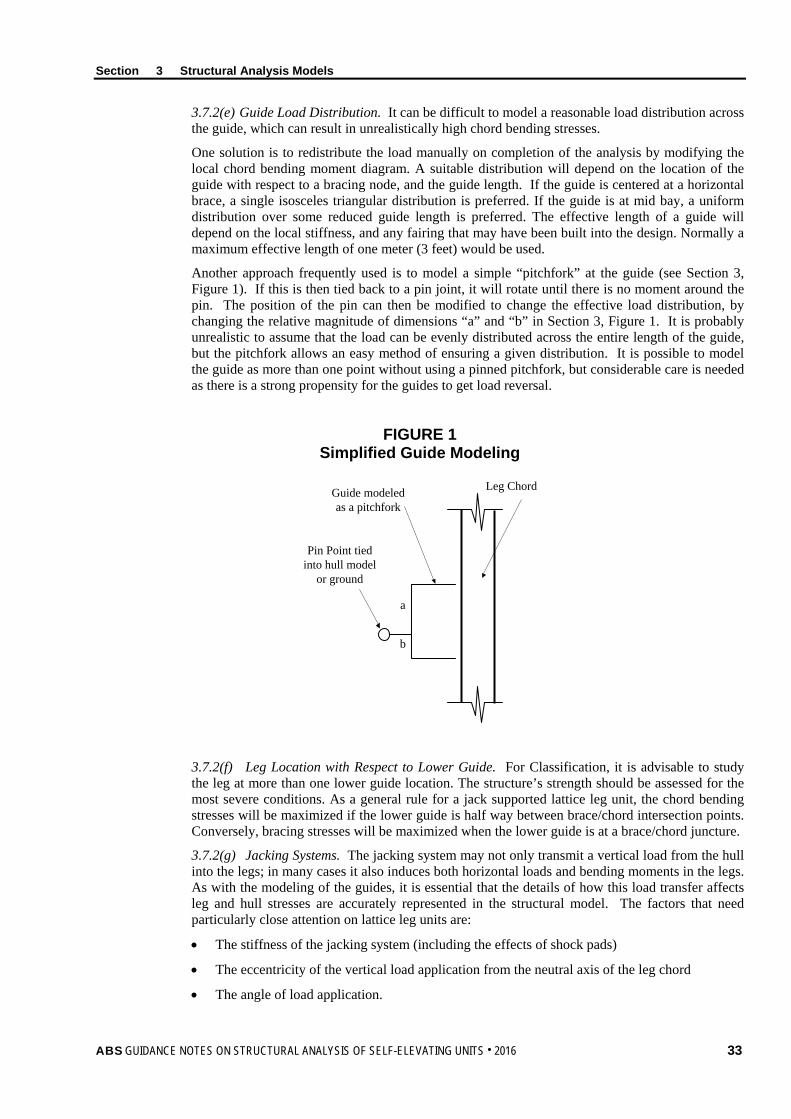
Section 3 Structural Analysis Models
3.7.2(e) Guide Load Distribution. It can be difficult to model a reasonable load distribution across the guide, which can result in unrealistically high chord bending stresses.
One solution is to redistribute the load manually on completion of the analysis by modifying the local chord bending moment diagram. A suitable distribution will depend on the location of the guide with respect to a bracing node, and the guide length. If the guide is centered at a horizontal brace, a single isosceles triangular distribution is preferred. If the guide is at mid bay, a uniform distribution over some reduced guide length is preferred. The effective length of a guide will depend on the local stiffness, and any fairing that may have been built into the design. Normally a maximum effective length of one meter (3 feet) would be used.
Another approach frequently used is to model a simple “pitchfork” at the guide (see Section 3, Figure 1). If this is then tied back to a pin joint, it will rotate until there is no moment around the pin. The position of the pin can then be modified to change the effective load distribution, by changing the relative magnitude of dimensions “a” and “b” in Section 3, Figure 1. It is probably unrealistic to assume that the load can be evenly distributed across the entire length of the guide, but the pitchfork allows an easy method of ensuring a given distribution. It is possible to model the guide as more than one point without using a pinned pitchfork, but considerable care is needed as there is a strong propensity for the guides to get load reversal.
FIGURE 1 Simplified Guide Modeling
a
b
Guide modeled as a pitchfork
Leg Chord
Pin Point tied into hull model
or ground
3.7.2(f) Leg Location with Respect to Lower Guide. For Classification, it is advisable to study the leg at more than one lower guide location. The structure’s strength should be assessed for the most severe conditions. As a general rule for a jack supported lattice leg unit, the chord bending stresses will be maximized if the lower guide is half way between brace/chord intersection points. Conversely, bracing stresses will be maximized when the lower guide is at a brace/chord juncture.
3.7.2(g) Jacking Systems. The jacking system may not only transmit a vertical load from the hull into the legs; in many cases it also induces both horizontal loads and bending moments in the legs. As with the modeling of the guides, it is essential that the details of how this load transfer affects leg and hull stresses are accurately represented in the structural model. The factors that need particularly close attention on lattice leg units are:
• The stiffness of the jacking system (including the effects of shock pads)
• The eccentricity of the vertical load application from the neutral axis of the leg chord
• The angle of load application.
ABS GUIDANCE NOTES ON STRUCTURAL ANALYSIS OF SELF-ELEVATING UNITS . 2016 33
Section 3 Structural Analysis Models
3.7.2(h) Jacking System Stiffness. The stiffness of the jacking system influences the distribution of loads between the guides and the jacking systems. The bending moment in the leg below the hull is reacted in the hull by the combined effects of guides and jacks. The stiffness of a jacking system can be calculated based on the stiffness of the various components (torsion and bending of pinions and shafts, deformation of jack support structure, bending in rack and pinion teeth, etc.).
If information about jacking system stiffness is supplied by a manufacturer, it is important to ascertain not only how values were chosen, but also what has been included in them. It is possible that the manufacturer supplied stiffness may be too high because it has been based on the deflections of the final output pinion, and not the complete system. Conversely, it may be too low because it includes all the flexibility of the jack case structure.
Some units have shock pads above and below the jack case. These pads are generally soft compared to the jacking system, and should be modeled accordingly. It is important to model the stiffness of the pads at the expected level of load that they will experience, if non-linear springs are unavailable. At high loads the stiffness may be relatively close to that of a jacking pinion. In some cases, the elasticity of the pad may deteriorate over time, which should be considered in analysis.
3.7.2(i) Eccentricity of Jacking Load from Chord Center. If jacking loads are not at the centroid of the chord, or symmetrically arranged about it, they will induce a local bending moment in the chord, which should be modeled. The most obvious cases in which a moment is induced are those chords with jacks on one side only (as in the Type 1 chord in in Section 2, Figure 2).
The simplest method of modeling the eccentricity is to use a short ‘dummy’ stub member that runs from the centroid of the chord to the effective point of action of the jacks/pins. The member should be stiff, and the load transfer at the pin/pinion end should be modeled to reflect the load application angle. The model of the pin/pinion system depends on the details for the rest of the support and hull model.
3.7.2(j) Angle of Jacking Reaction. For a rack and pinion jacking system, the line of action force will be at an angle perpendicular to the face of the rack (assuming no friction). The angle is normally between 20 and 30 degrees off vertical. The horizontal load component has little effect in a horizontally opposed jacking system with a solid rack between the jacks. On a horizontally opposed jacking system based on tubular chords/legs, where the rack is not solid, it may be necessary to either reinforce the chord/leg wall, or to install a vertical plate between the racks to resist the crushing load. Without this plate, the chord/leg wall may be over stressed, and it is possible for the tube wall to deform sufficiently to allow the jacks to rotate one or more teeth.
Single sided jacks induce a horizontal load towards the center of the leg. These reactions act like the guide reactions, and induce local chord bending. They can also be responsible for some high bracing stresses adjacent to the pinions. It is one of the main purposes of the internal horizontal bracing to resist these leg-crushing loads, and to help the leg maintain its shape.
3.7.2(k) Fixation Systems. Fixation systems are normally designed to be much stiffer than jacking systems. Modeling of the fixation systems should reflect the stiffness, size, location, and load carrying directions. The fixation systems should be modeled to resist both vertical and horizontal forces based on the stiffness of the vertical and horizontal supports and on the relative location of their associated foundations.
3.7.2(l) Linearization. The leg-to-hull connection model may need to be simplified because of computational limitations. The principle of simplification is to linearize the above-mentioned items. A typical value of stiffness that represents the component mostly at the design load level should be adopted for such simplification.
Elastic springs can be used to simulate the role played by the leg guides. The nonlinearity of the guide can be linearized via two methods:
• One is to adjust the stiffness of spring to such a value that the total resulting displacement will equal the actual one plus the gap under an assumed typical load. Obviously, this is only theoretically correct in a situation where the actual load matches that arising from the assumed conditions.
34 ABS GUIDANCE NOTES ON STRUCTURAL ANALYSIS OF SELF-ELEVATING UNITS . 2016
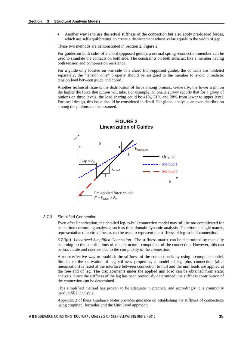
Section 3 Structural Analysis Models
• Another way is to use the actual stiffness of the connection but also apply pre-loaded forces, which are self-equilibrating, to create a displacement whose value equals to the width of gap
These two methods are demonstrated in Section 2, Figure 2.
For guides on both sides of a chord (opposed guide), a normal spring /connection member can be used to simulate the contacts on both side. The constraints on both sides act like a member having both tension and compression resistance.
For a guide only located on one side of a chord (non-opposed guide), the contacts are modeled separately; the “tension only” property should be assigned to the member to avoid unrealistic tension load between guide and chord.
Another technical issue is the distribution of force among pinions. Generally, the lower a pinion the higher the force that pinion will take. For example, an onsite survey reports that for a group of pinions on three levels, the load sharing could be 41%, 31% and 28% from lower to upper level. For local design, this issue should be considered in detail. For global analysis, an even distribution among the pinions can be assumed.
FIGURE 2 Linearization of Guides
Pδ
δ
1
1kactual
kequivalent
Gap = δ0
Pre-applied force coupleF = kactual × δ0
Method 2
Method 1
Original
3.7.3 Simplified Connection Even after linearization, the detailed leg-to-hull connection model may still be too complicated for some time consuming analyses; such as time domain dynamic analysis. Therefore a single matrix, representative of a virtual beam, can be used to represent the stiffness of leg-to-hull connection.
3.7.3(a) Linearized Simplified Connection. The stiffness matrix can be determined by manually summing up the contributions of each structural component of the connection. However, this can be inaccurate and onerous due to the complexity of the connection.
A more effective way to establish the stiffness of the connection is by using a computer model. Similar to the derivation of leg stiffness properties, a model of leg plus connection (after linearization) is fixed at the interface between connection to hull and the unit loads are applied at the free end of leg. The displacements under the applied unit load can be obtained from static analysis. Since the stiffness of the leg has been previously determined, the stiffness contribution of the connection can be determined.
This simplified method has proven to be adequate in practice, and accordingly it is commonly used in SEU analysis.
Appendix 2 of these Guidance Notes provides guidance on establishing the stiffness of connections using empirical formulas and the Unit Load approach.
ABS GUIDANCE NOTES ON STRUCTURAL ANALYSIS OF SELF-ELEVATING UNITS . 2016 35
Section 3 Structural Analysis Models
3.7.3(b) Nonlinear Simplified Connection. A more accurate approach is to include the nonlinearities of the connection.
In this approach, a detailed connection model is created with the nonlinear properties related to stiffness, orientations and clearances. Then, various values of design loads such as axial force, bending moments, etc. are applied in nonlinear analyses, and sets of displacements are obtained. Based on the computed displacements, unique relationships between the connection stiffness and the load levels are obtained.
For global analysis, a simple connection (matrix) model is implemented, but now the matrix is load level dependent. Thus the complicated nonlinear leg-to-hull connection in many degrees of freedom is simplified as a single matrix reflecting nonlinearity.
3.9 Foundation Modeling Typically the foundations of an independent leg SEU are spudcans. Appropriate modeling of the foundation including the boundary conditions simulating the interactions with the seabed soils is important to SEU analysis.
3.9.1 Main Issues For an SEU with spudcans, there are three main issues:
• Penetration evaluation
• Capacity calculation
• Fixity estimation
Foundation issues are primarily thought of as only relating to a site-specific assessment of the unit. For Classification, aspects of the foundation’s behavior such as seabed penetration and soil strength are excluded from the scope of review. The remaining, main foundation issue is related to modeling the restraint or fixity provided by the spudcan/ soil interaction to the structure. Considering this fact, these Guidance Notes will not address geotechnical analysis. Only the penetration and fixity will be addressed below.
3.9.2 Penetration The MODU Rules specify for an independent leg SEU, the lower end of each leg is considered to be at least 3m below the seabed, regardless the site-specific information.
3.9.3 Spudcan Rotational Restraint The boundary conditions of the legs for an independent SEU can be either modeled to be pinned or supported with translational and rotational foundation springs at the reaction points of the spudcans.
Since 2003, the MODU Rules permit consideration of “spudcan-soil rotational stiffness” for cases involving dynamic response. Refer to 4/3.5 and 4/5.3.5 on this topic.
3.9.4 Structural Model For global analysis, the spudcan can be modeled as either a node (corresponding to the simplified leg model) at the reaction point with proper boundary conditions as discussed above, or a beam or plate model corresponding to detailed legs. For the latter case, common practice is still to apply the boundary condition to a single node while connecting this node to the detailed leg by some dummy members (beams or plates). The stiffness of a dummy member should be set appropriately to ensure the proper representation of spudcan stiffness. The spudcan structure should be sufficiently modeled to achieve an accurate load transfer of the seabed reaction to the leg structure. In shallow water depth, a more detailed model may be required.
Care should be taken in interpreting the results of any analyses incorporating highly simplified spudcan models: the member stresses in the vicinity of the spudcan will be greatly influenced because of the rapid change in stiffness.
36 ABS GUIDANCE NOTES ON STRUCTURAL ANALYSIS OF SELF-ELEVATING UNITS . 2016
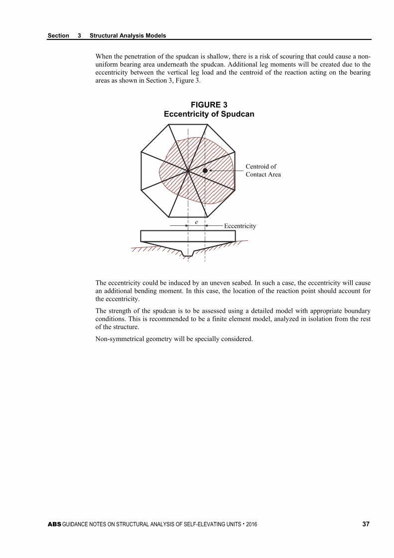
Section 3 Structural Analysis Models
ABS GUIDANCE NOTES ON STRUCTURAL ANALYSIS OF SELF-ELEVATING UNITS . 2016 37
When the penetration of the spudcan is shallow, there is a risk of scouring that could cause a non-uniform bearing area underneath the spudcan. Additional leg moments will be created due to the eccentricity between the vertical leg load and the centroid of the reaction acting on the bearing areas as shown in Section 3, Figure 3.
FIGURE 3 Eccentricity of Spudcan
Eccentricity
Centroid of Contact Area
e
The eccentricity could be induced by an uneven seabed. In such a case, the eccentricity will cause an additional bending moment. In this case, the location of the reaction point should account for the eccentricity.
The strength of the spudcan is to be assessed using a detailed model with appropriate boundary conditions. This is recommended to be a finite element model, analyzed in isolation from the rest of the structure.
Non-symmetrical geometry will be specially considered.
S e c t i o n 4 : S t r u c t u r a l A n a l y s e s
S E C T I O N 4 Structural Analyses
1 Overview The text of the dynamic analysis procedure in this section closely follows that of the ABS Guidance Notes on Dynamic Analysis Procedure for Self-Elevating Units. In those Guidance Notes, the modifications of the site-specific evaluation techniques are described. In the present Guidance Notes, portions of these procedures are repeated below.
1.1 Two-Step Procedure Analysis Because the dynamic response needs to be combined with the static response for assessing the SEU’s strength, the analysis procedure needs first to calculate the dynamic response using dynamic analysis and then to combine the dynamic response with the static response for final assessment of the SEU’s strength. This analysis procedure is referred to as “Two-Step Procedure” and Section 4, Figure 1 shows a flowchart of this procedure. The two-step procedure is summarized as:
i) Use an “equivalent” model to perform a random wave dynamic analysis obtaining the DAFs, and subsequently the inertial load set caused by wave-induced structural dynamics.
Alternatively, the DAFs may also be estimated using the single degree-of-freedom (SDOF) approach given in 4/7.5.1(b) as an alternative to the random wave dynamic analysis, above. However, care should be exercised since the SDOF approach may significantly over or underestimate the DAF. See the limitations of the SDOF approach for deriving the DAFs given in 4/7.5.1(d).
ii) Use a “detailed” model to perform, a static structural analysis obtaining the stresses for unity checks in accordance with the ABS strength requirements in the MODU Rules for the leg chords, braces and the jacking pinions. The structural analysis is to consider the static gravity and wind loads and quasi-static wave loads plus the derived inertial load set,
1.3 Step 1 – Dynamic Analysis and Inertial Load Set In the first step, a Dynamic Analysis model of the structural system is analyzed. The dynamic analysis procedure should follow that of the ABS Guidance Notes on Dynamic Analysis Procedure for Self-Elevating Units. A Dynamic Amplification Factor (DAF) is obtained as the ratio of the most probable maximum extreme (MPME) of a response when dynamics is considered to the most probable maximum extreme (MPME) of the same response statically considered. DAFs can be obtained for various structural responses, such as the global overturning moment of the unit, base shear force or the lateral displacement of the elevated hull (i.e., surge and sway). From the DAFs, an “inertial load set” is established that simulates the dynamic effects. The loads considered to produce the dynamic response are those induced by waves or waves acting with current. Usually, it is sufficient that the level of structural system idealization used to determine DAFs is, as often described, an “equivalent model”, which is an “equivalent 3-leg idealization” coupled with an “equivalent hull structural model”. The need to appropriately account for the stiffness of the leg-to-hull interaction and spudcan-soil interaction adds some minor complexity to this simplified modeling approach.
38 ABS GUIDANCE NOTES ON STRUCTURAL ANALYSIS OF SELF-ELEVATING UNITS . 2016

Section 4 Structural Analyses
1.5 Step 2 – Quasi-static Analysis In the second step, the “inertial load set” is imposed, along with all of the other coexisting loads, onto the usual, detailed static structural model that is used to perform the “unity checking” for structural acceptance based on the Rules.
Section 1 of these Guidance Notes gives information on the coexisting loads required for carrying out this quasi-static analysis, and Section 2 of these Guidance Notes gives guidance on the determinations of the coexisting loads. The model used to perform the unity checks should be sufficiently detailed to capture the needed information for performing the unity checks. Section 3 gives guidance on the modeling techniques that can be used.
There are five basic sets of loads to be applied to a global structural analysis model of an SEU; these are:
i) Gravity and function loads
ii) Wind loads
iii) Hydrodynamic loads
iv) Inertial loads due to dynamic effects
v) Large displacement loads such as P-∆ and Euler amplification effects.
These will be discussed individually in the following Subparagraphs.
1.5.1 Gravity and Function Loads The gravity loads include lightship weight and variable loads on the structure. For the preloading condition, gravity loads also include the weight of preload on board. Gravity loads should be determined as described in Section 2.
From the viewpoint of analysis, the term “elevated weight” is more meaningful. As described in Section 1, it represents the capacity of an SEU. For the application of the load, the elevated weight is usually imposed on the hull manually (under such an approach, the density of the hull structural members is usually set as zero in modeling) while the weight of a leg is generated by the software automatically in combination with some adjustment to reflect the influence of non-structural components on the leg.
When an equivalent beam hull model is used, the gravity loads may be modeled as concentrated loads near the leg-to-hull connection nodes. The magnitude and distribution of these point loads need to be manipulated appropriately to reflect the actual centers and distributions of the gravity loads. When a detailed hull model is used, the gravity loads may normally be modeled as distributed loads.
In all cases, the assumed centers of gravity used in analysis should be practically achievable during operation.
The functional loads (like hook load and conductor tension load) are usually applied as properly located concentrated loads.
1.5.2 Wind Loads Wind loads may be applied either as a series of concentrated loads, or as distributed loads. Where concentrated loads are used, a sufficient number of loads should be applied to reasonably represent the distributed nature of wind loads. In all cases, the application should ensure the correct total shear and overturning moment are obtained.
Wind loads should be calculated as described in Section 2. Wind loads acting on the legs both above the upper guide and below the lower guide should be applied to the legs.
1.5.3 Hydrodynamic Loads Hydrodynamic loads should be calculated as given in Section 2.
ABS GUIDANCE NOTES ON STRUCTURAL ANALYSIS OF SELF-ELEVATING UNITS . 2016 39
Section 4 Structural Analyses
1.5.4 Inertial Loads The determination and application of the inertial load set are given in these Guidance Notes as follows:
• Specification of Wave Parameters and Spudcan-Soil Stiffness 4/3
• Dynamic Analysis Modeling 4/5
• Dynamic Response Analysis Methods 4/7
• Dynamic Amplification Factor and Inertial Load Set 4/9
1.5.5 Large Displacement Loads
An appropriate approach is to account for the P-∆ moment, or Euler effect, from large displacements of the unit in design as given in Section 2. Non-linear large displacement method and geometric stiffness methods are presented in that section.
It is important to note that programs, which include a large deflection formulation within their constituent member stiffness matrices, may be accounting for only the secondary bending effect of local members (e.g., in member unity check), but not the global large displacement effects.
1.7 Critical Storm Load Directions For Classification, wind, wave and current are normally assumed to act collinearly in the same direction. Except for fatigue analysis, the environmental conditions used for SEU analysis in the elevated mode are usually assumed as omni-direction. Nevertheless, different approach angles have to be selected for determining the effects of the environmental loads on the SEU strength design because of the asymmetry of many parameters like the geometry of leg, hull, gravity load and mass distribution, etc. The following factors should be considered when determining the environmental load approach angles:
• The arrangement of the legs
• The arrangement of the chords of leg
• The orientation of member in both leg and chord level, especially for 4 chord leg design
• The configuration of hull and weight distribution on the hull.
In deep water it is normally obvious which storm approach directions will yield the lowest overturning safety factor, and which will lead to the highest preload requirement. The judgment is based on leg position, spacing, and the location of the center of gravity. The same is still generally true in shallow water, although a peaked very steep wave can cause some unusual phenomenon. The area in which considerably more care is required is in determining leg member stresses, and jacking pinion loads.
In preliminary design, all the major directions should be checked. Later it may be acceptable to reduce the number of directions considered. For an SEU with symmetrical structural configuration and loading, directions varying from 0 to 180 degree should be sufficient.
1.9 Exception Since 2008 the ABS MODU Rules require that wave induced dynamic response is to be included in the SEU design, except when the dynamic amplification factor (DAF) obtained from SDOF given in 4/7.5.1 is less than 1.1 considering the SEU as pin-ended at least 3 m (10 ft) below sea bed. However, caution should still be exercised since the SDOF approach may underestimate the dynamic response when the ratio of the natural period of the SEU to the wave period exceeds unity (1.0) or is less than 0.6. See also the limitations for use SDOF given in 4/7.5.1(d).
40 ABS GUIDANCE NOTES ON STRUCTURAL ANALYSIS OF SELF-ELEVATING UNITS . 2016
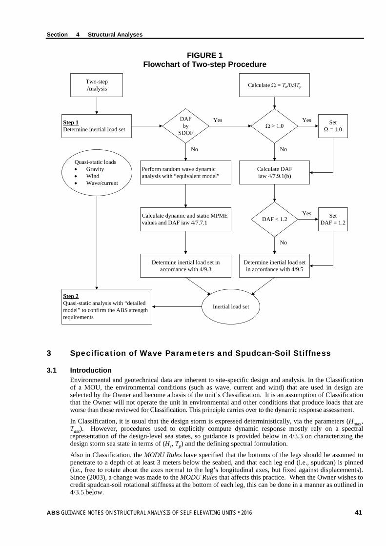
Section 4 Structural Analyses
FIGURE 1 Flowchart of Two-step Procedure
Two-step Analysis
Step 1Determine inertial load set
DAF by
SDOF
Perform random wave dynamic analysis with “equivalent model”
Calculate DAF iaw 4/7.9.1(b)
Ω > 1.0 SetΩ = 1.0
Calculate Ω = Tn/0.9Tp
Calculate dynamic and static MPME values and DAF iaw 4/7.7.1 DAF < 1.2 Set
DAF = 1.2
Determine inertial load set in accordance with 4/9.5
Determine inertial load set in accordance with 4/9.3
Quasi-static loads• Gravity• Wind• Wave/current
Step 2Quasi-static analysis with “detailed model” to confirm the ABS strength requirements
Inertial load set
Yes Yes
Yes
No No
No
3 Specification of Wave Parameters and Spudcan-Soil Stiffness
3.1 Introduction Environmental and geotechnical data are inherent to site-specific design and analysis. In the Classification of a MOU, the environmental conditions (such as wave, current and wind) that are used in design are selected by the Owner and become a basis of the unit’s Classification. It is an assumption of Classification that the Owner will not operate the unit in environmental and other conditions that produce loads that are worse than those reviewed for Classification. This principle carries over to the dynamic response assessment.
In Classification, it is usual that the design storm is expressed deterministically, via the parameters (Hmax, Tass). However, procedures used to explicitly compute dynamic response mostly rely on a spectral representation of the design-level sea states, so guidance is provided below in 4/3.3 on characterizing the design storm sea state in terms of (Hs, Tp) and the defining spectral formulation.
Also in Classification, the MODU Rules have specified that the bottoms of the legs should be assumed to penetrate to a depth of at least 3 meters below the seabed, and that each leg end (i.e., spudcan) is pinned (i.e., free to rotate about the axes normal to the leg’s longitudinal axes, but fixed against displacements). Since (2003), a change was made to the MODU Rules that affects this practice. When the Owner wishes to credit spudcan-soil rotational stiffness at the bottom of each leg, this can be done in a manner as outlined in 4/3.5 below.
ABS GUIDANCE NOTES ON STRUCTURAL ANALYSIS OF SELF-ELEVATING UNITS . 2016 41

Section 4 Structural Analyses
3.3 Spectral Characterization of Wave Data for Dynamic Analysis The wave conditions typically specified for Classification are regular waves. The deterministic parameters (Hmax, Tass) of the regular wave need to be restated as wave spectral parameters (Hs, Tp) for the dynamic analysis.
Where suitable data are not available, the following procedures may be used to convert the deterministic wave parameters to spectral parameters:
Hsrp = Hmax/1.75 (for cyclonic areas)
= Hmax/1.86 (for non-cyclonic areas) ........................................................................... (4.1)
Hs = [1.0 + (10Hsrp /Tp2) e(-d/25)] × Hsrp ........................................................................................ (4.2)
Tp = 1.05Tass when 4.00 srpH < Tp < 4.72 srpH
but if Tp > 4.72 srpH , then use Tp = 4.72 srpH
if Tp < 4.00 srpH , then use Tp = 4.00 srpH
where
Hsrp = significant wave height, in meters, of the three-hour storm for the assessment return period
Hs = effective significant wave height, in meters
d = water depth, in meters (d > 25 m)
Tp = peak period associated with Hsrp (also used with Hs), in seconds
Equation (4.2) is the Wheeler stretching, adjustment that accounts some nonlinear effects around the free surface in shallower water depth. The JONSWAP spectrum with a peak enhancement factor of 3.3 and the above calculated Hs and Tp should be used to represent the considered sea state. The short-crestedness of waves should not be considered.
3.5 Spudcan-Soil Rotational Stiffness (SC-S RS) The maximum extent to which this rotational stiffness can be applied to the system, Krs,fixed, is defined by the following equation.
Krs,fixed = E I /(L Cmin)
where
E = Young’s modulus, 209 GPa for steel
I = moment of inertia, in m4
L = sum of the distance, in m, from the underside of the hull to seabed plus the seabed penetration (minimum 3 meters) ≥ 4.35(I/As)0.5
Cmin = (1.5 – J)/(J + F)
J = 1 + [7.8 I/(As L2)]
F = 12 I Fg/(A Y2)
A = axial area of the equivalent leg, in m2
As = shear area of the leg, in m2
42 ABS GUIDANCE NOTES ON STRUCTURAL ANALYSIS OF SELF-ELEVATING UNITS . 2016
Section 4 Structural Analyses
Y = distance, in m, between the centerline of one leg and a line joining the centers of the other two legs for a 3-leg unit; the distance, in m, between the centers of leeward and windward rows of legs; in the direction of being considered
Fg = 1.125 for a three leg unit and 1.0 for a four leg unit
The Owner may select values of SC-S RS ranging from zero (the pinned ended condition) up to the maximum value indicated.
5 Dynamic Analysis Modeling
5.1 Introduction To determine a DAF, a simplified Dynamic Analysis model, as indicated below, may be used. The usual level of modeling employed in this case is designated as an “equivalent model”. Inaccurate or inappropriate modeling can have a major effect on the calculated structural responses, therefore, special care should be exercised to assure that the modeling and application of the dynamic loading is done appropriately. The stiffness of the Dynamic Analysis model should also be consistent with that of the “detailed” model used for the Quasi-Static structural analysis to check the adequacy of the structure by the permissible stress unity check criteria of the MODU Rules.
5.3 Stiffness Modeling The level of stiffness modeling of the “equivalent model” for dynamic analysis discussed in this section includes
• Leg stiffness
• Hull stiffness
• Leg-to-hull connection stiffness (stiffness of jacking system, proper load transfer direction of guides, pinions and clamps, etc.)
• P-Delta effect
• Foundation stiffness (leg-to-seabed interactions)
5.3.1 Leg Stiffness The stiffness of a leg is characterized by the following equivalent cross sectional properties:
• Cross sectional area
• Moment of inertia
• Shear area
• Torsional moment of inertia
The dominant factor affecting the leg stiffness is leg bending, but other compliance should be incorporated, such as the shear deflection of legs. The shear deflection of most members is small, but it can be significant in a ‘lattice’ structure. Therefore, shear deflection of legs should be properly incorporated in the analysis model.
In an equivalent model, a leg can be modeled by a series of collinear beams. The cross sectional properties of the beams may be derived by employing the formulas given in Subsection A1/3 or by applying various unit load cases to the detailed leg model, following the procedure given in 3/3.5.2. If the properties are calculated with the formulas, they may change along the axis of the leg because the properties of the members constituting the leg may vary along the axis of the leg. Although it is not required to model each bay of the leg with a beam element, doing this will facilitate a more accurate mass distribution along the leg.
A spudcan may usually be modeled as a rigid member.
ABS GUIDANCE NOTES ON STRUCTURAL ANALYSIS OF SELF-ELEVATING UNITS . 2016 43
Section 4 Structural Analyses
5.3.2 Hull Stiffness Hull structure can be modeled as a grillage of beam members. The properties of the beam may be calculated based on the depth of the bulkheads and side shell and the effective width of deck and bottom plating.
The overall structural stiffness or, in turn, the natural period of a unit is less sensitive to hull stiffness. Therefore, the grillage of beams can simply consist of several beam members at each location of the bulkheads and side shell. When considering the contribution from deck(s) and bottom plating, the effective width of deck(s) or bottom plating assigned to a beam member is so determined that the overlapping plan area reaches minimum, i.e., to minimize the areas whose contribution is either not included or included twice. This overlapping will happen when the axes of adjacent beams are not parallel to each other.
The second moment of area of the hull is normally much higher than that of the leg. A common error is to not make the rotational stiffness and “in plane” bending stiffness of equivalent hull members high enough.
5.3.3 Leg-to-Hull Connection Stiffness The leg-to-hull connection is very important to the dynamic analysis. The compliance of the connection is due to a number of factors:
• There may be a global rotation of the leg between the guides due to compliance of the jacking/holding system.
• There may be a global rotation of the leg between the guides due to the local deflection of the guide structure.
• Local deflection of the leg chords, induced by the guide reactions, may lead to an effective rotation of the leg. Also, deformation of the chord wall itself will produce additional leg rotation.
Due to this compliance of the connection, the rotational, horizontal and vertical stiffness of the connection should be modeled with adequate accuracy. A rigid connection is usually not considered acceptable unless the justification of this simplification is provided.
In an equivalent model, the rotational stiffness of the connection may be represented by linear rotational springs and the horizontal and vertical stiffness by linear translational springs. The stiffness of the springs may be derived by employing the formulas given in Subsection A2/3 or by applying various unit load cases to the detailed leg-to-hull connection model, provided the detailed model appropriately represents the stiffness of the connection, following the procedures given in Subsection A2/5.
5.3.4 P-Delta Effect – (P-∆) The actual structure will be less stiff than estimated from a linear analysis because of displacement dependent effects, P-∆ or Euler amplification. This will tend to increase the deflection of the structure, thereby reducing its effective stiffness. Therefore, the P-∆ effect should be accounted for in the Dynamic Analysis model.
As mentioned in Subsection 2/9, a common way to account for the P-∆ effect is the geometric stiffness method. In this method, negative stiffness correction terms are introduced into the global stiffness matrix of the Dynamic Analysis model. In order to do this, springs of negative stiffness are connected between each spring’s fixed reaction point and a point on each leg where the hull intersects the leg. The negative stiffness for horizontal displacements is given by:
Kpd = –Pg/L
where
Pg = total effective gravity load on each leg, including hull weight and weight of the leg above the hull and leg joint point
L = distance from the spudcan reaction point to the hull vertical center of gravity
44 ABS GUIDANCE NOTES ON STRUCTURAL ANALYSIS OF SELF-ELEVATING UNITS . 2016
Section 4 Structural Analyses
5.3.5 Foundation Stiffness Additional stiffness to represent the Spudcan-Soil Rotational Stiffness may be included in the model to the extent indicated in 4/3.5.
One way to implement this in the equivalent model is for each leg to have a pair of orthogonal rotational springs of specified stiffness horizontally connected to the reaction point on the leg and an “earth” point where all degrees of freedom are fixed.
5.5 Modeling the Mass The mass that will be dynamically excited and the distribution of that mass should be represented accurately in the Dynamic Analysis model. Items that should be considered include:
• The elevated mass (arising from hull self-weight; mass of additional equipment, variable mass from drilling equipment and consumables and other supplies)
• Leg mass, added mass and any entrained and entrapped (water) mass
• Spudcan mass and entrapped (water) mass
Usually, no mass from functional loads will need to be considered as participating in the dynamic response.
Leg mass can be modeled as nodal masses along the leg. A mass for each bay is adequate for the dynamic analysis. Added mass and any entrained/entrapped mass should be included. If more accurate information about mass distribution is not available, elevated weight may be modeled as nodal masses acting on the hull at its connection to legs.
5.7 Hydrodynamic Loading The hydrodynamic loads to be considered in the dynamic analysis are those induced by waves and waves acting with current. The basis of the hydrodynamic loading is Morison’s equation, as applied to the Dynamic Analysis model. Equivalent drag and mass coefficients should be developed for the “equivalent leg” idealization of the leg, and as applicable, the spudcan, etc. Formulas for deriving the equivalent drag and mass coefficients of the leg are presented in 2/7.3.4. The current profile should be as specified for Classification, with stretching and compression effects as specified in 1/5.5.3. The hydrodynamic load calculation should consider the relative velocities between the wave and the structure.
When deriving the hydrodynamic properties, such as equivalent diameter, area, drag and mass coefficients of a leg, it is important to account for all members, such as chords, horizontal members, diagonal members, span breakers, etc., in a bay of the leg and their orientations. Some of the properties, i.e., drag coefficient, are storm-heading-dependent.
Where the dynamic analysis is performed considering sea state simulation using random wave generation procedures, as described in Subsection 4/7, Airy wave theory can be used to develop the hydrodynamic forces.
When determining loads due to the simultaneous occurrence of waves and current using Morison’s equation, the current velocity is to be added vectorially to the wave particle velocity before the total force is computed.
5.9 Damping Damping can have a significant effect on the response. The total damping ratio to be used in the dynamic response analysis (expressed as a percentage of the critical damping) is defined as:
ζ = c/ccr · 100 %
where
c = system damping
ccr = critical damping = km ⋅2
ABS GUIDANCE NOTES ON STRUCTURAL ANALYSIS OF SELF-ELEVATING UNITS . 2016 45
Section 4 Structural Analyses
m = effective mass of the system
k = effective stiffness of the system
The total damping ratio should not be taken more than 7%. The three main sources of damping are:
• Structural, including holding system, normally taken as 2% maximum on an independent leg SEU.
• Small strain foundation, normally taken as 2% maximum for an SEU with independent legs.
• Hydrodynamic, if the relative velocity term is incorporated into the dynamic analysis, damping to account for hydrodynamic damping should not be considered. However, when using the approach that does not consider the relative velocity term, a maximum additional hydrodynamic damping of 3 % can be assumed.
7 Dynamic Response Analysis Methods
7.1 General An SEU responds dynamically to waves. This behavior should be modeled appropriately in the SEU’s global strength analysis by including the static and dynamic contributions. Fully detailed random wave dynamic analysis in the time domain may be pursued to obtain the static and dynamic responses for design of an SEU’s global strength. However, the “inertial load set” approach described in 4/1.3 is most often used in practical design, and yields sufficiently good results in normal circumstances. In this approach, the random wave dynamic analysis is performed only for determining appropriate values for DAFs and for subsequently capturing the dynamic contributions as inertial loads using the determined DAFs.
The random wave dynamic analysis approach is based on considering the wave (sea-state) as a random quantity. Using a time domain approach, the most probable maximum extreme (MPME) values of selected static and dynamic responses are obtained. The DAF is the ratio of the MPME of the dynamic response to that of the static response. The MPME is the mode, or highest point, of the probability density function (PDF) for the extreme of the response being considered. This is a value with an approximately 63% chance of exceedance, corresponding to the 1/1000 highest peak level in a sea-state with a 3-hour duration. There are several methods to predict a selected extreme response as will be addressed later in 4/7.3.
A simpler method referred to as the Single Degree of Freedom (SDOF) Approach can also be used for deriving the DAFs, which will be discussed later in 4/7.5. Due to the limitations of the single-degree-of-freedom (SDOF) approach the random-wave-time-domain approach is the preferred one to be applied for deriving the DAFs.
7.3 Random Wave Dynamic Analysis in Time Domain 7.3.1 General
The “equivalent” model indicated in Section 3 is usually employed in time domain analysis. In time domain simulation, a Gaussian random sea state is generated, and the time-step for the simulation is required to be sufficiently small. The duration of the simulation(s) should also be sufficiently long for the method being used to reliably determine the extreme values of the responses being sought.
The overall methodology is to determine the Most Probable Maximum Extreme (MPME) values of the dynamic and static responses in the time domain. The ratio of these two values – defined as DAF – represents the ratio by which the static response, obtained using a high order wave theory and the maximum wave height, should be increased in order to account for dynamic effects. A DAF can be calculated for each individual global response parameter (e.g., base shear, overturning moment or hull sway). Usually, DAF of overturning moment is higher than the other two.
46 ABS GUIDANCE NOTES ON STRUCTURAL ANALYSIS OF SELF-ELEVATING UNITS . 2016
Section 4 Structural Analyses
7.3.2 Random Wave Generation The wave elevation may be modeled as a linear random superposition of regular wave components, using information from the wave spectrum. The statistics of the underlying random process are Gaussian and fully known theoretically. An empirical modification around the free surface may be needed to account for free surface effects (Wheeler stretching, Equation 4.2). The following criteria are to be satisfied for the generated random waves.
7.3.2(a) Wave Components. The random wave generation should use at least 200 wave components with divisions of equal wave energy. It is recommended that smaller energy divisions be used in high frequency regions of the spectrum, where the enforcement and cancellation frequencies are located.
7.3.2(b) Validity of Generated Sea State. The generated random sea state must be Gaussian and should be checked for validity, as follows:
• Correct mean wave elevation
• Standard deviation = (Hs/4) ± 1%
• –0.03 < skewness < 0.03
• 2.9 < kurtosis < 3.1
• Maximum crest elevation = (Hs/4) )ln(2 N (error within –5% to +7.5%),
where
N = number of wave cycles in the time series being qualified, N ≈ Simulation Duration/Tz
Tz = zero up-crossing period of the wave
7.3.2(c) Random Seed Effect. Depending on the method used to predict extreme responses and DAF, the random seed effect can be significant. Care should be taken to ensure that the predicted results are not affected by the selection of random seeds.
7.3.3 Calculation of Structural Response The structural response should be obtained using the Dynamic Analysis model discussed in Section 3. The analysis model (i.e., the equivalent model with proper loading and boundary conditions) is to be solved using a reliable solver having the capability to do time domain calculations and response statistics calculations. Special attention is to be paid to the topics listed below.
7.3.3(a) Validity of the Natural Periods of Equivalent Model. The natural periods of a structure are the most important indicators of the dynamic characteristics of the structure. If the computed natural periods are not reasonable, there must be something wrong with the established equivalent model, either its stiffness distribution or its mass distribution, or both. Therefore, the check of natural periods is an indispensable step in the dynamic analysis.
The natural periods of the established equivalent model can be found by solving the eigen-value problem, and the fundamental natural period should be checked against that estimated from the SDOF approach in 4/7.5.1. It should note that the P-∆ effect should be accounted for in the Dynamic Analysis model as mentioned in 4/5.3.4.
7.3.3(b) Number of Simulations and Simulation Duration. There are four prevalent methods, as listed in 4/7.3.4, which can be used to establish the needed MPME values of the response from the time domain analysis. Each of these extreme value prediction methods has specific needs regarding the recommended number and duration of the simulations that should be performed to establish a sufficient statistical basis on which to obtain the MPME value. Therefore, the recommended number and duration of the simulations given below should be followed in the calculation of structural response.
ABS GUIDANCE NOTES ON STRUCTURAL ANALYSIS OF SELF-ELEVATING UNITS . 2016 47

Section 4 Structural Analyses
i) Drag-Inertia Parameter Method: Simulation time of at least 60 minutes; four simulations with different control parameters, i.e., fully dynamic, quasi-static, quasi-static with Cd (drag coefficient) = 0 and quasi-static with CMe (inertia coefficient) = 0.
ii) Weibull Fitting method: Simulation time of at least 60 minutes; number of simulation ≥ 5.
iii) Gumbel Fitting method: Simulation time of at least 180 minutes; number of simulation ≥ 10.
iv) Winterstein/Jensen method: Simulation time of at least 180 minutes; number of simulation = 1.
More detailed descriptions of these four methods are provided in 4/7.3.4.
It should be noted that the “static response analysis” described here and in 4/7.3.4(a) is performed using the Dynamic Analysis model, but with the mass and damping terms set to zero. This analysis is performed to establish DAFs. It should not be confused with the analysis that is described later with the more detailed model that is used for a Quasi-Static structural analysis to obtain the “unity-checks”, as described in Subsection 4/9.
7.3.3(c) Time Step of the Simulations. The integration time-step should be less than, or equal to, the smaller of the following equations, unless it can be shown that a larger time-step leads to no significant change in results.
Tz/20 or Tn/20
where
Tz = zero up-crossing period of the wave
= Tp/1.406 for the Pierson-Moskowitz spectrum
Tn = first mode natural period of the SEU
7.3.3(d) Transients. Transient response is to be discarded by removing the first 100 seconds of the response time series before predicting the extreme responses.
7.3.3(e) Relative Velocity. It is expected that the relative velocity between the wave particle and structural velocities will be included in the hydrodynamic force formulations used in the time domain analysis. (See also 2/7.13)
7.3.4 Prediction of Extreme Responses Although the waves are considered linear and statistically Gaussian, the structural response of an SEU is likely to be non-Gaussian due to non-linear drag force and free surface effects which are included in the wave kinematics calculations. The statistics of such a non-Gaussian process are generally not known theoretically, but the extremes are generally larger than the extremes of a corresponding Gaussian random process. For a detailed investigation of the dynamic behavior of an SEU, the non-Gaussian effects should be included. The four prevalent methods elaborated below are considered acceptable for this purpose.
7.3.4(a) Method I – Drag/Inertia Parameter Method. The drag/inertia parameter method is based on the assumption that the extreme value of a standardized process can be calculated by splitting the process into two parts, evaluating the extreme values of each and the correlation coefficient between the two, then combining as:
(mpmR)2 = (mpmR1)2 + (mpmR2)
2 + 2ρR12(mpmR1)(mpmR2) ............................................. (4.3)
The extreme values of the dynamic response can therefore be estimated from the extreme values of the static response, which is obtained by solving the dynamic equation with both mass term and damping term equal to zero, and the so-called “inertia” response, which is in fact the difference between the dynamic response and the static response. The correlation coefficient of the static and “inertia” responses is calculated as:
48 ABS GUIDANCE NOTES ON STRUCTURAL ANALYSIS OF SELF-ELEVATING UNITS . 2016
Section 4 Structural Analyses
RiRs
RiRsRdR σσ
σσσρ2
222 −−= .................................................................................................. (4.4)
The extreme value of the “inertia” response can be reasonably expressed as:
mpmRi = 3.7 σRi .............................................................................................................. (4.5)
In the drag/inertia method the extreme value used is the MPME value of the response and the method requires the response of the SEU to be determined for four conditions. In all four cases the storm simulation (random seed) should be identical, but with different components of the loading and/or response simulated. The responses considered will usually be total wave and current base shear and total wave and current overturning moment, for computing the base shear and overturning moment DAFs, respectively.
The four cases to be simulated are full dynamic response, full static response, static response to inertia only wave loading (setting Cd = 0) and static response to drag only loading (setting Cm = 0). From these the inertial response is obtained as the full dynamic response minus the full static response. The means and standard deviations of the response are extracted from the time domain responses and the DAFs computed as illustrated in Section 4, Figure 2.
The drag-inertia method given here includes a final step to scale the DAF based on the period ratio Tn/Tp. This step is included to ensure that the DAF values are not underestimated for cases where Tn approaches Tp, see Reference 7. The equation for the scaling factor is given in Section 4, Figure 2, and it is illustrated in Section 4, Figure 3.
ABS GUIDANCE NOTES ON STRUCTURAL ANALYSIS OF SELF-ELEVATING UNITS . 2016 49
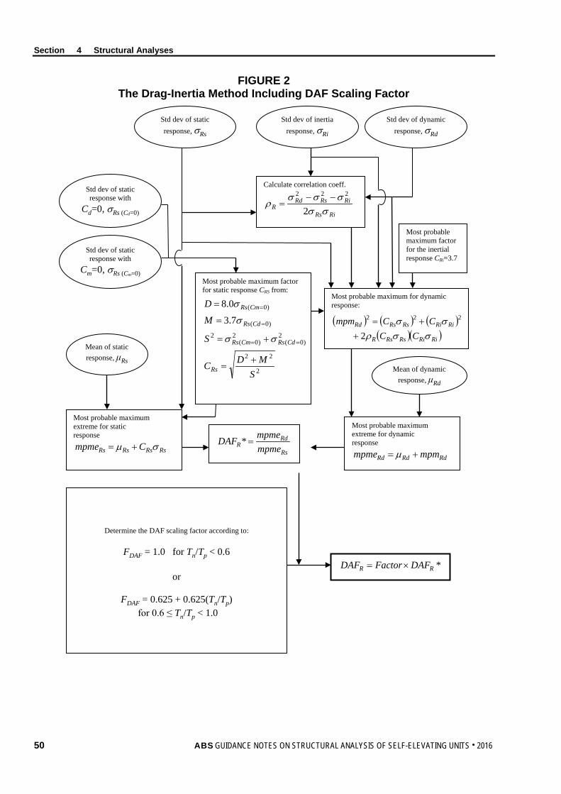
Section 4 Structural Analyses
FIGURE 2 The Drag-Inertia Method Including DAF Scaling Factor
Mean of static response, μRs
Mean of dynamic response, μRd
Std dev of dynamic response, σRd
Std dev of static response, σRs
Std dev of inertia response, σRi
Calculate correlation coeff.
RiRs
RiRsRdR σσ
σσσρ
2
222 −−=
Std dev of static response with
Cd=0, σRs (Cd=0)
Std dev of static response with
Cm=0, σRs (Cm=0) Most probable maximum factor for static response CRS from:
2
22
2)0(
2)0(
2
)0(
)0(
7.3
0.8
SMDC
S
M
D
Rs
CdRsCmRs
CdRs
CmRs
+=
+=
=
=
==
=
=
σσ
σ
σ
Most probable maximum factor for the inertial response CRi=3.7
Most probable maximum extreme for static response
RsRsRsRs Cmpme σµ +=
Most probable maximum for dynamic response:
( ) ( ) ( )( )( )RiRiRsRsR
RiRiRsRsRd
CCCCmpm
σσρσσ
2
222
++=
Most probable maximum extreme for dynamic response
RdRdRd mpmmpme += µ
Rs
RdR mpme
mpmeDAF =*
*RR DAFFactorDAF ×=
Determine the DAF scaling factor according to:
FDAF = 1.0 for Tn/Tp < 0.6
or
FDAF = 0.625 + 0.625(Tn/Tp) for 0.6 ≤ Tn/Tp < 1.0
50 ABS GUIDANCE NOTES ON STRUCTURAL ANALYSIS OF SELF-ELEVATING UNITS . 2016
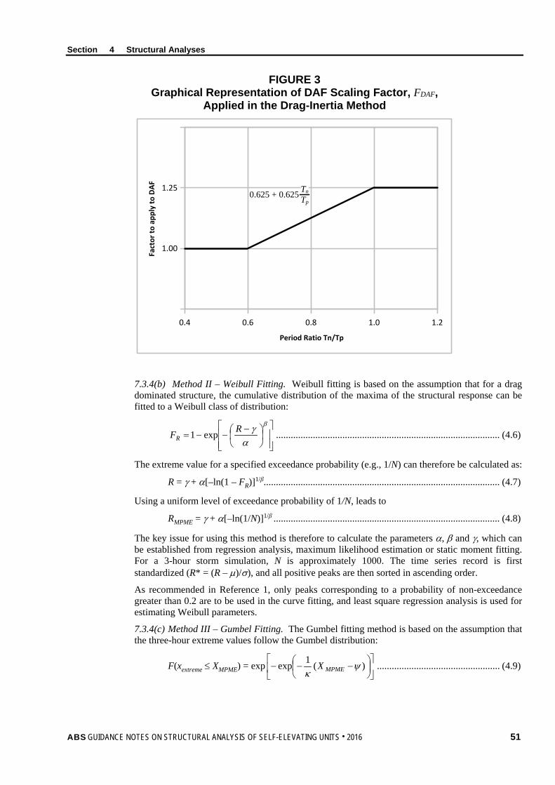
Section 4 Structural Analyses
FIGURE 3 Graphical Representation of DAF Scaling Factor, FDAF,
Applied in the Drag-Inertia Method
0.4 0.6 0.8 1.0 1.2
1.00
1.25
Period Ratio Tn/Tp
Fact
or to
app
ly to
DAF
0.625 + 0.625 TnTp
7.3.4(b) Method II – Weibull Fitting. Weibull fitting is based on the assumption that for a drag dominated structure, the cumulative distribution of the maxima of the structural response can be fitted to a Weibull class of distribution:
−
−−=β
αγRFR exp1 ........................................................................................... (4.6)
The extreme value for a specified exceedance probability (e.g., 1/N) can therefore be calculated as:
R = γ + α[–ln(1 – FR)]1/β................................................................................................ (4.7)
Using a uniform level of exceedance probability of 1/N, leads to
RMPME = γ + α[–ln(1/N)]1/β ............................................................................................ (4.8)
The key issue for using this method is therefore to calculate the parameters α, β and γ, which can be established from regression analysis, maximum likelihood estimation or static moment fitting. For a 3-hour storm simulation, N is approximately 1000. The time series record is first standardized (R* = (R – µ)/σ), and all positive peaks are then sorted in ascending order.
As recommended in Reference 1, only peaks corresponding to a probability of non-exceedance greater than 0.2 are to be used in the curve fitting, and least square regression analysis is used for estimating Weibull parameters.
7.3.4(c) Method III – Gumbel Fitting. The Gumbel fitting method is based on the assumption that the three-hour extreme values follow the Gumbel distribution:
F(xextreme ≤ XMPME) = exp
−−− )(1exp ψ
κ MPMEX .................................................. (4.9)
ABS GUIDANCE NOTES ON STRUCTURAL ANALYSIS OF SELF-ELEVATING UNITS . 2016 51
Section 4 Structural Analyses
The most probable maximum extreme discussed here corresponds to an exceedance probability of 1/1000 in a distribution function of individual peaks or to 0.63 in an extreme probability distribution function. The MPME of the response can therefore be calculated as:
XMPME = ψ –κ ln–ln[F(XMPME)]
= ψ – κ ln[–ln(0.37)] ≈ ψ ............................................................................... (4.10)
Now, the key issue is to estimate the parameters ψ and κ based on the response obtained from time-domain simulations. Reference 1 recommends that the maximum simulated value be extracted for each of the ten 3-hour response simulations, and that the parameters be computed by maximum likelihood estimation. Similar calculations should also be performed using the ten 3-hour minimum values. Although it is always possible to apply the maximum likelihood fit numerically, the method of moments may be preferred. See Reference 8.
For the Gumbel distribution, the mean and variance are given by:
Mean: μ = ψ + γ⋅κ, γ = Euler constant (0.5772…)
Variance: σ2 = π2κ2 / 6
By which means, the parameters ψ and κ can be directly obtained using the moment fitting method:
κ = π
σ6 , ψ = μ – 0.57722κ .................................................................................... (4.11)
7.3.4(d) Method IV – Winterstein/Jensen Method. The basic premise of Winterstein/Jensen method is that a non-Gaussian process can be expressed as a polynomial (e.g., a power series or an orthogonal polynomial) of a zero mean, narrow-banded Gaussian process (represented here by the symbol U), that is
R(U) = C0 + C1U + C2U2 +C3U
3 .................................................................................. (4.12)
The same relationship exists between the MPMEs of the two processes. Since the MPME of Gaussian process U is theoretically known, the MPME of the non-Gaussian process can be calculated if the coefficients C0, C1, C2, C3 are determined.
i) Determination of Um. Calculate the following statistical quantities of the time series for the response parameter R under consideration:
µR = mean of the process
σR = standard deviation
α3 = skewness
α4 = kurtosis
Then construct a standardized response process, z = (R − µR)/σR. Using this standardized process, calculate the number of zero-upcrossings, N. In lieu of an actual cycle count from the simulated time series, N = 1000 may be assumed for a 3-hour simulation.
The most probable value, Um, of the transformed process is computed by the following equation:
Um = ( )
⋅
hoursintimesimulationhours3log2 Ne ........................................................... (4.13)
where Um is the most probable value of a Gaussian process of zero mean, unit variance.
52 ABS GUIDANCE NOTES ON STRUCTURAL ANALYSIS OF SELF-ELEVATING UNITS . 2016
Section 4 Structural Analyses
ii) Determination of C coefficients. One can establish the following equations for C1, C2 and C3:
σR2 = C1
2 + 6C1C3 + 2C22 + 15C3
2
σR3α3 = C2(6C1
2 + 8C22 + 72C1C3 + 270C3
2)
σR4α4 = 60C2
4 + 3C14 + 10395C3
4 + 60C12C2
2 + 4500C22C3
2 + 630C12C3
2 + 936C1C2
2C3 + 3780C1C33 + 60C1
3C3
Solve the equations with the initial guesses as:
C1 = σRK(1 – 3h4)
C2 = σRKh3
C3 = σRKh4
where
h3 = α3/ [ ])3(5.1124 4 −++ α
h4 = [ ]1)3(5.11 4 −−+ α /18
K = [1 + 2h32 + 6h4
2]-1/2
Obtain
C0 = µR – σRKh3
iii) Determination of RMPME. The most probable maximum extreme in a 3-hour storm, for the response under consideration, can be computed from the following equation:
RMPME = C0 + C1Um1 + C2Um
2 + C3Um3 ......................................................... (4.14)
7.5 Other Dynamic Analysis Methods The random wave time domain method is the recommended approach for the dynamic analysis of an SEU. However, the analysis procedure is relatively complicated and under some circumstances, other methods can also generate results of sufficient accuracy. Besides, some results obtained from the simpler methods, (e.g., natural period of the structure determined by SDOF approach) can be used to check the results of time domain analysis. For these reasons, the single degree of freedom approach is briefly discussed below. A frequency domain analysis method may be useful for limited preliminary or comparative studies of system responses. However a frequency domain analysis method is not recommended as the final basis of design.
7.5.1 Single-Degree-of-Freedom Approach In a single-degree-of-freedom (SDOF) approach, the SEU is modeled as a simple mass/spring/ damper system. Due to its simplicity, this approach is recommended for an initial evaluation of the dynamic amplification or for use with limitations given in 4/7.5.1(d).
7.5.1(a) Natural Period. The natural period of an SEU is an important indicator of the degree of dynamic response to be expected. The first and second vibratory modes are usually surge and sway (i.e., lateral displacements at the deck level). The natural periods of these two modes are usually close to each other. Which of the two is higher depends on which direction of the structure is less stiff. The third vibratory mode is normally a torsional mode. Since the period varies with the environmental load direction, care should be taken that the period used in analysis is consistent with the environmental load being considered.
An estimate of the first mode (fundamental) natural period, Tn, is obtained for a single-degree-of-freedom (SDOF) system, as follows:
ABS GUIDANCE NOTES ON STRUCTURAL ANALYSIS OF SELF-ELEVATING UNITS . 2016 53
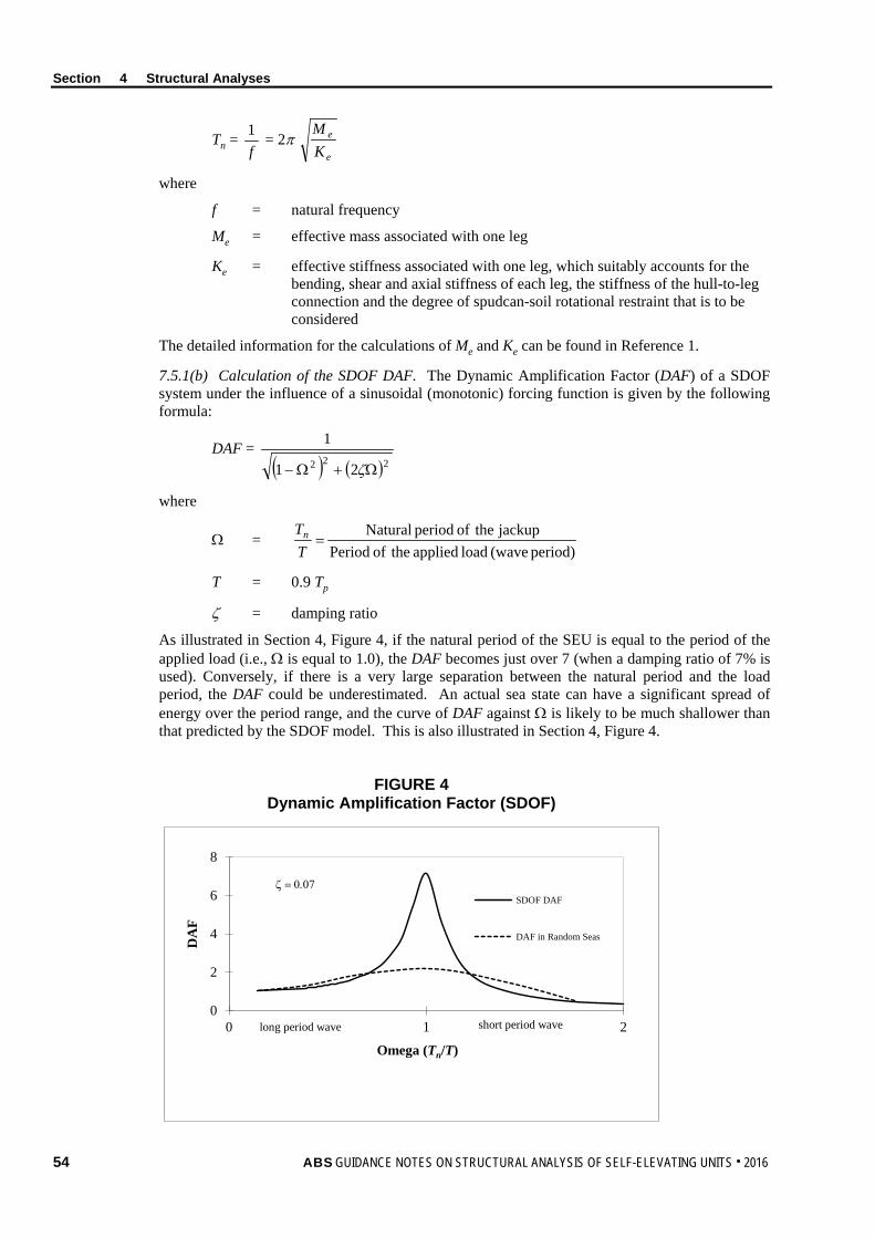
Section 4 Structural Analyses
Tn = f1 = 2π
e
e
KM
where
f = natural frequency
Me = effective mass associated with one leg
Ke = effective stiffness associated with one leg, which suitably accounts for the bending, shear and axial stiffness of each leg, the stiffness of the hull-to-leg connection and the degree of spudcan-soil rotational restraint that is to be considered
The detailed information for the calculations of Me and Ke can be found in Reference 1.
7.5.1(b) Calculation of the SDOF DAF. The Dynamic Amplification Factor (DAF) of a SDOF system under the influence of a sinusoidal (monotonic) forcing function is given by the following formula:
DAF = ( ) ( )222 21
1
Ω+Ω− ζ
where
Ω = period) (wave load applied theof Period
jackup theof period Natural=
TTn
T = 0.9 Tp
ζ = damping ratio
As illustrated in Section 4, Figure 4, if the natural period of the SEU is equal to the period of the applied load (i.e., Ω is equal to 1.0), the DAF becomes just over 7 (when a damping ratio of 7% is used). Conversely, if there is a very large separation between the natural period and the load period, the DAF could be underestimated. An actual sea state can have a significant spread of energy over the period range, and the curve of DAF against Ω is likely to be much shallower than that predicted by the SDOF model. This is also illustrated in Section 4, Figure 4.
FIGURE 4 Dynamic Amplification Factor (SDOF)
0
2
4
6
8
0 1 2
DA
F
Omega (Tn/T)
SDOF DAF
DAF in Random Seas
long period wave short period wave
ζ = 0.07
54 ABS GUIDANCE NOTES ON STRUCTURAL ANALYSIS OF SELF-ELEVATING UNITS . 2016
Section 4 Structural Analyses
Care should be taken when determining the appropriate wave period to be used in an SDOF analysis. A range of wave periods should be investigated, along with a range of associated wave heights. The applicable sea states that result in maximum responses should be identified and used in the assessment of the adequacy of the structure’s strength.
7.5.1(c) Dynamic Load Application. The dynamic effect can be applied to the Quasi-Static model by applying an extra force representing the dynamically-induced inertial load set at the center of gravity of the hull structure. The procedure is presented in Subsection 4/9.
7.5.1(d) Limitations. The greatest problems with the SDOF approach are that it may grossly over-estimate the response when the natural period of the unit is close to the monotonic period of the applied load and may possibly underestimate the response when there are large differences in periods or the natural period of the unit is longer than the period of the applied load (Ω > 1.0). However, this method can give reasonable results when Ω is in the range of 0.4 to 0.8 and the current velocity is small relative to the wave particle velocity. Therefore, the following limitations should apply:
i) The SDOF method can be unconservative for cases where the current velocity is large relative to the wave particle velocities. If the results of the analysis are close to the acceptance criteria further detailed analysis is recommended.
ii) The SDOF method can be unconservative and should not normally be used in an extreme storm analysis when Ω is greater than 1.0 (i.e., when Tn > 0,9Tp). However, the SDOF analogy may be used when the calculated Ω is greater than 1.0 providing Ω is taken as 1.0.
iii) A minimum value of 1.2 should be taken as the DAF for developing the inertial load set, regardless of the DAF calculated using the SDOF method.
9 Dynamic Amplification Factor and Inertial Load Set
9.1 Introduction The inertial load set required to perform a “two-step” analysis is calculated based on DAFs. The DAFs can be obtained from the random wave dynamic analysis or the SDOF approach. A commonly accepted way that the inertial load set is included in the “detailed” model for Quasi-Static structural analysis is as a concentrated load applied to the elevated hull structure. This idealization is most suitable for the case where the preponderance of the structural system’s total mass is in the hull, which is usually considered to be the case. If it were not the case, the complexity of the inertial load set would increase so that instead of a concentrated load, the inertial loads should be distributed in accordance with the mass distribution and vibratory mode shapes.
The inertial load sets calculated from the random wave dynamic analysis or the SDOF approach will not be the same, as is presented later in 4/9.3 and 4/9.5. Thus, when applying the inertial load set to the “detailed” model to simulate the dynamic response for a Quasi-Static structural analysis, special care should be exercised.
9.3 Inertial Load Set based on Random Wave Dynamic Analysis The random wave dynamic analysis usually generates the DAFs for Overturning Moment (OTM) and Base Shear (BS) force. Thus, the magnitude of the concentrated inertial load set representing the dynamic response from waves (or waves acting with current) in the wave loading direction can be obtained from the following quantities:
d = vertical distance from the base of a leg to a location in the elevated hull structure where the concentrated inertial load is to be imposed.
DAFOTM = dynamic amplification factor for overturning moment obtained from the Dynamic Response analysis using the MPME values for the dynamic and statically considered simulated hydrodynamic loads on the unit
DAFBS = dynamic amplification factor for the base shear force obtained from the Dynamic Response analysis using the MPME values for the dynamic and statically considered simulated hydrodynamic loads on the unit
ABS GUIDANCE NOTES ON STRUCTURAL ANALYSIS OF SELF-ELEVATING UNITS . 2016 55
Section 4 Structural Analyses
OTMQS = maximum, deterministic overturning moment from the considered wave (or wave acting with current) on the Quasi-Static structural model before the imposition of the inertial load set.
BSQS = maximum, deterministic shear force from the considered wave (or wave acting with current) on the Quasi-Static structural model before the imposition of the inertial load set.
The magnitude of the concentrated inertial force, FI, and the correction moment, OTMCorrection, are then found, respectively, from the following equations:
FI = (DAFBS – 1) BSQS
OTMCorrection = (DAFOTM – 1) OTMQS – FI d
Depending on the purpose of the analysis, the correction moment can be applied as
• Horizontal or vertical couple in the hull (although these may cause additional stress in the hull structure) if the primary concern of the analysis is for leg and foundation.
• Concentrated moment at the base of the leg (although this may cause inaccuracies in the foundation model for other than pinned conditions) if the primary concern of the analysis is for hull.
9.5 Inertial Load Set based on SDOF Approach When the SDOF approach presented in 4/7.5.1 is applied, the procedure that should be followed to establish the inertial load set is as follows.
The magnitude of the inertial load set is determined from:
Fi = (DAF − 1) × Fwave amp
where
Fi = inertial load set to be applied at the center of gravity of the hull
DAF = SDOF dynamic amplification factor
Fwave amp = static amplitude wave force = 0.5(Fmax − Fmin)
Fmax, Fmin = maximum/minimum total combined wave and current force (or wave/current base shear) obtained from quasi-static structural analysis, using the appropriate sea state
9.7 Inertial Load Set Applications The inertial load set is combined with all of the other statically considered loads, such as those from wind, currents, deterministically considered wave, weights, functional loads, etc. that should be included in the “detailed” model for a quasi-static structural analysis to obtain the stresses and deflections for evaluations with respect to the acceptance criteria given in the MODU Rules.
56 ABS GUIDANCE NOTES ON STRUCTURAL ANALYSIS OF SELF-ELEVATING UNITS . 2016
ABS GUIDANCE NOTES ON STRUCTURAL ANALYSIS OF SELF-ELEVATING UNITS . 2016 57
S e c t i o n 5 : C o m m e n t a r y o n A c c e p t a n c e C r i t e r i a
S E C T I O N 5 Commentary on Acceptance Criteria
1 Introduction The acceptance criteria for an SEU are specified in the MODU Rules. Some guidance on applying these criteria is given in this Section.
3 Categories of Criteria There are several categories of limiting criteria that need to be checked as follows.
Wave crest clearance and air gap
Overturning stability
Structural strength
Strength of the Elevating Machinery
While the criteria for these categories are checked separately by criteria given in the MODU Rules, it should be borne in mind that an individual limit in one category may influence another. The listed items can be called ultimate limit states, since the failure to satisfy the criteria will directly lead to serious damage, or even loss, of the unit. These limit states are within the scope of Classification, and will be discussed further below. The designer also needs to account for numerous other limit states both ultimate and serviceability related that are site-specific and are outside of the scope of Classification as a MODU; such as, foundation strength and stability, side-sway of the unit, etc. Criteria for the fatigue limit state of portions of the unit’s structure also need to be assessed.
5 Wave Crest Clearance and Air Gap A crest clearance of either 1.2 m (4 ft) or 10% of the combined storm tide, astronomical tide, and height of the maximum wave crest above the mean low water level, whichever is less, between the underside of the unit in the elevated position and the crest of the wave is to be maintained. This crest elevation is to be measured above the level of the combined astronomical tide and storm tides. Thus, the air gap, measuring from the still water line to the underside of the unit when elevated should be larger than the total elevation of the required crest clearance and the crest of the maximum anticipated wave.
7 Overturning Stability The overturning stability criterion has to be met in the unit’s elevated mode. For an independent leg SEU, the generally expression for stability checking can be expressed as:
E
LD
M
MM F.S. ....................................................................................................................... (5.1)
where
MD = stabilization moment from dead load
ML = stabilization moment from live load
ME = overturning moment from environmental load including inertial load
F.S. = factor of safety, 1.1 as per the MODU Rules
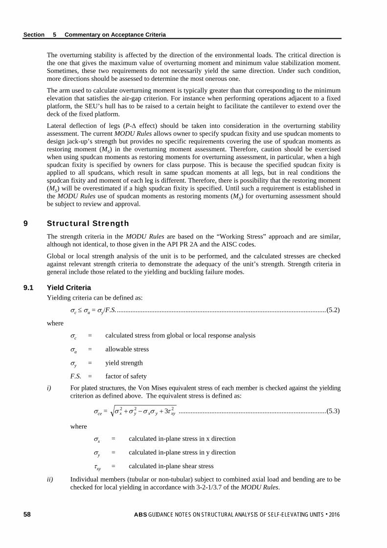
Section 5 Commentary on Acceptance Criteria
The overturning stability is affected by the direction of the environmental loads. The critical direction is the one that gives the maximum value of overturning moment and minimum value stabilization moment. Sometimes, these two requirements do not necessarily yield the same direction. Under such condition, more directions should be assessed to determine the most onerous one.
The arm used to calculate overturning moment is typically greater than that corresponding to the minimum elevation that satisfies the air-gap criterion. For instance when performing operations adjacent to a fixed platform, the SEU’s hull has to be raised to a certain height to facilitate the cantilever to extend over the deck of the fixed platform.
Lateral deflection of legs (P-∆ effect) should be taken into consideration in the overturning stability assessment. The current MODU Rules allows owner to specify spudcan fixity and use spudcan moments to design jack-up’s strength but provides no specific requirements covering the use of spudcan moments as restoring moment (MS) in the overturning moment assessment. Therefore, caution should be exercised when using spudcan moments as restoring moments for overturning assessment, in particular, when a high spudcan fixity is specified by owners for class purpose. This is because the specified spudcan fixity is applied to all spudcans, which result in same spudcan moments at all legs, but in real conditions the spudcan fixity and moment of each leg is different. Therefore, there is possibility that the restoring moment (MS) will be overestimated if a high spudcan fixity is specified. Until such a requirement is established in the MODU Rules use of spudcan moments as restoring moments (MS) for overturning assessment should be subject to review and approval.
9 Structural Strength The strength criteria in the MODU Rules are based on the “Working Stress” approach and are similar, although not identical, to those given in the API PR 2A and the AISC codes.
Global or local strength analysis of the unit is to be performed, and the calculated stresses are checked against relevant strength criteria to demonstrate the adequacy of the unit’s strength. Strength criteria in general include those related to the yielding and buckling failure modes.
9.1 Yield Criteria Yielding criteria can be defined as:
σc ≤ σa = σy/F.S. .......................................................................................................................... (5.2)
where
σc = calculated stress from global or local response analysis
σa = allowable stress
σy = yield strength
F.S. = factor of safety
i) For plated structures, the Von Mises equivalent stress of each member is checked against the yielding criterion as defined above. The equivalent stress is defined as:
σce = 222 3 xyyxyx τσσσσ +−+ ...................................................................................... (5.3)
where
σx = calculated in-plane stress in x direction
σy = calculated in-plane stress in y direction
τxy = calculated in-plane shear stress
ii) Individual members (tubular or non-tubular) subject to combined axial load and bending are to be checked for local yielding in accordance with 3-2-1/3.7 of the MODU Rules.
58 ABS GUIDANCE NOTES ON STRUCTURAL ANALYSIS OF SELF-ELEVATING UNITS . 2016
Section 5 Commentary on Acceptance Criteria
9.3 Buckling Criteria i) Individual members (tubular or non-tubular) subject to axial load and bending are to be checked
for beam column buckling in accordance with 3-2-1/3.7 and 3-2-1/3.9 of the MODU Rules.
ii) Plate and shell elements of the hull structure subject to compression load are to be checked against various buckling modes in accordance with the ABS Guide for the Buckling and Ultimate Strength Assessment for Offshore Structures.
9.5 Hybrid Members Members that are fabricated from materials of different yield strengths need to be carefully considered to ensure that the correct material properties are used. As a general rule, the unity checking for each different yield strength material should be done bearing in mind that the worst unity check may not occur at the section’s extreme fibers.
When calculating the buckling strength of a member under axial load only, one should use the lowest yield point for any material at the extreme fiber. When calculating the unity check for a member subject to both compression and bending, one should use the yield point of the material under consideration. This means that the Euler buckling load, eF ′ will have different values for a given cross section, depending on the material strength of the part that is being checked.
For the case of the triangular chord section as shown in Section 5, Figure 1, it should be noted that for strong axis bending the high stress would be at the extreme fiber of the rack; for weak axis bending the high stress would be at the extreme fiber of the back plate. Assume that the rack, side plates, and back plate are all of different yield strengths. The chord-buckling load, due to axial load only, would be based on the lower yield strength of either the rack or the back plate (assuming inelastic buckling). The yield strength of the side plates would not matter in most cases as they are unlikely to be close enough to the extreme fiber to suffer buckling induced inelastic yielding.
When assessing the chord for combined axial and bending stresses, it is necessary to check each point individually. These points would include:
• The extreme fiber of the rack. Note that the strong axis bending stresses will be high, but the orthogonal weak axis bending stress could be higher in the back plate.
• The extreme fiber of the back plate. Note that in strong axis bending, this will normally produce lower stresses than in the rack; but in the weak axis bending, the stress will be higher
• The juncture of the side plate to the rack
• The juncture of the side plate to the back plate
These points are plotted in Section 5, Figure 1.
ABS GUIDANCE NOTES ON STRUCTURAL ANALYSIS OF SELF-ELEVATING UNITS . 2016 59
Section 5 Commentary on Acceptance Criteria
FIGURE 1 Chords Section Stress Points
DC
BA
AB
CE
F
D Back Plate
Side Plate
Rack Plate
Rack Plate
Split Tubular
Opposed RackSplit Tubular
Chord Member SectionTriangular Type
Chord Member Section
In certain cases, it may be acceptable to use an average allowable bending stress for a hybrid member instead of using various yield strengths for different part of the member.
9.7 Punching Shear Punching shear is usually not an issue for leg design because the component members normally have relatively high wall thickness. Caution should, however, be taken is some special cases. The typical source of information on punching shear can be found in API RP 2A. This can be applied to most situations, including intelligent modification to account for a brace intersecting with a flat plate. Where standard parametric formulae cannot be found, it may be necessary to undertake a finite element analysis to determine the effectiveness of the joint design, especially one having a gusset plate.
9.9 P-∆ Effect on Member Checking An Euler modification, CM/(1 – fa/ exF ′ ), is specified by older AISC criteria (which is also referred to in API RP 2A) to account for the local P-∆ effects at member code checking under combined loading conditions. If the individual member loads come from a second order analysis (i.e., the equilibrium condition were formulated on the elastically deformed structure and local P-∆ load are also included in the analysis), the modification term CM/(1 – fa/ exF ′ ) needs to be set as unity.
The virtual negative springs are to account for the global P-∆ effect and have no impact on the member checking. Therefore the modification term CM/(1 – fa/ exF ′ ) is still applicable for such case.
11 Fatigue of Structural Details The fatigue criteria to be applied to the structural details of an SEU are given in the ABS Guide for the Fatigue Assessment of Offshore Structures.
13 Strength of the Elevating Machinery See Section 6-1-9 of the MODU Rules for design and certification criteria for the jacking system and holding mechanism of an SEU. The strength criteria for the structure supporting the elevating machinery are those given previously in Subsection 5/9. The load in the jacking system can be determined from the quasi-static analysis. Detailed model may be required for the comprehensive checking on specific load on each individual jacking gear.
60 ABS GUIDANCE NOTES ON STRUCTURAL ANALYSIS OF SELF-ELEVATING UNITS . 2016
Section 5 Commentary on Acceptance Criteria
15 Spudcan Check The spudcan structure and connection with the leg should have sufficient strength to resist the most severe load combinations (axial force, shear force and moment if applicable) expected.
The most severe load combinations acting on any spudcan under the following load conditions should be obtained from the global analysis; and the spudcan structures should be checked against these load combinations in accordance with the strength criteria given previously in Subsection 5/9.
15.1 Preload Condition The maximum required preload, concentrically distributed over a range of bearing areas, from the minimum design penetration up to and including full embedment.
15.3 Normal Operating and Severe Storm Conditions 15.3.1 Pin-ended Support
The maximum vertical reaction and the associated horizontal reaction in conjunction with 35% of the maximum calculated moment at the lower guide, (to account for the eccentric effects of possible scour and uneven bottom conditions) acting in the most unfavorable direction. The maximum lower guide bending moment is to be calculated with pin-ended conditions.
15.3.2 Partially-fixed Support i) The maximum vertical reaction, in conjunction with the associated horizontal reaction
and spudcan-soil fixity moment, acting in the most unfavorable direction.
ii) The maximum spudcan-soil fixity moment in conjunction with the associated vertical and horizontal reactions, acting in the most unfavorable direction.
17 Other Checks The foundation (soil’s) assessment does not have to be investigated for Classification. This is a site-specific issue under the control of the Owner.
Horizontal sway and other displacement limits, while not directly in the scope of Classification of a unit, may affect the Classification of drilling equipment and the ABS certification of other equipment. Checks that these limits will not be exceeded can usually be accomplished in a straightforward manner based on structural analysis result.
ABS GUIDANCE NOTES ON STRUCTURAL ANALYSIS OF SELF-ELEVATING UNITS . 2016 61
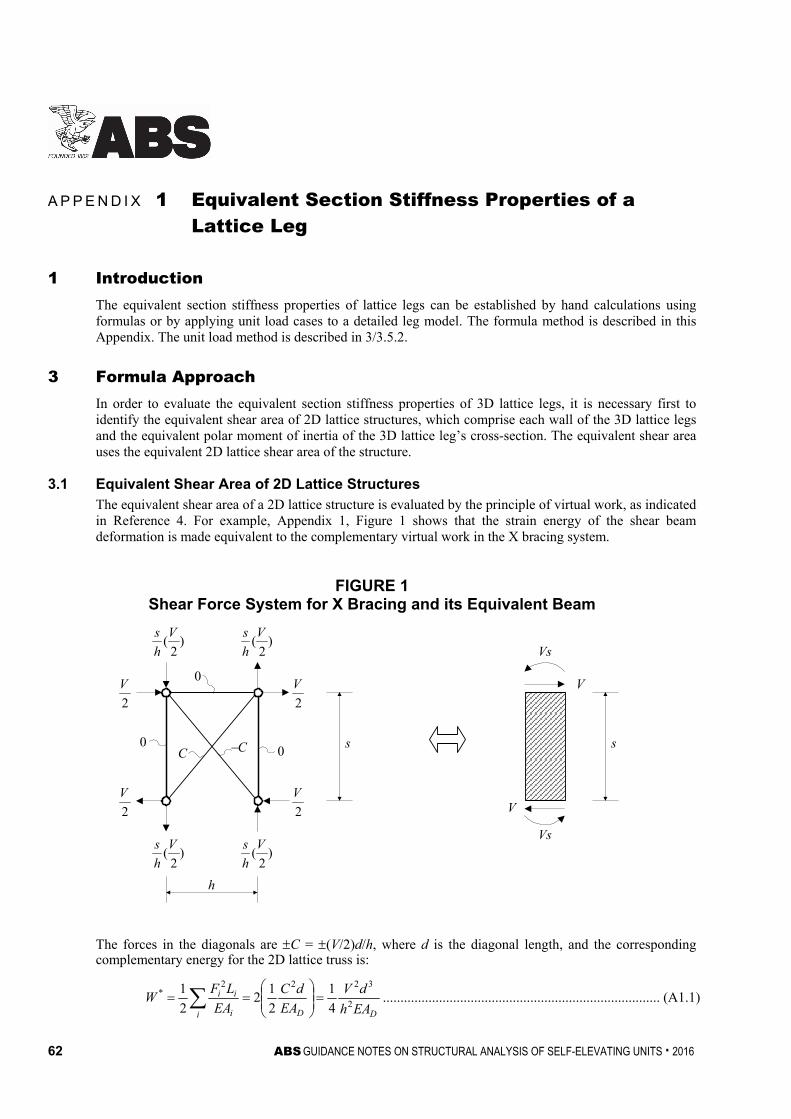
62 ABS GUIDANCE NOTES ON STRUCTURAL ANALYSIS OF SELF-ELEVATING UNITS . 2016
A p p e n d i x 1 : E q u i v a l e n t S e c t i o n S t i f f n e s s P r o p e r t i e s o f a L a t t i c e L e g
A P P E N D I X 1 Equivalent Section Stiffness Properties of a Lattice Leg
1 Introduction The equivalent section stiffness properties of lattice legs can be established by hand calculations using formulas or by applying unit load cases to a detailed leg model. The formula method is described in this Appendix. The unit load method is described in 3/3.5.2.
3 Formula Approach In order to evaluate the equivalent section stiffness properties of 3D lattice legs, it is necessary first to identify the equivalent shear area of 2D lattice structures, which comprise each wall of the 3D lattice legs and the equivalent polar moment of inertia of the 3D lattice leg’s cross-section. The equivalent shear area uses the equivalent 2D lattice shear area of the structure.
3.1 Equivalent Shear Area of 2D Lattice Structures The equivalent shear area of a 2D lattice structure is evaluated by the principle of virtual work, as indicated in Reference 4. For example, Appendix 1, Figure 1 shows that the strain energy of the shear beam deformation is made equivalent to the complementary virtual work in the X bracing system.
FIGURE 1 Shear Force System for X Bracing and its Equivalent Beam
0
)2
(V
h
s)
2(V
h
s
00
2
V
2
V
2
V
2
V
)2
(V
h
s)
2(V
h
s
C C
h
s s
Vs
Vs
V
V
The forces in the diagonals are C = (V/2)d/h, where d is the diagonal length, and the corresponding complementary energy for the 2D lattice truss is:
DDi i
ii
EAh
dV
EA
dC
EA
LFW
2
3222*
4
1
2
12
2
1
............................................................................... (A1.1)
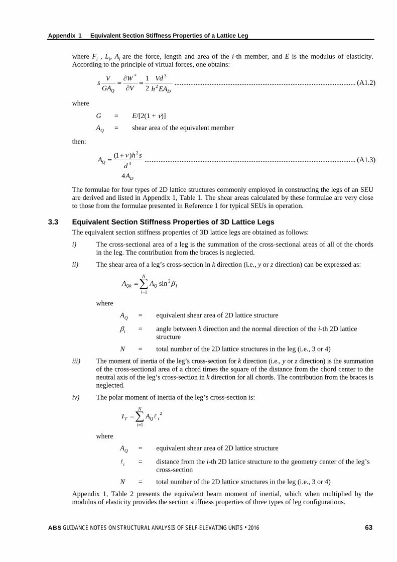
Appendix 1 Equivalent Section Stiffness Properties of a Lattice Leg
where Fi , Li, Ai are the force, length and area of the i-th member, and E is the modulus of elasticity. According to the principle of virtual forces, one obtains:
DQ EAhVd
VW
GAVs 2
3*
21
=∂
∂= ....................................................................................................... (A1.2)
where
G = E/[2(1 + ν)]
AQ = shear area of the equivalent member
then:
D
Q
Ad
shA
4
)1(3
2ν+= ........................................................................................................................ (A1.3)
The formulae for four types of 2D lattice structures commonly employed in constructing the legs of an SEU are derived and listed in Appendix 1, Table 1. The shear areas calculated by these formulae are very close to those from the formulae presented in Reference 1 for typical SEUs in operation.
3.3 Equivalent Section Stiffness Properties of 3D Lattice Legs The equivalent section stiffness properties of 3D lattice legs are obtained as follows:
i) The cross-sectional area of a leg is the summation of the cross-sectional areas of all of the chords in the leg. The contribution from the braces is neglected.
ii) The shear area of a leg’s cross-section in k direction (i.e., y or z direction) can be expressed as:
i
N
iQQk AA β∑
=
=1
2sin
where
AQ = equivalent shear area of 2D lattice structure
βi = angle between k direction and the normal direction of the i-th 2D lattice structure
N = total number of the 2D lattice structures in the leg (i.e., 3 or 4)
iii) The moment of inertia of the leg’s cross-section for k direction (i.e., y or z direction) is the summation of the cross-sectional area of a chord times the square of the distance from the chord center to the neutral axis of the leg’s cross-section in k direction for all chords. The contribution from the braces is neglected.
iv) The polar moment of inertia of the leg’s cross-section is:
∑=
=N
iiQT AI
1
2
where
AQ = equivalent shear area of 2D lattice structure
i = distance from the i-th 2D lattice structure to the geometry center of the leg’s cross-section
N = total number of the 2D lattice structures in the leg (i.e., 3 or 4)
Appendix 1, Table 2 presents the equivalent beam moment of inertial, which when multiplied by the modulus of elasticity provides the section stiffness properties of three types of leg configurations.
ABS GUIDANCE NOTES ON STRUCTURAL ANALYSIS OF SELF-ELEVATING UNITS . 2016 63
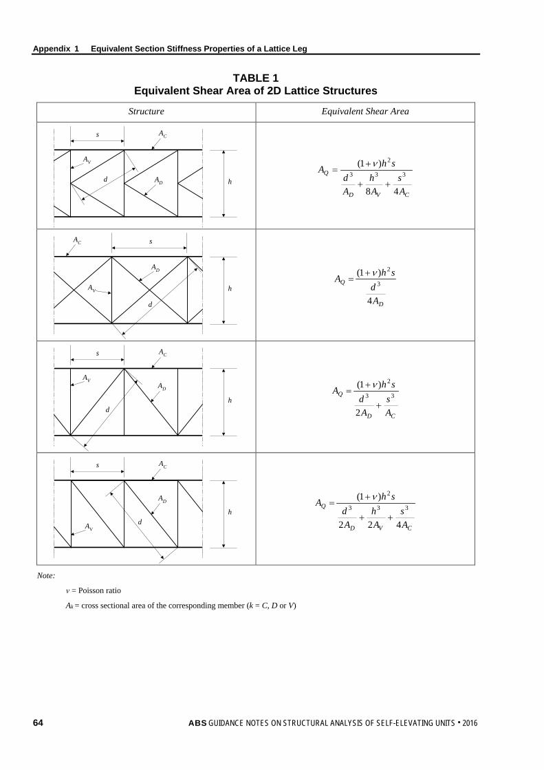
Appendix 1 Equivalent Section Stiffness Properties of a Lattice Leg
TABLE 1 Equivalent Shear Area of 2D Lattice Structures
Structure Equivalent Shear Area
AC
AD
AV
s
d h
CVD
Q
As
Ah
Ad
shA
48
)1(333
2
++
+=
ν
s
h
AC
AD
AV
d
D
Q
Ad
shA
4
)1(3
2ν+=
ACs
h
AD
AV
d
CD
Q
As
Ad
shA 33
2
2
)1(
+
+=
ν
ACs
hd
AD
AV
CVD
Q
As
Ah
Ad
shA
422
)1(333
2
++
+=
ν
Note:
ν = Poisson ratio
Ak = cross sectional area of the corresponding member (k = C, D or V)
64 ABS GUIDANCE NOTES ON STRUCTURAL ANALYSIS OF SELF-ELEVATING UNITS . 2016
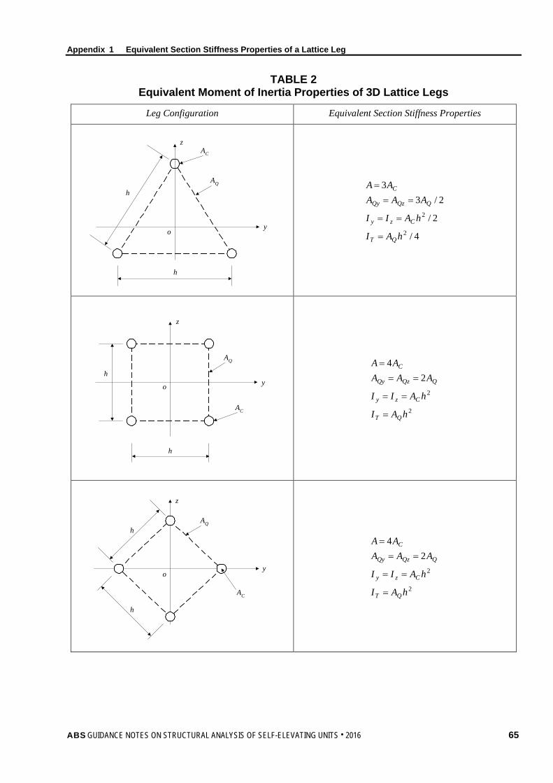
Appendix 1 Equivalent Section Stiffness Properties of a Lattice Leg
TABLE 2 Equivalent Moment of Inertia Properties of 3D Lattice Legs
Leg Configuration Equivalent Section Stiffness Properties
AC
AQ
h
h
oy
z
4/
2/
2/33
2
2
hAI
hAII
AAAAA
QT
Czy
QQzQy
C
=
==
===
h
h
AC
AQ
o
z
y
2
2
24
hAI
hAII
AAAAA
QT
Czy
QQzQy
C
=
==
===
h
h
o
AC
AQ
z
y
2
2
24
hAI
hAII
AAAAA
QT
Czy
QQzQy
C
=
==
===
ABS GUIDANCE NOTES ON STRUCTURAL ANALYSIS OF SELF-ELEVATING UNITS . 2016 65
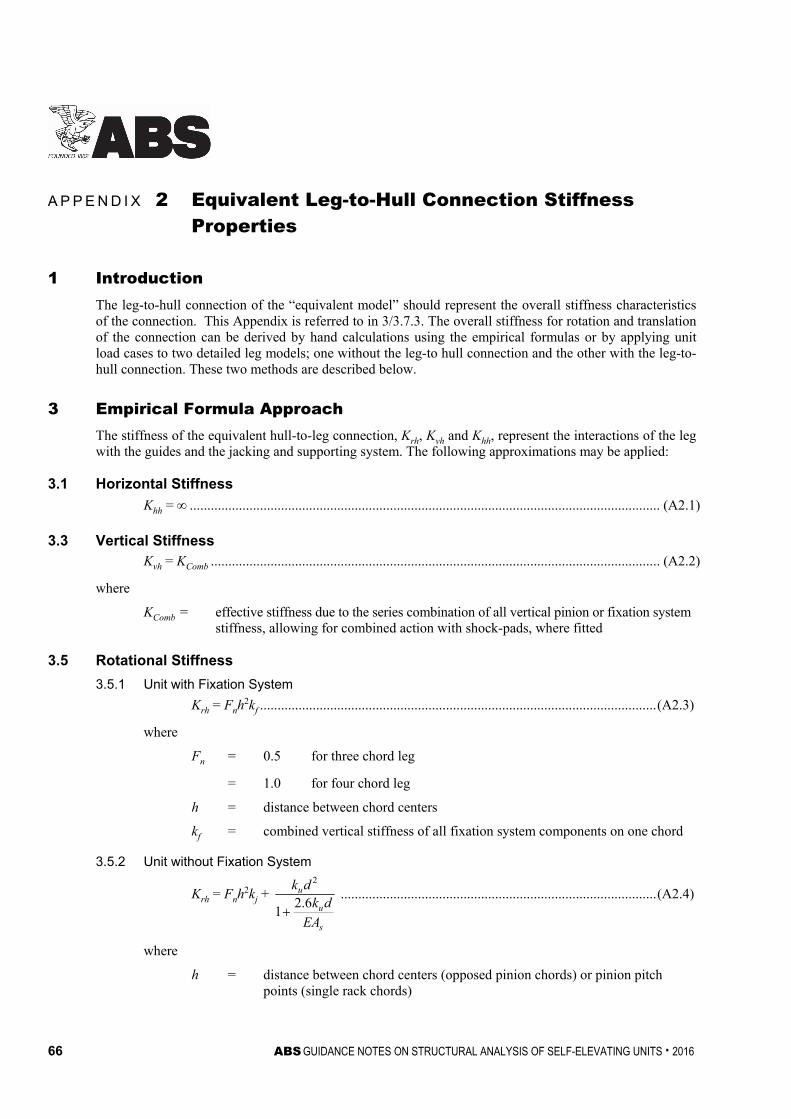
66 ABS GUIDANCE NOTES ON STRUCTURAL ANALYSIS OF SELF-ELEVATING UNITS . 2016
A p p e n d i x 2 : E q u i v a l e n t L e g - t o - H u l l C o n n e c t i o n S t i f f n e s s P r o p e r t i e s
A P P E N D I X 2 Equivalent Leg-to-Hull Connection Stiffness Properties
1 Introduction The leg-to-hull connection of the “equivalent model” should represent the overall stiffness characteristics of the connection. This Appendix is referred to in 3/3.7.3. The overall stiffness for rotation and translation of the connection can be derived by hand calculations using the empirical formulas or by applying unit load cases to two detailed leg models; one without the leg-to hull connection and the other with the leg-to-hull connection. These two methods are described below.
3 Empirical Formula Approach The stiffness of the equivalent hull-to-leg connection, Krh, Kvh and Khh, represent the interactions of the leg with the guides and the jacking and supporting system. The following approximations may be applied:
3.1 Horizontal Stiffness
Khh = ...................................................................................................................................... (A2.1)
3.3 Vertical Stiffness Kvh = KComb ................................................................................................................................ (A2.2)
where
KComb = effective stiffness due to the series combination of all vertical pinion or fixation system stiffness, allowing for combined action with shock-pads, where fitted
3.5 Rotational Stiffness
3.5.1 Unit with Fixation System
Krh = Fnh2kf ................................................................................................................. (A2.3)
where
Fn = 0.5 for three chord leg
= 1.0 for four chord leg
h = distance between chord centers
kf = combined vertical stiffness of all fixation system components on one chord
3.5.2 Unit without Fixation System
Krh = Fnh2kj +
s
u
u
EA
dkdk6.2
1
2
.......................................................................................... (A2.4)
where
h = distance between chord centers (opposed pinion chords) or pinion pitch points (single rack chords)
Appendix 2 Equivalent Leg-to-Hull Connection Stiffness Properties
5 Unit Load Approach
The unit load method described in Appendix 1 can also be used for deriving the stiffness properties of the equivalent leg-to-hull connection by applying unit loads, as described below, to a detailed leg model without the leg-to-hull connection and the other detailed leg model combined with the leg-to-hull connection. The differences in deflections and rotations between these two models can be used to determine the stiffness properties of the equivalent leg-to-hull connection. The following unit load cases should be used:
5.1 Unit Axial Load Case This case determines the vertical leg-to-hull connection stiffness, Kvh, based on the difference in axial deflections between the detailed leg model, ∆, and the combined leg and leg-to-hull connection model, ∆C, under the unit axial load, F:
Kvh = F/(∆C – ∆) ......................................................................................................................... (A2.5)
5.3 Unit Moment Case This case determines the rotational connection stiffness, Krh, based on the difference in the end slopes between the detailed model, θ, and the combined leg and leg-to-hull connection model, θC, under the unit moment, M:
Krh = M/(θC – θ) ......................................................................................................................... (A2.6)
Alternatively, the rotational stiffness can also be derived based on the difference in the end deflections between the detailed model, δ, and the combined leg and leg-to-hull connection model, δC, under unit moment, M:
Krh = ML/(δC – δ) ....................................................................................................................... (A2.7)
5.5 Unit Shear Load Case This case determines the horizontal leg-hull connection stiffness, Khh, in a similar manner, accounting for the rotational stiffness already derived. Normally the horizontal leg-to-hull connection stiffness may be assumed infinite.
ABS GUIDANCE NOTES ON STRUCTURAL ANALYSIS OF SELF-ELEVATING UNITS . 2016 67
A p p e n d i x 3 : R e f e r e n c e s
A P P E N D I X 3 References
1. Guidelines for Site Specific Assessment of Mobile Jack-Up Units, Technical & Research Bulletin 5-5A, SNAME, Published in January 2002
2. Rules for Building and Classing Mobile Offshore Drilling Units, Part 3, ABS, 2013
3. Dynamics of Structures, Second Edition, R. Clough and J. Penzien, 1993
4. Stochastic Response of Fixed Offshore Structures in Random Sea, Research Report R78-37, Department of Civil Engineering, MIT, 1978
5. Teughels, Anne, Continuum Models for Beam and Platelike Lattice Structures, IASS-IACM 2000, Fourth International Colloquium on Computation of Shell and Spatial Structures, Chania – Crete, Greece, June 5-7, 2000
6. ISO Standard 19905-1 Petroleum and natural gas industries – Site-specific assessment of mobile offshore units – Part 1: Jack-ups
7. Perry, M.J. and Mobbs, B, Factoring to Improve Conservatism of the Drag-inertia Method When Determining Dynamic Amplification of Jackup Units, Proc. 30th Int. Conf. on Ocean, Offshore and Arctic Engineering (OMAE), Rotterdam, The Netherland, OMAE2011-50335, 19-24 June 2011
8. Lu, Y., Chen, Y.N., Tan, P.L., Bai, Y., Prediction of Jack-Up Response, Proc. 20th Int. Conf. on Offshore Mechanic and Arctic Engineering (OMAE), Rio de Janeiro, Brazil, 2001
9. Guidance Notes on Dynamic Analysis Procedure for Self-Elevating Units, ABS, 2014
10. Guide for the Fatigue Assessment of Offshore Structures, ABS, 2003
11. Guide for the Buckling and Ultimate Strength Assessment for Offshore Structures, ABS, 2004
68 ABS GUIDANCE NOTES ON STRUCTURAL ANALYSIS OF SELF-ELEVATING UNITS . 2016