STRICTLY CONFIDENTIAL

2015 EXAMINATIONS

ACCOUNTING TECHNICIAN PROGRAMME

PAPER TC3: BUSINESS MATHEMATICS & STATISTICS

WEDNESDAY 3 JUNE 2015 TIME ALLOWED : 3 HOURS

SUGGESTED SOLUTIONS

1

1. (a)

3

385

4132

22

=

333

332

22

,

= 33

32

,

= 033 ,

(b) Given that 20A , 6B , 4C and 5D ,

then

DCB

CBAM

243

1042

=

524463

41046202

,

= 101618

6240

,

= 4012

480

2. (a) Frequency distribution,

No. of unprocessed

invoices (x)

Tally marks Frequency (f)

0 1

2 3

4 5 6

||| ||||

|||| |||| |||

||| || |

3 5

4 8

3 2 1

Total 26

(b) Mean number and standard deviation of invoices left unprocessed:

x f xf 2xf

0 3 0 0

1 5 5 5

2 4 8 16

3 8 24 72

4 3 12 48

5 2 10 50

6 1 6 36

26 65 227

2

Hence,

(i) Mean number of invoices left unprocessed is

f

xf5.2

26

65 invoices

(ii) Standard deviation of invoices left unprocessed is

22

f

xf

f

xf=

2

26

65

26

227

,

= 1.58 invoices

3. (a) 100305 2 xxxC

(i) The cost ofproducing 8 shirts is:

100830858 2 C = 320 – 240 +100 = 180

= K18,000

(ii) Minimum cost: Completing the square,

2065100305 22 xxxxxC ,

= 2033 22x ,

Minimum occurs when 03 x i.e. when 3x i.e. 3 shirts. Alternatively,

3010 xxC

Minimum occurs when 0 xC

i.e. 03010 x

3010 x

3x i.e. 3 shirts.

(b) (i) P(person will not select a category D vehicle pamphlet) = 1 – P(person selects Category D vehicle pamphlet),

= 94.0500

470

500

301 ,

(ii) P(Category B vehicle or a Category C vehicle pamphlet is selected) = P(B or C)

= CBPCPBP ,

= CPBP since B and C are mutually exclusive

= 500

150

500

265 = 83.0

500

415 .

3

4. (a) (i) Depreciation is the loss of value of an item of an asset over a period of time as it is being used. For example, the value of a car will go down as it

is being used.

Or Alternatively, depreciation is an allowance made in

estimates, valuations or balance sheets, normally for wear and tear.

(ii) Here present value is P = K500,000, 06.0r and future value is K150,000.

Need n such that 15000006.01500000 n

i.e. 500000

15000094.0

n

or 10

394.0

n

Taking logs: 10

3log94.0log

n

10

3log94.0log n ,

or 46.1994.0log

3.0logn

i.e. it will take approximately 19.5 years

(b) 60412 yx

4084 yx

The augmented matrix is

40

60

84

412and 80169644812

84

412 ,

Then

84

412

840

460

x = 480

320

80

160480

80

440860

,

84

412

404

6012

y = 380

240

80

240480

80

6044012

,

4

5. (a) Continuous data are data that can take any value within a range while discrete data are data that can only take certain fixed and finite values.

(b) (i) Calculation of percentages:

Item Amount Percentage

Food 55000 35

Utilities 15000 10

Transport 25000 16

School fees 40000 26

Entertainment 20000 13

Sum 155000 100

Simple percentage bar chart

M1 (Labelled axes), (Correct bars)

(ii) VAT on non-food items = %5.16 of (K155,000 – K55,000),

= 500,16000,100100

5.16KK ,

0

5

10

15

20

25

30

35

40

Food Utilities Transport School fees Entertainment

Pe

rce

nta

ge

Budget Item

5

6. (a) Let x be the number of tables the carpenter makes.

(i) Then his cost = 500,18500,2000,4750 x = 000,25750 x ,

Revenue (sales) = x950,1

Then profit is = x950,1 - 000,25750 x = 000,251200 x ,

(ii) To make a profit of K11,000, we need

11000250001200 x ,

25000110001200 x ,

360001200 x

301200

36000x

i.e. he needs to make 30 tables to make a profit of K11,000

(b) Profit index numbers using 2011 as base year

Year 2009 2010 2011 2012 2013

Profit

(K

million

9.641005.18

12 6.81100

5.18

1.15 100100

5.18

5.18 107100

5.18

8.19 6.87100

5.18

2.16

SECTION B (40 Marks)

7. (a) (i) Systematic sampling is a quasi-random sampling technique ideal for

populations that are clearly structured and involves taking the first item

randomly and subsequently picking every other k-th item. On the other hand, judgmental sampling is a non-random sampling in which the

researcher uses his/her knowledge, experience and judgment as to which items to include in the sample.

(ii) Advantages:

(1) Systematic sampling: easy to conduct for certain types of population.

(2) Judgmental sampling: experience can be used to ensure a good sample selection.

Disadvantages:

(1) Systematic sampling: it cannot apply to all types of population.

6

(2) Judgmental sampling: the method is not random and can lead to bias.

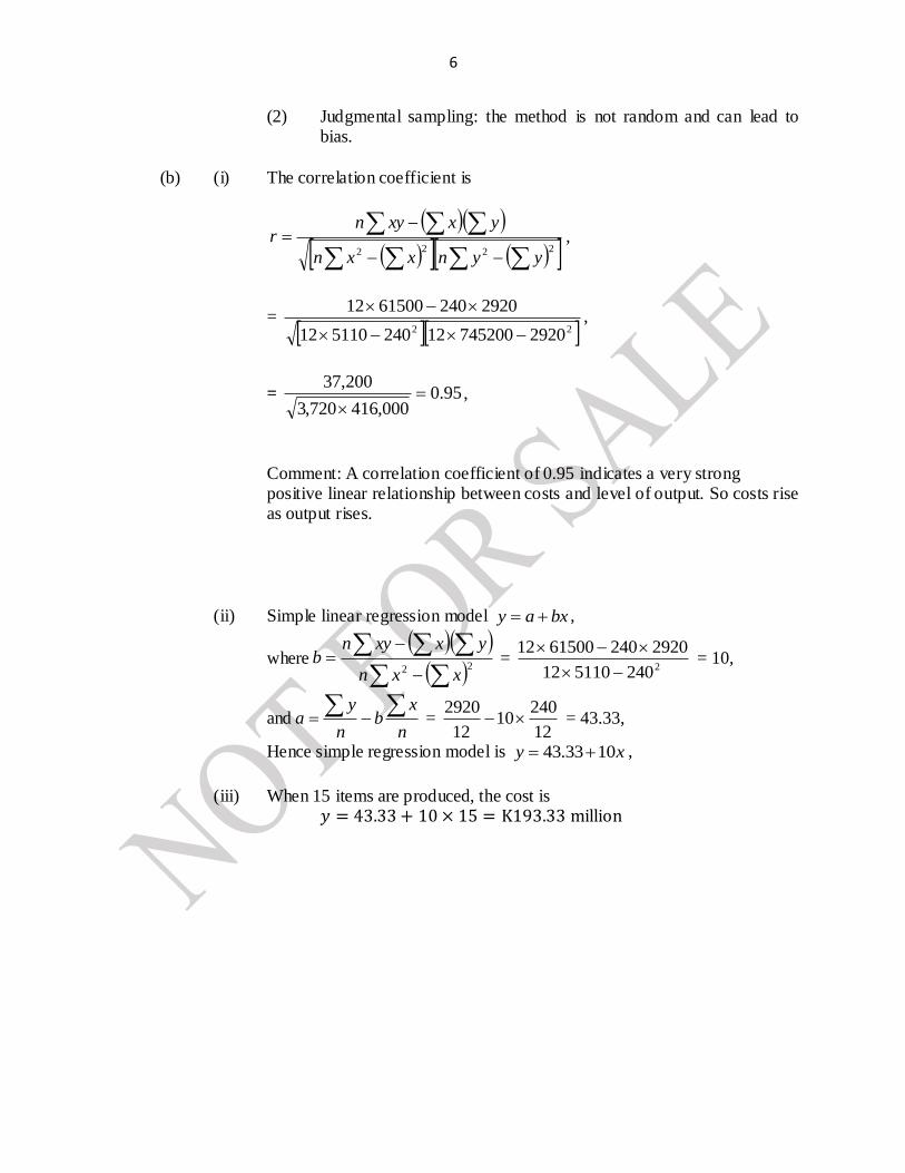
(b) (i) The correlation coefficient is

2222

yynxxn

yxxynr ,

= 22 292074520012240511012

29202406150012

,

= 95.0000,416720,3

200,37

,

Comment: A correlation coefficient of 0.95 indicates a very strong positive linear relationship between costs and level of output. So costs rise as output rises.

(ii) Simple linear regression model bxay ,

where 22

xxn

yxxynb =

2240511012

29202406150012

= 10,

andn

xb

n

ya

=

12

24010

12

2920 = 43.33,

Hence simple regression model is xy 1033.43 ,

(iii) When 15 items are produced, the cost is

7

8. (a) (i) Any two components that make up a time series:

I. Trend: the trend in a time series is the general, overall movement of the series or variable series, with any sharp fluctuations largely smoothed out.

II. Seasonal variation: the seasonal component accounts for the regular

variations that certain variables show at various times of the year or influenced by seasons.

(Others: cyclic variation, irregular or random variation)

(ii) I. Scatter diagram

0

10

20

30

40

50

60

70

Qtr

1 Qtr

2 Qtr

3 Qtr

4 Qtr

1 Qtr

2 Qtr

3 Qtr

4 Qtr

1 Qtr

2 Qtr

3 Qtr

4

Sale

s (K

'000

)

Year

2012 2013 2014

8

II. Moving averages trend values

Year Quarter Sales

Moving

total

Moving

average

Centred MA

(trend values)

2011

1 42

2 41

174 43.5

3 52

43.875

177 44.25

4 39

45.125

184 46

2012

1 45

47.125

193 48.25

2 48

49.125

200 50

3 61

50.875

207 51.75

4 46

52.125

210 52.5

2013

1 52

52.375

209 52.25

2 51

52.25

209 52.25

3 60

4 46

(b) From tables, the cumulative present value factor for a constant inflow at 15% for 5 years is 3.3522,

Or

PV

Hence the NPV of investment A is 044,673522.3000,20 KK .

Alternatively,

r

rPMTPV

n

11

= 10.043,6715.0

15.11000,20

5

K

,

As the other two investments do not involve constant inflows, and so the PVs for individual years have tobe summed as follows:

9

Year (end)

Discount

factor

Investment B Investment C

Inflow (K) PV Inflow PV

1 0.8696 10,000 8,696.00 40,000 34,784

2 0.7561 15,000 11,341.50 30,000 22,683

3 0.6575 20,000 13,150.00 20,000 13,150

4 0.5718 25,000 14,295.00

5 0.4972 30,000 14,916.00

NPV 62,398.50 70,617

The NPV for investments A, B and C are K67,044, K62,398.50 and K70,617

respectively. Then Investment C should be chosen since it yields the highest NPV.

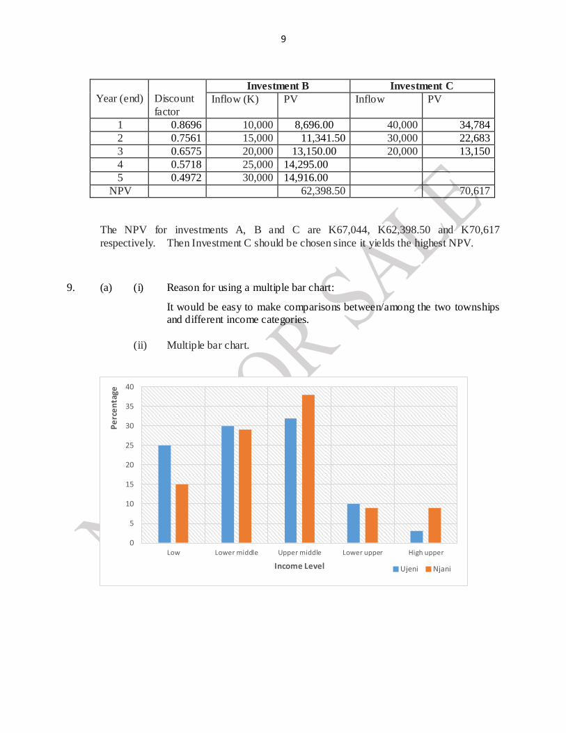
9. (a) (i) Reason for using a multiple bar chart:

It would be easy to make comparisons between/among the two townships and different income categories.

(ii) Multiple bar chart.

0

5

10

15

20

25

30

35

40

Low Lower middle Upper middle Lower upper High upper

Pe

rce

nta

ge

Income Level Ujeni Njani

10

(b) (i) Linear programming model for monthly production:

Let x = number of Ndixia models produced

Let y = number of Zude models produced

Summary of information provided:

Item/Activity Ndixia Zude Resource availability

Assembly Testing Tubes Zude

8 2 0

10 5 1

2000 hours 600 hours 100 tubes

Cost Selling Price

7,500 12,500

24,000 31,000

Profit 5,000 7,000

Hence LP model is:

Maximise yxP 70005000 ,

subject to

2000108 yx

60052 yx ,

100y ,

0, yx

(ii) Graphical solution: Sketching straight line graphs:

I: 2000108 yx i.e. 2000108 yx

when 0x , 200y

0y , 250x

II: I: 60052 yx i.e. 60023 yx

when 0x , 120y

0y , 300x

III: 100y , 100y

11

(Not drawn to scale)

(Sketching feasible region)

Checking all the vertices, the optimal solution is found at Q where 40y and 200x .

Hence Ung’onoung’ono Ltd should produce 200 Ndixia model TV sets and 40 Zude model TV sets to get a maximum profit of

000,280,14070002005000 KP .

E N D