Embed Size (px)
Citation preview

STRICHARTZ ESTIMATES AND THE NONLINEAR
SCHRODINGER EQUATION ON MANIFOLDS WITH
BOUNDARY
MATTHEW D. BLAIR, HART F. SMITH, AND CHRIS D. SOGGE
Abstract. We establish Strichartz estimates for the Schrodinger equation onRiemannian manifolds (Ω, g) with boundary, for both the compact case and
the case that Ω is the exterior of a smooth, non-trapping obstacle in Euclidean
space. The estimates for exterior domains are scale invariant; the range ofLebesgue exponents (p, q) for which we obtain these estimates is smaller than
the range known for Euclidean space, but includes the key L4tL
∞x estimate,
which we use to give a simple proof of well-posedness results for the energycritical Schrodinger equation in 3 dimensions. Our estimates on compact man-
ifolds involve a loss of derivatives with respect to the scale invariant index. We
use these to establish well-posedness for finite energy data of certain semilinearSchrodinger equations on general compact manifolds with boundary.
1. Introduction
Let (Ω, g) be a Riemannian manifold with boundary, of dimension n ≥ 2, and letv(t, x) : [0, T ]× Ω→ C be the solution to the Schrodinger equation
(i∂t + ∆g)v(t, x) = 0 , v(0, x) = f(x) . (1)
We assume in addition that v satisfies either Dirichlet or Neumann boundary con-ditions
v(t, x)∣∣∂Ω
= 0 or ∂νv(t, x)∣∣∂Ω
= 0 ,
where ∂ν denotes the normal derivative along the boundary. In this work, weconsider local in time Strichartz estimates for such solutions; these are a family ofspace-time integrability estimates of the form
‖v‖Lp([0,T ];Lq(Ω)) ≤ C‖f‖Hs(Ω) . (2)
Here Hs(Ω) denotes the L2 Sobolev space of order s, defined with respect to thespectral resolution of either the Dirichlet or Neumann Laplacian. The Lebesgueexponents will always be taken to satisfy p, q ≥ 2, and always the Sobolev indexsatisfies s ≥ 0.
The consideration of high frequency bump function solutions to (1) shows thatp, q, s must satisfy
2
p+n
q≥ n
2− s . (3)
The authors were supported by National Science Foundation grants DMS-0801211, DMS-0654415, and DMS-0555162.
1
2 MATTHEW D. BLAIR, HART F. SMITH, AND CHRIS D. SOGGE
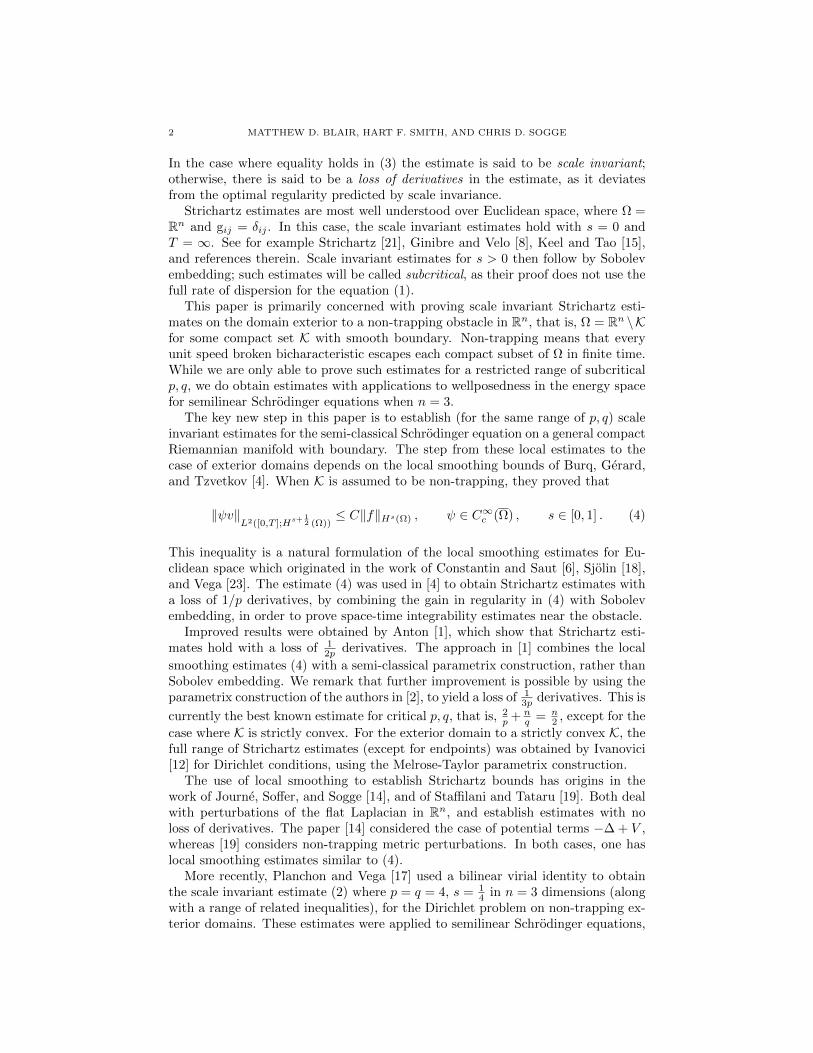
In the case where equality holds in (3) the estimate is said to be scale invariant;otherwise, there is said to be a loss of derivatives in the estimate, as it deviatesfrom the optimal regularity predicted by scale invariance.
Strichartz estimates are most well understood over Euclidean space, where Ω =Rn and gij = δij . In this case, the scale invariant estimates hold with s = 0 andT = ∞. See for example Strichartz [21], Ginibre and Velo [8], Keel and Tao [15],and references therein. Scale invariant estimates for s > 0 then follow by Sobolevembedding; such estimates will be called subcritical, as their proof does not use thefull rate of dispersion for the equation (1).
This paper is primarily concerned with proving scale invariant Strichartz esti-mates on the domain exterior to a non-trapping obstacle in Rn, that is, Ω = Rn \Kfor some compact set K with smooth boundary. Non-trapping means that everyunit speed broken bicharacteristic escapes each compact subset of Ω in finite time.While we are only able to prove such estimates for a restricted range of subcriticalp, q, we do obtain estimates with applications to wellposedness in the energy spacefor semilinear Schrodinger equations when n = 3.
The key new step in this paper is to establish (for the same range of p, q) scaleinvariant estimates for the semi-classical Schrodinger equation on a general compactRiemannian manifold with boundary. The step from these local estimates to thecase of exterior domains depends on the local smoothing bounds of Burq, Gerard,and Tzvetkov [4]. When K is assumed to be non-trapping, they proved that
‖ψv‖L2([0,T ];Hs+
12 (Ω))
≤ C‖f‖Hs(Ω) , ψ ∈ C∞c (Ω) , s ∈ [0, 1] . (4)
This inequality is a natural formulation of the local smoothing estimates for Eu-clidean space which originated in the work of Constantin and Saut [6], Sjolin [18],and Vega [23]. The estimate (4) was used in [4] to obtain Strichartz estimates witha loss of 1/p derivatives, by combining the gain in regularity in (4) with Sobolevembedding, in order to prove space-time integrability estimates near the obstacle.
Improved results were obtained by Anton [1], which show that Strichartz esti-mates hold with a loss of 1
2p derivatives. The approach in [1] combines the local
smoothing estimates (4) with a semi-classical parametrix construction, rather thanSobolev embedding. We remark that further improvement is possible by using theparametrix construction of the authors in [2], to yield a loss of 1
3p derivatives. This is
currently the best known estimate for critical p, q, that is, 2p + n
q = n2 , except for the
case where K is strictly convex. For the exterior domain to a strictly convex K, thefull range of Strichartz estimates (except for endpoints) was obtained by Ivanovici[12] for Dirichlet conditions, using the Melrose-Taylor parametrix construction.
The use of local smoothing to establish Strichartz bounds has origins in thework of Journe, Soffer, and Sogge [14], and of Staffilani and Tataru [19]. Both dealwith perturbations of the flat Laplacian in Rn, and establish estimates with noloss of derivatives. The paper [14] considered the case of potential terms −∆ + V ,whereas [19] considers non-trapping metric perturbations. In both cases, one haslocal smoothing estimates similar to (4).
More recently, Planchon and Vega [17] used a bilinear virial identity to obtainthe scale invariant estimate (2) where p = q = 4, s = 1
4 in n = 3 dimensions (alongwith a range of related inequalities), for the Dirichlet problem on non-trapping ex-terior domains. These estimates were applied to semilinear Schrodinger equations,

STRICHARTZ ESTIMATES ON MANIFOLDS WITH BOUNDARY 3
showing that for defocusing, energy subcritical nonlinearities, one has global ex-istence for initial data in H1(Ω). For strictly convex K, the work [12] establishesglobal existence for the energy critical semilinear equation, focusing or defocusing,for small Dirichlet data in H1(Ω).
In the present work, we establish the Strichartz estimates (2) for a range ofsubcritical p, q. The key tool is a microlocal parametrix construction previouslyused for the wave equation in [20] and [3]. This approach treats both Dirichlet andNeumann boundary conditions, and applies to general non-trapping obstacles.
Theorem 1.1. Let Ω = Rn \ K be the exterior domain to a compact non-trappingobstacle with smooth boundary, and ∆ the standard Laplace operator on Ω, subjectto either Dirichlet or Neumann conditions. Suppose that p > 2 and q <∞ satisfy
3p + 2
q ≤ 1 , n = 2 ,1p + 1
q ≤12 , n ≥ 3 .
(5)
Then for the solution v = exp(it∆)f to the Schrodinger equation (1), the followingestimates hold
‖v‖Lp([0,T ];Lq(Ω)) ≤ C‖f‖Hs(Ω) , (6)
provided that2
p+n
q=n
2− s . (7)
For Dirichlet boundary conditions, the estimates hold with T =∞.
That one may take T = ∞ in (6) for Dirichlet boundary conditions is a conse-quence of the fact that (4) holds for T =∞ in the Dirichlet case.
We now consider estimates for compact Riemannian manifolds Ω, with ∆g theLaplace-Beltrami operator for g. Burq, Gerard, and Tzvetkov showed in [5] thatfor p > 2 estimates hold with a loss of 1
p derivatives in case ∂Ω = ∅. The same
result was established for compact manifolds with geodesically concave boundaryin [12]. For general boundaries, we establish estimates with the same loss of 1
p
derivatives, valid for (p, q) satisfying (5). For such (p, q), this is an improvementover the estimates of [2], which involve a loss of 4
3p derivatives.
Theorem 1.2. Let Ω be a compact Riemannian manifold with boundary. Supposethat p > 2 and q < ∞ satisfy (5). Then for the solution v = exp(it∆g)f to theSchrodinger equation (1), the following estimates hold for fixed finite T
‖v‖Lp([0,T ];Lq(Ω)) ≤ C‖f‖Hs+ 1
p (Ω)
for p, q, s satisfying (7).
As with [5] and [12, Corollary 1.5], the loss of 1p arises as a consequence of using
a representation for solutions that is valid only in a local coordinate chart; that is,on a semi-classical time scale.
In the last two sections of this paper we present applications of the above the-orems to well-posedness of semilinear Schrodinger equations in three space dimen-sions with finite energy data. In Section 5, we use Theorem 1.1 and interpolationto establish the L4
tL∞x Strichartz estimate. This estimate yields a simple proof
of well-posedness for small energy data to the energy critical equation on exteriordomains, a result first established by Ivanovici and Planchon [13]. In Section 6, weestablish a variant in three dimensions of Theorem 1.2 for the case p = 2, for data

4 MATTHEW D. BLAIR, HART F. SMITH, AND CHRIS D. SOGGE
u localized to dyadic frequency scale λ. The estimate involves a loss of (log λ)2
relative to the estimates of [5]. Following the Yudovitch argument as in [5, Sec-tion 3.3], we use this to establish well-posedness for finite energy data to certainsemilinear Schrodinger equations, on general three dimensional compact manifoldswith boundary. The logarithmic loss in the estimates restricts our result to slowergrowth nonlinearities than considered in [5] for manifolds without boundary. Forparticular three dimensional manifolds without boundary, recent results have beenobtained for the energy critical case by Herr [9], Herr, Tataru, and Tzvetkov [10],and Ionescu and Pausader [11].
The outline of this paper is as follows. In section 2, we reduce Theorems 1.1-1.2to estimates on the unit scale within a single coordinate chart. Section 3 outlines theangular localization approach from [20], and introduces a wave packet parametrixconstruction. Estimates on the parametrix are then developed in section 4. Weconclude in sections 5 and 6 with the applications to semilinear Schrodinger equa-tions.
Throughout this paper we use the following notation. The expression X . Ymeans that X ≤ CY for some C depending only on the manifold, metric, andpossibly the triple (p, q, s) under consideration. Also, we abbreviate Lp(I;Lq(U))by LpLq(I × U) or by LpTL
q(U) when I = [0, T ]. If U = Rn we write LpTLq. As
will be seen below, the last component of an n-vector will take on special meaning,hence we will often write x = (x′, xn) so that x′ denotes the first n−1 components.
We conclude this introduction with a remark on the Sobolev spaces that we usein the case of exterior domains. In the above theorems, the Sobolev space Hs(Ω)and the operator exp(it∆) are defined using the spectral resolution of ∆ subject tothe chosen Dirichlet or Neumann boundary condition B; in particular, the linearevolution preserves Hs(Ω). The space H2(Ω) is then equal to the subspace ofH2(Ω) satisfying Bu = 0, and for 0 ≤ s ≤ 2, the space Hs(Ω) can be defined byinterpolation. For s ≥ 2, these spaces satisfy u ∈ Hs(Ω) if and only if Bu = 0and ∆u ∈ Hs−2(Ω). Thus, for large values of s, a function in Hs(Ω) satisfies thelinear compatibility conditions B(∆ku) = 0, for k for which this is defined. Thesecompatibility conditions are necessary to bootstrap the local smoothing estimates(4) to higher orders s, as well as to insure v(t, · ) ∈ Hs(Ω), which is required tohandle commutator terms with cutoff functions. We will also use that
‖v‖Hs(Ω) ≈ ‖ψv‖Hs(Ω) + ‖(1− ψ)v‖Hs(Rn) ,
where ψ ∈ C∞c (Ω) is such that 1 − ψ vanishes on a neighborhood of ∂Ω, and Ω isa compact manifold with boundary in which Ω∩ supp(ψ) embeds isometrically; for
example Ω = Ω ∩ [−R,R ]n with periodic boundary conditions and R sufficientlylarge.
We use Hs(Ω) to denote the space of extendable elements, with no boundaryconditions. For Ω an exterior domain, Hs(Ω) consists of restrictions of functionsin Hs(Rn) to Ω with the quotient norm (minimal norm of an extension); for Ωcompact we embed Ω in a compact manifold Ω′ without boundary, and Hs(Ω)consists of restrictions of elements Hs(Ω′). By elliptic regularity, Hs(Ω) ⊂ Hs(Ω).

STRICHARTZ ESTIMATES ON MANIFOLDS WITH BOUNDARY 5
2. Preliminary reductions
In this section, we reduce the inequalities in Theorems 1.1 and 1.2 to estimates onsolutions to a pseudodifferential equation defined in a coordinate chart near theboundary. We start by considering the case of Theorem 1.1.
For Ω = Rn \K, we take ψ ∈ C∞c (Ω) such that 1−ψ vanishes on a neighborhoodof ∂Ω = ∂K. Then v0 = (1−ψ)v satisfies the inhomogeneous Schrodinger equationon Rn: (
i∂t + ∆)v0 = [ψ,∆]v , v0|t=0 = (1− ψ)f .
Here, (1− ψ)f ∈ Hs(Rn), and by (4) we have [∆, ψ]v ∈ L2TH
s− 12 (Rn). (Although
stated only for s ∈ [0, 1] in [4], it is easy to see by a bootstrap argument andinterpolation that (4) holds for all s ≥ 0, where Hs is the is the intrinsic Sobolevspace for the Dirichlet/Neumann conditions as above.) The Strichartz estimatesfor v0 then follow from Proposition 2.10 of [4] together with Sobolev embedding.While [4] considers the case s ∈ [0, 1], the result of Proposition 2.10 of [4] followsfor all s > 0, since the free Schrodinger propagator exp(it∆) on Rn commutes withdifferentiation.
We are thus reduced to establishing estimates on the term ψv. We isometricallyembed a neighborhood of supp(ψ) into a compact manifold (Ω, g) with boundary,
where ∂Ω = ∂Ω. Then v1 = ψv satisfies the inhomogeneous Schrodinger equationon Ω: (
i∂t + ∆g
)v1 = [∆, ψ]v , v1|t=0 = ψf .
By (4), we are reduced to establishing the following estimate over a compact man-
ifold with boundary Ω,
‖v‖LpTLq(Ω) . ‖v‖L2TH
s+12 (Ω)
+ ‖(i∂t + ∆g)v‖L2TH
s− 12 (Ω)
. (8)
Here we use that [∆, ψ] vanishes near ∂Ω, hence maps Hs+ 12 (Ω)→ Hs− 1
2 (Ω).We next take a Littlewood-Paley decomposition of v in the x variable with
respect to the spectrum for ∆g. Precisely, we write
v = β0(−∆g) +
∞∑j=1
β(2−2j(−∆g)
)v ≡
∞∑j=0
vj ,
where∑∞j=1 β(2−2js) = 1 for s ≥ 2, and β is supported by s ∈ [ 1
2 , 2]. The lowfrequency terms are easily dealt with by Sobolev embedding, since the right handside of (8) controls the LpTH
s− 12 norm of v for 2 ≤ p ≤ ∞. The following square
function estimate holds, for example by heat kernel methods,
‖v‖LpTLq(Ω) ≈∥∥(∑
j |vj |2) 1
2∥∥LpTL
q(Ω)≤(∑
j ‖vj‖2LpTLq(Ω)
) 12
, (9)
where we use p, q ≥ 2 in the last step. By orthogonality, the desired estimate (8)would then follow as a consequence of the following estimate,
‖vj‖LpTLq(Ω) . 2j(s+12 )‖vj‖L2
TL2(Ω) + 2j(s−
12 )‖(i∂t + ∆g)vj‖L2
TL2(Ω) .
Finally, we divide [0, T ] into intervals of length 2−j and note that, since p, q ≥ 2,by the Minkowski inequality it suffices to prove the above on each subinterval; thatis, for T = 2−j . To summarize, Theorem 1.1 is thus reduced to establishing thefollowing semiclassical result.

6 MATTHEW D. BLAIR, HART F. SMITH, AND CHRIS D. SOGGE
Theorem 2.1. Let Ω be a compact Riemannian manifold with boundary, and ∆g
the Laplace-Beltrami operator, subject to either Dirichlet or Neumann boundaryconditions. Suppose that p > 2 and q <∞ satisfy (5) and (7).
Suppose also that, for all t, vλ(t, · ) is spectrally localized for −∆g to the range[ 14λ
2, 4λ2]. Then the following estimate holds, uniformly over λ,
‖vλ‖Lpλ−1L
q(Ω) . λs(λ
12 ‖vλ‖L2
λ−1L2(Ω) + λ−
12 ‖(i∂t + ∆g)vλ‖L2
λ−1L2(Ω)
). (10)
We observe that Theorem 1.2 also follows as a consequence of (10). To see this,we divide [0, T ] into subintervals of length λ−1, and note that for vλ = exp(it∆g)fλ,on each subinterval the right hand side of (10) is bounded by λs‖fλ‖L2(Ω). Summingthe Lp norm over a total of ≈ λ subintervals leads to
‖vλ‖LpTLq(Ω) . λs+ 1
p ‖fλ‖L2(Ω) ≈ ‖fλ‖Hs+ 1
p (Ω).
Applying the square function estimate (9) as above yields Theorem 1.2.We will establish (10) by the methods developed in [20] and [3] to obtain dis-
persive estimates for the wave equation on manifolds with boundary. We startby taking a finite partition of unity over Ω, subordinate to a cover by coordinatepatches. We restrict attention to a coordinate patch centered on ∂Ω; the interiorterms can be handled by the methods of [5], or by the parametrix construction ofthis paper. Thus, let ψ ∈ C∞c (Ω) be supported in a boundary normal coordinatepatch along ∂Ω. The function ψvλ is not sharply spectrally localized, but doesremain spectrally concentrated in frequencies ≤ λ. Precisely, for all k ≥ 0,
‖ψvλ‖L2λ−1H
k(Ω) . ‖vλ‖L2λ−1H
k(Ω) . λk‖vλ‖L2
λ−1L2(Ω) , (11)
and the same holds with vλ replaced by (i∂t + ∆g)vλ.Letting xn denote geodesic distance to the boundary, and x′ coordinates on ∂Ω,
in boundary normal coordinates the Laplace operator takes the form
∆gv = ρ−1∑
1≤i,j≤n
∂i(
gijρ ∂jv)
where ρ =√
det glk and gij denotes the inverse of the metric glk. Furthermore,gin = gni = δin, so there are no mixed ∂x′∂xn terms.
We now extend the metric g(x′, xn) in an even manner across xn = 0; thenew metric g(x′, |xn|), which we also denote by g, is defined on an open subset ofRn, and is of Lipschitz regularity. We extend the solution ψvλ in an odd or evenfashion, corresponding to Dirichlet or Neumann boundary conditions, to obtain aC1,1 function. We will assume ψ is chosen so that ψ(x′, xn) is independent of xnnear xn = 0. Since the extended Laplace operator is even, the regularity of g andvλ show that the extended solution satisfies the extended equation across xn = 0,
(i∂t + ∆g)(ψvλ) = [∆g, ψ]vλ + ψ(i∂t + ∆g)vλ ,
where ∆gvλ is extended oddly/evenly as is vλ, and ψ is even.By choosing sufficiently small coordinate patches, and rescaling if necessary, we
may assume that g extends to all of Rn, such that
‖gij − δij‖C0,1(Rn) ≤ c0 1 , gij = δij if |x| > 1 .
The odd (respectively even) extension operator maps functions in Hr(Rn+) satis-fying f(x′, 0) = 0 (respectively ∂xnf(x′, 0) = 0 ) to functions in Hr(Rn), provided

STRICHARTZ ESTIMATES ON MANIFOLDS WITH BOUNDARY 7
r ∈ [0, 52 ). The extension also commutes with differentiation in the x′ variables.
We observe that multiplication by functions such as g or ρ preserves Hr(Rn) forr ∈ [0, 3
2 ), and multiplication by ∂xρ preserves Hr(Rn) for r ∈ [0, 12 ). This can be
seen, e.g., from the fact that 〈ξ〉 12−ε is an A2 weight in one dimension, and that∂xρ is a Calderon-Zygmund type multiplier in xn.
It follows that the bound (11) holds to a limited extent for the extension of ψvλto Rn. To quantify this, we introduce the following family of norms, for r ≥ 0,
‖f‖Hr,λ =∑|α|≤N
(λ−|α|‖∂αx′f‖L2(Rn) + λ−|α|−r‖∂αx′f‖Hr(Rn)
),
and observe that ‖f‖Hσ,λ . ‖f‖Hr,λ if 0 ≤ σ ≤ r. Here N is taken to be a fixed butsufficiently large number, which we allow to change in a given inequality. However,for the results of this paper N need never exceed n+ 2.
By (11) and the above, it holds that for 2 ≤ r < 52
λ12 ‖ψvλ‖L2
λ−1Hr,λ(Rn) + λ−
12 ‖(i∂t + ∆g)(ψvλ)‖L2
λ−1Hr−2,λ(Rn)
. λ12 ‖vλ‖L2
λ−1L2(Ω) + λ−
12 ‖(i∂t + ∆g)vλ‖L2
λ−1L2(Ω) . (12)
This bound also holds if we replace ∆g on the left side by the divergence formoperator ∂ig
ij∂j , since the difference ρ−1(∂iρ)gij∂j maps Hr,λ → Hr−2,λ withnorm λ, provided r ∈ [2, 5
2 ). Since subsequent estimates will be only in terms of
the left hand side of (12), we may thus set ρ ≡ 1, and replace ∆g by∑ij ∂i gij∂j .
We next reduce matters to considering solutions that are strictly frequency lo-calized on Rn, and which satisfy an equation with frequency localized coefficients.For each µ, we form regularized coefficients gijµ by truncating the Fourier transform
of the gij so that
supp(gijµ ) ⊂ |ξ| ≤ cµ , (13)
for some small constant c. We observe the following estimates
‖gijµ − gij‖L∞(Rn) . µ−1, ‖∂αx gijµ ‖L∞(Rn) . µ
|α|−1 , |α| ≥ 1 . (14)
With slight abuse of notation we now set
∆gµv =∑
1≤i,j≤n
∂i(
gijµ ∂jv).
We will prove in the next section the following estimate for uµ(t, x) defined on[0, µ−1]× Rn, which are localized to spatial frequencies ≈ µ.
Lemma 2.2. Suppose that (p, q, s) are as in Theorem 1.1, and uµ(t, ξ) is supportedin the region 1
2µ ≤ |ξ| ≤52µ. Then
‖uµ‖Lpµ−1L
q . µs+12 ‖uµ‖L2
µ−1L2 + µs‖(i∂t + ∆gµ)uµ‖L1
µ−1L2 . (15)
Furthermore, if uµ(t, ξ) is in addition localized to |ξ′| ≤ 32 |ξn|, then (15) holds for
p > 2 and q <∞ satisfying (7) with s ≥ 0; that is, without the restriction (5).
In the remainder of this section we reduce (10), and hence Theorems 1.1 and1.2, to establishing Lemma 2.2.
We start by considering the frequency components µ ≤ λ of ψvλ (by which weunderstand its odd/even extension to Rn). Let βµ(D) denote a Littlewood-Paley

8 MATTHEW D. BLAIR, HART F. SMITH, AND CHRIS D. SOGGE
localization operator on Rn to frequencies ≈ µ, and consider uµ = βµ(D)(ψvλ).For µ ≤ λ, (15) and the Schwarz inequality imply
‖uµ‖Lpλ−1L
q . µs(λ
12 ‖uµ‖L2
λ−1L2 + λ−
12 ‖(i∂t + ∆gµ)uµ‖L2
λ−1L2
). (16)
Since s ≥ 0 in our bounds, we may sum over dyadic values of µ ≤ λ to establish(10) for the cutoff of ψvλ to frequencies ≤ λ, provided we bound the `2 norm overµ of the terms in parentheses in (16) by the terms in parentheses in (10). By (12),this is a special case of the following estimate, which we establish for all r ∈ [2, 5
2 ),(∑µ
λ‖uµ‖2L2λ−1H
r,λ + λ−1‖(i∂t + ∆gµ)uµ‖2L2λ−1H
r−2,λ
) 12
. λ12 ‖ψvλ‖L2
λ−1Hr,λ + λ−
12 ‖(i∂t + ∆g)(ψvλ)‖L2
λ−1Hr−2,λ . (17)
Since βµ is L2 bounded and commutes with differentiation, this will follow fromshowing the fixed time estimate(∑
µ
‖(βµ∆g −∆gµβµ)(ψvλ)‖2Hr−2,λ
) 12
. λ ‖ψvλ‖Hr−1,λ . (18)
In this estimate we may replace ∆g = ∂igij∂j by gij∂i∂j , and similarly for ∆gµ .
This follows since the difference (∂igij)∂j maps Hr−1,λ → Hr−2,λ with norm λ. By
the Coifman-Meyer commutator estimate (see [22, Prop 4.1D]), for σ ∈ [0, r − 2],(∑µ
‖ [βµ, g]∂2x(ψvλ)‖2Hσ
) 12
. ‖ψvλ‖Hσ+1 ≤ λσ+1 ‖ψvλ‖Hr−1,λ .
The same holds with [βµ,∆g] replaced by [∂x′ , [βµ,∆g]], since this has the effect ofdifferentiating the coefficients gij in x′, which remain Lipschitz. Hence(∑
µ
‖[βµ, g]∂2x(ψvλ)‖2Hr−2,λ
) 12
. λ ‖ψvλ‖Hr−1,λ .
Next, using (14) and interpolation, we obtain for 0 ≤ σ ≤ 1,(∑µ
‖(g − gµ)∂2xβµ(ψvλ)‖2Hσ
) 12
. ‖∂x(ψvλ)‖Hσ ≤ λσ+1 ‖ψvλ‖Hσ+1,λ .
Commuting with ∂x′ as above yields(∑µ
‖(g − gµ)∂2xβµ(ψvλ)‖2Hr−2,λ
) 12
. λ ‖ψvλ‖Hr−1,λ ,
completing the proof of (18).To handle frequencies µ > λ, we consider separately the tangential and normal
components of uµ. Thus, we decompose
βµ(ξ) = Γµ(ξ) + Γ′µ(ξ) ,
where
supp(Γµ) ⊂ ξ : |ξ′| ≤ 32 |ξn| , supp(Γ′µ) ⊂ ξ : |ξ′| ≥ |ξn| .
STRICHARTZ ESTIMATES ON MANIFOLDS WITH BOUNDARY 9
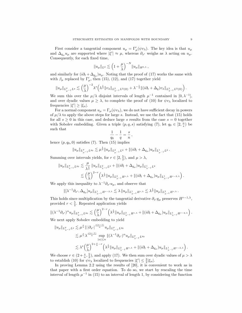
First consider a tangential component uµ = Γ′µ(ψvλ). The key idea is that uµand ∆gµuµ are supported where |ξ′| ≈ µ, whereas ∂x′ weighs as λ acting on uµ.Consequently, for each fixed time,
‖uµ‖L2 .(
1 +µ
λ
)−N‖uµ‖H0,λ ,
and similarly for (i∂t + ∆gµ)uµ. Noting that the proof of (17) works the same withwith βµ replaced by Γ′µ, then (15), (12), and (17) together yield
‖uµ‖Lpµ−1L
q .(µλ
)−2
λs(λ
12 ‖vλ‖L2
λ−1L2(Ω) + λ−
12 ‖(i∂t + ∆g)vλ‖L2
λ−1L2(Ω)
).
We sum this over the µ/λ disjoint intervals of length µ−1 contained in [0, λ−1],and over dyadic values µ ≥ λ, to complete the proof of (10) for ψvλ localized tofrequencies |ξ′| ≥ |ξn|.
For a normal component uµ = Γµ(ψvλ), we do not have sufficient decay in powersof µ/λ to apply the above steps for large s. Instead, we use the fact that (15) holdsfor all s ≥ 0 in this case, and deduce large s results from the case s = 0 togetherwith Sobolev embedding. Given a triple (p, q, s) satisfying (7), let q0 ∈ [2, ns ) besuch that
1
q0− 1
q=s
n,
hence (p, q0, 0) satisfies (7). Then (15) implies
‖uµ‖Lpµ−1L
q0 . µ12 ‖uµ‖L2
µ−1L2 + ‖(i∂t + ∆gµ)uµ‖L1
µ−1L2 .
Summing over intervals yields, for r ∈ [2, 52 ), and µ > λ,
‖uµ‖Lpλ−1L
q0 .µ
λ12
‖uµ‖L2λ−1L
2 + ‖(i∂t + ∆gµ)uµ‖L1λ−1L
2
.(µλ
)2−r(λ
12 ‖uµ‖L2
λ−1Hr,λ + ‖(i∂t + ∆gµ)uµ‖L1
λ−1Hr−2,λ
).
We apply this inequality to λ−1∂x′uµ, and observe that
‖[λ−1∂x′ ,∆gµ ]uµ‖L1λ−1H
r−2,λ . λ ‖uµ‖L1λ−1H
r,λ . λ12 ‖uµ‖L2
λ−1Hr,λ .
This holds since multiplication by the tangential derivative ∂x′gµ preserves Hr−1,λ,provided r < 5
2 . Repeated application yields
‖(λ−1∂x′)αuµ‖Lp
λ−1Lq0 .
(µλ
)2−r(λ
12 ‖uµ‖L2
λ−1Hr,λ + ‖(i∂t + ∆gµ)uµ‖L1
λ−1Hr−2,λ
).
We next apply Sobolev embedding to yield
‖uµ‖Lpλ−1L
q . µsn ‖ |∂x′ |
s(n−1)n uµ‖Lp
λ−1Lq0
. µsnλ
s(n−1)n sup
|α|≤n‖(λ−1∂x′)
αuµ‖Lpλ−1L
q0
. λs(µλ
)2+ sn−r(
λ12 ‖uµ‖L2
λ−1Hr,λ + ‖(i∂t + ∆gµ)uµ‖L1
λ−1Hr−2,λ
).
We choose r ∈ (2+ sn ,
52 ), and apply (17). We then sum over dyadic values of µ > λ
to establish (10) for ψvλ localized to frequencies |ξ′| ≤ 32 |ξn|.
In proving Lemma 2.2 using the results of [20], it is convenient to work as inthat paper with a first order equation. To do so, we start by rescaling the timeinterval of length µ−1 in (15) to an interval of length 1, by considering the function
10 MATTHEW D. BLAIR, HART F. SMITH, AND CHRIS D. SOGGE
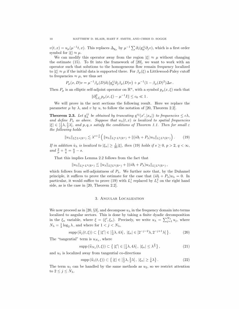
v(t, x) = uµ(µ−1t, x). This replaces ∆gµ by µ−1∑∂i(g
ijµ ∂jv), which is a first order
symbol for |ξ| ≈ µ.We can modify this operator away from the region |ξ| ≈ µ without changing
the estimate (15). To fit into the framework of [20], we want to work with anoperator such that solutions to the homogeneous flow remain frequency localizedto |ξ| ≈ µ if the initial data is supported there. For βµ(ξ) a Littlewood-Paley cutoffto frequencies ≈ µ, we thus set
Pµ(x,D)v = µ−1βµ(D)∂i(gijµ ∂jβµ(D)v
)+ µ−1(1− βµ(D)2)∆v .
Then Pµ is an elliptic self-adjoint operator on Rn, with a symbol pµ(x, ξ) such that
‖∂2ξiξjpµ(x, ξ)− µ−1I‖ ≤ c0 1 .
We will prove in the next sections the following result. Here we replace theparameter µ by λ, and v by u, to follow the notation of [20, Theorem 2.2].
Theorem 2.3. Let gijλ be obtained by truncating gij(x′, |xn|) to frequencies ≤ cλ,and define Pλ as above. Suppose that uλ(t, x) is localized to spatial frequencies|ξ| ∈ [ 1
2λ,52λ], and p, q, s satisfy the conditions of Theorem 1.1. Then for small ε
the following holds
‖uλ‖LpεLq(Rn) . λs+ 1
p
(‖uλ‖L∞ε L2(Rn) + ‖(i∂t + Pλ)uλ‖L1
εL2(Rn)
). (19)
If in addition uλ is localized to |ξn| ≥ 120 |ξ|, then (19) holds if s ≥ 0, p > 2, q <∞,
and 2p + n
q = n2 − s.
That this implies Lemma 2.2 follows from the fact that
‖uλ‖L∞ε L2(Rn) . ‖uλ‖L2εL
2(Rn) + ‖(i∂t + Pλ)uλ‖L1εL
2(Rn) ,
which follows from self-adjointness of Pλ. We further note that, by the Duhamelprinciple, it suffices to prove the estimate for the case that (i∂t + Pλ)uλ = 0. Inparticular, it would suffice to prove (19) with L1
ε replaced by L2ε on the right hand
side, as is the case in [20, Theorem 2.2].
3. Angular Localization
We now proceed as in [20, §3], and decompose uλ in the frequency domain into termslocalized to angular sectors. This is done by taking a finite dyadic decomposition
in the ξn variable, where ξ = (ξ′, ξn). Precisely, we write uλ =∑Nλj=1 uj , where
Nλ = 13 log2 λ , and where for 1 < j < Nλ,
supp (uj(t, ξ)) ⊂|ξ′| ∈ [ 1
4λ, 4λ] , |ξn| ∈ [2−j−2λ, 2−j+1λ]. (20)
The “tangential” term is uNλ , where
supp (uNλ(t, ξ)) ⊂|ξ′| ∈ [ 1
4λ, 4λ] , |ξn| ≤ λ23
, (21)
and u1 is localized away from tangential co-directions
supp (u1(t, ξ)) ⊂|ξ| ∈ [ 1
2λ,52λ] , |ξn| ≥ 1
8λ. (22)
The term u1 can be handled by the same methods as u2, so we restrict attentionto 2 ≤ j ≤ Nλ.
STRICHARTZ ESTIMATES ON MANIFOLDS WITH BOUNDARY 11
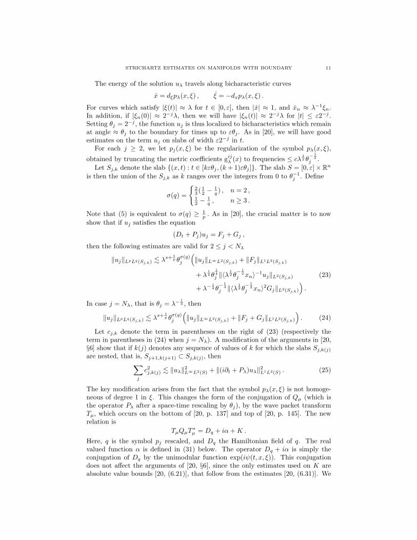
The energy of the solution uλ travels along bicharacteristic curves
x = dξpλ(x, ξ) , ξ = −dxpλ(x, ξ) .
For curves which satisfy |ξ(t)| ≈ λ for t ∈ [0, ε], then |x| ≈ 1, and xn ≈ λ−1ξn.In addition, if |ξn(0)| ≈ 2−jλ, then we will have |ξn(t)| ≈ 2−jλ for |t| ≤ ε2−j .Setting θj = 2−j , the function uj is thus localized to bicharacteristics which remainat angle ≈ θj to the boundary for times up to εθj . As in [20], we will have goodestimates on the term uj on slabs of width ε2−j in t.
For each j ≥ 2, we let pj(x, ξ) be the regularization of the symbol pλ(x, ξ),
obtained by truncating the metric coefficients gijλ (x) to frequencies ≤ cλ 12 θ− 1
2j .
Let Sj,k denote the slab (x, t) : t ∈ [kεθj , (k+ 1)εθj ]. The slab S = [0, ε]×Rnis then the union of the Sj,k as k ranges over the integers from 0 to θ−1
j . Define
σ(q) =
23 ( 1
2 −1q ) , n = 2 ,
12 −
1q , n ≥ 3 .
Note that (5) is equivalent to σ(q) ≥ 1p . As in [20], the crucial matter is to now
show that if uj satisfies the equation
(Dt + Pj)uj = Fj +Gj ,
then the following estimates are valid for 2 ≤ j < Nλ
‖uj‖LpLq(Sj,k) . λs+ 1
p θσ(q)j
(‖uj‖L∞L2(Sj,k) + ‖Fj‖L1L2(Sj,k)
+ λ14 θ
14j ‖〈λ
12 θ− 1
2j xn〉−1uj‖L2(Sj,k) (23)
+ λ−14 θ− 1
4j ‖〈λ
12 θ− 1
2j xn〉2Gj‖L2(Sj,k)
).
In case j = Nλ, that is θj = λ−13 , then
‖uj‖LpLq(Sj,k) . λs+ 1
p θσ(q)j
(‖uj‖L∞L2(Sj,k) + ‖Fj +Gj‖L1L2(Sj,k)
). (24)
Let cj,k denote the term in parentheses on the right of (23) (respectively theterm in parentheses in (24) when j = Nλ). A modification of the arguments in [20,§6] show that if k(j) denotes any sequence of values of k for which the slabs Sj,k(j)
are nested, that is, Sj+1,k(j+1) ⊂ Sj,k(j), then∑j
c2j,k(j) . ‖uλ‖2L∞L2(S) + ‖(i∂t + Pλ)uλ‖2L1L2(S) . (25)
The key modification arises from the fact that the symbol pλ(x, ξ) is not homoge-neous of degree 1 in ξ. This changes the form of the conjugation of Qµ (which isthe operator Pλ after a space-time rescaling by θj), by the wave packet transformTµ, which occurs on the bottom of [20, p. 137] and top of [20, p. 145]. The newrelation is
TµQµT∗µ = Dq + iα+K .
Here, q is the symbol pj rescaled, and Dq the Hamiltonian field of q. The realvalued function α is defined in (31) below. The operator Dq + iα is simply theconjugation of Dq by the unimodular function exp(iψ(t, x, ξ)). This conjugationdoes not affect the arguments of [20, §6], since the only estimates used on K areabsolute value bounds [20, (6.21)], that follow from the estimates [20, (6.31)]. We

12 MATTHEW D. BLAIR, HART F. SMITH, AND CHRIS D. SOGGE
also note that the estimates in [20] use (i∂t + Pλ)uλ ∈ L2L2(S), but as noted afterTheorem 2.3 above this is unimportant.
The estimates of Theorem 2.3 will then follow from (23)-(24) and the branchingargument on [20, p. 118].
In the proof of (23)-(24), we will from now on work with a fixed j, and willabbreviate θj = θ. We work with an angle-dependent rescaled uj , setting
u(t, x) = uj(θjt, θjx) , F (t, x) = θjFj(θjt, θjx) , G(t, x) = θjGj(θjt, θjx) ,
and q(x, ξ) = θjPj(θjx, θ−1j ξ). Set µ = λθj , so that q(x, ξ) ≈ µ when |ξ| ≈ µ.
Additionally, if |ξ| ≈ µ, then q(x, ξ) satisfies the following estimates; see [20, (4.1)].
|∂βx∂αξ q(x, ξ)| .
µ1−|α| , if |β| = 0 ,
c0(
1 + µ(|β|−1)/2θj〈µ12xn〉−N
)µ1−|α| , if |β| ≥ 1 .
(26)
We then have
Dtu− q(x,D)u = F +G ,
and the frequency localization condition holds
supp(u(t, ·)) ⊂
|ξ′| ∈ [ 1
4µ, 4µ] , |ξn| ∈ [ 14µθ, 2µθ] , θ > µ−
12 ,
|ξ′| ∈ [ 14µ, 4µ] , |ξn| ≤ µ
12 , θ = µ−
12 .
After translation in time, the estimates (23) reduce to showing that, over the slabS = [0, ε]× Rn ,
‖u‖LpLq(S) . µs+ 1
p θσ(q)(‖u‖L∞L2(S) + ‖F‖L1L2(S)
+ µ14 θ
12 ‖〈µ 1
2xn〉−1u‖L2(S) (27)
+ µ−14 θ−
12 ‖〈µ 1
2xn〉2G‖L2(S)
).
The estimates in (24) reduce to showing that, for θ = µ−12 ,
‖u‖LpLq(S) . µs+ 1
p θσ(q)(‖u‖L∞L2(S) + ‖F +G‖L1L2(S)
). (28)
To establish the inequalities (27) and (28), we use a wave packet transform toconstruct a suitable representation of u. Define the linear operator Tµ on Schwartzclass functions by
(Tµf)(x, ξ) = µn4
∫e−i〈ξ,y−x〉g(µ
12 (y − x))f(y) dy ,
where we fix g a radial Schwartz class function, with g supported in a ball of smallradius c. Taking ‖g‖L2(Rn) = (2π)−
n2 , it holds that T ∗µTµ = I and ‖Tµf‖L2(R2n
x,ξ)=
‖f‖L2(Rny ). We set
u(t, x, ξ) = (Tµu(t, ·))(x, ξ) .By Lemma 4.4 of [20], we may write(
∂t − dξq(x, ξ) · dx + dxq(x, ξ) · dξ + iq(x, ξ)− iξ · dξq(x, ξ))u(t, x, ξ)
= F (t, x, ξ) + G(t, x, ξ) , (29)
where, over S = [0, ε]× R2nx,ξ, the quantity
‖F‖L1L2(S) + µ−14 θ−
12 ‖〈µ 1
2xn〉2G‖L2(S)

STRICHARTZ ESTIMATES ON MANIFOLDS WITH BOUNDARY 13
is bounded by the right hand side of (27) when θ > µ−12 , and the quantity
‖F + G‖L1L2(S)
is bounded by the right hand side of (28) when θ = µ−12 . The proof of this lemma
relies only on the bounds (26), and thus applies in our situation. Also, given the
compact support of g, it can be seen that the ξ support of u, F , G is contained ina set where |ξ′| ≈ µ and ξn ≈ θµ (or |ξn| . µ
12 when θ = µ−
12 ).
Let Θr,t(x, ξ) denote the canonical transformation on R2nx,ξ = T ∗(Rnx) generated
by the Hamiltonian flow of q(x, ξ). That is, Θr,t(x, ξ) is the time r solution of
x = dξq(x, ξ′) , ξ = −dxq(x, ξ) , (30)
with initial conditions (x(t), ξ(t)) = (x, ξ) . Since q(x, ξ) is independent of time,Θr,t = Θr−t,0 . Also define
α(x, ξ) = q(x, ξ)− ξ · dξq(x, ξ) , ψ(t, x, ξ) =
∫ t
0
α(Θs,t(x, ξ)) ds . (31)
It follows by time independence of q that∫ trα(Θs,t(x, ξ)) ds = ψ(t− r, x, ξ) .
Equation (29) above allows us to write
u(t, x, ξ) = e−iψ(t,x,ξ)u(0,Θ0,t(x, ξ))
+
∫ t
0
e−iψ(t−r,x,ξ)(F (r,Θr,t(x, ξ)) + G(r,Θr,t(x, ξ))
)dr .
In the next section we will establish the following estimates for solutions to thehomogeneous flow equation,
Theorem 3.1. Suppose f ∈ L2(R2nx,ξ) is supported in a set of the form
|ξ′| ≈ µ , |ξn| ≈ µθ , θ > µ−12 ,
|ξ′| ≈ µ , |ξn| ≤ µ12 , θ = µ−
12 .
(32)
Define Wf(t, x) = T ∗µ[e−iψ(t,·)(f Θ0,t)
](x) . Then the following estimate holds for
s ≥ 0, p > 2, and q <∞ satisfying (5) and (7),
‖Wf‖LpLq(S) . µs+ 1
p θσ(q)‖f‖L2(R2n) . (33)
For f ∈ L2(R2nx,ξ) supported where |ξ′| ≤ µ, |ξn| ≈ µ, estimate (33) holds with θ = 1,
for s ≥ 0, p > 2, and q <∞ satisfying (7).
Since T ∗µTµ = I , it follows by the preceeding steps and variation of parameters
that this implies the estimates (28), as well as the estimates (27) in case G ≡ 0.
The reduction of the estimates (27) to Theorem 3.1 for G 6= 0 requires the V 2q
spaces introduced by Koch and Tataru [16], and follows exactly the arguments on[20, p. 124–126]. The key fact used in that proof about the Hamiltonian flow of qis that xn ≈ θ on the support of u(t, x, ξ), which holds in our case.
14 MATTHEW D. BLAIR, HART F. SMITH, AND CHRIS D. SOGGE
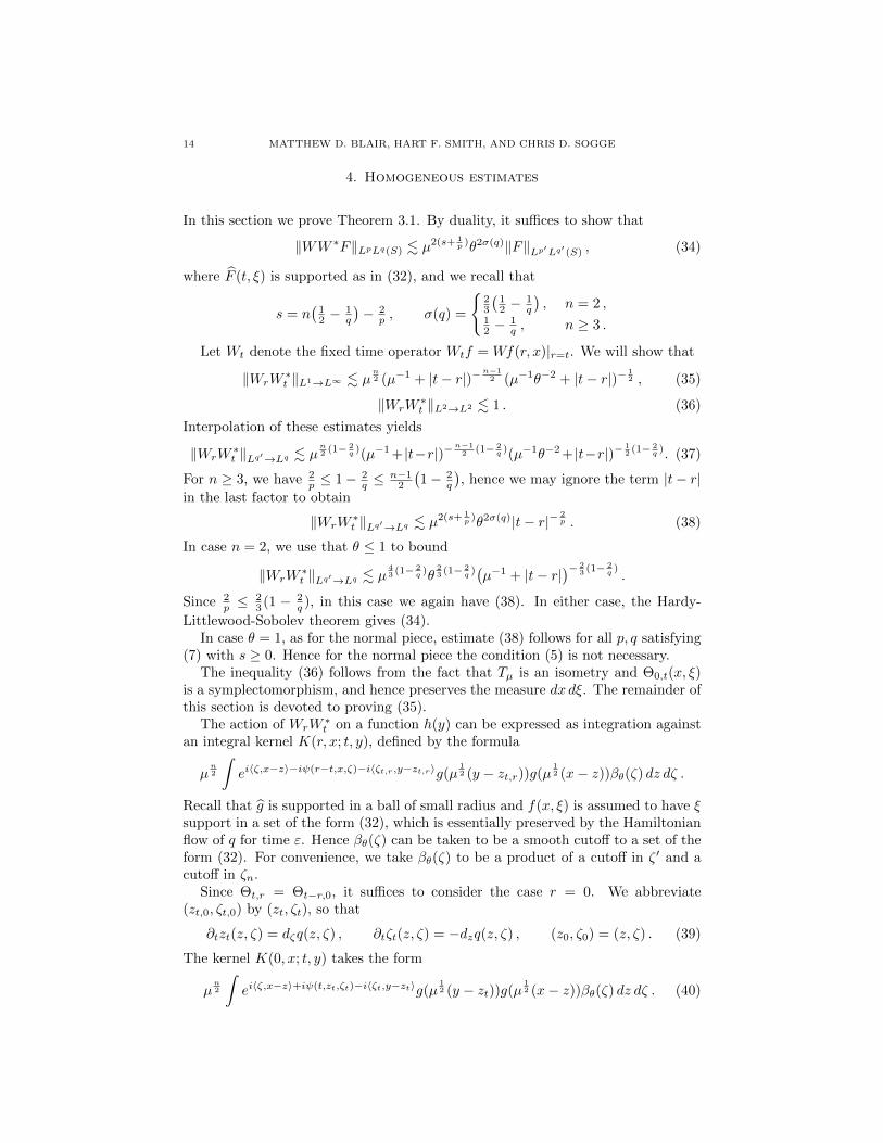
4. Homogeneous estimates
In this section we prove Theorem 3.1. By duality, it suffices to show that
‖WW ∗F‖LpLq(S) . µ2(s+ 1
p )θ2σ(q)‖F‖Lp′Lq′ (S) , (34)
where F (t, ξ) is supported as in (32), and we recall that
s = n(
12 −
1q
)− 2
p , σ(q) =
23
(12 −
1q
), n = 2 ,
12 −
1q , n ≥ 3 .
Let Wt denote the fixed time operator Wtf = Wf(r, x)|r=t. We will show that
‖WrW∗t ‖L1→L∞ . µ
n2 (µ−1 + |t− r|)−
n−12 (µ−1θ−2 + |t− r|)− 1
2 , (35)
‖WrW∗t ‖L2→L2 . 1 . (36)
Interpolation of these estimates yields
‖WrW∗t ‖Lq′→Lq . µ
n2 (1− 2
q )(µ−1 + |t−r|)−n−12 (1− 2
q )(µ−1θ−2 + |t−r|)−12 (1− 2
q ). (37)
For n ≥ 3, we have 2p ≤ 1− 2
q ≤n−1
2
(1− 2
q
), hence we may ignore the term |t− r|
in the last factor to obtain
‖WrW∗t ‖Lq′→Lq . µ
2(s+ 1p )θ2σ(q)|t− r|−
2p . (38)
In case n = 2, we use that θ ≤ 1 to bound
‖WrW∗t ‖Lq′→Lq . µ
43 (1− 2
q )θ23 (1− 2
q )(µ−1 + |t− r|
)− 23 (1− 2
q ).
Since 2p ≤
23 (1 − 2
q ), in this case we again have (38). In either case, the Hardy-
Littlewood-Sobolev theorem gives (34).In case θ = 1, as for the normal piece, estimate (38) follows for all p, q satisfying
(7) with s ≥ 0. Hence for the normal piece the condition (5) is not necessary.The inequality (36) follows from the fact that Tµ is an isometry and Θ0,t(x, ξ)
is a symplectomorphism, and hence preserves the measure dx dξ. The remainder ofthis section is devoted to proving (35).
The action of WrW∗t on a function h(y) can be expressed as integration against
an integral kernel K(r, x; t, y), defined by the formula
µn2
∫ei〈ζ,x−z〉−iψ(r−t,x,ζ)−i〈ζt,r,y−zt,r〉g(µ
12 (y − zt,r))g(µ
12 (x− z))βθ(ζ) dz dζ .
Recall that g is supported in a ball of small radius and f(x, ξ) is assumed to have ξsupport in a set of the form (32), which is essentially preserved by the Hamiltonianflow of q for time ε. Hence βθ(ζ) can be taken to be a smooth cutoff to a set of theform (32). For convenience, we take βθ(ζ) to be a product of a cutoff in ζ ′ and acutoff in ζn.
Since Θt,r = Θt−r,0, it suffices to consider the case r = 0. We abbreviate(zt,0, ζt,0) by (zt, ζt), so that
∂tzt(z, ζ) = dζq(z, ζ) , ∂tζt(z, ζ) = −dzq(z, ζ) , (z0, ζ0) = (z, ζ) . (39)
The kernel K(0, x; t, y) takes the form
µn2
∫ei〈ζ,x−z〉+iψ(t,zt,ζt)−i〈ζt,y−zt〉g(µ
12 (y − zt))g(µ
12 (x− z))βθ(ζ) dz dζ . (40)

STRICHARTZ ESTIMATES ON MANIFOLDS WITH BOUNDARY 15
Theorem 4.1. Suppose (zt(z, ζ), ζt(z, ζ)) are defined by (39) and dz, dζ denote the
z and ζ gradient operators. Then if |ζ| ≈ µ, and ζn ≈ µθ, or |ζn| . µ12 in the case
θ = µ−12 , the following bounds hold,
|dzzt − I| . t , |dζzt| . µ−1t , (41)
|dζζt − I| . t , |dzζt| . µ ,as well as the more precise estimate∣∣∣∣dζzt − ∫ t
0
d2ζq(zs, ζs) ds
∣∣∣∣ . µ−1t2 . (42)
Furthermore, for second order derivatives we have
|d2zzt| . 〈µ
12 t〉 , |d2
zζt| . µ32 , (43)
|dzdζzt| . µ−1t〈µ 12 t〉 , |dzdζζt| . 〈µ
12 t〉 . (44)
Finally, for l ≥ 2 we have
µl|dlζzt|+ µl−1|dlζζt| . t〈µ12 t〉l−1 . (45)
Proof. The proof is a rescaled version of Theorem 5.1 and Corollary 5.2 of [20], butfor completeness we sketch the details here.
Differentiating Hamilton’s equations one obtains
∂t
[dztdζt
]= M(zt, ζt)
[dztdζt
], M(z, ζ) =
[dzdζq dζdζq−dzdzq −dζdzq
].
To keep all terms of the same order in µ, we take the following rescaled equation,
∂t
[dzzt µdζzt
µ−1dzζt dζζt
]= Mµ(zt, ζt)
[dzzt µdζzt
µ−1dzζt dζζt
], (46)
where
Mµ(z, ζ) =
[dzdζq µ dζdζq
−µ−1dzdzq − dζdzq
].
The key estimate on Mµ is that, for j + k = 2 ,
∫ t
0
|(djzdkζq)(zs, ζs)| ds .
µ−1t , if k = 2 ,
t , if j = k = 1 ,
µ , if j = 2 .
(47)
This follows from (26) and the property |(∂tzt)n| ≈ θ for t ∈ [0, ε], when θ > µ−12 .
When θ = µ−12 , the estimates (26) are uniform over |β| ≤ 2, and (47) also follows.
Gronwall’s lemma now gives that
|dzzt|+ µ |dζzt|+ µ−1|dzζt|+ |dζζt| . 1 .
Integrating (46) and using (47) yields (41). The estimate |dζζt − I| . t can thenbe substituted in the integral equation for ∂ζzt to give (42).
To show the higher order estimates (45), we work with the equation
∂t
[µldlζztµl−1dlζζt
]= Mµ(zt, ζt)
[µldlζztµl−1dlζζt
]+
[E1(t)E2(t)
].
Here E1(t) is a sum of terms of the form
(µkdjzdk+1ζ q)(zt, ζt)(µ
l1d l1ζ zt) . . . (µljd
ljζ zt)(µ
lj+1−1dlj+1
ζ ζt) . . . (µlj+k−1d
lj+kζ ζt).
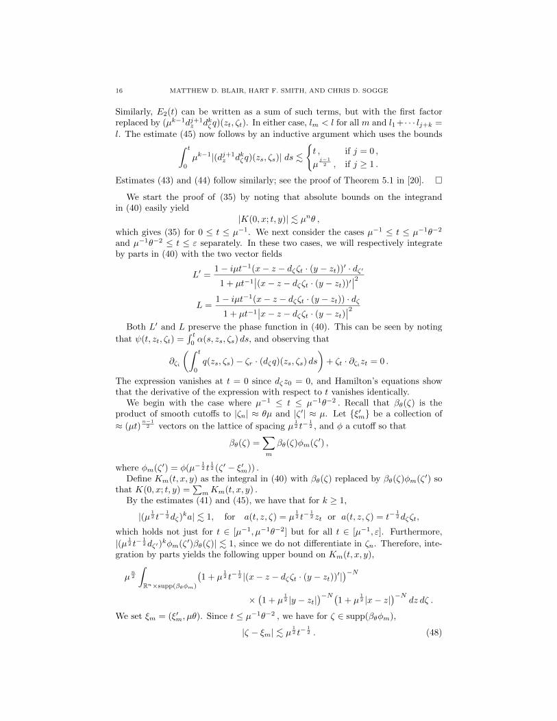
16 MATTHEW D. BLAIR, HART F. SMITH, AND CHRIS D. SOGGE
Similarly, E2(t) can be written as a sum of such terms, but with the first factorreplaced by (µk−1dj+1
z dkζq)(zt, ζt). In either case, lm < l for all m and l1 + · · · lj+k =
l. The estimate (45) now follows by an inductive argument which uses the bounds∫ t
0
µk−1|(dj+1z dkζq)(zs, ζs)| ds .
t , if j = 0 ,
µj−12 , if j ≥ 1 .
Estimates (43) and (44) follow similarly; see the proof of Theorem 5.1 in [20].
We start the proof of (35) by noting that absolute bounds on the integrandin (40) easily yield
|K(0, x; t, y)| . µnθ ,which gives (35) for 0 ≤ t ≤ µ−1. We next consider the cases µ−1 ≤ t ≤ µ−1θ−2
and µ−1θ−2 ≤ t ≤ ε separately. In these two cases, we will respectively integrateby parts in (40) with the two vector fields
L′ =1− iµt−1(x− z − dζζt · (y − zt))′ · dζ′
1 + µt−1∣∣(x− z − dζζt · (y − zt))′∣∣2
L =1− iµt−1(x− z − dζζt · (y − zt)) · dζ
1 + µt−1∣∣x− z − dζζt · (y − zt)∣∣2
Both L′ and L preserve the phase function in (40). This can be seen by noting
that ψ(t, zt, ζt) =∫ t
0α(s, zs, ζs) ds, and observing that
∂ζi
(∫ t
0
q(zs, ζs)− ζr · (dζq)(zs, ζs) ds)
+ ζt · ∂ζizt = 0 .
The expression vanishes at t = 0 since dζz0 = 0, and Hamilton’s equations showthat the derivative of the expression with respect to t vanishes identically.
We begin with the case where µ−1 ≤ t ≤ µ−1θ−2 . Recall that βθ(ζ) is theproduct of smooth cutoffs to |ζn| ≈ θµ and |ζ ′| ≈ µ. Let ξ′m be a collection of
≈ (µt)n−12 vectors on the lattice of spacing µ
12 t−
12 , and φ a cutoff so that
βθ(ζ) =∑m
βθ(ζ)φm(ζ ′) ,
where φm(ζ ′) = φ(µ−12 t
12 (ζ ′ − ξ′m)) .
Define Km(t, x, y) as the integral in (40) with βθ(ζ) replaced by βθ(ζ)φm(ζ ′) sothat K(0, x; t, y) =
∑mKm(t, x, y) .
By the estimates (41) and (45), we have that for k ≥ 1,
|(µ 12 t−
12 dζ)
ka| . 1, for a(t, z, ζ) = µ12 t−
12 zt or a(t, z, ζ) = t−
12 dζζt,
which holds not just for t ∈ [µ−1, µ−1θ−2] but for all t ∈ [µ−1, ε]. Furthermore,
|(µ 12 t−
12 dζ′)
kφm(ζ ′)βθ(ζ)| . 1, since we do not differentiate in ζn. Therefore, inte-gration by parts yields the following upper bound on Km(t, x, y),
µn2
∫Rn×supp(βθφm)
(1 + µ
12 t−
12 |(x− z − dζζt · (y − zt))′|
)−N×(1 + µ
12 |y − zt|
)−N(1 + µ
12 |x− z|
)−Ndz dζ .
We set ξm = (ξ′m, µθ). Since t ≤ µ−1θ−2 , we have for ζ ∈ supp(βθφm),
|ζ − ξm| . µ12 t−
12 . (48)

STRICHARTZ ESTIMATES ON MANIFOLDS WITH BOUNDARY 17
Recall that zt = zt(z, ζ) is the spatial component of Θt,0(z, ζ). We let xmt =zt(x, ξm) denote the spatial component of Θt,0(x, ξm). We then claim that, forζ ∈ supp(βθφm),
µ12 t−
12 |x− z − dζζt · (xmt − zt)| . 1 + µ |x− z|2. (49)
Assuming this for the moment, we dominate the integrand for Km by(1 + µ
12 t−
12 |(dζζt · (y − xmt ))′|
)−N(1 + µ
12 |y − zt|
)−N(1 + µ
12 |x− z|
)−N. (50)
By (41) and (48), we have |xmt − zt| . µ−12 t
12 + |x− z|. Thus, since |dζζt− I| . |t|,
we conclude that
µ12 t−
12 |(dζζt · (y − xmt ))′| & µ 1
2 t−12 |(y − xmt )′| − µ 1
2 t12 |y − xmt |
& µ12 t−
12 |(y − xmt )′| − µ 1
2 t12
(|y − zt|+ |x− z|
)− |t| .
The negative terms on the right here are small compared to the last two termsin (50). Therefore, we have
|Km(t, x, y)| . µn+12 θ t−
n−12
(1 + µ
12 t−
12 |(y − xmt )′|
)−N,
which follows by observing the rapid decay of the integrand in z, and that the
volume of supp(φmβθ) is comparable to µn+12 θ t−
n−12 .
We next observe that, by (42) and the estimate∥∥d2ζq(z, ζ)− 2µ−1I
∥∥ . µ−1‖gij − δij‖ . c0µ−1 ,
we have that
|(xmt − xlt)− 2µ−1t(ξm − ξl)| µ−1t |ξm − ξl| ,and since |ξm − ξl| = |ξ′m − ξ′l|, we conclude that
µ12 t−
12 |(xmt − xlt)′| ≈ µ−
12 t
12 |ξ′m − ξ′l| . (51)
Since the ξ′m lie on a µ12 t−
12 spaced lattice, we may sum over m to obtain
|K(0, x; t, y)| . µn+12 θ t−
n−12
∑m
(1 + µ
12 t−
12 |(y − xmt )′|
)−N. µ
n+12 θ t−
n−12 ,
yielding (35) for µ−1 ≤ t ≤ µ−1θ−2.To handle the case µ−1θ−2 ≤ t ≤ ε , we modify the above proof by considering
an O(µn2 t
n2 ) collection of vectors ξm in a µ
12 t−
12 spaced lattice in Rn, and an
associated partition φm(ζ) = φ(µ−12 t
12 (ζ − ξm)), satisfying
βθ(ζ) =∑m
βθ(ζ)φm(ζ) .
We now define Km(t, x, y) as the integral in (40) with βθ(ζ) replaced by βθ(ζ)φm(ζ).
Here, since µ12 t−
12 ≤ µθ, we have
|(µ 12 t−
12 dζ)
kφm(ζ)βθ(ζ)| . 1 .
Integrating by parts with respect to the vector field L now shows that Km(t, x, y)is bounded by
µn2
∫Rn×supp(βθφm)
(1 + µ
12 t−
12 |x− z − dζζt · (y − zt)|
)−N×(1 + µ
12 |y − zt|
)−N(1 + µ
12 |x− z|
)−Ndz dζ .

18 MATTHEW D. BLAIR, HART F. SMITH, AND CHRIS D. SOGGE
Using (49), which holds for any t ∈ [µ−1, ε] , we proceed as before and concludethat
|Km(t, x, y)| . µn2 t−n2(1 + µ
12 t−
12 |y − xmt |
)−N.
The n-dimensional analogue of (51) is valid here, so we may use the spacing of theξm as above to sum over m and obtain (35) for t > µ−1θ−2, that is,
|K(0, x; t, y)| . µn2 t−n2 .Returning to (49), we first observe that by estimating the Taylor remainder
using (43)–(45) and (48), the following holds
µ12 t−
12 |xmt − zt − (dzzt)(x− z)− (dζzt)(ξm − ζ)| . 1 + µ|x− z|2 .
Furthermore by (41) and (48), we have
µ12 t−
12 |(dζzt)(ξm − ζ)| . 1 .
From the fact that (z, ζ)→ (zt, ζt) is a symplectic transformation, we have
∂ζiζt · ∂zjzt − ∂ζizt · ∂zjζt = δij ,
where · pairs the zt and ζt indices. Lastly, by (41),
µ12 t−
12 |dζzt| |dzζt| |x− z| . µ
12 t
12 |x− z| ≤ µ 1
2 |x− z| .These facts now combine to yield (49).
5. Applications to semilinear Schrodinger equations on exteriordomains
In this section, we assume that Ω = R3 \ K is the domain exterior to a smoothnon-trapping obstacle K (or any exterior domain where (4) holds). We consider theinitial value problem for the following family of semilinear Schrodinger equationsin 3 + 1 dimensions,
i∂tu+ ∆u± |u|r−1u = 0 , u(0, x) = f(x) , (52)
satisfying homogeneous Dirichlet or Neumann boundary conditions
u(t, x)∣∣∂Ω
= 0 , or ∂νu(t, x)∣∣∂Ω
= 0 . (53)
Precisely, by a solution to (52)-(53), we understand that, with F (u) = ±|u|r−1u,and u(t) denoting the function u(t, ·),
u(t) = eit∆f + i
∫ t
0
ei(t−s)∆ F (u(s)) ds , (54)
where exp(it∆) is the unitary Schrodinger propagator defined using the Dirichletor Neumann spectral resolution. Defocusing means that F (u) = −|u|r−1u. Sincewe will work with H1 data, the boundary conditions required of the initial datain the Dirichlet case are that f vanish on ∂Ω; in the Neumann case the boundaryconditions are void, i.e. f is the restriction to Ω of a general function in H1(R3).
Planchon and Vega showed in [17] that, for 1 < r < 5 and defocusing nonlinear-ities, one has global existence of solutions to the Dirichlet problem for f ∈ H1. Acrucial ingredient in their proof was the estimate in Theorem 1.1 with p = q = 4and s = 1
4 . They combined this with local smoothing estimates near the boundary
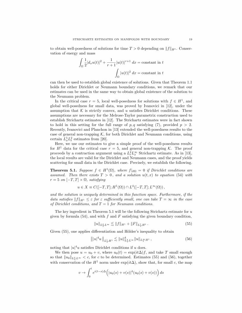
STRICHARTZ ESTIMATES ON MANIFOLDS WITH BOUNDARY 19
to obtain well-posedness of solutions for time T > 0 depending on ‖f‖H1 . Conser-vation of energy and mass∫
Ω
1
2|dxu(t)|2 +
1
r + 1|u(t)|r+1 dx = constant in t∫Ω
|u(t)|2 dx = constant in t
can then be used to establish global existence of solutions. Given that Theorem 1.1holds for either Dirichlet or Neumann boundary conditions, we remark that ourestimates can be used in the same way to obtain global existence of the solution tothe Neumann problem.
In the critical case r = 5, local well-posedness for solutions with f ∈ H1, andglobal well-posedness for small data, was proved by Ivanovici in [12], under theassumption that K is strictly convex, and u satisfies Dirichlet conditions. Theseassumptions are necessary for the Melrose-Taylor parametrix construction used toestablish Strichartz estimates in [12]. The Strichartz estimates were in fact shownto hold in this setting for the full range of p, q satisfying (7), provided p > 2.Recently, Ivanovici and Planchon in [13] extended the well-posedness results to thecase of general non-trapping K, for both Dirichlet and Neumann conditions, usingcertain L5
xL2t estimates from [20].
Here, we use our estimates to give a simple proof of the well-posedness resultsfor H1 data for the critical case r = 5, and general non-trapping K. The proofproceeds by a contraction argument using a L4
tL∞x Strichartz estimate. As in [13],
the local results are valid for the Dirichlet and Neumann cases, and the proof yieldsscattering for small data in the Dirichlet case. Precisely, we establish the following.
Theorem 5.1. Suppose f ∈ H1(Ω), where f |∂Ω = 0 if Dirichlet conditions areassumed. Then there exists T > 0 , and a solution u(t, x) to equation (54) withr = 5 on [−T, T ]× Ω, satisfying
u ∈ X ≡ C([−T, T ];H1(Ω)) ∩ L4([−T, T ];L∞(Ω)) ,
and the solution is uniquely determined in this function space. Furthermore, if thedata satisfies ‖f‖H1 ≤ ε for ε sufficiently small, one can take T = ∞ in the caseof Dirichlet conditions, and T = 1 for Neumann conditions.
The key ingredient in Theorem 5.1 will be the following Strichartz estimate for ugiven by formula (54), and with f and F satisfying the given boundary condition,
‖u‖L4TL∞ . ‖f‖H1 + ‖F‖L1
TH1 . (55)
Given (55), one applies differentiation and Holder’s inequality to obtain∥∥|u|4u∥∥L1TH
1 . ‖u‖4L4TL∞‖u‖L∞T H1 , (56)
noting that |u|4u satisfies Dirichlet conditions if u does.We then pose u = u0 + v, where u0(t) = exp(it∆)f , and take T small enough
so that ‖u0‖L4TL∞ < c, for c to be determined. Estimates (55) and (56), together
with conservation of the H1 norm under exp(it∆), show that, for small c, the map
v →∫ t
0
ei(t−s)∆(|u0(s) + v(s)|4(u0(s) + v(s))
)ds

20 MATTHEW D. BLAIR, HART F. SMITH, AND CHRIS D. SOGGE
maps the ball ‖v‖X ≤ c into itself. Similar analysis shows that the map is in facta contraction on this ball, for small c, yielding a fixed point v. If ‖f‖H1 ≤ ε, thenone can take T =∞ for the Dirichlet case, or T = 1 for the Neumann case.
For defocusing Neumann, energy and mass conservation then yield global exis-tence. For small norm Dirichlet data, the proof implies |u|4u ∈ L1(R, H1(Ω)). Thisyields that such solutions scatter, in the sense that they asymptotically approachin the H1 norm a solution to the homogeneous equation.
In establishing (55), it suffices by the Duhamel principle to consider F = 0. Theproof of (55) will be obtained from the following cases of Theorem 1.1,
‖u‖L12L9 . ‖f‖H1 , ‖u‖L3L9 . ‖f‖H
12.
The second estimate could be expressed as controlling the L3W12 ,9 norm of u in
terms of ‖f‖H1 , and we would then apply a fractional Gagliardo-Nirenberg inequal-
ity to control ‖u(t)‖L∞ by interpolating L9 and W12 ,9. We can avoid dealing with
fractional Lp Sobolev spaces on exterior domains, however, by carrying out thesame steps more directly. The interpolation we will use is the following.
Lemma 5.2. Suppose that α1, α2 > 0, and u =∑∞j=0 uj, where
‖uj‖L∞ ≤ min(
2−jα1ρ1 , 2jα2ρ2
).
Then
‖u‖L∞ ≤ Cα1,α2ρα2
α1+α21 ρ
α1α1+α22 .
Proof. The proof follows by summing the smaller of the bounds, i.e. separating the
sum depending on whether 2j ≥ (ρ1/ρ2)1
α1+α2 or not. The bound applies with
Cα1,α2 =2α1
2α1 − 1+
2α2
2α2 − 1.
We next take a Littlewood-Paley decomposition of the initial data
f =
∞∑j=1
β(2−2jH)f + β0(H)f ,
where β(s) is supported in the interval s ∈ [ 12 ,
92 ], and 1 = β0(s) +
∑∞j=0 β(2−2js)
for s ≥ 0. Here, H denotes −∆ with either Dirichlet or Neumann conditions. Set
fj = e2−2jHβ(2−2jH)f , f0 = eHβ0(H)f .
By the spectral localization,∞∑j=0
‖fj‖2H1 . ‖f‖2H1 ,
and we may write u(t) =∑∞j=0 uj(t) , where
uj(t) = e−2−2jHe−itHfj , u0(t) = e−He−itHf0 .
By the ultracontractivity estimate for H on exterior domains (see Theorem 2.4.2and the ensuing comments in [7], where µ = 3 in our case), we can bound
‖uj(t)‖L∞ . 2j3 ‖e−itHfj‖L9 .

STRICHARTZ ESTIMATES ON MANIFOLDS WITH BOUNDARY 21
Together with the case (p, q, s) = (3, 9, 12 ) of Theorem 1.1, we have
‖2−j3uj‖L3L∞ . ‖e−itHfj‖L3L9 . ‖fj‖
H12≤ 2−
j2 ‖fj‖H1 ,
which we combine with Minkowski’s inequality to yield(∫ ( ∞∑j=0
‖2j6uj(t)‖2L∞
) 32
dt
) 13
≤( ∞∑j=0
‖2j6uj‖2L3L∞
) 12
. ‖f‖2H1 .
In particular,
supj
2j6 ‖uj(t)‖L∞ ≤ ρ1(t) , ‖ρ1‖L3 . ‖f‖H1 .
Similar considerations, using the case (p, q, s) = (12, 9, 1) of Theorem 1.1, yield
supj
2−j3 ‖uj(t)‖L∞ ≤ ρ2(t) , ‖ρ2‖L12 . ‖f‖H1 .
Lemma 5.2 now applies to give the bound
‖u(t)‖L∞ . ρ1(t)23 ρ2(t)
13 .
Applying Holder’s inequality with the dual indices ( 98 , 9) now yields
‖u‖4L4L∞ .∫ρ1(t)
83 ρ2(t)
43 dt . ‖ρ1‖
83
L3 ‖ρ2‖43
L12 . ‖f‖4H1 .
6. Applications to semilinear Schrodinger equations on compactmanifolds
In this section we consider a compact 3-dimensional Riemannian manifold Ω withboundary. We assume G : [0,∞)→ R is bounded below, with G(0) = 0, and that
|G′(r)|+ r |G′′(r)| . 〈r〉 15 . (57)
We set F (u) = G′(|u|2)u, so that
|F (u)| ≤ 〈u〉2/5|u| , |duF (u)| ≤ 〈u〉2/5 .We prove existence, uniqueness, and energy conservation, for initial data u(t0) ∈H1(Ω), to the semilinear Schrodinger equation
i∂tu+ ∆u = F (u) , u|t=t0 = u(t0) , (58)
satisfying homogeneous Dirichlet or Neumann boundary conditions (53). As above,by a solution to (58) we understand that its integral form holds,
u(t) = ei(t−t0)∆
(u(t0)− i
∫ t
t0
e−i(s−t0)∆F (u(s)) ds
). (59)
This formulation is seen to be independent of t0; that is, if u solves (59) on aninterval for some t0 then it solves the same equation for all t0 in that interval.
The key estimates we use involve values of (p, q) which do not satisfy (5). Inthis case, the method of proof yields estimates with a loss of derivatives relativeto the scale invariant value of s from (7). In particular, the following analogue ofTheorem 2.1 loses 1
q derivatives relative to the case of manifolds without boundary
considered in [5]. Additionally, there are logarithmic losses due to the endpointp = 2 and q =∞.

22 MATTHEW D. BLAIR, HART F. SMITH, AND CHRIS D. SOGGE
Lemma 6.1. Let n = 3, and suppose that for all t, uλ(t, · ) is spectrally localizedfor −∆g to the range [ 1
4λ2, 4λ2]. Then the following estimate holds, uniformly for
6 ≤ q ≤ ∞, where Fλ = (i∂t + ∆g)uλ,
‖uλ‖L2λ−1L
q(Ω) ≤ Cλ12−
2q (log λ)2
(λ
12 ‖uλ‖L2
λ−1L2(Ω) + λ−
12 ‖Fλ‖L2
λ−1L2(Ω)
). (60)
Proof. We start by noting that the reduction of Theorem 2.1 to Theorem 2.3 holdswith uniform constant over q ≥ 6 with p = 2. In particular, in the handling of thenormal piece, q0 = 6 for p = 2, and s ≤ 1
2 in our estimates, so the use of Sobolevembedding works for that piece. Thus, (60) is a consequence of the estimate∥∥uλ‖L2
εLq ≤ Cλ1− 2
q (log λ)2(‖uλ‖L∞ε L2 + ‖(i∂t + Pλ)uλ‖L1
εL2
),
together with the following estimate, valid if uλ is localized to |ξn| ≥ 120 |ξ|,∥∥uλ‖L2
εLq ≤ Cλ1− 3
q (log λ)2(‖uλ‖L∞ε L2 + ‖(i∂t + Pλ)uλ‖L1
εL2
),
where Pλ is as in Theorem 2.3. These estimates in turn follows as a consequenceof the following analogue of (23)
‖uj‖L2Lq(Sj,k) ≤ Cλ1− 3q (log λ)
32 θ
12−
3q
j
(‖uj‖L∞L2(Sj,k) + ‖Fj‖L1L2(Sj,k)
+ λ14 θ
14j ‖〈λ
12 θ− 1
2j xn〉−1uj‖L2(Sj,k) (61)
+ λ−14 θ− 1
4j ‖〈λ
12 θ− 1
2j xn〉2Gj‖L2(Sj,k)
).
To see this, we note that for p = 2, the branching argument [20, p.118] requires
θ12j to converge, and the remaining term θ
− 3q
j is bounded by λ1q . The additional
loss of (log λ)12 here comes from the fact that there are ∼ log λ terms j in the
decomposition of uλ =∑j uj . We thus have, uniformly in q,
‖uλ‖L2εL
q . (log λ)12
∥∥(∑j
|uj |2) 1
2∥∥L2εL
q ,
and it is the norm on the right hand side that is controlled by the branchingargument.
The estimate (61) is scale invariant; scaling by θ reduces it to the followinganalogue of (27), for angularly localized u satisfying (Dt − q(x,D))u = F +G,
‖u‖L2Lq(S) . µ1− 3
q (logµ)32 θ
12−
3q
(‖u‖L∞L2(S) + ‖F‖L1L2(S)
+ µ14 θ
12 ‖〈µ 1
2xn〉−1u‖L2(S) (62)
+ µ−14 θ−
12 ‖〈µ 1
2xn〉2G‖L2(S)
),
where we used that logµ ≈ log λ.The reduction of (62) to homogeneous estimates, that is, bounds on the operator
W of (33), involves a loss of log µ due to the fact that p = 2. This comes from theuse of the V 2
q spaces introduced by Koch and Tataru [16], where the subscript qrefers to the Hamiltonian flow for q(x, ξ). In case p = 2, one needs to control the2-atomic norm U2
q of u, whereas V 2q ⊂ Upq only for p > 2. To proceed, we note that
in the atomic decomposition argument of [16, Lemma 6.4], we may truncate thesum u =
∑n vn to n . logµ, since the error is bounded in L∞L2 by µ−N , and its
contribution thus may be estimated in the desired norm using Sobolev embedding.

STRICHARTZ ESTIMATES ON MANIFOLDS WITH BOUNDARY 23
Each term vn is uniformly bounded in U2q , hence the U2
q norm of the truncated sumis . logµ.
We are thus reduced to establishing the following analogue of (33),
‖Wf‖L2Lq(S) ≤ Cµ1− 3q (logµ)
12 θ
12−
3q ‖f‖L2(R2n) . (63)
To establish (63), we consider WW ∗ as in the proof of Theorem 3.1. Takingn = 3 in (37), we note the following integral bound for 6 ≤ q ≤ ∞, µ and θ asabove,∫ 1
0
(µ−1 + t)−(1− 2q )(µ−1θ−2 + t)−
12 (1− 2
q ) dt ≤ Cµ32 (1− 2
q )−1(logµ)θ1− 6q ,
where C is uniformly bounded. The estimate (63) follows by Schur’s lemma.
We use Lemma 6.1 to deduce the following analogue of Lemma 3.6 of [5]. This
version is weaker, both in the logarithmic loss and the loss of λ1q , but is sufficient
for our purposes. From now on, we let uλ = β(λ−2H)u denote a Littlewood-Paleydecomposition of u, where λ = 2k and k ≥ 1. The term k = 0 contains the lowfrequency terms of u, and the bounds for this term will follow similarly to k = 1.
Lemma 6.2. Let u solve (59). Then there are C < ∞ and ε > 0 such that,uniformly for 6 ≤ q ≤ ∞, the following holds on any time interval [0, T ] withλ−1 ≤ T ≤ 1,
‖uλ‖L2([0,T ],Lq) ≤ Cλ−2q (log λ)2
(‖uλ‖L2([0,T ],H1) + λ−ε
⟨‖u‖L∞([0,T ],H1)
⟩7/5).
(64)
Proof. We divide [0, T ] into subintervals of length λ−1. We apply (60) on each suchsubinterval, and square sum over subintervals to obtain
‖uλ‖L2([0,T ],Lq) ≤ C λ−2q (log λ)2
(‖uλ‖L2([0,T ],H1) + ‖Fλ‖L2([0,T ],L2)
),
where Fλ = F (u)λ. We now take
α =2
5, r =
6
3 + α, ε = 3
(1
r− 1
2
)− 1 ,
and observe that
‖Fλ‖L∞L2 . λ−ε‖F‖L∞W 1,r
. λ−ε‖〈u〉α(|dxu|+ 〈u〉)‖L∞Lr
. λ−ε‖〈u〉‖αL∞L6‖(|dxu|+ 〈u〉)‖L∞L2
. λ−ε(1 + ‖u‖L∞H1
)α+1.
Sobolev embedding yields ‖u<T−1‖L2TL
q . T−12 ‖u‖L2
TH1 . ‖u‖L∞T H1 , where
u<T−1 denotes the sum of uλ over λ < T−1. Summing (64) over λ = 2−k, andusing Cauchy-Schwarz over k, we conclude that, with C uniform over q ≥ 6,
‖u‖L2([0,T ],Lq) ≤ C q52
(1 + ‖u‖L∞H1
)7/5. (65)

24 MATTHEW D. BLAIR, HART F. SMITH, AND CHRIS D. SOGGE
Suppose now that u satisfies (59) on a time interval [0, T ], where u(t0) ∈ H1(Ω).For sufficiently regular solutions u, we have the conservation laws∫
Ω
|u(t)|2 =
∫Ω
|u(t0)|2∫Ω
|dxu(t)|2g +G(|u(t)|2) =
∫Ω
|dxu(t0)|2g +G(|u(t0)|2)
(66)
In particular, since −C ≤ G(r) ≤ C〈r〉 65 , it follows that ‖u‖L∞([0,T ],H1) . 1 +‖u(t0)‖H1 , uniformly in T .
In the following proof, we assume a priori that u ∈ L∞H1 and prove uniquenessof such solutions. The existence of bounded energy solutions, and energy conserva-tion, is then proved by a weak-limit argument.
Theorem 6.3. For each data f ∈ H1(Ω), and all T > 0, there exists a uniquesolution u to the equation (59), subject to the condition u ∈ L∞([0, T ], H1(Ω)).Furthermore, the solution satisfies the conservation laws (66).
Proof. We start with the uniqueness of solutions. Since u ∈ L∞([0, T ], H1) itfollows by Sobolev embedding that F (u) ∈ L∞L2, so u ∈ C([0, T ], L2), and byinterpolation u ∈ C([0, T ], Hs) for all s < 1. Repeating this argument shows thatthe term in parentheses in (59) belongs to C1([0, T ], L2).
Let u and v be two solutions to (59), with u(0) = v(0). By unitarity of exp(it∆),
d
dt‖u(t)− v(t)‖2L2 =
d
dt
∥∥e−it∆(u(t)− v(t))∥∥2
L2
= 2 Im⟨F (u(t))− F (v(t)), u(t)− v(t)
⟩≤ C
∫Ω
(〈u(t)〉2/5 + 〈v(t)〉2/5
)|u(t)− v(t)|2
≤ C(1 + ‖u(t)‖L2q/5 + ‖v(t)‖L2q/5
) 25 ‖u(t)− v(t)‖2
L2q′
provided q ≥ 5/2. Since ‖u(t)− v(t)‖L6 ≤ C, we may interpolate to bound
‖u(t)− v(t)‖L2q′ ≤ C‖u(t)− v(t)‖1−32q
L2 .
Setting g(t) = ‖u(t)− v(t)‖2L2 , and noting g(0) = 0, we have upon integrating that
g(τ)32q ≤ C
q
∫ τ
0
(‖u(t)‖
25
L2q/5 + ‖v(t)‖25
L2q/5
)dt+
Cτ
q.
By Holder’s inequality and (65), for τ ∈ [0, T ]∫ τ
0
‖u(t)‖25
L2q/5 dt ≤ τ45 ‖u‖
25
L2([0,T ],L2q/5)≤ Cτ 4
5 q .
Consequently,
g(τ) ≤(Cτ
45 +
Cτ
q
) 2q3
which goes to 0 as q → ∞, provided τ is small depending on C. Repeating theargument yields uniqueness on [0, T ].
To establish existence and energy conservation for (59) with H1 data, we letGj(r) be a family of smooth, compactly supported real valued functions on [0,∞),
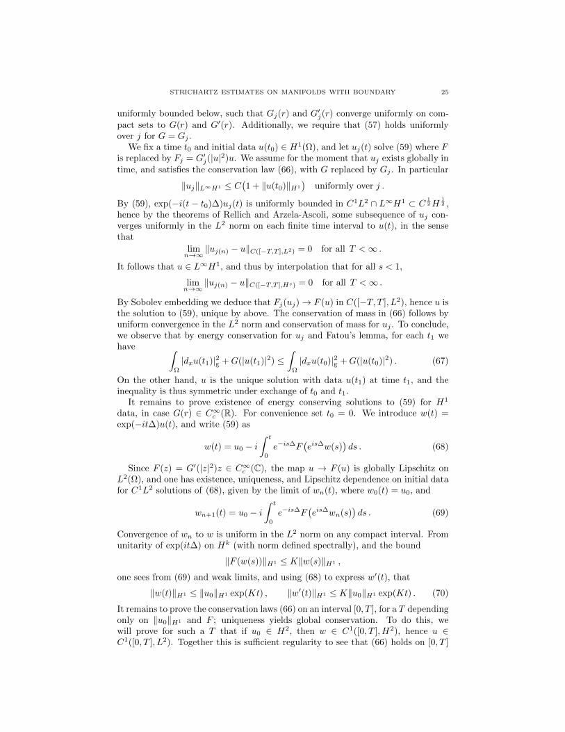
STRICHARTZ ESTIMATES ON MANIFOLDS WITH BOUNDARY 25
uniformly bounded below, such that Gj(r) and G′j(r) converge uniformly on com-pact sets to G(r) and G′(r). Additionally, we require that (57) holds uniformlyover j for G = Gj .
We fix a time t0 and initial data u(t0) ∈ H1(Ω), and let uj(t) solve (59) where Fis replaced by Fj = G′j(|u|2)u. We assume for the moment that uj exists globally intime, and satisfies the conservation law (66), with G replaced by Gj . In particular
‖uj‖L∞H1 ≤ C(1 + ‖u(t0)‖H1
)uniformly over j .
By (59), exp(−i(t − t0)∆)uj(t) is uniformly bounded in C1L2 ∩ L∞H1 ⊂ C12H
12 ,
hence by the theorems of Rellich and Arzela-Ascoli, some subsequence of uj con-verges uniformly in the L2 norm on each finite time interval to u(t), in the sensethat
limn→∞
‖uj(n) − u‖C([−T,T ],L2) = 0 for all T <∞ .
It follows that u ∈ L∞H1, and thus by interpolation that for all s < 1,
limn→∞
‖uj(n) − u‖C([−T,T ],Hs) = 0 for all T <∞ .
By Sobolev embedding we deduce that Fj(uj)→ F (u) in C([−T, T ], L2), hence u isthe solution to (59), unique by above. The conservation of mass in (66) follows byuniform convergence in the L2 norm and conservation of mass for uj . To conclude,we observe that by energy conservation for uj and Fatou’s lemma, for each t1 wehave ∫
Ω
|dxu(t1)|2g +G(|u(t1)|2) ≤∫
Ω
|dxu(t0)|2g +G(|u(t0)|2) . (67)
On the other hand, u is the unique solution with data u(t1) at time t1, and theinequality is thus symmetric under exchange of t0 and t1.
It remains to prove existence of energy conserving solutions to (59) for H1
data, in case G(r) ∈ C∞c (R). For convenience set t0 = 0. We introduce w(t) =exp(−it∆)u(t), and write (59) as
w(t) = u0 − i∫ t
0
e−is∆F(eis∆w(s)
)ds . (68)
Since F (z) = G′(|z|2)z ∈ C∞c (C), the map u → F (u) is globally Lipschitz onL2(Ω), and one has existence, uniqueness, and Lipschitz dependence on initial datafor C1L2 solutions of (68), given by the limit of wn(t), where w0(t) = u0, and
wn+1(t) = u0 − i∫ t
0
e−is∆F(eis∆wn(s)
)ds . (69)
Convergence of wn to w is uniform in the L2 norm on any compact interval. Fromunitarity of exp(it∆) on Hk (with norm defined spectrally), and the bound
‖F (w(s))‖H1 ≤ K‖w(s)‖H1 ,
one sees from (69) and weak limits, and using (68) to express w′(t), that
‖w(t)‖H1 ≤ ‖u0‖H1 exp(Kt) , ‖w′(t)‖H1 ≤ K‖u0‖H1 exp(Kt) . (70)
It remains to prove the conservation laws (66) on an interval [0, T ], for a T dependingonly on ‖u0‖H1 and F ; uniqueness yields global conservation. To do this, wewill prove for such a T that if u0 ∈ H2, then w ∈ C1([0, T ], H2), hence u ∈C1([0, T ], L2). Together this is sufficient regularity to see that (66) holds on [0, T ]
26 MATTHEW D. BLAIR, HART F. SMITH, AND CHRIS D. SOGGE
for u0 ∈ H2. Density and Fatou’s lemma yields mass conservation and (67) for H1
data; uniqueness then yields (66).We start by noting that
‖F (u(s))‖H2 . ‖u(s)‖2W 1,4 + ‖u(s)‖H2 . ‖u(s)‖2H2 + ‖u(s)‖H2 .
Iterating (69) yields ‖u‖L∞([0,T ′],H2) ≤ 2‖u0‖H2 for some T ′ > 0 depending on‖u0‖H2 . It suffices then to prove, for some C and T depending only on ‖u0‖H1 , thatif T ′ ≤ T and ‖u‖L∞([0,T ′],H2) < ∞, then ‖u‖L∞([0,T ′],H2) ≤ C‖u0‖H2 . Theorem1.2 and (59) yield
‖u‖2L4([0,T ′],W 1,4) . ‖u0‖2H3/2 +(∫ T ′
0
‖F (u(s))‖H3/2 ds)2
. ‖u0‖H1‖u0‖H2 +
∫ T ′
0
‖F (u(s))‖H1‖F (u(s))‖H2 ds ,
and we can also use (59) to bound ‖u‖L∞T ′H
2 ≤ ‖u0‖H2 + ‖F (u)‖L1T ′H
2 . By the
bounds (70), we combine these estimates, assuming T ′ ≤ T ≤ 1, to yield
‖u‖L∞T ′H
2 + ‖F (u)‖L2T ′H
2 ≤ C‖u0‖H2 + CT12 ‖u‖L∞
T ′H2 + CT
12 ‖F (u)‖L2
T ′H2 ,
where C . ‖u0‖H1 . Taking T small yields the desired result.
We conclude by noting that the above argument shows that u ∈ C([0, T ], H2)for all finite T if u0 ∈ H2, but possibly with exponential growth of the H2 norm,with the growth constant depending on ‖u0‖H1 .
Acknowledgements. The authors would like to thank the referee for suggestingthe application of our methods to semilinear Schrodinger equations on compactmanifolds in Section 6.
References
[1] Anton, R.: Global existence for defocusing cubic NLS and Gross-Pitaevskii equations in
exterior domains. J. Math. Pures Appl. 89(4), 335–354 (2008)
[2] Blair, M.D., Smith, H.F., and Sogge, C.D.: On Strichartz Estimates for Schrodinger Opera-tors in Compact Manifolds with Boundary. Proc. Amer. Math. Soc. 136, 247–256 (2008)
[3] Blair, M.D., Smith, H.F., and Sogge, C.D.: Strichartz estimates for the wave equation on
manifolds with boundary. Ann. Inst. H. Poincare Anal. Non Lineaire 26(5), 1817–1829 (2009)[4] Burq, N., Gerard, P., and Tzvetkov, N.: On nonlinear Schrodinger equations in exterior
domains. Ann. Inst. H. Poincare Anal. Non Lineaire 21(3), 295–318 (2004)[5] Burq, N., Gerard, P., and Tzvetkov, N.: Strichartz inequalities and the nonlinear Schrodinger
equation on compact manifolds. Amer. J. Math. 126, 569–605 (2004)
[6] Constantin, P. and Saut, J.C.: Local smoothing properties of dispersive equations. J. Amer.Math Soc. 1, 413-439 (1988)
[7] Davies, E.B.: Heat Kernels and Spectral Theory. Cambridge University Press, Cambridge,
1990.[8] Ginibre, J. and Velo, G.: On the global Cauchy problem for some nonlinear Schrodinger
equations. Ann. Inst. H. Poincare Anal. Non Lineaire 1(4), 309–323 (1984)
[9] Herr, S.: The quintic nonlinear Schrodinger equation on three-dimensional Zoll manifolds.To appear in Amer. J. Math.
[10] Herr, S., Tataru, D., and Tzvetkov, N.: Global well-posedness of the energy critical Nonlinear
Schrodinger equation with small initial data in H1(T 3). Duke Math. J. 159(2), 329–349 (2011)[11] Ionescu, A.D. and Pausader, B.: The energy-critical defocusing NLS on T 3. To appear in
Duke Math. J.[12] Ivanovici, O.: On the Schrodinger equation outside strictly convex obstacles. Anal. PDE 3(3),
261-293 (2010)

STRICHARTZ ESTIMATES ON MANIFOLDS WITH BOUNDARY 27
[13] Ivanovici, O. and Planchon, F.: On the energy critical Schrodinger equation in 3D non-
trapping domains. Ann. Inst. H. Poincare Anal. Non Lineaire 27(5), 1153-1177 (2010)
[14] Journe, J.L., Soffer, A., and Sogge, C.D.: Decay estimates for Schrodinger operators. Comm.Pure Appl. Math. 44(5), 573–604 (1991)
[15] Keel, M. and Tao, T.: Endpoint Strichartz Estimates. Amer. J. Math. 120, 955–980 (1998)
[16] Koch, H. and Tataru, D.: Dispersive estimates for principally normal operators. Comm. PureAppl. Math. 58, 217–284 (2005)
[17] Planchon, F. and Vega, L.: Bilinear Virial Identities and Applications. Ann. Sci. Ec. Norm.Super. (4) 42(2), 261–290 (2009)
[18] Sjolin, P.: Regularity of solutions to Schrodinger equations. Duke Math J. 55, 699–715 (1987)
[19] Staffilani, G. and Tataru, D.: Strichartz estimates for a Schrodinger operator with nonsmoothcoefficients. Comm. Partial Differential Equations 27(7-8), 1337–1372 (2002)
[20] Smith, H.F. and Sogge, C.D.: On the Lp norm of spectral clusters for compact manifoldswith boundary. Acta Math. 198, 107–153 (2007)
[21] Strichartz, R.: Restriction of Fourier transform to quadratic surfaces and decay of solutions
to the wave equation. Duke Math. J. 44(3), 705–714 (1977)[22] Taylor, M.: Pseudodifferential Operators and Nonlinear PDE. Progress in Mathematics, vol.
100, Birkhauser, Boston, 1991.
[23] Vega, L.: Schrodinger equations: pointwise convergence to the initial data. Proc. Amer. MathSoc 102, 874–878 (1988)


![Nonlinear stability of degenerate shock profilesphoward/papers/degnonlinshort.pdf · nonlinear Schrodinger equation and the Ginzburg–Landau equation [21]. The algebraic (and non-integrable)](https://img.dokumen.tips/doc/110x75/6086050bfe80cf0c283eca7c/nonlinear-stability-of-degenerate-shock-proiles-phowardpapers-nonlinear-schrodinger.jpg)

![[Robert Strichartz] a Guide to Distribution Theory](https://img.dokumen.tips/doc/110x75/563dbb4c550346aa9aabfbdf/robert-strichartz-a-guide-to-distribution-theory.jpg)