Embed Size (px)
Citation preview

STRESS THEORY FOR CLASSICAL FIELDS
RAZ KUPFERMAN∗, ELIHU OLAMI∗ AND REUVEN SEGEV∗∗
ABSTRACT. Classical field theories together with the Lagrangian and Eulerianapproaches to continuum mechanics are embraced under a geometric settingof a fiber bundle. The base manifold can be either the body manifold of con-tinuum mechanics, space manifold, or space-time. Dierentiable sections ofthe fiber bundle represent configurations of the system and the configura-tion space containing them is given the structure of an infinite dimensionalmanifold. Elements of the cotangent bundle of the configuration space areinterpreted as generalized forces and a representation theorem implies thatthere exist a stress object representing forces, non-uniquely. The propertiesof stresses are studies as well as the role of constitutive relations in the presentgeneral setting.
MSC codes: 74A10, 53Z05, 74A60
CONTENTS
1. Introduction 22. Preliminaries and Notation 43. Configurations, Velocities and Forces 93.1. The manifold of configurations 93.2. Generalized velocities 103.3. Generalized forces 124. Deformation Jets and Velocity Jets 144.1. The manifold of deformation jets 144.2. The bundle of velocity jets 154.3. Compatibility and jet prolongation of velocity fields 175. Stresses 185.1. Variational stresses 195.2. Continuous variational stresses 205.3. Traction stresses 205.4. The traction stress induced by a variational stress density 235.5. The exterior jet of a dierentiable traction stress density 245.6. The divergence of dierentiable variational stress densities and the
equilibrium field equations 256. The Continuum Mechanics Problem 276.1. Loadings 276.2. Constitutive relations 30
Date: April 23, 2017.1

STRESS THEORY FOR CLASSICAL FIELDS 2
6.3. The continuum mechanics equations 316.4. The dierential form of the continuum mechanics equations 316.5. Conservative constitutive relations 327. Some Special Cases 347.1. Vector bundles 347.2. Ane bundles 347.3. The bundle of frames 357.4. Form-conjugate forces and stresses 357.5. Trivial fiber bundles 367.6. Continuum mechanics on manifolds 367.7. Continua with microstructure 377.8. Group action 37References 38
1. INTRODUCTION
Physical theories for which the states are represented by sections of a fiberbundle are predominant in both classical field theories of theoretical physicsand studies of the material structure of bodies in continuum mechanics. Thispaper is concerned with the corresponding stress theory.
For about half a century now, classical fields are modeled mathematically inthe theoretical physics literature as sections of fiber bundles over space-time.Since the pioneering works on modern formulations of classical field theories,for example, [Tra67, Kom68, Kom69, Śniatycki70, Her70, Kru71], a genericfield is viewed as a section κ : B → Y of a fiber bundle π : Y → B for ad-dimensional space-time B. The field equations are obtained by consideringstationary values of an action integral∫
B
L(jrκ) (1.1)
where the Lagrangian function L : J rY → ΛdT ∗B is a fiber preserving map-ping of r-jets into the bundle of d-alternating multilinear forms over B. (See,for example, [KT79, dR85, BSF88, EEMLRR96, Ram01, GIMM03, GMS09,Fra12].) The variational analysis of the action integral yields terms that may beinterpreted as the components of the stress tensor.
Nontrivial fiber bundles appeared in continuummechanics originally inworksconsidering dislocations, andmaterial uniformity and homogeneity. (See, [BBS55,Kon55, Nol67, Wan67, Blo79, EE07].) The modern formulations of these the-ories usually consider sections of the principal bundle of frames, or movingframes, over the body manifold as a mathematical model for the distributionsof material directions. Since the sections are defined over the body manifold,no reference should be made to the physical space and its conceivable Euclideanstructure.

STRESS THEORY FOR CLASSICAL FIELDS 3
Formulation of continuum mechanics using sections of a general fiber bun-dle has an additional advantage. While a major portion of studies in contin-uum mechanics use the Lagrangian approach in which material points serveas fundamental objects, the Eulerian viewpoint may be advantageous for stud-ies of chemically reacting matter and growing bodies. The Lagrangian andEulerian viewpoints are unified when continuum theories are modeled on fiberbundles. For the Lagrangian formulation, one simply considers the trivial bun-dle B× S → B in which S is the manifold representing the ambient physicalspace. In the Eulerian picture, B is interpreted as the space manifold or a regiontherein.
Modern studies of the mathematical structure of stress theory in continuummechanics may be traced back to [Nol59] and subsequently [GW67, GM75,Sil85, Sil91, Sil08], for example. The relevance of the notion of stress to fieldtheories led to contributions from the physics community, for example, [KT79,p. 168], which, in some cases, applied ideas originating in the continuum me-chanics research (see [Heh76, KT79,HM86,HN91,HMMN95,GH97, p. 168]).
The stress object emerges in field theories as the vertical derivative of theLagrangian function. Yet, the studies of the stress object and the field equationsit should satisfy are relevant in the more general situation where a Lagrangianmapping is not readily available. In the continuum theory of dislocations, forexample, it is hard to expect that the motion of dislocations will be governed bya potential.
Thus, this paper considers the stress object and the equations governing itfor fields represented as sections of a general fiber bundle. Extending the ter-minology in [TT60], and in view of the applications described above, we willuse the terminology a classical field theory to refer to any such mechanical, orother physical, theory.
In our approach, the analysis of the stress field is put in a broader (global) con-text. Extending [Seg86], we consider a configuration space of sections whichis an infinite dimensional manifold. Generalized forces are viewed as elementsof the cotangent bundle of the configuration space and stresses emerge from arepresentation theorem for the force linear functionals. This “weak” approachallows for generalized, singular, stress fields, with corresponding distributionalfield equations. We give special attention to the case of smooth stress fields forwhich we write down the field equation in an explicit dierential form. Forexample, a weak formulation of p-form, [HT86, HT88], premetric, [HIO06],electrodynamics was shown in [Seg16] to follow from stress theory for fieldsrepresented by p-forms in the case where the stress object has a particularlysimple form. It should be mentioned that we study here the theory concern-ing the existence of stresses and the equations it satisfies; we do not study theanalytic aspects of the field equations obtained after the constitutive relationsare used, in tems of existence and uniqueness of solutions, appropriate functionspaces, etc.

STRESS THEORY FOR CLASSICAL FIELDS 4
Following the introduction in Section 2 of the notation and terminology usedpertaining to fiber bundles and their jet bundles, Section 3 is concerned withthe infinite dimensional configuration space of sections. Generalized velocitiesand generalized forces are modeled as elements of the tangent and cotangentbundles of the configuration space, respectively. Particular attention is given tosmooth forces, those given in terms of body forces and surface forces. Section4 considers the analog of “local configurations” as in [TN65, pp. 51–52]. In thepresent general geometric setting, these are described by sections of the jet bun-dle. Next, local velocities and their relation to the jets of generalized velocityfields are discussed. Stresses are considered in Section 5. Variational stresses aredefined as functionals conjugate to velocity jets. A representation theorem forgeneralized forces in terms of variational stresses relate the two type of objectsthrough a general version of the principle of virtual power. While, in general,variational stresses are tensor-valuedmeasures, smooth variational stresses, thoserepresented by smooth tensor valued densities induce traction stresses. The trac-tion stress object determines surface forces on oriented (d −1)-submanifolds viaa generalization of Cauchy’s formula. A dierential operator generalizing thetraditional divergence of the stress tensor is defined next, enabling one to write ageneralized version of dierential equations of equilibrium and boundary con-ditions. It is observed, that while in the classical formulation of stress theory,the stress tensor both acts on the rate of change of the deformation gradient toproduce power and determines the traction on hypersurfaces, in the geometryof general manifolds, two objects, the variational stress and the traction stresses,are needed for these two roles. While the variational stress determines a uniquetraction stress, a traction stress field do not determine a unique variational stress.Next, in Section 6, loadings and constitutive relations are introduced leading toa formulation of the problem of stress analysis. Finally, a number of particularcases are presented in Section 7. In particular, the relation between stress theoryand premetric p-form electrodynamics is summarized.
2. PRELIMINARIES AND NOTATION
The fundamental geometric object considered in this work is that of a fiberbundle, the sections of which are identified with the configurations of a me-chanical system or with classical fields. In this section we introduce the notationand terminology adopted throughout this paper.
A fiber bundle [Sau89] will be denoted by a triple (Y ,π ,M), where Y is thetotal space, M is the base manifold and π : Y → M is the projection. Let M be amanifold. We denote by
(TM ,τM ,M) and (T ∗M ,τ ∗M ,M)its tangent and cotangent bundles. The bundle of k-alternating multilinearforms will be denoted by (ΛkT ∗M ,τ ∗M ,M).

STRESS THEORY FOR CLASSICAL FIELDS 5
Let (Y ,π ,M) be a fiber bundle. For a section s : M → Y and a pointm ∈ M ,we denote by sm , rather than s(m), the value of s atm. We also denote the fiberof Y atm by Ym := π−1(m).
Consider Tπ : TY → TM . The kernel of Tπ in TY is commonly denoted byVπ ⊂ TY , and is referred to as the vertical sub-bundle of TY . The set Vπ is thetotal space of two bundles: the vector bundle
(Vπ ,τY |V π ,Y ),and the fiber bundle
(Vπ ,π τY |V π ,M).
MY
TMTYVπ
π//
T π //
τM
τY
τY |V π
incl. //
The vertical bundle of Y is often denoted in the literature by VY rather thanby Vπ . The notation VY may be ambiguous in instances where Y is the totalspace of multiple bundles; the notation Vπ makes explicit the projection withrespect to which verticality is defined. On the other hand, the latter notation isoften cumbersome, for example, when the projection is a composition of severalprojections, some of which restricted to sub-bundles. For improved readabilitywe adopt the following notation scheme: for a fiber bundle (Y ,πY ,M), we denoteits vertical bundle byVY in cases whereY is the total space of a single bundle, or,in the case of repeated projections, Y → Z → · · · → M , in which case verticalityis implied relative to the projection onto the manifold M .
Consider two fiber bundles (Y ,πY ,M) and (Z ,πZ ,M) over the same base man-ifold M . Let φ : Y → Z be a fiber bundle morphism, i.e., πZ φ = πY . Therestriction of the tangent map Tφ : TY → TZ to VY defines a vertical bundlemorphism,
Tφ |VY : VY −→ VZ .
M
Y Z
VY VZ
πY
πZ
φ //
τY |VY
τZ |VZ
Tφ |VY //
Let (Y ,π ,N ) be a fiber bundle and let f : M → N be a dierentiable mapping.One has the natural pullback bundle, (f ∗Y , f ∗π ,M) with (f ∗Y )m canonicallyidentified with Yf (m) via the bundle morphism π ∗ f : f ∗Y → Y over f , as in

STRESS THEORY FOR CLASSICAL FIELDS 6
the diagram below. A section s : N → Y induces the section f ∗s : M → f ∗Ysatisfying π ∗ f f ∗s = s f ; in other words, (f ∗s)m is identified with sf (m).
M N
f ∗Y Y
f //
f ∗π
π
π ∗f //
f ∗s
99
s
gg
The tangent map of f , T f : TM → TN induces the dierential of f , d f :TM → f ∗TN satisfying τ ∗N f d f = T f .
M N
TNTM f ∗TN
f//
τM
f ∗τN
τN
T f
&&df //τ ∗N f
//
In particular, for two fiber bundles (Y ,π ,M) and (Z ,ρ,M) over the same basemanifold M , and a fiber bundle morphism φ : Y → Z , we use
dφ |VY : VY −→ φ∗VZ (2.1)
to denote the vertical derivative of φ, i.e., the restriction of dφ toVY ; this verticalderivative is sometimes denoted in the literature by δφ.
Let (Y ,πY ,N ) and (Z ,πZ ,N ) be fiber bundles over N . Let f : M → N andlet φ : Y → Z be a fiber bundle morphism. Then, f induces a fiber bundlemorphism f ∗φ : f ∗Y → f ∗Z , defined by the equality π ∗Z f f
∗φ = φ π ∗Y f .
M N
f ∗Y Y
f ∗Z Z
//f
πY $$
πZ
f ∗πY $$
f ∗πZ
33φπ ∗Y f //
33f ∗φ
π ∗Z f //
For a manifold M , D(M) denotes the space of smooth real-valued functionson M . For a fiber bundle (Y ,π ,M), it is common to denote by Ck (π ) the set ofCk-sectionsM → Y . As in the case of the vertical bundle, we note that the spaceof Ck-sectionsM → Y is often denoted in the literature by Ck (Y ). Here too, weadopt the following notation scheme: for a fiber bundle (Y ,πY ,M), we denoteits Ck-sections by Ck (Y ) in cases where Y is the total space of a single bundle,or, in the case of repeated projections, Y → Z → · · · → M , when the section iswith respect to projection onto the manifold M .

STRESS THEORY FOR CLASSICAL FIELDS 7
Consider two fiber bundles (Y ,πY ,M) and (Z ,πZ ,M) and let φ : Y → Z be afiber bundle morphism. Then φ induces a map between sections,
Ck (Y ) 3 s 7−→ φ s ∈ Ck (Z ).This mapping is often denoted by φ∗ : Ck (Y )→ Ck (Z ), however, we will writeexplicitly either φ s or just φ(s).
M
Y Z
πY
πZ
φ //
s
KK
φs
SS
Let (Y ,π ,M) be a fiber bundle and letm ∈ M . We say that two (local) sectionss,u ∈ C1(Y ) are 1-equivalent at m if (Ts)m = (Tu)m . Equivalently, s and u are1-equivalent if and only if they assume atm the same values and the same firstderivatives in some (hence, any) coordinate system. The 1-equivalence class atm of a (local) section s is denoted by j1ms. The first jet bundle of π is the set
J1π =j1ms |m ∈ M , s is a local C1-section atm
.
In analogy with vertical bundles andCk sections, we adopt the following no-tation scheme: for a fiber bundle (Y ,πY ,M), we denote its jet bundle by J1Y incases whereY is the total space of a single bundle, or, in the case of repeated pro-jections, Y → Z → · · · → M , when the sections are with respect to projectiononto the manifold M .
The first jet bundle of (Y ,π ,M) is associated with the following projections:
J1Y Y
M
π
zz
π 1,0//
π 1
Consider once again two fiber bundles (Y ,π ,M) and (Z ,ρ,M) over the samebase manifold M . Let φ : Y → Z be a fiber bundle morphism. The first jet mapof φ is a fiber bundle morphism
j1φ : J1Y −→ J1Z ,
defined by
j1φ(j1ms) = j1m(φ s),where form ∈ M , s is a local section of Y atm.

STRESS THEORY FOR CLASSICAL FIELDS 8
M
Y Z
J1Y J1Z
π
ρ
φ //
π 1,0
ρ1,0
j1φ //
Let Y and Z be vector bundles over a manifold M . We denote byHom(Y ,Z ) ' Y ∗ ⊗ Z
the vector bundle over M whose elements atm ∈ M are linear maps Ym → Zm .Using L(Y ,Z ) to designate the set of vector bundle morphisms Y → Z , it isobserved that a vector bundle morphism ξ ∈ L(Y ,Z ) can be identified witha section of Hom(Y ,Z ); thus, a vector bundle morphism may be viewed as atensor field over M . For a section ξ of Hom(Y ,Z ) and a section η : M → Y , wehave the section ξ η : M → Z , defined by (ξ η)m = ξm(ηm).
Let s ∈ Ω1(N ) be a one-form and let f : M → N be a mapping. Then, f ∗s is asection of (f ∗T ∗N , f ∗τ ∗N ,M); it is not a dierential form. In contrast, we denoteby f ]s the one-form over M defined by
f ]s(v) = f ∗s(d f (v)), (2.2)for every v ∈ TM .
Throughout this paper we adopt the following terms and notation:
Objects Elements of NotationPoints in the field (base manifold) B pValues of a field Y eConfigurations Q ⊂ C1(Y ) κ, κ1, . . .Virtual velocities (TQ, τQ, Q)Velocities at κ TκQ ' C1(κ∗VY ) v,w, . . .
Generalized forces (T ∗Q, τ ∗Q, Q)
Forces at κ T ∗κQ ' (C1(κ∗VY ))∗ fBody force densities B = Hom(VY , π ∗ΛdT ∗B)Body force density field at κ C0(κ∗B) bSurface force densities T = Hom(VY |∂B, (π |∂B)∗Λd−1T ∗∂B)Surface force density field at κ C0(κ∗
∂BT ) t
Deformation jets E ⊂ C0(J 1Y ) ξVelocity jets (T E, τE, E)Velocity jets at ξ Tξ E' C0(ξ ∗V J 1Y ) ηVariational stresses (T ∗E, τ ∗
E, E)
Variational stresses at ξ T ∗ξ E' (C0(ξ ∗V J 1Y ))∗ σVariational stress densities S = Hom(V J 1Y , (π 1)∗ΛdT ∗B)Variational stress density fields at ξ C0(ξ ∗S) sTraction stress densities T = Hom(VY , π ∗Λd−1T ∗B)Traction stress density fields at κ C0(κ∗T) τLoadings C0(τ ∗
Q) F

STRESS THEORY FOR CLASSICAL FIELDS 9
Body loading densities C0(Hom(VY , π ∗ΛdT ∗B)) BSurface loading densities C0(Hom(VY |∂B, (π |∂B)∗Λd−1T ∗∂B)) TLoading potentials C1(Q) WBody loading potential densities C1(π ∗ΛdT ∗B) wB
Boundary loading potential densities C1((π |∂B)∗Λd−1T ∗∂B) w∂B
Constitutive relations C0(τ ∗E) Ψ
Constitutive densities C0(Hom(V J 1Y , (π 1)∗ΛdT ∗B)) ψElastic energy C1(E) UElastic energy density C2((π 1)∗ΛdT ∗B) L
3. CONFIGURATIONS, VELOCITIES AND FORCES
3.1. The manifold of configurations. In the global approach to mechanics,a system is characterized by its configuration space.
The fundamental object in a classical field theory is a fiber bundle, in whichthe various fields assume their values. The d-dimensional base manifold B typ-ically represents space-time in modern physical field theories and a body mani-fold in continuummechanics. For p ∈ B, them-dimensional fiberYp representsthe values that the field may assume at p. Thus, a field theory is characterizedby a particular fiber bundle.
Definition 1. Let (Y ,π ,B) be a fiber bundle, where the base manifold B isassumed to be compact, oriented and possibly having a boundary. Consider theBanach manifold [Pal68] of sections C1(Y ). The manifold of configurations, Q, isan open subset of C1(Y ).
Since Q is open inC1(Y ), it inherits its Banach manifold structure; moreover,for every κ ∈ Q, TκQ = TκC1(Y ).Comment 2. A basic example of a manifold of configurations is the case whereY is a trivial bundle. In the Lagrangian approach to continuum mechanics, abody is modeled as a smooth, compact, d-dimensional dierentiable manifold,B. The ambient space is modeled as a smooth m-dimensional dierentiablemanifold without boundary, S . The space of configurations is the space of C1-embeddings B → S , which can be given the structure of a smooth Banachmanifold [Pal68, Mic80]. Wemay also view suchmaps as sections,C1(Y ), where
Y = B× S
is a trivial bundle over B.
A construction of themanifoldC1(Y ) consistentwith theWhitneyC1-topology[Mic80] can be found in Palais [Pal68]. The construction may be roughly de-scribed as follows. Let κ ∈ Q and let C1(κ∗VY ) be the Banachable space ofsections B→ VY along κ. That is, w ∈ C1(κ∗VY ) satisfies for p ∈ B
wp ∈ (κ∗VY )p = (VY )κp .
STRESS THEORY FOR CLASSICAL FIELDS 10
A local chart for Q in a neighborhood of κ is a map
χκ : C1(κ∗VY )→ Q,
given by(χκ (w))p = expY (wp ),
where expY : VY → Y is the exponential map on Y induced by some arbitrarilychosen spray, consistent with the fiber structure. Namely, for e ∈ Y ,
expY : (VY )e → Yπ (e).Strictly speaking, expY is only defined on a neighborhood of the zero sectionof VY . However, one can always reparametrize expY to be defined globally onVY . The above construction holds only for the case of a compact base manifoldB. See Remark 7 below for the case of non-compact bases.
HHHThroughout this paper, we complement the covariant, coordinate-free formulation with its
corresponding local coordinate representation. We will use a typical local coordinate system
X = (X 1, . . . ,Xd ) : p ∈ B 7−→ X (p) ∈ Rd
for the base manifold B, and a local coordinate system
y = (X ,x) = (X 1, . . . ,Xd ,x1, . . . ,xm ) : e ∈ Y 7−→ y(e) ∈ Rd ×Rm
for the fiber bundle Y . The components of X for a given chart will be denoted with Greekindexes, e.g., Xα ; the components of x will be denoted with Roman indexes, e.g., x i . Note theabuse of notation where X is both a function on B and a function on Y ; this type of abuse willrecur in several instances below.
The coordinate system y is assumed to be adapted to the bundle structure: for every e ∈ Y ,i.e.,
X (e) = X (π (e)).
NNN
3.2. Generalized velocities.
Definition 3. The bundle (TQ,τQ,Q) tangent to the manifold of configurationsis termed the bundle of generalized velocities, or the bundle of virtual displace-ments.
Following Lang [Lan72, p. 26], we define the tangent space of an infinite-dimensional manifold in the following way. Let κ1 and κ2 be two configura-tions, and let
χ1 : C1(κ∗1VY )→ Q and χ2 : C1(κ∗2VY )→ Q
be coordinate systems at κ1 and κ2, respectively, whose images overlap. We willkeep the simple notation χ−12 for the restriction to the overlap. Let
κ = χ1(w1) = χ2(w2).The triples
(κ, χ1,v1) and (κ, χ2,v2),

STRESS THEORY FOR CLASSICAL FIELDS 11
where v1 ∈ C1(κ∗1VY ) and v2 ∈ C1(κ∗2VY ), are considered equivalent if
v2 = Dw1(χ−12 χ1)(v1).The collection of all such equivalence classes for a fixed κ forms the vector spaceTκQ. Given an exponential map onY , the canonical representative of an elementof TκQ is of the form
(κ, χκ ,v), v ∈ C1(κ∗VY ),that is, the vector space of virtual velocities at κ can be identified with the spaceof velocity fields at κ,
TκQ ' C1(κ∗VY ). (3.1)
A velocity field at κ, v ∈ C1(κ∗VY ) can be identified with a path γ : I → Q ina canonical way,
γ (t) = χκ (tv),i.e.,
(γ (t))p = expY (t vp ) ∈ Yp .The bundle of velocities TQ is the union of the tangent spaces TκQ with the
standard smooth structure. As a set, TQ consists of sections of VY viewed asa fiber bundle over B. The tangent space at κ ∈ Q consists of those sectionswhose projection onto Y coincides with κ. In the physics context, an elementof TκQ is interpreted as a fiber-wise variation of κ.
B Y
κ∗VY VY
κ //
κ∗τY |VY
τY |VY
τ ∗Y κ //
π
hh
v
55
HHHThe local coordinate system X on B induces a smooth local frame for TB,
∂Bα :=∂
∂Xα: α = 1, . . . ,d,
defined by the paths∂Bα |p = [t 7→ X−1(X (p) + t eα )], p ∈ B,
where eα is the standard basis of Rd . The action of this frame on a function f ∈ D(B) is(∂Bα f )(p) = DαX (p)(f X−1).
Likewise, the local coordinate system y = (X ,x) : Y → Rn induces a smooth local frame forTY ,
∂Yi , ∂Yα : α = 1, . . . ,d, i = 1, . . . ,m,defined by the paths
∂Yα |e = [t 7→ y−1(X (e) + t eα ,x(e))]∂Yi |e = [t 7→ y−1(X (e),x(e) + t ei )], e ∈ Y .

STRESS THEORY FOR CLASSICAL FIELDS 12
In terms of derivations, for f ∈ D(Y ) and e ∈ Y ,
(∂Yα f )(e) = Dαy(e)(f y−1), α = 1, . . . ,d
(∂Yi f )(e) = Diy(e)(f y−1), i = 1, . . . ,m.
Since the coordinate systems are adapted,
dπ ∂Yα = π∗ ∂Bα and dπ ∂Yi = 0. (3.2)
The vertical bundleVY is spanned locally by the frame field ∂Yi ; a local coordinate system forVYis
(X ,x , x) : v ∈ VY 7−→ (X ,x , x)(v) ∈ Rd ×Rm ×Rm ,
where
Xα(vi ∂Yi |e
)= Xα (e), x j
(vi ∂Yi |e
)= x j (e) and x j
(vi ∂Yi |e
)= v j .
A generalized velocity (or virtual displacement) field at κ has a local representation
v = vi κ∗∂Yi ,
where vi ∈ C1(B).We denote by dxα
Band dxαY , dx
iY the co-frames dual to ∂Bα , ∂Yα and ∂Yi . We have
dxαY = π]dxα
B, (3.3)
because by (2.2) and (3.2)
π ]dxαB(∂Yβ ) = π∗dxαB(dπ ∂Yβ ) = π∗dxαB(π∗ ∂Bβ ) = δαβ
andπ ]dxα
B(∂Yi ) = π∗dxαB(dπ ∂Yi ) = 0.
NNN
3.3. Generalized forces.
Definition 4. The bundle of forces is the vector bundle
(T ∗Q,τ ∗Q,Q)dual to the vector bundle of velocities. A generalized force at κ is an element
f ∈ T ∗κQ.
That is, for every configuration κ ∈ Q, the vector space T ∗κQ of forces at κis the dual of the vector space TκQ of velocities at κ. The action of a force f atκ on a velocity v at κ yields a real number, f (v), termed the virtual power, orvirtual work that f expends on v.
By the isomorphism (3.1),
T ∗κQ ' (C1(κ∗VY ))∗. (3.4)
Generally, forces may be represented by a collection of measures (see Subsec-tion 5.1) and therefore cannot be assigned values at points. The remaining partof this section considers forces that can be represented by more regular fields.
STRESS THEORY FOR CLASSICAL FIELDS 13
Definition 5. The bundle of body force densities is
B := Hom(VY ,π ∗ΛdT ∗B).It is a vector bundle over Y , with projection which we denote by πB : B → Y .For κ ∈ Q,
κ∗B = Hom(κ∗VY ,ΛdT ∗B)is the bundle of body force densities along κ; it is a vector bundle over B.
The bundle of surface force densities is
T := Hom(VY |∂B, (π |∂B)∗Λd−1T ∗∂B).It is a vector bundle over Y |∂B, with projection which we denote by πT . Forκ ∈ Q, and κ∂B := κ |∂B,
κ∗∂BT = Hom(κ∗VY |∂B,Λd−1T ∗∂B)is the bundle of surface force densities along κ∂B; it is a vector bundle over ∂B.
With these definitions, we can define the notion of a continuous force:
Definition 6. A force f at κ is termed continuous if there exists a body forcedensity field along κ,
b ∈ C0(κ∗B) ' C0(Hom(κ∗VY ,ΛdT ∗B)),and a surface force density field along κ,
t ∈ C0(κ∗∂BT ) ' C0(Hom(κ∗VY |∂B,Λd−1T ∗∂B)),such that for every velocityv at κ, the virtual power that f expends onv is givenby
f (v) =∫B
b v +∫∂B
t v |∂B. (3.5)
Note that on the left-hand side of (3.5), v is viewed as an element of TκQ,whereas on the right-hand side, v is viewed as a velocity field at κ, i.e., anelement of C1(κ∗VY ).Remark 7 (Non-compact base manifolds). If the base manifold B is notcompact, the image of a section s ∈ C1(Y ) is never compact, hence, it is notpossible to endowC1(E) (or any other reasonable class of sections) with a Banachmanifold structure (see discussion in the introduction of [PT01]). However, asshown in [Mic80] and [KM97] for smooth sections, the space C∞(Y ) of C∞-sections B → Y can be given a structure of a smooth manifold modeled on alocally convex topological vector space. The tangent space at a configurationκ ∈ C∞(Y ) may be identified with the space C∞c (κ∗VY ) of dierentiable sectionswith compact supports, equipped with the inductive limit topology
C∞c (κ∗VY ) = limK
C∞K (κ∗VY )

STRESS THEORY FOR CLASSICAL FIELDS 14
where K runs through all compact sets in B and C∞K (κ∗VY ) has the topology ofuniform convergence of all derivatives [KM97, Theorem 42.1]. Thus, general-ized velocities are represented by sections of κ∗VY having compact supports sothat forces may be viewed as tensor valued currents or generalized sections (see[GS77, Seg16]). An analogous construction can be applied to C1-sections.
4. DEFORMATION JETS AND VELOCITY JETS
4.1. The manifold of deformation jets. In this section, we consider whatis termed in [Seg81] the local model—a notion of configuration that encodesalso information about local deformations. In a first grade theory, this addi-tional information is reflected by conceivable values of the first derivative of theconfiguration at the various points. These values of the derivatives need not becompatible with a particular configuration κ. For short, we refer to such fieldsas deformation jets (referred to in [Seg81], for the case of a trivial bundle, as lo-cal configurations after [TN65, pp. 51–52]). The natural geometric constructfor encoding this information is the first jet bundle (J1Y ,π 1,B).Definition 8. The manifold of deformation jets which we denote by E, is someopen subset of C0(J1Y )—the space of C0-sections B→ J1Y containing the im-age of j1 : Q→ C0(J1Y ). That is
j1(Q) ⊂ E ⊂ C0(J1Y ).A deformation jet which is a jet extension j1κ ∈ E of a configuration κ ∈ Q
is termed compatible or holonomic.
The manifold structure of E is analogous to the manifold structure of Q.Denote the vertical bundle of J1Y by
V J1Y = kerTπ 1 ⊂ T J1Y .
BJ1Y
TBT J1YV J1Y
π 1//
T π 1//
τB
τJ 1Y
τJ 1Y |V J 1Y
incl. //
For ξ ∈ E, the modeling space for a chart in a neighborhood of ξ is theBanachable space C0(ξ ∗V J1Y ) of sections B→ V J1Y along ξ ; that is, ξ ′ in thatneighborhood of ξ is represented by an element η ∈ C0(ξ ∗V J1Y ) satisfying
ηp ∈ (ξ ∗V J1Y )p ' (V J1Y )ξp ⊂ Tξp J1Y .

STRESS THEORY FOR CLASSICAL FIELDS 15
B J1Y
V J1Yξ ∗V J1Y
ξ//
τJ 1Y |V J 1Y
(τJ 1Y |V J 1Y )∗ξ //
ξ ∗(τJ 1Y |V J 1Y )
η
44
HHHA local coordinate system for J1Y [Sau89, p. 96] is
z = (y,x ′) = (X ,x ,x ′) : j1pκ ∈ J1Y 7−→ z(j1pκ) ∈ Rd ×Rm ×Rd×m ,
such that
y(j1pκ) = y(κp ) and x ′iα (j1pκ) = ∂Bα (x i κ)(p).
NNN
4.2. The bundle of velocity jets. The analog of a generalized velocity for thecase of the bundle of deformation jets is defined as follows:
Definition 9. The vector bundle T E tangent to the manifold of deformationjets Ewill be termed the bundle of velocity jets. In [Seg81] it is referred to as thebundle of local virtual displacements (again, in the context of a trivial bundle).
The construction of T E is analogous to the construction of the bundle ofvelocities TQ. In particular, for ξ ∈ E,
Tξ E' C0(ξ ∗V J1Y ), (4.1)
which is the space of sections B→ V J1Y along ξ .As a set, T E consists of sections of V J1Y viewed as a fiber bundle over B.
The tangent space at ξ ∈ Econsists of those sections whose projection onto J1Ycoincides with ξ . In the physics context, an element of Tξ E is interpreted as afiber-wise variation of ξ .
For later use, we will need the following well-known isomorphism:
Proposition 10. V J1Y is isomorphic to J1VY ,
(V J1Y ,π 1 τ J 1Y |V J 1Y ,B) ' (J1VY , (π τY |VY )1,B).We will denote the isomorphism by
K : V J1Y −→ J1VY .
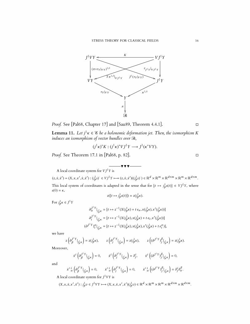
STRESS THEORY FOR CLASSICAL FIELDS 16
B
Y
VY J1Y
J1VY V J1Y
π
τY |VY''
π 1,0
ww
(πτY |VY )1,0
τJ 1Y |V J 1Y
Koo
T π 1,0 |V J 1Ytt J 1(τY |VY ) **
Proof. See [Pal68, Chapter 17] and [Sau89, Theorem 4.4.1].
Lemma 11. Let j1κ ∈ E be a holonomic deformation jet. Then, the isomorphism Kinduces an isomorphism of vector bundles over B,
(j1κ)∗K : (j1κ)∗V J1Y −→ J1(κ∗VY ).Proof. See Theorem 17.1 in [Pal68, p. 82].
HHHA local coordinate system for V J1Y is
(z, x , x ′) = (X ,x ,x ′, x , x ′) : (j1ps)· ∈ V J1Y 7−→ (z, x , x ′)((j1ps)·) ∈ Rd ×Rm ×Rd×m ×Rm ×Rd×m .
This local system of coordinates is adapted in the sense that for [t 7→ j1ps(t)] ∈ V J1Y , wheres(0) = κ,
z([t 7→ j1ps(t)]) = z(j1pκ).For j1pκ ∈ J1Y
∂J 1Yα |j1pκ = [t 7→ z−1(X (j1pκ) + t eα ,x(j1pκ),x ′(j1pκ))]∂J 1Yi |j1pκ = [t 7→ z−1(X (j1pκ),x(j1pκ) + t ei ,x ′(j1pκ))]
(∂ J 1Y )αi |j1pκ = [t 7→ z−1(X (j1pκ),x(j1pκ),x ′(j1pκ) + t eαi )],we have
z(∂J 1Yβ |j1pκ
)= z(j1pκ), z
(∂J 1Yj |j1pκ
)= z(j1pκ), z
((∂ J 1Y )βj |j1pκ
)= z(j1pκ).
Moreover,
x i(∂J 1Yβ |j1pκ
)= 0, x i
(∂J 1Yj |j1pκ
)= δ ij , x i
((∂ J 1Y )βj |j1pκ
)= 0,
andx ′ iα
(∂J 1Yβ |j1pκ
)= 0, x ′ iα
(∂J 1Yj |j1pκ
)= 0, x ′ iα
((∂ J 1Y )βj |j1pκ
)= δ ij δ
βα .
A local coordinate system for J1VY is
(X ,x , x ,x ′, x ′) : j1pv ∈ J1VY 7−→ (X ,x , x ,x ′, x ′)(j1pv) ∈ Rd ×Rm ×Rm ×Rd×m ×Rd×m .
STRESS THEORY FOR CLASSICAL FIELDS 17
For a local section v = vi κ∗∂Yi of κ∗VY ,
Xα (j1pv) = Xα (vp ) x i (j1pv) = x i (vp ) x i (j1pv) = vi (p)
x ′iα (j1pv) = x ′iα (j1pκ) and (x ′)iα (j1pv) = (∂Bα vi )(p).The isomorphism V J1Y ' J1VY is represented by:
K(vi (p) ∂ J 1Yi |j1pκ + (∂
Bα v
i )(p) (∂ J 1Y )αi |j1pκ)= j1p (vi κ∗∂Yi ),
In other words, The local representative K of K is given by
K(X ,x ,x ′, x , x ′) = (X ,x , x ,x ′, x ′).Note that
dπ1,0 ∂ J1Y
α = (π1,0)∗∂Yα dπ1,0 ∂ J1Y
i = (π1,0)∗∂Yi and dπ1,0 (∂ J 1Y )αi = 0. (4.2)
We denote by dxαJ 1Y
, dx iJ 1Y
and (dx J 1Y )iα the corresponding co-frames:
dxαJ 1Y = (π1,0)]dxαY = (π1)]dxαB
and dx iJ 1Y = (π1,0)]dx iY . (4.3)
NNN
4.3. Compatibility and jet prolongation of velocity fields. Evidently, spe-cial attention should be given to configuration jets induced as jets of configu-rations. The analogous situation applies to generalized velocity fields. In thissection, we consider compatible configuration jets and compatible velocity jets.
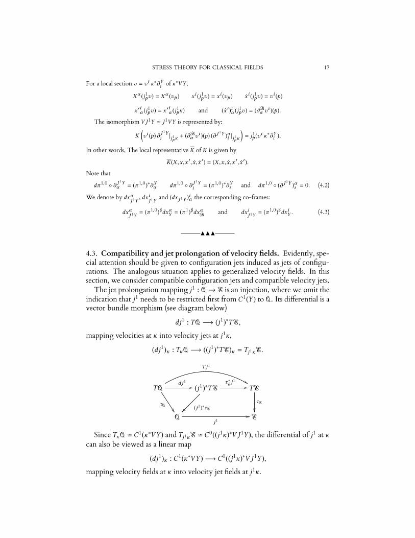
The jet prolongation mapping j1 : Q→ E is an injection, where we omit theindication that j1 needs to be restricted first from C1(Y ) to Q. Its dierential is avector bundle morphism (see diagram below)
dj1 : TQ −→ (j1)∗T E,
mapping velocities at κ into velocity jets at j1κ,
(dj1)κ : TκQ −→ ((j1)∗T E)κ = Tj1κE.
Q E
T ETQ (j1)∗T E
j1//
τQ (j1)∗τE
τE
T j1
&&d j1 //τ ∗Ej1
//
Since TκQ ' C1(κ∗VY ) and Tj1κE' C0((j1κ)∗V J1Y ), the dierential of j1 at κcan also be viewed as a linear map
(dj1)κ : C1(κ∗VY ) −→ C0((j1κ)∗V J1Y ),mapping velocity fields at κ into velocity jet fields at j1κ.

STRESS THEORY FOR CLASSICAL FIELDS 18
Proposition 12. The dierential of j1 can be factored into the action of j1 and a vectorbundle morphism: for v ∈ TκQ ' C1(κ∗VY ),
(dj1)κ (v) = (j1κ)∗K−1 j1v .In other words, (dj1)κ is represented by
j1 : C1(κ∗VY )→ C0(J1(κ∗VY )) ' C0((j1κ)∗V J1Y ),where the last isomorphism follows from Lemma 11.
Proof. For v ∈ TκQ, let s : I → Q be a path of configurations satisfying
s(0) = κ and s(0) = v .By the definition of the dierential via its action on curves,
(dj1)κ (v) = [t 7→ j1s(t)] ∈ Tj1κE.We now view v as a section C1(κ∗VY ), i.e., as a map
p 7→ [t 7→ sp (t)].Then,
j1v = j1[t 7→ s(t)] ∈ C0(J1(κ∗VY )),and
(j1κ)∗K−1 j1v = [t 7→ j1s(t)] ∈ C0((j1κ)∗V J1Y ).
Since (dj1)κ (v) can be identified with j1v, we will use the shorter notation j1vrather than (dj1)κ (v) to denote the corresponding element of Tj1κE, and treat
j1 : C1(κ∗VY ) −→ C0(J1(κ∗VY ))as a representative of (dj1)κ .
HHHUsing local coordinate frames, a velocity field v at κ may be represented locally in the form,
v = vi κ∗∂Yi ,
where vi are dierentiable functions defined on the domain of a chart. Its jet prolongation is thevelocity jet field at j1κ, represented locally as
j1v = vi (j1κ)∗∂ J 1Yi + (∂Bα vi ) (j1κ)∗(∂ J1Y )αi . (4.4)
NNN
5. STRESSES
This section introduces the stress object as a tensor valued measure that rep-resents a force functional, non-uniquely. Particular attention is given to stressesmeasures that are continuous relative to volume measures on the manifold B.
STRESS THEORY FOR CLASSICAL FIELDS 19
5.1. Variational stresses.
Definition 13. The bundle (T ∗E,τ ∗E,E) dual to the bundle of velocity jets T E
is termed the bundle of variational stresses. Given a deformation jet ξ ∈ E, anelement σ ∈ T ∗ξ E is referred to as a variational stress at ξ .
For every deformation jet ξ ∈ E, the vector spaceT ∗ξ Eis the dual of the vectorspace of velocity jets at ξ , Tξ E. By the isomorphism (4.1),
T ∗ξ E' (C0(ξ ∗V J1Y ))∗. (5.1)
Let κ ∈ Q be given. The map
j1 : C1(κ∗VY ) −→ C0((j1κ)∗V J1Y )is an embedding. It follows from the Hahn-Banach theorem that its dual,
(j1)∗ : (C0((j1κ)∗V J1Y ))∗ −→ (C1(κ∗VY ))∗is surjective; to every force at κ, f ∈ (C1(κ∗VY ))∗, there corresponds a (non-unique) variational stress at j1κ, σ ∈ (C0((j1κ)∗V J1Y ))∗, such that
f = (j1)∗σ . (5.2)
That is, for every v ∈ TκQ,f (v) = σ (j1v). (5.3)
Equation (5.3) is a generalization of the principle of virtual work in continuummechanics, and Equation (5.2) is the corresponding generalization of the equi-librium equation.
It should be noted that the (generalized) equilibrium equation is merely arepresentation theorem; it is not a law of physics. Note also that the well-known static indeterminacy—the non-uniqueness of the stress representing agiven force—is reflected by the non-injectivity of (j1)∗, which in turn, followsfrom the fact that j1 is not surjective.
Let κ ∈ Q, hence j1κ ∈ E. By the Riesz representation theorem, the space ofcontinuous linear functionals on C0-sections,
T ∗j1κE' (C0((j1κ)∗V J1Y ))∗,coincides with the space of Radon measures valued in the dual vector bundle((j1κ)∗V J1Y )∗. Locally, a variational stress σ ∈ T ∗
j1κE is represented by a collec-
tion of Radon measures
µi , µαi : 1 ≤ i ≤ m, 1 ≤ α ≤ dso that in case v or σ are supported in the domain of a single chart,
σ (j1v) =∫B
vi dµi +
∫B
(∂Bα vi )dµαi . (5.4)
In the general case, σ (j1v) is evaluated using a partition of unity.

STRESS THEORY FOR CLASSICAL FIELDS 20
5.2. Continuous variational stresses. Equation (5.4) shows that variationalstresses may be as singular as measures. In this section, we restrict our attentionto continuous variational stresses, that is, variational stresses for which the mea-sures µi , µαi are absolutely continuous with respect to some smooth volumeform on B.
Definition 14. The bundle of stress densities is
S = Hom(V J1Y , (π 1)∗ΛdT ∗B).It is a vector bundle over J1Y , with projection which we denote by πS : S →J1Y . For ξ ∈ E,
ξ ∗S = Hom(ξ ∗V J1Y ,ΛdT ∗B),is the C0-bundle of variational stress densities along ξ ; it is a vector bundle overB.
Definition 15. A variational stress σ ∈ T ∗ξ E at ξ ∈ E is termed continuous ifthere exists a variational stress density field at ξ ,
s ∈ C0(ξ ∗S) ' C0(Hom(ξ ∗V J1Y ,ΛdT ∗B)),such that for every velocity jet η at ξ , the virtual power that σ expends on η isgiven by
σ (η) =∫B
s η.
Note that on the left-hand side, η is viewed as an element of Tξ E, whereas onthe right-hand side, η is viewed as an element of C0(ξ ∗V J1Y ). (See below thelocal expressions for continuous variational stress densities.)
Let f be a force at κ and suppose that f is represented by a continuousvariational stress at j1κ, σ ∈ T ∗
j1κE with variational stress density field s ∈
C0(Hom(V J1Y , (π 1)∗ΛdT ∗B)). Then, the virtual power expended by f is givenby
f (v) = σ (j1v) =∫B
s (j1v). (5.5)
5.3. Traction stresses. In classical formulations of continuum mechanics in aEuclidean space, the stress object plays two important roles: it determines thetraction fields on sub-bodies via the Cauchy formula, and it acts on velocity jetsto produce power. For continuous stresses on manifolds, two distinct objectsplay these two roles.
The variational stress, as defined above and as its name suggests, producespower when it acts on velocity jets. The object that determines the tractionfields on the boundaries of sub-bodies will be referred to as traction stress (see[Seg02], where it is referred to as the Cauchy stress, and [Seg13], for the caseof a trivial bundle).

STRESS THEORY FOR CLASSICAL FIELDS 21
Definition 16. The bundle of traction stress densities isT := Hom(VY ,π ∗Λd−1T ∗B).
It is a vector bundle over Y , with projection which we denote by πT : T → Y .For κ ∈ Q,
κ∗T = Hom(κ∗VY ,Λd−1T ∗B),is the bundle of traction stresses along κ; it is a vector bundle over B.
Definition 17. A traction stress density field at κ is a continuous section of thebundle of traction stress densities along κ,
τ ∈ C0(κ∗T) = C0(Hom(κ∗VY ,Λd−1T ∗B)).One would like to restrict traction stress density fields to co-dimension 1
submanifolds of B. In particular, to the boundary of B. Consider therefore,an embedded (d − 1)-dimensional, oriented submanifold V ⊂ B. Denote byιV : V→ B the inclusion. We denote by Y |V the restriction of the fiber bundleY to V. Formally,
Y |V := (ιV)∗Y and π |V := (ιV)∗π : Y |V→ V.
Let (E,πE ,Y ) be a vector bundle over Y (below E will represent the vector bun-dles T and VY ). One can restrict E to V by pulling back E over Y |V usingthe map π ∗ιV to obtain the bundle E|V := (π ∗ιV)∗E with the correspondingprojection
πE |V = (π ∗ιV)∗πE : E|V→ Y |V;see the following diagram.
V B
Y |V Y
E|V E
//ιV
π
π |V
πE
π ∗ιV //
πE |V
π ∗Eπ∗ιV //
Equipped with this notation scheme,T|V = (π ∗ιV)∗T= Hom((π ∗ιV)∗VY , (π ∗ιV)∗π ∗(Λd−1T ∗B))= Hom(VY |V, (π ∗Λd−1T ∗B)|V).
(5.6)
The bundle T|V is the bundle of traction stress densities restricted to V, whichnonetheless act on any (d − 1)-tuple of vectors in TB; it is a vector bundle overY |V.

STRESS THEORY FOR CLASSICAL FIELDS 22
The inclusion ιV : V→ B induces a restriction
(dιV)∗ : ι∗VΛd−1T ∗B−→ Λd−1T ∗V
of (d − 1)-forms to vectors tangent to V. It follows that
(π |V)∗(dιV)∗ : (π |V)∗ι∗VΛd−1T ∗B−→ (π |V)∗Λd−1T ∗V
: π ∗Λd−1T ∗B|V −→ (π |V)∗Λd−1T ∗V.
Composition with the latter defines a vector bundle morphism over Y |V,CV : T|V −→ Hom(VY |V, (π |V)∗Λd−1T ∗V).
The mapping CV is a generalization of the traditional Cauchy formula for con-tinuum mechanics in Euclidean space, τ 7→ τ (n), where n is the unit normal tothe oriented submanifold. We will therefore refer to it as the Cauchy mapping.
Let κ ∈ Q. Denote byκV : V→ Y |V
the restriction of κ to V, namely,
π ∗ιV κV = κ ιV.
Note that for every vector bundle E over Y ,
κ∗VE|V = κ∗V(π ∗ιV)∗E = ι∗Vκ∗E = (κ∗E)|V.Let τ be a traction stress field at κ. Then, ι∗
Vτ is a section of (κ ιV)∗T, where
(κ ιV)∗T ' Hom((κ ιV)∗VY ,ι∗VΛd−1T ∗B)' Hom(κ∗VY |V,Λd−1T ∗B|V),
and we write κ∗VY |V, rather than (κ∗VY )|V, as no ambiguity should arise.Moreover, by (5.6),
κ∗VT|V ' Hom(κ∗VVY |V,Λd−1T ∗B|V) ' (κ ιV)∗T.We may therefore apply the pullback of the Cauchy mapping κ∗
VCV on ι∗
Vτ to
obtain a section
t := (κ∗VCV)(ι∗Vτ ) ∈ C0(Hom(κ∗VY |V,Λd−1T ∗V)).In particular, for the case V= ∂B, a traction stress density field τ at κ inducesvia the Cauchymapping a surface force density field at κ, that is, a vector bundlemorphism
t = (κ∗∂BC∂B)(ι∗∂Bτ ) ∈ C0(Hom(κ∗VY |∂B,Λd−1T ∗∂B)).In order to simplify the notation, we define the morphism
C∂B,κ : C0(Hom(κ∗VY ,Λd−1T ∗B)) −→ C0(Hom(κ∗VY |∂B,Λd−1T ∗∂B))by
τ 7−→ (κ∗∂BC∂B)(ι∗∂Bτ )so that
t = C∂B,κ (τ ).

STRESS THEORY FOR CLASSICAL FIELDS 23
Thus, C∂B,κ is the Cauchy mapping along κ. These formal definitions simplyimply that
t v |∂B = C∂B,κ (τ ) v |∂B = ι]∂B(τ |∂B v |∂B). (5.7)
5.4. The traction stress induced by a variational stress density. The vari-ational stress determines uniquely the traction stress, but the converse does nothold. This section introduces the construction of the traction stress from thevariational stress for the fiber bundle setting.
The vector bundle Vπ 1,0 is a sub-bundle of V J1Y . Its elements are repre-sented by paths in J1Y that are vertical over Y along the fibers of π 1,0. The fiberbundle (J1Y ,π 1,0,Y ) is an ane bundle modeled on the vector bundle [Sau89,Theorem 4.1.11]
π ∗T ∗B⊗Y VY .
Consequently,
Vπ 1,0 ' (π 1)∗T ∗B⊗J 1Y (π 1,0)∗VY ' Hom((π 1)∗TB, (π 1,0)∗VY ).The inclusion I : Vπ 1,0 → V J1Y induces a restriction
I∗ : S −→ Hom(Vπ 1,0, (π 1)∗ΛdT ∗B),defined by
s 7−→ s I.In view of the isomorphism
Hom(Vπ 1,0, (π 1)∗ΛdT ∗B) ' (π 1,0)∗ (π ∗TB⊗Y (VY )∗ ⊗Y π ∗ΛdT ∗B),
we define
C : Hom(Vπ 1,0, (π 1)∗ΛdT ∗B) −→ (π 1,0)∗ ((VY )∗ ⊗Y π ∗Λd−1T ∗B)' (π 1,0)∗T
to be the contraction of the third and first factors in the product, namely,
C(v ⊗ φ ⊗ θ ) = φ ⊗ (v y θ ).Note that C is a vector bundle morphism over J1Y .
Next, defineP : S −→ (π 1,0)∗T,
a vector bundle morphism over J1Y , by
P = C I∗. (5.8)
For κ ∈ Q,Pκ := (j1κ)∗P : (j1κ)∗S −→ κ∗T
maps variational stress densities at j1κ to traction stress densities at κ. It fol-lows that composition with Pκ maps variational stress density fields along j1κ totraction stress fields along κ.
HHHAn element of (j1κ)∗S at p is of the form
sp =(aidx
iJ 1Y |j1pκ + a
αi (dx J 1Y )iα |j1pκ
)⊗ dXp .
STRESS THEORY FOR CLASSICAL FIELDS 24
Its restriction to (Vπ1,0)j1pκ , it can be written as
aαi ∂Bα |p ⊗ dx iY |κp ⊗ dXp .
Then,Pκ (sp ) = aαi dx iY |κp ⊗ (∂Bα ydX )p
Thus, for a variational stress density at j1κ given locally by
s =(si (j1κ)∗dx iJ 1Y + sαi (j1κ)∗(dx J 1Y )iα
)⊗ dX ,
we havePκ s = sαi κ
∗dx iY ⊗ (∂Bα ydX ).
NNN
5.5. The exterior jet of a dierentiable traction stress density. Recall thedefinition of a linear dierential operator (see [Pal68, Chapter 3]).
Definition 18. Let (E,πE ,M) and (F ,πF ,M) be vector bundles over the samebase manifold M . A linear map D : Ck (E) → Ck−1(F ) is called a first-orderlinear dierential operator from E to F if there exists a vector bundle morphismD ∈ L(J1E,F ), such that
D(s) = D j1s, ∀s ∈ Ck (E).Note that J1E is a vector bundle over M only if E is a vector bundle. We willrefer to D as the morphism associated with D.
For convenience, we recall the definitions of the following vector bundles:
body force densities B = Hom(VY ,π ∗ΛdT ∗B),surface force densities T = Hom(VY |∂B, (π |∂B)∗Λd−1T ∗∂B),variational stress densities S = Hom(V J1Y , (π 1)∗ΛdT ∗B),traction stress densities T = Hom(VY ,π ∗Λd−1T ∗B).
Each of these bundles can be pulled back with either κ or j1κ; sections of thepullback bundles are referred to as fields along κ.
Definition 19. Let κ ∈ Q. The exterior jet dierential operator along κ
dκ : C1(κ∗T) −→ C0((j1κ)∗S),is defined as follows. Let τ ∈ C1(κ∗T) be a traction stress density field along κ.Then, for all v ∈ C1(κ∗VY ),
(dκτ ) j1v = d(τ v).Proposition 20. dκ is a well-defined first-order linear dierential operator.

STRESS THEORY FOR CLASSICAL FIELDS 25
Proof. In local coordinates, a traction stress density field along κ takes the form
τ = τ αi κ∗dx iY ⊗ (∂Bα ydX ),
wheredX = dx1B ∧ · · · ∧ dx
dB.
A velocity at κ is given locally by
v = vi κ∗∂Yi ,
hence,τ v = τ αi v
i (∂Bα ydX ).Taking the exterior derivative
d(τ v) = ((∂Bα τ αi )vi + τ αi (∂Bα vi ))dX .
By the local expression (4.4) for j1v, it follows that
dκτ =((∂Bα τ αi ) (j1κ)∗dx iJ 1Y + τ αi (j1κ)∗(dx J 1Y )iα
)⊗ dX
satisfies the defining property of dκτ and depends linearly on τ and its deriva-tives.
5.6. The divergence of dierentiable variational stress densities and theequilibrium field equations. In this section we define the divergence dier-ential operator for dierentiable variational stress densities. The divergenceoperator enables one to tranform the weak form of the compatibility condi-tion between continuous forces and stresses to a strong form of the equilibriumdierential equation. For the rest of this section, we restrict ourselves to C2-configurations and C1-stress density fields.
Proposition 21. Let κ be a C2-configuration. There exists a first-order linear dif-ferential operator mapping dierentiable variational stress density fields along j1κ intocontinuous body force density fields along κ ,
divκ : C1((j1κ)∗S) −→ C0(κ∗B),satisfying for every variational stress density field s ∈ C1((j1κ)∗S) and virtual velocityv ∈ C1(κ∗VY ),
(divκ s) v = dκ (Pκ s) j1v − s j1v . (5.9)
Proof. Using coordinates, a variational stress density field has a local represen-tation in the form
s =(si (j1κ)∗dx iJ 1Y + sαi (j1κ)∗(dx J 1Y )iα
)⊗ dX ,
and a velocity has a local representation
v = vi κ∗∂Yi .
By (4.4),s j1v =
(sivi + sαi (∂Bα vi )
)dX .

STRESS THEORY FOR CLASSICAL FIELDS 26
On the other hand,Pκ s = sαi κ∗dx iY ⊗ (∂Bα ydX ),
anddκ (Pκ s) j1v =
((∂Bα sαi )vi + sαi (∂Bα vi ))dX .
Subtracting, we obtain that
(divκ s) v =((∂Bα sαi )vi − sivi ) dX .
That is,divκ s =
((∂Bα sαi ) − si ) κ∗dx iY ⊗ dX . (5.10)
Consider now a continuous force f ∈ T ∗κQ, given by
f (v) =∫B
b v +∫∂B
t v |∂B,where b ∈ C0(κ∗B) and t ∈ C0(κ∗
∂BT ). Consider further a continuous stress
σ represented by a variational stress density field s ∈ C1((j1κ)∗S). Then, (5.5)takes the form
f (v) = σ (j1v)=
∫B
s (j1v)
= −
∫B
(divκ s) v +∫B
(dκ (Pκ s)) (j1v)
= −
∫B
(divκ s) v +∫B
d((Pκ s) v)
= −
∫B
(divκ s) v +∫∂B
(Pκ s) v .We conclude that f is represented by a variational stress density field s if for
every v ∈ C1(κ∗VY )∫B
b v +∫∂B
t v |∂B = −∫B
(divκ s) v +∫∂B
(Pκ s) v .It is observed that while the restriction of the various terms in the integrand(Pκ s) v to ∂B and to vectors tangent to ∂B is implied in integration theory,formally, in view of (5.7) we write the integrand as C∂B,κ (Pκ s) v. Thus,since equality holds for every v, we obtain
divκ s + b = 0 on B and t = C∂B,κ (Pκ s) on ∂B. (5.11)
In coordinates, equation (5.11) transforms to an underdetermined set of d equa-tions for the (dm +m) components of s.
Note that the above proposition holds if the vector bundle κ∗VY → B isreplaced by an arbitrary vector bundle ρ : W → B, in which case div :L(J1ρ,ΛdT ∗B) −→ L(W ,ΛdT ∗B), which is compatible with [Seg02].

STRESS THEORY FOR CLASSICAL FIELDS 27
6. THE CONTINUUM MECHANICS PROBLEM
It is well known that a given force distribution, does not determine a uniquestress distribution. The source of this non-uniqueness may be traced back toSection 5.1. A unique stress field is determined when additional information inthe form of a constitutive relation is provided. This couples the statics problemdescribed above with the kinematics. The basic notions corresponding to theintroduction of constitutive relations are discussed in this section.
Generally, the continuum mechanics problem takes the following form: thesystem under consideration is subject to external forces, usually dictated by aloading, which is an assignment of a force to every admissible configuration. Aloading may consist of a body force component and a surface force component,and it may be singular or continuous. In analogy, a constitutive relation assignsstresses, regular or singular, to deformation jets, in particular, to jets of con-figurations. The continuum mechanics problem seeks a configuration κ suchthat the stress associated through the constitutive relation with j1κ representsthe force assigned by the loading to κ.
6.1. Loadings.
Definition 22. A loading, F , is a one-form on the configuration space assigninga force Fκ ∈ T ∗κQ to every configuration κ ∈ Q.
Definition 6 of continuous forces extends to a definition of continuous load-ings:
Definition 23. A loading F is termed continuous if there exists a body loadingdensity
B ∈ C0(πB),and a surface loading density
T ∈ C0(πT ),such that for every κ ∈ Q and v ∈ TκQ ' C1(κ∗VY ),
Fκ (v) =∫B
κ∗B v +∫∂B
κ∗∂BT v |∂B,
That is, Fκ is continuous with body force density field κ∗B ∈ C0(κ∗B) and sur-face force density field κ∗
∂BT ∈ C0(κ∗
∂BT ).
Note that by our conventions, we write C0(πB) rather than C0(B), because Bhas multiple bundle structures, and the domain of those sections is not the basemanifold, B.
HHHA body loading density has local representation,
B = Bi dxiY ⊗Y π∗dX
where Bi are real valued continuous functions defined locally on Y .

STRESS THEORY FOR CLASSICAL FIELDS 28
Assume that the chart X is adapted to ∂B so that (X 1, . . . ,Xd−1) is a chart on ∂B and ∂Bd istransversal to T ∂B. Then, one has a volume element ∂Bd ydX on ∂B, and locally,
T = Ti dxiY ⊗Y |∂B π |∗∂B(∂Bd ydX )
where Ti are continuous functions defined locally on Y |∂B. Letv = vi κ∗∂Yi
be a local representation of a velocity at κ. As
κ∗B = (κ∗Bi )κ∗dx iY ⊗B dX and κ∗∂BT = κ∗∂BTi κ
∗∂Bdx
iY ⊗∂B (∂Bd y dX ).
we have the local expression,
(κ∗B) v = vi (κ∗Bi )dX , κ∗∂BT (v∂B) = vi κ∗∂BTi (∂Bd y dX ).If the support of v may be covered by a single chart, we may write Fκ explicitly,
Fκ (v) =∫Bvi (κ∗Bi )dX +
∫∂B
vi (κ∗∂BTi )(∂Bd ydX ).
NNN
Definition 24. A loading F is termed conservative if
F = −dW ,
for some loading potential,W ∈ C1(Q).
Definition 25. A conservative loading is continuous if there exists a body loadingpotential density, which is a C1-section
wB : Y → π ∗ΛdT ∗B, (6.1)
and a boundary loading potential density, which is a C1-section
w∂B : Y |∂B→ (π |∂B)∗Λd−1T ∗∂B, (6.2)
such that the loading potential is given by
W (κ) =∫B
κ∗wB +
∫∂B
κ∗∂Bw∂B
(see diagrams).
B Y
ΛdT ∗B π ∗ΛdT ∗B
κ
77πoo
(τ ∗B)∗κ//
τ ∗B
π ∗τ ∗B
wB
YY
κ∗wB
EE
∂B ι∗∂B
Y
Λd−1T ∗∂B (ι∗∂Bπ )∗Λd−1T ∗∂B
κ∂B
44ι∗∂B
πoo
(τ ∗B)∗κ
//
τ ∗∂B
(ι∗∂B
π )∗τ ∗∂B
w∂B
XX
κ∗∂B
wB
EE

STRESS THEORY FOR CLASSICAL FIELDS 29
Proposition 26. Consider a continuous conservative loading F , the potential functionof which is given by a body loading potential densitywB and boundary loading potentialw∂B. Then, F is a continuous loading with corresponding loading densities
B = −dwB|VY , T = −dw∂B|VY |∂B.Proof. First, we should verify that this relation is well-defined type-wise. By thetypes (6.1) and (6.2) of wB and w∂B, it follows that
dwB ∈ C0(Hom(TY ,w∗BT (π ∗ΛdT ∗B))),
dw∂B ∈ C0(Hom(TY |∂B,w∗∂BT ((π |∂B)∗Λd−1T ∗∂B))).
Restricting to the vertical bundle,
dwB|VY ∈ C0(Hom(VY ,w∗BV (π ∗Λdτ ∗B)))dw∂B|VY |∂B ∈ C0(Hom(VY |∂B,w∗∂BV ((π |∂B)∗Λd−1τ ∗∂B))).
For every vector bundle (E,πE ,Y ), section w : Y → E and a ∈ Y ,
(w∗VπE )a ' (VπE )w (a) ' Ea .
In other words, w∗VπE ' E, and so,
Hom(VY ,w∗BV (π ∗Λdτ ∗B)) ' Hom(VY ,π ∗ΛdT ∗B),Hom(VY |∂B,w∗∂BV ((π |∂B)∗Λd−1τ ∗∂B)) ' Hom(VY |∂B, (π |∂B)∗Λd−1T ∗∂B),
and so, dw |VY and dw∂B|VY |∂B are indeed loading densities.It remains to show that dwB|VY and dw∂B|VY |∂B are the loading densities
corresponding to F = −dW . By definition, for v ∈ TκQ ' C1(κ∗VY ),
dWκ (v) = d
dt
0W γ ,
where γ : I → Q satisfies γ (0) = κ and γ (0) = v. Substituting the representationofW in terms of a density,
dWκ (v) = d
dt
0
[∫B
(γ (t))∗wB +
∫∂B
(γ (t)∂B)∗w∂B
],
=
∫B
d
dt
0(γ (t))∗wB +
∫∂B
d
dt
0(γ (t)∂B)∗w∂B,
where the derivatives ddt
0 (γ (t))∗wB and ddt
0 (γ (t)∂B)∗w∂B are taken pointwisein B and ∂B, respectively.
It follows from the chain rule and the definition of γ thatd
dt
0((γ (t))∗wB)p = (dwB)κp (γ (0))p = (κ∗dwB|VY v)p ,
andd
dt
0((γ (t)∂B)∗w∂B)q = (dw∂B)κq (γ (0))q = ((κ∂B)∗dw∂B|VY |∂B v)q .
STRESS THEORY FOR CLASSICAL FIELDS 30
Thus,
dWκ (v) =∫B
(κ∗dwB|VY ) v +∫∂B
((κ∂B)∗dw∂B|VY |∂B) v,which completes the proof.
HHHIn a local coordinate frame, a loading potential density takes the form,
wB = ωBπ∗dX and w∂B = ω∂Bπ |∗∂B(∂Bd ydX ).where ωB and ω∂B are dierentiable functions defined on the domains of the adapted charts onB and ∂B, respectively. Since the exterior derivatives of the volume elements vanish identically,the loading densities are given locally by
B = −∂iωB dx iY ⊗Y π∗dX , T = −∂iω∂Bdx iY ⊗Y |∂B π |∗∂B(∂Bd ydX ).
NNN
6.2. Constitutive relations. All the notions analyzed above—configurations,velocities, forces, deformation jets and stresses—pertain to a particular theorydepending on the choice of configuration space. Within a particular theory, theproperties of a system are prescribed using a constitutive relation, associating thestate-of-stress with the kinematics.
It is noted that since our base spaceBmay be interpreted naturally as physicalspace-time, constitutive relations may involve time even in cases where it is notexplicitly indicated.
Definition 27. A constitutive relation is a one-form Ψ : E→ T ∗Eon the man-ifold of deformation jets, assigning a stress Ψξ ∈ T ∗ξ E to every deformation jetξ ∈ E.
Since j1 : Q→ E is injective, a constitutive relation Ψ induces a loading
(j1)]Ψ : Q −→ T ∗Q.
By the definition of the pullback of forms, for v ∈ TκQ,
((j1)]Ψ)κ (v) = ((j1)∗Ψ)κ (j1v) = Ψj1κ (j1v),where in the first identity we identified, as before, dj1(v) with j1v.
We note that at this level of generality, and interpretingBas space-time, this,seemingly elastic constitutive relation, is actually non-local, time dependent,and not necessarily causal.
The definition of continuous stresses extends readily to a definition of Ck-dierentiable constitutive relations:
Definition 28. A constitutive relation Ψ : E→ T ∗E is termedCk-dierentiable,k = 0,1, . . . , if there exists a constitutive density, a dierentiable section,
ψ ∈ Ck (πS),

STRESS THEORY FOR CLASSICAL FIELDS 31
such that for every deformation jet ξ ∈ E and for every velocity jet η at ξ ,
Ψξ (η) =∫B
(ξ ∗ψ ) η.In the case of a dierentiable constitutive relation, the induced loading is
given by
((j1)]Ψ)κ (v) = Ψj1κ (j1v) =∫B
((j1κ)∗ψ ) (j1v), v ∈ TκQ.
We note that a dierentiable constitutive relation is local and elastic in the sensethat the stress at a point depends only on the deformation jet at that point.Again, we mention that for the case where B is interpreted as space-time orbody-time, ξ contains components that may reflect velocities. However, his-tory dependence is excluded.
HHHIn coordinates, a constitutive density is represented locally as
ψ =(ψi dx
iJ 1Y +ψ
αi (dx J 1Y )iα
)⊗J 1Y (π1)∗dX ,
where ψi ,ψαi are Ck over the domain of a chart in J1Y .NNN
6.3. The continuum mechanics equations. Given a constitutive relation Ψand a loading F , the continuum mechanics problem seeks a configuration forwhich the stress determined by the constitutive relation represents the loadingfor that configuration. Thus, the condition is expressed by
(j1)]Ψ = F . (6.3)Explicitly, a configuration κ ∈ Q is a solution of (6.3) if for every virtual velocityv at κ,
Ψj1κ (j1v) = Fκ (v).6.4. The dierential form of the continuum mechanics equations. Con-sider the continuummechanics problem in the case of aCk-constitutive densityψ and a continuous loading with densities B and T. A configuration κ ∈ Q
which solves the continuum mechanics problem satisfies∫B
(j1κ)∗ψ j1v =∫B
κ∗B v +∫∂B
κ∗∂BT (v |∂B). (6.4)
for every velocity field v ∈ TκQ ' C1(κ∗VY ).In view of the definition of the divergence, restricting ourselves toC2-configurations
and C1 constitutive densities, we can rewrite these equations as follows:
−
∫B
divκ ((j1κ)∗ψ ) v +∫∂B
((j1κ)∗(P ψ )) v
=
∫B
κ∗B v +∫∂B
κ∗∂BT (v |∂B).

STRESS THEORY FOR CLASSICAL FIELDS 32
Since this hold for every virtual velocityv, we obtain a boundary-value problem
divκ ((j1κ)∗ψ ) + κ∗B = 0, in B,
C∂B,κ ((j1κ)∗(P ψ )) = κ∗∂BT, on ∂B.
HHHLet the loading densities and the constitutive density be given locally by
B = Bi dxiY ⊗Y π∗dX , T = Ti dx
iY ⊗Y |∂B π |∗∂B(∂Bd ydX ),
andψ =
(ψi dx
iJ 1Y +ψ
αi (dx J 1Y )iα
)⊗J 1Y (π1)∗dX ,
Then,
κ∗B = (κ∗Bi )κ∗dx iY ⊗X dX , κ∗∂BT = (κ |∂B)∗Ti (κ |∂B)∗dx iY ⊗∂B (∂Bd ydX )and
(j1κ)∗ψ =(((j1κ)∗ψi ) (j1κ)∗dx iJ 1Y + ((j1κ)∗ψαi ) (j1κ)∗(dx J 1Y )iα
)⊗J 1Y dX .
If follows from the local expressions derived in Sections 5.4 and 5.6 that
(j1κ)∗(P ψ ) = ((j1κ)∗ψαi )κ∗dx iY ⊗ (∂Bα ydX ),and
divκ (j1κψ ) =((j1κ)∗ψi − ∂Bα ((j1κ)∗ψαi )
)κ∗dx iY ⊗ dX ,
so that the field equation is
(j1κ)∗ψi − ∂Bα ((j1κ)∗ψαi ) + (κ∗Bi ) = 0.
Since
ι]∂B
(∂Bα ydX ) =
0, for α , d,∂Bd ydX , for α = d,
(6.5)
the boundary conditions are(j1κ)∗ψdi = (κ |∂B)∗Ti .
NNN
6.5. Conservative constitutive relations.
Definition 29. A constitutive relation is referred to as conservative if there existsan energy function
U ∈ C1(E)such that the constitutive relation is given by
Ψ = dU .
Consider a conservative system with energy functionU , subject to a conser-vative loading F = −dW . Then, the equilibrium equations are
(j1)]Ψ − F = (j1)∗Ψ dj1 − F= (j1)∗dU dj1 + dW= d(U j1 +W ) = 0,

STRESS THEORY FOR CLASSICAL FIELDS 33
where we used the commutativity of external derivatives and pullbacks. Thus,the solution is a critical point of the total energy,
U j1 +W . (6.6)
Definition 30. A conservative constitutive relation is said to be dierentiable ifthere exists a Lagrangian density form, a C2-section
L : J1Y → (π 1)∗ΛdT ∗B,
such that the energy function is of the form
U (ξ ) =∫B
ξ ∗L.
B J1Y
ΛdT ∗B (π 1)∗ΛdT ∗B
ξ//
τ ∗B
//
(π 1)∗τ ∗B
L
hh
ξ ∗L
88
Evidently, dierentiable conservative constitutive relations generalize hyper-elastic constitutive relations to the setting considered in this paper.
Proposition 31. Consider a dierentiable constitutive relation with a Lagrangiandensity L. The resulting constitutive relation is C1 with a constitutive density
ψ = dL|V J 1Y . (6.7)
Equation (6.7) is a generalization of the classical relation between the stress and thederivative of the elastic energy density.
Proof. By definition, for η ∈ Tj1κE' C0((j1κ)∗V J1Y ),
dUj1κ (η) = d
dt
0U (γ (t)),
where γ : I → E satisfies γ (0) = j1κ and γ (0) = η. Substituting the representa-tion of U in terms of a density,
dUj1κ (η) = d
dt
0
∫B
(γ (t))∗L=∫B
d
dt
0(γ (t))∗L,
where the derivative ddt
0 (γ (t))∗L is taken pointwise at every p ∈ B. It followsfrom the chain rule and the definitions of γ and η that
d
dt
0(γ (t))∗L)p = dLj1pκ
(γ (0))p = (dL|V J 1Y )j1pκ ηp ,i.e.,
dUj1κ (η) =∫B
((j1κ)∗dL|V J 1Y ) η,which completes the proof.

STRESS THEORY FOR CLASSICAL FIELDS 34
HHHUsing a coordinate frame, a Lagrangian density is of the form
L= L (π1)∗dX .where L ∈ C∞(J1Y ). Then,
ψ =((∂ J 1Yi L)dx iJ 1Y + ((∂ J
1Y )αi L) (dx J 1Y )iα)⊗J 1Y (π1)∗dX ,
It follows thatψi = ∂
J 1Yi L and ψαi = (∂ J 1Y )αi L.
NNN
7. SOME SPECIAL CASES
We present here a number of examples where the general settings assumeparticularly useful forms.
7.1. Vector bundles. Consider the case where (Y ,π ,B) is a vector bundle. Bythe natural isomorphism TwW 'W for any vector space W, it follows that
(VY )y ' Ty (Yπ (y)) ' Yπ (y), for all y ∈ Y . (7.1)
It follows that for p ∈ B,
(κ∗VY )p ' (VY )κ(p) ' Yπ (κ(p)) = Yp ,
i.e.,
κ∗Vπ ' Y (7.2)independently of κ. As such, this theory may be referred to as linear.
Next, since (Y ,π ,B) is a vector bundle, so is (J1Y ,π 1,B). Thus, in analogy,for any section ξ : B→ J1Y ,
ξ ∗V J1Y ' J1Y . (7.3)
7.2. Ane bundles. Consider the case where (Y ,π ,B) is an ane bundlemodeled on the vector bundle (E,ρ,B) (see [Sau89, p. 48]). It is implied thatfor every y ∈ Y ,
(VY )y ' Ty (Yπ (y)) ' Eπ (y). (7.4)Hence,
κ∗VY ' E (7.5)independently of κ. Likewise, by Lemma 11 ,
(j1κ)∗V J1Y ' J1(κ∗VY ) ' J1E, (7.6)
independently of κ.

STRESS THEORY FOR CLASSICAL FIELDS 35
7.3. The bundle of frames. As mentioned in the introduction, the bundle offrames plays an important role in the geometric theory of continuous distribu-tion of dislocations. Consider the bundle of frames (FB,π ,B) whose fiber atp ∈ B is GL(Rd ,TpB), the space of invertible mappings Rd → TpB viewed asbases (frames) in TpB. Since GL(Rd ,TpB) is an open subset of the vector spaceof linear mappings Hom(Rd ,TpB), FB is a sub-bundle of the vector bundleHom(B×Rd ,TB). We may conclude that for any y ∈ FB,
(VY )y ' Ty (GL(Rd ,Tπ (y)B)) ' Hom(Rd ,Tπ (y)B)and for any frame field κ : B→ FB,
κ∗VY ' Hom(B×Rd ,TB). (7.7)
Again, we may further conclude that
(j1κ)∗V J1Y ' J1(κ∗VY ) ' J1(Hom(Rd ,Tπ (y)B)). (7.8)
7.4. Form-conjugate forces and stresses. Consider the casewhereY = ΛpT ∗B,where 1 ≤ p ≤ d. This is a special case of 7.1 above. It follows that for any κ ∈ Q,κ∗VY ' ΛpT ∗B and (j1κ)∗V J1Y ' J1(ΛpT ∗B). Dierentiable variational stressdensities fields along j1κ are, therefore, sections of Hom(J1(ΛpT ∗B),ΛdT ∗B)and continuous traction stress density fields are sections ofHom(ΛpT ∗B,Λd−1T ∗B).
A particularly simple case follows when the traction stress density field τ =Pκ s is given in terms of a (d − p − 1)-dierential form д by
τ v = д ∧v (7.9)
for any p-dierential form v on B. It follows thatd(τ v) = d(д ∧v),
= dд ∧v + (−1)d−p−1д ∧ dv .Set,
f = dv, J = dд. (7.10)It follows that,
df = 0, dJ = 0. (7.11)The representation of the force∫
B
s j1v =∫B
d((Pκ s) v) −∫B
divκ s v,
=
∫B
d((Pκ s) v) +∫B
b v,
may be written now as∫B
s j1v =∫B
(J ∧v + (−1)d−p−1д ∧ f + b).Assume that d = 4, p = 1 and consider the special case where b = 0. If weinterpret v as the 1-form potential (vector potential) of electrodynamics, the

STRESS THEORY FOR CLASSICAL FIELDS 36
expression we obtained for the power, together with equations (7.10, 7.11) arethe governing equations of electrodynamics. Here, J is interpreted as the 4-current density, f is interpreted as the Faraday 2-form, and д is interpreted asthe Maxwell 2-form. As no metric structure is used, the equations are in theframework of pre-metric electrodynamics (see [HIO06]). In case the Lorentzmetric is used, one can apply the Hodge star operator and write д = ∗f andobtain the usual Maxwell equations in vacuum, as for example in [MTW73,Chapter 3].
In the general case, one obtains a generalization of electrodynamics, referredto as p-form electrodynamics, as in [HT86, HT88]. (For further details see[Seg16].) A dierent theory in which form-conjugate forces appear is the the-ory of dislocations. In the case of dislocations, however, the traction stress doesnot have a simple form as assumed above. In fact, df = 0 implies that no dislo-cations are present (see [ES14, ES15]).
7.5. Trivial fiber bundles. Consider the case where the fiber bundle (Y ,π .B)is trivial, that is
Y = B×M ,
for somem-dimensional manifoldM . A section representing a configuration inthis case is the graph of a mapping B −→ M . Thus, it is natural in the case oftrivial bundles to identify the configuration with such a mapping
κ : B−→ M .
It follows that the configuration space Q is an open subset of the manifold ofmappings C1(B,M).
SinceTY ' TB×TM ,VY = kerTπ may be identified naturally withB×TM .It follows that a generalized velocity at κ may be represented by a mapping
v : B−→ TM , such that, τM v = κ,
or alternatively, with a section of the vector bundle
(κ∗TM ,κ∗τM ,B).The jet bundle J1Y can now be replaced by the jet space of mapping, J1(B,M)
(see [Mic80, Chapter 1]). An element of J1(B,M) is determined by the tangentmapping Tpκ for some mapping κ; Emay be identified with the space of con-tinuous vector bundle morphisms TB→ TM over C1-mappings B→ M .
For further details regarding the forms assumed by continuous forces andstresses, see [Seg13].
7.6. Continuum mechanics on manifolds. The previous example includesthe case of continuum mechanics on manifolds. Here, the manifold M is inter-preted as the physical space S . For continuum mechanics, it is customary to re-quire that configurations satisfy the principle of material impenetrability whichimplies that Q be the space of all embeddings B → S . Indeed, the subset ofembeddings is open in the manifold of mappingsC1(B,S) (see [Hir76, Mic80]).

STRESS THEORY FOR CLASSICAL FIELDS 37
In the classical case, both B and S are 3-dimensional and S is a Euclideanspace.
7.7. Continuawithmicrostructure. Continuummechanics ofmaterials withmicrostructure falls under the case where Y has the structure of a Cartesianproduct B×M , however, the manifold M has the additional structure of a fiberbundle
(M ,ρ,S).The fiber over the point z ∈ S is interpreted as possible micro-states that a mate-rial point located at z may assume. Terms such as “internal variables”, “internaldegrees of freedom”, “order parameters”, etc. are also used for the micro-states.
A configuration of a body with microstructure is a mapping
κ : B−→ M
for whichκ0 := ρ κ : B→ S
is an embedding.For bodies with microstructre, forces and stresses include components that
are conjugate to the micro-velocities and their jets (see [Seg94]).A number of examples of continuawithmicrostructure are discussed in [Mer79,
Cap89]. These include mixtures, liquid crystals, Superfluid helium-3, Cosseratcontinua, etc.
7.8. Group action. We consider the case where for some Lie groupG there isa smooth left action
λ : G × Y −→ Y
such that for all д ∈ G,λд : д × Y −→ Y
is a fiber bundle morphism over the identity of B. Thus, for p ∈ B, the imageof λp : G × p→ Y is contained in Yp .
The tangent mapping
Tλ : TG ×TY −→ TY
may be decomposed into partial tangents, and in particular
T1λ : TG × Y −→ TY
may be restricted to the Lie algebra, TeG, and we obtain
T1λe : TeG × Y −→ TY .
It is observed that the image of T1λe is a subset of the vertical sub-bundle. Itfollows that for any γ ∈ TeG, κ ∈ Q, there is a generalized velocity
vγ : B→ VY , vγ (p) = T1λe (γ ,κ(p)).It would be natural, therefore, to define an equilibrated force as an element
f ∈ T ∗κQ such thatf (vγ ) = 0, for all γ ∈ TeG

STRESS THEORY FOR CLASSICAL FIELDS 38
(see also [Seg94]). Requiring that all forces on all subbodies be equilibratedrestricts the class of stresses. For example, in the classical formulation of con-tinuum mechanics in a Euclidean space, invariance under the Euclidean groupimplies that the components µi of the variational stress vanish and the com-ponents µαi satisfy the usual symmetry conditions for the first Piola-Kirchhostress.
Acknowledgement: RK was partially supported by the Israel Science Foun-dation (Grant No. 661/13), and by a grant from the Ministry of Science, Tech-nology and Space, Israel and the Russian Foundation for Basic Research, theRussian Federation. RS was partially supported by the H. Greenhill Chair forTheoretical and Applied Mechanics and by the Pearlstone Center for Aeronau-tical Engineering Studies at Ben-Gurion University.
REFERENCES[BBS55] B.A. Bilby, R. Bullough, and E. Smith. Continuous distributions of dislocations:
A new application of the methods of non-Riemannian geometry. Proceedings ofthe Royal Society of London, A 231:263–273, 1955.
[Blo79] F. Bloom.Modern Dierential Geometric Techniques in the Theory of Continuous Dis-tributions of Dislocations, volume 733 of Lecture Notes in Mathematics. Springer,1979.
[BSF88] E. Binz, J. Śniatycki, and H. Fischer.Geometry of Classical Fields. North-Holland,1988.
[Cap89] G. Capriz. Continua with Microstructure. Springer, 1989.[dR85] M. de León and P.R. Rodrigues. Generalized Classical Mechanics and Field Theory:
A Geometrical Approach of Lagrangian and Hamiltonian Formalisms Involving HigherOrder Derivatives. North-Holland, 1985.
[EE07] M. Elzanowski and M. Epstein. Material Inhomogeneities and their Evolution.Springer, 2007.
[EEMLRR96] A. Echeverria-Enriquez, M.C. Munoz-Lecanda, and N. Roman-Roy. Geometryof Lagrangian first-order classical field theories. Fortschritte der Physik, 44:235–280, 1996.
[ES14] M. Epstein and R. Segev. Geometric aspects of singular dislocations.Mathematicsand Mechanics of Solids, 19:335–347, 2014. DOI: 10.1177/1081286512465222.
[ES15] M. Epstein and R. Segev. Dierential Geometry and Continuum Mechanics, volume137 of Springer Proceedings in Mathematics and Statistics, chapter 7: On the geom-etry and kinematics of smoothly distributed and singular defects, pages 203–234.Springer, 2015.
[Fra12] T. Frankel. The Geometry of Physics. Cambridge university press, 3 edition, 2012.[GH97] F. Gronwald and F.W. Hehl. Stress and hyperstress as fundamental concepts in
continuummechanics and in relativistic field theory. arXiv:gr-qc/9701054, 1997.[GIMM03] M.J. Gotay, J. Isenberg, J.E. Marsden, and R. Motgomery. Momentum maps and
classical fileds. Part I: Covariant field theory, 2003.[GM75] M. E. Gurtin and L. C. Martins. Cauchy’s theorem in classical physics. Archive for
rational mechanics and analysis, 60:305–324, 1975.[GMS09] G. Giachetta, L. Mangiarotti, and G. Sardansashvily.Advanced Classical Field The-
ory. World Scientific, 2009.[GS77] V. Guillemin and S. Sternberg. Geometric Asymptotics. American Mathematical
Society, 1977.

STRESS THEORY FOR CLASSICAL FIELDS 39
[GW67] M. E. Gurtin andW.Williams. An axiomatic foundation for continuum thermo-dynamics. Archive for Rational Mechanics and Analysis, 26(2):83–117, 1967.
[Heh76] F.W. Hehl. On the energy tensor of spinning massive matter in classical fieldtheory and general relativity. Reports on Mathematical Physics, 9:55–82, 1976.
[Her70] R. Hermann. Vector Bundles in Mathematical Physics. Benjamin, 1970.[HIO06] F.W. Hehl, Y. Itin, and Y.N. Obukhov. Recent developments in premetric elec-
trodynamics. arXiv:physics/0610221v1 [physics.class-ph], October 2006.[Hir76] M. Hirsch. Dierential Topology. Springer, 1976.[HM86] F.W. Hehl and D. McCrea. Bianchi identities and the automatic conservation of
energy-momentum and angular momentum in general-relativistic field theories.Foundations of Physics, 16:267–293, 1986.
[HMMN95] F.W. Hehl, J.D. McCrea, E.W. Mielke, and Y. Ne’eman. Metric-ane gaugetheory of gravity: field equations, Noether identities, world spinors, and breakingof dilation invariance. Physics Reports, 258:1–171, 1995.
[HN91] F.W. Hehl and Y. Ne’eman. Spacetime as a continuum with microstructure andmetric-ane gravity. In P.I. Pronin and et al., editors,Modern Proglems of Theoret-ical Physics: Jubilee Vol of D. Ivanenko’s 85 Birthday., pages 31–52. World Scientific,1991.
[HT86] M. Henneaux and C. Teitelboim. p-form electrodynamics. Foundations of Physics,16(7):593–617, 1986.
[HT88] M. Henneaux and C. Teitelboim. Dynamics of chiral (self-dual) p-forms. PhysicsLetters B, 206:650–654, 1988.
[KM97] A. Kriegl and P.W. Michor. The Convenient Setting of Global Analysis. AmericanMathematical Society, 1997.
[Kom68] J. Komorowski. A modern version of the E. Noether’s theorems in the calculusof variations, i. Studia Mathematica, 29:261–273, 1968.
[Kom69] J. Komorowski. A modern version of the E. Noether’s theorems in the calculusof variations, ii. Studia Mathematica, 32:181–190, 1969.
[Kon55] K. Kondo. Geometry of Elastic Deformation and Incompatibility. Tokyo GakujutsuBenken Fukyu-Kai, IC, 1955.
[Kru71] D. Krupka. Lagrange theory in fiberedmanifolds.Reports onMathematical Physics,2:121–133, 1971.
[KT79] J. Kijowski andW.M. Tuczyjew.A Symplectic Framework for Field Theories. Num-ber 107 in Lecture Notes in Physics. Springer, 1979.
[Lan72] S. Lang. Dierential Manifolds. Addison-Wesley, 1972.[Mer79] N.D. Mermin. The topological theory of defects in ordered media. Reviews of
Modern Physics, 51:591–646, 1979.[Mic80] P.W. Michor. Manifolds of Dierentiable Mappings. Shiva, 1980.[MTW73] C.W. Misner, K.S. Thorne, and J.A. Wheeler. Gravitation. Freeman, 1973.[Nol59] W. Noll. The foundations of classical mechanics in the light of recent advances
in continuum mechanics. In Leon Henkin, Patrick Suppes, and Alfred Tarski,editors, The Axiomatic Method, with Special Reference to Geometry and Physics, pages266–281. North-Holland, 1959. Proceedings of an international symposium heldat the University of California, Berkeley, December 26, 1957-January 4, 1958.
[Nol67] W. Noll. Materially uniform simple bodies with inhomogeneities.Archive for Ra-tional Mechanics and Analysis, 27:1–32, 1967.
[Pal68] R. S. Palais. Foundations of Global Non-Linear Analysis. Benjamin, 1968.[PT01] P. Piccione and D.V. Tausk. On the Banach dierential structure for sets of maps
on non-compact domains. Nonlinear Analysis: Theory, Methods & Applications,46(2):245–265, 2001.
[Ram01] P. Ramond. Field Theory: A Modern Primer. Westview, 2001.

STRESS THEORY FOR CLASSICAL FIELDS 40
[Sau89] D.J. Saunders. The Geometry of J et Bundles, volume 142 of London MathematicalSociety: Lecture Notes Series. Cambridge University Press, 1989.
[Seg81] R. Segev.Dierentiable manifolds and some basic notions of continuum mechanics. PhDthesis, U. of Calgary, 1981.
[Seg86] R. Segev. Forces and the existence of stresses in invariant continuum mechanics.Journal of Mathematical Physics, 27:163–170, 1986.
[Seg94] R. Segev. A geometrical framework for the statics of materials with microstruc-ture. Mathematical Models and Methods in Applied Sciences, 6:871–897, 1994.
[Seg02] R. Segev. Metric-independent analysis of the stress-energy tensor. Journal ofMathematical Physics, 43:3220–3231, 2002.
[Seg13] R. Segev. Notes on metric independent analysis of classical fields. MathematicalMethods in the Applied Sciences, 36:497–566, 2013. DOI: 10.1002/mma.2610.
[Seg16] R. Segev. Continuum mechanics, stresses, currents and electrodynamics. Philo-sophical Transactions of the Royal Society of London A, 374:20150174, 2016. DOI:10.1098/rsta.2015.0174.
[Sil85] M. Silhavy. The existence of the flux vector and the divergence theorem for gen-eral Cauchy fluxes. Archive for Rational Mechanics and Analysis, 90:195–212, 1985.
[Sil91] M. Silhavy. Cauchy’s stress theorem and tensor fields with divergence in Lp .Archive for Rational Mechanics and Analysis, 116:223–255, 1991.
[Sil08] M. Silhavy. Cauchy’s stress theorem for stresses represented by measures. Contin-uum Mechanics and Thermodynamics, 20:75–96, 2008.
[Śniatycki70] J. Śniatycki. On the geometric structure of classical field theory in Lagrangianformulation. Proceedings of the Cambridge Philosophical Society, 68:475–484, 1970.
[TN65] C. A . Truesdell and W. Noll. The nonlinear field theories of mechanics. Springer,1965.
[Tra67] A. Trautman. Noether equations and conservation laws.Communications in Math-ematical Physics, 6:248–261, 1967.
[TT60] C.A. Truesdell and R. Toupin. The Classical Field Theories, volume III/1 ofHand-buch der Physik. Springer, 1960.
[Wan67] C.-C.Wang. On the geometric structures of simple bodies, a mathematical foun-dation for the theory of continuous distributions of dislocations. Archive for Ra-tional Mechanics and Analysis, 27:33–93, 1967.
∗EINSTEIN INSTITUTE OF MATHEMATICS, THE HEBREW UNIVERSITY OF JERUSALEM JERUSALEM,9190401, ISRAEL
∗∗DEPARTMENT OFMECHANICAL ENGINEERING, BEN-GURIONUNIVERSITY OF THENEGEV, BEER-SHEVA 84105, ISRAEL


![COMPLEX CLASSICAL FIELDS: A FRAMEWORK FOR ... … · complex classical fields: a framework for reflection positivity ... eld theory [15, 16]. assuming ... complex classical fields](https://img.dokumen.tips/doc/110x75/5b3c1d957f8b9a560a8d3241/complex-classical-fields-a-framework-for-complex-classical-fields-a-framework.jpg)