Embed Size (px)
Citation preview

Working PaperStress Testing Housing Loan Portfolios: A Regulatory Case StudyAnthony Coleman, Neil Esho, Ilanko Sellathurai, Niruba Thavabalan—issued September 2005
www.apra.gov.au
Australian Prudential Regulation Authority

Australian Prudential Regulation Authority 2
Copyright
The material in this publication is copyright. You may download, display, print or reproduce material in this publication in unaltered form for your personal, non-commercial use or within your organisation, with proper attribution given to the Australian Prudential Regulation Authority (APRA). Other than for any use permitted under the Copyright Act 1968, all other rights are reserved.
Requests for other uses of the information in this publication should be directed to APRA Public Affairs Unit, GPO Box 9836, Sydney NSW 2001 or [email protected]
© Australian Prudential Regulation Authority (2005)
Disclaimer
While APRA endeavours to ensure the quality of this Publication, APRA does not accept any responsibility for the accuracy, completeness or currency of the material included in this Publication, and will not be liable for any loss or damage arising out of any use of, or reliance on, this Publication.
Inquiries
For more information on the contents of this publication contact:
Neil Esho Head of Research Australian Prudential Regulation Authority GPO Box 9836, Sydney NSW 2001
Email: [email protected]
Ackowledgments
Authors: Anthony Coleman, Neil Esho, Ilanko Sellathurai, Niruba Thavabalan.
All authors are from the Australian Prudential Regulation Authority (APRA). We thank Glenn Homan, Charles Littrell, Ian Sharpe, Wilson Sy, participants at the Federal Reserve Bank of San Francisco, Reserve Bank of Australia, and Monetary Authority of Singapore seminar series, and participants at the April 2005 BIS Workshop on Applied Banking Research for helpful comments and suggestions.

Australian Prudential Regulation Authority 3
Against the backdrop of sharply rising house prices and Central Bank warnings that housing credit growth was not sustainable, the Australian Prudential Regulation Authority (APRA) conducted a ‘stress test’ to gauge the resilience of 120 Australian banks, building societies and credit unions to a substantial correction in the housing market. The stress test scenario mapped a 30 per cent fall in house prices to a substantial increase in default and loss rates. The results showed that all 120 institutions would remain solvent under the imposed conditions, however 11 institutions’ capital ratios fell below their regulatory minima. This paper details the stress testing methodology and traces through the various stages of the project, from background research, to stress test design, implementation, supervisory follow-up, public dissemination of the results and resulting policy changes.
Summary

Australian Prudential Regulation Authority 4
Contents
Introduction 6
Developments in the Australian housing market 7
Methodology 9
The base case 9
Probability of default (PD) 10
Loss-given-default (LGD) 12
Mortgage insurance recoveries (MIR) 13
Resource costs (RC) 14
Expected loss 14
Applying shocks to the base case model 15
Probability of default 15
Loss-given-default 16
Mortgage insurance recoveries 16
Additional resource costs 17
Magnitude of the shocks 17
Average PDs and property prices 18
Average LGD and property prices 19
Implementing the stress test 20
The results 21
Sensitivity analysis 24
Summarising the stress test 25
Feedback to entities and public reporting 26
Supervisory implications 27
Follow-up with individual ADIs 27
Extension to lenders mortgage insurance 27
Basel II 27
Conclusions 28

Australian Prudential Regulation Authority 5
Figures 29
Appendix 1—Base case probability of default matrices 36
Appendix 2–Stress case probability of default matrix for all loans 38
Appendix 3–Regressions relating house prices to PD and LGD 39
Appendix 4–Risk profile and stress test results 40
Appendix 5–Project phases and responsibilities 43
Appendix 6—Historical stress events 45
Appendix 7—Regression summary of the stress test model 46
References 47
Australian Prudential Regulation Authority 6
In the five years to June 2003, housing credit in Australia grew by around 120 per cent. The boom in housing lending, driven by historically low interest rates, has been accompanied by a rapid and sustained increase in housing prices (80 per cent increase over the same five year period), and an increasing range of financial products and credit providers, enabling consumers to gain relatively easy access to credit. Similar housing market developments are currently prevailing in Europe, and in pockets of the United States, and have been observed in countries that have recently experienced a boom and bust cycle.
Against this background of a potentially riskier housing loan environment, the Australian Prudential Regulation Authority (APRA) conducted a stress test in 2003. The objectives of the stress test were to: (i) test whether authorised deposit-taking institutions (ADIs)1 could withstand a large increase in mortgage defaults and loss rates without breaching capital adequacy requirements; (ii) examine the processes in place to manage the costs and risks involved in the loan recovery process; and (iii) to identify and direct supervisory action towards those institutions judged to be most at risk should a downturn in the housing market eventuate.
In this paper, we outline how the stress test was undertaken, detail the methodology, present the stress test results and discuss their implications. As such, the paper provides a case study, which other supervisory agencies may utilise in determining their own stress tests. It provides useful background material and working documents to help answer the following questions: How can a housing loan stress test be conducted? What factors may determine the severity of the stress factors applied to probability of default, loss-given-default, and recoveries on mortgage insurance policies? What factors contribute to the successful management of the project? What benefits
Introduction
can be expected from undertaking such a project? What are the limitations of the stress testing methodology and what alternative methods may be adopted?
The stress test was conducted in several phases, beginning with the development of the model, extensive data collection, application of the stress test, and feedback to financial institutions that took part in the stress test, and concluded with public dissemination of the stress test results. This paper details the methodology adopted in each phase of the project.
Unlike credit risk related stress tests typically undertaken by regulatory agencies and financial institutions, which tend to be macro focused2, the stress test outlined in this paper employs a methodology based on micro-level data. In order to use the stress test as a supervisory tool, the effects of the macro shock must be assessed for each entity, and be able to identify the institutions that are most likely to incur a significant increase in defaults and losses. In addition to its micro focus, the stress test captures risks that are typically ignored, such as the risk of denial or adjustment of mortgage insurance claims, and increased costs associated with managing a higher level of loan delinquencies in a stressed environment.
In summary, the main results of the stress test were that Australian ADIs as a group enjoy strong capital positions at present and this strength, though reduced, would not be materially affected under the modelled stress scenario. Over 90 per cent of ADIs would survive the stress event, taken on its own, without breaching minimum regulatory capital requirements. However, the stress testing process highlighted issues with data quality, systems capabilities, and policy procedures at some ADIs, as well as the heavy reliance of some ADIs on lenders mortgage insurers (LMIs) in preventing large losses. Also, it has identified substantial weaknesses in the regulatory framework for LMIs, leading to proposals to reform the LMI capital framework.
1 ADIs include banks, building societies and credit unions. The non-bank deposit-taking institutions are typically mutually-owned, non-profit organisations, which operate under the same regulatory requirements as banks.
2 See for example, Boss (2002).

Australian Prudential Regulation Authority 7
Over the past 20 years there have been significant developments in the Australian housing finance market. Some of the more significant events have included: the removal of price and quantity restrictions on lending in the mid 1980s; the entry of non-deposit-taking mortgage originators (funded by securitisation) in the early 1990s which led to a significant increase in competition and reduction in housing loan interest margins; the rapid growth of broker-originated lending beginning in the late 1990s; and more recently, the growth of higher risk loan products (such as low-documentation and sub-prime loans). In less than twenty years the market has shifted from one that was tightly controlled and characterised by credit rationing, to being highly diverse, competitive, innovative and providing consumers with relatively easy access to credit.3 Since the early 1990s all these developments have been facilitated by a strong economy and more recently by historically low interest rates.
As a consequence of these developments, since 1991 real growth in housing credit has been above 10 per cent annum in all but two years, and above 15 per cent in 2002 and 2003 (see Figure 1). Over the same period, house price growth has also been particularly strong, with real growth generally between 10 and 15 per cent per annum (see Figure 2).
Reflecting the strong growth of housing credit, the lending portfolios of Australian banks have become increasingly reliant on lending secured by residential mortgages. Residential mortgages now account for over 50 per cent of total lending—up from less than 30 per cent in 1990 (see Figure 3). These shifts in portfolio composition have increased the risk exposure of ADIs to a downturn in the housing market.4
Developments in the Australian housing market
Despite the sustained and rapid growth in housing credit and prices, there has been no sign of deterioration in credit quality. The frequency of claims on mortgage insurers by claim year, and the ratio of impaired housing loans to total housing loans reported by Australian banks (for which more recent data is available) are reported in Figure 4. Both series follow a similar path, however the impaired loans ratio is significantly higher than the claim frequency, reflecting the fact that not all defaults lead to losses and claims on mortgage insurers. Based on current estimates, the impaired housing loans ratio for Australian banks is less than 0.2 per cent, with claims on mortgage insurers lower still.
Despite the current low rate of defaults and claims (which are both backward-looking measures of credit risk), a contraction in housing credit and/or house prices represents a significant risk for regulated deposit-taking institutions. This is supported by the historically positive relationship between real housing credit growth and default rates by underwriting year, and between real house price growth and default rates (see Figures 1 and 2).5 There have also been several studies which document a statistically significant relationship between credit growth and problem loans at the individual bank level (see for example Esho and Liaw (2002) and Salas and Saurina (2002)). This suggests that should housing credit and/or house prices revert significantly, mortgage defaults and claims on mortgage insurers would be expected to increase. This would occur as a higher percentage of poor credit risks are accepted during a period of rapid loan growth, resulting in increased credit losses should a shock occur.
3 Some of the characteristics of the Australian residential mortgage lending market that are worth noting include: lending is predominantly on an adjustable rate basis; fixed rate loans generally do not exceed five years and include prepayment penalties; mortgage insurance is provided exclusively by privately owned companies and allows ADIs to claim a 50 per cent capital concession on loans with a loan-to-valuation ratio (LVR) above 80 per cent; interest and other expenses on investment loans are tax deductible, however capital gains are taxed; loans to owner-occupiers do not generate tax deductions or capital gains tax; and in the event of foreclosure, lenders have the right to claim on other (than the secured property) assets of the borrower.
4 Consistent with the recent Australian experience, Schwartz (2001) notes that it is not only an increase in the total supply of bank credit that facilitates rising prices, but shifts in portfolio composition.
5 The zero default rates in 1999 and 2000 reflect the fact that loans originated in these years are unlikely to have defaulted by the year 2000 (the end of the available data series).

Australian Prudential Regulation Authority 8
The risk of a correction in the housing market may be gauged by examining the property market for signs of imbalances. Given the rapid growth in housing credit, it is not surprising that the ratios of household debt to disposable income, and interest payments to disposable income have risen sharply and are at historically high levels (see Figure 5).6 Similarly, property prices, fuelled by low interest rates and easy access to credit, have risen sharply in all capital cities (see Figure 6). In the Sydney market, for example, the ratio of house prices to rental earnings (P/E) has risen to over 35, from being generally in the range of 15 to 20. In order for the P/E ratio to return to 20, Sydney property prices would need to fall by more than 30 per cent, or rents would need to increase significantly (see Figure 7).
In summary, the past 20 years have seen significant changes in the structure and regulation of housing lending in Australia. Reflecting, in part, these changes, and a long and sustained period of economic growth and low interest rates, housing credit and house prices have reached historical highs in recent years. Although there are no current signs that defaults have increased, the sensitivity of Australian deposit-taking institutions to a significant correction in the housing market has increased. It is against this background that APRA developed and conducted a stress test of ADIs in 2003.
6 Figures 5 and 6 are sourced from the Reserve Bank of Australia web site (www.rba.gov.au). See the Financial Stability Review, Reserve Bank of Australia, September 2004, for a more detailed discussion of recent developments in the Australian housing market.

Australian Prudential Regulation Authority 9
Stress testing is an important risk management tool that is used by individual institutions, prudential regulators and central banks to assess the vulnerability of financial institutions, or the financial system more generally, to exceptional but plausible macroeconomic shocks.7 In an extensive review of macroeconomic stress testing methodologies, Sorge (2004) distinguishes between two general approaches to stress testing, the ‘piecewise approach’ and ‘integrated approach’. The piecewise approach generally involves estimating the impact of a macroeconomic shock on a single measure of financial soundness (such as loan write-offs), whereas the integrated approach attempts to model the impact of a macroeconomic shock on multiple risks (such as credit and market risk) and to then determine, at the portfolio level, the impact on the probability distribution of losses. A risk metric, such as Value at Risk (VaR) is then typically used to determine losses at the chosen confidence level.
The approach adopted in this paper is closer in spirit to the piecewise approach than the integrated approach. Like the piecewise approach, the methodology is intuitive and computationally straightforward. However, whereas most piecewise approaches assume linear econometric models, the approach adopted in this study is nonlinear in several aspects, and due to data limitations, less reliant on econometric modelling.
Following the notation in Sorge (2004), the general methodology adopted in this paper can be written as follows:
E(Yi,t+1
/xt+1≥ x) = f {Xt, Zt} (1)
where in the context of this paper, Yi,t+1
denotes the future unknown value of housing loan related credit losses and resource costs for bank i; x
t+1 denotes the
adverse outcomes assumed for the macroeconomic variables (in particular, property prices) from the set of macroeconomic variables Xt; and Zt a set of variables specific to bank i. The strength of the method described below is in the formulation of Zt, which is disaggregated into separate models for the probability of default (PD), loss-given-default (LGD), mortgage insurance recoveries (MIR) and resource costs (RC). The main weakness of the model is in the econometric robustness of the link between the macroeconomic shocks x
t+1 and the bank specific variables which
Methodology
ultimately determine losses in the stress case. This weakness is partly related to data limitations, and also to the fact that Australia has never experienced a nationwide downturn in the housing market of the magnitude that one might describe as a reasonable or plausible stress. Moreover, as noted in the previous section, there have been fundamental structural changes in the industry which limit the comfort provided by historical experience and the usefulness of that historical experience in shaping the design of a stress test.
Moving from the general description of the methodology above to the specific detail, the paper proceeds in three steps. First, the basic mechanics of the model are outlined, which is referred to as the base case (or non-stress case). Second, the paper outlines how shocks are applied to the base case model to produce the stress scenario, and third, the paper discusses how the magnitude of the shocks were determined.
The base case
Expected losses (EL) in the base case are defined as credit-related losses and resource costs associated with managing defaulted loans, less recoveries on mortgage insurance policies. Modifying the standard EL formula, this gives:
ELi = [PD x LGD x EXP
i ] – MIR + RC (2)
where EXPi is the outstanding loan exposure to a
particular risk for bank i; PD is probability of default; LGD is loss-given-default; MIR is mortgage insurance recoveries on insured loans; and RC denotes resource costs. With the exception of exposure, which is specific to the portfolio of bank i, the components of EL are separately modelled as follows:
PD = f (LVR, age, loan type, loan size) (3)
LGD = f (LVR, age) (4)
MIR = f (policy type, age) (5)
RC = f (defaults, average cost of managing a defaulted loan) (6)
There is an extensive literature examining the determinants of defaults and losses on housing loans. However this literature does not model the
7 This follows the International Monetary Fund (IMF) definition of stress testing quoted in Sorge (2004).
i
i
i

Australian Prudential Regulation Authority 10
determinants of mortgage insurance recoveries or the costs associated with managing increased numbers of defaulted loans. The rationale for the formulation of equations 3 to 6, and the method of determining the relationships is outlined below.
Probability of default (PD)
The probability of default is modelled as a function of LVR (at origination)8, age of the loan (since origination), loan size and loan type (investment versus owner- occupied).9
Following the existing literature, the original LVR is expected to be positively related to the probability of default.10 High LVR borrowers are more likely to default as they tend to have a higher proportion of their incomes devoted to debt servicing, typically have lower net worth if owner-occupiers, and have a lower equity buffer to withstand any fall in housing prices.
Although many studies include both the current LVR and LVR at origination, this study does not for several reasons. First, estimating current LVR is problematic as properties are not routinely revalued, and as a result most studies and financial institutions tend to rely on house price indices to derive an estimate of current LVR. Second, while using revaluation indices may work well when there is considerable volatility in house prices, it is less useful when prices are generally increasing over the sample period. This is particularly the case when the model also includes an age or seasoning factor, which will be highly correlated with house price growth and therefore inversely related to the current LVR of a loan. Consistent with the argument that the inclusion of original LVR and loan age as determinants of default circumvents the need for including an estimate of current LVR, Campbell and Dietrich (1983) report a correlation between loan age and current LVR of -0.71.
The relationship between PD and age of a loan is expected to be nonlinear. Default rates are typically low in the year following loan origination, as borrowers facing stressed circumstances are often
able to access other forms of credit or sell assets to maintain repayments for a short period. Similarly, borrowers who have been making loan repayments beyond four years have generally passed the most difficult debt servicing period. These borrowers are likely to have increased their equity position in the property concerned, due to a combination of increasing asset prices and loan repayments, and are therefore less likely to default. Borrowers, two to four years since origination, tend to have the highest default rates under normal market conditions. Campbell and Dietrich (1983) find support for a quadratic relationship between loan age and default. Similarly, the Office of Federal Housing Enterprise Oversight (OFHEO) risk-based capital model and rating agencies models (see Klopfer (2002)) use multiple age categories or dummy variables to account for the nonlinear relationship between loan age and default.
The model includes loan size as a proxy for several risk factors. For a given LVR and loan age, larger loans are likely to have a higher debt servicing burden and are therefore higher risk than smaller loans. Moreover, larger loans are more likely to be secured against properties with a higher luxury component and/or be located in geographical areas that have experienced the greatest price appreciation. In a downturn, properties that have experienced the greatest price appreciation are likely to also experience greater price depreciation, while demand for luxury properties is likely to be impacted more heavily than other properties. Hence, larger loans are expected to be more sensitive to a downturn in housing prices. This intuition is supported by Ambrose, Buttimer and Thibodeau (2001) who find, using a sample of house price data from Dallas County, a U-shaped relationship between house price volatility and the level of house prices. Houses in the highest price decile have the highest volatility, while houses in the middle deciles have the lowest volatility. Relative loan size is also an important risk factor in the OFHEO risk-based capital model, with the default parameters increasing as the relative size of the loan increases.11
8 Unless otherwise stated, references to LVR assume the LVR is calculated at the loan origination date, rather than the current date.9 In determining our base case PDs, we define default as occurring when the borrower is in arrears by 90 or more days worth of payments. 10 See for example Campbell and Dietrich (1983), Calem and LaCour-Little (2004), the Office of Federal Housing Enterprise Oversight (OFHEO, 2003),
rating agencies models quoted in Klopfer (2002), and the Australian case study in Berry, Dalton, Engels and Whiting (1999).11 A counter argument could be that borrowers with large loans have greater wealth (in other forms), and may therefore be better able to cope with a fall
in house prices, and less likely to default.

Australian Prudential Regulation Authority 11
The model distinguishes between two loan types, investment and owner-occupied loans.12 We expect investment loans to have a higher probability of default than owner-occupied loans as borrowers tend to place greater importance on their primary place of residence. Also, investors face the additional risk of rental vacancies, are more likely to finance speculative property investments, and often borrow on an interest-only basis (to maximise tax savings) so that less equity is built up over time.
To obtain the data required to test the relationships between these factors and determine their empirical magnitude, we formulated a survey (Step 3 of the project as outlined in Appendix 5) which was sent to 12 ADIs.13 APRA requested each institution provide its default data over the period January 1998 to December 2002, within various categories of loans.14 One of the key objectives of the data request was to determine the joint probability of default given the
Table 1 Matrix of default probabilities in the base case model
Housing loans with 90 or more days worth of payments in arrears
Average of 12 Australian Banks: 1998–2003
LVR (%) Age (years since origination) P(D/LVR)
<1 1–2 2–3 3–4 4–5 5–6 >6
>100 1.87 3.50 3.92 3.98 3.59 3.33 2.84 3.03
96–100 0.72 1.35 1.51 1.54 1.39 1.29 1.10 1.17
91–95 0.66 1.24 1.39 1.42 1.28 1.18 1.01 1.06
86–90 0.67 1.26 1.41 1.44 1.29 1.20 1.02 1.09
81–85 0.65 1.22 1.37 1.39 1.25 1.16 0.99 1.06
76–80 0.54 1.01 1.13 1.15 1.03 0.96 0.82 0.87
71–75 0.51 0.95 1.07 1.09 0.98 0.91 0.77 0.83
66–70 0.45 0.85 0.95 0.97 0.87 0.81 0.69 0.74
61–65 0.43 0.80 0.90 0.91 0.82 0.76 0.65 0.69
<61 0.40 0.75 0.83 0.85 0.76 0.71 0.60 0.65
P(A) 33 23 15 10 7 5 8
P(A/D) 20 27 19 14 8 5 7
12 Owner-occupied loans are provided to finance dwellings in which the borrower resides, or intends to reside. All other loans are investment loans, and are typically used to finance dwellings that are leased to third parties.
13 The first two steps of the project involved background research and model development. Although the sample of 12 ADIs may seem small, in aggregate several million loan observations were used to calculate the default rates. The 12 ADIs varied considerably by size and geographic diversification.
14 The sample period is characterised by particularly good macroeconomic conditions: annual GDP growth averaged 3.8 per cent (ABS: Chain Volume Measures); the unemployment rate fell and house prices rose rapidly.
15 The methodology ADIs were required to follow in providing the data is available from the authors.
Note: All figures are expressed in percentages.
LVR of the loan at origination and the current age [P(D/(A LVR)]. Assuming original LVR and age are independent and applying Bayes’ Theorem, it can be shown that:
P(D/(A LVR) = (7)
where D denotes default and A the age of the loan since origination. The application of the above relationship considerably simplified the data request. In order to estimate the required joint default probabilities, ADIs had to provide data on the probability of default by LVR category [P(D/LVR)], the age distribution of defaulted loans [P(A/D)], and the age distribution of all loans [P(A)].15
Table 1 shows the probability of default matrix for all loan types and sizes as estimated from Step 3 of the project. The matrix of default probabilities reported in Table 1 is the simple average of the default rates
P(D/LVR) x P (A/D)P(A)

Australian Prudential Regulation Authority 12
reported by the 12 ADIs that participated in the initial phase of the project.16 Default rates were determined for a combination of seven age categories and 10 LVR categories, resulting in a matrix of 70 cells across which default rates vary. Using the same procedure, default matrices were separately estimated for small owner-occupied loans, large owner-occupied loans, small investment loans and large investment loans. This resulted in 280 estimates of the joint probability of default. Appendix 1 reports the four base case matrices, which in practice also varied with portfolio size.17
The matrix of default probabilities reported in Table 1 and in Appendix 1 show that: (i) PD is directly related to LVR; (ii) PDs peak two to four years after origination and decline thereafter; (iii) PDs are higher for larger sized loans than smaller sized loans; and (iv) PDs are higher for investment loans than owner-occupied loans. These results support the general formulation of the PD function given by equation 3, and are consistent with existing empirical evidence.
A limitation of the above analysis is that the model does not include a credit quality (or debt serviceability) measure such as the Fair Isaac and Company (FICO) score commonly used to assess consumer credit in the U.S. The Australian market lacks the equivalent of a FICO score which captures positive credit information. Rather, Australian credit bureaus only record negative credit events. As such Australian lenders have historically relied on rules of thumb, such as the ratio of annual debt obligations to gross income should not exceed 30 per cent. More recently, many lenders and mortgage insurers have moved to model the excess cash flow after meeting debt repayments, taxes and reasonable living expenses. Although this information is collected at origination, it is not always stored in an easily extractable format and is often only recorded as a binary field in a lender’s database (indicating whether the loan application has
met or failed the debt serviceability test). In order to ensure that ADIs could provide the required data without incurring excessive burden, we did not request data on debt serviceability as part of the stress test.
Loss-given-default (LGD)
Losses on defaulted loans arise primarily because of a shortfall between the recoverable value of property and the outstanding debt owed by the borrower. In addition, losses on defaulted loans can increase substantially as a result of legal costs, real estate agent fees, marketing expenses, valuation fees and other expenses involved in the collections process.
In the model, LGD is driven by LVR and the age of the loan. The higher the LVR at origination, the lower the security coverage is likely to be in the event of default, and hence the higher the potential losses. Holding LVR constant, relatively new loans have proportionally higher debt levels, and security against such loans would not have benefited from house price appreciation. Consequently, LGD is expected to decline as the age of a loan increases. The use of LVR and age as primary determinants of LGD is consistent with the net recovery model (1- LGD) estimated by Calem and LaCour-Little (2004).
In order to create a matrix of LGDs (given age and LVR) that followed the same format as the PD matrix, we used historical data supplied by the mortgage insurance industry. These data show that claims on mortgage insurers have a long-run average of approximately 20 per cent.18 The historical relationship between LVR and LGD in the data was counter-intuitive. It showed that, after controlling for loan size, LGD is negatively related to LVR. Conversely, in its May 2001 submission to the Basel Committee on Banking Supervision, GE Capital Mortgage Corporation proposed a set of factors based on ratings agency data which argued that LGD is positively related to LVR.19
16 In the application of the stress test we varied the base case default rates according to the size of the bank’s portfolio. This accounted for the greater diversification available to large, nationally-diversified institutions.
17 The definition of a large loan varied from $200,000 to $500,000 depending on the size of the bank’s lending portfolio. 18 See Australian LMI Industry Historical Experience, Insurance Council of Australia, 2001. 19 GE Capital Mortgage Corporation is the residential mortgage insurance, lending and services affiliate of GE Capital, one of the largest financial services
companies in the world, and the largest mortgage insurer in Australia.

Australian Prudential Regulation Authority 13
Mortgage insurance recoveries (MIR)
In addition to the LGD, the ultimate loss to a lender will depend on both the level of mortgage insurance coverage held by the ADI and mortgage insurance payout ratios. APRA conducted a series of visits to LMIs as part of phase 3 of the project (see Appendix 5).
Two general factors were identified as determinants of mortgage insurance payout ratios: whether the insurance was directly underwritten by the LMI or whether it was written under ‘open policy’, and the age of the loan. Open policy is where the LMI provides the ADI with a LMI policy guideline that allows the ADI to assume cover will be provided if the guidelines have been met. Delegated underwriting is a variant of open policy, and involves the LMI delegating the insurance underwriting to the ADI, subject to the ADI complying with its own lending policies.
Historical claim files reviewed by APRA during a series of on-site visits to three LMIs suggested that payouts are lower for open policy contracts than directly underwritten contracts because the LMI’s
Rather than rely on the historical data for this part of the analysis, we assumed that the average LGD applies to loans with an original LVR of 76 to 80 per cent, and then applied the GE risk factors to produce a positive relationship between LVR and LGD.20 The APRA model utilises these factors to model the relationship between LGD and LVR, assigning a factor of one to the 76 to 80 per cent LVR category, with higher factors for higher LVR loans and lower factors for lower LVR loans. To illustrate, a factor of 1.41 is applied to loans in the 91 to 95 per cent LVR category, which results in an assumed LGD of 28.2 per cent (= 1.41 x 20 per cent).
In the base case, LGD is held constant across age categories. However, in the stressed scenarios discussed below, LGD is assumed to decline with age of the loan. Similar to the PD matrix, an LGD matrix is produced (see Table 2), which houses the LGD parameters for each of the 70 risk categories.21
However, unlike the PD matrices, the LGD matrix does not vary with loan type or loan size.
Table 2 Matrix of LGDs in the base case model
LGDs using a combination of Australian LMI data and rating agency risk factors
LVR (%) Age (years since origination) LVR factor
<1 1–2 2–3 3–4 4–5 5–6 >6
96–100 29.2 29.2 29.2 29.2 29.2 29.2 29.2 1.46
91–95 28.2 28.2 28.2 28.2 28.2 28.2 28.2 1.41
86–90 25.8 25.8 25.8 25.8 25.8 25.8 25.8 1.29
81–85 23.0 23.0 23.0 23.0 23.0 23.0 23.0 1.15
76–80 20.0 20.0 20.0 20.0 20.0 20.0 20.0 1.00
71–75 16.6 16.6 16.6 16.6 16.6 16.6 16.6 0.83
66–70 12.6 12.6 12.6 12.6 12.6 12.6 12.6 0.63
61–65 8.0 8.0 8.0 8.0 8.0 8.0 8.0 0.40
<61 3.0 3.0 3.0 3.0 3.0 3.0 3.0 0.15
LGD and LVR data are expressed in percentages.
20 After we collected the exposure data, we were able to determine that anchoring the 20 per cent LGD to the 76-80 LVR category equated to an average LGD of 15 per cent (assuming the base case default probabilities).
21 With hindsight we believe that setting a minimum LGD of around 10 to 15 per cent would be more appropriate than allowing the LGD to fall to as low as three per cent.

Australian Prudential Regulation Authority 14
terms and conditions are less likely to have been followed precisely. Also, payout ratios are likely to be higher for older loans. If a loan defaults shortly after origination, it is more likely that an error has been made at origination and that LMI policies have not been followed, requiring some adjustment to the claim made by the lender. Conversely, loans that default well after origination are more likely to be the result of changes in the borrower’s circumstances rather than the result of poor loan origination procedures, in which case the LMI is more likely to pay claims in full.
Converting the knowledge gained through file reviews to an empirical model is necessarily subjective. Nevertheless, we felt it was important to account for this risk, given the fact ADIs had ignored it in their own stress testing, that academic studies generally assume 100 per cent recovery on mortgage insured loans (see Calem and LaCour-Little (2004)), and the U.K experience of the early 1990s where claim adjustments and denials were common. To minimise subjectivity, we disaggregated the final payout ratio into smaller components, for which we had collected information as part of the file reviews. Therefore, the overall payout ratio was constructed using the following components:
Payout Ratioi,t
= (1 – DRi,t
– Ai,t
) x 100% + Ai,t
x APRi,t
(8)
for i equal to open policy or direct underwriting; t equal to seasoning factor; and where DR is the rate of complete claim denial; A is the rate of claim adjustment; and APR is the payout ratio on adjusted claims.
By definition, the payout ratio on claims that are not denied or adjusted (1-DR-A) is equal to 100 per cent, the payout ratio on adjusted claims is given by APR, and again by definition, the payout ratio on denied claims is zero. The weighted sum of the payout ratios on paid, adjusted and denied claims gives the overall payout ratio. The base case inputs and payout ratios by policy type and age are presented in Table 3.
Consistent with our current observations of low claims and high payout ratios, the base case payout ratios range from 96 to 99.5 per cent.
Resource costs (RC)
A final consideration of the stress test is the additional resource costs that an ADI will incur as a result of rising defaults. In particular, the focus is on the increased costs of employing staff in the collections department to manage loans in default and any additional outsourcing costs an institution may incur. In the base case additional resource costs are assumed to be zero, as ADIs already have a collections function in place and deal with the current number of defaulted loans.
Expected loss
In order to calculate expected losses, information is required on the current housing loan exposures (EXP) of ADIs, their mortgage insurance coverage and resource costs associated with managing defaulted loans. APRA collected these data from 120 ADIs and
Table 3 Payout ratios on mortgage insured loans in the base case model*
Less than 2 years 2 to 4 years Greater than 4 years
Open policy
Denial ratio 0 0 0
Adjustment ratio 20 10 10
Adjusted PR 80 80 80
Payout ratio 96 98 98
Direct underwriting
Denial ratio 0 0 0
Adjustment ratio 10 5 5
Adjusted PR 90 90 90
Payout ratio 99 99.5 99.5
* All data expressed in percentages.

Australian Prudential Regulation Authority 15
calculated expected losses using equations 2 to 6. The 120 ADIs were chosen on the basis of a minimum on-balance-sheet housing loan portfolio of $20 million. By comparison, the four largest lenders each have housing loan portfolios in excess of $50 billion.
Applying shocks to the base case model
The stress test focuses on the impact of a housing market downturn on the capital position of ADIs, and less on the potential causes of that downturn. As such, the model does not explicitly model the future path of interest rates, unemployment, credit growth or other exogenous macroeconomic factors that could affect house prices, default rates and losses. Rather, property prices are taken as a macro factor, and it is assumed that if an interest rate or unemployment shock were to occur, such a shock would feed through to house prices. The study then attempts to calibrate the stress scenario to a 30 per cent fall in property prices.
The impact of a housing price shock in the model is captured by estimating under a stress scenario: the increase in the probability of default (PD); the increase in the loss-given-default (LGD); the decrease in recoveries that can be expected on mortgage-insured loans; and the additional resource costs required to manage the larger volume of defaulted loans. To summarise, the total losses (TL) (expected plus unexpected losses) are given by the equation below, where the ‘s’ superscript denotes a stressed parameter:
TL = PDs x LGDs x EXP – MIRs + RCs (9)
This section explains how key inputs in the model are altered to produce the stress scenarios, while the following section examines how the actual magnitudes of the stress factors were determined.
Probability of default
The model assumes the PD of high LVR loans will be more sensitive to stressful conditions than the PD of low LVR loans. That is, for a given negative shock to house prices (or other adverse macroeconomic event), the PD of high LVR loans will increase by a greater magnitude than the PD of low LVR loans. This is based on the fact that for a given fall in house prices, a much
greater proportion of high LVR loans will be in a position of negative equity and therefore more prone to default. Also, the magnitude of the negative equity position will be an increasing function of the original LVR. The non-parallel shift in the relationship between PD and LVR assumed in the severe stress scenario is illustrated in Figure 8. Note again that the base case default curve is derived from the data provided by the 12 ADIs that participated in an earlier phase of the project.
The ‘kink’ in the stress scenario default curve at the 76 to 80 per cent LVR category requires some explanation. Although the kink is not evident in the base case relationship between LVR and PD, it was observed in data provided by some ADIs. On that basis a higher stress factor was applied to loans in the 76 to 80 per cent LVR category, resulting in the kink in the stress scenario. This approach assumes borrowers and ADIs have an incentive to avoid mortgage insurance (or higher capital requirements) by arbitrarily structuring loans so that the original LVR is less than 80 per cent.22 This implies that the LVR of loans in this LVR band is understated, and therefore that the PDs of some loans in this category are understated.
The model also includes an age effect when applying stress to the base case model. This is achieved by shifting the age distribution of defaults so that, relative to the base case, the distribution of defaulted loans includes a higher percentage of new loans and a smaller percentage of older loans (see Figure 9). This assumption is based on the expectation that new borrowers face a higher repayment burden and therefore are more sensitive to a fall in house prices. Also, new borrowers are more likely to find themselves in a negative equity position, should house prices fall. This shift in the age distribution is supported by an analysis of the age distribution of claims on mortgage insurers during the stress periods experienced by the state of Queensland in the mid 1980s and Victoria in the early 1990s.
Combining the stress factor applied to the PD given LVR curve and the age distribution of defaults produces the stress case default matrix. Figure 10 shows the relationship between default and age in the stress case for loans in the 76 to 80 per cent LVR category. This represents a single row of the
22 Loans with an LVR above 80 per cent are risk-weighted at 100 per cent, unless mortgage-insured, in which case a 50 per cent risk-weight is applied.

Australian Prudential Regulation Authority 16
stressed case default matrix. It is important to note that Figure 10 represents the outcome of the stress applied to the PD given LVR curve and age distribution of defaults. That is, the stressed relationship between default and age is the result of the other inputs being stressed, rather than a direct stress being applied to the relationship between default and age.
Finally, there is minimal difference in relative stress factors applied to loan size or loan type, except for the fact that some loan categories, such as large loans and investment loans, have higher starting default rates than small loans and owner-occupied loans. The industry average stress case default matrix for all loans is reported in Appendix 2.
Loss-given-default
Under stressed conditions and falling property prices, LGD will increase as the price obtainable for security diminishes relative to the outstanding loan amount, which does not change. Higher LVR loans are likely to suffer relatively higher increases in LGD as the lender is already at the margin in terms of being able to recover the full loan amount. Hence the LGD on high LVR loans is more sensitive to a house price shock than low LVR loans. The non-parallel shift in the relationship between LGD and LVR is shown in Figure 11.
New loans are likely to experience relatively higher increases in LGD under stressful conditions than older loans. This is because older loans would have benefited from increasing property prices in the preceding years. This implies that relative to newer loans, the value of the property at the time of default would be significantly higher compared to the outstanding balance and a greater proportion of the loan amount recovered. For loans in the 76 to 80 per cent LVR category, the shift in the relationship between LGD and age from the base case to the stress case is shown in Figure 12. Note that in the 76 to 80 per cent LVR band, the stressed case LGD falls below the base case LGD when loan age is greater than five years. This reflects the expectation that LGD is likely to decline with loan age, which is not captured in the base case.
Mortgage insurance recoveries
Mortgage insurance recoveries are assumed to decline as housing prices fall because of adjustments to claims from ADIs with less experience in satisfying the terms and conditions of the relevant mortgage insurance contracts. Greater effects are assumed for newer loans and those loans written under open policy. The matrix of payout ratios is presented in Table 4.
Table 4 Payout ratios on mortgage insured loans in the stress case *
Less than 2 years 2 to 4 years Greater than 4 years
Open policy
Denial ratio 15 10 5
Adjustment ratio 40 30 30
Adjusted PR 60 60 70
Payout ratio 69 78 86
Direct underwriting
Denial ratio 10 5 5
Adjustment ratio 30 20 10
Adjusted PR 70 70 80
Payout ratio 81 89 93
* All data expressed in percentages.

Australian Prudential Regulation Authority 17
Additional resource costs
The additional resource costs required under stressed conditions are computed by determining the number of additional defaults (under stress) and multiplying by the average annual cost of managing a defaulted loan. This value is added to the expected loss figure for the institution to arrive at the total expected loss.
Additional resource costs arise in the form of the increased numbers of staff that need to be employed, either internally or through outsourcing arrangements. This is as a direct result of the increased number of defaulted loans, which need to be managed, due to the onset of the stressed environment.
The stress test model incorporates an add-on to total losses in the form of additional resource costs. Additional resource costs are assumed to be zero in the base case because ADIs already have a collections function in place and deal with an ‘average’ or ‘current’ number of defaulted loans. The additional resource costs must reflect this and therefore must take into account the current number of defaulted loans managed and the salary costs per collections staff member.
Four items of information were required from ADIs to estimate additional resource costs that would arise in a stressed environment. These were:
(a) average annual number of defaulted loans managed by a single full-time-equivalent (FTE) employee in credit management;
(b) average annual total cost of a single FTE employee managing defaulted loans (salary);
(c) total number of loans currently in default; and
(d) current outsourcing costs.
To quantify the additional resource costs, the stress test model combines these figures with the predicted number of defaults in the stress test scenario according to the formula:
Additional RC = additional defaults* (average cost of internally managing a default + average cost of outsourcing the management of a default)
where:
additional defaults = predicted defaults – current defaults; average cost of internally managing a default = b/a; and average cost of outsourcing the management of a default = d/c.
A scale adjustment was also applied to the estimate of additional resource costs. Larger institutions with established collections and credit management processes are likely to benefit from scale economies when faced with a rising numbers of defaults, and are more likely to be able to divert resources from other areas within the institution. To account for this, the stress test model gave a 25 per cent concession for defaulted loans above 3,000 and less than 10,000 and a 50 per cent cost concession for defaulted loans above 10,000. The cut-offs, though somewhat subjective, were determined with reference to estimates of likely scale economies supplied by the ADIs.
Magnitude of the shocks
A recent study by Helbling and Terrones (2003), examined the impact of bursting housing price bubbles in 14 countries (including Australia) over the 1970 to 2002 period. The study identified 20 housing price crashes, and found on average that a housing price crash occurred once every 20 years, lasted about four years, involved a decline in real prices of 30 per cent, and was associated with an output loss equivalent to 8 per cent of GDP. Also, the study found that 40 per cent of housing price booms ended in busts, and that, relative to equity price crashes, housing price crashes were associated with faster and more severe macroeconomic and financial developments.23
With the historical association between falling property prices, macroeconomic and financial developments in mind, the stress factors applied in the APRA model have been broadly calibrated to historical stress periods in the Australian economy and, in particular, stress periods in housing lending. Over the past 20 years, housing loan default rates by underwriting year have peaks in 1985, 1989 and 1994. The peaks in both the rate of default and LGD precede falls in the real value of residential property and coincide with adverse macroeconomic circumstances. In 1986, interest rates
23 The theoretical justification for these findings relate to the larger wealth effects associated with falling housing prices than equity prices, the greater role of financial intermediaries in funding housing relative to equity investment, and the feedback effects associated with the responses of intermediaries to falling collateral values.

Australian Prudential Regulation Authority 18
on housing lending rose by 200 basis points to 15.5 per cent before peaking in 1989 at 17 per cent; in 1991 Australia experienced a recession; and, in the 1994 calendar year, official interest rates rose by 275 basis points.
We used several methods to determine the relationship between changes in property prices and average default rates and losses given default. Although the data are limited, a statistically significant inverse relationship was found between average default rates (and LGD) on housing loans and real growth in property prices.
Average PDs and property prices
Over the 21 years (1980 to 2000) for which aggregate annual data is available, it was estimated that a 30 per cent fall in real property prices would result in the average default rates (by underwriting year) presented in Table 5. The estimates in Table 5 are derived using the regression coefficients reported in Appendix 3. To illustrate, the estimated effect of a 30 per cent fall in house prices on loans originated in the prior year is equal to 1/(1+ e–(-4.4762 – 0.3*(-5.3135))) = 5.3 per cent. Following the same procedure we then estimate the effect of a 30 per cent fall in prices on loans originated in earlier years, and by LVR categories.
The estimates in Table 5 show that average default rates are likely to vary considerably by loan age and original LVR. For loans originated in the 12 months preceding a fall in house prices, the results show average default rates for all loans increase from a historical average of 1 per cent to 5.3 per cent and from 2 per cent to 11.1 per cent for loans with
Table 5 Estimated default rates by underwriting year*
Loan category Loans originated in the year preceding the fall
in prices
Loans originated two years prior to the fall
in prices
Historical average default rate by
underwriting year
All loans 5.3 2.5 1.0
LVR > 90% 11.1 4.8 2.0
70% < LVR < 80% 4.6 1.8 0.5
* All data expressed in percentages.
an original LVR greater than 90 per cent. Default rates for the highest risk loans (those originated immediately prior to a shock) are, relative to historical average default rates, higher by a factor of five to nine. This compares to the modelled stress case default probabilities which are on average roughly five times the magnitude of the base case default rates, with a range from 1.5 (at the 5th percentile) to 13 (at the 95th percentile).
The estimates in Table 5 are based on a small sample and do not control for other macroeconomic determinants of default, such as unemployment and interest rates. However, to the extent that changes in real property prices are correlated with other macroeconomic variables, the estimated effect of the fall in housing prices on average default rates will also reflect the effects due to other macroeconomic factors.24
In Figure 13, the model default rates (by LVR category) are compared with historical experience. Consistent with the assumption of the model, high LVR loans are more sensitive to default under stressful conditions than lower LVR loans. The default curve in the model is more severe than the worst case default rates (claim rates) experienced by Australian LMIs, for any given LVR category, over the period 1980 to 2000. The LMI data, which is presented on both a policy year and claim year basis, shows that the worst case national claim experience of Australian LMIs, within any given LVR band, is significantly lower than the modelled stress scenario. Also, the policy year claim frequency is 8 to 18 times the magnitude of the claim year claim frequency.
24 This assumes that the regression model estimated in Appendix 3 is a valid reduced form. That is, house prices are exogenous, while unemployment and interest rates are endogenous.
Australian Prudential Regulation Authority 19
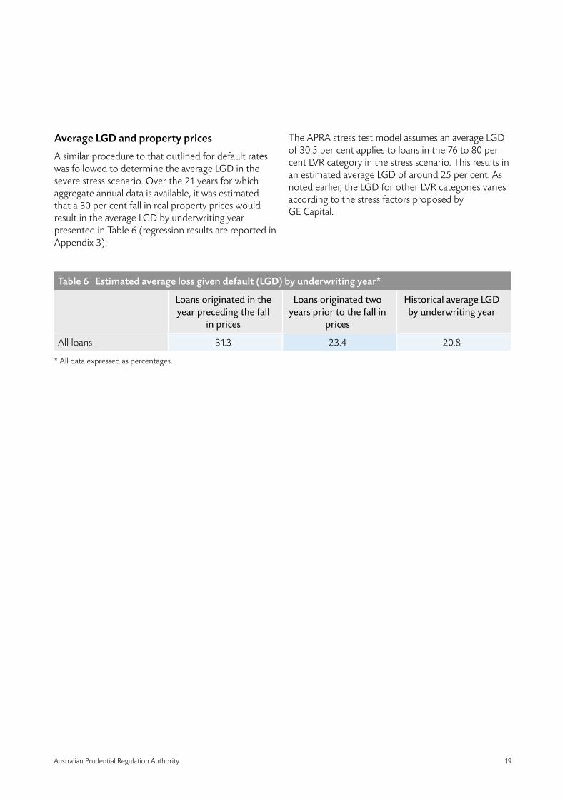
Average LGD and property prices
A similar procedure to that outlined for default rates was followed to determine the average LGD in the severe stress scenario. Over the 21 years for which aggregate annual data is available, it was estimated that a 30 per cent fall in real property prices would result in the average LGD by underwriting year presented in Table 6 (regression results are reported in Appendix 3):
Table 6 Estimated average loss given default (LGD) by underwriting year*
Loans originated in the year preceding the fall
in prices
Loans originated two years prior to the fall in
prices
Historical average LGD by underwriting year
All loans 31.3 23.4 20.8
The APRA stress test model assumes an average LGD of 30.5 per cent applies to loans in the 76 to 80 per cent LVR category in the stress scenario. This results in an estimated average LGD of around 25 per cent. As noted earlier, the LGD for other LVR categories varies according to the stress factors proposed by GE Capital.
* All data expressed as percentages.
Australian Prudential Regulation Authority 20
The key phases of the project and the responsibilities of the major groups are outlined in Appendix 5. The design of the stress test and the central coordination of the project was undertaken by a core team of up to four research staff, with one staff member dedicated to the project on a full-time basis and others used on a need basis. The project was completed in 12 months, and involved a wide cross section of staff from within APRA and a wide cross section of the ADI and LMI industry. As with most projects, the success of the project was facilitated by strong support from senior management, and by the role played by the front-line supervisors. Given the small research team, it would have been difficult to collect the data, perform the necessary data checks and follow-up supervisory action without the contribution of the supervisory staff whose full-time job is to monitor the individual ADIs. To facilitate the involvement of front-line supervisors, much effort was put into explaining the rationale and mechanics of the stress test model, and in making the operational aspects of the stress test user-friendly.
Implementing the stress test

Australian Prudential Regulation Authority 21
A summary of the aggregate on-balance-sheet housing loan portfolios of Australian ADIs in early 2003 by loan age and LVR is provided in Table 7. It shows that approximately 20 per cent of loans had an LVR greater than 80 per cent, with only 2 per cent of loans with an LVR at origination above 95 per cent. A striking feature of the data is the stability of the median LVR, which for all age categories is in the range of 71–75 per cent. While this is suggestive of very little change in the median LVR over time, it does not tell us whether all loans that originated in prior years necessarily had a median LVR of 71–75 per cent, as this would depend on the LVR of matured and refinanced loans. Reflecting the very rapid growth in credit, 77 per cent of loans were originated within the last three years of the sample period.
Disaggregating the LVR distribution by various loan categories, shows that investment loans account for a third of total loans, that 18 per cent of loans are
The results
Table 7 Distribution of housing loans by LVR and loan age
LVR
Age of the loan (years since origination)
<1 1–2 2–3 3–4 4–5 5–6 >6 Total
<61 13 7 4 3 2 1 2 31
61–65 2 1 1 0 0 0 0 5
66–70 5 2 1 1 1 0 0 10
71–75 5 3 1 1 2 1 1 13
76–80 9 5 3 2 1 1 1 21
81–85 2 1 0 0 0 0 0 4
85–90 3 2 1 1 0 0 0 8
90–95 3 2 1 1 0 0 0 6
96–100 0 0 0 0 0 0 0 1
>100 0 0 0 0 0 0 0 1
Total 42 23 12 9 6 3 5 100
Median LVR 71–75 71–75 71–75 71–75 71–75 71–75 71–75 71–75
mortgage-insured, and that 17 per cent of loans have an initial loan amount of $500,000 or greater (see Table 8). As expected the distribution of mortgage-insured loans is skewed to high LVR loans, with a median LVR of 85 to 90 per cent. Conversely, the median investment loan has an LVR of 66 to 70 per cent, which implies that lenders offset the higher inherent risk of investment lending by reducing LVR. It is unlikely that investment loan borrowers self select lower LVR loans than owner-occupiers, given that investors have a tax incentive to increase leverage.
The age distribution of loans by different loan types is reported in Table 9. There is very little variation in the seasoning of loans across the owner-occupied, investment and mortgage insured categories. In the large category, there is evidence of substantial growth in the last year of the sample period, with over 50 per cent of large loans originated in that period. This also reflects rising house prices.
Data as at March 2003. With the exception of LVR, all data is expressed as a percentage of total housing loans. LVR is in per cent.

Australian Prudential Regulation Authority 22
Table 8 The LVR distribution of housing loans by loan type
LVR Owner-occupied Investment loan Mortgage insured Large loans*
<61 28 38 10 27
61–65 5 6 2 6
66–70 11 8 2 15
71–75 14 11 2 19
76–80 19 23 6 18
81–85 4 3 10 4
85–90 9 7 32 6
90–95 8 3 31 2
96–100 1 1 3 1
>100 1 1 1 3
Median LVR 71–75 66–70 85–90 71–75
% of all loans 66 34 18 17
Table 9 The age distribution of housing loans by loan type
Age (years) Owner-occupied Investment loan Mortgage insured Large loans*
<1 41 43 40 53
1–2 23 22 25 24
2–3 12 12 12 10
3–4 9 9 8 6
4–5 6 6 5 4
5–6 3 3 3 2
> 6 3 4 7 2
* Data as at March 2003. The large loan category only applies to loans greater than $500,000. Data is expressed in percentage terms, and sums to 100 per cent within each loan category.
* The large loan category only applies to loans greater than $500,000. Data is expressed in percentage terms, and sums to 100 per cent within each loan category.

Australian Prudential Regulation Authority 23
The upper panel of Table 10 provides further detail on the risk profile of the housing portfolios of Australian ADIs. One of the surprising aspects of the data was the finding that 34 per cent of loans above 80 per cent LVR were reported as being uninsured. To some extent this reflected deviations from stated lending policies, but was also influenced by data quality issues. There is considerable variation in the risk profile of individual institutions. The median LVR, for example, ranges from 62.5 (at the 25th percentile) to 72.5 per cent at the 75th percentile.
The results of the stress test are reported in the lower panel of Table 10. In aggregate, the stress test produced an overall default rate of 3.6 per cent, a
Table 10 Summary statistics for overall industry and percentiles
Industry* 25th percentile
50th percentile
75th percentile
Risk profile
Median LVR (mid point of range) 72.5% 62.5% 67.5% 72.5%
LVR > 95% 2.1% 0.1% 0.6% 2.1%
Age < 2 years 64.8% 59.7% 66.0% 74.4%
LVR > 80% and age < 2 years 13.3% 5.8% 11.4% 18.1%
Investment loans/total loans 33.8% 16.7% 22.8% 36.4%
Mortgage insured loans/total loans 18.4% 7.4% 14.8% 28.3%
LVR > 80% not mortgage insured 31.4% 3.0% 24.1% 56.4%
Current default rate 0.22% 0.06% 0.17% 0.43%
Stress test results
Stress CAR/Regulatory minimum CAR 1.17 1.12 1.39 1.62
Basis point decline in CAR 65 87 127 161
Default rate 3.6% 4.7% 5.1% 5.7%
Loss rate ($ Total losses/$ housing loans) 1.0% 1.01% 1.30% 1.51%
Forecast TL/Regulatory capital 6.2% 6.5% 9.5% 12.5%
Claim on LMIs/ADI capital 2.9% 1.3% 3.2% 6.8%
Resource costs/Forecast TL 3.8% 1.8% 4.1% 7.8%
loss rate on the housing portfolio of 1 per cent, and a decline in the risk-adjusted capital ratio of 65 basis points. Post the stress event, the industry remains well capitalised with a capital buffer of 17 per cent above the regulatory minimum. Approximately 10 per cent of ADIs fell below their regulatory minimum capital ratio, however these breaches were small. It is interesting to note that additional resource costs accounted for approximately four per cent of the total estimated losses, while claims on LMIs amounted to just three per cent of the ADI industry’s capital base. Finally, it is clear from comparing the key outputs at the 25th and 75th percentile that the model does a good job of discriminating relative risk across ADIs.
Notes: CAR denotes capital adequacy ratio, TL denotes total losses; * indicates weighted average.

Australian Prudential Regulation Authority 24
A common question that arose in the analysis and discussion of the results, both internally and externally, was whether the 3.6 per cent default rate, and associated 1 per cent loss rate was too severe or too lax. Relative to the current low default rate of 0.2 per cent reported by Australian ADIs, a 3.6 per cent default rate represents an 18 fold increase in defaults, which when expressed in those terms seems unduly onerous.25 However, such a comparison ignores the fact that current default rates are very low, and that the 3.6 per cent default rate is an output of the stress test, not an input, and that the default rate varied significantly with the risk of each ADI’s portfolio.
Comparing the severity of the stress test results to historical experience, shows that the stress test is far more severe than any nationwide or state based event in Australian history, but comparable to international experience. An average default rate of 3.6 per cent is equivalent to the peak in defaults experienced by UK banks in 1992, and roughly four times the peak in claim rates on Australian LMIs arising from the 1987 downturn in Queensland (see Appendix 6).26 Despite the severity of the Queensland experience, the nationwide claim rate paid by Australian LMIs reached only 0.27 per cent in 1987.
Sensitivity analysis
The sensitivity of the stress test results is examined by varying the key assumptions in the model. Using aggregate industry data, the results of the sensitivity analysis are reported in Table 11. In the first column of Table 11, we assume that the base case PDs are not related to portfolio size. Relative to the aggregate results reported in Table 10, this leads to a 0.1 per cent reduction in the overall loss rate on the portfolio (from 1.0 to 0.9 per cent). For simplicity, we conduct the remaining sensitivity tests assuming that there is no size effect in the base case PDs. Hence the remaining results in Table 11 are compared to those in the ‘no size effect’ column.
Removing the stress applied to the age distribution of defaulted loans (‘no age effect’) has no effect on the default rate, and results in a 0.1 per cent reduction in the estimated loss rate. In columns three and four of Table 11, we examine the sensitivity of the stress test results to changes in the stress factor that is applied to the base case PDs. Assuming that the base case PDs are multiplied by a factor of three (five) across all LVR categories has a substantial impact on the stress test results, with the loss rate declining from 0.9 to 0.4 (0.7) per cent.
The sensitivity of the stress test results to our LGD assumptions is reported in column five. Applying a 30 per cent LGD, irrespective of LVR and age, leads to an increase in losses (from 5.1 to 5.8 per cent of capital) and an increase in the loss rate of 0.2 per cent.
The next two columns of Table 11 examine the sensitivity of the stress test results to the assumed LMI payout ratio. The overall loss rate experienced by the ADIs is largely insensitive to the assumed payout ratio. Assuming an LMI payout ratio of 100 per cent reduces the portfolio loss rate to 0.8 per cent, whereas assuming a 50 per cent LMI payout ratio leads to an increase in the loss rate to 1.0 per cent.
In the last column of Table 11, we take a slightly different approach. Assuming there is no age affect and a flat LGD of 30 per cent, we then determine the PD factor (5.75) that leads to an overall loss rate that is equivalent to the ‘no size effect’ result. Hence, the aggregate stress test results reported in this paper may be closely replicated by simply assuming a flat LGD of 30 per cent and by increasing the base PDs by a factor of 5.75.
It is clear from the sensitivity analysis reported in Table 11, that the aggregate stress test results are largely insensitive to assumptions regarding portfolio size and age, LGD, and the LMI payout ratio. The results are however, highly sensitive to the stress factor applied to the base case PDs.
25 It should also be noted that not all loans currently classified by ADIs as in default will lead to losses, as some loans will revert to normal status or be resolved without losses for the ADI or LMI. However, the stress test assumes that all defaulted loans lead to losses for the ADI and/or the LMI.
26 For U.S. examples see FDIC (1997).

Australian Prudential Regulation Authority 25
Table 11 Sensitivity analysis
No size effect
No age effect
3 x PD 5 x PD 30% LGD
100% LMI
payout
50% LMI
payout
No age effect,
30% LGD, 5.75 x PD
Stress CAR/Regulatory minimum CAR
1.18 1.18 1.21 1.20 1.17 1.18 1.17 1.18
Basis point decline in CAR
52 48 22 37 60 47 58 52
Default rate 3.4% 3.4% 1.7% 2.8% 3.4% 3.4% 3.4% 3.2%
Loss rate ($ TL/$ housing loans)
0.9% 0.8% 0.4% 0.7% 1.1% 0.8% 1.0% 0.9%
Forecast TL/ADI capital
5.1% 4.7% 2.2% 3.6% 5.8% 4.6% 5.7% 5.1%
Claims on LMIs/ADI capital
2.1% 1.9% 0.8% 1.4% 1.6% 2.1% 2.1% 1.2%
Resource costs/Forecast TL
3.8% 3.8% 3.8% 3.8% 3.3% 4.2% 3.4% 3.8%
Summarising the stress test
The stress test model may be summarised by way of a regression. This is done by regressing the loss rate for each ADI on the key drivers of defaults and losses. The purpose of this regression is to summarise the stress test in a single regression equation, which makes it easier to compare to other regression-based stress tests. The regression format of the model also allows APRA to periodically rerun the stress test, to extend the model to other institutions or off-balance sheet exposures, and/or incorporate the housing loan stress test into a broader stress testing model.
Assuming a logistic function, the following equation is estimated using nonlinear least squares:
Loss rate = f(constant, ln(SIZE), INVEST, LVR 61–70, LVR 71–80, LVR 81–90, LVR90+, AGE 1–2, AGE 2–3, AGE 3–4, AGE 4–5, AGE 5–6, AGE 6+, LMI, OP, LARGE)
where: SIZE is the dollar value of the housing portfolio; INVEST is the percentage of investment loans; LMI is the percentage of the portfolio that is
mortgage insured, OP is the percentage of mortgage insurance written under open policy, LARGE is the percentage of large loans, LVR 61–70 indicates the percentage of the portfolio with an original LVR between 61 and 70 per cent; and AGE 1–2 indicates the percentage of the portfolio with an AGE of 1 to 2 years.27
The results of the regression are presented in Appendix 7. The regression, which is a simplified version of the full stress-testing model, explains 80 per cent of the cross-sectional variation in the estimated loss rates. The mean predicted loss rate (evaluated at the mean of the dependent variables) is 1.26 per cent. Using the coefficient estimates reported in Appendix 7, a 10 percentage point increase in loans with an LVR above 90 per cent (matched by a 10 per cent decrease in loans with an LVR of less than 60 per cent) results in an increase of 49 basis points in the estimated loss rate (to 1.75 per cent).28 Similarly, a 10 per cent increase in loans with an AGE of five to six years (matched by a 10 per cent reduction in loans with an AGE of less than one year) results in an 18 basis points fall in the estimated loss rate (to 1.08 per cent)
27 Similar notation applies to other LVR and AGE variables. Note that to avoid singularity, LVR <60, AGE <1, the percentage of owner-occupied loans, and the percentage of small loans are omitted from the regression.
28 Loss Rate = 1/(1+ exp –(-4.36 + 0.1*(3.33))) = 1.75 per cent, where -4.36 is the value of the regression function evaluated at the mean of the explanatory variables (and corresponding to the 1.26 per cent loss rate).

Australian Prudential Regulation Authority 26
In addition to a formal speech given by APRA’s Chairman29, the results of the stress test were disseminated to individual institutions by various methods. The ADIs received a tailored report which benchmarked their performance to relevant peer groups (this one page summary followed the format of Table 10), a letter noting the specific strengths and weaknesses of the ADI’s performance in the stress testing exercise and, where appropriate, face-to-face meetings were arranged to discuss relevant issues. In addition every ADI that participated in the stress test received a document which plotted their performance, on a range of risk measures, against the distribution of all ADIs. A sample of these charts is provided in Appendix 4.
Feedback to entities and public reporting
29 See Laker (2003).

Australian Prudential Regulation Authority 27
Follow-up with individual ADIs
The performance of individual institutions in the stress test fed into supervisory discussions with institutions, and into APRA’s central risk rating system. For example, the stress test results led to greater supervisory focus on ADIs with inherently higher risk portfolios; further questioning of why discrepancies were apparent between the data provided as part of the stress test and stated lending policies; and increased attention on the claim handling processes of ADIs with heavy reliance on mortgage insurance.
In addition, the actual data gathering process highlighted issues with data management at some ADIs. Some of the data handling problems included an inability to extract accurate LVR data, or to accurately match mortgage insurance information by LVR category. In part, this reflected the fact that investment in information systems had not kept pace with the rapid growth and innovation in the housing loan product market.30
Extension to lenders mortgage insurance
Given the heavy reliance of some ADIs on mortgage insurance, a logical extension of the project was to examine the resilience of the mortgage insurance industry to a similar stress scenario. The result of applying the stress test on LMIs revealed that LMIs would not fare as well as ADIs should the modelled stress event occur, and that APRA’s minimum capital requirement for LMIs was inadequate. After more than two years of work to refine the LMI capital
Supervisory implications
framework, a revised model was issued in February 2005 and is planned to come into effect on 1 January 2006. Following the findings of the stress test and subsequent research and industry consultation, the proposed capital framework resulted in roughly a doubling of the minimum capital requirement and a far more risk sensitive model (with the key risk drivers being LVR, loan seasoning and loan type). A further extension was to develop a model based on a three year downturn, rather than the single year shock assumed in the ADI stress test. The three year event is consistent with domestic and international experience (see Appendix 6), and has important implications for allowable reinsurance. For further details on these reforms see APRA (2005a).31
Basel II
The knowledge gained through the stress testing of ADIs and LMIs directly influenced the discretions APRA has exercised in relation to the risk-weighting scheme for residential mortgage loans under the Standardised Approach to Credit Risk in Basel II. The proposed risk-weighting scheme has much greater granularity and improves risk management incentives for ADIs. In particular, the risk weights are much more sensitive to LVR and loan type. Relative to the current arrangement of only two risk weights (50 and 100 per cent) based around an 80 per cent LVR cut-off, the new scheme proposes four risk weights (35, 50, 75 and 100 per cent) based on LVR and whether the loan meets standard mortgage lending requirements. For further details see APRA (2005b).
30 To illustrate, the calculation of LVR on loan facilities which included multiple loans and/or multiple secured properties were not always aggregated. Instead of reporting a single loan facility to a customer, data systems often reported multiple loans to the same borrower (even when the security was cross collateralised). Therefore, rather than report a loan facility to a borrower with an overall LVR of 80 per cent, the ADI reported two equally sized loans (one with an LVR of 60 per cent and the other 100 per cent). This resulted in greater divergence of LVRs, and often explained why the data diverged from stated lending policies.
31 The document is available from the APRA web site: www.apra.gov.au.

Australian Prudential Regulation Authority 28
The stress testing project outlined in this paper has been a highly valuable exercise for both APRA and ADIs, as well as being useful research into an important facet of the Australian economy. Subject to the limitations of the stress testing methodology, the aggregate results indicate that Australian ADIs are well placed to withstand a housing market shock that is far more severe than any nationwide experience in Australian history.
From a supervisory perspective, the stress testing exercise delivered substantial benefits to APRA. At the individual entity level, the stress testing process highlighted issues of poor data quality and system limitations at some ADIs, as well as identifying ADIs with inherently higher risk portfolios. Unexpectedly, the stress testing process brought to light substantial weaknesses in the regulatory capital framework applying to lenders mortgage insurers, which were subsequently addressed. Also, the knowledge gained through both the stress testing and LMI reform process, influenced the discretions APRA has exercised in implementing the Standardised Approach to Credit Risk under Basel II.
The stress testing methodology outlined in this study has, in a relatively simple way, attempted to overcome data limitations and, by good fortune or good management, no experience of a nationwide downturn in the housing market. As a result of these limitations, the model contains a certain element of subjectivity. While it remains difficult to overcome the data restrictions, in future the model may be developed to include non-housing exposures, feedback effects stemming from the reactions of ADIs to the initial shock, and relaxing the assumption of a single macro factor (house prices) determining the magnitude of the shock.
Conclusion

Australian Prudential Regulation Authority 29
Figures
Figure 1 Annual housing credit growth and claims on lenders mortgage insurers
Source: Insurance Council of Australia and RBA
Figure 2 Annual housing price growth and claims on lenders mortgage insurers
Source: Insurance Council of Australian (ICA), Real Estate Instituate of Australia (REIA) and RBA
% 30
25
20
15
10
5
0
-5
% 3.0
2.5
2.0
1.5
1.0
0.5
0.0
-0.5
Gro
wth
in re
al h
ousin
g cr
edit
Cla
im fr
eque
ncy
1980
1981
1982
1983
1984
1985
1986
1987
1988
1989
1990
1991
1992
1993
1994
1995
1996
1997
1998
1999
2000
2001
2002
2003
1980
1981
1982
1983
1984
1985
1986
1987
1988
1989
1990
1991
1992
1993
1994
1995
1996
1997
1998
1999
2000
2001
2002
2003
% 30.0
25.0
20.0
15.0
10.0
5.0
0.0
-5.0
-10.0
-15.0
Gro
wth
rate
Cla
im fr
eque
ncy
% 3.0
2.5
2.0
1.5
1.0
0.5
0.0
-0.5
-10.0
-15.0
Claim frequency by underwriting year
Real housing credit
Claim frequency by underwriting year
Real house price growth—six capital cities

Australian Prudential Regulation Authority 30
Figure 3 Portfolio composition at Australian banks
Source: APRA
Figure 4 Impaired housing loans ratio and claim frequency by claim year
Source: APRA and Insurance Council of Australia
1990
1991
1992
1993
1994
1995
1996
1997
1998
1999
2000
2001
2002
2003
2004
% 70
60
50
40
30
20
10
0
% 0.7
0.6
0.5
0.4
0.3
0.2
0.1
0.0
1980
1981
1982
1983
1984
1985
1986
1987
1988
1989
1990
1991
1992
1993
1994
1995
1996
1997
1998
1999
2000
2001
2002
2003
2004
House lending
Business lending
Personal lending
Claim frequency by claim year
Impaired housing loans ratio

Australian Prudential Regulation Authority 31
* Household sector excludes unincoporated enterprises. Disposable income is after tax and before the deduction of interest payments.** Includes imputed financial intermediation service charge
Figure 5 Household debt and interest (per cent of household disposable income)
Source: ABS, RBA
Figure 6 Established house prices (1989/90 = 100)
Source: ABS, RBA
%
150
125
100
75
50
25
0
1980 1986 1992 1998 2004 1986 1992 1998 2004
%
12
10
8
6
4
2
0
Index
275
240
205
170
135
100
65
Index
275
240
205
170
135
100
65 1992 1995 1998 2001 2004 1992 1995 1998 2001 2004

Australian Prudential Regulation Authority 32
Figure 7 Sydney property P/E ratios (median price and rent data)
Source: Real Estate Institute of Australia
40.00
35.00
30.00
25.00
20.00
15.00
10.00
1988
1989
1990
1991
1992
1993
1994
1995
1996
1997
1998
1999
2000
2001
2002
2003
% 25
20
15
10
5
0
% 25
20
15
10
5
0
Figure 8 Applying stress to default given LVR
<61% 61–65% 66–70% 71–75% 76–80% 81–85% 86–90% 91–95% 96–100% >100%
Prob
abili
ty o
f def
ault
LVR
Base case Stress scenario
Sydney units
Sydney houses

Australian Prudential Regulation Authority 33
Figure 9 Applying stress to the age distribution of defaulted loans
<1year 1–2 years 2–3 years 3–4 years 4–5 years 5–6years >6 years
Figure 10 Stressed PDs for loans with an LVR of 76 to 80 per cent
% 40
35
30
25
20
15
10
5
0
% 40
35
30
25
20
15
10
5
0<1year 1–2 years 2–3 years 3–4 years 4–5 years 5–6years >6 years
Base case Stress scenario
P(A
/D)
Age
% 9
8
7
6
5
4
3
2
1
0
% 9
8
7
6
5
4
3
2
1
0
AgeBase case Stress scenario
Prob
abili
ty o
f def
ault

Australian Prudential Regulation Authority 34
Figure 11 Applying stress to LGD given LVR
% 40
35
30
25
20
15
10
5
0<1year 1–2 years 2–3 years 3–4 years 4–5 years 5–6years >6 years
% 40
35
30
25
20
15
10
5
0
Figure 12 Stressed LGDs for loans within LVR 76 to 80 per cent by age
% 50
45
40
35
30
25
20
15
10
5
0<61% 61–65% 66–70% 71–75% 76–80% 81–85% 86–90% 91–95% 96–100% >100%
LGD
LVRBase case Stress scenario
% 50
45
40
35
30
25
20
15
10
5
0
AgeBase case Stress scenario
LGD

Australian Prudential Regulation Authority 35
% 25
20
15
10
5
0<61% 61–65% 66–70% 71–75% 76–80% 81–85% 86–90% 91–95% 96–100% >100%
LVR
% 25
20
15
10
5
0
Figure 13 PDs by LVR category: Stress test and worst case Australian LMI
Prob
abili
ty o
f def
ault
APRA Stress Scanario Australian LMIs (Policy Year) Australian LMIs (Claim Year)

Australian Prudential Regulation Authority 36
Table A1.1 Probability of default matrix for large owner-occupied loans (%)
Age of the loan (years since origination)
LVR <1 1–2 2–3 3–4 4–5 5–6 >6
>100 1.35 2.82 3.30 3.29 3.21 2.80 2.37
96–100 0.70 1.46 1.71 1.70 1.66 1.45 1.22
91–95 0.68 1.41 1.65 1.64 1.60 1.40 1.18
86–90 0.80 1.66 1.94 1.93 1.89 1.65 1.39
81–85 0.59 1.23 1.44 1.43 1.40 1.22 1.03
76–80 0.65 1.36 1.60 1.59 1.55 1.35 1.14
71–75 0.68 1.41 1.65 1.64 1.61 1.40 1.18
66–70 0.56 1.17 1.37 1.37 1.34 1.17 0.98
61–65 0.38 0.80 0.93 0.93 0.91 0.79 0.67
<61 0.42 0.88 1.03 1.02 1.00 0.87 0.74
Appendix 1—Base case probability of default matrices
Table A1.2 Probability of default matrix for small owner-occupied loans (per cent)
Age of the loan (years since origination)
LVR <1 1–2 2–3 3–4 4–5 5–6 >6
>100 0.79 1.65 1.94 1.93 1.88 1.64 1.39
96–100 0.62 1.28 1.50 1.49 1.46 1.27 1.08
91–95 0.56 1.17 1.37 1.36 1.33 1.16 0.98
86–90 0.61 1.27 1.48 1.48 1.44 1.26 1.06
81–85 0.54 1.12 1.31 1.30 1.27 1.11 0.94
76–80 0.45 0.94 1.10 1.09 1.07 0.93 0.79
71–75 0.45 0.94 1.10 1.10 1.08 0.94 0.79
66–70 0.40 0.83 0.97 0.97 0.95 0.83 0.70
61–65 0.36 0.76 0.89 0.88 0.86 0.75 0.64
<61 0.33 0.69 0.81 0.80 0.79 0.69 0.58

Australian Prudential Regulation Authority 37
Table A1.3 Probability of default matrix for large investment loans (per cent)
Age of the loan (years since origination)
LVR <1 1–2 2–3 3–4 4–5 5–6 >6
>100 7.12 10.98 10.51 11.86 7.26 9.03 10.33
96–100 1.55 2.39 2.29 2.58 1.58 1.96 2.25
91–95 1.19 1.83 1.75 1.98 1.21 1.51 1.72
86–90 0.92 1.42 1.36 1.53 0.94 1.17 1.34
81–85 1.13 1.74 1.67 1.88 1.15 1.43 1.64
76–80 1.11 1.72 1.64 1.86 1.14 1.41 1.62
71–75 0.92 1.42 1.36 1.53 0.94 1.17 1.34
66–70 0.85 1.31 1.25 1.41 0.86 1.07 1.23
61–65 0.62 0.96 0.92 1.03 0.63 0.79 0.90
<61 0.77 1.19 1.14 1.28 0.79 0.98 1.12
Table A1.4 Probability of default matrix for small investment loans (per cent)
Age of the loan (years since origination)
LVR <1 1–2 2–3 3–4 4–5 5–6 >6
>100 4.17 6.44 6.17 6.96 4.26 5.30 6.06
96 –100 1.36 2.10 2.01 2.27 1.39 1.73 1.97
91–95 0.98 1.52 1.45 1.64 1.00 1.25 1.43
86–90 0.70 1.08 1.04 1.17 0.72 0.89 1.02
81–85 1.03 1.58 1.52 1.71 1.05 1.30 1.49
76–80 0.76 1.18 1.13 1.27 0.78 0.97 1.11
71–75 0.62 0.95 0.91 1.03 0.63 0.78 0.89
66–70 0.60 0.93 0.89 1.00 0.61 0.76 0.87
61–65 0.59 0.91 0.87 0.98 0.60 0.75 0.86
<61 0.61 0.94 0.90 1.01 0.62 0.77 0.88
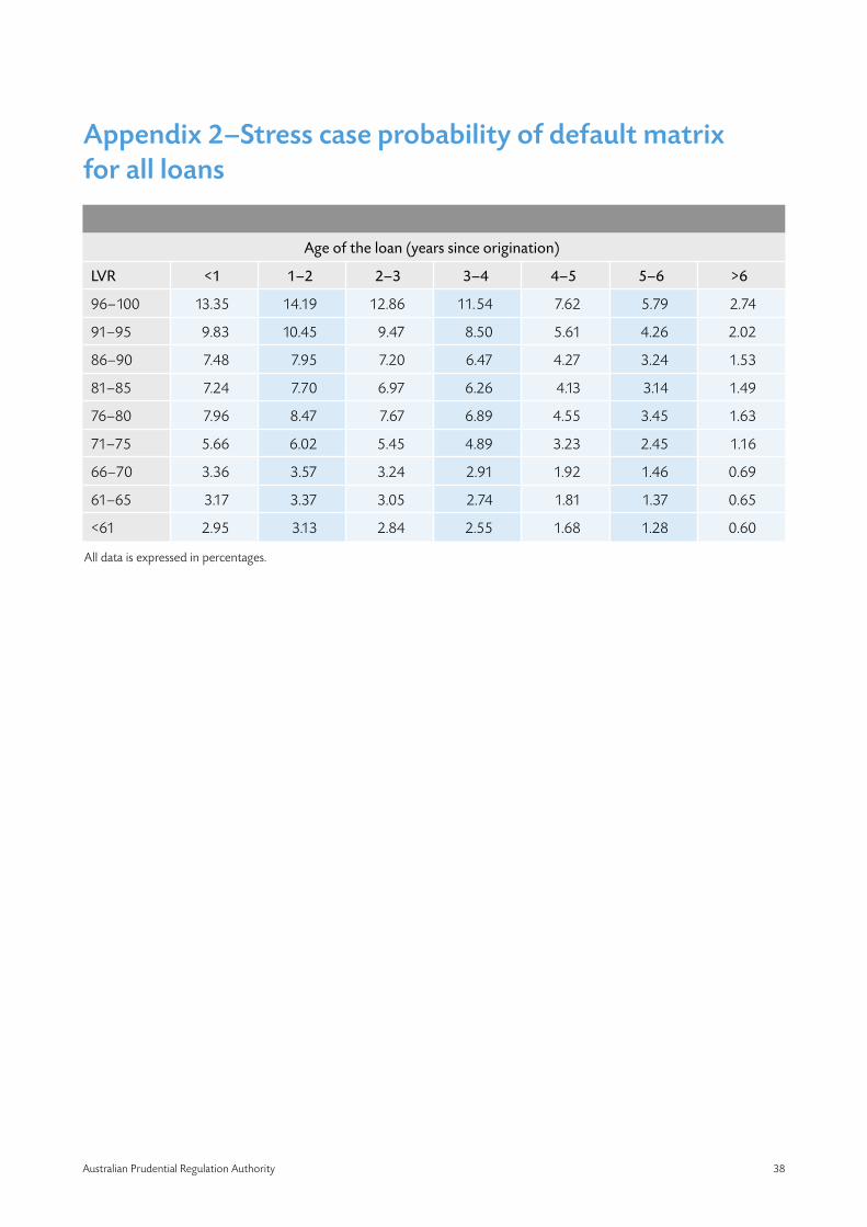
Australian Prudential Regulation Authority 38
Age of the loan (years since origination)
LVR <1 1–2 2–3 3–4 4–5 5–6 >6
96–100 13.35 14.19 12.86 11.54 7.62 5.79 2.74
91–95 9.83 10.45 9.47 8.50 5.61 4.26 2.02
86–90 7.48 7.95 7.20 6.47 4.27 3.24 1.53
81–85 7.24 7.70 6.97 6.26 4.13 3.14 1.49
76–80 7.96 8.47 7.67 6.89 4.55 3.45 1.63
71–75 5.66 6.02 5.45 4.89 3.23 2.45 1.16
66–70 3.36 3.57 3.24 2.91 1.92 1.46 0.69
61–65 3.17 3.37 3.05 2.74 1.81 1.37 0.65
<61 2.95 3.13 2.84 2.55 1.68 1.28 0.60
Appendix 2–Stress case probability of default matrix for all loans
All data is expressed in percentages.

Australian Prudential Regulation Authority 39
The model Y(t) = 1/[1+e–(a+ß x(t+1))] is estimated using non-linear least squares, where Y is the dependent variable (PD or LGD) and x is growth in real property prices. The reason that the dependent variable is determined at year t, whereas the independent variable is at t+1 relates to the nature of the PD and LGD series. The series are based on underwriting year, as opposed to claim year. This means that the PD (and LGD) is measured for the pool of loans that originated in year t, but that defaulted in subsequent years.
Appendix 3—Regressions relating house prices to PD and LGD
Table A3.1 Logistic regressions relating house price growth to PD and LGD
Variable Probability of default Loss-given-default
Constant -4.4762 (-32.42)
-1.2889 (-28.23)
House price growth -5.3135 (-2.34)
-1.6703 (-2.63)
Adjusted R2 0.2217 0.2453
Implied dependent variable for 30 per cent drop in house prices
5.3% 31.3%
t-statistics in parentheses. ***, ** represents significance at the 99% and 95% confidence levels respectively.
*** ***
** **

Australian Prudential Regulation Authority 40
Appendix 4–Risk profile and stress test results
(A, FQ, M, and TQ denote average, first quartile, median and third quartile respectively)
Figure A4.1 Median LVR (all loans)
% 90
85
80
75
70
65
60
55
50
% 100.0
90.0
80.0
70.0
60.0
50.0
40.0
30.0
20.0
10.0
0.0
Figure A4.2 Percentage of total loans that are mortgage insured
FQM
A
TQ
A

Australian Prudential Regulation Authority 41
(A, FQ, M, and TQ denote average, first quartile, median and third quartile respectively)
Figure A4.3 Percentage of total loans less than two years old
Figure A4.4 Estimated default rate
% 100.0
90.0
80.0
70.0
60.0
50.0
40.0
30.0
20.0
10.0
0.0
% 9.0
8.0
7.0
6.0
5.0
4.0
3.0
FQ
M
A
TQ
FQ
M A
TQ

Australian Prudential Regulation Authority 42
Figure A4.5 Forecast loss rate
Figure A4.6 Basis point decline in capital adequacy ratio
% 3.5
3.0
2.5
2.0
1.5
1.0
0.5
0.0
320
280
240
200
160
120
80
40
0
(A, FQ, M, and TQ denote average, first quartile, median and third quartile respectively)
FQ
MA TQ
FQ
M A
TQ

Australian Prudential Regulation Authority 43
1. Background research
• Project scoping (P)
• Literature review (P)
• Review of ADIs’ internal stress test models (P)
2. Develop model framework
• Project conceptualisation (P)
• Identify drivers of default and losses (P)
• Identify other factors e.g. mortgage insurance recoveries, resource costs (P)
3. Data collection
• Survey a sample of ADIs for PD data (P, I)
• Provide feedback to surveyed ADIs (P)
• On-site visits of LMIs (P, I, S)
4. Determine model parameters
• Formulate loss function (P)
• Determine base case scenario (P)
• Determine stress factors (P)
5. Build operational model
• Determine input and output requirements (P)
• Spreadsheet design (P)
• Validation checks (P)
6. Supervisor training and rollout
• Nationwide training of more than 100 supervisors (P)
• Brief regulatory and industry bodies (P)
• Distribute data request to 120 ADIs (S)
7. Data submission
• Receive data from ADIs (S)
• Validate data (S)
Appendix 5–Project phases and responsibilities
( ) denotes primary responsibility P = Project team S = Supervisors I = Institutions O = Other

Australian Prudential Regulation Authority 44
8. Perform stress test
• Input data (S)
• Select parameters and scenarios (S)
• Record findings and comments (S)
9. Analysis and collation of results
• Identify key prudential performance measures (P)
• Peer group analysis (P)
• Benchmarking (P)
• Internal discussion forum on stress test results (S, P)
10. Individual entity feedback
• Distribute project summary report (P)
• Distribute ADI stress test results (P)
• Distribute a letter highlighting ADI-specific strengths and weaknesses (P)
11. Public dissemination of findings
• Media release (O, P)
• Chairman’s address to industry (O, P)
12. Supervisory action and follow up
• Supervisory action matrix (P)
• Schedule on-site visits to poor performing ADIs (S)
• Raise internal capital targets (S)
• Identify industry wide issues e.g. reliance on LMIs, poor data systems (P)
• Scope follow-up projects (P, O)
( ) denotes primary responsibility P = Project team S = Supervisors I = Institutions O = Other

Australian Prudential Regulation Authority 45
% 3.5
3.0
2.5
2.0
1.5
1.0
0.5
0.0
UK Mortgage Arrears (Peak: 1992)
Queensland (Peak: 1987)
APRA LMI Model
Years (relative to peak)
-7 -6 -5 -4 -3 -2 -1 0 1 2 3 4 5 6 7
% 3.5
3.0
2.5
2.0
1.5
1.0
0.5
0.0
UK mortgage arrears (six months or more) is available from the Council of Mortgage Lenders. The Queensland claim data is based on data published by Australian LMIs and is based on the 1987 claim year (that is claims made on LMIs in 1987, irrespective of the year in which the policies were originated). The APRA LMI model depicts the maximum event retention capital requirement for Australian LMIs proposed by APRA in 2005, which as a rough approximation accounts for 80 to 90 per cent of an individual LMI's overall minimum capital requirement.
Appendix 6—Historical stress events

Australian Prudential Regulation Authority 46
Appendix 7—Regression summary of the stress test model
The model Y = 1 / [1+e–(a+ßX))] is estimated using nonlinear least squares, where the dependent variable is the estimated loss rate from the stress test and X is a vector of explanatory variables. The model is estimated using a cross sectional sample of 120 ADIs that participated in the stress test. SIZE is the dollar value of the housing loan portfolio, INVEST is the
***, **, * represents significance at the 99, 95, and 90 per cent and 95 per cent confidence levels respectively.
Coefficient t-Stat
CONSTANT -4.705 -24.08
Ln (SIZE) -0.035 -3.06
INVEST 0.260 2.35
LVR 61–70 -0.649 -1.38
LVR 71–80 1.980 9.67
LVR 81–90 2.930 11.67
LVR >90 3.343 9.33
AGE 1–2 -0.623 -2.63
AGE 2–3 0.260 0.57
AGE 3-4 1.401 2.09
AGE 4–5 -1.260 -3.29
AGE 5–6 -1.563 -1.781
AGE >6 -1.064 -2.69
LMI -1.874 -12.63
OP -0.141 -1.01
LARGE 0.722 5.53
Adjusted R squared 0.802
***
***
**
***
***
***
***
**
***
*
**
***
***
percentage of loans that are investment loans, LMI is the percentage of loans that are mortgage insured, OP is the percentage of mortgage insured loans written under open policy, LARGE is the percentage of large loans, LVR XX-YY is the percentage of loans with an LVR between XX and YY per cent, and AGE X-Y is the percentage of loans within the age range of X to Y.

Australian Prudential Regulation Authority 47
Ambrose, B. W., Buttimer, R., and T. Thibodeau (2001), ‘A New Spin on the Jumbo/Conforming Loan
Rate Differential’, Journal of Real Estate Finance and Economic, 23:3, 309–335.
Australian Prudential Regulation Authority (2005a), Prudential Supervision of Lenders Mortgage Insurance:
Amendments to Proposed Reforms.
Australian Prudential Regulation Authority (2005b), Implementation of the Basel II Capital Framework, Standardised Approach to Credit Risk, Discussion Paper, April.
Berry, M., Dalton, T., Engels, B. and K. Whiting (1999), Falling Out of Home Ownership, Mortgage Arrears and
Defaults in Australia, The Unviersity of Queensland.
Boss, M. (2002), ‘A Macroeconomic Credit Risk Model for Stress
Testing the Austrian Credit Portfolio’, Financial Stability Review, December 2002, 64–82, National Bank of Austria.
Calem, P.S. and M. LaCour-Little (2004), ‘Risk-based Capital Requirements for Mortgage
Loans’, Journal of Banking and Finance, 28, 647–672.
Campbell, T. and J. K. Dietrich (1983), ‘The Determinants of Default on insured
conventional Residential Mortgage Loans’, The Journal of Finance, Vol. XXXVIII (5), 1569-1581.
Esho, N. and A. Liaw (2002), Should the Capital Requirement on Housing Lending be
Reduced? Evidence from Australian Banks, Australian Prudential Regulation Authority, Working Paper, June 2002.
FDIC (1997), History of the Eighties-Lessons for the Future.
References
Helbling, T. and M. Terrones, (2003), ‘Real and Financial Effect of Bursting Asset Price
Bubbles’, in World Economic Outlook, Chapter II, When Bubbles Burst, IMF, pp. 61–94.
Insurance Council of Australia, LMI Standing Committee (November 2001), Australian LMI industry Historical Experience.
Klopfer, E. (2002), ‘A Mortgage Insurer’s Look at Basel II and
Residential Mortgage Credit Risk’, Housing Finance International, 17 (1), 22–32.
Laker, J. (2003), The Resilience of Housing Loan Portfolios—APRA’s
‘stress test’, http://www.apra.gov.au/speeches/03_20.cfm
Office of Federal Housing Enterprises Organisation (2003),
Risk-Based Capital Regulation, Amended Final Rule, February 13.
Reserve Bank of Australia, (2004), Financial Stability Review, September 2004.
Salas, V. and J. Saurina (2002), ‘Credit Risk in Two Institutional Settings: Spanish
Commercial and Savings Banks’, Journal of Financial Services Research, 22:3, 203–224.
Schwartz, A. J. (2001). Asset Price Inflation and Monetary Policy, Paper
presented at the Annual Meeting of the American Financial Association, New Orleans, 7 January.
Sorge, M. (2004), Stress-testing Financial Systems: An Overview of Current
Methodologies, BIS Working Papers, No 165.

Telephone 1300 13 10 60
Email [email protected]
Web site www.apra.gov.au
Mail GPO Box 9836 in all capital cities (except Hobart and Darwin)