Journal of Glaciology, Vol. 32, No. Ill, 1986

STRESS-GRADIENT COUPLING IN GLACIER FLOW: II. LONGITUDINAL AVERAGING IN THE FLOW RESPONSE

TO SMALL PERTURBATIONS IN ICE THICKNESS AND SURFACE SLOPE*

By K EITH A. ECHEL:-.lEYERtand BARCLAY KAMB

(Division of Geological and Planetary Sciences. California Institute of Technology. Pasadena. California 91125, U .S.A.)

ABSTRACT. As a result of the coupling effects of longitudinal stress gradients, the perturbations flu in glacier-flow velocity that result from longitudinally varying perturbations in ice thickness M and surface slope t:.a. are determined by a weighted longitudinal average of ~hM and ~~a., where ~h and ~a. are "influence coefficients" that control the size of the contributions made by local M and t:.a. to the flow increment in the longitudinal average. The values of ~h and ~a. depend on effects of longitudinal stress and velocity gradients in the unperturbed datum state. If the datum state is an inclined slab in simple-shear flow, the longitudinal averaging solution for the flow perturbation is essentially that obtained previously (Kamb and Echelrneyer, 1985) with equivalent values for the longitudinal coupling length l and with ~h = n + I and ~a. + n, where 11 is the flow-law exponent. Calculation of the influence coefficients from flow data for Blue Glacier, Washington, indicates that in practice ~a. differs little from 11, whereas ~h can differ considerably from 11 + I. The weighting function in the longitudinal averaging integral, which is the Green's function for the longitudinal coupling equation for flow perturbations, can be approximated by an asymmetric exponential, whose asymmetry depends on two "asymmetry parameters" ll and o, where ll is the longitudinal gradient of I (= dl / dx). The asymmetric exponential has different coupling lengths l+ and l_ for the influences from up-stream and from down-stream on a given point of observation. If O/ ll is in the range 1.5-2.2, as expected for flow perturbations in glaciers or ice sheets in which the ice flux is not a strongly varying function of the longitudinal coordinate x, then, when dl / dx > 0, the down-stream coupling length l+ is longer than the up-stream coupling length •~ and vice versa when dl f dx < 0. Flow-, thickness- and slope-perturbation data for Blue Glacier, obtained by comparing the glacier in 1957-58 and 1977-78, require longitudinal averaging for reasonable interpretation. Analyzed on the basis of the longitudinal coupling theory, with 41 + 1.6 km up-stream, decreasing toward the terminus, the data indicate 11 to be about 2.5, if interpreted on the basis of a respo11se factor 1/J + 0.85 derived theoretically by Echelmeyer (unpublished) for the flow response to thickness perturbations in a channel of finite width. The data contain an apparent indication that the flow response to slope perturbations is distinctly smaller, in relation to the response to thickness perturbations, than is expected on a theoretical basis (i.e. ~a.l¢h + 11/ (n + I) for a slab). This probably indicates that the effective 1 is longer than can be tested directly with the available data set owing to its limited range in x.

•contribution No. 4099, Division of Geological and Planetary Sciences, California Institute of Technology, Pasadena, California 91125, U.S.A.

tPresent address: Geophysical Institute, University of Alaska, Fairbanks, Alaska 99775, U.S.A.

REsUME. Coup/age du gradient de contrainte dans /'ecoulemem des glaciers: fl. Allenuation longitudinale de Ia reponse de l'ecou/ement aux faibles perturbations d'epaisseur de glace et de pente de Ia surface. Comme resultat des effets de couplage des gradients de contrainte, les perturbations flu de vitesses d'ecoulement du glacier qui n!sultent des perturbations variables longitudinalement dans l'epaisseur de glace M et dans Ia pente de surface t:.cx, sont determinees par une ponderation longitudinale de Ia moyenne de ~hM et ¢~ex, ou ~h et ~a. soot des "coefficients d'influence" qui contrOlent !'importance des contributions produites par les variations locales M et t:.cx, a une augmentation d'ecoulement dans une moyenne longitudinale. Les valeurs de ~h et ¢a. dependent des effets des gradients de contraintes longitudinales et de vitesses par rapport a un etat repere non perturbe. Si l'etat de reference est une couche inclinee en ecoulement de cisaillement simple, Ia solution de moyenne longitudinale pour Ia perturbation d'ecoulement est essentiellement ceUe obtenue anterieurement (Kamb et Echelmeyer, 1986) avec des valeurs equivalentes pour Ia longueur 1 de couplage longitudinal et avec ~h = n + I et ~a. = n, ou n est l'exposant de Ia loi de fluage. Des calculs des coefficients d'influence a partir des donnees du Blue Glacier, Washington, indiquent qu'en pratique ¢a. ne differe que peu de n bien que ~h puisse s'ecarter considerablement de n + I. La fonction de ponder­ation dans l'integrale de moyenne longitudinale, qui est une fonction de Green pour equation de couplage longitudinal de perturbation d'ecoulement, peut-~tre approchee par une exponentielle asymetrique, dont l'asymetrie depend de deux "parametres d'asymetrie ll et o, ou ll est le gradient longi­tudinal de 1 (= dJ / dx). L'exponentielle asymetrique possede deux longueurs differentes de couplage 1+ e~ 1 pour !'influence d'amont et d'aval sur un pomt donne d'observation. Si of ll varie de I ,5 a 2,2, comme prevu pour des perturbations d'ecoulement dans des glaciers ou des nappes de glaces pour lesquels le flux de glace n'est pas une fonction etroitement lie a Ia coordonnee longitudinale x, alors, quand d1f dx > 0, Ia longeur de couplage aval 1 + est superieure a celle amont 1_, et vice versa quand dl / dx < 0. Les donnees des perturbations d'ecoulement, d'epaisseur et de pente, obtenues par comparaison des etats de 1957-58 a celui de 1977-78 necessitent un moyenage longitudinal pour une interpretation raisonnable. Analyses dans l'optique de Ia theorie de couplage longitudinal, avec 41 I ,6 km a l'amont et decroissant vers le front, les donnees conduisent a un n voisin de 2,5, dans le cas ou !'interpretation est conduite sur Ia base d'un facteur de reponse ojl = 0,85 obtenu theoriquement par Echelmeyer (non publie) pour Ia reponse de l'ecoulement aux perturbations dans un chenal de largeur non-infinie. Les donnees contiennent une indication apparente qui conduit a reponse d'ecoulement aux perturbations de pente nettement moindre par rapport a celle due aux perturbations d'epaisseur, que celle qui est attendue selon Ia theorie (c'est-a-dire: ~a.l~h = 11/ (n + 1) pour en plaque). Ceci indique probablement que Ia longueur effective 1 est plus grande que celle qui peut ~tre testee

285

Journal of Glaciology

directement sur les donnees disponibles compte tenu de leur domaine limite en x.

ZUSAMMENFASSUNG. Kopplung von Spannungsgradienten im Gletscherfluss: fl. Mittelung der Flussreaktion auf kleine Storwrgen der Eisdicke und der Oberfllichenneigung in Llingsrichtung. Als ein Ergebnis des Kopplungseffekts longi­tudinaler Spannungsgradienten werden die StOrungen l!.u in der Gletscherfliessgeschwindigkeit, die von longitudinal schwankenden StOrungen der Eisdicke 6Jr und der Ober­fl!chenneigung l!.a verursacht werden, durch ein gewichtetes, longitudinales Mittel von 4>h6Jr und 4>~a bestimmt, wobei 4>h und 4>a "Einflusskoeffizienten" bedeuten, die das Ausmass der Beitr!ge durch lokale 6Jr und t.a zum Flussinkrement im longitudinalen Mittel regeln. Die Werte von 4>h und 4>a h!ngen von Auswirkungen der Uingsspannung und Geschwindigkeitsgradienten im ungestOrten Ausgangszustand ab. \Venn der Ausgangszustand eine gene igte Tafel mit einfachem Scherfluss ist, stimmt die longitudinal mittelnde LOsung f!ir die FlussstOrungen im wesentlichen mit der iiberein, die bereits f riiher (Kamb und Echelmeyer, 1986) erhalten wurde, jedoch mit !quivalenten Werten f!ir die longitudinale Kopplungsl!nge J und mit 4>h = n + I und 4>a = n. wobei n den Exponenten des Fliessgesetzes bedeutet. Die Berechnung der Einflusskoeffizienten aus Fliessdaten fiir den Blue Glacier, Washington, zeigt, dass in der Praltis 4>a our wenig von n verschieden ist, wlihrend 4>h betra.chtlich von n + I abweichen kann. Die G ewichtsfunktion im longi­tudinal mittelnden Integral, die Green's Funktion fiir die longitudinale Kopplungsgleichung fiir FlussstOrungen ist,

1. INTRODUCTION

In Part I (Kamb and Echelmeyer, 1986[b]) we showed that an approximate treatment of the role of longitudinal stress gradients in glacier flow gives a semi-quantitative description of how the influences of local thickness and surface slope of an ice mass are effectively averaged longi tudinally to drive the actual flow. This treatment, based on a perturbation approach that linearizes the basic flow­coupling equation (Part I , equation (8), hereafter referenced as equation (1-8)) so as to give simple, comprehensible results, is developed into a general description of the flow of ice masses, under the approximation that longitudinal variations in flow are calculable as perturbations from an overall average flow.

The perturbation approach can be used with greater exactness and rigor to treat small perturbations in flow that are caused by small changes in ice thickness and surface slope of the sort that develop in a glacier as a result of climatic change or during the gradual recovery and build-up after a surge. A manifestation of the effect of longitudinal stress gradients in this context is seen in the conclusions that Echelmeyer (unpublished) reached concerning observed perturbations in the flow of Blue Glacier (Washington) due to a secular change in the ice surface: the flow perturbations correlate much better with longitudinally averaged thkkness and slope changes than with local values. Longitudinal coupling theory is needed to provide a proper framework for interpreting perturbation-response measure­ments of this type so as to yield information on glacier­flow rheology.

In this paper (Part II), which is based on Echelmeyer (unpublished, p. 133-50), we develop a perturbation treatment that shows how longitudinal stress gradients affect the flow response of a glacier or ice sheet to small thickness and slope changes from an original datum state in which longitudinal variations in flow are already present. The dil ferential equation for the longitudinally coupled perturbations, obtained in section 2, is solved in section 3, and the result is applied to field data from Blue Glacier in section 4.

286

kann durch einen asymmetrischen Exponentialausdruck angenlihert werden, dessen Asymmetrie von zwei • Asymmetrie-Parametern" 1J. und o abMngt, wobei 1J. den longitudinalen Gradienten von J (= dJ / dx) darste llt. Der asymmetrische Exponentialausdruck hat unterschiedliche Kopplungsllingen I+ und •- fiir d ie Einfliisse von stromauf­w!rts und stromabw!rts auf einen bestimmten Beobachtungsort. Wenn O/ IJ. im Bereich von 1,5-2,2 liegt, wie man fiir FliessstOrungen in Gletschern oder Eisdecken erwarten kann, in denen der Einfluss nicht stark mit der Uingskoordinate x schwankt, und wenn dJ / dx > 0, dann ist die K opplungsllinge J+ stromabw!rts Hinger als •~ das umgekehrte gilt, wenn dl / dx < 0. Daten fiir Fluss- , Dicke­und NeigungsstOrungen am Blue Glacier, die aus Yergleichen des Gletschers in den Perioden 1957/ 58 und 1977/ 78 gewonnen wurden, erfordern longitudinale Mittelung, wenn sie verniinftig interpretiert werden sollen. Bei einer Analyse auf der Basis der Jongitudinalen K opplungstheorie mit 41 = 1,6 km stromaufwlirts, abnehmend gegen das Gletscherende, ergeben die Daten fiir n einen Wert von etwa 2,5; der Interpretation liegt ein Reaktionsfak/Or rJi = 0,85 zugrunde, der theoretisch von Echelmeyer (unverOffentlicht) fiir d ie Flussreaktion auf DickestOrungen in einem Kana! von begrenzter Weite hergeleitet wurde. Die Daten enthalten offensichtlich einen Hinweis darauf, dass die Flussreaktion auf NeigungsstOrungen im Vergleich zu der auf DickestOrungen deutlich kleiner ist, als man theoretisch erwarten kann (d.h. ~af4>h = n/(n +I) fiir eine Platte). Dies Jlisst vermuten, dass die effektive L!nge I grOsser ist als der mit den verf!igbaren Daten bestirnmbare Wert; der Bereich in x erscheint dafiir zu beschr!nkt.

2. LONGITUDlNAL COUPLING OF PERTURBATIONS IN ICE THICKNESS AND SURFACE SLOPE

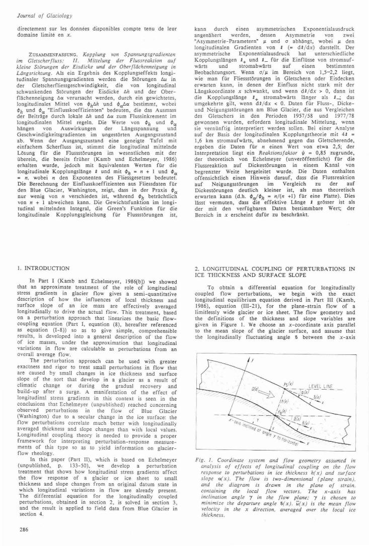
To obtain a differential equation for longitudinally coupled flow perturbations, we begin with the exact longitudinal equilibrium equation derived in Part 1H (Kamb, 1986), equation (lll-21), for the plane-strain flow of a limitlessly wide glacier or ice sheet. The flow geometry and the definitions of the thickness and slope variables are given in Figure I . We choose an x-coordinate axis parallel to the mean slope of the glacier surface, and assume that the longitudinally fluctuating angle 6 between the x-axis

Fig. I . Coordinare system and flow geomerry assumed in analysis of effects of longitudinal coupling on the flow response to perrurbations in ice thickness h( x ) and surface slope a( x ) . The flow is rwo-dimensional ( plane strain ). and the diagram is drawn in rhe plane of strain. conramurg the local flow vectors. The x-axis has inclination angle 1 in rhe flow plane; 1 is chosen ro minimize rhe departure angle 6{ x ) . li( x ) is the mean flow velocity in the x direction , averaged over the local ice thickness.

and the local surface slope can in this way be made small enough that terms of order 62 and higher in equation (Ill-21) can be neglected. We further assume that the longi­tudinal surface curvature is small enough that hda/ dx - 6 so that the curvature term in equation (HI-21) can be neglected, and that there is no basal sliding, so that o8 ' = 0 in equation (III-21 ). The equilibrium equation then reduces to

% d -(I + 2sin 8)T 8 = pghsina + 2-;-{hT~xl + T dx

(I)

where T 8 is basal shear stress, h is ice thickness, a is local surface slope, 8 is local bed slope relative to the x-axis, T~x is the "vertically" averaged longitudinal stress deviator in equation (JII-2), and T is as defined in equation (III-3).

Following the approach in Part I, section 2, we introduce two basic relationships between the y-averaged ~ow velocity ii and the stresses: I . T~x = 2i!dii/ dx, where 'I is the y-averaged effective longitudinal viscosity defined in equation (1-6). 2. A relation between T 8 and ii, for which we here take, in place of equation (1-l ), the more general form in equation (1-31), involving the effective shear viscosity 11 defined in equation (I-30): T 8 = 311ii/ h.

Echelmeyer and Kamb: Stress-gradient coupling in glacier flow

recognizing that the n' so defined is not necessarily the ex­ponent n in the flow law, because of the complicated functional form of 11 involving its dependence on dii/dx as well as on iij h. Because of this dependence, n' in Equation (3b) can be a function of x. We nevertheless expect that in normal glacier-flow situations the 11' defined by Equation (3b) will not depart greatly from the flow-law exponent.

The partial derivative symbols in Equations (3a) and (3b) give recognition that in principle, as noted above, 11 depends not only on T 8 but also on du/ dx. With this recognized, in principle there should be added to Equation (3a) a "cross term" containing the effect of the perturbation du/dx on the quantity 11uj h. We have, however, omitted this term, in the spirit of equations (1-1) and (I-9), which assume that the shear flow is so strongly dominated by the shear stresses (measured by T 8 ) that the effect of a small perturbation in longitudinal strain-rate can be neglected. The inclusion of the "cross term" leads to numerous small complications and also to an interesting effect that is, however, not due to stress-gradient coupling per se and is therefore beyond the scope of the treatment here; it will be developed in a separate paper.

To lowest order in the perturbations, we obtain from Equation (2), after cancelling the datum-state terms that separately satisfy Equation (2) exactly,

-4- h 'l =.l+'l==n +hi!:::il... d [ [- du dii ) du l dx 0 0 dx 1 dx 1 0 dx

Both i) and 11 are in general complicated functions of both iijh and duj dx, although in limiting cases they reduce to the simple forms represented by equations (I-1) and (1-7). Putting the above relationships into Equation ( I), we obtain the basic flow-coupling equation

d [ _&] 2 ii --4 - h'l- + (I+ 2sin 8)tr - = pghsina + T . dx dx h

(2)

We now introduce small perturbations about an original datum state that satisfies Equation (2): h = h0 + hl' ii = ii0 + u1, a = ~ + a 1, 8 • 80 + 131 , i) = ii0 + 'll' and T ~ T

0 + T

1, where subscript o designates the datum state and

1 the perturbations. The perturbation in 9 is designated 131 because 1 is held fixed, so that a change in 8 is the same as a change in bed slope B; such a change would come into consideration if we wanted to compare the flows expected over two beds that differed slightly from one another.

In carrying out the perturbation of the function 1lii/h, we write

11- - T l +~ _..-u ( BlnT.,, ~u, ~J] h - 0 8ln(Ujh)o -

0 h

0

(3a)

where T 0

is the unperturbed basal shear stress. Equation (3a) is a generalization of equation (1-9), in which the derivative 8lnT afBin(ii/ h), the slope of the logarithmic relation between ii! h and T 8 under the conditions of the datum state (represented by the symbol I Q in Equation (3a)), takes the place of the 1/ n in Equauon (I-9). The representation of T 8 in Equation (3a) as a function of the velocity-thickness ratio ii/ h is consistent with the form of equations (1-30) and (1-31) as well as with equation ([-1), and it also has an empirical basis (Raymond, 1978, p. 812). We will here put•

n

BloT B

81n(Uj h) [ 8ln1l I )-1 = 1----BinT 8 o '

(3b)

*The right-hand equality is derived from lnT 8 = In31l + ln(ii/ h) by taking differentials and solving for the ratio dinT 8 / dln(ii/ h) in terms of dlnfl/ dlnT 8 .

(4)

The way in which the viscosity perturbation 111 is coupled to the flow perturbation u1 can in principle be cal­culated from equations (I-6) and (l-22). In the limiting case where ii is dominated by the longitudinal strain-rate and the relationship in equation (1-6) simplifies to equation (I- 7), it follows by differentiating equation (1-7) that

(Sa)

and thus

(Sb)

The dependence of ii on du/dx is weakened, relative to that indicated by equation (I-7), when the effects of shear stresses, related to non-zero T 8 , are brought into consider­ation. This weakening is seen, for example, in the fact that as ~ increases, the magnitude of the slope of the curves of 'I versus du/ dx in figure 3 of Part I decreases. We will allow the weakening to be represented by replacing n in Equation (Sa) by a quantity n • smaller than n, in the range I ' n • ' n. (When n • = I, '11 • 0 in Equation (Sa), which is the limiting case where du1/ dx has a negligible effect on ii.) The n • so introduced is analogous to the n' in Equation (3b) in that it represents the slope of the differential relation between perturbations in longitudinal strain-rate and stress deviator under the conditions of the datum state. In fact,

[ 8Inii ] -1

n • = I+ Sin(du/ dx) lo

(5c)

which shows formally the analogy with n' in Equation (3b).* Although n • can thus be a function of x, we assume

• Equation (Sc) is derived by solving Equation (Sb) for n (renamed n "), substituting the first relation for 111 in Equation (Sa), gathering factors to form the logarithmic derivative, and cancelling the common factor n0du1/ dx in numerator and denominator.

287

Journal of Glaciology

that it is slowly enough varying that its x-derivative can be ignored.

The partial derivative symbols in EQuation (5c) are written in recognition that in general 'ii is a function not only of dU/dx but also of T 8 • In writing the perturbation in the form of EQuation (5b), we make the assumption , analogous to what is done in EQuation (3a), that the main perturbing effect on the longitudinal stress is the change in longitudinal strain-rate du/dx. and we omit the effect of perturbations in T 8 on the longitudinal stress, which would in principle appear as a "cross term• in addition. Inclusion of this term leads to numerous small complications that will be treated in the subseQuent paper mentioned above.

The formulation of the perturbations in EQuations (3) and (5) frees the treatment here of the approximations that would be introduced by assuming the simple flow relation­ships in EQuations (I-I) and (1-7). This can be done because in the small-perturbation treatment we need only the derivatives, at datum-state conditions, of the flow relationships. The cost of doing it is the appearance of the parameters n' and n •, which are not necessarily the same as the flow-Jaw exponent n, and which may give the treatment an empirical flavor, although n' and n • could in

This reflects a key difference between the two perturbation treatments, in Part I the perturbation being treated in such a way that an unperturbed Quantity n0 never appears. Except for this non-trivial difference, and except for the possible difference between n' and n, the present treatment of longitudinally coupled flow perturbations from a general datum state reduces exactly to the treatment in Part I under the conditions stated above.

and

With the definitions

0 = I d _ -I- In (h ll ) 2 dx 0 0

( I I)

(12)

which are similar to eQuations (1-11) and (1-12), and with neglect of the effects of the T1 term (see Part IV; Kamb and Echelmeyer, 1986[a]), EQuation (6) can be written

-•2 .::....::l... - 2ol ..::=.1. - :..:..1.. ~ d2u du [ h ]

• 2 + ul = uo ~h + ~ . - ~ca . dx dx h

0 a sm~ ., 1 (13)

principle be calculated from EQuations (3b) and (5c). In addition, this approach brings out explicitly a limitation on the theory that is involved in omitting the "cross terms• in EQuations (3b) and (4a) as discussed above.

If now we introduce EQuation (5a) into EQuation (4), and collect terms, re-arrange, multiply through by n' / T and by 1/ ( I + 2sin2e0 ), and utilize the relation~ dh1/ dx z -a-. + a1 and T 0 = pgh0sin~ (which simply represents the local shear stress T 0 in terms of an effective slope ~. as in Part I, section 7), we obtain

(6)

where

(7)

(8)

(9)

2n' _ 4n''ii0 ~ ~a • --sb in2e0 bT0 dx ( 10)

These relations are valid for all angles ~ and e0

.

The "influence coefficients" ~h• 4>cr and ~13 in EQuations (8)-iiO) govern the effects of the perturbations hl' ~· and a1 on the flow via their contributions to the r ight- hand side of EQuation (6). Their values depend on the local stress and flow conditions in the datum state, as well as on n' , and they are thus functions of x.

The influence coefficients 4>h and 4> reduce to 4>h = I + n' and 4>a = n' for the datu~ state of the perturbation treatment in Part I (the inclined slab), for which o:0 and e0 are small, all longitudinal derivatives are zero, and ~ • a 0 . In that treatment we replace n' with n, because we use eQuation (l-1) instead of EQuations (3a) and (3b). In that treatment also, the analog of the perturbed flow-coupling EQuation (6) lacks the n • in the denominator of the term on the far left, and has 'ii instead of 71

0 there.

288

This differential eQuation has the same basic form as eQuation (1-13). The meaning of the parameters I and o is the same as discussed in Part I, sections 3 and 5. Because the factor n • in the denominator of EQuation (II) may be in the range I to n, as noted above, the averaging length scale given by EQuation (I I) can be somewhat shorter than that from eQuation (I-ll), evaluated in Part I, section 5.

3. SOLUTION OF DIFFERENTIAL EQUATION FOR LONGITUDINALLY COUPLED FLOW PERTURBATIONS: ROLE OF ASYMMETRlC LONGITUDINAL AVERAGING

The solution of Equation ( 13) by the Green's function method used to solve equation (1-13) in Part I reveals some distinct differences that arise because of the fact that while u0 and T 0 in equation (1-11 ) are constants at the rough level of approximation used in Part I, in Equation (II) they (and also b and possible n' and n ") are here functions of x, being features of a datum state that in general involves longitudinal variations in flow and stresses. Because of this, the parameter o, from Equation (12), is no longer equal to the parameter 1J. defined by

IJ. dl

dx

dinS 0 + --1

dx (14)

where S = An• u9t bn "T 0 • Detailed features of the solution for o = IJ., obta1ned in the Appendix to Part I, are modified when o ~ IJ..

The modified solutions, for o ~ IJ., are developed in the Appendix to this paper, following an initial section in which the relationship between o and 1J. for situations of interest is established. The results of the Appendix are summarized below, and their implications discussed.

The Green's functions G(x I x' ), obtained in the Appendix (section A.2} and discussed in sections A.3-A.6, serve to generate the solution of Equation ( 13) by means of the "longitudinal averaging integral"

ul(x) = r2 F(x' )G(x I x' }dx'

xl

( I 5)

where x 1 and x2 locate the head and terminus of the glacier, and where, from EQuation (13),

(16)

(In Equation ( 15) we replace the "source point" coordinate ~

of the Appendix by x' , following the notation of Part I, section 3.) The Green's function thus acts as a weighting function in the longitudinal average of the effects of the perturbation h 1 , a 1 , and a1 on the flow response. In general, the Green's function for longitudinally varying J and non-zero o can be approximated by an asymmetric exponential as in Equation (A-23)

where

(17b)

and where the - sign applies for x' < x, the + sign for x' ~ x. This is an exponential with different scale lengths (or coupling lengths) up-stream (x' < x) and down-stream (x' > x) from the "point of observation• at x . Since the amount and type of asymmetry are controlled by JJ. and o, we may call these the "asymmetry parameters". For IL = o = 0, Equation (17) is the exact Green's function and is the simple symmetric exponential, with coupling length J , used in Part I (equation (1-15)). The parameter v in Equation ( 17) can be chosen to make Equation ( 17) represent as well as possible the exact Green's functions for IL ~ 0, o ~ 0. For linearly varying J(x) with O/ JL = I , the case treated in the Appendix to Part I, the Green's function is approximately symmetric, and v * 0 is a good choice, so that J+ = ._ = l(x). For O/ JL = 3/ 2, which is thought to be the condition most generally applicable to flow perturbations, there is distinct asymmetry (1+ ~ J_), and v "' +D.7 is a good choice. From Equation (17b), and in agreement with intuition, the down-stream coupling length J+ is longer than the up-stream coupling length R_ if IL > 0 (J increasing down-stream), and vice versa if IL < 0. For o/ JJ. > 3/ 2, the amount of asymmetry increases; thus for o/ JL = 9/ 4, the choice v * +1.2 in Equation (17) is good. For lJ. - 0, with o ~ 0, Equation (17) becomes the exact Green's function, with VJJ. replaced by o .

The ratio O/ JJ. • 3/ 2 applies for flow perturbations of a wide ice sheet under conditions where the ice flux in the datum state is longitudinally constant (or nearly enough so), and in which longitudinal vanat10ns in J are not predominantly controlled by longitudinal variations in n

0.

For flow in a channel of finite width, of parabolic cross­section, the constant ice-flow condition corresponds to O/ JL = 9/ 4, hence the asymmetry in the Green's function tends to be greater for valley glaciers than for wide ice sheets, for a given value of J.l..

In asymmetric longitudinal averaging, with the use of Equation (17) in the integral in Equation (15), the practical range of integration (the "averaging interval") can reasonably be taken to be x - 21_ ' x' ' x + 21+, in accordance with the form of the exponential, as illustrated in Figure 2 ("averaging length" 2J+ + 2L "' 4J). (To do this, the right side of Equation (17a) should be multiplied by the additional scaling factor (I - e-2)" 1.) Although 1 t in Equation (17b) is a function of x via J(x) in Equation (17), in the integration in Equation (15) it is a constant, except for the switch from I_ to '+ as x' passes through x .

Figure 2 shows qualitatively the anticipated pattern of weighting-function asymmetry along the length of a glacier, based on the expectation that I will decrease as the terminus and head of the glacier are approached and also on going into ice falls.

From Equation (A-23b), the exact Green's function for the case where J(x) in Equation ( 13) is a linear function of x and where o = constant = (3/ 2)JJ. is

G(xix') 2t(x) ~

(18)

in which the + sign applies for x' ' x, the - sign for

Echelmeyer and Kamb: Slress-gradient coupling in glacier flow

Fig . 2. SchemaLic representalion of asymmetric weighting funclions for longiLUdinal averaging of lhe elfecls of perturbalions in ice lhickness and slope on 1he flow response. The scheme used is explained by lhe upper diagram. which shows a plo1 of lhe asymmetric weighling function in Equation ( 17) ( here designaLed W 1 as in Figure 12) as a funclion of x' around a parlicular "poinl of observaLion· x , for a particular choice of VJL ( • 0.55 ). In the lower diagram. such plots of W 1( x' ) are shown schematically around five points x1 .... x 5• The weighting for averaging around x

4 is approximalely sym'!"etrical,

while for the other points it is dislinctly asymmemcal; the diagram shows the sense of asymmetry expected near the head and terminus. and near an ice fall.

x' ~ x. (The actual sign of the exponent depends also on the sign of IL, as Equation ( 18) indicates.) The range of x' in Equation (18) is limited to ILX' ~ ILX - J(x). Since the approximate representation of Equation (18) by Equation (17} (with v = +D.7) becomes somewhat poor for JJ. ;o: I, Equation (18} should be used in Equation (15) under those conditions of rapid longitudinal variation of I and high asymmetry.

The function in Equation (18) is actually symmetric for x in the immediate vicinity of x; asymmetry as in Equation ( 17) develops progressively outward. The detailed features of the asymmetry are shown in Figures 8, 9, and 10. Figures 9 and 10 also show how well Equation (18} is approximated by the asymmetric exponential in Equation ( 17) with v taken as I.

The expectable extent of overall asymmetry, as measured by the ratios f~J and J_JJ, is shown by the values in Table I. They are calculated from Equation (17b), with v - I, for several values of JJ., which are based on

TABLE I. ASYMMETRICAL AVERAGING LENGTHS I_

AND J+

Calculated from Equations (17b) and (19) with v • I and 0/ JJ. - 3/2

l fho -(o:-6) IL J_jJ ·~· deg

2 2 0.023 0.98 1.02

2 5 0.058 0.94 1.06

2 10 0.118 0.89 1.12

2 20 0.243 0.79 1.27

6 I O.Q35 0.97 1.04

6 2 0.070 0.93 1.07

6 5 0.175 0.84 1.19

6 10 0.353 0.71 1.41

6 20 0.728 0.51 1.96

If a - a > 0 (IL < 0), the numbers in column 4 and 5 are

to be interchanged.

glacier geometry in terms of the "convergence angle" (a- a) c -tan-1(dh0 f dx}. For a given value of the ratio O/ IL, the longitudinal gradient of ice thickness dh0 / dx is related to ll by

289

Journal of Glaciology

(19}

which is obtained form Equation (12) with neglect of the contribution to o from dll0 1dx. The values in Table I are based on oi JJ. - 312. For l l h • 2, the practical upper limit of J1. is about 0.3, whereas for l l h • 6 (which seems possible on the basis of Part I, table I), we might encounter Jl. - I.

There are indications that the form of Green's function is only moderately sensitive to non-linearities in J(x), so that the weighting functions in Equations (18) or (17) are applicable in a practical way to actual situations where the longitudinal variations in J(x) are not strictly linear but do not depart too wildly from linearity. The effect of longitudinal variation in J1. can, on the basis of equation (IA-22), be taken into account in a rough way by replacing J in Equations ( 17) or ( 18) by

(20)

The practical approximate solution of Equation (13), obtained by combining Equations (15), (16), and (17) into a single formula based on the above discussion is

I JX2 - 1x' -x 11• F(x' )e *dx' (21) 2J/J +VJ1.2 X

1

where J ± is given by Equation (17b) and F(x) by Equation (16). In these formulae J1. • dl l dx.

The effects of the asymmetry in longitudinal averaging on the flow response u1(x) are likely to be small in general, first because J1. is probably in general small as noted above, and secondly because u 1 is not in general very sensitive to modest changes in the shape of the weighting function in Equation (15). However, an exception occurs in places where h0 decreases to low values so that F(x) has an exaggerated sensitivity to thickness perturbations via the h lh0 term in Equation (16). Such places are near the ends ot a glacier and near ice falls. The inordinate influence that such places would tend to exert via longitudinal coupling on the now response of adjacent, more "normal" parts of the glacier will tend to be suppressed and mitigated by the effects of asymmetric averaging, because the decrease in h0 toward these places will in general be reflected in a decrease in J toward them. The asymmetry of the weighting function in such situations, suggested in Figure 2, will tend to shield the flow response in adjacent parts of the glacier from the influence of these places where the extreme response conditions arise. However, very near the terminus the treatment here tends to fail for other reasons.

4. APPLICATION TO AN OBSERVED PERTURBATION IN GLACIER FLOW

From 1957 to 1977, Blue Glacier (Washington) increased in thickness by a few tens of meters. At the same time, there was a general decrease in surface slope, corresponding to a longitudinal gradient (a down-glacier increase) in the thickening. The combined effect of these changes was a marked increase, up to 40%, in the flow velocity. The changes have been documented by Echelmeyer (unpublished), building upon the basis laid in 1957-59 by Meier and others (1974). From the measured perturbations, a comparison can be made between the observed now response and the response expected from the slope and thickness perturbations with and without longitudinal averaging.

Figure 3a shows a plot of the observed u11h0

values in relation to the corresponding local perturbation h/ h

0 without longitudinal averaging. The values of the local per­turbations a/a0 are given alongside the plotted points in the figure. Throughout this discussion and in Figures 3-7 we use as our numerical measure of the perturbations u

11u

0,

290

{b) . -9 8

-2.8 . 20~

~ 10 ~

-48

-61 -8 .

-S6 -7.0

-10 0~---75----~,~0----~----~--~10~--~,~5----~20~--~

11,/110 1%) (li1/li0) {%)

Fig. 3. Flow perturbaJion daJa for Blue Glacier. ( a ) PerturbaJions in flow velocity u1/ u0 ( expressed as percentage change) are p/oued against the corresponding local perturbaJions in ice thickness h1/ h0 . The associated local perturbaJions in surface slope ~/a0, in per cent ( measured over a longitudinal interval of 350-500( m centered on each daJa locaJion ). are given alongside each daJa point. The perturbaJion quantllles are calculated logarithmically from the observed flow and surface profile in 1957-58 and 1977-78 as explained in the text. DaJa are from Echelmeyer (unpublished). ( b) Plot of perturbation data after performing symmetric longitudinal averaging of thickness and slope perturbations according to Equation ( 24 ), with averaging length 4 I • 1.6( km in Equation ( A-21 ) . The averaged values <a1; a0 ) are given , in per cent , alongside each daJa point.

~la0, and h11h0 the quantllles ln(u0 1u1), ln(a111a1), and ln(h111h1), where subscripts 1 and 11 refer to values measured in 1957-58 and 1977-79, respectively. We consider this to be the optimum way to handle perturbations that are not truly infinitesimal (see Echelmeyer, unpublished, section 5.1), and it avoids the ambiguity in the choice of u

0 that arises

if linear quantities such as (uu - u1)1u0 are used. The logarithmic pert urbation values are expressed in per cent.

In Figure 3a there is considerable scatter of the data points about a bi-linear regression line of the type

(22)

that would be expected for the response to small changes in thickness and slope for flow in a cylindrical channel without effects of longitudinal stress gradients (Echelmeyer, unpublished, p. 258). Here 't' is a response factor whose value depends on the shape of the channel cross-section and for Blue Glacier is approximately 0.85 (Echelmeyer, unpublished, p. 284). The scatter in Figure 3a is not so great as to obscure the existence of the expected regression of u1l u0 against h/h9 , but there is no detectable correlation of u1l u0 with the a 1taa values, which scatter widely.

The expected effect of longitudinal stress-gradient coupling in modifying Equation (22) is obtained by application of Equation (21 ). It can be written, for small ~.

(23)

where the angular brackets represent the weighted longitudinal averaging specified by the integral in Equation (~I ) and where_ the influence coefficients ¢1h and ¢Ia are g1ven by Equations (8) and (9). The response factor 'I' in Equation (23), which is not present in Equation {16), is introduced on the basis of the reasoning developed by Echelmeyer (unpublished, sections 9.2-9.4) for channels of finite width, leading to Equation (22). Inasmuch as Equation (21) describes perturbations u1 in the mean velocity ii, in applying Equation (23) to observed perturbations in the sur­face velocity u we assume that the two perturbations at any

point are the same, or are proportional as they are theoretically in simple-shear now.

lf, as a first step, we were to assume that the influence coefficients had the approximate values ¢h "' I + n and ~a "' n (as in the treatment in Part I) and for consistency were also to omit the distinction between ~ and aa (see section 2}. then the expected relation tn Equation (23), with 'I' taken as constant, would be

(24)

Figure 3b shows accordingly the result of replotting the data points after applying longitudinal averaging to the h/ho and a,_/a

0 values. The averaging is done with a symmetric

exponential weighting function (Equation (17 ) with IL = 0), for simplicity; the expected decrease in 1 near the terminus is represented by taking the averaging length to vary with x as follows: for x < 0.6 km, 41 = 1.6 km; 0.6 < x < 1.2 km, 4J = 1.2 km; x > 1.2 km, 41 = 0.8 km. !h~ variation in u0 under the integral sign in Equation (21) ts. tgnored. T_he averaged values <a1/aa >. in per cent, are gtven alongstde the data points in Figure 3b.

The replotting of the data in Figure 3b, with application of longitudinal averaging, reduces the scatter in t~e regression of u1/ u0 against <h/h0 >. by comparison with Ftgure 3a. The remaining scatter, other than that from observational error, should according to Equation (24) be due to variations in <a,./aa >. As a result of the longitudinal averaging, the variations in <a1/aa > are greatly reduced from the variations in the local values a / a , as the numbers in Figure 3 indicate. In Figur~ 0

3b, some correlation can be seen between the <atfa

0 > values and the

departures of the data points from the regression line drawn, the points with the algebraically larger <a,_/a > values tending to fall above the line and those with mo~e negati ve <a1/a0 > values below it, as expected from Equation (24). However, the extent of departure is only about one-third of what would be expected from Equation (24) with n • 3. The non-zero intercept of the regression line on the <utfu > axis in Figure 3b is a separate indication of the effect of slope change on the flow. If the regression line is not biased by a correlation between <atfaa > and <h/hQ >. the intercept can be interpreted as the flow perturbation resulting from the mean of the per_turb~tions <atfa0 > for all of the available data points, whtch IS -6.7%, from the numbers in Figure 3b. On this basis, the intercept value of -8.5% (Fig. 3b) corresponds to an n value (1.3) in Equation (24) that is again about one-third as large as what we would expect if n is the normal flow- law exponent. On the other hand, the slope of the regression line in Figure 3b corresponds to a "normal" value n ~ 2.7 if interpreted by Equation (24) with 'I' c 0.85.

A more refined level of consideration of the perturbation data is attained by using the actual values of the_ influen~e coefficients ~h and ~a in Equation ( 13}, whtch take tnto account the dependence on effects of longi­tudinal stress gradients in the datum state. From Equations (8) and (9) they can be written (for small a)

(25)

Echelmeyer and Kamb: Stress-gradient coupling in glacier flow

~a=n' (l+ja) (26)

where

(ij ~] 0 dx (27}

and

(28)

In Equations (25)-(28}, the quantities cos aa and b that appear in Equations (8) and (9} have been taken to be 1 for practical purposes. As in Part I, section 7, ~ in Equation (25) is the effective slope that relates to

0 the

unperturbed local basal shear stress via the relation T 0 • pgh0sin~. As indicated in equation (1-24}, ~ is essentially a weighted longitudinal average of aa· 0

To evaluate the effects of the datum state on the influence coefficients, we list in Table II the values of 'I' a0/~. j h• and j a for each of the data points for Blu~ Glacier (the center-line point of each transverse profile where u, h, and a were measured in 1957-58 and 1977-78}. The quantities jh and ja in Equations (27) and (28} are calculated from a curve u0 (x) based on the velocity values listed (which are for 1977-78}. and with ii

0 taken constant

at 5 bar a, which is about as low a value as seems possible, consistent with 1/ h "' 2 (see Part I, table I). From the numbers in Table II, it appears that j is commonly small enough to be disregarded. In contrast,a the values of j h are generally large enough to have a definite effect on the flow response to thickness perturbations. The variations in a0/~ are also large enough to affect the response appreciably via Equation (25).

If we define two variables U and n as follows

(29)

(30)

we can restate the relationship in Equation (23} in the simple form

U = n' n . (31}

To evaluate the perturbation data from Blue Glacier on the basis of Equation (31 }, the indicated longitudinal averages in Equations (29) and (30} are carried out with the a9!~. j h• and 'I' values in Table II, and the resulting pairs of perturbation quantities U and n, from Equations (29) and (30), are plotted as points in Figure 4b. The averaging is exponentially weighted, with both longitudinal variation and (near the terminus) asymmetry in coupling lengths J J as indicated in Table 11. For comparison, UL and nL ~el on local values of the perturbations and influence coefficients, without longitudinal averaging, are plotted in Figure 4a. The

T A BLE 11. DATUM-STATE EFFECTS ON INFLUENCE COEFFICIENTS FOR BLUE GLACIER

Prufile X uo aat~ jh ia y ·- '+ IL km em d- 1 km km

-0.33 15.3 1.06 -0.23 -0.01 (0.85) I -0.11 14.8 1.03 -0.15 0.00 0.85 0.4 0.4 0 II 0.15 14.3 0.90 0.31 0.00 0.77 0.4 0.4 0 G 0.34 15.2 0.95 -0.09 +0.01 0.81 0.4 0.4 0 F 0.51 15.6 1.06 0.08 +0.01 0.70 0.4 0.4 0 E 0.75 16.6 1.10 -0.63 0.00 0.89 0.3 0.3 0 D 0.97 14.6 1.22 0.16 +0.03 0.88 0.3 0.3 0 c 1.11 13.6 0.87 0.21 -0.02 0.84 0.3 0.2 -0.2 B 1.34 12.8 0.78 0.19 0.00 0.78 0.25 0.15 -0.25 A 1.40 13.2 1.00 0.10 0.01 (0.80}

291

Journal of Glacwlogy

cL­" -

-Of%.' I

r i

Fig. 4. Flow perturbation data for Blue Glacier ploued in terms of the perturbation variables U and n ( m per cem) according to the framework provided by longitudinal coupling theory in Equations ( 29)--{31 ) . The quantities UL and nL ploued in ( a ) are calculated according to the format of Equations ( 29) and ( 30) but without longitudinal averaging, while in (b). U and n are calculated with longitudinal averaging as specified in Equations ( 29) and {30) . The local values of '1', ao/~· and vh used in calculatmg n for the data points are listed in Table II. The longitudinal averaging parameters J ± are given in the text. The open c~rcle is the result of a symmetric longitudinal average with 4 1 • 1.0 km for the a-profile pomt. showing the sensitivity of this result to the choice of averaging parameters.

application of longitudinal averaging greatly improves the relationship among the data points in Figure 4b, converting a complete scatter into a tolerable regression between n and U values. However, the regression is not weU fitted by a straight line. Moreover, it does not pass through the origin, which violates a requirement of Equation (31 ). The cause of this anomaly can be traced, at least formally, to a relatively suppressed flow response to slope perturbations in relation to the response to thickness perturbations, a feature already discernible in the data in Figure 3b as discussed earlier. If we modify the perturbation quantity n in Equation (30) as follows

(32)

by introducing, ad hoc, a second response factor ~. for the effect of slope perturbations, then we find that the choice ~ 2 0.35 yields a reasonable regression line between U and n' (Fig. 5), passing through the origin. Its slope corresponds to n ' • 2.5. However, since we think, on a theoretical basis

25 •

2C

15 U(%)

10

10 15

n'(%l

Fig . 5. Blue Glacier perturbation da1a in terms of the modified variable n' in Equal ion ( 32 ). wi1h a slope- response faCior ~ • 0.35.

292

(Echelmeyer, unpublished, section 9.1), that ~ • I, we are reluctant to accept the above interpretation, with drastically reduced ~. as more than a formal explanation of the data.

An alternative formal explanation would be that for some unknown reason ja in Equation (30) consistently assumes a value of about -2/3; however, we see no way that this large, consistent value could arise from Equation (28), or from effects of the T 1 term in Equation (6) (see Part IV).

Probably a better conclusion is that the proper averaging length is longer than that used in the longitudinal averaging in Figures 3 and 4, so that the variations in <a.fa0 > are further suppressed. We cannot test this idea directly with averaging calculations, because the limited x range of the data set prevents meaningful averages with longer J .

However, the following considerations suggest that the idea has merit. Over the range of observation (-<l.3 ' x ' 1.3 km) the htfh0 values scatter around a linear trend in x (Fig. 6). If this trend were to continue outside the range of observation, symmetric longitudinal averages would give

-•}.5 \..'.::, l(i

.( (km)

Fig. 6. Variation of the perturbations h1j h0 and ~/a0 with longitudinal coordina1e x in Blue Glacier. The dashed line is a linear regression filled 10 the h1j h

0 values. Data from

Echelmeyer ( unpublished).

h1 / h0 values following this linear trend better and better as the averaging length is increased. At the same time, since a.Ja9 is approximately proportional to the longitudinal gradtent of h\/ h0 (as Figure 6 shows), longitudinal averaging will g1ve (a1/ fXo > values tending to a constant as the averaging length is increased. For a long enough averaging length, therefore, the u

1/ u

0 values should show a

response to h1/ h0 varying linearly along the length of the glacier, while the response to a.f~ should appear only as a constant shift, resulting from the constant value of the longitudinally averaged <atf~ >. In conformity with this expectation, a plot of utfu0 against htfh

0 (where 1ltfh

0 is

the value given by the linear trend in Figure 6 for each observation point x) shows a good linear regression (Fig. 7).• The slope of the line in Figure 7 (ignoring the point for profile B) corresponds to n E 4.1 (assuming 'f • 0.85),

• The point from farthest down-glacier (profile B) falls well above the regression line, doubtless because of the sharp up-swing in h1/ h0 values above the linear trend in Figure 6 for x > I .3 km, approaching the terminus. The influence of this up-swing is evident in Figure 3b, in which the corresponding point for profile B does not fall above the regression line; it is also suggested by the fact that the point for profile B in Figure 7 moves much closer to the regression line when plotted at the position of the local h.Jh0 value (open circle in Figure 7).

i

Fig. 7. Flow perturbation u1/ u0 for Bl~ Glacier plotted as a function of thickness perturbation h1/ h0 given by the linear trend in Figure 6 evaluated at the points of observation. The open circle is for the B-profile point, re-plotted at the local value of h1/ h0 • The regression line has slope 4.35 and ordinate intercept -14%.

and the intercept value (u1/ u0 • -14% at h1/h0 • 0) corres­ponds to n • 3.0 if for the constant average value (a1/eta > we take the actually measured average value ( a 1 )/ <eta> • -<1.6% over the interval of observation ~.33 ' x ' 1.34 km. These reasonable n values differ from those implied by Figure 3b, as discussed above, perhaps because of effects entering the longitudinal averaging integrals from outside the interval of direct observation. The outside data have to be based on estimates from topographic maps of relatively modest accuracy and are therefore much less reliable than the data from inside the interval. This is especially the case for B, the lowermost profile.

The rather reasonable behavior of the perturbation data in the treatment of Figure 7 might be interpreted as an indication that in Figure 6 the fluctuations of the a1/ a

0 values from a constant value and of the htfh0 values from a line of constant slope represent only observational error, except perhaps for the B-profile point. Although the assessment of observational error in relation to this possibility is too complicated and extensive an issue to enter

APPENDIX

SOLUTION OF DIFFERENTIAL EQUATION (13)

By B. KAMB and K.A. ECHELMEYER

A.l. RELATION BETWEEN o AND ji., AND BETWEEN hAND I

If the ratio 1/ h is (approximately) constant, so that 1/ h • 1.. "' 2, as suggested by the results in Part I, then, from Equations (12) and (14),

I 0 - 2

~In ~- 1 dx k 21L + v (A-1)

where v is a parameter defined, analogously to o, by

I dlnlf0 v - - (A-2)

2 dx

To the extent that longitudinal variations in • are

Echelm eyer and Kamb: Stress-grad1e111 coupling in glac1er flow

into here, this points up the fact that longitudinal (as well ~ lateral) averaging of the h1/h0 and ~leta data is helpful 10 suppressing noise due to observational error, as well as in taking into account the actual effects of stress gradients.

Because this paper is concerned with the framework for evaluating flow-perturbation data under the influence of effects of longitudinal stress gradients rather than with the interpretation of the results themselves, we shall defer a full discussion of the data and their interpretation to a separate paper. It is, however, clear from the foregoing discussion that in interpreting such data it is helpful to use longitudinal coupling theory, and that, indeed, without bringing in the effects of longitudinal averaging, especially its damping of longitudinal variations in the local surface­slope perturbation ~, it would not be possible to make good sense out of the data for Blue Glacier.

ACKNOWLEDGEMENTS

This work was done under the support of National Science Foundation grants EAR-50-08329 and DPP-82-09824. We thank the U.S. National Park Service for permission to collect the field data in section 4.

REFERENCES

Echelmeyer, K .A. Unpublished. Response of Blue Glacier to a perturbation in ice thickness - theory and observation. [Ph.D. thesis, California Institute of Technology, Pasadena, 1983.]

Kamb, B. 1986. Stress-gradient coupling in glacier flow: Ill. Exact longitudinal equilibrium equation. Journal of Glaciology, Vol. 32, No. 112.

Kamb, B., and Echelmeyer, K.A. 1986[a]. Stress-grad ient coupling in glacier flow: IV. Effects of the "T" term. Journal of Glac1ology, Vol. 32, No. 112.

Kamb, B., and Echelmeyer, K.A. 1986fb]. Stress-gradient coupling in glacier flow: I. Longitudinal averaging of the influence of ice thickness and surface slope. Journal of Glaciology, Vol. 32, No. Ill, p. 267-84.

Meier, M.F., and others. 1974. Flow of Blue Glacier, Olympic Mountains, Washington, U.S.A., by M.F. Meier, W.B. Kamb, C.R . Allen, and R.P. Sharp. Journal of Glaciology, Vol. 13, No. 68, p. 187-212.

Raymond, C.F. 1978. Mechanics of glacier movement. (In Voight, B., ed. Rockslides and avalanches. I. Natural phenomena. New York, American Elsevier, p. 793-833.)

Stakgold, I. 1979. Green's functions and boundary value problems. New York, Wiley-lnterscience.

dominated by vanauons in h rather than ii0 , so that v is negligible, we can conclude that O/ IL • t in this case.

The idea that 1/ h is approximately constant is intuitively appealing and applies in a general way in comparing I values of one glacier with another, as Part I shows. However, for the detailed longitudinal variation, along the length of a given glacier, of the coupling length I applicable to the flow perturbations considered here, and given by Equation (II) with the x dependences of the several variables involved, a different relationship between I and h is appropriate. It is derived from the consideration that the longitudinal variations in h0 , u0 , and T 0 in a given glacier occur subject to the constraint that the ice nux is an only slowly varying function of x. If we therefore introduce the ice flux Q0 (per unit width)

(A-3)

and then evaluate Equation (II) in terms of h0 and Q0 •

eliminating u0 and T 0 , by using equation (I- I) and Equation (A-3), we obtain

[4n' c/fn] t _ t (n-t)/ 2n l / n

I • bn • no Qo ho . (A-4)

293

Journal of Glaciolog)'

If we take Q0

as constant so far as longitudinal variation of J is concerned, which is an adequate approximation locally except perhaps near the terminus and near the head of the glacier, then J « Tj~l2h0 l /S (for n = 3) is the appropriate relationship for longttudinal variations in J. (The possible longitudinal variations of b, n' , and n • are here disregarded.) It therefore follows from Equations (12), (I 4), (A-2), and (A-4) that

o • 1 J ~ ln(t 3Ti -t)

3 v. 2 dx 0 • 2

I

2 u. (A-5)

If again v is neglected, we obtain the result of v. = 3/ 2 for the longitudinal variations that can be expected due to longitudinal variatio~ in <lo• h0 , T 0 , and u0 .

Near the teriillnus, where the longitudinal variation of Q0 is not negligible, it may be appropriate to consider that et is approximately constant, particularly if the ice configuration is roughly wedge-shaped. In this case, it is appropriate to cast l in terms of <Xo and h0 :

[4n' c ]t • ..::.:....:..l. if t pgcr_)(n-l)/2h (nH)/2

n •b o ·v o · (A-6)

If we take <Xo as constant and proceed as before, we have (for n • 3) l • Ti0 112h~. hence

I 3 0 - 4"' + 4 u. (A-7)

An amendment to the considerations in Part I for flow in a channel of finite width, is necessary becau'se of the factor w in equation (I-21 ), which alters the relation v. • o used in the Appendix to Part I. If we differentiate equation (1-19), neglecting the doubtless small longitudinal derivative of I and remembering that in this case u0 and T are constants (perturbation conditions of Part I), we obtain °

V.. ~ d.S;f. !._1

dln(hTi) T0 dx 2 dx

and if we then combine this with equation (1-21), neglecting likewise dwfdx, and using Equation (A-2) (but with '10 rt'placed by n), we obtain

3 I o • wv. - (w- I )u • - v. - - u

2 2 (A-8)

where we have taken w = 3/ 2, for a parabolic channel (Part I, section 4). If u is neglected, we have again the relat ionship o/v. = 3/ 2. Thus, the role of longitudinal coupling in the flow of valley glaciers, expressed in terms of the longimdinal averaging integral in equation (IA-13), will involve a weighting function (Green's function) of the type given in section A.3 below, which differs appreciably from the functional form obtained in the Appendix to Part I for flow in limitlessly wide channels. This modification applies insofar as longitudinal variations in 1 are dominated by variations in h, rather than in n; if the latter dominate, IL = o remains valid.

By use of the same procedure that underlies the results given in Part l, section 4, it can be shown that for a glacier flowing in a finite-width channel, a flow perturbation u1(x) of the type considered in section 2 of the present paper is governed by a longitudinal flow­coupling equation that has the same general form as Equation (13), with J and o given by

(A-9a)

and

I ( dlnh0 dlnii0 ]

0 - -· w + 2 dx dx (A-9b)

294

which are entirely parallel to equations (1-19) and (I-21 ). f..o is the channel-shape factor in the datum state and w • h/ h, as in Part I, section 4. If we use these equations as the starting point in the procedure by which we derived Equation (A-5) from Equations (A-3) and (A-4) above, we obtain

0 3 3 - wv. - (-1.l- l)u. 2 2

(A- 10)

For a parabolic channel (w • 3/ 2) and with neglect of u, Equation (A-10) gives the relationship o/ JL = 9/ 4.

Thus there is a substantial range in the possible O,JL relationships, depending on the applicable circumstances of the longitudinal variations that occur. The different relation­ships found above, in Equations (A- I), (A-5), and (A-7), correspond to different relationships between J and h. The o,JL relationships in Equations (A-8) and (A- 10) involve in addition the effect of f inite channel width. If longitudinal vanatwns in ii0 , b, n' , or n were also to enter significantly, the range of possible o,v. relationships would expand even further. Thus, for example, if the source of the longitudinal variation in J were wholly in variations of b, n, or n •, we would have o • 0, whereas if it were wholly in variation of Ti0 , we would have o = JL. However, the most generally applicable relationship, based on the above discussion, appears to be o[ JL = 3/ 2, if the longitudinal variation of J is not dominated by longitudinal variation of n0 .

. Where longitudinal variations in n0 do dominate, a different approach to the o,JL relation is advantageous. We start from Equation (14), treat n' , b, and n • as constants and. introd.uce the ~ossible .variation in T 0 in terms of th~ vartallon 10 110 v1a equauons (I-1) and Equation (A-3), assuming constant Q0 . This leads to

0 - IL- ~ -' 3. 6 u

0 dx

(A-ll)

The last te~m on the right, evaluated for 1/ hp ~ 4 (see Part I, secuon 5), h0 - 300 m, u

0 - I 00 m a -I , 1 du / dx I s

0.05a-1, has magnitude s 0.1. We can therefore sa/that in

this case, for the magnitudes of longitudinal strain-rates that typically occur, o ::: JL :1: 0.1. lf v. is rather greater than 0.2, then the approximation o "' v. becomes appropriate. As is seen below, it is only for IL it 0.5 that really pronounced deviations occur from the simple exponential Green's function as in Equation (A-21 ), so that for dominating longitudinal variation in n0 it seems appropriate to assume that o "' v. in general, and therefore to use the Green's function solution given in the Appendix to Part I.

A.2. DIFFERENTIAL EQUATION AND GREEN'S FUNCTION FOR o '# v.

As in Part I (Appendix), we seek the Green's function for the solution of Equation ( 13) in the simplest situation where there is longitudinal variation in J , namely, where J(x) varies linearly with x so that, in accordance with Equation (14),

(A-12)

10 is the value of J(x) at the arbitrarily chosen origin x. = 0.. Bo.undary conditions on u1 are based on the dJscuss1on 1n Part I (Appendix), and are introduced below. Also, as in Part I, it is convenient to transform the longi­tudinal coordinates x,l to

;: !..o. + X, IL

(A-13) ~ + l . IL

If we now introduce Equation (A - 12) into Equation ( 13) and follow the procedure given in the Appendix to Part I, we find at once that the Green's function must be a solution of

(A -14 )

except at the "source point" z = ~,

first-derivative jump must occur. Solutions (A-14) , for constant lL and a, are of the type

where the of Equation

(A-15)

By introducing Equation (A-15) into Equation (A-14), we find that the constant p must satisfy

the roots of which are

(A-16)

For the two solutions of the type in Equation (A-15), involving p+ and P~ respectively, two separate factors a+ and a_ in Equation (A-15) are to be chosen. To satisfy the boundary conditions G .. 0 as I z I .. 0 and .. • (see Part I, Appendix), the solution with p_ must apply for IL= ll IL~ ll 0, and the solution with p+ for 0 ' p.;; ~ IL~. where again ~ is the z-coordinate of the "source point". (The inclusion of p. in these inequalities makes them handle correctly the required relations for both negative and positive p..) To find the \ dependence of G, contained in the a± in Equation (A-15), we can proceed just as is done in the Appendix to Part I, applying the continuity condition and the first-derivative jump condition (equation (lA-7)) on the Green's function at z 2 ~. The result is

(A-17)

Here the subscript + applies for p.~ ll IJ.=, the subscript -for 1.!~ ( j.!Z. The scaling constant c is given by

2. lL

(A-18)

Unlike equation (IA-17), the Green's function in Equation (A -17) does not in general have (z, ~) symmetry (or reciprocity); this symmetry holds only if P± = -1 - Pl• which is satisfied only for o p. = I. The reason for this is that the differential operator llx corresponding to Equation (A -14) is not self-adjoint unless 1.! = a. The adjoint operator corresponding to llx is

a2 A; = -p.2 ~2 -- - 2p.(2p.- a)~ • a~z

and G(z I\), as a function of ~. satisfies the equation

as it should (Stakgold, 1979, p. ~00). The lack of self­adjointness of Ax does not interfere with the stated procedure used for obtaining the Green's function in Equation (A-17), but in general it will cause some additional terms to appear in the expression in equation (IA-4) for the solution of the differential equation (see Stakgold, 1979, p. 210, equation (2.29)). However, for the boundary conditions used here, with u

1 .. 0 at the

boundaries, these add itional terms vanish. It is useful to rewrite Equation (A- 17) in the form

(A-19)

(+ for IL~ ll IJ.=, - for p.~ ( IJ.=), which shows that in examining the ' dependence of the Green's function it is convenient to consider G as a function of ~/=; in this con­text the effect of the = on the left side of Equation (A-19) can be considered as a z-dependence of a scaling factor c(p.z)"1.

Echelmeyer and Kamb: Stress-gradient couplmg in glacier flow

A.3. GREEN'S FUNCTIONS FOR aj p. • 3/2

For aj p. = 3/2, from Equation (A-16) we have

so that the Green's function in Equation (A-19) is

2p.z~ G(z! \) - [~] (A-20)

(- for ~ ll z, + for ~ ' z; here lL drops out of the inequalities because the effect of its sign is expressed in the exponent as written in Equation (A-20); but note that for p. < 0, we require both ~ and z to be non-positive, while for lL > 0, they must be non-negative.)

As Equation (A-20) shows, the form of the Green's function, as a function of ~ /z, depends only on the parameter p.. Figure 8 shows the form of the function for several values of p.. The G values plotted are scaled by the same integral condition used in the Appendix to Part I (equation (IA-19)).

Flg. 8. Exact Green's functions for linearly varying I { x ) with oj p. = 3/ 2. from Equation ( A-20 ). for several dtfferent values of p.. Detailed explanation as in Figure 12 of Part l .

Figure 8 is the analog of figure 12 of Part I (hereafter referenced as figure 1-12). By comparing these figures, we can see ho"" the change in the a,p. relationship affects the Green's function. In a gross, overall way, the functions for a p. = 3/ 2 (Fig. 8) are more positively skewed than those for a; p. • 1 (fig. 1-12), in the sense that the curves tend to drop more slowly for 1 ~ J increasing above 1 z I• and more rapidly for 1 ~ 1 decreasmg below 1 z I· Because G is forced to zero as = .. 0, the curves for a j p. • I develop a notable "bulge• on the left, with vertical tangent at z = 0 for p. > 1/ ../f, whereas, because of the skewness, such a "bulge• does not appear in the curves for a{ p. - 3/ 2, at least up to p. = 2. In greater detail, the functions for a j p. = 3/ 2 are in fact perfectly symmetric in the immediate vicinity of ~/z ~ I (as follows from the fact that the + and exponents in Equation (A-20) are equal and opposite); the positive skewness appears progressively at finite distances away from ~ = z. The curves for aj p. = I, on the other hand, show in detail a mixed skewness: for ~ near ::, the skewness is negative, while for ~ farther from = it becomes positive, such that the "gross overall skewness• is small, at least for moderate values of p.. For both oj p. = I and aj p. = 3/2 the skewness goes to zero with lJ. , and as p. ~ 0 the curves tend to the symmetric exponential

295

Journal of Glaciology

exp( -1 t - ; 1/JLZ) G • _.:.....:__.~..,;_ :..--L.L-'--'-o 2JLZ

exp(-1~- XI/') 2J

(A-21)

as indicated in Part I (Appendix).

A.4. COMPARISON WITH ASYMMETRIC EXPONENTIAL

The features of skewness or asymmetry are seen in more detail by comparing the Green's function from Equation (A-20) with the symmetric exponential G0 from Equation (A-21) and with a positively skewed asymmetric exponential that is the Green's function G1 for Equation (13) when both o and J are taken to be constants:

Equation (A-22) is the Green's function for the case where jJ. is set equal to 0 while retaining non-zero o. It can be obtained by the foregoing procedure, starting with Equations (A-16) and (A-17), and taking the limit jJ. .. 0 while o - 0. (It can also be obtained directly from Equation (13) (or rather from equation (IA-15) in Part I) by Fourier­transform methods, or from equation (IA-6) by trial of an exponential solution, followed by application of equation (IA-7).)

A comparison of G. G0 , and G1 is made in Figure 9, for three values of j.l.. All values are scaled by the integral condition as in equation (IA-19) in Part I. In calculating G

1 from Equation (A-22) we take J equal to ILZ , and for o we take the value of ll used in calculating G from Equation (A-19).

Figure_9 is the analog of figure 13 of Part I, in which curves of G1(t/z) are also plotted (dashed curves). What we see in the comparisons in Figure 9 and figure 13 of Part 1 is that w~le for of ll • I (fig. l-13) the symmetric exponential G11 is a much be,tter approximation to G than is the asymmetnc exponential GJ> for of ll • 3/ 2 (Fig. 9) the asymmetric exponential gives the (somewhat) better appro)(imation, at least for ll ' 1/2. (For ll • 1 the comparison should be extended at least to t / z = 3, in order to cover the scaled range 0 ' t / z ' l + 21'; over the interval 2 ' t / z ' 3,_ the _approximation of G1 to G improves and that of G to G worsens, for oj j.l. - 3/ 2.)

To illustrate the 8reen's function in Equation (A-20) in the context in which it will be used in practice, we transform it from coordinates z,t back to coordinates x,~ by Equation (A-13):

~ -1:1:---

(lower signs for ~ ' x, upper for ~ II x). With ll - 1/ 4, we plot G as a function of L for four values of x, in Figure 10. Also shown for comparison in Figure 10 is the asymmetric exponential G1 from Equation (A-22), calculated with o • 1/ 4 and J • 10 + j.I.X. The values G plo tted are rescaled by G • 21 0~ life. The response of the Green's function to the increase in I with x is clearly shown, and the asymmetry of the curves is visible. (For a change in the sign of ll, the asymmetry of the functions in Figure 4 would be reversed, as would also their sequence from left to right.) Figure 10, which is the analog of figure 14 in Part I, shows that the asymmetric exponential in Equation (A-17) gives about as good a representation of G for o f j.t. : 3/ 2 as the symmetric exponential does for o f j.t. : I.

Based on what we see in Figure 9, for ll ' 1/ 2, an even better overall representation of G by G1 would seem to be given by taking o in Equation (A-22) to be appro"imately 0.7 times the value of ll used in Equation (A-20). What gives the best representation depends, however, on what part of the function G( O is considered

296

most important. The discussion of the "shielding" role of asymmetric averaging, at the end of section 3, suggests that the most important part of the asymmetric Green's function is near where J(x) .. 0, which is the tail of the curve near the left-hand edge of Figure 9 . If so, the asymmetric exponential with o in Equation (A-22) taken equal to ll in Equations (A-20) or (A-23) is clearly preferred, even for ll • I; very near t = 0, this is also true for the case of ll • I (see f ig. 13 in Part 1).

The approximations involved in the asymmetric exponential can of course be avoided simply by us ing Equation (A-23) in Equation (15), and this is probably re­quired if ll o:: I. For this purpose Equation (A-23a) is better recast in the form given in Equation (18), which is

(A-22)

obtained by multiplying Equation (A-23a) through by (I + jJ.Xf l 0 ) and using Equation (A-12), as follows:

l

2R(x)~G(x I 0 : (!a + j.l.~] Uo + jJ.X

~ l ---'-

[J(x) + ll~ - j.l..x J

l (x) [ ~-x]l

l+ j.t.-­J(x)

(A-23b)

The merits of the asymmetric e"ponential in Equation (A-22) are its relative simplicity, its clear relation to the symmetric exponential, and the clear way that it displays the overall asymmetry of the Green's function. This is made even clearer by noting that Equation (A-22) can be written

21A + Vj.t.2 G(x I 0 • e -I~ - xl / 1:1: (A-24a)

where

I :1: - 1/(./I + V~t2 f Vj.t.) - •<A + V2j.l.2 :1: V)l), (A-24b)

the lower sign applying for ~ < x, the upper for ~ II x. We have here replaced o in Equation (A-22) by V/l, where

~ f __ ..;_

(A - 23a)

v is a posmve quantity whose value can be chosen to maximize the agreement between Equations (A-24) and (A-23); from the previous discussion, v would seem to be in the range 0.7 to I for the case O/ Sl - 3/ 2. The quantities I_ and I+ can be called the "up-stream coupling length" and "down-stream coupling length", respectively; they are discussed in section 3.

Strictly, the Green's function in Equations (A-19) or (A - 20) applies to a solution of Equation ( 13) in the form of Equation (1 5 ) over the semi-infinite interval from x 1 • -1 0 / Jl to x 2 R +"' for ll > 0 (or from xt - - to x 2 = - 10/ ll for ll < 0). In practice, the interval xl'x

2 is of

course finite, and the singularity at x ~ - l of ll , where J(x) • 0, is probably not included. As discussed in Part I (Appendi") for the case ll • o • 0, we can reasonably expect that the solution for the semi-infinite interval will apply as a good appro"imation to the finite interval, as long as the interval is long compared to the coupling lengths involved, and as long as the "point of observation" x is far enough from the boundaries that the function values

C/z-0 05 1.C '.5

'5>-1

. Ot-

10

·· ... , ·· .. :--.,

·· .. ,, · ..........

···--~-::--... ~ ····":

~~~-

Fig. 9. Comparison of exact Green's fwrcllons ( doued curves ) for O/ IJ. = 3/ Z with symmetric exponentials ( solid curves ) and asymmelric exponentials with v = 1 ( dashed curves ) . These curves are calculated from Equations ( A-20 ), ( A-2 I ). and ( A-24 ), respectirely, with R taken equal to 1}.:. Detailed explanation as in figure 13 of Part !.

X ' -2.6

I ii J: j\ :: j \

I

i l

I i j

-1.0 J, !\ !l :. i

T'.J • I'·

I \ J +2.5

./\, ., -~

J J

J I

l ~

~~>j

Fig . 10. Green's fwrcllon for O/ IJ. = 3/ 2. 1J. = 1/ 4. shown in terms of June/ions of ~ for four separate values of x . The dolled curves are the exact Green's function as 111

Equation ( A-23) . and the solid curves are its approximation by asymmetric exponentials from Equation ( A-24). scaled to the same pea/.. heights. Detailed explanauon as in figure 14 of Part I.

Echelmerer a1rd Kamb: Stress-gradient coupling in glacier flow

G(xlx1) and G(xix2), for ~ at the boundaries x1 and x~, are small. In terms of the approximating asy=etnc exponential in Equation (A-24), this means that x should be farther than distances -2J ± from the boundaries .

A.5. GREEN'S FUNCTIONS FOR o/IJ. = 9/ 4

Because O/ IJ. = 9/ 4 is appropriate for flow perturbations in valley glaciers (see section A.l ), we give in Figures II, 12, and 13 a representation of the Green's

I

'J I I

G'!~l ' •)

Fig. 11. Exact Green's functions for O/ IJ. in Figure 8. from Eqwuion ( A-25).

c 0.5

1..'[ ' )

.5'( ~ )

I

Vz-

6 ' / \:· I '\\ ..

\ .

!!.. 9 p. 4

9/ 4. plotted as

1.5 2.0

I I

lOr

G(~ l

/ 1/

So ~~\-..

l I

05 I

-~

"· '-'::.:, .. ,. ........... ::··.

'-._

0' l----,~""o_---~._----::-o s-=------'L-_....,,-:_o-___l.. __ ',-~;;· 2,----'----;-,.,-4 --'

Vz-Fig. 12. Comparison of Green's functions for O/ IJ. = 9/ 4 , as

in Figure 9. The dolled curves are the exact Green 's /u.nCiions, the dashed curves are asymmetric exponentials with v = 1. from Equation ( A-24 ), and the solid curves are symmetric exponentials. Scaling and other details are as explained 111 frgure I 3 of Part !.

297

Journal of Glaciology

+1.0

Fig. 13. Green's function for O/ IL • 9/ 4. IL = 1/ 4. as in Figure 10. The dolled curves give the exact Green's function as in EquaJion ( A-26). and the solid cunes the asymmemc exponential representation for v • I , from Equmion ( A-24 ).

functions for this case, entirely parallel to the representation for O/ IL - 3/ 2 in Figures 8, 9, and 10. The functions are calculated from

(A-25)

and

~ i ~91!2 + 16/ 41!

[ I+IL~-x)4

(A -26) l(x)

wherein the upper sign applies for ~ ) x, the lower for ~ ' x. Equations (A-25) and (A-26) are of course obtained from Equations (A-1 6) and (A-17) with of iL = 9/ 4. l(x) in Equation (A-26) is the linear function in Equation (A- 12). The plotted values G and G are scaled in the same way as in section A-6.

Figure I I shows that the Green's functions for o/ IL • 9/ 4 have increased skewness by comparison with the functions in Figure 8. In Figure 12, the advantage of the asymmetric exponential in Equation (A-24) in representing G, by comparison with the symmetric exponential from Equation (A-2 I), is even clearer than in Figure 9. For IL = l / 4 it appears that the choice v ,. 1.2 in Equation (A-24) would give about the best overall match between Equations (A -24) and (A -26). The plot of Equation (A-26) in Figure 13 shows that the Green's function can be well represented by the asymmetric exponential but again suggests that the asymmetry of the exact Green's function for O/ IL & 9/ 4 is somewhat greater than that of Equation (A-26) with v • I.

Although the Green's functions in Figure II are more asymmetric than the corresponding functions in Equation (A- 1 ), one cannot draw the simple conclusion that asymmetry in longitudinal averaging will generally be more important in valley glaciers than in ice sheets. The reason is that for an ice sheet and a valley glacier with the same thickness profile h0 (x), while of IL is greater for the valley glacier, IL will in general be smaller according to Equation (19), both on account of the factor (o/IL) in Equation (19) and because we expect from equation (r-19) that 1/ h0 will be smaller for the valley glacier. The two changes, in o/ IL and in IL, approximately compensate in their net effect on the overall asymmetry of the Green's function.

A.6. OTHER VALUES OF O/ IL

Cases other than O/ IL • I, 3/ 2, and 9/ 4 can of course also be treated on the basis of Equation (A- I 7). General features to be expected are as follows. For O/IL in the range 3/ 2 to •, the Green's function is asymmetric in the same general way as it is for ofiL - 3/ 2 or 9/ 4, the extent of asymmetry increasing as O/ JL increases, for fixed IL- As of iL decreases below l, the type of mixed asymmetry described above (section A.4) for of iL - I, with reversed skewness for ~ near x, becomes more and more pronounced, and the symmetric exponential becomes a poor representation. Because section A.l indicates that for a "wedge-shaped" terminal region the case of iL • 1/ 4 seems to arise, this calls into question the detailed applicability of the foregoing dis­cussion of asymmetry to such a terminus. However, further modifications in the treatment of the terminal region are also needed for a different reason, namely, that the pro­gressive predomination of basal sliding as the terminus is approached (except in polar glaciers) will invalidate the flow relation in equation (l-1) on which the conclusion O/ IL = 1/ 4 for this case is based in section A.l.

A.7. EFFECT OF NON-LINEAR l(x)

Although the Green's functions in Equations (A-23) and (A-26) are strictly valid only for the linear function l(x) in Equation (A -12), there are two indications that the form of the Green's function is not very sensitive to non­linearities in l(x). I. In the Appendix to Part I it is found that the form of G around an "angular minimum· in l (x), where there is a discontinuity in slope of l(x) giving effectively a non-zero d21/ dx2 (and higher derivatives), is not much altered from that for IL = 0; the alteration can be expressed as a modest change in the effective local I, given by equation (IA-22). 2. If Equation (A-12) is replaced by the non-linear relation

(A-27)

the Green's function for O/ IL = can be found as a solution to equation (JA-6), involving combinations of Modified Bessel Functions of order zero. When these are evaluated by methods similar to those used in the Appendix to Part I, but with more complexity, results very similar to those portrayed in figures 1-13 and 1-14 are obtained.

,\fS. recehed 24 April 1985 and in reVIsed form 3 September /985

298