STRESS CONCENTRATION FACTORS FOR V-NOTCHED PLATES UNDER AXISYMMETRIC PRESSURE

by

NATHAN J. MUTTER

A Thesis submitted in partial fulfillment of the requirements

for the Honors in the Major Program in Mechanical Engineering

in the College Engineering and Computer Science

and in the Burnett Honors College

at the University of Central Florida

Orlando, Florida

Spring Term 2010

Thesis Chair: Dr. Ali P. Gordon

Abstract

The topic of this thesis is the investigation of the local states of stress resulting

from the introduction of a v-notch in a coaxial circle on the pressurized surface of a

circumferentially clamped plate subject to axisymmetric loading. The understanding of

the fracture behavior of a component experiencing such a condition is of particular

interest to the aerospace and defense industries where circular plate components are often

utilized. In such applications, it is imperative that the designer be able to predict the

loading conditions facilitating dynamic fracture. As a step towards solving such

problems, the quasi-static analogy is studied. Specifically, the purpose of this research is

to examine and model the precise effects a stress raiser will have on the fracture behavior

and strength reduction of a circular plate machined from Ultem 1000. Parametric FEM

simulations were employed to determine the correlation between notch geometry and the

resulting maximum stress and stress distribution in the notch root vicinity. Stress

concentration factor (SCF) relationships were developed which characterize the effect

individual geometric parameters have on the notch root stresses. Mathematical models

were developed to provide the elastic stress concentration factor for any combination of

geometric parameters within the range studied. Additionally, the stress distributions

along the notch root and ahead of the notch were characterized for a variety of geometric

configurations. Test coupons were employed to not only characterize the mechanical

behavior of the material, but also characterize the correlation between simple and

axisymmetric loading, respectively. The development of a predictive approach for

designers of such circular components to be able to accurately determine the fracture

behavior of these components was the motivating factor of this study.

ii

Dedications

For my wife, Catherine, whose love makes every day better than the last.

iii

Acknowledgements

I would like to take this time to thank a number of people whose support was

integral to the completion of this study. Most importantly, I would like to express my

gratitude for my thesis chair, Dr. Ali P. Gordon, whose skillful guidance, wisdom, and

energy facilitated the most meaningful learning experiences throughout my

undergraduate career. Dr. Gordon’s encouragement to strive beyond the classroom and

emphasis on professionalism has driven me to participate in numerous academic

competitions which have enriched my educational experience and developed essential

technical communication skills. Also, Dr. Gordon’s passion for research and exploration

has motivated me to further my academic endeavors to the graduate level. I would also

like to individually thank the graduate research assistants within the Mechanics of

Materials Research Group at UCF. Scott Keller mentored me through many of my

research challenges and always came through when something had to be finished at the

last minute. Calvin Stewart frequently supported me with my numerical methods

research and played a key role in the development of codes throughout this study. Lastly,

Justin Karl dedicated hours of assistance to ensure proper conduction of mechanical

testing and subsequent data interpretation.

I would also like to thank my family whose unconditional love and unwavering

support makes all great achievements possible and worthwhile.

iv

Table of Contents

1. Introduction ..................................................................................................................... 1

2. Literature Review............................................................................................................ 4

2.1 Application ................................................................................................................ 4

2.2 SCFs and V-Notches ................................................................................................. 6

2.3 Theory of Elasticity for Axisymmetric Plates under Bending .................................. 8

3. Materials ....................................................................................................................... 15

4. Experimental Approach ................................................................................................ 19

5. Experimental Results .................................................................................................... 21

6. Numerical Simulation Approach .................................................................................. 28

7. Results and Discussion ................................................................................................. 34

7.1 Radial Location of Notch and SCFs ....................................................................... 40

7.2 Notch Depth and SCFs ........................................................................................... 47

7.3 Notch Root Radius and SCFs ................................................................................. 53

7.4 Notch Angle and SCFs ........................................................................................... 58

7.5 Angular Stress Distribution..................................................................................... 62

7.6 Vertical Stress Distribution ..................................................................................... 67

7.7 Solution Mesh Independence Verification.............................................................. 71

8. Conclusions ................................................................................................................... 74

9. Future Work .................................................................................................................. 75

v

Appendix A: Codes ........................................................................................................... 77

A.1 Parametric ANSYS Input File (para_notch_plate.inp) .......................................... 78

A.2 FORTRAN Data Extractor Code (data_extract.f90).............................................. 83

A.3 FORTRAN Stress Distribution Code (stress_dist.f90) .......................................... 86

Appendix B: Mechanical Testing Photographs and Fractographs .................................... 92

References ......................................................................................................................... 99

vi

List of Figures

Figure 1.1. Guided projectile utilizing notched circular plate component. ....................... 3

Figure 2.1. Schematic illustrating service loading condition of notched circular plates in

guided projectiles. ............................................................................................................... 5

Figure 2.2. V-notched circular plate. ................................................................................. 5

Figure 2.3. Outer ring portion of Ultem 1000 circular plate after fracture along v-notch. 5

Figure 2.3. Stress concentration factors for a flat tension bar with opposite v-shaped

notches. ............................................................................................................................... 7

Figure 2.4. Stress concentration factors for a thin beam element in bending with a v-

shaped notch........................................................................................................................ 8

Figure 2.5. Circumferentially clamped plate subject to axisymmetric pressure

distribution; (a) cross sectional view, (b) top view (Reddy, 1999). .................................... 9

Figure 2.6. In-plane and out-of-plane bending moments throughout circular plate. ....... 12

Figure 2.7. Radial and tangential components of stress on a differential element of

circular plate...................................................................................................................... 13

Figure 2.8. Radial, tangential, and equivalent stresses at an axial location z/h equal to -

0.20.................................................................................................................................... 14

Figure 3.1. Stress-strain curves corresponding to Ultem tensile tests under various

temperatures and strain rates (Pecht and Wu, 1994). ........................................................ 16

Figure 3.2. Chemical composition of Ultem 1000 (Pecht and Wu, 1994)....................... 16

vii

Figure 3.3. Load displacement curves for Ultem CT specimens of various thicknesses (6,

12, and 22 mm) and various temperatures (Kim and Ye, 2004). ...................................... 17

Figure 4.1. Tensile specimen configurations used. .......................................................... 20

Figure 4.2. Extensometer application. ............................................................................. 20

Figure 5.1. Engineering stress-strain curve for smooth specimens. ................................ 22

Figure 5.2. Force-strain diagram comparing smooth and notched specimens for tensile

experiment at 0.05 mm/s. .................................................................................................. 23

Figure 5.3. Fracture surface of a smooth tensile specimen tested at 0.5 mm/s. ............... 25

Figure 5.4. Fracture surface of a smooth tensile specimen tested at 0.005 mm/s. ........... 25

Figure 5.5. SEM fractograph showing crack initiation of blunt notched specimen tested

at 0.05 mm/s. ..................................................................................................................... 26

Figure 5.6. SEM fractograph showing smooth band of blunt notched specimen tested at

0.005 mm/s. ....................................................................................................................... 27

Figure 6.1. Automatic mesh and refinement in vicinity of notch for benchmark geometry.

........................................................................................................................................... 29

Figure 6.2. Characterizing geometric parameters for v-notched plate............................. 31

Figure 6.3. Automatic mesh generated for a shallow notch (t/h = 0.20) with otherwise

benchmark parameters. ..................................................................................................... 32

Figure 6.4. Automatic mesh generated for deep notch (t/h = 0.60) with otherwise

benchmark parameters. ..................................................................................................... 33

viii

Figure 6.5. Automatic mesh generated for sharp notch (ρ/t = 0.20) with otherwise

benchmark parameters. ..................................................................................................... 33

Figure 7.1. Comparison between the equivalent stresses obtained from the FEA and

analytical solutions............................................................................................................ 34

Figure 7.2. Comparison between the max shear stresses obtained from the FEA and

analytical solutions............................................................................................................ 35

Figure 7.3. Elastic stress concentration factors, Kt (a), and Kts (b), contours for un-

notched plate. .................................................................................................................... 37

Figure 7.4. Elastic stress concentration factors, Kt (a), and Kts (b), contours for

benchmark notched geometry. .......................................................................................... 38

Figure 7.5. Horizontal stress distributions for smooth and benchmark notched cases. ... 40

Figure 7.6. Elastic stress concentration factor, Kt, for various radial notch locations with

other parameters at benchmark values; (a) r/a = 0.17, (b) r/a = 0.33, (c) r/a = 0.50, (d) r/a

= 0.67, (e) r/a = 0.83. ........................................................................................................ 43

Figure 7.7. Elastic stress concentration factors with respect to the radial location of the

notch for different notch root radii. ................................................................................... 44

Figure 7.8. Elastic stress concentration factors with respect to the radial location of the

notch for different notch angles. ....................................................................................... 44

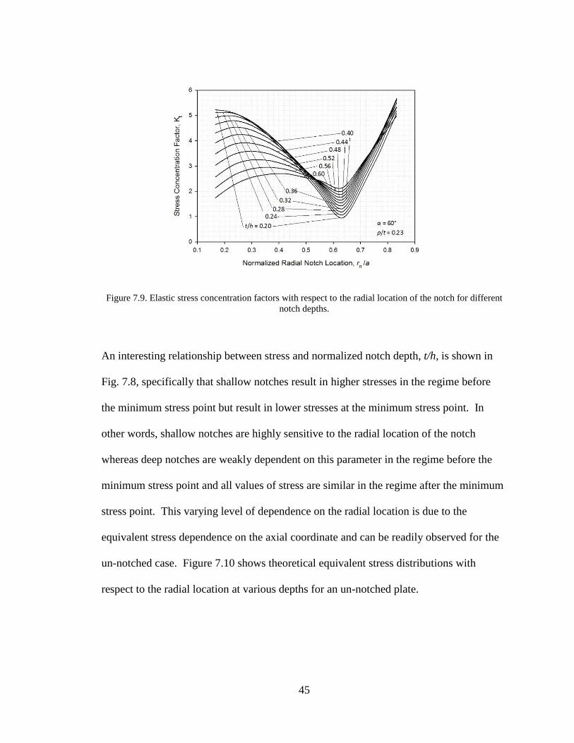
Figure 7.9. Elastic stress concentration factors with respect to the radial location of the

notch for different notch depths. ....................................................................................... 45

Figure 7.10. Theoretical equivalent stress distributions at various depths in an un-notched

plate. .................................................................................................................................. 46

ix

Figure 7.11. Theoretical equivalent stress distributions at various radial locations in an

un-notched plate. ............................................................................................................... 48

Figure 7.12. Elastic stress concentration factor, Kt, for various notch depths with other

parameters at benchmark values; (a) t/h = 0.20, (b) t/h = 0.30, (c) t/h = 0.40, (d) t/h =

0.50, (e) t/h = 0.60. ............................................................................................................ 51

Figure 7.13. Elastic stress concentration factors with respect to notch depth for different

notch angles. ..................................................................................................................... 52

Figure 7.14. Elastic stress concentration factors with respect to notch depth for different

notch root radii. ................................................................................................................. 52

Figure 7.15. Elastic stress concentration factor, Kt, for various notch root radii with other

parameters at benchmark values; (a) ρ/t = 0.13, (b) ρ/t = 0.18, (c) ρ/t = 0.23, (d) ρ/t =

0.28, (e) ρ/t = 0.33. ............................................................................................................ 55

Figure 7.16. Elastic stress concentration factors with respect to notch root radius for

different notch angles. ....................................................................................................... 56

Figure 7.17. Elastic stress concentration factors with respect to notch root radius for

different radial notch locations. ........................................................................................ 57

Figure 7.18. Elastic stress concentration factors with respect to notch root radius for

different notch depths. ...................................................................................................... 57

Figure 7.19. Elastic stress concentration factor, Kt, for various notch angles with other

parameters at benchmark values; (a) α = 45°, (b) α = 55°, (c) α = 65°, (d) α = 75°, (e) α =

85°. .................................................................................................................................... 60

x

Figure 7.20. Elastic stress concentration factors with respect to notch angle for different

notch depths. ..................................................................................................................... 61

Figure 7.21. Elastic stress concentration factors with respect to notch angle for different

notch root radii. ................................................................................................................. 62

Figure 7.22. Angular stress distribution parameter β along the root radius of the notch. 63

Figure 7.23. Angular stress distributions of Kt along the root radius of the notch for

various radial notch locations. .......................................................................................... 64

Figure 7.24. Angular stress distributions along the root radius of the notch for various

notch depths. ..................................................................................................................... 65

Figure 7.25. Angular stress distributions along the root radius of the notch for various

notch radii. ........................................................................................................................ 66

Figure 7.26. Angular stress distributions along the root radius of the notch for various

notch angles. ..................................................................................................................... 67

Figure 7.27. Vertical stress distribution parameter z. ...................................................... 67

Figure 7.28. Stress distributions ahead of the notch for various radial notch locations. . 68

Figure 7.29. Stress distributions ahead of the notch for various notch angles................. 69

Figure 7.30. Stress distributions ahead of the notch for various notch root radii. ........... 70

Figure 7.31. Stress distributions ahead of the notch for various notch angles................. 70

Figure 7.32. Mesh of benchmark notch configuration at refinement (a) level 1, (b) level

2, (c) level 3, and (d) level 4. ............................................................................................ 72

Figure 7.33. Angular stress distribution solutions for various mesh refinement levels. .. 73

xi

Figure B.1. Side view of fracture surfaces of smooth specimens from tensile experiments

at (a) 0.5 mm/s, (b) 0.05 mm/s, and (c) 0.005 mm/s. ........................................................ 93

Figure B.2. Isometric view of fracture surfaces of smooth specimens from tensile

experiments at (a) 0.5 mm/s, (b) 0.05 mm/s, and (c) 0.005 mm/s. ................................... 93

Figure B.3. SEM fractograph of smooth specimen from tensile test at 0.5 mm/s. .......... 93

Figure B.4. Side view of fracture surfaces of blunt notched specimens from tensile

experiments at (a) 0.5 mm/s, (b) 0.05 mm/s, and (c) 0.005 mm/s. ................................... 94

Figure B.5. Isometric view of fracture surfaces of blunt notched specimen from tensile

experiments at (a) 0.5 mm/s, (b) 0.05 mm/s, and (c) 0.005 mm/s. ................................... 94

Figure B.6. SEM fractographs showing smooth ridge of blunt notched specimen tested at

0.5 mm/s. ........................................................................................................................... 94

Figure B.7. SEM fractographs showing crack initiation of blunt notched specimen tested

at 0.5 mm/s. ....................................................................................................................... 95

Figure B.8. SEM fractographs showing smooth ridge of blunt notched specimen tested at

0.05 mm/s. ......................................................................................................................... 95

Figure B.9. SEM fractographs showing crack initiation of blunt notched specimen tested

at 0.05 mm/s. ..................................................................................................................... 95

Figure B.10. SEM fractographs showing smooth ridge of blunt notched specimen tested

at 0.005 mm/s. ................................................................................................................... 96

Figure B.11. SEM fractographs showing crack initiation of blunt notched specimen

tested at 0.005 mm/s. ........................................................................................................ 96

xii

Figure B.12. Side view of fracture surfaces of sharp notched specimens from tensile

experiments at (a) 0.5 mm/s and (b) 0.05 mm/s. .............................................................. 96

Figure B.13. Isometric view of fracture surfaces of sharp notched specimens from tensile

experiments at (a) 0.5 mm/s and (b) 0.05 mm/s. .............................................................. 97

Figure B.14. SEM fractographs showing smooth ridge of sharp notched specimen tested

at 0.5 mm/s. ....................................................................................................................... 97

Figure B.15. SEM fractographs showing crack initiation of sharp notched specimen

tested at 0.5 mm/s. ............................................................................................................ 97

Figure B.16. SEM fractographs showing smooth ridge of sharp notched specimen tested

at 0.05 mm/s. ..................................................................................................................... 98

Figure B.17. SEM fractographs showing crack initiation of sharp notched specimen

tested at 0.05 mm/s. .......................................................................................................... 98

xiii

List of Tables

Table 3.1. Various properties of Ultem 1000 (SABIC Innovative Plastics). ................... 18

Table 5.1 Summary of mechanical properties from the notched and un-notched tensile

tests. .................................................................................................................................. 22

Table 5.2 Average smooth circumferential band thicknesses for different strain rates. ... 27

Table 6.1. Ranges and increments of geometric v-notch parameters simulated. ............. 30

xiv

Nomenclature

α Notch angle

β Angular location along notch radius

εf, εy Elongation for fracture and yield respectively

θ Angular coordinate in circular plate

ν Poisson’s ratio

ρ Notch root radius

σθθ, σeqv, σrr, Hoop, equivalent, and radial stresses, respectively

σuc, σuf, σus, σut, Compressive, flexural, shear, and tensile strength, respectively

σoy, σy 0.2% offset yield strength and proportional limit, respectively

τrθ, τmax In-plane shear stress and maximum shear stress, respectively

a Radius of plate

d Distance between bottom of plate and tip of v-notch

Ec, Ef, Et, Compressive, flexural, and tensile modulus, respectively

h Thickness of plate

Kt Elastic or theoretical equivalent stress concentration factor

xv

KtE Elastic or theoretical stress concentration factor for shallow ellipse

KtH Elastic or theoretical stress concentration factor for hyperbolic

notch

Kts Elastic or theoretical shear stress concentration factor

l Semiaxis of ellipse

q0 Uniformly applied pressure

r Radial coordinate of circular plate

rn Notch radial location

t Notch depth

z Axial coordinate of circular plate

1

1. Introduction

In the aerospace and defense industries circular plates must be designed to either

withstand extreme pressure without fracture or in the case of guided projectiles, fracture

in a predictable manner under a specified load. Such a projectile is illustrated in Fig. 1.1.

In the case of guided projectiles, a stress raiser is incorporated into the component so that

the component will fracture under a specified load and along a desired path. The key

microstructural mechanism that confers fracturability is a ductile tearing mode. In most

cases, the stress concentration takes the form of a v-shaped notch (i.e., v-notch).

Although the geometric dependence of the stress concentration factor (SCF) for the v-

notch has been established for uniaxially loaded components (Appl and Koerner, 1969;

Noda and Takase, 1999) and components under bending (Leven and Frocht, 1953), the

case of the axisymmetrically loaded v-notched plate has yet to be studied. As such, the

main motivation behind the current study is to make up for the short comings in this field

of study.

To quantify the relationships between notch geometry and the resulting SCFs

along the notch root and ahead of the notch, parametric FEA was employed to facilitate

the simulation of over ten thousand geometric notch combinations. The state of localized

stress in the vicinity of the notch root determined from these simulations was

characterized for a wide range of notch geometries. SCFs Kt and Kts were defined which

denote the localized increase in equivalent and shear stress due to the presence of the

notch, respectively. The relationships between the magnitudes of these SCFs and notch

geometry were quantified resulting in mathematical models which provide the SCF for

2

any geometric notch combination within the studied ranges. Typical SCF behavior was

observed with respect to the radius of the notch root, ρ, i.e., notch root radius and the SCF

are inversely proportional. It was determined that within the range studied, the notch

angle α did not significantly affect the state of stress along the notch root. Similar

observations have been made for thin, v-notched beam elements in bending (Leven and

Frocht, 1953). With respect to the notch depth, t, it was observed that notches far from

mid-plane of the plate (i.e., shallow notches) produced higher SCFs than those close to

the mid-plane (i.e., as t/h approaches 0.5). This result is typical for plates in bending

because the flexural stresses within a plate are largest at the plate surfaces and decrease to

a minimum at the neutral axis (i.e., mid-plane). More novel observations were made with

respect to the radial location of the notch rn, due to the unique stress state within an

axisymmetrically loaded clamped circular plate. It was determined that the radial

location of the notch had the greatest influence over not only the magnitude of the SCF,

but the stress distributions along the notch root and ahead of the notch. Analytical

solutions of the stress state throughout an un-notched plate based on elastic theory were

used as constitutive models to predict SCF relationships with respect to the radial

coordinate for notched plates. Numerous SCF figures were developed which illustrate

SCF trends with respect to individual geometric notch parameters. Finite element

analysis stress contours are shown for a wide range of notch geometries which depict not

only the localized increase in stress, but the relative vicinity within the plate of which the

stress concentration is realized. This stress concentration sphere of influence was

quantified by comparing stress distributions within notched plates and equivalent un-

notched plates.

3

Figure 1.1. Guided projectile utilizing notched circular plate component.

The contents of this thesis continue with a thorough discussion of axisymmetric

plate bodies and other background material (Chapter 2). The Ultem 1000 material is

discussed in Chapter 3 including material properties, uses throughout various industries,

and relevant research findings pertaining to the fracture behavior of Ultem 1000. This

section is followed by the experimental approach which details the experimental test

procedures employed (Chapter 4). Chapter 5 discusses the results obtained from the

experiments, both empirically and through fractography. Immediately following is a

discussion on numerical simulations (Chapter 6), which describes the FEM techniques

employed to derive relationships between notch geometry and the maximum stresses

within the vicinity of the notch. Within the results and discussion section (Chapter 7),

data obtained from the parametric FEA is analyzed and stress concentration factor trends

are presented along with stress distribution plots for numerous notch geometry

configurations. The thesis conclusions are presented in Chapter 8. Numerical

simulations, further mechanical testing, and other proposals for future work are reported

in Chapter 9. Codes developed throughout the study are found in Appendix A and

photographs documenting the fracture surfaces from the experiments are given in

Appendix B.

4

2. Literature Review

2.1 Application

Circular plate components are commonly used in industry applications such as

pressure vessel closures, guided projectiles, pump diaphragms, clutches, and turbine disks

(Reddy, 1999). The accurate prediction of the stress and strain response to various

loading conditions within circular plates is of particular importance to plate component

designers. In the majority of applications, circular plate components are designed to

withstand static pressure loads subject normal to the plate face without failing, but in

specialized cases such as guided projectiles, circular plates are designed to rupture under

a specified dynamic load, as shown in Fig. 2.1. Either fracturing prematurely or failing to

fracture under the specified load would result in mission failure. To ensure the plate

fractures along a desired path, a stress raiser in the form of a v-notch is designed on the

plate surface concentric to the plate axis, as shown in Fig. 2.2. The fracture surface of a

v-notched Ultem 1000 circular plate is shown in Fig. 2.3. The plate shown in Fig. 2.3 is

upside down from the orientation shown in Fig. 2.2.

Although exact solutions exist for the state of stress throughout smooth circular

plates (Reddy, 1999) and very accurate approximations have been formulated for stress

concentration factors resulting from v-notches for a variety of simple loading conditions

(Noda and Takase, 1999), the effects that v-notches have on circular plates under

axisymmetric loads have yet to be characterized in literature.

5

Figure 2.1. Schematic illustrating service loading condition of notched circular plates in guided projectiles.

Figure 2.2. V-notched circular plate.

Figure 2.3. Outer ring portion of Ultem 1000 circular plate after fracture along v-notch.

Ductile tears

along fracture

surface

V-notch face

e

Dynamic pressure

Fixed end cap

6

2.2 SCFs and V-Notches

It is often the case that a structural component will contain geometric

discontinuities that differentiate the local state of stress from the remote or nominal stress

field. Examples of notch shaped stress raisers include shaft shoulders, relief grooves,

spring retention grooves, reentrant corners, and notched fatigue test specimens (Pilkey,

1997). The elastic or theoretical stress concentration factor is defined as the ratio

between the maximum stress within this annulus local to the notch root to some reference

stress (i.e., nominal or remote for a material subjected to nominally elastic conditions).

The reference stress chosen depends on the type of stress raiser, component geometry,

and loading condition. A comprehensive collection of stress concentration factors for a

wide variety of structural components, stress raisers, and loading conditions can be found

in the literature (Pilkey, 1997). Stress concentration factor plots for v-notched members

in uniaxial tension (Appl and Koerner, 1969) and in bending (Levin and Frocht, 1953) are

shown in Fig. 2.3 and Fig. 2.4, respectively.

Classical formulations for theoretical stress concentration factors of deep

hyperbolic (KtH) and shallow elliptical notches (KtE) were proposed by Neuber and have

proven to provide accurate results for either deep or shallow notches (Neuber, 1958).

Also proposed by Neuber (1958) was a relation for the stress concentration factor of

notches with arbitrary shapes based on the stress concentration factors of the shallow

elliptical and deep hyperbolic notches:

𝐾𝑡𝑛 = 1 + (𝐾𝑡𝐸 − 1)2(𝐾𝑡𝐻 − 1)2

(𝐾𝑡𝐸 − 1)2 + (𝐾𝑡𝐻 − 1)2 (2.1)

7

Here, KtE and KtH are the stress concentration factors of notches with the same

geometric notch parameters of the notch under consideration. A set of formulae

providing stress concentration factors accurate within 1% for any shape v-notch in a

cylindrical test specimen subject to various loading conditions was proposed by Noda and

Takase based on numerical results (Noda and Takase, 1999).

Figure 2.3. Stress concentration factors for a flat tension bar with opposite v-shaped notches.

8

Figure 2.4. Stress concentration factors for a thin beam element in bending with a v-shaped notch.

2.3 Theory of Elasticity for Axisymmetric Plates under Bending

An analytical approach based on the theory of elasticity has been used to

determine the state of stress and deformation behavior at any point within a circular plate

under a variety of loading conditions and boundary conditions. The general solution for

the deflection and stress state was defined by Reddy (1999) for a thin circular clamped

plate under a uniformly distributed load, as shown in Fig. 2.5. A circular plate is

classified as thin if the thickness does not exceed one-tenth of the diameter. This

comparatively small thickness allows for 2D equations to accurately characterize the

stresses throughout the plate (e.g. σzz = 0). These relations were formulated from the

classical elastic Kirchhoff assumptions that lines normal to the mid plane prior to bending

remain normal, straight, and in-extensible.

9

Figure 2.5. Circumferentially clamped plate subject to axisymmetric pressure distribution; (a) cross

sectional view, (b) top view (Reddy, 1999).

The derivation of such relations in polar coordinates begins with the general

equations for a circular plate subject to an arbitrarily distributed transverse load q(r)

applied to the top surface and temperature distribution ΔT(r, z), i.e.,

𝐷𝑤0 𝑟 = 𝐻 𝑟 + 𝑐2

𝑟2

4+ 𝑐4 (2.2)

𝐷

𝑑𝑤0

𝑑𝑟= 𝐻′ + 𝑐2

𝑟

2 (2.3)

𝑀𝑟𝑟 = − 𝐻′′ +

𝜈

𝑟𝐻′ −

1 + 𝜈

2𝑐2 (2.4)

𝑀𝜃𝜃 = − 𝜈𝐻′′ +

1

𝑟𝐻′ −

1 + 𝜈

2𝑐2 (2.5)

𝜎𝑟𝑟 = −

12𝑧

ℎ3 𝐻′′ +𝜈

𝑟𝐻′ +

1 + 𝜈

2𝑐2 (2.6)

𝜎𝜃𝜃 = −

12𝑧

ℎ3 𝜈𝐻′′ +1

𝑟𝐻′ +

1 + 𝜈

2𝑐2 (2.7)

Here, w0 is the plate deflection and Mrr, σrr, Mθθ, and σθθ, are the radial and tangential

components of the bending moments and stresses, respectively. In the above equations, r

(a) (b)

10

is the radial coordinate of the plate, z is the axial coordinate of the plate, ν is the Poisson’s

ratio, c2 and c4 are constants determined from boundary conditions, and D is the flexural

rigidity of the plate which is expressed

𝐷 =

𝐸ℎ3

12 1 − 𝑣2 (2.8)

where h is the thickness of the plate and E is the modulus of elasticity (Timoshenko,

1961; Wang, 2004). The function H is defined

𝐻 = 𝐹 − 𝐺 (2.9)

where functions F and G are written

𝐹(𝑟) =

1

𝑟 𝑟

1

𝑟 𝑟 𝑞 𝑟 𝑑𝑟𝑑𝑟𝑑𝑟𝑑𝑟 (2.10)

𝐺(𝑟) =

1

(1 − 𝜈)

1

𝑟 𝑟𝑀𝑇𝑑𝑟𝑑𝑟 (2.11)

and the thermal moment MT is expressed

𝑀𝑇 = 𝐸𝛼 Δ𝑇

ℎ2

−ℎ2

𝑟, 𝑧 𝑧𝑑𝑧 (2.12)

Here, α is the coefficient of thermal expansion and ΔT is the temperature gradient. For

the case of circumferentially clamped plates subjected to an isothermal axisymmetric

pressure, the boundary conditions require fixed conditions at the circumference of the

plate (i.e., w0 = 0 and 𝑑𝑤0 𝑑𝑟 = 0 at r = a). From these boundary conditions and from

Eqs. 2.2 and 2.3, the constants c2 and c4 can be solved for and are expressed

𝑐2 = −

𝑞0𝑎2

8, 𝑐4 =

𝑞0𝑎2

64 (2.13)

11

where q0 is the uniformly distributed load and a is the radius of the plate. From Eqn. 2.2,

the deflection of the midsection of the plate as a function of radius is given as

𝑤0 𝑟 =

𝑞0𝑎4

64𝐷 1 −

𝑟2

𝑎2

2

(2.14)

The maximum deflection is found at the center of the plate, i.e,

𝑤𝑚𝑎𝑥 =

𝑞0𝑎4

64𝐷 (2.15)

The bending moments are a function of the radial coordinate only and from Eqs. 2.4 and

2.5 are expressed as

𝑀𝑟𝑟 𝑟 =

𝑞0𝑎2

16 1 + 𝑣 − 3 + 𝑣

𝑟2

𝑎2

(2.16)

𝑀𝜃𝜃 𝑟 =

𝑞0𝑎2

16 1 + 𝑣 − 1 + 3𝑣

𝑟2

𝑎2 (2.17)

The maximum magnitude of the moments are realized at the circumferential edge and are

expressed

𝑀𝑟𝑟 𝑎 = −

𝑞0𝑎2

8

(2.18)

𝑀𝜃𝜃 𝑎 = −

𝜈𝑞0𝑎2

8 (2.19)

The out of plane bending moment Mrr and the in plane bending moment Mθθ are shown

graphically as a function of the radial coordinate in Fig. 2.6.

12

Figure 2.6. In-plane and out-of-plane bending moments throughout circular plate.

From the solution of Eqs. 2.6 and 2.7, the radial stress σrr and the tangential stress σθθ can

be expressed in polar coordinates, i.e.,

𝜎𝑟𝑟 𝑟, 𝑧 =

3𝑞0𝑎2𝑧

4ℎ3 1 + 𝑣 − 3 + 𝑣

𝑟2

𝑎2 (2.20)

and

𝜎𝜃𝜃 𝑟, 𝑧 =

3𝑞0𝑎2𝑧

4ℎ3 1 + 𝑣 − 1 + 3𝑣

𝑟2

𝑎2 (2.21)

Similar to simple beam problems, the flexural stresses are zero at the neutral axis (z = 0);

however, unlike typical beam problems, the stress distribution elsewhere is a function of

material properties. The radial and tangential components of stress are illustrated on a

differential element in Fig 2.7.

13

Figure 2.7. Radial and tangential components of stress on a differential element of circular plate.

The maximum stress is found at the clamped boundary on the top surface of the plate and

is given

𝜎𝑟𝑟 𝑎, −

ℎ

2 = −

6𝑀𝑟𝑟 (𝑎)

ℎ2=

3𝑞0

4 𝑎

ℎ

2

(2.22)

Under plane stress conditions, from Eqs. 2.20 and 2.21, the effective stress throughout the

plate can be obtained, i.e.,

𝜎𝑒𝑞𝑣 =

1

2 𝜎𝑟𝑟 − 𝜎𝜃𝜃 2 + 𝜎𝑟𝑟

2 + 𝜎𝜃𝜃 2 (2.23)

The radial, tangential, and equivalent stresses as a function of the radial coordinate are

shown in Fig. 2.8 for a normalized axial location z/h = -0.20. The theoretical stresses at

this particular plate depth are shown because this depth corresponds to the benchmark v-

14

notch depth chosen for this study and a comparison of the stresses between the

benchmark smooth plate and the benchmark notched will be discussed in Chapter 6.

Solutions to a variety of cases with various boundary conditions and load states

derived from Kirchhoff plate theory can be found in the literature (Szilard, 1974; Ugural,

1999; Reddy, 1999). More specifically, the boundary conditions which have been

previously investigated include simply supported edges, clamped edges, and elastic

foundations. Additionally, plates subject to uniform and non-uniform pressure

distributions as well as point loads and thermal loads have been studied.

Figure 2.8. Radial, tangential, and equivalent stresses at an axial location z/h equal to -0.20.

15

3. Materials

Polyetherimide, also referred to as Ultem, is a widely-used amorphous

thermoplastic with applications ranging from the aerospace to medical industries. Ultem

is extensively used in the aerospace and defense industries due to its high strength, heat

resistance, and relatively low-weight compared to aluminum alloys. The mechanical,

physical, and thermal properties of Ultem, shown in Table 1, allow for such versatility in

a wide variety of industry applications. For example, Ultem was used to injection mold a

variety of interior and structural components in the Fokker 50 and 100 series aircraft

(Savage, 1988). Also, because of the remarkable resistance to corrosive cleaning

chemicals and thermal cycling it displays, Ultem was chosen for sterilization trays and

surgical probes that withstand daily autoclaving (Johnson, 1998).

The mechanical properties of Ultem and similar plastics at various temperatures

and strain rates have been extensively studied by various researchers. It was found that,

generally, an increase in strain rate corresponds to an increase in tensile strength among

Ultem and similar thermoplastics (Schobig et al., 2008). Similar results were reported by

Bordonaro and Krempl (1993) when cylindrical plastic specimens were tensile tested at

various strain rates, ranging from 10-3

to 10-6

s-1

. The temperature effects on the stress-

strain relationships of Ultem were studied by Pecht and Wu (1994). They observed that

increases in temperature cause a decrease in the yield strength and modulus of elasticity

of Ultem while an increase in strain rate causes an increase in tensile strength. These

observations are depicted graphically in Fig. 3.1. Pecht and Wu (1994) also investigated

temperature effects on two other polymers, Kapton and SE45, and found that the lower

16

glass transition temperature of Ultem can be attributed to the ether and imide linkages

present in Ultem. The chemical structure of Ultem 1000 can be found in Fig. 3.2 (Pecht

and Wu, 1994).

Figure 3.1. Stress-strain curves corresponding to Ultem tensile tests under various temperatures and strain

rates (Pecht and Wu, 1994).

Figure 3.2. Chemical composition of Ultem 1000 (Pecht and Wu, 1994).

The fracture behavior of Ultem has been studied under a wide range of

temperatures by Kim and Ye (2004). They employed mechanical tests on compact

tension (CT) specimens of various thicknesses at a crosshead speed of 2 mm/min subject

17

to various temperatures (24°C, 80°C, 130°C) to determine the relationship between

temperature and plane strain fracture toughness. They observed three different crack

propagation modes, namely unstable, stable and mixed, depending on the temperature

and specimen thickness. It was found that at room temperature, all the specimens

exhibited brittle fracture and ductile fracture was observed in specimens at higher

temperatures. These results are shown in Fig. 3.3.

Figure 3.3. Load displacement curves for Ultem CT specimens of various thicknesses (6, 12, and 22 mm)

and various temperatures (Kim and Ye, 2004).

Other standard mechanical, thermal, and electrical properties of Ultem have been

well characterized and can be found in the literature along with many experiments

concerning fatigue, creep, and wear behaviors (Stokes, 1988; Bijwe et al., 1991; Tou and

Zihui, 2007; Facca et al., 2007; Smmazcelik, 2008). A variety of Ultem grades are

available from SABIC Innovative Plastics which encompass a large range of mechanical,

thermal, and chemical properties. For example, Ultem grades are available with glass

18

fiber or PTFE fillings of up to 45% which increases strength and enhances flow

properties. A number of other enhancements are available such as transparency

characteristics and finish properties which allow for safe use in the medical and food

handling industries. The specific grade of resin chosen for the present study is Ultem

1000 which is unfilled, transparent, and exhibits standard flow characteristics.

Table 3.1. Various properties of Ultem 1000 (SABIC Innovative Plastics).

Mechanical Properties Value (English) Value (SI)

Tensile Modulus, Et 475 ksi 3.28 GPa

Compressive Modulus, Ec 480 ksi 3.31 GPa

Flexural Modulus, Ef 500 ksi 3.45 GPa

Poisson’s Ratio, ν 0.36 -

Elongation (Yield), εy 7.0 % -

Tensile Strength, σut 16.5 ksi 113.8 MPa

Compressive Strength, σuc 22 ksi 151.7 MPa

Shear Strength, σsu 15 ksi 103.4 MPa

Flexural Strength, σuf 20 ksi 137.9 MPa

Elongation (Fracture), εf 60 % -

Izod Impact Strength, Notched 1.0 ft-lbs/in 0.034 J/m

Rockwell Hardness 109 (“M” Scale) -

Physical Properties Value (English) Value (SI)

Specific Gravity 1.28 -

Thermal Properties Value (English) Value (SI)

CLTE - Flow, αf 0.000031 in/in/°F -

CLTE - Tansverse, αt 0.000030 in/in/°F -

19

4. Experimental Approach

Uniaxial tensile tests were employed on smooth Ultem 1000 cylindrical coupons

to determine the tensile properties of Ultem 1000 at room temperature and to investigate

the failure behavior of Ultem 1000 under uniaxial tension. Experiments were also

conducted on two sets of cylindrical notched specimens with different notch root radii to

determine the effects of v-notch stress concentrations on the strength and fracture

properties of Ultem 1000. The root radii for the v-notched specimens were 0.035 (ρ/t =

0.23) and 0.016 (ρ/t = 0.11) inches, respectively. The test coupons were machined from

extruded Ultem 1000 rod stock with a diameter of 0.5 inches. Tensile tests were

conducted until rupture at three cross head displacement rates, 0.5 mm/s, 0.05 mm/s, and

0.005 mm/s to characterize any mechanical property rate dependency. An MTS 100 kN

servohydraulic testing frame was used along with an MTS 632-53E-14 extensometer to

conduct the experiments and collect strain data, respectively. The three specimen

configurations used and the extensometer experimental setup are shown in Fig. 4.1 and

Fig. 4.2, respectively. The specimen conditioning and experimental procedure were

carried out in accordance with ASTM D638-08, under normal laboratory conditions with

an ambient temperature of 74°F and 50% humidity. The standard calls for at least five

tests to be conducted for each experimental configuration, but due to available resources,

only one experiment was performed per specimen type and strain rate.

The fracture surfaces of the tensile test specimens were examined using a Hitachi

S-3500N scanning electron microscope (SEM) to gain insight into the microstructural

mechanics facilitating fracture. Due to the non-conductivity of Ultem 1000, the fracture

20

surfaces were sputter coated with platinum to prevent a built up of static charge on the

fracture surface and to increase the signal resolution.

Figure 4.1. Tensile specimen configurations used.

Figure 4.2. Extensometer application.

Sharp notch Blunt notch

21

5. Experimental Results

Mechanical properties of Ultem 1000 under uniaxial tension such as the modulus

of elasticity, E, the ultimate tensile strength, σut, the fracture strain, εf, and the 0.2% offset

yield strength, σoy, were determined from the stress-strain curves of the un-notched

specimens. These values were also calculated for both notched cases; however, it should

be noted that the values between the notched and un-notched cases cannot be directly

compared and that the data for the notched cases is given for the sake of establishing a

complete record. Table 5.1 summarizes the data determined from the tensile tests of the

un-notched and notched specimens. The values of the modulus of elasticity and the

ultimate tensile strength from the smooth specimen experiments match closely to those

previously published (See Table 3.1). A rate dependency of the ultimate strength and the

yield strength for the smooth case is observed from the stress-strain diagram, as shown in

Fig. 5.1, where the ultimate and yield strength increase with strain rate. The observation

of an increase in yield strength with an increase in strain rate is consistent with the Eyring

theory of yield (Swallowe, 1999), described by the following relation:

𝜎𝑦 = 𝜎0 +

𝑅𝑇

𝜈log

2𝜀

𝜀 0 (5.1)

Here, σy is the yield stress, 𝜀 is the strain rate, T is the temperature, and 𝜀 0, ν, σ0, and R are

regression constants. The relationship between strain rate and the ultimate tensile

strength has been observed previously by Krempl (1993) for Ultem 1000 and other

thermoplastics. These results suggest that a high strain rate facilitates a more brittle

material response than a low strain rate for un-notched tensile experiments.

22

Table 5.1 Summary of mechanical properties from the notched and un-notched tensile tests.

Rate

(mm/s)

E

(GPa)

εf

(mm/mm)

σf (UTS)

(MPa)

Pmax

(N)

σy (0.2%)

(MPa

Un-notched

0.5 3.51 0.0510 111.5 3535 65.4

0.05 3.22 0.0583 110.0 3487 64.0

0.005 3.57 0.0541 104.0 3297 58.7

Blunt Notch (Kt = 2.0)

0.5 5.74 0.0193 101.9 3230 N/A

0.05 5.54 0.0245 119.6 3791 108.9

0.005 5.17 0.0253 113.0 3582 98.3

Sharp Notch (Kt = 3.0)

0.5 5.10 0.0219 105.2 3335 N/A

0.05 5.61 0.0199 99.3 3148 N/A

Figure 5.1. Engineering stress-strain curve for smooth specimens.

23

These trends are based on data from only a single experiment at each configuration and

therefore can be easily skewed by experimental error such as machining defects in the

test specimens.

The experimental results from the notched tensile tests provide insight into the

effects of a stress concentration on the fracture behavior of uniaxially loaded Ultem 1000.

In general, the presence of a v-notch facilitated brittle fracture behavior, which is

evidenced by the lack of a yield region on a force-strain diagram for the notched cases, as

shown in Fig. 5.2.

Figure 5.2. Force-strain diagram comparing smooth and notched specimens for tensile experiment at 0.05

mm/s.

The theoretical stress concentration factors for the notches used in these tensile

experiments were calculated from empirical relationships provided by Noda and Takase

(1999) which are functions of notch geometry and provide a Kt = 2.0 for ρ/t = 0.23 and Kt

= 3.0 for ρ/t = 0.11. From Fig. 5.2, it should be observed that higher stress concentration

24

factors facilitate fracture at lower strains than for lower stress concentration factors and

un-notched specimens. Another trend apparent in Fig. 5.2 is that the modulus of

elasticity increases with the stress concentration factor. An increase in the stiffness of a

material is often associated with brittle behavior and in this case could be a result of heat

imparted onto the material in the vicinity of the notch during machining.

In addition to an analysis of the stress-strain responses, fractography was

employed to explore the effects of strain rate and the presence of a v-notch on the fracture

behavior of uniaxially loaded Ultem 1000 specimens. Examination of the fracture

surfaces with optical microscopy and a SEM provides knowledge of the modes of

fracture present as well as the crack initiation location. For the smooth case, the effect of

strain rate on the failure mode, either ductile or brittle, is readily observed from the

fracture surfaces. A comparison between the relatively smooth fracture surfaces of a

specimen tested at 0.5 mm/s, shown in Fig. 5.3, and the rough fracture surface of a

specimen tested at 0.005 mm/s, shown in Fig. 5.4, illustrates the strain rate effect.

Detailed photographs of all the smooth tensile specimens tested, including side shots and

SEM photographs can be found in Appendix B.

25

Figure 5.3. Fracture surface of a smooth tensile specimen tested at 0.5 mm/s.

Figure 5.4. Fracture surface of a smooth tensile specimen tested at 0.005 mm/s.

For the notched cases, analysis of the fracture surfaces evidence brittle fracture

behavior, supporting the conclusions drawn from the force-strain curves for the notched

specimens. The fractography of the notched specimens focused on two areas of interest,

the assumed crack initiation point and smooth circumferential bands near the edges of the

specimen. The fracture initiation point was determined by tracing radial fracture

Crack initiation Fast fracture

Ductile tearing

26

propagation paths back to a location of relatively smooth surface. This smooth initiation

region is caused by relatively slow fracture speeds where adjacent fibers fracture all on

the same plane (Greenhalgh, 2009). From this point, the crack propagates radially with

increasing velocities, causing fracture to occur on multiple planes, which facilitates the

formation of a rough surface. The evolution of the surface topology is typically divided

into three distinct zones; the mirror, mist, and hackle (Greenhalgh, 2009). Figure 5.5

illustrates the crack initiation point, radial propagation lines, and these three zones.

Figure 5.5. SEM fractograph showing crack initiation of blunt notched specimen tested at 0.05 mm/s.

The thicknesses of the smooth circumferential bands observed in all of the notched

fracture surfaces were measured to determine if the thickness of the band was a function

of strain rate, and are summarized in Table 5.2. An example of these bands is shown on

the fracture surface of a blunt notched specimen tested at 0.005 mm/s, depicted in Fig.

5.6. From the data in Table 5.1, it appears that the thickness of the bands increase with

Mirror

Mist Hackle

Crack initiation

27

decreasing strain rate for the blunt notched specimen; however, this trend could be an

artifact of the few data points recorded.

Table 5.2 Average smooth circumferential band thicknesses for different strain rates.

Displacement rate

(mm/s)

Band thickness

(μm)

Blunt Notch (Kt = 2.0)

0.5 250

0.05 330

0.005 400

Sharp Notch (Kt = 3.0)

0.5 400

0.05 200

Figure 5.6. SEM fractograph showing smooth band of blunt notched specimen tested at 0.005 mm/s.

Multiple fractographs of each of the specimens tested, detailing the fracture surface and

circumferential bands are providing in Appendix B.

Smooth band

28

6. Numerical Simulation Approach

Because of the versatility and efficiency of such numerical methods, finite

element analysis was used to investigate the effects that notch geometry have on the

maximum stress on the surface and in the vicinity of a v-notch root on an

axisymmetrically loaded plate. Through the use of parametric codes, results from

thousands of combinations of notch geometries can be used to formulate numerical

relationships not feasible with traditional mechanical testing or elastic theory. The

ANSYS general-purpose software was used to numerically simulate the stress, strain, and

displacement fields of the component.

Taking advantage of the axisymmetric geometry of the model, only a 2D cross

section was required to accurately simulate the component, as shown in Fig. 6.1.

Boundary conditions restricting displacement in the radial and axial directions were

placed on the circumferential boundary of the plate. The appropriate displacement

boundary conditions are automatically imposed by ANSYS on the axial edge of the

model in an axisymmetric simulation. The top surface of the plate was subjected to a

uniformly distributed static pressure, q0. As shown in Fig. 6.1, no portion of the

distributed load was applied to the notch faces or root; however, cases where a fraction of

q0 are carried across the notch would reflect the service conditions more accurately, but is

saved for future research.

29

Figure 6.1. Automatic mesh and refinement in vicinity of notch for benchmark geometry.

An ANSYS input file, provided in Appendix A, was developed to facilitate

versatile parametric runs with highly customizable user control. The geometry of the

plate component was parametrically related to the dimensions and location of the notch.

The range and increments of specific variables could be easily manipulated for a variety

of custom parametric simulations. The normalized ranges of the geometric notch

parameters were chosen to encompass the broadest feasible range of geometric

combinations within the limits set by typical component machining and accurate FEA

solutions. More specifically, very sharp notch radii (ρ/t ≤ 0.20) were not considered

because such notches would be difficult and expensive to machine and the accuracy of

the FEA solutions for very sharp discontinuities are decreased. The geometric notch

parameter ranges and corresponding increments are given in Table 6.1.

30

Table 6.1. Ranges and increments of geometric v-notch parameters simulated.

rn/a t/h ρ/t α

0.17 0.20 0.13 40°

0.24 0.24 0.15 45°

0.30 0.28 0.17 50°

0.37 0.32 0.19 55°

0.43 0.36 0.21 60°

0.50 0.40 0.23 65°

0.57 0.44 0.25 70°

0.63 0.48 0.27 75°

0.70 0.52 0.29 80°

0.76 0.56 0.31 85°

0.83 0.60 0.33 90°

Limiting cases such as

rn/a → 0, rn/a → 1.0, t/h → 1.0, ρ/t → 0, α → 0°, (6.1)

and so on were left for future study. The one exception was that the smooth case was

investigated (i.e., rn/a is undefined, t = 0, and ρ is undefined). The plate radius, a, and

thickness, h, were held constant for all simulations. The benchmark notch geometry

consists of the following normalized parameters:

rn/a = 0.33, t/h = 0.20, ρ/t = 0.23, α = 60° (6.2)

31

The characterizing geometric parameters of the v-notch and circular plate are shown in

Fig. 6.2.

Figure 6.2. Characterizing geometric parameters for v-notched plate.

The FEA model is meshed entirely with PLANE82 8-noded quadrilateral

elements. This element was chosen for its ability to tolerate irregular shapes in automatic

meshes without much loss in accuracy. The ANSYS automatic meshing algorithm was

employed in the parametric simulations for efficient mesh adaptation to the varying notch

dimensions. Finite element modeling meshes for some of the extreme geometric

combinations such as a shallow notch, deep notch, and sharp notch are shown in Figs. 6.3

- 6.4. Automatic mesh refinement in the vicinity of the notch was utilized which reduced

the area of the elements at the notch tip by approximately a factor of two thousand from

those in remote regions of the plate. The ratio of the average notch tip element side

length to the benchmark normalized notch tip radius ρ/t is 0.0048. Mesh refinement,

illustrated in Fig. 6.1, consisted of element cleaning and smoothing in addition to size

reduction. The average number of elements and nodes utilized in the parametric runs

32

were 2,700 and 8,400 respectively. The component is subjected to quasi-static loading

and the materials assumed to behave elastically (See Table 3.1). To ensure that the

results can be compared with future elastic-plastic studies, q0 is designed to impart states

of stress that do not exceed the yield strength of Ultem 1000.

Figure 6.3. Automatic mesh generated for a shallow notch (t/h = 0.20) with otherwise benchmark

parameters.

Not refined Moderately refined

Highly refined

33

Figure 6.4. Automatic mesh generated for deep notch (t/h = 0.60) with otherwise benchmark parameters.

Figure 6.5. Automatic mesh generated for sharp notch (ρ/t = 0.20) with otherwise benchmark parameters.

34

7. Results and Discussion

The discussion of the numerical simulation results are divided into an analysis of

elastic stress concentration factors with respect to notch geometry and an investigation of

the effects notch geometry has on stress distributions at the notch root. The former is

subdivided into individual detailed discussions for each geometric notch parameter

supplemented with stress concentration factor plots and curve fit equations. The stress

distribution portion of the discussion provides insights into the angular stress

distributions along the surface of the notch as well as vertical stress distributions ahead of

the notch supported by stress distribution plots and FEA images.

To verify the accuracy of the FEM, the un-notched plate was simulated and the

equivalent stresses σeqv and maximum shear stresses τmax were compared to those obtained

from analytical solutions and are shown graphically in Fig. 7.1 and 7.2, respectively.

Figure 7.1. Comparison between the equivalent stresses obtained from the FEA and analytical solutions.

35

Figure 7.2. Comparison between the max shear stresses obtained from the FEA and analytical solutions.

From these plots, it is shown that the results from the FEA match closely to those

obtained from the analytical solutions for the principal stresses; however, there is a

deviation between the analytical and numerical results of the equivalent stress. This is

due to the assumption made in the analytical solution that there are no stresses in the axial

direction This assumption, however, is not made in the FEA and axial stresses are

present in the finite element solution. These axial stresses contributed to the equivalent

stress value in the FEM and thereby result in a deviation from the analytical solution.

The stress concentration factor, Kt, is defined as the equivalent stress divided by

the maximum shear stress in an un-notched plate of equal geometry, i.e.,

𝐾𝑡 =

2𝜎𝑒𝑞𝑣 (𝑟, 𝑧)

𝜎𝑟𝑟(max )(𝑢𝑛 )

− 𝜎𝜃𝜃 (max )(𝑢𝑛 )

(7.1)

36

where σeqv(r,z) is the equivalent stress, and 𝜎𝑟𝑟 (max )(𝑢𝑛 )

and 𝜎𝜃𝜃(max)(𝑢𝑛)

are the analytically

derived maximum radial and hoop stresses, respectively, in an equivalent un-notched

plate. Substituting in the theoretical maximum stresses from Eqs. 2.20 and 2.21 for

𝜎𝑟𝑟 (max )(𝑢𝑛 )

and 𝜎𝜃𝜃(max)(𝑢𝑛)

in Eqn. 7.1 yields

𝐾𝑡 =

8𝜎𝑒𝑞𝑣 (𝑟, 𝑧)

3𝑞0 𝑎ℎ

2(1 − 𝜈)

(7.2)

The shear stress concentration factor Kts is defined as

𝐾𝑡𝑠 =

8𝜏𝑚𝑎𝑥 (𝑟, 𝑧)

3𝑞0 𝑎ℎ

2(1 − 𝜈)

(7.3)

Here τmax is the maximum shear stress determined from

𝜏𝑚𝑎𝑥 =𝜎1 − 𝜎3

2

(7.4)

where σ1 and σ3 are the maximum and minimum principal stresses, respectively.

Stress contours of the normalized equivalent stresses and the normalized

maximum shear stresses throughout the un-notched plate subject to axisymmetric

pressure are shown in Fig. 7.3. The stress contours appear similar between the equivalent

and max shear stress and differ only in magnitude. Stress contours illustrating the

equivalent stresses and maximum shear stresses for the benchmark notch geometry are

shown in Fig. 7.4. From this figure, the localized increase in stress due to the presence of

the notch is clearly shown and the maximum stress concentration factor of approximately

5.0 is found on the surface of the notch root.

37

Figure 7.3. Elastic stress concentration factors, Kt (a), and Kts (b), contours for un-notched plate.

(a)

Kt

(b)

Kts

38

Figure 7.4. Elastic stress concentration factors, Kt (a), and Kts (b), contours for benchmark notched

geometry.

Kt

Kts

(a)

(b)

39

The effect notch geometry has on these SCFs are illustrated in a number of stress

concentration factor diagrams. These plots were developed directly from data extracted

from the parametric FEM simulations. For ease of analysis, the diagrams are divided into

sections corresponding to the geometric parameter on the abscissa, namely rn/a, α, t/h, or

ρ/t. Each family of figures with the identical parameter on the abscissa consists of three

separate plots, one for each of the other parameters being simultaneously varied. In each

case, the two geometric notch parameters held constant take on benchmark conditions.

An important characteristic of stress concentration factors is the size of the zone

in which the effect of the stress raiser is realized. Knowledge of the size of this zone is

important because outside of this neighborhood of localized stress, the state of stress can

be easily determined by traditional analytical methods depending on the loading

condition and component geometry; therefore, only the stresses within this small zone

need to be explored. The most direct application of this knowledge is in the setup of the

FEM. The mesh outside of this zone is permitted to be coarse and only within the small

area of interest is significant mesh refinement needed. To establish the relative size of

the region of affected stress, the stress distribution along a horizontal line at a depth equal

to the benchmark notch depth in both the smooth and notched case are plotted on the

same diagram. Such a diagram is shown graphically in Fig. 7.5. Analysis of this

comparative figure reveals that the stress distributions between the notched and smooth

case differ significantly only in a zone equal to approximately 2.0% of the plate radius.

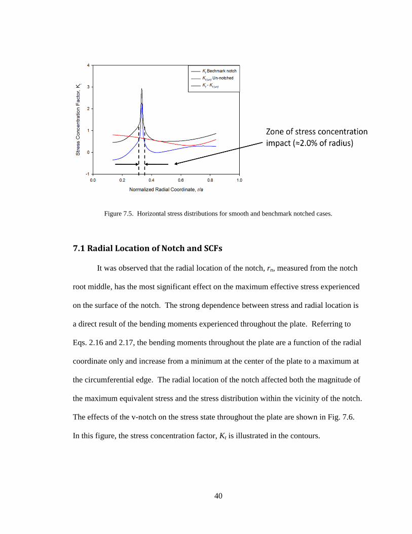
40

Figure 7.5. Horizontal stress distributions for smooth and benchmark notched cases.

7.1 Radial Location of Notch and SCFs

It was observed that the radial location of the notch, rn, measured from the notch

root middle, has the most significant effect on the maximum effective stress experienced

on the surface of the notch. The strong dependence between stress and radial location is

a direct result of the bending moments experienced throughout the plate. Referring to

Eqs. 2.16 and 2.17, the bending moments throughout the plate are a function of the radial

coordinate only and increase from a minimum at the center of the plate to a maximum at

the circumferential edge. The radial location of the notch affected both the magnitude of

the maximum equivalent stress and the stress distribution within the vicinity of the notch.

The effects of the v-notch on the stress state throughout the plate are shown in Fig. 7.6.

In this figure, the stress concentration factor, Kt is illustrated in the contours.

41

(a)

(b)

Kt

Kt

42

(c)

(d)

Kt

Kt

43

Figure 7.6. Elastic stress concentration factor, Kt, for various radial notch locations with other parameters

at benchmark values; (a) r/a = 0.17, (b) r/a = 0.33, (c) r/a = 0.50, (d) r/a = 0.67, (e) r/a = 0.83.

It is shown that sharp notch radii yield higher stress concentration factors than

blunt radii (Fig. 7.7) and smaller notch angles yield higher stress concentration factors

than larger ones (Fig 7.8). These trends are both intuitive and consistent with v-notch

elastic stress concentration factor results, and they have been observed in numerous stress

concentration factor experiments (Pilkey, 1997). It can be observed from Fig. 7.9 that the

stresses within the notch are not highly sensitive to the notch angle within the range

studied. Leven and Frocht (1953) found that for a v-notched, thin beam element in

bending that the notch angle did not affect the stress concentration factor for notch angles

between 0° and 90°.

(e)

Kt

44

Figure 7.7. Elastic stress concentration factors with respect to the radial location of the notch for different

notch root radii.

Figure 7.8. Elastic stress concentration factors with respect to the radial location of the notch for different

notch angles.

45

Figure 7.9. Elastic stress concentration factors with respect to the radial location of the notch for different

notch depths.

An interesting relationship between stress and normalized notch depth, t/h, is shown in

Fig. 7.8, specifically that shallow notches result in higher stresses in the regime before

the minimum stress point but result in lower stresses at the minimum stress point. In

other words, shallow notches are highly sensitive to the radial location of the notch

whereas deep notches are weakly dependent on this parameter in the regime before the

minimum stress point and all values of stress are similar in the regime after the minimum

stress point. This varying level of dependence on the radial location is due to the

equivalent stress dependence on the axial coordinate and can be readily observed for the

un-notched case. Figure 7.10 shows theoretical equivalent stress distributions with

respect to the radial location at various depths for an un-notched plate.

46

Figure 7.10. Theoretical equivalent stress distributions at various depths in an un-notched plate.

From these stress distributions it can be seen that for shallow depths within the plate, the

radial location strongly affects the stress magnitude, whereas for depths closer to the

neutral axis, this dependence on radial location becomes weak. A more detailed

discussion on the effect notch depth has on the maximum equivalent stress is provided in

the next chapter. A general trend observed in all three notched plate stress concentration

factor plots is similar to that of the un-notched case. Specifically, the equivalent stress

reaches a minimum point at approximately rn/a = 0.63. This location of minimum stress

can be derived mathematically for the un-notched case. The simplified equivalent stress

formula for plane stress in polar coordinates can be expressed as

𝜎𝑒𝑞𝑣 =1

2 𝜎𝑟𝑟 − 𝜎𝜃𝜃 2 + 𝜎𝑟𝑟

2 + 𝜎𝜃𝜃 2 (7.5)

Taking the derivative of this relation with respect to r and finding the positive root yields

the following expression

47

𝑟

𝑎=

(𝜈 + 1) 14𝜈2 + 4𝜈 + 14

7𝜈2 + 2𝜈 + 7

(7.6)

Equation 7.6 provides the radial location within an un-notched plate for which the von

Mises stress will be a minimum and states that this location is a function of Poisson’s

ratio only. Substituting the value of Poisson’s ratio for Ultem 1000 into Eqn. 7.6 yields a

normalized radial location of r/a = 0.65 which agrees well with results from the FEA.

Another trend similar between all the plots is that stress dependence on the second

parameter being varied (the one not on the abscissa) is significantly more pronounced

before this minimum stress point, whereas after this minimum point the stress is

dependent mostly on the radial location of the notch. This observation can be explained

by the relationship between the bending moments within the un-notched plate and the

radial location. As the radial location approaches the clamped circumferential edge, the

bending moments rise to their maximum, as is shown in Eqs. 2.18 and 2.19; therefore, the

stresses in this regime are dominated by the radial coordinate.

7.2 Notch Depth and SCFs

The maximum equivalent stress on the surface of the notch was found to be

significantly affected by the depth of the notch. It was found that shallow notches caused

higher stress concentration factors than deep notches. To understand the relationship

between notch depth and stress, first dependence of stress on the axial coordinate within

an un-notched plate is explored. Figure 7.11 represents vertical equivalent stress

distributions from the top of the plate to the mid-plate at various radial locations within

an un-notched plate.

48

Figure 7.11. Theoretical equivalent stress distributions at various radial locations in an un-notched plate.

In these figures, the normalized axial location, z/h, ranges from -0.5, which corresponds

to the top surface of the plate to 0.0, which corresponds to the mid-plane of the plate.

From this figure, it is evident that the magnitude of equivalent stress is the greatest at the

surface of the plate and decreases linearly to zero at the mid plane. A similar stress

dependence on the axial location is present in the notched case. Finite element analysis

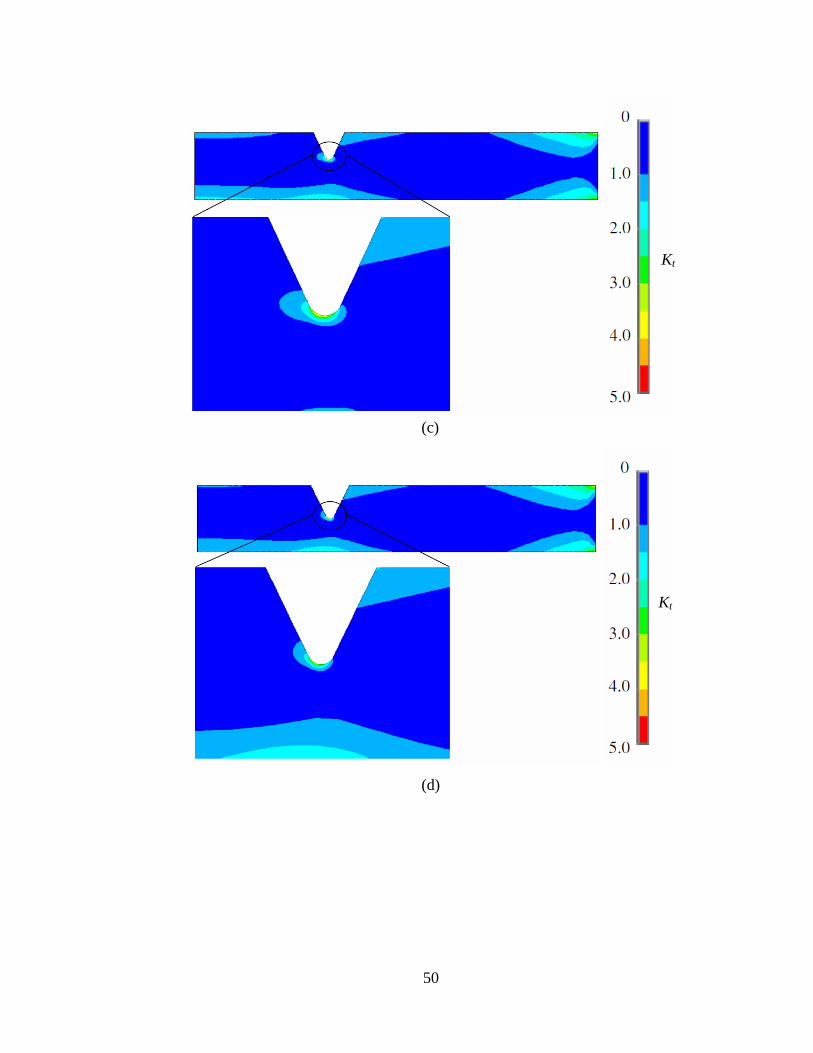
contours of the stress concentration factor, Kt, for plates with various notch depths are

shown in Fig. 7.12. It is readily observed from this figure that as the notch depth

approaches the mid-plane, the maximum stresses in the vicinity of the notch decrease.

Top Surface

Mid-plate

49

(a)

(b)

Kt

Kt

50

(c)

(d)

Kt

Kt

51

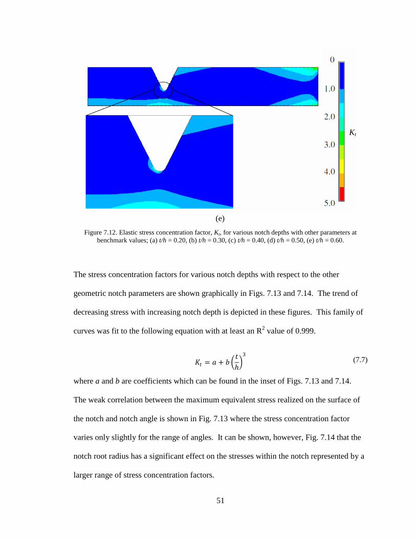
Figure 7.12. Elastic stress concentration factor, Kt, for various notch depths with other parameters at

benchmark values; (a) t/h = 0.20, (b) t/h = 0.30, (c) t/h = 0.40, (d) t/h = 0.50, (e) t/h = 0.60.

The stress concentration factors for various notch depths with respect to the other

geometric notch parameters are shown graphically in Figs. 7.13 and 7.14. The trend of

decreasing stress with increasing notch depth is depicted in these figures. This family of

curves was fit to the following equation with at least an R2 value of 0.999.

𝐾𝑡 = 𝑎 + 𝑏

𝑡

ℎ

3

(7.7)

where a and b are coefficients which can be found in the inset of Figs. 7.13 and 7.14.

The weak correlation between the maximum equivalent stress realized on the surface of

the notch and notch angle is shown in Fig. 7.13 where the stress concentration factor

varies only slightly for the range of angles. It can be shown, however, Fig. 7.14 that the

notch root radius has a significant effect on the stresses within the notch represented by a

larger range of stress concentration factors.

(e)

Kt

52

Figure 7.13. Elastic stress concentration factors with respect to notch depth for different notch angles.

Figure 7.14. Elastic stress concentration factors with respect to notch depth for different notch root radii.

𝐾𝑡 = 𝑎 + 𝑏 𝑡

ℎ

3

α a b

45° 4.7848 -8.5157

54° 4.7119 -9.1344

63° 4.6277 -9.8146

72° 4.5306 -10.5574

81° 4.4007 -11.1734

90° 4.2435 -11.8538

𝐾𝑡 = 𝑎 + 𝑏 𝑡

ℎ

3

ρ/h a b

0.040 6.0065 -13.0198

0.046 5.6317 -12.1070

0.052 5.3263 -11.3692

0.058 5.0680 -10.6595

0.064 4.8438 -10.0260

0.070 4.6594 -9.6328

0.076 4.4898 -9.1105

0.082 4.3405 -8.7450

0.088 4.2073 -8.3726

0.094 4.0887 -8.0481

0.100 3.9839 -7.7781

53

7.3 Notch Root Radius and SCFs

The relationship observed between the notch root radius and the maximum

stresses on the surface of the v-notch was consistent with typical notch problems. More

specifically, the stresses in the vicinity of the notch where shown to increase as the notch

root radius was decreased. This trend is illustrated in a number of stress contours, shown

in Fig. 7.15, representing the elastic stress concentration factor, Kt, for v-notches with

various root radii. From these contours, the larger stresses are apparent in the notches

with sharper notch radii

(a)

Kt

54

(b)

(c)

Kt

Kt

55

Figure 7.15. Elastic stress concentration factor, Kt, for various notch root radii with other parameters at

benchmark values; (a) ρ/t = 0.13, (b) ρ/t = 0.18, (c) ρ/t = 0.23, (d) ρ/t = 0.28, (e) ρ/t = 0.33.

Trends highlighting the relationship between notch radius and the maximum

equivalent stress on the surface of the notch for the v-notched plate are shown graphically

(d)

(e)

Kt

Kt

56

in Figs. 7.16 – 7.18. These curves were fit to the following equation with a correlation of

at least R2 equal to 0.999.

𝐾𝑡 = 𝑎 + 𝑏 𝑡

𝜌

(7.8)

where a and b are coefficients which can be found in the inset of Figs. 7.16 – 7.18. The

functional form of Eqn. 7.8 follows the classical stress concentration factor formulation

developed by Inglis (1913).

Figure 7.16. Elastic stress concentration factors with respect to notch root radius for different notch angles.

𝐾𝑡 = 𝑎 + 𝑏 𝑡

𝜌

α a b

45° 0.5499 1.9702

54° 0.5374 1.9306

63° 0.5540 1.8711

72° 0.5831 1.7972

81° 0.6093 1.7134

90° 0.6620 1.6015

57

Figure 7.17. Elastic stress concentration factors with respect to notch root radius for different radial notch

locations.

Figure 7.18. Elastic stress concentration factors with respect to notch root radius for different notch depths.

It was found that the notch radius has a greater effect on the maximum equivalent

stress than the notch angle within the range studied. This observation is illustrated in Fig.

𝐾𝑡 = 𝑎 + 𝑏 𝑡

𝜌

rn/a a b

0.17 0.4010 2.1245

0.23 0.4440 2.1530

0.30 0.5014 2.0154

0.37 0.5592 1.7614

0.43 0.6037 1.4270

0.50 0.6771 1.0134

0.57 0.7546 0.5671

0.63 0.7966 0.2160

0.70 0.9147 0.7319

0.77 1.0230 1.3893

0.83 1.1377 2.1478

𝐾𝑡 = 𝑎 + 𝑏 ℎ

𝜌

t/h a b

0.20 0.6392 1.0114

0.24 0.5847 1.0410

0.28 0.5342 1.0494

0.32 0.5233 1.0296

0.36 0.5180 0.9935

0.40 0.4953 0.9474

0.44 0.5052 0.8811

0.48 0.5584 0.7935

0.52 0.6325 0.6949

0.56 0.7613 0.5784

0.60 0.8810 0.4672

58

7.16 where the stress concentration factor varies only slightly for changes in notch angle.

The radial location of the notch has a greater effect on the maximum equivalent stress

than the notch radius in the range 0.30 ≤ rn/a ≤ 1.0, as is shown in Fig. 7.17, where

changes in the radial location within this range yield significant changes in the stress

concentration factor Kt. Similarly, the stress is more sensitive to changes in the notch

depth than the notch radius in the range 0.40 ≤ t/h ≤ 0.60, as is shown in Fig 7.18.

7.4 Notch Angle and SCFs

Within the range of notch angles studied, it was found that the notch angle does

not significantly affect the stress concentration factor Kt. From Fig. 7.19, it is shown that

the stresses present in the radius of the notch are similar for all values of notch angle.

(a)

Kt

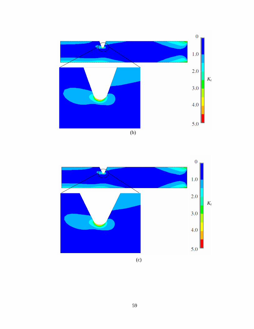
59

(b)

(c)

Kt

Kt

60

Figure 7.19. Elastic stress concentration factor, Kt, for various notch angles with other parameters at

benchmark values; (a) α = 45°, (b) α = 55°, (c) α = 65°, (d) α = 75°, (e) α = 85°.

(d)

(e)

Kt

Kt

61

These trends are depicted graphically in Figs. 7.20 and 7.21. These plots further solidify

the observation that the stresses in the notch are not highly sensitive to the notch angle.

This weak correlation is due to the fact that the geometry of the notch root is effectively

unchanged throughout the studied range of notch angles. Since the maximum stresses are

realized in a very confined vicinity of the notch root, a very minute change in geometric

configuration of the radius tip will result in minute change in stress.

Figure 7.20. Elastic stress concentration factors with respect to notch angle for different notch depths.

62

Figure 7.21. Elastic stress concentration factors with respect to notch angle for different notch root radii.

7.5 Angular Stress Distribution

The previous sections focused on how the behavior of the maximum stresses at

the notch root varies as a function of various geometric parameters of the notch. The

present section investigates the angular stress distributions about the surface of the notch.

These stress distributions are characterized by the angular location parameter β, shown in

Fig.7. 22. A value of β = 0° corresponds to the exact middle of the notch root. The

equivalent stress values of nodes along the radius of the notch were extracted along with

the Cartesian location of the nodes. The Cartesian locations were converted into angular

locations and the nodes were sorted in ascending order based on angular location through

use of a Fortran code provided in Appendix A. The resulting angular stress distribution

codes provide insight into the location within the notch root experiencing maximum

stress. In typical symmetric notch problems, the maximum stress is found at the middle

63

of the notch root; however, in the case of axisymmetrically loaded plates, the location of

the maximum stress is a function of notch geometry and location.

Figure 7.22. Angular stress distribution parameter β along the root radius of the notch.

The radial location of the notch was observed to have the greatest effect on the

angular stress distributions. This result is expected since the radial location of the notch

was shown to have the largest effect on the state of stress throughout the plate. Figure

7.23 depicts the angular distributions of the elastic stress concentration factor, Kt, for

various radial locations of the notch at otherwise benchmark conditions.

64

Figure 7.23. Angular stress distributions of Kt along the root radius of the notch for various radial notch

locations.

A number of results can be drawn from this figure with respect to the relationship

between the radial location of the notch and the magnitude and location of the maximum

equivalent stresses along the notch root. Similar to the results discussed in section 7.1, it

is shown in Fig. 7.23 that the magnitude of the stresses along the notch radius decrease as

the radial location of the notch is increased until a transition point is reached (r/a = 0.63),

after which an increase in the radial location of the notch causes a large increase in the

magnitude of the notch tip stresses. Regarding the angular location of the maximum

equivalent stress, Fig. 7.23 illustrates that this location is a negative β for radial locations

less the transition point and a positive β for radial locations after this transition point.

Interestingly, a nearly symmetric angular stress distribution is observed at this transition

point of r/a = 0.63 and is highlighted in the figure.

Nearly

symmetric

distribution

65

The relationship between the depth of the notch and the resulting angular stress

distributions was similarly explored. It was found that the relative magnitude of the

angular stress distributions decreased as the depth of the notch approached the mid-plane,

similar to the results discussed in section 7.2. This general trend is shown in Fig. 7.24.

The radial location of maximum equivalent stress was observed to be near the middle of

the notch root for shallow notches, but to diverge towards large negative angular

locations as the notch depth was increased.

Figure 7.24. Angular stress distributions along the root radius of the notch for various notch depths.

The radius of the notch was observed to have a negligible effect on the angular

location of the maximum equivalent stress. As shown in Fig. 7.23, only the magnitude of

the stress distribution was affected by notch radii. This observation is due to the fact that

a change in the radius of the notch root does not alter the location of the notch tip within

the plate, and therefore does not affect the inherent stress state corresponding to that

particular radial and axial location. As discussed earlier, changes in the location of the

66

notch tip throughout the plate affect both the magnitude and shape of the angular stress

distributions; however, changes to purely notch geometry only affect the stress

magnitude. This point is also illustrated in Fig. 7.26, in which the elastic stress

concentration factor distributions with respect to various notch angles are depicted

graphically.

Figure 7.25. Angular stress distributions along the root radius of the notch for various notch radii.

67

Figure 7.26. Angular stress distributions along the root radius of the notch for various notch angles.

7.6 Vertical Stress Distribution

The vertical stress distributions with respect to various geometric notch

parameters were investigated similarly to the angular stress distributions. The vertical

stress distribution is characterized by the normalized vertical location parameter, z/d, as

shown in Fig. 7.27. The vertical stress distribution originates at the middle of the notch

root tip and traversed to the bottom of the plate corresponding to a z/d = 0.714.

Figure 7.27. Vertical stress distribution parameter z.

z/d = 0.714

68

Both the magnitude and the distribution of the equivalent stresses ahead of the

notch were found to be greatly influenced by the radial location of the notch. The

vertical elastic stress concentration factor distributions for various radial notch locations

are shown in Fig. 7.28. The maximum stresses along this vertical line are realized at the

notch tip (z/d = -0.29). It is important to distinguish that this is the maximum stress along

this vertical line which bisects the notch root radius and may not be the maximum stress

along the notch root. The location of the maximum stress along the notch root was

discussed in section 7.5.

Figure 7.28. Stress distributions ahead of the notch for various radial notch locations.

For all the curves in Fig. 7.28, a common trend observed is that equivalent

stresses rapidly decrease from the maximum at the notch tip to the minimum value; after

which the stresses slowly increase until the bottom of the plate is reached. Similar to

results observed for the angular stress distributions with respect to the radial location, it is

shown in Fig. 7.28 that the curves corresponding to r/a = 0.57 and r/a = 0.70 are both the

69

smallest in magnitude and represent a nearly constant stress concentration factor

throughout the thickness of the plate.

The depth of the notch was shown to merely affect the magnitude of the stress

concentration factor distribution ahead of the notch. As shown in Fig. 7.29, the stress

distributions are similar in shape, but differ in the value of the maximum stress

concentration factor. Also, these curves originate at different axial locations because the

depth of the notch was the geometric parameter varied in this particular case. This is also

the reason that the axial location, z, is normalized by the height of plate, h, instead of d.

Figure 7.29. Stress distributions ahead of the notch for various notch angles.

The radius of the notch root and the angle of the notch were shown to only

slightly affect the elastic stress concentration factor distributions ahead of the notch.

These results are consistent with the previously observed results with respect to the

influence of these geometric parameters on stress in the vicinity of the notch. The stress

70

distributions ahead of the notch with respect to the radius of the notch root and the notch

angle are depicted graphically in Figs. 7.30 and 7.31, respectively.

Figure 7.30. Stress distributions ahead of the notch for various notch root radii.

Figure 7.31. Stress distributions ahead of the notch for various notch angles.

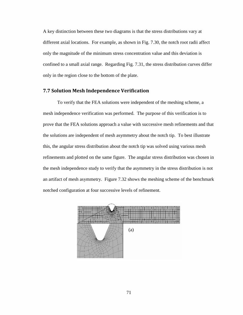
71

A key distinction between these two diagrams is that the stress distributions vary at

different axial locations. For example, as shown in Fig. 7.30, the notch root radii affect

only the magnitude of the minimum stress concentration value and this deviation is

confined to a small axial range. Regarding Fig. 7.31, the stress distribution curves differ

only in the region close to the bottom of the plate.

7.7 Solution Mesh Independence Verification

To verify that the FEA solutions were independent of the meshing scheme, a

mesh independence verification was performed. The purpose of this verification is to

prove that the FEA solutions approach a value with successive mesh refinements and that

the solutions are independent of mesh asymmetry about the notch tip. To best illustrate

this, the angular stress distribution about the notch tip was solved using various mesh

refinements and plotted on the same figure. The angular stress distribution was chosen in

the mesh independence study to verify that the asymmetry in the stress distribution is not

an artifact of mesh asymmetry. Figure 7.32 shows the meshing scheme of the benchmark

notched configuration at four successive levels of refinement.

(a)

72

Figure 7.32. Mesh of benchmark notch configuration at refinement (a) level 1, (b) level 2, (c) level 3, and

(d) level 4.

The angular stress distributions solved from each of these meshing schemes are

illustrated in Fig. 7.33. From this figure, it is evident that the angular stress distribution is

only slightly affected by the mesh refinement level and is shown to approach a common

curve with successive refinements. The level 4 mesh refinement was used throughout the

entire FEA of the current paper. It can be concluded from this mesh independence

(c)

(d)

(b)

73

analysis that the solutions of the stress distributions in the vicinity of the notch are

independent of the mesh asymmetry about the notch tip. Furthermore, it was shown that

the solution to the stress distribution approaches a value and continued levels of

refinement would not yield higher accuracy.

Figure 7.33. Angular stress distribution solutions for various mesh refinement levels.

74

8. Conclusions

In summary, relationships between v-notch stress concentration factors and notch

geometry and location were formulated through parametric finite element analysis.

Correlations between individual geometric notch parameters and resulting stress

concentration factors were mathematically modeled. Such models could be used by plate

designers to determine the necessary notch geometry for a desired stress concentration

factor. The relation formulated providing the stress concentration factor as a function of

the notch root radius was found to closely match the form of that determined by Inglis

(1913). This result suggests that further correlations between stress concentration factor

relations for simple and axisymmetric loading can be developed. In general, it was

determined that the stresses in the vicinity of the notch tip were more sensitive to changes

in notch location (r and t) than in pure notch geometry (ρ and α). This result is due to the

inherent stress dependence on the radial and axial location within the plate. A

formulation for the location of minimum equivalent stress within a smooth plate was

developed and it was observed that this location acts as a point of symmetry for stress

distributions along the radius of the notch.

75

9. Future Work

The results presented in the current paper were solved assuming a series of

idealizations and simplifications which provided a solid framework for the understanding

of the complex relationships between the stresses in the vicinity of the notch tip and the

notch geometry and location. Idealizations in the FEA such as static loading, isotropic

material, elastic behavior, and isothermal conditions allow for only approximate solutions

to be found, which cannot be readily applied to the service conditions of the component

under consideration; therefore, future studies are planned which will employ further

mechanical testing and advanced FEA to provide solutions more applicable to the actual

application of circular v-notched components.

Future mechanical testing will consist of flexural experiments of notched,

rectangular components to understand the effects of pure bending stresses on the fracture

behavior. Additionally, flexural experiments will provide correlations between simple

and axisymmetric bending. The tensile experiments conducted previously will be

repeated with multiple tests at each configuration to provide statistical certainties

associated with experimental results. Notched members will be tested at high strain rates

to simulate the impact these plate components experience in service and to further

quantify rate dependency of the mechanical properties and fracture behavior of Ultem

1000.

In regards to advanced FEA, elastic-plastic simulations will provide insights into

the strain hardening effects on the maximum stresses in the vicinity of the notch. Also,

elastic and plastic deformation distributions will be characterized within the vicinity of

76

the notch. Dynamic simulations will consider the rate dependence of Ultem 1000 and the

resulting effects on the v-notch stress concentration factors and fracture behavior. Since

in the industry application of guided projectiles the circular plate components are subject

to extreme fluctuations in heat, future numerical simulations will incorporate the known

thermal properties of Ultem 1000 and attempt to predict the resulting fracture behaviors.

Finally, studies of similar materials such as Ultem variations or custom material blends

will be conducted to determine an optimized material composition which will yield a

more predictable and controllable fracture behavior.

77

Appendix A: Codes

78

A.1 Parametric ANSYS Input File (para_notch_plate.inp)

Finish

/Clear /PREP7

/OUTPUT,junk,txt

! Specify initial, final, and increment values for parameters:

!X_ini=.5 !X_inc=.2

!X_fin=2.5

!DEP_ini=.1 !DEP_inc=.02

!DEP_fin=.3

ANG_ini=45 ANG_inc=9

ANG_fin=90

!RAD_ini=.02 !RAD_inc=.003

!RAD_fin=.05

i=1

!*DO,X_LOC_RD,X_ini,X_fin,X_inc !*DO,DEP_NTCH,DEP_ini,DEP_fin,DEP_inc

*DO,ANG_NTCH,ANG_ini,ANG_fin,ANG_inc

!*DO,RAD_NTCH,RAD_ini,RAD_fin,RAD_inc PARSAV,,parameters,txt

*IF,i,GT,1,THEN finish

/clear

/PREP7 PARRES,,parameters,txt

*ENDIF

finish

/FILNAME, 4 Parameter Study

/title, 4 Parameter Study

/prep7

/OUTPUT,junk1,txt !***********************************************************************************************************

*********

! Primary Function: !

! This input file simulates a circular plate with a concentric v-notch on the top surface subject to a static, uniform,

! axisymmetric pressure load on the top surface. Multiple parameters are independently varied and corresponding ! results are output for further analysis to provide insight into the effect each parameter has on stress ditribution

! in the vicinity of the notch.

! ! Results:

!

! The results of this simulation are output to independently named text files and include the radial, hoop, and

! equivalent stresses in the vicinity of the notch and the deflection of the center of the plate.

!

! Parametric Setup: !

! Four variables are independently varied through use of a DO LOOP, namely X_LOC_RD, DEP_NTCH, and ANG_NTCH, and

! RAD_NTCH. The results for each run are stored in individual text files: !

! Output files:

! ! The results are output into individually named text files with the following naming convention:

!

! Plate Deflection Results: DEFLECTN_"X_LOC_RD"_"DEP_NTCH"_"ANG_NTCH"_"RAD_NTCH".txt

! Locations of nodes along notch tip: NNLOC_"X_LOC_RD"_"DEP_NTCH"_"ANG_NTCH"_"RAD_NTCH".txt

! Component stresses along notch tip: NCSTR_"X_LOC_RD"_"DEP_NTCH"_"ANG_NTCH"_"RAD_NTCH".txt

79

! Principal stresses along notch tip: NPSTR_"X_LOC_RD"_"DEP_NTCH"_"ANG_NTCH"_"RAD_NTCH".txt

! Locations of nodes along vertical line: VNLOC_"X_LOC_RD"_"DEP_NTCH"_"ANG_NTCH"_"RAD_NTCH".txt ! Component stresses along vertical line: VCSTR_"X_LOC_RD"_"DEP_NTCH"_"ANG_NTCH"_"RAD_NTCH".txt

! Principal stresses along vertical line: VPSTR_"X_LOC_RD"_"DEP_NTCH"_"ANG_NTCH"_"RAD_NTCH".txt

! Locations of nodes along horizontal line: HNLOC_"X_LOC_RD"_"DEP_NTCH"_"ANG_NTCH"_"RAD_NTCH".txt ! Component stresses along horizontal line: HCSTR_"X_LOC_RD"_"DEP_NTCH"_"ANG_NTCH"_"RAD_NTCH".txt

! Principal stresses along horizontal line: HPSTR_"X_LOC_RD"_"DEP_NTCH"_"ANG_NTCH"_"RAD_NTCH".txt

! !

! Meshing Scheme and other FEM Characteristics:

! ! This input file utilizes ANSYS "free meshing" and the element size is based on the "smart size" tool

! with refinement set to level 4. Extra mesh refinement exists along areas of interest, namely the notch tip,

! the outer circumferential boundary, and the inner axial boundary. Since this is an axisymmetric analysis, only ! one half of a 2D cross section of the disk need be modeled. B.C's are set appropriately to take advantage of symmetry.

! The PLANE82 8-Node element is used in this model. This analysis is modeled as static.

! !

! Future Updates:

! ! 1. Modify code to simulate dynamice loading.

! 2. Modify code to simulate thermal loading.

! 3. Modify code to simulate elastic-plastic deformation. !

!***********************************************************************************************************

********* ! Author: Nathan Mutter

! ver. 3.4 ! Date: 12/05/09

!***********************************************************************************************************

********* ! List of Parameters and descriptions:

!***********************************************************************************************************

********* ! Input Parameters (Define system and do not change)

! ----------------

! HT_PLATE Thickness of the plate [in]

! RD_PLATE Radius of the plate [in]

! PRESSURE Evenly distributed pressure [psi]

! DENS_ULT Density of Ultem 1000 [lb/in^3] !

! Varied Parameters

! ---------------- ! X_LOC_RD Radial distance of notch tip [in] (.1<X_LOC_RD<2.9)

! DEP_NTCH Depth of the notch [in] (.1<DEP_NTCH<.4)

! ANG_NTCH Angle of notch [degrees] (60<ANG_NTCH<120) ! RAD_NTCH Radius of notch tip [in] (.03125<RAD_NTCH<.09375)

!

! Parameters Derived from Geometric Relationships ! -----------------------------------------------

! HT_NOTCH Height of the notch tip [in]

! HT_RADIU Height of the center of radius [in] ! PHI Half of angle of notch [degrees]

!***********************************************************************************************************

*********

PI = 3.14159265

*AFUN, DEG

X_LOC_RD = 1

ANG_NTCH = 60 DEP_NTCH = .15

RAD_NTCH = .035

HT_PLATE = .5 ! Thickness of the plate [in]

RD_PLATE = 3 ! Radius of the plate [in]

PRESSURE = 300 ! Evenly distributed pressure [psi]

! Specify horizontal and vertical bands for stress distributions

X1=X_LOC_RD-.02

80

X2=X_LOC_RD+.02

Y1=DEP_NTCH-.02 Y2=DEP_NTCH+.02

! Geometric relationships HT_NOTCH = HT_PLATE - DEP_NTCH

HT_RADIU = HT_NOTCH + RAD_NTCH

PHI = ANG_NTCH/2 l = DEP_NTCH*tan(PHI) ! distance of corner keypoint from center line of notch tip

r_x = RAD_NTCH*cos(PHI) ! x projection of the radius

r_y = RAD_NTCH*sin(PHI) ! y projection of the radius x = RD_PLATE - (X_LOC_RD + l) ! distance from far end of disk to corner keypoint

! Keypoints k, 1, 0.0, 0.0 ! keypoint located at (0.0, 0.0)

k, 2, RD_PLATE, 0

k, 3, RD_PLATE, HT_PLATE k, 4, 0, HT_PLATE

k, 5, X_LOC_RD, HT_RADIU

k, 6, X_LOC_RD, HT_NOTCH k, 7, X_LOC_RD + r_x, HT_RADIU - r_y

k, 8, X_LOC_RD - r_x, HT_RADIU - r_y

k, 9, X_LOC_RD + l, HT_PLATE k, 10, X_LOC_RD - l, HT_PLATE

! Lines

L, 1, 2 ! L1 connecting keypoints 1 and 2 L, 2, 3 ! L2

L, 3, 9 ! L3

L, 9, 7 ! L4 L, 8, 10 ! L5

L, 10, 4 ! L6

larc, 8, 7, 5, RAD_NTCH ! L7 arc centered at keypoint 5 with radius r connecting keypoints 8 and 7 L, 4, 1 ! L8

! Areas

AL, all ! define an area bounded by all lines

ksel,all

! Element

ET,1,PLANE82 ! axisymmetric structural element KEYOPT,1,3,1 ! turn on axisymmetric key option

! Material Properties of Ultem 100 MP, EX, 1, 420e3 ! modulus of elasticicy (psi)

MP, PRXY, 1, .35 ! poissons ratio

MP, DENS, 1, 0.046243 ! density (lb/in^3)

! Meshing of entire 2D cross section using free meshing and "smart sizing" MSHAPE, 0, 2D ! mesh with quadrilateral-shaped elements

MSHKEY, 0 ! free mesh

SMRTSIZE,3 ! refinement level 3 AMESH, 1

! Refine Mesh

LREFINE, 4,5,1,2,4,,

LREFINE, 7,7,1,2,1,, ! refine mesh along notch tip !LREFINE, 2,2,1,1 ! refine mesh along circumferential boundary

!LREFINE, 8,8,1,1 ! refine mesh along axial boundary

! Boundary Conditions

LSEL,S,LINE,,2,2,1 ! constrain movement in x direction for nodes on line 2 (circumferential boundary)

NSLL,S,1 D,ALL,UX,0

LSEL,ALL

LSEL,S,LINE,,2,2,1 ! constrain movement in y direction for nodes along line 2 (circumferential boundary)

81

NSLL,S,1

D,ALL,UY,0 LSEL,ALL

! Loads LSEL,S,LINE,,3,6,3 ! select lines 3 and 6

NSLL,S,1 ! select nodes associated with those lines

SF,all,PRES,PRESSURE ! apply uniform pressure load along top surface of plate LSEL,all

! Output files containing node locations LSEL,S,LINE,,7,7,1

NSLL,S,1

NWRITE,NNLOC_%X_LOC_RD%_%DEP_NTCH%_%ANG_NTCH%_%RAD_NTCH%_,txt, ! outputs Cartesian location of nodes along notch tip

!NSEL,S,LOC,X,X1,X2

!NWRITE,VNLOC_%X_LOC_RD%_%DEP_NTCH%_%ANG_NTCH%_%RAD_NTCH%_,txt, ! outputs Cartesian location of nodes along vertical line

!NSEL,S,LOC,Y,Y1,Y2

!NWRITE,HNLOC_%X_LOC_RD%_%DEP_NTCH%_%ANG_NTCH%_%RAD_NTCH%_,txt, ! outputs Cartesian location of nodes along horizontal line

LSEL,all

NSEL,all

FINISH

/SOLU solve

FINISH

/POST1

! Create job names for each run for each output file

DEF_JOB = 'DEF_%X_LOC_RD%_%DEP_NTCH%_%ANG_NTCH%_%RAD_NTCH%_.txt'

NNLOC_JOB = 'NNLOC_%X_LOC_RD%_%DEP_NTCH%_%ANG_NTCH%_%RAD_NTCH%_.txt' NCSTR_JOB = 'NCSTR_%X_LOC_RD%_%DEP_NTCH%_%ANG_NTCH%_%RAD_NTCH%_.txt'

NPSTR_JOB = 'NPSTR_%X_LOC_RD%_%DEP_NTCH%_%ANG_NTCH%_%RAD_NTCH%_.txt'

VNLOC_JOB = 'VNLOC_%X_LOC_RD%_%DEP_NTCH%_%ANG_NTCH%_%RAD_NTCH%_.txt'

VCSTR_JOB = 'VCSTR_%X_LOC_RD%_%DEP_NTCH%_%ANG_NTCH%_%RAD_NTCH%_.txt'

VPSTR_JOB = 'VPSTR_%X_LOC_RD%_%DEP_NTCH%_%ANG_NTCH%_%RAD_NTCH%_.txt'

HNLOC_JOB = 'HNLOC_%X_LOC_RD%_%DEP_NTCH%_%ANG_NTCH%_%RAD_NTCH%_.txt' HCSTR_JOB = 'HCSTR_%X_LOC_RD%_%DEP_NTCH%_%ANG_NTCH%_%RAD_NTCH%_.txt'

HPSTR_JOB = 'HPSTR_%X_LOC_RD%_%DEP_NTCH%_%ANG_NTCH%_%RAD_NTCH%_.txt'

! Create index files for each output file set

*CFOPEN, INDEX_DEFLECTN,txt,,append

*VWRITE, DEF_JOB %C

/OUTPUT,junk2,txt

*CFOPEN, INDEX_NNLOC,txt,,append *VWRITE, NNLOC_JOB

%C

/OUTPUT,junk3,txt *CFOPEN, INDEX_NCSTR,txt,,append

*VWRITE, NCSTR_JOB

%C /OUTPUT,junk4,txt

*CFOPEN, INDEX_NPSTR,txt,,append

*VWRITE, NPSTR_JOB %C

/OUTPUT,junk5,txt

!*CFOPEN, INDEX_VNLOC,txt,,append !*VWRITE, VNLOC_JOB

!%C

!/OUTPUT,junk6,txt !*CFOPEN, INDEX_VCSTR,txt,,append

!*VWRITE, VCSTR_JOB

!%C !/OUTPUT,junk7,txt

!*CFOPEN, INDEX_VPSTR,txt,,append

!*VWRITE, VPSTR_JOB

82

!%C

!/OUTPUT,junk8,txt !*CFOPEN, INDEX_HNLOC,txt,,append

!*VWRITE, HNLOC_JOB

!%C !/OUTPUT,junk9,txt

!*CFOPEN, INDEX_HCSTR,txt,,append

!*VWRITE, HCSTR_JOB !%C

!/OUTPUT,junk10,txt

!*CFOPEN, INDEX_HPSTR,txt,,append !*VWRITE, HPSTR_JOB

!%C

!/OUTPUT,junk11,txt

! Deflection data

KSEL,S,KP,,4,4,1 NSLK,S

/OUTPUT,DEF_%X_LOC_RD%_%DEP_NTCH%_%ANG_NTCH%_%RAD_NTCH%_,txt ! outputs y deflection of center of

plate for each run PRNSOL,U,Y

/OUTPUT,junk12,txt

! Notch data

LSEL,S,LINE,,7,7,1

NSLL,S,1 /OUTPUT,NCSTR_%X_LOC_RD%_%DEP_NTCH%_%ANG_NTCH%_%RAD_NTCH%_,txt ! outputs component stress data

along notch tip for each run PRNSOL,S,COMP

/OUTPUT,NPSTR_%X_LOC_RD%_%DEP_NTCH%_%ANG_NTCH%_%RAD_NTCH%_,txt ! outputs principle stress data along

notch tip for each run PRNSOL,S,PRIN

/OUTPUT,junk13,txt

LSEL,all NSEL,all

! Vertical range data

!NSEL,S,LOC,X,X1,X2

!/OUTPUT,VCSTR_%X_LOC_RD%_%DEP_NTCH%_%ANG_NTCH%_%RAD_NTCH%_,txt ! outputs component stress data

along vertical band for each run !PRNSOL,S,COMP

!/OUTPUT,VPSTR_%X_LOC_RD%_%DEP_NTCH%_%ANG_NTCH%_%RAD_NTCH%_,txt ! outputs principal stress data

along vertical band for each run !PRNSOL,S,PRIN

!/OUTPUT,junk14,txt

!LSEL,all !NSEL,all

! Horizontal range data !NSEL,S,LOC,Y,Y1,Y2

!/OUTPUT,HCSTR_%X_LOC_RD%_%DEP_NTCH%_%ANG_NTCH%_%RAD_NTCH%_,txt ! outputs component stress data

along horizontal band for each run !PRNSOL,S,COMP

!/OUTPUT,HPSTR_%X_LOC_RD%_%DEP_NTCH%_%ANG_NTCH%_%RAD_NTCH%_,txt ! outputs principal stress data

along horizontal band for each run !PRNSOL,S,PRIN

!/OUTPUT,junk15,txt

!LSEL,all !NSEL,all

PLDISP,0

PLESOL,S,X,0

i=i+1

FINISH

*ENDDO !*ENDDO

!*ENDDO

!*ENDDO

83

A.2 FORTRAN Data Extractor Code (data_extract.f90)

program data_extractor

!!!!!!!!!!!!!!!!!!!!!!!!!!!!!!!!!!!!!!!!!!!!!!!!!!!!!!!!!!!!!!!!!!!!!!!!!!!!!!!!

! Program Function: ! This program extracts results from simulation output files and writes the

! data in tabulated format to one output file.

! ! Author: Nathan Mutter

! Date: 2-20-2010

! Version: 1.3 !

! Future Updates:

! 1. ! 2.

!!!!!!!!!!!!!!!!!!!!!!!!!!!!!!!!!!!!!!!!!!!!!!!!!!!!!!!!!!!!!!!!!!!!!!!!!!!!!!!!

! Array and variable declaration:

character*40, dimension (700) :: NCSTR_JOB character*40, dimension (700) :: NPSTR_JOB

character*40, dimension (700) :: DEFLECTN_JOB

character(len=80) line character(len=80) line_clean_c

character(len=80) line_clean_p

character(len=80) line_clean_d integer :: job_num, job_num_max

real :: MX_RAD_STRES, MX_AXI_STRES, MX_HOP_STRES, MX_PRIN_STRES, MX_EQ_STRES, DEFLECTN, MX_SHR_STRES

! Determine number of files to be read and store as job_num_max:

open (1, file='INDEX_NCSTR.txt', status='old') job_num_max=0

do

read(1,100,iostat=io) if (io .eq. -1) then

go to 1

else job_num_max = job_num_max+1

endif

end do 1 continue

close(1)

! Create job name arrays from each job name index file:

! INDEX_NCSTR

do job_num=1,job_num_max

open (2, file='INDEX_NCSTR.txt', status='old') read (2,100) line

NCSTR_JOB(job_num)=line

enddo

! INDEX_NPSTR

do job_num=1,job_num_max open (3, file='INDEX_NPSTR.txt', status='old')

read (3,100) line

NPSTR_JOB(job_num)=line enddo

84

! INDEX_DEFLECTN do job_num=1,job_num_max

open (4, file='INDEX_DEFLECTN.txt', status='old')

read (4,100) line DEFLECTN_JOB(job_num)=line

enddo

close(2)

close(3)

close(4)

! Open individual simulation results files, extract data of interest

! and store in arrays:

! Open component stress result files and extract the max Radial, Axial

! Hoop and Shear stresses. do job_num =1,job_num_max

open(6,file=NCSTR_JOB(job_num),status='old')

2 read (6,100,end=3) line_clean_c if (line_clean_c(2:4).eq.'MAX') then

read (6,100) junk

read (6,110) MX_RAD_STRES, MX_AXI_STRES, MX_HOP_STRES, MX_SHR_STRES

continue

else goto 2

end if 3 continue

! Open principle stress result files and extract the max first principle stress.

open(7,file=NPSTR_JOB(job_num),status='old')

4 read (7,100,end=5) line_clean_p if (line_clean_p(2:4).eq.'MAX') then

read (7,100) junk

read (7,120) MX_PRIN_STRES, MX_EQ_STRES

continue

else

goto 4 end if

5 continue

! Open deflection result files and extract deflection of center plate.

open (8, file=DEFLECTN_JOB(job_num), status='old') 6 read (8,100,end=7) line_clean_d

if (line_clean_d(2:4).eq.'MAX') then

read (8,100) junk read (8,130) DEFLECTN

continue

else goto 6

end if

7 continue

! Write data in tabulated form to an output file:

open (9, file='CLEAN_DATA.txt', status='unknown')

write (9,140) DEFLECTN_JOB(job_num)(5:30), MX_RAD_STRES, MX_AXI_STRES, &

& MX_HOP_STRES, MX_SHR_STRES, MX_PRIN_STRES, MX_EQ_STRES, DEFLECTN

enddo

! Formats

100 format(a80) 110 format(8X F10.2,1X F10.2, 3X F10.2, 2X F10.2)

120 format (7X F10.2,41X F10.2)

130 format (8X F7.3)

85

140 format (a25,7(6X F10.3))

close(6)

close(7) close(8)

close(9)

end

86

A.3 FORTRAN Stress Distribution Code (stress_dist.f90)

program stress_distributions

!!!!!!!!!!!!!!!!!!!!!!!!!!!!!!!!!!!!!!!!!!!!!!!!!!!!!!!!!!!!!!!!!!!!!!!!!!!!!!!!

! Program Function: ! This program extracts shear stress and von Mises stress values from nodes along

! the radius of the notch and converts the nodal Cartesian coordinates into

! polar coordinates centered above the notch tip with a constant radius equal to ! the notch tip radius. This program also extracts shear and von Mises stress

! values from nodes along a vertical line from the notch tip to the bottom of the

! plate. The stresses and nodal locations for both the angular and vertical ! distribution cases are written to separate text files for each parametric

! combination.

! ! Author: Nathan Mutter

! Date: 2-27-2010

! Version: 1.0 !

! Future Updates:

! !

!

! !!!!!!!!!!!!!!!!!!!!!!!!!!!!!!!!!!!!!!!!!!!!!!!!!!!!!!!!!!!!!!!!!!!!!!!!!!!!!!!!

! Array and variable declaration

! If varying X_LOC_RD:

!REAL,PARAMETER :: X_INI=0.5, X_FIN=2.5, X_INC=0.2

!REAL,PARAMETER :: X_SIZE=((X_FIN-X_INI)/X_INC)+1 !REAL,DIMENSION(1:X_SIZE) :: X_LOC_RD

REAL :: RAD_NTCH

! If varying RAD_NTCH:

!REAL,PARAMETER :: RAD_INI=0.02, RAD_FIN=0.05, RAD_INC=0.003

!REAL,PARAMETER :: RAD_SIZE=((RAD_FIN-RAD_INI)/RAD_INC)+1 !REAL,DIMENSION(1:RAD_SIZE) :: RAD_NTCH

REAL :: X_LOC_RD

CHARACTER*40, DIMENSION(100) :: NCSTR_JOB, NPSTR_JOB, C_NCSTR_JOB, &

C_NPSTR_JOB, NNLOC_JOB, VCSTR_JOB, VPSTR_JOB, C_VCSTR_JOB, C_VPSTR_JOB, &

VNLOC_JOB, ANG_DIST_JOB, VERT_DIST_JOB CHARACTER (len=80) :: line

INTEGER :: job_num, job_num_max, NODE_NUM, NNLOC_NODE, NPSTR_NODE, VNLOC_NODE, &

VPSTR_NODE REAL :: X_COORD, Y_COORD, ANG_SEQV, ANG_SHEAR, ANG_SINT, ANG_MX_SHEAR, ANGLE, VERT_SEQV, &

VERT_SINT, VERT_MX_SHEAR, VERT_SHEAR

!!!!!!!!!!!!!!!!!!!!!!!!!!!!!!!!!!!!!!!!!!!!!!!!!!!!!!!!!!!!!!!!!!!!!!!!!!!!!!!!

! Determine number of jobs to be read based on index file:

open (1, file='INDEX_NCSTR.txt', status='old') job_num_max=0

do

read(1,100,iostat=io) if (io .eq. -1) then

go to 1

else job_num_max= job_num_max+1

87

endif

end do 1 continue

close(1)

!!!!!!!!!!!!!!!!!!!!!!!!!!!!!!!!!!!!!!!!!!!!!!!!!!!!!!!!!!!!!!!!!!!!!!!!!!!!!!!!

! Define geometric parameters neccessary for angular coordinate calculation: ! 1. If varying the DEP_NTCH or ANG_NTCH then X_LOC_RD and RAD_NTCH are

! constants and the below do loop declarations are not neccessary.

! 2. If varying X_LOC_RD then RAD_NTCH is constant. ! 3. If varying RAD_NTCH then X_LOC_RD is constant.

! 4. Depending on which notch parameters are being varied, the correct "ANGLE"

! formula must be chosen in the body of the code (see ***). !!!!!!!!!!!!!!!!!!!!!!!!!!!!!!!!!!!!!!!!!!!!!!!!!!!!!!!!!!!!!!!!!!!!!!!!!!!!!!!!

!

! VARY X_LOC_RD:

RAD_NTCH=.035

!do i=1,job_num_max

!X_LOC_RD(i)=X_INI+((i-1)*X_INC)

!enddo

! OR

! VARY NTCH_RAD:

X_LOC_RD=1

!do i=1,job_num_max !RAD_NTCH(i)=RAD_INI+((i-1)*RAD_INC)

!enddo

!!!!!!!!!!!!!!!!!!!!!!!!!!!!!!!!!!!!!!!!!!!!!!!!!!!!!!!!!!!!!!!!!!!!!!!!!!!!!!!!

! Create job name arrays from each job name index file:

! INDEX_NCSTR do job_num=1,job_num_max

open (2, file='INDEX_NCSTR.txt',status='old')

read (2,100) line NCSTR_JOB(job_num)=line

enddo

! INDEX_NPSTR

do job_num=1,job_num_max

open (3, file='INDEX_NPSTR.txt',status='old') read (3,100) line

NPSTR_JOB(job_num)=line

enddo

! INDEX_NNLOC

do job_num=1,job_num_max open (4, file='INDEX_NNLOC.txt',status='old')

read (4,100) line

NNLOC_JOB(job_num)=line enddo

! INDEX_VCSTR do job_num=1,job_num_max

open (6, file='INDEX_VCSTR.txt',status='old')

read (6,100) line VCSTR_JOB(job_num)=line

enddo

88

! INDEX_VPSTR

do job_num=1,job_num_max open (7, file='INDEX_VPSTR.txt',status='old')

read (7,100) line

VPSTR_JOB(job_num)=line enddo

! INDEX_VNLOC do job_num=1,job_num_max

open (8, file='INDEX_VNLOC.txt',status='old')

read (8,100) line VNLOC_JOB(job_num)=line

enddo

!!!!!!!!!!!!!!!!!!!!!!!!!!!!!!!!!!!!!!!!!!!!!!!!!!!!!!!!!!!!!!!!!!!!!!!!!!!!!!!!

! Clean stress files and rename:

do job_num=1,job_num_max

open(unit=9, file=NCSTR_JOB(job_num), status='old')

open(unit=10,file='C_'//NCSTR_JOB(job_num), status='unknown')

do while (.true.) read (9,100,end=5) line

do i=1,80

if (line(i:i).eq.' ') goto 2 if (line(i:i).eq.'0') goto 4

if (line(i:i).eq.'1') goto 4 if (line(i:i).eq.'2') goto 4

if (line(i:i).eq.'3') goto 4

if (line(i:i).eq.'4') goto 4 if (line(i:i).eq.'5') goto 4

if (line(i:i).eq.'6') goto 4

if (line(i:i).eq.'7') goto 4 if (line(i:i).eq.'8') goto 4

if (line(i:i).eq.'9') goto 4

goto 3

4 continue

write (10,100) line

goto 3 2 continue

enddo

3 continue enddo

5 continue

open(unit=11, file=NPSTR_JOB(job_num), status='old')

open(unit=12,file='C_'//NPSTR_JOB(job_num), status='unknown')

do while (.true.) read (11,100,end=9) line

do i=1,80

if (line(i:i).eq.' ') goto 6 if (line(i:i).eq.'0') goto 8

if (line(i:i).eq.'1') goto 8

if (line(i:i).eq.'2') goto 8 if (line(i:i).eq.'3') goto 8

if (line(i:i).eq.'4') goto 8

if (line(i:i).eq.'5') goto 8 if (line(i:i).eq.'6') goto 8

if (line(i:i).eq.'7') goto 8

if (line(i:i).eq.'8') goto 8 if (line(i:i).eq.'9') goto 8

goto 7

8 continue write (12,100) line

goto 7

6 continue enddo

7 continue

enddo

89

9 continue

open(unit=13, file=VCSTR_JOB(job_num), status='old')

open(unit=14,file='C_'//VCSTR_JOB(job_num), status='unknown') do while (.true.)

read (13,100,end=13) line

do i=1,80 if (line(i:i).eq.' ') goto 10

if (line(i:i).eq.'0') goto 12

if (line(i:i).eq.'1') goto 12 if (line(i:i).eq.'2') goto 12

if (line(i:i).eq.'3') goto 12

if (line(i:i).eq.'4') goto 12 if (line(i:i).eq.'5') goto 12

if (line(i:i).eq.'6') goto 12

if (line(i:i).eq.'7') goto 12 if (line(i:i).eq.'8') goto 12

if (line(i:i).eq.'9') goto 12

goto 11 12 continue

write (14,100) line

goto 11 10 continue

enddo

11 continue enddo

13 continue

open(unit=15, file=VPSTR_JOB(job_num), status='old')

open(unit=16,file='C_'//VPSTR_JOB(job_num), status='unknown') do while (.true.)

read (15,100,end=17) line

do i=1,80 if (line(i:i).eq.' ') goto 14

if (line(i:i).eq.'0') goto 16

if (line(i:i).eq.'1') goto 16

if (line(i:i).eq.'2') goto 16

if (line(i:i).eq.'3') goto 16

if (line(i:i).eq.'4') goto 16 if (line(i:i).eq.'5') goto 16

if (line(i:i).eq.'6') goto 16

if (line(i:i).eq.'7') goto 16 if (line(i:i).eq.'8') goto 16

if (line(i:i).eq.'9') goto 16

goto 15 16 continue

write (16,100) line

goto 15 14 continue

enddo

15 continue enddo

17 continue

enddo

close(2) close(3)

close(4)

close(6) close(7)

close(8)

close(9) close(10)

close(11)

close(12) close(13)

close(14)

close(15)

90

close(16)

!!!!!!!!!!!!!!!!!!!!!!!!!!!!!!!!!!!!!!!!!!!!!!!!!!!!!!!!!!!!!!!!!!!!!!!!!!!!!!!!

! Extract SEQV, shear stress, and X_COORD of the nodes along notch radius. Convert

! to angular location around radius of notch and write to ANG_DIST.txt.

do job_num=1,job_num_max

do while (.true.)

open(2,file='C_'//NCSTR_JOB(job_num),status='old') open(3,file='C_'//NPSTR_JOB(job_num),status='old')

open(4,file=NNLOC_JOB(job_num),status='old')

read(2,110,end=25) NODE_NUM, ANG_SHEAR

18 read(3,120,end=19) NPSTR_NODE, ANG_SINT, ANG_SEQV if (NPSTR_NODE .eq. NODE_NUM) then

go to 20

else go to 18

endif

19 print*, 'Node number not found' 20 continue

ANG_MX_SHEAR=ANG_SINT/2

21 read(4,130,end=22) NNLOC_NODE, X_COORD

if (NNLOC_NODE .eq. NODE_NUM) then go to 23

else

go to 21 end if

22 print*, 'Node number not found'

23 continue

! ******************************************************************************

!!!!!!!!!!!!!!!!!!!!!!!!!!!!!!!!!!!!!!!!!!!!!!!!!!!!!!!!!!!!!!!!!!!!!!!!!!!!!!!! ! Convert cartesian coordinates into polar:

!

! Depending on which parameters of the notch are being varied, choose the ! appropriate "ANGLE" statement below and "comment" out the other two:

! If varying DEP_NTCH or ANG_NOTCH, use below statement:

ANGLE=ASIN((X_COORD-X_LOC_RD)/RAD_NTCH)*(180/3.1416)

! If varying X_LOC_RD, use below statement:

!ANGLE=ASIN((X_COORD-X_LOC_RD(job_num))/RAD_NTCH)*(180/3.1416)

! If varying RAD_NTCH, use below statement:

!ANGLE=ASIN((X_COORD-X_LOC_RD)/RAD_NTCH(job_num))*(180/3.1416)

!!!!!!!!!!!!!!!!!!!!!!!!!!!!!!!!!!!!!!!!!!!!!!!!!!!!!!!!!!!!!!!!!!!!!!!!!!!!!!!!

! ******************************************************************************

! Write ANG_DIST text files for each job:

open(6,file='ANG_DIST_'//NCSTR_JOB(job_num),status='unknown')

write(6,140) NODE_NUM, X_COORD, ANGLE, ANG_SHEAR, ANG_MX_SHEAR, ANG_SEQV

enddo

25 continue

enddo

91

close(2) close(3)

close(4)

close(6) !!!!!!!!!!!!!!!!!!!!!!!!!!!!!!!!!!!!!!!!!!!!!!!!!!!!!!!!!!!!!!!!!!!!!!!!!!!!!!!!

! Extract SEQV, shear stress, and Y_COORD of the nodes along a vertical line from ! the notch tip to the bottom of the plate and write results to VERT.DIST.txt.

do job_num=1,job_num_max

do while (.true.)

open(2,file='C_'//VCSTR_JOB(job_num),status='old')

open(3,file='C_'//VPSTR_JOB(job_num),status='old')

open(4,file=VNLOC_JOB(job_num),status='old')

read(2,110,end=30) NODE_NUM, VERT_SHEAR

38 read(3,120,end=31) VPSTR_NODE, VERT_SINT, VERT_SEQV

if (VPSTR_NODE .eq. NODE_NUM) then

go to 40 else

go to 38

endif 39 print*, 'Node number not found'

40 continue VERT_MX_SHEAR=VERT_SINT/2

31 read(4,150,end=32) VNLOC_NODE, Y_COORD if (VNLOC_NODE .eq. NODE_NUM) then

go to 33

else go to 31

end if

32 print*, 'Node number not found'

33 continue

! Write VERT_DIST text files for each job:

open(6,file='VERT_DIST_'//NCSTR_JOB(job_num),status='unknown')

write(6,160) NODE_NUM, Y_COORD, VERT_SHEAR, VERT_MX_SHEAR, VERT_SEQV

enddo

30 continue

enddo

!!!!!!!!!!!!!!!!!!!!!!!!!!!!!!!!!!!!!!!!!!!!!!!!!!!!!!!!!!!!!!!!!!!!!!!!!!!!!!!!

! Formats:

100 format(a80)

110 format(4X I4, 36X F10.2) 120 format(4X I4, 38X F9.2,3X F9.2)

130 format(4X I4, 2X F10.8)

140 format(I4,5X F8.5,4(5X F8.2)) 150 format(4X I4, 20X F20.17)

160 format(I4,5X F8.5,3(5X F8.2))

!!!!!!!!!!!!!!!!!!!!!!!!!!!!!!!!!!!!!!!!!!!!!!!!!!!!!!!!!!!!!!!!!!!!!!!!!!!!!!!!

end

92

Appendix B: Mechanical Testing Photographs and Fractographs

93

Figure B.1. Side view of fracture surfaces of smooth specimens from tensile experiments at (a) 0.5 mm/s,

(b) 0.05 mm/s, and (c) 0.005 mm/s.

Figure B.2. Isometric view of fracture surfaces of smooth specimens from tensile experiments at (a) 0.5

mm/s, (b) 0.05 mm/s, and (c) 0.005 mm/s.

Figure B.3. SEM fractograph of smooth specimen from tensile test at 0.5 mm/s.

(a) (b) (c)

(a) (b) (c)

94

Figure B.4. Side view of fracture surfaces of blunt notched specimens from tensile experiments at (a) 0.5

mm/s, (b) 0.05 mm/s, and (c) 0.005 mm/s.

Figure B.5. Isometric view of fracture surfaces of blunt notched specimen from tensile experiments at (a)

0.5 mm/s, (b) 0.05 mm/s, and (c) 0.005 mm/s.

Figure B.6. SEM fractographs showing smooth ridge of blunt notched specimen tested at 0.5 mm/s.

(a) (b) (c)

(a) (b) (c)

95

Figure B.7. SEM fractographs showing crack initiation of blunt notched specimen tested at 0.5 mm/s.

Figure B.8. SEM fractographs showing smooth ridge of blunt notched specimen tested at 0.05 mm/s.

Figure B.9. SEM fractographs showing crack initiation of blunt notched specimen tested at 0.05 mm/s.

96

Figure B.10. SEM fractographs showing smooth ridge of blunt notched specimen tested at 0.005 mm/s.

Figure B.11. SEM fractographs showing crack initiation of blunt notched specimen tested at 0.005 mm/s.

Figure B.12. Side view of fracture surfaces of sharp notched specimens from tensile experiments at (a) 0.5

mm/s and (b) 0.05 mm/s.

(a) (b)

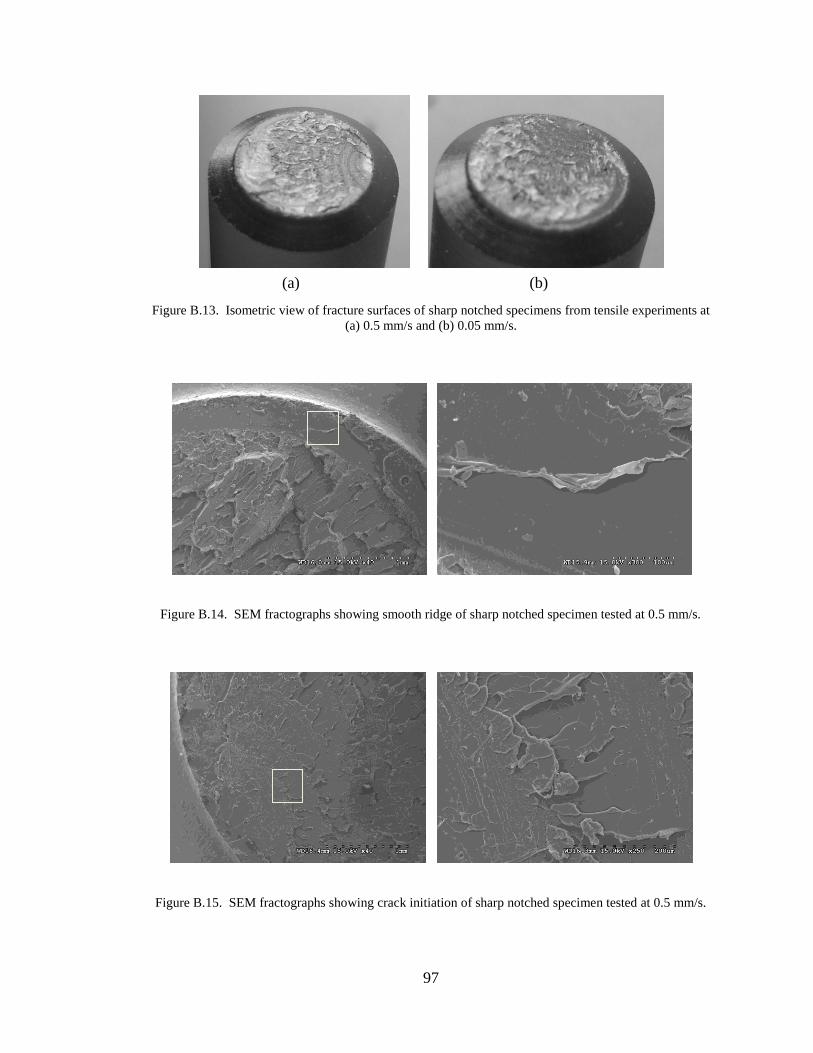
97

Figure B.13. Isometric view of fracture surfaces of sharp notched specimens from tensile experiments at

(a) 0.5 mm/s and (b) 0.05 mm/s.

Figure B.14. SEM fractographs showing smooth ridge of sharp notched specimen tested at 0.5 mm/s.

Figure B.15. SEM fractographs showing crack initiation of sharp notched specimen tested at 0.5 mm/s.

(a) (b)

98

Figure B.16. SEM fractographs showing smooth ridge of sharp notched specimen tested at 0.05 mm/s.

Figure B.17. SEM fractographs showing crack initiation of sharp notched specimen tested at 0.05 mm/s.

99

References

1. Apple, F. J., and Koerner, D. R. “Stress Concentration Factors for U-Shaped,

Hyperbolic and Rounded V-Shaped Notches.” ASME Paper 69-DE-2, Eng. Soc.

Library, United Eng. Center, New York. (1969).

2. Bijwe, J., Tewari, U. S., and Vasudevan, P. “Friction and Wear Studies of Bulk

Polyetherimide.” Journal of Materials Science, 25(1) (1991): 548-556.

3. Bordonaro, C. M., and Krempi, E. “The Rate-Dependent Mechanical Behavior of

Plastics: A Comparison between 6/6 Nylon, Polyetherimide and

Polyetheretherketone.” Proceedings – 1993 American Society of Mechanical

Engineers Winter Annual Meeting, New Orleans, LA. November 28 – December

3.

4. Facca, A. G., Kortschot, M. T., and Yan, N. “Predicting the Tensile Strength of

Natural Fibre Reinforced Thermoplastics.” Composites Science and Technology,

67(6) (2007): 2454-2466.

5. Greenhalgh, E. S., Failure Analysis and Fractography of Polymer Composites.

Boca Raton: Woodhead Publishing Limited, 2009.

6. Inglis, C. E. “Stresses in a Plate Due to the Presence of Cracks and Sharp

Corners.” Trans. Inst. Naval Architects, A221 (1913): 219-230.

7. Johnson, R., and Jafry, S. “Ultem Polyetherimide Resin for the Medical

Industry.” Proceedings – Society of Petroleum Engineers Annual Western

Regional Meeting, (1998). Anaheim, CA. January 19-22.

100

8. Kim, K., and Ye, L. “Effects of Thickness and Environmental Temperature on

Fracture Behavior of Polyetherimide (PEI).” Journal of Materials Science, 39(4)

(2004): 1267-1376.

9. Leven, M. M., and Frocht, M. M. “Stress Concentration Factors for a Single

Notch in a Flat Plate in Pure and Central Bending.” Proc. System Engineering

Society of Australia, 11(2) (1953): 179.

10. Neuber, H. Kerbspannungslehre, 2nd

ed. Berlin: Springer, 1958; Translation,

Theory of Notch Stresses, Washington, D.C.: Office of Technical Services, Dept.

of Commerce, 1961.

11. Noda, N. A., and Takase, Y. “Stress concentration formulae useful for any shape

of notch in a round test specimen under tension and under bending.” Fatigue and

Fracture of Engineering Materials and Structures, 22(12) (1999): 1071-1082.

12. Pecht, M., and Wu, X. “Characterization of Polyimides Used in GE-High Density

Interconnects.” International Society for the Advancement of Material and

Process Engineering Electronics Conference, 7.2 (1994): 432-445. Parsippany,

NJ. June 20-23.

13. Pilkey, W. D. Peterson’s Stress Concentration Factors Second Edition. New

York: Wiley-Interscience, 1997.

14. Reddy, J. N. Theory and Analysis of Elastic Plates. Philadelphia, PA: Taylor &

Francis, 1999.

15. Rodriguez, J. E., Brennan, F. P., and Dover, W. D. “Minimization of Stress

Concentration Factors in Fatigue Crack Repairs.” International Journal of

Fatigue, 20(10) (1998): 719-725.

101

16. SABIC Innovative Plastics Ultem 1000 Data Sheet. Retrieved June 15, 2008,

from

<http://www.matweb.com/search/datasheet.aspx?matguid=4b8cf67e11ee4c08aee

413e45643f956&ckck=1>

17. Savage, T. “Ultem Resin Plays a Dual Cost Saving and Safety Role in Aviation.”

Aircraft Engineering and Aerospace and Technology, 60(4) (1988): 24-25.

18. Schmidt, R. “Finite Axisymmetric Deflections of a Loosely Clamped Circular

Plate Subjected to a Two-Parameter Distributed Load.” The Journal of Industrial

Mathematics Society, 34(1) (1984): 89-98.

19. Schobig, M., Bierogel, C., Grellmann, W., and Mecklenburg, T. “Mechanical

Behavior of Glass-Fiber Reinforced Thermoplastic Materials Under High Strain

Rates.” Polymer Testing, 27(7) (2008): 893-900.

20. Smmazcelik, T., Coban, O., Bora, M. O., Gunay, V., and Curgul, I. “The Effects

of Thermal Cycles on the Impact Fatigue Properties of Thermoplastic Matrix

Composites.” Applied Composite Materials, 15(2) (2008): 99-113.

21. Stokes, V., and Nied, H. “Lateral Strain Effects During the Large Extension of

Thermoplastics.” Polymer Engineering and Science, 28(19) (1988): 1209-1218.

22. Swallowe, G. M., Mechanical Properties and Testing of Polymers. Dordrecht:

Kluwer Academic Publishers, 1999.

23. Szilard, R. Theories and Analysis of Plates. New Jersey: Prentice-Hall, 1974.

24. Timoshenko, S. P., and Gere, J. M. Theory of Elastic Stability. New York:

McGraw Hill, 1961.

102

25. Tlilan, H. M., Sakai, N., and Majim, T. “Effect of Notch Depth on Strain-

Concentration Factor of Rectangular Bars with Single-Edge Notch Under Pure

Bending.” International Journal of Solids and Structures, 43(3) (2006): 459-474.

26. Tou, G., and Zihui, X. “Mean Stress/Strain Effect on Fatigue Behavior of an

Epoxy Resin.” International Journal of Fatigue, 29(12) (2007): 2180-2190.

27. Ugural, A.C. Stresses in Plates and Shells Second Edition. New York: McGraw-

Hill, 1999.

28. Wang, C. M., Nazmul, I. M., and Wang, Q. “Exact Bending Solutions of

Axisymmetric Reissner Plates in Terms of Classical Thin Plate Solutions.”

Advances in Structural Engineering, 7(2) (2004): 129-145.

29. Wescott, R., Semple, B., and Heller, M. “Stress Analysis of Near Optimal Surface

Notches in 3D Plates.” Journal of Mechanical Design, 127(6) (2005): 1173-1183.