Stress, Balance Equations, and Isostasy - · PDF fileStress, Balance Equations, and Isostasy We deﬁne stress to consider forces acting at depths, and derive the equations of mass,

Chapter 3

Stress, Balance Equations, andIsostasy

We define stress to consider forces acting at depths, and derive the equations of mass,linear momentum, angular momentum, and energy conservation. Very slow tectonicmovements allow us to neglect inertia force and simplify the equation of motion to abalance equation. Isostasy is the most basic but important application of force balanceequations to tectonics.

3.1 Definition of stress

Suppose that a square pole is composed of five rectangler solids (Fig. 3.1(a)). If the pole bears aload at the top and base, the parts may push each other across the bounding planes. Parts A and Bmay push each other with that load. However, parts C and D may push each other with much lessforce. Force across a plane in a solid depends on the direction of the plane.

In order to consider a force exerted on a rock mass, suppose there is a surface element δS onthe mass, and a unit vector N normal to the surface and pointing outward indicates the attitude ofthe surface element (Fig. 3.1(b)). In addition, let the vector δF be the traction force acting on theelement. The force may increase with the area δS so that we define a vector quantity t(N ) as theforce per unit area exerted there. N is in parentheses because the force depends on the attitude of thesurface element. The quantity is called a stress vector. Mathematically, the stress vector is definedby

t(N ) = limδS→0

δF

δS. (3.1)

The stress vector and its components are expressed in the units Nm−2 = pascals (Pa)1.

1The same units are used to count pressure. 1 bar = 105 Pa = 1000 hPa = 0.1 MPa. Engineering literature often uses theunits kgf/cm2 which are approximately equal to 0.98 MPa. The unit dyn cm−2 is used in older literature. It is converted bythe factor 1 Pa = 10 dyn cm−2.

59

60 CHAPTER 3. STRESS, BALANCE EQUATIONS, AND ISOSTASY

Figure 3.1: (a) A square pole loaded at the top and base is composed of five rectangular solids, Athrough E. (b) A rock mass is pulled from the adjacent mass with the force δF on an element of thesurface δS. A unit vector N indicates the attitude of the surface element. (c) Stress vector t(N ) andCartesian coordinates O-123 whose third axis is parallel to the unit normal N .

Consider a surface element δS with the unit, outward normal N , to which the third axis ofCartesian coordinates O-123 is adjusted (Fig. 3.1(b) and (c)). Let e(i) be the ith base vector of thecoordinates, then we write

t(N ) = S31e(1) + S32e

(2) + S33e(3), (3.2)

whereS31, S32 andS33 are the components of the stress vector t(N ), that is, t(N ) = (S31, S32, S33)T.The stress vector depends on the direction of the surface on which it acts. The first subscript ‘3’ in-dicates accordingly that the surface is normal to the third coordinate axis and its outward normalpoints positive direction of the axis. The second subscript distinguishes the components of the stressvector. A stress component normal to the surface on which it acts is known as the normal stress onthe surface, whereas the component tangent to the surface is known as shear stress. GeneralizingEq. (3.2), the components of stress vectors acting on a surface elements normal to the coordinateaxes, we have

Sij = tj(e(i)). (3.3)

We define the stress tensor from the components as

S =

⎛⎝ S11 S12 S13

S21 S22 S23

S31 S32 S33

⎞⎠ · · · components of t(e(1)

)· · · components of t

(e(2)

)· · · components of t

(e(3)

).

(3.4)

The limit in Eq. (3.1) indicates that stress vector is defined at each point on an infinitesimally smallsurface. The diagonal components are the normal stresses acting on a surface element normal to thecoordinate axes, while the other components represents shear stresses acting on the surface elements.

Sign conventions Figure 3.2(a) shows the positive direction of those components. Since we havedefined the unit vector N as being the outward normal to the surface on which the stress vector is

3.1. DEFINITION OF STRESS 61

Figure 3.2: Sign convention in continuum mechanics (a, b) and solid earth science (c, d). Arrowsindicate the direction of the positive stress components acting on a cube whose surfaces are parallelto the coordinate planes. (a) A stress component is positive when it acts in the positive directionof the coordinate axis, and on a surface of the cube whose outward normal points in the one of thepositive coordinate directions. (b) A stress component is positive when its direction is opposite tothat of (a). � and ⊗ indicate vectors pointing to this and opposite sides of the page, respectively.

defined, the opposite faces of a cube have the unit vectors in the opposite directions. Accordingly,the normal stress on the faces has the opposite positive directions, that is, the normal stresses arepositive in sign if the cube is under a tensional stress (Fig. 3.2(b)). Compressive stresses havenegative normal stresses.

We have seen that the strain tensor E has positive diagonal components if the length parallel tocoordinate axes become larger. Therefore, it is natural that positive stress components correspondto positive strain components. However, compressive stresses are common in the crust due to over-burden pressure. It is the sign convention in solid-earth science to define the sign of stress as beingpositive for compression, opposite to the sign convention of continuum mechanics (Table 3.1). Ac-cordingly, we will use the symbol r for the stress tensor with positive components for compressionto describe tectonic models. Positive directions of the components of r are shown in Fig. 3.2(c) and


Table 3.1: Symbols and signs used in this book.

Stress Unit Normal Vector Strain

Continuum Mechanics S (tension = +) N (outward) E (elongation = +)Solid-Earth Science r (compression = +) n (inward) e (shortening = + )

Figure 3.3: Direction of the unit normal vectors n and N at the surface of a rock mass.

(d). The stress tensor r should be used with the inward normal n (Fig. 3.3), where

S = −r, N = −n. (3.5)

Stress components in cylindrical coordinates Cylindrical coordinatesO-rθz are sometimes con-venient (Fig. 3.4). Transformation between the cylindrical and rectangular Cartesian coordinatesO-xyz is given by the equations,

x = r cos θ, y = r sin θ, z = z

r2 = x2 + y2, θ = tan−1(y/x).

Stress components in the coordinate systems are transformed by the two sets of equations

σrr = σxx cos2 θ + σyy sin2 θ + 2σxy sin θ cos θ, (3.6)

σθθ = σxx sin2 θ + σyy cos2 θ − 2σxy sin θ cos θ, (3.7)

σrθ = (σyy − σxx) sin θ cos θ + σxy(cos2 θ − sin2 θ). (3.8)

3.2 Cauchy’s stress formula

It is seen from Eq. (3.3) that ti(e(j))= Sji =

∑k Sjke

(i)k . Therefore, we have

t(e(i)) = ST · e(i). (3.9)

3.2. CAUCHY’S STRESS FORMULA 63

Figure 3.4: Stress components in the cylindrical coordinates O-rθ.

Note that the choice of frame of reference, the base vectors of which are e(i), is arbitrary. Equation(3.9) is generalized as follows: the stress vector acting on a surface element with the unit outwardnormal N is

t(N ) = ST ·N , (3.10)

where N may be oblique to the coordinate axes2. This is called Cauchy’s stress formula. For thesign convention of solid-earth science we have the the equivalent formula

t(n) = rT · n. (3.11)

If t(N ) is the traction on a body at its surface element with the normal N , the adjacent body has theoutward normal −N at the surface element. The action-reaction law requires that

t(N ) = −t(−N) = −t(n), (3.12)

which is shown in Fig. 3.3.

Normal and shear stresses Normal and shear stresses are the components of t(n) parallel andnormal to n, respectively. Thus,

Normal stress: σN = t(n) · n, (3.13)

Shear stress: σS =√

|t(n)|2 − σ2N. (3.14)

Since the vector n points inward at the surface of a rock mass (Fig. 3.3), σN is positive if the mass ispushed inward at the surface. By contrast, the normal stress defined by the equation

SN = t(N ) ·N (3.15)

is positive for tension. The shear stress for this sign convention is

SS =√|t(N )|2 − SN2 .

2Equation (3.10) is demonstrated via the force balance equation [134], which is introduced in §3.3. However, axiomaticcontinuum mechanics defines a stress tensor as the linear transformation from t(N ) to t(N ), rather than the force per unitarea on the surface elements parallel to coordinate planes. The interested reader will find more information in [243].


The vector σN(n) = σNn has a magnitude obviously equal to the normal stress σN and is parallelto n. If σN is positive, σN(n) points inward at the surface of the rock in question. The vector σN(n)is obtained by the orthogonal projection of t(n) onto the line parallel to n, so that the projectorP‖(n) = nn (Eq. (C.37)) is used to describe the vector:

σN(n) = P‖(n) · t(n) =(nn) · r · n =

[n · (r · n)

]n. (3.16)

On the other hand, σS(n) is defined as the vector that has a magnitude equal to the shear tractionand indicates the direction of the shear traction at the surface element of the mass. The elementaryorthogonal projector P⊥(n) = I − nn (Eq. (C.38)) is useful:

σS(n) = P⊥(n) · t(n) =(I − nn

) · t(n) = r · n − [n · (r · n)]n = t(n) − tN(n). (3.17)

Hydrostatic pressure From Eq. (3.11), let us derive a useful equation for tectonics: the tensorialformulation of hydrostatic state of stress. Consider the stress tensor defined by

r = p I, (3.18)

where I and p are the unit tensor and a scalar quantity. Coordinate rotation by Q transforms the stressas r′ = Q · r · QT = Q · (p I) · QT = pQ · QT = p I = r, indicating that the stress defined by Eq.(3.18) is isotropic, that is, independent from orientations. The state of stress is anisotropic if thereis the dependence.

In this case, the force acting on a surface element dS is t(n)dS = (r · n)dS = (pdS)n, whichis perpendicular to the surface and pointing inward with a constant magnitude of pdS. The stressvector is parallel to n for hydrostatic stress state: shear stress always vanishes. Therefore, Eq. (3.18)is known as the hydrostatic state of stress, and p is hydrostatic pressure. The equation S = −p Iexpresses the same stress for the sign convention of continuum mechanics. Hydrostatic pressureconstricts a body: it shrinks with a similar figure with the original one if the body is homogeneousinside. If the body is subject to an anisotropic stress, the shape may change.

3.3 Force balance

Tectonic motion to create a large-scale geologic structure is very slow. Forces acting on a rock massat depth may be thought of being balanced at every moment. Accordingly, we shall derive balanceequations for forces, and derive vertical stress at depth.

There are two categories of forces: surface force per unit area of the surface t and body force perunit mass X. The former was discussed in the last section. The latter acts on all the internal elementsof a body from its exterior. Examples are gravity and electromagnetic forces. As an example, gravityis written as the vector

X = (0, 0, g)T, (3.19)

where g is gravitational accerelation and the third coordinate axis points vertically downward. Bodyforce per unit volume is ρX.

3.3. FORCE BALANCE 65

3.3.1 Equation of motion

Consider a rock mass defined by a volume V and a closed surface S. Body and surface forces, Xand t(N ) act on every portion in the body and on the surface, respectively. If the forces are balanced,we have

0 =∫S

t(N ) dS +∫V

ρX dV. (3.20)

Since∫Vρv dV is the total linear momentum of the rock mass, the material derivative

DDt

∫V

ρv dV

represents the inertia force. Therefore, the equation of motion of the body is

DDt

∫V

ρv dV =∫S

t(N ) dS +∫V

ρX dV. (3.21)

The surface integral in the left-hand side of Eq. (3.21) is transformed into a volume integral withGauss’s divergence theorem (Eq. (C.63)). In addition, combining Eq. (3.10), we obtain

DDt

∫V

ρv dV =∫V

∇ · ST dS +∫V

ρX dV. (3.22)

In this case the order of D/Dt and integral is exchangable3 so that we have∫V

(ρv − ∇ · ST − ρX) dV = 0.

Since the choice of the volume is arbitrary, the integrand must vanish to satisfy this equation. Con-sequently, we obtain the differential form of

ρv = ∇ · ST + ρX or ρv = −∇ · rT + ρX. (3.23)

If the forces are balanced, we have

0 = ∇ · ST + ρX or 0 = −∇ · rT + ρX. (3.24)

The indicial notation of Eq. (3.24) is

0 =∑j

∂Sji

∂xj+ ρXi or 0 = −

∑j

∂σji

∂xj+ ρXi. (3.25)

3If V0 and V are the initial and instantaneous volumes that the rock mass occupies, respectively, at time t = 0 and t,the exchangeability is demonstrated as follows. The initial volume V0 does not depend on time, so that the operator D/Dtcan be included in the integral over V0. In addition, because of V = JV0 where J is the Jacobian, the initial and temporaldensities, ρ0 and ρ, are related to each other as ρ = ρ0/J . The initial one does not depend on time, either. That is,Dρ0/Dt = D(ρJ )/Dt = 0. Therefore,

DDt

∫Vρv dV =

DDt

∫V0

ρvJ dV0 =∫V0

[v · D(ρJ )

Dt+ ρJ

Dv

Dt

]dV0 =

∫V0

ρDv

DtJ dV0 =

∫Vρ

Dv

DtdV.


Based on Eq. (3.24), we shall derive a simple but important quantity for tectonics. Supposethat the ground surface is flat and there is no horizontal density variation. Rocks are subject to thegravitational force shown in Eq. (3.19). Defining z-axis vertically downward from sea level, theforce balance in this direction is obtained from Eq. (3.24) as

∂σxz∂x

+∂σyz

∂y+∂σzz∂z

= ρ(z)g,

where density, ρ(z), is the function of depth, z. Since there is no horizontal variation at all, the firstand second terms in the above equation vanish. We therefore have

∂σzz∂z

= ρ(z)g.

Integrating both sides, we obtain

σzz =∫ zh

ρ(ζ)g dζ, (3.26)

where h is altitude. This equation enables us to calculate the vertical stress σzz from the densityprofile ρ(z). If g is constant over the depth range in question, Eq. (3.26) becomes σzz = g

∫ zhρ(ζ) dζ .

The integral in the right-hand side of this equation is the mass of the vertical column with the unitcross-section of the height from the surface to the depth z. Therefore, σzz is the stress at the base ofthe column due to its own weight4. The vertical stress by the weight is called overburden stress. Ifdensity can be assumed to be constant, the overburden at the depth z is simply

pL = ρgz. (3.27)

We have found how the vertical stress σzz is determined. What are the other stress components?Areas of compressional and extensional tectonics may have different stress states. Stress may notonly have spatial but also tempral variations, which are represented by components other than thevertical one. However, it is convenient to define a reference stress state for later discussions. Al-though choice of the reference is arbitrary, the isotropic stress

r = pL I (3.28)

is often used for the reference in the models of tectonics, where

pL =∫ zh

ρ(ζ)g dζ (3.29)

is the overburden at depth z. This is the overburden with the same dimension with pressure. Equation(3.28) has the same form as Eq. (3.18), so that the stress indicated by Eq. (3.28) is known aslithostatic stress, and pL is called lithostatic pressure.

3.4. SYMMETRY OF STRESS TENSOR 67

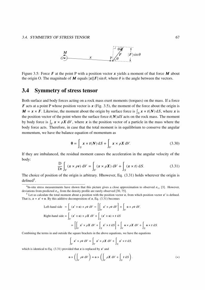
Figure 3.5: Force F at the point P with a position vector x yields a moment of that force M aboutthe origin O. The magnitude of M equals |x||F | sin θ, where θ is the angle between the vectors.

3.4 Symmetry of stress tensor

Both surface and body forces acting on a rock mass exert moments (torques) on the mass. If a forceF acts at a point P whose position vector is x (Fig. 3.5), the moment of the force about the origin isM = x × F . Likewise, the moment about the origin by surface force is

∫Sx × t(N ) dS, where x is

the position vector of the point where the surface force t(N )dS acts on the rock mass. The momentby body force is

∫Vx × ρX dV , where x is the position vector of a particle in the mass where the

body force acts. Therefore, in case that the total moment is in equilibrium to conserve the angularmomentum, we have the balance equation of momentum as

0 =∫S

x × t(N ) dS +∫V

x × ρX dV. (3.30)

If they are imbalanced, the residual moment causes the acceleration in the angular velocity of thebody:

DDt

∫V

(x × ρv) dV =∫V

(x × ρX) dV +∫S

(x × t) dS. (3.31)

The choice of position of the origin is arbitrary. Hhowever, Eq. (3.31) holds wherever the origin isdefined5.

4In-situ stress measurements have shown that this picture gives a close approximation to observed σzz [3]. However,deviations from predicted σzz from the density profile are rarely observed [30, 75].

5 Let us calculate the total moment about a position with the position vector o, from which position vector x′ is defined.That is, x = x′ + o. By this additive decomposition of x, Eq. (3.31) becomes

Left-hand side =∫V

(x′ + o) × ρv dV =

[∫Vx′ × ρv dV

]+∫V

o × ρv dV,

Right-hand side =∫V

(x′ + o) × ρX dV +∫S

(x′ + o) × t dS

=

[∫Vx′ × ρX dV +

∫Sx′ × t dS

]+∫V

o × ρX dV +∫S

o × t dS.

Combining the terms in and outside the square brackets in the above equations, we have the equations∫Vx′ × ρv dV =

∫Vx′ × ρX dV +

∫Sx′ × t dS,

which is identical to Eq. (3.31) provided that x is replaced by x′ and

o ×(∫

Vρv dV

)= o ×

(∫VρX dV +

∫St dS

). (�)


It is important for discussions in the rest of this book that the stress tensor is symmetric:

S = ST, r = rT. (3.32)

These formulas hold for both static and dynamical problems unless there is neither “couple stress”nor “body torque”. The former is the surface force acting on a body to rotate it about the axisperpendicular to the object surface, and the latter is the distributed moment in the body6. Equation(3.32) is derived from the conservation of angular momentum7.

Plane Stress It is a basic theorem in linear algebra that all the eigenvalues are of real for a real,symmetric matrix. In addition, the eigenvectors are perpendicular to each other. If one and only oneof the eigenvalues is zero, a state of plane stress is said to exist. In that case, taking coordinate axesparallel to the eigenvectors, the stress tensor is written as

S =

⎛⎝S1 0 00 S2 00 0 0

⎞⎠ ,

where S1 and S2 are non-zero eigenvalues of S. The physical interpretation of the stress state isthat traction always vanishes on a plane perpendicular to the eigenvector corresponding to the zeroeigenvalue. This is demonstrated by substituting N = (0, 0, 1)T into t(N ) = ST · N . It should benoted that plane strain and plane stress do not go together for most cases (§7.1.3).

3.5 Conservation of energy

Let us derive an equation governing temperature changes from the conservation of energy. Multi-plying both sides of Eq. (3.23) by v, we have∫

V

ρv · a dV =∫V

v · (∇ · ST) dV +∫V

ρv ·X dV, (3.33)

where V stands for the volume that the rock mass in question occupies. The left-hand side of thisequation is rewritten as∫

V

ρv · a dV =∫V

ρv · v dV =DDt

∫V

ρv · v

2dV =

DDt

∫V

ρ|v|22

dV = K.

The symbol K stands for the total kinetic energy, so that K is the rate of its increase. On the otherhand, the integrand v ·(∇·ST) in the first term in the right-hand side of Eq. (3.33) has the components

vi∂Sji

∂xj=∂(viSji)∂xj

− ∂vi∂xj

Sji =∂(viSji)∂xj

− (Dij + ωij)Sji,

This is identical to the cross-product of the constant vector o and Eq. (3.22), so that Eq. (�) is valid for any o. Therefore, Eq.(3.31) holds wherever the origin is chosen.

6See advance continuum mechanics books such as [132].7The derivation needs a tricky calculation. See, for example, [134].

3.5. CONSERVATION OF ENERGY 69

where Lij and ωij are stretching and spin tensors, respectively. Therefore, Eq. (3.33) is rewritten as

K +∫V

D : S dV =∫V

∇(v · S) dV −∫V

W : S dV +∫V

ρv ·X dV. (3.34)

Since W = (ωij) is antisymmetric we have W : S = 0. Combining this and Eq. (3.34), we obtain

K +∫V

D : S dV =∫V

∇(v · S) dV +∫V

ρv ·X dV. (3.35)

Converting the first term on the right-hand side of this equation into a surface integral by Gauss’sdivergence theorem, we obtain the energy conservation equation

K +∫V

D : S dV =∫S

[v · t(N )] dS +∫V

ρv ·X dV. (3.36)

Energy equals the product of force and distance, so that the rate of energy change equals the productof force and velocity. The right-hand side of Eq. (3.36) indicates the energy that the rock massaccepts from outside. The second term on the left-hand side is the energy dissipation due to thedeformation of the mass against the stress S. The dissipated energy is transformed to thermal orinternal energy. Let e be the internal energy per unit mass, then the internal energy per unit volumeis equal to ρe, and ∫

V

ρe dV =∫V

D : S dV. (3.37)

Therefore, the energy conservation equation is rewritten as

DDt

∫V

ρ

(v2

2+ e

)dV =

∫S

v · t(N ) dS +∫V

ρv ·X dV. (3.38)

The left-hand side of this equation represents the energy increase of the rock mass, and the right-handside indicates the work done by its outside.

Equation (3.38) was derived from the equation of motion multiplied by velocity. That is, only thebalance of kinetic energy was taken into account. However, vertical motion of a rock mass causescooling or heating of the mass. Temperature is an important factor in controlling the mechanicalproperties of rocks. Accordingly, heat transfer is important in understanding the mechanical aspectof tectonics.

Heat flux is defined by the amount of heat that passes through a unit area in a unit of time. Theheat flux is a vector quantity, so let us use the symbol q for the quantity. The heat energy passingthrough the surface dS of a rock mass in a unit time equals N ·q. Substituting this into the right-handside of Eq. (3.38), we have

DDt

∫V

ρ

(v2

2+ e

)dV =

∫S

v · t(N ) dS +∫V

ρv ·X dV −∫S

N · q dS. (3.39)


Using Gauss’s divergence theorem again, the last term in this equation is converted to a volumeintegral, and we combine all terms into the form

∫V

(· · · ) dV = 0. Since the volume V is arbitrary,this equation is satisfied only if

DDt

(v2

2+ e

)= ∇ · (S · v − q

)+ ρX · v. (3.40)

This is called the energy equation. Combining Eqs. (3.40) and (3.33), we have

e = −∇ · q + ∇ · (S · v) − v · (∇ · S).

Components of the first and second terms in the right-hand side are∑i,j

[∂(Sijvj)∂xi

− vi∂Sij

∂xj

]=∑i,j

Sij∂vi∂xj

= S : (∇v).

Therefore, we finally obtain the equation

ρe = S : (∇v) − ∇ · q. (3.41)

3.6 Self gravitational, spherically symmetric body

The direct objects of geological observations occupy shallow levels in the Earth. However, thoseobjects sometimes provide constraints on ancient global changes including planetary differentiation.The differentiation occurred at the beginning of planetary evolution, so that later geological processeshave erased all traces of the event in the Earth. However, satellites and terrestrial planets smaller thanthe Earth have geological structures that evidence the early history of the planetary bodies.

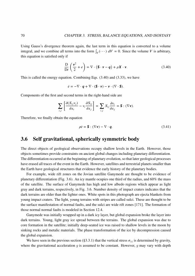
For example, wide rift zones on the Jovian satellite Ganymede are thought to be evidence ofplanetary differentiation (Fig. 3.6). An icy mantle ocupies one third of the radius, and 60% the massof the satellite. The surface of Ganymede has high and low albedo regions which appear as lightgray and dark terrains, respectively, in Fig. 3.6. Number density of impact craters indicates that thedark terrains are older than the lighter ones. White spots in this photograph are ejecta blankets fromyoung impact craters. The light, young terrains with stripes are called sulci. These are thought to bethe surface manifestation of normal faults, and the sulci are wide rift zones [171]. The formation ofthose normal normal faults is modeled in Section 12.4.

Ganymede was initially wrapped up in a dark icy layer, but global expansion broke the layer intodark terrains. Young, light gray ice spread between the terrains. The global expansion was due tocore formation in the satellite; initially deep-seated ice was raised to shallow levels in the moon bysinking rocks and metalic materials. The phase transformation of the ice by decompression causedthe global expansion.

We have seen in the previous section (§3.3.1) that the vertical stress σzz is determined by gravity,where the gravitational acceleration g is assumed to be constant. However, g may vary with depth

3.6. SELF GRAVITATIONAL, SPHERICALLY SYMMETRIC BODY 71

Figure 3.6: Surface of Ganymede, the largest Jovian satellite with a radius of 2640 km. The circularregion labeled “E” is the palimpsest Epigeous, an old and degraded large impact basin 350 km indiameter. Voyager image, 0370J2-001. Courtesy of NASA.

in the real Earth. Accordingly, in this section we study the depth-dependence of g and lithostaticpressure.

Firstly, let us assume a density distribution with spherical symmetry, and M (r) be the mass


within the distance r from the center. The gravitational acceleration at the radius is

g(r) =GM (r)r2

, (3.42)

where G = 6.67 × 10−11 Nm2 kg−2 is the gravitational constant. If density at the radius is ρ(r), wehave

M (r) =∫ r

04πr′2ρ(r′) dr′. (3.43)

Combining Eqs. (3.42) and (3.43), we obtain the gravitational acceleration as a function of r as

g(r) =G

r2

∫ r0

4πr′2ρ(r′) dr′. (3.44)

Scondly, pressure p at r is obtained from the force balance equation (Eq. (3.25)). As the forcein this case has merely originated from the self-gravity of the spherically symmetric body, there isno horizontal variation in the stress field. Equation (3.25) is rewritten for the spherical coordinatesO-rθφ as

0 = −∂σrr∂r

− 1r

∂σθr∂θ

− 1r sin θ

∂σφr

∂φ− ρg, (3.45)

where both ρ and g are the functions r and the latter is given by Eq. (3.44). The gravity term ρg

in Eq. (3.45) is negative in sign, because gravity points downward, i.e., in the direction of −r. Ifthe spherical body is composed of viscous fluid at rest, the state of stress in the body is hydrostatic.In this case, shear stresses σθr and σφr vanish, and in Eq. (3.45) σrr should be replaced by thehydrostatic pressure p. Consequently, we have

dpdr

= −ρg. (3.46)

As ρ and g are always positive in sign, Eq. (3.46) indicates that p should decrease with r.Let us calculate g and p as the functions of r for the two cases in Fig. 3.7. Density in the layers

is assumed to be constant. The former is a simple model for the Moon. Our Moon had its ownmagnetic field a few billion years ago, suggesting that there was a melted metalic core at the center.However, the core is so small that it is difficult to estimate its dimension. Accordingly, we assumethe Moon to be a rocky spherical body with a constant density ρ = 3.3 × 103 kg m−3 to roughlyestimate the gravitational acceleration and pressure at depths8. In the case of a constant density ρ,the integral in Eq. (3.43) results in M (r) = 4πρr3/3, and we obtain

g(r) =4π3Gρr. (3.47)

8The Moon has a less dense crust than the mantle. However, the mean thickness of the crust is less than 100 km, twoorders of magnitude smaller than the radius of the Moon, which is about 1740 km. Accordingly, the crust is neglected in thisestimation.

3.6. SELF GRAVITATIONAL, SPHERICALLY SYMMETRIC BODY 73

Figure 3.7: Pressure p and gravitational acceleration g versus distance r from the center of a spher-ically symmetric body. (a) Single-layer model Moon with a constant density with the parametersρ = 3.3×103 kg m−3 andR = 1740 km. (b) Two-layer model Earth with the parameters ρm = 4×103

kg m−3, ρc = 10 × 103 kg m−3, Rc = 3490 km, and R = 6380 km.

It follows that gravitational acceleration for a constant density, spherically symmetric body is pro-portional to the distance from the center (Fig. 3.7(a)). Substituting Eq. (3.47) into (3.46), wehave

dpdr

= −4πGρ2

3r.

Using the boundary condition p = 0 at r = R, where R stands for the radius of the Moon, we obtainthe pressure distribution

p(r) =2π3ρ2G(R2 − r2). (3.48)

The density distribution in the Earth is roughly simulated by a two-layer model, as about halfthe radius of the Earth is occupied by a high density, metalic core at the center and the crust isnegligibly thin compared to the core and mantle. We do not take into account the tiny densitydifference between the inner and outer cores. Let R and RC be the radius of the Earth and the core,respectively, then the density is

ρ =

{ρC (r ≤ RC)ρm (RC < r ≤ R).

(3.49)

Gravitational acceleration in the core is the same as Eq. (3.47) and we have

g(r) =4π3GρCr (r ≤ RC),


where ρC is the density of the core. If that of the mantle is ρm, gravitational acceleration in the mantleis obtained by using Eqs. (3.44) and (3.49) as

g(r) =4πG

3

[ρmr + (ρC − ρm)

R3C

r2

](RC < r ≤ R).

Figure 3.7(b) shows g(r) for a double-layered model Earth. It is seen in this figure that g is roughlyconstant in the upper mantle. The models of tectonics in the following sections of this book dealwith the crust and the upper mantle, so that we will always assume that gravitational acceleration isconstant.

Pressure distribution in the model Earth is given by integrating Eq. (3.46) as

p(r) =4π3Gρm (ρC − ρm)R3

C

(1r− 1R

)+

2π3Gρ2

m

(R2 − R2

C

)+

2π3Gρ2

C

(R2

C − r2) (r < RC) ,

p(r) =4π3GρmR

3c (ρC − ρm)

(1Rc

− 1R

)+

2π3Gρ2

m

(R2 − r2) (RC < r < R) .

The gravitational acceleration and pressure in the model Earth are calculated with the values, ρm =4.0 × 103 kg m−3, ρcore = 10 × 103 kg m−3, Rc = 3490 km, R = 6380 km, and G = 6.7 × 10−11

Nm2 kg−2, and are shown in Fig. 3.7. It is seen that gravitational acceleration is more or less constantin the upper mantle. Therefore, the acceleration is always assumed to be constant in the followingsections of this book.

3.7 Isostasy

Buoyancy is an important force to drive tectonics. The crust has smaller density than the underlyingmantle so that the crust is subject to buoyancy forces from the mantle and is floating on it. Thetectonic thinning and thickening of the crust cause the subsidence and uplift of the surface. We willderive Archimedes’ principle from the force balance equation.

Suppose a solid body is immersed in a fluid with a density of ρ (Fig. 3.8). The body and fluid areassumed to stand still so that all forces acting on the body are balanced. The force balance equation(Eq. (3.20)) in this case is

0 =∫S

t(n) dS +∫V

X dV, (3.50)

where V and S are the volume and surface of the body. The first and second terms on the right-handside of this equation represent surface force from the fluid to the body and gravitational force (Eq.(3.19)), respectively. The buoyancy force exerting on the body is the former. The traction at thesurface is pressure, p. That is, t(n) = pn. Using Gauss’s divergence theorem, the surface integral is

3.7. ISOSTASY 75

Figure 3.8: Schematic illustration to explain Archimedes’ principle.

converted to a volume integral. Therefore, the buoyancy term is rewritten as∫S

pn dS = −∫V

∇p dV. (3.51)

A minus sign is placed on the right-hand side of this equation because the unit normal n is definedinward, unlike the case of Eq. (C.63). It should be noted that the integration on the right-hand side ofEq. (3.51) is taken inside the body, although p is not the pressure in the body but fluid pressure at thesurface. Since the fluid is at rest, the pressure depends only on the depth z. The pressure gradient,∇p, and the gravity term in Eq. (3.50) have no horizontal component. Therefore, an equation ofscalar quantities is enough to consider the vertical force balance of this system. Let Fb be buoyancy,and ρ be constant, then Eq. (3.50) is converted to the equation

Fb = −ρ∫V

dV = −ρV,

where the negative signs came from the definition of the force Fb that is positive upward. Thisequation stands for Archimedes’ principle: an object completely immersed in a fluid experiences anupward buoyant force equal in magnitude to the weight of the fluid displaced by the object.

The concept of isostasy is derived from that principle. Suppose the structure shown in Fig. 3.9,where a continental crust with a thickness of tc is floating on a mantle. According to Archimedes’principle, the buoyancy force exerted at the base of the crust is the weight of the mantle displacedby the part of the crust that is immersed in the mantle. The weight is ρmghcS, where ρm the mantledensity and S the area of the base. Other symbols are shown in Fig. 3.9. The gravitational forcethat the crustal block experiences is ρcgtcS, which should be balanced with the buoyancy force.Therefore, we have

ρcgtc = ρmghc. (3.52)


Figure 3.9: A simple model for a continental crust floating on a mantle.

This equation says that the lithostatic pressure at the level of the base is spatially constant. If densityvariations in the upper mantle are not negligible, this level should be taken to be deeper. The litho-spheric plate that is composed of a crust and upper mantle is often envisaged as floating on a fluidasthenosphere. Rocks behave as fluid in a geological timescale, if they have high temperature. Onthe other hand, if the lower mantle is heated to become fluid, upper crustal blocks with smaller den-sities float on it. The level is placed in the middle of the crust. The level under which rocks behaveas fluid and they cannot support a lithostatic pressure difference is called the depth of compensation.

A simple model of isostasy asserts that overburden is constant at a depth of compensation. Thefollowing equation represents this concept:∫ dc

surfaceρg dz = constant, (3.53)

where dc is the depth of compensation, and the z-axis is defined downward with the sea level at z = 0.If an offshore region is considered, the lower bound of this integral is taken to be at sea level to takeinto account the load of the ocean water. The integral is spatially or temporarily constant. When itis thought to be temporarily constant, we can calculate subsidence and uplift accompanied by thetemporal variation of density distribution at depths, i.e., vertical movements that are recognized fromstratigraphy give constraints to the variation.

Equation (3.53) represents a one-dimensional model of isostasy, where density variations onlyalong the z direction are taken into account. This idea is sometimes referred to as local isostasycompared to regional isostasy that is introduced in Section 8.1. In the latter model, horizontal densityvariations are explicitly included in its equation.

In the rest of this chapter we will use a simple isostatic model to calculate topography and verticaltectonic movements.

3.8 Balance between ocean and continent

There are two tectonic classes of regions, continents and oceans. This division is reflected in thefrequency distribution of the height or water depth of the surface of the solid Earth (Fig. 3.10).

3.8. BALANCE BETWEEN OCEAN AND CONTINENT 77

Figure 3.10: Cumulative frequency distribution of the altitude of the surface of the solid Earth.

There are apparently two modes at about 1 km above and 3–4 km below sea level. They correspondto the average altitude of the continents at 0.84 km and the average depth of oceans at 3.4 km.

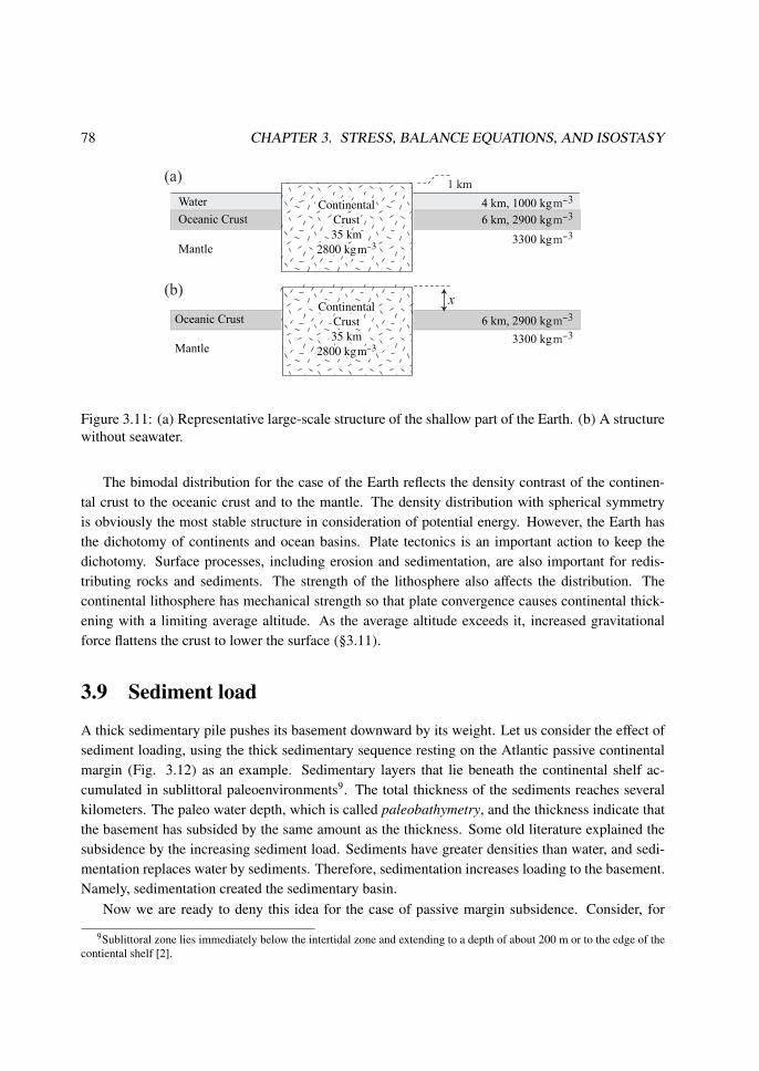
Let us see that the two levels are in isostatic equilibrium [78]. Assuming g = 10 ms−1 andthe depths and densities shown in Fig. 3.11(a) for representative continent and ocean, we have theoverburden at the Moho depth under the continent

pL = ρcgto = 0.98 GPa. (3.54)

The overburden under the ocean basin at the same level is

pL = ρwgb + ρogto + ρmg (tc − h − b − to) ≈ 1.006 GPa, (3.55)

which is about the same as that under the continent (Eq. (3.54)). Therefore, continents and oceansare roughly in isostatic equilibrium.

Seawater pushes the oceanic crust downward by its weight, and pushes the continents upward.What if the Earth loses oceans by extreme global warming? The average continental altitude fromthe average oceanic surface, x in Fig. 3.11(b), would have been decreased. Neglecting other factorsincluding thermal expansion of rocks, the overburden at the level of continental Moho is

pL = ρcgto + ρmg (tc − to − x) .

Equating this pressure and that in Eq. (3.54), we obtain x = (tc − to) (ρm − ρc)/ρm ≈ 3.3 km.The frequency distribution of global topographic height, hypsometry, is used to investigate the

tectonics of terrestrial planets and moons. If impact cratering was the most significant process forshaping the surface of a planetary body, the resultant frequency distribution would be somethinglike a normal distribution. In spite of the existence of numberless impact craters, the Moon has twomodes in its distribution. They correspond to highlands and maria, suggesting that this distinctionwas formed through some global processes.


Figure 3.11: (a) Representative large-scale structure of the shallow part of the Earth. (b) A structurewithout seawater.

The bimodal distribution for the case of the Earth reflects the density contrast of the continen-tal crust to the oceanic crust and to the mantle. The density distribution with spherical symmetryis obviously the most stable structure in consideration of potential energy. However, the Earth hasthe dichotomy of continents and ocean basins. Plate tectonics is an important action to keep thedichotomy. Surface processes, including erosion and sedimentation, are also important for redis-tributing rocks and sediments. The strength of the lithosphere also affects the distribution. Thecontinental lithosphere has mechanical strength so that plate convergence causes continental thick-ening with a limiting average altitude. As the average altitude exceeds it, increased gravitationalforce flattens the crust to lower the surface (§3.11).

3.9 Sediment load

A thick sedimentary pile pushes its basement downward by its weight. Let us consider the effect ofsediment loading, using the thick sedimentary sequence resting on the Atlantic passive continentalmargin (Fig. 3.12) as an example. Sedimentary layers that lie beneath the continental shelf ac-cumulated in sublittoral paleoenvironments9. The total thickness of the sediments reaches severalkilometers. The paleo water depth, which is called paleobathymetry, and the thickness indicate thatthe basement has subsided by the same amount as the thickness. Some old literature explained thesubsidence by the increasing sediment load. Sediments have greater densities than water, and sedi-mentation replaces water by sediments. Therefore, sedimentation increases loading to the basement.Namely, sedimentation created the sedimentary basin.

Now we are ready to deny this idea for the case of passive margin subsidence. Consider, for

9Sublittoral zone lies immediately below the intertidal zone and extending to a depth of about 200 m or to the edge of thecontiental shelf [2].

3.9. SEDIMENT LOAD 79

Figure 3.12: Crustal structure of the southern Baltimore Canyon Trough, Atlantic margin of NorthAmerica. LJ, Lower Jurassic; MJ, Middle Jurassic; UJ, Upper Jurassic; LK, Lower Cretaceous; UK,Upper Cretaceous; T, Tertiary. Simplified from [101].

Figure 3.13: Sedimentary basin subsidence by sediment load.

simplicity, a constant density for sediments ρs. If an ocean basin with an initial depth of b is filledup with sediments (Fig. 3.13), the final thickness of the sedimentary pile x is given by the isostasyequation

ρwgb + ρcgtc + ρmg (x − b) = ρsgx + ρcgtc.

The left- and right-hand sides of this equation correspond to the left and right columns, respectively,in Fig. 3.13. Therefore, we obtain

x =

(ρm − ρw

ρm − ρs

)b. (3.56)

The density of sediment depends on the lithology. Using a representative value ρs = 2.3 × 103

kg m−3, we have x = 2.3b. If excessive sediments are supplied from the hinterland, the sedimentswould be exported to the lower reaches. For the case of the thick shallow marine sequence on thepassive continental margin, b ≤ 0.2 km results in x ≈ 0.5 km. Therefore, the basement subsidedactively, not passively, because of the sediment load (§3.14).

It is necessary to grasp subsidence history, and not only the initial water depth and final sediment


thickness, to understand the mechanism of subsidence. Quantitative stratigraphy provides a way toreconstuct the history.

3.10 Quantitative stratigraphy

The subsidence history of a sedimentary basin is an observable function of time. Quantitative stratig-raphy or geohistory analysis is the technique used to reconstruct the history from formations, whereisostatic balance plays an important role. The result of the analysis designates the vertical componentof the tectonic movements.

For this purpose, the necessary data are the present depth, lithology, porosity, sedimentation age,the paleobathymetry of formations, and the eustatic sea level curve for the period covering the agesof the formations. The paleobathymetry is estimated from sedimentary structures characteristic for acertain depth such as hammocky cross-stratification, which indicates the depths were so shallow thatthe sedimentation was affected by surface waves. Some kinds of molluscs and benthic foraminiferslive on the ocean bottom at certain water depths so that benthic fossils are another indicator ofpaleobathymetry. Figure 3.14 shows the paleo topography inferred from those kinds of data aroundJapan. The Japanese island arcs experienced vertical movements on the order of kilometers in theMiocene [263, 272].

The basic idea of geohistory analysis is that the sum of the formation thickness and paleo-bathymetry gives the depth to the basement from the present sea level, and applies several cor-rections. There are three key factors for the accumulation of thick sedimentary pile. Firstly, tectonicsubsidence is necessary to form a container of sediments. Secondly, sediment supply is impor-tant. If the supply is scarce, a sediment-starved basin is the result. Thirdly, eustasy affects notonly paleobathymetry but also sedimentation. A eustatic rise is equivalent to tectonic subsidencefor sedimentation. We can abstract vertical tectonic movements from a sedimentary basin by takinginto account these and additional factors. The mathematical procedure employed for this purpose iscomparable to the stripping of formations from the top to lowest stratigraphic horizons (Fig. 3.15),so that it is known as the backstripping technique.

The density of rocks is important for isostasy. Sediments lose their porosity and get a largerdensity while they are buried. Pores between sedimentary particles are usually filled with forma-tion fluids that are mostly water. For example, mudstone has a porosity of some 50% shortly afterdeposition, However, increasing compactness of the particles expels the fluids during burial, i.e.,compaction occurs. The porosity φ is the volume fraction of a pore. The porosity of mudstone isless than 10% at depths of a few kilometers. The total volume of sedimentary particles in a unitvolume is 1 − φ. It is known that porosity of sedimentary rocks decreases roughly exponentiallywith depth,

φ = φ0 e−Cζ , (3.57)

where ζ is depth from the ocean bottom. The parameters φ0 andC depend on lithology. Accordingly,it is assumed that the parameters are determined for rock types at depths, e.g., in boreholes.

3.10. QUANTITATIVE STRATIGRAPHY 81

Figure 3.14: Paleo topography around Japanese islands from 23 to 15 Ma inferred from sedimentaryenvironments. Benthic fossils and depositional facies are the keys for estimating the environment.The Japan arc drifted to form the Japan Sea backarc basin in the Early Miocene. The paleo posi-tion of the arc before 15 Ma, when the opening was completed, is controversial so that the paleoenvironments are indicated on the present map of this region.

If a formation has a horizonally infinite extension, the porosity reduction results in the thinning ofthe formation. Consider a formation with an initial thickness of δd0 decreasing to δdN by increasingburial depth from d0 to dN. A column of sedimentary rocks with a unit sectional area has the totalvolume of sedimentary particles

∫d0+δd0

d0(1 − φ) dζ between the depths d0 and d0 + δd0. Pore fluid

is expelled from this part of the column by burial, but the particles are not. The conservation of


Figure 3.15: Schematic illustration to explain the backstripping technique. The left column showsthe present state. The central and right columns indicate the situation just after the ith and (i + 1)layers deposited, respectively.

particles is indicated by the equation∫ d0+δd0

d0

(1 − φ) dζ =∫ dN+δdN

dN

(1 − φ) dζ.

Substituting Eq. (3.57), we have

δd0 +φ0

CeCd0

(e−Cδd0 − 1

)= δdN +

φ0

CeCdN

(e−CδdN − 1

). (3.58)

The parametersC and φ0 are known for specific rock types. Therefore, if the thickness of a formationδdN when the depth of the formation was dN is given, we can calculate the thickness δd0 at a givendepth of d0 through Eq. (3.58). That is, this equation corrects the effect of compaction on thethickness of a formation. In addition, it is easy for us to grasp the present depth and thickness of aformation. The ancient depth of the formation is obtained as the total thicknesses of the overlyingformations. Therefore, the right-hand side of this equation is known for the youngest formation thatoccupies the top of the sedimentary pile. Accordingly, Eq. (3.58) works as a recursive functionto calculate ancient thicknesses which are determined successively from the top to the base of thelayers. This procedure is called decompaction, which increases layer thickness.

The next task is the correction of sediment loading. Let us assign a number for each layer fromthe top (Fig. 3.15). The mass of the ith layer includes those of pore water φiρw and sedimentarygrains (1 − φi)ρg, where φi is the porosity of the layer and ρg is the average density of the grains. If

3.11. TECTONIC FORCE CAUSED BY HORIZONTAL DENSITY VARIATIONS 83

δdi is the thickness of this layer just after it was deposited, we obtain δdi using the recursive equationEq. (3.58). The mass of the layer per unit basal area is

mi =[φiρw + (1 − φi) ρg

]δdi. (3.59)

If the lowermost layer has the ordinal number n, the sedimentary column with a unit sectional areahas the mass of

Mi = mi + mi+1 + · · · + mn−1 + mn (3.60)

when the ith layer was deposited. Consider that the Moho is displaced downward by the weight ofthe ocean water and the ith layer. If the displacement is δhi, we have the equation

ρw(bi − ei) +Mi = ρw(bi+1 − ei+1) +Mi+1 + ρmδhc (3.61)

from isostasy10, where bi is the water depth and ei is the level of the ocean surface relative to thepresent one when the ith layer was deposited. That is, the sequence {en, en−1, . . . , e0} representsthe eustatic sea level changes through time. They are estimated from ancient marine transgressionand regression observed around stable continents11. Combining Eqs. (3.58)–(3.60), we obtain Mi.Therefore, δhc is calculated through Eq. (3.61).

We are able to estimate the ancient depth of burial for every formation from a sedimentary recordusing this backstripping technique, and to quantify the history of tectonic subsidence. Quantitativestratigraphy has a precision of ∼100 m for a sedimentary sequence that was deposited near sea level.

Not only subsidence, but also uplift can be evaluated with this method. A sedimentary pilerecords the uplift as a decrease of paleo water depth or regression. We are able to quantify thesephenomena, provided that sedimentation lasted during the uplift. If vertical movement occurredabove sea level, fission track thermochronology is useful to evaluate uplifts of the order of kilometers. Recently, a geochemical signature of continental carbonates was used to estimate paleoaltitudes [66].

Figure 3.16 shows the subsidence history of the continental shelf off the Grand Banks of Canadadetermined by the backstripping technique. The vertical movements of the basement is illustratedby a subsidence curve. The subsidence of passive continental margins is modeled as the surfacemanifestation of post-rift lithospheric cooling (§3.14). Kominz et al. [103] exhibited a eustatic sealevel curve from the subsidence curves of passive margins combined with the cooling model.

3.11 Tectonic force caused by horizontal density variations

Assuming the lithostatic state of stress, horizontal forces in the lithosphere are discussed in thissection. Under this condition, lithostatic pressure is proportional to depth z, and the constant of

10We asssume that the crustal thickness except for the sedimentary pile does not change so that the thickness does notappear in Eq. (3.61). Local isostasy is assumed here, but a technique called flexural backstripping has been developed toaccount for the strength of the lithosphere [74].

11Epeirogeny (§9.5) is an important but serious problem for this purpose.


Figure 3.16: Subsidence history of the continental shelf off the Grand Banks, Canada [1]. Thepresent sea level is the origin of the vertical axis. Ages on the right side of this graph depict thedepositional age of selected stratigraphic horizons.

Figure 3.17: Diagram showing the lithostatic pressure versus depth for high and low density rocks.

proportionality depends linearly on density (Fig. 3.17). We have an interesting consequence fromthis simple model if there is a horizontal density variation.

Continents and oceans are isostatically compensated. If a depth of compensation is placed atthe continental Moho, the depth dependence of the lithostatic pressures under a continent and anocean basin are illustrated in Fig. 3.18(a), which is drawn with the same structure as shown in Fig.3.11(a). Namely, the pressure is greater under the continent than under the ocean around the sea levelbecause of the topographic bulge of the continent and of the density difference of the continentalcrust and seawater. However, the lithostatic pressure under the ocean catches up with that under thecontinent at the compensation depth. Pressure difference generally drives deformation. Accordingly,the difference between the lithostatic pressures produces tectonic force, which horizontally extendscontinents and constricts ocean basins (Fig. 3.18(c)).

3.11. TECTONIC FORCE CAUSED BY HORIZONTAL DENSITY VARIATIONS 85

Figure 3.18: (a) Lithostatic pressure under a continent and an ocean basin that are isostaticallycompensated. It is assumed that there is no density variation in the crust and in the mantle. (b)Vertical profile of density contrast between the regions. (c) Tectonic flow driven by the pressuredifference.

A continent pushes an ocean basin with a force that is designated by the gap between the linegraphs of the lithostatic pressures under the regions. The gap depends on the profile of the densitydifference δρ, which is schematically shown in Fig. 3.18(b). The density profile exhibits deviationswith the opposite signs at two levels. The dipole moment is the magnitude of positive and negativeanomalies multiplied by the distance between the anomalies. Accordingly, the gray area in Fig.3.18(a) increases with the increasing dipole moment of the density profile. As the continental crustis thickened, both the average altitude and the Moho depth increase. They expand the gap, andfurther strengthen the horizontal force (Fig. 3.18(a)). Consequently, a continent pushes oceans witha force of 1.6 × 1012 Nm−1 = 1.6 TNm−1 per unit length of the continent-ocean boundary, if thestructure shown in Fig. 3.11(a) is assumed. This value is obtained by the downward integration ofthe gap between the pressures. The force is as great as other tectonic forces. That is, large-scalevariation of topography can drive tectonic deformation (§12.2).

The same argument also applies to the horizontal force accompanied by a large-scale variationin altitude. That is, highlands tend to extend horizontally and pushes the neighboring lowland.The extensional force by this effect builds up with an uplift of the highland. The result is that thealtitude of an extensive highland cannot exceed a certain limit. Gravitational collapse occurs when


Figure 3.19: Viscous fluid has a level surface at rest. However, a moving belt installed on the bottomof a container produces a slope at the surface.

the highland is uplifted above the limiting altitude.The Tibetan Plateau has been uplifted to an altitude of ∼5 km by N–S cotinental convergence, and

the crustal thickness reaches ∼70 km. E–W trending thrust faults are dominant along the Himalayas,but there are N–S or NNE–SSW trending normal faults and strike-slip faults oblique to the normalfaults in the plateau [12, 240]. The crustal thickness is attenuated rather than increased in the plateau,and the normal and strike-slip faulting transfers crustal blocks eastward, suggesting that the plateauhas reached the limit12.

The limiting altitude depends on the strength of the continental lithosphere, which has temporaland spatial variations13. To see this, consider viscous fluid like honey in a container that has amoving belt at its bottom. This thought experiment models a convergent orogen, where the fluidsimulates the continental crust. The belt drags the fluid to form a slope at the surface of the fluid(Fig. 3.19). The slope is dynamically maintained by the competing factors, the shear traction andgravitational spreading caused by the slope. The driving force of the latter results from the horizontaldensity difference of the fluid and air across the slope. The inclination of the surface is enhancedby the shear stress caused by the belt, and the shear stress increases with increasing viscosity. Theratio of the gravitational and viscous forces is called the Argand number [56] and indicates thetendency of gravitational spreading of large-scale positive undulations. Several factors includinglithology, thermal regime and pore pressure, control the effective viscosity of rocks (§10.8). Sincethese factors may have temporal and spatial variations, the limiting altitude has these variations, also.If the lithosphere is soft or softened, topographic bulges on the lithosphere collapse.

3.12 Thermal isostasy

In this section we consider ocean-floor subsidence (Fig. 3.20) by combining the isostasy and thermalevolution of the oceanic lithosphere.

The solid Earth discharges energy mostly through the cooling oceanic plates. Thermal conduc-tion is the primary mechanism of heat transfer in the lithosphere14. As rocks have low thermal

12The Himalayas have higher altitudes than the plateau. The peaks are supported not only by the buoyancy force associatedwith isostatic compensation but also by the flexural strength of the lithosphere.

13See Chapter 12.14The Galilean Satelite, Io, is a remarkable extra terrestrial body. The moon is as the size of the Moon, but discharges with

3.12. THERMAL ISOSTASY 87

Figure 3.20: Depth–age relationship of ocean basins [228]. The vertical axis shows the movingaverage with a window of 5 m.y. of the depth that is corrected for the load and thickness of sedimen-tary cover. GDH1, PSM and HS are synthesized depth-age curves based on different models. PMSassumes the cooling oceanic plate with the constant thickness and constant basal temperature [174].HS is the curve calculated by the cooling half-space with the thermal properties derived from PMS.GDH1 is the compromised model that assumes a cooling half-space for the lithosphere younger than20 m.y. and the plate model for the older one [228].

conductivity, the conduction is associated with steeper temperature gradients in the lithosphere thanin the asthenosphere where heat is transferred by convection. That is, the lithosphere is the thermalboundary layer of the convecting mantle. Rocks lose their ductile strength with increasing tempera-ture. Therefore, the lithosphere is the cold and hard lid of the convecting cells.

The thickness of the thermal boundary layer changes with cooling and heating. The densityof rocks depends on temperature so that a change in the temperature field affects isostatic balance.This is known as thermal isostasy. Therefore, the thermal regime of the lithosphere affects thevertical movement of ocean basins. The cooling lithosphere causes subsidence. To understand thisphenomenon, we firstly consider the heat conduction equation.

Conduction of heat

A large rock mass has a large thermal capacity so that temperature change takes a long time in themass. Consider a mass with the diameter L at a standstill, The temperature change is described by

the same great energy as the Earth and most of the energy is emitted from its hotspot volcanoes [135].


Figure 3.21: Diagram showing the model of cooling oceanic lithosphere.

the heat conduction equation∂T

∂t= κ∇2T, (3.62)

where T is the temperature that is a function of time t and position, and κ is the thermal diffusivityof the rock mass. If heat is conducted only in the x direction, this equation reduces to

∂T

∂t= κ

∂2T

∂x2. (3.63)

The representative value for the thermal diffusivity of rocks is 1 m2 s−1. This unit designates thatκ/L2 has the dimension of time. Accordingly, we define the dimensionless length x and time t bydividing L and L2/κ and the dimensionless temperature T by dividing by a reference temperatureT0. Namely,

x = x/L, t = κt/L2, T = T/T0,

dx = Ldx, dt = L2dt/κ, dT = T0dT .(3.64)

Using these dx, dt dT , we rewrite Eq. (3.62) in the form

∂T

∂t=∂2T

∂x2(t > 0, 0 < x < 1) .

This equation does not include material constants such as κ, so that its solution depends only on theinitial and boundary conditions. The solution can be applied to specific problems using Eq. (3.64).

The time representing the cooling speed of the rock mass is evaluated by the ratio, τ = L2/κ.This is the time constant for thermal conduction. This equation demonstrates that the cooling of alarge body takes a long time.

Subsidence of the oceanic basins

Consider an oceanic lithosphere that is moving with a constant velocity of v away from the oceanicridge. We define the Eulerian coordinates O-xz with the origin at the spreading center and theLaglangian coordinate ξ that travels with the oceanic plate (Fig. 3.21). The origin of ξ-coordinate

3.12. THERMAL ISOSTASY 89

is placed at z = 0, i.e., z = ξ. For simplicity, we assume that heat is transferred only by conduction.To calculate temperature change, the thermal conduction equation,

∂2T

∂t2= κ

∂2T

∂ξ2

is solved with the initial and boundary conditions

T = Ta at ξ ≥ 0, t = 0,T = T0 at ξ = 0, t > 0,T → Ta as ξ → ∞, t > 0.

That is, we assume a cooling half-space with the constant temperatures T0 and Ta at the ocean floorand at the deep mantle, respectively. As the lithosphere ages, the ocean floor subsides and departsfrom z = 0 by a few kilometers. Therefore, ξ = 0 is not the level of the floor, but this departure isneglected in the above conditions because it is negligible compared to the dimension of the mantle.After all, we have the solution of this problem,

T − T0

Ta − T0= Erf

(ξ

2√κt

), (3.65)

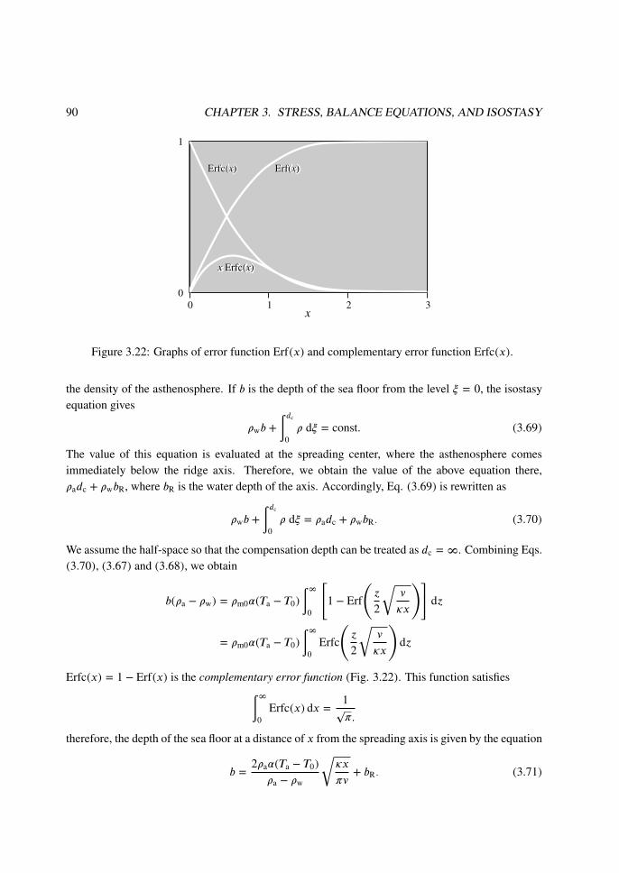
where Erf( ) is the error function (Fig. 3.22) defined by the equation

Erf(x) =2√π

∫x0

e−η2

dη (x ≥ 0). (3.66)

The graph of the error function designates that the shallow and deep parts of the suboceanic mantlehave steep and gentle geothermal gradients (Fig. 3.22). The turning point gradually goes downin the mantle with the denominator,

√κt, in the operand of the error function in Eq. (3.65). The

denominator has the dimensions of length so that√κt is called the diffusion length. Obviously, an

isotherm descends with age as ξ ∝ √κt.

The error function has an inverse function. Therefore, the depth of the isotherm with a specifictemperature T is given by Eq. (3.65), where the left-hand side is known. Substituting t = x/v andξ = x into the equation, we have

T − T0

Ta − T0= Erf

(z

2

√v

κx

). (3.67)

The thermal evolution has been investigated in the above argument. Now we can calculate thesubsidence. It is know that the density of rock at the temperature ΔT , which is measured from thereference temperature T0, changes as

ρ = ρ0(1 − αΔT ), (3.68)

where ρ0 is the density at the reference temperature and α is the thermal expansion coefficient. Rockshave a representative value for the coefficient at about 3 × 10−5 K−1. We use ρa = ρm0(1 − αTa) for


Figure 3.22: Graphs of error function Erf(x) and complementary error function Erfc(x).

the density of the asthenosphere. If b is the depth of the sea floor from the level ξ = 0, the isostasyequation gives

ρwb +∫ dc

0ρ dξ = const. (3.69)

The value of this equation is evaluated at the spreading center, where the asthenosphere comesimmediately below the ridge axis. Therefore, we obtain the value of the above equation there,ρadc + ρwbR, where bR is the water depth of the axis. Accordingly, Eq. (3.69) is rewritten as

ρwb +∫ dc

0ρ dξ = ρadc + ρwbR. (3.70)

We assume the half-space so that the compensation depth can be treated as dc = ∞. Combining Eqs.(3.70), (3.67) and (3.68), we obtain

b(ρa − ρw) = ρm0α(Ta − T0)∫∞

0

[1 − Erf

(z

2

√v

κx

)]dz

= ρm0α(Ta − T0)∫∞

0Erfc

(z

2

√v

κx

)dz

Erfc(x) = 1 − Erf(x) is the complementary error function (Fig. 3.22). This function satisfies∫∞0

Erfc(x) dx =1√π,

therefore, the depth of the sea floor at a distance of x from the spreading axis is given by the equation

b =2ρaα(Ta − T0)ρa − ρw

√κx

πv+ bR. (3.71)

3.13. HORIZONAL STRESS RESULTING FROM TOPOGRAPHY 91

The depth increases with the square root of the distance, as we have assumed a constant spreadingrate at the ridge center.

We are able to estimate the effective values for the thermal diffusivity and thermal expansioncoefficient of the oceanic mantle by comparing the above model with observations. However, it isimportant that old sea floors are shallower than the depth predicted by the model (Fig. 3.20) and theocean basins have different deviations. Some factors other than the cooling are responsible for thisflattening. It is pointed out that reheating by hotspots cannot account for the deviations [198].

3.13 Horizonal stress resulting from topography

Large-scale topographic undulation is one of the sources of tectonic stress. Ocean floors show thedifference in their depth up to a few kilometers (Fig. 3.20) so that great stress may be generated.Following Dahlen [47], let us consider how large is the stress level associated with the variation ofthe depth of the ocean floor. In conclusion, the ridge push is the force resulting from the topography.The force is important among other origins of tectonic stresses including the colliding force of plates.

The asthenosphere comes immediately below the spreading axis, therefore we assume a constantdensity ρ0 under the axis. The coordinatesO-xz shown in Fig. 3.21 are used in this section. Considerthe density distribution

ρ(x, z) = ρ0 + ρ(x, z),

where the last term is the density anomaly from the reference density ρ0. According to Eq. (3.65),the temperature and the resultant density anomalies were derived in the previous section as

T (z, t) = Ta Erf(

z

2√κt

),

∴ ρ(z, t) = ρm0αTa Erfc(

z

2√κt

). (3.72)

The force FR that a unit length of the ridge axis is determined by the dipole moment of verticaldensity distribution (§3.11). The moment is obtained from Eq. (3.72) so that

FR =∫∞

0ρgz dz =

(ρm0gαTaκ

)t.

Consequently, the force is proportional to the age of the oceanic lithosphere15. The constant ofproportionality is about 0.035 TNm−1/m.y. For example, the ocean floor with an age of 80 m.y.has FR = 2.8 TNm−1. The force resulting from the ocean-continent topographic contrast has amagnitude of about 1.6 TNm−1 (§3.11). Therefore, the ridge push is as great as the force by thecontrast.

15The integral is taken over the range [0, ∞]. However, the contribution from the asthenosphere is negligible because ofErfc(x) � 1 for x > 2 (Fig. 3.22).


In the above argument, we used the density profile under the spreading axis as the reference.It is the next problem where the proper area that provides the reference is sought. If the densitydistribution was under the summit of Mount Everest, the entire world would have been under acompressional stress field. However, this is not the case. Accordingly, Coblentz and others excludedthe arbitrariness in the choice of reference by taking global topography into account [42].

Let the levels of the top and base of the lithosphere be z = h and z = L, respectively. Notethat the vertial force per unit area is σzz × (1 m2) and that the product of force and length has thedimensions of energy. Then the quantity

U =∫Lh

σzz dz =∫Lh

∫ hξ

ρ(ξ)g dξdz

is the potential energy of the lithospheric column with the unit sectional area. A region with a largeU tends to be subject to extensional tectonics. That with a small U is ready to be horizontallycontracted. The global average is estimated at 2.4 TNm−1 [42]. The threshold altitude for thecontinent is ±200 m, and the threshold depth of the ocean is about 4.3 km. Spreading centers havedepths actually shallower than this threshold. However, the topography is not the only cause oflithospheric stress. Therefore, an extensional stress field rifts continents and eventually breaks upthe continental lithosphere.

3.14 Thermal subsidence of continental rifts

It was shown in the previous chapter that the subsidence history of a passive continental margin isrevealed from stratigraphic records. Here we consider Mckenzie’s simple stretching model to linkthe subsidence and rifting together.

Post-rift subsidence

Passive margin subsidence after continental breakup is generally associated with very weak or nofault activity. Extensional tectonics does not account for the subsidence. In contrast, the continentallithosphere is thinned and horizontally extended during the rift phase. The fact is that the riftingaccounts for the post-rift subsidence.

Consider the thermally equilibrium state of the lithosphere illustrated in Figs. 3.23(a) and (c),i.e., the temperature at the base of the lithosphere is Ta at a depth of z = tL. The temperaturedistribution before and long after rifting is assumed to be in equilibrium. The continental crust isthinned with the lithospheric mantle. The thinning of the crust results in subsidence. Let tc and tL bethe initial thickness of the crust and the lithosphere, respectively (Fig. 3.23(a)). It is also assumedthat the temperature at z = tL is kept at Ta. The top of the lithosphere was at sea level before rifting.

Here, the lithosphere is thought to be subject to homogeneous deformation in the rift phase. Ifthe lithosphere is horizontally extended by a factor of β, the thickness of the lithosphere and crustbecome tc/β and tL/β, respectively. The rift-stage subsidence is affected not only by the thinning

3.14. THERMAL SUBSIDENCE OF CONTINENTAL RIFTS 93

Figure 3.23: Diagrams showing the simple stretching model [138]. (a) Structure and temperaturedistribution in the lithosphere in the pre-rift stage, (b) at the end of rifting, and (c) in post-rift stage.

but also by the temporal variation of the thermal regime, because rock density changes with thevariation as

ρ = ρ0(1 − αT ), (3.73)

where ρ0 is the reference density at T = 0◦ C. If the thinning of the lithosphere is quick compared tothe time constant of heat conduction, isotherms in the lithosphere are uplifted adiabatically16 (Fig.3.23(b)). If we assume isostatic compensation throughout the rifting process, we obtain the syn-riftsubsidence

Si =tLρa − tcρc − (tL − tc)ρm

ρa − ρw

(1 − 1

β

), (3.74)

where ρc, ρm and ρa are the representative densities of the crust, mantle lithosphere, and astheno-sphere, respectively, and are given by

ρa = ρm0(1 − αTa), ρc = ρc0

(1 − αTa

2tctL

), ρm = ρm0

(1 − αTa

2− αTa

2tctL

).

16This assumption is valid for the rifting with a duration shorter than ∼25 m.y. [92].


Table 3.2: Parameters for the simple stretching model.

ρm0 = 3.3 × 103 kg m−3 α = 3.5×10−5 K−1 tL = 100 kmρc0 = 2.8 × 103 kg m−3 κ = 1.0×10−6 m2 s−1 tc = 35 kmρw = 1.0 × 103 kg m−3 Ta = 1333◦ C

The coefficients, ρc0 and ρm0 are the reference densities of the crust and mantle. Si is called theinitial subsidence in the passive margin formation. Substituting the representative densities into Eq.(3.74), we obtain the magnitude of the initial subsidence

Si = Si0

(1 − 1

β

), (3.75)

Si0 =

[(ρm0 − ρc0)

(1 − αTa

2tctL

)tctL

− ρm0αTa

2

]tL

ρm0(1 − αTa) − ρw. (3.76)

The latter quantity, (Si0) can have positive and negative signs depending on the initial thickness ofthe crust. Since the denominator in the right-hand side of Eq. (3.76) is positive, the sign depends onthe numerator. Solving the equation, (numerator) = 0, we obtain the solution,

tctL

=ρm0 − ρc0

α(ρm0 − ρc0)Ta±[4(ρm0 − ρc0)2 + 4α2(ρm0 − ρc0)ρm0T

2a

]α(ρm0 − ρc0)Ta

.

Using the parameters shown in Table 3.2, we obtain the ratio tc/tL = 0.154 and 42.7. However, thisratio should be less than unity so that the latter is a meaningless solution. The former indicates athreshold initial thickness of tc ≈ 15 km. The lithosphere with a continental crust initially thickerthan ∼15 km subsides through the lithospheric thinning, but the surface is uplifted by rifting if thecrust is initially thinner than this value. The uplift is due to a steepening of the geothermal gradient.That is, the attenuation of the lithospheric mantle plays an opposite role to that of the continentalcrust. Island arcs have volcanism so that their lithosphere is thinner than the ordinary continentallithosphere. If an island arc has a lithosphere with a pre-rift thickness of tL = 50 km, then the archas the threshold at about 7 km. The geohistory analysis of syn-rift sediments can constrain β withEq. (3.75). This parameter is called the stretching factor.

The thermal regime is altered by the rifting. Isotherms between 0◦ and Ta are raised by the rifting(Fig. 3.23(b)). After the rifting, the isostherms descend to the equilibrium level in the long run (Fig.3.23(c)). This post-rift cooling causes a gradual subsidence of the passive margin. This is called thethermal subsidence of the lithosphere. The simple stretching model (Fig. 3.23) allows us to estimatethe rate and amount of this subsidence [138].

In order to calculate the heat conduction after the termination of rifting, the initial subsidence isneglected because Si � tL. Therefore, the thermal conduction equation ∂T/∂t = κ∂2T/∂z2 is solvedwith the boundary condition T = 0 at z = 0. In addition, the temperature at z = tL is assumed to be

3.15. KINEMATIC MODEL OF SYN-RIFT SUBSIDENCE 95

kept at T = Ta. The time t is measured from the termination. The initial condition is shown by thegraph in Fig. 3.23(b), which is the temperature distribution at the end of rifting. Solving this system,we obtain the thermal evolution

T

Ta=

(1 − z

tL

)+

2π

∞∑n=1

(−1)n+1

n

β

nπsin

nπ

βsin

nπz

tLe−n

2t/τ , (3.77)

τ = π2t2L/κ. (3.78)

The parameters shown in Table 3.2 give the time constant τ = 3.2 m.y.Combining Eqs. (3.73) and (3.77), we obtain the evolution of the density structure ρ(z, t) .

Isostatic compensation through time is expressed as∫ tL0ρ(z, t) dz + ρwSt =

∫ tL0ρ(z, 0) dz,

where St is the thermal subsidence,

St ≈[

4αρm0TatL

π2(ρm0 − ρc0)

]β

πsin

π

β

(1 − e−t/τ

). (3.79)

Higher-order terms in Eq. (3.77) are neglected in deriving Eq. (3.79).Equation (3.79) shows that the rate of thermal subsidence decays as the exponential function.

The subsidence curve shown in Fig. 3.16 has this shape. Fitting the curve given by Eq. (3.79), weobtain the stretching factor for the area the curve was determined.

3.15 Kinematic model of syn-rift subsidence

Post-rift subsidence results from the cooling of the lithosphere, whereas syn-rift subsidence is con-trolled by not only the thermal but also the mechanical properties of the lithosphere. The latteraffects the characteristics of rift zones such as their widths and depths. Decompression melting ofthe asthenosphere under rift zones causes uplift through the buoyancy of magma. Therefore, theobservation of syn-rift subsidence sheds light on the deep seated factors and on the secular changesof these factors.

The simple stretching model (§3.14) assumed an instantaneous thinning of the lithosphere andneglected the details of the rifting processes. In this section, we consider a mathematical inversemethod to constrain the rift-phase strain rate of the lithosphere from an observed rift-phase subsi-dence curve (Fig. 3.24) [259].

Consider a pure shear rift with horizontal and vertical strain rates of Exx and Ezz, respectively.The lithosphere is extending horizontally so that we have Ezz < 0 < Exx. The pre-rift levels of thetop and base of the lithosphere is z = 0 and z = a. The lithosphere is subject to a pure shear, so thatwe have

−εzz = εxx = G(t),


where the function G(t) is defined to describe the temporal variation of the strain rates and is linkedto the rate of subsidence in the following discussion.

Consider that the horizontal velocity field is symmetric with respect to the plane x = 0. Thelithosphere is assumed to undergo homogeneous strain so that the horizontal velocity u(x, t) is pro-portional to x. That is, we have

u(x, t) = G(t) x. (3.80)

Syn-rift subsidence reaches several kilometers, but is negligible compared to the representativethickness of continental lithosphere. Therefore, we assume the top of the lithosphere is kept at z = 0during the calculation of the lithospheric strain. This assumption allows us to write the descendingvelocity of rocks at depth z as

v(x, t) = −G(t) z. (3.81)

Note that this is the velocity in the +z direction.Subsurface temperature distribution affects the subsidence of this rift. The thermal conduction

equation to be solved should include velocity, because heat is transported not only by conductionbut also by travelling rocks. Hence, the left-hand side of the thermal conduction equation, ∂T/∂t =κ∇2T , should be replaced by the material derivative (Eq. (2.20)). That is, the equation

∂T

∂t+

[∇ ·

(uv

)]T = κ

(∂2T

∂x2+∂2T

∂z2

)(3.82)

governs the thermal evolution. From Eqs. (3.81) and (3.80), we have[∇ ·

(uv

)]T = G(t)x

∂T

∂x− G(t)z

∂T

∂z. (3.83)

If there was no horizontal variation in the initial temperature distribution, the pure shear would notraise horizontal temperature variation. Therefore, we have

∂T

∂x=∂2T

∂x2= 0.

Combining this and Eqs. (3.82) and (3.83), we obtain

∂T

∂t+ Gz

∂T

∂z= κ

∂2T

∂z2. (3.84)

The boundary conditions that we assume for the temperature evolution are T = 0 at z = 0 andT = Ta at z = a. The initial condition and the equilibrium temperature distribution is the constantgeothermal gradient to a depth of z = a.

The subsidence of this rift is the sum of the subsidence due to the thinning of the lithosphereand to the thermal perturbation. The former is described by Eq. (3.75). The equation describing thelatter factor should have the form

Q(t) = B

∫ a0

[T (z, t) − T (z,∞)

]dz, (3.85)

3.15. KINEMATIC MODEL OF SYN-RIFT SUBSIDENCE 97

Figure 3.24: (a) Strain rate history of a Triassic rift in northern Italy determined from a subsidencecurve of the rift (b). The 95% confidence region is shown in (a) by white [259].

where B = αρm/(ρa − ρw) is the factor to account for the buoyancy of the crust. Therefore, we havethe total subsidence

S(t) = A

(1 − 1

β

)− BQ(t), (3.86)

where A = tc(ρm − ρc)/(ρa − ρw). Crustal thinning has a positive effect for the total subsidence, butthe thinning of the lithosphere increases the geothermal gradient which has a negative effect for thesubsidence. Rearranging Eq. (3.86), we have

β =A

A − S − BQ(t). (3.87)

Equation (2.39) links the stretching factor β and G(t) as

β = exp[∫ tR

0G(t) dt

], (3.88)

where tR is the time ellapsed since the rifting began. Accordingly, combining Eqs. (3.87) and (3.88),we obtain the strain-rate history of the rift

G(t) =ddt

{ln[

A

A − S(t) − BQ(t)

]}. (3.89)

The rift-phase strain-rate history can be evaluated from observations for a pure shear rift. Theright-hand side of Eq. (3.89) has S(t) that is determined from the quantitative stratigraphy of therift. However,Q(t) depends on the unknown G(t) through Eq. (3.84). Therefore, G(t) is determinedby a mathematical inversion17 from the observed subsidence history S(t). Figure 3.24(a) shows the

17See [259] for detail.


optimal strain-rate history for the subsidence history of a Triassic rift zone in northern Italy (Fig.3.24(b)). The subsidence curve of the Triassic rift has an inflection point at about 220 Ma (Fig.3.24(b)). After the point, the subsidence curve is similar to an exponential curve, suggesting thermalsubsidence. The point designates a rejuvenated rifting, and corresponding to the second peak in thestrain-rate history.

A sharp decline in the strain rate by several orders of magnitude indicates the termination of rift-ing; the rift was aborted or the area became a passive margin. Timing of the termination determinedby the inverse method for the Triassic rift has a large uncertainty which is illustrated by the 90%confidence region between 100 and 220 Ma in Fig. 3.24(a). The umbiguity stems from the difficultyto detect very slow rifting if it overlaps simultaneous thermal subsidence. More definite constrainscome from geological structures. The termination of rifting is marked by the cessation or distinctdecline of fault activity. For example, the cross-section in Fig. 3.12 shows that the subsidence ofwedge shaped grabens had ceased by the early Jurassic. If rifting was successful to form a passivecontinental margin, the magnetic anomaly near the continent-ocean boundary provides a constraintfor the timing. Some passive margins were remarkably uplifted when continents were broken off themargins. Such a unconformity is known as a breakup unconformity [59].

3.16 Exercises

3.1 Assume a state of stress with the principal stresses σ1 = 4 MPa, σ2 = 5 MPa and σ3 = 8 MPa,and vertical σ1-axis and horizontal σ3-axis oriented due east. Determine the magnitude of the normaland shear stresses acting on the block beneath a fracture plane of which trend and dip are N030◦Eand 60◦SE, respectively. How much is the rake of the maximum shear stress on the plane?

3.2 Explain qualitatively why the function g(r) shown in Fig. 3.7(b) is convex downward and whythe function decreases with increasing r in the lower mantle.

3.3 What is the magnitude of the lithostatic pressure at the Moho interface. Assume the thicknessand density of the crust at 35 km and 2.8 × 103 kg m−3, respectively.

3.4 Derive Eq. (3.46).

3.5 Estimate how much is the force per unit boundary length with which the Tibetan Plateau pushesthe Hindustan Plain due solely to the structure illustrated in Fig. 3.25.

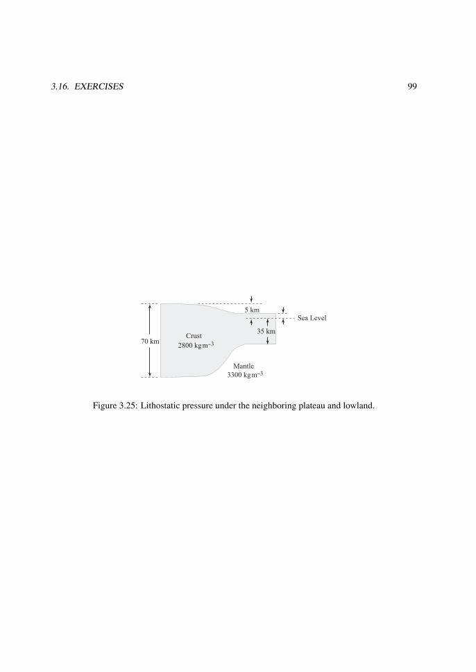
3.16. EXERCISES 99

Figure 3.25: Lithostatic pressure under the neighboring plateau and lowland.

Documents

Stress, Balance Equations, and Isostasy - · PDF fileStress, Balance Equations, and Isostasy We deﬁne stress to consider forces acting at depths, and derive the equations of mass,