Preprints of theMax Planck Institute for

Research on Collective GoodsBonn 2015/9

Strategic Disclosure of Demand Information by Duopolists: Theory and Experiment

Jos Jansen Andreas Pollak

MAX PLANCK SOCIETY

Preprints of the Max Planck Institute for Research on Collective Goods Bonn 2015/9

Strategic Disclosure of Demand Information byDuopolists: Theory and Experiment

Jos Jansen / Andreas Pollak

July 2015

Max Planck Institute for Research on Collective Goods, Kurt-Schumacher-Str. 10, D-53113 Bonn http://www.coll.mpg.de

Strategic Disclosure of Demand Information by

Duopolists: Theory and Experiment∗

Jos Jansen

Aarhus University†

Max Planck Institute, Bonn

Andreas Pollak

University of Cologne‡

July 2015

Abstract

We study the strategic disclosure of demand information and

product-market strategies of duopolists. In a setting where both

firms receive information with some probability, we show that firms

selectively disclose information in equilibrium in order to influence

their competitor’s product-market strategy. Subsequently, we ana-

lyze the firms’ behavior in a laboratory experiment. We find that

subjects often use selective disclosure strategies, and this finding ap-

pears to be robust to changes in the information structure, the mode

of competition, and the degree of product differentiation. Moreover,

in our experiment, subjects’ product-market conduct is largely con-

sistent with theoretical predictions.

Keywords: duopoly, Cournot competition, Bertrand competition, information dis-

closure, incomplete information, common value, product differentiation, asymmetry,

skewed distribution, laboratory experiment

JEL Codes: C92, D22, D82, D83, L13, M4

∗We thank Axel Ockenfels for essential advice on experimental design, and for continuous guid-ance. We also thank Patrick Bolton, Christoph Engel, Yvonne Giesing, Kenan Kalayci, Armando

Pires, Bettina Rockenbach, Jean-Philippe Tropeano, Peter Werner, and the participants of the MPI

Workshop (Bonn), EARIE conference (Rome), NORIO (Oslo), IO Workshop (Alberobello), Nordic

Conference on Behavioral and Experimental Economics (Aarhus), SMYE (Ghent), and seminar audi-

ences at the Catholic University in Milan, University of Cologne, and Aarhus University for valuable

comments. We gratefully acknowledge the research support from the team at the chair of Prof.

Ockenfels, and financial support from the Deutsche Forschungsgemeinschaft for the experiments and

laboratory. Jansen gratefully acknowledges the support of the WZB (Berlin) and University of Surrey

where part of the research for this paper was done. Naturally, all errors are ours.†Corresponding author. Address: Dept. of Economics and Business Economics, Aarhus Univer-

sity, Fuglesangs Allé 4 (Building 2632/L), DK-8210 Aarhus V, Denmark; E-mail: jjansen@econ.au.dk‡Address: Department of Economics, Chair Prof. Axel Ockenfels, University of Cologne, Albertus-

Magnus-Platz, D-50923 Cologne, Germany; E-mail: pollak@wiso.uni-koeln.de

1 Introduction

This paper studies strategies of firms that may not have complete information about

the demand for their goods. The market demandmay be affected by exogenous shocks,

such as the business cycle or the weather. For example, a firm may not know whether

its market demand remains depressed (booming) or a recovery (recession) is imminent.

In addition, the firm may not be fully informed about how well product characteristics

match with consumers’ tastes if those tastes are subject to change. Alternatively,

a firm may not have complete information on a common cost of production. For

example, prices of common inputs may fluctuate in an unpredictable way. In all those

cases, a firm can obtain information to learn about the market, and if it does, it

can use this information to gain a strategic advantage. First, the firm can manage

the beliefs of a competitor by disclosing or concealing its information. Second, the

firm can use the information to make better-informed choices in the product market.

In this paper, we study these strategic uses of a firm’s demand information both

theoretically as well as experimentally.

The analysis of the firms’ disclosure incentives is relevant as starting point for

developing antitrust policy and accounting rules. An antitrust authority is better

equipped to determine how much information firms should be allowed to share, by

understanding the non-cooperative disclosure strategies of competing duopolists (e.g.,

Kühn and Vives, 1995, and Kühn, 2001). Likewise, it is helpful to know how much

information firms share voluntarily when one designs accounting rules that stipulate

how much information firms are required to disclose (e.g., Verrecchia, 2001, and Dye,

2001). In other words, the effects of disclosure regulation can only be properly as-

sessed if the unregulated disclosure strategies and their effects on product-market

competition are well understood.

If there are no verification and disclosure costs, and if it is known that firms have

information, then often firms will disclose all information. Firms do so, since they

cannot credibly conceal unfavorable news. This phenomenon is called the unraveling

result (Milgrom, 1981, Milgrom and Roberts, 1986, Okuno-Fujiwara et al., 1990, and

Milgrom, 2008).1 In the experimental literature, King and Wallin (1991a), and Jin et

al. (2015) find support for the unraveling result if receivers get enough feedback.

By contrast, if a firm can fail to become informed, it is no longer known whether

this firm is informed. Although information is verifiable, it is not verifiable whether or

1The assumption that information is verifiable, which we adopt in this paper, is consistent with

some empirical findings (e.g., see Jansen, 2008).

1

not a firm is informed. In such an environment the unraveling result may fail to hold

since firms can credibly conceal unfavorable news by claiming to be uninformed, e.g.,

see Dye (1985), Farrell (1986), Jung and Kwon (1988), and Sankar (1995). In these

models of unilateral disclosure, a Cournot oligopolist has an incentive to disclose

bad news (low demand), and conceal good news (high demand) to discourage its

rivals. A Bertrand oligopolist only discloses good news (high demand) to induce the

competitors to choose high prices. Ackert et al. (2000) give experimental support for

unilateral, selective information disclosure of a common cost parameter in Cournot

duopoly. They confirm that a firm discloses bad news more often than good news.2

Theoretical studies of multilateral information disclosure typically focus on sym-

metric models.3 Darrough (1993) analyzes a symmetric model, and Jansen (2008)

focuses on symmetric equilibria. These papers show that the optimal unilateral dis-

closure strategy is also an equilibrium strategy in symmetric settings of multilateral

disclosure. That is, symmetric Cournot duopolists disclose low demand intercepts and

conceal high intercepts, whereas Bertrand duopolists disclose only high intercepts. As

far as we know, there are no experiments on multilateral disclosure in duopoly models.

Although the literature focuses on unilateral disclosure and multilateral informa-

tion exchange between symmetric firms, there exist important differences between

firms in practice (e.g., established firms differ from new firms, and firms have different

sizes and capabilities). Our paper intends to address this issue.

We contribute to the literature in two ways. First, we contribute to the theoret-

ical literature on multilateral information disclosure by analyzing the disclosure and

product-market strategies of firms in asymmetric duopolies. Second, we contribute

to experimental work on strategic information disclosure by studying multilateral dis-

closure, by analyzing the behavior of Bertrand duopolists, and by studying disclosure

behavior of duopolists with differentiated goods in a laboratory.

A firm’s disclosure of common demand information in a Cournot duopoly has

two conflicting effects. First, the disclosure informs the firm’s competitor about his

payoff from the product market. In particular, if the firm discloses that demand is low

(high), then its competitor learns that a relatively low (high) output level is profitable.

Therefore, this effect gives the firm an incentive to disclose a low demand intercept

and conceal a high intercept in order to discourage supply by its competitor.

However, there is an additional effect of demand disclosure. A firm that discloses

2King and Wallin (1991b) obtain results consistent with selective disclosure in an asset market.

In a labor market, costly disclosure to an automated receiver is selective too (Benndorf et al., 2015).3With multilateral disclosure, both firms in a duopoly make (simultaneous) disclosure choices.

2

information also informs its competitor about its conduct in the product market. In

particular, if the firm discloses that it learned that demand is low (high), then it

signals to the competitor that it will have a less (more) “aggressive” output strategy

than an uninformed firm. This effect gives the firm an incentive to disclose a high

demand intercept and conceal a low demand intercept. Such a disclosure strategy

makes the firm’s competitor pessimistic about the competitive pressure, and thereby

discourages him to supply to the market (strategic substitutes).

Our paper derives precise conditions under which the former effect outweighs the

latter. In particular, if the demand distribution is not too skewed towards low demand,

or if firms do not differ too much from each other, then there exists an equilibrium in

which both firms disclose low demand and conceal high demand. Hence, we extend

the aforementioned literature by allowing for asymmetry and multilateral disclosure.

In addition, we characterize situations where the latter effect of disclosure domi-

nates the former, and a firm reverses its disclosure strategy. This happens if demand is

sufficiently skewed towards low demand (e.g., in periods of economic recession), and if

one firm is likely to be informed while the other firm is unlikely to be informed. In this

case, the former firm discloses only a low intercept whereas the latter firm discloses

only a high demand intercept. If it is unlikely that a firm is informed and it is likely

that the demand is low, then this firm is expected to be a soft competitor, since it

is likely that the firm is uninformed and pessimistic. Disclosure of good news by this

firm makes the competitor less “aggressive,” since the news makes the competitor re-

alize that the firm will be less soft than expected.4 Hence, if the firms’ probabilities of

receiving information are sufficiently different, then the firms’ information disclosure

choices may differ from the choices by identical firms.5

In a Bertrand duopoly, the effects from disclosing information about a common

demand intercept are aligned. As before, the disclosure of high (low) demand informa-

tion makes the competitor of a firm optimistic (pessimistic) about his product-market

opportunities. In addition, the firm’s disclosure of a high (low) demand intercept

signals to the firm’s competitor that it will have a less (more) “aggressive” pricing

strategy than if it were uninformed. Both belief updates give the competitor the in-

4This happens for the following reasons. First, the competitor drastically updates his belief about

the firm’s conduct in the product market, and thereby expects fiercer competition. Moreover, the

average competitor becomes only slightly more optimistic about his own opportunities in the product

market, since it is very likely that the competitor was already informed about the size of the market.5This observation is consistent with the observations in Hwang (1993, 1994). Hwang analyzes

the information sharing incentives of precommitting firms (Kühn and Vives, 1995, Raith, 1996, and

Vives, 1999), whereas we study the incentives for strategic disclosure.

3

centive to set a relatively high (low) price. Therefore, the firm discloses a high demand

intercept and conceals a low intercept to encourage a high price by its competitor.

Our laboratory experiment analyzes the strategic information disclosure and prod-

uct market choices of firms in several duopolistic settings. In particular, we vary

the mode of competition, the information structure (i.e., from unilateral to bilateral

disclosure, and from symmetric to asymmetric models), and the degree of product

differentiation across seven treatments.

We find that subjects often use selective disclosure strategies. The subjects in our

treatments with Cournot (Bertrand) competition disclose information on low (high)

demand intercepts significantly more often than information on high (low) demand in-

tercepts. These observed tendencies suggests that subjects understand that disclosed

information informs their competitor about demand, and they use their information

strategically. The observed selective disclosure strategies give the subjects’ competitor

pessimistic (optimistic) beliefs about the market with Cournot (Bertrand) competi-

tion, and thereby make the competitor less “aggressive” in the product market if this

were the only effect of information disclosure. Our finding appears to be robust to

changes in the information structure, and the degree of product differentiation.

Finally, the subjects in our experiment display product-market conduct that is

largely consistent with our theoretical predictions. Their product-market choices tend

to be responsive to information, and (weakly) to the precision of information.

The paper is organized as follows. Section 2 describes the model. Section 3 derives

the equilibrium strategies of firms, and states experimental hypotheses. Section 4

describes the design of our experiment, and it discusses the experimental results.

Finally, Section 5 concludes the paper. The proofs of the paper’s theoretical results,

our test results, and the experiment’s instructions are relegated to the Appendix.

2 The Model

Consider an industry where two risk-neutral firms interact in a three-stage game.

Firms have symmetric demand functions, with intercept . This demand intercept

is unknown to the firms.6 The intercept is either low or high, i.e., ∈ { } with0 , and is drawn with probability () where 0 () 1 and ()+() = 1.

In stage 1, the firms can learn the demand realization from imperfect signals,

(Θ1Θ2). With probability , firm learns the true demand intercept, Θ = , but

6This model is conceptually identical to a model with incomplete information about a common

shock to a constant marginal production costs. Hence, all results hold for such a model as well.

4

with probability 1 − the firm receives the uninformative signal Θ = ∅, where0 1 and = 1 2. These signals are independent, conditional on .

In stage 2, each firm chooses whether to disclose or conceal its signal. If a firm

receives information about the demand intercept, then this information is verifiable.

However, the fact whether or not a firm is informed is not verifiable. If firm receives

information Θ = , it chooses the probability with which it discloses this information,

() ∈ [0 1] for = 1 2. In particular, firm discloses with probability (), while it

sends uninformative message ∅ with probability 1−() for = 1 2. An uninformed

firm can only send message ∅. In other words,£() ()

¤denotes firm ’s disclosure

strategy for = 1 2. Firms choose their disclosure strategies simultaneously.

In the final stage, firms simultaneously choose their output levels of substitutable

goods, ≥ 0 for firm (i.e., Cournot competition).7 Firm ’s inverse demand function

is P ( ) ≡ − − , for ∈ {1 2} with 6= , and 0 ≤ 1. Parameter

stands for the degree of product substitutability.8 Firm has the constant unit

cost of production ≥ 0. We assume that the firms’ costs do not differ too much,and thereby we focus on accommodating output strategies. Firm ’s profit for output

levels ( ) and demand intercept is (for ∈ {1 2} with 6= ):

( ; ) = ( − − − ), (1)

We solve the model backwards and use the perfect Bayesian equilibrium concept.

3 Theoretical Analysis

This section analyzes the equilibrium quantities for given disclosure choices, and char-

acterizes the equilibrium disclosure strategies. In addition, we characterize the equi-

librium strategies of Bertrand competitors. These analyses yield testable hypotheses.

3.1 Equilibrium Outputs

First, we study the equilibrium outputs under complete information. Whenever one

of the firms discloses the information , both firms know that the demand intercept

is . Firm ’s first-order condition of profit maximization with respect to , given

∈ { }, is as follows (for = 1 2 and 6= ):

2() = − − () (2)

7In Section 3.3, we extend the model by considering price competition (i.e., Bertrand competition).8For example, if = 1 then the firms’ goods are perfect substitutes, and if → 0 then in the limit

the firms supply to independent markets.

5

The first-order conditions give the following equilibrium output and profit for firm :

() = − 2 +

+( − )

4− 2and (3)

() = ()2, (4)

respectively, with ∈ { } and ∈ {1 2} with 6= . This is a standard result.

Second, we consider the equilibrium after no firm disclosed any information. In

that case, an informed firm with Θ = assigns probability (; ) to competing

with an informed rival (Θ = ), and probability 1−(; ) to facing an uninformed

rival (Θ = ∅), where:

(; ) ≡ [1− ()]

1− () (5)

After an uninformative signal (Θ = ∅), firm expects the demand intercept:

{|∅; } ≡ (; ) +(; ) (6)

with posterior belief

(; ) ≡ () [1− ()]

() [1− ()] + ()£1− ()

¤ (7)

The uninformed firm assigns probability (; )(; ) to competing with an

informed firm with Θ = for ∈ { }. With the remaining probability, 1 −{(; )|∅; }, firm is believed to be uninformed. Hence, if the beliefs of firm

are consistent with disclosure strategy , then firm ’s first-order conditions are as

follows (for = 1 2 with 6= , and Θ ∈ { ∅} where {|; } = ):

2∗ (Θ) = {|Θ; }−−

©(; )

∗() + [1−(; )]

∗(∅)

¯̄Θ;

ª (8)

Equation (8) implies that the equilibrium output of an uninformed firm equals the

conditionally expected output of an informed firm:

∗ (∅; ) = {∗ (; )|∅; } (9)

After we define the function D as follows

D( ) ≡ 4− 2£(; )(; ) +(; )(; )

¤∗ £(; )(; ) +(; )(; )

¤ (10)

we derive the equilibrium output from (8) and (9), by using (5)-(7).

6

Proposition 1 If no firm disclosed information, and firms and have beliefs con-

sistent with and , respectively, then the following holds for = 1 2 with 6= .

The equilibrium output of firm with information Θ = equals:

∗ (; ) ≡ () +

4−2 (

b)³ − b´( )

D( )Q2

=1 [1− ()]{1− ()}(11)

where

( ) ≡ (1− )(1− ) {[1− ()] [1− ()]}+2(1− ) [1− ()]

£1− ()

¤{1− ()}

−(1− ) [1− ()]£1− ()

¤{1− ()} (12)

and D( ) 0 for b ∈ { } with 6= b. In equilibrium, firm with signal

Θ ∈ { ∅} expects to earn the profit ∗ (Θ; ) ≡ ∗ (Θ; )2.

The sign of³b −

´· ( ) determines the sign of

() − ∗ (; ), since

all other terms are positive for = 1 2. This observation is important for the firm’s

incentive to disclose information, which we analyze in the next subsection.

3.2 Equilibrium Disclosure Strategies

Now we analyze the firms’ incentives to strategically disclose information. That is,

we look for strategies (∗ ∗) that are optimal given beliefs consistent with (

∗

∗).

Suppose that firm ’s beliefs are consistent with strategy ∗ , and firm has beliefs

that are consistent with ∗ . Given these beliefs, the expected profit of firm with

Θ = from disclosure probability () equals:

Π( ; ∗

∗) = () + [1− ()]

£1−

∗()

¤ ³∗ (;

∗

∗)− ()

´ (13)

Hence, the sign of firm ’s marginal expected profit from changing () depends on

the sign of the profit difference () − ∗ (; ∗

∗). In turn, the sign of the output

difference ()−∗ (; ) determines the sign of this profit difference, and therebythe incentive of firm to disclose information .

We illustrate the firms’ disclosure incentives in two extreme information-disclosure

constellations. First, we consider full disclosure (i.e., () = () = 1 for = 1 2).

Firm has the incentive to unilaterally deviate from full disclosure by concealing high-

demand information. Such concealment reduces the competitor’s output from ()

7

to { ()} if the competitor is uninformed, whereas it does not affect an informedcompetitor. The competitor’s output reduction is profitable for firm .

Second, we consider full concealment (i.e., () = () = 0 for = 1 2). With

prior beliefs and ex ante symmetric firms (i.e., = ), a firm has the incentive to

unilaterally deviate from full concealment by disclosing a low demand intercept.9 This

relaxes competitive pressure from the competitor, and increases the disclosing firm’s

profit. By contrast, if the firms are asymmetric, i.e., is low and is high, firm

may want to deviate by disclosing a high demand intercept.10 Yet, firm has the

incentive to unilaterally deviate from full concealment by disclosing a low intercept.11

These examples suggest that there is always a firm with an incentive to disclose

only low demand information. This disclosure incentive is also present in equilibrium.

Proposition 2 For any equilibrium, there exists a firm, , such that this firm chooses

the disclosure strategy£() ()

¤= (1 0).

Hence, it is without loss of generality to restrict attention to equilibria in which

one of the firms discloses only a low demand intercept. This simplifies the equilibrium

analysis, and it yields the following characterization.

Proposition 3 (a) There exists an equilibrium with symmetric disclosure choices

(i.e.,£∗ ()

∗ ()

¤= (1 0) for = 1 2) if and only if () [2 + (1− )] ≤ 2 for

= 1 2 with 6= ;

(b) For some = 1 2 with 6= , there exists an equilibrium with£∗ ()

∗ ()

¤=

(0 1) if and only if ()(2 + ) ≥ 2;(c) For some = 1 2 with 6= , there exists an equilibrium with 0 ≤ ∗ () ≤ 1 and

∗ () =1

µ1− (1− )()

2 [1− ()]

¶(14)

if and only if 2(2 + ) ≤ () ≤ 2 [2 + (1− )].

(d) No other equilibrium exists.

9It follows from (12) that ([0 0] [0 0]) = 2(1− )− (1− ) which is positive if = .10For example, if = , is close to 1, and is close to 0 (and both firms conceal all information),

then firm expects an output close to { ()} from firm . In turn, firm expects that firm is informed and will set its output approximately according to the best reply () = [ − −{ ()}]2. This output is higher than the output which firm sets after disclosure of high

demand information by firm (i.e., ()). In other words, the unilateral disclosure of Θ = allowsfirm to set a higher output, and thereby to reach a higher profit level.11Subsequently, firm supplies the output () instead of the higher output { ()}.

8

Proposition 2 implies that the equilibrium of Proposition 3(a) is the only symmetric

disclosure equilibrium that can exist. In this equilibrium, the incentive to make a

competitor pessimistic about the size of the market dominates. Proposition 3(a) gives

two conditions for the existence of this equilibrium. In particular, the conditions hold

if the distribution is not too skewed towards a low demand intercept (e.g., () ≤ 23).12

Alternatively, if firms are symmetric (i.e., = ), then Proposition 3(a) applies

too.13 Finally, product differentiation is favorable for the existence of the symmetric

disclosure equilibrium. In particular, there exists a critical degree of substitutability,

∗ 0, such that the conditions of Proposition 3(a) are satisfied for all ≤ ∗.14

Conversely, the proposition shows that the equilibrium with symmetric disclosure

choices need not always exist. In particular, if (i) the distribution of is skewed

towards low intercepts (i.e., () is high), (ii) goods are close substitutes (i.e., is

high), and (iii) it is very likely that one of the firms receives information while it is

unlikely that the other firm receives information (e.g., is high while is low), then

the symmetric disclosure equilibrium does not exist. Under those conditions, firm

has an incentive to unilaterally disclose good (conceal bad) news to make its rival

realize (believe) that firm will compete “aggressively” in the product market.

For intuition of these observations, suppose that the firms have beliefs consistent

with the strategies£∗ ()

∗ ()

¤=£∗()

∗()

¤= (1 0), and firm chooses the

strategy£∗()

∗()

¤= (1 0). It is convenient to consider the extreme situation

where () = 1 − , and = , = 1 − , with 0 small. In this situation, an

uninformed firm would expect a demand intercept of approximately 12

¡ +

¢, and

the firm would consider it approximately equally likely to compete with an informed

rival (Θ = ) as with an uninformed rival (Θ = ∅).15 Consequently, an uninformedfirm would supply approximately the amount

¡12

¡ +

¢¢.16

First, we consider the incentive for firm with Θ = to unilaterally deviate by

12In the rewritten condition () ≤ 2 ( [2 + (1− )]), the right-hand side is decreasing in and , and increasing in . This implies that 2 ( [2 + (1− )]) 23.13For = = , the conditions reduce to () [2 + (1− )] ≤ 2. This condition holds, since

its left-hand side is increasing in for 0 1 and therefore () [2 + (1− )] 2() 2.14The condition’s left-hand side is increasing in , and it is smaller than 2 for = 0.15This is due to the fact that both and () are high. In particular, the posterior probability

(; 1 0) in (7) equals 1(2− ), and (; 1 0) in (5) gives (; 1 0) = 0 and (; 1 0) = 1− .Clearly, for → 0, these probabilities converge to (; 1 0)→ 12 and (; 1 0)(; 1 0)→ 12.16An informed rival would know that the intercept is , whereas an uninformed rival would expect

approximately the low intercept , since () is high and the concealment by firm generates almostno additional information ( is low). Approximately, this gives the best reply functions: 2() ≈−−(∅) and 2(∅) ≈ −−(∅) for firm , and 2(∅) ≈ (+)2−−

£() + (∅)

¤2

for firm . Solving this system of equations gives ∗ (∅; ∗ ∗ ) ≈ (12

¡ +

¢) for firm .

9

disclosing a high demand intercept. If firm were to conceal its information, then

firm would expect to compete almost surely with an uninformed rival (since is

small), who supplies ¡12

¡ +

¢¢units. By contrast, the disclosure of the high

demand intercept makes firm realize that it faces a strong competitor, who sets the

output (). Clearly, firm ’s expected output from disclosure is greater than the

expected output from concealment, i.e., () ¡12

¡ +

¢¢. Now, irrespective

of whether firm discloses or conceals, the competitor’s best reply is approximately

2 ≈ − − , since it is extremely likely that firm is informed in the latter case

(i.e., is big). Whereas disclosure does not greatly affect firm ’s beliefs about the

demand, it has a substantial effect on firm ’s beliefs about firm ’s product market

conduct. This gives firm an incentive to contract its output. Hence, the unilateral

disclosure of Θ = is profitable for firm , given the proposed equilibrium beliefs.

Under the same conditions, firm with bad signal Θ = has the incentive to

conceal bad news. Here, firm ’s strategy can only have an effect on the firms’ product-

market conduct, if firm is uninformed. In this case, a similar intuition applies as

before. Although firm ’s strategy has a negligible effect on firm ’s beliefs about de-

mand, it has a substantial effect on the firm’s beliefs about the competitive pressure

from firm .17 Concealment makes uninformed firm expect fierce quantity competi-

tion, and firm reduces its output as a consequence. Firm ’s lower output enables

firm to expand its output, and thereby increase its expected profit.

Proposition 3(b) shows that the deviation strategies from above can be equilibrium

strategies. An asymmetric equilibrium can only exist if the intercept distribution is

skewed towards the low demand (i.e., () 2(2 + ) is a necessary condition).

Finally, Proposition 3(c) shows that there can exist equilibria in mixed strategies.

As in part (b), an equilibrium in mixed strategies can only exist if the distribution of

is skewed towards low intercepts (i.e., () 2(2+ )). Moreover, Proposition 3(c)

implies that an equilibrium with full disclosure or full concealment by firm only exists

in special cases (respectively, if () = 2(2 + ) or () = 2 [2 + (1− )]).

Proposition 3 has the following implication for the uniqueness of an equilibrium.

17With or without disclosure by firm , the competitor’s best reply is approximately 2 ≈ −−. This is due to the fact that is low and () is high. In particular, the posterior probability(; 1 0) in (7) equals

£(1− )2 +

¤, and (; 1 0) in (5) gives (; 1 0) = 0 and (; 1 0) = .

Clearly, for → 0, these probabilities converge to (; 1 0) → 0 and (; 1 0)(; 1 0) → 0.

Whereas firm anticipates the competitor’s output () after disclosure, it expects approximately

the output ¡12

¡ +

¢¢after concealment.

10

Corollary 1 (a) For ()max{1 2} 2(2 + ), the firms choose symmetric dis-

closure strategies (i.e.,£∗ ()

∗ ()

¤= (1 0) for = 1 2) in the unique equilibrium.

(b) For () 2(2+) and () 2 [2 + (1− )] where = 1 2 with 6= ,

the firms choose the strategies£∗ ()

∗ ()

¤= (0 1) and

£∗()

∗()

¤= (1 0) in the

unique equilibrium.

Corollary 1(a) confirms the result of Darrough (1993). For the symmetric distri-

bution (i.e., () = 12) and symmetric probabilities of receiving an informative signal

( = ), the symmetric equilibrium is unique. In our setting with a binary type

space, symmetry of the distribution is already sufficient for uniqueness.

In the setting where only one firm can become informed, we confirm Sankar (1995).

Corollary 2 (Sankar, 1995) If = 0, then firm chooses strategy£() ()

¤=

(1 0) in the unique equilibrium for = 1 2 with 6= .18

In the context of a model with a symmetric distribution, Sankar (1995) argues

that this result extends to settings with 0. Our contribution is to show that

this argument depends on the symmetry of the distribution. In particular, if the

distribution is sufficiently skewed towards a low intercept, then the equilibrium with

symmetric disclosure choices may not be unique or may not exist (Corollary 1(b)).

3.3 Bertrand Competition

This subsection analyzes the incentives of firms that compete in prices. Inverting the

system of inverse demand functions gives the following direct demand function:

( ; ) ≡ 1

1− 2

µ(1− ) + −

¶(15)

for = 1 2with 6= . Maximizing the expected value of profit = ( − )( ; )

and solving for the equilibrium gives the following result by focusing on accommodat-

ing pricing strategies (i.e., the substitutability parameter is sufficiently low).

Proposition 4 If a firm disclosed , then firm sets the equilibrium price:

() ≡(1− ) +

2− +

( − )

4− 2 (16)

18Corollary 2 follows from the fact that (12) reduces to () = 2 [1− ()]£1− ()

¤ 0

for = 0. Consequently, there only exists an equilibrium with£() ()

¤= (1 0).

11

If no firm disclosed information, and firms and have beliefs consistent with and

, respectively, then the equilibrium price of firm with information Θ = equals:

∗ (; ) ≡ ()− 1−2−(

b)³ − b´( )

D( )Q2

=1 [1− ()]{1− ()}(17)

where (•) 0 and D(•) 0 for b ∈ { } with 6= b, and = 1 2

with 6= . The equilibrium price of an uninformed firm equals ∗ (∅; ) = {∗ (; )|∅; } for = 1 2 with 6= . Firm chooses the strategy

£() ()

¤=

(0 1) in the unique equilibrium for = 1 2.

The intuition for this result is straightforward. The effects of information dis-

closure by Bertrand competitors reinforce each other, whereas demand disclosure by

a Cournot competitor yields two conflicting effects. Disclosure of good news about

the market size increases the competitor’s price for two reasons. First, the competi-

tor becomes more optimistic about the market opportunities (i.e., the demand), and

raises its price. In addition, the competitor learns that the disclosing firm is informed

about the fact that demand is high, and is therefore less “aggressive” than expected.

Also this makes the competitor a softer price setter in the product market (strategic

complements). The intuition for concealing bad news is analogous.

3.4 Hypotheses

Our theoretical results yield some hypotheses which we test afterwards. First, we

derive the following testable hypothesis from Corollary 1 and Proposition 4.

Hypothesis 1 (a) If demand is uniformly distributed (() = 12) and firms compete

in quantities (prices), then firms disclose information on low (high) demand intercepts

more often than high (low) intercepts.

(b) If firms compete in quantities and the conditions of Corollary 1(b) are satisfied,then firm (firm ) discloses information on high (low) demand intercepts more often

than low (high) intercepts.

Hypothesis 1(a) gives testable predictions for settings in which firms choose sym-

metric disclosure strategies in the unique equilibrium. Hypothesis 1(b) covers the

settings in which the disclosure strategies differ in the unique equilibrium.

Second, we develop two testable hypotheses about the effects of information on

the firms’ product-market strategies.19 If firms compete in quantities and the demand

19See the Supplementary Appendix for details on formal derivations.

12

distribution is uniform (i.e., () = 12), then firms choose the disclosure strategy

1 = 2 = [1 0] in the unique equilibrium (Proposition 3), and Proposition 1 gives:

∗ (; [1 0] [1 0]) () ∗ (∅; [1 0] [1 0]) () ∗ (; [1 0] [1 0]) (18)

for = 1 2. A firm’s incentive to conceal follows from the last inequality of (18).

By contrast, under the conditions of Corollary 1(b), firm discloses only high demand

intercepts in the unique equilibrium, and its equilibrium outputs compare as follows:

() ∗ (; [0 1] [1 0]) ∗ (∅; [0 1] [1 0]) ∗ (; [0 1] [1 0]) () (19)

Firm ’s incentive to conceal follows from the first inequality in (19). Similarly, if

firms compete in prices, then Proposition 4 shows that both firms disclose only high

demand intercepts in the unique equilibrium (i.e., 1 = 2 = [0 1]), and prices can be

ranked as follows (for = 1 2):

() ∗ (; [0 1] [0 1]) ∗ (∅; [0 1] [0 1]) ∗ (; [0 1] [0 1]) () (20)

Firm ’s incentive to conceal a low demand intercept follows from the first inequality

in (20). We summarize these observations in the following hypothesis.

Hypothesis 2 Consider firm with an informative signal (Θ = ).

(a) If demand is high ( = ) and it is drawn from the uniform distribution (() = 12),

and firms compete in quantities, then the firm’s output without information disclosure

is greater than the output with information disclosure.

If demand is low ( = ), and (b) firms compete in quantities and the conditionsof Corollary 1(b) are satisfied, or (c) firms compete in prices, then firm ’s product

market choice without information disclosure is greater than the choice with disclosure.

The inequalities (18)-(20) relate the equilibrium product-market strategy of an

uninformed firm to the strategies under complete information in the following way.

Hypothesis 3 The product-market choice of uninformed firm is greater (smaller)

than the choice of a firm with complete information about a low (high) demand, if:

(a) firms compete in quantities and demand is uniformly distributed (() = 12), or

(b) firms compete in quantities and the conditions of Corollary 1(b) are satisfied, or(c) firms compete in prices.

13

The product-market choice of an uninformed firm is greater than the choice of

a firm with complete information about a low demand intercept for the following

reason. On the one hand, an uninformed firm is more optimistic about the demand

than a firm that knows that demand is low. This gives an uninformed firm an incen-

tive to choose a higher product-market variable. On the other hand, an uninformed

firm expects tougher quantity (softer price) competition than a firm that faces a pes-

simistic competitor who knows that demand is low. This gives the uninformed firm

an incentive to set a lower output (higher price). Under the conditions of Hypothesis

3(a)-(b), the former effect outweighs the latter, which yields () ∗ (∅; ·). UnderBertrand competition (Hypothesis 3(c)), the two effects reinforce each other, and give

() ∗ (∅; ·). The comparison of the product-market choice of an uninformed firmwith the choice of a firm with complete information about high demand is analogous.

Finally, we generate a testable hypothesis which relates to the effect of the likeli-

hood of receiving information on a firm’s equilibrium product-market choice.

Hypothesis 4 For = 1 2, the product-market choice of firm under incomplete

information is decreasing in the firm’s likelihood of receiving information, , in the

following instances. (a) Firms compete in quantities, demand is uniformly distributed(() = 1

2), and the firm is uninformed (Θ = ∅) or the firm received high-demand

information (Θ = ) and ≥ 03. (b) Firms compete in prices.

The likelihood affects the beliefs of firm ’s competitor. In particular, for beliefs

consistent with the equilibrium strategy and information concealment, an increase of

has two effects. On the one hand, an uninformed Cournot (Bertrand) competitor

becomes more optimistic (pessimistic) about the size of demand in the market, since

it is more likely that firm is informed and conceals good (bad) news. This gives

the Cournot (Bertrand) competitor an incentive to expand his output (reduce his

price). On the other hand, in a Cournot (Bertrand) duopoly, firm ’s competitor

expects that firm is relatively more “aggressive,” since it is more likely that firm is

informed about a high (low) demand intercept. This gives the competitor an incentive

to reduce his output or price. If firms compete in quantities, and demand is uniformly

distributed, the former effect dominates the latter effect, and firm reduces its output

in response to the competitor’s output expansion. Under Bertrand competition, the

two effects on the competitor’s beliefs reinforce each other. Firm ’s best reply to its

competitor’s lower price is to decrease its price as well.

14

4 Experimental Analysis

We conduct a lab experiment in which participants play variants of the duopoly games

from Sections 2 and 3.3. All sessions of our experiment were conducted in the Cologne

Laboratory for Economic Research at the University of Cologne. The experiment has

been programmed with the experimental software z-Tree (Fischbacher, 2007).

Participants were recruited via e-mail from a preselected subsample of 1,900 stu-

dents with a considerable background in business administration or economics.20 We

used the Online Recruitment System ORSEE (Greiner, 2004) to randomly invite par-

ticipants for the experiment. We held seven sessions with 30 participants each. The

share of male (110) and female (100) participants was almost equal and the average

age was 24.7 years. Each subject was allowed to participate in one session only.

We paid each subject 2.50 for showing up. During the course of the experiment,

subjects could earn additional money, dependent on their decisions. In the experiment,

we used an experimental currency (ECU), which was converted to Euros () and paid

in cash at the end of the experimental sessions. Average individual payments were

approximately 21 (including participation fee). Each session took about two hours.

We describe and motivate the experimental design before discussing the results.

4.1 Design

In the experiment, we simplify the model by imposing zero production costs (1 =

2 = 0), we set = 240 and = 300, and we truncate the inverse demand function to

avoid negative profits.21 In contrast to the models of Sections 2 and 3.3, we restrict

disclosure decisions to pure strategies (i.e., () ∈ {0 1} for any and ).22

20We invited students who were at least in their third semester and had been enrolled in one of

the following courses of studies towards a Bachelor’s, Master’s or other comparable degree: business

administration, business arithmetics, business informatics, economics, social sciences. The preselec-

tion from the pool of about 5,000 registered subjects has the following motivation. First, students

with these backgrounds may be more representative of the business community than the general

student population. Second, students with this background may have a greater ability to deal with

the complexity of this game.21That is, P

( ) = max{−− 0}. Since and are sufficiently close to each other, thisrestriction has no effect on the equilibrium, and it was only rarely binding in the experiment (1%).22This does not restrict the equilibrium strategies, since we aim to test the emergence of unique

equilibria in pure strategies for all treatments. For the parameter choices of our treatments, mixed

strategies affect the firm’s choices neither along the equilibrium path, nor off the equilibrium path.

15

4.1.1 Treatments

Each treatment has 30 participants, i.e., 15 subjects with the role of firm 1 and 15

subjects as firm 2. Subjects in each treatment of the experiment are randomly assigned

to matching groups of six individuals. In each period, a subject is randomly assigned

to another subject within his matching group, but the same pair is never matched in

two consecutive periods. Subjects are made aware of the random matching, but they

do not know the matching group size. This is done to avoid reciprocal behavior.23

We vary the strategic product-market variables, the degree of substitutability (),

firm 1’s likelihood of receiving information (1), the prior demand probability (),

and the exchange rate of ECU/ across treatments, to test our hypotheses. The

exchange rates vary such that the subjects’ expected earnings remain constant across

treatments. We keep 2 = 09 across treatments. Table 1 lists the different variables

and parameter values in our seven treatments. By using these parameter values, we

focus on settings with unique equilibria.

Table 1: Treatment overview — parameter values

Strategic

variable 1 2 () Exchange Rate Date

Treatment 1 (T1) output 1 0 0.9 0.5 28,000 ECU/ April 12, 2012

Treatment 2 (T2) output 1 0.9 0.9 0.5 28,000 ECU/ April 12, 2012

Treatment 3 (T3) output 1 0.3 0.9 0.5 28,000 ECU/ May 12, 2012

Treatment 4 (T4) output 1 0.3 0.9 0.9 23,000 ECU/ May 12, 2012

Treatment 5 (T5) output 12

0 0.9 0.5 40,000 ECU/ July 22, 2013

Treatment 6 (T6) price 12

0 0.9 0.5 56,000 ECU/ July 22, 2013

Treatment 7 (T7) price 120.9 0.9 0.5 56,000 ECU/ July 22, 2013

Treatments 1-4 adopt Cournot competition with homogeneous goods ( = 1). In

Treatment 1, we use the uniform demand distribution (i.e., () = 05) and set 1 = 0.

This gives a model of unilateral disclosure, which is similar to one of the settings in

Ackert et al. (2000).24 With T1, we aim to replicate the findings of Ackert et al., and

thereby test Hypotheses 1(a for quantity competition), 2(a) and 3(a).

23With this matching procedure we especially aim to prevent collusion, since collusion is most

likely in small groups with repeated interaction, e.g., see Huck et al. (2004).24Incentives in T1 and Ackert et al. (2000) are identical. Though, framing and procedures differ,

e.g., Ackert et al. hold a Pen&Paper experiment and subjects learn about an industry-wide cost

with three possible realizations. Table 15 in the Supplementary Appendix lists the main differences.

16

In Treatment 2, we modify T1 such that both firms have the same likelihood of

learning the demand intercept, i.e., 1 = 09 and () = 05. In this ex ante symmetric

setting, we aim to test whether multilateral selective disclosure occurs as predicted

by Hypothesis 1(a). In addition, it allows us to compare quantities between different

treatments, and study the effects of changing 1 (Hypothesis 4(a)).

In Treatment 3, we set 1 = 03 while everything else remains as in T1 and

T2. With this treatment we can test whether multilateral selective disclosure of low

demand occurs in asymmetric settings with uniformly distributed demand (Hypothesis

1(a)). Moreover, the comparisons with T1 and T2 give further insights in the effects

of varying 1 (Hypothesis 4(a)). T1-T3 allow us to test Hypotheses 2(a) and 3(a) too.

In Treatment 4, we modify T3 by setting () = 09, i.e., we introduce skewness

of the demand distribution. This changes the unique equilibrium disclosure strategy

of firm 1. Hypothesis 1(b) predicts that firm 1 discloses only a high demand intercept

in T4, which we aim to verify. Further, we can test Hypotheses 2(b) and 3(b) by T4.

Treatments 5-7 adopt product differentiation ( = 12). In Treatment 5, we modify

T1 by introducing product differentiation (i.e., 1 = 0, () = 05, and = 12). This

allows us to verify whether the results from T1 are robust to a change in the degree

of product substitutability (Hypotheses 1(a), 2(a) and 3(a)). In addition, T5 serves

as a link between T1-T4 and T6-T7.

Treatments 6 and 7 adopt competition in prices (Bertrand competition) with dif-

ferentiated goods. Here, we use the direct demand function ( ; ) ≡ +−2for = 1 2 and 6= (i.e., = 1

2). As in T5, Treatment 6 assumes unilateral

disclosure. By comparing behavior in T6 with behavior in T5, we are able to study

the effects of changing the strategic variable in the product market (Hypothesis 1(a)).

Finally, Treatment 7 extends T6 by adopting multilateral disclosure, i.e., 1 = 09,

and () = 05. In other words, 1 increases from 0 to 0.9 by moving from T6 to T7,

and thereby T7 is the Bertrand counterpart of T2 (Hypothesis 4(b)). In addition,

T6-T7 yield data for testing Hypotheses 1(a for price competition), 2(c) and 3(c).

4.1.2 Parts within each Treatment

Each treatment consists of three different parts which are all slight modifications of

the models from Sections 2 and 3.3. The three parts have different levels of complexity,

as they introduce random variables and strategy choices step by step.

In Part I, subjects compete in a duopolistic market with full information (i.e.,

1 = 2 = 1), and subjects make no disclosure choices (i.e., 1 = 2 = 1). This

17

part consists of 20 independently repeated periods and is identical across treatments

with the same intensity of competition.25 At the beginning of each period, both

subjects are informed about the realization of the random demand intercept . Sub-

sequently, they simultaneously choose output levels (T1-T5) or prices (T6-T7) from

the interval [0 300]. At the end of each period, we give feedback concerning chosen

outputs (prices), the subject’s price (demand), and the subject’s profit. To start each

treatment with this simple part has several advantages. First, participants familiarize

themselves with the duopoly game. This is important, since subjects are not equipped

with calculators, payoff tables or other auxiliary means in our experiment.26 There-

fore, we expect more noisy and suboptimal behavior in initial periods. Second, we can

use observations from Part I for investigations of general interest, e.g., it allows us to

examine the intensity of competition and learning in a complete-information setting.

In Part II, we introduce incomplete information about the demand intercept, and

we allow subjects to make disclosure choices. At the beginning of each period in

this part, subjects 1 and 2 independently learn the intercept with probability 1

and 2, respectively, which varies across treatments. Subsequently, both subjects

simultaneously make their disclosure decisions. Finally, subjects simultaneously set

their output levels or prices and receive feedback as in Part I. We repeat this procedure

for 50 independent periods, in order to increase the likelihood for all subjects to

experience all possible states of information at least once.27 Part II constitutes the

core of our experiment, as it allows us to observe disclosure decisions and product-

market choices for various realizations of random variables.

Part III consists of a single period. Here, subjects have to make a conditional dis-

closure decision prior to receiving their signal. That is, they formulate a full disclosure

strategy,£() ()

¤ ∈ {0 1} × {0 1}, indicating whether or not any particular de-mand intercept will be disclosed.28 After posting the strategies, the intercept is drawn

and messages are transferred. Finally, subjects simultaneously make their product-

market choices, and receive feedback as in Parts I and II. The observed strategies of

this part allow a deeper inquiry into the subjects’ disclosure behavior.

25In T1-T3, Part I is ex ante identical. Part I of T4 is only strategically identical to Part I of

T1-T3, since it has a different demand distribution. Part I of T6 is ex ante identical to Part I of T7.26Requate and Waichman (2011), and Gürerk and Selten (2012) explore the effects of the provision

of payoff tables in experimental oligopolies. They find that provision has a considerable effect on

initial behavior and it makes collusion more likely to occur.27The likelihood for specific informational settings is quite low in some treatments, due to a low

1 or (), since the demand intercept and signals are randomly drawn within all treatments.28The strategy method was initially used by Selten (1967).

18

4.2 Experimental Results

In this section, we make a descriptive analysis of the data generated by our experiment,

and we test the hypotheses from the previous section.

Each treatment and subject role give 5 independent observations, since the 30

subjects are randomly matched in groups of 6 subjects. That is, an observation is the

average of choices by subjects with a specific role over time in their matching group.29

As we only have a small number of observations we do not make normality as-

sumptions. Instead, we analyze our data by using non-parametric tests. For com-

parisons within treatments, we use the Wilcoxon-Matched-Pairs-Signed-Rank test

(Wilcoxon test), while we use the Mann-Whitney-Wilcoxon test (MWW test) for

between-treatment comparisons.30 Typically, we test directional hypotheses, and thus

we use the one-sided version of the previous tests in those cases.

4.2.1 Observations from Part I - Complete Information

In Part I of our experiment, the firms have complete information. Table 2 summarizes

the equilibrium product-market choices under complete information for all treatments.

Similarly, Table 3 lists the average product-market choices in Part I across treatments.

Table 2: Equilibrium product-market choices under complete information

T1 T2 T3 T4 T5 T6 T7

low demand ( = ) 80 80 80 80 96 80 80

high demand ( = ) 100 100 100 100 120 100 100

Note: The choices in T1-T5 (T6-T7) are output levels (prices).

First, we test whether there are exogenous variations across treatments which are

strategically identical in Part I (i.e., T1-T4 for Cournot competition with homogeneous

goods, and T6-T7 for Bertrand competition with differentiated goods). The choices in

Table 3 are relatively close to the predictions of Table 2, and they do not differ much

across strategically identical treatments. By using one-on-one treatment comparisons

with the two-sided MWW test, we find no statistically significant differences between

choices in any two strategically equivalent treatments. Hence, we attribute differences

between treatments in Parts II and III solely to the parameter variations.

29Hence, all product-market choices reported below refer to average levels of matching groups.30For descriptions of the Wilcoxon and MWW tests, see, e.g., Siegel and Castellan (1988).

19

Table 3: Average product-market choices in Part I

T1 T2 T3 T4 T5 T6 T7

low demand ( = ) 858(159)

862(222)

869(227)

879(213)

946(42)

761(27)

838(114)

high demand ( = ) 1084(168)

1076(243)

1115(228)

1142(400)

1279(106)

1026(139)

1120(150)

Note: Standard deviations are reported in parentheses.

The choices in T1-T5 (T6-T7) are output levels (prices).

Next, we investigate the choices in Part I, by using pooled data from the ex ante

identical Cournot treatments T1-T3, and the Bertrand treatments T6-T7. For the

Cournot treatments, we can reject the hypothesis that chosen output levels are lower

(i.e., less competitive) than the respective equilibrium outputs in Table 2.31 In fact,

the chosen outputs tend to be a bit more competitive than predicted.32 For Bertrand

competition with low demand, we do not find significant differences between chosen

and predicted prices.33 For high demand draws, we can reject the hypothesis that

price choices are lower (i.e., more competitive) than predicted with weak statistical

significance.34 The latter result is mainly driven by initial periods, as we see next.

Finally, we examine the extent to which learning takes place. One reason for having

Part I is to familiarize subjects with the product-market game. Therefore, we expect

deviations from the Nash equilibria to diminish over time. To our surprise, the initial

product-market choices of subjects are on average already close to the predictions of

Table 2. For T1-T3, subjects choose an average output level of 86.7 (SD:10.9) in the

first five instances with low demand, which significantly decreases to 84.11 (SD:7.9)

in the later periods of Part I.35 For high demand in T1-T3, subjects start with 109.4

units (SD:9.5) on average, and continue with 108.6 units (SD:9.1) in the subsequent

periods. Those two output levels do not differ significantly. In T6-T7 with low

demand, subjects start with average price 84.0 (SD:11.7) which is significantly higher

than 75.8 (SD:7.9) in the subsequent periods.36 With high demand, the average initial

31Wilcoxon tests, one-sided: p=0.0234 for low demand, p=0.0013 for high demand.32Holt (1985) finds slighty more competitive behavior than predicted in his Cournot duopoly

experiment too. Some subjects gave a “rivalistic” explanation, i.e., they are willing to take a small

loss in order to harm the competitor. Huck et al. (1999) observe the same, especially when providing

feedback about the competitors’ quantities. Rivalistic behavior may explain our observations too.33Wilcoxon test, two-sided (non-directional null-hypothesis), p=0.5751.34Wilcoxon test, one-sided, p=0.0697.35Wilcoxon test, one-sided, p=0.0219.36Wilcoxon test, one-sided, p=0.0184.

20

price 112.8 (SD:16.5) is significantly higher than the average price 101.7 (SD:13.2) in

later instances.37 Thus, the price (output) choices of Bertrand (Cournot) competitors

become slightly more (less) “aggressive” in the course of Part I. The choices tend to

converge to the predicted levels for both modes of competition.

4.2.2 Observations on Disclosure Choices (H1)

Table 4 summarizes the unique equilibrium disclosure choices for T1-T7. Below we

test whether the disclosure choices in our experiment are in line with these predictions.

Table 4: Disclosure frequencies in the unique equilibrium (in %)

T1 T2 T3 T4 T5 T6 T7

Firm 1:

low demand (Θ1 = ) – 100 100 0 – – 0

high demand (Θ1 = ) – 0 0 100 – – 100

Firm 2:

low demand (Θ2 = ) 100 100 100 100 100 0 0

high demand (Θ2 = ) 0 0 0 0 0 100 100

Disclosure choices in Part II Table 5 gives the average disclosure frequencies

of the subjects who received an informative signal from nature in Part II of the

experiment.38 A pairwise comparison of the frequencies from the first and second

rows, and from the third and fourth rows, suggests that firms in T1-T5 disclose a

low demand intercept more frequently than a high demand intercept. By contrast,

firms in T6-T7 appear to disclose a high demand intercept more frequently than a

low intercept, as the theory predicts (Table 4). The following statistical results are in

line with these qualitative observations.

Result 1 (a) In Cournot (Bertrand) markets with uniformly distributed demand,there is evidence that subjects disclose low (high) demand intercepts significantly more

often than high (low) intercepts.

37Wilcoxon test, one-sided, p=0.0026.38We also analyze whether subjects change their disclosure behavior over time. We compare

the subjects’ average disclosure frequency in the first five instances where the subjects received a

particular informative signal with the frequency in the last five instances where they observed this

signal. Although the disclosure frequencies appear to increase, the changes are not statistically

significant in most cases. For details, see Tables 12-14 in the Supplementary Appendix.

21

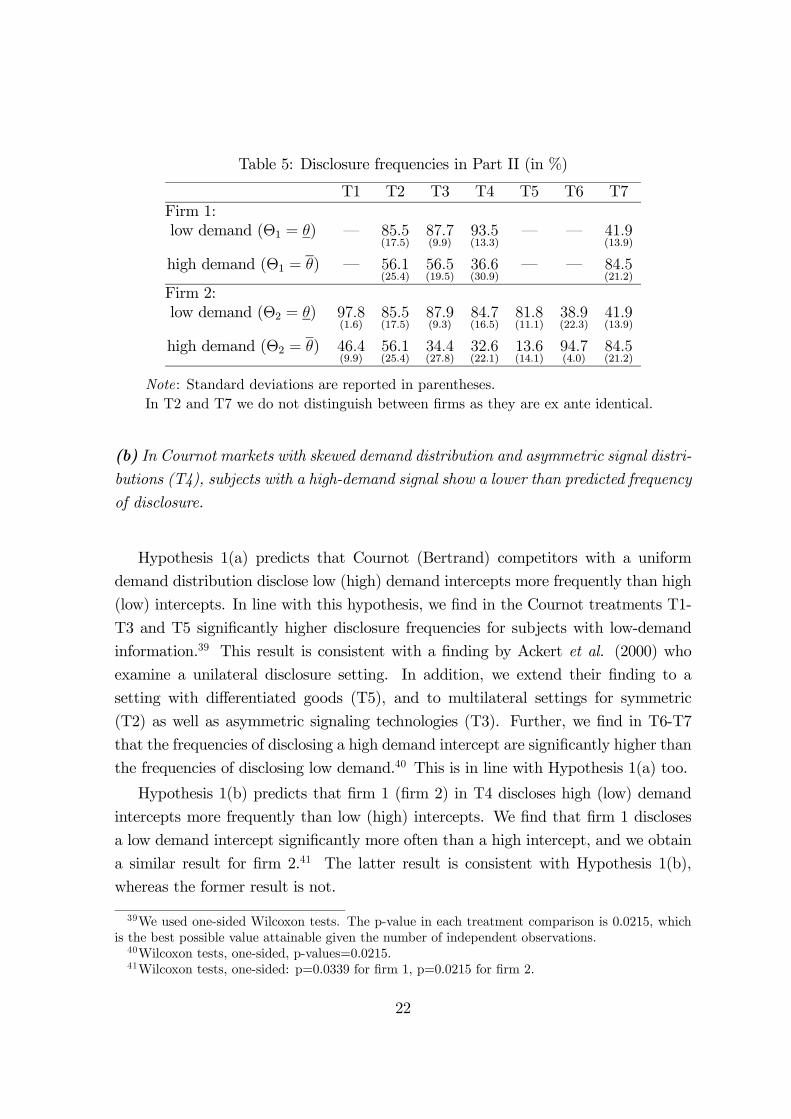
Table 5: Disclosure frequencies in Part II (in %)

T1 T2 T3 T4 T5 T6 T7

Firm 1:

low demand (Θ1 = ) – 855(175)

877(99)

935(133)

– – 419(139)

high demand (Θ1 = ) – 561(254)

565(195)

366(309)

– – 845(212)

Firm 2:

low demand (Θ2 = ) 978(16)

855(175)

879(93)

847(165)

818(111)

389(223)

419(139)

high demand (Θ2 = ) 464(99)

561(254)

344(278)

326(221)

136(141)

947(40)

845(212)

Note: Standard deviations are reported in parentheses.

In T2 and T7 we do not distinguish between firms as they are ex ante identical.

(b) In Cournot markets with skewed demand distribution and asymmetric signal distri-butions (T4), subjects with a high-demand signal show a lower than predicted frequency

of disclosure.

Hypothesis 1(a) predicts that Cournot (Bertrand) competitors with a uniform

demand distribution disclose low (high) demand intercepts more frequently than high

(low) intercepts. In line with this hypothesis, we find in the Cournot treatments T1-

T3 and T5 significantly higher disclosure frequencies for subjects with low-demand

information.39 This result is consistent with a finding by Ackert et al. (2000) who

examine a unilateral disclosure setting. In addition, we extend their finding to a

setting with differentiated goods (T5), and to multilateral settings for symmetric

(T2) as well as asymmetric signaling technologies (T3). Further, we find in T6-T7

that the frequencies of disclosing a high demand intercept are significantly higher than

the frequencies of disclosing low demand.40 This is in line with Hypothesis 1(a) too.

Hypothesis 1(b) predicts that firm 1 (firm 2) in T4 discloses high (low) demand

intercepts more frequently than low (high) intercepts. We find that firm 1 discloses

a low demand intercept significantly more often than a high intercept, and we obtain

a similar result for firm 2.41 The latter result is consistent with Hypothesis 1(b),

whereas the former result is not.

39We used one-sided Wilcoxon tests. The p-value in each treatment comparison is 0.0215, which

is the best possible value attainable given the number of independent observations.40Wilcoxon tests, one-sided, p-values=0.0215.41Wilcoxon tests, one-sided: p=0.0339 for firm 1, p=0.0215 for firm 2.

22

Result 1(a) suggests that the subjects understand that their disclosure reveals in-

formation to their competitor about the size of the market. That is, the subjects

seem to understand the strategic value of managing the competitor’s belief about the

market. In addition, it gives experimental support for the theoretical finding that the

disclosure behavior of Cournot competitors differs from that of Bertrand competitors

(e.g., Darrough, 1993). However, there is no evidence that subjects understand that

their disclosure reveals information about their own conduct, as Result 1(b) implies.

These observations are consistent with the observations by Ackert et al. (2000). Also

they find that subjects adjust their disclosure choices if they inform the competitor

about the market (industry-wide information), whereas they do not adjust if disclo-

sure informs the competitor about the discloser’s conduct (firm-specific information).

Ackert et al. make this observation in a model with unilateral disclosure of indepen-

dently distributed costs, whereas we make our observation in a model with bilateral

disclosure of a common demand intercept.

Disclosure choices in Part III For a deeper inquiry of the disclosure behavior,

we asked the participants in Part III of each treatment for a complete disclosure

strategy. Table 6 gives the frequencies of the individual disclosure-strategy choices

for each treatment and role in Part III. Out of the 90 participants who had to make

a disclosure decision in the Cournot treatments T1-T3 and T5, 42 subjects choose to

disclose only if demand is low, which is the equilibrium disclosure strategy. Another

39 (7) subjects choose to disclose all (no) demand intercepts. The high frequency of

full-disclosure choices is in line with Cai and Wang (2006), who find that senders in a

cheap-talk game tend to overcommunicate.42 Just 2 subjects choose to disclose only

a high demand intercept. In short, 90% of the subjects in Part III of T1-T3 and T5

disclose a low demand intercept, whereas less than 46% disclose a high intercept. This

is in line with Hypothesis 1(a). Also the frequencies from the Bertrand treatments

T6-T7 are in line with the aggregate disclosure predictions from Hypothesis 1(a), and

they are consistent with our findings from Part II.43

For T4, Hypothesis 1(b) predicts that firm 1 discloses a high demand intercept

42Subjects may disclose all information if they lack sophistication to recognize the strategic role of

information (Cai and Wang, 2006). Alternatively, subjects may have an aversion to deception (e.g.,

Gneezy, 2005), and they may interpret concealment as lying about the fact that they are informed.

Finally, risk-averse subjects may disclose all information to eliminate strategic uncertainty.43Out of the 45 subjects in T6-T7 who choose a disclosure strategy, 28 subjects choose to disclose

only a high demand intercept, whereas no subject chooses to do the reverse. Further, 14 (3) subjects

choose to disclose all (no) demand information. In other words, more than 93% of the subject choose

to disclose a high demand intercept, whereas about 31% disclose a low intercept.

23

Table 6: Frequencies of disclosure choices in Part III (in %)

T1 T2 T3 T4 T5 T6 T7

Firm 1’s strategy [1() 1()]

“disclose nothing” [0 0] – 6.7 6.7 6.7 – – 10

“disclose only low” [1 0] – 40 26.7 66.7 – – 0

“disclose only high” [0 1] – 3.3 0 13.3 – – 63.3

“disclose all” [1 1] – 50 66.7 13.3 – – 26.7

Firm 1’s disclosure frequency

low demand (Θ1 = ) – 90 93.3 80 – – 26.7

high demand (Θ1 = ) – 53.3 66.7 26.7 – – 90

Firm 2’s strategy [2() 2()]

“disclose nothing” [0 0] 0 6.7 26.7 6.7 0 0 10

“disclose only low” [1 0] 46.7 40 60 66.7 66.7 0 0

“disclose only high” [0 1] 0 3.3 0 0 6.7 60 63.3

“disclose all” [1 1] 53.3 50 13.3 26.7 26.7 40 26.7

Firm 2’s disclosure frequency

low demand (Θ2 = ) 100 90 73.3 93.3 93.3 60 26.7

high demand (Θ2 = ) 53.3 53.3 13.3 26.7 33.3 100 90

Note: In T2 and T7 we do not distinguish between firms as they are ex ante identical.

more frequently than a low intercept, whereas firm 2 does the reverse. However, Table

6 indicates that firm 1 chooses to disclose low-demand information more often (i.e., in

80% of the cases) than high-demand information (by less than 27% of the subjects).44

Hence, the behavior of subjects in the role of firm 1 is inconsistent with the predicted

behavior, whereas the behavior of firm 2 in T4 is consistent with our prediction.45

4.2.3 Observations on Product-Market Choices

Tables 7 and 8 summarize the average product-market choices in Part II of firm 1

and firm 2, respectively. These choices are output levels in T1-T5, whereas they are

44From the 15 subjects with the role of firm 1, there are 2 subjects who choose to disclose only

high demand, whereas 10 subjects choose to do the reverse. There are 2 (1) subjects with the role

of firm 1 who commit to disclosing all (no) information.45Out of the 15 subjects with the role of firm 2, 10 subjects commit to disclosing only low demand

intercepts, whereas no-one commits to the opposite strategy. Further, 4 (1) subjects in the role of

firm 2 commit to disclose all (no) information. Hence, low demand intercepts are disclosed by 93%

of the subjects, whereas high intercepts are disclosed by less than 27% of the subjects.

24

prices in T6-T7. We distinguish settings in which no messages were sent from settings

of complete information. In the former situation, firms did neither send nor receive

any informative message but they received a particular signal by nature. We list the

average product-market choices for this setting in the first three columns of Tables 7

and 8.46 We list the average product-market choices under complete information in

the last two columns of Tables 7 and 8. Here, we pool data from instances in which

firm 1, firm 2, and both firms sent an informative message.

Table 7: Average product-market choices of Firm 1 in Part II

Incomplete Information Complete Information

Θ1 = Θ1 = ∅ Θ1 = = =

T1 – 1053(77)

– 852(78)

1085(108)

T2 too few obs. 950(114)

1080(61)

816(26)

1018(41)

T3 too few obs. 999(39)

1127(16)

809(34)

1043(53)

T4 too few obs. 909(110)

1073(103)

796(111)

999(117)

T5 – 1205(125)

– 959(66)

1251(76)

T6 – 792(39)

– 743(72)

1057(69)

T7 758(74)

825(92)

too few obs. 783(67)

1065(60)

Note: Standard deviations are reported in parentheses.

In T2 and T7 we do not distinguish between firms as they are ex ante identical.

The choices in T1-T5 (T6-T7) are output levels (prices).

Product-market choice of privately informed firms (H2) First, we analyze

the effect of incomplete information on the product-market choices of informed firms.

Our statistical analysis gives the following result.

Result 2 In Cournot markets, there is evidence that subjects who are privately in-

formed about high demand supply significantly more than subjects with complete in-

formation about high demand. In Bertrand markets, there is no significant difference

between prices of subjects with private and complete information about low demand.

46We do not have enough observations to give a meaningful average for subjects who have learned

that demand is low (high) and have incomplete information in T1-T5 (respectively, T6-T7).

25

Table 8: Average product-market choices of Firm 2 in Part II

Incomplete Information Complete Information

Θ2 = Θ2 = ∅ Θ2 = = =

T1 too few obs. 938(63)

1111(94)

835(45)

1012(112)

T2 too few obs. 950(114)

1080(61)

816(26)

1018(41)

T3 too few obs. 989(101)

1190(244)

823(46)

1071(117)

T4 too few obs. 928(60)

1094(77)

779(45)

1101(90)

T5 too few obs. 1046(43)

1296(113)

916(72)

1224(179)

T6 763(58)

875(68)

too few obs. 808(30)

1043(51)

T7 758(74)

825(92)

too few obs. 783(67)

1065(60)

Note: Standard deviations are reported in parentheses.

In T2 and T7 we do not distinguish between firms as they are ex ante identical.

The choices in T1-T5 (T6-T7) are output levels (prices).

The pairwise comparison between the third and fifth columns of Tables 7 and 8 for

T1-T3 and T5 suggests that a firm with a high-demand signal chooses a higher output

level under incomplete information than under complete information. This is consis-

tent with Hypothesis 2(a), and it suggests that a firm with high-demand information

may have indeed an incentive to conceal its information. We also test whether there is

a statistically significant difference between the product-market choices under incom-

plete and complete information. The tests confirm that outputs differ significantly for

both firms in T2 and T3.47

Hypothesis 2(b) predicts that a firm 1 with a low-demand signal in T4 chooses

a lower output level under complete information than under incomplete information.

This requires that firm 1 did not receive an informative message by its competitor and

successfully learned the market demand by nature. This situation is unlikely to occur

for three reasons. First, firm 2 learns the market demand with 90% probability, and

it discloses low signals in equilibrium. Second, firm 1 has only a 30% probability of

learning the market demand by nature. Finally, firm 1 often disclosed a low demand

in the experiment. As a result, we lack sufficient observations to test Hypothesis 2(b).

47All p-values for the one-sided Wilcoxon tests in T2 and T3 are smaller than or equal to 0.0398.

By contrast, the differences between ∗2(; ·) and 2() are not significant in T1 (p-value=0.1124),and T4 (p-value=0.3429). Table 9 in the Appendix gives all the p-values for these tests.

26

With Bertrand competition, Hypothesis 2(c) predicts that the price of a firm with

low-demand information is higher with incomplete information than with complete

information. The pairwise comparison between the first and fourth columns of Tables

7 and 8 for T6 and T7 suggests that the reverse holds. However, from a statistical

point of view, the prices do not differ significantly in either treatment.

Product-market choices of uninformed firms (H3) Next, we characterize the

output choices of uninformed firms. Hypothesis 3 predicts that the product-market

choice of an uninformed firm should lie between the choices under complete informa-

tion for T1-T3, T4 for firm 1, and T5-T7. That is, the entries in the second column

are predicted to be greater (smaller) than the corresponding entries in the fourth

(fifth) column of Tables 7 and 8. The qualitative pairwise comparisons of our data

are consistent with the predicted rankings in all instances. Our statistical tests on

the variable differences are largely in line with these observations, as we state below.

Result 3 There is evidence that the product-market choices of uninformed subject

are significantly higher (lower) than the choices of subject with complete information

about a low (high) demand under the conditions of Hypothesis 3.

We test whether and how the average product-market choice of an uninformed firm

differs from the average product-market choices of a firm with complete information.

The first and third (second and last) columns of Table 10 in the Appendix give the

p-values for these comparisons when demand is low (high). The statistical inference

yields significant results in most cases.48 Hence, our observations are in line with

Hypothesis 3 in almost all cases.

The effect of a firm’s own signal precision (H4) For the uniform demand dis-

tribution, Hypothesis 4 predicts that a firm’s product-market choice under incomplete

information tends to be decreasing in the firm’s likelihood of receiving information.

This is the case for an uninformed firm. In addition, it happens if a Cournot com-

petitor is privately informed about high demand and it receives this information with

a high likelihood, or a Bertrand competitor has private low-demand information.

48Except for two tests, our results are significant with p-values smaller than or equal to 0.0398 for

the one-sided Wilcoxon tests. The two exceptions emerge for the comparisons of output choices by

uninformed subjects with output choices under complete information about high demand. There,

our results are not significant in T2 (p-value=0.1124), and weakly significant for firm 1 in T3 (p-

value=0.0690). Table 10 in the Appendix gives all p-values for the one-sided Wilcoxon tests.

27

In T1-T3, we vary firm 1’s likelihood of receiving information (1) for a Cournot

competitor with a uniform demand distribution (see Table 1). There is a ceteris

paribus increase in firm 1’s likelihood by moving from T1 (1 = 0%) via T3 (1 = 30%)

to T2 (1 = 90%). As Hypothesis 4(a) predicts, the qualitative comparison of the

incomplete-information entries in rows T1, T3 and T2 of Table 7 suggests a decreasing

pattern. Likewise, 1 increases from 0 to 09 for a Bertrand competitor by switching

from T6 to T7. In contrast to the prediction of Hypothesis 4(b), the comparison of

price choices under incomplete information (i.e., the second entry) in T6 and T7 of

Table 7 suggests that firm 1’s price increases in 1. In addition to these qualitative

comparisons, we perform statistical tests. This gives the following results.

Result 4 In Cournot markets, there is weak evidence that the output of subject

is decreasing in the subject’s likelihood of receiving information, , if the subject

remained uninformed or concealed high demand. In Bertrand markets, there is no

significant difference between the prices set by subjects with different likelihoods of

receiving information.

First, the decrease of outputs chosen by an uninformed firm 1 is weakly significant

if the firm’s signal precision 1 increases from 0% to 90%.49 For smaller increases of

1, the decrease in output is statistically insignificant (see the first column of Table

11 in the Appendix for details). Second, also the decrease in output of privately

informed firm 1 with Θ1 = is weakly significant.50 Hence, the qualitative and

statistical comparisons are in line with the prediction from Hypothesis 4(a), although

the statistical result is weak.

Hypothesis 4(b) predicts that firm 1’s prices are decreasing in signal precision 1,

whereas the qualitative comparison of average price choices in T6 and T7 of Table

7 suggests the reverse. Although the MWW test indicate that these prices do not

significantly differ from one another, our finding is not in line with Hypothesis 4(b).51

5 Conclusion

This paper analyzes a theoretical model and an experiment to examine voluntary

disclosure of demand information and product-market strategies in duopoly.

49One-sided MWW test: p-value=0.0586.50One-sided MWW test: p-value=0.0872.51Two-sided MWW test: p-value=0.9168.

28

The model extends some existing theoretical models dealing with simultaneous

disclosure choices by duopolists by allowing firms to be asymmetric. We identify con-

ditions for a Cournot duopoly under which firms choose the usual selective disclosure

strategy, with disclosure of low demand and concealment of high demand. In addition,

we give conditions under which one firm in an asymmetric Cournot duopoly chooses

the reverse information-disclosure strategy in equilibrium. Further, we show that

Bertrand competitors disclose high-demand information and conceal low demand.

Our experiment considers information-disclosure and product-market choices, and

the interaction between these choices too. The experiment’s treatments consider uni-

lateral disclosure, and bilateral disclosure in symmetric settings as well as asymmetric

settings. Thereby, we replicate a result of Ackert et al. (2000), and we extend it by

considering bilateral disclosure in addition to unilateral disclosure, Bertrand compe-

tition besides Cournot competition, and product differentiation.

A key finding is that subjects in the laboratory experiment often selectively disclose

their information. This finding is robust to changes in the information structure,

mode of competition, and the degree of product differentiation. On the one hand,

the subjects’ disclosure behavior suggests that the subjects understand that disclosed

information informs their competitor about the competitor’s demand. Their behavior

suggests that they often try to manage expectations of their competitor about the size

of the market demand to obtain a favorable product market choice of their competitor.

On the other hand, the subjects in our experiment did not seem to grasp that their

disclosed information also gives a signal to their competitor about their product-

market conduct. In a different context, also Ackert et al. (2000) observe that subjects

in the laboratory tend to ignore the signaling role of their information. They make this

observation in a model with unilateral disclosure of independently distributed costs,

whereas our model considers bilateral disclosure of a common demand intercept.

Moreover, our theoretical analysis tends to provide good qualitative predictions

for behavior in a duopolistic product market with demand uncertainty. The product-

market choices for subjects in our experiment tend to adjust to the subject’s infor-

mation, and they weakly adjust to the precision of information.

Our findings can be used as a starting point for understanding the impact of disclo-

sure regulation on information transmission and product market competition. These

theoretical and experimental findings can help to evaluate the effects of economic

policy towards information exchange, such as competition policy or accounting rules.

29

A Appendix

This Appendix contains the proofs of Propositions 1-4, the tables with test statistics

of Hypotheses 2-4, and the instructions of the experiment.

A.1 Proofs of Propositions

Proof of Proposition 1

The equilibrium output levels follow from solving the system of equations (9) and (8)

for Θ ∈ { } and = 1 2 with 6= . Details of the proof are relegated to the

Supplementary Appendix.

Proof of Proposition 2

First, consider equilibrium strategies such that ( ) = 0. That is, suppose that

firm chooses£() ()

¤in equilibrium, and the firm has beliefs consistent with the

competitor’s strategy£() ()

¤, such that firm is indifferent between disclosure

and concealment of its information. Using (12), the equation ( ) = 0 gives:

1− () =(1− )() [1− ()] [1− ()]

£1− ()

¤

(A.1)

where

≡ 2(1− ){1− ()} [1− ()]− (1− )()£1− ()

¤[1− ()]

(A.2)

Inequality 1− () 0 implies that 0. Substitution of (A.1) in (12) gives:

( ) = () [1− ()] [1− ()] (1− )1

[(1− ) + ]

where

≡ + ()(1− )£1− ()

¤ £1− ()

¤(A.3)

and

≡ 2£1− ()

¤ ¡ + ()(1− ) [1− ()]

£1− ()

¤¢−2(1− ) [1− ()]

£1− ()

¤ {1− ()} (A.4)

It is straightforward to show that (1−)+ 0 for any and (see the Supple-

mentary Appendix for details). This implies that if ( ) = 0, then ( ) 0.

30

Second, consider equilibrium strategies such that ( ) 0. That is,£() ()

¤=

(0 1) in equilibrium and beliefs are consistent with this strategy and some strategy£() ()

¤. Using (12), the inequality (0 1 () ()) 0 gives with:

≡ () [1− ()]

£1− ()

¤+ ()

£1− ()

¤[1− ()]

()£1− ()

¤[1− ()]

(A.5)

Suppose that (() () 0 1) ≤ 0. By (12), this inequality gives ≥ with:

≡2 [1− ()]

() [2 (1− ()) + (1− )](A.6)

Under these conditions, the existence of an equilibrium requires that ≤ . By

(A.5), (A.6) and () = 1− (), this inequality is equivalent to A(()) ≥ 0, where:A(()) ≡ ¡£

1− ()¤[1− ()]

£1− ()

¤+ ()

£1− ()

¤[1− ()]

¢∗ [2 (1− ()) + (1− )]− 2 [1− ()]

2 £1− ()¤

Notice that A is linear in (). Evaluating A for ()→ 1 gives the following:

A(1) =£1− ()

¤ [1− ()] [2 (1− ()) + (1− )]

−2 [1− ()]2 £1− ()

¤=

£1− ()

¤(1− ) ( [1− ()]− 2 [1− ()])

= − £1− ()¤(1− ) (2(1− ) + (2− ) [1− ()])

0

Clearly, in (A.6) is decreasing in (), and the extreme value for () at which

= 1 equals ≡ 2[1−()]2[1−()]+(1−) . Taking ()→ gives the following:

A() = (1− ) [1− ()] £1− ()

¤+2 [1− ()]

£1− ()

¤ [1− ()]− 2 [1− ()]

2 £1− ()¤

= − [1− ()]¡2£1− ()

¤(1− )− (1− )

£1− ()

¤¢= − [1− ()] (1− )

¡2(1− ) + (2− )

£1− ()

¤¢ 0

Then, linearity of A in () implies that A 0 for all ≤ () 1. However, this

implies that , and therefore (() () 0 1) ≤ 0 is not possible. In otherwords, if (0 1 () ()) 0 in equilibrium, then (() () 0 1) 0.

In conclusion, in any equilibrium there is always a firm with ( ) 0. Then

it follows from Proposition 1 that ∗ (; ) () and ∗ (; ) (), which

implies that the optimal disclosure strategy for firm is£() ()

¤= (1 0).

31

Proof of Proposition 3

Due to Proposition 2, we assume that firm chooses disclosure strategy£∗()

∗()

¤=

(1 0), and firms have beliefs consistent with£∗()

∗()

¤without loss of generality.

Hence, we adopt this assumption throughout the proof. Then, for some strategy£() ()

¤, the function from (12) reduces as follows:

([() ()] [1 0]) = (1− )(1− )¡() [1− ()] (1− ) + ()

£1− ()

¤¢+2(1− ) [1− ()]

£1− ()

¤ £() (1− ) + ()

¤−(1− ) (1− )

¡() [1− ()] + ()

£1− ()

¤¢= (1− ) [1− ()]

· ¡2 £1− ()¤[1− ()]− (1− )()

¢ (A.7)

(a) Also assume that firms have beliefs consistent with£() ()

¤= [1 0]. Then

Proposition 1 implies that ∗ (; [1 0] [1 0]) ≤ () and ∗ (; [1 0] [1 0]) ≥ () if

and only if ([1 0] [1 0]) ≥ 0. It follows from (A.7) that (1 0 1 0) ≥ 0 if and only if2 [1− ()] ≥ () (1− ) , which can be rewritten as 2 ≥ () [2 + (1− )].

(b) Now suppose that firms have beliefs consistent with£() ()

¤= [0 1]. Then it

follows from Proposition 1 that it is optimal for firm to conceal Θ = and disclose

Θ = if and only if ([0 1] [1 0]) ≤ 0. By (A.7), the inequality ([0 1] [1 0]) ≤ 0holds if and only if (2 + )() ≥ 2.(c) Here we assume that firms have beliefs consistent with some

£∗ ()

∗ ()

¤. Then

firm is indifferent between disclosure and concealment if and only if ([∗ ()

∗ ()] [1 0]) =

0. Hence, (A.7) implies that the equation ([∗ ()

∗ ()] [1 0]) = 0 is equivalent to

0 ≤ ∗ () ≤ 1 and:∗ () =

1

µ1− (1− )()

2 [1− ()]

¶Feasibility requires that ∗ () ≥ 0, which the reduces to () [2 + (1− )] ≤ 2,

and ∗ () ≤ 1, which reduces to ()(2 + ) ≥ 2.(d) Finally, firm can neither strictly prefer to disclose all demand information, nor

can the firm strictly prefer to conceal all information. This observation is due to the

fact that (12) can only have a single sign. This completes the proof.

Proof of Proposition 4

The proof is analogous to the proofs with Cournot competition (Propositions 1 and

3). The Supplementary Appendix contains details of the proof.

32

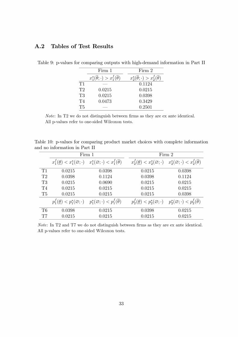
A.2 Tables of Test Results

Table 9: p-values for comparing outputs with high-demand information in Part II

Firm 1 Firm 2

∗1(; ·) 1() ∗2(; ·) 2()T1 – 01124T2 00215 00215T3 00215 00398T4 00473 03429T5 – 02501

Note: In T2 we do not distinguish between firms as they are ex ante identical.

All p-values refer to one-sided Wilcoxon tests.

Table 10: p-values for comparing product market choices with complete information

and no information in Part II

Firm 1 Firm 2

1() ∗1(∅; ·) ∗1(∅; ·) 1() 2() ∗2(∅; ·) ∗2(∅; ·) 2()

T1 00215 00398 00215 00398T2 00398 01124 00398 01124T3 00215 00690 00215 00215T4 00215 00215 00215 00215T5 00215 00215 00215 00398

1() ∗1(∅; ·) ∗1(∅; ·) 1() 2() ∗2(∅; ·) ∗2(∅; ·) 2()

T6 00398 00215 00398 00215T7 00215 00215 00215 00215

Note: In T2 and T7 we do not distinguish between firms as they are ex ante identical.

All p-values refer to one-sided Wilcoxon tests.

33

Table 11: p-values for comparing firm 1’s outputs across T1-T3 in Part II

Incomplete Information

Θ1 = ∅ Θ1 = 1(·;T1) 1(·;T3) 01736 –

1(·;T3) 1(·;T2) 03007 008721(·;T1) 1(·;T2) 00586 –

Note: The p-values correspond to one-sided MWW tests.

A.3 Instructions

These instructions are translated from the German instructions for the treatments

with Cournot competition and homogeneous goods (T1-T4). Naturally, neither the

treatment names, nor the parameter values of the other treatments were part of the

original instructions. Parts I and II of the instructions were followed by quiz questions

to ensure that all subjects understood the instructions. These questions are relegated

to the Supplementary Appendix. The instructions for the remaining treatments (i.e.,

T5 with differentiated goods, and T6-T7 with Bertrand competition) slightly modify

these instructions, and they are relegated to the Supplementary Appendix too.52

A.3.1 Instructions General Information

Welcome to the experiment!

In this experiment, you can earn money. How much you will earn depends on your

decisions as well as on the decisions taken by other participants. Regardless of your

decisions during the experiment, you will receive an additional 2.50 Euro for your

presence.

The experiment consists of three parts. Before each part, you receive precise instruc-

tions. All decisions taken during the course of this experiment are payout relevant.

During the experiment, the currency ECU (Experimental Currency Units) is used.

At the end of the experiment, all amounts in ECU are converted into Euro and paid

to you in cash. The exchange rate is 1 Euro for {T1-T3: 28,000; T4: 23,000} ECU.

Amounts are rounded up to full 10 Cent in your favor.

All decisions which you make during the experiment are anonymous. Your payout at

the end of the experiment is confidential.

52The complete instructions of all treatments are available in German upon request

(pollak@wiso.uni-koeln.de).

34

Please do not communicate any more with the other participants from now on. In

case you have any questions, now or during the experiment, please raise your hand.

Then we will come to you and answer your question. Please ensure additionally that

your mobile phone is switched off. Material (books, lecture notes, etc.), which does

not concern the experiment, may not be used during the experiment. Non-compliance

with these rules can lead to exclusion from the experiment and all payouts.

The following instructions refer to the first part. After the end of the first part, you

receive further instructions.

A.3.2 Instructions Part I

Part I of the experiment consists of 20 rounds which proceed in identical manner:

In this part of the experiment, you interact as producer with another participant, your

competitor. Your competitor is randomly matched to you. Each round this random

matching is done anew. We ensure that you never have the same competitor in two

consecutive rounds.

You and your competitor produce identical goods for a common market. Each pro-

duced good is sold at market price.

The market price is computed from the market demand minus the quantity produced

by you and your competitor:

⇒Market Price = Market Demand — Your Quantity — Competitor’s QuantityHowever, the market price cannot be smaller than zero. If the produced quantity

exceeds the market demand, then the market price equals zero.

Each round the market demand is determined by chance. The market demand is low

with a probability of {T1-T3: 50%; T4: 90%} and amounts to 240. With a probability

of {T1-T3: 50%; T4: 10%} it is high and amounts to 300. The positive market price

is thus given by:

⇒ if market demand is high:

Market Price = 300 — Your Quantity — Competitor’s Quantity

⇒ if market demand is low:

Market Price = 240 — Your Quantity — Competitor’s Quantity

At the beginning of each round, you learn after a few seconds whether the market

demand is high or low. The competitor also learns whether the market demand is

high or low. Afterwards, you choose your quantity (if applicable, including decimal

35

places). The competitor chooses his quantity simultaneously. While making these

choices, neither you nor your competitor can see what quantity the other chooses.

The market price is determined after you and your competitor have chosen the pro-

duction quantities. Your profit is determined by your quantity, which is sold at market

price. Neither you nor your competitor have to bear production costs.

⇒ Profit = Market Price × Your QuantityAt the end of each round, you will be informed about your profit for that round, the

market price, and the chosen quantities.

At the end of the experiment, the profits over all rounds will be converted into EURO

and paid out to you.

A.3.3 Instructions Part II

This part of the experiment is an extension of the first part. From now on, you do

not always know the market demand. If you do know the market demand, you can

choose to announce it to the competitor. The same applies for your competitor. The

matching of competitors is done as in Part I.

Part II of the experiment consists of 50 rounds with identical proceeding:

As in the first part, the market demand is high with a probability of {T1-T3: 50%;

T4: 10%}, and low with a probability of {T1-T3: 50%; T4: 90%}. How high it

is in the current round is not automatically apparent to you. However, you and

your competitor run a market analysis each round. Whether it is successful is

randomly determined in each round anew:

Independent of the current market demand, and the market analysis of the competitor,

Your market analysis is successful or unsuccessful with a certain probability. In addi-

tion, you know the probability of success for the market analysis of your competitor,

but you do not know his result. The same holds for your competitor.

The probabilities of success, depending on your role, are:

Own market analysis Competitor’s market analysis

Successful Not successful Successful Not successful

Role A

{T1:0%}

{T2:90%}

{T3-T4:30%}

{T1:100%}

{T2:10%}

{T3-T4:70%}

90% 10%

Role B 90% 10%

{T1:0%}

{T2:90%}

{T3-T4:30%}

{T1:100%}

{T2:10%}

{T3-T4:70%}

36

In case of a successful market analysis, you learn how high the market demand is. If

you learned the level of the market demand, then it is correct in any case. In case the

market analysis is not successful, you will not learn the market demand.

After the market analysis is conducted, you can costlessly inform your

competitor about the market demand, provided that you learned it. Your

competitor can also choose to inform you about the result of his market analysis. All

information sent is always truthful. Sending false information is not possible.

• If you know whether the market demand is high, respectively low:

— You can “inform” your competitor. Your competitor then knows for

certain that the market demand is high, respectively low. In addition,

he knows that you learned the market demand.

— You can “not inform” your competitor. In this case, the competi-

tor only knows the market demand, if his own market analysis was

successful. The competitor does not know whether you learned the

market demand.

• If you do not know whether market demand is high, respectively low:

— You can solely “not inform” your competitor. In this case, the

competitor only knows the market demand, if his own market analysis

was successful. In addition, the competitor does not know whether

you learned the market demand.

Only after you and your competitor have decided to “inform” / “not (to) inform” the

other, information will be transferred.

In case you received information from the competitor and/or your own

market analysis was successful, then you know the market demand. If you

neither received information from the competitor nor was your own market analysis

successful, then you do not know the market demand.

The further course of this part is identical to the first part. You and your

competitor choose your quantities and are informed about the result for that round.

At the end of the experiment, the profits over all rounds are converted into EURO and

paid out to you.

37

A.3.4 Instructions Part III

This part is an extension of the experiment from Part II. Now, a department takes over

the task to “inform”/ “not (to) inform” the competitor. You instruct the department

in which cases the information should be transferred. The quantity decision is still

taken by yourself. The same applies for your competitor. The probabilities for the

market demand, your market analysis, and the market analysis of the competitor

remain as in Part II. The matching of competitors is still determined randomly.

Part III of the experiment consists of one round with the following proceeding:

At the beginning of the round, you do not know the result of your market analysis.

However, you give binding instructions to your internal department about

the instances in which it must inform the competitor about the market

demand, in case the market analysis is successful.

You have 4 options:

1. Never inform

The competitor only knows the market demand, if his market analysis was

successful. he does not know, whether you learned the market demand.

2. Only inform if market demand is low

Case 1: Market analysis is successful and market demand is low

Your competitor knows for certain, that the market demand is low. In

addition, the competitor knows that you learned how high the market de-

mand is.

Case 2: Market analysis is not successful and/or the market demand is high

The competitor only knows the market demand, if his own market analysis

was successful. He does not know whether you learned the market demand.

3. Only inform if market demand is high

Case 1: Market analysis is successful and market demand is high

The competitor knows for certain, that the market demand is high. In

addition, he knows that you learned how high the market demand is.

Case 2: Market analysis is not successful and/or the market demand is low

The competitor only knows the market demand, if his own market analy-

sis was successful. he does not know whether you learned how high the

market demand is.

4. Always inform

Case 1: Market analysis is successful

38

The competitor knows for certain, that the market demand is high/low.

In addition, he knows that you learned the market demand.

Case 2: Market analysis is not successful

The competitor only knows the market demand, if his own market analysis

was successful. he does not know whether you learned how high the market

demand is.

Hereafter, you are informed, as before, whether your market analysis was successful

and whether you received information from the competitor.

As in Part II, the decision about the production quantity follows. Subse-

quently, you are informed about the outcome of this round, as usual.

At the end of the experiment, the profits over all rounds are converted into EURO and

paid out to you.

References

Ackert, L.F., B.K. Church, and M.R. Sankar, 2000, “Voluntary Disclosure

under Imperfect Competition: Experimental Evidence,” International Journal of In-

dustrial Organization, 18, 81-105.

Benndorf, V., D. Kübler, and H-T. Normann, 2015, “Privacy Concerns, Volun-

tary Disclosure of Information, and Unraveling: An Experiment,” European Economic

Review, 75, 43-59.

Cai, H. and J.T-Y. Wang, 2006, “Overcommunication in Strategic Information

Transmission Games,” Games and Economic Behavior, 56, 7-36.

Darrough, M.N., 1993, “Disclosure Policy and Competition: Cournot vs. Bertrand,”

The Accounting Review, 68, 534-561.

Dye, R.A., 1985, “Disclosure of Nonproprietary Information,” Journal of Accounting

Research, 23, 123-145.

Dye, R.A., 2001, “An Evaluation of ‘Essays on Disclosure’ and the Disclosure Lit-

erature in Accounting,” Journal of Accounting and Economics, 32, 181-235.

Farrell, J., 1986, “Voluntary Disclosure: Robustness of the Unraveling Result, and

Comments on Its Importance,” in R.E. Grieson, ed., Antitrust and Regulation, Lex-

ington, MA: Lexington Books, 91-103.

39

Fischbacher, U., 2007, “z-Tree: Zurich Toolbox for Ready—Made Economic Exper-

iments,” Experimental Economics, 10, 171-180.

Gneezy, U., 2005, “Deception: The Role of Consequences,” American Economic

Review, 95, 384-394.

Greiner, B., 2004, “An Online Recruitment System for Economic Experiments,” in

Kremer K. and V. Macho, eds., Forschung und wissenschaftliches Rechnen. GWDG

Bericht 63, Gesellschaft für Wissenschaftliche Datenverarbeitung: Göttingen, Ger-

many, 79-93.

Gürerk, Ü., and R. Selten, 2012,“The Effect of Payoff Tables on Experimental

Oligopoly Behavior,” Experimental Economics, 15, 499-509.

Holt, C.A., 1985,“An Experimental Test of the Consistent-Conjecture Hypothesis,”

The American Economic Review, 75, 314-325.

Huck, S., H-T. Normann, and J. Oechssler, 1999,“Learning in Cournot Oligopoly

- An Experiment,” The Economic Journal, 109, C80-C95.

Huck, S., H-T. Normann, and J. Oechssler, 2004,“Two are few and four are

many: Number Effects in Experimental Oligopolies,” Journal of Economic Behavior

& Organization, 53, 435-466.

Hwang, H-S., 1993, “Optimal Information Acquisition for Heterogenous Duopoly

Firms,” Journal of Economic Theory, 59, 385-402.

Hwang, H-S., 1994, “Heterogeneity and the Incentive to Share Information in

Cournot Oligopoly Market,” International Economic Review, 35, 329-345.

Jansen, J., 2008, “Information Acquisition and Strategic Disclosure in Oligopoly,”

Journal of Economics & Management Strategy, 17, 113—148.

Jin, G.Z., M. Luca, and D. Martin, 2015, “Is No News (Perceived As) Bad News?

An Experimental Investigation of Information Disclosure,” NBER Working Paper, nr.

21099.

Jung, W-O., and Y.K. Kwon, 1988, “Disclosure When the Market is Unsure of

Information Endowment of Managers,” Journal of Accounting Research, 26, 146-153.

King, R.R., and D.E. Wallin, 1991a, “Market-Induced Information Disclosures:

An Experimental Markets Investigation,” Contemporary Accounting Research, 8, 170-

197.

40

King, R.R., and D.E. Wallin, 1991b, “Voluntary Disclosures When Seller’s Level

of Information is Unknown,” Journal of Accounting Research, 29, 96-108.

Kühn, K-U. and X. Vives, 1995, Information Exchanges among Firms and their

Impact on Competition, Luxembourg: Office for Official Publications of the European

Communities.

Kühn, K-U., 2001, “Fighting Collusion by Regulating Communication Between

Firms,” Economic Policy, 16, 167-204

Milgrom, P.R., 1981, “Good News and Bad News: Representation Theorems and

Applications,” Bell Journal of Economics, 12, 380-391.

Milgrom, P.R., 2008, “What the Seller Won’t Tell You: Persuasion and Disclosure

in Markets,” Journal of Economic Perspectives, 22, 115-132.

Milgrom, P.R. and J. Roberts, 1986, “Relying on the Information of Interested

Parties,” RAND Journal of Economics, 17, 18-32.

Okuno-Fujiwara, M., A. Postlewaite, and K. Suzumura, 1990, “Strategic In-

formation Revelation,” Review of Economic Studies, 57, 25-47.

Raith, M., 1996, “A General Model of Information Sharing in Oligopoly,” Journal

of Economic Theory, 71, 260-288.

Requate, T., and I. Waichman, 2011, “A Profit Table or a Profit Calculator?:

A Note on the Design of Cournot Oligopoly Experiments,” Experimental Economics,

14, 36-46.

Sankar, M.R., 1995, “Disclosure of Predecision Information in a Duopoly,” Contem-

porary Accounting Research, 11, 829-859.

Selten, R., 1967, “Die Strategiemethode zur Erforschung des eingeschränkt ratio-

nalen Verhaltens im Rahmen eines Oligopolexperimentes,” in Sauermann, H., ed.,

Beiträge zur Experimentellen Wirtschaftsforschung, J.C.B. Mohr (Paul Siebeck): Tübin-

gen, Germany, 136-168.

Siegel, S. and N.J. Castellan, 1988, Nonparametric Statistics for the Behavioral

Sciences - Second Edition, McGraw-Hill: New York, USA.

Verrecchia, R.E., 2001, “Essays on Disclosure,” Journal of Accounting and Eco-

nomics, 32, 97-180.

Vives, X., 1999, Oligopoly Pricing: Old Ideas and New Tools, Cambridge, MA: MIT

Press.

41