Strategic Decompositions of Normal Form Games: Zero-sum

Games and Potential Games

Sung-Ha Hwanga,∗, Luc Rey-Belletb

aKorea Advanced Institute of Science and Technology (KAIST), Seoul, KoreabDepartment of Mathematics and Statistics, University of Massachusetts Amherst, MA, U.S.A.

Abstract

We study new classes of games, called zero-sum equivalent games and zero-sumequivalent potential games, and prove decomposition theorems involving these classesof games. We say that two games are “strategically equivalent” if, for every player,the payoff differences between two strategies (holding other players’ strategies fixed)are identical. A zero-sum equivalent game is a game that is strategically equivalentto a zero-sum game; a zero-sum equivalent potential game is a zero-sum equivalentgame that is strategically equivalent to a common interest game. We also call a game“normalized” if the sum of one player’s payoffs, given the other players’ strategies,is always zero. We show that any normal form game can be uniquely decomposedinto either (i) a zero-sum equivalent game and a normalized common interest game,or (ii) a zero-sum equivalent potential game, a normalized zero-sum game, and anormalized common interest game, each with distinctive equilibrium properties. Forexample, we show that two-player zero-sum equivalent games with finite strategy setsgenerically have a unique Nash equilibrium and that two-player zero-sum equivalentpotential games with finite strategy sets generically have a strictly dominant Nashequilibrium.

Keywords: decomposition, zero-sum games, potential games.

JEL Classification Numbers: C72, C73

∗January 12, 2017. Corresponding author. The research of S.-H. H. was supported by theNational Research Foundation of Korea Grant funded by the Korean Government. The researchof L. R.-B. was supported by the US National Science Foundation (DMS-1109316). We would liketo thank Murali Agastya, Samuel Bowles, Yves Gueron, Nayoung Kim, Suresh Naidu, JonathanNewton, David Nielsen and Seung-Yun Oh for their helpful comments. Special thanks to WilliamSandholm who read the early version (http://arxiv.org/abs/1106.3552) of this paper carefullyand gave us many helpful suggestions.

Email addresses: sungha@kaist.ac.kr (Sung-Ha Hwang), luc@math.umass.edu (LucRey-Bellet)

1. Introduction

When two people start a joint venture, their interests are aligned. In the division

of a pie or unclaimed surpluses, however, someone’s gain always comes at the expense

of somebody else. So-called common interest games and zero-sum games serve as

polar models for studying these social interactions. Two games can be regarded

as “strategically equivalent” if, for every player, the payoff differences between two

strategies (holding other players’ strategies fixed) are identical. That is, in two

strategically equivalent games, strategic variables such as best responses of players

are identical.1 Potential games—a much studied class of games in the literature—

are precisely those games that are strategically equivalent to common interest games.

We also call a game “normalized” when the sum of one player’s payoffs, given the

other players’ strategies, is always zero.

We are interested in zero-sum games and their variants—(i) games that are strate-

gically equivalent to a zero-sum game, accordingly named zero-sum equivalent games,

(ii) zero-sum equivalent games which are, at the same time, equivalent to a com-

mon interest game, named zero-sum equivalent potential games and (iii) normalized

zero-sum games. Our interest in zero-sum equivalent games is motivated by their

analogous definitions to potential games. Potential games retain all the attractive

properties of common interest games (the existence of a pure strategy Nash equilib-

rium and a potential function) because they are strategically equivalent to common

interest games. Thus, zero-sum equivalent games are expected to retain similar desir-

able properties of zero-sum games as well. It is well-known that two-player zero-sum

games with a finite number of strategies have mini-max strategies and admit a value

of games which are useful tools for amenable analysis of equilibrium. Recently, there

have been generalizations of these properties and characterizations for a special class

of n-player zero-sum games (Bregman and Fokin (1998); Cai et al. (2015); see Section

3 for an extensive discussion of zero-sum equivalent games).

To study these classes of zero-sum related games, we develop decomposition meth-

ods of an arbitrary normal form game and obtain several constituent components

belonging to these classes and a special class of common interest games. Our de-

composition results provide (i) characterizations for zero-sum equivalent games as

1See Definition 2.2 and Monderer and Shapley (1996) and Weibull (1995); see also Morris andUi (2004) for best response equivalence.

1

4,4 -1,1 1,-11,-1 2,2 -2,0-1,1 0,-2 2,2

=2,2 -1,-1 -1,-1

-1,-1 2,2 -1,-1-1,-1 -1,-1 2,2︸ ︷︷ ︸

=C

+0,0 -1,1 1,-11,-1 0,0 -1,1-1,1 1,-1 0,0︸ ︷︷ ︸

=Z

+1,1 1,0 1,00,1 0,0 0,00,1 0,0 0,0︸ ︷︷ ︸

=B

+1,1 0,1 0,11,0 0,0 0,01,0 0,0 0,0︸ ︷︷ ︸

=E

Table 1: Illustration of our four-component decomposition. This example illustrates ourmain results. Here, C is a common interest game, Z is a zero-sum game (the Rock-Paper-Scissorsgame), B is a game in which the first strategy is the dominant strategy, and E is called a “non-strategic” game, in which, for every player, the payoff differences between two strategies (holdingother players’ strategies fixed) are identical (see Definition 2.1). Observe that C and Z are “nor-malized” in the sense that the column sums and row sums of the payoffs are zeros.

well as others (e.g., Propositions 3.2, 4.1, and 4.2) and (ii) decompositions of a given

game into components with distinctive equilibrium properties (Theorem 5.1, Figure

3). Intuitively, a decomposition of an arbitrary game gives an idea of how the original

game is “close” to component games with desirable properties.

Our main results (Theorem 2.1 (ii) and Proposition 4.1) show that every normal

form game can be decomposed into four components: (i) a “normalized” common

interest component (C in Table 1), (ii) a “normalized” zero-sum component (Z in

Table 1), (iii) a zero-sum equivalent potential component—component equivalent to

both a zero-sum and common interest game (B in Table 1), and (iv) a nonstrategic

component (E in Table 1). Most popular zero-sum games, such as Rock-Paper-

Scissors games and Matching Pennies games, belong to the class of normalized zero-

sum games (see also Cyclic games in Hofbauer and Schlag (2000)).

This study makes the following contributions. We develop a more general way

of decomposing normal form games than existing methods. Existing decomposition

methods of normal form games, such as in Hwang and Rey-Bellet (2011), Candogan

et al. (2011), and Sandholm (2010a), are limited to finite strategy set games, relying

on decomposition methods of tensors (or matrices) or graphs. Our new insights lie

in viewing the set of all games as a Hilbert space; we use a Hilbert space decom-

position technique and obtain decomposition results of normal form games at an

abstract level, which are applicable to games with continuous strategy sets as well

2

as those with finite strategy sets.2 In this way, our method shows a unified and

transparent mechanism of decompositions of games and can be easily modified to

decompose other classes of games such as Bayesian games. Further, many problems

in economics are modeled using continuous strategy games; thus our results, such

as the characterizations and the equilibrium properties of component games, can

be applied to a wide range of problems including, for example, Cournot games and

contest games.

Second, the concept of orthogonality in Hilbert space is useful in the sense that

we can naturally characterize a class of games by describing the games which are

orthogonal to it, that is their orthogonal complements. For example, the sufficiency

and necessity of the well-known Monderer and Shapley cycle condition for potential

games (Theorem 2.8 in Monderer and Shapley (1996)) can be proved by showing that

this condition requires that potential games are orthogonal to all the normalized

zero-sum games. We use the orthogonality which yields a unique decomposition

of a given game into a common interest game and a zero-sum game (Kalai and

Kalai, 2010) and into a normalized game and a non-strategic game (Hwang and Rey-

Bellet, 2011; Candogan et al., 2011). Based on this orthogonal decomposition, we are

able to provide characterizations of games, such as zero-sum equivalent games, zero-

sum potential games, normalized zero-sum games, and normalized common interest

games.

After our main decompositions in Section 2, we present detailed analyses of each

component game—zero-sum equivalent games, zero-sum equivalent potential games,

normalized zero-sum games, and normalized common interest games. In Section 3,

we show that zero-sum equivalent games have a Nash equilibrium and under some

(easily checkable) conditions they have a unique Nash equilibrium. We also show that

show that two-player zero-sum equivalent games with finite strategy sets generically

have a unique Nash equilibrium (Corollary 3.1). In Section 4, we study zero-sum

equivalent potential games. In particular, we show that two-player games in this

class generically possess a strictly dominant strategy (Corollary 4.3). This kind

of two-player game (game B in Table 1), which is strategically equivalent to both

2For example, the decomposition by Candogan et al. (2011) relies on the Helmholtz decompo-sition of flows on the graph for games with finite strategy sets and uses Moore inverses of matrixoperators. In fact, one of our previous decomposition results in Hwang and Rey-Bellet (2011) havesome overlaps with the main result in the cited paper.

3

Notations Names Definitions

C Common interest games Definition 2.1

Z Zero-sum games Definition 2.1

N Normalized games Definition 2.1

E non-strategic games (define Equivalence relation) Definition 2.1

Z + E Zero-sum Equivalent games Definition 2.4

C + E potential games (Common interest Equivalent games) Definition 2.3

B = (Both) zero-sum equivalent (and) potential games Definition 2.4

(Z + E) ∩ (C + E)

D games which have a Dominant strategy for two-player games Definition 4.1

N ∩ Z Normalized Zero-sum games

N ∩ C Normalized Common interest games

Table 2: Notations for the spaces of games.

a zero-sum game and a common interest game, only involves self-interactions, not

interactions between two players, since a player’s payoffs depend only on her own

actions.

Putting all this together, we provide a decomposition of a two player finite game

into component games, each possessing distinctive equilibrium characteristics (The-

orem 5.1). To help readers digest the main results, we keep some important proofs

in the text; however, to streamline the presentation, we relegate some lengthy and

tedious proofs to the appendix. Also, in Appendix A, we review the basic results

about the decomposition of a Hilbert space to provide theoretical background.

2. Decomposition Theorems

In this section, we present the basic setup, provide some preliminary results and

present our main decomposition theorems.

2.1. Basic setup

An n-player game (N,S, f) is specified by a set of players, N = {1, 2, · · · , n};a set of strategy profiles, S :=

∏ni=1 Si, where Si is a set of strategies for player

i; and a payoff function, f := (f (1), f (2), · · · , f (n)). For each i, f (i) : S → R is a

real-valued function, with f (i)(s) specifying the payoff for player i, given a strategy

profile, s = (s1, · · · , sn). We follow the convention of writing f (i)(si, s−i) = f (i)(s),

where s−i is the strategy profile of the players other than i. We associate a finite

4

measure space with each set of strategies, Si, as follows. If Si is a finite set, we let

mi be the counting measure with the natural σ-algebra of all subsets of Si. If Si is

a subset of Rdi for some di, we assume that Si is bounded and choose mi to be the

Lebesgue measure on Si with the Borel σ-algebra on Si. Thus, we have mi(Si) <∞.

We call a game with finite strategy sets simply a finite game to distinguish it from

continuous strategy games.

Given N and S, a game is uniquely specified by the vector-valued function f :=

(f (1), f (2), · · · , f (n)) which we assume to be measurable. We succinctly write an

n-fold integration as follows:∫f (i)dm =

∫· · ·∫f (i)(s1, · · · , sn)dm1(s1) · · · dmn(sn).

We define the norm of the payoff function f by

‖f‖ := (n∑i=1

∫ ∣∣f (i)∣∣2 dm)1/2

and consider the space of games to be

L := {f : S → Rn measurable and ‖f‖ <∞}. (1)

For finite games, the payoff functions can be represented as matrices (or tensors), and

L is the set of all matrices (or tensors) of suitable dimensions. Existing decomposition

methods, such as those of Hwang and Rey-Bellet (2011), Candogan et al. (2011) and

Sandholm (2010a), all focus on the case of finite strategy sets, while we consider

a general strategy space which can be either finite or continuous. We also follow

the usual convention of redefining L to be the set of all equivalent classes of almost

everywhere defined integrable functions on S. Thus, whenever we state a result for

a function, f , it holds for all its equivalent functions which agree with f almost

everywhere. Our choice of the norm turns L into a Hilbert space with a scalar

product

〈f, g〉 :=∑i

∫f (i)g(i)dm, (2)

which gives us 〈f, f〉 = ‖f‖2. We next introduce several classes of games of interest.

Definition 2.1. We define the following subspaces of L:

5

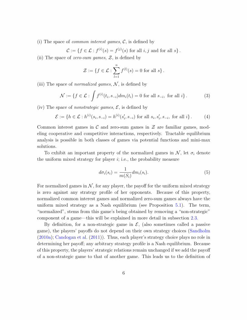
(i) The space of common interest games, C, is defined by

C := {f ∈ L : f (i)(s) = f (j)(s) for all i, j and for all s} .(ii) The space of zero-sum games, Z, is defined by

Z := {f ∈ L :n∑l=1

f (l)(s) = 0 for all s} .

(iii) The space of normalized games, N , is defined by

N := {f ∈ L :

∫f (i)(ti, s−i)dmi(ti) = 0 for all s−i, for all i} . (3)

(iv) The space of nonstrategic games, E , is defined by

E := {h ∈ L : h(i)(si, s−i) = h(i)(s′i, s−i) for all si, s′i, s−i, for all i} . (4)

Common interest games in C and zero-sum games in Z are familiar games, mod-

eling cooperative and competitive interactions, respectively. Tractable equilibrium

analysis is possible in both classes of games via potential functions and mini-max

solutions.

To exhibit an important property of the normalized games in N , let σi denote

the uniform mixed strategy for player i; i.e., the probability measure

dσi(si) =1

m(Si)dmi(si). (5)

For normalized games in N , for any player, the payoff for the uniform mixed strategy

is zero against any strategy profile of her opponents. Because of this property,

normalized common interest games and normalized zero-sum games always have the

uniform mixed strategy as a Nash equilibrium (see Proposition 5.1). The term,

“normalized”, stems from this game’s being obtained by removing a “non-strategic”

component of a game—this will be explained in more detail in subsection 2.3.

By definition, for a non-strategic game in E , (also sometimes called a passive

game), the players’ payoffs do not depend on their own strategy choices (Sandholm

(2010a); Candogan et al. (2011)). Thus, each player’s strategy choice plays no role in

determining her payoff; any arbitrary strategy profile is a Nash equilibrium. Because

of this property, the players’ strategic relations remain unchanged if we add the payoff

of a non-strategic game to that of another game. This leads us to the definition of

6

strategic equivalence (and thus notation, E).3

Definition 2.2. We say that game g is strategically equivalent to game f if

g = f + h for some h ∈ E

We write this relation as g ∼ f , and this is obviously an equivalence relation.

The class of potential games defined by Monderer and Shapley (1996) has received

much attention for its analytical convenience. Among the several equivalent defini-

tions for potential games we choose the one convenient for our purpose: potential

games are those that are strategically equivalent to common interest games.

Definition 2.3. The space of potential games (common interest equivalent games)is defined by

C + E . (6)

Recall that the notation f ∈ C+E means that f can be written as a linear combination

of a common interest game and a non-strategic game.

It is also well-known that two-player zero-sum games (as well as potential games)

have desirable properties—the value of a game, the mini-max theorem and so on. We

then expect that (i) two-player zero-sum equivalent games retain some of these prop-

erties and (ii) n-person zero-sum equivalent games may possess similar but possibly

weakened properties. As the example in Section 2.2 shows, n-player zero-sum equiv-

alent games have appealing properties, which can be useful for equilibrium analysis

(see Section 3). This leads us to consider the space of games that is strategically

equivalent to zero-sum games. Moreover, as both potential games and zero-sum

equivalent games have desirable properties, we will identify, as well, the class of

games which is simultaneously strategically equivalent to a common interest game

and a zero-sum game.

Definition 2.4. We have the following definitions:

3One can study different strategic equivalences. For example, Monderer and Shapley (1996)introduce the concept of w− potential games in which the payoff changes are proportional for eachplayer. Morris and Ui (2004) also study the best response equivalence of games in which playershave the same best-responses. We choose our definition of strategic equivalence since it is mostnatural with the linear structure of the space of all games.

7

(i) The space of zero-sum equivalent games is defined by

Z + E (7)

(ii) The space of games that is strategically equivalent to both a common interest

game and a zero-sum game, called zero-sum equivalent potential games, is denoted

by B.

2.2. Motivating examples

Example 1 (Strategic equivalence: Cournot oligopoly).

Consider a quasi-Cournot oligopoly game with a linear demand function for which

the payoff function for the i-th player, for i = 1, · · · , n, is given by

f (i)(s) = (α− βn∑j=1

sj)si − ci(si) ,

where α, β > 0, ci(si) ≥ 0 for all si ∈ [0, s] for all i and for some sufficiently large s.4

It is well-known that this game is a potential game (Monderer and Shapley 1996);

i.e., it is strategically equivalent to a common interest game but is also strategically

equivalent to a zero sum game (if n ≥ 3). To show this, when n = 3, we write the

payoff function asf (1)

f (2)

f (3)

=

(α− βs1)s1 − c1(s1)(α− βs2)s2 − c2(s2)(α− βs3)s3 − c3(s3)

︸ ︷︷ ︸

Self-Interaction

−

βs1s2βs1s20

︸ ︷︷ ︸Interactions

between players 1 and 2

−

βs1s30

βs1s3

︸ ︷︷ ︸Interactions

between players 1 and 3

−

0

βs2s3βs2s3

︸ ︷︷ ︸Interactions

between players 2 and 3

(8)

The self-interaction term is strategically equivalent to both a common interest

4Here, quasi-Cournot games allow the negativity of the price (Monderer and Shapley, 1996).Further, we can choose s to ensure that the unique Nash equilibrium lies in the interior [0, s]as follows. Suppose that ci(si) is linear; that is, ci(si) = cisi for all i. We assume that α >nmini ci − (n− 1) maxi ci, which ensures that the Nash equilibrium, s∗, is positive. If we choose ssuch that (n+ 1)βs > α− nmini ci + (n− 1) maxi ci, then s∗i ∈ (0, s) for all i.

8

game and a zero-sum game, as the following two payoffs show (α− βs1)s1 − c1(s1) +(α− βs2)s2 − c2(s2) +(α− βs3)s3 − c3(s3)(α− βs1)s1 − c1(s1) +(α− βs2)s2 − c2(s2) +(α− βs3)s3 − c3(s3)(α− βs1)s1 − c1(s1) +(α− βs2)s2 − c2(s2) +(α− βs3)s3 − c3(s3)

(9)

and (α− βs1)s1 − c1(s1)− [(α− βs2)s2 − c2(s2)](α− βs2)s2 − c2(s2)− [(α− βs3)s3 − c3(s3)](α− βs3)s3 − c3(s3)− [(α− βs1)s1 − c1(s1)]

. (10)

The payoffs in (9) and (10) are payoffs for a common interest game and a zero-sum

game, respectively. They are obtained from the self-interaction term by adding pay-

offs that do not depend on the player’s own strategy and thus they are strategically

equivalent (see Definition 2.2).

In a similar way, the payoff component describing the interactions between players

1 and 2 is strategically equivalent to the payoff for a common interest game and the

payoff for a zero-sum game. For example,βs1s2βs1s20

,

βs1s2βs1s2βs1s2

, and

βs1s2βs1s2−2βs1s2

(11)

are all strategically equivalent. A similar computation holds for the last two terms

in equation (8) involving the interactions between players 1 and 3 as well as between

players 2 and 3. As a consequence, the quasi-Cournot oligopoly game is strategically

equivalent to both a common interest game and a zero-sum game.

Example 2 (Zero-sum equivalent games: Contest games).

Our next example is a contest game (Konrad, 2009), which is a zero-sum equivalent

game. Consider an n-player game where the payoff function for the i-th player is

defined by

f (i)(s) = p(i)(si, s−i)v − ci(si) for i = 1, · · · , n, (12)

where∑

i p(i)(s) = 1 and p(i)(s) ≥ 0 for all s ≥ 0, ci(0) = 0, ci(·) is continuous,

increasing and convex and v > 0. First, f is a zero-sum equivalent game, since w,

9

defined by

w(i) = (p(i)(si, s−i)−1

n)v − 1

n− 1

∑j 6=i

(ci(si)− cj(sj))

for all i, is strategically equivalent to f and is itself a zero-sum game. In Section 3,

we will show that the following function, Φ(s), plays an important role in studying

the equilibrium property of zero-sum equivalent games:

Φ(s) := maxt∈S

n∑i=1

w(i)(ti, s−i) (13)

for s ∈ S. To illustrate our result, suppose that f (i)’s are given by a relatively simple

form:

f (i)(s) =si∑j sj

v − cisi. (14)

Then it is known that the game specified by (14) admits a unique Nash equilibrium

(Szidarovszky and Okuguchi, 1997). From the first order condition of equation (14),

we can find a best response s∗i (s−i)

ci(s∗i +

∑l 6=i

sl)2 = v

∑l 6=i

sl.

And via some computation, we find that

Φf (s) = (∑i

ci)(∑l

sl)− 2∑i

√civ

√∑l 6=i

sl + (n− 1)v (15)

which is strictly convex5. Later we show that if Φf for zero-sum equivalent game f is

strict convex, then f has a unique Nash equilibrium (Lemma 3.2 and Proposition 3.1).

This method of using the function Φ in equation (13), differently from the existing

5In fact, the best response function accounting for the boundary conditions, si ≥ 0, is given by

s∗i =

{0 if v

ci≤∑

l 6=i sl√vci

√∑l 6=i sl −

∑l 6=i s−l otherwise .

It can be shown that Φf defined for this function achieves the same minimum as the one in equation(15).

10

analysis relying on the special properties of the payoff functions (Szidarovszky and

Okuguchi, 1997; Cornes and Hartley, 2005), provide an alternative way of showing

the existence and uniqueness of equilibrium, hence can be extended to more general

settings.

Example 3 (Bayesian games). A Bayesian game with finite type spaces can be

viewed as a normal form game by defining a player with a specific type as a new

player (see the type-agent representation in Myerson (1997)). More specifically, con-

sider a two-player game, for which player 2 has two types, τ1 and τ2 :

(g(1), g(2)):=

player 2: τ1s′1 s′2

s1 a, a 0, 0

s2 0, 0 b, b

(h(1), h(2)) :=

player 2: τ2s′1 s′2

s1 a, b 0, 0

s2 0, 0 b, a

where (g(1), g(2)) and (h(1), h(2)) are the payoff functions, given types τ1 and τ2, re-

spectively. In this example, player 1 is not sure whether her partner has common

interests or conflicting interests. Suppose that τ1 and τ2 occur with probabilities p

and 1 − p, respectively. Then, we can introduce a new game in which players 1′,

2′, and 3′ are player 1 in the original game, player 2 with τ1, and player 2 with τ2,

respectively. The payoff function, f , for the new game is defined as follows :

f(s) =

f (1′)(s1, s2, s3)

f (2′)(s1, s2, s3)

f (3′)(s1, s2, s3)

=

g(1)(s1, s2)g(2)(s1, s2)

0

p+

h(1)(s1, s3)0

h(2)(s1, s3)

(1− p).

Here, the payoff function is based on the players’ ex-ante expected payoffs. That is,

the original player 1 ex-ante expects g(1)p+ h(1)(1− p), and the original player 2 ex-

ante expects the sum of the payoffs of players 2′ and 3′. Then, using manipulations

similar to those in the Cournot example, we see that f is strategically equivalent to

a zero-sum game. The reason is that each player’s payoff function is the sum of the

component games played among a subset of players (e.g., f (1′) = g(1)p+h(1)(1−p)). In

addition, we can show that if g = (g(1), g(2)) and h = (h(1), h(2)) are potential games,

which is straightforward to do, then f is itself a potential game (see Proposition

3.4). Therefore, the Bayesian game given in this example is a potential game and

is strategically equivalent to a zero-sum game. Later, we show that every Bayesian

11

game, embedded as a normal form game with more players, is strategically equivalent

to a zero-sum game in the resulting space of extended normal form games.

2.3. Preliminary results

For the purpose of exposition we present some preliminary results, some of which

are known and elementary, including some extensions of results from finite games to

continuous strategy games. The advantage of a Hilbert space structure is the natural

concept of orthogonality in terms of the inner product, 〈f, g〉, in (2): we say that

f and g are orthogonal if 〈f, g〉 = 0. In the context of game theory there are two

important orthogonality relations: (i) common interest games and zero-sum games

are orthogonal (Kalai and Kalai (2010)) and (ii) non-strategic games and normalized

games are orthogonal (Hwang and Rey-Bellet (2011); Candogan et al. (2011)). We

first state these two facts and explain their meanings and consequences.

Proposition 2.1. We have the decompositions of the space of all games:

L = C ⊕ Z (16)

L = N ⊕ E (17)

where the direct sum ⊕ means that every game has a unique decomposition into a

sum of two orthogonal components.

Proof. See Corollary in B.1 and see Appendix A for a formal definition of direct

sums.

The first orthogonality relation in (16) implies that common interest games and

zero-sum games are orthogonal to each other, that is

for all f ∈ C and g ∈ Z, 〈f, g〉 = 0, (18)

which is denoted by C ⊥ Z (this property is easy to check, using Fubini’s theorem).

Moreover, any given game f ∈ L can be uniquely written as f = c+z with c ∈ C and

z ∈ Z. Hence, f is a common interest game if and only if its zero-sum component

is z = 0, and f is a zero-sum game if and only if its common interest component is

c = 0. In this way, the concept of orthogonal projections allows us to identify and

12

separate the different components of a game, representing common and conflicting

interests, respectively.

To understand the second orthogonality relation, note the following simple, but

useful, characterization for a non-strategic game: a function does not depend on a

variable if and only if the value of the integral of the function with respect to that

variable gives the same value:

Lemma 2.1. A game f is a non-strategic game if and only if

f (i)(s) =1

mi(Si)

∫f (i)(ti, s−i)dmi(ti) for all i, for all s . (19)

Proof. Suppose that f satisfies (19). Then, clearly, f (i) does not depend on si for all

i. Now let f ∈ E . Then there exist ζ such that f (i)(s) = ζ(i)(s−i) for all s, which

does not depend on si, for all i. Thus, by integrating, we see that (19) holds.

Using the definition of normalized games in (3) and the characterization for non-

strategic games in (19), we can verify that

for all f ∈ E and g ∈ N , 〈f, g〉 = 0 (20)

which illustrates the decomposition in (17). Thus, any game payoff f can be uniquely

decomposed into n ∈ N and e ∈ E . The game n is called a normalized game since any

game f can be normalized such that it is equivalent to a game with a no non-strategic

component, i.e.,

f ∼ f − (1

m1(S1)

∫f (1)(s1, ·)dm1(s1), · · · ,

1

mn(Sn)

∫f (n)(sn, ·)dmn(sn)). (21)

To identify a potential game (C+ E , Definition 2.3), it is natural to examine how

any given game is “close” to a potential game by decomposing it into a potential

component and a component which fails to be a potential game, that is which is

orthogonal to a potential game. This leads to the decomposition in (22).

Proposition 2.2. We have the following decomposition:

L = (C + E)⊕ (N ∩ Z). (22)

Proof. For finite strategy games, this result easily follows from the decomposition

13

results of the Hilbert space, presented in Proposition A.2. For continuous strategy

games, the space (C + E) has to be closed, which we proved in Proposition B.1.

The decomposition in (22) shows that every game can be uniquely decomposed

into a potential component and a normalized zero-sum component. Examples of

normalized zero-sum games include the Rock-Paper-Scissors games and Matching

Pennies games, as explained in the introduction. The decomposition in (22) can

be regarded as a continuum version of the finite game decomposition in Candogan

et al. (2011). However, the difference between the two decompositions is that they

coincide only when the number of strategies of games is the same6 (see Section 6 for

more precise relationships).

2.4. Main decomposition results

Notice that by Definition 2.4 the space of all zero-sum equivalent potential games is

given by

B = (C + E) ∩ (Z + E).

To understand the orthogonal complement of Z + E , we observe that Z ⊥ Cand E ⊥ N from Proposition 2.1. This means that a game which both belongs

to a common interest game (C) and a normalized game (N ) is an element of the

orthogonal complements of Z + E ; i.e., normalized common interest games are the

orthogonal complements of Z + E . More precisely,

N ∩ C ⊂ (Z + E)⊥, (23)

where (A)⊥ := {f ∈ L : 〈f, g〉 = 0 for all g ∈ A}. The non-trivial, converse inclusion

of (23) involves some technical issues for continuous strategy games. In particular,

we need to show that Z+E is a closed subspace of the Hilbert space, L (Proposition

B.1). We then obtain our first main result (Theorem 2.1 (i)).

To understand the orthogonal complement of B, we again use the fact that zero-

sum games are orthogonal to common interest games and the fact that normalized

6In fact the harmonic games in Candogan et al. (2011) are our normalized zero-sum games onlywhen all the players have the same number of strategies, as in the case of the Rock-Paper-Scissorsand Matching Pennies games.

14

∩N C +Z E

∩N ZB∩N C

+C E ∩N Z

Theorem 3.1 (i)

Theorem 3.1 (ii)

Proposition 3.2

Figure 1: Relationships among decompositions. Here, recall that B = (C + E) ∩ (Z + E).

games are orthogonal to non-strategic games, obtaining that

(N ∩ C) ⊂ B⊥ and (N ∩ Z) ⊂ B⊥ (24)

which, in turn, implies

(N ∩ C)⊕ (N ∩ Z) ⊂ B⊥. (25)

Again, the converse inclusion is based on the facts that the spaces of potential games

and zero-sum equivalent games are closed. The proofs of all these facts yield result

(ii) in Theorem 2.1. We now stand ready to state our main results (see Figure 1).

Theorem 2.1 (Decompositions involving zero-sum equivalent games and

zero-sum equivalent potential games). We have the following two decomposi-

tions:

(i) L = (N ∩ C)⊕ (Z + E)

(ii) L = (N ∩ C)⊕ (N ∩ Z)⊕ B

Proof. We show that Z + E and C + E are closed in Proposition B.1. Then from

this, B = (C + E)∩ (Z + E) is closed as well. The decompositions in (i) and (ii) then

follow from general decomposition results for a Hilbert space presented in Proposition

A.2.

3. Zero-sum equivalent games (Z + E)

In this section, we start with the characterization of Nash equilibrium for any

game in terms of an optimization problem (see Rosen (1965), Bregman and Fokin

(1998), Myerson (1997), Barron (2008), Cai et al. (2015)). We then provide equi-

librium characterizations of zero-sum equivalent games and conditions for zero-sum

equivalent games.

15

3.1. Optimization problems for Nash equilibria

When we study Nash equilibria of finite games, we will consider both pure and

mixed strategies. Thus, for finite games we let ∆i = {σi ∈ R|Si| :∑

si∈Siσi(si) =

1, σi(si) ≥ 0 for all si} with σi(si) being the probability that player i uses strategy

si. We also extend the domain of the payoff f from S to ∆ = ×ni=1∆i by defining

f (i)(σ) :=∑s∈S

f (i)(s)∏k

σk(sk). (26)

For continuous strategy games, we mainly consider the set of Nash equilibria in

pure strategies. We consider a class of games for which each player’s best re-

sponse is well-defined and the payoff, when playing a best response, is finite: i.e.,

maxsi∈Si{f (i)(si, s−i)} admits a solution and exists for all i. The following regularity

condition ensures this.

Condition (R). Suppose that Si is non-empty, convex and compact and f (i) is upper-

semi continuous for all i.

The Nash equilibria for two strategically equivalent games, by definition, are the

same. That is, if f and g satisfy condition (R) and are strategically equivalent, then

the set of all Nash equilibria for f is equal to the set of all Nash equilibria for g.

To obtain an optimization characterization for the Nash equilibria of game f , we

first note that s∗ is a Nash equilibrium if and only if

maxt∈S

n∑i=1

f (i)(ti, s∗−i) = f (i)(s∗) ⇐⇒ max

t∈S

n∑i=1

(f (i)(ti, s∗−i)− f (i)(s∗)) = 0 (27)

To obtain further characterization, we let

Φf (s) := maxt∈S

n∑i=1

(f (i)(ti, s−i)− f (i)(s)) for s ∈ S (28)

Then s∗ is a Nash equilibrium if and only if Φf (s∗) = 0 and also since

maxt∈S

n∑i=1

(f (i)(ti, s−i)− f (i)(s)) ≥ 0

16

Properties ExampleZero-sum equivalent Convexity/ uniqueness of NE contest games (C)

games under some conditions quasi-Cournot games (C)Zero-sum equivalent Two-player games: dominant strategy NE Prisoner’s Dilemma (F)

potential games Multilateral symmetric games quasi-Cournot gamesNormalized zero-sum Unique uniform mixed Rock-Paper-Scissors games (F)

games strategy NE Matching Pennies games (F)Normalized common Uniform mixed strategy NE Coordination games

interest games

Table 3: Summary of equilibrium characterizations for game. In the table, (C) and (F)mean continuous strategy games and finite games, respectively.

for all s, Φf (s) ≥ 0 for all s ∈ S. Thus s∗ is a Nash equilibrium if and only if

0 = Φ(s∗) = mins

Φ(s) (29)

In particular, if game f admit a Nash equilibrium, then the minimizer of Φ(s) be-

comes a Nash equilibrium. We summarize these observations in the following lemma.

Lemma 3.1. Assume Condition (R) and let Φf be given by (28). Then, s∗ is a

minimizer to (29) and Φf (s∗) = 0 if and only if s∗ is a Nash equilibrium.

Proof. This easily follows from the discussion before this lemma.

3.2. Equilibrium characterizations for zero-sum equivalent games

Using the results from the previous section, we provide equilibrium characteriza-

tion for zero-sum equivalent games (see Table 3 for a summary ). Recall that

N ∩ Z ⊂ Z ⊂ Z + E .

Thus, the properties that hold for Z + E are most general since these properties

hold for all normalized zero-sum games (N ∩Z), zero-sum games (Z) and zero-sum

equivalent games (Z + E). The results in this section thus automatically carry over

into smaller classes.

If f is a zero-sum equivalent game such that f = w + h, then

Φf (s) = maxt∈S

n∑i=1

w(i)(ti, s−i) for s ∈ S

17

which we presented in Section 2.2. Furthermore, by imposing some conditions for the

payoff function, w, and using Φf function, we can derive useful characterizations for

Nash equilibrium of zero-sum equivalent games. To do this, we recall the following

facts, whose proofs are elementary.

Lemma 3.2. Suppose that S is convex and that Φf (s) achieves a minimum.

(i) If Φf (s) is convex, the set of minimizers is convex.

(ii) If Φf (s) is strictly convex, the minimizer is unique.

Proof. The proofs are elementary and hence are omitted.

To derive characterizations for Nash equilibrium, we will impose that w(i)(si, s−i)

is (strictly) convex in s−i. If w(i)(si, s−i) is convex in s−i, w(i)(si, s−i) is convex in

sj for j 6= i and thus −w(i)(si, s−i) is concave in sj for j 6= i. Also, since w =

(w(1), w(2), · · · , w(n)) is a zero-sum game, we have

w(i)(si, s−i) = −∑l 6=i

w(l)(sl, s−l).

Since −w(l)(sl, s−l) is concave in si and the sum of all concave functions is again

concave, w(i) is concave in si for all i, called a concave game.7 Rosen (1965) shows

that if a game is a concave game, there exists a Nash equilibrium.

As we will show shortly in Corollary 3.1, two-player finite zero-sum equivalent

games typically have a unique equilibrium. Proposition 3.1 below shows that, in

general, the set of Nash equilibria for n-player zero-sum equivalent games is convex

under some plausible conditions. Since a convex set in Rd is connected, the convex

set of Nash equilibria for zero-sum equivalent games is a connected set, generalizing

the property of uniqueness.

Proposition 3.1 (Nash equilibrium for zero-sum equivalent games). Suppose that

f is a zero-sum equivalent game, where f = w + h; w is a zero-sum game and h is

a non-strategic game. Suppose that Condition (R) is satisfied.

(i) If w(i)(si, s−i) is convex in s−i for all si for all i, there exists a Nash equilibrim

and the set of Nash equilibria is convex.

(ii) If w(i)(si, s−i) is strictly convex in s−i for all si for all i, there exists a unique

Nash equilibrium for f .

7We thanks for an anonymous referee for pointing this.

18

Proof. We show (ii)((i) follows similarly). Let i and si be fixed. Then from the

discussion before the proposition, w(i) is concave in si for all i. Thus there exists

a Nash equilibrium. We next show that Φ(s) =∑

i maxsi∈Siw(i)(si, s−i) is strictly

convex. Let t′, t′′ ∈ S be given. Then u′, u′′ ∈ S be given such that w(i)

(u′i, t′−i) =

maxsi∈Siw(i)(si, t

′−i) and w

(i)(u′′i , t

′′−i) = maxsi∈Si

w(i)(si, t′′−i) for all i. Let α ∈ (0, 1)

and t∗ be such that w(i)

(t∗i , ((1−α)t′+αt′′)−i) = maxsi∈Siw(i)(si, ((1−α)t′+αt′′)−i)

for all i. Then we have

(1− α)Φ(t′) + αΦ(t′′) = (1− α)∑i

w(i)(u′i, t′−i) + α

∑i

w(i)

(u′′i , t′′−i)

≥ (1− α)∑i

w(i)(t∗i , t′−i) + α

∑i

w(i)

(t∗i , t′′−i) >

∑i

w(i)(t∗i , (1− α)t′−i + αt′′−i)

= Φ((1− α)t′ + αt′′).

Thus from Lemma 3.2, the minimizer of Φf is unique. Since the Nash equilibrium is

a minimizer of Φf , the Nash equilibrium is unique.

The idea behind Proposition 3.1 is that if w(i) is convex in s−i, then Φf (s) is

convex. The convexity of Φf (s) is analogous to the convexity of the profit function

in a basic microeconomics context (see Figure 2). To explain this, consider a two-

player game and assume that w(1)(s1, s2) is linear (hence convex) with respect to s2;

thus, w(1)(s1, s2) = g(s1) + αs2 for some α ∈ R. Let s01 be the best response against

s02 that yields the maximum payoff to player 1. If we define w(1)(s2) := g(s01)− αs2,then

w(1)(s2) =

{w(1)(s01, s

02) = maxs1 w

(1)(s1, s02), if s2 = s02

w(1)(s01, s2) ≤ maxs1 w(1)(s1, s2), if s2 6= s02.

That is, the payoff from adopting the best response (maxs1 w(1)(s1, s

02)) must be at

least as large as the payoff from adopting the non-best response(w(1)(s2)). Since

w(1) is linear and maxs1 w(1)(s1, s2) lies above w(1) with passing through the only

point (s02, w(1)(s01, s

02)) (see Panel A, Figure 2), hence maxs1 w

(1)(s1, s2) is convex.

Clearly, the same argument holds when w(1)(s1, s2) is strictly convex with respect

to s2 (see Panel B, Figure 2). Then the convexity of Φf (s) follows from the sum

of convex functions remaining convex. Rosen (1965) also provides some condition

for the uniqueness of the Nash equilibrium of a concave game and we compare our

condition and Rosen’s condition in Appendix D.

19

2s

0 0(1)1 2( , )w s s

02s

(1)()w ⋅ɶ

Panel A

2s

0 0(1)1 2( , )w s s

02s

(1)()w ⋅ɶ

Panel B

1

(1)1max ( , )

s

w s ⋅

1

(1)1max ( , )

s

w s ⋅

Figure 2: Illustration of Proposition 3.1. Panel A shows the case when w(1)(·) is linear (henceconvex), while Panel B shows the case when w(1)(·) is strictly convex.

To further explore the consequences of Proposition 3.1 for finite games, we focus

on a class of games which is non-degenerate. There are several notions of non-

degeneracy in finite games, depending on contexts and problems—such as equilib-

rium characterizations and classifications of dynamics.8 Since we wish to study the

equilibrium properties of games, we are interested in a class of games that Wilson

(1971) identified—namely games with an odd (hence finite) number of equilibrium.

Condition (N). We call a finite game non-degenerate if it has a finite number of

Nash equilibria.

Next we restrict our attention further to the space of two-player games, often called

bi-matrix games. Even though it is one of the simplest classes that we consider in the

paper, in general it is generally acknowledged that even bi-matrix games are hard to

solve (Savani and von Stengel, 2006). A straightforward consequence of Proposition

3.1 is that, generically, two-player zero-sum equivalent games have a unique Nash

equilibrium.

8Wu and Jiang (1962) define an essential game—a game whose Nash equilibria all change onlyslightly against a smaller perturbation to the game and show that almost all finite games areessential; i.e., the set of all essential games is an open and dense subset of the space of games.Wilson (1971) introduces a non-degeneracy assumption regarding payoff matrices (more preciselytensors) and shows that almost all games have an odd (hence finite) number of Nash equilibria. Inthe context of evolutionary game theory, Zeeman (1980) also defines a stable game whose dynamicremains structurally unchanged against a small perturbation.

20

Corollary 3.1 (two-player finite zero-sum equivalent games). Suppose that f is a

two-player finite zero-sum equivalent game. Then the set of Nash equilibria for f is

convex. If f satisfies Condition (N), the Nash equilibrium is unique.

Proof. Let f = w + h, where h is a non-strategic game. Then, w(1)(σ1, σ2) is convex

in σ2 and w(2)(σ1, σ2) is convex in σ1. By Proposition 3.1, the set of Nash equilibria is

convex. Suppose that f has two distinct Nash equilibria, ρ∗ and σ∗, where ρ∗ 6= σ∗.

Then, for all t ∈ (0, 1), (1 − t)ρ∗ + tσ∗ is a Nash equilibrium since the set of Nash

equilibria is convex. This contradicts Condition (N).

3.3. Conditions for zero-sum equivalent games

It is a priori not clear how to determine if a game is a potential game or not.

To check this, some tests have been proposed to determine if a given game is a

potential game (Monderer and Shapley, 1996; Ui, 2000; Sandholm, 2010a; Hino,

2011; Hwang and Rey-Bellet, 2015). Similarly zero-sum equivalent games are not

always easily recognizable. We thus provide some conditions for zero-sum equivalent

games. Recall that Monderer and Shapley (1996) provide an elegant characterization

for potential games, often called the cycle condition, although the verification of this

condition in practice may not be easily implementable (see Hino (2011)). Our first

condition for zero-sum equivalent games is a direct analog of the cycle condition for

potential games (Proposition 3.2).

To explain the idea behind this condition, recall that the Monderer and Shapley

test for two-player games is given by

f (1)(s1, s2)− f (1)(t1, s2)− f (1)(s1, t2) + f (1)(t1, t2)

= f (2)(s1, s2)− f (2)(t1, s2)− f (2)(s1, t2) + f (2)(t1, t2) (30)

for all s1, t1 ∈ S1, s2, t2 ∈ S2. We will show that the condition for zero-sum equivalent

games is similarly given by

f (1)(s1, s2)− f (1)(t1, s2)− f (1)(s1, t2) + f (1)(t1, t2)

+ f (2)(s1, s2)− f (2)(t1, s2)− f (2)(s1, t2) + f (2)(t1, t2) = 0 (31)

for all s1, t1 ∈ S1, s2, t2 ∈ S2. To see that the condition in (31) is a necessary condition

for zero-sum equivalent games, let f = w+h, where w is a zero-sum game and h is a

non-strategic game. Obviously, w satisfies (31) (e.g., w(1)(s1, s2) + w(2)(s1, s2) = 0).

21

Also h satisfies (31) too; e.g., h(1)(s1, s2)− h(1)(t1, s2) = 0 since h(1) does not depend

on s1, t1 (a non-strategic game). To see the sufficiency of the condition in (31),

first we fix t = (t1, t2) and use x = (x1, x2) as variables. Let g be a normalized

common interest game in N ∩ C. Then there exists v such that g = (v, v) and∫v(x)dmi(xi) = 0 for i = 1, 2. If f (1)(x1, x2) = f (1)(t1, x2) + f (1)(x1, t2)− f (1)(t1, t2)

holds, then∫g(1)(x1, x2)(f

(1)(x1, x2))dm(x)

=

∫v(x1, x2)(f

(1)(t1, x2) + f (1)(x1, t2)− f (1)(t1, t2))dm(x)

=

∫v(x1, x2)f

(1)(t1, x2)dm(x) +

∫v(x1, x2)f

(1)(x1, t2)dm(x)−∫v(x1, x2)f

(1)(t1, t2)dm(x)

=0 (32)

where the last line follows because of normalization,∫v(x)dmi(x) = 0 for i = 1, 2.

Thus, if f satisfies (31), then

f (1)(x1, x2) + f (2)(x1, x2)

=f (1)(t1, x2) + f (1)(x1, t2)− f (1)(t1, t2) + f (2)(t1, x2) + f (2)(x1, t2)− f (2)(t1, t2)

holds and we can compute similarly to (32) and find that

〈g, f〉 =

∫v(x)(f (1)(x) + f (2)(x))dm(x) = 0

This shows that g ⊥ f and our decomposition in Theorem 2.1 (i) concludes that f

is a zero-sum equivalent.

To state a general n-player version, we need the following notations: Let a1, b1 ∈S1, · · · , an, bn ∈ Sn and let

S(a, b) := {s = (s1, · · · , sn) : si = ai or bi for all i} and

#(s) := the number of ai’s in s (33)

Proposition 3.2 (zero-sum equivalent games). A game f is a zero-sum equiv-

22

alent game if and only if

n∑i=1

∑s∈S(a,b)

(−1)#(s)f (i)(s) = 0 (34)

for all a1, b1 ∈ S1, · · · , an, bn ∈ Sn.

Proof. See Appendix C.

For the class of bi-matrix games (i.e., two-player finite strategy games), Hofbauer

and Sigmund (1998) give the finite game version of (31) (Exercise 11.2.9 on page

131). When two-player games are symmetric (hence satisfying the condition that

f (1)(s1, s2) = f (2)(s2, s1); for an example, see games in Table 1)9, the condition in

(31)(or Proposition 3.2) becomes even simpler:

Corollary 3.2. Consider two-player symmetric games: i.e., f (1)(s1, s2) = f (2)(s2, s1)

for all s1, s2. Then f = (f (1), f (2)) is a zero-sum equivalent game if and only if

f (1)(s, t)− f (1)(t, t) + f (1)(t, s)− f (1)(s, s) = 0 for all s, t ∈ S1. (35)

Proof. See Appendix C.

Although Proposition 3.2 provides a condition for zero-sum equivalent games

analogous to a cycle condition for potential games in Monderer and Shapley (1996),

checking this condition may be more difficult in practice10. There are also alternative

9Here, the first arguments of f (1) and f (2) are the strategies of player 1 and the second argu-ments of them are the strategies of player 2. Because of abuse of notation, f (i)(s1, s2, · · · , sn) =f (i)(si, s−i), the meaning of the first argument of f (2) may create confusion.

10To compare the computational burdens of Monderer and Shapley’s test and the zero-sumequivalent test, consider an n-player finite game for which each player has the same number ofstrategies, say s. Then, we can find the following requirements for the two tests:

numbers of Eqs to be checked

Monderer and Shapley test(n2

)(s2

)(s2

)× sn−2

Zero-sum equivalent game test(s2

)nThus, when n is small, the zero-sum equivalent game test involves less number of equations to bechecked than for Monderer and Shapley’s test, but when n is large, the opposite holds. In general,when n is large, Monderer and Shapley’s test algorithm is of the order O(s(n+2)), while the zero-sumequivalent is of the order O(s2n).

23

tests for zero-sum equivalent games, called an integral test and a derivative test, with

which we can determine whether a given game is zero-sum equivalent or not (Hwang

and Rey-Bellet, 2015).

Proposition 3.3. Consider an n-player game, f = (f (1), · · · , f (n)). Suppose that

for all i,

f (i)(s) =1

ml(Sl)

∫f (i)(tl, s−l)dml(tl),

for some l. Then, f is strategically equivalent to a zero-sum game.

Proof. See Appendix C.

Using Proposition 3.3, we study Bayesian games with finite strategy spaces. For

simplicity, we consider two-player games with the same number of possible types for

both players. That is, player α’s type, τ1, takes the values τ(i)1 with probabilities pi,

for i = 1, · · · , k. Similarly, player β’s type, τ2, takes the values τ(i)2 with probabilities

qi, for i = 1, · · · , k. Suppose that a payoff function for a given Bayesian game is

f(s, τ) = (f (1)(sα, sβ, τ1, τ2), f(2)(sα, sβ, τ1, τ2)). (36)

We consider a 2k-player game in which player i is player α with type τ(i)1 if i ≤ k,

and is player β with type τ(i−k)2 if i ≥ k + 1. We define a new payoff function, π, for

the extended 2k-player game:

π(i)((s1, · · · , sk), (sk+1, · · · , s2k)) =

{∑2kl=k+1 f

(1)(si, sl, τ(i)1 , τ

(l)2 )piql if i ≤ k∑k

l=1 f(2)(sl, si, τ

(l)1 , τ

(i)2 )plqi if i ≥ k + 1

.

(37)

We then have the following characterizations for Bayesian games, which shows that

the set of all Bayesian games is contained in Z + E .

Proposition 3.4 (Bayesian games). Consider a two-player Bayesian game with

finite type spaces as defined in (36). We have the following characterizations:

(i) The extended normal form game in (37) is strategically equivalent to a zero-sum

game.

(ii) If the underlying game is a potential game for all possible types, then the extended

normal form game in (37) is a potential game.

24

4. Zero-sum equivalent potential games: B = (Z + E) ∩ (C + E)

4.1. Representation of n-player games

We denote by ζl : S → R a function that does not depend on sl; thus, ζl(s) =

ζl(s−l) for all s. We define the following special class of games, an example of which

is the quasi-Cournot model in Section 2.2.

Definition 4.1. In the space of n player games, the subspace of n − 1 multilateral

common interest games is defined by

D = {f ∈ L : f (i)(s) :=∑l 6=i

ζl(s−l) for all i}.

The class of n − 1 multilateral common interest games includes the set of bilateral

symmetric games in Ui (2000). Conversely, n − 1 multilateral common interest

games belong to a special class of games with interaction potentials in Ui (2000). We

explain the relationship between Ui’s results and ours in Section 6 in more detail.

For example, for a 3-multilateral common interest game (as a 4-player game), the

payoff function for player 1 is given by

f (1)(s1, s2, s3, s4) = ζ2(s1, s3, s4) + ζ3(s1, s2, s4) + ζ4(s1, s2, s3)

and each term f (i) depends only on, at most, n− 1 variables.

In Section 2.2, we demonstrated that the quasi-Cournot model (a 2-multilateral

common interest game) is a potential game which is also strategically equivalent to

a zero-sum game in the case of three players (see equations (9), (10), and (11)).

Proposition 4.1 below shows that, in general, the class of zero-sum equivalent poten-

tial games, B, coincides with the class of n− 1 multilateral common interest games,

D. For two-player games, the games in D have payoffs of the form ζ2(s1) + ζ1(s2)

and this kind of game generically has a dominant strategy, hence the choice of the

name, D (see Corollary 4.1).

Proposition 4.1. We have the following characterizations.

(i) Every zero-sum equivalent potential game is strategically equivalent to an n − 1

multilateral common interest game.

(ii) Every n−1 multilateral common interest game is strategically equivalent to both a

zero-sum game and a common interest game, hence is a zero-sum equivalent potential

25

game.

That is,

B = D + E

Proof. See Appendix C.

If a game is a zero-sum equivalent potential game, it can be expressed, up to

strategic equivalence, as a common interest game or a zero-sum game. One advantage

of multilateral common interest games is that the multilateral components explicitly

give expressions for equivalent common interest games (hence potential functions)

and equivalent zero-sum games (hence Φf , in (28)), as the following proposition

shows:

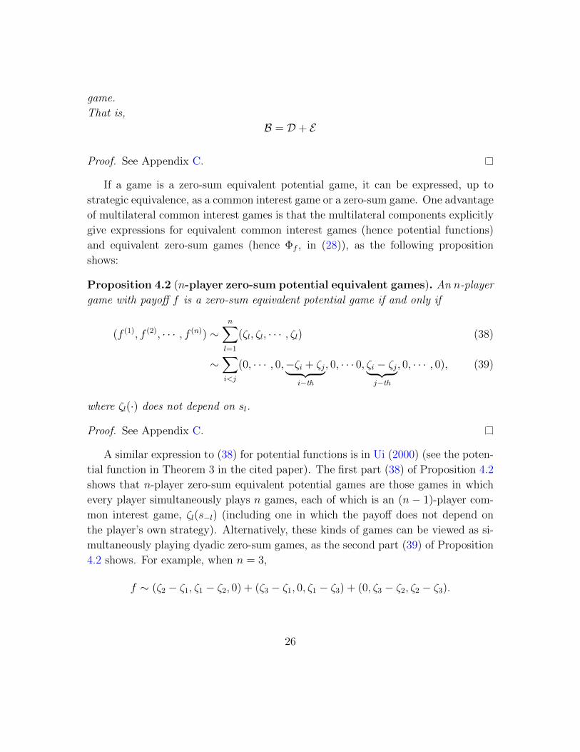
Proposition 4.2 (n-player zero-sum potential equivalent games). An n-player

game with payoff f is a zero-sum equivalent potential game if and only if

(f (1), f (2), · · · , f (n)) ∼n∑l=1

(ζl, ζl, · · · , ζl) (38)

∼∑i<j

(0, · · · , 0,−ζi + ζj︸ ︷︷ ︸i−th

, 0, · · · 0, ζi − ζj︸ ︷︷ ︸j−th

, 0, · · · , 0), (39)

where ζl(·) does not depend on sl.

Proof. See Appendix C.

A similar expression to (38) for potential functions is in Ui (2000) (see the poten-

tial function in Theorem 3 in the cited paper). The first part (38) of Proposition 4.2

shows that n-player zero-sum equivalent potential games are those games in which

every player simultaneously plays n games, each of which is an (n − 1)-player com-

mon interest game, ζl(s−l) (including one in which the payoff does not depend on

the player’s own strategy). Alternatively, these kinds of games can be viewed as si-

multaneously playing dyadic zero-sum games, as the second part (39) of Proposition

4.2 shows. For example, when n = 3,

f ∼ (ζ2 − ζ1, ζ1 − ζ2, 0) + (ζ3 − ζ1, 0, ζ1 − ζ3) + (0, ζ3 − ζ2, ζ2 − ζ3).

26

In the case of n(≥ 3)-player games, because of the externality of strategic interac-

tions, the payoff functions for the dyadic zero-sum games are generally affected by

other players, as well as by those who are directly involved. For example,

(ζ2 − ζ1, ζ1 − ζ2, 0) = (ζ2(s1, s3)− ζ1(s2, s3), ζ1(s2, s3)− ζ2(s1, s3), 0).

Here, the payoff functions for players 1 and 2 are affected by the strategy choices of

player 3, as well as those of players 1 and 2.

4.2. Two-player games

We now turn our attention to two-player games in the class of zero-sum equivalent

potential games. In this case, the n− 1 multilateral common interest games are of

the form (ζ2(s1), ζ1(s2)). That is, a player’s payoff depends only on her own strategy

choices. Thus, an immediate consequence of this observation and Proposition 4.2 is

as follows:

Corollary 4.1 (Two-player zero-sum equivalent potential games). A two-

player game with payoff f = (f (1), f (2)) is a zero-sum equivalent potential game if

and only if

(f (1), f (2)) ∼ (ζ1(s2) + ζ2(s1), ζ1(s2) + ζ2(s1)) (40)

∼ (−ζ1(s2) + ζ2(s1), ζ1(s2)− ζ2(s1)).

Suppose that Condition (R) is satisfied. Then, (s∗1, s∗2) ∈ (arg maxs1 ζ2(s1), arg maxs2 ζ1(s2))

is a Nash equilibrium.

Proof. This immediately follows from Proposition 4.2.

Intuitively, when two players have both common and conflicting interests, the

strategic interdependence effects completely offset each other as in the Prisoner’s

Dilemma game. If we consider a symmetric game in which f (1)(s1, s2) = f (2)(s2, s1)

for all s1, s2 (see footnote 9), condition (40) becomes even stronger:

Corollary 4.2. Suppose that f = (f (1), f (2)) is symmetric; i.e., f (1)(s1, s2) = f (2)(s2, s1)

for all s1, s2. Then, f is a zero-sum equivalent potential game if and only if

f (1)(s1, s2) = ζ1(s2) + ζ2(s1) for some ζ1 and ζ2. (41)

27

Proof. If f is a two-player game, then f ∈ D + E if and only if

f (1)(s1, s2) = ζ1(s2) + ζ2(s1) and f (2)(s1, s2) = ζ ′1(s2) + ζ ′2(s1) (42)

for some ζ1, ζ2 and ζ ′1, ζ′2. Now, if f is symmetric, then clearly (41) holds if and only

if (42) holds.

Using a different approach, Duersch et al. (2012) provide partial results of Corollary

4.2. They show that when a game is a two-player zero-sum game, condition (41)

holds if and only if the game is a potential game. Our result also shows that every

game described by (41) is a zero-sum equivalent potential game. In the context of

population games, Sandholm (2010b) refers to a game strategically equivalent to (41)

as a constant game and shows that a game is a constant game if and only if it is

a potential game with a linear potential function (Proposition 3.2.16 in Sandholm

(2010b)).

In the case of finite games, a stronger characterization than Corollary 4.1 is

possible as follows.

Corollary 4.3. Suppose that a two-player finite zero-sum equivalent potential game

satisfies Condition (N). Then the game has a strictly dominant strategy Nash equi-

librium.

Proof. From the second part of Corollary 4.1, (s∗1, s∗2) ∈ (arg maxs1 ζ2(s1), arg maxs2 ζ1(s2))

is a Nash equilibrium. If there are two distinct maximizers, then since the set of

maximizers is convex, there exist infinitely many Nash equilibria, contradicting Con-

dition (N). Thus, the maximizer is unique and constitutes the strictly dominant

Nash equilibrium.

5. Decomposition of normal form games into components with distinctive

Nash equilibrium characterizations

In this section, we present the decomposition of a given game into components

with different Nash equilibrium characterizations, such as the existence of a com-

pletely mixed strategy equilibrium and a strictly dominant strategy equilibrium.

Before presenting the main results, we show that every normalized zero-sum game

and common interest game possess a uniform mixed strategy Nash equilibrium.

28

Proposition 5.1 (Normalized zero-sum games and normalized common

interest games). Suppose that a game is a normalized zero-sum game or a common

interest game. Then the uniform mixed strategy profile is always a Nash equilibrium.

Proof. Recall from equation (5) that dσi(si) = 1m(Si)

dmi(si) is a uniform mixed

strategy. We define a uniform mixed strategy profile as a product measure of uniform

mixed strategies: i.e.,

dσ(s) =∏i

dσi(si).

Let i and si be fixed. We show that

f (i)(si, σ−i) = 0.

Then, the desired result follows since f (i)(si, σ−i) = 0 = f (i)(σi, σ−i) for all i and si;

hence, f (i)(σi, σ−i) = maxsi f(i)(si, σ−i) for all i. First, by the definition of the mixed

strategy extension,

f (i)(si, σ−i) =

∫s−i∈S−i

f (i)(si, s−i)∏l 6=i

dσl(sl).

If f is a normalized zero-sum game, then

f (i)(si, σ−i) = −∫s−i∈S−i

∑j 6=i

f (j)(sj, s−j)∏l 6=i

dσl(sl) = −∑j 6=i

∫s−i∈S−i

f (j)(sj, s−j)∏l 6=i

dσl(sl) = 0

where the last equality follows from the normalization,∫sl∈Sl

f (l)(sl, s−l)dσl(sl) = 0

for all l and Fubini’s Theorem. If f is a common interest game, then similarly

f (i)(si, σ−i) =

∫s−i∈S−i

v(si, s−i)∏l 6=i

dσl(sl) = 0

where the last equality again follows from the normalization,∫sl∈Sl

v(sl, s−l)dσl(sl) =

0 for all l. Thus, we obtain the desired result.

The immediate consequence of Corollary 3.1 and Proposition 5.1 is that every

two-player finite normalized zero-sum has a unique uniform mixed strategy Nash

equilibrium if Condition (N) holds. If the numbers of two player’s strategies are

29

different, all the normalized zero-sum games and normalized common interest games

always have a continuum of Nash equilibria containing a uniform mixed strategy,

violating Condition (N). The reason is as follows. When the player with a smaller

number of strategies plays the uniform mixed strategy, the other player with a larger

number of strategies has many mixed strategies giving the same expected payoff to

any of the first player’s pure strategies. Thus, all these mixed strategies constitute a

Nash equilibrium, yielding a continuum of Nash equilibria (see a similar discussion

for harmonic games in Candogan et al. (2011)).

Putting all these ingredients together, we obtain the following decomposition of

a given game into components with pure strategy Nash equilibria with a unique

uniform mixed Nash equilibrium and a dominant Nash equilibrium (see Figure 3 for

an illustration of Theorem 5.1).

Theorem 5.1 (Two-player finite strategy games; Nash equilibria). Suppose that f

is a two-player finite strategy game. Then, f can be uniquely decomposed into three

components:

f ∼ fNC + fNZ + fD

where fNC is a normalized common interest game, fNZ is a normalized zero-sum

game, and fD is a zero-sum equivalent potential game. Suppose that all three compo-

nent games satisfy Condition (N). Then, fNC has a finite number of Nash equilibria

with a uniform mixed strategy and fNZ has a unique uniform mixed strategy Nash

equilibrium, and fD a the strictly dominant strategy Nash equilibrium.

Proof. This follows from the decomposition theorem, Theorem 2.1, Corollary 4.3,

and Proposition 5.1.

The bottom line of Figure 3 presents again the decomposition of the symmetric

game in Table 1. In the middle line of Figure 3, we show the Nash equilibria of

the original game and the component games in the simplexes. In the top line we

show the potential function for the normalized common interest game in N ∩ C, the

function Φ for the normalized zero-sum game in N ∩ Z, and the function Φ for the

zero-sum equivalent potential game in B. The decomposition of the game illustrates

how each of the Nash equilibria of the original game is related to the Nash equilibria

of component games. For example, the necessary condition for the existence of the

completely mixed strategy Nash equilibrium for the original game is the existence

of the normalized zero-sum or common interest games. Similarly, the existence of

30

N C N Z B

4,4 -1,1, 1,-1

1, -1 2,2 -2,0

-1,1, 0,-2 2,2

2,2 -1,-1 -1, -1

-1, -1 2,2 -1,-1

-1,-1 -1, -1 2,2

0,0 -1,1 1, -1

1, -1 0,0 -1,1

-1,1 1, -1 0,0

1,1 1,0 1, 0

0, 1 0,0 0,0

0,1 0,0 0,0

∼ ++

(1,0,0)

(0,1,0) (0,0,1)

Potential function functionΦ functionΦ

∼ + +

Figure 3: Decomposition of a game into components with distinctive Nash equilibria.In the bottom line we show the two-player game in Table 1. Since all these games are symmetric,we find all symmetric Nash equilibria for the original games (three pure strategy Nash equilibria,(1, 0, 0), (0, 1, 0), (0, 0, 1), three mixed strategy Nash equilibria involving two strategies (1/2, 1/2, 0),(1/6, 0, 5/6), (0, 2/3, 1/3), and a completely mixed strategy Nash equilibrium (1/6, 1/2, 1/3)) andalso find all symmetric Nash equilibria for all the other component games. We show these Nashequilibria using the simplex in the middle line. The top line shows the potential function and thefunction Φ. The potential function for the zero-sum equivalent potential game in B is given by p1,while the function Φ is given 1− p1, where p = (p1, p2, p3) ∈ ∆.

the pure strategy Nash equilibria, (0, 1, 0) and (0, 0, 1), is due to the existence of the

normalized common interest component. Figure 3 also illustrates that if the effect

of one component is weak (for example, in terms of payoff sizes), then the original

game is expected to be devoid of the desirable properties of the weak component.

Do similar characterizations like Theorem 5.1 extend to two-player continuous

strategy games and n-player games? First, Proposition 5.1 holds for continuous

strategy games. In addition, because of the mini-max characterization for two-player

continuous strategy zero-sum games (Sion’s Theorem), we expect that, under some

conditions, the Nash equilibrium for a zero-sum equivalent game is unique and thus

31

a normalized zero-sum game also has a unique uniform mixed strategy and a zero-

sum equivalent potential game has a strictly dominant strategy (Corollary 4.1). In

fact, using Proposition 3.1, we can provide sufficient conditions for a corresponding

statement for continuous strategy games like Theorem 5.1, which we do not address in

this paper. However, for n-player games, structures of zero-sum equivalent potential

games are complicated as shown in Proposition 4.1. Thus, we do not have a good

answer yet for n-player games and again leave this question to future research.

Finally, since our characterization relies on the linear structure of payoff functions,

it would be useful to know when Nash equilibria remain invariant through linear

combination. The following lemma shows one sufficient condition in such a direction.

Lemma 5.1. Suppose that s∗ is a Nash equilibrium for f and f ′ which have same

strategy sets. Let ρ, ρ′ > 0. Then s∗ is a Nash equilibrium for ρf + ρ′f ′.

Proof. We have

(ρf + ρ′f ′)(i)(s∗i , s∗−i) = ρf (i)(s∗i , s

∗−i) + ρ′(f ′)(i)(s∗i , s

∗−i)

= ρmaxti∈Si

f (i)(ti, s∗−i) + ρ′max

ti∈Si

(f ′)(i)(ti, s∗−i)

= maxti∈Si

ρf (i)(ti, s∗−i) + max

ti∈Si

(ρ′f ′)(i)(ti, s∗−i)

≥ maxti∈Si

(ρf + ρ′f ′)(i)(ti, s∗−i)

Thus, s∗ is a Nash equilibrium.

6. Existing decomposition results

Our decomposition methods extend two kinds of existing results: (i) Kalai and

Kalai (2010), (ii) Hwang and Rey-Bellet (2011); Candogan et al. (2011). First, Kalai

and Kalai (2010) decompose normal form games with incomplete information and

study the implications for Bayesian mechanism designs. Their decomposition is based

on the orthogonal decomposition L = C ⊕ Z in equation (16) in Proposition 2.1.

Second, Hwang and Rey-Bellet (2011) similarly provide decomposition results

based on the orthogonality between common interest and zero-sum games and be-

tween normalized and non-strategic games, mainly focusing on finite games. Cando-

gan et al. (2011) decompose finite strategy games into three components: a potential

32

component, a nonstrategic component, and a harmonic component. When the num-

bers of strategies are the same for all players, harmonic components are the same as

normalized zero-sum games, and their harmonic games, in this case, refer to games

that are strategically equivalent to normalized zero-sum games. Also, their potential

component is obtained by removing the non-strategic component from the potential

part (C + E) of the games. Note that we can change our definition of normalized

zero-sum games to their definition of harmonic games, with all the decomposition

results remaining unchanged. Thus, their three-component decomposition of finite

strategy games follows from Proposition 2.2, (C + E) ⊕ (N ∩ Z) (see the proof of

Corollary 6.1 for more detail).

Corollary 6.1. We have the following decomposition.

L = ((C + E) ∩N )︸ ︷︷ ︸Potential Component

⊕ E︸︷︷︸NonstrategicComponent

⊕ (N ∩ Z)︸ ︷︷ ︸HarmonicComponent

Proof. See Appendix C.

Note that Corollary 6.1 not only reproduces the result of Candogan et al. (2011),

when the number of strategies of the players is the same, but also extends it to the

space of games with continuous strategy sets.

Ui (2000) provides the following characterization for potential games:

f is a potential game if and only if f (i) =∑M⊂NM3i

ξM for some {ξM}M⊂N for all i

(43)

where ξM depends only on sl, with l ∈M . From our decomposition results, we have

D ⊂ C + E and E ⊂ C +D. In particular, the second inclusion holds because

ζi(s−i) =n∑l=1

ζl(s−l)−∑l 6=i

ζl(s−l).

Thus, D ⊂ C+E implies that C+D+E ⊂ C+E and E ⊂ C+D implies C+D+E ⊂C +D. From this, we find

C +D = C +D + E = C + E (44)

33

Note that all games in C and in D satisfy Ui’s condition in (43); hence, games in

C + D satisfy Ui’s condition. Then, equalities in (44) show that the condition in

(43) is a necessary condition for potential games. The sufficiency of Ui’s condition

is deduced by adding the non-strategic game

(∑M⊂NM 631

ξM ,∑M⊂NM 632

ξM , · · · ,∑M⊂NM 63n

ξM)

to game f satisfying Ui’s condition.

Sandholm (2010a) decomposes n-player finite strategy games into 2n components

using an orthogonal projection. When the set of games consists of symmetric games

with l strategies, the orthogonal projection is given by Γ := I − 1l11T , where I is

the l× l identity matrix and 1 is the column vector consisting of all 1’s. Using Γ, we

can, for example, write a given symmetric game, A, as

A = ΓAΓ︸︷︷︸=(N∩C)⊕(N∩Z)

+ (I − Γ)AΓ + ΓA(I − Γ) + (I − Γ)A(I − Γ)︸ ︷︷ ︸=B

. (45)

Thus, our decompositions show that ΓAΓ can be decomposed further into games with

different properties—normalized common interest games and normalized zero-sum

games—and every game belonging to the second component in (45) is strategically

equivalent to both a common interest game and a zero-sum game. Sandholm (2010a)

also shows that a two-player game, (A,B), is potential if and only if ΓAΓ = ΓBΓ. If

P = (P (1), P (2)) is a non-strategic game, it is easy to see that ΓP (1) = O and P (2)Γ =

O, where O is a zero matrix. Thus, the necessity of the condition ΓAΓ = ΓBΓ for

potential games is obtained. Conversely, if ΓAΓ = ΓBΓ, then game (A,B) does not

have a component belonging to N ∩ Z because (ΓAΓ,ΓBΓ) ∈ (N ∩ C) ⊕ (N ∩ Z).

Thus, (A,B) is a potential game.

7. Conclusion

In this study, we developed decomposition methods for classes of games such as

zero-sum equivalent games, zero-sum equivalent potential games, normalized zero-

sum games and normalized common interest games. Our methods rely on the orthog-

onality between common interest and zero-sum games and the orthogonality between

normalized and non-strategic games. Using these, we obtained the first decomposi-

34

tion of an arbitrary game into two components—a zero-sum equivalent component

and a normalized common interest component—and the second decomposition into

three components—a zero-sum equivalent potential component, a normalized zero-

sum component, and a normalized common interest component.

Next, for the class of zero-sum game equivalent games, we showed that each game

in this class has a special function, Φ, whose minima are the Nash equilibria of the

underlying game. Using this function, we showed the convexity of the set of all Nash

equilibria (or the uniqueness of the Nash equilibrium) of a zero-sum equivalent game

under some plausible conditions. In particular, we showed that almost all two-player

finite zero-sum equivalent games have a unique Nash equilibrium. Using decomposi-

tion, we provided characterizations for zero-sum equivalent games. We then studied

the class of zero-sum equivalent potential games and showed that almost all two-

player finite zero-sum equivalent potential games have a unique strictly dominant

Nash equilibrium. We also showed that normalized common interest games and nor-

malized zero-sum games have a uniform mixed strategy Nash equilibrium. Putting

all this together, we showed the decomposition of a two-player finite game into com-

ponent games, each with distinctive Nash equilibrium characterizations (see Figure

3).

35

Appendix

In Appendix A, we recall the basic decomposition results for a Hilbert space. In

Appendix B, we explain in more details our decomposition methods and prove the

related results. In Appendix C, we put other proofs and in Appendix D we compare

the condition for uniqueness in Proposition 3.1 and the condition by Rosen (1965).

A. Decompositions of a Hilbert space

Let L be a Hilbert space with an inner product 〈·, ·〉. First, we recall some elemen-

tary facts about subspaces of the Hilbert space, direct sums, orthogonal projections,

and orthogonal decompositions.

If A and B are subspaces of L, then the sum of A and B, A+ B, is defined as

A+ B := {x+ y ; x ∈ A and y ∈ B},

which is again a subspace of L.

A subspace M is called the direct sum of A and B, A⊕ B, if

(1) M = A+ B.

(2) any z ∈M can be uniquely written as the sum z = x+ y with x ∈ A and y ∈ B.

It is easy to see that M = A⊕ B if and only if M = A+ B and A ∩ B = {0}.In general, given subspaces M and A ⊂ M, there are many choices of B such

that M = A ⊕ B. However, in a Hilbert space, there is a canonical choice of Bconstructed as follows. If A is a subspace of a Hilbert space, L, we denote by A⊥ its

orthogonal complement. That is

A⊥ := {x ∈ L ; 〈x, y〉 = 0 for all y ∈ A} .

Recall that for any subspace A, A⊥ is a closed subspace, and we have A ⊂ A⊥⊥.

Moreover, A = A⊥⊥ if and only if A is a closed subspace of L. A fundamental

theorem in the theory of Hilbert spaces is the following:

Proposition A.1. Let A be a closed subspace of L. Then we have L = A⊕A⊥.

Proof. See, for example, Kreyszig (1989).

36

Related to orthogonal subspaces is the concept of orthogonal projections. An

orthogonal projection, T , is a linear map, T : L → L, which (1) is bounded, (2)

satisfies T 2 = T , and (3) is symmetric (i.e., 〈Tx, y〉 = 〈x, Ty〉) for all x, y ∈ L. Given

an orthogonal decomposition, L = A⊕A⊥, we can define an orthogonal projection,

TA, as

TAz := x if z has the decomposition z = x+ y with x ∈ A, y ∈ A⊥.

Conversely, if T is an orthogonal projection, then from Proposition A.1, one obtains

an orthogonal decomposition

L = kerT ⊕ range(T ) .

Note, that even if two subspaces A, B are closed, A+ B is not always closed.

However, we have the following two lemmas:

Lemma A.1. If A and B are closed orthogonal subspaces, then A⊕ B is closed.

Proof. Consider the orthogonal projections TA and TB. SinceA and B are orthogonal,

we have TATB = 0 and can easily verify that TA + TB is an orthogonal projection

onto A⊕ B, which is then closed.

Lemma A.2. If A is closed and B is finite dimensional, then A+ B is closed.

Proof. Let {zn} be a convergent sequence inA+B (i.e., zn = xn+yn, with xn ∈ A and

yn ∈ B). The sequence {yn} is bounded and by the Bolzano–Weierstrass theorem,

has a convergent subsequence, ynk, which converges to some y in B. Therefore, xnk

is a convergent sequence and, since A is closed, xnkconverges to x ∈ A.

The next two results are crucial to our decomposition theorem.

Lemma A.3. Suppose A and B are subspaces of L. Then,

(i) (A+ B)⊥ = A⊥ ∩ B⊥(ii) If A,B, and A⊥ + B⊥ are closed, then A⊥ + B⊥ = (A ∩ B)⊥.

Proof. Let x ∈ (A + B)⊥. Then, 〈x, y〉 = 0, for all y ∈ A + B. Since A, B ⊂ A + B,we have 〈x, y1〉 = 0, for all y1 ∈ A, and 〈x, y2〉 = 0, for all y2 ∈ B. Thus, (A+B)⊥ ⊂A⊥ ∩ B⊥. Conversely, let x ∈ A⊥ ∩ B⊥ and let y ∈ A+ B. Then, there exist y1 and

y2 such that y1 ∈ A, y2 ∈ B, and y = y1 + y2. Thus, 〈x, y〉 = 〈x, y1〉 + 〈x, y2〉 = 0.

37

Therefore, we have A⊥∩B⊥ ⊂ (A+B)⊥. This proves (i). Then, (ii) is a consequence

of (i): by (i) and sinceA and B are closed, we have (A⊥+B⊥)⊥ = A⊥⊥∩B⊥⊥ = A∩B.

Since A⊥ + B⊥ is closed, we obtain (ii).

Proposition A.2. Suppose that A, B, A+B, and A⊥ +B are all closed subspaces.

Then we have the following decompositions:

(i) L = (A+ B)⊕ (A⊥ ∩ B⊥).

(ii) L = (A⊥ + B)⊕ (A ∩ B⊥).

(iii) L = (A ∩ B⊥)⊕ (A⊥ ∩ B⊥)⊕ ((A+ B) ∩ (A⊥ + B))

Proof. (i) follows from Lemma A.3 (i) and Proposition A.1, since A+ B is assumed

to be closed. (ii) also follows from Lemma A.3 (i) and Proposition A.1, since A⊥+Bis closed and A is closed. For (iii), we first deduce from (i) and (ii) that the subspaces

(A ∩ B⊥) and (A⊥ ∩ B⊥) are closed subspaces. Since they are orthogonal to each

other, by Lemma A.1, the direct sum (A ∩ B⊥)⊕ (A⊥ ∩ B⊥) is also closed. Finally,

by applying Lemma A.3 (i) and (ii) again, we obtain

((A ∩ B⊥)⊕ (A⊥ ∩ B⊥))⊥ = (A ∩ B⊥)⊥ ∩ (A⊥ ∩ B⊥)⊥ = (A⊥ + B) ∩ (A+ B).

Applying Proposition A.1 concludes the proof.

B. Decompositions of the space of games

Recall that the space of games is given by the Hilbert space:

L := L2(S,Rn;m) = {f : S → Rn ; f is measurable and ‖f‖ <∞} .

Note that f ∈ L if and only if f (i) ∈ L2(S,R;m) ={g : S → R ;

∫|g|2dm <∞

}, for

each i = 1, 2, · · · , n. We introduce a number of tools for our decompositions.

Lemma B.1. Let Ti : L2(S,R,m)→ L2(S,R,m) be the map given by

Tig =1

mi(Si)

∫g(s)dmi(si) .

Then, Ti is an orthogonal projection. For i 6= j, Ti and Tj commute, and any product

Ti1Ti2 · · ·Tik is an orthogonal projection.

38

Proof. That T 2i = Ti follows immediately from the definition, and that Ti is sym-

metric follows from Fubini’s theorem. That Ti and Tj commute again follows from

Fubini’s theorem, and a product of commuting projections is always a projection.

Lemma B.2. The following maps are orthogonal projections:

(i) map Λ : L → L, defined by

Λ(f) := (T1f(1), · · ·Tnf (n)) .

(ii) map Φ : L → L, defined by

Φ(f) := (1

n

∑i

f (i), · · · , 1

n

∑i

f (i)).

Proof. (i) follows immediately from Lemma B.1, and (ii) follows from an easy com-

putation.

Corollary B.1. The subspaces C (common interest games), Z (zero-sum games), E(non-strategic games), and N (normalized games) are closed subspaces of L, and we

have

L = C ⊕ Z and L = N ⊕ E .

Proof. We have C = range(Φ), Z = ker(Φ), E = range(Λ), and N = ker(Λ).

Finally, we need the following key proposition:

Proposition B.1. We have the following results:

(i) C + E is closed.

(ii) Z + E is closed.

Proof. For (i), note first that C ∩E is non-empty and contains all constant functions.

For this reason, it will be convenient to treat the constant functions separately. Let

Υ be given by

Υf := (n∏l=1

Tlf(1),

n∏l=1

Tlf(2), · · · ,

n∏l=1

Tlf(n).)

Since Υ and Φ commute, we decompose

C = C0 ⊕ Cconst and E = E0 ⊕ Econst ,

39

where Cconst := range(Υ) ∩ C, C0 := ker(Υ) ∩ C, Econst := range(Υ) ∩ E = range(Υ),

and E0 := ker(Υ) ∩ E . Since Cconst + Econst = Econst , we have

C + E = C0 + E0 + Econst.

Since Econst is finite dimensional, by Lemma A.2, it is now enough to show that C0+E0is closed.

Let {fk}∞k=1 be a convergent sequence in C0 + E0, with limit f = (f (1), · · · , f (2)).

Then, fk = (f(1)k , f

(2)k , · · · , f (n)

k ) has the form

f(i)k = φk + Tig

(i)k ,

for all i, and f(i)k converges to f (i) in L2(S,R;m). We next show that, for every i,

{Tig(i)k }∞k=1 itself is a convergent sequence. Let i be fixed at 1. Since f ∈ C0 + E0, we

have that T1 · · ·Tng(1)k = 0, for all k. Then, we write

T1g(1)k = T1(I − T2)g(1)k + T1T2g

(1)k

= T1(I − T2)g(1)k + T1T2(I − T3)g(1)k + T1T2T3g(1)k

= · · ·

=n∑j=2

(

j−1∏l=1

Tl)(I − Tj)g(1)k , (B.1)

for each k, and we show that each term, {(∏j−1

l=1 Tl)(I−Tj)g(1)k }k, in (B.1) converges.

Since {f (j)k }k converges for all j, so do the differences

f(1)k − f

(j)k = T1g

(1)k − Tig

(j)k −→ f (1) − f (j),

for all j. Then, applying T1(I − T2) to f(1)k − f

(2)k , we see that {T1(I − T2)g

(1)k }k

converges. Applying T1T2(I − T3) to f(1)k − f

(3)k , we see that {T1T2(I − T3)g

(1)k }k

converges and, in general, applying (∏j−1

l=1 Tl)(I − Tj) to f(1)k − f

(j)k , we see that

{(∏j−1

l=1 Tl)(I − Tj)g(1)k }k converges. Thus, every term in (B.1) converges. Therefore,

{T1g(1)k }k converges to some function of the form T1g(1), since range T1 is closed. We

can obviously apply the same argument to Tig(i)k , for all i.

Now, since {f (i)k = φk +Tig

(i)k }k converges and {Tig(i)k }k converges (in range (Ti)),

the sequence {φk} must converge to some φ. Since C0 and E0 are closed, we have

40

(φ, · · · , φ) ∈ C0 and (T1g(1), · · · , Tng(n)) ∈ E0. Therefore, the limit f = (f (1), · · · , f (n))

belongs to C0 + E0, which shows that C0 + E0 is closed.

For (ii), it will be useful to have the following characterization for Z + E :

Claim: f ∈ Z + E if and only if∑n

i=1 f(i) ∈ ker(

∏nl=1(I − Tl)).

Proof of the claim: If f ∈ Z + E , then f (i) = g(i) + h(i), where∑n

i=1 g(i) = 0 and

h(i) ∈ range(Ti). Therefore, we have

n∑i=1

f (i) =n∑i=1

Tiq(i),

for some q(1), · · · , q(n), and clearly, we have (∏n

l=1(I − Tl)) (∑n

i=1 Tiq(i)) = 0.

Conversely, suppose that∑n

i=1 f(i) ∈ ker(

∏nl=1(I − Tl)). Then, we have

f (i) = m(i) + n(i),

where n(i) ∈ ker(∏n

l=1(I − Tl)) and m(i) ∈ range(∏n

l=1(I − Tl)), with∑n

i=1m(i) = 0.

Since ker(∏n

l=1(I − Tl)) = range(T1) + · · ·+ range(Tn), we have, for each i,

n(i) =n∑j=1

Tjn(i)j ,

for some {n(i)j }nj=1. In this way, we find {n(i)

j }i,j. For each i, we write

n(i) =

(n∑j=1

Tjn(i)j −

n∑j=1

Tin(j)i

)+

n∑j=1

Tin(j)i︸ ︷︷ ︸

∈rangeTi

.

Then, we haven∑i=1

(n∑j=1

Tjn(i)j −

n∑j=1

Tin(j)i ) = 0.

This shows that f ∈ Z + E , and concludes the proof of the claim. �Now, suppose {fk}∞k=1 ∈ Z + E , such that fk → f. Then,

∑ni=1 f

(i)k ∈ ker(

∏nl=1(I −

Tl)) and∑n

i=1 f(i)k →

∑ni=1 f

(i). Since ker(∏n

l=1(I − Tl)) is closed in L2(S,R;m),∑ni=1 f

(i) ∈ ker(∏n

l=1(I − Tl)). Thus, f ∈ Z + E .

41

C. Other proofs

Proof of Proposition 3.2. Let F be the set of games that satisfy the condition

given in (34). First, we verify that Z + E ⊂ F . If f ∈ Z, then∑

i f(s) = 0, for all

s, and thus, (34) holds. If f ∈ E and we pick some i ∈ N , then

f (i)(s1, · · · , si−1, ai, si+1, · · · , sn)− f (i)(s1, · · · , si−1, bi, si+1, · · · , sn) = 0

and this holds for any s−i. This implies that

n∑i=1

∑s∈S(a,b)

(−1)#(s)f (i)(s) = 0. (C.1)

Thus, we conclude that Z + E ⊂ F .

To show that F ⊂ Z + E , we show that

F ⊥ (N ∩ C) .

Let f ∈ F satisfy condition (34) and let g ∈ N ∩ C; that is, g = (v, v, · · · , v), with∫v(s)dmi(s) = 0 for every i. Consider ti as fixed and si as varying over Si. Then,

we have, by integrating over si,∫v(s)f (i)(ti, s−i)dmi(si) = f (i)(ti, s−i)

∫v(s)dmi(si) = 0. (C.2)

Now, in condition (34), there are 2n terms involving f (i) and, unless s1 = a1, s2 =

a2 · · · sn = an, f (i) is evaluated as some tj = bj. Thus, if we multiply both sides of

(34) by v(s) and integrate, we find, by (C.1) and Fubini’s theorem,

0 =

∫v(s)

n∑i=1

∑s∈S(a,b)

(−1)#(s)f (i)(s)dm(s)

=

∫v(s)

n∑i=1

f (i)(s1, s2, · · · , sn)dm(s).

However, this simply means that 〈f, g〉 = 0, for f ∈ F and g ∈ N ∩ C. From

Theorem 2.1 (i), we find that (N ∩ C) ⊥ F and F = Z + E .

42

Proof of Corollary 3.2. From (31), if the game is symmetric, then we obtain the

following condition for a zero-sum equivalent game.

f (1)(s1, s2)+f(1)(s2, s1)−f (1)(t1, s2)−f (1)(s2, t1)−f (1)(s1, t2)−f (1)(t2, s1)+f

(1)(t1, t2)+f(1)(t2, t1) = 0

(C.3)

If we set s = s1 = s2 and t = t1 = t2, then equation (C.3) implies condition in (35).

Now suppose that condition in (35) holds. Then we have

f (1)(s, s) + f (1)(t, t) = f (1)(s, t) + f (1)(t, s)

and thus

f (1)(s1, s2) + f (1)(s2, s1)− f (1)(t1, s2)− f (1)(s2, t1)

− f (1)(s1, t2)− f (1)(t2, s1) + f (1)(t1, t2) + f (1)(t2, t1)

=f (1)(s1, s1) + f (1)(s2, s2)− f (1)(t1, t1)− f (1)(s2, s2)

− f (1)(s1, s1)− f (1)(t2, t2) + f (1)(t1, t1) + f (1)(t2, t2)

=0

and thus (C.3) holds.

Proof of Proposition 3.3. Let i and l be fixed, and suppose that

f (i)(s) =1

ml(Sl)

∫f (i)(sl, s−l)dml.

If l = i, then f = (0, · · · , f (i)(s)︸ ︷︷ ︸i−th

, · · · , 0), which is a passive game and, hence, is

strategically equivalent to a zero-sum game. Thus, suppose that l 6= i. Consider a

component, (0, · · · ,−f (i)(s)︸ ︷︷ ︸l−th

, · · · , 0). Then, this component is again a passive game.

In this way, for all i, we can define a passive game such that the sum of f and all

resulting passive games is zero. Thus, f is strategically equivalent to a zero-sum

game.

43

Proof of Proposition 3.4. Recall that

π(i)((s1, · · · , sk), (sk+1, · · · , s2k)) =

{∑2kl=k+1 f

(1)(si, sl, τ(i)1 , τ

(l)2 )piql if i ≤ k∑k

l=1 f(2)(sl, si, τ

(l)1 , τ

(i)2 )plqi if i ≥ k + 1

.

(C.4)

Then from Proposition ..., π is strategically equivalent to a zero-sum game. Suppose

that (f (1)(sα, sβ, τ1, τ2), f(2)(sα, sβ, τ1, τ2)) is a potential game, for each τ1 and τ2. Let

i and l be fixed. Without loss of generality, i ≤ k and l ≥ k + 1. Consider

(0, · · · , f (1)(si, sl, τ(i)1 , τ

(l)2 )piql︸ ︷︷ ︸

i−th

, 0, · · · , 0, f (2)(sl, si, τ(l)1 , τ

(i)2 )plqi︸ ︷︷ ︸

j−th

, 0 · · · , 0). (C.5)

Since (f (1), f (2)) is a potential game, (f (1), f (2)) ∼ (g, g), for some g. Then,

(g(si, sl), g(si, sl), · · · , g(si, sl), 0︸︷︷︸i−th

, g(si, sl), · · · , g(si, sl), 0︸︷︷︸j−th

, g(si, sl), · · · )

is a passive game. Thus, the component in (C.5) is a potential game. Similarly,

we can show that other components are potential games, which shows that π is a

potential game.

Proof of Proposition 4.1. We first show that

B = (Z + E) ∩ (C + E) = Φ(Λ(L)) + E .

Let f ∈ (Z+E)∩(C+E). Then, f = g1+h1, for g1 ∈ Z and h1 ∈ E , and f = g2+h2,

for g2 ∈ C and h2 ∈ E . Thus, we have

g1 + h1 = g2 + h2, (C.6)

and applying Φ to (C.6), we obtain

f = Φ(h1 − h2) + h2.

Thus, since h1 − h2 ∈ Λ(L), f ∈ Φ(Λ(L)) + E . Conversely, let f ∈ Φ(Λ(L)) + E .

44

Obviously, f ∈ C + E . In addition, f = Φ(Λ(g)) + h1, for g ∈ L and h1 ∈ E . Thus,

f = Φ(Λ(g)) + h1 = −(I − Φ)(Λ(g)) + Λ(g) + h1 ∈ Z + E .

This shows that

(Z + E) ∩ (C + E) = Φ(Λ(g)) + E .

Note that

Φ(Λ(L)) + E={f : f (i) =n∑l=1

ζl(s−l) for some {ζl}nl=1 and for all i}+ E

= {f : f (i) =∑l 6=i

ζl(s−l) for some {ζl}nl=1 and for all i}+ E

= D + E .

Proof of Proposition 4.2. Observe that

(∑l 6=1

gl(s−l),∑l 6=2

gl(s−l), · · · ,∑l 6=n

gl(s−l))

∼ (n∑l=1

gl(s−l),n∑l=2

gl(s−l), · · · ,n∑l=1

gl(s−l)).

Hence, the first result follows from D+E = (C+E)∩ (Z +E). For the second result,

45

observe that

(∑l 6=1

gl,∑l 6=2

gl, · · · ,∑l 6=n

gl) ∼ (∑l 6=1

gl − (n− 1)g1,∑l 6=2

gl − (n− 1)g2, · · · ,∑l 6=n

gl − (n− 1)gn)

= (∑l 6=1

(gl − g1),∑l 6=2

(gl − g2), · · · ,∑l 6=n

(gl − gn))

= (∑l>1

(gl − g1), g1 − g2, g1 − g3, · · · , g1 − gn)

+ (0,∑l>2

(gl − g2), g2 − g3, · · · , g2 − gn) + · · ·

+ (0, 0, · · · ,∑l>n−1

(gl − gn−1), gn−1 − gn)

=n∑i=1

n∑l>i

(0, · · · , 0,−gi + gj︸ ︷︷ ︸i−th

, 0, · · · 0, gi − gj︸ ︷︷ ︸j−th

, 0, · · · , 0).

Proof of Corollary 6.1. This proof follows from Proposition 2.2 by showing that

((C + E) ∩N )⊕ E = C + E . First, observe that (C + E) ∩N ⊂ C + E , which implies

that ((C + E) ∩ N ) ⊕ E ⊂ C + E . Now, let f ∈ C + E . Then, f = g + h, where

g ∈ C, h ∈ E , and g = (v, v, · · · , v). Then, by applying the map, Λ, we find that

f = Λ(f) + (I −Λ)(f). Obviously, Λ(f) ∈ E . In addition, (I −Λ)(f) = (I −Λ)(g) =

(v − T1v, v − T2v, · · · , v − Tnv) ∈ C + E . Thus, (I − Λ)(f) ∈ (C + E) ∩N .

D. Comparison of the condition for uniqueness in Proposition 3.1 and the

condition by Rosen (1965)

To simplify we consider the two player zero-sum equivalent game given by

f (1)(s1, s2) = w(1)(s1, s2) + h(1)(s2)

f (2)(s1, s2) = w(2)(s1, s2) + h(2)(s1)

and suppose that w(1) and w(2) are differentiable. Then Proposition 3.1 (ii) requires

that∂2w(1)

∂s21< 0 and

∂2w(1)

∂s22> 0.

46

Also, the sufficient condition for the uniqueness of the Nash equilibrium for concave

games by Rosen (1965) (Theorems 2 and 6) is given by(2r1

∂2w(1)

∂s21r1

∂2w(1)

∂s1∂s2+ r2

∂2w(2)

∂s1∂s2

r1∂2w(1)

∂s1∂s2+ r2

∂2w(2)

∂s1∂s22r2

∂2w(2)

∂s22

)=

(2r1

∂2w(1)

∂s21r1

∂2w(1)

∂s1∂s2− r2 ∂

2w(1)

∂s1∂s2

r1∂2w(1)

∂s1∂s2− r2 ∂

2w(1)

∂s1∂s2−2r2

∂2w(1)

∂s22

)

is negative definite for some r1, r2 > 0. Thus Rosen’s condition requires some re-

striction on the cross partial derivatives, while the condition in Proposition 3.1 does

not.

47

Bibliography

Barron, E. N., 2008. Game Theory: An Introduction. Wiley.

Bregman, L. M., Fokin, I. N., 1998. On separable non-cooperative zero-sum games.

Optimization 44 (1), 69–84.

Cai, Y., Candogan, O., Daskalakis, C., Papadimitriou, C., 2015. A multiplayer gen-

eralization of the minmax theorem. Mathematics of Operation Research, Forth-

coming.

Candogan, O., Menache, I., Ozdaglar, A., Parrilo, P. A., 2011. Flows and decom-

positions of games: Harmonic and potential games. Mathemtics of Operations

Research 36 (3), 474–503.

Cornes, R., Hartley, R., 2005. Asymmetric contests with general technologies. Eco-

nomic Theory 26, 923–946.

Duersch, P., Oechssler, J., Schipper, B. C., 2012. Pure strategy equilibria in symmet-

ric two-player zero-sum games. Internation Journal of Game Theory 41, 553–564.

Hino, Y., 2011. An improved algorithm for detecting potential games. International

Journal of Game Theory 40, 199–205.

Hofbauer, J., Schlag, K., 2000. Sophisticated imitation in cyclic games. Journal of

Evolutionary Economics.

Hofbauer, J., Sigmund, K., 1998. Evolutionary Games and Population Dynamics.

Cambridge Univ. Press, Cambridge.

Hwang, S.-H., Rey-Bellet, L., 2011. Decomposition of two player games: Potential,

zero-sum, and stable games. arXiv:1106.3552.

Hwang, S.-H., Rey-Bellet, L., 2015. Simple characterization of potential games and

zero-sum games, 2015.

Kalai, A., Kalai, E., 2010. Cooperation and competition in strategic games with

private information. EC ’10 Proceedings of the 11th ACM conference on Electronic

commerce.

48

Konrad, K. A., 2009. Strategy and Dynamics in Contests. Oxford University Press,

Oxford.

Kreyszig, E., 1989. Introductory Functional Analysis with Applications. Wiley.

Monderer, D., Shapley, L. S., 1996. Potential games. Games and Economic Behavior

14, 124–143.

Morris, S., Ui, T., 2004. Best response equivalence. Games and Economic Behavior

49, 260–287.

Myerson, R. B., 1997. Dual reduction and elementary games. Games and Economic

Behavior 21, 183–202.

Osborne, M. J., Rubinstein, A., 1994. A Course in Game Theory. MIT Press.

Rosen, J. B., 1965. Existence and uniqueness of equilibrium points for concave n-

person games. Econometrica 33 (3), 520–534.

Sandholm, W., 2010a. Decompositions and potentials for normal form games. Games

and Economic Behavior 70, 446–456.

Sandholm, W., 2010b. Population Games and Evolutionary Dynamics. MIT Press.

Savani, R., von Stengel, B., 2006. Hard-to-solve bimatrix games. Econometrica 74 (2),

397–429.

Szidarovszky, F., Okuguchi, K., 1997. On the existence and uniqueness of equilibrium

in rent-seeking games. Games and Economic Behavior 18, 135–140.

Ui, T., 2000. A Shapley value representation of potential games. Games and Eco-

nomic Behavior 31, 121–135.

Ui, T., 2009. Bayesian potentials and information structures: Team decision problems

revisited. Internation Journal of Game Theory 5, 271–291.

Weibull, J., 1995. Evolutionary Games Theory. Cambridge, MA.

Wilson, R., 1971. Computing equilibria of n-person games. SIAM Journal of Applied

Mathematics 21 (1), 80–87.

49

Wu, W.-T., Jiang, J.-H., 1962. Essential equilibrium of points of n-person non-

cooperative games. Scientia Sinica 11, 1307–1322.

Zeeman, E., 1980. Population dynamics from game theory. Global Theory of Dy-

namical Systems 819.

50