Embed Size (px)
Citation preview

LUND UNIVERSITY
PO Box 117221 00 Lund+46 46-222 00 00
Stored energies in electric and magnetic current densities for small antennas
Jonsson, B.L.G.; Gustafsson, Mats
2014
Link to publication
Citation for published version (APA):Jonsson, B. L. G., & Gustafsson, M. (2014). Stored energies in electric and magnetic current densities for smallantennas. (Technical Report LUTEDX/(TEAT-7234)/1-38/(2014); Vol. TEAT-7234). [Publisher informationmissing].
Total number of authors:2
General rightsUnless other specific re-use rights are stated the following general rights apply:Copyright and moral rights for the publications made accessible in the public portal are retained by the authorsand/or other copyright owners and it is a condition of accessing publications that users recognise and abide by thelegal requirements associated with these rights. • Users may download and print one copy of any publication from the public portal for the purpose of private studyor research. • You may not further distribute the material or use it for any profit-making activity or commercial gain • You may freely distribute the URL identifying the publication in the public portal
Read more about Creative commons licenses: https://creativecommons.org/licenses/Take down policyIf you believe that this document breaches copyright please contact us providing details, and we will removeaccess to the work immediately and investigate your claim.
Download date: 03. Jan. 2022
Electromagnetic TheoryDepartment of Electrical and Information TechnologyLund UniversitySweden
CODEN:LUTEDX/(TEAT-7234)/1-38/(2014)
Stored energies in electric andmagnetic current densities forsmall antennas
B.L.G. Jonsson and Mats Gustafsson

B.L.G. [email protected]
Royal Institute of TechnologySchool of Electric EngineeringTeknikringen 33SE-100 44 StockholmSweden
Mats [email protected]
Department of Electrical and Information TechnologyElectromagnetic TheoryLund UniversityP.O. Box 118SE-221 00 LundSweden
Editor: Gerhard Kristenssonc© B.L.G. Jonsson and Mats Gustafsson, Lund, November 14, 2014

1
Abstract
Electric and magnetic currents are essential to describe electromagnetic stored
energy, as well as the associated quantities of antenna Q and the partial di-
rectivity to antenna Q-ratio, D/Q, for general structures. The upper bound
of previous D/Q-results for antennas modeled by electric currents is accu-
rate enough to be predictive, this motivates us here to extend the analysis
to include magnetic currents. In the present paper we investigate antenna
Q bounds and D/Q-bounds for the combination of electric- and magnetic-
currents, in the limit of electrically small antennas. This investigation is both
analytical and numerical, and we illustrate how the bounds depend on the
shape of the antenna. We show that the antenna Q can be associated with the
largest eigenvalue of certain combinations of the electric and magnetic polariz-
ability tensors. The results are a fully compatible extension of the electric only
currents, which come as a special case. The here proposed method for antenna
Q provides the minimum Q-value, and it also yields families of minimizers for
optimal electric and magnetic currents that can lend insight into the antenna
design.
1 Introduction
Time harmonic electromagnetic radiating systems do not in general have a nitetotal energy associated with them. This is well known since the radiated electricand magnetic elds decay as r−1 and the corresponding energy density hence decayas r−2, which is not an integrable quantity for exterior unbounded regions. This non-integrability diers from the singularities of the electromagnetic energy for chargedparticles, see e.g., [14, 69], where the challenge is the nite mass of particles incoupling Maxwell's equation to the dynamics of the charged particles.
To consistently extract a nite stored energy from the energy densities associ-ated with classical time-harmonic energy has been investigated in [10, 11, 18, 32, 58,62, 68]. These stored energies have been based on spherical (and spheroidal) modes,circuit equivalents and on the input impedance for small antennas. In 2010 Vanden-bosh [63] proposed a current-density approach to stored energies also applicable tolarger antennas. This approach has generated new interest in electromagnetic storedenergy that is explored in [8, 24, 27, 28, 64, 65]. This `stored energy' is similar to theresults of Collin and Rothschild [11] and it also has similarities with the stored ener-gies proposed in [9, 20]. The generalization in [66] and in the present paper includeselectric and magnetic current-densities for arbitrary shapes. Antennas embedded inlossy or dispersive material has been considered in [29].
The drive to nd a well-dened stored energy stems partly from that it is closelyrelated to the antenna quality factor Q. Lower bounds on antenna Q is directlyrelated to the electric size of the antenna, and indirectly to the maximal matchingbandwidth that can be obtained. The relation between antenna Q and bandwidthis not trivial, for a discussion and examples see e.g., [22, 23, 28, 68]. An alternativemethod to derive bandwidth bounds is sum-rules, see e.g., [15, 25, 37, 40, 52, 68].The approach given here, is related to [25, 27, 28, 66, 68]. In the present paper, we

2
show how the electric and magnetic polarizabilities [42, 54, 55] are directly relatedto lower bounds on antenna Q for small antennas. The investigation is based on theasymptotic behavior of stored energy in the electrically small case for both electricand magnetic currents. This result is an extension of the stored energies in [63] andtheir connection to both antenna Q and partial directivity over antenna Q. Thatscattering properties are related to the polarizabilities are known, see e.g. [5, 60],but that polarizability tensors appear directly as the essential factor in antennaQ-estimates is a recent result [25, 38, 66, 67].
The current-representation approach to stored energy enables the maximal par-tial directivity over antenna Q problem to be reduced to a convex optimizationproblem [24]. It also enables us to consider fundamental limitations for arbitrarygeometries. Convex optimization problems are eciently solvable [7]. From a userperspective it can be compared with solving a matrix equation. To numerically ndthe physical bounds on antenna Q or partial directivity over antenna Q, D/Q ishere reduced to tractable problems, solvable with common electromagnetic tools.In the present paper we illustrate how this can be applied to a range of shapes,both numerically and analytically. The here considered minimization problems in-vestigate how dierent current and charge density combinations yield dierent lowerbounds on antenna Q. For the electrical dipole problem we show that the minimiz-ing currents result in Q and D/Q that agree with [25, 62, 67]. For the case of ageneralized electric dipole with both electric charges and magnetic current-densitiesas sources our result agrees with the sphere in [10]. When we allow dual-modes,i.e., both electrically and magnetically radiation dipoles, we nd that the resultagree with [38, 66]. The framework here easily account for all these dierent caseswith a generic approach. Another result of our method is that we can show thatsmall antennas have a family of current-densities that realize the associated optimalantenna Q for a given shape [27].
The present paper is based on the stored energies for both electric and magneticcurrent densities [38]. Another approach to these energies and associated boundsare given in [66]. We investigate the small antenna limit and illustrate how antennaQ and related optimization problems behave for electric and magnetic currents fora range of antenna shapes. These results are based on the leading order termsof the stored energies as the electric size of the domain approach zero. One of theadvantages here is that the bounds on Q and D/Q are known once the polarizabilitytensors are determined for a given shape. We use this knowledge to sweep shape-parameters to illustrate how Q andD/Q depend on the shape of antenna. Analyticalexpressions for the electrically small case provide physical insight into limiting factorsfor Q and D/Q. These more general results are shown to reduce to the analyticallyknown cases in [26, 66, 67].
In Section 2, we recall the denitions of key antenna and energy quantities.Using an asymptotic expansion of the electric and magnetic currents in Section 3 wegive the explicit leading order current-density representation of the radiated power,stored energies, and the radiation intensities. Analytical and numerical examples forantenna Q and D/Q under dierent constraints are given in Section 4. In Section 5,we formulate the problem as a convex optimization problem, and determine Q for

3
Je,Jm, ρe, ρm
an
V∂V
Figure 1: The gure illustrates the joint support, V , of the current densities,enclosed within a sphere of radius a, and with a normal n at the boundary ∂V ofV .
some shapes. Conclusions and appendices end the paper.
2 Antenna Q and partial directivity
Let V ⊂ R3 be the joint bounded support of the electric and magnetic currentdensities Je and Jm respectively, see Figure 1. The support V is here assumed to bebounded and connected. Through the continuity equations we dene the associatedelectric and magnetic charge densities ρe and ρm. The time-harmonic Maxwell'sequations with electric and magnetic current densities in free-space take the form
∇×E + jηkH = −Jm, ∇ ·E =ρe
ε=−ηjk∇ · Je, (2.1)
∇×H − jk
ηE = Je, ∇ ·H =
ρm
µ=−1
jkη∇ · Jm, (2.2)
where we use the time convention ejωt, which is suppressed. In this paper, we letε = ε0, µ = µ0 and η = η0 =
√µ/ε be the free space permittivity, permeability and
impedance, respectively. E is the electric eld and H is the magnetic eld. Thedispersion relation between the wave number, k, and the angular frequency, ω, isk = ω
√εµ and t is time.
The eld energy densities are ε|E|2/4 and µ|H|2/4. Here we are interested instored electric We and magnetic Wm energies, which are more challenging to dene.We follow the denition of [11, 16, 20, 22, 28, 63, 68] and dene the stored electric andmagnetic energies as
We =ε
4
∫R3r
|E(r)|2 − |FE(r)|2r2
dV, Wm =µ
4
∫R3r
|H(r)|2 − |FH(r)|2r2
dV, (2.3)
where FE,FH are the far-elds, i.e., E → FEe−jkr
ras r → ∞ and ηFH = r × FE.
Let r denote a vector in R3, with length r = |r| and corresponding unit vectorr = r/r. Here
∫R3ris an abbreviation of the limit limr0→∞
∫|r|<r0 . Note that the

4
expressions (2.3) can for certain antennas become coordinate dependent, and forlarge structures (2.3) may become negative [27], these artifacts do not appear in thesmall electrical limit, as shown later in this paper as all obtained minimal antennaQ are non-negative, see e.g., Section 4.
Given these stored energies, we dene the two main antenna parameters thatappear in the physical bounds. The antenna quality factor: Q = max(Qe, Qm, 0)where
Qe =2ωWe
Prad
, and Qm =2ωWm
Prad
. (2.4)
Here, Prad is the radiated power of the system described by (2.1)-(2.2). Dened as
Prad =1
2η
∫Ω
|FE(r)|2 dΩ, (2.5)
where Ω is the unit sphere in R3.The partial directivity D(k, e) in the direction k from an antenna with polar-
ization e, is [3]
D(k, e) = 4πP (k, e)
Prad
, (2.6)
where P (k, e) is the partial radiation intensity |e · FE|2/(2η). The other mainantenna parameter here is the partial directivity over antenna Q, D/Q, which withthe above notation is
D(k, e)
Q=
2πP (k, e)
ωmax(We,Wm, 0). (2.7)
The goal here is to optimize and investigate Q and D/Q in terms of the electricand magnetic current densities, in the small antenna limit. We hence express thesequantities in terms of the current densities, see A. While these calculations arestraight forward, they are also rather lengthy, see e.g., [63] for a similar eort, seealso [38, 39]. Substantial simplication is obtained in these derivations for the caseof electrically small antennas which is illustrated in the next section. The leadingorder term of the stored energies, for small k is given by
We =µ
4kIm[〈Je,LeJe〉+
1
η2〈Jm,LmJm〉
]+O(k) (2.8)
and
Wm =µ
4kIm[〈Je,LmJe〉+
1
η2〈Jm,LmJm〉
]+O(k). (2.9)
Note that these stored energies are symmetric in the current densities and a naturalextension of the electric only current-case, Jm = 0. Above we use the ordo notationO(k) to indicate that the next order term is bounded by Ck, for some constant Cas k → 0. The associated operators in (2.8) and (2.9) are
〈J ,LeJ〉 =−1
jk
∫V
∫V
∇1 · J(r1)∇2 · J∗(r2)G(r1 − r2) dV1 dV2, (2.10)
〈J ,LmJ〉 = jk
∫V
∫V
J(r1) · J∗(r2)G(r1 − r2) dV1 dV2. (2.11)

5
The operators are similar to the Electric Field Integral Equation, EFIE, operatorsL = Le−Lm, when the currents are on a surface of an object, and for such currentsthere is a range of implementations in the standard method-of-moment codes. Hereand below we occasionally use the notation `current', in place of `current density',to shorten the notation. The kernel G(r) is the Green's function, e−jkr/(4πr) and ∗indicates the complex conjugate, see also Figure 1.
The radiation intensity, P (k) in the direction k, have a representation in termsof the current densities [38]:
P (k) =ηk2
32π2
[∣∣ ∫V
(e∗ · Je(r1) +1
ηk × e∗ · Jm(r1))ejkr·r1 dV1
∣∣2+∣∣ ∫V
(h∗ · Je(r1) +1
ηk × h∗ · Jm(r1))ejkr·r1 dV1
∣∣2] = P (k, e) + P (k, h), (2.12)
where we use that k, e, h is an orthogonal triplet with k× e = h. We recognize thepartial radiation intensity P (k, e) for the polarization e. For electric currents only,i.e., Jm = 0, these expression agree with e.g., [27, 63].
To nd the total radiated power Prad, in terms of its current-density representa-tion we can integrate (2.12) over the unit sphere. A more direct route to Prad is basedon (2.5) and the observation that the electric far-eld, FE, have the representation
FE(r) =jηk
4πr ×
∫V
[r × Je(r1) +
1
ηJm(r1)
]ejkr·r1 dV1. (2.13)
Somewhat lengthy calculations [38, 39] show that the corresponding quadratic formin terms of the currents are
Prad =η
2Re〈Je,LJe〉+
1
2ηRe〈Jm,LJm〉 − Im〈Je,K1Jm〉, (2.14)
where K1 is the operator dened by
〈Je,K1Jm〉 =k2
4π
∫V
∫V
J∗e (r1) · R× Jm(r2)j1(kR) dV1 dV2. (2.15)
Here R = r1 − r2, R = |R|, R = R/R and jn(x) is the spherical Bessel function oforder n [1].
The small electrical size limit simplify the above energy and power related ex-pressions We,Wm, P (k) and Prad and subsequently Q and D/Q. We utilize that theradius, a, of the enclosing sphere, is electrically small, i.e., that ka is small enoughto motivate that we discard higher order terms. To expand the above quantities interms of small ka we assume that the currents have the asymptotic behavior:
Je = J (0)e + kJ (1)
e +O(k2) with ∇ · J (0)e = 0, (2.16)
Jm = J (0)m + kJ (1)
m +O(k2) with ∇ · J (0)m = 0. (2.17)
This assumption is consistent with the continuity equations for the electric andmagnetic current densities. Note that J
(0)e , J
(0)m , J
(1)m and J
(1)m are all k-independent
and the two latter correspond to a lowest order static charge through the continuityequation.

6
3 Electrically small volume approximation
We apply the small ka approximation and (2.16), (2.17) to the partial radiationintensity and the far-eld FE in the form of (2.13). We rst note that∫
V
Jejkk·r dV =
∫V
J (0) + kJ (1) + jk(k · r)J (0) +O(k2) dV
= −jk
∫V
jJ (1) +1
2k × (r × J (0)) dV +O(k2), (3.1)
where we have used that [59, p432]:∫V
J (n)e,m dV =
0, n = 0,
−∫Vr∇ · J (n)
e,m dV, n 6= 0,(3.2)
and [59, p433], [43, p127]∫V
(k · r)J (0)e,m dV =
−1
2k ×
∫V
r × J (0)e,m dV, (3.3)
since ∇ · J (0)e,m = 0. Here J
(n)e,m, indicate that the expression is valid for J
(n)e and
J(n)m , n = 0, 1. It follows that the partial radiation intensity (2.12), for a wave with
polarization e and propagating in direction k is P (k, e) = P (0)(k, e)+O(k5), whereP (0) reduces to
P (0)(k, e) =ηk4
32π2
∣∣ ∫V
e∗ · (jJ (1)e +
1
2ηr× J (0)
m ) + k× e∗ · ( j
ηJ (1)
m −1
2r× J (0)
e ) dV∣∣2
=ηk4
32π2
∣∣e∗ · πe + k × e∗ · πm
∣∣2. (3.4)
Here we used that the triplet k, e∗, h∗ forms an orthogonal basis system. The
πe =
∫V
jJ (1)e +
1
2ηr × J (0)
m dV and πm =
∫V
j
ηJ (1)
m −1
2r × J (0)
e dV (3.5)
terms are generalized dipole-moments that account for both the electric and mag-netic dipole radiating elds, respectively.
To nd the total radiated power in (2.5) we start with inserting the expansion(3.1) into the far-eld (2.13) to nd the small ka approximation of the far-eld:
FE(k) =ηk2
4πk×
∫V
k×(jJ (1)e +
1
2ηr×J (0)
m )+(j
ηJ (1)
m −1
2r×J (0)
e ) dV +O(k3). (3.6)
We insert (3.6) into the expression for the total radiated power (2.5), to nd that

7
Prad = P(0)rad +O(k5) where
P(0)rad =
ηk4
32π2
∫Ω
|πe|2 − |k · πe|2 + |πm|2 − |k · πm|2 − 2k · Re(πm × π∗e ) dΩ
=ηk4
12π(|πe|2 + |πm|2)
=ηk4
12π
∣∣∣ ∫V
jJ (1)e +
1
2ηr × J (0)
m dV∣∣∣2 +
∣∣∣ ∫V
j
ηJ (1)
m −1
2r × J (0)
e dV∣∣∣2 = Pe + Pm.
(3.7)
Here we used the integration over the unit sphere Ω of the angular variables in kto nd the relations
∫Ωk dΩ = 0 and
∫Ω|k · πe|2 dΩ = 4π
3|πe|2. The radiated power
consists of two types of terms: terms that radiate as electric dipoles with power Pe
and the second part that radiates as magnetic dipoles with power Pm. An alternativederivation to calculate Prad in the small volume limit is to start from (2.14), see C.The power in terms of the dipole-moments can alternatively be expressed as
Prad =k4
12π√εµ
[∣∣ 1√εpe −
√εmm
∣∣2 +∣∣ 1√µpm +
õme
∣∣2]+O(k5), (3.8)
where jcpe =∫VJ
(1)e dV andme = 1
2
∫Vr×J (0)
e dV and analogously for the magneticcurrents and moments with subscript m, i.e., mm. Here c = 1/
√εµ is the speed of
light.A check that the above expressions agree with what is known for small antennas
that radiate as dipoles is obtained by comparing the maximal partial directivity,i.e., P (0)(k, e) to the total radiation Prad. We consider two cases: xed generalizedelectric dipole moments and no generalized magnetic dipole moment (3.5) i.e., πm =0 and πe 6= 0 (or vice versa) and xed non-zero πm,πe:
maxe
4πP (0)(k, e)
P(0)rad
=3
2, when πm = 0, (3.9)
and
maxe,e⊥k
4πP (0)(k, e)
P(0)rad
= maxe,e⊥k
3
2
|e∗ · (πe − k × πm)|2|πe|2 + |πm|2
≤ 3. (3.10)
Stating that a small antenna with electric dipole radiation from a generalized elec-tric dipole moment have directivity 3/2, but upon adding a magnetic generalizeddipole πm we nd that appropriate oriented combinations of πe and πm can have adirectivity of 3, corresponding to a Huygens source see e.g., [51].
The small electric volume stored energies follow directly from their integral rep-resentation (2.8), we nd that We = W
(0)e +O(k), where
W (0)e =
µ
16π
∫V
∫V
[ 1
η2J (0)
m (r1) ·J (0)∗m (r2)+(∇1 ·J (1)
e (r1))(∇2 ·J (1)∗e (r2))
] 1
R12
dV1 dV2
(3.11)

8
and similarly (2.9) yields Wm = W(0)m +O(k), where
W (0)m =
µ
16π
∫V
∫V
[J (0)
e (r1)·J (0)∗e (r2)+
1
η2(∇1 ·J (1)
m (r1))(∇2 ·J (1)∗m (r2))
] 1
R12
dV1 dV2.
(3.12)
4 Minimal antenna Q and analytical and
numerical illustrations
One of the goals with the above expressions for antenna Q and D/Q is that theyshould lend us some insight into antenna design and limitations of Q and D/Q. It isreasonable to ask the question of what shapes that give low antenna Q. Similarly weinvestigate which charge and current densities that gives low antenna Q. Anothergoal with the expressions is to nd easily derived a priori bounds of antenna Q andD/Q. Partial answers are given in this section, that extends the relation that alarge charge-separation ability in the domain imply a small antenna Q see e.g., [2527, 66, 67]. Similarly we may think of a shape with low antenna Q, as a structurethat supports a large `current loop area' for a magnetic dipole-moment. One of thenew results here is that the generic shape results in [27] for D/Q is extended tolower bounds on antenna Q.
An often studied case is the electric-dipole case [2426, 63, 67], here representedby the electric charges only and we illustrate below how an optimization problemis used to determine the minimal Q. We continue and show that the method andits associated eigenvalue-problem extend to the more general case of both electricand magnetic currents that radiate as an electrical dipole. Here we also nd thatthe magnetic polarizability enters in the lower bounds on Q. A short review ofpolarizability tensors are given in B.
Consider the minimization problem for nding the lower bound on Q.
Q = minimizeρ(1)e ,ρ
(1)m ,J
(0)e ,J
(0)m
2ωmaxW (0)e (ρ
(1)e ,J
(0)m ),W
(0)m (ρ
(1)m ,J
(0)e ), 0
Pe(ρ(1)e ,J
(0)m ) + Pm(ρ
(1)m ,J
(0)e )
, (4.1)
with the two constraints∫Vρ
(1)e dV = 0 and
∫Vρ
(1)m dV = 0. Here jωρ
(1)e = −k∇·J (1)
e
and similarly for ρ(1)m . One of the interesting cases in antenna design is when the
antenna radiate as an electrical dipole, i.e., when Pm is negligible and Wm ≤ We.Once the optimal (Pe,We) is determined we tune the antenna with a tuning circuitto make the antenna resonant, i.e., Wm = We. Thus we start with the optimizationproblem for a pure (We, Pe)-case. The `dual mode' case, where both Pe and Pm
are comparable is considered in Section 4.4 below. Before we consider the generalcase, let's start with the easier case of an electric dipole when we have only ρe, i.e.,J
(0)m = 0.

9
4.1 Antenna Q for an electric dipole, e.g., Pm = 0
Dierent approaches to lower bounds of this antenna Q case has also been inves-tigated in e.g., [2427, 63, 64, 67]. However, one of the goals here is to arrive toa generic method that works for dierent cases of current-density sources, and therst step towards this goal, is to verify that this method indeed gives the previouslyderived result on the lower bound see e.g., [25, 27, 62, 66, 67]. The electric dipoleis here equivalent with the assumption Pm = 0 and We ≥ Wm which yields thatQ = Qe and that we have an optimization problem that depend only on the electriccharge-densities ρe. Once the design is determined we can tune the antenna with atuning circuit to make We = Wm. This case is the classical electrical dipole-case.Let ρe = ρ
(1)e . The minimization problem (4.1) reduces to:
Qe = minimizeρe
2ωW 0e (ρe)
Pe(ρe)=
6π
k3minimize
ρe
∫V
∫Vρ∗e (r1)ρe(r2)4π|r1−r2| dV1 dV2
|∫Vrρe dV |2 , (4.2)
where we have used (3.2) to re-write the denominator. This minimization comes withthe constraint that no current ows through the surface ∂V , i.e., 0 =
∫∂Vn ·Je dS =
−jc∫Vρe dV , where c is the speed of light. Hence, (4.2) is accompanied with the
constraint of total zero charge,∫Vρe dV = 0.
The associate problem to maximize D/Q in the small electric volume limit forarbitrary ρe, see [27] corresponds to:
D
Qe
= maximizeρe
2πP 0(k, e)
ωW 0e (ρe)
=k3
4π
|∫Ve∗ · rρe(r) dV |2∫
V
∫Vρ∗e (r1)ρe(r2)4π|r1−r2| dV1 dV2
, (4.3)
with the same constraint of a total zero charge,∫Vρe dV = 0. These two problems
are related but the D/Q-problem has the simplication in that the integrand inP 0(k, e) see (3.4), is scalar-valued and the maximization has a convex optimizationformulation see [24, 27].
The method that we apply below to (4.2) works on both problems (4.2) and (4.3)and yield the same result as in [27] where it is applied to (4.3). The nal result issimilar to the result in [66, 67], but obtained with dierent methods. Note that both(4.2) and (4.3) remain unchanged under the scaling, ρ 7→ αρ. Thus the solutionsto (4.2) are a family of scaling invariant solutions. We determine the minimum bybreaking the scaling-invariance by selecting a particular value of the amplitude ofthe dipole moment, pe. We rewrite (4.2) as the minimization problem as:
minimizeρe
∫V
∫V
ρ∗e(r1)ρe(r2)
4π|r1 − r2|dV1 dV2, (4.4)
subject to |∫V
rρe(r) dV |2 = p2e, (4.5)∫
V
ρe(r) dV = 0. (4.6)
This is a classical optimization problem for the Newton-potential. An energy spaceapproach in a similar context is discussed in [44] and an approach that allow for

10
geometries with corners is given in [33]. We note that there may be several minimiz-ers that realize the same minimum, e.g., for spheres and shapes with appropriatesymmetries [55]. To explicitly nd the minimum, we use the method of Lagrangemultipliers see e.g., [70, 4.14] and dene the Lagrangian Q as
Q(ρ, ρ∗, λ1, λ2) =
∫V
∫V
ρ∗(r1)ρ(r2)
4π|r1 − r2|dV1 dV2 − λ1(|
∫V
rρ dV |2 − p2e)− λ2
∫V
ρ∗ dV.
(4.7)Here λ1 and λ2 are Lagrange multipliers, and we use the short hand notation ρ = ρe.Variation of Q with respect to λ1 and λ2 gives the two constraints above. Takingthe variation of Q with respect to ρ∗, or equivalently, taking a Fréchet derivative ofQ yields the Euler-Lagrange equation for the critical points∫
V
(1
4π|r1 − r2|− λ1r1 · r2
)ρ(r1) dV1 = λ2, r2 ∈ V. (4.8)
Note that this is an integral equation with unknown ρ. Accompanied with theconstraints we nd three equations (4.8), (4.5), and (4.6) and three unknown ρ, λ1
and λ2.Upon multiplying (4.8) with ρ∗ and integration over V , utilizing the zero total
charge constraint, we nd that Qe in (4.2) is equivalent with
Qe =6π
k3minρλ1. (4.9)
The unknown Lagrange multiplier, λ1, depends implicitly on ρ and λ2. The lowerbound of the minimization problem (4.2) is hence determined by the unknown La-grange multiplier λ1, times a constant. Another property of the solution appears ifwe apply Laplace operator on (4.8), for r /∈ ∂V we have that ρ(r) = 0. Thus wereduce (4.8) to:∫
∂V
(1
4π|r1 − r2|− λ1r1 · r2
)ρs(r1) dS1 = λ2, r2 ∈ ∂V, (4.10)
where ρs is the surface charge density, i.e., we have formally the relation that ρ dV =ρs dS. A similar result for D/Q was shown in [27].
Using the constraint |∫∂Vrρs dS| = pe > 0 we re-write the critical equation (4.10)
into: ∫∂V
ρs(r1)
4π|r2 − r1|dS1 = λ1pep · r2 + λ2, r2 ∈ ∂V (4.11)
for some unknown unit vector p.To solve the equation (4.11) we make rst a few observations: Any solution ρs
of (4.11) for given right hand-sides, yields an associated potential that solves anelectrostatic boundary-value problem cf., B. Such solutions are restricted in theirasymptotic behavior by the electric polarizability tensor γe, which depends only onthe shape of V . To make this restriction explicit we note that the electric polariz-ability tensor γe is dened through (B.2) and (B.4): γe · eD0 = p. Comparing (B.2)

11
with (4.11), we see that the generic D0e in (B.2) is here D0e = λ1pep, and thedipole-moment is by denition p =
∫∂Vrρs dS. Since the electric polarizability ten-
sor γe is given, once the shape V is known, we thus have a constraint on (λ1, p) inorder for ρs and its associated potential to comply with the polarizability tensor.The constraint is that:
γe · p =1
λ1
p, (4.12)
which we recognize as a eigenvalue problem in (λ1, p) for γe. Here we have usedthat p = pep.
We conclude that critical points of (4.2) correspond to solutions (λ1, p) of theeigenvalue problem (4.12). Given such a solution (λ1, p) we determine the associ-ated charge-density through (4.11) with (λ1, p) given as solutions to (4.12). A chargedensity that solves (4.11) is hence the base for the family of current-sources that sup-ports the optimal radiation, which we obtain from the continuity equation. Throughthe re-writing of the optimal Qe in (4.9) it follows that the largest eigenvalue, (γe)3
of the polarizability matrix γe yields the minimum Qe, i.e.,
Qe =6π
k3(γe)3
. (4.13)
We have hence reduced the variational problem of nding the minimum Qe forthe electric dipole to nding eigenvalues of γe. This result have large similaritiesto [66, 67], derived with dierent methods. We conclude thatQk3 in the small volumesize only depend on shape and size as expressed through the electric polarizability.The physical interpretation connects large polarizability eigenvalues to the ability ofthe structure to separate charge under an external static eld in a given direction.The polarizability γe is associated with the scalar Dirichlet-problem of the Laplaceoperator, and depend only on the shape of the object [54]. We note also that γe isidentical with the high-contrast electric polarizability in e.g., [25].
We note that the low-frequency magnetic charge density and electric chargedensity antenna Q are dual-similar, and hence if we consider a case with either a ρe-term or a ρm-terms both of these problems result in identical minimization problemswith a lower bound on antenna Q given by (4.13).
To compare with the D/Q-problem, we note that the constraint |∫e∗ ·rρs dV | =
const, was in [27] reduced to∫e · rρ∗s dV = α, yielding the critical equation corre-
sponding to (4.11) as∫∂V
ρs(r1)
4π|r1 − r2|dS1 = ν1e · r2 + ν2, r2 ∈ ∂V. (4.14)
Similarly to Qe-case above we nd that ν1 is connected to γe through the relatione∗ · γe · e = α
ν1. The corresponding maximum is D/Q = k3
4πe∗ · γe · e. We thus
see that the two problems are related, but that they describe dierent optimizationproblems. The antenna Q lower bound, minimize Q without concern of radiationdirection of the antenna, whereas D/Q assume a xed e radiation direction thoughout its optimization. With a-priori knowledge about the optimal radiation directionof the structure or alternatively the principal eigenvalue of γe associated with a

12
given structure, we select e in this direction, to nd the expected 3/2 dierencebetween 1/Qe and D/Qe. This D/Q result is similar to the sum-rule in [25] forelectric sources. With the Qe result and the observation of principal directions ofγe we see that these three approaches illustrate closely connected results here witha common energy principle method to obtain them.
To illustrate the result we begin with a sphere: γe = 4πa3I, where I is the 3times 3 unit tensor, and all eigenvalues of γe are identical. Note that to these de-generate eigenvalues there are three orthogonal eigenvectors, and the correspondingcharge densities in (4.10) for each a given amplitude of the dipole-moment pe. Thisdegeneracy is due to the geometrical symmetries of the shape. Thus even when weremove the scaling invariance, we may have multiple ρ that yields the same lowerbound on Q. Note also that for any arbitrary optimizer ρe = ρ
(1)e that the associ-
ated electric current connected to ρ(1)e , here J
(1)e , i.e., jωρ
(1)e = −∇ · J (1)
e , has aninnite dimensional subspace that all yield the same ρ
(1)e . It allows a potentially
large design-freedom that does not change Qe in the quasi-static limit. This case isanalogous to the case discussed in [27].
For the sphere we nd (ka)3Qe = 32and for a disc (ka)3Qe = 9π
8for the electrical
dipole case, see D. If we instead study γe of a rectangular plate of size `2 × `1 andsweep the ratio `1/`2 we nd that the two non-zero eigenvalues depicted as the twocurves with highest value (red, green) in Figure 2a, and corresponding Q in Figure 2bmarked with (E). Note thatD/Q = k3e∗·γe·e/4π, and hence proportional to the twoelectric polarizability curves given in Figure 2a, for given direction e. The electricalpolarizability here can physically be thought of as how well a structure allow chargeseparation, in the sense that large eigenvalues in a direction correspond to largestatic electric dipole-moment, or equivalently large ability to separate charges.
The corresponding, electric charge maximization problem ofD/Q is solved in [2527]. We have thus the solution to both the minρQ and the maxρD/Q problems forsmall antennas for small antennas that radiate as electric dipoles.
4.2 Antenna Q for an electric current magnetic dipole
Analogous to how the electric dipole, ρ(1)e , and the magnetic dipole with ρ
(1)m yield
the same optimization problem in the previous section, we see that an electric J(0)e
or a magnetic J(0)m current density result in identical optimization problems. We
associate a magnetic dipole momentm = mm an electric current density, J(0)e here
denoted J , to nd the minimization problem:
Qm = minimizeJ
W(0)m (J)
Pm(J)= minimize
J
6π
k3
∫V
∫V
J∗(r1)·J(r2)4π|r1−r2| dV1 dV2∣∣ ∫
V12r × J dV
∣∣2 , (4.15)
with the constraint that n · J = 0 over the surface and J ∈ X0, as dened in (B.5)see Section 4.3 and B for a more detailed discussion of this choice. This problemis associated with an antenna that radiates as a magnetic dipole i.e., Pe = 0, andWe ≤ Wm. Once the optimization is done we can tune the antenna with a tuningcircuit to reach resonance We = Wm.
13
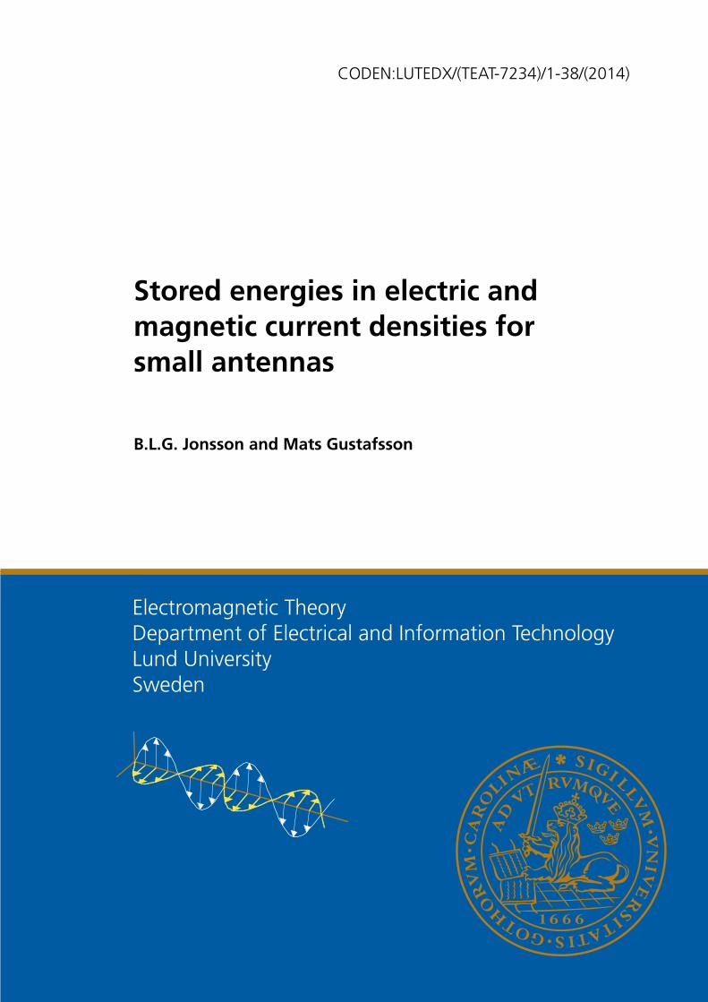
100 101 10210−3
10−2
10−1
100
`1/`2
(γe) 1
1,(γe) 2
2,(γm) 3
3/
a3
a
`2
`1
(E)e
(E) e
(M)h
(a)100 101 102
101
102
103
104
`1/`2
(ka)3Q
e,Q
m
a
`2
`1
(E)
(M)
(b)
Figure 2: (a) Eigenvalues for the electric and magnetic polarizability for an in-nitesimally thin plate normalized by a3, where a = (
√`2
1 + `22)/2 is the radius of a
circumscribed sphere. The polarization directions are indicated by e and h for theE and H-elds respectively. The curves are marked with (E) for electric polariz-ability or (M) for magnetic polarizability. The curves are symmetric with respect to`1/`2 = 1, the lowest curve is the single non-zero eigenvalue of γm. (b) The corre-sponding Q-value from (4.13), (4.21), once again the (E) correspond to the electricand (M) to the magnetic case.
We apply once again the method in (4.2)(4.7) to the minimization of (4.15).Scaling invariance is broken by the assumption that |1
2
∫Vr × J dV | = m, which
reduces the problem (4.15) to an equivalent problem with Lagrange multipliers.The Lagrangian is
Q(J ,J∗, λ1) =
∫V
∫V
J∗(r1) · J(r2)
4π|r1 − r2|dV1 dV2 − λ1(
∣∣ ∫V
1
2r × J dV
∣∣2 −m2) (4.16)
for J ∈ X0, see (B.5). The associated critical point equation is∫V
J(r2)
4π|r1 − r2|dV2 = −λ1
2r1 ×
∫V
1
2r2 × J(r2) dV2 = −λ1m
2r1 × m. (4.17)
Similar to the electric case (4.9) we take the scalar product of (4.17) with J∗ andintegrate over V to nd that Qm is determined by λ1.
Qm =6π
k3minJλ1. (4.18)
By applying the operator∇×∇× to (4.17), we realize that the currents have supportonly on the boundary, i.e., J dV = Js dS, and the equation (4.17) reduce to
n×∫∂V
Js(r2)
4π|r1 − r2|dS2 =
λ1m
2n× (m× r1), for r1 ∈ ∂V, (4.19)
where n is normal to ∂V .Similarly to the electric case (4.11), we compare this with the denition of the
magnetic polarizability tensor, γm in (B.6) and (B.10): γm · hH0 = m. The mag-netic polarizability tensor is known, once the region V is given. The (λ1, m) in

14
equation (4.19) is hence subject to constraint:
γm · m =1
λ1
m. (4.20)
The eigenvalue solution (λ1, m) of (4.20) yields the solution to the minimizationproblem:
Qm =6π
k3minJλ1 =
6π
k3(γm)3
, (4.21)
where (γm)3 is the largest eigenvalue of γm. The analogous case for D/Q is givenin [27]. The sphere has magnetic polarizability 2πa3I, which yields (ka)3Qm = 3cf., [51, 62]. Here I is a unit 3 times 3 tensor.
The electric and magnetic polarizabilities of a rectangular plate are depictedin Figure 2a marked with (E) and (M) respectively. The polarizability tensor arediagonal for geometries with two orthogonal reection symmetries and co-alignedcoordinate system [42, 48] and for planar structures we have only one eigenvalueof γm, orthogonal to the plane. We can physically think of large γm-eigenvaluesas that the region V support a large loop current for the corresponding dipole-moment. Note that planar structures have one non-zero eigenvalue in γm which isassociated to the normal-to-the-surface dipole-moment with the planar `current looparea'. We observe that the magnetic polarizability tensor is connected to the scalarNeumann-problem of Laplace equation, see B, and is hence the second of the two`rst-moment' (or dipole) quantities associated with a given shape. Note that themagnetic polarizability correspond to the permeable case of µ → 0. There are dif-ferent sign conventions for γm, however we note that λ1 ≥ 0 in (4.21) independentlyof choice of sign-convention in the denition of γm, see (4.15).
A similar current loop-area argument is illustrated in Figure 3, for a at ellipseand a thin ellipsoid. The eigenvalues of the polarizability tensor of an ellipsoid areknown, see D, and they are depicted in Figure 3ab. The two curves marked with(M) in Figure 3c correspond to Qm, the upper one (blue) is for an ellipse of zerothickness and only one γm-eigenvalue corresponding to a current loop-area over thesurface. The other marked (M,thick) corresponds to an ellipsoid identical to theat one, but where the radius normal to the paper is h/100 where h is the heightof the ellipse. The two transverse eigenvalues of γm are ignored by Qm until thewidth, w, is h/100, where equivalent current loop-area of the height-normal (out ofthe paper) loop dominates the transverse current loop-area and Qm changes slowlyfor w/h < 10−2 since this area is essentially preserved.
4.3 Lower bound on antenna Q for both electric charge and
magnetic currents
The common electric and magnetic dipoles cases above agree with previously derivedresults [28, 66]. We here extend these results to include both the electric chargedensity ρe and the magnetic current density Jm i.e., the components making up ageneralized electric dipole-moment πe (3.5). We once again consider the case where

15
10−3 10−2 10−1 100
10−5
10−2
101
ee
e
ξ = w/h
γe/a3
10−4
10−2
100 (M)
h
h
h
γm/a
3
10−3 10−2 10−1 100100
101
102
103
104
105
(M)(E,E+M)
(E+M,thick)
(M,thick)(M)
ξ = w/h
(ka)3Q
e,Q
m,Q
a
h
w
ah
w
ah
w
(a) (c)
(b)
Figure 3: (a) Eigenvalues to the electric polarizability tensor, γe. Solid lines are theat-case, dashed lines correspond to the case with normal (out of the paper) radiusof the ellipsoidal is h/100. Polarization direction is indicated with an arrow. (b)Eigenvalues to the magnetic polarizability tensor γm. Solid line correspond to theat case, dashed lines are the case with normal radius h/100. Note that the x-axisis the same as in (a). (c) The antenna Q for a at ellipse indicated by (E), and (M)and (E+M) corresponding to Qe from electric sources (4.13), Qm from magneticsources (4.21) and, Q from combined dual-mode in (4.34) respectively. Two linesare also marked with `thick', to indicate that the ellipsoidal radius normal to theellipse-surface in the gure is h/100. Note in particular for Qm, that as the widthbecomes smaller than h/100, the thickness become important, as is clear in (4.21),since it implies a switch of dominant eigenvalue. The reduction of Q as comparedto Qe due to the eigenvalue of γm is absent for at structures since the non-zeroeigenvalues of γe and γm have orthogonal directions. It is a marginal reduction forstructures with small thickness. See also D.
the antenna radiates as an electrical dipole, i.e., Pm = 0 and where the storedenergy is mainly electric, Wm ≤ We. After the optimization we tune the antenna tomake the stored electric and magnetic energies equal. Optimizing for the (Pm,Wm)-case is identical to the (Pe,We)-case up to a sign and the free-space impedancenormalization of the currents. Similar to the above discussion in Section 4.1 andSection 4.2 of electric and magnetic dipoles we optimize
Q =6π
k3minρ,J
∫V
∫Vρ∗(r1)ρ(r2)+J∗(r1)·J(r2)
4π|r1−r2| dV1 dV2∣∣ ∫Vrρ− 1
2r × J dV
∣∣2 . (4.22)
We above use the short hand notation J = J(0)m /η, and ρ = cρ
(1)e = j∇·J (1)
e . Here wealso have the constraints
∫Vρ dV = 0 and that ∇ · J = 0 to account for the Gauge-
freedom of the associated vector-potential. To include this Gauge-freedom into theoptimization problem we restrict the current-density space to J ∈ X0, see (B.5).
The minimization problem is scaling invariant under transformations (ρ,J) 7→

16
(ρ,J)α for any complex valued scalar α. By assuming that the denominator has agiven value π2
e , we may equivalently consider the problem
minimizeρ,J
∫V
∫V
ρ∗(r1)ρ(r2) + J∗(r1) · J(r2)
4π|r1 − r2|dV1 dV2, (4.23)
subject to∣∣ ∫
V
rρ(r)− 1
2r × J(r) dV
∣∣2 = π2e , (4.24)∫
V
ρ∗(r) dV = 0, (4.25)
J ∈ X0. (4.26)
Using the method of Lagrange multipliers λ1, λ2, we dene the Lagrangian
Q =
∫V
∫V
ρ∗(r1)ρ(r2) + J∗(r1) · J(r2)
4π|r1 − r2|dV1 dV2
− λ1(∣∣ ∫
V
rρ− 1
2r × J dV
∣∣2 − π2e )− λ2
∫V
ρ∗ dV. (4.27)
Critical points of Q are determined by the variation (Fréchet derivative) of Q. Vari-ation with respect to the Lagrange parameters λ1 and λ2 gives the constraints. Thevariation with respect to ρ∗ and J∗ yields:∫
V
ρ(r2)
4π|r1 − r2|dV2 = λ1
[r1 ·
∫V
r2ρ(r2)− 1
2r2 × J(r2) dV2
]+ λ2, (4.28)∫
V
J(r2)
4π|r1 − r2|dV2 =
λ1
2r1 ×
∫V
r2ρ(r2)− 1
2r2 × J(r2) dV2. (4.29)
Here we utilized that n · J = 0 on ∂V , and we recognize λ2 as a way to ensurethat the total charge is zero. To investigate the properties of these Euler-Lagrangeequations, we rst note that the inner product of these equations with ρ∗ and J∗
respectively and that their sum can be rewritten as the original problem:
Q =6π
k3minρ,J
∫V
∫Vρ∗(r1)ρ(r2)+J∗(r1)·J(r2)
4π|r1−r2| dV1 dV2∣∣ ∫Vrρ− 1
2r × J dV
∣∣2 =6π
k3minρ,J
λ1. (4.30)
The minimization problem is thus reduced to nding λ1 for ρ,J that solves (4.28)and (4.29).
Similar to the charge-density case (4.9), we note that λ1 implicitly depend on ρand J through the Euler-Lagrange equations. Another property of the minimizationproblem appears if we for r /∈ ∂V operate with ∆ and with ∇ × ∇× on (4.28)and (4.29) respectively. We nd that ρ and J only have support on the boundary,and we use the notation J dV = Js dS and ρ dV = ρs dS. We hence nd the

17
Euler-Lagrange equations∫∂V
ρs(r2)
4π|r1 − r2|dS2 = λ1(r1 ·
∫∂V
r2ρs(r2)− 1
2r2 × Js(r2) dS2) + λ2
= −λ1r1 · πe + λ2, (4.31)
n1 ×∫∂V
Js(r2)
4π|r1 − r2|dS2 = λ1n1 × (
1
2r1 ×
∫∂V
r2ρs(r2)− 1
2r2 × Js(r2) dS2)
= −λ1n1 × (1
2r1 × πe), (4.32)
for r1 ∈ ∂V . We have here introduced the electric and magnetic dipole-momentsfor the current and charge-distribution that solve (4.31) and (4.32): p =
∫∂Vrρs dS,
m = 12
∫∂Vr × Js dS and πe = m − p. However both m and p are presently
unknown apart from the constraints that |πe| = |p−m| = πe.To determine λ1, we recall the denitions of the electric polarizability tensor γe
and magnetic polarizability tensor γm in B. We compare (4.31) and (4.32) with(B.2) and (B.6). The polarizability tensors γe and γm are known, once V is given,and we nd that (B.4) and (B.10) impose constraints on λ1 and πe:
γe · (p−m) =1
λ1
p, γm · (p−m) =−1
λ1
m. (4.33)
Adding the two equations yields that λ−11 is an eigenvalue to the matrix γe + γm.
Furthermore, m − p = πeπe, where πe is an eigenvector of γe + γm of unit length.Thus we have found that in this case the lower bound on Q is given by
Q =6π
k3(γe + γm)3
, (4.34)
where (γe +γm)3 is the largest eigenvalue of the γe +γm tensor. The correspondingρs,Js are hence the solution of (4.31) and (4.32), where m− p = πeπe, i.e., in thedirection of the unit eigenvector corresponding to the largest eigenvalue. This resultis similar to [66], but derived with a dierent method. Note that γe + γm ≥ 0.
The minimization procedure also establish that there exists a λ1 ≥ 0 such that∣∣ ∫V
rρ− 1
2r × J dV
∣∣2 ≤ 1
λ1
∫V
∫V
ρ∗(r1)ρ(r2) + J∗(r1) · J(r2)
4π|r1 − r2|dV1 dV2 (4.35)
for all ρ and J that satisfy the bi-condition J ∈ X0 and∫Vρ dV = 0. Equality is
reached when ρ and J satisfy the Euler-Lagrange equations above, yielding 1/λ1 =(γe + γm)3. An equivalent formulation of this result is
Pe ≤ (γe + γm)3ck4
3πWe, or Pm ≤ (γe + γm)3
ck4
3πWm, (4.36)
for the above described currents. The identity is achieved in either case for currentsthat realize the minimization of Qe or Qm. The inequality for the (Pm,Wm)-case isobtained identically with above described case starting from Pm and Wm with thesubstitution of J = −J (1)
e and ρ = cρ(1)m /η giving (4.22) with rρ + r × J/2 of the
integrand in the denominator.

18
4.3.1 Comparisons and numerical examples for the Q-lower bound for
the dual-mode case (4.34)
0 0.2 0.4 0.6 0.8 10
0.2
0.4
0.6
0.8
1
ζ = min(d, h)/max(d, h)
γe/(4πa3)
0
0.2
0.4
γm/(4πa3)
0 0.2 0.4 0.6 0.8 1
100
101
102
ζ = min(d, h)/min(d, h)(ka)3Q
e,Q
m,Q,Q
tot
(a) (c)
(b)
h
d
h
h
h
h
e
e
ee
(T)
(+)
(E)
(M)
Figure 4: (a) Eigenvalues for the electric polarizability tensor. Polarization di-rection is indicated with a vertical or horizontal arrow. (b) Eigenvalues of themagnetic polarizability tensor. The x-axis is the same as the axis in (a). (c)Qe from (4.13) is marked with (E), Qm from (4.21) marked with (M) and Qfrom (4.34) are marked with a (+) and for the dual-mode antenna (4.39) witha (T). Note that the (γe)11 = 2(γm)33, as for axial-symmetric objects shownin [48]. Dashed lines in (abc) are the prolate case, solid lines are the oblate case.(ka)3(Qm, Qe, Q+, QT )→ (3, 3/2, 1, 1/2) as ζ → 1 i.e., the sphere. See D.
We note that for a sphere where both electric and magnetic currents contributeto the generalized electric dipole-moment we nd that (ka)3Qe = 1 [10]. The Q-lower bound for the at ellipse and the thin ellipsoid are depicted in Figure 3. Forplanar structures we note that there is only one non-zero eigenvalue of γm, in thedirection normal to the surface and hence perpendicular to the non-zero directionof γe. For a rectangular plate this eigenvalue is depicted in Figure 2. We concludethat in planar structures γe and γm do not couple to improve the antenna Q. As isclear from the case where we add a small thickness of the domain as in Figure 3c,we see that there is a rather small reduction of Q as compared with the at case.
The polarizability tensors for spheroidal shapes are known, see D and Figure 4ab.We depict Q for spheroidal bodies as a function of the ratio between height anddiameter in Figure 4c. Here, the curve marked with (+) correspond to Q givenin (4.34) are shown for both the prolate (dashed lines) and oblate cases (solid lines).
The approach in [67] provides an antenna Q, QV , depending only on γe andvolume V . To compare QV with (4.34) we use the inequality [54, 1.5.19]:
(e·γe ·e−V )(e·γm ·e−V ) ≥ V 2 ⇔ (e·γe ·e−V )(e·(γe+γm)·e) ≥ (e·γe ·e)2. (4.37)

19
Rewriting and comparing with the results we nd that
Q =6π
k3e · (γe + γm) · e ≤6π
k3e · γe · e(1− V
e · γe · e) = QV , (4.38)
if we choose the e to be the unit eigenvectors corresponding to the largest eigenvalueof γe + γm. Equality holds for several cases in particular for ellipsoidal-shapes. Anupdated approach to antenna Q is given in [66], see also [38]. To illustrate thatthere is a dierence between Q and QV we calculate both antenna Q's for a cylinder.We assume here that the currents radiate as an electrical dipole aligned with thecylinder axis, i.e., the vertical x3-axis, the resulting Q from (4.34) and QV areshown in Figure 5. To demand that a small antenna radiates as an electric dipolein a given direction is equivalent with selecting the corresponding eigenvalue of thepolarizability tensor. Such a choice of eigenvalue does not necessarily minimizeantenna Q.
10-3
10-2
1 10 102
103
0
5
10
15
20
0.1
Qk a33
Je
Jm
J +Je m
` /`1 2
`1
`2
`2
`1
Figure 5: The gure depicts the antenna Q, for energies that corresponds to cur-rents that radiate as an electrical dipole aligned with the vertical axis. The dottedgreen line correspond to QV in (4.38), the Je, Jm and Je + Jm correspond to Qe,Qm and Q in respectively (4.13), (4.21) and (4.34).
The above examples illustrate how the shape of a small antenna enters intothe antenna Q-bound. The shape characterization in antenna Q is encoded in therespective polarizability tensors. The electric polarizability is a measure on howeasy it is to separate charge for a given V , i.e., to create a large electric dipole-moment. Similarly, the magnetic polarizability measure how easy it is to create alarge magnetic dipole moment, i.e., nding a large `current-loop area' in the domain.
If we similarly to [30, 61, 66] associate the magnetic currents with layers/volumesof magnetization or synthesized Amperian current loops we note that the associatedvolumes for the electric and magnetic currents do not necessary need to occupy

20
identical volumes/surfaces. In such a case there are a considerable design freedomfor γe and γm, with the performance bounded by the eigenvalues of γe + γm for thetotal volume V .
4.4 Dual mode antennas
Self-resonant dual mode-antennas where both the electric Pe and magnetic Pm dipoleradiation contribute signicantly to the radiation and We = Wm is considered here.Utilizing that the problem decouples, we use the respective electric and magneticcase above with identities (4.35) where λ1 ≥ 0 for both We and Wm. We hence ndthat the general case can be bounded by:
Q ≥ 6π
k3
max(We,Wm)
λ−11 We + λ−1
1 Wm
≥ 6π
k3
λ1
2=
3π
k3(γe + γm)3
, (4.39)
which follows directly from the Hölder inequality [46]. Equality follows when bothelectric and magnetic charges are optimized and the antenna is self-resonant. Clearlywe nd that Q is half the value of Qe or Qm when only electric or magnetic dipoleradiation is allowed. The sphere yields (ka)3Q = 1/2, which agrees with the resultof the sphere given in [10, 31, 47]. A similar result is given in [66], derived with adierent method1. The antenna Q for this case is illustrated for spheroidal shapesin Figure 4c, for curves marked with a (T).
5 Convex optimization for optimal currents
Bounds on D/Q can be expressed as a convex optimization problems [24]. Here,these results are generalized to include electric and magnetic current densities. Weconsider a volume V with electric Je and magnetic Jm current densities. We expandthe current densities in local basis-functions
Je(r) ≈N∑n=1
Je,nψn(r) and Jm(r) ≈N∑n=1
Jm,nψn(r) (5.1)
and introduce the 1 × 2N matrix Jv with elements Je,n for n = 1, ..., N andη−1Jm,n−N for n = N + 1, ..., 2N to simplify the notation. The basis functionsare assumed to be real valued, divergence conforming, and having vanishing normalcomponents at the boundary [50].
A standard method of moment implementation using the Galerkin procedurecomputes the stored energies given in A as matrices. For simplicity, we here computethese stored energy matrices Xe and Xm only for the leading order term in (2.10)and (2.11), for ka 1, i.e.,
Xeij =
1
k
∫V
∫V
∇1 ·ψi(r1)∇2 ·ψj(r2)cos(kR12)
4πR12
dV1 dV2 (5.2)
1Optimization that utilize a xed electric to magnetic dipole radiation ratio is discussed in [66].
21
and
Xmij = k
∫V
∫V
ψi(r1) ·ψj(r2)cos(kR12)
4πR12
dV1 dV2. (5.3)
The quadratic forms for the stored energies (2.8) and (2.9) are then approximatedas
We ≈η
4ωJH
v XeJv =η
4ω
N∑i,j=1
J∗e,iXeijJe,j + J∗m,iX
mij Jm,j (5.4)
and
Wm ≈η
4ωJH
v XmJv =η
4ω
N∑i,j=1
J∗e,iXmij Je,j + J∗m,iX
eijJm,j. (5.5)
where the superscript, H, denotes the Hermitian transpose.We also use the radiated far eld, FE(r) see (3.6). The radiation vector projected
on e, cf., (3.6), denes the 2N × 1 matrix E∞ from
e∗ · FE(k) ≈ E∞Jv
= −jηkN∑n=1
[Je,n
∫V
e∗ ·ψn(r)ejkk·r
4πdV + Jm,n
∫V
k × e∗ ·ψn(r)ejkk·r
4πdV], (5.6)
Using the scaling invariance of D/Q, we rewrite the maximization of D/Q intothe convex optimization problem of maximization of the far-eld in one directionsubject to a bounded stored energy [24], i.e.,
maximizeJv
ReE∞Jv,
subject to JH
v XeJv ≤ 1,
JH
v XmJv ≤ 1.
(5.7)
The formulation is easily generalized by adding additional convex constraints [24].There are several ecient implementations that solve convex optimization problems,here we use CVX [21].
We consider planar geometries and bodies of revolution to illustrate the bound.The resulting Q of (2.4) for a small spherical capped dipole antenna is depictedin Figure 6a as a function of the angle θ for a maximized omnidirectional partialdirectivity in θ = 90 and polarized in the z-direction. The resulting radiationpattern is as from a z-directed electric Hertzian dipole, i.e., D = 1.5 sin2 θ. Thethree cases; electric and magnetic currents Je + Jm, only electric currents Je, andonly magnetic currents Jm are analyzed. The requirement of electric dipole-radiationimplies Pm = 0, Pe 6= 0, and that we can use ρe to represent the electric currentsJe. We observe that the θ = 90 case corresponds to a spherical shell with theclassical [10, 61, 62, 67] bounds Qk3a3 = 1, 1.5, 3 for the Je + Jm, Je, and Jm
cases, respectively. The reduced Q of the combined Je + Jm case is understoodfrom the suppression of the energy in the interior of the structure. This is alsoshown in Figure 6bc, where the resulting electric energy density is depicted for the

22
cases to electric currents Je and combined electric and magnetic currents Je + Jm.We also note that the potential improvement with combined electric and magneticcurrents Je +Jm decreases as θ deceases. This can be understood from the increasedinternal energy as the magnetic current can only cancel the internal eld for closedstructures. Moreover, the faster increase of Qk3a3 as θ → 0 for the Jm case thanfor the Je case is understood from the loop type currents of Jm whereas Je is dueto charge separation.
0 10 20 30 40 50 60 70 80 901
10
Qk a33
µ
µa
Jm
Je
J +Jme
(a) (b)
(c)
10log|E| 2
10log|E| 2
Je, Qk3a3 = 1.55
Je + Jm, Qk3a3 = 1.16
xa
ya
−1
−1
0
0
1
1
xa
ya
−1
0
1
Figure 6: (a) The capped spherical dipole. The gure shows the optimized antennaQ for dierent values of the cap-angle, see the gure in at top right. The purelyelectric and the purely magnetic cases are shown in blue and green colors. The jointcase is given in the red-curve. Note that the constraint of only electrical energyapproaches: Je yield Qe(ka)3 = 3/2, Jm yield Qe(ka)3 = 3 and the combined electriccase Je and Jm yield Qe(ka)3 = 1 as θ = 90. (bc) The gure shows a comparison ofthe interior eld without (b) and with (c) magnetic currents for dipoles that radiateas an electric dipole.
The case of a spheroidal body with the additional radiation constraint corre-sponding to an electrical dipole along the vertical axis is given in Figure 7. It isinteresting to compare this constrained result with, with the minimal Q as shownin Figure 4c, the (+)-curve. Small `1/`2 in Figure 7 corresponds to small ζ withsolid lines of Figure 4c. We see that in the constrained case Q approaches the puremagnetic current-case marked Jm, whereas in Figure 4c, Q marked with (+), ap-proaches the pure Qe case (solid line marked (E)), and it is a lower value than theresult indicated in Figure 7. The cause of this dierence is the requirement of theradiation pattern, locking Q to a disadvantageous eigenvalue, see Figure 4a and thevertical polarization direction (solid line). The physical interpretation is clear: forthe disc it is easier to excite an electrical dipoles aligned with the surface. Therequired vertical electric dipole is the cause of the higher Q in Figure 7. For `1/`2
large, we see that both results agree (dashed lines in Figure 4c, as ζ → 0).

23
5
10
15
20
Qk a33
Je
Jm
J +Je m
`2
`1
`1
`2
10-3
10-2
1 10 102
103
00.1
` /`1 2
Figure 7: Sweeping the two diameters of a spheroid, with purely electric and purelymagnetic currents, as well as the combination are shown. Here the optimization isdone under the assumption that the far-eld radiates as a electric dipole alignedwith the vertical axis. See also the discussion at the end of Section 5.
6 Conclusion
The present paper introduces a common mathematical framework for deriving lowerbounds on antenna Q to arbitrary shapes for electric and magnetic current densi-ties. For the corresponding cases considered in [25, 66] we get identical results forappropriate choices of the ratio of electric and magnetic dipole radiation Pe andPm. This is rather remarkable since the underlying physics and mathematical ap-proaches utilize widely dierent ways to arrive to antenna Q and D/Q. The resultalso verify that both electric and magnetic current densities are required to reachthe classical results for a sphere in e.g., [10, 31]. The present method also providesa minimization method to determine the minimizing currents, which is attractivefor optimization procedures, where antenna-Q related problems can be considered.A few of these are demonstrated in the present paper, and extensions analogouslyto the convex optimization results in [24] follows directly from the explicit resultsshown here.
In the paper we derive the antenna Q lower bound for small electric antennas.The lower bound on antenna Q depends symmetrically on both the electric andmagnetic polarizabilities, which reect the dual symmetry of the electromagneticequations with electrical and magnetic current densities. The explicit lower boundenables a priori estimates of antenna Q given the shape of the object in termsof the static polarizability tensors γe and γm. We also determine the antenna Qfor planar rectangles, ellipsoids and cylinders. Here we sweep a geometrical shapeparameter, to illustrate how the antenna properties Q and D/Q depend on theshape. Low antenna Q is associated with low elds inside closed domains, with the

24
present technique we can study objects like the spherical cap to observe how thecancellation of the elds in the interior of an essentially open structures behave foroptimal or constrained antenna Q.
We conclude, that the presented current density representation of the stored en-ergy yields explicit analytical expressions on antenna Q and D/Q in terms of thepolarizability tensors. We also illustrate that the polarizabilities and dierent an-tenna Q-related optimization problems are straight forward to calculate, given stan-dard software. This follows through the relation of the polarizabilities to the scalarDirichlet and Neumann problems. The present results are applicable to a range ofpractical antenna problem, as a priori limitations of their antenna Q-performance,and more subtle as explicit current minimizers that might give insight into antennadesign problems.
Acknowledgements
We gratefully acknowledge the support from Swedish Governmental Agency for In-novation Systems (Vinnova), the Swedish Foundation for Strategic Research (SSF)and the Swedish Research Council (VR).
Appendix A Stored energy general sources
The stored energies are derived from (2.3) using an approach with potentials. Theresult consist of a sum of terms each of a given leading kn-behavior for n = 0, 1, . . .as k → 0
We = W 0e +W 1
em+W 2em+W 3
em+W rest
em , Wm = W 0m+W 1
em+W 2em−W 3
em+W rest
em . (A.1)
The EFIE operators Le and Lm are given in (2.10) and (2.11), and we nd theleading order electric and magnetic stored energy as
W 0e =
µ
4kIm[〈Je,LeJe〉+
1
η2〈Jm,LmJm〉
]∼ O(1), k → 0 (A.2)
and
W 0m =
µ
4kIm[〈Je,LmJe〉+
1
η2〈Jm,LmJm〉
]∼ O(1), k → 0. (A.3)
Both terms are to leading order 1 for small k, as is indicated by the O(1) above.The second term contains the leading order cross-term:
W 1em =
−µ4kη
Im〈Je,K2Jm〉 ∼ O(k1), (A.4)
where
〈Je,K2Jm〉 =k2
4π
∫V
∫V
J∗e (r1) · R× Jm(r2) cos(k|r1 − r2|) dV1 dV2. (A.5)
25
Here R = r1 − r2, R = |R|, and R = R/R. The next higher order term is
W 2em =
µ
4kIm[〈Je,LemJe〉+
1
η2〈Jm,LemJm〉
]∼ O(k2), (A.6)
where
〈J ,LemJ〉 = j
∫V
∫V
[k2J1 · J∗2 − (∇ · J1)(∇ · J∗2 )]sin(k|r1 − r2|)
8πdV1 dV2. (A.7)
The W 3em term is
W 3em =
−µ4ηk
Re〈Je,K1Jm〉 ∼ O(k3), (A.8)
where
〈Je,K1Jm〉 =k2
4π
∫V
∫V
J∗e (r1) · R× Jm(r2)j1(kR) dV1 dV2. (A.9)
The last termW rest
em is O(k3) for small k and it is coordinate dependent in certaincases [22, 28]
W rest
em =µ
4
[K3(Je) +
1
η2K3(Jm) +K4(Je,Jm)
], (A.10)
where
K3(J) = −∫V
∫V
Im[k2Je,1 ·J∗e,2−(∇·Je,1)(∇·J∗e,2)](r2
1 − r22)
8πRj1(kR) dV1 dV2 ∼ O(k4)
(A.11)and
K4(Je,Jm) =k
η
∫V
∫V
Re[J∗m,2×Je,1] ·[r2 + r1
4πRj1(kR)+kR
r21 − r2
2
4πRj2(kR)
]dV1 dV2
∼ O(k3). (A.12)
Note that both W rest
em and W 3em are of the same asymptotic order in k. We keep the
terms separate due to the sign-change of W 3em in (A.1) and since W rest
em can dependon the coordinate system. We consider the coordinate independent part of theseenergies as the essential physical quantity of the stored energy.
Appendix B Polarizability tensors
The electric and magnetic polarizability tensors are well known in electromagneticscattering [4, 13, 42, 60], and since they enter as an essential part in this work, wereview their denition and a few dierent approaches to compute them. The po-larizability tensors required in this paper are properties of the geometrical shapeV only [42, 48, 54], similar to the capacitance. The magnetic polarizability appearalso in uid-dynamics as the virtual mass [54]. We denote the electric and mag-netic polarizability tensors with γe and γm. For suciently regular domains it isknown [54] that γe is associated with a scalar Dirichlet-problem and γm with a scalarNeumann-problem for the Laplace operator.

26
If the shape V has two orthogonal reection symmetries this reduces γe and γm
to diagonal matrices for a co-aligned coordinate system [42]. If V is axial-symmetricalong e.g., the x3 = z-axis this reduce the number of unknowns to three [48]: (γe)11 =(γe)22 = 2(γm)33, (γm)11 = (γm)22 and (γe)33, where the index denote the respectivematrix element.
B.1 Electric polarizability tensor
Here we assume that the boundary ∂V is smooth with a well-dened concept of insideand outside in order to dene an outward normal n, see Figure 1, and will upon occa-sion also consider degenerate surfaces like the rectangular plate. For generalizationsof the associated potential theory to Lyapunov and Lipschitz surfaces [12, 33, 34].Consider a perfectly conductive object, V (or a high contrast object) in a homo-geneous external electric eld E0e. The external Dirichlet problem for the electricpotential has the solution, φ0 that is related to the perturbed potential φ throughφ0 = φ− E0e · r, and we have that
∆φ = 0, r ∈ R3\V,φ = E0e · r +K, r ∈ ∂V, (B.1)
φ = O(r−1), as |r| → ∞.
The constant K is selected in such a way that the total induced charge q is zero.Here we have q =
∫∂Vρs dS and ρs = −ε∂nφ0 = −ε∂n(φ − E0e · r) on ∂V . The
dielectric constant in vacuum is here denoted ε. The system (B.1) is a well-posedproblem and there exists a range of algorithms to solve it, like Fredholm integralsof rst and second kind [17].
The polarizability tensor, γe, is a linear map between the boundary conditionεE0e and the dipole-moment, p =
∫rρs dS, see [27, 42, 54]. To explicitly nd this
relation, we connect the potential to the boundary condition through the single layerpotential:
εφ(r1) =
∫∂V
ρs(r2)
4π|r1 − r2|dS2 = D0e · r1 + εK, r1 ∈ ∂V (B.2)
for a given electric displacement eld D = D0e = εE0e = εE. It is known [41]that (B.2) can be generalized to shapes V like the 2D-plate and other objects withcorners.
A Method of Moments approach can solve this rst order integral equation forρs, but care is required to account for possible charge-density singularities nearcorners or edges as well as large condition numbers. The multipole expansion of thepotential as r1 →∞ is given by
4πεφ(r1) =
∫∂V
ρs(r2)
|r1 − r2|dS2 →
q
r1
+p · r1
r21
+O(r−31 ), as r1 →∞. (B.3)
The electric polarizability tensor, a 3× 3-matrix, γe, is dened as the map
γe · eD0 = p. (B.4)

27
From this denition it follows that the dimension of γe is volume. A procedureto calculate γe is to subsequently insert three orthonormal directions as e in theboundary condition in (B.1), and for each of these, nd the corresponding charge-density ρs, by selecting K so that q = 0, the e-projection of γe is the scaled dipole-moment p/D0. Alternative methods to dene γe exists see e.g., [54].
The electric polarizability tensor γe is a symmetric positive semi-denite ten-sor [57]. Note also that γe depend only on the domain V . For the sphere of radiusa we have ρs = 3E0e · r, with corresponding dipole moment p = 4πa3E0e, andpotential φ = E0a
3(e · r)/(εr2), and thus γe = 4πa3I.The electric polarizability tensor appears in the literature with several dierent
notations, in [54] it is denoted ejk, in [42, 49] a related quantity is called Pjk andin [26, 35] and subsequent publications it is denoted γ or γe and in [4, 13] it is denotedπe and π
de respective, and [56, 66] it is denoted α. For generalization of γe to a larger
class of materials as well as a review of its properties see e.g., [57].
B.2 Magnetic polarizability tensor
Magnetic polarizability is dened analogous to electric polarizability, as the mapbetween a boundary condition and the behavior at innity. Given an external eldB0h we dene a current density J and the associated vector potential A that aredivergence free. Formally, we do this by introducing an energy space X of J suchthat
∫V
∫VJ∗(r1) · J(r2)/|r1 − r2| dV1 dV2 <∞, and subsequently dene
X0 = J ∈ X;∇ · J = 0. (B.5)
in the distributional sense. Current densities throughout this paper are in X0 orsubsets of X0.
Our starting point is here to consider the current density J ∈ X0 that is thesolution to the integral equation:
µ
∫V
J(r2)
4π|r1 − r2|dV2 =
1
2µH0h× r1, r1 ∈ V. (B.6)
The currents are due to the applied external magnetic eld H = H0h = 1µB0h.
Note that if we operate on both sides within the volume with the operator ∇×∇×we see that J only have support on the boundary, formally we use J dV = Js dS,similar to the charge density case above. For surface current densities Js, we notethat the divergence free condition (B.5) is equivalent with n ·Js = 0 and ∇S ·Js = 0,and we let X0s denote this subset of X0. Here ∇S· is the surface divergence, i.e.,∇ = n∂n +∇S. The two degrees of freedom of the surface currents are determinedby the equation:
n×∫∂V
Js(r2)
4π|r1 − r2|dS2 =
1
2n× (hH0 × r1), r1 ∈ ∂V. (B.7)
We recognize (B.6) as a vector potential A dened as
1
µA(r1) =
∫∂V
Js(r2)
4π|r1 − r2|dS2, r1 ∈ R3\V, (B.8)

28
clearly A is in the Coulomb gauge, i.e., ∇ · A = 0 in the exterior domain. Themultipole expansion of the vector-potential for r →∞ is given as
4π
µA(r1) =
∫∂V
Js(r2)
|r1 − r2|dS2 →
1
r31
∫∂V
(r1 · r2)Js(r2) dS2 +O(r−31 )
=m× rr2
1
+O(r−31 ), as r1 →∞, (B.9)
where ∇S · Js = 0 ensures that the magnetic monopole, qm/r term vanish. Herem = 1
2
∫∂Vr × Js dS. The magnetic polarizability tensor γm, as a 3 × 3-matrix, is
dened analogously to the electrical case:
γm · hH0 = m. (B.10)
We have here a choice of sign for γm, the choice in (B.10) ensures that γm is a positivesemi-denite matrix for surface-currents in this case. Alternative sign-conventionsexist in (B.10) see e.g., [66]. As an example for a sphere of radius a, we nd thatthe surface current Js = (3/2)H0h× r satisfy (B.7). The associated dipole-momentis m = 2πa3hH0, and the magnetic polarizability is hence γm = 2πa3I, where I isa 3 times 3 unit tensor. A numerical approach to solve (B.7) through the Methodof Moments for the rectangular plate together with a singular value decompositionprocedure to remove the gauge-freedom was used to determine the result depictedin Figure 2. The induced magnetic moment m for a xed external B0h, is large ifwe have a large current loop-area. Similarly to the electric polarizability measure ofcharge separation, we have here that the magnetic polarizability measure `currentloop-area', orthogonal to the B-eld direction.
Given a permeable body in an external eld, we note that the case consideredabove is when µ → 0 and the total eld is given by B = B0 − ∇ × Ap, whereAp = A as calculated above.
B.3 Calculations of the magnetic polarizability tensor
Given a smooth boundary ∂V , with a well-dened interior and exterior, we cansimilarly to the electric potential write a corresponding partial dierential equationfor the vector potential A with a boundary condition µH0h:
∇×∇×A = 0, for r ∈ R3\V, (B.11)
∇ ·A = 0, for r ∈ R3\V, (B.12)
n×A =1
2n× (µH0h× r), r ∈ ∂V, (B.13)
A→ O(r−2), as r →∞. (B.14)
A fundamental solution approach of this vector Laplace-problem, i.e., by expressingA in terms of the single-layer operator yields the solutionA that satisfy (B.9), wherethe surface current density Js is determined by solving the Fredholm integral equa-tion (B.6) of the rst kind. Numerical approaches to solve this quasi-static problems

29
for A are given in e.g., [2, 6, 45, 53], where a central piece is the conservation of thegauge-condition in the numerical basis element.
However, for closed smooth non-degenerate domains there is an alternative ap-proach to obtain γm. Towards this end we note that the exterior domain is sourcefree and we introduce the scalar magnetic potential φm, withH = H0 +∇φm. Sucha potential satisfy the Neumann problem for the scalar Laplace equation:
∆φm = 0, for r ∈ R3\V,−∂nφm = H0h · n on r ∈ ∂V, (B.15)
φm → O(r−2) as r → 0.
A fundamental solution approach with an associated charge-density results in therelations:
4πφm(r) =
∫∂V
ρms(r′)
|r − r′| dS′ → qm
r+m · rr2
+O(r−3), as r →∞. (B.16)
Note that the term qm vanish on closed surfaces due to that∮∂Vρms dS = H0
∫V∇ ·
h dV = 0. The magnetic charge density ρms is determined through a Fredholmintegral equation of the second kind [17, 36]:
1
2ρms +
∫∂V
n · (r − r′)4π|r − r′|3 ρms(r
′) dS ′ = H0h · n, r ∈ ∂V. (B.17)
The factor 1/2 is associated with that the boundary is locally smooth, for a corneror line the corresponding volume-angle normalized with 4π appears. Here we havem =
∫∂Vrρms dS, the magnetic polarizability now follows from
γm · hH0 = m. (B.18)
If the volume V is simply connected with a suciently smooth boundary, then(B.15) is uniquely solvable and the solution is given by (B.16), also for domains wherethe exterior have disconnected parts we have uniqueness, see e.g., [17] due to that his constant. If we return to the sphere, we note that ρms = (3H0/2)h · r solves (B.17)with magnetic scalar potential φm = (H0a
3/2)h · r/r2 that satisfy (B.15), and theassociated magnetic dipole moment is m = 2πa3H0h, and consequently we ndagain γm = 2πa3I, where I is a 3 times 3 unit tensor.
Scattering problems that connect a dipole moment to the magnetic eld havebeen studied in [5, 60] and with explicit polarizability tensor in e.g., [4, 13, 42], thecontext is analytic and numerical implementation to determine electric and magneticdipole-moments of planar apertures.
We note that γe and γm corresponds to solving the scalar Dirichlet and Neumannproblem respectively for the scalar Laplacian in an exterior domain. There are afew dierent normalizations and sign-conventions of γm, in [54] their correspondingdipole-form djk = 4π(γm)jk. Another normalization for small surfaces S, γm/|S|3/2,is used in e.g., [13] to make the quantity independent of equivalent volume, here|S| is the area of S, see also [49, 57, 66], for additional properties and dierent sign-conventions.

30
Appendix C Alternative derivation of Prad for the
electrically small case
An alternative method to determine the leading order behavior of Prad, given in (3.7),for the electrically small case, ka 1, is to start directly from (2.14) and using theEFIE operators L = Le − Lm dened in (2.10) and (2.11). The explicit expression,using these denitions is:
Prad = η
∫V
∫V
[(k2Je,1 · J∗e,2 − (∇ · Je,1)(∇ · J∗e,2)
)+
1
η2
(k2Jm,1 · J∗m,2 − (∇ · Jm,1)(∇ · J∗m,2)
)]sin(kR)
8πkRdV1 dV2
+k2
4π
∫V
∫V
j1(kR)R · Im(J∗e,1 × Jm,2) dV1 dV2, (C.1)
where Je,1 = Je(r1), Je,2 = Je(r2) and analogously for Jm,1 and Jm,2, as usual
R = r1 − r2, R = |R| and R = R/R. We expand the integrand in terms of smallka the dependence of the current-densities on k is accounted for by inserting thecurrent expansion (2.16) into (C.1).
Note that the integrand consists of terms, Je, Jm and mixed terms. The pureJe and the pure Jm-terms are equal in structure (up to the constant η2). For theintegrand with purely electrical terms in (C.1) we nd by inserting (2.16):
ηk2
8π
J
(0)e,1 · J (0)∗
e,2 − (∇ · J (1)e,1 )(∇ · J (1)∗
e,2 ) + 2kRe[J
(0)e,1 · J (1)∗
e,2 − (∇ · J (1)e,1 )(∇ · J (2)∗
e,2 )]
+ k2(J
(1)e,1 · J (1)∗
e,2 − (∇ · J (2)e,1 )(∇ · J (2)∗
e,2 ) + 2 Re[J
(0)e,1 · J (2)∗
e,2 − (∇ · J (1)e,1 )(∇ · J (3)∗
e,2 )])
+O(k3)[
1− (kR)2
6+O(k3)
]. (C.2)
We recall that (C.2) is part of the integrand in (C.1), we note that upon integrationseveral of the above terms vanish by using (3.2) and (3.3). The rst electrical non-vanishing contribution term in the integrand to Prad are of k4-order and have anintegrand of the form:
ηk4
8π
J
(1)e,1 · J (1)∗
e,2 +r1 · r2
3
[J
(0)e,1 · J (0)∗
e,2 − (∇ · J (1)e,1 )(∇ · J (1)∗
e,2 )]
+O(k5). (C.3)
The pure magnetic terms give an analogous expression to (C.3).For the cross term, J∗e,2 × Jm,2 in (C.1), we rst note that j1(kR) = (kR/3)[1−
(kR)2/10 +O(k4)], and that we recall RR = R, to nd the integrand
k3
12π
[1− (kR)2
10+O(k4)
]R · Im(J
(0)∗e,1 ×J (0)
m,2 +k(J(0)∗e,1 ×J (1)
m,2 +J(1)∗e,1 ×J (0)
m,2)+O(k2)).
(C.4)

31
Through (3.2), we nd that the apparent leading order∫V
∫VR ·J (0)∗
e,1 ×J (0)m,2 dV1 dV2
vanish and the k4-order terms is the rst remaining term. Putting all these resultstogether yields the radiated power:
Prad =k4
4π
[η2
|∫V
J (1)e dV |2+
1
3
∫V
∫V
r1·r2
[J
(0)e,1 ·J (0)∗
e,2 −(∇·J (1)e,1 )(∇·J (1)∗
e,2 )]
dV1 dV2
+
1
2η
|∫V
J (1)m dV |2 +
1
3
∫V
∫V
r1 · r2
[J
(0)m,1 · J (0)∗
m,2 − (∇ · J (1)m,1)(∇ · J (1)∗
m,2 )]
dV1 dV2
+
1
3Im∫
V
J (1)m dV ·
∫V
r × J (0)∗e dV +
∫V
J (1)∗e dV ·
∫V
r × J (0)m dV
]+O(k5).
(C.5)
Partial integration yields∫VJ
(1)e dV = jcpe, where c = 1/
√εµ is the speed of light.
Similar vector manipulation [59, p433] [43, p127] yields∫V
(r2 · r1)J(0)e,1 dV1 = me ×
r2 since ∇ · J (0)e = 0. Here pe =
∫Vrρ
(1)e dV , where ρ
(1)e = −∇ · J (1)
e /c, and
me = 12
∫Vr × J (0)
e dV , and analogously for the magnetic currents. Inserting theseexpressions reduce the total radiated power, (C.5), to the contribution from theelectric current dipoles (pe,me) and the magnetic current dipoles (pm,mm) as
Prad =k4
12π√εµ
[∣∣ 1√εpe −
√εmm
∣∣2 +∣∣ 1√µpm +
õme
∣∣2]+O(k5). (C.6)
An equivalent, but for optimization more tractable expression given current densitiesis:
Prad =k4η
12π
[∣∣ ∫V
jJ (1)e +
1
2ηr×J (0)
m dV∣∣2+∣∣ ∫
V
j
ηJ (1)
m −1
2r×J (0)
e dV∣∣2]+O(k5), (C.7)
which is identical to (3.7).
Appendix D Polarizability tensors for an ellipsoidal
shape
For ellipsoidal shapes we follow e.g., [25, 54, 56] and dene the dimensionless quan-tity of the depolarization factors
Lj =a1a2a3
2
∫ ∞0
ds
(s+ a2j)√
(s+ a21)(s+ a2
2)(s+ a23), (D.1)
where a1, a2, a3 denote the radii of the three axis.The electric and magnetic polarizability tensors are
(γe)jj =V
Ljand (γm)jj =
V
1− Lj, for j = 1, 2, 3 (D.2)
all other elements in γe and γm are zero given that the coordinate axis are co-orientedand centered with the axis of the ellipsoidal. Here the volume is V = 4πa1a2a3/3.

32
We consider the cases of a at ellipse, an ellipsoidal with a small a3, and theoblate and prolate spheroidal. We note that the integral above is given in terms ofelliptic incomplete integrals as:
L1 =ζξ√
1− ζ2(1− ξ2)(F(arccos(ζ),
1− ξ2
1− ζ2)− E(arccos(ζ),
1− ξ2
1− ζ2), (D.3)
L2 = ζ−(1− ξ2)ζ + ξ
√1− ξ2 E(arccos(ξ), 1−ζ2
1−ξ2 )
(1− ξ2)(ξ2 − ζ2), (D.4)
L3 = ξ−√
1− ζ2ξ + ζ E(arccos(ζ), 1−ξ21−ζ2 )√
1− ζ2(ζ2 − ξ2), (D.5)
where we have used a1 = a, a2 = ξa, a3 = ζa with 0 < ξ < 1 and 0 < ζ < 1 and theidentity E(iφ, k2) = i(F(ψ, (k′)2)−E(ψ, (k′)2)+tanψ
√1− k′2 sin2 ψ), where sinhφ =
tanψ, k′ =√
1− k2 [19, 19.7.7] to simplify L1 to (D.3). The following notationis used for the incomplete elliptic integrals of rst and second kind: F(α,m) =∫ α
0dθ/√
1−m sin2 θ, E(α,m) =∫ α
0
√1−m sin2 θ dθ, and K(m) = F(π/2,m) and
E(m) = E(π/2,m) for the complete elliptic integrals of rst and second kind [19].For the case with zero-thickness, or a3 = aζ → 0, and a1 = a, a2 = aξ, 0 < ξ < 1
we nd that the depolarization factors reduce to:
L1
ζ= ξ
K(1− ξ2)− E(1− ξ2)
1− ξ2,L2
ζ=
E(1− 1ξ2
)−K(1− 1ξ2
)
1− ξ2,
1− L3
ζ=
E(1− ξ2)
ξ.
(D.6)As ξ → 0, i.e., the needle, we nd that
L1
ζ= ξ(log(
4
ξ)− 1) +O(ξ3),
L2
ζ=
1
ξ+O(ξ),
1− L3
ζ=
1
ξ+O(ξ) (D.7)
and as ξ → 1, i.e., the disc, we nd that
L1
ζ=π
4+
1
16π(ξ − 1) +O(ξ − 1)2,
L2
ζ=π
4− 5
16π(ξ − 1) +O(ξ − 1)2,
1− L3
ζ=π
2+π
4(1− ξ) +O(1− ξ)2. (D.8)
The polarizabilities for the case of ζ → 0 are
(γe)11 =4πa3ζξ
3L1
, (γe)22 =4πa3ζξ
3L2
, (γm)33 =4πa3ζξ
3(1− L3). (D.9)
All other elements of γe, γm vanish for ζ → 0, see (D.2), the shape is reectionsymmetric and hence is both γe and γm diagonal in a coordinate-system wherethe reection symmetries coincide with the coordinate axes, see [42]. Note that asξ → 1, we recover the known value of the disc with (γe)11 = 16a3/3 and (γm)33 =8a3/3. These eigenvalues and their corresponding antenna Q factors are depicted inFigure 3.

33
For a rotationally symmetric ellipsoid, i.e., the spheroidal shape, we have twocases, the oblate and the prolate case. For the oblate case a1 = a2 = a, a3 = aζ andwe nd
L1 = L2 =ζ
2(1− ζ2)3/2
(arccos(ζ)− ζ
√1− ζ2
)(D.10)
L3 =1
(1− ζ2)3/2
(√1− ζ2 − ζ arccos(ζ)
). (D.11)
For the prolate case a1 = a2 = ζa, a3 = a
L1 = L2 =1
2(1− ζ2)3/2
(√1− ζ2 − ζ2 ln(
ζ
1−√
1− ζ2)), (D.12)
L3 =ζ2
(1− ζ2)3/2
(ln(
ζ
1−√
1− ζ2−√
1− ζ2)), (D.13)
which agree with e.g., [25], upon using standard identities. The correspondingeigenvalues and antenna Q are shown in Figure 4. An alternative approach is alsogiven in [42].
References
[1] M. Abramowitz and I. A. Stegun, editors. Handbook of Mathematical Functions.Applied Mathematics Series No. 55. National Bureau of Standards, WashingtonD.C., 1970.
[2] R. Albanese and G. Rubinacci. Solution of three dimensional eddy currentproblems by integral and dierential methods. IEEE Trans. Magnetics, 24(1),98101, 1988.
[3] Antenna Standards Committee of the IEEE Antenna and Propagation Society,The Institute of Electrical and Electronics Engineers Inc., USA. IEEE StandardDenition of Terms for Antennas, March 1993. IEEE Std 145-1993.
[4] E. Arvas and R. F. Harrington. Computation of the magnetic polarizabilityof conducting disks and the electric polarizability of apertures. IEEE Trans.Antennas Propagat., 31(5), 719725, 1983.
[5] H. A. Bethe. Theory of diraction by small holes. Phys. Rev., 66(7&8), 163182, 1944.
[6] A. Bossavit. Computational Electromagnetism, Variational Formulations,Complementarity, Edge Elements. Academic Press, 1998.
[7] S. P. Boyd and L. Vandenberghe. Convex Optimization. Cambridge Univ Pr,2004.

34
[8] M. Capek, P. Hazdra, and J. Eichler. A method for the evaluation of radiationQ based on modal approach. IEEE Trans. Antennas Propagat., 60(10), 45564567, 2012.
[9] M. Capek, L. Jelinek, P. Hazdra, and J. Eichler. The measurable Q factor andobservable energies of radiating structures. IEEE Trans. Antennas Propagat.,62(1), 311318, Jan 2014.
[10] L. J. Chu. Physical limitations of omnidirectional antennas. J. Appl. Phys.,19, 11631175, 1948.
[11] R. E. Collin and S. Rothschild. Evaluation of antenna Q. IEEE Trans. Anten-nas Propagat., 12, 2327, January 1964.
[12] M. Costabel. Boundary integral operators on lipschitz domains: Elementaryresults. SIAM J. Math. Anal., 19(3), 613626, 1988.
[13] F. de Melulenaere and J. van Bladel. Polarizability of some small apertures.IEEE Trans. Antennas Propagat., 25(2), 198205, 1977.
[14] P. A. M. Dirac. Classical theory of radiating electrons. Proc. R. Soc. A, 167,148169, 1938.
[15] R. M. Fano. Theoretical limitations on the broadband matching of arbitraryimpedances. Journal of the Franklin Institute, 249(1,2), 5783 and 139154,1950.
[16] R. L. Fante. Quality factor of general antennas. IEEE Trans. Antennas Prop-agat., 17(2), 151155, March 1969.
[17] G. B. Folland. Introduction to Partial Dierential Equations. Princeton Uni-versity Press, Princeton, New Jersey, 1995.
[18] H. D. Foltz and J. S. McLean. Limits on the radiation Q of electrically smallantennas restricted to oblong bounding regions. In IEEE Antennas and Prop-agation Society International Symposium, volume 4, pages 27022705. IEEE,1999.
[19] P. D. Gallager. Digital library of mathematical functions (dlmf), 2009.dlmf.nist.gov.
[20] W. Geyi. Physical limitations of antenna. IEEE Trans. Antennas Propagat.,51(8), 21162123, August 2003.
[21] M. Grant and S. Boyd. CVX: Matlab software for disciplined convex program-ming, version 1.21. cvxr.com/cvx, April 2011.
[22] M. Gustafsson and B. L. G. Jonsson. Antenna Q and stored energy expressedin the elds, currents, and input impedance. IEEE Trans. Antennas Propagat.,page 8, 2015. in press.

35
[23] M. Gustafsson and S. Nordebo. Bandwidth, Q-factor, and resonance models ofantennas. Progress in Electromagnetics Research, 62, 120, 2006.
[24] M. Gustafsson and S. Nordebo. Optimal antenna currents for Q, superdirectiv-ity, and radiation patterns using convex optimization. IEEE Trans. AntennasPropagat., 61(3), 11091118, 2013.
[25] M. Gustafsson, C. Sohl, and G. Kristensson. Physical limitations on antennasof arbitrary shape. Proc. R. Soc. A, 463, 25892607, 2007.
[26] M. Gustafsson, C. Sohl, and G. Kristensson. Illustrations of new physicalbounds on linearly polarized antennas. IEEE Trans. Antennas Propagat.,57(5), 13191327, May 2009.
[27] M. Gustafsson, M. Cismasu, and B. L. G. Jonsson. Physical bounds and optimalcurrents on antennas. IEEE Trans. Antennas Propagat., 60(6), 26722681,2012.
[28] M. Gustafsson and B. L. G. Jonsson. Stored electromagnetic energy and an-tenna Q. Technical Report LUTEDX/(TEAT-7222)/125/(2012), Lund Uni-versity, Department of Electrical and Information Technology, P.O. Box 118,S-221 00 Lund, Sweden, 2012. http://www.eit.lth.se.
[29] M. Gustafsson, D. Tayli, and M. Cismasu. Q factors for antennas in dispersivemedia. Technical Report LUTEDX/(TEAT-7232)/124/(2014), Lund Univer-sity, Department of Electrical and Information Technology, P.O. Box 118, S-22100 Lund, Sweden, 2014. http://www.eit.lth.se.
[30] T. V. Hansen, O. S. Kim, and O. Breinbjerg. Stored energy and quality factor ofspherical wave functionsin relation to spherical antennas with material cores.IEEE Trans. Antennas Propagat., 60(3), 12811290, 2012.
[31] R. F. Harrington. Eect of antenna size on gain, bandwidth and eciency.Journal of Research of the National Bureau of Standards D. Radio Propaga-tion, 64D, 112, January February 1960.
[32] R. F. Harrington. Time Harmonic Electromagnetic Fields. McGraw-Hill, NewYork, 1961.
[33] J. Helsing and K.-M. Perfekt. On the polarizability and capacitance of thecube. Applied and Computational Harmonic Analysis, 34(3), 445468, 2013.
[34] G. C. Hsiao and W. L. Wendland. Boundary Integral Equations, volume 164 ofApplied Mathematical Sciences. Springer-Verlag, Berlin Heidelberg, 2008.
[35] J. D. Jackson. Classical Electrodynamics. John Wiley & Sons, New York, thirdedition, 1999.
[36] M. A. Jaswon and G. T. Symm. Integral equation methods in potential theoryand elastostatics. Academic Press, London, 1977.

36
[37] B. L. G. Jonsson. Bandwidth limitations and trade-o relations for wide- andmulti-band array antennas over a ground plane. In Progress In ElectromagneticsResearch Symposium Proceedings (PIERS), Guangzhou, China, Aug. 2528,2014, pages 419423, 2014.
[38] B. L. G. Jonsson and M. Gustafsson. Stored energies for electric and magneticcurrents with applications to Q for small antennas. In Proc. of the Intn'l Symp.on Electromagnetic Theory, Hiroshima, pages 10501053, 2013.
[39] B. L. G. Jonsson and M. Gustafsson. Stored energies for electric and magneticcurrents densities. in preparation, 2014.
[40] B. L. G. Jonsson, C. I. Kolitsidas, and N. Hussain. Array antenna limitations.Antennas and Wireless Propagation Letters, IEEE, 12, 15391542, 2013.
[41] O. D. Kellogg. Foundations of potential theory. New York., 1929.
[42] R. E. Kleinman and T. B. A. Senior. Rayleigh scattering. In V. V. Varadanand V. K. Varadan, editors, Low and high frequency asymptotics, volume 2 ofHandbook on Acoustic, Electromagnetic and Elastic Wave Scattering, chapter 1,pages 170. Elsevier Science Publishers, Amsterdam, 1986.
[43] G. Kristensson. Spridningsteori med antenntillämpningar. Studentlitteratur,Lund, 1999. (In Swedish).
[44] N. S. Landkof. Foundations of Modern Potential Theory. Springer-Verlag,1972.
[45] S.-C. Lee, J.-F. Lee, and R. Lee. Hierarchical vector nite elements for analyz-ing waveguiding structures. Microwave Theory and Techniques, IEEE Trans-actions on, 51(8), 1897 1905, aug. 2003.
[46] E. H. Lieb and M. Loss. Analysis, volume 14 of Graduate studies in mathemat-ics. American Mathematical Society, 1997.
[47] J. S. McLean. A re-examination of the fundamental limits on the radiation Q ofelectrically small antennas. IEEE Trans. Antennas Propagat., 44(5), 672676,May 1996.
[48] L. E. Payne. New isoperimetric inequalities for eigenvalues and other physicalquantities. Communications on Pure and Applied Mathematics, 9(3), 531542,1956.
[49] L. E. Payne. Isoperimetric Inequalities and Their Applications. SIAM Review,9(3), 453488, 1967.
[50] A. F. Peterson, S. L. Ray, and R. Mittra. Computational Methods for Electro-magnetics. IEEE Press, New York, 1998.

37
[51] D. M. Pozar. New results for minimum Q, maximum gain, and polarizationproperties of electrically small arbitrary antennas. In Antennas and Propaga-tion, 2009. EuCAP 2009. 3rd European Conference on, pages 19931996, March2009.
[52] K. N. Rozanov. Ultimate thickness to bandwidth ratio of radar absorbers.IEEE Trans. Antennas Propagat., 48(8), 12301234, August 2000.
[53] C. C. Sanchez et al. A divergence-free BEM to model quasi-static currents:Application to MRI coil design. Progress in Electromagnetics Research, 20,187203, 2010.
[54] M. Schier and G. Szegö. Virtual mass and polarization. Trans. Amer. Math.Soc., 67(1), 130205, 1949.
[55] A. Sihvola, P. Ylä-Oijala, S. Järvenpää, and J. Avelin. Polarizabilities of Pla-tonic solids. IEEE Trans. Antennas Propagat., 52(9), 22262233, 2004.
[56] A. H. Sihvola. Metamaterials and depolarization factors. Progress in Electro-magnetics Research, 51, 6582, 2005.
[57] D. Sjöberg. Variational principles for the static electric and magnetic polar-izabilities of anisotropic media with perfect electric conductor inclusions. J.Phys. A: Math. Theor., 42, 335403, 2009.
[58] J. C.-E. Sten, P. K. Koivisto, and A. Hujanen. Limitations for the radiation Qof a small antenna enclosed in a spheroidal volume: axial polarisation. AEÜInt. J. Electron. Commun., 55(3), 198204, 2001.
[59] J. A. Stratton. Electromagnetic Theory. McGraw-Hill, New York, 1941.
[60] J. W. Strutt. On the light from the sky, its polarization and colour. Phil.Mag., 41, 107120 and 274279, April 1871. Also published in Lord Rayleigh,Scientic Papers, volume I, Cambridge University Press, Cambridge, 1899.
[61] H. Stuart and A. Yaghjian. Approaching the lower bounds on Q for electricallysmall electric-dipole antennas using high permeability shells. IEEE Trans. An-tennas Propagat., 58(12), 38653872, Dec 2010.
[62] H. L. Thal. New radiation Q limits for spherical wire antennas. IEEE Trans.Antennas Propagat., 54(10), 27572763, October 2006.
[63] G. A. E. Vandenbosch. Reactive energies, impedance, and Q factor of radiatingstructures. IEEE Trans. Antennas Propagat., 58(4), 11121127, 2010.
[64] G. A. E. Vandenbosch. Simple procedure to derive lower bounds for radiationQ of electrically small devices of arbitrary topology. IEEE Trans. AntennasPropagat., 59(6), 22172225, 2011.

38
[65] G. A. E. Vandenbosch. Radiators in time domain, part I: electric, magnetic,and radiated energies. IEEE Trans. Antennas Propagat., 61(8), 39954003,2013.
[66] A. D. Yaghjian, M. Gustafsson, and B. L. G. Jonsson. Minimum Q for lossyand lossless electrically small dipole antennas. Progress In ElectromagneticsResearch, 143, 641673, 2013.
[67] A. D. Yaghjian and H. R. Stuart. Lower bounds on the Q of electrically smalldipole antennas. IEEE Trans. Antennas Propagat., 58(10), 31143121, 2010.
[68] A. D. Yaghjian and S. R. Best. Impedance, bandwidth, and Q of antennas.IEEE Trans. Antennas Propagat., 53(4), 12981324, 2005.
[69] Y. Yaremko. On the regularization procedure in classical electrodynamics.Journal of Physics A: Mathematical and General, 36(18), 51495156, 2003.
[70] E. Zeidler. Applied Functional Analysis: Main Principles and Their Applica-tions. Springer-Verlag, New York, 1995.