Storage and File Structure. 11.2 Chapter 11: Storage and File Structure Overview of Physical Storage Media Magnetic Disks RAID Tertiary Storage Storage

Storage and File StructureStorage and File Structure

11.2

Chapter 11: Storage and File StructureChapter 11: Storage and File Structure

Overview of Physical Storage Media

Magnetic Disks

RAID

Tertiary Storage

Storage Access

File Organization

Organization of Records in Files

Data-Dictionary Storage

11.3

Classification of Physical Storage MediaClassification of Physical Storage Media

Speed with which data can be accessed

Cost per unit of data

Reliability

data loss on power failure or system crash

physical failure of the storage device

Can differentiate storage into:

volatile storage: loses contents when power is switched off

non-volatile storage:

Contents persist even when power is switched off.

Includes secondary and tertiary storage, as well as battery-backed up main-memory.

11.4

Physical Storage MediaPhysical Storage Media

Cache – fastest and most costly form of storage; volatile; managed by the computer system hardware

(Note: “Cache” is pronounced as “cash”)

Main memory:

fast access (10s to 100s of nanoseconds; 1 nanosecond = 10–9 seconds)

generally too small (or too expensive) to store the entire database

capacities of up to a few Gigabytes widely used currently

Capacities have gone up and per-byte costs have decreased steadily and rapidly (roughly factor of 2 every 2 to 3 years)

Volatile — contents of main memory are usually lost if a power failure or system crash occurs.

11.5

Physical Storage Media (Cont.)Physical Storage Media (Cont.)

Flash memory

Data survives power failure

Data can be written at a location only once, but location can be erased and written to again

Can support only a limited number (10K – 1M) of write/erase cycles.

Erasing of memory has to be done to an entire bank of memory

Reads are roughly as fast as main memory

But writes are slow (few microseconds), erase is slower

NOR Flash

Fast reads, very slow erase, lower capacity

Used to store program code in many embedded devices

NAND Flash

Page-at-a-time read/write, multi-page erase

High capacity (several GB)

Widely used as data storage mechanism in portable devices

11.6


Magnetic-disk Data is stored on spinning disk, and read/written magnetically Primary medium for the long-term storage of data; typically stores

entire database. Data must be moved from disk to main memory for access, and

written back for storage direct-access – possible to read data on disk in any order,

unlike magnetic tape

Capacities range up to roughly 750 GB currently (mid 2006) Much larger capacity and cost/byte than main memory/flash

memory Growing constantly and rapidly with technology improvements

(factor of 2 to 3 every 2 years) Survives power failures and system crashes

disk failure can destroy data: is rare but does happen

11.7


Optical storage

non-volatile, data is read optically from a spinning disk using a laser

CD-ROM (640 MB) and DVD (4.7 to 17 GB) most popular forms

Write-one, read-many (WORM) optical disks used for archival storage (CD-R, DVD-R, DVD+R)

Multiple write versions also available (CD-RW, DVD-RW, DVD+RW, and DVD-RAM)

Reads and writes are slower than with magnetic disk

Juke-box systems, with large numbers of removable disks, a few drives, and a mechanism for automatic loading/unloading of disks available for storing large volumes of data

11.8


Tape storage

non-volatile, used primarily for backup (to recover from disk failure), and for archival data

sequential-access – much slower than disk

very high capacity (40 to 300 GB tapes available)

tape can be removed from drive storage costs much cheaper than disk, but drives are expensive

Tape jukeboxes available for storing massive amounts of data

hundreds of terabytes (1 terabyte = 109 bytes) to even a petabyte (1 petabyte = 1012 bytes)

11.9

Storage HierarchyStorage Hierarchy

11.10

Storage Hierarchy (Cont.)Storage Hierarchy (Cont.)

primary storage: Fastest media but volatile (cache, main memory).

secondary storage: next level in hierarchy, non-volatile, moderately fast access time

also called on-line storage

E.g. flash memory, magnetic disks

tertiary storage: lowest level in hierarchy, non-volatile, slow access time

also called off-line storage

E.g. magnetic tape, optical storage

11.11

Magnetic Hard Disk MechanismMagnetic Hard Disk Mechanism

NOTE: Diagram is schematic, and simplifies the structure of actual disk drives

11.12

Magnetic DisksMagnetic Disks

Read-write head

Positioned very close to the platter surface (almost touching it)

Reads or writes magnetically encoded information.

Surface of platter divided into circular tracks

Over 50K-100K tracks per platter on typical hard disks

Each track is divided into sectors.

Sector size typically 512 bytes

Typical sectors per track: 500 (on inner tracks) to 1000 (on outer tracks)

To read/write a sector

disk arm swings to position head on right track

platter spins continually; data is read/written as sector passes under head

11.13

Magnetic Disks (Cont.)Magnetic Disks (Cont.)

Head-disk assemblies

multiple disk platters on a single spindle (1 to 5 usually)

one head per platter, mounted on a common arm.

Cylinder i consists of ith track of all the platters

Earlier generation disks were susceptible to “head-crashes” leading to loss of all data on disk

Current generation disks are less susceptible to such disastrous failures, but individual sectors may get corrupted

11.14

Disk ControllerDisk Controller

Disk controller – interfaces between the computer system and the disk drive hardware. accepts high-level commands to read or write a sector

initiates actions such as moving the disk arm to the right track and actually reading or writing the data

Computes and attaches checksums to each sector to verify that data is read back correctly

If data is corrupted, with very high probability stored checksum won’t match recomputed checksum

Ensures successful writing by reading back sector after writing it

Performs remapping of bad sectors

11.15

Disk SubsystemDisk Subsystem

Multiple disks connected to a computer system through a controller

Controllers functionality (checksum, bad sector remapping) often carried out by individual disks; reduces load on controller

Disk interface standards families

ATA (AT adaptor) range of standards SATA (Serial ATA)

SCSI (Small Computer System Interconnect) range of standards

Several variants of each standard (different speeds and capabilities)

11.16

Performance Measures of DisksPerformance Measures of Disks

Access time – the time it takes from when a read or write request is issued to when data transfer begins. Consists of:

Seek time – time it takes to reposition the arm over the correct track.

Average seek time is 1/2 the worst case seek time.

– Would be 1/3 if all tracks had the same number of sectors, and we ignore the time to start and stop arm movement

4 to 10 milliseconds on typical disks

Rotational latency – time it takes for the sector to be accessed to appear under the head.

Average latency is 1/2 of the worst case latency.

4 to 11 milliseconds on typical disks (5400 to 15000 r.p.m.)

11.17

Performance Measures (Cont.)Performance Measures (Cont.)

Data-transfer rate – the rate at which data can be retrieved from or stored to the disk. 25 to 100 MB per second max rate, lower for inner tracks Multiple disks may share a controller, so rate that controller can handle

is also important E.g. ATA-5: 66 MB/sec, SATA: 150 MB/sec, Ultra 320 SCSI: 320

MB/s Fiber Channel (FC2Gb): 256 MB/s

Mean time to failure (MTTF) – the average time the disk is expected to run continuously without any failure. Typically 3 to 5 years Probability of failure of new disks is quite low, corresponding to a

“theoretical MTTF” of 500,000 to 1,200,000 hours for a new disk E.g., an MTTF of 1,200,000 hours for a new disk means that given

1000 relatively new disks, on an average one will fail every 1200 hours

MTTF decreases as disk ages

11.18

Optimization of Disk-Block AccessOptimization of Disk-Block Access

Block – a contiguous sequence of sectors from a single track

data is transferred between disk and main memory in blocks

sizes range from 512 bytes to several kilobytes

Smaller blocks: more transfers from disk

Larger blocks: more space wasted due to partially filled blocks

Typical block sizes today range from 4 to 16 kilobytes

Disk-arm-scheduling algorithms order pending accesses to tracks so that disk arm movement is minimized

elevator algorithm : move disk arm in one direction (from outer to inner tracks or vice versa), processing next request in that direction, till no more requests in that direction, then reverse direction and repeat

11.19

Optimization of Disk Block Access (Cont.)Optimization of Disk Block Access (Cont.)

File organization – optimize block access time by organizing the blocks to correspond to how data will be accessed

E.g. Store related information on the same or nearby blocks/cylinders.

File systems attempt to allocate contiguous chunks of blocks (e.g. 8 or 16 blocks) to a file

Files may get fragmented over time

E.g. if data is inserted to/deleted from the file

Or free blocks on disk are scattered, and newly created file has its blocks scattered over the disk

Sequential access to a fragmented file results in increased disk arm movement

Some systems have utilities to defragment the file system, in order to speed up file access

11.20

Nonvolatile write buffers speed up disk writes by writing blocks to a non-volatile RAM buffer immediately

Non-volatile RAM: battery backed up RAM or flash memory

Even if power fails, the data is safe and will be written to disk when power returns

Controller then writes to disk whenever the disk has no other requests or request has been pending for some time

Database operations that require data to be safely stored before continuing can continue without waiting for data to be written to disk

Writes can be reordered to minimize disk arm movement

Log disk – a disk devoted to writing a sequential log of block updates

Used exactly like nonvolatile RAM

Write to log disk is very fast since no seeks are required

No need for special hardware (NV-RAM)

File systems typically reorder writes to disk to improve performance

Journaling file systems write data in safe order to NV-RAM or log disk

Reordering without journaling: risk of corruption of file system data

Optimization of Disk Block Access (Cont.)Optimization of Disk Block Access (Cont.)

11.21

RAIDRAID

RAID: Redundant Arrays of Independent Disks disk organization techniques that manage a large numbers of disks,

providing a view of a single disk of high capacity and high speed by using multiple disks in parallel,

and

high reliability by storing data redundantly, so that data can be recovered even if a disk fails

The chance that some disk out of a set of N disks will fail is much higher than the chance that a specific single disk will fail. E.g., a system with 100 disks, each with MTTF of 100,000 hours

(approx. 11 years), will have a system MTTF of 1000 hours (approx. 41 days)

Originally a cost-effective alternative to large, expensive disks I in RAID originally stood for ``inexpensive’’ Today RAIDs are used for their higher reliability and bandwidth.

The “I” is interpreted as independent

11.22

Improvement of Reliability via RedundancyImprovement of Reliability via Redundancy

Redundancy – store extra information that can be used to rebuild information lost in a disk failure

E.g., Mirroring (or shadowing) Duplicate every disk. Logical disk consists of two physical disks. Every write is carried out on both disks

Reads can take place from either disk If one disk in a pair fails, data still available in the other

Data loss would occur only if a disk fails, and its mirror disk also fails before the system is repaired

– Probability of combined event is very small » Except for dependent failure modes such as fire or

building collapse or electrical power surges Mean time to data loss depends on mean time to failure,

and mean time to repair E.g. MTTF of 100,000 hours, mean time to repair of 10 hours gives

mean time to data loss of 500*106 hours (or 57,000 years) for a mirrored pair of disks (ignoring dependent failure modes)

11.23

Improvement in Performance via ParallelismImprovement in Performance via Parallelism

Two main goals of parallelism in a disk system:

1. Load balance multiple small accesses to increase throughput

2. Parallelize large accesses to reduce response time.

Improve transfer rate by striping data across multiple disks.

Bit-level striping – split the bits of each byte across multiple disks

In an array of eight disks, write bit i of each byte to disk i.

Each access can read data at eight times the rate of a single disk.

But seek/access time worse than for a single disk

Bit level striping is not used much any more

Block-level striping – with n disks, block i of a file goes to disk (i mod n) + 1

Requests for different blocks can run in parallel if the blocks reside on different disks

A request for a long sequence of blocks can utilize all disks in parallel

11.24

RAID LevelsRAID Levels

Schemes to provide redundancy at lower cost by using disk striping combined with parity bits

Different RAID organizations, or RAID levels, have differing cost, performance and reliability characteristics

RAID Level 1: Mirrored disks with block striping Offers best write performance.

Popular for applications such as storing log files in a database system.

RAID Level 0: Block striping; non-redundant. Used in high-performance applications where data lost is not critical.

11.25

RAID Levels (Cont.)RAID Levels (Cont.)

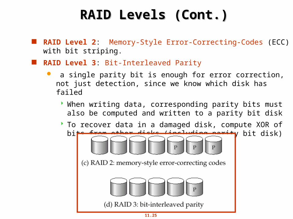
RAID Level 2: Memory-Style Error-Correcting-Codes (ECC) with bit striping.

RAID Level 3: Bit-Interleaved Parity

a single parity bit is enough for error correction, not just detection, since we know which disk has failed

When writing data, corresponding parity bits must also be computed and written to a parity bit disk

To recover data in a damaged disk, compute XOR of bits from other disks (including parity bit disk)

11.26


RAID Level 3 (Cont.) Faster data transfer than with a single disk, but fewer I/Os per

second since every disk has to participate in every I/O. Subsumes Level 2 (provides all its benefits, at lower cost).

RAID Level 4: Block-Interleaved Parity; uses block-level striping, and keeps a parity block on a separate disk for corresponding blocks from N other disks.

When writing data block, corresponding block of parity bits must also be computed and written to parity disk

To find value of a damaged block, compute XOR of bits from corresponding blocks (including parity block) from other disks.

11.27


RAID Level 4 (Cont.) Provides higher I/O rates for independent block reads than Level 3

block read goes to a single disk, so blocks stored on different disks can be read in parallel

Provides high transfer rates for reads of multiple blocks than no-striping

Before writing a block, parity data must be computed

Can be done by using old parity block, old value of current block and new value of current block (2 block reads + 2 block writes)

Or by recomputing the parity value using the new values of blocks corresponding to the parity block

– More efficient for writing large amounts of data sequentially

Parity block becomes a bottleneck for independent block writes since every block write also writes to parity disk

11.28


RAID Level 5: Block-Interleaved Distributed Parity; partitions data and parity among all N + 1 disks, rather than storing data in N disks and parity in 1 disk.

E.g., with 5 disks, parity block for nth set of blocks is stored on disk (n mod 5) + 1, with the data blocks stored on the other 4 disks.

11.29


RAID Level 5 (Cont.)

Higher I/O rates than Level 4.

Block writes occur in parallel if the blocks and their parity blocks are on different disks.

Subsumes Level 4: provides same benefits, but avoids bottleneck of parity disk.

RAID Level 6: P+Q Redundancy scheme; similar to Level 5, but stores extra redundant information to guard against multiple disk failures.

Better reliability than Level 5 at a higher cost; not used as widely.

11.30

Choice of RAID LevelChoice of RAID Level

Factors in choosing RAID level Monetary cost Performance: Number of I/O operations per second, and bandwidth

during normal operation Performance during failure Performance during rebuild of failed disk

Including time taken to rebuild failed disk RAID 0 is used only when data safety is not important

E.g. data can be recovered quickly from other sources Level 2 and 4 never used since they are subsumed by 3 and 5 Level 3 is not used since bit-striping forces single block reads to access

all disks, wasting disk arm movement, which block striping (level 5) avoids

Level 6 is rarely used since levels 1 and 5 offer adequate safety for almost all applications

So competition is between 1 and 5 only

11.31

Choice of RAID Level (Cont.)Choice of RAID Level (Cont.)

Level 1 provides much better write performance than level 5

Level 5 requires at least 2 block reads and 2 block writes to write a single block, whereas Level 1 only requires 2 block writes

Level 1 preferred for high update environments such as log disks

Level 1 had higher storage cost than level 5

disk drive capacities increasing rapidly (50%/year) whereas disk access times have decreased much less (x 3 in 10 years)

I/O requirements have increased greatly, e.g. for Web servers

When enough disks have been bought to satisfy required rate of I/O, they often have spare storage capacity

so there is often no extra monetary cost for Level 1!

Level 5 is preferred for applications with low update rate,and large amounts of data

Level 1 is preferred for all other applications

11.32

Hardware IssuesHardware Issues

Software RAID: RAID implementations done entirely in software, with no special hardware support

Hardware RAID: RAID implementations with special hardware

Use non-volatile RAM to record writes that are being executed

Beware: power failure during write can result in corrupted disk

E.g. failure after writing one block but before writing the second in a mirrored system

Such corrupted data must be detected when power is restored

– Recovery from corruption is similar to recovery from failed disk

– NV-RAM helps to efficiently detected potentially corrupted blocks

» Otherwise all blocks of disk must be read and compared with mirror/parity block

11.33

Hardware Issues (Cont.)Hardware Issues (Cont.)

Hot swapping: replacement of disk while system is running, without power down

Supported by some hardware RAID systems,

reduces time to recovery, and improves availability greatly

Many systems maintain spare disks which are kept online, and used as replacements for failed disks immediately on detection of failure

Reduces time to recovery greatly

Many hardware RAID systems ensure that a single point of failure will not stop the functioning of the system by using

Redundant power supplies with battery backup

Multiple controllers and multiple interconnections to guard against controller/interconnection failures

11.34

RAID Terminology in the IndustryRAID Terminology in the Industry

RAID terminology not very standard in the industry

E.g. Many vendors use

RAID 1: for mirroring without striping

RAID 10 or RAID 1+0: for mirroring with striping

“Hardware RAID” implementations often just offload RAID processing onto a separate subsystem, but don’t offer NVRAM.

Read the specs carefully!

Software RAID supported directly in most operating systems today

11.35

Optical DisksOptical Disks Compact disk-read only memory (CD-ROM)

Removable disks, 640 MB per disk

Seek time about 100 msec (optical read head is heavier and slower) Higher latency (3000 RPM) and lower data-transfer rates (3-6 MB/s)

compared to magnetic disks Digital Video Disk (DVD)

DVD-5 holds 4.7 GB , and DVD-9 holds 8.5 GB

DVD-10 and DVD-18 are double sided formats with capacities of 9.4 GB and 17 GB

Slow seek time, for same reasons as CD-ROM

Record once versions (CD-R and DVD-R) are popular data can only be written once, and cannot be erased. high capacity and long lifetime; used for archival storage

Multi-write versions (CD-RW, DVD-RW, DVD+RW and DVD-RAM) also available

11.36

Magnetic TapesMagnetic Tapes

Hold large volumes of data and provide high transfer rates Few GB for DAT (Digital Audio Tape) format, 10-40 GB with DLT

(Digital Linear Tape) format, 100 – 400 GB+ with Ultrium format, and 330 GB with Ampex helical scan format

Transfer rates from few to 10s of MB/s Currently the cheapest storage medium

Tapes are cheap, but cost of drives is very high Very slow access time in comparison to magnetic disks and optical disks

limited to sequential access. Some formats (Accelis) provide faster seek (10s of seconds) at cost

of lower capacity Used mainly for backup, for storage of infrequently used information,

and as an off-line medium for transferring information from one system to another.

Tape jukeboxes used for very large capacity storage (terabyte (1012 bytes) to petabye (1015 bytes)

11.37

Storage AccessStorage Access

A database file is partitioned into fixed-length storage units called blocks. Blocks are units of both storage allocation and data transfer.

Database system seeks to minimize the number of block transfers between the disk and memory. We can reduce the number of disk accesses by keeping as many blocks as possible in main memory.

Buffer – portion of main memory available to store copies of disk blocks.

Buffer manager – subsystem responsible for allocating buffer space in main memory.

11.38

Buffer ManagerBuffer Manager

Programs call on the buffer manager when they need a block from disk.

Buffer manager does the following:

If the block is already in the buffer, return the address of the block in main memory

1. If the block is not in the buffer

1. Allocate space in the buffer for the block

1. Replacing (throwing out) some other block, if required, to make space for the new block.

2. Replaced block written back to disk only if it was modified since the most recent time that it was written to/fetched from the disk.

2. Read the block from the disk to the buffer, and return the address of the block in main memory to requester.

11.39

Buffer-Replacement PoliciesBuffer-Replacement Policies

Most operating systems replace the block least recently used (LRU strategy)

Idea behind LRU – use past pattern of block references as a predictor of future references

Queries have well-defined access patterns (such as sequential scans), and a database system can use the information in a user’s query to predict future references

LRU can be a bad strategy for certain access patterns involving repeated scans of data

e.g. when computing the join of 2 relations r and s by a nested loops for each tuple tr of r do for each tuple ts of s do if the tuples tr and ts match …

Mixed strategy with hints on replacement strategy providedby the query optimizer is preferable

11.40

Buffer-Replacement Policies (Cont.)Buffer-Replacement Policies (Cont.)

Pinned block – memory block that is not allowed to be written back to disk.

Toss-immediate strategy – frees the space occupied by a block as soon as the final tuple of that block has been processed

Most recently used (MRU) strategy – system must pin the block currently being processed. After the final tuple of that block has been processed, the block is unpinned, and it becomes the most recently used block.

Buffer manager can use statistical information regarding the probability that a request will reference a particular relation

E.g., the data dictionary is frequently accessed. Heuristic: keep data-dictionary blocks in main memory buffer

Buffer managers also support forced output of blocks for the purpose of recovery (more in Chapter 17)

11.41

File OrganizationFile Organization

The database is stored as a collection of files. Each file is a sequence of records. A record is a sequence of fields.

One approach:

assume record size is fixed

each file has records of one particular type only

different files are used for different relations

This case is easiest to implement; will consider variable length records later.

11.42

Fixed-Length RecordsFixed-Length Records

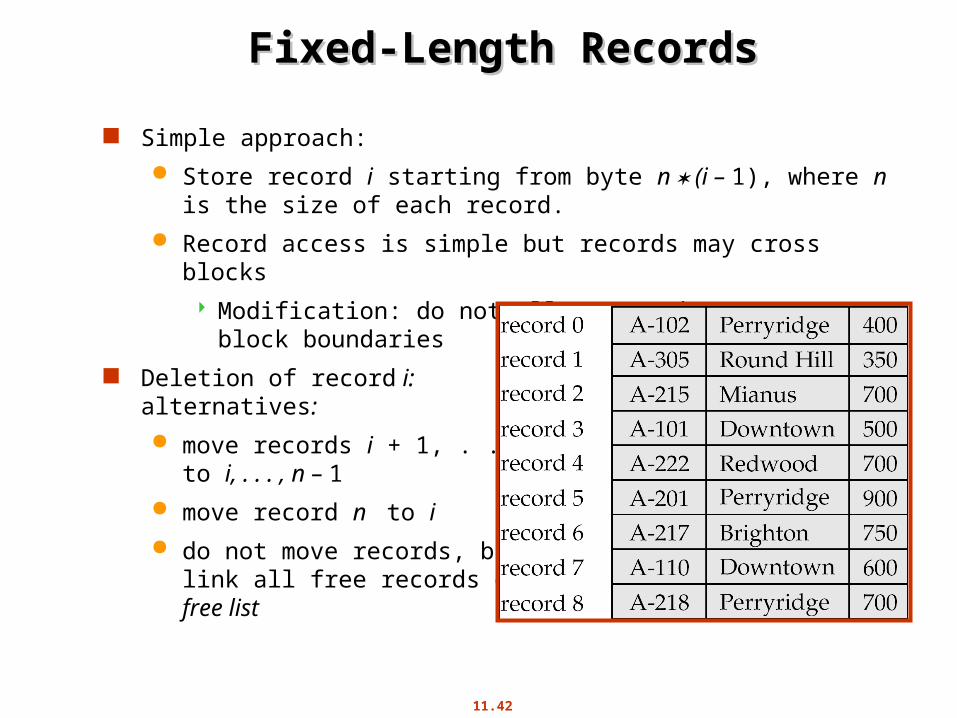
Simple approach:

Store record i starting from byte n (i – 1), where n is the size of each record.

Record access is simple but records may cross blocks

Modification: do not allow records to cross block boundaries

Deletion of record i: alternatives:

move records i + 1, . . ., n to i, . . . , n – 1

move record n to i

do not move records, but link all free records on afree list

11.43

Free ListsFree Lists

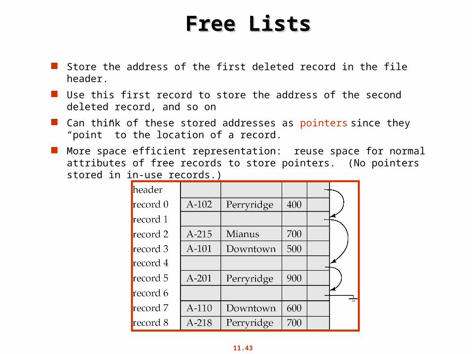
Store the address of the first deleted record in the file header.

Use this first record to store the address of the second deleted record, and so on

Can think of these stored addresses as pointers since they “point” to the location of a record.

More space efficient representation: reuse space for normal attributes of free records to store pointers. (No pointers stored in in-use records.)

11.44

Variable-Length RecordsVariable-Length Records

Variable-length records arise in database systems in several ways:

Storage of multiple record types in a file.

Record types that allow variable lengths for one or more fields.

Record types that allow repeating fields (used in some older data models).

11.45

Variable-Length Records: Slotted Page Variable-Length Records: Slotted Page StructureStructure

Slotted page header contains:

number of record entries

end of free space in the block

location and size of each record

Records can be moved around within a page to keep them contiguous with no empty space between them; entry in the header must be updated.

Pointers should not point directly to record — instead they should point to the entry for the record in header.

11.46

Organization of Records in FilesOrganization of Records in Files

Heap – a record can be placed anywhere in the file where there is space

Sequential – store records in sequential order, based on the value of the search key of each record

Hashing – a hash function computed on some attribute of each record; the result specifies in which block of the file the record should be placed

Records of each relation may be stored in a separate file. In a multitable clustering file organization records of several different relations can be stored in the same file

Motivation: store related records on the same block to minimize I/O

11.47

Sequential File OrganizationSequential File Organization

Suitable for applications that require sequential processing of the entire file

The records in the file are ordered by a search-key

11.48

Sequential File Organization (Cont.)Sequential File Organization (Cont.)

Deletion – use pointer chains

Insertion –locate the position where the record is to be inserted

if there is free space insert there

if no free space, insert the record in an overflow block

In either case, pointer chain must be updated

Need to reorganize the file from time to time to restore sequential order

11.49

Multitable Clustering File OrganizationMultitable Clustering File Organization

Store several relations in one file using a multitable clustering file organization

11.50

Multitable Clustering File Organization (cont.)Multitable Clustering File Organization (cont.)

Multitable clustering organization of customer and depositor:

good for queries involving depositor customer, and for queries involving one single customer and his accounts

bad for queries involving only customer results in variable size records Can add pointer chains to link records of a particular relation

11.51

Data Dictionary StorageData Dictionary Storage

Information about relations names of relations names and types of attributes of each relation names and definitions of views integrity constraints

User and accounting information, including passwords Statistical and descriptive data

number of tuples in each relation Physical file organization information

How relation is stored (sequential/hash/…) Physical location of relation

Information about indices (Chapter 12)

Data dictionary (also called system catalog) stores metadata: that is, data about data, such as

11.52

Data Dictionary Storage (Cont.)Data Dictionary Storage (Cont.)

Catalog structure

Relational representation on disk

specialized data structures designed for efficient access, in memory

A possible catalog representation:

Relation_metadata = (relation_name, number_of_attributes, storage_organization, location)Attribute_metadata = (attribute_name, relation_name, domain_type,

position, length)User_metadata = (user_name, encrypted_password, group)Index_metadata = (index_name, relation_name, index_type,

index_attributes)View_metadata = (view_name, definition)

Extra SlidesExtra Slides

11.54

Record RepresentationRecord Representation

Records with fixed length fields are easy to represent

Similar to records (structs) in programming languages

Extensions to represent null values

E.g. a bitmap indicating which attributes are null

Variable length fields can be represented by a pair (offset,length) where offset is the location within the record and length is field length.

All fields start at predefined location, but extra indirection required for variable length fields

Example record structure of account record

account_number

branch_name

balance

PerryridgeA-102 40010 000

null-bitmap

ExamplesExamples

11.56

File Containing File Containing account account Records Records

11.57

File of Figure 11.6, with Record 2 Deleted and File of Figure 11.6, with Record 2 Deleted and All Records MovedAll Records Moved

11.58

File of Figure 11.6, With Record 2 deleted and File of Figure 11.6, With Record 2 deleted and Final Record MovedFinal Record Moved

11.59

Byte-String Representation of Variable-Length Byte-String Representation of Variable-Length RecordsRecords

11.60

Clustering File StructureClustering File Structure

11.61

Clustering File Structure With Pointer ChainsClustering File Structure With Pointer Chains

11.62

The The depositordepositor Relation Relation

11.63

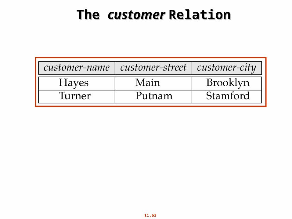
The The customer customer RelationRelation

11.64

Clustering File StructureClustering File Structure

11.65

11.66

Figure 11.4Figure 11.4

11.67


11.68


11.69


11.70

Byte-String Representation of Variable-Length RecordsByte-String Representation of Variable-Length Records

Byte string representationAttach an end-of-record () control character to the end of each recordDifficulty with deletionDifficulty with growth

11.71

Fixed-Length RepresentationFixed-Length Representation

Use one or more fixed length records:

reserved space

pointers

Reserved space – can use fixed-length records of a known maximum length; unused space in shorter records filled with a null or end-of-record symbol.

11.72

Pointer MethodPointer Method

Pointer method

A variable-length record is represented by a list of fixed-length records, chained together via pointers.

Can be used even if the maximum record length is not known

11.73

Pointer Method (Cont.)Pointer Method (Cont.)

Disadvantage to pointer structure; space is wasted in all records except the first in a a chain.

Solution is to allow two kinds of block in file:

Anchor block – contains the first records of chain

Overflow block – contains records other than those that are the first records of chairs.

11.74

Mapping of Objects to FilesMapping of Objects to Files

Mapping objects to files is similar to mapping tuples to files in a relational system; object data can be stored using file structures.

Objects in O-O databases may lack uniformity and may be very large; such objects have to managed differently from records in a relational system.

Set fields with a small number of elements may be implemented using data structures such as linked lists.

Set fields with a larger number of elements may be implemented as separate relations in the database.

Set fields can also be eliminated at the storage level by normalization.

Similar to conversion of multivalued attributes of E-R diagrams to relations

11.75

Mapping of Objects to Files (Cont.)Mapping of Objects to Files (Cont.)

Objects are identified by an object identifier (OID); the storage system needs a mechanism to locate an object given its OID (this action is called dereferencing).

logical identifiers do not directly specify an object’s physical location; must maintain an index that maps an OID to the object’s actual location.

physical identifiers encode the location of the object so the object can be found directly. Physical OIDs typically have the following parts:

1. a volume or file identifier

2. a page identifier within the volume or file

3. an offset within the page

11.76

Management of Persistent PointersManagement of Persistent Pointers

Physical OIDs may be a unique identifier. This identifier is stored in the object also and is used to detect references via dangling pointers.

11.77

Management of Persistent Pointers Management of Persistent Pointers (Cont.)(Cont.)

Implement persistent pointers using OIDs; persistent pointers are substantially longer than are in-memory pointers

Pointer swizzling cuts down on cost of locating persistent objects already in-memory.

Software swizzling (swizzling on pointer deference)

When a persistent pointer is first dereferenced, the pointer is swizzled (replaced by an in-memory pointer) after the object is located in memory.

Subsequent dereferences of of the same pointer become cheap.

The physical location of an object in memory must not change if swizzled pointers pont to it; the solution is to pin pages in memory

When an object is written back to disk, any swizzled pointers it contains need to be unswizzled.

11.78

Hardware SwizzlingHardware Swizzling

With hardware swizzling, persistent pointers in objects need the same amount of space as in-memory pointers — extra storage external to the object is used to store rest of pointer information.

Uses virtual memory translation mechanism to efficiently and transparently convert between persistent pointers and in-memory pointers.

All persistent pointers in a page are swizzled when the page is first read in.

thus programmers have to work with just one type of pointer, i.e., in-memory pointer.

some of the swizzled pointers may point to virtual memory addresses that are currently not allocated any real memory (and do not contain valid data)

11.79

Hardware SwizzlingHardware Swizzling

Persistent pointer is conceptually split into two parts: a page identifier, and an offset within the page.

The page identifier in a pointer is a short indirect pointer: Each page has a translation table that provides a mapping from the short page identifiers to full database page identifiers.

Translation table for a page is small (at most 1024 pointers in a 4096 byte page with 4 byte pointer)

Multiple pointers in page to the same page share same entry in the translation table.

11.80

Hardware Swizzling (Cont.)Hardware Swizzling (Cont.)

Page image before swizzling (page located on disk)

11.81


When system loads a page into memory the persistent pointers in the page are swizzled as described below

1. Persistent pointers in each object in the page are located using object type information

2. For each persistent pointer (pi, oi) find its full page ID Pi

1. If Pi does not already have a virtual memory page allocated to it,

allocate a virtual memory page to Pi and read-protect the page

Note: there need not be any physical space (whether in memory or on disk swap-space) allocated for the virtual memory page at this point. Space can be allocated later if (and when) Pi is accessed. In this case read-protection is not required.

Accessing a memory location in the page in the will result in a segmentation violation, which is handled as described later

2. Let vi be the virtual page allocated to Pi (either earlier or above)

3. Replace (pi, oi) by (vi, oi)

3. Replace each entry (pi, Pi) in the translation table, by (vi, Pi)

11.82


When an in-memory pointer is dereferenced, if the operating system detects the page it points to has not yet been allocated storage, or is read-protected, a segmentation violation occurs.

The mmap() call in Unix is used to specify a function to be invoked on segmentation violation

The function does the following when it is invoked

1. Allocate storage (swap-space) for the page containing the referenced address, if storage has not been allocated earlier. Turn off read-protection

2. Read in the page from disk

3. Perform pointer swizzling for each persistent pointer in the page, as described earlier

11.83


Page with short page identifier 2395 was allocated address 5001. Observe change in pointers and translation table.

Page with short page identifier 4867 has been allocated address 4867. No change in pointer and translation table.

Page image after swizzling

11.84


After swizzling, all short page identifiers point to virtual memory addresses allocated for the corresponding pages

functions accessing the objects are not even aware that it has persistent pointers, and do not need to be changed in any way!

can reuse existing code and libraries that use in-memory pointers

After this, the pointer dereference that triggered the swizzling can continue

Optimizations:

If all pages are allocated the same address as in the short page identifier, no changes required in the page!

No need for deswizzling — swizzled page can be saved as-is to disk

A set of pages (segment) can share one translation table. Pages can still be swizzled as and when fetched (old copy of translation table is needed).

A process should not access more pages than size of virtual memory — reuse of virtual memory addresses for other pages is expensive

11.85

Disk versus Memory Structure of ObjectsDisk versus Memory Structure of Objects

The format in which objects are stored in memory may be different from the formal in which they are stored on disk in the database. Reasons are:

software swizzling – structure of persistent and in-memory pointers are different

database accessible from different machines, with different data representations

Make the physical representation of objects in the database independent of the machine and the compiler.

Can transparently convert from disk representation to form required on the specific machine, language, and compiler, when the object (or page) is brought into memory.

11.86

Large ObjectsLarge Objects

Large objects : binary large objects (blobs) and character large objects (clobs)

Examples include:

text documents

graphical data such as images and computer aided designs audio and video data

Large objects may need to be stored in a contiguous sequence of bytes when brought into memory.

If an object is bigger than a page, contiguous pages of the buffer pool must be allocated to store it.

May be preferable to disallow direct access to data, and only allow access through a file-system-like API, to remove need for contiguous storage.

11.87

Modifying Large ObjectsModifying Large Objects

If the application requires insert/delete of bytes from specified regions of an object:

B+-tree file organization (described later in Chapter 12) can be modified to represent large objects

Each leaf page of the tree stores between half and 1 page worth of data from the object

Special-purpose application programs outside the database are used to manipulate large objects:

Text data treated as a byte string manipulated by editors and formatters.

Graphical data and audio/video data is typically created and displayed by separate application

checkout/checkin method for concurrency control and creation of versions

Documents

Storage and File Structure. 11.2 Chapter 11: Storage and File Structure Overview of Physical Storage Media Magnetic Disks RAID Tertiary Storage Storage