Embed Size (px)
Citation preview

Stock Trading Systems:
Analysis and Development of a System of Systems
An Interactive Qualifying Project
Submitted to the Faculty of
WORCESTER POLYTECHNIC INSTITUTE
In partial fulfillment of the requirements for the
Degree of Bachelor of Science
By
Joshua Levene
Justin Marcotte
Joshua Nottage
Date:
Report Submitted to:
Professors Michael Radzicki and Hossein Hakim of Worcester Polytechnic Institute
This report represents work of WPI undergraduate students submitted to the faculty as evidence of a
degree requirement. WPI routinely publishes these reports on its web site without editorial or peer
review. For more information about the projects program at WPI, see
http://www.wpi.edu/Academics/Projects.

2
Abstract
The goal of this project is to gain experience with trading the stock market by
experimenting with automated trading systems. The project consisted of three trading systems
that operated on different time frames and rules. After each system was established, it was
combined with the others into a system of systems to which simulated money was allocated
based on the quality of each individual system. This paper will describe and analyze each system
individually and as a system of systems.

3
Acknowledgements
We would first like to thank Professors Michael Radzicki and Hossein Hakim for their support,
guidance, and insight throughout the course of this Interactive Qualifying Project.
We would also like to thank Worcester Polytechnic Institute for allowing us the opportunity of
working on the project.
Finally, we would like to thank TradeStation for allowing us to utilize their services throughout
the development and completion of this project.

4
Table of Contents
Abstract ........................................................................................................................................... 2
Acknowledgements ......................................................................................................................... 3
Table of Contents ............................................................................................................................ 4
Table of Figures .............................................................................................................................. 6
Introduction ..................................................................................................................................... 8
Research and Background Information .......................................................................................... 9
An Introduction to Asset Classes ................................................................................................ 9
What are Equities? ................................................................................................................... 9
How are Currencies Traded? ................................................................................................... 9
Why This Project Traded Equities........................................................................................... 9
An Introduction to TradeStation ................................................................................................. 9
What is a Trading Platform? .................................................................................................... 9
What are Indicators?.................................................................................................................. 10
Strategies and their Components ............................................................................................... 10
Entry Rules ............................................................................................................................ 10
Exit Rules .............................................................................................................................. 11
Benefits and Disadvantages of Automatic and Manual Trading............................................... 11
Types of Trades ......................................................................................................................... 12
Types of Orders ......................................................................................................................... 12
What is meant by a System of Systems? ................................................................................... 13
Benefits of a System of Systems ........................................................................................... 13
Gap Terminology: What is a Gap? ............................................................................................ 13
Types of Gaps ........................................................................................................................ 14
Relative Strength Index (RSI) ................................................................................................... 15
Trend Following Terminology .................................................................................................. 16
Moving Average Crossovers ................................................................................................. 17
Bollinger Bands ..................................................................................................................... 18
Volatility Expansion Terminology: Average True Range ........................................................ 19
Description of the Systems ........................................................................................................... 19
Gap Strategy .............................................................................................................................. 19

5
Gap Up and Breakout ............................................................................................................ 20
Gap Up and Gap Fill .............................................................................................................. 21
Gap Down and Breakout ....................................................................................................... 21
Gap Down and Gap Fill ......................................................................................................... 21
Trend Following Strategy.......................................................................................................... 22
Volatility Expansion Strategy ................................................................................................... 23
Analysis of the Systems ................................................................................................................ 25
Development and Analysis of the Gap Strategy ....................................................................... 25
Choosing a Stock ................................................................................................................... 25
Choosing an Indicator ............................................................................................................ 27
Back-Testing, Walk-Forward, and Analysis of the Gap Strategy ......................................... 28
Evaluating the System using Expectancy, Expectunity, and System Quality ....................... 31
Monte Carlo Simulation and Position Sizing ........................................................................ 32
Development and Analysis of the Trend Following Strategy ................................................... 36
Development and Analysis of the Volatility Expansion Strategy ............................................. 38
Technical Analysis of the System ......................................................................................... 39
How the system performs with BEAM ................................................................................. 40
How the system performs with V .......................................................................................... 45
How the system performs with ADBE .................................................................................. 49
System Comparison and System of Systems Analysis ............................................................. 53
Conclusions and Looking Forward ............................................................................................... 54
Works Cited .................................................................................................................................. 57
Appendices .................................................................................................................................... 60
Gap Strategy Code .................................................................................................................... 60
Gap Up ................................................................................................................................... 60
Gap Down .............................................................................................................................. 61
Trend Following Strategy Code ................................................................................................ 62
Facebook Strategy ................................................................................................................. 62
Google Strategy ..................................................................................................................... 63
Volatility Expansion Strategy Code .......................................................................................... 64

6
Table of Figures
Figure 1: TradeStation Account Growth......................................................................................... 8
Figure 2: Gap Illustration ...............................................................................................................14
Figure 3: Moving Average Crossover Illustration ........................................................................18
Figure 4: Bollinger Bands Illustration ..........................................................................................18
Figure 5: Volatility Expansion Strategy .......................................................................................24
Figure 6: Gap Up History Summary ............................................................................................. 26
Figure 7: BP Back-Testing Performance Summary ......................................................................29
Figure 8: BP Equity Curve ............................................................................................................29
Figure 9: Gap Optimized Parameters ............................................................................................30
Figure 10: Walk-Forward Results ..................................................................................................31
Figure 10a: Gap Up Longs .............................................................................................31
Figure 10b: Gap Up Shorts .............................................................................................31
Figure 10c: Gap Down Longs .........................................................................................31
Figure 10d: Gap Down Shorts ........................................................................................31
Figure 11: Gap Strategy Analysis Results ....................................................................................32
Figure 12: BP Monte Carlo Simulation ........................................................................................34
Figure 12a: BP Monte Carlo Simulation and 95% Confidence Interval ........................34
Figure 12b: BP Monte Carlo 95% Confidence Interval Prediction ................................ 34
Figure 12c: BP Equity Curve Before Fixed Fractional Position Sizing .........................35
Figure 12d: BP Equity Curve After Fixed Fractional Position Sizing ............................35
Figure 13: Facebook Back-Testing Performance Summary .........................................................36
Figure 14: Google Back-Testing Performance Summary .............................................................37
Figure 15: BEAM Analysis .......................................................................................................... 40
Figure 15a: BEAM Optimized Parameters .....................................................................40
Figure 15b: BEAM Back-Testing Performance Summary ............................................41
7
Figure 15c: BEAM Efficiency .........................................................................................42
Figure 15d: BEAM Equity Curve ....................................................................................42
Figure 15e: BEAM Walk-Forward Cluster Analysis .......................................................43
Figure 15f: BEAM Walk-Forward Results ......................................................................44
Figure 15g: BEAM System Quality .................................................................................44
Figure 16: V Analysis ...................................................................................................................45
Figure 16a: V Optimized Parameters ...............................................................................45
Figure 16b: V Back-Testing Performance Summary .......................................................46
Figure 16c: V Efficiency ..................................................................................................46
Figure 16d: V Equity Curve .............................................................................................47
Figure 16e: V Walk-Forward Cluster Analysis ...............................................................47
Figure 16f: V Walk-Forward Results ..............................................................................48
Figure 16g: V System Quality .........................................................................................48
Figure 17: ADBE Analysis ...........................................................................................................49
Figure 17a: ADBE Optimized Parameters .......................................................................49
Figure 17b: ADBE Back-Testing Performance Summary ...............................................49
Figure 17c: ADBE Efficiency ..........................................................................................50
Figure 17d: ADBE Equity Curve .....................................................................................51
Figure 17e: ADBE Walk-Forward Cluster Analysis .......................................................51
Figure 16f: ADBE Walk-Forward Results ......................................................................52
Figure 17g: BEAM System Quality .................................................................................52
Figure 18: System Quality Comparison ........................................................................................54

8
Introduction
In today’s economy, many people consider financial security to be of a paramount
importance. Electronic trading platforms provide individuals with opportunities to trade in the
stock market, which they would otherwise not have. Due to this, many people engage in trading
without the proper background and knowledge. This exposes them to a great deal of risk as they
try to enter the world of professional trading. Instead of securing their financial future, many
people are putting their savings at risk.
Financial security has been a growing concern since the worldwide recession in 2008.
People have started taking it upon themselves to control their personal finances, rather than
relying on other institutions. For instance, 401K accounts have grown in popularity over the
years. Not only are 401K accounts cheaper for employers to provide, but the employee decides
where their money is invested. They provide employees more control over their personal
finances (Wall Street Journal, 17 April 2014). Furthermore, personal savings are an important
part of preparing for retirement. But, reinvesting money is more practical and proactive than
leaving it in a bank. This, along with the availability of electronic trading, has led to the growth
in the popularity of trading. Without employing a proper trading strategy, however, the stock
market can be a dangerous place for everyday people to allocate their money.
Figure 1: TradeStation Account Growth (Forex Magnates, 1 May 2014)
The primary purpose of this Interactive Qualifying Project is to create a trading system
that would be able to generate a profit from the stock market. This was accomplished by
experimenting with trading systems over time and studying patterns in the stock market in order
to exploit them. In order to increase the chances of making a profit, each student developed a
trading system individually. Each individual system was then combined into a robust system of
systems.

9
Research and Background Information
An Introduction to Asset Classes
What are Equities?
Equities, or stocks, represent ownership in a company. They are also one of the main
ways for companies to raise capital. In the United States, the two main equity markets are the
New York Stock Exchange and the NASDAQ. In the United States, equity markets open at 9:30
AM and close at 4PM Eastern Time.
How are Currencies Traded?
Currencies are traded in pairs on the currency market. Unlike equities, currencies can be
traded almost any time at all during the week, but the currency market does close each weekend.
Additionally, currencies are not traded on a central exchange like stocks. In other words,
currency trading does not have any exchange comparable to the New York Stock Exchange or
the NASDAQ (Schlossberg). Another unique aspect of currency trading is that it can be highly
leveraged. The amount of leverage depends on the broker, but currency trades could be as highly
leveraged as fifty to one. If a trader’s leverage was fifty to one, for an account of $1000, they
could trade up to $50000 worth of currency.
Why This Project Traded Equities
This project traded equities because trading shares of stock was more comfortable than
trading currency pairs. Another benefit to trading stocks is that the stock markets close every
night, which relieves traders of the obligation to stay up at night watching their trades.
Additionally, the fact that the stock market closes every night allows the use of different trading
strategies, such as gap strategies, to trade stocks.
An Introduction to TradeStation
What is a Trading Platform?
A trading platform is software that anyone can use to buy and sell different financial
assets. Trading platforms are run by brokers who buy and sell assets for customers. For this
project, TradeStation was the trading platform of choice. There is usually a fee attached to
having an account with a trading platform and there are also commission charges for each trade
that is made. Trading platforms have helped change the trading world because now nearly
anyone can be an active participant in the market. Trading platforms also are equipped with a

10
variety of tools that allow traders to take analytical approaches to their trades. Since this project
involved using Tradestation, an explanation of some of the tools that are provided by
TradeStation has been included.
What are Indicators? An indicator is one type of tool provided by Tradestation. An indicator is a statistical
measure that allows for the analysis of economic trends (TradeStation). As a trader, one looks at
different indicators to try to predict the future behavior of a stock or the market as a whole. If a
trader discovers that a stock moves in a predictable manner relative to what an indicator is
showing, they can exploit that behavior by buying or selling that stock when the indicator
exhibits that behavior. Then, the trader can take a position in the market before the price begins
to move in the direction that the indicator predicted. TradeStation provides several pre-
programmed indicators on its platform, but traders can also create their own indicators.
Strategies and their Components
A trading strategy is a set of rules for buying and selling financial assets. These rules are
usually based on information provided by one or more indicators. TradeStation provides its own
pre-programmed strategies, but its platform also allows traders to create their own strategies.
Strategies are a crucial part of successful trading because they are composed of a well-defined
set of rules that predict future market behaviors based on historical data. Without this knowledge
it is impossible to predict the movement of the market. There are several different components
in one trading strategy. For instance, in order to have a complete trading strategy, one must have
entry rules, exit rules, position sizing rules, and sometimes timeframe rules.
Entry Rules
Entry rules are the part of a strategy that puts you into the market. If the entry rule
conditions are met, then a buy or sell short order is placed. There are three different types of
entry rules. The first are set-up rules. These are rules that prepare a trader for an upcoming
trade. For instance, in a gap strategy, a set-up rule may be “If the open of the day is higher than
the high of yesterday”. If this condition is met, the trader knows that a trade may be coming up
in the near future. The next type of entry rule is a trigger rule. This is the rule that actually
produces an order and it should be designed to get a trader into the market at the optimal time.
An example of a trigger rule is “If the long-term moving average crosses over the short-term

11
moving average, then buy 100 shares”. The last type of entry rule is called a filter. This is a rule
that prevents a trade from being executed for some specific criteria. A simple filter rule is “If
there have been no trades today”. This filter rule prevents more than one trade being executed in
a day. Entry rules can be a difficult thing to balance. On the one hand, a trader wants enough
rules to keep them out of bad trades, but on the other hand, a trader cannot have so many rules
that they only make a few trades a year.
Exit Rules
Exit rules are rules that remove a trader from the market. Ideally, exit rules end a trade
while a trader is making a profit. Exit rules are also an important part of controlling losses.
Some examples of exit strategies are exiting after a set number of bars, exiting after a long and a
short moving average have crossed over again and exiting after a gap has been filled. Of course,
different exit rules work well with different strategies and it is a matter of testing and
experimentation to find rules that work with a particular trading system. Another important part
of exit rules are stop losses and profit margins. These are more specific types of exit rules. Stop
losses protect traders from large losses by removing them from the market if they lose a specific
dollar amount on a trade or if they lose a certain percent of capital on a given trade. A stop loss
is set at the largest amount that a trader is willing to lose in one trade. A profit margin is based
on a similar idea. A profit margin is set at a dollar amount, or a percentage of capital that a
trader would be satisfied with winning in one trade. By using a profit margin, a trader is saying
that the potential benefits of staying in an already good trade do not outweigh the risks of staying
in that trade. Clearly, stop losses and profit margins are important tools in managing trading
risk.
Benefits and Disadvantages of Automatic and Manual Trading
Manual trading is a process in which a trader analyzes markets and assets and decides for
themselves which trades to take. This is the more traditional form of trading. On the other hand,
automatic trading relies on programming strategies that will alert traders when an available trade
meets their criteria. This is not to say that manual trading is not scientific compared to automatic
trading. In fact, traders that use both methods still need to develop rules for themselves that they
believe will lead to profitable trades when followed. Though there has been a recent shift in
popularity from manual to automatic trading, many traders still employ elements of manual
trading. Essentially, they are trading a mix of both types of trading (Kennedy, 9 April 2014). As

12
one might imagine, there are benefits to both trading techniques. The benefits of automatic
trading are that a computer always follows the trading rules perfectly, it will not make order
mistakes, it can handle more information than a human, a computer will not miss a buy signal
and computers do not get tired. On the other hand, there are also advantages to manually trading.
For instance, humans can take into consideration the whole global economy when making a
trade. Also, humans can sense when a trade is not going well or when a trade is not moving
quickly enough and can reason to close the trade (Tucci, 7 April 2014). Traders that combine
these two styles of trading are trying to get the best of both worlds by combining the precision of
an automated trading system with the logic of human reasoning. For instance, a trader may set
up an automatic trading system, but may chose to reject some trades that the system suggests
based on the overall state of the economy, which is a factor that an automatic trading system
cannot take into account. For this project, automatic trading systems have been used because of
the accuracy and ease of executing trades.
Types of Trades In stock trading, a long trade is when a trader buys shares anticipating that the value of a
stock will increase. When the trader wants to get out of the trade, he/she will sell the shares that
he/she bought and will earn a profit or loss based on the spread of the buy and sell prices.
A short trade in stock trading is slightly more complicated than a long trade. By shorting
a stock, traders mean that they are initiating a trade by selling a stock. In order to sell a stock
that they do not initially possess, a trader must borrow that stock from someone, usually a
broker. After they sell the stock, they buy it back at ideally a lower price than they sold it. Then,
they give the borrowed stock back to the broker. This is one way that a trader can take
advantage of a decrease in price.
Types of Orders A market order is placed when a trader wants an order filled as soon as possible. The
trader will get their order filled, but not necessarily at the price that is best for them. Instead,
they settle for buying or selling at market value. In contrast, a limit order is set at a specific price
or better. Thus, a trader is not guaranteed that their order will be filled. There are clearly
advantages to either type of order and traders sometimes just choose an order type based on their
preference. Another type of order is a stop order. Stop orders are orders that trigger market or

13
limit orders once a specific price level is reached. Stop orders can be used as a tool to confirm
the direction of the market before entering a trade.
What is meant by a System of Systems? For this project, the final trading system was a combination of three different trading
systems. Each member of the project group designed and tuned one trading system with input
and advice from other members. The three systems that have been developed are a gap strategy,
a trend following strategy and a volatility expansion strategy.
Benefits of a System of Systems
Trading experts agree that there is no “Holy Grail” trading system. No system works all
the time and trading the stock market is never easy (Mitchell, 8 April 2014). But, one’s odds of
making money in the stock market can be improved by using multiple systems. For instance, a
longer term system that is resistant to market noise can work well with a shorter term system to
create a more consistent and robust system of systems (Wyckoff, 6 April 2014). The major
attraction of using a system of systems in trading is that it provides diversification. The three
systems in this project trade using different indicators, different frequencies, and different
timeframes. This type of diversification is desirable because when one strategy is performing
poorly, the other systems are not exposed to the same types of risk and variance as the poorly
performing strategy and should continue to perform well. This will result in more even growth
over time and will help prevent large consecutive losses.
Gap Terminology: What is a Gap? In trading, a gap occurs when the open of one bar is at a different price level than the
close of the previous bar (Seven Trading Systems, 10 January 2014). Usually, gaps are looked at
on a daily scale. This means that traders say a gap occurs when the open of the day is at a
different price than the close of yesterday. Naturally, there are two basic forms of gaps: gaps up
and gaps down. Most traders consider a gap up as the open of the day being higher than the
close of yesterday and a gap down as the open of the day being lower than the close of yesterday.
However, for the gap trading system in this project, a gap up is recognized only if the open of the
day is higher than the high of yesterday and a gap down is recognized only if the open of the day
is lower than the low of yesterday.

14
Figure 2: Gap Illustration (StockCharts, 6 April 2014)
It is also important to consider what causes these gaps. Gaps occur because traders place
buy and sell orders before the market opens, causing the opening price for the day to be different
than the close of the previous day. But, why are so many orders being placed before the market
opens? One reason is that news about a company may have been released after the close of the
market on the previous day (StockCharts 6 April 2014). So, the opening stock price is trying to
correct itself to reflect that news. These gaps can be analyzed and used as the basis for many
different trading strategies.
Another important note is that when traders talk about gaps, they are usually referring to
gaps in stock prices as opposed to currency pairs. This is simply because the stock market closes
every day, which means that each morning a stock may have gapped. The currency market,
however, only closes once a week. So, there can be at most one gap a week in a currency.
Simply put, there are more opportunities to trade gaps with stocks than with currency pairs, so
stocks are generally traded with gap strategies.
Types of Gaps
Once a stock has gapped, there are several patterns and behaviors that traders look for in
the stock price. These behaviors usually become the basis for a trading system. In this project,
two different behaviors have been explored: filling the gap and breakouts.

15
Filling the Gap
The term filling the gap usually refers to the situation in which the price of a stock that
has gaped returns to the price at the close of the day before. For example, if BP had closed at
47.50 yesterday and then gapped up to 48.00 today, BP is said to have filled the gap if its price
reaches 47.50 again today. So, if you were a trader and you expected BP to fill the gap, you
would short BP at the open and then buy to cover once BP had filled the gap. This is just one
example of how this pattern can be incorporated into a trading system.
Breakouts
A stock that has a breakout behaves the opposite of a stock that fills the gap. If a stock
gaps up, then there is a breakout if the price of the stock continues to increase. If a stock gaps
down, then there is a breakout if the price of the stock continues to decrease. For example, if BP
closed at 47.50 yesterday and then gapped up to 48.00 today and we expected a breakout, we
would buy BP at 48.00 a share at the open because we would expect the price to keep increasing.
Breakouts and filling the gap are two behaviors that will be traded by the gap trading system
portion of our project.
Relative Strength Index (RSI) The Relative Strength Index was created by J. Welles Wilder in 1978 (Thygesen, 4 April
2014). The RSI is a well known and widely used indicator. This indicator measures momentum
by comparing the extent of a stock’s recent gains and losses by transforming this info into a
number between 0 and 100 (Thygesen, 4 April 2014). There are two numbers which are
important when using the RSI as an indicator. The first is the overbought level and the second is
the oversold level. These levels can be used as signals to buy or sell a stock. For instance, if a
stock has an RSI above the overbought level that means that there is recent momentum in the
stock. But, once the RSI falls back below the overbought level, this can be taken as a sell signal
because it indicates that the stock has recently lost momentum. When he created the RSI, Welles
Wilder suggested that traders use a value of 70 to indicate that a stock is overbought and a value
of 30 to indicate that a stock is oversold (Nathan, 9 April 2014). But, many traders deviate from
this suggestion and use more restrictive overbought and oversold levels. This makes their trades
more selective and more likely to be profitable. Another part of the RSI that traders can
manipulate is the number of bars that the indicator looks at. Welles Wilder suggested that the
indicator use a length of 14, but different traders may use different lengths based on their trading

16
system (StockCharts, 7 April 2014). For example, a scalping system would want to use a shorter
length, since they are looking for many small, quick trades.
Trend Following Terminology Trend Analysis is a common method used by most traders and investors. This method of
trading attempts to predict trends or patterns in the market by analyzing data from the past.
Based on this analysis, traders that use a trend following strategy will make predictions on future
market trends. Aside from analyzing past market trends, a trend following strategy will always
ride a trend until a sudden change is detected. An example of this would be, taking a long
position in a bull market and then exiting that position if the strategy indicates that the market is
experiencing a pullback. The terms, “bull” and “bear”, are used to describe market trends. A bull
market identifies a market with an upward trend while a bear market identifies one with a
downward trend (Cruset, 2005, Page 5).
Trend following strategies are popular for several reasons and are especially common
among large hedge funds due to their capacity to support large amounts of equity. Given a basic
understanding of trend following systems, it is likely that a trader will make a profit with the
right strategy. Typically, trend following system rules are simple and can detect major trends by
measuring the price variation from certain reference values. When a trend is detected, a position
is established in favor of the trend. Other major advantages to trend following systems are that
profitable trades are not exited until the trend changes and unprofitable trades can be detected
and avoided with a predefined stop loss point. This means that once a profitable position is
established, the system will hold that position, yielding consistent profits until a change is
detected. Rather than trading manually, where a trader will typically hold an unprofitable
position in hopes that the market will turn, automated trading systems allows the trader to set a
stop loss point where, if a certain quantity of money is lost, the system will exit the position and
greater losses are avoided (Cruset, 2005, Page 5).
Unfortunately, the trader does take on a certain amount of risk when using trend
following systems, as a trader typically would when using any trading strategy. In the case of
trend following systems, traders do need to take into account how much risk they are willing to
take. Traders must determine a maximum amount of money they would be willing to lose in a

17
single position. It is always possible that market expectations can be wrong, which is a factor that
many inexperienced traders do not take into account when trading.
There are several concepts that can be used to detect a trend. For this project, the trend
following system experimented with Moving Average Crossovers and Bollinger Bands. These
concepts will be explained later on. Although other trend detecting techniques exist, they are
usually based on more complex indicators and require additional information in order to satisfy
their rules. The complexity of the techniques, however, does not affect how profitable a system
can be. Moving Average Crossovers and Bollinger Bands both use data provided by an average
market day. These values are the Open, High, Low, and Close. The open and close are the prices
at which a stock began and ended the day. The high refers to the highest price the stock reached
during the day and the low refers to the lowest price. Neither technique takes into account
volume or other intraday information.
Normally, trend following strategies will only take a few trades over the course of a year.
This happens because most strategies are designed to take advantage of big market swings but
this involves holding a position for a large amount of time which may lead to major losses due to
noise in the market. Noise occurs when price and volume fluctuations in the market cause
confusion regarding a trader’s interpretation of market direction. The shorter the time frame, the
more difficult it is to separate noise from meaningful market movements which can lead to major
losses when holding a position that attempts to follow a trend over an extended period of time.
Moving Average Crossovers
A moving average or “MA” is a type of indicator, widely used in technical analysis. It
helps smooth out price action by filtering out market noise from random price fluctuations.
Moving averages are also trend-following indicators as they are based on past prices and they are
used to identify trend direction. Moving average crossovers are a type of moving average.
Crossovers occur when a faster moving average (a moving average that covers a shorter period
of time) crosses either above or below a slower moving average which, covers a longer period of
time. When the faster moving average crosses above the slower moving average, it is considered
a bullish crossover and when the faster moving average crosses beneath the slower moving
average, it is a bearish crossover. When the longer moving average is in an uptrend, it indicates
that the market is strong. A buy signal is then established when the faster moving average

18
crosses above the slower moving average. A sell signal is also established when the faster
moving average crosses below the slower moving average. Using these strategies, as stated
before, involves spending a lot of time in the market. (“Moving Average Crossovers”)
Figure 3 below shows how one would trade using a moving average crossover.
Figure 3: Moving Average Crossover Illustration (Mulloy, 22 April 2014)
Bollinger Bands
Bollinger Bands, like moving averages, are a type of indicator created by John Bollinger.
Bollinger Bands were created to provide a relative definition of the high and low and consist of
three bands. The upper band indicates high prices, a middle band, and the lower band, which
indicates low prices. The middle band is usually a type of moving average that acts as a base for
the upper and lower bands. This indicator allows traders to recognize patterns in the market and
is useful when comparing price activity to the action of indicators. The space above and below
the middle band is determined by volatility and the volatility is normally the standard deviation
of the data that is used to determine the average. Traders will use the upper and lower bands as
indicators to buy and sell depending on whether a stock goes above the upper band or below the
lower band. An advantage to this indicator is that the parameters and the number of standard
deviations can be adjusted to work best for the trader (Bollinger, 26 April 2014).
Figure 4: Bollinger Bands Illustration (Bollinger, 26 April 2014)

19
Volatility Expansion Terminology: Average True Range Volatility expansion systems, also known as volatility breakout systems, tread a path
somewhat between how gap strategies and trend strategies operate. When volatility becomes
high enough (due to a “volatility expansion”) and the price of a stock moves significantly outside
of its normal range and noise (in a move called a “breakout”), the theory behind the system states
that it will continue to move in that direction for about one to three days, usually two days. While
there are many ways to measure volatility in the market, including but not limited to the VIX
factor, standard deviation, variance and average true range, the only one covered in the written
strategy is the average true range. An important part of the average true range naturally is the
true range, which is the difference between two other variables: the true high and the true low.
The true high is calculated as the higher of either today’s high or previous close. The true low,
analogously calculated, is calculated as the lower of today’s low or previous close. This range
helps determine a realistic range for trades on the day (Tradestation, 9 April 2014). The average
true range is simply the average of the true ranges of a user-defined number of previous bar.
(Tradestation, 9 April 2014).
Description of the Systems As mentioned previously, each member of the group worked on their own individual
trading system with the intention of combining systems to make a more comprehensive system
of systems at the end of the project. Joshua Nottage developed a system based on a gap strategy,
Joshua Levene developed a trend following system, and Justin Marcotte developed a volatility
expansion system.
Gap Strategy In a traditional gap strategy, the main focus is finding prices at the open of the market
that differ from closing prices from the day before and exploiting their differences to make
profit. This system is unique in that it does not look at closing prices from the day before, but
instead looks at the highs and lows of yesterday. This system attempted to trade four different
scenarios. The four scenarios are a gap up and a breakout, a gap up and a gap fill, a gap down
and a breakout and a gap down and a gap fill. These different scenarios have slightly different
trading rules associated with them, but are mostly closely related.

20
The main indicator used in this strategy is the Relative Strength Index, or RSI. This
measures if a financial asset is currently overbought or oversold. The logic behind the strategy is
that if a stock gapped, then it probably will be overbought or oversold at least for a brief period
of time at the open. In that case, a buy or sell signal can be determined based on how quickly the
RSI moves after the open. The other unique characteristic of this strategy is the definition of a
gap. Traditionally, a gap up occurs if the open of the day is higher than the close of yesterday.
However, in this strategy, a gap up only occurs if the open of the day is higher than the high of
yesterday. This limits the amount of small gaps that are traded on the strategy and thus lowers
the potential for stagnant trades. Also, since there is a maximum of one gap on a stock in a given
day, this strategy limits the trades that can be made to one trade a day. Lastly, this strategy is
traded on five minute bars because they worked well with the system. Five minute bars are short
enough to show trends for a day trader, but not so short that they consist primarily of noise.
Gap Up and Breakout
For a gap up, it is expected that the RSI will be above the overbought level at the open. If
there is a gap up and a breakout is expected, this means that a long position will be taken.
Whether a breakout is expected or not depends on the behavior of the RSI. In order to generate a
buy signal, the RSI must continue to be overbought for a good amount of time. This shows that
there is momentum behind the gap up that occurred at the open. The amount of time that the RSI
needs to be above the overbought level can be optimized, but a general rule is that one wants the
RSI to stay above the overbought level until after 10:00AM. It is the theory of some traders that
the high and lows of the day are set between the open at 9:30 and 10:00. If the RSI stays
overbought after this time, it is expected that the price of the stock that gapped will break
through the resistance levels created between 9:30 and 10:00. Once again, the optimal time to
wait could be more than 10:00 and this optimal time can be continually changed as the system is
being traded. The last condition that needs to be met is the filter condition. For this system to
take a long on a gap up, the market must be moving in the right direction. This is mostly a safety
net to make sure that unwise trades are not executed. This system simply requires that the
current high is above the high of yesterday, which again guarantees that there is momentum in
the trades that are taken.

21
Gap Up and Gap Fill
Once again, for a gap up, the RSI is expected to begin the day above the overbought
level. If a stock is expected to fill the gap, the stock should be short sold and then bought back
when the price has fallen. Whether a gap fill is expected depends on the movement of the RSI.
So, if the RSI crosses under the overbought level before an optimized time (for example
10:00AM), the stock would be sold short because the stock is losing momentum and the price
should go down. As before, the system included one more condition as a safety net to ensure
that bad trades are not executed. This condition is that the current price must be above the high
of yesterday, but below the open of today. Otherwise, a trade cannot be executed. This filter
condition ensures that the stock price is moving in the correct direction, but also that the gap has
not been filled yet, since the current price must be above the high of yesterday. If the gap has
been filled already, then it is too late to make a trade and the system will stay out of the market.
Gap Down and Breakout
In a gap down and breakout, the price of a stock is expected to continue to decline after a
gap down occurs. In this system, the RSI will help determine if a gap down is likely to breakout.
In order to produce a sell short signal, the RSI needs to remain below the oversold level until a
specific time of day, which can be optimized by back testing. Another condition is that the price
at which a trade is taken is lower than the open of the day. This filter rule ensures that the price
of the stock is moving in the correct direction. If these conditions are met, the strategy creates a
sell short signal and the price of the stock should continue to decrease.
Gap Down and Gap Fill
In a gap down and gap fill, the price of a stock is expected to increase back to the low of
yesterday. Sometimes, the price will rise even above the low of yesterday, creating room for
more profits. In order for a buy signal to be generated on a gap down, the RSI must start the day
below the oversold level and cross over the oversold level early in the day. The crossover needs
to be early in the day because there needs to be time available for the stock price to change
throughout the day, since this is a day trading system. Additionally, if the system only looks for
crossovers early in the day, it will not interfere with the gap down and breakout rules described
above. The filter rule is that the price of the stock in moving in the right direction. In order to
buy shares, the current price needs to be above the open, but below the low of yesterday because
the gap cannot be already filled when the purchase is made.

22
Trend Following Strategy As previously mentioned, trend following strategies are designed to follow trends, detect
big swings in the market, and will typically make very few, large trades over the course of a
year. Given these factors, trend following strategies are very susceptible to noise, which can lead
to large market losses. The trend following strategy developed for this project, attempts to avoid
noise and take a larger amount of trades over the course of a year but before the strategy could be
implemented, stocks needed to be chosen.
Research was conducted on stocks that were known to trend and were evaluated based on
popularity and the company’s activity and future plans. Of the stocks that were researched,
Facebook (FB) and Google (GOOG) stood out. Both stocks were very popular and had been in
an upward trend, or bull trend, for a few weeks. Facebook, Inc. had plans to incorporate many
other social media applications such as WhatsApp and Instagram. Many other companies were
looking towards Facebook for advertising purposes. Companies pay Facebook consistently in
order to allow them to advertise on Facebook’s page and phone application. Google’s future
plans seemed even more promising as they had an entire line of different products coming out
between 2013 and 2015 such as Google Play and Google Glass. Google also made several
hardware sales to Lenovo and other companies that were seeking to expand. The third stock that
was chosen was Randgold Resources Limited (GOLD). This was chosen as an experimental
stock used to test certain strategies and fiddle with the EasyLanguage code.
The trend following strategies that were developed to trade Google and Facebook were
very similar in order to maintain a certain degree of consistency when testing. Both strategies
used intra-day intervals and were tested for a year of trading. The last date was set to March 26,
2014 and they were tested over the course of one year previous to this date. On March 27,
Google split its stock. The stock was split 2-for-1. This means that, the company’s board of
directors decided to increase the number of shares outstanding by issuing more shares to current
shareholders. The 2-for-1 split means that for every share that a shareholder has, they were
issued one more additional share. Basically, the number of shares doubled and the value of each
share was cut in half. Now, there are two separate symbols that can be traded for the same
company. In the case of Google (GOOG) there is a GOOG and a GOOGL symbol and one is
favored over the other.

23
In the case of Google, the strategy that was used traded over 120-minute bars, which
proved to be the most profitable way to trade this stock. The same strategy was used for
Facebook and Randgold. Facebook was traded over 60 to 90-minute bars and 45-minute bars
were used for Randgold. These strategies will be explained in more detail in the Data Analysis
section for the Trend Following Strategy.
Volatility Expansion Strategy The volatility expansion strategy shown for this project makes use of a great number of
inputs, which in turn determine values for variables of the strategy. First of which is the low
volume breakout fraction for longs, marked simply as FrLv0. Similarly, for high volume, is the
high volume breakout fraction for longs, similarly marked as FrLv1. The next of which is
referred to as MMFrL, a volatility multiplier for money management on longs. Next, V0 and V1
are low and high volatility measurements, respectively. Finally, AvData is how many previous
bars of data are used for the average true range. While some of these were “variables” in the
original code, they were moved to the input section based on that they were constant. While
having so many variables makes optimization difficult, it also allows for greater customization.
The inputs are channeled into variables. ATR, the average true range, takes into account
the true range over AvData amounts of data. ML and BL create a breakout line for longs, with
slope ML and intercept BL. The slope ML is calculated by dividing the difference between
FrLv1 and FrLv0 by the difference between V1 and V0. The intercept BL is calculated by
subtracting FrLv0 by the product of ML and V0. The entry fraction for longs, FrL, is determined
by multiplying the slope of the breakout fraction line by ATR and adding the intercept.
Note that the ML and BL are essentially constant, due to all of their components being
constant. However, ATR can change every bar, and as such, so may FrL. These two variables
determine the long and one of the two sell signals.

24
Figure 5: Volatility Expansion Trading Rules
The trading system has three simple rules for its operations. The buy signal says to buy at
the High plus the product of the bar plus the product of the FrL and the ATR. This accounts for
regular noise in the market and applies a tough boundary to get past for both regularly noisy
stocks and for softer-working stocks.
There are two ways of leaving a trade: with a profit, and with a loss. The first exit rule
applies for wins: if the close is higher than the entry price and at least 1 bar has passed. This
works on the basis that, if a trade is still going up a day after it was bought, it will still likely be
going up tomorrow, since that is a general pattern of volatility expansions. After two days, it is
unpredictable which direction it will be going, and on day bars, it can be safer to take the money
and run rather than wait it out. The second exit works for losses: it will sell the stock at the entry
price, minus the product of the MMFrL and the ATR. The MMFrL has no consequence
throughout the rest of the strategy other than to be set to the user’s risk tolerance (Mike Bryant,
“Breakout Bulletin – February 2003”).

25
Analysis of the Systems
Development and Analysis of the Gap Strategy
Choosing a Stock
In order to experiment with gap strategies, a trader must be trading stocks that gap often
and gap predictably. Finding these stocks can be a challenge, but once a trader has found the
right stock, they can create an effective gap strategy for trading that stock. For this project,
finding the right stock was a tricky process that required time and creative thinking. The first
step in this process was using a stock screener to narrow down the world of stocks to a more
manageable number. The tricky aspect of using a stock screener is deciding what criteria to
screen by. It would make sense that stocks that gap have a high volume of trades, since the price
needs to move quickly to have a gap and the only way for this to happen is with a high number
of trades. Stocks that gap may also have increasing volatility, since a gap requires the price of a
stock to have a higher high or a lower low than past prices. So, the criteria for this screen were
that the volume one day ago was above 1,000,000, that the volatility was increasing and that the
price per share was between 50 and 70. The volatility measurement was that the implied
volatility of a day ago was higher than the implied volatility of two days ago. Implied volatility
is measured by an option-pricing model. The last criterion was to prevent too many stocks for
appearing on the scan. The scan provided a list of 65 stocks that had the potential to be viable
options for a gap trading strategy.
Still, the list of tradable stocks needed to be narrowed down further. The next logically
step was to look at each stock on the list individually to see if it gapped enough to build a
strategy around. To analyze the number of gaps and how each gap behaved, a special tool was
required. The tool of choice was a Tradestation indicator that looked at the historical data of a
stock and recorded the number of gaps and whether or not the gap was filled. This strategy was
used on the list of 65 stocks as well as on some other stocks, which were not from the stock
screen, but which seemed to gap frequently including some members of the DOW Jones
Industrial Average. The results are in Figure 5. It is important to note that only stocks that had
at least 70 gaps in the period of two years that was analyzed were included in this table. The
results are quite revealing. Almost every stock filled a gap down more than 50% of the time.
Additionally, almost every stock did not fill a gap up more than 50% of the time. This

26
information suggests that most of my trades on both gaps up and gaps down should be long
trades.
While many of the stocks from Figure 5 could be traded as part of a gap strategy, for the
purposes of this project, one stock was picked to build a gap strategy around. The chosen stock
was British Petroleum (BP). This stock gapped very frequently and predictably based on the
analysis performed on historical data. While the strategy was applied to other stocks, it was
created and tested on BP. The system was then applied to J.P. Morgan (JPM) and CVS, since
these symbols seemed to fill gaps down consistently and had a higher potential for breakout on
gaps up.
Figure 6: Gap History Summary
Symbol Gap Up Filled Gap Down Filled
ABBV 16.67% 97.35%
BP 25.68% 62.41%
BBL 20.79% 58.82%
CAM 30.30% 62.86%
CVS 16.67% 75%
EBAY 25% 69.77%
GOLD 24.53% 48.03%
JCI 12.82% 65.28%
JPM 25% 66.67%
KSS 15% 58.14%
RHT 20.83% 62.5%
RIO 19% 58.67%
XLI 10% 80.47%
AXP 10.26% 76.19%
BA 22.86% 65.43%
GS 16.13% 69.12%
IBM 15.38% 57.41%
JNJ 16% 68.75%
27
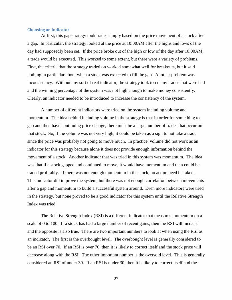
Choosing an Indicator
At first, this gap strategy took trades simply based on the price movement of a stock after
a gap. In particular, the strategy looked at the price at 10:00AM after the highs and lows of the
day had supposedly been set. If the price broke out of the high or low of the day after 10:00AM,
a trade would be executed. This worked to some extent, but there were a variety of problems.
First, the criteria that the strategy traded on worked somewhat well for breakouts, but it said
nothing in particular about when a stock was expected to fill the gap. Another problem was
inconsistency. Without any sort of real indicator, the strategy took too many trades that were bad
and the winning percentage of the system was not high enough to make money consistently.
Clearly, an indicator needed to be introduced to increase the consistency of the system.
A number of different indicators were tried on the system including volume and
momentum. The idea behind including volume in the strategy is that in order for something to
gap and then have continuing price change, there must be a large number of trades that occur on
that stock. So, if the volume was not very high, it could be taken as a sign to not take a trade
since the price was probably not going to move much. In practice, volume did not work as an
indicator for this strategy because alone it does not provide enough information behind the
movement of a stock. Another indicator that was tried in this system was momentum. The idea
was that if a stock gapped and continued to move, it would have momentum and then could be
traded profitably. If there was not enough momentum in the stock, no action need be taken.
This indicator did improve the system, but there was not enough correlation between movements
after a gap and momentum to build a successful system around. Even more indicators were tried
in the strategy, but none proved to be a good indicator for this system until the Relative Strength
Index was tried.
The Relative Strength Index (RSI) is a different indicator that measures momentum on a
scale of 0 to 100. If a stock has had a large number of recent gains, then the RSI will increase
and the opposite is also true. There are two important numbers to look at when using the RSI as
an indicator. The first is the overbought level. The overbought level is generally considered to
be an RSI over 70. If an RSI is over 70, then it is likely to correct itself and the stock price will
decrease along with the RSI. The other important number is the oversold level. This is generally
considered an RSI of under 30. If an RSI is under 30, then it is likely to correct itself and the
28
stock price will increase along with the RSI. But, the optimal overbought and oversold levels
may change from stock to stock and can be checked and adjusted by back testing, which will be
covered later.
When it came to picking an exit, the process was one of trial and error. Originally, the
strategy would exit after a gap was filled (if a gap fill was expected). For breakouts, the strategy
would only exit a position at the end of the day, or when profit targets or stop losses were met.
But, the strategy was missing out on potential profit if a stock filled the gap and then kept
moving in a favorable way for the strategy. Additionally, the strategy was not locking in profits
on breakouts that would turn around throughout the course of the day. So, after trying several
exit strategies, the one that worked the best in this system was an ATR exit strategy. This
strategy generates a stop order at the highest price since the entry of the trade minus a number of
average true ranges. The number of average true ranges can be optimized through back testing.
This exit worked well because as new higher prices are obtained, the stop order is scaled up,
which means that this type of exit leaves room for a more profitable trade, while still helping to
lock in some level of profits. There was also a stop loss on this strategy. This stop loss closed
any position that was losing more than one and a half percent of the equity risked.
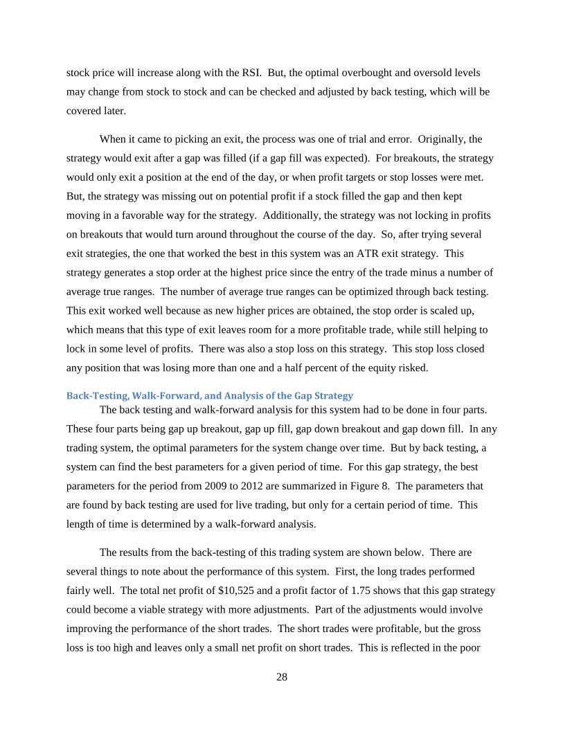
Back-Testing, Walk-Forward, and Analysis of the Gap Strategy
The back testing and walk-forward analysis for this system had to be done in four parts.
These four parts being gap up breakout, gap up fill, gap down breakout and gap down fill. In any
trading system, the optimal parameters for the system change over time. But by back testing, a
system can find the best parameters for a given period of time. For this gap strategy, the best
parameters for the period from 2009 to 2012 are summarized in Figure 8. The parameters that
are found by back testing are used for live trading, but only for a certain period of time. This
length of time is determined by a walk-forward analysis.
The results from the back-testing of this trading system are shown below. There are
several things to note about the performance of this system. First, the long trades performed
fairly well. The total net profit of $10,525 and a profit factor of 1.75 shows that this gap strategy
could become a viable strategy with more adjustments. Part of the adjustments would involve
improving the performance of the short trades. The short trades were profitable, but the gross
loss is too high and leaves only a small net profit on short trades. This is reflected in the poor

29
profit factor of 1.18. Other important statistics in this performance summary are the high
number of trades, which was expected of this system, and the maximum consecutive losing
trades of six. This is important because a system that does not lose a lot of consecutive trades is
psychologically easier to trade. The equity curve for the back-testing shows that there were a
few poorly performing periods for the system, but it continued to make profits over time.
Figure 7: BP Back-testing Performance Summary
Figure 8: BP Equity Curve

30
Figure 9: Gap Optimized Parameters
A walk-forward analysis is used to determine the best amount of historical data to use
when determining parameters for a trading system. It will also determine how long these
parameters can be used for before they need to be recalculated. For this system, four separate
walk-forward analyses needed to be used. The results are provided in Figure 9a through
Figure 9d. Of the four walk-forward tests, three were failures and only one was a pass. This
may seem discouraging, but there are some reasons why this may not be devastating news. First
of all, the gap system as a whole is made up of the four smaller strategies. But, it was not
possible to perform a walk-forward analysis on the system as a whole. Just because each smaller
strategy failed the walk-forward test that does not necessarily mean that the system as a whole
would fail a walk-forward analysis. The system as a whole would be more robust than each
individual strategy. Another reason why the walk-forward analysis may not have been
conclusive is because there may not have been enough tests in each walk-forward. The test may
not have been comprehensive enough to be conclusive.
BP CVS JPM
Gap Up Overbought 69 87 72
Gap Up Oversold 15 20 20
Gap Down Overbought 60 60 60
Gap Down Oversold 27 35 38
RSI Length 8 8 8
Number of ATR for
Trailing LX
7 7 7
ATR Length 8 8 8

31
Figure 10a: Walk-Forward Gap Up Longs (Top)
Figure 10b: Walk-Forward Gap Up Shorts (Bottom)
Figure 10c: Walk-Forward Gap Down Longs (Top)
Figure 10d: Walk-Forward Gap Down Shorts (Bottom)
Evaluating the System using Expectancy, Expectunity, and System Quality
There are three measurements of the effectiveness of a trading system that are used in this
paper. The three technical analysis methods that are used are expectancy, expectunity, and
system quality (Van Tharp Institute, 9 May 2014). The gap trading system was applied to three
stocks and then these measures were calculated for the system’s performance on each stock.
In any profitable trading system, a positive expectancy is necessary. Expectancy is a
measure of how much a system will make per dollar risked (Tharp 59). A positive expectancy
32
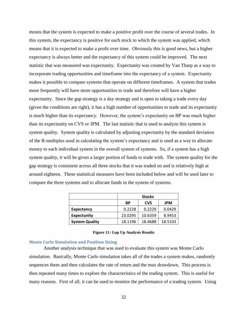
means that the system is expected to make a positive profit over the course of several trades. In
this system, the expectancy is positive for each stock to which the system was applied, which
means that it is expected to make a profit over time. Obviously this is good news, but a higher
expectancy is always better and the expectancy of this system could be improved. The next
statistic that was measured was expectunity. Expectunity was created by Van Tharp as a way to
incorporate trading opportunities and timeframe into the expectancy of a system. Expectunity
makes it possible to compare systems that operate on different timeframes. A system that trades
more frequently will have more opportunities to trade and therefore will have a higher
expectunity. Since the gap strategy is a day strategy and is open to taking a trade every day
(given the conditions are right), it has a high number of opportunities to trade and its expectunity
is much higher than its expectancy. However, the system’s expectunity on BP was much higher
than its expectunity on CVS or JPM. The last statistic that is used to analyze this system is
system quality. System quality is calculated by adjusting expectunity by the standard deviation
of the R-multiples used in calculating the system’s expectancy and is used as a way to allocate
money to each individual system in the overall system of systems. So, if a system has a high
system quality, it will be given a larger portion of funds to trade with. The system quality for the
gap strategy is consistent across all three stocks that it was traded on and is relatively high at
around eighteen. These statistical measures have been included below and will be used later to
compare the three systems and to allocate funds in the system of systems.
Figure 11: Gap Up Analysis Results
Monte Carlo Simulation and Position Sizing
Another analysis technique that was used to evaluate this system was Monte Carlo
simulation. Basically, Monte Carlo simulation takes all of the trades a system makes, randomly
sequences them and then calculates the rate of return and the max drawdown. This process is
then repeated many times to explore the characteristics of the trading system. This is useful for
many reasons. First of all, it can be used to monitor the performance of a trading system. Using
Stocks
BP CVS JPM
Expectancy 0.2228 0.2229 0.0429
Expectunity 23.0295 10.6359 8.9453
System Quality 18.1196 18.4688 18.5103

33
information from the trials of the Monte Carlo analysis, a 95% confidence interval can be created
for the drawdown of the system. In Figure 11a, the 95% confidence intervals are illustrated
along with the actual equity curve from back testing. From this analysis it can be determined
that there is 95% confidence that our rate of return will be at least 12.93% and that the max
drawdown will be at most 3.447%. Confidence intervals can also be created for future trades.
An example of this is Figure 11b. This is useful because if future trades are outside of the
predicted 95% confidence interval, it is an indication that the trading system needs to be adjusted
or even abandoned. Without confidence that the system is behaving normally, it does not make
sense to continue trading it. Figure 11b shows that this system stayed within our projected
confidence interval. This means that the system was behaving normally and could continue to be
traded. Position sizing strategy refers to how large a position will be taken throughout the course
of a trade (Van Tharp Institute, 9 May 2014). Fixed fractional position sizing is a position sizing
technique that scales the amount of money risked on each trade based on the total equity in a
trading account. So, if an account with $100,000 has a fixed fractional position sizing of 20%, it
will risk $20,000 on the next trade. If that trade goes well, and the account then has $110,000,
the next trade will risk $22,000. Position size also scales down if an account is losing money.
Using optimization with a different fixed fractional each time, the optimal fixed fraction can be
discovered. Using optimization, an equity curve using the optimal fixed fractional position
sizing was created and is included in Figure 11d. According to the simulation, the optimal fixed
fractional is one hundred percent. This means that the gap system had its best performance when
it risked all of its equity on each trade. This fixed fractional did significantly improve the equity
curve, but it is not wise for any trader to risk all of their equity on one trade.

34
Figure 12a: BP Monte Carlo Simulation with 95% Confidence Interval
Figure 12b: BP Monte Carlo 95% Confidence Interval Prediction

35
Figure 12c: BP Equity Curve Before Fixed Fractional Position Sizing
Figure 12d: BP Equity Curve After Fixed Fractional Position Sizing

36
Development and Analysis of the Trend Following Strategy There were two very similar strategies that were developed to trade Google and Facebook
but both strategies have slight differences based on the stock’s trend. It was observed that Google
very rarely deviated from a bull state which means that it was in a constant up trend. This makes
for a perfect situation to take long positions. The strategy used moving average crossovers long
entry and long exit as indicators. Facebook proved to be more volatile than Google. Due to this,
Facebook also used short entry and short exit indicators, aside from the longs. Also, as
previously mentioned, Google was traded using intra-day 120- minute bars while Facebook used
60 to 90- minute bars in order to account for slight volatility. Figures 12 and 13 present the
performance summaries for both stocks.
Figure 13: Facebook Back-Testing Performance Summary

37
The performance summary in Figure 12 shows the results of the trend following
strategy used to trade Facebook. Although the percent profitability is 50% and the number of
winning trades is equal to that of the losing trades, it is worth mentioning that the total net profit
is very strong at $11, 914.00 and a profit factor of 2.61 is favorable. Profit factor is another way
to measure the attractiveness of a trade set-up. It is calculated by dividing the historical net
profits by the historical net losses and a profit factor greater than one means that the strategy is
making money. The average winning trade for this strategy is also much higher than the average
losing trade.
Figure 14: Google Back-Testing Performance Summary

38
In the performance summary for Google (shown in Figure 13) one of the main values
worth noting is the quantity of losing trades versus winning trades. It can be inferred that there is
a noticeable amount of risk taken due to the quantity of losing trades observed above. Although
total net profit is high, gross loss must also be taken into account since more than $10,000 was
lost. Despite the percent profitability being below 50% and the number of losing trades
exceeding that of winning trades, it is still a profitable strategy with a strong profit factor of 2.33.
This means that although there were more losing trades, these were probably for small losses
cause by noise, but losses could have been much greater if not for a good exit strategy.
Development and Analysis of the Volatility Expansion Strategy After deciding to work with a volatility expansion system, the next step was to figure out
exactly how one worked. Luckily, TradeStation had an example system pre-built among four
different small strategies, all of which marked volatility expansion. Next, stocks needed to be
selected. To start off, Twitter seemed like a fine choice. It had been moving dramatically, so
using its volatility seemed like a strong venture. However, this proved not true on any bar length
– small bars caught all the noise, while longer bars missed most moves. Whether the system
made too many trades, many of which were not profitable, or it made too few trades, one thing
was true: the system was not making money. Twitter was not going to make money with this
idea, but maybe WalMart or Hess would. Using a volatility expansion strategy, both WalMart
and Hess were on the way to making profit, their profit factors only reached to about 1.09,
which, while profitable, will not make money very fast. Something new needed to be tried.
Shorting and short-covering proved to not be particularly profitable. In the interest of
pure profit, the shorting side of the strategy was removed. This also tied in to an idea not having
to owe anyone stocks or money, which adds the interest problem. However, V (Visa) traded very
well on the system and, as time went on, the system grew more and more into making V into the
most profitable stock for the system.
The current TradeStation codes prove ineffective in most cases. A 2002 November issue
of the Breakout Bulletin, which is a trading newsletter, proved to have a similar but more refined
strategy, designed to show the impact of a volatility filter. While the breakout function was
simple, it seemed much more self-integrated than the modular interchangeable codes of
TradeStation. As one may naturally expect, the integrated system, while only designed for an

39
example, proved a better quality. Although another result was, perhaps a bit counter intuitively,
the volatility filter sometimes proved more inhibitive than helpful. This could also be due to the
removal of context: the system was designed to trade the S&P 500 with $75 commission and
daily bars, while the current written strategy was using $7 commission and ten-minute bars on V.
It would be naturally expected that it would not quite perform as good as the reported results
shown in the magazine. In order to attempt to reproduce similar results, the system was switched
to daily bars. V instantly worked much better on such a timeframe, and such daily bars were kept
to the end of the project. However, optimizations of the strategy as written resulted in very few
trades, and in addition the profit factors proved either very poorly or scarily well. One such
optimization led to a profit factor of 643, but this proved to be a fluke and didn’t work for any
other timeframe other than the one it was back-tested for (Bryant, 20 April 2014).
The 2002 article system proved simple and relatively inefficient. One found in a February
2003 article proved much more complex. The first process was to remove the short and short-
cover mechanisms: these have always proven to be unreliable and much more trouble than they
are worth. Next in the list of alterations was to make into inputs any solid numbers. While 22 has
context in terms of average number of trading days in a month, replacing it with an AvData
would allow for further customization and optimization (Bryant, 24 April 2014).
After configuration of inputs and variables, the next step was to find more stocks on
which to trade the system. Most stock filters would provide the option to find high volume
(3,000,000 shares per day or higher) and smaller range betas (0.5 to 2). Many stocks popped up
even under this filter, so the filter for beta was converged to closer and closer towards V until it
led to a small, manageable list of stocks to test. Of those stocks, the best-proving ones were
BEAM and ADBE.
Technical Analysis of the System
For this project, the stocks chosen were Beam Inc. (BEAM), Adobe Systems
Incorporated (ADBE), and Visa (V).

40
How the system performs with BEAM
Figure 15a: BEAM Optimized Parameters
For the sake of reproducibility, these are the variables, which were described earlier, and
the initial capital that the system used. This back-testing included a commission of $10 per trade.
The $10 commission is unusual, given that most basic trading platforms have $7 commission.
However, TradeStation’s commission has occasionally been known to approach $10, and this
prepares for the worst. Besides, that means the system saves more money than it thought it would
spend, resulting indirectly in more net profit.

41
Figure 15b: BEAM Back-Testing Performance Summary
As noted here, on the trading interval used to test BEAM, it has made a 3.23 profit factor,
which means that, for every dollar lost in it, it has gained 3.23 dollars. Out of 150 trades, it won a
resounding 115 of them and lost 35 of them, accounting that 76.67% of its trades were profitable.
However, the timeframe was from 1/2/1998 to 12/31/2012, showing that it only took 150 trades
over about 15 years, an average of 10 trades per year. The select profit factor “removes the trades
further than standard deviations away from the average trade”, as such removing all the outliers.
(Select Profit Factor). Noting that, the Select profit Factor increases dramatically, with most of
the loss being removed. Meanwhile, the Adjusted Profit Factor “displays the amount made in
relation to the amount lost, for a worst case scenario during the specified period.” (Adjusted
Profit Factor). Even in this worst case scenario, the system still trades at a reasonable profit
factor level, vouching for the viability of the system.

42
Figure 15c: BEAM Efficiency
This chart shows the efficiency of each trade, going from -100 to 100. While one of the
trades is a huge hiccup and many trades approach zero efficiency, the average trade estimates
37.5% efficiency.
Figure 15d: BEAM Equity Curve

43
Perhaps one of these most important graphs is the Equity Curve. A perfect equity curve is
a straight line, meaning that every trade was perfectly executed. Such a system is likely not
possible, however it is the goal of every trading system to have a perfect equity curve. The curve
for this volatility expansion strategy takes a dip right at the beginning but is able to somewhat
manage a straight line after such a dip. This remarks hope for the system.
Figure 15e: BEAM Walk-Forward Cluster Analysis
The system works fine in its own time frame, but how is it projected to work outside of
its own time frame? For this, a Walk-Forward Optimization is in order. As shown by the above
graph, there is a small sideways T of PASS outside a PASS**. While the system passed under
the test provided at OOS% 15 and 25 Runs, it’s standing on a telephone pole with little support,
meaning that if the market shifts even by a small bit, this system’s viability could be devastated.
It is best to have a 9x9 square on this chart with the one in the middle being the most viable. On
such a note, a minor change in the market will not likely disrupt how the system works. These
results not only show that the system has a long way to go before it reaches it maximum profit,
but they also remark that the system is on the right track.

44
Figure 15f: BEAM Walk-Forward Results
On the block with the PASS**, it shows a result of all PASS or PASS** on this square.
These Walk-Forward settings will work tremendously while the market stays in a similar
arrangement to a pattern shown in the last 15 years of the market.
Figure 15g: BEAM System Quality Analysis
To calculate the expectancy, expectunity and system quality of this system, a function
called writetrades was used to transfer the data about trades that the system took into Excel
(shown in the Appendices section). The trade data was then used to calculate expectancy,
expectunity and system quality. The expectancy, or how much money the system expects to
make per trade, is 0.52004 when accounting for the average loss (the average scenario) and
.017292 when accounting for the worst loss in the system’s data set of trades, so as to account for
a worst case scenario. A negative expectancy shows invalidity of a system, due to it indicating
that, over the long run, the system loses money. While a smaller expectancy is worse than a
larger expectancy given the same number of trades and time frame, a smaller expectancy may be
an indication of either a poor system or a scalping system, a trading system designed to make

45
many trades each with a small profit. To account for this, opportunities of trades per year gets
accounted. As mentioned previously, the system makes about 10 trades per year. The expectunity
is an annualized expectancy, meaning it is used to analyze money made per year. Here, the result
is 5.302081 on an average year or 0.176299 in the worst year possible.
The last statistic calculated was system quality, which simply is determined by the
product of the average winning trade and the square root of the number of trades, divided by the
standard deviation of the winning trades. Given the numbers accounted here, the system quality
is determined to be 11.00434. This statistic was used for money allocation for the system of
systems.
How the system performs with V
Figure 16a: V Optimized Parameters

46
Figure 16b: V Back-Testing Performance Summary
A profit factor of 4.78 showed great promise. The select profit factor of 62.60 showed
potential of very high gains, while the adjusted profit factor being 3.55 showed that, no matter
what, V would make a lot of money on this strategy.
Figure 16c: V Efficiency

47
Unfortunately, the efficiency appeared to be under 37.5%. However, there seemed to only
be one big outlier.
Figure 16d: V Equity Curve
The equity curve isn’t perfect, particularly from about 40 to 80. The line proved a bit
rigid. This carries hope but still is far from an ideal.
Figure 16e: Walk-Forward Cluster Analysis
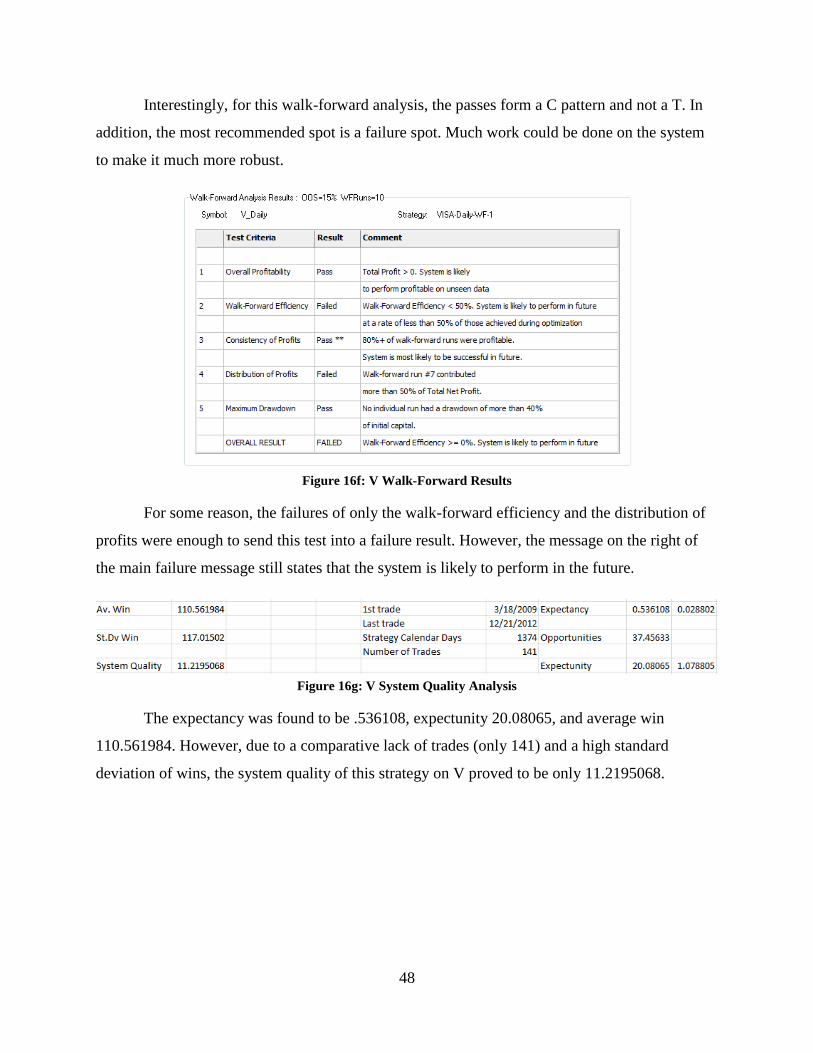
48
Interestingly, for this walk-forward analysis, the passes form a C pattern and not a T. In
addition, the most recommended spot is a failure spot. Much work could be done on the system
to make it much more robust.
Figure 16f: V Walk-Forward Results
For some reason, the failures of only the walk-forward efficiency and the distribution of
profits were enough to send this test into a failure result. However, the message on the right of
the main failure message still states that the system is likely to perform in the future.
Figure 16g: V System Quality Analysis
The expectancy was found to be .536108, expectunity 20.08065, and average win
110.561984. However, due to a comparative lack of trades (only 141) and a high standard
deviation of wins, the system quality of this strategy on V proved to be only 11.2195068.

49
How the system performs with ADBE
Figure 17a: ADBE Optimized Parameters
As mentioned in the BEAM section, these are the variables used for the rest of the
graphs. As a reminder, with commissions less than $10, the system can be expected to work
better.
Figure 17b: ADBE Back-Testing Performance Summary

50
Here, the profit factor is much lower than with BEAM at only 2.08. However, its select
profit factor doesn’t expand very largely, nor does its adjusted profit factor drop much. This
proves much more stability in its patterns.
Figure 17c: ADBE Efficiency
Even accounting for the super-low outliers in this example, the efficiency still proves
around 37.5% at a glance.

51
Figure 17d: ADBE Equity Curve
This equity curve has quite some trouble starting up. After trade number 140, however,
the system really picked up and, after the next twenty, started on an upward slope. Even so, the
system will not look convincing to most.
Figure 17e: ADBE Walk-Forward Cluster Analysis

52
And this chart is very disappointing – not a single pass in this chart. At this sign of a
chart, most professionals would stop the process here and work a different stock or even just
remove the entire strategy from their repertoire.
Figure 17f: ADBE Walk-Forward Results
However, even that whole grid of failure had a silver lining. Overall Profitability analysis
states that the system is likely to perform profitable on unseen data and Consistency of Profits
analysis states that the profits are consistent.
Figure 17g: ADBE System Quality Analysis
All of expectancy, expectunity, and average win are small (0.069119, 0.852573, and
57.93233, respectively), yet it has the largest system quality from among all three (in this case,
16.01992). Why would such be, after all the previous analysis? The answer lies in the
consistency. While this volatility expansion strategy may deliver small amounts of money with
ADBE, it does so more consistently than it does with BEAM and V.

53
System Comparison and System of Systems Analysis From the analysis that was done on all three systems, we were able to find three
important statistical values for each system. These three values are expectancy, expectunity, and
system quality. These three values were found for the three different stocks that each system
was traded on and are provided in Figure 17. One thing that is notable is the difference in
expectancy and expectunity between the three systems. The expectancy for the gap strategy is
generally lower than that of the volatility strategy. This may be due to the fact that the gap
strategy works on a shorter timeframe than the volatility system. This leaves less time for the
trade to make profits and thus a lower expectancy. However, since there are many opportunities
for trades in this gap strategy, its expectunity measures more favorably relative to the volatility
expansion system. A similar pattern occurred with the trend-following system. Since this
system was designed to trade on a shorter timeframe than a traditional trend-following system, it
had many opportunities to trade and had very good expectunity values. In fact, this system had
the most consistent expectunity across its stocks. But, the last statistic that was calculated,
system quality, was the statistical value that determined how much money would be allocated to
each system for trading.
System quality is often used as a way to compare trading systems that operate on
different indicators, timeframes and other criteria. System quality is calculated by taking the
square root of the number of trades, multiplying by the average winning trade and then dividing
by the standard deviation of winning trades. This takes not only the size of winning trades into
account, but also the consistency of the size of winning trades. In this system of systems, the gap
strategy had the most consistent and highest system qualities, which is an indication that the
systems winning trades are not only sizable, but consistent. When allocating money to a system
of systems, comparing system quality is a good indicator of how much money should be invested
into each system. For this system of systems, a weighted average of system quality was used to
allocate money. Therefore, the percentage of total system quality that each system contributed
was also the percentage of money that they were given. Since the total amount of simulated
trading money between the three traders was $300,000, that total was split up by the percentages
given in Figure 17.

54
Figure 18: System Quality Comparison Table
Volatility Gap Trend-Following
V ADBE BEAM BP CVS JPM GOOG FB GOLD
Expectancy 0.5361 0.0691 0.5200 0.2228 0.2229 0.0429 0.7402 0.2850 0.0968
Expectunity 20.0807 0.8526 5.3021 23.0295 10.6359 8.9453 23.1856 17.0862 19.3593
System Quality 11.2195 16.0199 11.0043 18.1196 18.4688 18.5103 16.9234 10.3490 11.3284
% Money Allocated 8.5033 12.1415 8.3402 13.7329 13.9976 14.0290 12.8263 7.8435 8.5858
Amount of Money $25,510 $36,425 $25,021 $41,199 $41,993 $42,087 $38,479 $23,531 $25,757
Conclusions and Looking Forward The gap strategy that was developed for this project is probably not ready to be traded
using real money. The system had a positive expectancy, but the rate of return was just not high
enough to make it worthwhile to trade. An investor would be better off investing their money in
an exchange traded fund that mimics the S&P 500. The S&P 500 had a return on investment of
15.89% in 2012 and 32.15% in 2013 (New York University, 9 May 2014). These returns are
higher than the returns of the gap strategy and the exchange traded fund is less risky than the gap
strategy. Therefore, there is no incentive to trade the gap strategy. Given more time, one of the
first things that would be improved about the system is its exit rules. The exit rules that were
used are not very impressive based on results, but they are the best rules that were found for the
system. With more time, more exit rules could be tested and the system would be vastly
improved. An alternative way to improve the system is to find a better stock to trade. BP does
gap frequently and its behavior is predictable, but its price does not move much in any given day,
which means that a lot of money needs to be invested per trade to really see a good return. By
picking a different stock that is perhaps more volatile during the day, higher profits could be
earned without risking too much money on any given trade.
The purpose of the trend following strategy that was developed for this system of systems
was fulfilled but only to a certain extent. Typically, trend following strategies are developed to
take advantage of big market swings and will only make about five to seven trades over the
course of a year. The trend following strategy for this project was designed to increase the
number of trades and was used with intra-day bars rather than monthly or yearly bars in an

55
attempt to avoid noise. The number of trades definitely increased and both strategies for Google
and Facebook were profitable. It can be observed though, that noise affected the profitability of
the strategy used to trade Google, which suggests that, for future projects, more research should
be conducted on noise and how noise affects the market. Also, more experimentation should be
conducted with exit strategies and a wider range of trending stocks.
Overall, the volatility expansion system proved moderately well in current testing, and,
even relative to the other systems in the overall system, it held its own very well. However,
overall for future testing, the figures show that the system isn’t quite robust enough yet. While it
could be traded and one could make money using it, it may not generate the alpha needed
consistently enough and without any worries to the prospective user of the system to overall be
more worthwhile to said prospective user. However, since the code is so simple, a great number
of modifications could be made to the code to improve it. The most important one to tackle
would likely to be to reinstate and rework the shorting and cover code. While such code was
found detrimental for these tests, removing it proved overall detrimental for the final tests of the
system. To further experiment, one could try adjusting the role of the volatility to play a bigger
role than just a breakout measurer for entries and exits. A large quirk in the code that could cut
down profits is the “exit after 2 bars” strategy. While this gets the strategy out when the breakout
usually ends, what if it keeps going? A trailing stop could in theory be used instead, but it could
also reduce the gains of some profitable trades. Finally, the last avenue to check out from
observations here was that ADBE took a two-year trade. An inactivity stop could prove reliable
to ensure such does not happen, but at the same time, offers high chance of failure. Such a
parameter for how many bars until exit could probably be optimized as well.
The overall system of systems achieved its goal. By allocating money to several unique
strategies and stocks, the system became more robust and consistent. Based on how the money
was allocated to each individual system, an overall expectancy and expectunity was calculated.
The overall expectancy of this system of systems is 0.29075 and the overall expectunity is
14.1357. As designed, the overall system of systems sacrifices higher returns for consistency
and robustness. If one individual strategy is performing poorly, the other systems will balance
this loss out. With additional time, the next step in this project would have been to further
analyze the system of systems to get a better understanding of how the systems worked together

56
compared to how they work individually. This could include a Monte Carlo simulation taking
into account all trades of the system of systems to better understand the expected performance of
the system. Something that was discovered during the completion of this project was that in a
system of systems, it is important to keep the systems diverse to avoid failure during poor
markets. In other words, if two systems are too much alike, they will be affected by the same
news and same market trends. In order to diversify systems, a trading system developer must
have a comprehensive knowledge of how markets relate and move in relation to one another.

57
Works Cited “A Gap Strategy for the E-mini S&P”. Seven Trading Systems.16 July 2010. Web. 10 January
2014. <http://seventradingsystems.com/day-trade-strategy.php>.
"Adjusted Profit Factor." Adjusted Profit Factor (Report Field). TradeStation. Web. 16 Apr.
2014.<http://help.tradestation.com/08_08/tradestationhelp/mergedprojects/spr_topics/rep
ort/adjusted_profit_factor__strategy_performance_report_.htm>.
“Annual Returns on Stock, T.Bonds and T.Bills: 1928 – Current”. New York University. Web. 9
May 2014.
<http://pages.stern.nyu.edu/~adamodar/New_Home_Page/datafile/histretSP.html>.
"Average True Range." Average True Range. TradeStation. Web. 20 Apr. 2014.
<http://help.tradestation.com/09_00/tradestationhelp/commentary/average_true_range.ht
m>.
Bollinger, John. "Bollinger Bands Introduction." BollingerBands. Bollinger Capital
Management, Inc.. Web. 7 Apr 2014. <http://www.bollingerbands.com/>.
Bollinger, John. Bollinger Bands Introduction. N.d. Photograph. BollingerBand. Web. 26 Apr
2014. <http://www.bollingerbands.com/>.
Bryant, Mike. "Breakout Bulletin - February 2003." Breakout Bulletin - February 2003.
Breakout Futures, Feb. 2003. Web. 20 Apr. 2014.
<http://www.adaptrade.com/BreakoutFutures/Newsletters/Newsletter0203.htm>.
Bryant, Mike. "Breakout Bulletin - November 2002." Breakout Bulletin - November 2002.
Breakout Futures. Web. 25 Apr. 2014.
<http://www.adaptrade.com/BreakoutFutures/Newsletters/Newsletter1102.htm>.
Cruset, José. "Analysis of Trend Following Systems." . N.p., n.d. Web. 3 Apr 2014.
<http://www.cruset.com/systemtrader/download/trendfollowing.pdf>.
F., Andreas. "Trading System Rules." Following The Trend. N.p., 1 Jan. 2014. Web. 7 Apr.
2014. <http://www.followingthetrend.com/the-trading-system/trading-system-rules/>.

58
“Gaps and Gap Analysis”. StockCharts. Web. 6 April 2014.
<http://stockcharts.com/school/doku.php?id=chart_school:chart_analysis:gaps_and_gap_
analysi>.
“Indicators”. TradeStation. Web. 10 April 2014.
<http://www.tradestation.com/en/education/university/markets-and-trading-resource-
center/articles/technical-analysis/indicators>.
Kennedy, Rory. “Autotrading vs. Manual Trading”. Wealth Creator. Web. 9 April 2014.
<http://www.wealthcreator.com.au/invest/advice/autotrading-vs.-manual-trading>.
Mitchell, Todd. “In Search of the Holy Grail Trading System”. Trading Concepts. 10 April 2013.
Web. 8 April 2014. <http://www.tradingconceptsinc.com/5564/search-holy-grail-trading-
system/>.
“MONEX Group Releases Full Financial Results For H1 Of Fiscal Year: Flying Start Curtailed.”
Forex Magnates. Chart. 31 Oct 2014. Web. 1 May
2014.<http://forexmagnates.com/monex-group-releases-full-financial-results-for-h1-of-
fiscal-year-flying-start-curtailed/>.
"Moving Average Crossovers." Online Trading Concepts. OnlineTradingConcepts.com, n.d.
Web. 3 Apr 2014.
<http://www.onlinetradingconcepts.com/TechnicalAnalysis/MASimple2.html>.
Mulloy, Patrick. Triple Exponential Moving Average (TEMA) Technical Indicator. N.d. Chart.
Trade Forex TradingWeb. 22 Apr 2014.
<http://www.tradeforextrading.com/index.php/tema-moving-average>.
Nathan, Narendra. “How to Use RSI Indicator to take Decisions on Buying and Selling Stocks”.
8 April 2013. Web. 9 April 2014. <http://articles.economictimes.indiatimes.com/2013-
04-08/news/38374193_1_rsi-overbought-zone-swing>.
“Relative Strength Index”. StockCharts. Web. 7 April 2014.
<http://stockcharts.com/school/doku.php?id=chart_school:technical_indicators:relative_s
trength_in>.

59
Schlossberg, Boris. “Top 7 Questions About Currency Trading Answered”. Investopedia. 7 May
2014. Web. 8 May 2014.
<http://www.investopedia.com/articles/forex/06/sevenfxfaqs.asp>.
"Select Profit Factor." Select Profit Factor (Report Field). TradeStation. Web. 16 Apr. 2014.
<http://help.tradestation.com/08_08/tradestationhelp/mergedprojects/spr_topics/report/sel
ect_profit_factor__strategy_performance_report_.htm>.
“Strategies for Trading Relative Strength Index- RSI Technical Indicator”. Web. 6 April 2014.
<http://www.stock-market-strategy.com/relative-strength-index-rsi/>.
Tharp, Van. Trade Your Way to Financial Freedom. New York: McGraw-Hill, 1998. Print.
Thygesen, Philip. “Relative Strength Index – RSI”. Stock Market Strategy. 9 Arpil 2010. Web. 4
April 2014. < http://www.stock-market-strategy.com/relative-strength-index-rsi/>.
"True Range." True Range. TradeStation. Web. 20 Apr. 2014.
<http://help.tradestation.com/09_01/tradestationhelp/charting_definitions/true_range.htm
>.
Tucci, Nathan. “Manual Trading vs Automated Trading”. Winner’s Edge Trading. 1 June 2012.
Web. 7 April 2014. <http://www.winnersedgetrading.com/manual-trading-or-automated-
trading/>.
“Van Tharp’s Glossary of Terms”. Van Tharp Institute. Web. 9 May 2014.
<http://www.vantharp.com/glossary.asp>.
“What is a 401(k)?”. Wall Street Journal. Web. 17 April 2014. <http://guides.wsj.com/personal-
finance/retirement/what-is-a-401k/>.
Wyckoff, Jim. “Kaufman: Multiple Trading Methods and Market ‘Noise’”. Acton Forex. Web. 6
April 2014. <http://www.actionforex.com/articles-library/general-trading-
articles/kaufman:-multiple-trading-methods-and-market-%22noise%22-
2007112632430/>.

60
Appendices
Gap Strategy Code
Gap Up
Inputs: Price(Low), Length(14), Oversold(30), Overbought(70), psize(500), ProfitTargetPct( .10
), { pass in 0 if you don't want a profit target }
StopLossPct( .05 ); { pass in 0 if you don't want a stop loss }
Variables: JNRSI(0);
JNRSI = RSI(Price, Length);
If OpenD(0)>HighD(1) and entriestoday(date)=0
and time <1000
and High<OpenD(0) and High>LowD(1)
And JNRSI crosses under Overbought
Then sellshort psize contracts next bar at market;
If OpenD(0)> HighD(1) and entriestoday(date)=0
And time >1000 and time < 1010
And JNRSI>Oversold
And High>High[1]
Then buy psize contracts next bar at market;
SetStopShare ;
if MarketPosition <> 0 then { set regular profit-target and stop-loss }
begin
if ProfitTargetPct > 0 then
SetProfitTarget( EntryPrice * ProfitTargetPct ) ;
if StopLossPct > 0 then
SetStopLoss( EntryPrice * StopLossPct ) ;
end
else { set entry-bar profit-target and stop-loss }
begin
if ProfitTargetPct > 0 then
SetProfitTarget( Close * ProfitTargetPct ) ;
if StopLossPct > 0 then
SetStopLoss( Close * StopLossPct ) ;
end ;
SetExitOnClose ;

61
Gap Down
Inputs: Price(Low), Length(14), Oversold(30), Overbought(70), psize(500), ProfitTargetPct( .10
), { pass in 0 if you don't want a profit target }
StopLossPct( .05 ) ; { pass in 0 if you don't want a stop loss }
Variables: JNRSI(0);
JNRSI = RSI(Price, Length);
If OpenD(0)<LowD(1) and entriestoday(date)=0
and time <1030
and High>OpenD(0) and High<LowD(1)
And JNRSI crosses over Oversold
Then buy psize contracts next bar at market;
If OpenD(0)<LowD(1) and entriestoday(date)=0
And time>1030
And JNRSI < Oversold
{and High<OpenD(0)} And High<High[1] and High[1]<High[2]
Then sellshort psize contracts next bar at market;
SetStopShare ;
if MarketPosition <> 0 then { set regular profit-target and stop-loss }
begin
if ProfitTargetPct > 0 then
SetProfitTarget( EntryPrice * ProfitTargetPct ) ;
if StopLossPct > 0 then
SetStopLoss( EntryPrice * StopLossPct ) ;
end
else { set entry-bar profit-target and stop-loss }
begin
if ProfitTargetPct > 0 then
SetProfitTarget( Close * ProfitTargetPct ) ;
if StopLossPct > 0 then
SetStopLoss( Close * StopLossPct ) ;
end ;

62
Trend Following Strategy Code
Facebook Strategy
{ Buys if Price crosses over Avg and then stays above Avg for one or more bars }
inputs: Price( Close ), Length( 9 ), ConfirmBars( 1 ) ;
variables: Counter( 0 ), Avg( 0 ) ;
Avg = AverageFC( Price, Length ) ;
if Price > Avg then
Counter = Counter + 1
else
Counter = 0 ;
if CurrentBar > ConfirmBars and Counter = ConfirmBars then
{ CB > ConfirmBars check used to avoid spurious cross confirmation
at CB = ConfirmBars }
Buy ( "MACrossLE" ) next bar at market ;
if CurrentBar > 1 and Price crosses under Avg then
{ CB > 1 check used to avoid spurious cross confirmation at CB = 1 }
Sell ( "MACrossLX" ) next bar at market ;

63
Google Strategy
{ Buys if Price crosses over Avg and then stays above Avg for one or more bars }
inputs: Price( Close ), Length( 9 ), ConfirmBars( 1 ) ;
variables: Counter( 0 ), Avg( 0 ) ;
Avg = AverageFC( Price, Length ) ;
if Price > Avg then
Counter = Counter + 1
else
Counter = 0 ;
if CurrentBar > ConfirmBars and Counter = ConfirmBars then
{ CB > ConfirmBars check used to avoid spurious cross confirmation
at CB = ConfirmBars }
Buy ( "MACrossLE" ) next bar at market ;
if CurrentBar > 1 and Price crosses under Avg then
{ CB > 1 check used to avoid spurious cross confirmation at CB = 1 }
Sell ( "MACrossLX" ) next bar at market ;
if Price < AverageFC( Price, Length ) then
Counter = Counter + 1
else
Counter = 0 ;
if CurrentBar > ConfirmBars and Counter = ConfirmBars then
{ CB > ConfirmBars check used to avoid spurious cross confirmation
at CB = ConfirmBars }
Sell Short ( "MACrossSE" ) next bar at market ;
if CurrentBar > 1 and Price crosses over Avg then
{ CB > 1 check used to avoid spurious cross confirmation at CB = 1 }
Buy To Cover ( "MACrossSX" ) next bar at market ;
{ ** Copyright (c) 2001 - 2010 TradeStation Technologies, Inc. All rights reserved. **
** TradeStation reserves the right to modify or overwrite this strategy component
with each release. ** }

64
Volatility Expansion Strategy Code Input: FrLv0 (.8), {Breakout fraction, Low vol, longs}
FrLv1 (0.3), {Breakout fraction, high vol, longs}
{FrSv0 (.8), {breakout fraction, Low vol, shorts}
FrSv1 (0.3), {breakout fraction, high vol, shorts}}
MMFrL (2.0), {Volatility multiplier For exit, longs}
{MMFrS (2.0), {Volatility multiplier for exit, shorts}}
V0 (16), {Low volatility}
V1 (30), {high volatility}
AvData (22); {number of bar to look back in average true range}
Var: ATR (0), {Average true range}
ML (0), {Slope of B/O fraction curve, longs}
BL (0), {y-intercept, longs}
{MS (0), {slope of b/O fraction curve, shorts}
BS (0), {y-intercept, shorts}}
FrL (0); {Entry fraction For longs}
{FrS (0); {Entry fraction For shorts}}
ATR = Average(TrueRange, AvData);
ML = (FrLv1 - FrLv0)/(V1 - V0);
BL = FrLv0 - ML * V0;
{MS = (FrSv1 - FrSv0)/(V1 - V0);
BS = FrSv0 - MS * V0;}
FrL = ML * ATR + BL;
{FrS = MS * ATR + BS;}
Buy next bar at H + FrL * ATR stop;
{Sell short next bar at L - FrS * ATR stop;}
If MarketPosition = 1 and C > EntryPrice and BarsSinceEntry >= 1 then
Sell this bar at close;
{If MarketPosition = -1 and C < EntryPrice and BarsSinceEntry >= 1 then
Buy to cover this bar at close;}
If MarketPosition = 1 then
Sell next bar at EntryPrice - MMFrL * ATR stop;
{If MarketPosition = -1 then
Buy to Cover next bar at EntryPrice + MMFrS * ATR stop;}