Stock Price Volatility and Patent Citation Dynamics:

the case of the pharmaceutical industry

*Mariana Mazzucato (Open University)

**Massimiliano Tancioni

(University of Rome)

Open University Economics working paper 2006-55

Preliminary draft, please do not quote without permission of the authors

Paper to be presented at the IKD/DIME conference on Policy Implications of Recent Advances in the Economics of Innovation and Industry

Dynamics, (London, Dec. 15-16, 2006)

Abstract

Recent finance literature highlights the role of technological change in increasing firm specific and aggregate stock price volatility (Campbell et al. 2001, Shiller 2000, Pastor and Veronesi 2005). Yet innovation data is not used in these analyses, leaving the direct relationship between innovation and volatility untested. Our aim is to investigate more closely the relationship between stock price volatility and innovation using firm level patent citation data. The analysis builds on the empirical work by Mazzucato (2002; 2003) where it is found that stock price volatility is highest during periods in the industry life-cycle when innovation (measured at the industry level) is the most ‘competence-destroying’. Here we ask whether firms which invest more in innovation (more R&D and more patents) and/or which have ‘more important’ innovations (patents with more citations) experience more volatility. We focus the analysis on firms in the pharmaceutical and biotechnology industries between 1974 and 1999. Results suggest that there is a positive and significant relationship between idiosyncratic risk, R&D intensity and the various patent related measures. Preliminary support is also found for the ‘rational bubble’ hypothesis linking both the level and volatility of stock prices to innovation.

Key words: Idiosyncratic Risk; Volatility; Technological Change; Industry Life-Cycle.

JEL Classification G12 (Asset Pricing); 030 (Technological Change). *Econ. Dept, Open University, Walton Hall, Milton Keynes, MK7 6AA, UK, m.mazzucato@open.ac.uk ** Econ. Dept, University of Rome La Sapienza, massimilano.tancioni@uniroma1.it Mazzucato acknowledges support from a British Academy Grant (Firm growth dynamics during different knowledge regimes) as well as support from the ESRC Innogen centre. Comments from participants at various seminars and conferences are also appreciated, including the 2006 IKD-DIME workshop in London, a seminar at CESPRI-Bocconi, and the CERF Cambridge workshop on ‘Technology and Bubbles’. All errors remain our own.

1

1. Introduction

In recent years there has been increased attention, by both the economics profession

and the popular press, on the topic of stock price volatility. Interest peaked after the ‘New

Economy’ period when many high-tech stocks that were considered overvalued experienced

a large drop in their share price. But still now there persists the idea that the ‘knowledge

economy’ (less unfashionable a term than the New Economy), has resulted in greater

volatility, especially of small innovative firms which tend to go public earlier in their life-cycle

than in previous times.

Yet, in reality, there has been no trend increase of aggregate stock price volatility

(Schwert 1989; 2002). Particular periods have been characterized by high volatility, such as

the 1970’s and the 1990’s, but the increase has not persisted. Firm specific volatility has, on

the other hand, experienced a trend increase over the last 40 years (Campbell et al. 2001).

Various works have highlighted technological change as one of the key factors responsible

for this increase in firm specific risk, as well as the periodic increases of aggregate stock

price volatility. For example, Shiller’s work (2000) has shown that ‘excess volatility’, i.e. the

degree to which stock prices are more volatile than underlying fundamentals, is highest in

periods of technological revolutions when uncertainty is greatest. Campbell et al. (2001) find

that firm level idiosyncratic risk, i.e. firm specific volatility (as opposed to industry specific or

market level), has risen since the 1960’s and claim that this might be due to the effect of new

technologies, especially those related to the ‘IT’ revolution, as well as the fact that small firms

tend now to go public earlier in their life-cycle when their future prospects are more

uncertain. And Pastor and Veronesi (2004) claim that the reason that high tech firms have

prices that appear unjustifiably high (at the beginning of a ‘bubble’) is not due to irrationality,

but due to the effect that new technology has on the uncertainty about a firm’s average future

profits. The basic idea behind all these works (reviewed further below) is that innovation,

especially when ‘radical’, leads to high uncertainty hence more volatility.

Yet none of these studies actually use innovation data. Innovation is eluded to (e.g.

the ‘IT revolution’, the New Economy, radical change) but not measured, especially not at the

firm or industry level1. The aim of our paper is to better understand the dynamics of stock

price volatility by seeing whether we can in fact find evidence that stock price volatility is

related to firm level innovation. That is, we do not assume that volatility is a sign of greater

uncertainty due to underlying innovation but instead empirically test for this very relationship.

1 Of the above cited authors, Shiller (2000) comes closest to considering the impact of technology by looking at excess volatility during the course of technological revolutions.

2

The paper builds on our previous work (Mazzucato and Semmler 1999; Mazzucato

2002; 2003) where it is found that excess volatility and idiosyncratic risk are highest in

periods of the industry life-cycle when innovation is the most ‘radical’. However, while there

we measured innovation at the industry level (e.g. through a quality index derived from

hedonic prices), in the current paper we go a step further in linking innovation to volatility by

using firm level patent data. The productivity literature on market value and innovation has

already established a positive relationship between a firm’s market value, its R&D intensity

and its citation weighted patents (Griliches 1981; Pakes 1985; Hall 1993, Hall, Jaffe and

Trajtenberg 2005). Here we see whether this type of data can also help us better understand

volatility dynamics which, as argued above, have not been studied in light of firm specific

innovation dynamics.

Both Frank Knight (1921) and John Maynard Keynes (1973), who distinguished ‘risk’

from ‘uncertainty’, used technological innovation as an example of true uncertainty which

cannot be calculated via probabilities like risk2. We start from the assumption that patents

that are “more important” are those that are the most uncertain due to the way they challenge

the status quo, more so at least than incremental innovations (Tushman and Anderson

1986). We use citation weighted patents as a proxy for the ‘importance’ of an innovation and

see whether firms with more ‘important’ innovations experience more volatility. Specifically,

we test for the relationship between firm level idiosyncratic risk and the following innovation

variables: R&D intensity, patent counts, and patents weighted by their citations. We also

look at the impact of these variables on the level of price-earnings as this relationship lies at

the core of the ‘rational bubble’ hypothesis where both the level and volatility of stock prices

are related to the uncertainty regarding a firm’s average future profits (Pastor and Veronesi

2004; 2005).

As in our previous work, we focus our study on one particular sector so that we can

better relate stock price dynamics to the changing character and intensity of innovation over

the industry life-cycle (Gort and Klepper 1982). The biotechnology and pharmaceutical

industries (from now on biotech and pharma) are particularly interesting to study in this

regard due to their high rates of patenting and R&D intensity (providing us with ample

innovation data to study), and due to the way that the search process for innovations has

changed over the last half century (as documented in Gambardella [1995], Henderson et al.

2 “The practical difference between the two categories, risk and uncertainty, is that in the former the distribution of the outcome in a group of instances is known (either from calculation a priori or from statistics of past experience). While in the case of uncertainty that is not true, the reason being in general that it is impossible to form a group of instances, because the situation dealt with is in a high degree unique…” (Knight, 1921, p. 232-233)

3

[1999]) — motivating us to also ask whether the relationship between innovation and volatility

has co-evolved with such transformations.

Our analysis is carried out in 3 stages. We first see whether we can replicate the

results found in the market value (Tobin’s q) and innovation literature (Griliches, 1981; Hall,

Jaffe and Trajtenberg 2005 from now on HJT) using flow rather than stock variables

(cumulative and depreciated), since in the case of volatility it is the latest ‘news’ that is

relevant. Second, we test for a statistical relationship between idiosyncratic risk and these

innovation variables in order to explore the hypothesis that technology is the source of the

increase in firm specific risk (as suggested but not tested in Campbell et al. [2001], and

Shiller [2000]). Third, we test the ‘rational bubble’ hypothesis in Pastor and Veronesi (2004)

by exploring the relationship between the level of price-earnings (P/E) and the innovation

variables, as well as the direct relationship between idiosyncratic risk and P/E.

Our results provide preliminary evidence that there is indeed a positive and significant

relationship between firm specific volatility and firm level innovation. We find that both

idiosyncratic risk and the level of price earnings are significantly related to R&D intensity, and

to the various patent related measures used in the analysis. We also find a positive

relationship between these innovation measures and the level of price-earnings, as is

predicted by the ‘rational bubble’ hypothesis. We pay particular attention to the lag structure

of the independent variables as this provides information on the speed at which the market

reacts to news regarding innovation. In this regard it appears that the lag on innovation

outputs (patents) is lower than that on inputs (R&D), and also that the lags for biotech are

lower than those in pharma, suggesting that the market reacts more quickly to innovation in

newer segments of the sector.

The rest of the paper is organized as follows. Section 2 reviews the literature on

innovation and stock prices; Section 3 discusses the data used and the variables

constructed; Section 4 provides descriptive statistics and a discussion of the model selection

criteria; Section 5 presents the results and Section 6 concludes.

2. Innovation and Stock Prices (level vs. volatility): a quick review

Uncertainty in finance models refers to how expectations about a firm’s future growth

affects its market valuation (Campbell, Lo and McKinley 19973). Both Knight (1921) and

3 “The starting point for any financial model is the uncertainty facing investors, and the substance of every financial model involves the impact of uncertainty on the behaviour of investors, and ultimately, on market prices.” (Campbell, Lo and MacKinlay, 1997)

4

Keynes (1973) highlighted the way that technological innovation is an example of true

uncertainty, which cannot be calculated via probabilities like risk. Yet, even though a firm’s

investment in technological change is a major determinant of its (potential) future growth, few

finance models link stock price dynamics to innovation variables at the level of the firm and

industry. The few studies that do relate stock price dynamics to innovation, do so mainly by

linking changes in the stock price level to innovation, rather than linking changes in volatility

of stock prices to innovation. This is ironic given that it is especially the volatility of stock

prices, more than their level, which should be related to ‘news’ on changes in technology. In

this section we review the literature that relates stock price dynamics to innovation, dividing it

between those contributions that focus on the level of stock returns (2.1), and those that

focus on the volatility of stock returns (2.2)—neither one using innovation data—and then our

own contributions which have studied volatility dynamics using industry innovation data (2.3).

The rest of the paper is then dedicated to studying volatility dynamics using firm level

innovation data.

2.1 Innovation and stock prices (level)

Studies that link the level of stock prices to innovation come principally from the

applied industrial economics literature which studies innovation and stock prices during the

industry life-cycle (e.g. Jovanovic and MacDonald 1994; Jovanovic and Greenwood 1999;

Mazzucato and Semmler 1999) and the productivity literature on market value (Tobin’s q)

and patents (e.g. Griliches 1981; Hall, Jaffe and Trajtenberg 2005 from now on HJT).

Jovanovic and MacDonald (1994) make predictions concerning the evolution of the

average industry stock price level around the “shakeout” period of the industry life-cycle.

They predict that just before the shakeout occurs the average stock price will fall because the

new innovation precipitates a fall in product price which is bad news for incumbents. Building

on this work, Jovanovic and Greenwood (1999) develop a model in which innovation causes

new capital to destroy old capital (with a lag) and since it is primarily incumbents who are

(initially) quoted on the stock market, innovations by new start-ups cause the stock market to

decline immediately since rational investors with perfect foresight foresee the future damage

to old capital. In a study of the US auto industry (1899-1998), Mazzucato and Semmler

(1999) also relate the dynamics of the average industry stock price to the dynamics of the

industry ‘shakeout’.

5

Another body of literature that connects stock prices to innovation is that on the

relationship between a firm’s market value, its stock of R&D, and its stock of patents

(Griliches 1981; Griliches, Hall and Pakes 1991; HJT 2005). Using a Tobin’s q equation, this

literature tries to evaluate whether the market positively values the investment of a firm in

technological change: if patent statistics contain information about shifts in technological

opportunities, then they should be correlated with current changes in market value since

market values are driven by the expectations about future growth. Given the skewed nature

of the value of patents, Griliches, Hall and Pakes (2001) make use of patent citation data to

distinguish important patents from less important ones. Using a Tobin-q equation, they find a

significant relationship between citation-weighted patent stocks and the market value of firms

where market value increases with citation intensity, at an increasing rate. They find that

while a reasonable fraction of the variance of market value can be explained by R&D

spending and/or the stock of R&D, patents are informative above and beyond R&D only

when weighted by citations (unweighted patent applications are far less significant). The

market premium associated with citations is found to be due mostly to the high valuation of

the upper tail of cited patents (as opposed to a smoother increase in value as citation

intensity increases)4. A more recent study (HJT, 2005) finds further support for the

relationship between knowledge assets and market value, highlighting differences between

sectors: elasticity tests find that the marginal effect of additional citations per patent on

market value is especially high in knowledge intensive industries such as the pharmaceutical

industry. R&D stocks are more tightly correlated with market value than patents and patent

citations stock is more significant than patents stock.

2.2 Innovation and stock price volatility (with no innovation data)

The few works that have looked at the relationship between innovation and the

volatility of stock prices have done so mainly at the aggregate level, and without using

innovation data. Shiller’s work has shown that excess volatility is higher during

periods of technological revolutions (Shiller 2000). He claims that the efficient market

model greatly underestimates stock price volatility due to the fact that it does not

incorporate the social mechanism by which expectations are formed (i.e. animal spirits,

herd behavior, bandwagon effects). In periods of technological revolutions, such effects

are strongest due to the increased uncertainty regarding both technology and demand

(causing investors to be less confident about their own judgments). 4 That is, after controlling for R&D and the unweighted stock of patents, they find no difference in value between firms whose patents have no citations, and those firms whose patent portfolio has approximately the median number of citations per patent. There is, however, a significant increase in value associated with having above-median citation intensity, and a substantial value premium associated with having a citation intensity in the upper quartile of the distribution (HJT 2001).

6

Campbell et al. (2001) study the idiosyncratic versus systematic nature of volatility

by decomposing the return of a typical stock into three components: the market wide

return, the industry specific residual and a firm specific residual. They use variance

decomposition analysis to study the volatility of these components over time. The firm

specific residual is the idiosyncratic component of risk, while the market wide return

captures the systematic component of risk. They find that while aggregate market and

industry variances have been stable (updating and confirming Schwert’s 1989 finding

that market volatility did not increase in the period 1926-1997), firm level variance

displays a large and significant positive trend, actually doubling between 1962

and1997. They claim that this increase is related to the impact of the IT revolution on

various factors including the speed of information flows.

Finally the work of Pastor and Veronesi (2005) provides interesting insights on the

relationship between innovation, uncertainty and both the level and volatility of stock

prices. They claim that if one includes the effect of uncertainty about a firm’s average

future profitability into market valuation models, then bubbles can be understood as

emerging from rational, not irrational, behavior about future expected growth. Building

on the result in Pastor and Veronesi (2004) that uncertainty about average productivity

increases market value (because market value is convex in average productivity), they

extend the model to explain why technological revolutions cause the stock prices of

innovative firms to be more volatile and experience bubble like patterns. The basic

idea is that when a firm introduces a new technology, its stock price rises due to the

expectations regarding the positive impact of the new technology on its productivity.

Volatility also rises because risk is idiosyncratic when technology is used on a small

scale. But if/once the new technology gets adopted throughout the economy, then risk

becomes systematic causing the stock price to fall and volatility to decrease. This

bubble like behavior is strongest for those technologies that are the most uncertain

(and the most ‘radical’).

2.3 Firm level innovation and stock price volatility (with innovation data)

As none of the studies cited above (2.2) use innovation data, the relationship between

innovation and volatility remains only a hypothesis. Our earlier work tests this hypothesis

using firm and industry level innovation data. The fact that most shocks are idiosyncratic to

the firm or plant makes this imperative (Davis and Haltiwanger, 1992). In a comparative

study on the auto and computer industries, Mazzucato (2002) finds that idiosyncratic risk and

7

excess volatility (as measured in Shiller [1981]5) are highest precisely during the decades in

the industry life-cycle in which innovation is the most radical6 and market shares the most

unstable—the latter due to the ‘competence destroying’ effect of radical innovations on

industry market structure (Tushman and Anderson 1986). For this reason Mazzucato and

Tancioni (2006) argue that both market share instability and stock price volatility are indices

of competition that ‘capture’ well the dynamics of creative destruction (in the PC industry

better than entry/exit rates).

Mazzucato and Tancioni (2005) attempt to generalize the above finding by studying

whether idiosyncratic risk is higher for those firms and industries that are more R&D intensive

(and in general more innovative according to sectoral taxonomies of innovation found in

Pavitt 1984, and Marsili 2001). The study is first performed on 34 different industries using

data on industry level stock prices and R&D intensity, and then on firm level panel data for 5

specific industries that span the highly innovative to low innovative horizon (biotech, pharma,

computers, textiles and agriculture). In the latter, firm-level idiosyncratic risk is regressed on

firm level R&D intensity, for 822 firms between 1974-2003. It is found that while it is not true

that more innovative industries are on average more volatile than less innovative ones

(echoing to some extent the finding in Campbell et al. 2001 that industry level risk has not

increased), at the firm level a positive and significant relationship is found between

idiosyncratic risk and R&D intensity. Interestingly, the relationship is stronger for the biotech

industry and the textile industry than for pharma and computers. This may be because

investors react strongly to news on innovation by firms in uncertain new industries, such as

biotech or nanotechnology (with high potential growth), as well as to innovative firms in

relatively static non innovative industries (such as textiles) since the latter ‘stick out’ from the

crowd. Firms in innovative but mature industries, like pharma or computers, tend instead to

provoke less of a reaction since innovation is common (with high average R&D intensity) but

less radical and uncertain due to the particular stage of the industry in its life-cycle.

5 In Mazzucato and Semmler (1999) and Mazzucato (2002), “excess volatility” is measured as in Shiller (1981), i.e. the difference between the standard deviation of actual stock prices (vt) and efficient market prices (v*t):

*ttt vEv = and ∏∑

=+

∞

=+=

k

jjt

kktt Dv

00

* γ where *tv is the ex-post rational or perfect-foresight price, ktD + is

the dividend stream, jt+γ is a real discount factor equal to )1/(1 jtr ++ , and jtr + is the short (one-period) rate of

discount at time t+j. 6 Innovation is measured here using quality change data derived, as in Filson (2001), by dividing hedonic prices by actual BEA prices. Hedonic prices are from Raff and Trajtenberg (1997, for autos), and Berndt and Rappaport (2000, for computers). In the case of autos, the analysis is supported by the use of an innovation survey by Abernathy et al. (1983) which ranks all innovations in the auto industry between 1890 and 1982 in terms of the degree to which the innovations altered products and processes.

8

In the remaining sections of the paper, rather than using indirect or input measures of

innovation, we use firm level patent citation data (as in the studies reviewed above by Pakes

1985 and HJT 2001;2005). Our aim is to see whether the degree of excess volatility of

returns and thus the dynamics of idiosyncratic risk are indeed positively correlated with more

“important” innovations as is implied in the works cited above. We also explore the

relationship between radical innovation and the level of stock returns, as is implied (but not

tested) in the work by Pastor and Veronesi (2004; 2005). Before discussing the details of the

models we review the data, and in particular various issues related to patent citation data.

3. Data and constructed variables

3.1 Data

We study the pharma and biotech industries from 1975 to 1999. Our sample of firms

is constructed by merging financial data from S&P (purchased from S&P Custom data dept)

and USPTO patent data (extracted from the NBER patent citation database included in the

book/CD by Jaffe and Trajtenberg 2002). The NBER patent citations database provides

detailed patent related information on 3 million US patents granted between January 1963

and December 1999, and all citations made to these patents between 1975 and 1999 (over

16 million). For each patent, information on the citations it received (a forward looking

measure, which captures the relationship between a patent and subsequent technological

developments that build up on it, i.e. its descendants), and the citations made (a backward

looking measure which captures the relationship between a patent and the body of

knowledge that preceded it, i.e. its antecedents). Weighting patents by citations is important

since studies have found that the distribution of the value of patents is highly skewed, with

few patents of very high value, and many of low value (a large fraction of the value of the

stream of innovations is associated with a small number of very important innovations,

Scherer, 1965). There is also information on the number of claims, which is often recognized

as an indicator of the wideness of the patent. Although in our future work we plan to take into

account various indices constructed using citations (e.g. the level of generality or originality of

an innovation)7, in the current work we use only the number of patents for each firm and the

number of citations received per patent.

7 For example, the degree to which an innovation is ‘general’ or ‘original’ can be measured using indices which use citations received and citations made data along with data on particular technological fields. A patent which is very general is one which has received citations from other patents in a wide variety of fields. A patent which is instead highly original is one which makes citations to other patents in a limited set of technological fields. Inserting this information in our future work will allow us to see whether the market places more/less value on certain types of innovations than others.

9

We have S&P financial data for 323 pharma firms and 563 biotech firms quoted on

the stock market between 1950 and 2003. We use the firm CUSIP code to match firms in

the two data bases. Only firms pertaining to the GIC codes (which in 2000 replaced the SIC

codes), 352010 for biotech and 352020 for pharma are included in the analysis. To merge

the two databases, we use the patent application date rather than the patent granted date

since the latter is subject to idiosyncratic changes in the speed of the patent review process.

The merging of the two databases results in a restricted sample: out of a total of 323

pharmaceutical firms and 563 biotech firms in the S&P database, the merged sample

contains 126 pharma firms and 177 biotech firms. No further sample selection criteria have

been employed because our main objective is to use all the available information8. Since

firms are not always present in the sample for the whole time period (see changing number

of firms in Figure 1), we obtain an unbalanced sample. To deal with unbalanced sample

panel estimations, we employ correction techniques to control for the presence of missing

data in some periods. Figure 1 indicates that the number of firms rose steadily in both

industries, slowing down in the early 90s for pharma, and in the late 90s for biotech. A look at

the herfindahl index shows that in both industries, the rise in firms was accompanied by a fall

in concentration.

We use the following firm level variables from the S&P database: stock price (P),

dividend (D), revenue (Rev), price-earnings ratio (P/E), market value (MKTV), and R&D. We

also use the average S&P500 value for all these financial variables9. The following

innovation variables (in logs) are used from the patent database: the annual number of

patent applications (PAT); patents weighted by citations received (PATW); and patents per

R&D, or the patent yield which captures the efficiency of R&D (PATY). We also explore the

use of citations made (i.e. backward citations) but find this measure to be less significant

than citations received so use only the latter in the final analysis.

The financial variables are monthly; R&D is quarterly; and patents are annual10.

Following Schwert (1989), the monthly S&P data is used to calculate the volatility of annual

returns (standard deviation of 12 months). We use monthly financial data, rather than daily

data, since it would be exaggerated to expect that quarterly R&D figures and annual patent

8 There are other sample selection criteria that one might have used. For example, in a related study on spill-overs and market value, Deng (2005) omits firms with less than 3 years in the Compustat database. She does this in order to avoid dealing with their volatile performance. We do not do this since volatility (often caused by such start up firms) is the focus of our analysis.

9 On average, nearly 95% and 97% of the merged sample is available when financial variables are matched with, respectively, R&D intensity and patents weighted by citations received.

10 The patent application date is listed by year, while patent grant date is listed by month.

10

data have an impact on daily stock prices. Furthermore, Campbell et al (2001) analyze

volatility using both daily and monthly data and do not find qualitative differences (in trends).

To measure idiosyncratic risk we do not use the variance decomposition method

used in Campbell et al. (2001) which isolates firm, industry and market level volatility through

a variance decomposition analysis. Rather, we a proxy for idiosyncratic risk (IR) which

captures the degree to which firm specific returns are more volatile than market level returns:

the ratio between the standard deviation of a firm’s return11 and the standard deviation of the

average market return (the standard deviation of the S&P500 return). We control for (fixed)

industry effects with industry dummies (for biotech and pharma).

The R&D and patent variables are entered in terms of flows rather than stocks. This

lies in contrast to the market value and innovation literature (HJT 2005), which instead uses

stocks (cumulated and depreciated, usually at 15%). We use flow variables because while it

makes sense to think that it is the stock of intangible assets that affects the level of market

value, changes in stock prices (hence their volatility) are affected mainly by recent ‘news’ that

the market did not previously take into account (flows not stocks). Since we are mainly

concerned with the determinants of IR (which is stationary over time), the use of cumulative

and thus integrated variables such as stocks would render the estimations unbalanced and

potentially distorted. Furthermore, in a study by Hall (1993), where R&D is entered both as a

stock and as a flow in the market value equation, it is found that the flow variable has more

explanatory power than the stock “…which implies a higher valuation on recent R&D than on

the history of R&D spending.” (Hall 1993, p. 261)12.

3.2 Truncation and other data issues

Patents citation data are naturally susceptible to two types of truncation problems.

One has to do with the patent counts and the other one with the citation counts13. The

former arises from the fact that as the end date is approached, only a percentage of the

11 The return of a firm’s stock is defined as:

1−

+

t

tt

PDP

.

12 Hall (1993) notes that the significance of the R&D flow is reduced when cash flow is included as a regressor suggesting that at least part of the R&D flow effect arises from its correlation with cash flow. In contrast, the R&D stock variable is not sensitive to the inclusion of the cash flow variable. We test for this below and find that the cash flow variable is less significant than it is in Hall (1993).

13 Another problem regarding citations is that since the propensity to cite is not constant, it is important to distinguish when an increase in the number of citations (e.g. technological impact of the patent) is “real” as opposed to “artefactual”. The latter includes the possibility that in some periods there was “citation inflation”, e.g. due to institutional factors (e.g. USPTO practices) and/or differences across fields.

11

patents that have been applied for (and are later granted) are available in the data. The

second truncation problem regards citation counts. As the NBER data ends in 1999, we have

no information on the citations received by patents in the database beyond this period.

Although this affects all the patents in the database (patents keep receiving citations over

long periods, even beyond 50 years), it is especially serious for patents close to the end

date. Since every year suffers a different degree of this problem (with the later years

suffering more), it makes comparison between years difficult.

There are two main ways to deal with both these truncation problems The first is the

fixed effects approach, the second is the structural approach (both reviewed in detail in Jaffe

and Trajtenberg 2002, Ch. 13). The fixed effects approach involves scaling citation counts

by dividing them by the total citation count for a group of patents to which the patent of

interest belongs (e.g. by period, or by field). In essence, this means calculating the firm’s

share of total industry patents14. The quasi structural approach is a more involved approach

based on estimating the shape of the citation lag distribution, i.e. the fraction of lifetime

citations (defined as 30 years after the grant date) that are received in each year after the

patent is granted (HJT 2005)15. Unlike the fixed effects approach it allows one to distinguish

real from artefactual differences between years and fields. For example, one can see

whether the patents issued in the late 1990’s made fewer citations, after controlling for the

size and fertility of the stock of patents to be cited, than those before. By doing this, one can

get the “real” 1975 patents, just as with CPI adjustments.

We follow a slightly modified version of the fixed effects approach. However, since

we are dealing with an unbalanced sample, we divide by the average industry citations not

the total since the latter varies with the number of firms. That is, if the number of firms that

are present in the sample increases over time (as evident in Figure 1), while the innovative

activity remains stable16, the standard fixed effects correction would bias downward the

14 To remove year and/or field effects, the number of citations received by a given patent are divided by the corresponding year-field mean, or only by yearly means to remove only year effects. The justification for the correction is to remove factors of time variability that are not related to substantial innovation, as in the case of legislative interventions which affect number of patents and citations (e.g. the Bayh-Dole act), or by the truncation issue. The problem with this method is that it does not distinguish between differences that are real and those that are artefactual (e.g. if patents in the 1990’s really did have more technological impact, removing the year effects ignores this real factor.). 15 Given the distribution, which is assumed stationary and independent of the overall citation intensity, the authors estimate the total citations of any patent for which a portion of its citation life is observed. This is done by dividing the observed citations by the fraction of the population that lies in the time interval for which citations are observed (HJT, 2005, p. 13) 16The number of firms that are contemporaneously present in the whole sample goes from 31 in 1980 to 187 in 2003, while the average number of patent applications is (only) doubled in the same period.

12

measure of innovation17. Dividing by the yearly average (as opposed to the yearly total),

means that the correction is not affected by the changing number of firms in the sample18.

Lastly, another way we confront the truncation problem is to test our results on two

samples. One sample which ends in 1999, i.e. the last year included in the NBER patent

citation database, and another sample which ends in 1995, before the truncation problem

becomes serious. This strategy, which is also followed in HJT (2005), is a crude way of

getting rid of the most problematic (later) years referred to above and an admission that all

the truncation adjustments don’t totally solve the problem.

3.3 The pharma-biotech sector

As in our previous work on stock price volatility (Mazzucato and Semmler 1999;

Mazzucato 2002; 2003), we focus on a single sector so to better take into account the

possible effect of qualitative and quantitative changes in innovation over the industry life-

cycle (not possible in more static cross-section industry studies). We focus on the pharma

and biotech industries due to the fact that the high R&D and patenting intensity of these

industries provides us with ample innovation data, and also because much has been written

about changes in innovation dynamics in this sector, allowing us to test whether the

relationships we study have evolved alongside such transformations. For example,

Henderson et al. (1999) describe the changes that have taken place since the mid 1980’s in

the innovative division of labor between large pharma firms and small (dedicated) biotech

firms. Similarly, Gambardella (1995) describes how advances in science (enzymology,

genetics and computational ability) since the 1980’s caused a change in the way that firms

search for new innovations: a pre 1980 period of "random screening", and a post-1980

period of “guided screening” characterized by more scale economies and path-

dependency19. An important institutional event which affected patenting behavior in this

period was the 1980 Bayh-Dole act which allowed universities and small businesses to

patent discoveries emanating from publicly sponsored research (e.g. by the NIH), prompting 17 Furthermore, the FE approach suggested in Jaffe and Trajtenberg (2002) removes the time series variability, since the evolution of innovative intensity over time is substantially extracted by the correction.

18 An example: in 1970, Abbot Technologies has 7 patents, that receive a total of 40 citations, and in the entire pharmaceutical industry there are 20 firms, with 107 patents which have 792 citations. This means that we need to first divide 40 by 7 to get the numerator. However, since we don’t want to eliminate the data on patents that receive no citations (to distinguish them from those firms that have no patents at all) we add 1 to each citation figure so that it is 41 divided by 7, equal to 5.85. Then to adjust for the two types of truncation problems we divide 5.85 by the total number of citations in the industry (+1), divided by the average number of patents in the industry which is 793/107, divided then by the number of firms, 20 = .370. So the figure in 1970 for Abbot Technologies is 15.81.

19 Gambardella (1995) documents that although the guided regime did not increase the number of new molecules discovered, it did decrease the failure rate of those tested (hence making the process more efficient).

13

many biotech spin-offs from academia. By including interactive period dummies (pre 1985

and post 1985), we test whether the relationships between volatility and innovation differ in

these different innovation regimes.

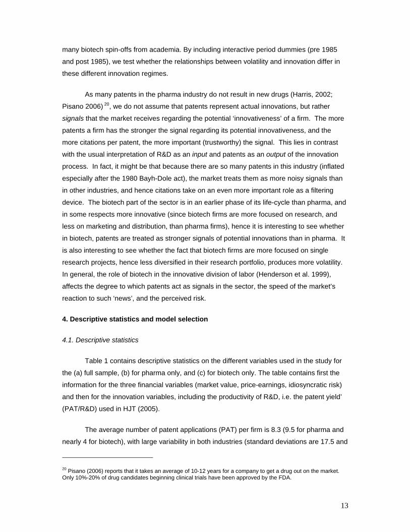
As many patents in the pharma industry do not result in new drugs (Harris, 2002;

Pisano 2006) 20, we do not assume that patents represent actual innovations, but rather

signals that the market receives regarding the potential ‘innovativeness’ of a firm. The more

patents a firm has the stronger the signal regarding its potential innovativeness, and the

more citations per patent, the more important (trustworthy) the signal. This lies in contrast

with the usual interpretation of R&D as an input and patents as an output of the innovation

process. In fact, it might be that because there are so many patents in this industry (inflated

especially after the 1980 Bayh-Dole act), the market treats them as more noisy signals than

in other industries, and hence citations take on an even more important role as a filtering

device. The biotech part of the sector is in an earlier phase of its life-cycle than pharma, and

in some respects more innovative (since biotech firms are more focused on research, and

less on marketing and distribution, than pharma firms), hence it is interesting to see whether

in biotech, patents are treated as stronger signals of potential innovations than in pharma. It

is also interesting to see whether the fact that biotech firms are more focused on single

research projects, hence less diversified in their research portfolio, produces more volatility.

In general, the role of biotech in the innovative division of labor (Henderson et al. 1999),

affects the degree to which patents act as signals in the sector, the speed of the market’s

reaction to such ‘news’, and the perceived risk.

4. Descriptive statistics and model selection

4.1. Descriptive statistics

Table 1 contains descriptive statistics on the different variables used in the study for

the (a) full sample, (b) for pharma only, and (c) for biotech only. The table contains first the

information for the three financial variables (market value, price-earnings, idiosyncratic risk)

and then for the innovation variables, including the productivity of R&D, i.e. the patent yield’

(PAT/R&D) used in HJT (2005).

The average number of patent applications (PAT) per firm is 8.3 (9.5 for pharma and

nearly 4 for biotech), with large variability in both industries (standard deviations are 17.5 and

20 Pisano (2006) reports that it takes an average of 10-12 years for a company to get a drug out on the market. Only 10%-20% of drug candidates beginning clinical trials have been approved by the FDA.

14

18.4 respectively). Employing a standardized measure of variability (coefficient of variation),

we observe that patenting activity is more heterogeneous amongst the biotech firms than the

pharma firms. In the case of weighted patents (PATW), both the sample mean and the

standard deviation are much higher for the biotech industry—indicating that although there

are more patents in pharma, they are on average more ‘important’ in biotech. Sample

means and standard deviations of R&D intensity are much higher in pharma than biotech

(though as is well known, what is counted as R&D in pharma, sometimes also includes

marketing type activities). The skewness measure indicates a high degree of asymmetry

(long right tails) for all the innovation variables, with R&D more skewed in pharma than

biotech, but patenting more skewed in biotech than pharma. The Kurtosis measure indicates

that the distributions (in both samples) are also leptokurtic compared to the normal.

With regards to the financial variables, the level of market value and the level of price

earnings (MKTVAL and P/E) exhibit a large amount of variation, while idiosyncratic risk (IR)

appears more concentrated around a normal distribution. They result all positively skewed

and leptokurtic, with the distribution of IR being closer to the normal. The average P/E for

biotech is three times that in pharma, as would be expected given the smaller average size

of biotech firms, the fact that they often have low earnings (Pisano 2006), and their higher

innovativeness (evidenced by their higher patent yield) hence higher expected growth.

Static correlations between the variables don’t show much significance, since, as will

be seen below, the variables are significant in the various regressions with different lags:

patents at time t are correlated with R&D intensity at time t-3. We do not perform lagged

correlations, if we view the correlations dynamically by plotting variables together over time,

we see some interesting relationships. From Figure 2a and 2b, idiosyncratic risk appears

remarkably correlated with both R&D intensity and, to a lesser extent in the biotech industry,

to citation weighted patents. These figures provide a first, albeit simplistic, indication of the

co-evolution of idiosyncratic risk and innovation—investigated more rigourously below.

It is interesting to see that in Figure 3 the rise in citation weighted patents is

accompanied in both pharma and biotech (but more so for biotech) by a rise in market share

instability21. This is precisely what would be expected by the literature on ‘competence-

destroying’ innovations (Tushman and Anderson 1986) and gives us a preliminary reason to

expect that citation weighted patents also affect the volatility of stock prices (as these are

21 The market share instability index is defined in Hymer and Pashigian (1962): |][| 1,

1−

=

−= ∑ ti

n

iit ssI , where

s=market share of firm i, and n=number of firms.

15

affected by the expected future market share of a firm). This result in fact confirms that

found in Mazzucato (2002): market share instability is highest in periods of the industry life-

cycle when innovation is the most ‘radical’ or competence destroying (discussed in 2.3).

4.2 Model selection

In the remaining sections, we test the relationship between the innovation variables

discussed above and the level and volatility of stock returns (all the variables in logs). We

first try to replicate the results found in HJT (2005) regarding the relationship between market

value, R&D, and patents. Second, we regress idiosyncratic risk on the innovation variables to

test whether firm specific risk is related to innovation, as hypothesized (but not tested) in

Campbell et al. (2001). Third we test the relationship between innovation and the level and

volatility of stock prices found in the “rational bubble” hypothesis (Pastor and Veronesi,

2004), by regressing the P/E ratio on idiosyncratic risk (IR) and then directly on the

innovation variables.

Specifically, the equations we test are:

Model 1

1a. ( ) tiLti

Ltiiti REV

RDMKTVAL ,

,

,, loglog εβα +⎟

⎟⎠

⎞⎜⎜⎝

⎛+=

−

−

1b. ( ) tiLtiLti

Ltiiti PAT

REVRD

MKTVAL ,,,

,, )(loglog εθβα ++⎟

⎟⎠

⎞⎜⎜⎝

⎛+= −

−

−

1c. ( ) ( ) tiLtiLti

Ltiiti PATW

REVRD

MKTVAL ,,,

,, logloglog εγβα ++⎟

⎟⎠

⎞⎜⎜⎝

⎛+= −

−

−

Model 2

2a. ( ) tiLti

Ltiiti REV

RDIDRISK ,

,

,, loglog εβα +⎟

⎟⎠

⎞⎜⎜⎝

⎛+=

−

−

2b. ( ) tiLtiLti

Ltiiti PAT

REVRD

IDRISK ,,,

,, )(loglog εθβα ++⎟

⎟⎠

⎞⎜⎜⎝

⎛+= −

−

−

2c. ( ) ( ) tiLtiLti

Ltiiti PATW

REVRD

IDRISK ,,,

,, logloglog εγβα ++⎟

⎟⎠

⎞⎜⎜⎝

⎛+= −

−

−

Model 3 3. ( ) ( ) tiLtiiti IDRISKEP ,,, log/log εϕα ++= −

16

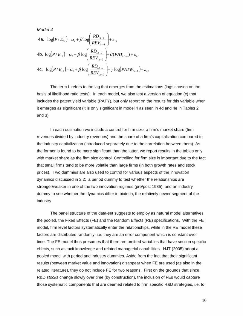
Model 4

4a. ( ) tiLti

Ltiiti REV

RDEP ,

,

,, log/log εβα +⎟

⎟⎠

⎞⎜⎜⎝

⎛+=

−

−

4b. ( ) tiLtiLti

Ltiiti PAT

REVRD

EP ,,,

,, )(log/log εθβα ++⎟

⎟⎠

⎞⎜⎜⎝

⎛+= −

−

−

4c. ( ) ( ) tiLtiLti

Ltiiti PATW

REVRD

EP ,,,

,, loglog/log εγβα ++⎟

⎟⎠

⎞⎜⎜⎝

⎛+= −

−

−

The term L refers to the lag that emerges from the estimations (lags chosen on the

basis of likelihood ratio tests). In each model, we also test a version of equation (c) that

includes the patent yield variable (PATY), but only report on the results for this variable when

it emerges as significant (it is only significant in model 4 as seen in 4d and 4e in Tables 2

and 3).

In each estimation we include a control for firm size: a firm’s market share (firm

revenues divided by industry revenues) and the share of a firm’s capitalization compared to

the industry capitalization (introduced separately due to the correlation between them). As

the former is found to be more significant than the latter, we report results in the tables only

with market share as the firm size control. Controlling for firm size is important due to the fact

that small firms tend to be more volatile than large firms (in both growth rates and stock

prices). Two dummies are also used to control for various aspects of the innovation

dynamics discussed in 3.2: a period dummy to test whether the relationships are

stronger/weaker in one of the two innovation regimes (pre/post 1985); and an industry

dummy to see whether the dynamics differ in biotech, the relatively newer segment of the

industry.

The panel structure of the data-set suggests to employ as natural model alternatives

the pooled, the Fixed Effects (FE) and the Random Effects (RE) specifications. With the FE

model, firm level factors systematically enter the relationships, while in the RE model these

factors are distributed randomly, i.e. they are an error component which is constant over

time. The FE model thus presumes that there are omitted variables that have section specific

effects, such as tacit knowledge and related managerial capabilities. HJT (2005) adopt a

pooled model with period and industry dummies. Aside from the fact that their significant

results (between market value and innovation) disappear when FE are used (as also in the

related literature), they do not include FE for two reasons. First on the grounds that since

R&D stocks change slowly over time (by construction), the inclusion of FEs would capture

those systematic components that are deemed related to firm specific R&D strategies, i.e. to

17

the independent variable. Second on the grounds that since firms change their strategies

over time in response to market signals, the FE model is inappropriate as it presumes

permanent firm specific effects.

In our case, the first point is irrelevant since we are dealing with volatile flow data and

not with slowly-changing stocks, hence FE are not likely to be excessively correlated with the

independent variable and thus to capture the sample correlation between the dependent and

independent variables. Concerning the second point, we believe that even if firm strategies

vary in response to time-varying market signals, the presence of publicly available

information on fundamentals may result in systematic cross-sectional factors, reflecting

relatively permanent aspects of the specific firm’s fundamentals that are not explicitly taken

into account in the model specification22.

For these reasons, unlike HJT (2005), we do not impose any particular model

specification and base our choices on statistical information only. The model selection

procedure is implemented in two steps, first evaluating the statistical relevance of the

individual (firm) effects and then whether they are correlated with the regressors. This is done

by testing, via the Breusch-Pagan LM test, for the presence of individual effects against the

common constant model (pooled estimator), and then testing the null of orthogonality of the

individual effects, i.e. the RE specification, assuming an FE as alternative hypothesis. In this

second step the reference evaluation tool is the Hausman test 23.

The Breusch-Pagan test rejects the null hypothesis of the pooled model (common

constant) for the entire set of specifications, suggesting to employ as a first step the RE

specification. After the Hausman test, an RE model is selected only for model 4. In all the

other cases a FE specification is selected. The model selection results are presented in

column 2 of Tables 2-3. At the current stage, we are still working on the biotech sample,

hence present here the results only for the whole sample and pharma.

22 We don’t think there is an objective reason to believe that firm specific effects are fixed over time and randomly distributed over the sample, as implied in the RE specification. Moreover, the RE model presumes that the section specific effects and the explanatory variables are uncorrelated. This assumption is questionable, since it is likely that the omitted factors that are relevant for the dependent variable are also relevant in determining the explanatory variable (Mundlack, 1978). As regards our specific analysis, the omitted factors no doubt include tacit knowledge and managerial capabilities, factors that have relevant effects on both innovative activity and the market performance of a given firm. 23 The Breusch-Pagan (1980) LM statistic tests whether the variance of individual effects in the error term is zero, hence it actually maintains the RE model under the null hypothesis.

18

5. Results

The results of the preferred models are summarized in Table 2 for the whole sample

and Table 3 for the pharma sample (biotech table available soon). When the estimations are

done using the FE estimator, introducing industry dummies (in the case of the whole sample)

does not make sense. Hence, with FE estimations we report the results without the

dummies. Yet when we look at the effect of this dummy in the first step of the Hausman test

when the RE estimator is used, we find that the sign and significance of the biotech dummy

is always significant, with a negative sign in model 1 (i.e. biotech firms have on average 10%

less market value than the sample mean), a positive sign in model 2 (biotech firms

experience on average 45% more idiosyncratic risk than the sample mean), and a positive

effect in models 3 and 4 (biotech firms have on average 30% higher P/E than the sample

mean).

Our estimates result substantially unchanged when employing the reduced sample

with end date fixed at 1995 in the place of 1999 (as done also in HJT 2005). This suggests

that our correction for the truncation problem, using the fixed effects methodology discussed

above, was efficient.

The inclusion of the post 1985 period dummy resulted statistically significant only for

model 2, signaling the possibility of a structural break in the dynamics of volatility after 1985.

However, as the inclusion of this dummy created some sample biases in the second period

(due also to the much larger number of firms in the second period, as is clear in Fig. 1), we

report the results without the dummy as it does not affect the results except to signal that

there is more firm specific volatility in the second period, a result confirmed in the work of

Campbell et al. (2001). We plan to study this phenomenon more in our future work, trying to

link it to changes in the search (innovation) regimes discussed in Gambardella (1995) and

elsewhere.

Column 5 in Tables 3 and 4 shows that the sign for the control of firm size (market

share) is as expected: firm size has a positive effect on the level of market value, but a

negative effect on volatility and the price-earnings ratio. That small firms experience more

volatility, in both growth and stock prices, is a well known phenomenon. The fact that small

firms also have high price-earnings is easier to interpret for highly innovative firms who have

low earnings but high potential growth. It is less easy to interpret for those small firms that

are not particularly innovative, but we cannot look into this unless we put their innovativeness

as the dependent variable (something we may explore in our future work). The use of the

firm’s capitalization share as the control for firm size instead results statistically insignificant

19

when employing the FE estimator, signaling that this effect is relatively stable over time and

captured by the firm specific dummies (even if significant in the RE regressions, its presence

does not alter the qualitative and quantitative results of the estimates).

In what follows we review the results from Models 1-4, commenting only on the effect

that the various innovation variables have on market share, idiosyncratic risk and price-

earnings (note: as in this version of the paper we are still in the process of analyzing the

separate biotech sample, we focus our comments mainly on the whole and pharma

samples).

Model 1: Market value and innovation

Results for model 1 illustrate that R&D intensity, patent counts, and weighted patents

have a positive and significant effect (each at the 1% level) on the level of market value. It is

interesting that positive results arise even when using flow data, instead of the usual stock

measures used in the market value and innovation literature (HJT 2005). Furthermore, the

introduction of the simple patent count does not lead to a statistically insignificant R&D

intensity coefficient, as it does when using stock measures.

When the patent count variable is entered in 1b, the R&D intensity coefficient is

reduced in size, signaling that there is a certain degree of correlation between R&D intensity

lagged 2 years and current patent applications. When we run the pharma and biotech

samples separately, the reduction in the size of the coefficient is stronger in the biotech

industry, signaling the presence of a higher correlation between PAT and R&D intensity in

this part of the industry (not surprising given the higher mean patent yield in biotech). This

result is consistent with a mean patent application lag respect to R&D expenditure of

approximately 3 years24.

In each of the equations in model 1, R&D is most significant with a lag of 2 years, and

patents with no lags. This suggests that the market reacts quicker to news on patents than

to news on R&D, most probably due to its understanding of the lengthy process of research

in this industry (Pisano 2006).

When patents are weighted by citations received (1c) the estimated coefficients are

bigger in size and their statistical significance strongly improved, irrespective of the specific

sample being considered. When employing patents weighted by citations made, rather than

received, the R&D intensity coefficient resulted weaker in both size and statistical terms. In

24 The regression of patent applications on R&D intensity results statistically significant, and the best fit is obtained when the explanatory variable is entered with three lags.

20

sum, the equation fit is consistent with the result of HJT [2005], and improves strongly when

patents are weighted by citations received (as in HJT 2005). The introduction of the patent

yield variable proved insignificant, and as it is correlated with our measures of patents and

R&D we did not include it in the tables (unless significant).

Model 2: Idiosyncratic risk and innovation

In model 2 we evaluate the hypothesis that idiosyncratic risk is related to firm level

innovation, as proxied by R&D intensity, patents and weighted patents. We find that the

innovation variables are significant, but less so here than in model 1. R&D intensity is always

significant, with its significance increasing from 10% to 5% when patent measures are

included as well. Although patent counts are not significant, weighted patents are (at the

10% level). Thus unlike market value in model 1, it appears that volatility reacts more

strongly to citation weighted patents (i.e. more important patents) than simple patent counts.

As in model 1 the lag on R&D is higher than that on patents (2 and 1 years

respectively), yet patents have a higher lag in model 2 than in model 1. The lags we find

seem reasonable as they suggest that R&D investment takes time to have an effect on

volatility, while patents don’t. It might also be that the market foresees the patent application

given the spending on R&D that has already occurred. As in model 1, patent yield is

insignificant.

When we ran the pharma and biotech samples separately, we found that in the case

of pharma the significance of patents and weighted patents rose significantly (to the 5%

level), while patent yield remained insignificant. The lags in pharma are higher than those in

the combined sample, suggesting that the market takes longer to react to older segments of

the sector (a hypothesis we are currently investigating further).

Model 3: Price-earnings ratios and idiosyncratic risk (rational bubble)

Pastor and Veronesi (2004) claim that if one includes the uncertainty about a firm’s

average future profitability into market valuation models, then bubbles can be understood as

emerging from rational behavior about expected future profitability25. As discussed above,

this model predicts a positive relationship between the level and volatility of stock returns,

25 Pastor and Veronesi (2004) use the Market to Book ratio (M/B), which replaces the P/D ratio employed in the theoretical derivations of Gordon’s growth formula, on the grounds that dividends are not paid out by small start ups. We instead use P/E instead of P/D since both earnings and dividends, are proxies for the “fundamental” value underlying stock movements.

21

both increasing when new technologies first emerge, then falling when the uncertainty

around the technologies decreases. With models 3 and 4 we evaluate these hypotheses

empirically: we first regress price-earnings on idiosyncratic risk (model 3), and then price-

earnings on the various innovation measures (model 4).

In model 3 we obtain a positive and statistically significant coefficient for idiosyncratic

risk, at the 1% level in the whole sample as well as the separate samples. The best

estimates are obtained when IR is entered with 0 lags, suggesting a simultaneous

relationship between the level of P/E and the volatility of returns, as would in fact be

predicted by the rational bubble hypothesis. This significant relationship between the level of

price-earnings and the volatility of firm specific returns, also finds support in the empirical

literature on the high frequency relationship between prices (or returns) and market

volatility26.

Model 4 Price earnings and innovation

Finally, we regress P/E on the various innovation variables used above. As discussed

previously, this is the only model that is estimated using random effects. As in model 1, R&D

is significant at the 1% level, but unlike model 1, the patent count variable is negative (and

significant). Weighted patents are positive and significant at the 5% level. Unlike the previous

models, patent yield is also significant (at the 5% level), in both the combined and pharma

sample, suggesting that, amongst the financial variables, P/E best reflects the potential

innovativeness of a firm as it is more related to the ‘efficiency’ of innovation expenditures

than the other financial variables. The lag structure is the same as in the models above, also

in the separate samples.

As already discussed, the biotech dummy is positive and significant, indicating that on

average biotech firms have a P/E ratio 30% higher than the sample mean. This is to be

expected given that small innovative biotech firms often have low earnings, so that their

stock valuation is determined largely by their investment in innovation (note the higher mean

P/E for biotech firms in Table 1).

This positive relationship between P/E and innovation provides support to the rational

bubble model in Pastor and Veronesi (2004; 2005) where it is assumed, but not proved, that

P/E should be higher for firms that introduce radical technologies.

26 The rationale is that increasing portfolio risk is compensated by augmented expected returns. The ARCH-in mean specification in GARCH modeling for financial time series aims at directly accounting for this relationship.

22

6. Conclusion

Our study provides empirical support to the untested assumption in recent finance

literature that the volatility of stock prices (both aggregate and idiosyncratic) is related to

innovation. We use firm level R&D and patent data (citation weighted) to test whether firms

that are ‘more innovative’ are characterized by higher volatility of stock returns, compared to

those in the general market, and higher relative levels of market value and P/E.

The lag structure of the innovation variables (in each of the models) provides insights

into the speed at which the market reacts to innovation ‘signals’. Lags are higher for R&D

than for patents, suggesting that the market reacts more quickly to signals regarding

innovation outputs than inputs. It is sensible to think that uncertainty is in fact highest at the

time a patent is applied for, since this includes the uncertainty regarding whether the patent

will be granted, as well as uncertainty regarding the effect of the patent on the firm’s growth.

This is especially true in the pharma sector where there is a high patenting rate but a very

low rate of new drug discovery (Orsenigo, Dosi and Mazzucato 2006). Pisano (2006), in fact,

claims that one way that the pharma and biotech industries differs from other high tech

industries, such as computers and software, is the profound and persistent uncertainty of the

R&D process due to the limited knowledge of human biological systems (as opposed to

chemical or electronic)27. The fact that in all the models weighted patents are more

significant than patent counts, suggests that the market is relatively efficient in understanding

which patents are more important, and to not be fooled by the patent inflation that has

occurred especially since the 80’s.

We find that volatility is higher in the case of small firms (proxied by market share)

and in the post 1985 period, characterized by a more guided search regime (due to scientific

and organizational changes described in Gambardella 1995). The higher volatility in the

latter period is most likely related to the fact that this period is characterized by an ‘inflation’

of patents (due to the effect of the 1980 Bayh-Dole act on patenting behavior), which reduces

their reliability as a ‘signal’ of real innovation (hence more mistakes made by investors).

Though the fact that weighted patents have a stronger effect on volatility (as well as P/E)

than simple patent counts, suggests that the market is able to, at least partially, filter through

this noise.

Finally, we reproduce the results found in the market value and innovation literature

(HJT 2005) using flow rather than stock variables, and also find a positive relationship

27 This is one of the reasons for its low R&D productivity, a delusion for those that hoped that biotech’s more nimble structure would save pharma’s low turnout of new drugs.

23

between the P/E ratio and the innovation variables, as would be predicted by the ‘rational

bubble’ hypothesis (as well as a direct relationship between P/E and idiosyncratic risk).

Interestingly, it is especially the P/E ratio that reflects the efficiency of the innovative process

(the patent ‘yield’). This supports the view that price-earnings are guided by expected future

profitability of highly innovative firms. The fact that most biotech companies have no earnings

(exceptions are the very big ones like Amgen and Genentech), means in fact that their value

is determined almost exclusively by their ongoing innovation projects. Yet the fact that the

R&D process is so lengthy and the projects so uncertain, means that valuation of firms is full

of mistakes. The corrections that emerge from this trial and error process are no doubt partly

responsible for the stock return volatility associated with the various innovation variables.

In our future work we plan to take more into consideration the rich source of

information provided in patent citation data. For example, is volatility higher for firms that

have more ‘original’, as opposed to more ‘general’, patents (see footnote 7)? We plan to also

pay more attention to the temporal dimension of citations by asking whether recent citations

have more effect on volatility.

References

Campbell, J.Y., Lettau, M., Malkiel, B.G., and Yexiao, X. (2001). “Have Individual Stocks Become More Volatile? An Empirical Exploration of Idiosyncratic Risk,” Journal of Finance, 56: 1-43. Compustat Database (2001). New York: Standard and Poor’s Corporation. Davis, S.J. and Haltiwanger, J. (1992). “Gross Job Creation, Gross Job Destruction , and Employment Reallocation,” Quarterly Journal of Economics, 107: 819-64. Deng, Y. (2005). “The Value of Knowledge Spillovers,” Paper presented at the CEF annual conference, Washington DC, June 24, 2005. Filson, D. (2001). “The Nature and Effects of Technological Change over the Industry Life Cycle,” Review of Economic Dynamics, 4(2): 460-94. Gambardella (1995). Science and Innovation: The US Pharmaceutical Industry During the 1980s, Cambridge University Press, Cambridge, UK. Gort, M. and Klepper, S. (1982). “Time Paths in the Diffusion of Product Innovations,” Economic Journal, 92: 630-653. Greenwood, J. and Jovanovic, B. (1999). “The IT Revolution and the Stock Market,” American Economic Review, 89(2): 116-122. Griliches, Z., Hall. B., and Pakes, A. (1991). R&D, Patents and Market Value Revisited: Is There ad Second (Technological Opportunity) Factor?,” Economics, Innovation and New Technology, Vol. 1: 1983-201.

24

Hall, B., A. Jaffe, and M. Trajtenberg (2001b). “The NBER Patent Citations Data File,” in Jaffe, A.B. and Trajtenberg, M. (2002), Patents, Citations and Innovations: a Window on the Knowledge Economy, MIT Press, Boston, MA. Hall, B., A. Jaffe, and M. Trajtenberg (2005). “Market value and patent citations,” Rand Journal of Economics, Vol. 36(5) Harris, G. (2002). “Why drug makers are failing in quest for new blockbusters,” Wall Street Journal, March 18, 2002. Henderson, R., Orsenigo, L. and Pisano, G. (1999). “The Pharmaceutical Industry and the Revolution in Molecular Biology: Interactions among Scientific, Institutional and Organizational change”, in Mowery, D. and Nelson, R. (eds.), Sources of Industrial Leadership, Cambridge, 1999. Jaffe, A.B. and Trajtenberg, M. (2002). Patents, Citations and Innovations: a Window on the Knowledge Economy, MIT Press, Boston, MA. Jovanovic, B. (1982). “Selection and the Evolution of Industry,” Econometrica, 50 (3), 649-70. Jovanovic, B., and MacDonald, G.M. (1994). “The Life Cycle of a Competitive Industry,” Journal of Political Economy, 102 (2): 322-347. Klepper, S. (1996). “Exit, Entry, Growth, and Innovation over the Product Life-Cycle,” American Economic Review, 86(3): 562-583. Knight, F.H. (1921). Risk, Uncertainty and Profit, Boston: Houghton Mifflin. Mazzucato, M., and Semmler, W. (1999). “Stock Market Volatility and Market Share Instability during the US Auto industry Life-Cycle,” Journal of Evolutionary Economics, 9 (1): 67-96. Mazzucato, M. (2002). “The PC Industry: New Economy or Early Life-Cycle,” Review of Economic Dynamics, 5: pp. 318-345. Mazzucato, M. (2003). “Risk, Variety and Volatility: Innovation, Growth and Stock Prices in Old and New Industries,” Journal of Evolutionary Economics, Vol. 13 (5), 2003: pp. 491-512. Mazzucato, M. and Tancioni, M. (2005). “Idiosyncratic Risk and Innovation,” Open University Discussion Paper 2005-50. Mazzucato and Tancioni (2006). ”Indices that Capture Creative Destruction: Questions and Implications,” Revue d’Economie Industrielle. 110, 2nd trimester: 199-218. Mundlack, Y. (1978). “On the Pooling of Time Series and Cross Section Data”,Econometrica, Vol 46, pp 69-85. Marsili, O. (2001). “The Anatomy and Evolution of Industries”, Northampton, MA, Edward Elgar.

Orsenigo, L. Pammolli, F. Riccaboni, M. (2001), “Technological change and network dynamics. Lessons from the pharmaceutical industry.” Research Policy, 30: 485-509. Pakes, A. (1985). “On Patents, R&D, and the Stock Market Rate of Return,” Journal of Political Economy, Vol. 93(2): 390-409.

25

Pastor, L. and Veronesi, P. (2004). “Was There a Nasdaq Bubble in the Late 1990’s,” Journal of Financial Economics, 81 (1): 61-100. Pastor, L. and Veronesi, P. (2005). “Technological Revolutions and Stock Prices,” National Bureau of Economic Research w11876. Pavitt, K. (1984). “Sectoral Patterns of Technical Change: Towards a Taxonomy and a Theory,” Research Policy, Vol. 13: 342-373. Pisano, G. (2006). “Can Science Be a Business?,” Harvard Business Review, October 2006: 1-12. Schwert, G.W. (1989). “Why Does Stock Market Volatility Change Over Time? Journal of Finance, 54: 1115-1153. Schwert, G.W. (2002). “Stock Market Volatility in the New Millenium: How Wacky is Nasdaq?”, Journal of Monetary Economics, 49: 3-26. Shiller, R.J. (1981). “Do Stock Prices Move Too Much to be Justified by Subsequent Changes in Dividends,” American Economic Review, 71: 421-435. Shiller, R.J. (2000). Irrational Exuberance Princeton University Press, Princeton. Trajtenberg, M. (1990). “A Penny for Your Quotes: Patent Citations and the Value of Innovations,” Rand Journal of Economics, 21 (1): 172-187. Tushman, M., and Anderson, P. (1986). “Technological Discontinuities and Organizational Environments,” Administrative Science Quarterly, 31: 439-465. U.S. Department of Commerce. Bureaus of Economic Analysis. “Computer Prices in the National Accounts: An Update from the Comprehensive Revision.” Washington, D.C., June 1996.

26

Figure 1

Number of Firms (1962-1999)

0

20

40

60

80

100

120

140

1962

1964

1966

1968

1970

1972

1974

1976

1978

1980

1982

1984

1986

1988

1990

1992

1994

1996

1998

Years

Com

bine

d N

umbe

r of F

irms

Pharmaceutical

Biotechnology

27

Figure 2 Dynamic correlations

Pharma Biotech

100.0150.0200.0250.0300.0350.0400.0450.0500.0550.0600.0

1962

1966

1970

1974

1978

1982

1986

1990

1994

1998

2002

0.0%

10.0%

20.0%

30.0%

40.0%

50.0%

60.0%

IR (1962 = 100) R&D/Revenues

0.00

100.00

200.00

300.00

400.00

500.00

600.00

700.00

800.00

1979

1982

1985

1988

1991

1994

1997

2000

2003

0.0%5.0%10.0%15.0%20.0%25.0%30.0%35.0%40.0%45.0%50.0%

IR (1980 = 100) R&D/Revenues

2a) Idiosyncratic risk (IR) and R&D intensity

100.0150.0200.0250.0300.0350.0400.0450.0500.0550.0600.0

1962

1966

1970

1974

1978

1982

1986

1990

1994

1998

2002

0.00

0.50

1.00

1.50

2.00

2.50

3.00

IR (1962 = 100) PATW

0.00

100.00

200.00

300.00

400.00

500.00

600.00

700.00

800.00

1979

1982

1985

1988

1991

1994

1997

2000

0.0

0.5

1.0

1.5

2.0

2.5

3.0

3.5

4.0

IR (1980 = 100) PATW

2b) Idiosyncratic risk (IR) and weighted patents (corrected for truncation)

28

Figure 3 Innovation and market share instability

3a

Pharma: Market Share Instability vs PATW

0

500

1000

1500

2000

2500

3000

3500

4000

1962

1964

1966

1968

1970

1972

1974

1976

1978

1980

1982

1984

1986

1988

1990

1992

1994

Year

Pate

nt N

umbe

r

0

5

10

15

20

25

30

35

40

45

50

Inst

abili

ty In

dex

Wght PatentsIndustry Instability Index

3b

Biotech: Market Share Instability Index vs. PATW

0

200

400

600

800

1000

1200

1400

1600

1962

1964

1966

1968

1970

1972

1974

1976

1978

1980

1982

1984

1986

1988

1990

1992

1994

Year

Pate

nt N

umbe

r

0

5

10

15

20

25

30

35

40

45

Inst

abili

ty In

dex

Wght PatentsIndustry Instability Index

j

29

Table 1 Descriptive statistics

WHOLE MKTVAL PE IR_SP500 IR_IND RD/REV PAT PATW PATYIELD

Mean 5917.147 86.381 0.088 0.085 0.094 8.309 1.457 0.124 Median 787.646 25.408 0.071 0.071 0.054 1.000 0.058 0.001 Maximum 171234.700 9926.505 0.779 2.222 8.413 155.000 69.818 12.870 Minimum 1.697 0.423 -0.029 -0.266 0.000 0.000 0.000 0.000 Std. Dev. 17573.270 427.242 0.072 0.112 0.327 17.527 4.201 0.566 Skewness 5.328 16.312 2.685 9.574 18.844 3.325 9.132 14.757 Kurtosis 35.938 324.173 17.848 167.215 434.910 16.536 121.885 288.691

PHARMA MKTVAL PE IR_SP500 IR_IND RD/REV PAT PATW PATYIELD

Mean 7166.306 43.123 0.077 0.081 0.119 9.530 1.237 0.091 Median 998.557 22.768 0.063 0.068 0.078 1.000 0.105 0.003 Maximum 171234.700 4108.527 0.420 0.420 8.413 118.000 22.000 3.890 Minimum 1.697 4.357 -0.029 -0.083 0.000 0.000 0.000 0.000 Std. Dev. 19589.670 158.310 0.058 0.061 0.366 18.407 2.598 0.288 Skewness 4.724 21.204 1.503 1.135 17.009 2.772 3.846 6.548 Kurtosis 28.515 531.733 6.691 6.210 350.434 11.392 21.954 59.816

BIOTECH MKTVAL PE IR_SP500 IR_IND RD/REV PAT PATW PATYIELD

Mean 1422.355 242.034 0.126 0.101 0.004 3.913 2.252 0.240 Median 234.938 56.036 0.105 0.082 0.002 0.000 0.000 0.000 Maximum 39131.630 9926.505 0.779 2.222 0.066 155.000 69.818 12.870 Minimum 3.731 0.423 -0.027 -0.266 0.000 0.000 0.000 0.000 Std. Dev. 3708.635 848.918 0.100 0.209 0.006 13.023 7.499 1.077 Skewness 6.007 8.576 2.778 6.393 5.693 8.181 6.559 9.124 Kurtosis 52.096 87.553 14.786 60.349 52.081 85.894 51.626 96.567

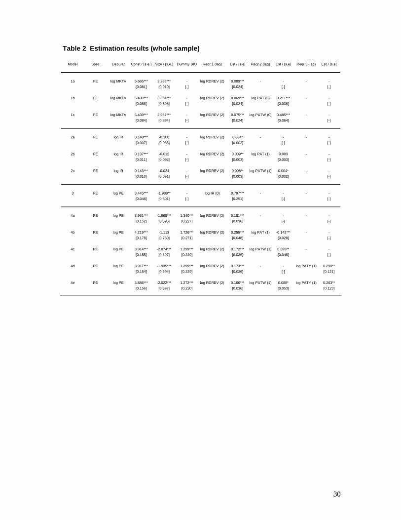
30

Table 2 Estimation results (whole sample)

Model Spec Dep var Const / [s.e.] Size / [s.e.] Dummy BIO Regr.1 (lag) Est / [s.e] Regr.2 (lag) Est / [s.e] Regr.3 (lag) Est / [s.e]

1a FE log MKTV 5.665*** 3.285*** - log RDREV (2) 0.089*** - - - -[0.081] [0.910] [-] [0.024] [-] [-]

1b FE log MKTV 5.400*** 3.354*** - log RDREV (2) 0.069*** log PAT (0) 0.211*** - -[0.088] [0.898] [-] [0.024] [0.036] [-]

1c FE log MKTV 5.439*** 2.957*** - log RDREV (2) 0.075*** log PATW (0) 0.485*** - -[0.084] [0.894] [-] [0.024] [0.064] [-]

2a FE log IR 0.148*** -0.100 - log RDREV (2) 0.004* - - - -[0.007] [0.086] [-] [0.002] [-] [-]

2b FE log IR 0.137*** -0.012 - log RDREV (2) 0.009** log PAT (1) 0.003 - -[0.011] [0.092] [-] [0.003] [0.003] [-]

2c FE log IR 0.143*** -0.024 - log RDREV (2) 0.008** log PATW (1) 0.004* - -[0.010] [0.091] [-] [0.003] [0.002] [-]

3 FE log PE 3.445*** -1.988** - log IR (0) 0.797*** - - - -[0.048] [0.801] [-] [0.251] [-] [-]

4a RE log PE 3.961*** -1.965*** 1.340*** log RDREV (2) 0.181*** - - - -[0.152] [0.695] [0.227] [0.036] [-] [-]

4b RE log PE 4.219*** -1.113 1.726*** log RDREV (2) 0.255*** log PAT (1) -0.142*** - -[0.178] [0.760] [0.271] [0.048] [0.028] [-]

4c RE log PE 3.914*** -2.074*** 1.299*** log RDREV (2) 0.172*** log PATW (1) 0.099** - -[0.155] [0.697] [0.229] [0.036] [0.048] [-]

4d RE log PE 3.917*** -1.935*** 1.299*** log RDREV (2) 0.173*** - - log PATY (1) 0.290**[0.154] [0.694] [0.229] [0.036] [-] [0.121]

4e RE log PE 3.886*** -2.022*** 1.272*** log RDREV (2) 0.166*** log PATW (1) 0.088* log PATY (1) 0.263**[0.156] [0.697] [0.230] [0.036] [0.053] [0.123]

31

Table 3 Estimation results (pharma sample)

Model Spec Dep var Const / [s.e.] Contr / [s.e.] Dummy 85 Regr.1 (lag) Est / [s.e] Regr.2 (lag) Est / [s.e] Regr.3 (lag) Est / [s.e]

1a FE log MKTV 4.829*** 6.065*** 1.996*** log RDREV (3) 0.152** - - - -[0.078] [1.589] [0.070] [0.069] [-] [-]

1b FE log MKTV 4.513*** 8.009*** 1.753*** log RDREV (3) 0.140** log PAT (2) 0.370*** - -[0.081] [1.526] [0.071] [0.066] [0.038] [-]

1c FE log MKTV 4.661*** 6.770*** 1.804*** log RDREV (3) 0.144** log PATW (2) 0.652*** - -[0.079] [1.546] [0.073] [0.067] [0.086] [-]

2a FE log IR 0.090*** -0.038 0.011** log RDREV (1) 0.021*** - - - -[0.003] [0.082] [0.004] [0.003] [-] [-]

2b FE log IR 0.088*** -0.010 0.009** log RDREV (1) 0.008* log PAT (1) 0.004** - -[0.004] [0.083] [0.004] [0.004] [0.002] [-]

2c FE log IR 0.089*** -0.023 0.009** log RDREV (1) 0.008* log PATW (1) 0.010** - -[0.004] [0.082] [0.004] [0.004] [0.005] [-]

3 FE log PE 3.091*** 0.140 0.116** log IR (1) 0.889** - - - -[0.063] [0.956] [0.050] [0.412] [-] [-]

4a RE log PE 3.248*** -0.906 0.139*** log RDREV (2) 0.566*** - - - -[0.102] [1.001] [0.050] [0.190] [-] [-]

4b RE log PE 3.290*** -0.916 0.208*** log RDREV (2) 0.570*** log PAT (2) -0.103*** - -[0.103] [0.995] [0.053] [0.190] [0.026] [-]

4c RE log PE 3.280*** -1.026 0.118** log RDREV (2) 0.642*** log PATW (1) 0.107** - -[0.093] [1.008] [0.054] [0.184] [0.056] [-]

4d RE log PE 3.191*** -0.761 0.139*** log RDREV (2) 0.599*** - - log PATY (1) 0.486***[0.102] [0.993] [0.049] [0.188] [-] [0.146]

4e RE log PE 3.244*** -0.872 0.131*** log RDREV (2) 0.661*** log PATW (1) 0.097* log PATY (1) 0.476***[0.094] [1.005] [0.053] [0.184] [0.056] [0.162]