Stochastic weather generators with non-homogeneous …pagesperso.univ-brest.fr/~ailliot/SlidesAber/Monbet_Aber.pdf · Stochastic weather generators with non-homogeneous hidden Markov

Stochastic weather generatorswith non-homogeneous hidden Markov switching

Application to temperature series

Valérie Monbet 1, Pierre Ailliot2

1IRMAR, Rennes 12LMBA, UBO

Monbet, Ailliot Switching autoregressive models

Stochastic weather generators?

Stochastic tools for generating sequences of meteorological variables

Historical data Stochastic model Synthetic data

40 years of daily meantemperature at Brest

SWGEN calibrated onhistorical data

Large number of synthetictemperature sequences withstatistical properties similar tooriginal data

→ ...


Stochastic weather generators?

Stochastic tools for generating sequences of meteorological variables

Used in impact studies when climate is involved and not enough data to estimate thequantities of interest

Synthetic weather conditions → System → Distribution of the response

Most usual applications: hydrology and agricultureMeteorological variables: rainfall, temperature, solar radiation, humidity, wind speed,...

In this talk, firstly focus on daily mean temperature at a single locationBrest, 40 years, ∆t = 1 dayPreprocessing step to remove seasonal components (+ trends, daily components)?In this talk, data blocked by month, results for January


Some existing stochastic weather generators

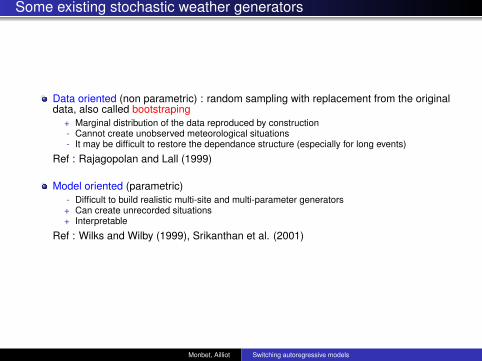
Data oriented (non parametric) : random sampling with replacement from the originaldata, also called bootstraping

+ Marginal distribution of the data reproduced by construction- Cannot create unobserved meteorological situations- It may be difficult to restore the dependance structure (especially for long events)

Ref : Rajagopolan and Lall (1999)

Model oriented (parametric)- Difficult to build realistic multi-site and multi-parameter generators+ Can create unrecorded situations+ Interpretable

Ref : Wilks and Wilby (1999), Srikanthan et al. (2001)


Transformed Gaussian processes

Classical approach for modeling time seriesSimulation of the stationary time series {Yt} in three steps:

First step: find a deterministic monotonic function g such that

Xt = g(Yt )

has (approximatively) Gaussian margins"Normal score transformation": g = Φ−1 ◦ FYFY (y) = P[Yt < y ], Φ cdf ofN (0, 1)

"Box-cox transformation": g(y) = yλ−1λ

Second step: {Xt} is a stationary process with (approximately) Gaussian margins. Furtherassume that {Xt} is a Gaussian process and simulate this process.

Exact simulationARMA models

Third step: apply the inverse transform g−1 to the simulated Gaussian sequence

Temperature dataTransformation to Gaussian margins : Y (transf )

t = g(Yt ) =√

13− Yt

Time series model AR(2) : Y transft = 0.57 + 0.83Y transf

t−1 − 0.07Y transft−2 + 0.41εt

Inverse transformation Yt = g−1(Y (transf )t ) = 13− (Y (transf )

t )2

Ref : Brockwell and Davies (2002), Monbet et al. (2007)



Temperatures are too hot: transformation?

Correlation function decreases too slow for short lags and is good for large lags:mixture of AR models?Transformed Gaussian process can not reproduce some non-linearities:

A stationary Gaussian process has a symmetric behavior below α and above 1− α quantileThe same holds true for transformed Gaussian processes (since g is monotonic)Observed hot regimes have shorter durations than cold regimes

data, simulation



+ Easy to implement

+ Can be used for multivariate data (several sites and/or variables)

- May be hard to interpret

- Can not reproduce some non-linearities

Alternatives?xxx - More general transformation Xt = g(Yh(t)) with g and h (stochastic?)xxxxx transformations such that {Xt} is a Gaussian processxxx - Non-linear time series models


Event-based models

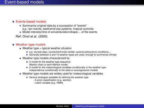
Events-based modelsSummarize original data by a succession of "events"e.g. rain events, swell/wind sea systems, tropical cyclonesModel intensity/time of arrival/duration/shape/... of the events

Ref: Onof et al. (2000)

Weather type modelsWeather type = typical weather situation

e.g. dry/wet days, convective/frontal rainfall, cyclonic/anticyclonic conditions,...Generally between 2 and 10 weather types are used; enough to summarize climate

Weather type models characterized byA model for the weather type sequenceMarkov chain or semi-Markov model.A model for the meteorological variables conditionally to the weather typeIndependence conditionally to the state or autoregressive models.

Weather type models are widely used for meteorological variablesVarious strategies available for defining the weather typexxx - A priori classification (e.g. wet/dry)xxx - Latent variable (e.g. HMM)


Weather type models

An example : the chain dependent model (Richardson, 1981)Weather type St ={Dry,Wet}

First order Markov chain with 2 states

Rainfall amount Rt conditionally independent in time given the weather type sequenceTemperature, solar radiation, wind speed Yt

Residual correlation between successive observations modeled as an AR process with time varyingcoefficients

Yt = β(St )

0 + β(St )

1 Yt−1 + σ(St )

εt

(β(s)i ), (σ(s)) unknown parameters and {εt} a Gaussian white noise

Rainfall · · · Rt−1 Rt Rt+1 · · ·↑ ↑ ↑

Weather type (wet/dry) · · · → St−1 → St → St+1 → · · ·↓ ↓ ↓

Temperature, ( wind, ...) · · · → Yt−1 → Yt → Yt+1 → · · ·

Temperature dynamics modeled as a mixture of two AR(2) processes


Richardson’s model for temperature time series

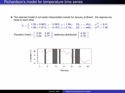
The selected model is not easily interpretable (results for January at Brest) : the regimes areclose to each other

Yt =

{1.26 + 0.88Yt−1 − 0.08Yt−2 + 1.96εt (St−1 = dry), µ(1) = 6.411.28 + 1.01Yt−1 − 0.18Yt−2 + 2.10εt (St−1 = wet), µ(2) = 7.39

Transition matrix :[

0.55 0.450.33 0.77

], stationary distribution

[0.240.76

]


Richardson’s model for temperature time series

Introduction of weather states gives more flexibility to the model→ marginal distribution better reproduced than in Box and Jenkins model→ idem for low level up crossings.

But, the dry/wet classification seems not convenient for the temperature for Brest’sclimate.

The non linearities are still not reproduced by the model.

Weather types can be obtained from other variables?


Clustering on meteorological variables (e.g. pressure,...)

Pressure, Wind, Rainfall · · · Rt−1 Rt Rt+1 · · ·↓ ↓ ↓

Weather type · · · → St−1 → St → St+1 → · · ·↓ ↓ ↓

Temperature · · · → Yt−1 → Yt → Yt+1 → · · ·

Pression Wind PrecipitationsRegime 1 (anticlyclonic) 1021 8.5 ms−1 1.04 mmRegime 2 (clyclonic) 1007 12.4 ms−1 11.79 mm

Model

Yt =

{1.42 + 0.73Yt−1 + 0.02Yt−2 + 1.90εt (St−1 = anticyclonic), µ(1) = 5.881.26 + 0.88Yt−1 − 0.08Yt−2 + 1.96εt (St−1 = cyclonic), µ(2) = 6.41

with non parametric semi-Markov transitions.



This classification is close to the wet/dry’s one?



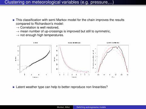
This classification with semi Markov model for the chain improves the resultscompared to Richardson’s model:→ Correlation is well restored,→ mean number of up-crossings is improved but still to symmetric,→ not enough high temperatures.

Latent weather type can help to better reproduce non linearities?


A SWGEN model for the temperature

Introduce the weather type as a latent (hidden) variable:"Markov Switching AutoRegressive" model (MS-AR)

Weather type (hidden) · · · → St−1 → St → St+1 → · · ·↓ ↓ ↓


+ Estimation procedure will find the "optimal" weather type- Estimation procedure more complicated, simpler models are needed

Hidden weather type modeled as a first order Markov chain

Linear Gaussian AR(p) model for the temperature evolution conditionally to theweather type

Yt = β(St )0 + β

(St )1 Yt−1 + ...β

(St )p Yt−p + σ(St )εt

(β(s)i ), (σ(s)) unknown parameters and {εt} iidN (0, 1) sequence

Maximum likelihood estimates (MLE) can be computed with the EM algorithm


A MS-AR model for the temperature

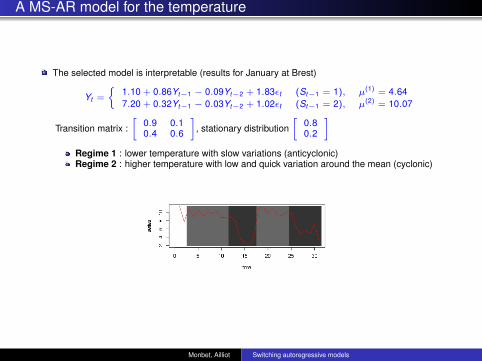
The selected model is interpretable (results for January at Brest)

Yt =

{1.10 + 0.86Yt−1 − 0.09Yt−2 + 1.83εt (St−1 = 1), µ(1) = 4.647.20 + 0.32Yt−1 − 0.03Yt−2 + 1.02εt (St−1 = 2), µ(2) = 10.07

Transition matrix :[

0.9 0.10.4 0.6

], stationary distribution

[0.80.2

]Regime 1 : lower temperature with slow variations (anticyclonic)Regime 2 : higher temperature with low and quick variation around the mean (cyclonic)



data, simulation

The model is able toreproduce some importantstatistical properties of thedata



MS-AR models much better reproduce the observed asymmetry in up-crossing rateNo enough variability around middle levels?

A priori classification MS-AR model

In MS-AR models the regime switchings are independent of past temperatureconditions

The probability of staying in the cold regime at time t is higher if the temperature is low attime t − 1?Adding this in the model could create more asymmetry?


A non-homogeneous MS-AR models for the temperature

Hidden Regime · · · → St−1 → St → St+1 → · · ·↓ ↗ ↓ ↗ ↓


Logistic link function for the switching probabilities. For s ∈ {1, 2},

P(St = s|St−1 = s,Yt−1 = yt−1) = π(s)− +

1− π(s)− − π

(s)+

1 + exp(λ

(s)0 + λ

(s)1 yt−1

)Linear Gaussian AR(p) model for the temperature conditionally to the weather type

Yt = β(St )0 + β

(St )1 Yt−1 + ...β

(St )p Yt−p + σ(St )εt

(β(s)i ), (σ(s)) unknown parameters and (εt ) iid sequence ofN (0, 1) r.v.


A non-homogeneous MS-AR models for the temperature

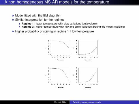
Model fitted with the EM algorithmSimilar interpretation for the regimes

Regime 1 : lower temperature with slow variations (anticyclonic)Regime 2 : higher temperature with low and quick variation around the mean (cyclonic)

Higher probability of staying in regime 1 if low temperature


A non-homogeneous MS-AR model for the temperature

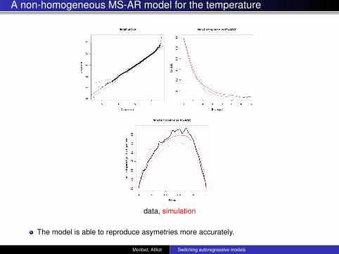
data, simulation

The model is able to reproduce asymetries more accurately.


A non-homogeneous MS-AR models for the temperatures

Durations in the regimes are no more geometric (especially in the 2nd regime)

Create more asymmetry in the dynamics


Some extensions

The model has been generalized to handleMultivariate time series

Applied to bivariate wind data ((u, v) components)Non linear autoregressive models

e.g. wind direction with von-Mises distribution

Other link functions


Flexibility of Non-homogeneous MS-AR models

Theoretical framework flexible enough to include models with exogenous covariates

For example non-homogeneous HMMs used for statistical downscaling

Covariates · · · → Zk−1 → Zk → Zk+1 → · · ·↘ ↘ ↘

Hidden Regime · · · → Xk−1 → Xk → Xk+1 → · · ·↓ ↓ ↓

Output time series · · · Rk−1 Rk Rk+1 · · ·

Covariates = large scale informationAssumed to be an ergodic Markov process

Output time series = local weather conditions(rainfall,temperature,...) at a meteorological station


Flexibility of Non-homogeneous MS-AR models

Some scientist argued that occurrence of longer anticyclonic conditions may be linked withsunspots.

Sunspots · · · → Zk−1 → Zk → Zk+1 → · · ·↘ ↘ ↘

Weather type · · · → Xk−1 → Xk → Xk+1 → · · ·↓ ↗ ↓ ↗ ↓

Temperatures · · · → Rk−1 → Rk → Rk+1 → · · ·


Non-homogeneous MS-AR model with sunspots

Sunspots · · · → Zk−1 → Zk → Zk+1 → · · ·↘ ↘ ↘

Weather type · · · → Xk−1 → Xk → Xk+1 → · · ·↓ ↗ ↓ ↗ ↓

Temperatures · · · → Rk−1 → Rk → Rk+1 → · · ·

Logistic link function for the switching probabilities. For s ∈ {1, 2},

P(St = s|St−1 = s,Yt−1 = yt−1,Zt−1 = zt−1)

= π(s)− +

1− π(s)− − π

(s)+

1 + exp(λ

(s)0 + λ

(s)1 yt−1 + λ

(s)2 zt−1

)


Transitions with sunspots

λ(1)2 : 1.82 [0.69, 3.80], λ(2)

2 : 1.35 [-1.13, 4.63]


MS-AR with sunspots

Sunspots, 1−max per month(duration of regime 1) NH MS-AR, NH MS-AR with sunspotsPearson’s correlation test p-value 0.03, with sunspots 1e−3


MS-AR with sunspots


Spatial model : MS-VAR

Spatio-temporal model at the scale of France : MS-VAR(2) with homogeneous or nonhomogeneous transition probabilities (covariable = temperature in Rennes).Same regime for all the sites.Does the model allow to "observe" motion of large scale events?


Spatial model : MS-VAR, NH MS-VAR

Cross-correlations

Homogeneous model

Non Homogeneous model


Spatial model : NH MS-VAR

Cross-correlations

Cold Regime

Hot Regime



Mean number of up-crossings

Homogeneous model




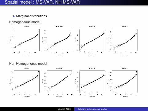
Marginal distributions

Homogeneous model




MS-VAR(2) spatio temporal models for temperatureallows to quite well reproduce

Marginal distributions (high temperature have to be improved...)Space-time correlation with delaySome non linearities (E(Nu))

The non homogeneous transition probabilities improve the results.


Conclusions

Weather type models provide a flexible and interpretable family of models formeteorological time seriesModels have been developed/validated for generating

(rainfall, temperature, solar radiation, humidity, wind speed) simultaneously at a singlelocation with a priori clusteringWind speed, wind direction, temperature independently at a single location with latentclusteringRainfall and temperature independently at several locations simultaneously with latentclustering

More works needed forDeveloping multi-site and multi-parameters generatorsImproving some aspects of existing models

Interannual variability underestimated ("overdispersion" phenomenon)Probability of long "events" (dry spell, heat wave,...) generally underestimated but can be improvedby introducing large scale covariate (e.g. sunspots)

R package under developmentReferences

Ailliot P., Monbet V., (2012), Markov-switching autoregressive models for wind time series.Environmental Modelling & Software, 30, pp 92-101.Ailliot P., Pène F. (2013), Consistency of the maximum likelihood estimate forNon-homogeneous Markov-switching models. Submitted.


Documents

Stochastic weather generators with non-homogeneous …pagesperso.univ-brest.fr/~ailliot/SlidesAber/Monbet_Aber.pdf · Stochastic weather generators with non-homogeneous hidden Markov