Embed Size (px)
Citation preview

Stochastic volatility models and hybrid
derivatives
Claudio Albanese
Department of Mathematics / Imperial College London
? ? ?
Presented at Bloomberg and at the Courant Institute, New
York University
New York, September 22nd, 2005

Co-authors.
• Oliver Chen
(National University of Singapore)
• Antonio Dalessandro
(Imperial College London)
• Manlio Trovato
(Merrill Lynch London)
available at:
www.imperial.ac.uk/mathfin
1

Contents.
• Part I. A stochastic volatility term structure model.
• Part II. Credit barrier models with functional lattices.
• Part III. Estimations under P and under Q.
• Part IV. Pricing credit-equity hybrids.
• PART V. Credit correlation modeling and synthetic CDOs.
• Part VI. Pricing credit-interest rate hybrids.
2

PART I. A stochastic volatility term structure model
It is widely recognized that fixed income exotics should be priced by
means of a stochastic volatility model. Callable constant maturity
swaps (CMS) are a particularly interesting case due to the sensitivity
of swap rates to implied swaption volatilities for very deep out of the
money strikes. In this paper we introduce a stochastic volatility term
structure model based on a continuous time lattice which allows for
a numerically stable and quite efficient methodology to price fixed
income exotics and evaluate hedge ratios.
3

Introduction
The history of interest rate models is characterized by a long series of
turns. The Black formula for caplets and swaptions was designed to
take as underlying a single forward rate under the appropriate forward
measure, see (Joshi & Rebonato 2003). This has the advantage to
lead to a simple pricing formula for European options but also the
limitation of not being extendable to callable contracts. To have a
more consistent model, short rate models where introduced in (Cox,
Ingersoll & Ross 1985), (Vasicek 1977), (Black & Karasinski 1991)
and (Hull & White 1993). These models are distinguished by the exact
specification of the spot rate dynamics through time, in particular the
form of the diffusion process, and hence the underlying distribution of
the spot rate.
4

LMM models
Next came LIBOR market models, also known as correlation models.
First introduced in (Brace, Gatarek & Musiela 1996) and (Jamshidian
1997), forward LIBOR models affirmed themselves as a mainstream
methodology and are now discussed in textbooks such as for instance
(Brigo & Mercurio 2001). Various extensions of forward LIBOR mod-
els that attempt to incorporate volatility smiles of interest rates have
been proposed. Local volatility type extensions were pioneered in
(Andersen & Andreasen 2000). A stochastic volatility extension is
proposed in (Andersen & Brotherton-Ratcliffe 2001), and is further
extended in (Andersen & Andreasen 2002). A different approach to
stochastic volatility forward LIBOR models is described in (Joshi &
Rebonato 2003). Jump-diffusion forward LIBOR models are treated
in (Glasserman & Merener 2001), (Glasserman & Kou 1999). A cali-
bration framework is proposed in (Piterbarg 2003).
5

Stochastic volatility models
Modeling stochastic volatility within LIBOR market models is a chal-
lenging task from an implementation viewpoint. In fact, Monte Carlo
methods tend to be slow and inefficient in the presence of a large num-
ber of factors. In a strive to achieve a more reliable pricing framework,
in recent years, we witnessed a move away from correlation models
and the emergence and recognition as market standard of the SABR
model by (S.Hagan, Kumar, S.Lesniewski & E.Woodward 2002) in the
fixed income domain.
6

SABR
SABR however is unlikely to be the definitive solution and is perhaps
rather just yet another stepping stone in a long chain. In fact, like-
wise to the Black formula approach, SABR takes up a single forward
rate under the corresponding forward measure as underlier. As a con-
sequence, within this framework it is not possible to price callable
swaps and Bermuda swaptions. There are also calibration inconsis-
tencies. Implied swaption volatilities with very large strikes are probed
by constant maturity swaps (CMS), structures which receive fixed, or
LIBOR plus a spread, and pay the equilibrium swap rate of a given
maturity. The asymptotic behavior of implied volatilities for very large
strikes turns out to flatten out to a constant, as opposed to diverging
rapidly as SABR would predict. Finally, some pricing inconsistencies
may emerge with SABR due to the fact that the model is solved by
means of asymptotic expansions with a finite, irreducible error.
7

Stochastic volatility term structure models
In this article we attempt to go beyond SABR by introducing a stochas-
tic volatility short rate model which has the correct asymptotic behav-
ior for implied swaption volatilities and can be used for callable swaps
and Bermuda swaptions. Our model is solved efficiently by means of
numerical linear algebra routines and is based on continuous time lat-
tices of a new type. No calculation requires the use of Montecarlo or
asymptotic methods and prices and hedge ratios are very stable, even
for extreme values of moneyness.
8

Nearly stationary calibration
Our model is made consistent with the term structure of interest rates
and the term structure of implied at-the-money volatilities by means
of a calibration procedure that greatly reduces the degree of time
dependency of coefficients. As a consequence, the model is nearly
stationary over time horizons in excess of 30 years.
9

Applications
In this presentation, I discuss the model by reviewing in detail an
implementation example. While leaving it up to the interested reader
to pursue the many conceivable variations and extensions, we describe
the salient features of our modeling by focusing in detail to the problem
of pricing and finding hedge ratios for Bermuda swaptions and callable
CMS swaps.
10

The model
Our model is built upon a specification of a short rate process rt
which combines local volatility, stochastic volatility and jumps. We
make our best effort to calibrate the model to a stationary process
and introduce the least possible degree of explicit time dependence in
such a way to refine fits of the term structure of interest rates and of
selected at-the-money swaption volatilites. The model is specified in
a largely non-parametric fashion within a functional analysis formalism
and expressed in terms of continuous time lattice models.
A sequence of several steps is required to specify the short rate process
rt.
11

The conditional local volatility processes
We introduce M states of volatility. The process conditioned to stay
in one of such states α ∈ 1, ...M is related to the solution rαt of the
following equation:
drαt = κα(θα − rαt)dt + σαrβααt dW. (1)
12

Short rate volatilities for each of the four volatility states
13

The functional analysis formalism
In the functional analysis formalism we use, these SDEs are associated
to the Markov generators
Lrα = κα(θα − rαt)
∂
∂r+
σ2αr
2βααt
2
∂2
∂r2. (2)
14

Functional lattices
To build a continuous time lattice (also called functional lattice), we
discretize the short rate variable and constrain it to belong to a finite
lattice Ω containing N +1 points r(x) ≥ 0, where x = 0, ...N , r(0) = 0
and the following ones are in increasing order. The discretized Markov
generator LrΩα is defined as the operator represented by a tridiagonal
matrix such that ∑yLr
Ωα(x, y) = 0∑yLr
Ωα(x, y)(y − x) = κα(θα − r(x))∑yLr
Ωα(x, y)(y − x)2 = σ2αr(x)2βα.
15

Model parameters
In our example, we select an inhomogeneous grid of N = 70 points
spanning short rates from 0% to 50%. We also choose to work with
M = 4 states for volatility and make the following parameter choices:
α σα βα θα κα
0 31% 30% 2.10% .171 46% 40% 5.50% .182 75% 50% 8.50% .233 100% 60% 12.00% .24
16

How to solve in the special case of a local volatility model (M=1)
and without jumps
Although our model is more complex than a simple local volatility
process, it is convenient to describe our resolution method in the
specific case of the operator LrΩα with constant α. This method can
then be generalized and is at the basis of other extensions such as the
introduction of jumps (see below).
17

Spectral analysis
We start by considering the following pair of eigenvalue problems:
LrΩαun = λnun LrT
Ωαvn = λnvn
where the superscript T denotes matrix transposition, un and vn are
the right and left eigenvectors of LrΩα, respectively, whereas λn are the
corresponding eigenvalues. Except for the simplest cases, the Markov
generator LrΩα is not a symmetric matrix, hence un and vn are different.
18

Spectral analysis
Also, in general the eigenvalues are not real. We are only guaranteed
that their real part is non-positive Reλn ≤ 0 and that complex eigen-
values occur in complex conjugate pairs, in the sense that if λn is an
eigenvalue then also λn is an eigenvalue. We set boundary conditions
in such a way that there is absorption at the endpoints, and in par-
ticular at the point corresponding to zero rates r(0) = 0. With this
choice, we are also guaranteed that there exists a zero eigenvalue.
19

Spectral analysis
There is no guarantee, in the most general case, that there exists
a complete set of eigenfunctions. However, the chance that such a
complete set does not exist for a Markov generator specified non-
parametrically is zero, so we can safely assume that this is the case.
In the unlikely case that this assumption is not correct, the numerical
linear algebra routines needed to solve our lattice model will identify
the problem and a small perturbation of the given operator will suffice
to rectify the situation. Assuming completeness, the diagonalization
problem can be rewritten in the following matrix form:
LrΩα = UΛU−1 (3)
where U is the matrix having as columns the right eigenvectors and Λ
is the diagonal matrix having the eigenvalues λi as elements.
20

Functional calculus
Key to our constructions is the remark that, if the Markov generator
is diagonalisable, we can apply an arbitrary function F to it by means
of the following formula:
F (LrΩα) = UF (∗r
Ωα)U−1 (4)
This formula is at the basis of the so-called ”functional calculus”.
As Ito’s formula regarding functions of stochastic processes is central
in the mathematical Finance for diffusion processes, functional cal-
culus for Markov generators plays a pivotal role in our framework for
stochastic volatility models.
21

Functional calculus
This formula has several applications. An immediate one allows us to
express the pricing kernel u(r(x), t; r(y), T ) of the process as follows:
u(r(x), t; r(y), T ) = (e(T−t)LrΩα)(x, y) =
∑n
eλn(T−t)un(x)vn(y). (5)
22

Introducing jumps
At this stage of the construction one has the option to also add jumps.
Although in the example discussed in this paper we are mostly focused
on long dated callable swaps and swaptions for which we find that the
impact of jumps can be safely ignored, adding jumps involves negligible
additional complexities and is thus worth considering and implement-
ing in other situations. To add jumps, one can follow the following
procedure which accounts for the need to assign different intensities
to up-jumps and down-jumps. Jump processes are associated to a
special class of stochastic time changes given by monotonously non-
decreasing processes Tt with independent increments.
23

Stochastic time changes
The time changes characterizing Levy processes with symmetric jumps
are known as Bochner subordinators and are characterized by a Bochner
function φ(λ) such that
E0
[e−λTt
]= e−φ(λ)t (6)
24

The variance-gamma model
For example, the case of the variance gamma process which received
much attention in Finance corresponds to the function
φ(λ) =µ2
νlog
(1 + λ
µ
ν
)(7)
where µ is the mean rate and ν is the variance rate of the variance
gamma process.
25

The generator of the jump process
The generator of the jump process can be expressed using functional
calculus as the operator −φ(−LrΩα). To produce asymmetric jumps,
we specify the two parameters differently for the up and down jumps
and compute separately two Markov generators
L± = −φ±(−LrΩα) = −U±φ±(Λ)V± (8)
where:
φ±(λ) =µ2±
ν±log(1 + λ
µ±ν±
) (9)
26

The generator of the process with asymmetric jumps
The new generator for our process with asymmetric jumps is obtained
by combining the two generators above
LrjΩα =
0 · · · · · · · · · 0
L−(2,1) d(2,2) L+(2,3) · · · L+(2, n)... ... . . . · · · ...
L−(n− 1,1) L−(n− 1,2) · · · d(n− 1, n− 1) L+(n− 1, n)0 0 · · · · · · 0
27

Probability conservation and boundary conditions
Here the element of the diagonal are chosen in such a way to satisfy
probability conservation:
d(x, x) = −∑y 6=x
LrjΩα(x, y) (10)
Also notice that we have zeroed out the elements in the matrix at the
upper and lower boundary: this ensures that there is no probability
leakage in the process.
28

Drift condition
In our setting, we choose a short rate as a modeling primitive and
we thus do not need to impose a martingale condition. Otherwise,
were we working with a forward rate instead, the appropriate method
of restoring the martingale condition would be to modify the matrix
elements of the resulting generator on the first sub-diagonal and the
first super-diagonal.
29

The Local Levy generator
At this stage of the construction, we have therefore obtained a gener-
ator LrjΩα for the short rate process, whose dynamics is characterized
by a combination of state dependent local volatility and asymmetric
jumps. We note that the addition of jumps has not increased the di-
mensionality of the problem and is therefore computationally efficient.
30

Modeling the dynamics of stochastic volatility
As a third step, we define a dynamics for stochastic volatility by as-
signing a Markov generator to the volatility state variable α which
depends on the rate coordinate x. Namely, conditioned to the rate
variable being x, the generator has the following form
Lsvx = ε(x)Lsv
+ + Lsv− (11)
where
Lsv+ =
−0.7 0.7 0 0
0 −1.1 0.8 0.30 0 −1.5 1.50 0 0 0
, Lsv− =
0 0 0 0
1.4 −1.4 0 00 3 −3 00 0 5 −5
.
(12)
31
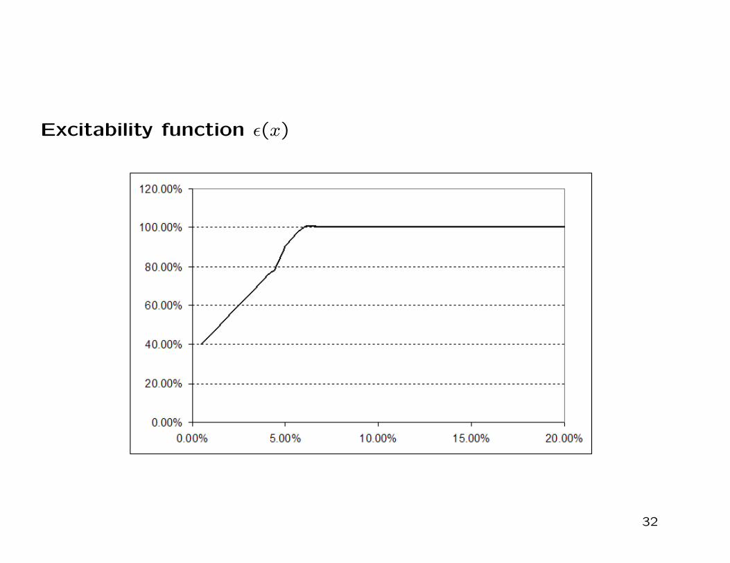
Excitability function ε(x)
32

The total generator
Out of the two generators we just defined, we form a Markov generator
L acting on functions of both the rate variable x and the volatility
variable α. This generator has matrix elements given as follows:
L(x, α; y, β) = LrjΩα(x, y)δα,β + Lsv
x (α, β)δxy. (13)
33

Numerical analysis
In our working example, the matrix L has total dimension MN = 280.
For matrices of this size, diagonalization routines such as dgeev in
LAPACK are very efficient. Since our underlier is a short rate though,
we are not interested in the pricing kernel but rather in the discounted
transition probabilities given by
p(x, t; y, T ) = E
[e−∫ Tt rsds, |rt = r(x), rT = r(y)
]. (14)
34

Numerical analysis
This kernel satisfies the following backward equation
∂
∂tp(x, t; y, T ) + (Lp)(x, t; y, T ) = r(x)p(x, t; y, T ). (15)
In functional calculus notations, the solution is given by
p(x, t; y, T ) = eG(T−t)(x, y) where G(x, y) ≡ L(x, y)− r(x)δxy.
(16)
35

Numerical analysis with stochastic volatility
The same diagonalization method illustrated above for the local volatil-
ity case applies also in this situation. By representing the matrix G in
the form
G = UΛU−1 (17)
where Λ is diagonal, and writing the matrix of discounted transition
probabilities as follows
eG(T−t) = UeΛ(T−t)U−1. (18)
36

Calibration and Pricing
In our example, to calibrate our model we aim at matching forward
swap rates and at-the-money swaption volatilities, both referring to
swaps of 5 year tenor. We start from the following data
1y 2y 3y 4y 5y 7y 10y 15y 20y 30yforward 2.999% 3.311% 3.587% 3.800% 3.984% 4.226% 4.393% 4.477% 4.301% 4.114%ATM vol 21.506% 19.443% 17.962% 16.967% 16.189% 14.897% 13.801% 12.460% 12.665% 11.728%
37

Nearly stationary calibration
The calibration procedure has two steps. In a first step we search for
a best fit using the model above without introducing any explicit time
dependency. In a second step, we then introduce time dependency to
achieve a perfect fit. As a consequence of this procedure, the degree
of time variability of model parameters is kept to a bare minimum.
To introduce time dependence we combine two operations: a shift of
the short rate by a time varying, deterministic function of time and a
deterministic time change, i.e.
rt → rt = b(t)rb(t) + a(t). (19)
38

Nearly stationary calibration
Here b(t) is monotonously increasing and b(t) denotes its time deriva-
tive. Using the new process, discounted transition probabilities can be
computed as follows:
E
[e−∫ Tt rsds, |rt = r(x), rT = r(y)
]= e−
∫ Tt a(s)dsG(x, b(t); y, b(T )) (20)
where G is the kernel for the stationary process defined above.
Our choice in the working example is b(t) = 1.095t + 0.008t2. The
function a(t) is then defined in such a way to match the term structure
of forward swap rates. This adjustment is given in the next slide.
39

Deterministic yield adjustment (EUR)
40

Degree of time dependence
As one can see from this picture, the yield adjustment is less than 20
basis points in absolute value. This ensures that the probability of the
modified short rate process rt to attain negative values is small. In a
typical implementation of the Hull-White model along similar lines, the
short rate adjustment is typically of a few percent. The discrepancy
is linked to the fact that the richer stochastic volatility model we
construct is capable of explaining most of the salient features of the
zero curve even with the constraint that the process be stationary.
41
Advantages of nearly stationary model calibration
The advantage of having a nearly stationary model is that the shapes
of yield curves that one obtains depend on the short rate and the
volatility state but are largely independent of time. The figure in
the next slide shows the yield curves corresponding to different initial
volatility states and different starting values for the short rate. As
the graphs indicate, yield curves are sensitive to the initial volatility
state as they raise if initial volatilities raise. Moreover graphs show
that curves invert for high values of the short rate. In our model, this
behavior is consistent over all time frames except for corrections of
the order of 10 basis points.
42

Yield curves for different values of the initial volatility state and
of the short rate
43

Pricing swaptions and callable constant maturity swaps
Implied volatilities for European swaptions are given in the next slide.
Here we graph extreme out of the money strikes of up to 15% for
swaptions of varying maturities where the deliverable is a 5Y swap.
One can notice that implied volatilities naturally flatten out at long
maturities, a behavior consistent with what observed in the CMS mar-
ket where such extreme strike levels are probed.
44

Implied volatility for European swaptions (EUR)
45
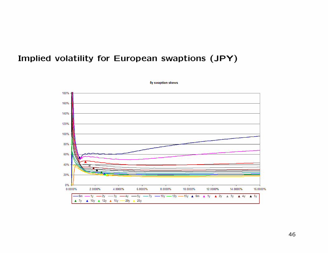
Implied volatility for European swaptions (JPY)
46

Term structure of implied 5Y swaption volatilities (JPY)
47

Bermuda swaptions
Exercise boundaries for 10Y Bermuda swaptions are given in the next
slides. The first graph refers to payer swaptions and the second to
receiver swaptions.
48

Exercise boundaries for payer Bermuda options
49

Exercise boundaries for receiver Bermuda options
The corresponding graphs for callable CMSs are given below. Notice
that the exercise boundaries depend on the volatility state.
50

Exercise boundaries for callable payer CMSs
51

Exercise boundaries for callable receiver CMSs
52

Sensitivities for Bermuda swaptions
Sensitivities for Bermuda swaptions are given in the next slides. These
sensitivities are computed by holding the volatility state variable fixed
and are defined as the derivative of the price for a 10Y payer Bermuda
swaption with respect to the rate of the 10Y swap.
53

Delta of a 10Y Bermuda swaption, with semi-annual exercise
schedule, with respect to the 10Y swap rate. This is computed
while holding fixed the volatility state variable.
54

Gamma of a 10Y Bermuda swaption, with semi-annual exercise
schedule, with respect to the 10Y swap rate. This is computed
while holding fixed the volatility state variable.
55
Sensitivities for Constant Maturity Swaps
Sensitivities of callable constant maturity swaps are given in the next
slides. The delta and gamma are computed similarly to what done for
Bermuda swaptions, while the vega is calculated instead with respect
to the 10Y into 5Y European swaption.
56
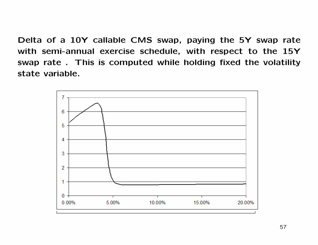
Delta of a 10Y callable CMS swap, paying the 5Y swap rate
with semi-annual exercise schedule, with respect to the 15Y
swap rate . This is computed while holding fixed the volatility
state variable.
57

Gamma of a 10Y callable CMS swap, paying the 5Y swap rate
with semi-annual exercise schedule, with respect to the 15Y
swap rate. This is computed while holding fixed the volatility
state variable.
58

Vega of a 10Y callable CMS swap, paying the 5Y swap rate with
semi-annual exercise schedule, with respect to the 10Y into 5Y
European swaption price. This is computed while holding fixed
the short rate.
59

Conclusions
We present a stochastic volatility term structure model, providing a
consistent framework for pricing European and Bermuda options, as
well as callable CMS swaps. The model is built upon a specification
of a short rate process, which combines local volatility, stochastic
volatility and jumps. The richness of the model allows to keep the
degree of time variability of model parameters to a bare minimum,
and obtain a nearly stationary behaviour. The solution methodology
is based on a new type of continuous time lattices, which allow for a
numerically stable and quite efficient technique to price fixed income
exotics and evaluate hedge ratios.
60

PART II. Credit Barrier Models
Statistical data that we would like a credit model to fit includes:
• historical default probabilities given an initial credit rating
• historical transition probabilities between credit ratings
• interest rate spreads due to credit quality
61

Credit-rating based models
The early models of this class considered the credit-rating migration
and default process as a discrete, time-homogenous Markov chain
and took the historical transition probability matrix as the Markov
transition matrix.
Deficiencies:
• difficult to correlate
• risk-neutralization leads to unintuitive results
62

Analytic closed form solutions versus numerical linear algebra
methods
The former framework for credit barrier models leveraged on solvable
models.
In the newer version recently developed we have a flexible non-parametric
framework, whereby tractability comes from the use of numerical lin-
ear algebra as opposed to coming from the analytical tractability of
special functions.
63

The underling diffusion process
The first building block of our construction is a Markov chain process
xt on the lattice Ω = 0, h, ..., hN ⊂ [0,1] where N is a positive integer
and h = 1/N . In the case of a discretized diffusion with state depen-
dent drift and volatility, the infinitesimal generator L, of the process
xt is a tridiagonal matrix and can be expressed as follows in terms of
finite difference operators:
Lx = a(x)∆ + [b(x)− a(x)]∇+
where x ∈ Ω and
(∆f)(x) = f(x+1)+f(x−1)−2f(x), and (∇+f)(x) = f(x+1)−f(x).
(21)
64

Continuous space limit
To ensure the existence of a continuous space limit, we derive the
functions a(x), b(x) from a drift function µ(ξ) and a volatility function
σ(ξ), where ξ ∈ [0,1], which is identifiable as the credit quality process
and can be expressed in terms of its infinitesimal by imposing the
following conditions: ∑y L(x, y)(y − x) = µ(hx)∑y L(x, y)(y − x)2 = σ(hx)2∑
y L(x, y) = 0
65
The P and the Q measure
In our model, we actually use two drift functions: µP (ξ) and µQ(ξ),
one defining the P or statistical measure and the latter modeling the Q
or pricing measure. We postulate that the only difference between the
P and the Q measure lies in the specification of these two drift func-
tions. Correspondingly, we use the subscripts P and Q to identify the
Markov generator and transition probabilities under the corresponding
measure. Whenever the subscripts are omitted as here below, formulas
apply to both the P and the Q measure.
66

Eigenvalue problems and functional calculus
To manipulate the Markov generator by means of functional calculus,
the first step is to diagonalize it. Let λn be the eigenvalues of the
operator L and let un(x) and vn(x) be the right eigenvectors, so that
Lun = λnun.
67

Numerical methods for eigenvalue problems
In most cases, Markov generators admit a complete set of eigenvec-
tors. Although there are exceptions where diagonalization is not pos-
sible and one can reduce the operator at most to a non trivial Jordan
form with non-zero off-diagonal elements, these exceptional situations
occur very rarely both in a measure theoretic sense, as exceptions span
a set of zero measure, and in a topological sense as their complement
is dense in the space of all generators. In practical terms, this implies
that non-diagonalizable operators arise very rarely if at all in practice
and whenever they do, a professional numerical diagonalization algo-
rithm would detect the problem and a small perturbation of the model
parameters would rectify. To carry out numerical diagonalization, we
find that the function dgeev in the public domain package LAPACK is
quite suitable.
68
Diagonalizing the Markov generator
We just assume that the operator L admits a complete set of eigen-
vectors. In this case, we can form the matrix U whose columns are
given by the eigenvectors un(x) and write
L = UΛU−1. (22)
We denote with V the operator U−1 and with vn(x) its row vectors.
69

Functional calculus
Key to our constructions is the remark that if the matrix operator Lis diagonalizable we can apply an arbitrary function F to it by means
of the following formula:
F (L) = UF (Λ)U−1 (23)
This formula is at the basis of the so-called ”functional calculus”. As
Ito’s formula regarding functions of stochastic processes is central in
the stochastic analysis for diffusion processes, functional calculus for
Markov generators plays a pivotal role in our framework for stochastic
volatility models. This formula has several applications. An immediate
one allows us to express the pricing kernel u(x, t; y, t′) of the process
as follows:
u(x, t; y, t′) = (e(t′−t)L)(x, y) =
∑n
eλn(t′−t)un(x)vn(y). (24)
70

Introducing jumps
At this stage of the construction we add jumps. Jumps are ubiquitous
in credit model and we find that a jump component is necessary in
order to reconcile observed default probabilities with credit migration
probabilities. Within our framework, adding jumps involves marginal
additional complexities from the numerical viewpoint.
71

Asymmetric jumps
To reflect asymmetries in the jump intensities, we model separately
up and down jumps. A particularly interesting class of jump processes
is associated to stochastic time changes given by monotonously non-
decreasing processes Tt with independent increments. These time
changes are known as Bochner subordinators and are characterized by
a Bochner function φ(λ) such that
E0
[e−λTt
]= e−φ(λ)t (25)
For example, the case of the variance gamma process which received
much attention in Finance corresponds to the function
φ(λ) =µ2
νlog
(1 + λ
µ
ν
)(26)
where µ is the mean rate and ν is the variance rate of the variance
gamma process.
72

Functional calculus with subordinated generators
The generator of the jump process corresponding to the subordination
of a process of generator L can be expressed using functional calculus
as the operator −φ(−L). To produce asymmetric jumps, we specify
the two parameters differently for the up and down jumps and compute
separately two Markov generators
L± = −φ±(−L) = −U±φ(−Λ±)V± (27)
where:
φ±(λ) =µ2±
ν±log
(1 + λ
µ±ν±
)(28)
73

Generators with asymmetric jumps
The new generator for our process with asymmetric jumps is obtained
by combining the two generators above
L =
0 · · · · · · · · · 0
L−(2,1) d(2,2) L+(2,3) · · · L+(2, n)... ... . . . · · · ...
L−(n− 1, n) L−(n− 1,2) · · · d(n− 1, n− 1) L+(n− 1, n)0 0 · · · · · · 0
Here the element of the diagonal are chosen in such a way to satisfy
the condition of probability conservation
d(i, i) = −∑j 6=i
L(i, j) (29)
Also notice that we have zeroed out the elements in the matrix at the
upper and lower boundary: this ensures that there is no probability
leakage in the process.
74

Adding jumps
At this stage of the construction, we have therefore obtained a gen-
erator Lj for the process of distance to default, whose dynamics is
characterized by a combination of state dependent local volatility and
asymmetric jumps. We note that the addition of jumps has not in-
creased the dimensionality of the problem and is therefore computa-
tionally efficient.
75

PART III: Estimation and calibration: P measure
We first estimate the process for distance to default xt with respect to
the statistical measure P by matching transition probabilities over one
year and default probabilities over time horizons of 1, 3 and 5 years.
A credit rating system consists of a number K of different classes. In
the case of the extended system by Moody’s, K = 18 and the ratings
are:
0,1, . . . ,17 ↔ Default,Caa,B3,Ba3,Ba2, . . . ,Aa3,Aa2,Aa1,Aaa
76

Introducing barriers
We subdivide the nodes of the lattice Ω into K subintervals of adjacent
nodes:
Ii = [xi−1, ...xi] (30)
where 0 = x0 < x1 < ... < xK = N and #(xi − xi−1) = NK , for i =
1, ..., K. The interval Ii corresponds to the i-th rating class. If a
process is in Ii at time t, then is said to have a credit rating of i. ∀i,
xi ∈ Ii denotes the initial node. The conditional transition probability
pij(t) that an obligor with a given initial rating i at time 0 will have
a rating j at a later time t > 0 can be estimated by matching it with
historical averages provided by credit assessment institutions.
77

Introducing barriers
For our purposes, we model this quantity as follows:
pij(t) =
aj−1∑y=aj−1
uP (0, xi; t, y).
where xi is a point in the interval Ii which represents the barycenter
of the population density in that credit class and is part of the model
specification. For simplicity’s sake, we take xi to be the midpoint of
the interval Ii.
78

The state of default
Absorption into the state x = 0 is interpreted as the occurrence of
default. The probability that starting from the initial rating i and
reaching a state of default by time t is given by
pDi (t) = uP (0, xi; t,0).
The model under P is characterized by a drift function µP (ξ), a
volatility function σ(ξ) and jump intensities. The first two func-
tions are graphed below, while the variance rates we estimated are
ν+ = 7.5, ν− = 4.
79

Local volatility σ(ξ) vs. distance to default
80

Local drifts µP (ξ) and µQ(ξ) vs distance to default under the P
and the Q measure, respectively.
81

Comparison of discrete model (lines) and historical (dots) one
year transition probabilities.
82

Comparison of discrete model (lines) and historical (dots) de-
fault probabilities.
83

Estimation and calibration: Q measure
Risk neutralization is defined by changing the drift function µP (ξ) into
µQ(ξ), while leaving everything else unaltered.
The new drift is chosen in such a way to fit spread curves. Term
structures of probability of default for each rating class are given by
qDi (t) = uQ(0, xi; t,0). (31)
84

CDX index spreads
In our example, we use CDS spreads for 125 names in the Dow Jones
CDX index. We looked at 5 datasets by Mark-it Partners correspond-
ing to the last business days of the months of January, February,
March, April and May 2005. The datasets provide CDS spreads at
maturities: 6m, 1y, 2y, 3y, 5y, 7y, 10y and tentative recovery rates for
each name. We insist that the CDS spreads be matched by our model
and take the liberty of adjusting the term structure of recovery rate
for each name. Besides having to estimate the drift under Q we also
estimate the current distance to default for each name. The objective
is to ensure that the term structure of recovery rates be as flat as
possible and as close as possible to the tentative input value.
85

Comparison of discrete model (lines) and market (dots) for
spread curves of investment grade bonds (Data taken 02/10/2003)
86

Comparison of discrete model (lines) and market (dots) for
spread curves of speculative grade bonds (Data taken 02/10/2003)
87

Liquidity spreads
From these pictures one can notice a systematic bias in spreads. Our
model appears to systematically underestimate BB spreads and over-
estimate BBB spreads.
This can be interpreted in terms of the differential liquidity in the two
market sectors.
88

CDS Spreads: Investment Grades (Data from March 2005)
89

CDS Spreads: Non-Investment Grades (Data from March 2005)
90

Implied term structure of recovery rates
We observe that the implied term structures of recovery rates are
highly correlated across names and to the general spread level. This is
not surprising as recovery levels are known to be linked to the economic
cycle. Hence implied recoveries reflect the market perception of the
future economic cycle. As we compare the implied recovery cycles
on the last business day of January, March and May 2005, we notice
that the implied recovery cycle appears equally pronounced in the three
months. However, the ones in January and March show a much greater
degree of coherence across names, perhaps a signature of the fact that
in January and March markets were rather tranquil and efficient, while
in May 2005 dislocations occurred.
91
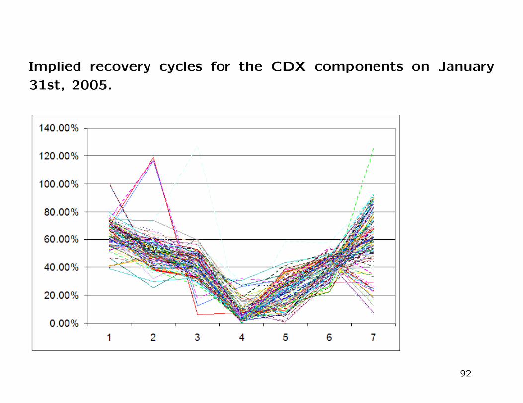
Implied recovery cycles for the CDX components on January
31st, 2005.
92

Implied recovery cycles for the CDX components on March 31st,
2005.
93

Implied recovery cycles for the CDX components on May 31st,
2005.
94

Risk-neutral transition probabilities
In the risk-neutral setting we can also calculate risk-neutral transition
probabilities. These are necessary to price credit-rating dependent
options.
How do we expect risk-neutral transition probabilities to behave? In-
dependent of the model, since risk-neutral default probabilities are
greater than historical default probabilities, one would expect down-
grades in credit-rating to be more probable in the risk-neutral setting
than historically.
95

96

97

98

PART IV. Equity default swaps (EDS)
Equity default swaps are a new class of instruments that several dealers
started marketing this year. They are defined as out of the money
American digital puts struck at 30% of the spot price. Typical maturity
is 5 years and the premium is paid in installments by means of a semi-
annual coupon stream.
In this example, I will compare CEV prices with the prices one obtains
from credit barrier models. The latter, are models estimated to ag-
gregate data, namely the credit transition matrix, default probabilities
and credit spread curves. The credit equity mapping is obtained by
fitting at-the-money implied volatilities as a function of the ratings.
99

Main Finding
It appears that the market is currently pricing EDSs by means of
diffusion local volatility models and that this is not entirely consistent
with credit derivative data. The marked differences in prices are due
to the fact that the credit barrier model accounts for the phenomenon
of ”fallen angels” by introducing and calibrating a jump component in
the process.
100

Credit-Equity mapping
101

Mapping to equity
The credit quality is mapped to equity prices via a deterministic, mono-
tonic function Φ at some horizon date T :
ST (ζ) = erTΦ(ζ)
For ti < T , we take the discounted expectation of Φ:
Sti(ζ) = ertiE[Φ(ζ)|ζti]
102

A snapshot of market EDS spreads
103

Credit quality versus stock price (the credit equity mapping)
104

Local volatility
105
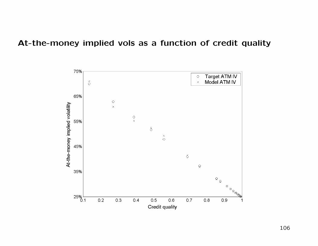
At-the-money implied vols as a function of credit quality
106

EDS spreads as a function of rating
107

CDS to EDS spread ratio as a function of rating
108

CDS to EDS spread ratio based on the CEV model
109

PART V. Credit correlation modeling and lattice models for
synthetic CDOs.
Having characterized the process for credit quality xt and identified
starting points for each individual procsess, the next step is to in-
troduce correlations by conditioning to economic cycle scenarios, thus
introducing a correlation structure among the credit quality processes.
The economic cycle is modeled by means of a non-recombining lat-
tice of the structure sketched below. The underlying index variable is
allowed to take up two values on each period ∆t. An upturn corre-
sponds to a ”good” period while a downturn to a ”bad” period for
the economy. In our example, we chose the time step to be ∆t = 1y
and find that this choice is sufficient to provide great flexibility in the
tuning of the correlation structure.
110

Conditioning the Lattice to a Market Index
To explain our methodology to introduce correlations, we consider
first a simple case whereby the model is characterized by a pair of
complementary transition probabilities w, (1−w) ∈ [0,1] at each node,
which we assume constant. In order to condition the continuous time
lattice corresponding to a given credit quality process to the economic
index variable we introduce the notion of local beta given by function
β(ξ) which provides the corresponding sensitivity. The limiting cases of
β(ξ) = 0 and β(ξ) = 1 correspond to zero and full correlation between
a name with a given credit quality hx ∈ [0,1] and the cycle variable.
Along the path of each given scenario on the tree, the unconditional
kernel of the credit quality process is replaced by conditional transition
probabilities defined as follows:
u±w,β(t, x; t + ∆t, y) = (1− β(hx))u0(t, x; t + ∆t, y) + β(hx)u±1 (t, x; t + ∆t, y)
111

Here u0 = u is the unconditional kernel and corresponds to a zero
β(hx). In the opposite case of β(hx) = 1, conditional kernel u±1 (x, y)
has the following form:
u+1 (x, y) =
1
1− w
u(x, y) if y > m(w, x)(w −
∑y>m(w,x) u(x, a(w, x))
)if y = m(w, x)
u(x, y) = 0 if y < m(w, x)
(32)
and
u−1 (x, y) =1
w
0 if y > m(w, x)
u(x, m(w, x))− u+1 (x, m(w, x)) if y = m(w, x)
u(x, y) if y < a(w, x).
(33)
where
m(w, x) = inf
m = 0, ...N |
∑y<m
u(x, y) ≤ w
. (34)
Notice that, for all specifications of β(ξ) and w ∈ [0,1], we have that
u(x, y) = wu−β (x, y) + (1− w)u+β (x, y). (35)
Conditioning is achieved by forming a weighted sum over all paths in
the event tree. On a given path, we use u−β for a bad period scenario
and u+β for a good one. The weight of a path is the product of
a number of factors w equal to the number of bad periods and a
number of factors (1−w) for each one of the good periods. With this
method, marginal probabilities are kept unchanged while correlations
are induced on the single name processes. More specifically, one can
price all credit sensitive instruments specified with the given names one
can first evaluate the conditional prices PΓ by means of the following
multiperiod kernel:
e(ti−ti−1)Lγi · . . . · e(tn−tn−1)Lγi.

where Γ = γ1, . . . , γn runs over the sets of conditional paths due to
the scenario of the index. The (unconditional) price is then given by:
P =∑Γ
wn−(Γ)(1− w)n+(Γ)PΓ.
This construction can be generalized. Consider a number M > 1 of
percentile levels 0 < w1 < ... < wM < 1 and let qi ∈ [0,1], i = 1...M be
a corresponding set of probabilities summing up to one, i.e.∑
i qi = 1.
Then we can set
u±−→w ,β(t, x; t + ∆t, y) =
M∑i=1
qiu±wi,β
(t, x; t + ∆t, y). (36)
The formulas above extend also to this case as long as one replaces
the weight w with the average weight∑
i qiwi.
The choices we make for the March and June datasets are graphed
below. Here one can observe that the levels we were led to choose in

June are lower and the probabilities more uneven than in March. This
can be interpreted as saying that the model is detecting a higher level
of implied correlation between jumps in the June data than in March.

Specifications for the weights qi and percentile levels wi.
112

The local beta function
Modeling correlation is key to pricing basket credit derivatives. Buyers
and sellers of basket credit derivatives have a wide range of arbitrage-
free prices to choose from, and it is the market that determines, both in
principle and in practice, a definite price. In our framework, tranches
of varying seniority are priced by calibrating the local beta function
β(ξ).
113

Specifications for the function β(x) in March and June 2005.
114

Decoupling of correlation
Notice that as an effect of GM and Ford being downgraded, the local
beta function responded by lowering on the side of low quality grades
while rising on the high qualities. This resulted in a simultaneous fall
of equity prices and widening of senior spreads.
115

Contagion skew
A useful graph to assess the impact of the specification of the local
β(ξ) function on our correlation model is the contagion skew in the
next slide. This graph is constructed as follows: we first compute the
unconditional default probabilities as a function of credit quality. Next,
for each value of credit quality, assuming that a name of that quality
defaults within a time horizon of 5 years, we compute the conditional
probability of defaults for all other name. Finally, we take an average
over all values of credit quality of the ratio between the conditional
and unconditional probabilities. As the graph shows, the higher is the
credit quality of a defaulted name, the larger is the impact on all other
names. The steepness of this curve controls precisely the discrepancy
between prices for senior tranches as compared to junior ones.
116

Contagion Skew: ratio between conditional and unconditional
probability of defaults, where conditioning is with respect to the
default of a name whose credit quality is on the X axis.
117

Pricing CDOs
Although CDX index tranches are written on 125 underlying names, we
observe that our lattice model performs quite efficiently. We separate
the numerical analysis in two different steps. In the first we go through
all names and generate conditional lattices. We choose ∆t = 1y and a
time horizon of 5y, so that we obtain a total of 32 scenarios. This is a
pre-processing step which is independent of the CDO structure. This
step typically takes a few minutes for a hundred names and could
be carried out periodically and offline for the universe of all traded
names. The pricing step instead takes only a few seconds and requires
generating the probability distribution function for CDO portfolios over
the given time horizon.
118

Expected Loss Distribution for CDX index tranches in March
2005
119

Expected Loss Distribution for CDX index tranches in June 2005
120

Pricing CDOs
The model can be calibrated by adjusting the function β(ξ), ξ ∈ [0,1],
the thresholds wi, i = 1, ...M and the corresponding probabilities qi.
121

Tranche prices for March 20th 2005
attachment detachment spread mktspread0% 3% 499.6 bp (+32% uff) 500 bp(+32% uff)3% 6% 187.4 bp 189bp6% 9% 108.6 bp 64bp9% 12% 56.5 bp 22bp12% 22% 6.7 bp 8bp
where ”uff” stands for ”upfront fee”.
122

Calibration
Notice that a good agreement can be reached with the equity, junior
mezzanine and senior tranche. On the other hand, the model appears
to over-estimate the price of the two senior mezzanine tranches 6-9
and 9-12 by a factor 2-3. This might be in relation to the high degree
of liquidity of these tranches and appetite for this risk profile.
123

Tranche prices for June 20th 2005
attachment detachment spread mktspread0% 3% 499.7 bp (+49% uff) 500 bp(+49% uff)3% 6% 170.1 bp 177bp6% 9% 30.4 bp 54bp9% 12% 27.5 bp 24bp12% 22% 10.0 bp 12bp
124

Hedge ratios of the various CDO tranches for March 2005 plot-ted against 5Y CDS spreads.
125

Hedge ratios.
One can notice that the hedge curves for the equity and the junior
mezzanine are fairly different and as a consequence it does not appear
as appropriate to use the mezzanine as a proxy to hedge credit expo-
sure at the equity tranche level. The differentiation among the two
profiles is a direct consequence of the steep aspect of the local beta
function.
126

Conclusions
We propose a novel approach to dynamic credit correlation modeling
that is based on continuous time lattice models correlated by con-
ditioning to a non-recombining tree. The model describes not only
default events but also rating transitions and spread dynamics, while
single name marginal processes are preserved.
127

PART VI. Credit-interest rate hybrids
Functional lattices for the dynamic CDO model and for the term struc-
ture model covered above can be combined and correlated while pre-
serving the specification of marginal processes. This opens the possi-
bility of pricing credit - interest rate hybrid instruments.
As an example of these applications, in the following, we consider
cancellable interest rate swaps which are linked to the default of either
one name in the CDX index, or to the first default event of a name
in a given basket, or to the default of the CDX equity tranche. We
also consider interest floors that cancel upon the default of the equity
tranche. In all cases, we evaluate also hedge ratios.
128

Single name, credit linked cancelable swaps
129

First to default cancelable interest rate swap
130

Basis of a CDO subordinated interest rate swap
131

Hedge ratios for a CDO subordinated interest rate swap
132

Price of a CDO subordinated interest rate floor
133

Hedge ratios for a CDO subordinated interest rate floor
134

Conclusions
We find that our model is well suited for interest rate hybrids. It is
numerical efficient and since it does not involve a Montecarlo step,
hedge ratios have no simulation noise.
We find that, within a local beta model for credit correlations, hedge
profiles tend to be relatively higher for the better quality ratings which
are more correlated to the business cycle.
135