Embed Size (px)
Citation preview

This document is downloaded from DR‑NTU (httpsdrntuedusg)Nanyang Technological University Singapore
Stochastic response surface methods forsupporting flood modelling under uncertainty
Huang Ying
2016
Huang Y (2016) Stochastic response surface methods for supporting flood modellingunder uncertainty Doctoral thesis Nanyang Technological University Singapore
httpshdlhandlenet1035668480
httpsdoiorg10326571035668480
Downloaded on 18 Mar 2022 115629 SGT
STOCHASTIC RESPONSE SURFACE METHODS
FOR SUPPORTING FLOOD MODELLING
UNDER UNCERTAINTY
HUANG YING
SCHOOL OF CIVIL AND ENVIRONMENTAL ENGINEERING
2016
STOCHASTIC RESPONSE SURFACE METHODS
FOR SUPPORTING FLOOD MODELLING
UNDER UNCERTAINTY
HUANG YING
School of Civil and Environmental Engineering
A thesis submitted to the Nanyang Technological University
in partial fulfilment of the requirements for the degree of
Doctor of Philosophy
2016
I
ACKNOWLEDGEMENTS
I would first like to express my sincerest gratitude to my supervisor Associate
Professor Xiaosheng Qin for his continuous support warm encouragement patient
guidance and invaluable advice during this research His creative knowledge and
constructive guidance continuously inspire me to make all kinds of potential
attempt and finally complete this research work Furthermore I feel deeply grateful
to Dr Paul Bates (University of Bristol) for providing the Thames river case and the
relevant test data I also acknowledge the invaluable assistance and insightful
questions from Mr Jianjun Yu Mr Yan Lu and Ms Tianyi Xu and Mr Pramodh
Vallam Special thanks are given to my friends Ms Chengcheng Hu Ms Shujuan
Meng Ms Haoxiang Liu and Mr Roshan Wahab for their constant helps and
constructive advices to this research work Without them the progress of this work
would be full of difficulties
Next I would like to express my thanks to Institute of Catastrophe and Risk
Management Nanyang Technological University for the financial support provided
to the author during the course of my research works I would especially wish to
thank Emeritus Professor Chen Charng Ning and AssocP Edmond Lo for their
continuous support and insightful advice and comments on this work
Last but not the least my thanks go to all of my family and friends who stood by
me from the beginning Then my overwhelming sense of gratitude is especially to
my mother who has encouraged and inspired me to be optimistic every day and
my elder brother has provided many enlightening suggestions on my research all the
time
II
LIST of PUBLICATIONS
Journals
Huang Y and Xiaosheng Qin Application of pseudospectral approach for
inundation modelling process with an anisotropic random input field Accepted by
Journal of Environmental Informatics (Dec 2015)
Huang Y and Xiaosheng Qin Uncertainty Assessment of Flood Inundation
Modelling with a 1D2D Random Field Submitted to Journal of Hydroinformatics
(Oct 2015)
Huang Y and Xiaosheng Qin Uncertainty analysis for flood inundation
modelling with a random floodplain roughness field Environmental Systems
Research 3 (2014) 1-7
Huang Y and Xiaosheng Qin A Pseudo-spectral stochastic collocation method to
the inference of generalized likelihood estimation via MCMC sampling in flood
inundation modelling in preparation
Conference proceedings
Huang Y and Xiaosheng Qin gPC-based generalized likelihood uncertainty
estimation inference for flood inverse problems Submitted to December 2015 HIC
2016 ndash 12th
International Conference on Hydroinformatics Incheon South Korea
August 21 - 26 2016
Huang Y and Xiaosheng Qin An efficient framework applied in unsteady-
condition flood modelling using sparse grid stochastic collocation method In E-
proceedings of the 36th IAHR World Congress 28 June - 3 July 2015 The Hague
Netherlands
Huang Y and Xiaosheng Qin Assessing uncertainty propagation in FLO-2D
using generalized likelihood uncertainty estimation In Proceedings of the 7th
International Symposium on Environmental Hydraulics ISEH VII 2014 January 7 -
9 2014 Nanyang Technology University Singapore
Huang Y and Xiaosheng Qin Probabilistic collocation method for uncertainty
analysis of soil infiltration in flood modelling In Proceedings of the 5th
IAHR
International Symposium on Hydraulic Structures The University of Queensland 1-
8 doi 1014264uql201440
III
CONTENTS
ACKNOWLEDGEMENTS I
LIST of PUBLICATIONS II
CONTENTS III
LIST OF TABLES VIII
LIST OF FIGURES X
LIST OF ABBREVIATIONS XVII
SUMMARY XIX
CHAPTER 1 INTRODUCTION 1
11 Floods and role of flood inundation modelling 1
12 Flood inundation modelling under uncertainty 1
13 Objectives and scopes 3
14 Outline of the thesis 5
CHAPTER 2 LITERATURE REVIEW 8
21 Introduction 8
22 Flood and flood damage 8
23 Flood inundation models 10
24 Uncertainty in flood modelling 13
25 Probabilistic theory for flood uncertainty quantification 14
26 Approaches for forward uncertainty propagation 16
261 Monte Carlo Simulation (MCS) 16
IV
262 Response surface method (RSM) 18
263 Stochastic response surface method (SRSM) 20
27 Approaches for inverse uncertainty quantification 23
271 Bayesian inference for inverse problems 24
272 Generalized Likelihood Uncertainty Estimation (GLUE) 26
28 Challenges in flood inundation modelling under uncertainty 37
CHAPTER 3 UNCERTAINTY ANALYSIS FOR FLOOD INUNDATION
MODELLING WITH A RANDOM FLOODFPLIAN ROUGNESS FIELD 39
31 Introduction 39
311 FLO-2D 40
312 Case description 41
32 Methodology 43
321 Stochastic flood inundation model 43
322 Karhunen-Loevegrave expansion (KLE) representation for input random field 44
323 Perturbation method 47
33 Results and discussion 47
331 Comparison with MCS 51
34 Summary 53
CHAPTER 4 UNCERTAINTY ASSESSMENT OF FLOOD INUNDATION
MODELLING WITH A 1D2D FIELD 55
41 Introduction 55
V
42 Methodology 56
421 Stochastic differential equations for flood modelling 56
422 Karhunen-Loevegrave expansion (KLE) representation for coupled 1D and 2D
(1D2D) random field 58
423 Polynomial Chaos Expansion (PCE) representation of max flow depth field
h(x) 59
424 PCMKLE in flood inundation modelling 60
43 Case Study 65
431 Background 65
432 Results analysis 66
4321 1D2D random field of roughness 66
4322 1D2D random field of roughness coupled with 2D random field of
floodplain hydraulic conductivity 71
4323 Prediction under different inflow scenarios 74
4324 Further discussions 77
44 Summary 78
CHAPTER 5 A PSEUDOSPECTRAL COLLOCATION APPROACH FOR
FLOOD INUNDATION MODELLING WITH AN ANISOTROPIC RANDOM
INPUT FIELD 80
51 Introduction 80
52 Mathematical formulation 81
521 2D flood problem formulations 81
VI
522 Approximation of random input field of floodplain roughness by KLE 82
523 Construction of gPC approximation for output field 82
524 Pseudo-spectral stochastic collocation approach based on gPCKLE in
flood inundation modelling 86
53 Illustrative example 88
531 Configuration for case study 88
532 Effect of parameters related to the gPCKLE approximations 91
533 Further Discussions 99
54 Summary 102
CHAPTER 6 ASSESSING UNCERTAINTY PROPAGATION IN FLO-2D
USING GENERALIZED LIKELIHOOD UNCERTAINTY ESTIMATION 104
61 Sensitivity analysis 104
62 GLUE procedure 108
63 Results analysis 109
64 Summary 126
CHAPTER 7 GPC-BASED GENERALIZED LIKELIHOOD UNCERTAINTY
ESTIMATION INFERENCE FOR FLOOD INVERSE PROBLEMS 128
71 Introduction 128
72 Methodology 130
721 Generalized likelihood uncertainty estimation (GLUE) and definition of
likelihood function 130
722 DREAM sampling scheme 130
VII
723 Collocation-based gPC approximation of likelihood function (LF) 132
724 Application of gPC-DREAM sampling scheme in GLUE inference for
flood inverse problems 134
73 Results analysis 136
731 Case background 136
732 Performance of GLUE inference with DREAM sampling scheme
(DREAM-GLUE) 137
733 Performance of DREAM-GLUE with gPC approach (gPC-DREAM-GLUE)
for different subjective thresholds 141
734 Combined posterior distributions of gPC-DREAM-GLUE 145
74 Summary 149
CHAPTER 8 CONCLUSIONS AND RECOMMENDATIONS 150
81 Conclusions 150
82 Recommendations 152
REFERENCES 154
VIII
LIST OF TABLES
Table 21 Classification of flood inundation models (adapted from Pender and
Faulkner 2011) 11
Table 22 A classification Matrix of possible datamodel combinations for a binary
procedure (Aronica et al 2002) 33
Table 23 Summary for various global model performance measures adapted from
(Hunter 2005) 33
Table 41 Summary of the uncertain parameters in all scenarios 66
Table 42 The 35th
and 50th
sets of collocation points in Scenario 1 67
Table 43 Evaluation of STD fitting for different SRSM with different parameter
sets in Scenario 1 and 2 69
Table 51 Summary of the established gPCKLE models in all illustrative scenarios
91
Table 61 Range of relative parameters for sensitivity analysis 107
Table 62 Range for input selection for Buscot reach 108
Table 63 Descriptive Statistics 111
Table 64 General beta distribution for the uncertain model parameters 112
Table 65 Spearman Correlations for input parameters 112
Table 66 statistical analysis for the scenario with inflow level at 73 m3s 119
Table 67 Statistical analysis for the scenario with inflow level at 146 m3s 120
Table 68 Statistical analysis for the scenario with inflow level at 219 m3s 121
Table 69 Statistical analysis of maximum flow velocity at different grid elements
122
IX
Table 610 statistical analysis of maximum inundation area under different inflow
scenarios 124
Table 611 General beta distribution for 3 Scenarios 126
Table 71 Summary of the uncertain parameters and their prior PDFs 137
Table 72 Posterior PDFs for the uncertain model parameters via 10000-run
DREAM-GLUE inference 141
Table 73 Posterior PDFs for the uncertain model parameters via 10000-run
DREAM-GLUE inference with gPC approach 147
X
LIST OF FIGURES
Figure 11 Outline of the thesis 7
Figure 21 Illustration of (a) Probability Density Function (PDF) and (b)
Cumulative Distribution Function (CDF) 15
Figure 22 Schematic diagram of uncertainty quantification for stochastic
inundation modelling 15
Figure 23 An exemplary graph of response surface method (RSM) for two-
dimensional forward uncertainty propagation 19
Figure 24 Definition of LFs (adapted from Masky 2004) (a) Gaussian LF (b)
model efficiency LF (c) inverse error variance LF (d) trapezoidal LF (e) triangular
LF and (f) uniform LF 30
Figure 31 The Buscot Reach of Thames River (Google Earth
httpwwwgooglecom) 42
Figure 32 Topographic surface elevation contour map for Buscot area UK (Bates
et al 2008) 42
Figure 33 (a) Series of nλ$ ( 2n n Zλ = λ Dσ$ ) and (b) their finite cumulative sums
for the 2D rectangular domain with different exponential spatial covariance
functions (ie x y = 015 03 10 and 40 respectively) 48
Figure 34 (a) Series of nλ$ and (b) its finite cumulative sum for the 2D rectangular
domain with defined exponential spatial covariance function 49
Figure 35 (a) 5th
realization and (b) 151th
realization of the random field of the
floodplain roughness over the modelling domain Domain size is divided into 76 (in
x axis) times 48 (in y axis) grid elements fn represent floodplain roughness 50
Figure 36 Comparison of statistics of maximum flow depth field simulated by the
first-order perturbation based on the KLE and MCS (a) and (b) are the mean
XI
maximum depth distributions calculated by FP-KLE and MCS respectively (c) and
(d) are the standard deviation of the maximum depth distributions calculated by FP-
KLE and MCS respectively Domain size is divided into 76 (in x axis) times 48 (in y
axis) grid elements 51
Figure 37 Comparison of statistics of the maximum flow depth fields simulated by
the first-order FP-KLE and MCS along the cross-section x= 43 (defined as one of
the river-grid elements in the physical model) (a) mean of h(x) and (b) standard
deviation of h (x) 52
Figure 41 Application framework of PCMKLE 61
Figure 42 Examples of the random-field realizations (a) and (b) represent the 35th
and 50th
realizations of the 2D random field of the floodplain roughness (c) and (d)
represent the 35th
and 50th
realizations of the 1D2D random field of the
channelfloodplain Roughness coefficients over the modelling domain Note the
modelling domain is divided into 76 (in x axis) times 48 (in y axis) grid elements the
2D covariance function for the random field n(x) corresponds to the normalized
Cartesian coordinates x1 x2 [0 1] and ηx = ηy = ηnc = 003 68
Figure 43 Comparison of statistics of the maximum flow depth h(x) simulated by
SRSM-91 with 6 parameter sets and MCS method along the cross-section profiles
of xN = 1176 76 and 6076 in the physical domain (a) (c) and (e) represent the
means of h(x) (b) (d) and (f) represent the standard deviations (STDs) of h(x)
Note Index means the normalized y-coordinate (varies from 0 to 1) in the flood
modelling domain along a cross-section profile (eg xN = 1176) 6 parameter sets to
define corresponding SRSM-91 with are provided details in Table 43 69
Figure 44 Comparison of statistics of the maximum flow depth h(x) simulated by
SRSM-253 with 6 parameter sets and MCS along the cross-section profiles of xN =
1176 3076 and 6076 in the physical domain (a) (c) and (e) represent the means
of h(x) and (b) (d) and (f) represent the standard deviations (STDs) of h(x) Note 6
parameter sets to define corresponding SRSM-253 are provided details in Table 43
72
XII
Figure 45 Comparison of statistics of the output field h(x) simulated by SRSM-253
with Set 1 and MC method (a) and (b) represent the means of h(x) (c) and (d)
represent the standard deviations (STDs) of h(x) Note the domain is transferred
into 0lt=xN yN lt= 1 73
Figure 46 Comparison of statistics of h(x) simulated by optimal SRSM with Set 1
and MCS method along the cross-section profile xN = 2176 (a) (c) and (e)
represent the means of h(x) and (b) (d) and (f) represent the STDs of h(x) under
Scenarios 3 4 and 5 respectively Note Scenarios 3 4 and 5 are assumed with
inflow levels at 365 146 and 219 m3s respectively and R
2 and RMSE are shown
in sequence in the legend for each combination of parameters 75
Figure 47 Boxplot comparison of SRSM-253 vs MCS in predicting h(x) at 3
different grid locations (a) inflow = 365 m3s (b) inflow = 73 m
3s (c) inflow =
146 m3s (d) inflow = 219 m
3s Note the middle line within the box is mean of the
results the top and bottom lines of the box are the 75 and 25 percentiles of the
predicted results respectively the bars at the top and bottom represent upper and
lower whiskers respectively Besides at the top of the figure the first line of
indexes are relative error of the predicted means between the MCS method and
SRSM-253 and the indexes in the second are the relative error of the predicted
confidence interval for each grid location respectively 76
Figure 51 (a) Series of finite for η = 05 and 1 and (b) their corresponding
cumulative sums for the 2D modelling domain Note the same η level is selected
for both coordinates of the domain 83
Figure 52 Two nodal constructions based on the Gauss-Hermite grids with delayed
Genz-Keister basis sequence (a) Smolyak sparse grid (SSG) and (b) full tensor
grid 86
Figure 53 Initial conditions configuration of flood case (FLO-2D Software 2012)
89
XIII
Figure 54 Shaded contour map for 2D modelling domain (FLO-2D Software 2012)
90
Figure 55 Example realizations of random field of Roughness over the modelling
domain under Scenario 1 at (a) the 15th
SSG node and (b) the 35th
collocation point
of the 3rd
-order gPCKLE with the 3rd
-level SSG respectively Note the modelling
domain is divided into 31 (in X-direction) times 33 (in Y-direction) grid elements the
2D covariance function for the random field n(x) corresponds to the normalized
correlation length η =05 and M = 6 KLE items 92
Figure 56 Comparison of statistics of the flow depth between the gPCKLE and
MCS methods (a) mean and (b) STD The grey contour map is the result from
MCS simulation and the solid lines are from the 3rd
-order gPCKLE model with the
3rd
-level SSG construction (M2) under Scenario 1 93
Figure 57 Evaluation of STD fitting in terms of (a) RMSE and (b) R2 for gPCKLE
with different numbers of eigenpairs at six locations of concern Note M1 M2 M3
and M4 are built up with 4 6 8 and 9 eigenpairs respectively 94
Figure 58 Comparison of STDs of flow depths simulated by the 2nd
- 3rd
- and 4th
-
order gPCKLE models and MCS simulation along the cross-section profiles of (a)
X = 3031 and (b) X = 1031 respectively 96
Figure 59 Comparison of STDs of flow depths simulated by the 2nd- 3rd- and
4th-order gPCKLE and MCS prediction for Scenario 2 along the cross-section
profiles of (a) X = 1031 (b) X = 3031 (c) Y = 1033 (d) Y = 3033 98
Figure 510 Comparison of STDs of flow depths simulated by gPCKLE and MCS
methods for Scenario 3 along the cross-section profiles of (a) X = 1031 (b) X =
3031 (c) Y = 1033 (d) Y = 3033 99
Figure 511 Comparisons of STDs of flow depths between gPCKLE and
PCMKLE models (a) the 2nd
order modelling along profile X = 3031 (b) the 2nd
order modelling along profile Y = 3033 (c) the 3rd
order modelling along profile X
= 3031 (d) the 3rd
order modelling along profile Y = 3033 101
XIV
Figure 61 Observed inundation map and simulated maximum water depth at Buscot
reach of the River Thames UK 105
Figure 62 Sensitivity analysis of potential uncertain parameters 107
Figure 63 Unconditional distribution of performance F for each prior parameter
distribution 110
Figure 64 Three-dimentional plot for the joint posterior distribution for the 1807
combined three-parameter sets Note nf is floodplain roughness nc is channel
roughness and kf is floodplain hydraulic conductivity 111
Figure 65 Posterior marginal distributions for (a) floodplain roughness (b) channel
roughness and (c) floodplain hydraulic conductivity 113
Figure 66 studied grid elements along the river for Buscot reach in Buscot area
Studied grid elements are highlighted in yelllow grid elements located in (1)
upstream grid element 2817 in upper floodplain grid element 2893 in channel and
grid element 2969 in lower floodplain (2) middstream grid element 1868 in upper
floodplain grid element 1944 in channel and grid element 2020 in lower floodplain
(3) downstream grid element 1747 in upper floodplain grid element 1823 in
channel and grid element 1893 in lower floodplain 114
Figure 67 Dot plots for the maximum depths in 9 grid elements at inflow of 73 m3s
115
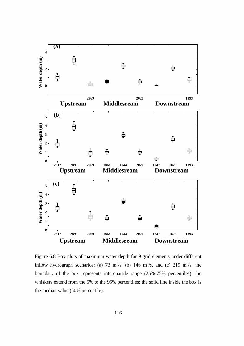
Figure 68 Box plots of maximum water depth for 9 grid elements under different
inflow hydrograph scenarios (a) 73 m3s (b) 146 m
3s and (c) 219 m
3s the
boundary of the box represents interquartile range (25-75 percentiles) the
whiskers extend from the 5 to the 95 percentiles the solid line inside the box is
the median value (50 percentile) 116
Figure 69 Box plots of maximum flow depth at different locations the box
represents interquartile range (25-75) the whiskers extend from the 5 to the
95 the solid line inside the box is identified as the median value (50) 118
XV
Figure 610 Box plots of maximum flow velocity in the channel at different
locations along the Buscot reach the box represents interquartile range (25-75
percentiles) the whiskers extend from the 5 to the 95 percentiles the solid line
inside the box is identified as the median value (50 percentile) 123
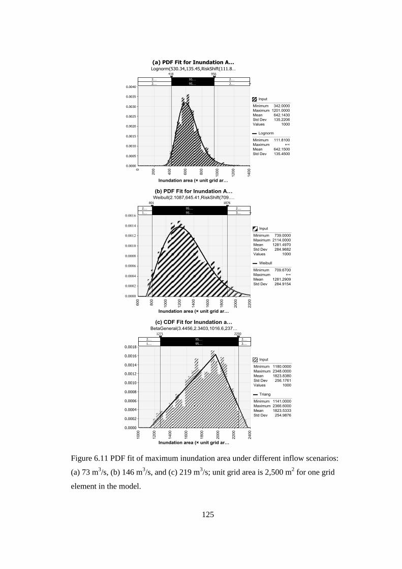
Figure 611 PDF fit of maximum inundation area under different inflow scenarios
(a) 73 m3s (b) 146 m
3s and (c) 219 m
3s unit grid area is 2500 m
2 for one grid
element in the model 125
Figure 71 three-dimensional (a) construction of collocation points by Smolyak‟s
sparse grid quadrature (k =5) and (b) construction of collocation points by
corresponding full tensor product quadrature 133
Figure 72 Integrated framework of combined GLUE and the DREAM sampling
scheme withwithout gPC approaches 135
Figure 73 Autocorrelations at lag z of different uncertain parameters of the MCMC
sampling chains within the GLUE inference 138
Figure 74 Two-dimensional posterior PDFs of the three uncertain parameters
predicted by the GLUE inference combined with DREAM sampling scheme with
10000 numerical executions Note nf is floodplain roughness nc is channel
roughness and lnkf represents logarithmic floodplain hydraulic conductivity 139
Figure 75 One-dimensional marginal probability density functions of three
uncertain parameters and their corresponding fitted PDFs Note three parameters
are floodplain roughness channel roughness and logarithmic hydraulic conductivity
(lnk) of floodplain 141
Figure 76 One-dimensional posterior PDFs of three uncertain parameters
conditioned on the observed inundation extent for the subjective threshold of 50
Note solid lines mean the exact posterior PDFs for the GLUE inference combined
with DREAM sampling (DREAM-GLUE) dotted and dash-dotted lines represent
the approximate posterior PDF for the DREAM-GLUE embedded with the 5th
- and
the 10th
-order gPC surrogate models 143
XVI
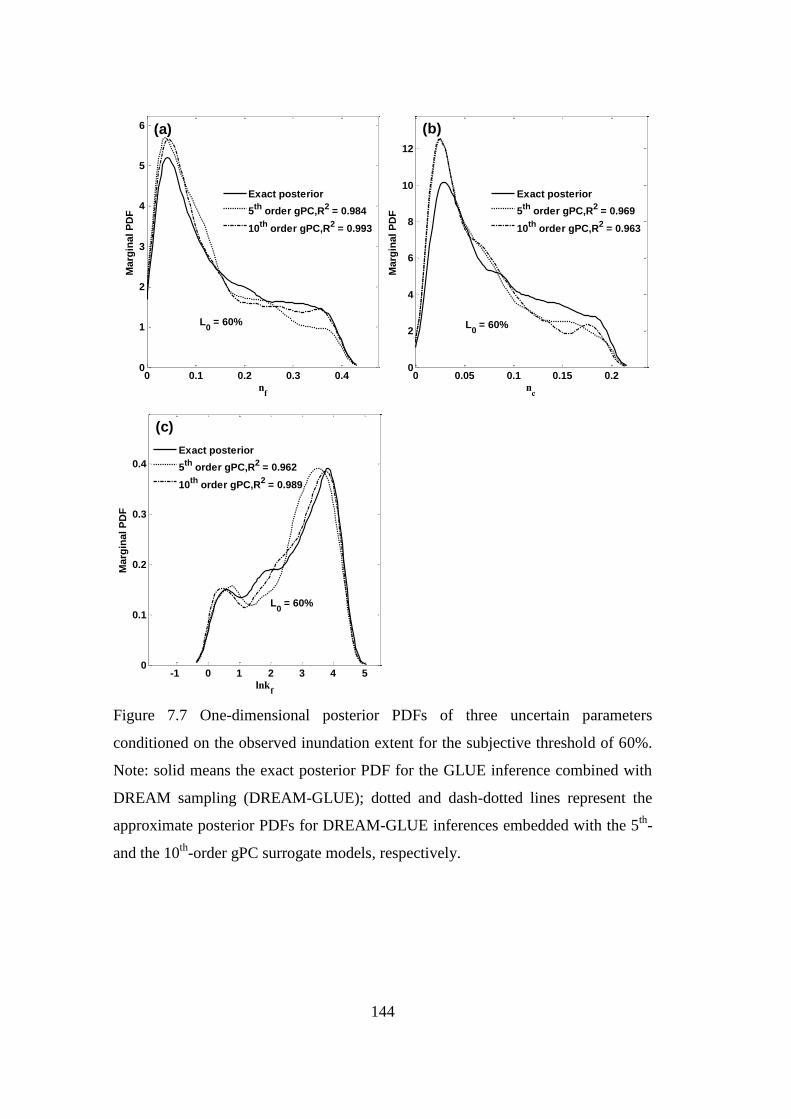
Figure 77 One-dimensional posterior PDFs of three uncertain parameters
conditioned on the observed inundation extent for the subjective threshold of 60
Note solid means the exact posterior PDF for the GLUE inference combined with
DREAM sampling (DREAM-GLUE) dotted and dash-dotted lines represent the
approximate posterior PDFs for DREAM-GLUE inferences embedded with the 5th
-
and the 10th
-order gPC surrogate models respectively 144
Figure 78 One-dimensional posterior PDFs of three uncertain parameters
conditioned on the observed inundation extent for the subjective threshold of 65
Note solid means the exact posterior PDF for GLUE inference combined with
DREAM sampling (DREAM-GLUE) dotted and dash-dotted lines represent the
approximate posterior PDF for DREAM-GLUE embedded with the 5th
- and the
10th
-order gPC surrogate models respectively 145
Figure 79 Autocorrelation at lag z of each uncertain parameter of the gPC-MCMC
sampling chains within the GLUE inference 146
Figure 710 One-dimensional posteriors of the three uncertain parameters and their
PDF fit for the subjectively level of 65 by gPC-DREAM-GLUE inference Note
posterior distributions of floodplain roughness and floodplain lnk (logarithmic
hydraulic conductivity) are obtained by the 10th
-order inference while posterior
distribution of channel roughness is by the 5th
-order one 148
XVII
LIST OF ABBREVIATIONS
BVP Boundary value problem
CDF
CP(s)
Cumulative Distribution Function
Collocation point(s)
DJPDF Discrete joint likelihood function
DREAM Differential Evolution Adaptive Metropolis
DREAM-GLUE GLUE inference coupled with DREAM sampling scheme
FP-KLE First-order perturbation method coupled with Karhunen-
Loevegrave expansion
FRM Flood risk management
GLUE Generalized likelihood uncertainty estimation
gPC Generalized polynomial chaos
gPC-DREAM DREAM sampling scheme coupled with gPC approach
gPC-DREAM-GLUE GLUE inference coupled with gPC-DREAM sampling
scheme
KLE Karhunen-Loevegrave expansion
LHS Latin Hyper Sampling
LF Likelihood function
MCS Monte Carlo simulation
PCM Probabilistic collocation method
XVIII
PCMKLE Probabilistic collocation method and Karhunen-Loevegrave
expansion
gPCKLE Generalized polynomial chaos (gPC) expansion and
Karhunen- Loevegrave expansion (gPCKLE)
PDF(s) Probability distribution function(s)
R2 Coefficient of determination
RMSE Root mean squared error
SNV(s) Standard normal variable(s)
SRSM(s) Stochastic response surface method(s)
SSG Smolyak sparse grid
1D One-dimensional
2D Two-dimensional
1D2D 1D coupled with 2D
XIX
SUMMARY
Flood inundation modelling is a fundamental tool for supporting flood risk
assessment and management However it is a complex process involving cascade
consideration of meteorological hydrological and hydraulic processes In order to
successfully track the flood-related processes different kinds of models including
stochastic rainfall rainfall-runoff and hydraulic models are widely employed
However a variety of uncertainties originated from model structures parameters
and inputs tend to make the simulation results diverge from the real flood situations
Traditional stochastic uncertainty-analysis methods are suffering from time-
consuming iterations of model runs based on parameter distributions It is thus
desired that uncertainties associated with flood modelling be more efficiently
quantified without much compromise of model accuracy This thesis is devoted to
developing a series of stochastic response surface methods (SRSMs) and coupled
approaches to address forward and inverse uncertainty-assessment problems in
flood inundation modelling
Flood forward problem is an important and fundamental issue in flood risk
assessment and management This study firstly investigated the application of a
spectral method namely Karhunen-Loevegrave expansion (KLE) to approximate one-
dimensional and two-dimensional coupled (1D2D) heterogeneous random field of
roughness Based on KLE first-order perturbation (FP-KLE) method was proposed
to explore the impact of uncertainty associated with floodplain roughness on a 2D
flooding modelling process The predicted results demonstrated that FP-KLE was
computationally efficient with less numerical executions and comparable accuracy
compared with conventional Monte Carlo simulation (MCS) and the decomposition
of heterogeneous random field of uncertain parameters by KLE was verified
Secondly another KLE-based approach was proposed to further tackle
heterogeneous random field by introducing probabilistic collocation method (PCM)
Within the framework of this combined forward uncertainty quantification approach
namely PCMKLE the output fields of the maximum flow depths were
approximated by the 2nd
-order PCM The study results indicated that the assumption
of a 1D2D random field of the uncertain parameter (ie roughness) could
XX
efficiently alleviate the burden of random dimensionality within the analysis
framework and the introduced method could significantly reduce repetitive
numerical simulations of the physical model as required in the traditional MCS
Thirdly a KLE-based approach for flood forward uncertainty quantification
namely pseudospectral collocation approach (ie gPCKLE) was proposed The
method combined the generalized polynomial chaos (gPC) with KLE To predict
the two-dimensional flood flow fields the anisotropic random input field
(logarithmic roughness) was approximated by the normalized KLE and the output
field of flood flow depth was represented by the gPC expansion whose coefficients
were obtained with a nodal set construction via Smolyak sparse grid quadrature
This study demonstrated that the gPCKLE approach could predict the statistics of
flood flow depth with less computational requirement than MCS it also
outperformed the PCMKLE approach in terms of fitting accuracy This study made
the first attempt to apply gPCKLE to flood inundation field and evaluated the
effects of key parameters on model performances
Flood inverse problems are another type of uncertainty assessment of flood
modeling and risk assessment The inverse issue arises when there is observed flood
data but limited information of model uncertain parameters To address such a
problem the generalized likelihood uncertainty estimation (GLUE) inferences are
introduced First of all an uncertainty analysis of the 2D numerical model called
FLO-2D embedded with GLUE inference was presented to estimate uncertainty in
flood forecasting An informal global likelihood function (ie F performance) was
chosen to evaluate the closeness between the simulated and observed flood
inundation extents The study results indicated that the uncertainty in channel
roughness floodplain hydraulic conductivity and floodplain roughness would
affect the model predictions The results under designed future scenarios further
demonstrated the spatial variability of the uncertainty propagation Overall the
study highlights that different types of information (eg statistics of input
parameters boundary conditions etc) could be obtained from mappings of model
uncertainty over limited observed inundation data
XXI
Finally the generalized polynomial chaos (gPC) approach and Differential
Evolution Adaptive Metropolis (DREAM) sampling scheme were introduced to
enhance the sampling efficiency of the conventional GLUE method By coupling
gPC with DREAM (gPC-DREAM) samples from high-probability region could be
generated directly without additional numerical executions if a suitable gPC
surrogate model of likelihood function was constructed in advance Three uncertain
parameters were tackled including floodplain roughness channel roughness and
floodplain hydraulic conductivity To address this inverse problem two GLUE
inferences with the 5th
and the 10th
gPC-DREAM sampling systems were
established which only required 751 numerical executions respectively Solutions
under three predefined subjective levels (ie 50 60 and 65) were provided by
these two inferences The predicted results indicated that the proposed inferences
could reproduce the posterior distributions of the parameters however this
uncertainty assessment did not require numerical executions during the process of
generating samples this normally were necessary for GLUE inference combined
with DREAM to provide the exact posterior solutions with 10000 numerical
executions
This research has made a valuable attempt to apply a series of collocation-based PC
approaches to tackle flood inundation problems and the potential of these methods
has been demonstrated The research also presents recommendations for future
development and improvement of these uncertainty approaches which can be
applicable for many other hydrologicalhydraulics areas that require repetitive runs
of numerical models during uncertainty assessment and even more complicated
scenarios
1
CHAPTER 1 INTRODUCTION
11 Floods and role of flood inundation modelling
Flooding has always been a major concern for many countries as it causes
immeasurable human loss economic damage and social disturbances (Milly et al
2002 Adger et al 2005) In urban areas flooding can cause significant runoff and
destroy traffic system public infrastructure and pathogen transmission in drinking
water in other areas it could also ruin agricultural farm lands and bring
interference to the fish spawning activities and pollute (or completely destroy) other
wildlife habitats Due to impact of possible climate change the current situation
may become even worse To tackle such a problem many types of prevention or
control measures are proposed and implemented With an extensive historic survey
on hydrogeology topography land use and public infrastructure for a flooding area
the hydrologicalhydraulic engineers and researchers can set up conceptual physical
model andor mathematical models to represent flood-related processes and give
predictions for the future scenarios (Pender and Faulkner 2011)
Among various alternatives within the framework of flood risk management (FRM)
flood inundation model is considered as one of the major tools in (i) reproducing
historical flooding events (including flooding extent water depth flow peak
discharge and flow velocity etc) and (ii) providing predictions for future flooding
events under specific conditions According to the simulation results from flood
modelling decision-makers could conduct relevant risk assessment to facilitate the
design of cost-effective control measures considering the impacts on receptors
such as people and their properties industries and infrastructure (Pender and
Faulkner 2011)
12 Flood inundation modelling under uncertainty
Due to the inherent complexity of flood inundation model itself a large number of
parameters involved and errors associated with input data or boundary conditions
there are always uncertainties affecting the accuracy validity and applicability of
2
the model outputs which lead to (Pappenberger et al 2008 Pender and Faulkner
2011 Altarejos-Garciacutea et al 2012)
(1) Errors caused by poorly defined boundary conditions
(2) Errors caused by measurements done in model calibration and benchmarking
(3) Errors caused by incorrect definition of model structures
(4) Errors caused by operational and natural existence of unpredictable factors
Such errors may pose significant impact on flood prediction results and result in
biased (or even false) assessment on the related damages or adverse consequences
which unavoidably would increase the risk of insufficient concern from flood
managers or the waste of resources in flood control investment (Balzter 2000
Pappenberger et al 2005 Pappenberger et al 2008 Peintinger et al 2007 Beven
and Hall 2014) Therefore a necessary part of food risk assessment is to conduct
efficient uncertainty quantification and examine the implications from these
uncertainties Furthermore to build up an efficient and accurate model in providing
reliable predictions Beven and Binley (1992) suggested that a unique optimum
model that would give the most efficient and accurate simulation results was almost
impossible and a set of goodness-of-fit combinations of the values of different
parameters or variables would be acceptable in comparing with the observed data
How to establish an appropriate framework for uncertainty analysis of flood
modelling is receiving more and more attentions
From literature review (as discussed in Chapter 2) there are still a number of
limitations that challenge the development of uncertainty analysis tools for flood
inundation modelling The primary limitation is that performing uncertainty
analysis generally involves repetitive runs of numerical models (ie flood
inundation models in this study) which normally requires expensive computational
resources Furthermore due to distributed nature of geological formation and land
use condition as well as a lack of sufficient investigation in obtaining enough
information some parameters are presented as random fields associated with
physical locations such as Manning‟s roughness and hydraulic conductivity (Roy
3
and Grilli 1997 Simonovic 2009 Grimaldi et al 2013 Beven and Hall 2014 Yu
et al 2015) However in the field of flood inundation modelling such uncertain
parameters are usually assumed as homogeneous for specific types of domains (eg
grassland farms forest and developed urban areas) rather than heterogeneous
fields this could lead to inaccurate representation of the input parameter fields
(Balzter 2000 Peintinger et al 2007 Altarejos-Garciacutea et al 2012 Beven and
Hall 2014 Westoby et al 2015) Misunderstanding of these parameters would
ultimately lead to predictions divergent from the real flood situations Finally it is
normally encountered that some parameters have little or even no information but
the measurement data (like the observation of water depths at different locations)
may be available Then it is desired to use inverse parameter evaluation (ie
Bayesian approach) to obtain the real or true probability distributions of the input
random fields In flooding modelling process the related studies are still limited
(Balzter 2000 Peintinger et al 2007 Altarejos-Garciacutea et al 2012 Beven and
Hall 2014 Yu et al 2015)
13 Objectives and scopes
The primary objective of this thesis is the development of computationally-efficient
approaches for quantifying uncertainties originated from the spatial variability
existing in parameters and examining their impacts on flood predictions through
numerical models The study focuses on the perspectives of (i) alleviation of
computational burden due to the assumption of spatial variability (ii) practicability
of incorporating these methods into the uncertainty analysis framework of flood
inundation modelling and (iii) ease of usage for flood risk managers Another
objective of this thesis is to embed these efficient approaches into the procedure of
flood uncertainty assessment such as the informal Bayesian inverse approach and
significantly improve its efficiency In detail the scopes of this study are
(1) To develop a first-order perturbation method based on first order perturbation
method and Karhunen-Loevegrave expansion (FP-KLE) Floodplain roughness over a 2-
dimensional domain is assumed a statistically heterogeneous field with lognormal
distributions KLE will be used to decompose the random field of log-transferred
4
floodplain roughness and the maximum flow depths will be expanded by the first-
order perturbation method by using the same set of random variables as used in the
KLE decomposition Then a flood inundation model named FLO-2D will be
adopted to numerically solve the corresponding perturbation expansions
(2) To introduce an uncertainty assessment framework based on Karhunen-Loevegrave
expansion (KLE) and probabilistic collocation method (PCM) to deal with flood
inundation modelling under uncertainty The Manning‟s roughness coefficients for
channel and floodplain are treated as 1D and 2D respectively and decomposed by
KLE The maximum flow depths are decomposed by the 2nd
-order PCM
(3) To apply an efficient framework of pseudospectral collocation approach
combined with generalized polynomial chaos (gPC) and Karhunen-Loevegrave
expansion and then examine the flood flow fields within a two-dimensional flood
modelling system In the proposed framework the heterogeneous random input
field (logarithmic Manning‟s roughness) will be approximated by the normalized
KLE and the output field of flood flow depth will be represented by the gPC
expansion whose coefficients will be obtained with a nodal set construction via
Smolyak sparse grid quadrature
(4) To deal with flood inundation inverse problems within a two-dimensional FLO-
2D model by an informal Bayesian method generalized likelihood uncertainty
estimation (GLUE) The focuses of this study are (i) investigation of the uncertainty
arising from multiple variables in flood inundation mapping using Monte Carlo
simulations and GLUE and (ii) prediction of the potential inundation maps for
future scenarios The study will highlight the different types of information that
may be obtained from mappings of model uncertainty over limited observed
inundation data and the efficiency of GLUE will be demonstrated accordingly
(5) To develop an efficient framework for generalized likelihood uncertainty
estimation solution (GLUE) for flood inundation inverse problems The framework
is an improved version of GLUE by introducing Differential Evolution Adaptive
Metropolis (DREAM) sampling scheme and generalized polynomial chaos (gPC)
surrogate model With such a framework samples from high-probability region can
5
be generated directly without additional numerical executions if a suitable gPC
surrogate model has been established
14 Outline of the thesis
Figure 11 shows the structure of this thesis Chapter 1 briefly presents the
background of flood inundation modelling under uncertainty In Chapter 2 a
literature review is given focusing on (i) three types of numerical models including
one-dimensional (1D) two-dimensional (2D) and 1D coupled with 2D (1D2D)
and their representatives (ii) general classification of uncertainties and explanations
about uncertainties of boundary value problems (BVP) with a given statistical
distribution in space and time such as floodplain roughness and hydraulic
conductivity (iii) conventional methodologies of analyzing uncertainty in the flood
modelling process including forward uncertainty propagation and inverse
uncertainty quantification
Chapter 3 presents the application of Karhunen-Loevegrave expansion (KLE)
decomposition to the random field of floodplain roughness (keeping the channel
roughness fixed) within a coupled 1D (for channel flow) and 2D (for floodplain
flow) physical flood inundation model (ie FLO-2D) The method is effective in
alleviating computational efforts without compromising the accuracy of uncertainty
assessment presenting a novel framework using FLO-2D
Chapters 4 and 5 present two integral frameworks by coupling the stochastic surface
response model (SRSM) with KLE to tackle flood modelling problems involving
multiple random input fields under different scenarios In Chapter 4 an uncertainty
assessment framework based on KLE and probabilistic collocation method (PCM)
is introduced to deal with the flood inundation modelling under uncertainty The
roughness of the channel and floodplain are assumed as 1D and 2D random fields
respectively the hydraulic conductivity of flood plain is considered as a 2D random
field KLE is used to decompose the input fields and PCM is used to represent the
output fields Five testing scenarios with different combinations of inputs and
parameters based on a simplified flood inundation case are examined to
demonstrate the methodology‟s applicability
6
In Chapter 5 another efficient framework of pseudospectral collocation approach
combined with the generalized polynomial chaos (gPC) expansion and Karhunen-
Loevegrave expansion (gPCKLE) is applied to study the nonlinear flow field within a
two-dimensional flood modelling system Within this system there exists an
anisotropic normal random field of logarithmic roughness (Z) whose spatial
variability would introduce uncertainty in prediction of the flood flow field In the
proposed framework the random input field of Z is approximated by normalized
KLE and the output field of flood flow is represented by the gPC expansion For
methodology demonstration three scenarios with different spatial variability of Z
are designed and the gPC models with different levels of complexity are built up
Stochastic results of MCS are provided as the benchmark
Chapters 6 and 7 are studies of flood inverse problems where the information for
the input parameters of the modelling system is insufficient (even none) but
measurement data can be provided from the historical flood event In Chapter 6 we
attempt to investigate the uncertainty arising from multiple parameters in FLO-2D
modelling using an informal Bayesian approach namely generalized likelihood
uncertainty estimation (GLUE) According to sensitivity analysis the roughness of
floodplain the roughness of river channel and hydraulic conductivity of the
floodplain are chosen as uncertain parameters for GLUE analysis In Chapter 7 an
efficient MCMC sampling-based GLUE framework based on the gPC approach is
proposed to deal with the inverse problems in the flood inundation modeling The
gPC method is used to build up a surrogate model for the logarithmic LF so that the
traditional implementation of GLUE inference could be accelerated
Chapter 8 summarizes the research findings from the thesis and provides
recommendations for future works
7
Flood inverse uncertainty quantificationFlood forward uncertainty propagation
Chaper 1 Introduction
Floods and flood inundation modelling
Flood inundation modelling under uncertainty and its limitations
Objectives and scopes
Outline of the thesis
Chaper 2 Literature Review
Flood and flood damage
Flood inundation models
Uncertainty in flood modelling
Probabilistic theory for flood uncertainty quantification
Approaches for forward uncertainty propagation
Approaches for inverse uncertainty quantification
Challenges in flood inundation modelling under uncertainty
Chaper 7 gPC-based generalized likelihood
uncertainty estimation inference for flood inverse
problems
Collocation-based gPC approximation of
likelihood function
Application of gPC-DREAM sampling scheme in
GLUE inference for flood inverse problems
Case study of the River Thames UK
Summary
Chaper 3 Uncertainty analysis for flood
inundation modelling with a random floodplain
roughness field
Karhunen-Loevegrave expansion decomposition to the
random field of floodplain roughness coefficients
Case description of the River Thames UK
Results and discussion
Chaper 6 Assessing uncertainty propagation in
FLO-2D using generalized likelihood uncertainty
estimation
Sensitivity analysis
generalized likelihood uncertainty estimation
(GLUE) framework
Scenarios analysis of the River Thames UK
Conclusions
Chaper 4 Uncertainty Assessment of Flood
Inundation Modelling with a 1D2D Random
Field
KLE decomposition of 1D2D of Manningrsquos
roughness random field PCMKLE in flood inundation modelling
Results analysis
Chaper 5 Efficient pseudospectral approach for
inundation modelling
process with an anisotropic random input field
gPCKLE is applied to study the nonlinear flow
field within a two-dimensional flood modelling
system
Illustrative example
Conclusions
Chaper 8 Conclusions
Conclusions and recommendations
Figure 11 Outline of the thesis
8
CHAPTER 2 LITERATURE REVIEW
21 Introduction
Flood control is an important issue worldwide With the rapid technological and
scientific development flood damage could somewhat be mitigated by modern
engineering approaches However the severity and frequency of flood events have
seen an increasing trend over the past decades due to potential climate change
impacts and urbanization Mathematical modelling techniques like flood inundation
modelling and risk assessment are useful tools to help understand the flooding
processes evaluate the related consequences and adopt cost-effective flood control
strategies However one major concern is that food like all kinds of hazards is no
exception uncertain essentially Deviation in understanding the input (or input range)
and modelling procedure can bring about uncertainty in the flood prediction This
could lead to (1) under-preparation and consequently huge loss caused by
avoidable flood catastrophe 2) over-preparation superfluous cost and labour force
and as a result loss of credibility from public to government (Smith and Ward
1998 Beven and Hall 2014) The involvement of uncertainty assessment in a flood
model requires quantitative evaluation of the propagation of different sources of
uncertainty This chapter reviews the recent major flood damage events occurred
around the word the structures of flood hydraulic models and the uncertainty
estimation during the flood risk assessment and mitigation management
22 Flood and flood damage
Flood is water in the river (or other water body) overflowing river bank and cover
the normally dry land (Smith and Ward 1998 Beven and Hall 2014) Most of
flood events are the natural product and disasters Flood can cause damage to (i)
human‟s lives (ii) governmental commercial and educational buildings (iii)
infrastructure structures including bridges drainage systems and roadway and
subway (iv) agriculture forestry and animal husbandry and (v) the long-term
environmental health
9
In southeast Asia a series of separate flood events in the 2011 monsoon season
landed at Indochina and then across other countries including Thailand Cambodia
Myanmar Laos and especially Vietnam Until the end of the October in 2011 about
23 million lives have been affected by the catastrophe happened in the country of
Thailand (Pundit-Bangkok 2011) Meanwhile another flood disaster occurred at
the same time hit nearly more than a million people in Cambodia according to the
estimation by the United Nations Since August 2011 over 2800 people have been
killed by a series of flooding events caused by various flooding origins in the above
mentioned Southeast Asian countries (Sakada 2011 Sanguanpong 2011) In July
2012 Beijing the capital of China suffered from the heaviest rainfall event during
the past six decades During this process of flooding by heavy rainfall more than
eight hundred thousand people were impacted by a series of severe floods in the
area and 77 people lost their lives in this once-in-sixty-year flooding The
floodwater covered 5000 hectares of farmland and a large amount of farm animals
were killed causing a huge economic loss of about $955 million (Whiteman 2012)
The damage to environment is also imponderable (Taylor et al 2013)
Other parts of the world also faced serious flood issues During the second quarter
in 2010 a devastating series of flood events landed on several Central European and
many others countries including Germany Hungary Austria Slovakia Czech
Republic Serbia Ukraine at least 37 people lost their lives during the flooding
events and up to 23000 people were forced to leave their home in this disaster The
estimated economic cost was nearly 25 million euros (euronews 2010 Matthew
2010) In USA a 1000-year flood in May 2010 attacked Tennessee Kentucky and
north part of Mississippi areas in the United States and resulted in a large amount
of deaths and widespread economic damages (Marcum 2010)
From the above-mentioned events in the world flood is deemed a big hindrance to
our social lives and economic development Flood risk assessment and management
is essential to help evaluate the potential consequences design cost-effective
mitigation strategies and keep humanity and the society in a healthy and
sustainable development
10
23 Flood inundation models
For emergency management the demand for prediction of disastrous flood events
under various future scenarios (eg return periods) is escalating (Middelkoop et al
2004 Ashley et al 2005 Hall et al 2005 Hunter et al 2007) Due to absence of
sufficient historical flood records and hydrometric data numerical models have
become a gradually attractive solution for future flood predictions (Hunter et al
2007 Van Steenbergen 2012) With the advancement of remote-sensing
technology and computational capability significant improvement has been made in
flood inundation modelling over the past decades The understanding of hydraulics
processes that control the runoff and flood wave propagation in the flood modelling
has become clearer with the aids from numerical techniques high computational
capability sophisticated calibration and analysis methods for model uncertainty
and availability of new data sources (Franks et al 1998 Jakeman et al 2010
Pender and Faulkner 2011) However undertaking large-scale and high-resolution
hydrodynamic modelling for the complicated systems of river and floodplain and
carrying out flood risk assessment at relatively fine tempo-spatial scales (eg
Singapore) is still challenging The goal of using and developing flood models
should be based on consideration of multiple factors such as (i) the computational
cost for the numerical executions of hydrodynamic models (ii) investment in
collection of information for input parameters (iii) model initialization and (iv) the
demands from the end-users (Beven 2001 Johnson et al 2007a)
According to dimensional representation of the flood physical process or the way
they integrate different dimensional processes flood inundation models can
generally be categorized into 1-dimensional (1D) 2-dimensional (2D) and three-
dimensional (3D) From many previous studies it is believed that 3D flood models
are unnecessarily complex for many scales of mixed channel and floodplain flows
and 2D shallow water approximation is generally in a sufficient accuracy (Le et al
2007 Talapatra and Katz 2013 Warsta et al 2013 Work et al 2013 Xing et al
2013) For abovementioned causes dynamically fluctuating flows in compound
channels (ie flows in channel and floodplain) have been predominantly handled by
11
1D and 2D flood models (Beffa and Connell 2001 Connell et al 2001) Table 21
shows a classification of major flood inundation models
Table 21 Classification of flood inundation models (adapted from Pender and
Faulkner 2011)
Model Description Applicable
scales Computation Outputs
Typical
Models
1D
Solution of the
1D
St-Venant
equations
[10 1000]
km Minutes
Water depth
averaged
cross-section
velocity and
discharge at
each cross-
section
inundation
extent
ISIS MIKE
11
HEC-RAS
InfoWorks
RS
1D+
1D models
combined with
a storage cell
model to the
modelling of
floodplain flow
[10 1000]
km Minutes
As for 1d
models plus
water levels
and inundation
extent in
floodplain
storage cells
ISIS MIKE
11
HEC-RAS
InfoWorks
RS
2D 2D shallow
water equations
Up to 10000
km
Hours or
days
Inundation
extent water
depth and
depth-
averaged
velocities
FLO-2D
MIKE21
SOBEK
2D-
2D model
without the
momentum
conservation
for the
floodplain flow
Broad-scale
modelling for
inertial effects
are not
important
Hours
Inundation
extent water
depth
LISFLOOD-
FP
3D
3D Rynolds
averaged
Navier-Stokes
equation
Local
predictions of
the 3D
velocity fields
in main
channels and
floodplains
Days
Inundation
extent
water depth
3D velocities
CFX
Note 1D+ flood models are generally dependant on catchment sizes it also has the
capacity of modelling the large-scale flood scenarios with sparse cross-section data (Pender
and Faulkner 2011)
12
Another kind of hydraulic models frequently implemented to flood inundation
prediction is namely coupled 1D and 2D (1D2D) models Such kind of models
regularly treat in-channel flow(s) with the 1D Saint-Venant equations while
treating floodplain flows using either the full 2D shallow water equations or storage
cells linked to a fixed grid via uniform flow formulae (Beven and Hall 2014) Such
a treatment satisfies the demand of a very fine spatial resolution to construct
accurate channel geometry and then an appreciable reduction is achieved in
computational requirement
FLO-2D is a physical process model that routes rainfall-runoff and flood
hydrographs over unconfined flow surfaces or in channels using the dynamic wave
approximation to the momentum equation (Obrien et al 1993 FLO-2D Software
2012) It has been widely used as an effective tool for delineating flood hazard
regulating floodplain zoning or designing flood mitigation The model can simulate
river overbank flows and can be used on unconventional flooding problems such as
unconfined flows over complex alluvial fan topography and roughness split
channel flows muddebris flows and urban flooding FLO-2D is on the United
States Federal Emergency Management Agency (FEMA)‟s approval list of
hydraulic models for both riverine and unconfined alluvial fan flood studies (FLO-
2D Software 2012)
As a representative of 1D2D flood inundation models FLO-2D is based on a full
2D shallow-water equation (Obrien et al 1993 FLO-2D Software 2012)
h
hV It
(21a)
1 1
f o
VS S h V V
g g t
(21b)
where h is the flow depth V represents the averaged-in-depth velocity in each
direction t is the time So is the bed slope and Sf is the friction slope and I is lateral
flow into the channel from other sources Equation (21a) is the continuity equation
or mass conservation equation and Equation (21b) is the momentum equation
both of them are the fundamental equations in the flood modelling Equation (21a)
13
and (21b) are solved on a numerical grid of square cells through which the
hydrograph is routed propagating the surface flow along the eight cardinal
directions In FLO-2D modelling system channel flow is 1D with the channel
geometry represented by either rectangular or trapezoidal cross sections and
meanwhile the overland flow is modelled 2D as either sheet flow or flow in
multiple channels (rills and gullies) If the channel capacity is exceeded the
overbanking flow in channel will be calculated subsequently Besides the change
flow between channel and floodplain can be computed by an interface routine
(FLO-2D Software 2012)
24 Uncertainty in flood modelling
Due to the inherent complexity of the flood model itself a large number of
parameters involved and errors associated with input data or boundary conditions
there are always uncertainties that could cause serious impact on the accuracy
validity and applicability of the flood model outputs (Pappenberger et al 2005
Pappenberger et al 2008 Romanowicz et al 2008 Blazkova and Beven 2009
Pender and Faulkner 2011 Altarejos-Garciacutea et al 2012) The sources of the
uncertainties in the modelling process can be defined as the causes that lead to
uncertainty in the forecasting process of a system that is modelled (Ross 2010) In
the context of flood inundation modelling major sources of uncertainty can be
summarized as (Beven and Hall 2014)
1) Physical structural uncertainty uncertainties are introduced into modelling
process by all kinds of assumptions for basic numerical equations model
establishment and necessary simplifications assisting in the physical assumptions
for the real situation or system
2) Model input uncertainty imprecise data to configure boundary and initial
conditions friction-related parameters topographical settings and details of the
hydraulic structures present along the river or reach component
3) Parameter uncertainty incorrectinsufficient evaluation or quantification of
model parameters cause magnitude of the parameters being less or more than the
14
acceptable values
4) Operational and natural uncertainty existence of unpredictable factors (such
as dam breaking glacier lake overflowing and landsliding) which make the model
simulations deviate from real values
25 Probabilistic theory for flood uncertainty quantification
How to identify uncertainty and quantify the degree of uncertainty propagation has
become a major research topic over the past decades (Beven and Binley 1992
Beven 2001 Hall and Solomatine 2008) Over the past decades the theory of
probability has been proposed and proven as a predominant approach for
identification and quantification of uncertainty (Ross 2010) Conceptually
probability is measured by the likelihood of occurrence for subsets of a universal
set of events probability density function (PDF) is taken to measure the probability
of each event and a number of PDFs values between 0 and 1 are assigned to the
event sets (Ayyub and Gupta 1994) Random variables stochastic processes
and events are generally in the centre of probabilistic theory and mathematical
descriptions or measured quantities of flood events that may either be single
occurrences or evolve in history in an apparently random way In probability theory
uncertainty can be identified or quantified by (i) a PDF fX (x) in which X is defined
as the uncertain variable with its value x and (ii) cumulative distribution function
(CDF) can be named as XP x in which the probability of X in the interval (a b] is
given by (Hill 1976)
(22)
Uncertainty quantification is implemented to tackle two types of problems involved
in the stochastic flood modelling process including forward uncertainty
propagation and inverse uncertainty quantification shown in Fig 22 The former
method is to quantify the forward propagation of uncertainty from various sources
of random (uncertain) inputs These sources would have joint influence on the flood
i n u n d a t i o n
P a lt X lt b( ) = fXx( )ograve dx
15
Figure 21 Illustration of (a) Probability Density Function (PDF) and (b)
Cumulative Distribution Function (CDF)
Figure 22 Schematic diagram of uncertainty quantification for stochastic
inundation modelling
outputs such as flood depth flow velocity and inundation extent The latter one is
to estimate model uncertainty and parameter uncertainty (ie inverse problem) that
need to be calibrated (assessed) simultaneously using historical flood event data
Previously a large number of studies were conducted to address the forward
uncertainty problems and diversified methodologies were developed (Balzter 2000
Pappenberger et al 2008 Peintinger et al 2007 Beven and Hall 2014 Fu et al
2015 Jung and Merwade 2015) Meanwhile more and more concerns have been
(a) PDF Probability distribution function
x
f(x
)
x
P(x
)
(b) PDF Cumulative distribution function
Forward uncertainty propagation
Inverse uncertainty quantification
Predictive Outputs
(ie flood depth
flow velocity and
inundation extent)
Calibration with
historical flood
event(s)
Parameter PDF
updaterestimator
Flood
inundation
model (ie
FLO-2D)
Parameters
with the
PDFs
Statistics of
the outputs
16
put on the inverse problems especially for conditions where a robust predictive
system is strongly sensitive to some parameters with little information being known
before-hand Subsequently it is crucial to do sensitive analysis for these parameters
before reliable predictions are undertaken to support further FRM
26 Approaches for forward uncertainty propagation
When we obtain the PDF(s) of the uncertainty parameter(s) through various ways
such as different scales of in-situ field measurements and experimental studies
uncertainty propagation is applied to quantify the influence of uncertain input(s) on
model outputs Herein forward uncertainty propagation aims to
1) To predict the statistics (ie mean and standard deviation) of the output for
future flood scenarios
2) To assess the joint PDF of the output random field Sometimes the PDF of
the output is complicated and low-order moments are insufficient to describe it In
such circumstances a full joint PDF is required for some optimization framework
even if the full PDF is in high-computational cost
3) To evaluate the robustness of a flood numerical model or other mathematical
model It is useful particularly when the model is calibrated using historical events
and meant to predict for future scenarios
Probability-based approaches are well-developed and can be classified into
sampling-based approaches (eg MCS) and approximation (nonsampling-based)
approaches (eg PCM)
261 Monte Carlo Simulation (MCS)
The Monte Carlo simulation as the most commonly used approach based on
sampling can provide solutions to stochastic differential equations (eg 2D shallow
water equations) in a straightforward and easy-to-implement manner (Ballio and
Guadagnini 2004) Generally for the flood modelling process its general scheme
consists of four main procedures (Saltelli et al 2000 Saltelli 2008)
17
(1) Choose model uncertain parameters (ie random variables) which are usually
sensitive to the model outputs of interest
(2) Obtain PDFs for the selected random variables based on the previous
experience and knowledge or in-situ fieldlab measurements
(3) Carry out sampling (eg purely random sampling or Latin Hypercube sampling)
based on the PDFs of the random variables solve the corresponding flood
numerical models (eg 2D shallow water equations) and abstract the outputs from
the simulation results
(4) Post-process the statistics of model outputs and conduct further result analysis
It is should be noted that the 3rd
procedure of MCS is described for full-uncorrelated
random variables and the input samples are generated independently based on their
corresponding PDFs This assumption is taken throughout the entire thesis when
involving MCS
There are many world-wide applications of MCS in the area of flood inundation
modelling and risk analysis including prediction of floodplain flow processes
validation of inundation models and sensitivity analysis of effective parameters
(Kuczera and Parent 1998 Kalyanapu et al 2012 Yu et al 2013 Beven and Hall
2014 Loveridge and Rahman 2014) For instance Hall et al (2005) applied a
MCS-based global sensitivity analysis framework so-called bdquoSobol‟ method to
quantify the uncertainty associated with the channel roughness MCS was applied to
reproduce the probability of inundation of the city Rome for a significant flood
event occurred in 1937 in which the processes of rainfall rainfall-runoff river
flood propagation and street flooding were integrated into a framework of forward
uncertainty propagation to produce the inundation scenarios (Natale and Savi 2007)
Yu et al (2013) developed a joint MC-FPS approach where MCS was used to
evaluate uncertainties linked with parameters within the flood inundation modelling
process and fuzzy vertex analysis was implemented to promulgate human-induced
uncertainty in flood risk assessment Other latest applications of MCS to address
stochastic flood modelling system involving multi-source uncertainty
18
abovementioned in section 24 such as construction of believable flood inundation
maps predictions of the PDFs of acceptable models for specific scenarios assist to
identification of parametric information investigation of robustness and efficiency
of proposed improved (or combined) methodologies and etc (Mendoza et al 2012
Fu and Kapelan 2013 Rahman et al 2013 Mohammadpour et al 2014
OConnell and ODonnell 2014 Panjalizadeh et al 2014 Salinas et al 2014
Yazdi et al 2014 Jung and Merwade 2015 Yu et al 2015)
However the main drawback of MCS and MCS-based methods is to obtain
convergent stochastic results for flood forward uncertainty propagation a relatively
large amount of numerical simulations for this conventional method is required
especially for real-world flood applications which could bring a fairly high
computational cost (Pender and Faulkner 2011)
262 Response surface method (RSM)
As an alternative to MCS response surface method (RSM) attempts to build an
optimal surface (ie relationship) between the explanatory variables (ie uncertain
inputs) and the response or output variable(s) of interest on the basis of simulation
results or designed experiments (Box and Draper 2007) SRM is only an
approximation where its major advantage is the easiness in estimation and usage It
can provide in-depth information even when limited data is available with the
physical process besides it needs only a small number of experiments to build up
the interaction or relationship of the independent variables on the response (Box et
al 1978 Box and Draper 2007) Assume variable vector x is defined as the
combination of (x1 x 2hellip xk) of which each is generated according to its
corresponding PDF and f has a functional relationship as y = f(x) Figure 22 shows
a schematic demonstration of response surface method (RSM) for two-dimensional
forward uncertainty propagation Herein RSM provides a statistical way to explore
the impact from two explanatory variables x1 and x2 on the response variable of
interest (ie a response surface y) It can be seen that each point of the response
surface y have one-to-one response to each point of x(x1 x2) Herein x1 and x2 have
independent PDFs respectively
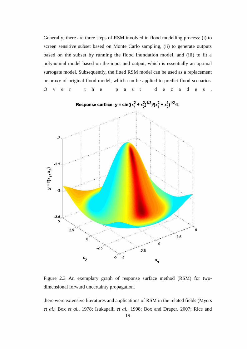
19
Generally there are three steps of RSM involved in flood modelling process (i) to
screen sensitive subset based on Monte Carlo sampling (ii) to generate outputs
based on the subset by running the flood inundation model and (iii) to fit a
polynomial model based on the input and output which is essentially an optimal
surrogate model Subsequently the fitted RSM model can be used as a replacement
or proxy of original flood model which can be applied to predict flood scenarios
O v e r t h e p a s t d e c a d e s
Figure 23 An exemplary graph of response surface method (RSM) for two-
dimensional forward uncertainty propagation
there were extensive literatures and applications of RSM in the related fields (Myers
et al Box et al 1978 Isukapalli et al 1998 Box and Draper 2007 Rice and
20
Polanco 2012) For instance Rice and Polanco (2012) built up a response surface
that defined the relationship between the variables (ie soil properties and
subsurface geometry) and the factor of safety (ie unsatisfactory performance) and
used it as a surrogate model to simulate the output in replace of the initial
complicated and high-nonlinearity erosion process for a given river flood level
However as the input variables of RSM are generated from random sampling the
method also faces the same challenge of requiring a large amount of numerical
simulations as traditional MCS In addition traditional response surface by RSM
sometimes may be divergent due to its construction with random samples (Box et
al 1978)
263 Stochastic response surface method (SRSM)
As an extension to classic RSM stochastic response surface method (SRSM) has a
major difference in that the former one is using random variables to establish the
relationship between the inputs and outputs (ie response surface) and the latter one
make use of deterministic variables as input samples By using deterministic
variables SRSM can obtain less corresponding input samples to build up the
response surface (ie relationship) between the input(s) and the output(s) and is
relatively easier to implement
General steps of SRSM approximation can be summarized into (i) representation of
random inputs (eg floodplain roughness coefficient) (ii) approximation of the
model outputs (eg flood flow depth) (iii) computation of the moments (eg mean
and standard deviation) of the predicted outputs and (iv) assessment of the
efficiency and accuracy of the established surrogate model (ie SRSM)
Polynomial Chaos Expansion (PCE) approach
To tackle the computational problem of MCS-based methods polynomial chaos
expansion (PCE) approximation as one of the types of SRSM was firstly proposed
by Wiener (1938) and has been applied in structure mechanics groundwater
modelling and many other fields (Isukapalli et al 1998 Xiu and Karniadakis
21
2002) It is used to decompose the random fields of the output y(x) as follows
(Ghanem and Spanos 1991)
Γ
Γ
Γ
1 1
1
1
i i 1 21 2
1 2
1 2
i i i 1 2 31 2 3
1 2 3
0 i 1 i
i
i
2 i i
i i
i i
3 i i i
i i i
y ω a a ς ω
a ς ω ς ω
a ς ω ς ω ς ω
=1
=1 =1
=1 =1 =1
(23)
where event ω (a probabilistic space) a0 and1 2 di i ia represent the deterministic
PCE coefficients Γ1 dd i iς ς
are defined as a set of d-order orthogonal polynomial
chaos for the random variables 1 di iς ς Furthermore if
1 di iς ς can be
assumed as NRVs generated from independent standard normal distributions
Γ1 dd i iς ς becomes a d-order Q-dimensional Hermite Polynomial (Wiener 1938)
ΓT T
1 d
1 d
1 1dd
2 2d i i
i i
ς ς 1 e eς ς
ς ς
(24)
where ς represents a vector of SNVs defined as 1 d
T
i iς ς The Hermite
polynomials can be used to build up the best orthogonal basis for ς and then help
construct the random field of output (Ghanem and Spanos 1991) Equation (23)
can be approximated as (Zheng et al 2011)
P
i i
i
y c φ=1
$ (25)
where ci are the deterministic PCE coefficients including a0 and1 2 di i ia φi(ς) are the
Hermite polynomials in Equation (23) In this study the number of SNVs is
required as Q and therefore the total number of the items (P) can be calculated as P
= (d + Q)(dQ) For example the 2nd
-order PCE approximation of y can be
expressed as (Zheng et al 2011)
22
ij
Q Q Q 1 Q2
0 i i ii i i j
i i i j i
y a a a 1 a
=1 =1 =1
$ (26)
where Q is the number of the SNVs
Generally PCE-based approach can be divided into two types intrusive Galerkin
scheme and uninstructive Probabilistic Collocation Method (PCM) Ghanem and
Spanos (1991) utilized the Galerkin projection to establish so-called spectral
stochastic finite element method (SSFEM) which was applied to provide suitable
solutions of stochastic complex modelling processes However Galerkin projection
as one of the key and complicated procedures of the traditional PCE-based approach
produces a large set of coupled equations and the related computational requirement
would rise significantly when the numbers of random inputs or PCE order increases
Furthermore the Galerkin scheme requires a significant modification to the existing
deterministic numerical model codes and in most cases these numerical codes are
inaccessible to researchers For stochastic flood inundation modelling there are
many well-developed commercial software packages or solvers for dealing with
complex real-world problems they are generally difficult to apply the Galerkin
scheme
Later on the Probabilistic Collocation Method (PCM) as a computationally
efficient technique was introduced to carry out uncertainty analysis of numerical
geophysical models involving multi-input random field (Webster 1996 Tatang et
al 1997) Comparing with Galerkin-based PCE approach PCM uses Gaussian
quadrature instead of Galerkin projection to obtain the polynomials chaos which
are more convenient in obtaining the PCE coefficients based on a group of selected
special random vectors called collocation points (CPs) (Li and Zhang 2007)
Moreover another big advantage of this approach is its ease to implement as it
chooses a set of nodes (ie CPs) and then solves the deterministic differential
equations with existing codes or simulators Previously PCM has gained a wide
range of applications in various fields such as groundwater modeling and
geotechnical engineering (Isukapalli et al 1998 Li and Zhang 2007 Li et al
2011 Zheng et al 2011 Mathelin and Gallivan 2012) Tatang (1994) firstly
23
introduce PCM as an efficient tool to tackle uncertainty propagation problems
involving computationally expensive numerical models In recent years coupled
implementation of PCM and Karhunen-Loevegrave expansion (KLE) (PCMKLE) has
been widely used to deal with problems of uncertainty propagation for numerical
models with random input fields (Li and Zhang 2007 Shi et al 2009 Huang and
Qin 2014b) Herein KLE is applied to solve some types of boundary value
problems (BVPs) involved in numerical modelling such as groundwater modelling
in which the heterogeneous fields of the uncertain inputs are assumed with
corresponding spectral densities and their random processing (Ghanem and Spanos
1991 Huang et al 2001 Phoon et al 2002 Zhang and Lu 2004) The general
framework involves decomposition of the random input field with KLE and
representation of output field by PCE by which the complicated forms of stochastic
differential equations are transformed into straightforward ones The previous
studies on PCMKLE applications were mainly reported in studies of ground water
modeling and structural modelling systems (Zhang and Lu 2004 Li and Zhang
2007 Li et al 2009 Shi et al 2010)
However in the field of flood modeling the related studies are rather limited
Recently Huang and Qin (2014b) attempted to use integrated Karhunen-Loevegrave
expansion (KLE) and PCM to quantify uncertainty propagation from a single 2D
random field of floodplain hydraulic conductivity The study indicated that the
floodplain hydraulic conductivity could be effectively expressed by truncated KLE
and the SRSMs for output fields (maximum flow depths) could be successfully built
up by the 2nd
- or 3rd
-order PCMs However this preliminary study only considered
a single input of a 2D random field which is a rather simplified condition in
practical applications
27 Approaches for inverse uncertainty quantification
When solving a stochastic flood inundation modelling system the PDFs of
uncertainty parameters should be known However procurement of such inputs (ie
PDFs) sometimes is difficult due to the facts of (i) large-scale modelling domain
(ii) coupled modeling system (eg inflow hydrograph generated by rainfall-runoff
24
model HEC-HMS) (iii) spatial variability in land use condition and (iv) challenage
in experimental and in-situ measurements Meanwhile some observed data may be
available such as the flood depth flow velocity and flood extent data from historical
flood events For such cases inverse uncertainty quantification can help (i)
estimate the discrepancy between the historical data of flood event and the flood
numerical model and (ii) evaluate the PDFs of unknown parameters Generally the
inverse problem is much more difficult than forward one but it is of great
importance since it is typically implemented in a model updating process
Generally there are two types of probability-based approaches frequency
probability and Bayesian (subjective) probability (Attar and Vedula 2013) The
theory of frequency probability refers to the situation when under identical
conditions an experiment or an event can take place repeatedly and indefinitely but
the outcome is observed randomly Empirical or experimental evidence indicates
that the probability or occurrence of any specific event (ie its relative frequency)
would be convergent to a determined value when the experiment is repeated with
more and more times close to infinity (Jakeman et al 2010)
271 Bayesian inference for inverse problems
In the Bayesian theory probability is identified as a belief If specific event is a
statement the probability of this event would represent an evaluation for the degree
of the belief indicating how much the subject be in the truth or belief of the
statement Fundamental procedures of using the Bayesian theorem include (i)
identifying any event with a probability according to the information of current state
and (ii) updating the prior information of probability on the basis of new knowledge
(Hill 1976)
Bayesian probability theory is named after Thomas Bayes a famous mathematician
who established a special case of this theorem (Lee 2012) Assuming a forward
problem as
fψ θ (27)
25
where θ is a specific set of uncertain parameters and ψ is single or a set of
observed data The forward model (eg FLO-2D solver) f provides simulations for
the outputs as function of the parameters In the Bayesian inference θ and ψ are
assumed as random variables Therefore a posterior PDF for the model parameters
z with an observation of data d can be written as
P PP
P P d
θ θ
θ θ
θ |ψ θθ |ψ
ψ |θ θ θ (28)
where Pθ θ is prior information of uncertain parameter sets (ie PDF) Pθ θ |ψ is
the value of the pre-defined likelihood function (LF) for the model parameter set θ
which is actually an evaluation of the predicted results by the forward model f(θ)
with the observation data ψ P P d θ θψ |θ ψ θ is a factor and P θ |ψ is the
posterior information of the model parameters PDF The Bayesian stochastic
approaches have been shown to be particularly beneficial for flood inundation
modelling assuming poor parameter estimation (Beven 2001) Further development
on Bayesian methods for uncertainty analysis of flood modelling mainly include (i)
formal or classic Bayesian methods such as Markov Chain Monte Carlo (MCMC)
method and Bayesian Model Averaging (BMA) and (ii) informal Bayesian
methods for instance Generalized Likelihood Uncertainty Estimation (GLUE)
The centre of MCMC algorithm is a Markov Chain that can generate a random walk
for search the parameter space and successive visit solutions with stable frequencies
stemming from a stationary distribution Based on the irreducible aperiodic Markov
Chain MCMC simulation can put more energy on the relatively high-probability
region of the parameter space MCMC was first introduced by Metropolis et al
(1953) to estimate the expectation of a forward model f with respect to a distribution
P In the past decades various approaches were developed and applied to improve
the efficiency of MCMC simulation and enhance the random walk Metropolis and
Metropolis-Hastings algorithms including (i) single-chain methods such as
adaptive Metropolis (AM) and delayed rejection adaptive Metropolis (DRAM) and
26
(ii) multi- chain method such as Differential Evolution Markov Chain (DE-MC)
and DifferRential Evolution Adaptive Metropolis (DREAM)
All of these formal Bayesian methods and their extensions in dealing with flood
inverse problems make use of formal LFs (eg Gaussian distribution) to identify
the residuals between the observed data and the predicted model outputs and then
calculate the posterior or updated statistic information for models parameters and
variables of concern (Freni and Mannina 2010 Hutton et al 2013) However
sometimes the LF selected for the formal Bayesian method could have strong effect
on the shape of the statistical distribution of an uncertainty parameter and the
residual errors of the model may not follow this shape (Beven et al 2008) This
problem could cause over-conditioned parameter space and misplacement of
confidence interval to the posterior distribution of the parameter (Beven et al
2008)
272 Generalized Likelihood Uncertainty Estimation (GLUE)
In flood modelling it is common to represent complex systems with different model
structures and multi-variable parameter sets by using an integrated model structure
Such a structure can satisfactorily reproduce the observed characteristics of the
complex model which would be called equifinality (Beven and Freer 2001) The
concept of ldquoequifinalityrdquo of models parameters or variables is from the imperfect
knowledge of the nonlinear complicated system of our concern and many different
models or parameter sets may lead to similar prediction intervals of outputs in
uncertainty quantification of flood modelling The potential reasons may be the
effects originated from nonlinearity of numerical model spatial or temporal
variation of parameter values and errors in input data or observed variables
Subsequently it is difficult to find out only one set of parameter values to present a
true parameter by the procedure of calibration (Beven and Binley 1992 Beven and
Freer 2001) The concept of estimating the subjective likelihood or possibility of a
special parameter set for a given model is then put forward Beven and Binley
(1992) developed a methodology of Generalized Likelihood Uncertainty Estimation
(GLUE) to do calibration and uncertainty estimation for the hydrological modelling
27
The main procedures of GLUE consist of (i) choosing potentially sensitive
uncertainty parameters (ii) identifying uncertain parameters with reasonable initial
ranges and distribution shapes for a particular flood scenario (iii) choosing a
suitable definition a LF or a series of LFs to evaluate predicted outputs by
numerical flood model (ie a pre-chosen numerical solver) (iv) calculating
likelihood weights for each input parameter set (v) generating behavioural
parameter sets and updating its LF values recursively as new data becomes
available (vi) generating posterior distributions of uncertain parameters on the basis
of updated LF values and prior PDF value for behavioural parameter sets
GLUE methodology is an informal Bayesian inference on the basis of MCS but
different from the formal Bayesian method as it contains definition of an acceptable
level (Beven and Binley 1992) Its purpose is to find a goodness-of-fit set of model
or parameters that can provide acceptable simulation output based on observations
The general framework of GLUE methodology can be divided into four steps
(Beven and Binley 1992)
1) Prior statistics as the basis of GLUE it is required to determine the statistics
(f(θ1) f(θ2)hellip f(θn)) for each single model parameter or variable θ(θ1 θ2hellip θn)
where f(θn) is defined as the output of each simulation with each input and n means
the number of input samples for each single model parameter or variable This step
is considered to be the start of GLUE procedure prior to the believable simulation
of the flood modelling system Normally a wide enough discrete or continuous
uniform distribution is selected on the assumption that there is little information for
the uncertainty parameters in advance Generally all available knowledge can be
put into the distributions such as the range or the shape In order to do this statistic
method such as MCS or Latin Hypercube could be chosen as the sampling method
to produce a random sampling set for each single model parameter or variable (θ1
θ2hellip θn)
2) Deterministic model combine θ1 θ2hellip θn into N groups of multi-variable
sets $ (θ1 θ2hellip θn) which is a vector after that take N runs of simulations with N
sets of $ and obtain N groups of outputs This Step provides an unconditional
28
statistical evaluation for any system input set
3) Posterior statistics define a suitable LF referring to the available observed
data or literatures based on it evaluation procedure is performed for every
simulation carried out in last step then simulation outputs and parameter sets are
ranked according to their LF values indicating how much they fit the historical
flood event data If the output LF value L(θ| ψ) is accepted by a subjective level or
threshold the simulated results are considered believable otherwise the simulation
is rejected as assigned zero as its likelihood value Finally a number of behavioral
parameter sets are obtained with their non-zero likelihood values
4) Updating new prior statistics the direct result from step 3 is a discrete joint
likelihood function (DJPDF) for all the prior information of uncertain parameters
However the DJPDF can only be explicitly expressed in no more than 3-
dimentional and therefore the likelihood scatter plots are often used to illustrate the
estimated parameters Normally in the steps of GLUE methodology no matter the
parameters are in correlation with each other or not the models parameters in a set
θ (θ1 θ2hellip θn) are assumed independent with each other Then we have (i) the
likelihood of L(θ|ψ) is calculated and evaluated by subjective level in step 3 and
then projected onto every parametric space presented in PDF or CDF These
posterior distributions can be used as the new prior distributions (i) to directly
evaluate the outputs of future events fp(ψ1) fp(ψ2) hellip fp(ψm) while the observed data
(ψ1 ψ2hellip ψm) may be absent (ii) to estimate modelling results with the observed
data out of the LF evaluation in step 3
Definition of likelihood function (LF)
Likelihood is a tool to evaluate how much a pre-defined set of uncertain parameters
would reproduce the historical flood event such as historical flow discharge at an
outlet water level at a specific location and aerial photos of flood inundation map
The LF thus evaluates the degree of reproduction of each acceptable or behavioural
models parameter and variables
29
The major difference between GLUE and the formal Bayesian method lies in the
usage of informal likelihood measure for a given set of models parameters and
variables Formal Bayesian approaches is based on the statistical distributions of the
residuals to generate very similar estimation of total predictive uncertainty
propagated in the simulated output whereas GLUE as an informal Bayesian
method is based on uncertainty quantification through combination of traditional
likelihood measure functions with a subjective rejection level (Vrugt et al 2008)
The application of informal likelihood measure function makes the updating process
become more straightforward when new information (ie new observed data) is
available for further calibration of the model However the informal likelihood
measure function also suffers from statistical incoherence and unreliability
(Stedinger et al 2008)
There are three elementary parts of the likelihood definition including (i) a
subjective level to determine whether parameter set are acceptable or behavioural
(ii) a local LF to identify the degree of simulated result fitting in the individual
observation point or grid element and (iii) a global LF to do total judgement for all
the point LF values Generally the rejection level is suggested by the local LF
sometimes three parts would be combined in one LF In Figure 24 general LFs are
demonstrated
Traditional LFs for GLUE inference
(1) Guassian LF
The Guassian LF shown in Figure 24(a) is mostly applied in a classical Bayesian
inference The residuals are assumed to follow Gaussian PDF and the LF value for
input parameter set can be calculated by (Masky 2004)
2
2
( ( ))1( | )
22ii
i iiL
(29)
where ψi(θ) is the simulated value and ψi()
represent the observed value or for
Nobs observations (Masky 2004)
30
2
2
( ( ))1( | )
22ii
i iiL
(210)
where σψlowast and Cψlowast represent the unknown standard deviation (STD) and covariance
of observed state variables obtained by the expected STD and covariance of
observed data
(e) (f)
r1 r2
(a) (b)
r1 r2 r3r1 r2 r3
(c) (d)
r1 r3 r4r1 r2 r3
r1 r2 r3
r2
Figure 24 Definition of LFs (adapted from Masky 2004) (a) Gaussian LF (b)
model efficiency LF (c) inverse error variance LF (d) trapezoidal LF (e) triangular
LF and (f) uniform LF
Beven and Binley (1992) suggested 3 definitions of LFs
(2) Model efficiency function shown in Figure 24(b)
2
2 22 00
( | ) (1 ) ( | ) 0L L
(211)
2
T
obs
V
N
(212)
31
where ψ(θ) means simulated value ψ means the observed value ε represents
simulated residual (also called error compared with observed data) is the
variance of residuals ε and is the variance of the observations When equals
is zero when residual (or error) ε is everywhere is 1
(3) Inverse error variance function shown in Figure24(c) (Beven and Binley
1992)
2( | )N
L
(213)
where N represents the whole simulation times when all the LF value will
arrive the best simulation when N is very small value all simulations would be the
same with the same likelihood value for small values of N
(4) Trapezoidal LF shown in Figure 24(d)
1 2 2 3 3 4
1 4
2 1 4 3
( | )i i
i r r i r r i r r i
r rL I I I
r r r r
(214)
1 2
2 3
3 4
1 2
2 3
3 4
1 if 0 otherwise
1 if 0 otherwise
1 if 0 otherwise
where
i
r r
i
r r
i
r r
r rI
r rI
r rI
(5) Triangular LF shown in Figure 24(e)
1 2 2 3
1 3
2 1 3 2
( | )i i
i r r i r r i
r rL I I
r r r r
(215)
1 2
2 3
1 2
2 3
1 if 0 otherwise
1 if 0 otherwise
where
i
r r
i
r r
r rI
r rI
2
2
02
2
0 ( | )L ( | )L
N
32
(6) Uniform LF is a special case for the trapezoidal LF shown in Figure 24(f) when
r1 = r2 and r3 = r4
1 21 if
( | ) 0 otherwise
i
i
r I rL
(216)
(7) Scaled maximum absolute residual (Beven and Binley 1992)
( | ) max | | 1L e t t T (217)
where e(t) is the residual between observed and predicted results at time t
These traditional GLUE LFs were widely applied to continuously distributed
observation data such as water depth or discharge (Hunter 2005 Romanowicz et
al 2008 Domeneghetti et al 2012)
Global model performance measures as LF
With the development of remote sense techniques observed maps of inundation
extent obtained from remotely sense data are playing a more and more crucial role
in flood model prediction performance measures The model performance can be
assessed through an overlay operation It can overlay single or multiple simulations
of flood inundation models with binary maps (ie observed inundation maps) based
on grid elements pre-defined as flooded or non-flooded in a geo-Information system
(GIS) (Pender and Faulkner 2011) Table 22 gives a summary of global model
performance measures available for flood uncertainty estimation researches which
can be taken as GLUE LF In the study of inundation-related modelling a 2D map
of binary pattern data (inundated or non-inundated) can be generally transferred
from the available remote sensing data for the modelling area Such data are of
interest when the model user desires to do global-scale uncertainty quantification
for spatially distributed outputs affected by discontinuous distributed uncertainties
Various likelihood measures have been proposed as global LF to eavaluate the
model performance on the basis of binary classification data in the previous flood
inundation uncertainty studies listed in Table 23 where values of the presence of a
quantity the absence are assigned with one and zero respectively and these rules
apply to both data (D) and model (M) (Aronica et al 2002)
33
Table 22 A classification Matrix of possible datamodel combinations for a binary
procedure (Aronica et al 2002)
Absent in simulation (s0) Present in simulation (s1)
Absent in observed data (d0) d0 s0 d1 s1
Present in observed data (d1) d1 s0 d1 s1
As shown in Table 23 the global model performance measures have developed
into a quite number of LFs In Table 23 (i) Bias equation is suggested for
summarizing aggregate model performance (ii) PC evaluation criteria is not
suitable for deterministic or uncertain calibration such as the values for correctly-
predicted area as non-flooded (A4) are usually orders of magnitude larger than other
categories and PC can generally make an overly optimistic evaluation of model
performance (iii) F2 is suggested for deterministic calibration (if the under-
prediction is preferred) as it explicitly penalizes over-prediction but suffers as a
result during uncertain calibration and (iv) F3 is preferred for deterministic
calibration especially for over-prediction situation this measure is not tested within
the uncertain calibration methodology (Pender and Faulkner 2011)
The philosophy of GLUE is similar to a nonparametric approach allowing for the
possible equifinality (non-uniqueness ambiguity or non-identifiability) of
parameter sets during the process of uncertainty quantification and calibration
(Romanowicz and Beven 2006) In the flood modelling field GLUE are firstly
proposed for identification and prediction of uncertainty in model structures
parameters and variables from hydrological processes and gradually expanded into
hydraulic processes until the entire flood processes from weather to the inundation
(Beven 1989 Aronica et al 2002 McMichael et al 2006 Freni and Mannina
2012 Sadegh and Vrugt 2013 Westoby et al 2015) The LF values may change
with the type of observed data (eg the flow depth water discharge and aerial
image of inundation map In the hydrological and fields a large number of studies
on GLUE-based uncertainty analysis have been reported (Beven 1989 Aronica et
al 2002 McMichael et al 2006 Vaacutezquez and Feyen 2010 Demirel et al 2013
Beven and Binley 2014 Shafii et al 2014 Fu et al 2015 Her and Chaubey
2015) For example Shen et al (2011) combined GLUE with Soil and Water
34
Assessment Tool (SWAT) to identify the parameter uncertainty of the stream flow
and sediment transport in the Daning River Watershed in China Van Steenbergen
et al (2012) applied GLUE methodology to identify and calibrate the uncertianty
existed in 11 hydrological-related parameters propogated into the model output of
monthly streamflow The distributed hydrological model was based on MIKESHE
and the study case was for a semi-arid shrubland catchment in USA The study
demonstrated the deficiencies within the model structure uncertainties in input data
and errors of observed streamflow
Table 23 Summary for various global model performance measures adapted from
(Hunter 2005)
Global measures Evaluation equation Suggestions for application
F1
1
1 2 3
A
A A A
Correct prediction for flood inundation
modelling suitable for both deterministic
and uncertain calibration
F2
1 2
1 2 3
A A
A A A
Deterministic calibration
Over-prediction
F3
1 3
1 2 3
A A
A A A
Deterministic calibration preferable for
Under-prediction
Bios 1 2
1 3
A A
A A
Bios predictions suitable for integral
frameworks of model performance
PC 1 2
1 2 3 4
A A
A A A A
Significantly influenced by the most
common category and hence implicitly
domain size not suitable for
deterministic or uncertain calibration
ROC
Analysis
1
1 3
2
2 4
AF
A A
AH
A A
Artificial minimization and maximization
of F and H respectively worthy of
potential application and development
PSS
1 4 2 3
1 3 2 4
A A A A
A A A A
Correct prediction of flooding not
suitable for either deterministic or
uncertain calibration
( ) ( )
( ) ( )
A D C B
B D A C
35
Note A1 is correctly-predicted area as flooded by model A2 is predicted area as flooded but
is actually non-flooded as over-prediction A3 is predicted area as non-flooded but is
actually flooded as under-prediction A4 is correctly-predicted area as non-flooded and F1
F2 and F
3 are prediction evaluations for different situations
From 1990s uncertainty analysis with GLUE in hydraulic processes is rapidly
increasing (Freer et al 1996 Pappenberger et al 2005 Pappenberger et al 2005
Reza Ghanbarpour et al 2011 Jung and Merwade 2012 Sadegh and Vrugt 2013
Yu et al 2015) Pappenberger et al (2005) applied GLUE with hydraulic model
HEC-RAS to quantify effective roughness parameters by using inundation and
downstream level observations Dynamic probability maps were generated for flood
event in 1997 in River Morava in the eastern part of the Czech Republic Jung and
Merwade (2012) used GLUE to study how uncertainties from observed data
methods model parameters and geo-processing techniques affected the process of
creating flood inundation maps the study found that the subjective selection of LF
made little effect on the overall uncertainty assessment for the whole flood
inundation simulation Recently Ali et al (2015) applied GLUE embedded with 1D
hydraulic model HEC-RAS to do sensitivity analysis of different levels (ie
resolutions) of digital elevation models (DEMs) and identify how much the
uncertainty of DEM effected the simulaition results including flood flow levels and
inundaiton maps Moreover Westoby et al (2015) applied GLUE inference to do
uncertainty quantification in predicted results from a unique combination of
numerical dem-breach and 2D hydrodenamic model for a reconstruction of the Dig
Tsho failure in Nepal
Due to the more and more widespread application of GLUE in many fields of
uncertainty analysis how to imporve the efficiency of conventional GLUE has
susequently attracted more and more attention During them one attempt is to
introduce Markov Chain Monte Carlo (MCMC) sampling algorithm into the GLUE
inference and some integral approaches combined GLUE inference and MCMC
sampling scheme have been developed to expedite the process of the science-
informed decision determining under the background of flood risk management
(Hall et al 2005 Blasone et al 2008 Simonovic 2009 Pender and Faulkner
36
2011) Blasone et al (2008) utilized a kind of adaptive MCMC sampling algorithm
to improve GLUE efficiency by generating parameter samples from the high-
probability density region Furthermore Rojas et al (2010) proposed a multi-model
framework that combined MCMC sampling GLUE and Bayesian model averaging
to quantify joint-effect uncertainty from input parameters force data and alternative
conceptualizations
Another attempt is to establish RSMs as surrogates in replace of the exact
likelihood fucntions through which the efficiency of GLUE are enchanced
significantly Therefore with only a given number of flood model executions
RMSs can be constructed by existing methods such as quadratic response surface
artificial neural networks (ANN) and moving least squares (MLS) and these
surrogate models can be embeded into the framework of conventional GLUE and
generate likelihood fuction values directly (Khu and Werner 2003 Todini 2007
Shrestha et al 2009 Reichert et al 2011 Razavi et al 2012 Taflanidis and
Cheung 2012 Yu et al 2015) For instance Shrestha et al (2009) developed an
integral framework combined GLUE and ANN to meliorate diefficiency of
conventional MCS-based GLUE inference for the assessment of model parametric
uncertainty during which ANN was utilized to construct a functional relationship
between the inputs and the synthetic unceritainty descriptors of the hydrological
process model Moreover Yu et al (2015) introduced MLS with entropy to
construct a surface model with a reducable number of numerical executions and
then a surface model was applied to approximate the model LF of concern and
subsequently with the help of the surrogate model the procedure of the target
sampling close to the acceptance of GLUE was dramatically accelerated during the
MCS-based stochastic simulation process However the modified GLUE by using
RSMs as surrogates to replace the exact likelihood fucntions still relies on MCS or
stratified MCS (Latin Hypercube) sampling where it is difficult to have the samples
generated from the high-probability sample space (Blasone et al 2008 Stedinger et
al 2008 Vrugt et al 2008)
37
28 Challenges in flood inundation modelling under uncertainty
Nowadays the powerful personal computers workstations servers and high-
performance computation facilities have become available and significantly reduced
the computational requirement of many numerical models However as flood risk
assessment is heavily relied on results from uncertainty assessment which may
involve tens of thousands of repetitive runs of the model The time may become
unmanageable if very fine spatial or temporal resolutions of the modelling results
are needed The reduction of the number of model runs by using advanced
uncertainty-assessment techniques would greatly help improve the efficiency of
such a process Therefore in all uncertainty analysis for both forward problems and
inverse problems involved in flood inundation modelling an unavoidable challenge
is the trade-off between computational cost and the reliable construction of physical
model (eg inflow hydrograph structural errors and discretization of the domain)
For forward uncertainty propagation involved in flood modelling system as a
convention method for forward uncertainty propagation MCS and other related
methods are conceptually simple and straightforward to use However in flood
modelling the repetitive runs of the numerical models normally require expensive
computational resources (Ballio and Guadagnini 2004 Liu et al 2006) Another
problem in flood modelling is the heterogeneity issue in uncertainty assessment
Due to distributed nature of geological formation and land use condition as well as
a lack of sufficient investigation to obtain such information at various locations of
the modelling domain some parameters associated with boundary value problems
(BVPs) such as Manning‟s roughness and hydraulic conductivity are random fields
in space (Roy and Grilli 1997 Liu 2010) However in the field of flood
inundation modelling such uncertain parameters are usually assumed as
homogeneous for specific types of domains (eg grassland farms forest developed
urban areas etc) rather than heterogeneous fields which could lead to inaccurate
representation of the input parameter fields (Peintinger et al 2007 Simonovic
2009 Grimaldi et al 2013)
38
Finally for inverse uncertainty quantification GLUE is put forward to quantify the
uncertainty from the model structures parameters variables in the modelling
process Based on recent development GLUE has become an effective tool for
flood modelling however it also has a number of weaknesses such as the
subjectivity in selecting LFs and the large computational needs in stochastic
sampling (due to repetitive runs of numerical models) More importantly how to
use GLUE more cost-effectively in a combined hydrologic and hydraulic modelling
framework is a rather challenging task faced by many researchers and engineers
39
CHAPTER 3 UNCERTAINTY ANALYSIS FOR FLOOD
INUNDATION MODELLING WITH A RANDOM
FLOODFPLIAN ROUGNESS FIELD
31 Introduction
MCS has been a traditional stochastic approach to deal with the heterogeneity issue
involved in propagation of uncertainties from input to output of a modelling process
where synthetic sampling is used with hypothetical statistical distributions (Ballio
and Guadagnini 2004 Loveridge and Rahman 2014) Based on MCS approach
many further developments have been reported on uncertainty quantification for
flood modelling processes such as Markov Chain Monte Carlo (MCMC) and
Generalized Likelihood Uncertainty Estimation (GLUE) (Isukapalli et al 1998
Balzter 2000 Aronica et al 2002 Qian et al 2003 Peintinger et al 2007)
Although MCS and other related methods are ease-to-implementation in flood
forward propagation to deal with heterogeneous random inputs the problem is
expensive computational cost is inevitable for repetitive runs of the flood numerical
models (Ballio and Guadagnini 2004 Liu et al 2006)
An alternative is to approximate the random input by Karhunen-Loevegrave expansion
(KLE) In terms of spatial randomness associated with parameters within the
numerical modelling domains KLE was proposed to solve some types of BVPs
involved in groundwater modelling in which the heterogeneous fields of the
uncertain inputs are assumed with corresponding spectral densities and their random
processing are represented by truncated KLE (Ghanem and Spanos 1991 Huang et
al 2001 Phoon et al 2002 Zhang and Lu 2004) Zhang and Lu (2004)
implemented KLE decomposition to the random field of log-transformed hydraulic
conductivity within the framework of uncertainty analysis of flow in random porous
media Previously Liu and Matthies (2010) attempted to combine KLE and
Hermite polynomial chaos expansion and examine the uncertainty from inflow
topography and roughness coefficient over the entire flood modelling domain using
stochastic 2D shallow water equations In this study KLE is to be tested in
decomposing the random field of floodplain roughness coefficients (keeping the
channel roughness coefficients fixed) within a coupled 1-dimensional (1D) (for
40
channel flow) and 2D (for floodplain flow) physical flood inundation model (ie
FLO-2D)
311 FLO-2D
With more advanced computational techniques and higher resolution digital terrain
models a well-proven flood routing model is preferred to delineate flood channel
routing and floodplain overflow distribution After reviewing various alternatives of
flood routing models FLO-2D is selected for future study and its performance in
flood inundation modelling is evaluated with a real-world case
FLO-2D is a physical process model that routes rainfall-runoff and flood
hydrographs over unconfined flow surfaces or in channels using the dynamic wave
approximation to the momentum equation (Obrien et al 1993 FLO-2D Software
2012) It has a number of components to simulate street flow buildings and
obstructions sediment transport spatially variable rainfall and infiltration and many
other flooding details Predicted flood inundation map flow depth and velocity
between the grid elements represent average hydraulic flow conditions computed
for a small time step (on the order of seconds) Typical applications have grid
elements that range from 76 to 1524 m (25 ft to 500 ft) on a side and the number
of grid element is unconditional theoretically
FLO-2D has been widely used as an effective numerical solver to simulate flood-
related processes It has been used to assist in managing floodplain zoning
regulating flood mitigation and preventing flood hazard The model can delineate
conventional river overbank flows and even more complicated scenarios including
(i) flood flows in split channel (ii) unconfined flows over alluvial fan with
complicated roughness (iii) muddebris flows (iv) and flooding in urban with
complicated topography As one of Federal Emergency Management Agency
(FEMA)‟s in United States list of approved hydraulic models FLO-2D can be
ultilized for both riverine and unconfined alluvial fan flood studies because within
FLO-2D modelling system channel flow is 1D with the channel geometry
represented by either rectangular or trapezoidal cross sections Overland flow is
modelled 2D as either sheet flow or flow in multiple channels (rills and gullies)
41
(FLO-2D Software 2012) For flood projects with specific requirements there are
several unique components such as mud and debris flow routing sediment transport
floodway control open water surface evaporation and so on Generally each pre-
defined grid cell is assigned an elevation which pre-processed topographic data is
based on the average value of all surveyed heights within the grid cell An evitable
consequence of this increasingly demanding spatial precision is the concomitant
increase in computational expense as highly refined model grids can often exceed
106 cells (Hunter 2005) Floodplain topography may be more efficiently
represented using a triangular irregular network data structure The format of
topography that the FLO-2D can accept and import into its own grid size is ASCII
312 Case description
To demonstrate the applicability of FLO-2D a real-world flood inundation case
designed by Aronica et al (2002) is used in this study The related settings are as
follows
1) The studied river Buscot reach (shown in the Figure 31 with red line) with
a 47 km long is a short portion of the River Thames in UK The river section
(redline) is located near the Buscot County shown in Figure 31
2) A suggested bounded upstream by a gauged weir at Buscot reach is used to
identify the basic model boundary condition the floodplain roughness and channel
Roughness are suggested as 003 and 012 separately
3) The topography data is based on a 50-meter resolution DEM (76 times 48 cells)
with a vertical accuracy of 25 cm and channel is with rectangular cross-section
defined by 25m times 15 m (width times depth) (shown in Figure 32) and transformed into
FLO-2D model (shown in Figure 31) the elevation of the Buscot topography
ranges from 6773 to 83789 m which is relatively moderate compared to those of
the steeply-changing mountain areas
4) The upstream inflow hydrograph is suggested in a constant state with 73
m3s this was a 1-in-5 year flood event occurred in December 1992 and lasted for
about 278 hours the event has resulted in an obvious flood inundation along the
42
reach
Figure 31 The Buscot Reach of Thames River (Google Earth
httpwwwgooglecom)
Figure 32 Topographic surface elevation contour map for Buscot area UK (Bates
et al 2008)
5) The observed inundation map is 50-m resolution aerial photograph or
Synthetic Aperture Radar (SAR) imagery that will be used for model calibration
43
6) The model running time for this 278-hour flood event is about 55 minutes
with a 4-core AMD CPU computer and 4 GB RAM
More detailed description of the study case can be referred to Aronica et al (2002)
Horritt and Bates (2002) and Bates et al (2008)
32 Methodology
321 Stochastic flood inundation model
To describe a 2D flood inundation stochastic process shallow water equations can
be used (Chow et al 1988 Obrien et al 1993 FLO-2D Software 2012)
( )h
h V It
xx (31a)
1 1
f o
VS S h V V
g g t
x (31b)
2
f
f 4
3
nS V V
R
x
(31c)
where h(x) is the flow depth V represents the averaged-in-depth velocity in each
direction x x represents Cartesian coordinate spatially such as x = (x y) represents
2D Cartesian coordinate t is the time So is the bed slope and Sf is the friction slope
and I is lateral flow into the channel from other sources Equation (31a) is the
continuity equation or mass conservation equation and Equation (31b) is the
momentum equation both of them are the fundamental equations in the flood
modelling In Equation (31c) nf is the floodplain roughness which is the most
commonly applied friction parameter in flooding modelling R is the hydraulic
radius Equation (31) is solved mathematically in eight directions by FLO-2D In
this study nf(x) is assumed as a random function spatially and Equations (31) are
transformed into stochastic partial differential equations with random floodplain
roughness and other items within the model are considered to be deterministic Our
purpose is to solve the mean and standard deviation of the flow depth h(x) which
44
are used to assess the uncertainty propagation during the flood inundation
modelling
322 Karhunen-Loevegrave expansion (KLE) representation for input random
field
Assuming uncertain input z(x ω) (eg roughness n) is a random field with a log-
normal distribution let Z(x ω) = lnz(x ω) where x D D is the measure of the
domain size (length for 1D domain area for 2D domain and volume for 3D domain
respectively) and ω (a probabilistic space) Furthermore Z(x ω) can be
expressed by a normal random field with mean microZ (x) and fluctuation Zrsquo(x ω)
showing as Z(x ω) = microZ (x) + Zrsquo(x ω) Herein Z(x) has a spatial fluctuation
according to its bounded symmetric and positive covariance function CZ(x1 x2) =
ltZ‟(x1 ω) Zrsquo(x2 ω)gt shown as (Ghanem and Spanos 1991 Zhang and Lu 2004)
1 1
1
2 2( ) 12Z m m m
m
C f f m
x x x x (31)
where λm means eigenvalues fm(x) are eigenfunctions which are orthogonal and
determined by dealing with the Fredholm equation analytically or numerically as
(Courant and Hilbert 1953)
mZ m m
D
C f d f 1 2 1 2x x x x x
(32)
where λm and fm() for some specific covariance functions could be solved
analytically(Zhang and Lu 2004) and the approximation of Z(x) can be expressed
by truncated KLE with M items in a limited form as follows (Ghanem and Spanos
1991)
deg Z m m m
m
M
fZ x x x=1
(33)
45
where m means the mth
independent standard normal variables (SNVs) As
m and fm(x) generally show up in pairs we can define an eigenpair as
m m mg fx x Then Eq (33) can be simplified into (Zhang and Lu 2004)
deg Z m m
m
M
Z g x x x=1
(34)
Theoretically the more the items saved in the random input field the more accurate
the results will be but this leads to more energy being kept within the random field
which in turn would require a higher computational effort For 1D channel
modelling domain m is the number of items saved in 1D modelling direction for
2D rectangular physical domain M = Mx times My where Mx and My represent the
number of items kept in x and y directions respectively
Moreover in this study there are a number of normalizations in each
dimensionality of the physical space including (i) normalized length
[01]x Nx x L x where Lx is the length of one side of the domain at a single
direction (ie x direction defined in 1D channel modelling x or y direction for 2D
rectangular domain) (ii) normalized correlation length xL (iii) normalized
eigenvalues xL and normalized eigenfunctions xf x f x L (Zhang and
Lu 2004) After normalization the KLE representation of 1D2D input random
field can be obtained based on 1D and 2D random fields decomposed by Equation
(35) the normalization makes the related programming easily implementable
within the framework of first-order perturbation with KLE (FP-KLE)
According to the flood physical modelling domain of FLO-2D numerical scheme
there are two kinds of random field 1D channel and 2D floodplain Within the 1D
modelling domain of channel the corresponding 1D input random field can be
assumed with exponential spatial covariance function (Roy and Grilli 1997)
2
2
1
1xx x
1
2
Z ZC C x x e
1 2x x (35)
46
where is the variance of the random input and x represents the normalized
correlation length in the 1D channel modelling domain x1 and x2 are the spatial
Cartesian coordinates of two different points located in a normalized 1D channel
modelling domain and are corresponding normalized lengths of x1 and x2
respectively furthermore the eigenvalues for this kind of domain can be integrated
as (Zhang and Lu 2004)
1 1
1m2
m Z
m m
(36)
where m represent the normalized eigenvalues that is further simplified and easily
applied in the discussion related to the 1D2D problems in Chapter 4
Within the 2D modelling domain of floodplain the corresponding 2D input random
field can be assumed with exponential spatial covariance function (Roy and Grilli
1997)
1 2 1 2
x y
x x y y
1 2N N N1 2 eC C x y x y
1 2x x (37)
where x and y represent normalized correlation lengths in the x- and y-
directions respectively ( ) and ( ) are the normalized spatial Cartesian
coordinates of two points located in a 2D physical domain
For a 2D rectangular modelling domain we have eigenvalues for a 2D field and can
integrate them as (Zhang and Lu 2004)
2 2
n i j Z
n i j
Z
1 1 1
λ D
(38)
where nλ are the eigenvalues for 2D modelling domain iλ (i =1 2hellip infin) and jλ (j
=1 2hellip infin) are the eigenvalues for the x- and y-directions separately σZ is the
47
standard deviation of the log-transformed floodplain roughness D is the size of the
2D modelling domain
In this study assume nf (x) be a log-normal distribution and Z (x ω) = ln nf (x) with
spatially second-order stationary random with mean microZ (x) and fluctuation Zrsquo(x ω)
323 Perturbation method
In this study the fluctuation of the max flow depths as one of the important
indicators of the flood inundation simulation is affected by the spatial variability of
the floodplain roughness values Z(x) The maximum flow depths h(x) can be
expressed with a perturbation expansion in an infinite series as follows (Phoon et al
2002 Li and Zhang 2007)
i
i 0
h h
x x (39)
where h(i)
(∙) is the i
th order perturbation term based on the standard deviation of N(x)
(denoted as σN)
Substituting Equations (36) and (37) into Equations (31a-c) we can obtain the ith
order term of the expansion h(i)
(x) and each order of perturbation is calculated
based on σN For example the first-order perturbation expansion for h(x) can be
expressed as h(x) = h(0)
(x) + h(1)
(x) It can be seen that the higher the order of the
term h (i)
(∙) kept in the expansion of h(x) the more energy or accuracy of the
approximated for h(x) could be retained in the expansion hence more corrections
are provided for the statistical moments (ie mean and variation) of the simulation
results (Roy and Grilli 1997) However in this study considering the
computational requirements of the flood modelling only the first-order perturbation
expansion based on KLE is investigated
33 Results and discussion
In this study the random field of floodplain roughness n(x) is suggested as
lognormal PDF with un = 006 (mean) and σn = 0001 (standard deviation) spatially
48
The Z(x) = ln[n(x)] is a normal distribution with mean uN = -2936 and standard
deviation σN = 0495 The range of Z(x) is approximated as [uZ -3σZ uZ +3σZ] which
is (0012 0234) To achieve both efficiency in operationality and accuracy in
computation the number of KLE terms with different normalized correlation
lengths may vary with different scenarios (ie various scales of the domain size)
with specific model settings (ie boundary condition settings) and floodplain
roughness (ie changing from rural to urban areas) under consideration In this case
the numbers of terms retained in KLE expansion in the x-direction (mx) and y-
direction (my) are set as 20 and 10 respectively hence the total number of KLE
terms is 20 times 10 = 200
The eigenvalues would monotonically reduce as index n increases as shown in
Equation (33) Figure 33(a) shows that for different exponential spatial covariance
Z
Z
_ _
Figure 33 (a) Series of nλ$ ( 2n n Zλ = λ Dσ$ ) and (b) their finite cumulative sums
for the 2D rectangular domain with different exponential spatial covariance
functions (ie x y = 015 03 10 and 40 respectively)
49
Z
_
_
Z
Figure 34 (a) Series of nλ$ and (b) its finite cumulative sum for the 2D rectangular
domain with defined exponential spatial covariance function
functions (with different normalized correlation length ) the declining rate nλ$
( 2n Zλ Dσ ) is different When becomes larger nλ$ would reduce more
significantly Figure 33(b) illustrates that the summation of nλ$ based on a finite
number of terms rather than on an infinite number can be considered as a function
of the index n The value of nλ$ would gradually approach to 1 when n is
increasing
50
Figure 35 (a) 5th
realization and (b) 151th
realization of the random field of the
floodplain roughness over the modelling domain Domain size is divided into 76 (in
x axis) times 48 (in y axis) grid elements fn represent floodplain roughness
For this study case the normalized correlation lengths are set as x = 015 and y =
03 and the total number of KLE terms is m = 200 Figure 34 shows the decreasing
rate of eigenvalues and how much energy of KLE approximation is obtained For
example if 200 KLE terms of N(x) expansion are used in KLE decomposition and
the total energy of the approximation would save by 8656 as shown in Figure
3(b) Figure 35 shows two representations of the random fields of floodplain
roughness over the 2D flood modelling domain with x = 015 and y = 03 and the
5th
51
number of KLE terms = 200 These figures show that the KLE decomposition of the
uncertain random field is different from the Monte Carlo sampling in which the
heterogeneous profile of random field can be represented by smoother eigenpairs as
expressed in Equation (38)
331 Comparison with MCS
Figure 36 Comparison of statistics of maximum flow depth field simulated by the
first-order perturbation based on the KLE and MCS (a) and (b) are the mean
maximum depth distributions calculated by FP-KLE and MCS respectively (c) and
(d) are the standard deviation of the maximum depth distributions calculated by FP-
KLE and MCS respectively Domain size is divided into 76 (in x axis) times 48 (in y
axis) grid elements
In order to verify the accuracy of the FP-KLE the modelling results from 5000
realizations of Monte Carlo simulations are also presented Figure 36 shows the
distribution statistics of the maximum flow depths h(x) using KLE and MCS
respectively From Figures 36(a) and 36(b) it can be seen that the mean contour of
Mean of maximum waterdepth distribution by KLE
10 20 30 40 50 60 70
40
30
20
10
Mean of maximum waterdepth distribution by MCS
10 20 30 40 50 60 70
40
30
20
10
STD of maximum waterdepth distribution by KLE
10 20 30 40 50 60 70
40
30
20
10
STD of maximum waterdepth distribution by MCS
10 20 30 40 50 60 70
40
30
20
10
0
001
002
003
004
005
006
007
001
002
003
004
005
006
007
0
05
1
15
2
25
05
1
15
2
25
(d)
(b)
MaxDepth (m)
MaxDepth (m)
MaxDepth (m)
(c)
MaxDepth (m)
(a)
52
h(x) distribution (varying from 0 to 25 m) simulated by KLE reproduces well the
result from the solutions of the original equations by MCS However the simulation
procedure for KLE is involved with only 200 runs of the numerical model which is
notably less than those in MCS (ie 5000 runs) From Figures 36(c) and 36(d)
different distributions of the standard deviation of h(x) are found The standard
deviation of h(x) simulated by FP-KLE is somewhat higher than that calculated by
MCS This may because FP-KLE is in lower order (ie first-order) and less capable
of achieving a high accuracy comparing with MCS
Figure 37 Comparison of statistics of the maximum flow depth fields simulated by
the first-order FP-KLE and MCS along the cross-section x= 43 (defined as one of
the river-grid elements in the physical model) (a) mean of h(x) and (b) standard
deviation of h (x)
Figure 37 shows a comparison of the statistics of the h (x) field along the cross-
section x = 43 between FP-KLE and MCS It seems that the mean of the h(x) along
the concerned cross section simulated by FP-KLE fits very well with that simulated
by MCS However the standard deviation from the perturbation method is higher
than that from MCS For example at the location (x y) = (43 30) the standard
deviation of the h (x) (ie 001262 m) is about 6642 higher than that (ie
0007583 m) calculated by MCS the range of the standard deviation by FP-KLE is
from 0 to 001262 m and that by MCS is from 0 to 000883 m It indicates that the
53
FP-KLE with 200 terms may not sufficiently capture the simulated standard
deviation results by MCS
Generally the FP-KLE is capable of quantifying uncertainty propagation in a highly
heterogeneous flood modelling system By comparison FP-KLE is proved to be
more efficient than traditional MCS in terms of computational efforts The
presented approach can be used for large-scale flood domains with high spatial-
variability of input parameters and it could provide reliable predictions to the
decision-makers in flood risk assessment with relatively a small number of model
runs
34 Summary
This study attempted to use a first-order perturbation called FP-KLE to investigate
the impact of uncertainty associated with floodplain roughness on a 2D flooding
modelling process Firstly the KLE decomposition for the log-transformed
floodplain random field was made within a 2D rectangular flood domain
represented by pairs of eigenvalue and eigenfunctions Secondly the first-order
expansion of h (x) perturbation was applied to the maximum flow depth distribution
Thirdly the flood inundation model ie FLO-2D was used to solve each term of
the perturbation based on the FP-KLE approach Finally the results were compared
with those obtained from traditional Monte Carlo simulation
The following facts were found from this study (i) for the 2D flood case with
parameter setting of x = 015 y = 03 and the number of KLE terms = 200 about
8656 energy have been saved this was considered sufficient for reproduction of
statistical characteristics (ii) the mean of h (x) field from FP-KLE reproduced well
the results from MCS but the standard deviation was somewhat higher (iii) the
first-order KLE-based perturbation method was computationally more efficient than
MCS with comparable accuracy Some limitations need further discussions in future
studies (i) compared with the first-order KLE-based perturbation approach the
second-order (or higher orders) perturbation may lead to more accurate result but
the required computational effort would increase dramatically further test of the
method on higher orders is desired (ii) for this study the simulation is in a steady-
54
state condition the KLE-based perturbation method for unsteady state could be
further explored (iii) the input random field in this study was assumed in normal
distribution non-normal distributions of the input random fields could be explored
in the future
55
CHAPTER 4 UNCERTAINTY ASSESSMENT OF FLOOD
INUNDATION MODELLING WITH A 1D2D FIELD
41 Introduction
In Chapter 3 KLE was applied to decompose the multi-input field of channel and
floodplain Roughness and analyzed the uncertain propagation during the flood
modelling process (Huang and Qin 2014a) To further improve the computational
efficiency of KLE-based methods to deal with flood heterogeneity issues
Polynomial Chaos Expansion (PCE) approach was proposed and applied in
structure mechanics groundwater modelling and many other fields (Isukapalli et
al 1998 Xiu and Karniadakis 2002 Li et al 2011) PCE is one of the stochastic
response surface methods (SRSM) which attempts to use Galerkin projection to
determine the polynomial chaos coefficients for the relationship between the
uncertain inputs and outputs and therefore transform the highly-nonlinear
relationship of stochastic differential equations of the numerical modelling into
deterministic ones (Ghanem and Spanos 1991 Isukapalli et al 1998 Betti et al
2012) However Galerkin projection as one of the key and complicated procedures
of the PCE method produces a large set of coupled equations and the related
computational requirement would rise significantly when the numbers of random
inputs or PCE order increases Later on the Probabilistic Collocation Method
(PCM) as a computationally efficient technique was introduced to carry out multi-
parametric uncertainty analysis of numerical geophysical models (Webster 1996
Tatang et al 1997) It is advantageous in the sense that it can obtain PCE
coefficients via an inverse matrix scheme and the related methodology would not be
influenced by the complexity (non-linearity) of the original numerical modelling
systems (Li and Zhang 2007 Xiu 2007)
In recent years stochastic approaches based on combined KLE and PCM
(PCMKLE) were proposed to deal with the stochastic numerical modelling field
(Huang et al 2007 Li and Zhang 2007) The general framework involves
decomposition of the random input field with KLE and representation of output
field by PCE by which the complicated forms of stochastic differential equations
are transformed into straightforward ones The previous studies on PCMKLE
56
applications were mainly reported in studies of ground water modelling and
structural modelling systems (Zhang and Lu 2004 Li and Zhang 2007 Li et al
2009 Shi et al 2010) However in the field of flood modelling the related studies
are rather limited Recently Huang and Qin (2014b) attempted to use integrated
KLE and PCM to quantify uncertainty propagation from a single 2D random field
of floodplain hydraulic conductivity The study indicated that the floodplain
hydraulic conductivity could be effectively expressed by truncated KLE and the
SRSMs for output fields (maximum flow depths) could be successfully built up by
the 2nd
- or 3rd
-order PCMs However this preliminary study only considered a
single input of a 2D random field which is a rather simplified condition in practical
applications In fact as an essential BVP parameter frequently investigated for
flooding modelling the stochastic distributions of Roughness coefficients for
channel and floodplain are spatially varying due to the different geological
formation of channel and floodplain To address such an issue adopting a coupled
1D2D modelling scheme turns out to be a reasonable and attractive choice (Finaud-
Guyot et al 2011 Pender and Faulkner 2011) However this brings about the
requirement of more collocation points in PCM and the necessity of addressing
joint-distributions among multiple random inputs
Therefore as an extension to our previous work this study aims to apply combined
KLE and PCM (PCMKLE) to deal with flood inundation modelling involving a
1D2D random field The Roughness coefficients in the channel and floodplain are
assumed as 1D and 2D random fields respectively the hydraulic conductivity of
flood plain is considered as a 2D random field KLE is used to decompose the input
fields and PCM is used to represent the output ones Five testing scenarios with
different inputparameter conditions based on the same real case in Chapter are
presented to demonstrate the methodology‟s applicability
42 Methodology
421 Stochastic differential equations for flood modelling
In this study we use FLO-2D as the numerical solver for flood modelling
inundation process with steady inflows (OBrien et al 1999) Applications of such
57
a model can be referred to DAgostino and Tecca (2006) Sole et al (2008) and
Sodnik and Mikos (2010) Assuming roughness n(x) hydraulic conductivity Ks(x)
and water depth h(x) be the uncertain variables of concern (involving both uncertain
inputs and outputs) the stochastic governing equation for the flood flow can be
written as (OBrien et al 1993 FLO-2D Software 2012 Huang and Qin 2014a
Huang and Qin 2014b)
( )
( ) ( ( )) 1 0s os f
hh V K h
t F
xx
x x (41a)
2
4
3
1 10o
nVh V V V V S
g g tr
xx (41b)
where h means the flow depth [L] t means the time [T] V is the velocity averaged
in depth for each of the eight directions x [LT] x is 2D Cartesian as x = (x y)
coordinate in the 2D overflow modelling or the longitudinal distance along the
channel in the 1D channel flow modelling [L] η means the soil porosity Ks
represents hydraulic conductivity [LT] f represents the dry suction [L] generally
in negative values F is the total infiltration [L] s and o are defined as the
saturated and initial soil moistures respectively n is the roughness representing
either floodplain roughness nf or channel roughness nc r means hydraulic radius [L]
So is the bed slope Equations (41a) and (41b) can be solved numerically by FLO-
2D for each of eight directions (FLO-2D Software 2012)
In this study two types of uncertain inputs are considered in the flood inundation
modelling The first type is Roughness The general symbol n(x) in Equation (41)
can be split into channel roughness nc(x) (as a 1D random field) and floodplain
roughness nf(x) (as a 2D random field) The second type of uncertain parameter is
the floodplain hydraulic conductivity denoted as kf(x) over the 2D floodplain
modelling domain The maximum (max) flow depth distribution over the entire
58
modelling domain h(x) is taken as the modelling output Subsequently Equations
(41a) and (41b) are changed into stochastic partial differential equations
accordingly with other items (eg η and f) assuming deterministic in the
governing equations which can be solved with existing numerical models
Therefore the output fields h(x) would present as probabilistic distributions or
statistical moments (ie the mean and standard deviation)
422 Karhunen-Loevegrave expansion (KLE) representation for coupled 1D and
2D (1D2D) random field
According to Section 322 in this study let Z(x) = ln n(x) and n(x) can be divided
into 1D random field of channel roughness nc(x) and 2D random field of floodplain
roughness nf(x) with independent exponential functions as Z1(x) = lnnc(x) and Z2(x)
= lnnf (x) respectively Then Z1 Z2 and Z can be expressed by truncated KLEs as
deg 1
1 1
M
Z g x x xm m
m1 1
1=1
(42a)
deg 2 2
M
Z g x x x2
2 2
2=1
m m
m
(42b)
deg M
m mZ g x x xm =1
(42c)
where M1 and M2 are the KLE items for deg 1Z x and deg 2Z x respectively For the
multi-input random field the total number of KLE items would be dependent on the
dimensionality of single 1D or 2D input random field and the relationship among
them (Zhang and Lu 2004) For instance if 1D nc(x) and 2D nf(x) is assumed under
full correlationship the total random dimensionality of 1D2D random field n(x) M
can be calculated by M = M1 + M2 = M1 + M2x times M2y where M2x and M2y are the
59
numbers of KLE items kept in each x and y direction of the rectangular domain
respectively Compared with a coupled 2D2D random field the n(x) in this study
can be treated as 1D2D field with the total dimensionality of KLE (M) being
reduced When another input random field Ks(x) is introduced the dimensionality of
this multi-input random field by KLE decomposition is calculated as M = M1 + M2
+ M3 = M1 + M2x times M2y + M3x times M3y where M3x and M3y are the numbers of KLE
items kept in the x and y directions of the rectangular domain respectively
Subsequently the random field of (single or multi- input) is transformed by KLE
into a function of SNVs and the dimensionality of input random filed is the number
of SNVs involving in Eq (31)
423 Polynomial Chaos Expansion (PCE) representation of max flow depth
field h(x)
Polynomial chaos expansion (PCE) firstly proposed by Wiener (1938) is applied to
decompose the random fields of the maximum flow depth field h(x) as (Li and
Zhang 2007 Shi et al 2009)
Γ
Γ
Γ
1 1
1
1
i i 1 21 2
1 2
1 2
i i i 1 2 31 2 3
1 2 3
0 i 1 i
i
i
2 i i
i i
i i
3 i i i
i i i
h ω a a ς ω
a ς ω ς ω
a ς ω ς ω ς ω
x x x
x
x
=1
=1 =1
=1 =1 =1
(43)
where a0(x) and 1 2 di i ia x represent the deterministic PCE coefficients Γ
1 dd i iς ς
are defined as a set of d-order orthogonal polynomial chaos for the random
variables 1 di iς ς For this study
1 di iς ς are assumed as independent SNVs and
60
Γ1 dd i iς ς are defined as d-order Q-dimensional Hermite Polynomial (Wiener
1938)
ΓT T
1 d
1 d
1 1dd
2 2d i i
i i
ς ς 1 e eς ς
ς ς
(44)
where ς represents a vector of SNVs defined as 1 d
T
i iς ς The Hermite
polynomials can be used to build up the best orthogonal basis for ς and therefore to
construct the random field of output (Ghanem and Spanos 1991) For example the
2nd
-order PCE approximation of h(x) can be expressed as (Shi et al 2009)
ij
Q Q Q 1 Q2
0 i i ii i i j
i i i j i
h a a a 1 a
x x x x x=1 =1 =1
(45)
where Q is the number of the SNVs Equation (45) can be simplified as (Shi et al
2009)
P
i i
i
h c φx x =1
(46)
where ci(x) are the deterministic PCE coefficients including a0(x) and 1 2 di i ia x
φi(ς) are the Hermite polynomials in Equation (45) In this study the number of
SNVs is required as Q and therefore the total number of the items (P) can be
calculated by d and Q as P = (d + Q)(dQ) When KLE is substituted into the
2nd-order PCE approximation in Eq (46) Q equals M
424 PCMKLE in flood inundation modelling
The general idea of PCM is actually a simplification of traditional PCE method in
which the particular sets of ς are chosen from the higher-order orthogonal
polynomial for each parameter (Isukapalli et al 1998 Li and Zhang 2007) By
decomposing the spatial-related random input fields by the KLE and the
61
representing output by PCM PCMKLE can easily transfer the complicated
nonlinear flood modelling problems into independent deterministic equations
(Sarma et al 2005 Li and Zhang 2007 Li et al 2009) In this study the
framework of PCMKLE is shown Figure 41 and described as follows (Li et al
2011 Huang and Qin 2014b)
Step 1 KLE representation of uncertain parameters
We firstly identify R uncertain parameters ie z(z1 z2 zR) over the 1D2D
random field with assumed independent PDF according to the geological survey
and site investigation Then select P (P = (d+M)dM)) CPs denoted as ςi = (ςi1
ςi2 hellip ςiP)T where d is the order of the PCE M is the number of KLE items i = 1
2 hellipand P The CPs are transformed by truncated KLE into input combinations
Figure 41 Application framework of PCMKLE
Substitute Z into physical
model FLO-2D
Select P set of CPs by rules ς (ς1ς2hellipςP)
Transform ς into the corresponding inputs
by KLE z(z1z2zR)
Step 2 Numerical model runs
Step 1 KLE Representation of Inputs
Physical
model
FLO-2D
Outputs
h(z1z2zR)
Inputs
z(z1z2zR))
Build up the relationship between Z and h(x) as
SRSM
Evaluate the Performance of SRSMs
Compare different SRSMs and choose the optimal
one
Step 3 Creation of SRSM
Step 4 Selection of optimal SRSM
Identify R uncertain inputs z(z1z2zR)
62
As a critical procedure of PCM influencing the method performance one wide and
effective processing way is to use the roots of the higher orthogonal polynomial
which is proved to have a higher precision compared with the Gaussian quadrature
method (Tatang et al 1997 Huang et al 2007 Shi and Yang 2009 Li et al
2011) For instance the CPs for the second-order PCE expansion can be chosen
from the set [0 3 3 ] which are the roots of the 3rd
-order Hermite Polynomial
H3(ς) = ς3-3ς
In order to obtain the effective set of CPs ς (ς1ς2hellipςP) the following selection
rules are applied (Huang et al 2007 Shi and Yang 2009 Li et al 2011)
(i) High-probability region capture A higher-probability region capture can lead to
less functional assessment with higher accuracy (Webster et al 1996) For the 2nd
-
order PCE CPs can be chosen from the set (0 3 3 ) where 0 has the highest
probability for the standard normal random distribution Therefore the origin of
(0 hellip0)T is chosen as the first CP and 0 should be contained in the selected CP ςi
as many as possible (Li et al 2011)
(ii) Closer to the origin the distance between potential CP and the origin should be
closer than others which are within the higher probability region
(iii) Symmetric distribution the selected CPs set 1 P
T
i iς ς should be symmetric to
the origin as much as possible for the probability density function is symmetric
according to the origin
(iv) Linear-independence each selected ςi is linearly independent from left set
(ς1hellipςi-1 ςi+1hellipςP) so that the rank of the matrix M should be full rank as the rank
of M equals to P
It can be seen that not all the CPs are selected For the 2nd
-order PCE with 91 items
in scenario 1 in this study there are 391
= 26184 times 1043
potential combinations in
total for selecting CPs based on the above four selection rules Subsequently the
selection process of CPs is time-consuming and has a high computational
requirement however this screen procedure is independent from the numerical
63
modelling process of the physical problems therefore the procedure can be solved
and saved in advance and then applied for other similar situations (Li and Zhang
2007 Li et al 2011) Besides for the 3rd
-order PCE expansion the roots of the 4th
-
order Hermite Polynomial [ 3 6 3 6 3 6 3 6 ] (from which the
potential PCs are chosen) do not include 0 which could capture the highest
probability region for the Gaussian random field Consequently this makes the
performance of the 3rd
-order (odd order) KLE-based PCM notably worse than the
2nd
-order (even order) when dealing with similar random field problems (Li and
Zhang 2007) Therefore in this study the 2-order KLE PCM is chosen for dealing
with the flood inundation problems with a 1D2D input random field
Step 2 Numerical model runs
P realizations of input combinations are plugged into the numerical model (ie
FLO-2D) to generate output field of the maximum flow depth h(x) Herein setting
values of input parameters and running each numerical simulation with FLO-2D
solver are automatically processed under the MATLAB platform
Step 3 Creation of SRSM
In this Step the selected CPs in step 1 are taken as SNVs and substituted into
Equation (9) and then we can express Eq (49) as MC(x) = h(x) The coefficient
matrix C(x) is defined as C(x) = [ c1(x) c2(x)hellipcP(x)]T and M is a P times P matrix of
Hermite polynomials constructed based on the selected CPs M = [φ1(ς) φ2(ς)hellip
φi(ς)hellip φP(ς)] T
which satisfies the condition of rank (M) = P corresponding to
Hermite polynomials items in Equation (9) with the selected CPs h(x) is the output
matrix T
1 2 Pˆ ˆ ˆh h h
x x x which are generated in Step 2 The relationship
between M and h(x) introduced in section 24 is calculate by MC(x) = h(x) as the
coefficients matrix C(x) which is identified as a SRSM for a specified multi-input
random field involved in numerical modelling (ie flood inundation modelling)
64
Subsequently the statistic moments such as the means and Stds of the max flow
depths h(x) in this study can be calculated directly by
Mean of h(x) 1hm cx x (47a)
STD of h(x) 1 2
P2 2
h i i
i
σ c φ
x x=2
(47b)
Step 4 Selection of optimal SRSM
Based on the obtained means and standard deviations (STDs) of the output field h(x)
in Step 3 root means squared error (RMSE) coefficient of determination (R2)
relative error of the predicted means (Eck) and relative error of the predicted
confidence interval (Ebk) are used for performance evaluation on the validity and
applicability of the PCMKLE models (OConnell et al 1970 Karunanithi et al
1994 Yu et al 2014)
1
1 K 2
kk
k
RMSE h hK
$ (48a)
1
1 1
2K
k kk k2 k
2K K2
k kk k
k k
h h h h
R
h h h h
$ $
$ $
(48b)
100 ckck
ck
ck
h hE k 12K
h
$
(48c)
100u k l ku k l k
bk
u k l k
h h h hE
2 h h
$ $
(48d)
65
where k in this work means the kth
grid element of concern and K represents the
total number of the concerned grid elements hk and kh$ are the predicted maximum
water depth in the kth
grid element predicted by MCS approach and PCMKLE
respectively kh and kh$ are the corresponding means of hk and kh$ respectively
subscripts u c and l represent the 5th
50th
and 95th
percentiles of the maximum
water depths predicted by the PCMKLE and MC By using Equation (411) the
performance of the established SRSMs is compared with the results calculated
directly by MCS from which the optimal SRSM is chosen for future predictions
Therefore within a physical domain involving a multi-input random field if an
appropriate SRSM is developed for a scenario we can use it to do prediction for
future scenarios which would occur in the same modelling domain with the same
BVP
43 Case Study
431 Background
We choose the same flood inundation case in Chpater 3 which has been applied
from Horritt and Bates (2002) and Aronica et al (2002) to demonstrate the
applicability of the 2nd-order PCMKLE method The basic settings are shown as
follows (Aronica et al 2002) (i) inflow hydrograph steady flow at 73 m3s
occurred in a 5-years flood event (ii) relatively flat topography within a rectangular
modelling domain 50-m resolution DEM varying from 6773 to 8379 m and the
modelling domain is divided into 3648 (76 times 48) grid elements (iii) channel cross-
section rectangular with the size of 25 m in width by 15 m in depth (iv)
Roughness (n) n for the floodplain is suggested as 006 and that for the channel is
003 More information about this testing case can be found in Aronica et al (2002)
The flood inundation is numerically modelled by FLO-2D with channel flow being
1D and floodplain flow being 2D
In order to test the validity of the PCMKLE to deal with flood simulation with
1D2D random input field 5 scenarios are designed (as shown in Table 41)
Scenarios 1 and 2 are used to evaluate the uncertainty assessment based on 1D2D
66
random field of Roughness coefficients namely nc(x) for channel and nf(x) for
floodplain without and with the 2D random field of floodplain hydraulic
conductivity kf(x) respectively Scenarios 3 to 5 are designed with 3 different
inflows (ie 365 146 and 219 m3s respectively) Scenarios 1 and 2 are meant for
identifying the optimal SRSM and Scenarios 3 to 5 are employed for evaluating the
performance of the optimal SRSM in predicting different flooding events under
uncertainty For benchmarking purpose the results from 5000 realizations of MCS
sampling for Scenario 1 and 10000 realizations for Scenarios 2-5 are calculated
Based on our test the adopted numbers are sufficient enough to ensure PDF
convergence of the results further increase of such numbers only cause marginal
changes of the outputs
432 Results analysis
4321 1D2D random field of roughness
In Scenario 1 the random field n(x) is decomposed by KLE which requires 12
items (ie M = M1 + M2 = 3 + 3
2 where M1 =3 and M2 =3
2 are taken for 1D and 2D
random fields respectively) Accordingly 91 (ie P = (d+M)dM = (2+12)2 12
= 91) CPs are chosen for the 2nd
-order PCMKLE leading to 91 realizations of the
1D2D random fields (namely 91 runs of the numerical model) Table 42 shows
two sets of CPs for Scenario 1 and Figure 42 illustrates 4 corresponding random
field realizations for floodplain Roughness coefficients over the modelling domain
It can be seen that the 1D2D random field (ie nc(x) coupled with nf(x)) generated
by KLE (in PCMKLE) is essentially distinctive from Monte Carlo sampling (in
MC method) and these sets of CPs can be used for further computation of statistical
moments (shown in Equation 410)
Table 41 Summary of the uncertain parameters in all scenarios
Scenarios unc unf ukf
(mmhr)
σnc
10-4
σnf
10-4
σkf
(mmhr)
N
P
Inflow
(m3s)
1 003 006 NA 5 15 NA 12 91 73
2 003 006 35 5 15 100 21 253 73
67
3 003 006 35 5 15 100 21 253 365
4 003 006 35 5 15 100 21 253 146
5 003 006 35 5 15 100 21 253 219
Note unc unf ukf represent the means of nc(x) nf (x) and kf (x) respectively σnc σnf
σkf represent the standard deviations of nc(x) nf (x) and kf (x) respectively N and P
represent the number of KLE items and the number of the corresponding 2nd
order
PCM items respectively
In Scenario 1 the 2nd
order PCMKLE model built up with 91 realizations (denoted
as SRSM-91) is applied to the flood inundation case Based on our test to ensure a
reasonable fitting performance of SRSM the appropriate range of ηnc or ηnf should
be between 0 and 01 after further testing many possible combinations of ηnc and ηnf
we have selected 6 best sets of ηnc and ηnf for building the corresponding SRSM-91s
(as shown in Table 43)
Table 42 The 35th
and 50th
sets of collocation points in Scenario 1
Realizations ς1 ς2 ς3 ς4 ς5 ς6
ς35 3 0 0 0 0 0
ς50 0 0 3 0 0 0
ς7 ς8 ς9 ς10 ς11 ς12
ς35 0 0 0 0 3 0
ς50 3 0 0 0 0 0
68
Figure 42 Examples of the random-field realizations (a) and (b) represent the 35th
and 50th
realizations of the 2D random field of the floodplain roughness (c) and (d)
represent the 35th
and 50th
realizations of the 1D2D random field of the
channelfloodplain Roughness coefficients over the modelling domain Note the
modelling domain is divided into 76 (in x axis) times 48 (in y axis) grid elements the
2D covariance function for the random field n(x) corresponds to the normalized
Cartesian coordinates x1 x2 [0 1] and ηx = ηy = ηnc = 003
Figure 43 shows the simulated Means and STDs of the maximum flow depth h(x)
from 6 SRSM-91s and MCS (with 5000 realizations) along the cross-sections of xN
= 1176 3076 and 6076 over the physical domain The cross-sections of concern
are located in the upstream middle stream and downstream of the channel It can be
(a) 35th
realization of random feild of nf
10 20 30 40 50 60 70
10
20
30
40
0046
0048
005
0052
0054
0056
(b) 50th
realization of random feild of nf
10 20 30 40 50 60 70
10
20
30
40
0046
0048
005
0052
0054
(c) 35th
realization of random feild of n
10 20 30 40 50 60 70
10
20
30
40
002
003
004
005
(d) 50th
realization of random feild of n
10 20 30 40 50 60 70
10
20
30
40
002
003
004
005
69
Figure 43 Comparison of statistics of the maximum flow depth h(x) simulated by
SRSM-91 with 6 parameter sets and MCS method along the cross-section profiles
of xN = 1176 76 and 6076 in the physical domain (a) (c) and (e) represent the
means of h(x) (b) (d) and (f) represent the standard deviations (STDs) of h(x)
Note Index means the normalized y-coordinate (varies from 0 to 1) in the flood
modelling domain along a cross-section profile (eg xN = 1176) 6 parameter sets to
define corresponding SRSM-91 with are provided details in Table 43
Table 43 Evaluation of STD fitting for different SRSM with different parameter
sets in Scenario 1 and 2
MCS
70
RMSE for Profile xN
1176 3076 6076
SRSM-91
Set 1
(003-003) 00043 00091 00115
Set 2
(003-005) 00141 00162 00222
Set 3
(003-007) 00211 00231 00309
Set 4
(003-010) 0029 00301 00406
Set 5
(005-005) 00143 00161 00221
Set 6
(007-007) 00213 00233 00310
SRSM-253
Set 1
(003-003-003) 00067 00084 00168
Set 2
(003-003-005) 00156 00186 00256
Set 3
(003-003-007) 00214 00253 0033
Set 4
(003-003-010) 00292 00315 00409
Set 5
(005-005-005) 00158 00189 00258
Set 6
(007-007-007) 00219 0026 00337
Note represents Set 1 of SRSM-91 with ηnc = 003 and ηnf = 003 represents Set
1 of SRSM-253 with ηnc = 003 ηnf = 003 and ηkf= 003
seen that the mean depths from all SRSM-91s with different sets of ηnc and ηnf
(denoted as Set 1 to Set 6 shown in Table 43) fit fairly well with those from MCS
at the mentioned profiles located in the upstream middlestream and downstream
respectively However when comes to STDs approximation of h(x) these SRSM-
91s demonstrate different simulation capacities and Set 1 shows the most satisfying
performance (average RMSE being 00083 as shown in Table 43) The
71
approximation performance of SRSM-91s is also varying for different profile
locations Taking SRSM-91with Set 1 for instance when the location of the profile
changes from upstream to downstream the corresponding RMSE would increase
from 00043 to 00115 m The above results demonstrate that the 2nd
-order
PCMKLE (ie SRSM-91 with set 1) could reasonably reproduce the stochastic
results in Scenario 1 as from MCS but with only 91 runs of the numerical model
(comparing with 5000 realizations of MCS) Generally it proves promising that
establishment of a SRSM with suitable parameters is cost-effective in addressing
uncertainty associated with large-scale spatial variability during the flood
i n u n d a t i o n m o d e l l i n g
4322 1D2D random field of roughness coupled with 2D random field of
floodplain hydraulic conductivity
Based on the random field in Scenario 1 an additional 2D random input field of
floodplain hydraulic conductivity K(x) is added in Scenario 2 Such a case
represents a more complicated multi-input random field that appears more common
in flood modelling For this scenario the random dimensionality of KLE would be
M = 3+32+3
2 =21 and accordingly the number of items for the 2
nd-order
PCM is P
= (N+M) N M) = (2+21) 2 21 = 253 The performance of the 2nd
-order
PCMKLE would be examined and compared with MCS based on 10000
realizations
In Scenario 1 SRSM-91 with Set 1 achieves the best SRSM-91 among 6
alternatives Similarly for Scenario 2 based on the best SRSM-91 parameters we
have further built up six SRSMs (with various combinations of ηnc-ηnf -ηfk values) to
test the applicability of the 2nd
-order PCMKLE with 253 items (denoted as SRSM-
253 as shown in Table 3) Figure 44 shows a comparison of statistics for h(x) from
six SRSM-253s and the MC approach Meanwhile Table 43 shows the detailed
RMSE values regarding the STD fitting Herein the h(x) are also taken along the
same cross-sections profiles in Scenario 1 namely xN = 1176 3076 and 6076
From Figures 44 (a) (c) and (e) the approximations of the mean depths from the
SRSM-253s are in good agreement with MC results for the concerned profiles
72
however approximations of STDs have more notable variations compared with
those from MC with details being provided in Table 43 Taking STDs
approximation along xN=1176 from SRMS-253 for an example when ηkf ranges
from 003 to 01 (among Set 1 to Set 6) RMSE would fluctuate from 00067 to
0 0 2 9 2 m i n t h e u p s t r e a m
Figure 44 Comparison of statistics of the maximum flow depth h(x) simulated by
SRSM-253 with 6 parameter sets and MCS along the cross-section profiles of xN =
1176 3076 and 6076 in the physical domain (a) (c) and (e) represent the means
of h(x) and (b) (d) and (f) represent the standard deviations (STDs) of h(x) Note 6
parameter sets to define corresponding SRSM-253 are provided details in Table 43
MCS
73
Figure 45 Comparison of statistics of the output field h(x) simulated by SRSM-253
with Set 1 and MC method (a) and (b) represent the means of h(x) (c) and (d)
represent the standard deviations (STDs) of h(x) Note the domain is transferred
into 0lt=xN yN lt= 1
profile From the above results it appears that SRSM-253 with Set 1 (ηnc = 003 ηnf
= 003 and ηkf = 003) achieves the best performance among all SRSM-253s
alternatives It is found that the capability of SRSM varies with profile locations
this is also indicated from the results of SRSM-91 It may be because there is a
rising elevation of ground surface and a meander around that location (as shown in
Figure 32) which lead to the overestimation
Figure 45 shows the spatial distributions of the Means and STDs of h(x) over the
entire modelling domain simulated by SRSM-253 with Set 1 of parameters and
MCS Overall the contours of the statistics of the simulated h(x) from SRSM-253
are close to those from MCS especially for the means In detail the RMSE and R2
for means are 00621 m and 0998 respectively those for STDs are 0011 m and
0948 respectively The simulated STDs of h(x) from the two methods are
generally consistent with each other except that SRSM-253 leads to somewhat
overestimation in the middle part of the floodplain It may be because there is
ground surface elevation rising and a meander around that location shown in Figure
MCS
MCS
74
32 which lead to the overestimation In terms of computational efficiency SRSM-
253 needs to run the numerical model for 253 times which is significantly less than
that used by MCS for the same random field
4323 Prediction under different inflow scenarios
From the above test the SRSM-253 with Set 1 (as ηnc = ηnf = ηkf = 003) is found to
be the optimal SRSM-253 to deal with the BVP involving the multi-input random
field in Scenario 2 In this section we want to examine the performance of this
optimal surrogate in predicting different inflow scenarios but with the same random
field in Scenario 2 The steady inflows in the testing scenarios (ie Scenarios 3 to 5)
are designed as 365 146 and 219 m3s respectively representing the low medium
and high levels of flooding in the future for the study region
Figures 44-46 show a comparison of statistics of results forecasted by SRSM-253
with Set 1 and the corresponding MCS (with 10000 realizations) along the cross
section profile xN = 2176 It appears that more grid elements would get inundated
when inflow level increases This leads to a wider range of higher values of Means
and STDs under higher inflow conditions From Figure 46 the predicted Means are
fairly close to those from MCS with RMSE being 00488 00724 and 00811 m
and R2
being 0998 0998 and 0998 for inflows of 375 146 and 219 m3s
respectively The predicted STDs from SRSM-251 generally fit well with that from
MCS for Scenario 3 4 and 5 However it is also noticed that when the inflow
changes to different levels the predicted STDs for some grid elements are
somewhat deviated from the benchmark Figure 46(b) shows the predicted STDs at
the two extreme points (ie around the channel area with an index of 023 along
profile xN = 2176) are about 358 higher than those from MCS when the future
inflow is 365 m3s When the flow increases to 146 m
3s there are a series of
overestimation of STDs along the indexes from 04 to 05 with average relatively
errors being around 20 When the inflow increases up to 219 m3s there is
somewhat underestimation (about 114-312) around the channel area and
overestimation (about 04-451) over the flood plain (with index ranging from 03
to 06) Considering the magnitude of STDs much lower than Mean the overall
75
fitting of SRSM-253 is quite comparable to that of MCS Also the computational
needs are significantly less than MCS
Figure 46 Comparison of statistics of h(x) simulated by optimal SRSM with Set 1
and MCS method along the cross-section profile xN = 2176 (a) (c) and (e)
represent the means of h(x) and (b) (d) and (f) represent the STDs of h(x) under
Scenarios 3 4 and 5 respectively Note Scenarios 3 4 and 5 are assumed with
inflow levels at 365 146 and 219 m3s respectively and R
2 and RMSE are shown
in sequence in the legend for each combination of parameters
Figure 47 shows the confidence intervals of max flow depths for three different
MCS MCS
MCS MCS
MCS MCS
76
Figure 47 Boxplot comparison of SRSM-253 vs MCS in predicting h(x) at 3
different grid locations (a) inflow = 365 m3s (b) inflow = 73 m
3s (c) inflow =
146 m3s (d) inflow = 219 m
3s Note the middle line within the box is mean of the
results the top and bottom lines of the box are the 75 and 25 percentiles of the
predicted results respectively the bars at the top and bottom represent upper and
lower whiskers respectively Besides at the top of the figure the first line of
indexes are relative error of the predicted means between the MCS method and
SRSM-253 and the indexes in the second are the relative error of the predicted
confidence interval for each grid location respectively
MCS
MCS MCS MCS MCS MCS MCS
MCS MCS MCS MCS MCS MCS
77
locations They are generated based on the predicted means and STDs with the
optimal SRSM (SRSM-253 with Set 1) and MCS under 4 inflow conditions Herein
the max flow depth are the peak values occurring along the profiles xN = 2176
3076 and 6076 and their locations are grid (2176 1148) in the upstream grid
(3076 1748) in the middlestream and grid (6876 2248) in the downstream It
can be seen from Figure 47(a) that for the lower inflow condition (365 m3s) the
SRSM provides better prediction for peak depths located in the downstream than
that in the upstream and middlestream This may because of the existence of more
complicated terrains (ie meanders) around grids (3076 1748) and (6876 2248)
which leads to a higher nonlinear relationship and more divergence of predicted
intervals For higher inflow levels (146 and 219 m3s) the predicted intervals of
peak depths reproduce those from MCS very well for the three locations with
average Ebc being 32 and average Ebk being 191 This implies that SRSM is
better used for higher flow conditions where the sensitive areas such as dry or
meandering locations could change to less sensitive ones when they are inundated
with water Overall the study results verifies that the SRSM-253 with Set 1 could
be used to predict peak depths for different events within the 1D2D modelling
domain involving the multi-input random field which are useful for further flood
inundation risk assessment
4324 Further discussions
From the five inflow scenarios PCMKLE is demonstrated cost-effective in dealing
with complex BVPs problems involving coupled 1D2D random fields of
Roughness coefficients and hydraulic conductivity The calibration process still
involves some efforts in testing the optimal parameters by comparing with MCS
however the prediction process becomes more efficient for future events as only a
limited number runs of the numerical model is needed In terms of accuracy the
PCMKLE has proved effective in generating comparable results from direct MCS
Comparing with applications of PCMKLE in groundwater modelling field (Li and
Zhang 2007 Li and Zhang 2009 Shi et al 2009) there are a number of
differences Firstly the flood modelling involves a much larger spatial variability of
78
input parameters due to a larger modelling domain of surface land conditions This
leads to more complicated (single or multi-) input random field affecting output
field whose representation by KLE would involve notably different scale of
correlation lengths and different amount of KLE items Secondly Flood inundation
modeling problem normally involves a higher level of nonlinearity and complexity
due to coupled 1D and 2D settings for input parameters as a comparison the
groundwater modelling system only involves 1D or 2D settings This study has
successfully proved the effectiveness of PCMKLE in dealing with large-scale
spatial variability of BVP parameters and coupled 1D2D random field The related
findings are useful for supporting real-scale flood modelling under uncertainty and
the related risk assessment and management
Although the computational burden is largely alleviated by PCMKLE comparing
with traditional MCS there are also some limitations Firstly when more input
random fields are involved in the modelling system in order to accurately
decompose such a field it requires KLE with more items and much higher-rank
chaos polynomial matrix to build up corresponding SRSM whose construction is
timing-consuming Secondly in this study we only consider steady inflow
conditions In practical applications there could be unsteady inflow scenarios
which involve much higher non-linear relationships and more parameters for
building up acceptable SRSMs Finally the selection of collocation points is also
time-consuming when the dimensionality of the multi-input random field
represented by KLE is high In order to obtain a higher accuracy of SRSM full-rank
matrix of Hermite polynomials are required so that the selection of collocation
points is a crucial procedure for the whole framework of PCMKLE How to
conduct a cost-effective stochastic sampling of the collocation points needs further
explorations
44 Summary
This study addressed the issue of parameter uncertainty associated with 1D and 2D
coupled (1D2D) random field of Roughness coefficients in modelling flood
inundation process under steady inflow condition We have built up an optimal 2nd
-
79
order PCMKLE with 91 items (SRSM-91) to deal with the 1D2D random input
field of Roughness coefficients in Scenario 1 and then a 2nd
-order PCMKLE with
253 items (SRSM-253) to handle a multi-input random field (by adding hydraulic
conductivity) in Scenario 2 Both SRSMs were used to test the applicability of
SRSM Furthermore Scenarios 3 to 5 were (designed with steady inflow as 365
146 and 219 m3s respectively) used to test the prediction capability of the
established SRSM-253 with the best parameter set under different flood scenarios
The study results demonstrated that PCMKLE was cost-effective in obtaining the
Mean and Standard Deviations of the water depth compared with MCS It was also
indicated that established SRSM-253 had good prediction capacity in terms of
confidence interval of the max flow depths within the flood modelling domain
From this study a number of limitations were found and expected to be tackled in
future works (i) many practical flood simulations involve unsteady inflow
hydrographs (ii) when more 1D2D input random fields are involved in the flood
modelling process the dimensionality of the multi-input random field would
increase notably and this desires more efficient algorithms in identifying collocation
points (iii) when the flood inundation modelling is to be coupled with other
processes like hydrological modelling the cost-effectiveness of PCMKLE needs to
be further verified
80
CHAPTER 5 A PSEUDOSPECTRAL COLLOCATION
APPROACH FOR FLOOD INUNDATION MODELLING WITH
AN ANISOTROPIC RANDOM INPUT FIELD
51 Introduction
To ensure the coefficient matrix of PCE healthy the PCM-related methods mostly
rely on the matrix inversion approach (Xiu 2010 Li et al 2011) which consists of
two general ways One is to require a greater number of collocation points (eg 2 or
3 times of the numbers of PCE terms) which would bring additional amount of
numerical simulations (Isukapalli et al 1998 Zheng et al 2011) The other one is
to select efficient collocation points (Shi et al 2010) to build up full-rank multi-
dimensional polynomials where the efficiency of such a process may be affected by
the increasing randomness of KLE approximation for the input field (Xiu 2010) In
addition the matrix inversion approach could not guarantee symmetry of the
distribution of the collocation points with respect to the origin (Li et al 2011)
Hence an alternative way of matrix inversion approach is desired to ensure a
healthy matrix of PCE coefficients
As an alternative to PCM a pseudospectral collocation approach firstly proposed
by Xiu and Krniadakis (2002) has been extensively applied in physical and
engineering fields involving stochastic numerical modelling (Xiu and Hesthaven
2005 Xiu 2010) It was an extended version of generalized polynomial chaos (gPC)
method based on the stochastic collocation method Later on Lin and Tartakovsky
(2009) applied this approach coupled with KLE (gPCKLE) to solve numerical
modelling of three-dimensional flows in porous media involving random
heterogeneous field Another example can be found in Yildirim and Karniadakis
(2015) where gPCKLE was applied in stochastic simulations of ocean waves The
gPCKLE method is another SRSM similar to PCMKLE of which the coefficients
are the approximation of exact gPC coefficients and obtained by nodal construction
via Smolyak sparse grid quadrature and a series of repetitive numerical executions
for these nodes (Smolyak 1963 Xiu 2007) Nevertheless this coupled method has
not been applied in uncertainty quantification for flood inundation modelling field
81
Thus in this study we aim to introduce the gPCKLE method and test its
applicability in flood inundation modelling with random input fields A numerical
solver of flood inundation modelling (ie FLO-2D Pro) will be embedded into the
proposed gPCKLE framework for a hypothetical case Then the accuracy and
efficiency of this approach will be examined under the possible effect of two
intrinsic parameters of this SRSM including the number of eigenpairs and the order
of gPC expansion The modelling domain will be involved with different levels of
spatial variability which is characterized by a random Manning‟s roughness field
with a lognormal distribution We will also compare the performance of gPCKLE
with PCMKLE in reproducing the statistics of the highly nonlinear fields of flood
flows
52 Mathematical formulation
521 2D flood problem formulations
In this study we focus on a 2D unsteady-inflow flood inundation modelling
problem The related stochastic governing equations can be described as (OBrien et
al 1993 FLO-2D Software 2012 Huang and Qin 2014b)
( )h
h V It
xx (51a)
2
4 3 o
n Vh g V V S V V g
r t
xx (51b)
where t and r are the time [T] and hydraulic radius [L] I is excess rainfall intensity
So is the bed slope x (x y) represents the spatial coordinate within a 2D rectangular
modelling domain V represents the velocity averaged in depth for each specific
directions x [LT] g is the gravitational acceleration [LT2] and all of these above
parameters are assumed as deterministic during modelling process In this study we
define the floodplain roughness n(x) as a random input with a specific stochastic
distribution related to 2D spatial coordinate x and place our concern on the output
field of flow depth h(x) The h(x) is affected by the input random field n(x) and
hence would also be in a stochastic distribution With these assumptions equations
(1a) and (1b) are transferred into stochastic differential equations (SDEs) and their
82
solutions (ie h(x)) would be described by probability distributions or stochastic
moments including mean and standard deviation (STD)
522 Approximation of random input field of floodplain roughness by KLE
In this study Let n(x) be with a log-normal distribution and Z (x ω) = ln n(x) as
spatially second-order stationary random with mean microZ (x) and fluctuation Zrsquo(x ω)
Figure 51 demonstrates how the normalized eigenvalues decay of two different
normalized correlation lengths (ie 05 and 1) and their corresponding cumulative
2 Z are close to 1 when more and more eigenpairs are kept in the approximation
and the normalized correlations length is the key factor to determine the decaying
rate of eigenvalues and its corresponding cumulative rate In applying KLE to our
stochastic flood modelling system each KLE item of Z() introduces an
independent SNV namely dimension of randomness of which the number is
needed to be controlled as the energy of KLE approximation of Z() been kept
suitably during the modelling process As our domain of flood modelling system is
square-grid we define in the rest part of this study and place more concern on how
to represent the roughness random field with a suitable In addition in a 2D flood
modelling system the spatial complexity in x- and y-directions are generally
different from each other which may require different number of the eigenpairs in
x- and y-directions respectively (ie Mx and My)
523 Construction of gPC approximation for output field
A combined operation of gPC expansion for the approximation of the output field
and Smolyak sparse grid (SSG) quadrature for nodal set construction was firstly
proposed by Xiu and Karniadakis (2002) to deal with stochastic numerical
modelling system with high-dimensionality of randomness (Xiu and Karniadakis
2002 Xiu 2007) It has been proved that a low-level gPC expansion for the output
fields could reach a high accuracy in terms of gPC simulations (Marzouk et al
2007 Xiu 2007 Jakeman et al 2010)
83
Figure 51 (a) Series of finite for η = 05 and 1 and (b) their corresponding
cumulative sums for the 2D modelling domain Note the same η level is selected
for both coordinates of the domain
Generalized polynomial chaos (gPC)
After decomposition of random field of logarithmic roughness as deg Z xξ the
stochastic flood modelling system depends on a vector of spatial input variables
0 12
x and an M-dimensional vector of SNVs 1M M
m m 1ξ M
ξ iexcl
However we still have little knowledge on the output field of interest (ie
stochastic moments of flood flows) unless we could solve its corresponding SDEs
(ie Eq (51)) therefore we try to use gPC expansion to establish the random
functions of the output field First let index set 1
M
m mj j
and random space N
th-
order M-dimensional gPC approximation of flood flow field (ie maximum flow
depth field) be expressed as (Xiu and Karniadakis 2002))
1
Ψ P
N
M j j
j
M Nh a P
M
x ξ x ξ (52)
10 20 30 400
01
02
03
04
05(a)
m
7 6=lt
2 Y
72
72 = 05
= 1
10 20 30 400
02
04
06
08
1
m
(7 6
=lt
2 Y)
(b)
72
72
= 05
= 1
84
where Ψj represents the jth
orthogonal M-dimensional polynomial basis product
of a sequence of corresponding univariate polynomials m mΨ ξ in each directions
o f
mξ 1 m M which can be expressed as
1 1 M
M
j j j M mm 1Ψ ξ Ψ ξ j N
Ψ ξ (53)
The expansion coefficients can be obtained as (Xiu and Karniadakis 2002)
1 1Ε j j j j
j j
a a G ξ ξ ρ ξ dξγ γ
x ψ ξ ψ (54)
where Εj jγ ψ2
are the normalization constants of the orthogonal basis ρ is the
probability density function 1
ΓM
M
m m
m
ρ ρ ξ p
ξ iexcl where Γ is a M-
dimensional random space From Eq (55) ja and j ψ are in pairs but
independent to each other Furthermore another approximation is made for the
exact gPC expansion coefficients 1
P
j ja
as (Xiu and Karniadakis 2002 Xiu 2007)
1 1
Q Q
q q q q q q
j j j
i i
a h Z w h n w j 1P
ξ ψ ξ x ξ ψ ξ (55)
where qξ and
qw are the qth
quadrature node and its corresponding weight of an
integration rule in the M-dimensional random space Γ respectively Herein
sampling in Γ is a crucial step in order to get convergent and efficient approximation
of gPC expansion coefficients In this study qξ used in KLE approximation of
roughness are defined as the standard SNVs and the best polynomials basis for them
are normal Hermite orthogonal polynomial basis to construct the smooth gPC
expansion for the output field h()
Construction of nodal sets Smolyak sparse grid (SSG) quadrature
85
As a crucial step in gPC approach in this study several methods of constructing
multi-dimensional nodal sets are proposed during which there is a straight-forward
way call tensor product for each direction m = 1hellipM based on the one-
dimensional (1D) rule (Smolyak 1963)
Ω
1
m
m
qq i i i i
m m m m m
i
U h h ξ w h ξ dξ
(56)
and its corresponding 1D nodal set 1 1Ξ Γmq
m m mξ ξ In addition for the M-
dimensional random spaceΓ the full tensor product can be described as (Smolyak
1963)
1
1 1 1
1 1 1
1 1
M
M M M
M
q qq q i i i iQ
M M M
i i
U h U U h h ξ ξ w w
(57)
Obviously if 1 Mq q q the total amount of full-tensor product nodes Q would
be qM
As our study involves high-dimensionality of KLE randomness the so-called
bdquocurse of dimensionality‟ would probably be caused by the full tensor product
quadrature Therefore Smolyak sparse grid (SSG) quadrature which is specific for
(ie gPC coefficients) M-dimensional random space can be described as (Smolyak
1963)
1
11 Ξ
1 M
M kQ
k M i i M
k M k
MU h U U h
M k
i
i i (58)
where k is the level of sparse grid integration also called level of accuracy M
represents the random dimensionality of the uncertainty ( ie the total
dimensionality of KLE) i represents a multi-index i = (i1 ip) isin RP |i| = i1
+ middot middot middot + iM The SSG nodal set is defined as (Smolyak 1963)
1
Ξ Ξ Ξ1 MM i i
k M k
Ui
(59)
In this study we construct SSG nodal set based on the delayed Genz-Keister basis
sequence which is a full-symmetric interpolatory rule with a Gauss weight function
86
For more technical details readers are referred to Genz and Keister (1996) and
Kaarnioja (2013) Figure 52 demonstrates a comparison of a two-dimensional (M
=2) SSG grid with an accuracy level at k =3 and the corresponding full tensor grid
both of which are based on 1D normal Gauss-Hermite grid with q = 9 quadrature
points and polynomial exactness 15b in each dimension
Figure 52 Two nodal constructions based on the Gauss-Hermite grids with delayed
Genz-Keister basis sequence (a) Smolyak sparse grid (SSG) and (b) full tensor
grid
524 Pseudo-spectral stochastic collocation approach based on gPCKLE in
flood inundation modelling
The framework of pseudo-spectral stochastic collocation approach (gPCKLE) for
flood modelling system involves the following steps
(i) Identify the prior distribution (ie mean and variance) of Z = lnn
(ii) Run a set of Monte Carlo simulations via a flood numerical solver eg FLO-2D
Pro (FLO-2D Software 2012) and obtain the mean and STDs of the flood flow field
as the benchmark for the proposed gPCKLE results
(iii) Choose for the specific scenario and the M eigenpairs M=Mxtimes My where
Mx and My are the items selected in x and y directions respectively According to
-5 0 5-5
0
5(a)
--1--
--
2--
-5 0 5-5
0
5
--1--
--
2--
(b)
87
(Huang and Qin 2014a Huang and Qin 2014b) the optimal settings of the above
parameters are [015] Mx and My [24]
(iv) Construct a set of SSG nodal sets Q
q
q 1ξ by k-level (starting from k = 1) SSG
quadrature and then transform them into the corresponding random field of
roughness as 1
Q
q
iq
Z
x ξ over the 2D modelling domain substitute them into
Equation (51a-b) which could be solved by the flood numerical solver finally
build up a matrix of the corresponding gPC expansion coefficients 1
M
j ja
which is
the stochastic surface response model
(v) Select a set of P
collocation points for a given order N build up their
corresponding 1
P
j jΨ ξ and calculate the flood-flow mean and STD based on the
following equations (Li and Zhang 2007 Shi et al 2009)
Mean 1h a x$ $ (510a)
STD P 2
2j jh
σ a $$x x ψ
j =2
(513b)
(vi) Evaluate the efficiency and accuracy of gPCKLE To quantitatively assess the
accuracy of gPC approximation of flood flow field RMSE and R2 are applied
(vii) Repeat the operation from step (ii) to step (v) until an optimal SRSM is found
The distinct advantage of this framework is that unlike PCMKLE it establishes
the PC expansion matrix not by solving its corresponding Vandermonde matrix but
by using an approximation based on another projection via SSG quadrature
88
53 Illustrative example
531 Configuration for case study
A simple 2D flood inundation case located in Whiskey Pete‟s Nevada US under
the dual effect of unsteady-inflow and rainfall is introduced (FLO-2D Software
2012 Huang and Qin 2014b) It can be seen in Figure 53 that the peak discharge
for the unsteady-inflow hydrograph is 39355 m3 s and the total rainfall is 2362
mm The study area is a typical conically shaped desert alluvial with multiple
distributary channels and is discretized into 31 33 rectangular domain of 2286-
meter resolution shown in Figure 54 In this study X (in x-direction) and Y (in y-
direction) are denoted as the normalized coordinates (with 0 X Y 1) More
details about this study case can be referred to FLO-2D Software (2012) and Huang
and Qin (2014a) Three modeling scenarios (ie Scenarios 1 2 and 3) are designed
to evaluate the effect of different variances of the 2nd
-order stationary Gaussian
random fields of logarithmic roughness Scenarios 1 2 and 3 have the same mean
(ie ltZgt = -30) but their variances (2
Zσ ) are set to 009 001 and 025 respectively
Due to the existence of multiple distributary channels within the 2D modelling
domain the geological formation leads to stochastic asymmetry of random-input
d i s t r i b u t i o n s
89
Figure 53 Initial conditions configuration of flood case (FLO-2D Software 2012)
0
1
2
3
4
5
6
7
8
9
0
50
100
150
200
250
300
350
400
450
0 2 4 6 8 10
Cu
mu
lati
ve
ra
infa
ll d
ep
th (
cm
)
Dis
ch
arg
e (
m3s
)
Time (hour)
Inflow hydrographRain
Inflow discharge Rain
90
Figure 54 Shaded contour map for 2D modelling domain (FLO-2D Software 2012)
(ie Roughness) as a consequence the complexity of the random inputs in x-
direction is higher than that in y-direction Therefore 12 SRSMs with different
levels of complexities (ie with different eigenpairs used in x and y directions) are
designed to tackle the random fields The statistics especially the standard
deviation (STD) of the flow field simulated by the above established SRSMs are
compared with those obtained from MCS simulations To ensure convergence 5000
5000 and 10000 runs for Scenarios 1 2 and 3 respectively are adopted The MC
simulation results are considered as bdquotrue‟ moments and taken as the benchmarks
Table 51 shows the SRSMs used in this study They include (i) 6 gPCKLE
SRSMs (M1 to M6) for Scenario 1 (ii) 3 (M7 to M9) for Scenario 2 (iii) 3 SRSMs
(ie M10 to M12) for Scenario 3 and (iv) 2 SRSMs (ie M13 and M14) for
91
Scenario 1 which are based on PCMKLEs and used to compare with SRSMs M1
and M2
Table 51 Summary of the established gPCKLE models in all illustrative scenarios
Type Scenario SRSM η M (Mxtimes My) k N Q P
gPCKLE
1
M1 05 4 (2times2) 3 3 81 -
M2 05 6 (2times3) 3 3 257 -
M3 05 8 (2times4) 3 3 609 -
M4 05 9 (3times3) 3 3 871 -
M5 05 6 (2times3) 3 2 257 -
M6 05 6 (2times3) 3 4 257 -
2
M7 05 4 (2times2) 2 2 33 -
M8 05 4 (2times2) 2 3 33 -
M9 05 4 (2times2) 2 4 33 -
3
M10 05 8 (2times4) 3 2 609 -
M11 05 8 (2times4) 3 3 609 -
M12 05 8 (2times4) 3 4 609 -
PCMKLE 1
M13 05 6 (2times3) - 2 - 28
M14 05 6 (2times3) - 3 - 84
Note M is the random dimensionality of the uncertainty k means the level of sparse grid
integration N is the order of gPC expansion P is the number of the
collocation points for
the gPC expansion Q is the nodal set by Smolyak sparse grid construction
532 Effect of parameters related to the gPCKLE approximations
In Scenario 1 the coefficient of variance for the random field is σnltngt = 0307
The SSG level and the normalized correlation length are set as 3rd
and 05
respectively These settings are based on tests using different SSG levels and
92
correlation lengths The definitions of these parameters are referred to Chow et al
(1988) After a few tests the 3rd
-order gPCKLE model with the 3rd
-level SSG (M2)
is considered as the best SRSM for Scenario 1 Figure 55 shows two realizations of
the random field of Roughness corresponding to (a) the 15th
SSG node and (b) the
35th
collocation point for the 3rd
-order gPCKLE approximation of the flow depth
field with the 3rd
-level SSG (M2) respectively The two realizations are from two
different collocation point systems
Figure 56 shows the simulated mean and STD of flood flow fields from M2 and
MCS simulations M2 requires only 257 numerical executions based on the nodal
set from SSG construction it can closely capture the statistics of the simulated
depth field from MCS with 5000 runs For instance the mean and STD of flow
depth at grid (3131 1033) (the peak values within the entire domain) simulated by
M2 are 18255 and 01616 m respectively those from MCS are about 00109 and
Figure 55 Example realizations of random field of Roughness over the modelling
domain under Scenario 1 at (a) the 15th
SSG node and (b) the 35th
collocation point
of the 3rd
-order gPCKLE with the 3rd
-level SSG respectively Note the modelling
domain is divided into 31 (in X-direction) times 33 (in Y-direction) grid elements the
2D covariance function for the random field n(x) corresponds to the normalized
correlation length η =05 and M = 6 KLE items
93
332 lower (ie 18253 and 01564 m respectively) For all gPCKLE (M1 to M12)
results the means are found consistently close to those from MCS Hence in the
followed discussions the performance of STD will be focused on In the next two
sections we try to examine the effect of the three parameters on the prediction
performance They include the number of eigenpairs the order of gPCKLE
approximation and the spatial variability
Figure 56 Comparison of statistics of the flow depth between the gPCKLE and
MCS methods (a) mean and (b) STD The grey contour map is the result from
MCS simulation and the solid lines are from the 3rd
-order gPCKLE model with the
3rd
-level SSG construction (M2) under Scenario 1
Effect of the number of eigenpairs kept for normalized KLE
To test the effect of the number of eigenpairs kept in the x- and y- directions of the
rectangular modelling domain (ie Mx and My) 4 gPCKLE models (ie M1 to M4)
are designed with 4 6 8 and 9 eigenpairs (M = Mx My) which could help keep
593 654 684 and 720 energy within the random Roughness field
respectively To obtain the corresponding gPCKLE approximation for the output
field of flood-flow depths four SSG nodal sets (with 81 237 609 and 871 nodes)
are constructed and then the corresponding random Roughness fields are obtained
by involving a series of numerical executions via FLO-2D Pro solver The results at
six locations with X being 1031 1731 and 3031 and Y being 1033 1733 and
0101
01 01
01
01
01
01
01
01
01
01 0
10
1
02
02
02
02
02
02 02
02
02
02
02
020
2
02
04
04
04
0404
04
04
04
04
04
Index in X-direction (131)
Ind
ex in
Y-d
irecti
on
(13
3)
(a)
5 10 15 20 25 30
5
10
15
20
25
30
02
04
06
08
1
12
14
16
18
001
001
0010
01
00
1
001
001 0
01
00
1
00
1
001
001
00100
1
00
1
002
002
002
002
002
002
002
002
002
002
004
004
Index in X-direction (131)
Ind
ex in
Y-d
irecti
on
(13
3)
(b)
5 10 15 20 25 30
5
10
15
20
25
30
002
004
006
008
01
012
014
016(m) (m)
94
3033 are chosen for analysis these locations are from the upstream middlestream
and downstream in both x and y directions
Figures 57(a) and 57(b) present the RMSE and the R2 of STDs fitting for the six
locations respectively Both the errors and the determination coefficients are
plotted against the number of eigenpairs (corresponding to the models M1-M4)
Firstly it can be found that the RMSEs in all the locations would decrease slightly
a n d t h e n
Figure 57 Evaluation of STD fitting in terms of (a) RMSE and (b) R2 for gPCKLE
with different numbers of eigenpairs at six locations of concern Note M1 M2 M3
and M4 are built up with 4 6 8 and 9 eigenpairs respectively
increase with the increase of the number of eigenpairs (gt 6) and the trend of R2 is
opposite When the number of eigenpairs is 6 (ie M2) the RMSE and R2 achieve
their best values for all profiles This may because the selection of ratio of My to Mx
for M2 (ie MyMx = 32 = 15) is more appropriate for this specific modeling
domain Secondly the performance of different models shows large variations
along different profiles For the x coordinate the highest accuracy of STD fitting
under the same model is found for the profile X = 3031 where the average RMSE
and R2 (for M1-M4) are 0003 m and 0998 respectively the poorest performer is
found at profile of X = 1731 where RMSE ranks in the middle (ie 0009 m) and
the R2 ranks the lowest (ie 0782) the profile X = 1031 shows better performance
2 4 6 8 100
001
002
003
004
005
Number of eigenpairs
RM
SE
(m
)
(a)
X = 1031
X = 1731
X = 3031
Y = 1033
Y = 1733
Y = 3033
2 4 6 8 1006
07
08
09
1
Number of eigenpairs
R2
(b)
95
than X = 1731 but the error becomes more significant when the number of
eigenpairs is above 6 For the y coordinate the profile Y = 3033 also shows a better
result (ie average RMSE is 0004 and average R2 = 0930 over different numbers
of eigenpairs) than others while those at Y = 1033 and Y = 1733 illustrate similar
inferior performances The notable spatial variations in terms of STD fitting may
because of the existence of multiple distributary channels in the 2D modelling
domain (as shown in Figure 4) For instance the profiles of X = 3031 and Y =
3033 are characterized by almost single channel conditions and profiles along the
upper and middle parts of the domain show much higher complexity of
topographical and morphological conformations From Figure 56 the flow depth
contours along the y direction are more heterogeneously distributed than those
along the x direction
Effect of the order of gPC expansion
To explore the effect of the order (N) of gPC expansion on the efficiency of
approximating the highly nonlinear flows over the rectangular domain three
gPCKLE models including M5 (2nd
-order) M2 (3rd
-order) and M6 (4th
-order) are
established M5 and M6 are set up with the same level of SSG construction as M2
Figure 58 compares the STDs of the flow depths in Scenario 1 simulated by the 2nd
5 10 15 20 25 300
002
004
006
008
01
Index along profile X = 3031 (133)
ST
D (
m)
(a)
M5 2nd
gPCKLE
M2 3nd
gPCKLE
M6 4th
gPCKLE
MC
5 10 15 20 25 300
001
002
003
004
005
006
Index along profile X = 1031 (133)
ST
D (
m)
(b)
96
Figure 58 Comparison of STDs of flow depths simulated by the 2nd
- 3rd
- and 4th
-
order gPCKLE models and MCS simulation along the cross-section profiles of (a)
X = 3031 and (b) X = 1031 respectively
3rd
4th
-order gPCKLE models and the MCS method along the cross-section
profiles of X = 3031 (single channel) and X = 1031 (multiple channels)
respectively It is indicated that for the single-channel condition M5 M2 and M6
reproduce almost identical STD results as the MCS method (ie the corresponding
RMSE and the R2 are 0001 m and 0999 respectively) For multiple-channel
condition Figure 58(b) shows that when STD of the flow depth is below 002 m
all of the three orders of gPCKLE models would lead to similar results as obtained
from MCS simulation whereas for the high peak flow depths the 2nd
- and the 3rd
-
order models (ie M5 and M2) outperform the 4th
-order one (ie M6) For instance
the simulated STDs in grid element (1031 1033) are 00235 00251 00343 m by
the 2nd
- 3rd
- and 4th
-order models respectively
Effect of spatial variability
In this section the effect stemming from the spatial variability is analysed
Scenarios 1 to 3 are designed with 2
Zσ levels at 009 001 and 025 respectively
The result from Scenario 1 has been demonstrated in the previous sections For
Scenario 2 based on our tests on various combinations the following optimal
parameter settings are employed (i) the coefficients matrix of gPCKLE is built up
based on the 2nd
-level SSG (ii) the correlation length is set as 05 and (iii) the
number of eigenpairs are selected as M = Mx My = 2 2 = 4 MCS results are
based on 5000 runs of numerical solver for benchmarking Under Scenario 2 3
gPCKLE models with 3 different orders (M7 M8 and M9 as listed in Table 1) are
established to generate the flood flow field
Figure 59 shows the comparison of STDs of flow depths simulated by the 2nd
- 3rd
-
and 4th
-order gPCKLE models (M7 M8 and M9) and MCS prediction for
Scenario 2 In total 4 different profiles within the modeling domain are selected
including X = 1031 X = 3031 Y = 1033 and Y = 3033 It appears that the
97
performances of STD simulations are satisfactory except for somewhat fluctuations
of accuracy from models with different orders For example the RMSE of STD
fitting for M7 M8 and M9 along the profile X =1031 are 00036 0027 and 0002
m respectively and the corresponding R2 are 09547 09624 and 09442
Comparing with the performances of models in Scenario 1 those in Scenario 2 are
found comparable For example the average RMSE value over the 2nd
- 3rd
- and
4th
-order gPCKLE models 0954) is slightly higher than that in Scenario 2 (ie
0949) This demonstrates that 2 (ie M5 M2 and M6) along the profile X =1031
in Scenario 1 is about 000175 m lower than that in Scenario 2 the average R2 of
the three models in Scenario 1 (ie eigenpairs for each coordinate is sufficient to
reflect the spatial variability for Scenario 2 Hence the gPCKLE model can be
constructed using a lower number of SSG nodes (ie lower computational
requirement) for less complex spatial conditions
10 20 300
001
002
003
Index along profile X = 1031 (133)
ST
D (
m)
(a)
M7 2nd
M8 3nd
M9 4th
MCS
10 20 300
001
002
003
Index along profile X = 3031 (133)
ST
D (
m)
(b)
10 20 300
0004
0008
0012
Index along profile Y = 3033 (131)
ST
D (
m)
(d)
10 20 300
002
004
006
Index along profile Y = 1033 (131)
ST
D (
m)
(c)
98
Figure 59 Comparison of STDs of flow depths simulated by the 2nd- 3rd- and
4th-order gPCKLE and MCS prediction for Scenario 2 along the cross-section
profiles of (a) X = 1031 (b) X = 3031 (c) Y = 1033 (d) Y = 3033
Figure 510 shows the simulated STDs of the flow depths by gPCKLE models with
three orders (2nd
for M10 3rd
for M11 and 4th
for M12) for Scenario 3 The number
of SSG nodes is set as 609 and the MCS results are based on 10000 runs Similar to
M7-M9 the STDs from M10-M12 along the profile of X = 3031 (ie single
channel) are almost identical However for the profiles with a higher complexity
(eg more than 3 channels as shown in Figures 510a and 510d) higher errors of
fitting are found compared with those from Figures 59a and 59d For example
along the profile X = 1031 the deviation of the simulated STD would increase
significantly (ie RMSE increases from 00108 to 0326 m and R2 decreases from
0892 to 0872) with the increase of order (from 2nd
to 4th
) Particularly the errors of
STD fitting on peaks have larger deviations For example at grid element of (1031
1033) for Scenario 3 (as shown in Figure 510a) the STDs are 00051 00189 and
00696 m higher than that from MCS (ie 00603 m) for M10 M11 and M12
while for Scenario 1 (as shown in Figure 8b) the differences are 000005 00053
and 00198 m for M5 M2 and M6 respectively Hence the spatial variability
associated with input random field is linked with the fitting performance of the
gPCKLE model
99
Figure 510 Comparison of STDs of flow depths simulated by gPCKLE and MCS
methods for Scenario 3 along the cross-section profiles of (a) X = 1031 (b) X =
3031 (c) Y = 1033 (d) Y = 3033
Generally the greater the variability the higher the fitting error It is also noted that
at the same 2
Zσ level the order of gPC approximation could also cause considerable
effect on fitting performance This implies that the order can be taken as a more
operable tool in fine-tuning the gPCKLE model to achieve a higher accuracy
compared with the number of eigenpairs and the SSG levels this is because the
change of order would not bring additional runs of the numerical solver (ie FLO-
2D)
533 Further Discussions
To further demonstrate the advantage of the introduced method we compared
gPCKLE with another popular probabilistic collocation method namely PCMKLE
PCMKLE has been applied to deal with the field of 2D flood modelling system
with nonlinear flood flow under uncertainty (Huang and Qin 2014b) Herein the
5 10 15 20 25 300
002
004
006
008
01
Index along profile X = 1031 (133)
ST
D (
m)
(a)
M102nd
M113rd
M124th
MCS
5 10 15 20 25 300
005
01
015
02
Index along profile X = 3031 (133)
ST
D (
m)
(b)
5 10 15 20 25 300
01
02
03
04
Index along profile Y = 1033 (131)
ST
D (
m)
(c)
5 10 15 20 25 300
001
002
003
Index along profile Y = 3033 (131)
ST
D (
m)
(d)
100
2nd
- and 3rd
-order gPCKLE models (ie M1 and M2) under Scenario 1 are used for
comparison Correspondingly the 2nd
- and 3rd
-order PCMKLE models (ie M13
and M14 as shown in Table 1 respectively) are established under the same scenario
with 6 eigenpairs being adopted and the normalized correlation length being set as
05 Figure 511 presents the simulated STDs from two models (ie M1 vs M13 and
M2 vs M14) and MCS results at different locations within the modelling domain
Figures 511a and 511b illustrate the 2nd
-order comparison For simple channel
condition (like single channel) the STD from PCMKLE (M13) is slightly higher
than those from gPCKLE and MC For more complicated profile (like multiple
channels at Y = 3033) the PCMKLE model has a few obvious overestimations at
some peaks Overall the RMSEs for M13 and M1 are 00027 and 00019 m
respectively From Figures 511c and 511d the STD reproductions from
PCMKLE show a much higher overestimation for both single and multiple channel
conditions
For example the STD values at the grid element (1731 3033) simulated by MC
gPCKLE and PCMKLE are 00183 00176 and 0216 m respectively The reason
may be that building up the 3rd
-order full-rank matrix of the Hermite polynomials
requires an efficient selection of collocation points from the roots of the 4th
-order
Hermite polynomial [ 3 6 3 6 3 6 3 6 ] However such a root set
does not include bdquo0‟ that captures the highest probability region for Gaussian
random field which could lead to an inferior performance of the 3rd
-order
PCMKLE compared with the 2nd
-order one (Li and Zhang 2007 Li et al 2011)
101
Figure 511 Comparisons of STDs of flow depths between gPCKLE and
PCMKLE models (a) the 2nd
order modelling along profile X = 3031 (b) the 2nd
order modelling along profile Y = 3033 (c) the 3rd
order modelling along profile X
= 3031 (d) the 3rd
order modelling along profile Y = 3033
Comparing with PCMKLE a significant advantage of gPCKLE is that to obtain
an accurate gPCKLE approximation of flood flow field (in Equation 55) we can
express the random input(s) using the analytical polynomial formula as shown in
Equation 58 Subsequently the gPC expansion coefficients 1
P
j ja
(in Equation 57)
are obtained based on a finite number of fixed values of SSG nodes (ie roots of
higher order polynomial) This treatment can effectively avoid difficulty in applying
the inverse matrix approach (as adopted in a normal PCMKLE framework) to
complex problems with high dimensions of randomness and large number of KLE
items Such a difficulty is brought about by construction of a full-rank
Vandermonde-like coefficient matrix (ie a set of given-order orthogonal
10 20 300
005
01
015
02
Index along profile X = 3031 (133)
ST
D (
m)
(a)
M1 2nd gPCKLE
M13 2nd PCMKLE
MCS
10 20 300
001
002
003
004
Index along profile Y = 3033 (131)
ST
D (
m)
(b)
M12nd gPCKLE
M132nd PCMKLE
MCS
10 20 300
005
01
015
02
Index along profile X = 3031 (133)
ST
D (
m)
(c)
M2 3rd gPCKLE
M14 3rd PCMKLE
MCS
10 20 300
01
02
Index along profile Y = 3033 (131)
ST
D (
m)
(d)
M23rd gPCKLE
M143rd PCMKLE
MCS
102
polynomials) and computation of its inverse (Xiu 2007 Li et al 2011) Hence a
relatively high veracity in reproducing the statistics of the non-linear flood flow
field can be achieved at a much lower computational cost compared with traditional
MCS
Furthermore the spatial variability in the x and y directions would bring different
effects on the predicted STDs of the flood flows This is especially true for those
multi-channel conditions (ie asymmetric geological conditions) which is common
in real flood modeling process To tackle such a complexity it is necessary to use
different numbers of eigenpairs for different directions (ie Mx and My kept for x-
and y-direction respectively) within the modeling domain When 2
Zσ is small
enough such as 001 adopted in Scenario 2 the effect of the geological asymmetry
becomes negligible and there is no need to consider the difference between Mx and
My
54 Summary
In this study a pseudospectral collocation approach coupled with the generalized
polynomial chaos and Karhunen-Loevegrave expansion (gPCKLE) for flood inundation
modelling with random input fields was introduced The gPCKLE framework
enabled accurate and efficient approximation of the non-linear flood flows with
specific input random fields while avoiding construction of the Vandermonde-like
coefficient matrix adopted in a normal PCMKLE approach Three scenarios with
different spatial variabilities of the Roughness fields were designed for a 2D flood
modeling problem via the numerical solver (ie FLO-2D) within a rectangular
modelling domain involving multiple channels Twelve gPCKLE models (ie M1-
M12) with different combinations were built and the simulated moments were
compared with those from Monte Carlo simulations Further comparison between
gPCKLE and PCMKLE were conducted
The study results revealed that a relatively higher accuracy in reproducing the
statistics of the non-linear flood flow field could be achieved at an economical
computational cost compared with traditional MCS and normal PCMKLE
103
approach It was also indicated that (i) the gPCKLE model should be constructed
using different number of SSG nodes (namely lower computational requirement) for
spatial conditions with different levels of complexities (ii) at the same 2
Zσ level the
order of gPC approximation could also cause considerable effect on fitting
performance without additional computational runs and (iii) the spatial variability
in the x and y directions would bring different effects on the predicted STDs of the
flood flows especially for those asymmetric geological conditions (ie multi-
channel conditions)
The major contributions of this study are (i) introduction of gPCKLE to a two-
dimensional flood inundation problem to address an anisotropic random input field
of logarithmic Roughness involving different levels of spatial variability at reduced
computational requirements and (ii) evaluation of effects from adopting different
numbers of eigenpairs in x and y coordinates considering existence of different
levels of spatial variability associated with input random field A few limitations are
to be enhanced in the future Firstly flood modeling for many real-world cases may
involve uncertainty in model initial parameters such as rainfall and inflow
hydrographs this was not tackled in this study Furthermore when other
modelingexternal processes such as additional uncertainty sources climate change
impact and hydrological process are linked with flood modeling the cost-
efficiency and configuration of the uncertainty assessment framework may need to
be re-evaluated
104
CHAPTER 6 ASSESSING UNCERTAINTY PROPAGATION IN
FLO-2D USING GENERALIZED LIKELIHOOD
UNCERTAINTY ESTIMATION
The model inputs of flood inundation modelling are always subject to various
uncertainties The main sources may be linked with measurement error information
absence and misunderstanding of driving forces related to the flood processes
Therefore based on the case of the River Thames UK introduced in Chapter 3 we
will make further steps on flood uncertainty quantification via generalized
likelihood uncertainty estimation (GLUE) method in section 272
61 Sensitivity analysis
The original calibration is based on the observed 0-1 binary map of 50-m resolution
shown in Figure 61(a) in which the grid element means that the area is inundated
Figure 61(b) shows that the flood flow depth map overlays over the observed
inundation map Besides there is no observed data for flood flow depth and have
used the simulation results from Monte Carlo simulation (MCS) as benchmark in
the following results discussion In my future works a more complicated and
realistic flood case with observed data for both flood flow depth and inundation
extent would be used to further justify our methods The model performance is
calibrated by the equation adapted from the global model performance measure in
section 272 (Pender and Faulkner 2011)
AF
A B C
(61)
And then Equation (61) can be modified to (Bates et al 2008)
100A
FA B C
(62)
where A is defined as No of grid cell correctly predicted as flooded by model B is
No of grid cell predicted as flooded that is actually non-flooded (over-prediction)
C is No of grid cell predicted as non-flooded that is actually flooded (under-
105
prediction) F is used for both deterministic and uncertain calibrations (Pender and
Faulkner 2011)
Figure 61 Observed inundation map and simulated maximum water depth at Buscot
reach of the River Thames UK
By using Equation (62) the simulation of FLO-2D performance is 766 which is
higher than the reported value (ie 72 ) by using LISFLOOD (Aronica et al
2002) Hence FLO-2D is deemed a suitable flood modelling tool for the study case
Therefore based on case study of Buscot reach tested in the Chapter 3 FLO-2D is
proved to have a good simulation performance After that two of the most
concerning parameters in flood-modelling processes are floodplain roughness (nf)
and channel roughness (nc) (Aronica et al 2002 Shen et al 2011 Altarejos-
Garciacutea et al 2012 Jung and Merwade 2012) According to Agnihotri and Yadav
(1995) the logarithmic floodplain hydraulic conductivity (lnkf) and logarithmic
106
channel hydraulic conductivity (lnkc) were found to have effects on the infiltration
rates and the inundation depths particularly for agricultural land uses Therefore in
addition to the two hydraulic parameters (nf and nc) three infiltration-related
parameters of the Green-Ampt model including lnkf lnkc and soil porosity (Po) are
chosen as the potential uncertain parameters for sensitivity analysis The simulation
results are compared with the observed inundation map introduced in Figure 61(a)
The performance of the simulation is evaluated by Equation (62)
Table 61 and Figure 62 show the original values at original point at X axis for the
5 potential sensitive parameters as benchmark values Firstly it can be seen in
Figure 62 when the floodplain roughness (nf) increases from -95 to 100 F
would increase from 712 to 766 with a proportion change of performance
monotonously increasing from -378 to 35 meanwhile when the channel
roughness (nc) changes from -95 to 100 the simulation performance F would
vary from 432 to 750 with the proportion change of performance ranging
from -201 to 678 Secondly when the lnkf changes from -100 to 100 F
shows a variation from 176 to 768 and the proportion change of performance
would range from -655 to 247 at the same time when the value of lnkc
changes from -100 to 100 F would vary from 722 to 768 and the
proportion change of performance would show a narrow range from -013 to
0524 Finally the Po shows the least sensitivity as F would vary only from
7578 to 7676 with the proportion change of performance increasing from -068
to 00 when Po increases from -100 to 100 The F values increase
significantly with the increase of the flood hydraulic conductivity (lnkf) by 0-50
and then steeply drop when lnkf further increases by more than 50 It may because
the infiltration effect over the floodplain has influence on the flood inundation
extent this makes lnkf a more sensitive parameter comparing to lnkc and its
uncertainty could lead to higher deviation of simulated flood inundated extent by
FLO-2D Different from those of lnkf the corresponding F values of channel
roughness (nc) show a reversed trend For instance the F values would sharply
increase when the proportion change of nc increases from -95 to -85 and then
gradually drop to nearly 0 when the proportion increases from -85 to 100 It
107
may because nc as a hydraulic parameter is sensitively affecting 1D channel flow
modelling and consequently the prediction of flood inundated extents
By comparison it can be seen that three parameters including channel roughness
(ie nc) logarithmic floodplain hydraulic conductivity (ie lnkf) and floodplain
roughness (ie nf) are most sensitive to the flood inundation modelling results
Thus for the study case they will be taken as uncertain inputs into the GLUE
framework for flood uncertainty assessment within
Figure 62 Sensitivity analysis of potential uncertain parameters
Table 61 Range of relative parameters for sensitivity analysis
Min Max Value at 0 point Range of performance F ()
nf 0013 05 025 712-766
nc 0013 05 025 432-750
Lnkf 0 3 15 176-768
Lnkc 0 3 15 722-768
Po 0 0758 0379 7578-7676
Note nf is floodplain roughness nc is channel roughness lnkf is floodplain hydraulic
conductivity lnkc is channel hydraulic conductivity and Po is soil porosity
108
62 GLUE procedure
Following the procedure of GLUE as shown in Section 272 the specific
configuration for this study includes
1) Prior statistics due to the lack of prior distributions of the three parameters
uniform distributions were chosen
2) Deterministic model (a) the range of nf is set as [008 047] and the range
of nc is set as [001 02] this is referring to the FLO-2D manual and other related
literatures (Mohamoud 1992 Reza Ghanbarpour et al 2011 FLO-2D Software
2012) Moreover according to saturated hydraulic conductivity summary of soils
under different land uses for Green-Ampt infiltration equation as computed by a
texture-based equation (Rawls et al 1982) the range of kf) is refined to [27 132]
ms The selections are listed in Table 62 (b) In order to quantify the corresponding
uncertainty in the morphological response 10000 sets of uniformly distributed
random samples of the three parameters are generated using MATLAB random
generator Prior ranges can be seen in Table 62 Afterwards FLO-2D model
repeatedly runs for 10000 times Subsequently an unconditional estimation of the
statistics of the three parameters is conducted
Table 62 Range for input selection for Buscot reach
Uncertain input parameter Min Max
nf 008 047
nc 001 02
kf (ms) 27 132
3) Posterior Statistics According to the available observed inundation map of
Buscot in 1992 shown in Figure 61(a) evaluation procedure by comparing
simulated inundation extent with observed inundation extent is carried out for every
single simulation among 10000 runs carried out in step 2 therefore simulations
and parameter sets are rated according to the likelihood function (we use
performance F as the likelihood function in this study) which they fit the observed
inundation extent If the performance F is equal or higher than an acceptable level
109
L0 the simulation is accepted as having a given likelihood and then if the output
likelihood value is accepted by acceptable level L0 the simulated state variables are
considered believable otherwise the simulation is rejected as 0 In this way
likelihood values are assigned to all accepted parameter sets (generally 0 for
rejected sets and positive for accepted sets) By filtration with L0 the plausible or
believable sets of input are left According to the left set of parameters the posterior
distributions (PDFs) can be fitted for single or multiple parameters In uncertainty
analysis framework of GLUE posterior distribution for each parameter is fitted
independently
4) Updating new prior statistics for future predictions the result from step 3 is
a discrete joint likelihood function (DJPDF) for all the three parameters If the
uncertain parameters are assumed independent a posterior distribution (ie PDF)
can be built up for each parameter if parameters are highly correlated a joint PDF
can be estimated for all parameters if no acceptable distribution can be identified
the screened samples from the previous steps can be used for approximating the
joint distributions For future predictions these distributions can be used directly for
examining the propagation of uncertain effects
63 Results analysis
Prior statistic results
The average time that takes for a single run of FLO-2D for the Buscot case is about
55 minutes This study uses a parallel run of FLO-2D on multiple computers and it
takes about 500 hours in total to finish all 10000 runs for a single computer Monte
Carlo sampling is realized by using MATLAB codes a popular available program
for conducting Bayesian inference A uniform (non-informative) prior distribution
is assumed for each variable including nf nc and kf Figure 63 shows the
distribution of performance F based on the prior distributions of the three
parameters (ie nf nc and kf) Each dot in the figure corresponds to one run of the
numerical model with randomly chosen sets of parameter values The performance
function F is calculated based on the simulated outputs by Eq 62 and the F values
are found to fall within the range of [354 768] It can be seen that
110
unconditional distributions of performance F for different prior parameters are
different For instance the higher-than-70 performance F values of the floodplain
roughness are almost uniformly distributed over the range of [0008 047]
Different from floodplain roughness the higher F values of channel roughness are
distributed mainly around 0035 for floodplain hydraulic conductivity the higher F
values are gradually decreasing from 768 to 70
Figure 63 Unconditional distribution of performance F for each prior parameter
distribution
Posterior statistics results
Table 63 shows a number of descriptive statistics of the obtained results Totally
1086 sets are chosen from 10000 outputs by using a threshold value of L0 = 70
(performance F) they are considered as plausible sets of the three principal
parameters Figure 64 shows a 3-dimentional plot of the 1807 filtered samples for
00 01 02 03 04 0530
40
50
60
70
80
000 005 010 015 02030
40
50
60
70
80
20 40 60 80 100 120 14030
40
50
60
70
80 (c)
(b)
Per
form
an
ce F
(
)
Floodplian roughness
Per
form
an
ce F
(
)
Channel roughness
Per
form
an
ce F
(
)
Floodplian hydraulic conductivity (mmhr)
(a)
111
the joint posterior distribution of the combined three-parameter sets Samples are
scattered in the 3D region In Table 64 it can be seen that the plausible ranges of nf
and kf are [0008 047] and [27 132] mmhrs respectively which are close to
those of the prior ranges the plausible range of nc has reduced from [0 02] to [0
01]
Table 63 Descriptive Statistics
N Mean STD Min Max
nf 1806 023131 012703 0008 047
nc 1806 004573 001604 001 0095
kf (mmhr) 1806 8474748 2923515 27052 131873
000
025
050
0
50
100
150
000
005
010
P_K
s (
mm
h)
C_nP_n
kf(
mm
hr)
nf nc
Figure 64 Three-dimentional plot for the joint posterior distribution for the 1807
combined three-parameter sets Note nf is floodplain roughness nc is channel
roughness and kf is floodplain hydraulic conductivity
Furthermore we try to find out the best fit of estimated PDF with 95 confidence
level for each of the three model parameters (ie marginal distributions) checking
by Kolmogorov-Smirnov good-of-fit testing (Maydeu Olivares and Garciacutea Forero
112
2010) Figure 65 and Table 64 present the posterior marginal distributions for
these three uncertain parameters evaluated with the conventional histogram method
used in importance sampling
Table 64 General beta distribution for the uncertain model parameters
α1 α2 Min Max
nf 10984 11639 00077619 047019
nc 31702 49099 00069586 0105829
Kf (ms) 12178 10282 27049 13188
From Figure 65 it can be found that these three principal parameters are following
BetaGeneral distributions which is defined as (Hollander and Wolfe 1999)
1 2
1 21 2
α -1 α -1max
α +α -1min
1 2
(x - min) (x - max)BetaGeneral α α min max = dx
B(α a )(max - min) (63)
where 1 is continuous shape parameter 1 gt 0 2 is continuous shape parameter
2 gt 0 min is continuous boundary parameter max is continuous boundary
parameter with min lt max B(α1 α2) is defined as (Hollander and Wolfe 1999)
1 21
α -1 a -1
1 20
B(α a )= x (1- x) dx (64)
After we obtain the posterior marginal distributions for the three parameters we can
use them to predict the future scenarios assuming they are independently
distributed Three flood scenarios with different inflow levels including 73 146
and 219 m3s are evaluated based on 1000 runs The simulated outputs include the
flow depth and velocity at 9 grid elements along the river
Table 65 Spearman Correlations for input parameters
nf nc kf (mmhr)
nf Spearman Corr 1 -026316 -009036
nc Spearman Corr -026316 1 067415
kf (mmhr) Spearman Corr -009036 067415 1
Note Spearman Corr Represents the Spearman Correlation
113
Floodplain roughness
Channel roughness
Floodplian hydraulic conductivity (mmhr)
(c)
Figure 65 Posterior marginal distributions for (a) floodplain roughness (b) channel
roughness and (c) floodplain hydraulic conductivity
114
Figure 66 presents the dot plots for the maximum depths in the identified 9 grid
elements when the inflow level is 73 m3s It is observed that the uncertainty
associated with the three uncertain parameters is causing notable effect on the
simulated results Table 65 shows the correlations during nf nc and kf It can be seen
the correlation between nf and nc correlation between kf and nf are negligible but the
correlation between nf and kf is significant as 067415 that should be considered in
the posterior joint distribution for updating the prediction in the future However in
GLUE methodology the correlation is not put into consideration
Figure 66 studied grid elements along the river for Buscot reach in Buscot area
Studied grid elements are highlighted in yelllow grid elements located in (1)
upstream grid element 2817 in upper floodplain grid element 2893 in channel and
grid element 2969 in lower floodplain (2) middstream grid element 1868 in upper
floodplain grid element 1944 in channel and grid element 2020 in lower floodplain
(3) downstream grid element 1747 in upper floodplain grid element 1823 in
channel and grid element 1893 in lower floodplain
Figure 68 shows the box plots depicting the simulated flow depths for the 9 grid
elements along the Buscot reach under three different inflow scenarios The box
115
0 250 500 750 1000
06
12
18
(a) Upstream grid element 2817 (left)
0 250 500 750 1000
24
30
36
Dep
th (
m)
(b) Upstream grid element 2893 (channel)
Dep
th (
m)
0 250 500 750 1000
00
03
06
09(c) Upstream grid element 2969 (right)
Dep
th (
m)
0 250 500 750 1000
00
05
10
(d) Middle stream grid element 1868 (left)
Dep
th (
m)
0 250 500 750 1000
20
25
30
(e) Middle stream grid element 1944 (channel)
Dep
th (
m)
0 250 500 750 1000
00
05
10
(f) Middle stream grid element 2020 (right)
Dep
th (
m)
0 250 500 750 1000
00
01
02
03
(g) Downstream grid element 1747 (left)
Dep
th (
m)
0 250 500 750 1000
15
20
25
(h) Downstream grid element 1823 (channel)
Dep
th (
m)
0 250 500 750 100000
05
10
15(i) Downstream grid element 1893 (right)
Dep
th (
m)
Figure 67 Dot plots for the maximum depths in 9 grid elements at inflow of 73 m
3s
116
Figure 68 Box plots of maximum water depth for 9 grid elements under different
inflow hydrograph scenarios (a) 73 m3s (b) 146 m
3s and (c) 219 m
3s the
boundary of the box represents interquartile range (25-75 percentiles) the
whiskers extend from the 5 to the 95 percentiles the solid line inside the box is
the median value (50 percentile)
2969 2020 1893
0
2
4
Wa
ter d
epth
(m
)
(a)
2817 2893 2969 1868 1944 2020 1747 1823 1893
0
1
2
3
4
5 (b)
Wa
ter d
epth
(m
)
2817 2893 2969 1868 1944 2020 1747 1823 1893
0
1
2
3
4
5 (c)
Wa
ter d
epth
(m
)
Upstream Middlesream Downstream
Upstream Middlesream Downstream
Upstream Middlesream Downstream
117
means the 25th
-75th
percentiles (interquartile range) values based on Figure 67
while the whiskers represent the values from 5th
to 95th
percentiles the solid
transverse line within the box shows the median value (50th percentile) More
detailed results can be found in Tables 66 67 and 68 For example it can be seen
from Figure 68 (a) and Table 66 in the upstream the fluctuation ranges of water
depth are 136 m for grid element 2817 137 m for grid element 28937 and 08 m
for grid element 2969 in the middlestream the fluctuation ranges of water depth in
upstream are 095 m for grid element 1868 1 m for grid element 1944 and 094 m
for grid element 2020 in the downstream fluctuation ranges of water depth are 03
m for grid element 1747 107 m for grid element 1823 and 108 m for grid element
1893 The range changes from 03 m to 137 m indicating that the uncertain effect
has spatial variations
From Figure 69 it can be seen that the statistic characteristics of the maximum
flow depth at different locations are changing when the inflow rate increases from
73 to 216 m3s When the inflow rate increases the simulated maximum water
depth would fluctuate significantly For example the maximum flow depths in grid
element 2893 in the channel shown in Figure 69(b) are 137 m 149 m and 164 m
when inflow rates are 73 146 and 219 m3s respectively The degree of variation
of the flow depth in the channel is higher compared with those in the upper and
lower floodplains at the same location For instance when the inflow rate is 219
m3s the water depth at grid element 2893 is 164 m while the depths at grid
elements of 2817 and 2969 are both 148 m
118
Figure 69 Box plots of maximum flow depth at different locations the box
represents interquartile range (25-75) the whiskers extend from the 5 to the
95 the solid line inside the box is identified as the median value (50)
2817 2817 2817 1868 1868 1868 1747 1747 17470
1
2
3
4
5
Dep
th (
m)
2893 2893 2893 1944 1944 1944 1823 1823 18230
1
2
3
4
5
Dep
th (
m)
2969 2969 2969 2020 2020 2020 1893 1893 18930
1
2
3
4
5
Upstream Middlestream Downstream
Dep
th (
m)
(a) Floodplain (Upper)
(b) Channel
(c) Floodplain (Lower)
Upstream Middlestream Downstream
Upstream Middlestream Downstream
119
Table 66 statistical analysis for the scenario with inflow level at 73 m3s
Grid No Total N Mean (m) STD (m) Sum (m) Min (m) 1st Quartile (m) Median (m) 3rd Quartile (m) Max (m) Range (m)
2817 1000 107755 029753 107755 044 086 112 13 18 136
2893 1000 308797 031276 308797 247 285 313 332 384 137
2969 1000 016953 017979 16953 0 0 0115 03 08 08
1868 1000 051651 016576 51651 007 041 052 063 102 095
1944 1000 239411 017751 239411 193 227 2405 251 293 1
2020 1000 04806 017041 4806 006 037 049 0595 1 094
1747 1000 004936 005663 4936 0 0 003 007 03 03
1823 1000 214029 01792 214029 154 202 214 226 261 107
1893 1000 072048 017197 72048 011 06 07 0835 119 108
120
Table 67 Statistical analysis for the scenario with inflow level at 146 m3s
Grid No Total N Mean (m) STD (m) Sum (m) Min (m) 1st Quartile (m) Median (m) 3
rd Quartile (m) Max (m) Range (m)
2817 1000 19298 027727 19298 141 17 194 2105 277 136
2893 1000 392626 031251 392626 336 366 394 413 485 149
2969 1000 092895 027555 92895 041 07 0935 11 177 136
1868 1000 102594 015301 102594 063 092 102 112 148 085
1944 1000 293878 016973 293878 25 281 293 305 341 091
2020 1000 101296 015573 101296 061 091 101 111 147 086
1747 1000 023383 012104 23383 0 012 024 032 054 054
1823 1000 250072 01918 250072 192 235 252 264 292 1
1893 1000 113111 01446 113111 071 102 113 123 153 082
121
Table 68 Statistical analysis for the scenario with inflow level at 219 m3s
Grid No Total N Mean (m) STD (m) Sum (m) Mini (m) 1st Quartile (m) Median (m) 3
rd Quartile (m) Max (m) Range (m)
2817 1000 251723 029932 251723 198 229 25 269 346 148
2893 1000 451196 03396 451196 392 424 449 472 556 164
2969 1000 150906 029683 150906 098 128 149 168 246 148
1868 1000 133417 017029 133417 095 121 132 144 184 089
1944 1000 326943 018689 326943 286 313 3245 339 378 092
2020 1000 13289 017131 13289 094 12 131 144 183 089
1747 1000 03678 015478 3678 003 025 039 048 074 071
1823 1000 268348 021808 268348 206 251 27 285 317 111
1893 1000 134471 016413 134471 093 1225 135 146 18 087
122
Table 69 Statistical analysis of maximum flow velocity at different grid elements
Grid No Total N Mean (m) STD (m) Sum (m) Mini (m) 1st Quartile (m) Median (m) 3rd Quartile (m) Max (m) Range (m)
2893
1000 168623 026578 168623 112 146 168 189 262 15
1000 200687 032744 200687 127 175 198 226 299 172
1000 224344 035337 224344 141 196 2235 256 328 187
1944
1000 108452 0346 108452 052 08 1 1335 195 143
1000 124449 036822 124449 06 094 1175 151 23 17
1000 136897 038973 136897 064 105 131 166 241 177
1823
1000 065492 023586 65492 027 048 061 076 153 126
1000 080608 035068 80608 032 055 07 093 201 169
1000 090108 041389 90108 034 059 076 116 222 188
123
Figure 610 Box plots of maximum flow velocity in the channel at different
locations along the Buscot reach the box represents interquartile range (25-75
percentiles) the whiskers extend from the 5 to the 95 percentiles the solid line
inside the box is identified as the median value (50 percentile)
Figure 610 shows a box plot to evaluate the maximum flow velocity at different
locations within the channel along the Buscot reach under three inflow scenarios
Under scenario 1 the maximum velocity in the upstream would increase with the
increase of inflow levels Taking the grid element 2893 as an example the variation
ranges of flow velocity are 15 172 and 187 ms under the inflow rates of 73 146
and 219 m3s respectively Furthermore the range varies with location When the
inflow is at 73 m3s the variation range of velocity is reducing from 15 to 126 ms
when the location of grid element is changed from grid element 2893 in the
upstream compared with grid elements 1944 in the middlestream and 1823 in the
downstream The reason may be that the geological conditions (such as variation of
elevations closeness to inflow or outflow and influence of meandering channel)
located in these nine grid elements are different
2893 2893 2893 1944 1944 1944 1823 1823 1823
0
1
2
3
Ma
xim
um
flo
w v
elo
city
(m
s)
Upstream Middle stream Downstream
0 2 4 6 8 10
124
Table 610 statistical analysis of maximum inundation area under different inflow scenarios
Scenario Total N Mean Standard Deviation Sum Minimum 1st Quartile Median 3rd Quartile Maximum Range
(Unit) (Unit) (Unit) (Unit) (Unit) (Unit) (Unit) (Unit) (Unit)
1 1000 642143 1352206 642143 342 551 626 716 1201 165
2 1000 1281497 2849682 128E+06 739 10725 12515 1467 2114 3945
3 1000 1823838 2561761 182E+06 1180 1654 18465 2027 2348 373
Note Unit means unit grid element area of 2500 m2 Scenarios 1 2 and 3 represent the scenarios with inflow levels at 73 146 and 219 m
3s
respectively
125
Figure 611 PDF fit of maximum inundation area under different inflow scenarios
(a) 73 m3s (b) 146 m
3s and (c) 219 m
3s unit grid area is 2500 m
2 for one grid
element in the model
126
As another assessment index for flood inundation modelling flood inundation area
is also examined In this case the grid size is set as 50 m for the benefit of
comparing with the observed inundation map which is also in 50-m resolution
Figure 610 presents the best fitted PDFs of inundation area under three different
inflow scenarios It is demonstrated that the Lognorm Weibull and BetaGeneral
distributions best fit the inundation area under inflow rates at 73 146 and 219 m3s
respectively Table 611 shows the related statistical information and fitted
parameters
Table 611 General beta distribution for 3 Scenarios
Inundation area Distribution α1 α2 RiskShift Min~max
Scenario 1 Lognorm 53034 13545 11181 --
Scenario 2 Weibull 31702 49099 70967 --
Scenario 3 BetaGeneral 34456 23404 -- 10166~23700
Note Lognorm represents lognormal distribution RiskShift is a shift factor to
identify the value how much the domain of the distribution is needed to shift which
is a distribution (ie Lognorm distribution and Werbull distribution) parameter
Min and Max represent the minimum value and maximum value to identify the
distribution
64 Summary
In this chapter a real-world case is studied to test the applicability of FLO-2D in
inundation modelling The initial and boundary conditions for the flood inundation
area have been adjusted for better performance including channel riverbed
modification of the channel bed bottom elevation and the interface between channel
and floodplain Based on the model the maximum flow depth distribution over the
floodplain the maximum velocity distribution over the floodplain the flow depth
and flow velocity at different time points were generated The simulated inundation
map by FLO-2D was found to be more accurate than that produced by LISFLOOD
The model has been proven to be viable for further uncertainty assessment studies
Based on it the GLUE method is combined with a 2D hydraulic flood model FLO-
2D to quantify the uncertainty propagation of flood modelling parameters including
127
floodplain Roughness channel Roughness and hydraulic conductivity These
parameters are chosen based on sensitivity analysis The results demonstrated that
the posterior stochastic distributions of the concerned uncertain parameters were all
in BetaGeneral distributions However the correlation between nc and kf is
significant (ie 067415) and should be considered in the posterior joint distribution
for updating the prediction in the future In GLUE methodology the correlation is
not taken into consideration the joint probability will need to be established in
order to improve the prediction in future studies Based on these parameters
predictions of flow depth flow velocity and flood inundation extent under three
future inflow scenarios were performed From the study results it was indicated that
GLUE was efficient to identify and estimate the uncertainty in flood models
However it was also found that the conventional GLUE was suffering from
extensive computational burden due to repetitive run of flood models which was
normally time-consuming For practical applications the efficiency of uncertainty-
assessment needs to be improved
128
CHAPTER 7 GPC-BASED GENERALIZED LIKELIHOOD
UNCERTAINTY ESTIMATION INFERENCE FOR FLOOD
INVERSE PROBLEMS
71 Introduction
Parameter information (eg PDF) is indispensable for flood inundation models to
reproduce accurate behaviour of the historical flood events and then predict
believable future scenarios for flood risk management GLUE was proposed by
Beven and Binley (1992) as an informal Bayesian inference to provide valuable
probabilistic description of the parameters which can be directly utilized for further
flood predictions From the study case in Chapter 6 due to ease of implementation
and flexibility and suitability for parallel computation the conventional GLUE was
demonstrated as an efficient tool to identify and estimate the uncertainty during the
flood inundation modelling via a numerical solver (ie FLO-2D)
However as one of the MCS-based uncertainty quantification approaches for flood
inverse problems traditional GLUE is dependent on MCS or stratified MCS (Latin
Hypercube) sampling where it is difficult to have the samples generated from the
high-probability sample space (Blasone et al 2008 Stedinger et al 2008 Vrugt et
al 2008) Another problem of GLUE impeding its application is the inherent
complexity associated with most real-world flood scenarios Generally established
numerical models for the real-world flood scenarios would probably involve with
large scales long simulation time and complicated boundary conditions this would
require high-computational prerequisite and thus bring in another obstacle in its
application to this field (discussed in Chapter 2)
To solve the first problem Markov Chain Monte Carlo (MCMC) sampling
algorithm was introduced into the GLUE inference and some approaches combined
GLUE inference and MCMC sampling scheme have been developed to expedite the
process of the science-informed decision making under the background of flood risk
assessment and management (Hall et al 2005 Blasone et al 2008 Simonovic
2009 Pender and Faulkner 2011) Blasone et al (2008) utilized an adaptive
MCMC sampling algorithm to improve GLUE efficiency by generating parameter
129
samples from the high-probability density region Rojas et al (2010) proposed a
multi-model framework that combined MCMC sampling GLUE and Bayesian
model averaging to quantify joint-effect uncertainty from input parameters force
data and alternative conceptualizations In this study a multi-chain MCMC
sampling algorithm namely Differential Evolution Adaptive Metropolis (DREAM)
is introduced to improve the sampling efficiency within the assessment framework
of GLUE DREAM is generally more efficient than traditional MCMC sampling
algorithm in the absence of additional information about the post PDF of the inputs
Based on the efficient sampling system of DREAM the scale and orientation of the
proposed distribution during the sampling can be updated adaptively DREAM
sampling scheme has been extensively used in various inverse problems in
hydrological groundwater and other water resources management field (Vrugt et al
2009 Zhang et al 2013 Sadegh and Vrugt 2014)
To address the second problem a surrogate scheme via so-called collocation-based
PCE approach is introduced to address the high-computational requirement
mentioned-above The efficiency and accuracy of collocation-based PCE
approaches have been fully demonstrated in Chapters 4 and 5 in dealing with the
flood forward problems After establishment of the optimal surrogate model for a
specific flood scenario the likelihood function value (eg a global likelihood
function as shown in Eq 72) can be directly calculated for each sample
Therefore in this study an efficient sampling system namely gPC-DREAM scheme
which combines the collocation-based gPC approach (discussed in Chapter 5) and
DREAM sampling algorithm is introduced to improve the conventional GLUE
inference (named as gPC-DREAM-GLUE) in dealing with flood inundation
modeling under uncertainty A simplified real flood case of Thames River (as
shown in Figure 61) is applied in this chapter to demonstrate the proposed method
Furthermore the same three parameters are selected as the main sources of
parametric uncertainty including floodplain roughness channel roughness and
floodplain hydraulic conductivity Three subjective thresholds are chosen and exact
posterior distributions of the uncertain parameters are to be predicted by GLUE
130
inference combined with DREAM sampling scheme which are used as the
benchmark for comparing the gPC-DREAM sampling scheme
72 Methodology
The proposed gPC-DREAM-GLUE inference is an uncertainty quantification
approach involving a DREAM sampling system and a gPC surrogate model for
likelihood function within the GLUE framework This approach attempts to do
probabilistic estimation for different input random variables based on historical
record without numerical execution after the gPC surrogate model is established for
a predefined likelihood function
721 Generalized likelihood uncertainty estimation (GLUE) and definition of
likelihood function
As an informal Bayesian inference approach the conventional GLUE method is
based on MCS sampling and its central concept is to identify a large amount of
behavioural parameter combinations The behaviour is justified by an bdquobdquoacceptable‟‟
value or range on the basis of historical flood event data (ie Figure 61) such as
flood inundation extent flow velocity or water depth at a specific time and location
The details of GLUE can be referred to Section 272 and Chapter 6 The likelihood
functions can be referred to section 272 Assuming the available data from
historical flood event for the Thames case is only an inundation extent map as
shown in Figure 61 Equation (62) is selected to assist in selection of behavioural
parameter combinations
722 DREAM sampling scheme
To generate samples from original prior information GLUE normally adopts a
MCS-based random sampling scheme such as stratified Latin Hyper Sampling
(LHS) LHS is straight-forward to implement but can hardly generate samples that
are close to the most likely region of behavioural parameter combinations In this
study we introduce a multi-chain MCMC algorithm called DREAM to mitigate this
problem by using an adaptive sampling algorithm This algorithm intends to
generate more reliable samples instead of random ones from the prior PDFs and
131
more accurate predictions by referring to old modelling results For such a purpose
a random walk is initialized by DREAM through the multi-dimensional parameter
space and each sample is visited according to its posterior PDF (Vrugt et al 2008
Vrugt et al 2009) Furthermore different from the MCS-based one-time sampling
DREAM sampling approach updates the periodical covariance matrix including its
size and the search direction of sampling or proposal distribution The purpose of
the evolution of the sampler is to take the full advantage of the historical data to
make sampling more and more close to the high-probability density region of the
parameter space The parameter space is manually defined into a number of
subspaces of which each is explored independently but kept in communication with
each other through an external population of points
The core of the DREAM algorithm is to use subspace sampling and outlier chain
correction to speed up convergence to the target distribution taking a jump for each
chain and each time with different evolution (Vrugt et al 2008 Vrugt et al 2009)
1 2
d
d 0
j j
δir A ir Ai A
D D t 1 t 1 D
j 1
i A
γ δD
x 1 + λ x x ζ
x
(71)
where A is defined as a D-dimensional subset of the original parameter space i
means ith
chain i=1hellipN t represents tth
iteration t =2hellipT
238 2γ δD represents the jump rate δ is the number of chain pairs used to
generate the jump and r1 and r
2 are vectors consisting of δ integer values drawn
without replacement from 1 i 1i 1 N λ and ζ are generated from
uniform distribution DU cc and normal distribution 0DN c The candidate
point of chain I at iteration t then becomes
1 di i i
p t x x x (72)
The Metropolis ratio is used to determine whether if the proposal should be
accepted or not More details about DREAM sampling algorithm can be referred to
Vrugt et al (2008) and Vrugt et al (2009)
132
723 Collocation-based gPC approximation of likelihood function (LF)
DREAM sampling scheme is introduced to improve the sampling efficiency of
GLUE inference by exploring the high-probability density region of parameter
space in a multi-chain mode During the update for each sampling of MCMC
scheme the most time-consuming and computational-demanding procedure is to
calculate the likelihood function (LF) values of the samples which generally
involves a significant amount of numerical executions However to provide the
size and shape of the proposal distribution for each Markov chain update we only
require the LF value and the prior PDF value of each sample instead of a precise
scenario simulation or prediction For instance once a numerical modelling for a
flood scenario (ie a sample) is conducted the simulated results of flood inundation
extent flood flow depth flow velocity or other outputs could be easily obtained
However most of the results would be a waste of computational effort as the
purpose is merely to calculate the LF value Therefore we attempt to build a
surrogate model of LF by using the collocation-based gPC approach studied in
Chapter 5 With this surrogate model a LF value can be calculated directly and
substitute the exact LF calculation within the DREAM sampling scheme where the
posterior PDF following the Bayesian rule can be described by Equation (29) For
convenience of notation we use LF value defined as L in Chapter 2 and change
Equation (29) into
L pp
L p d
z zz | d
z z z (73)
where L(z) represents the likelihood function of z and p(z) is the prior PDF of z and
will be calculated by Equation (62) Furthermore in this study we try to establish
the collocation-based gPC approximation of likelihood function deg L z and the
corresponding approximate posterior PDF can be calculated by
deg deg deg
L pp
L p d
z zz | d
z z z (74)
133
where the procedures of construction of gPC approximation of deg L can be found in
Section 523 and more details can be referred to Xiu and Karniadakis (2002) and
Xiu (2010) By construction of a surrogate for LF the sampling procedure of the
GLUE inference combined with DREAM sampling scheme can be accelerated
Figure 71 three-dimensional (a) construction of collocation points by Smolyak‟s
sparse grid quadrature (k =5) and (b) construction of collocation points by
corresponding full tensor product quadrature
To construct the SSG nodal set we choose a univariate nested uniform quadrature
rule called delayed Kronrod-Patterson rule which is full-symmetric interpolatory
rule with unweighted integration The delayed Kronrod-Patterson rule is selected to
generate more economical nodal construction for the unit interval [-1 1] with
weight function w(x) = 1 it is a full-symmetric interpolatory rule for assisting
Smolyak‟s sparse grid quadrature (Petras 2003) The main advantage of this rule is
that it can be utilized directly with the moments of the uncertain parameter
distribution and verified by exact rational arithmetic However this rule would be
moderately unstable when the degree of polynomial precision increases (Petras
2003) More technical details can be referrred to Petras (2003) Figure 71 shows a
comparison of a three-dimensional SSG grid with an accuracy level at k = 8 and the
corresponding full tensor grid both of which are based on 1D delayed Gauss-
uniform grid with 2k-1 = 17 univariate quadrature nodes and polynomial exactness
-1
0
1
-1
0
1-1
-05
0
05
1
lt---X(1)--
-gt
(a) GL-d3-k5 87 nodes
lt---X(2)---gt
lt--
-X(3
)---
gt
-1
0
1
-1
0
1-1
-05
0
05
1
lt---X(1)--
-gt
(b) Full tensor product 729 nodes
lt---X(2)---gt
lt--
-X(3
)---
gt
134
as 17 in each dimension It can be seen that SSG only uses 87 nodes but the full
tensor grid has to take 729 nodes to arrive the same Gaussian integration accuracy
724 Application of gPC-DREAM sampling scheme in GLUE inference for
flood inverse problems
DREAM sampling scheme and gPC approach (discussed in Chapter 5) are applied
to improve the efficiency of the conventional GLUE inference of inverse problems
involved in flood inundation modelling process Figure 72 shows two types of
GLUE implementations with DREAM sampling scheme with and without gPC
surrogate model for likelihood function The related procedures include
1) Complete configuration of the study case including all kinds of
deterministic model parameters for the flood scenario and a flood inundation model
(ie FLO-2D) is chosen according to the available computational capability
2) Identify uncertain inputs including their ranges and PDFs based on the prior
information and expert knowledge of the specific flood scenario according to the
number of uncertain parameters choose the number of Markov chains (N) the
number of generations (T) and the sample size (S = N times T)
3) Identify reasonable LF L(θ) to suitably compare the proposal sample with
observed or historical flood event data Generate a predefined number of different
Markov chains from the highest likelihood function values of the initial population
4) Calculate likelihood function with one of the following options
a Original LF L(θ) substitute the generated samples into the models and do
prediction for them simultaneously through the parallel scheme of DREAM
algorithm and then calculate the LF values of the samples
b Surrogate LF model L θ build up a surrogate model for LF by the
collocation-based gPC approach and evaluate it till a suitable model is
established and then calculate the corresponding LF values for the samples
directly
135
Figure 72 Integrated framework of combined GLUE and the DREAM sampling
scheme withwithout gPC approaches
5) Use the calculated LF values and prior PDF values of the samples to update
the size and shape of the proposal distribution for each Markov chain according to
Equation (71) and repeat the steps (4) and (5) till all samples are generated
6) Rank all the samples based on the corresponding LF values select R sets of
behavioral samples by subjective threshold L0 and then normalize the LF value of
these samples
7) Update prior statistics (ie posterior PDFs) based on the behavior samples
and its corresponding normalized LF values If necessary apply the PDF
Surrogate LF model
Configuration of case study and its accurate
solver (ie FLO-2D)
Configuration of case study and its accurate
solver (ie FLO-2D)
Identify likelihood function (LF) L(θ) and
subjective level L0
Identify likelihood function (LF) L(θ) and
subjective level L0
Identify uncertain inputs with their ranges
PDFs and sample size (S=NtimesT)
Identify uncertain inputs with their ranges
PDFs and sample size (S=NtimesT)
Generate a predefined number of samples θ
by DREAM sampling scheme adaptively
Generate a predefined number of samples θ
by DREAM sampling scheme adaptively
Build up a surrogate model by
collocation-based gPC approach
Build up a surrogate model by
collocation-based gPC approach
Calculate the corresponding LF
values for the samples directly
Calculate the corresponding LF
values for the samples directly
Is a suitable surrogate
established
Is a suitable surrogate
established
No
Yes
θL
Rank all the samples based on their LF
values and subjective level L0 and then
normalize their LF values
Rank all the samples based on their LF
values and subjective level L0 and then
normalize their LF values
Update prior statistics Obtain a number
of behavioral samples (θhellip θR)
Update prior statistics Obtain a number
of behavioral samples (θhellip θR)
Do parallel simulation for the
generated samples by FLO-2D
solver
Do parallel simulation for the
generated samples by FLO-2D
solver
Calculate the LF value by original
L(θ) based on the historical flood
event data
Calculate the LF value by original
L(θ) based on the historical flood
event data
Original likelihood function L(θ)
θL
Update
the
proposals
136
information of updated prior statistics to do predictions for the future scenarios
which are generally a crucial procedure for the flood risk management
More details of conventional GLUE inference can be refer to Section 272 and
Beven and Binley (1992) The performance of GLUE inference combined with
numerical solver FLO-2D has been demonstrated in Chapter 6 In the next section
we will explore the efficiency of two types of GLUE implementations based the
DREAM sampling scheme with and without gPC approaches
73 Results analysis
731 Case background
In this chapter the same flood case used in Chapter 6 is used again to demonstrate
the efficiency of normal DREAM sampling scheme and proposed gPC-DRAEM
sampling scheme embedded in the traditional GLUE inference to solve inverse
flood inundation problems We choose the same basic configuration shown as
follows (i) inflow hydrograph steady flow at 73 m3s occurred in a 5-years flood
event (ii) relatively flat topography within a rectangular modelling domain DEM
with 50-m resolution varying from 6773 to 8379 m and the modelling domain is
divided into 3648 (76 times 48) grid elements (iii) channel cross-section rectangular
with the size of 25 m in width by 15 m in depth and (iv) FLO-2D is chosen as the
numerical solver to model 1D channel and 2D floodplain flows More information
about this testing case can be referred in Aronica et al (2002)
According the results analysis in Chapter 6 three sensitive parameters including nf
nc and lnkf are selected as the main sources of parametric uncertainty that would be
affect the accuracy of prediction To demonstrate how much information can be
converted from the historical flood data to statistics of updated prior information
we assume all of these three uncertain parameters have uniform PDFs (ie with
little information) shown in Table 71 The ranges of nf and lnkf adopted here
although somewhat different from those in Table 62 are wide enough to make sure
a good sampling coverage and valid for methodology demonstration To examine
the efficiency of the proposed methodology the flood inundation extent (as shown
137
in Figure 61) as a unique observed data and Equation (62) are utilized in
assessing the uncertainty propagation during the flood inundation modelling
Table 71 Summary of the uncertain parameters and their prior PDFs
Parameter Sampling range PDF
nf [001 035] Uniform
nc [001 02] Uniform
lnkf (mmhr) [0 53] Uniform
732 Performance of GLUE inference with DREAM sampling scheme
(DREAM-GLUE)
Firstly we use 10000 sets of samples to explore the efficiency of the conventional
GLUE combined with the DREAM sampling scheme (DREAM-GLUE) MCMC
samples are generated via the GLUE inference combined with DREAM scheme
with 10000 numerical executions
Before doing further results analysis it is necessary to check the convergence
diagnostics of the chains for which empirical autocorrelations are applied When
the autocorrelations decay fast to zero with lags it is indicated that the chosen
chains to generate samples are convergent and these samples can provide any
stabilized statistics of concern (Cowles MK Carlin 1996) Figure 73 shows an
illustration on the efficiency of MCMC sampling scheme using the empirical
autocorrelations at lag z for different uncertainty parameters and Markov chains It
is indicated that autocorrelations of 10 MCMC chains that are chosen to generate
samples are sufficient to converge at the sampling end of 1000 Therefore we take
10000 samples of input set in our study Among these samples there are totally
3691 behavioural samples (higher or equalling to L0 defined as 65) generated
through the DREAM-GLUE inference and the maximum value of model
performance F (ie L) is 7832 Figures 74 and 75 show two-dimensional and
one-dimensional posterior PDFs of three uncertain parameters respectively It can
be seen that the updated prior statistics (ie posterior PDFs) of the uncertain
parameters are quite different from the prior ones For instance the prior
138
distribution for floodplain roughness is a uniform distribution with the range of
[001 040] after DREAM-GLUE inference
Figure 73 Autocorrelations at lag z of different uncertain parameters of the MCMC
sampling chains within the GLUE inference
information of the statistics of floodplain roughness has been updated and the fitted
PDF becomes an exponential distribution as shown in Figure 75(a) After being
checked by Kolmogorov-Smirnov good-of-fit test (Maydeu Olivares and Garciacutea
0 50 100 150 200 250-2
-15
-1
-05
0
05
1
15
2
Au
toco
rrela
tio
n c
oeff
icie
nt
0 50 100 150 200 250-2
-15
-1
-05
0
05
1
15
2
Au
toco
rrela
tio
n c
oeff
icie
nt
0 50 100 150 200 250-2
-15
-1
-05
0
05
1
15
2
z0 [lag]
Au
toco
rrela
tio
n c
oeff
icie
nt
Chain 1
Chain 2
Chain 3
Chain 4
Chain 5
Chain 6
Chain 7
Chain 8
Chain 9
Chain 10
Chain 1
Chain 2
Chain 3
Chain 4
Chain 5
Chain 6
Chain 7
Chain 8
Chain 9
Chain 10
Chain 1
Chain 2
Chain 3
Chain 4
Chain 5
Chain 6
Chain 7
Chain 8
Chain 9
Chain 10
(a) Floodplain roughness
(b) Channel roughness
(c) Floodplain hydaulic conductivity
139
Forero 2010) the optimal PDFs with 90 confidence interval are exponential
lognormal and triangle PDFs for floodplain roughness channel roughness and
Figure 74 Two-dimensional posterior PDFs of the three uncertain parameters
predicted by the GLUE inference combined with DREAM sampling scheme with
10000 numerical executions Note nf is floodplain roughness nc is channel
roughness and lnkf represents logarithmic floodplain hydraulic conductivity
logarithmic floodplain hydraulic conductivity respectively The details can be
found in Table 72 Subsequently the updated prior information would be useful in
0 005 01 015 02
0
1
2
3
4
5
nc
ln(k
f)
0 01 02 03 04
0
1
2
3
4
5
nf
ln(k
f)
0 01 02 03 04
0
01
02
nf
nc
(b)(a)
(c)
140
prediction of future flood scenarios under uncertainty which have been
demonstrated in Chapter 6
141
Figure 75 One-dimensional marginal probability density functions of three
uncertain parameters and their corresponding fitted PDFs Note three parameters
are floodplain roughness channel roughness and logarithmic hydraulic conductivity
(lnk) of floodplain
Table 72 Posterior PDFs for the uncertain model parameters via 10000-run
DREAM-GLUE inference
PDF Description min max
nf Exponential
zβe
f zβ
0017 0362
nc BetaGeneral 2798-11
10966-1
0f z = z ( - z) dz 00157 01707
lnkf
(mmhr) Triangle
f z
f z
2 + 06349-06349 38819
235032
238819 45686
235032
zz
45686 - zz
035 411
From the above results the DREAM-GLUE inference is proven to have an
excellent performance for uncertainty quantification for the study case About 10
chains of adaptive sampling are involved independently from the corresponding
parameter subspace Meanwhile the samples in each chain can also be
communicated among each other By adaptive sampling based on information of the
updating PDFs of uncertain parameters the samples are more and more close to the
high probabilistic density region of parameter space leading to improvement of the
efficiency of GLUE inference
733 Performance of DREAM-GLUE with gPC approach (gPC-DREAM-
GLUE) for different subjective thresholds
For the study case the gPC surrogate model of the 10th
accuracy level are
constructed by collocation-based gPC approach with 751 numerical executions for
the likelihood function and would be used directly during the analysis framework of
DREAM-GLUE The exact LF evaluation (as shown in Figure 71) involves time-
consuming numerical executions during flood inverse uncertainty quantification
142
Figures 76-78 show posterior distributions for floodplain roughness channel
roughness and floodplain hydraulic conductivity respectively when subjective
thresholds are chosen as 50 60 and 65 For each subjective threshold the 5th
and the 10th
orders of gPC surrogate models deg L θ are established for original
likelihood functions L(θ) and then the corresponding posterior PDFs are provided
by gPC-DREAM-GLUE inference Meanwhile for each subjective threshold the
behavioural sets and their LF values which are used to construct exact posterior
PDFs are provided by gPC-DREAM inference with 10 Markov chains multiplying
1000 generations of numerical runs (as the benchmark) It can be seen that when
the subjective threshold is set as 50 two posterior PDFs generated by the 5th
and
the 10th
gPC-DREAM-GLUE inferences reproduce well the shapes and peaks of the
exact posterior distributions by the gPC-DREAM inference with R2 values being
between 0961 and 0995
When the subjective threshold increases from 50 to 65 the prediction
performance of gPC-DREAM-GLUE inference for a given order would drop
correspondingly For instance the average R2 values for posteriors fitting of the
three parameters are 0984 0977 and 0941 respectively It seems that gPC-
DREAM-GLUE inference proposed with a relatively small subjective value could
be more accurate when the order of the gPC surrogate model is determined in
advance Furthermore for the same subjective threshold the gPC-DREAM-GLUE
inferences with different orders show different performances in reproducing the
posterior distributions by DREAM-GLUE inference For example when the
subjective threshold is chosen as 65 for floodplain roughness the predicted
posterior distribution by the inference with the 10th
order gPC (with a R2 = 0988)
fits better than that by the inference with the 5th
order one (with a R2 = 0973)
However for channel roughness the 10th
order (R2 = 098) is found to perform
slightly poorer than the 5th
order (R2 = 0993) It is indicated that for different
uncertain parameters to obtain accurate posteriors it‟s better to choose the
inferences with different orders of gPC surrogate likelihood functions With the
proposed inference on the basis of collocation-based gPC approach it is easily
143
achievable because gPC LF models with different orders can be constructed without
additional numerical computations
Figure 76 One-dimensional posterior PDFs of three uncertain parameters
conditioned on the observed inundation extent for the subjective threshold of 50
Note solid lines mean the exact posterior PDFs for the GLUE inference combined
with DREAM sampling (DREAM-GLUE) dotted and dash-dotted lines represent
the approximate posterior PDF for the DREAM-GLUE embedded with the 5th
- and
the 10th
-order gPC surrogate models
0 01 02 03 040
05
1
15
2
25
3
35
4
45
5
nf
Ma
rgin
al
PD
F
0 005 01 015 020
1
2
3
4
5
6
7
8
9
10
nc
Marg
inal P
DF
-1 0 1 2 3 4 5 60
005
01
015
02
025
03
035
04
045
lnkf
Ma
rgin
al
PD
F
Exact posterior
5th
order gPC R2 = 0961
10th
order gPCR2 = 0975
Exact posterior
5th
order gPCR2 = 0989
10th
order gPCR2 = 0995
Exact posterior
5th
order gPCR2 = 0993
10th
order gPCR2 = 0992
L0 = 50 L
0 = 50
L0 = 50
(a) (b)
(c)
144
Figure 77 One-dimensional posterior PDFs of three uncertain parameters
conditioned on the observed inundation extent for the subjective threshold of 60
Note solid means the exact posterior PDF for the GLUE inference combined with
DREAM sampling (DREAM-GLUE) dotted and dash-dotted lines represent the
approximate posterior PDFs for DREAM-GLUE inferences embedded with the 5th
-
and the 10th
-order gPC surrogate models respectively
0 01 02 03 040
1
2
3
4
5
6
nf
Marg
inal P
DF
0 005 01 015 020
2
4
6
8
10
12
nc
Marg
inal P
DF
-1 0 1 2 3 4 50
01
02
03
04
lnkf
Marg
inal P
DF
Exact posterior
5th
order gPCR2 = 0962
10th
order gPCR2 = 0989
Exact posterior
5th
order gPCR2 = 0969
10th
order gPCR2 = 0963
Exact posterior
5th
order gPCR2 = 0984
10th
order gPCR2 = 0993
L0 = 60 L
0 = 60
L0 = 60
(a) (b)
(c)
145
Figure 78 One-dimensional posterior PDFs of three uncertain parameters
conditioned on the observed inundation extent for the subjective threshold of 65
Note solid means the exact posterior PDF for GLUE inference combined with
DREAM sampling (DREAM-GLUE) dotted and dash-dotted lines represent the
approximate posterior PDF for DREAM-GLUE embedded with the 5th
- and the
10th
-order gPC surrogate models respectively
734 Combined posterior distributions of gPC-DREAM-GLUE
As different orders of gPC-DREAM-GLUE inferences show different levels of
performances in uncertainty quantification for different uncertain parameters it is
desired to construct specific surrogate models for different parameters The gPC
approach can be easily employed to do it because the gPC-DREAM sampling
system can update the variance matrix adaptively on which each set of the
0 01 02 03 040
2
4
6
8
nf
Ma
rgin
al P
DF
0 005 01 015 020
5
10
15
20
nc
Ma
rgin
al P
DF
0 1 2 3 4 50
01
02
03
04
05
06
07
08
lnkf
Ma
rgin
al P
DF
Exact posterior
5th
gPC R2 = 0973
10th
gPC R2 = 0988
Exact posterior
5th
gPC R2 = 0993
10th
gPC R2 = 098
Exact posterior
5th
gPC R2 = 0813
10th
gPC R2 = 0903
L0 = 65 L
0 = 65
L0 = 65
(a) (b)
(c)
146
proposed samples are generated directly without time-consuming numerical
c o m p u t a t i o n s e s p e c i a l l y
Figure 79 Autocorrelation at lag z of each uncertain parameter of the gPC-MCMC
sampling chains within the GLUE inference
for the complicated highly-nonlinear flood inundation models Joint likelihood
function (DJPDF) can reflect the samples distributed in the parameter space
however one-dimensional PDF is ease-to-implement and therefore extensively
applicable for further flood scenarios prediction Therefore in this section we try to
0 50 100 150 200 250-2
-15
-1
-05
0
05
1
15
2
Au
toco
rre
lati
on
co
eff
icie
nt
Chain 1
Chain 2
Chain 3
Chain 4
Chain 5
Chain 6
Chain 7
Chain 8
Chain 9
Chain 10
0 50 100 150 200 250-2
-15
-1
-05
0
05
1
15
2
Au
toco
rrela
tio
n c
oeff
icie
nt
Chain 1
Chain 2
Chain 3
Chain 4
Chain 5
Chain 6
Chain 7
Chain 8
Chain 9
Chain 10
0 50 100 150 200 250-2
-15
-1
-05
0
05
1
15
2
z0 [lag]
Au
toco
rrela
tio
n c
oeff
icie
nt
Chain 1
Chain 2
Chain 3
Chain 4
Chain 5
Chain 6
Chain 7
Chain 8
Chain 9
Chain 10
(a) Floodplain roughness
(b) Channel roughness
(c) Floodplain hydraulic conductivity
147
do further one-dimensional PDF fit for posterior distribution for each uncertain
parameter which could be readily used in future flood predictions Figure 79
indicates that the empirical autocorrelation at lag z0 for each uncertain parameter in
each gPC-based MCMC sampling chain in rapid autocorrelation indicates a good
mixing
Figure 710 demonstrates the one-dimensional posterior distributions of the three
uncertain parameters and their PDF fit for the subjectively level of 65 by gPC-
DREAM-GLUE inference Herein the behavioural samples and their normalized
LF values are generated by the gPC-based DREAM sampling scheme Based on the
behavioural information the posterior distributions of floodplain roughness and
logarithmic floodplain hydraulic conductivity are obtained by inference with the
10th
order gPC model while the channel roughness is by inference with the 5th
order
These three inferences are proven to be relatively better than others shown in the
above-mentioned results It is indicated that the posterior distributions fitted for the
three parameters are lognormal lognormal and triangle distributions respectively
and more details can be found in Table 73 Moreover it is found that the posterior
PDFs are different from the prior ones including shapes and ranges implying that
the information from historical flood data (ie flood inundation extent) are
successfully transferred into the parameter space through the proposed gPC-
DREAM-GLUE inference
Table 73 Posterior PDFs for the uncertain model parameters via 10000-run
DREAM-GLUE inference with gPC approach
Type PDF min max
nf Lognormal
1
2
2z
ef z
z
ln -0111301173
2πtimes01173
00171 03238
nc Lognormal
z
ef z
z
2
-1 ln -004554
0046742
2πtimes004674
00170 01483
lnkf
(mmhr) Triangle
f z
f z
2 0634906349 38819
235032
2 4568638819 45686
235032
zz
zz
023 411
148
Figure 710 One-dimensional posteriors of the three uncertain parameters and their
PDF fit for the subjectively level of 65 by gPC-DREAM-GLUE inference Note
posterior distributions of floodplain roughness and floodplain lnk (logarithmic
hydraulic conductivity) are obtained by the 10th
-order inference while posterior
distribution of channel roughness is by the 5th
-order one
149
74 Summary
In this chapter an efficient strategy for generalized likelihood uncertainty
estimation solution (GLUE) was firstly proposed for flood inundation inverse
problems This strategy was an improved version of GLUE by introducing a multi-
chain MCMC sampling scheme namely DREAM and generalized polynomial
chaos (gPC) surrogate model On one hand to improve the sampling efficiency of
GLUE inference DREAM scheme was utilized to generate samples close to high-
probability region of parameter space through an adaptive multi-chain sampling
system On the other hand the gPC approach was introduced to construct a
surrogate model for likelihood function Through the proposed inference system
samples from high-probability region could be generated directly without additional
numerical executions after construction of a suitable gPC surrogate likelihood
function model To test the efficiency of the proposed method the simplified real
flood case in Chapter 6 was applied with three uncertain parameters being
addressed including floodplain roughness channel roughness and floodplain
hydraulic conductivity
Firstly the GLUE inference based on DREAM sampling scheme with 10000
numerical executions were carried out and the results demonstrated more behaviour
samples could be generated than conventional GLUE inference for a given
subjective threshold and therefore the efficiency of GLUE was improved Next to
address the same flood inverse problem the 5th
and the 10th
gPC-based DREAM
sampling systems were built up and embedded into the GLUE inference at three
predefined subjective thresholds The results verified that the proposed approach
could perform well in reproducing the exact posterior distributions of the three
parameters predicted by DREAM-based GLUE inference but only use a
significantly reduced number of numerical executions Future studies for the
proposed approach are desired to address more complicated scenarios such as
higher-dimensional uncertain parameter space (field) heterogonous input random
field and more complicated flood scenarios involving large-scale modelling area
and long-term simulation requirement
150
CHAPTER 8 CONCLUSIONS AND RECOMMENDATIONS
A series of integrated frameworks based on probabilistic approaches were
developed in this thesis to address forward and inverse uncertainty analysis
problems during flood inundation modelling The major conclusions from this
research and recommendations for future development are presented in this chapter
81 Conclusions
(1) Karhunen-Loevegrave expansion (KLE) was introduced to decompose one-
dimensional (1D) and two-dimensional (2D) coupled (1D2D) heterogeneous
floodplain roughness random field This 1D2D field was assumed as a
combination of 1D channel roughness field for channel flow and 2D floodplain
roughness field for floodplain flow within a real-world flood inundation case
(ie the Buscot reach of Thames River UK) studied extensively by Aronica et
al (2002) Based on KLE and Monte Carlo simulation (MCS) a first-order
perturbation method called FP-KLE was developed to investigate the impact of
uncertainty associated with floodplain roughness on a 2D flooding modelling
process and then the results by FP-KLE were compared with that by traditional
MCS The results demonstrated that the proposed method was computationally
more efficient than MCS with a comparable accuracy Moreover 1D2D
heterogeneous roughness random field was successfully approximated with a
truncated KLE of a given order
(2) Based on the above-mentioned KLE decomposition of 1D2D heterogeneous
roughness random field the probabilistic collocation method (PCM) was
introduced (named PCMKLE) to deal with the random field of roughness in
flood modeling The maximum flow depths were approximated by the 2nd
-order
PCM Through the same flood case with steady inflow hydrographs based on 5
designed testing scenarios the applicability of PCMKLE was demonstrated
The study results indicated that assuming roughness as a 1D2D random field
could efficiently alleviate the burden of random dimensionality within the
modeling framework and the introduced method could significantly reduce
repetitive runs of the physical model as required in the traditional MCS
151
(3) Another efficient framework of collocation-based PCE approach namely
pseudospectral collocation approach combined with the generalized polynomial
chaos (gPC) and KLE (gPCKLE) was introduced to examine the flood flow
fields within a two-dimensional flood modelling system In the proposed
framework the anisotropic random input field (logarithmic roughness) was
approximated by the normalized KLE and the output field of flood flow depth
was represented by the gPC expansion whose coefficients were obtained with a
nodal set construction via Smolyak sparse grid quadrature In total 3 scenarios
(with different levels of input spatial variability) were designed for gPCKLE
application and the results from MCS were provided as the benchmark for
comparison This study demonstrated that the gPCKLE approach could predict
the statistics of flood flow depth (ie means and standard deviations) with
significantly less computational requirement than MCS it also outperformed the
PCMKLE approach in terms of fitting accuracy This study made the first
attempt to apply gPCKLE to flood inundation field and evaluated the effects of
key parameters (like the number of eigenpairs and the order of gPC expansion)
on model performances
(4) To deal with inverse problems the generalized likelihood uncertainty estimation
(GLUE) method was implemented with the two-dimensional FLO-2D model to
evaluate uncertainty in flood forecasting The purposes of this study were to
investigate the uncertainty arising from multiple parameters in flood inundation
modeling using MCS and GLUE and predict the potential inundation maps for
future scenarios The floodplain roughness channel roughness and floodplain
hydraulic conductivity were chosen as uncertain parameters The likelihood was
evaluated by selecting an informal global likelihood function that reflected the
closeness between the observed and simulated flood inundation maps The study
results indicated that the uncertainties linked with input parameters had
significant impacts on model predictions Overall the study highlighted that
different types of information could be obtained from mappings of model
uncertainty over limited observed inundation data
(5) To improve sampling efficiency of the inference process the generalized
152
polynomial chaos (gPC) approach and Differential Evolution Adaptive
Metropolis (DREAM) sampling scheme were introduced to combine with the
conventional GLUE method By coupling gPC with the DREAM (gPC-
DREAM) samples from high-probability region could be generated directly
without additional numerical executions if a suitable gPC surrogate model of the
likelihood function was constructed in advance A similar flood case in Chapter
6 was utilized and floodplain roughness channel roughness and floodplain
hydraulic conductivity were assumed as uncertain parameters The simulation
results demonstrated that the proposed method had an excellent performance in
reproducing the posterior distributions of the three parameters without
numerical executions during the process of generating samples In comparison
to predict these exact posteriors the DREAM-based GLUE inference required
10000 numerical executions
82 Recommendations
This study has proposedintroduced a series of collocation-based methodologies for
uncertainty quantification of flood inundation problems The study cases are more
or less simplified for methodology demonstration In order to be more applicable to
real-world flood risk assessment and management the following recommendations
for future studies are given
(1) Temporal uncertainties in model parameters such as rainfall and inflow
hydrographs are other potential sources of parametric uncertainty they could
be more sensitive than spatial uncertainties during real-world flood modeling
processes It is necessary to consider forward uncertainty quantification for
temporal uncertainties in future studies especially for joint tempo-spatial multi-
input random fields
(2) When flood modeling process are involving other modelingexternal processes
such as additional uncertainty sources climate change impact and hydrological
process the cost-efficiency and configuration of the forward uncertainty
quantification framework may need to be re-evaluated Also it is desired to
further demonstrate the efficiency and applicability of proposed methods for
153
more real cases (eg an entire river and larger rivers) with more real data (eg
higher resolution like hourly data long duration and more flood events) and
apply them to other flood models
(3) The correlation between uncertain parameters may sometimes be significant and
cannot be omitted Subsequently the number of KLE items to represent multi-
input random field would vary considerably which would directly influence the
number of numerical executions It could be a potential factor to ameliorate the
deficiency of collocation-based PCE methods and then help broaden their
applications to more complicated flood forward problems (such as higher-
dimensional multi-input random field)
(4) The Smolyak sparse gird (SSG) construction of gPC surrogate model is the only
procedure involving numerical execution and largely determining the operation
time of GLUE inference Therefore more efficient SSG generation schemes are
desired to be developed for accelerating the construction procedure
(5) If there are available information for uncertain parameters such as floodplain
roughness to generate the relevant stochastic distributions (like Gauss PDF)
how to build up a suitable gPC surrogate model and carry out the corresponding
GLUE inference still needs to be explored in future works In addition when
heterogeneous multi-input random field is assumed within flood modelling
process (in real-word situation) how to optimize the GLUE inference would be
another challenge to tackle in the future
(6) Real flood risk management generally includes risk assessment damage control
and protection planning and requires a coupled modelling where a real-time
flow hydrograph is provided from hydrological modeling and flood inundation
is simulated by a flood model The efficiency on quantification of uncertainty
impact on the predicted results is crucial for decision makers to conduct a timely
trade-off analysis on the potential risk and cost for adopting relevant flood
control strategies The proposed methods in this study are applicable in
improving such an efficiency and useable for real-world flood emergency
management
154
REFERENCES
Adger WN Arnell NW Tompkins EL 2005 Successful adaptation to climate
change across scales Global environmental change 1577-86 doi
101016jgloenvcha200412005
Agnihotri RC Yadav RC 1995 Effects of different land uses on infiltration in
ustifluvent soil susceptible to gully erosion Hydrological Sciences Journal-
Journal Des Sciences Hydrologiques 40 395-406
Ali AM Solomatine DP Di Baldassarre G 2015 Assessing the impact of
different sources of topographic data on 1-D hydraulic modelling of floods
Hydrology and Earth System Sciences 19 631-643
Altarejos-Garciacutea L Martiacutenez-Chenoll ML Escuder-Bueno I Serrano-Lombillo
A 2012 Assessing the impact of uncertainty on flood risk estimates with
reliability analysis using 1-D and 2-D hydraulic models Hydrol Earth Syst Sci
16 1895-914 doi 105194hess-16-1895-2012
Aronica G Bates PD Horritt MS 2002 Assessing the uncertainty in
distributed model predictions using observed binary pattern information within
GLUE Hydrological Processes 16 2001-16 doi 101002hyp398
Ashley RM Balmfort DJ Saul AJ Blanskby JD 2005 Flooding in the
future - Predicting climate change risks and responses in urban areas Water
Science and Technology 52 265-273
Attar PJ Vedula P 2013 On convergence of moments in uncertainty
quantification based on direct quadrature Reliability Engineering amp System
Safety 111 119-125
155
Ayyub BM Gupta MM 1994 Uncertainty modelling and analysis theory and
applications Elsevier
Ballio F Guadagnini A 2004 Convergence assessment of numerical Monte Carlo
simulations in groundwater hydrology Water Resour Res 40 W04603 doi
1010292003wr002876
Balzter H 2000 Markov chain models for vegetation dynamics Ecological
Modelling 126 139-54 doi 101016S0304-3800(00)00262-3
Bates P Fewtrell T Neal MTaJ 2008 LISFLOOD-FP User manual and
technical note University of Bristol
Beffa C Connell RJ 2001 Two-dimensional flood plain flow I Model
description Journal of Hydrologic Engineering 6 397-405
Betti M Biagini P Facchini L 2012 A Galerkinneural approach for the
stochastic dynamics analysis of nonlinear uncertain systems Prob Eng Mech
29 121-38 doi 101016jprobengmech201109005
Beven K 1989 Changing ideas in hydrology- the case of physically-based models
Journal of Hydrology 105 157-172
Beven K 2001 How far can we go in distributed hydrological modelling
Hydrology and Earth System Sciences 5 1-12
Beven K 2006 A manifesto for the equifinality thesis Journal of Hydrology 320
18-36
156
Beven K Binley A 1992 The future of distributed modelsmodel calibration
and uncertainty prediction Hydrological Processes 6 279-298
Beven K Smith PJ and Freer JE 2008 So just why would a modeller choose
to be incoherent Journal of hydrology 354(1) pp15-32
Beven K Binley A 2014 GLUE 20 years on Hydrological Processes 28 5897-
5918
Beven K Freer J 2001 Equifinality data assimilation and uncertainty estimation
in mechanistic modelling of complex environmental systems using the GLUE
methodology Journal of Hydrology 249 11-29
Beven KJ Hall J 2014 Applied uncertainty analysis for flood risk management
London Imperial College Press Hackensack NJ World Scientific Pub Co
[distributor] c2014
Blasone RS Madsen H Rosbjerg D 2008 Uncertainty assessment of integrated
distributed hydrological models using GLUE with Markov chain Monte Carlo
sampling Journal of Hydrology 353 18-32
Blasone RS Vrugt JA Madsen H Rosbjerg D Robinson BA Zyvoloski
GA 2008 Generalized likelihood uncertainty estimation (GLUE) using
adaptive Markov Chain Monte Carlo sampling Advances in Water Resources
31 630-648
Blazkova S Beven K 2009 Uncertainty in flood estimation Structure and
Infrastructure Engineering 5(4) 325-32 doi 10108015732470701189514
157
Box GEP Draper NR 2007 Response surfaces mixtures and ridge analyses
[electronic resource] Hoboken NJ Wiley-Interscience c2007 2nd ed
Box GEP Hunter WG Hunter JS 1978 Statistics for experimenters an
introduction to design data analysis and model building New York Wiley
c1978
Chow VT Maidment DR Mays LW 1988 Applied hydrology New York
McGraw-Hill c1988
Connell RJ Painter DJ Beffa C 2001 Two-dimensional flood plain flow II
Model validation Journal of Hydrologic Engineering 6 406-415
Courant R Hilbert D 1953 Methods of Mathematical Physics Hoboken Wiley-
VCH 2008
Cowles MK Carlin BP 1996 Markov chain Monte Carlo convergence
diagnostics a comparative review Journal of the American Statistical
Association 91 883-904
DAgostino V Tecca PR 2006 Some considerations on the application of the
FLO-2D model for debris flow hazard assessment in Lorenzini G CA
Brebbia D Emmanouloudis (Eds) Monitoring Simulation Prevention and
Remediation of Dense and Debris Flows 90 159-70
Demirel MC Booij MJ Hoekstra AY 2013 Effect of different uncertainty
sources on the skill of 10 day ensemble low flow forecasts for two hydrological
models Water Resources Research 49 4035-4053
158
Domeneghetti A Castellarin A Brath A 2012 Assessing rating-curve
uncertainty and its effects on hydraulic model calibration Hydrology and Earth
System Sciences 16 1191-1202
euronews 2010 Polish flood death toll rises to nine euronews
Feyen L Beven KJ De Smedt F Freer J 2001 Stochastic capture zone
delineation within the generalized likelihood uncertainty estimation
methodology Conditioning on head observations Water Resources Research
37 625-638
Finaud-Guyot P Delenne C Guinot V Llovel C 2011 1Dndash2D coupling for
river flow modeling Comptes Rendus Mecanique 339 226-34 doi
101016jcrme201102001
FLO-2D Software I 2012 FLO-2D Reference Manual 2009 lthttpswwwflo-
2dcomdownloadgt2012
Franks SW Gineste P Beven KJ Merot P 1998 On constraining the
predictions of a distributed model The incorporation of fuzzy estimates of
saturated areas into the calibration process Water Resources Research 34 787
Freer J Beven K Ambroise B 1996 Bayesian estimation of uncertainty in
runoff prediction and the value of data An application of the GLUE approach
Water Resources Research 32 2161-2173
Freni G and Mannina G 2010 Bayesian approach for uncertainty quantification
in water quality modelling The influence of prior distribution Journal of
Hydrology 392(1) pp31-39
159
Fu C James AL Yao H 2015 Investigations of uncertainty in SWAT
hydrologic simulations a case study of a Canadian Shield catchment
Hydrological Processes 29 4000-4017
Fu GT Kapelan Z 2013 Flood analysis of urban drainage systems Probabilistic
dependence structure of rainfall characteristics and fuzzy model parameters
Journal of Hydroinformatics 15 687-699
Genz A Keister B 1996 Fully symmetric interpolatory rules for multiple
integrals over infinite regions with Gaussian weight Journal of Computational
and Applied Mathematics 71 299-309
Ghanem RG Spanos PD 1991 Stochastic Finite Elements A Spectral
Approach Springer New York
Grimaldi S Petroselli A Arcangeletti E Nardi F 2013 Flood mapping in
ungauged basins using fully continuous hydrologicndashhydraulic modeling J
Hydro 487 39-47 doi 101016jjhydrol201302023
Hall J Solomatine D 2008 A framework for uncertainty analysis in flood risk
management decisions INTERNATIONAL JOURNAL OF RIVER BASIN
MANAGEMENT 6 85-98
Hall J Tarantola S Bates P Horritt M 2005 Distributed sensitivity analysis of
flood inundation model calibration Journal of Hydraulic Engineering 131
117-126
Hall JW Sayers PB Dawson RJ 2005 National-scale assessment of current
and future flood risk in England and Wales Natural Hazards 36 147-164
160
Her Y Chaubey I 2015 Impact of the numbers of observations and calibration
parameters on equifinality model performance and output and parameter
uncertainty Hydrological Processes 29 4220-4237
Hill BM 1976 Theory of Probability Volume 2 (Book) Journal of the American
Statistical Association 71 999-1000
Hollander M Wolfe DA 1999 Nonparametric statistical methods Myles
Hollander Douglas A Wolfe New York Wiley c1999 2nd ed
Horritt MS Bates PD (2001) Predicting floodplain inundation raster-based
modelling versus the finite element approach Hydrological Processes 15 825-
842 doi 101002hyp188
Huang S Mahadevan S Rebba R 2007 Collocation-based stochastic finite
element analysis for random field problems Probabilistic Engineering
Mechanics 22 194-205
Huang SP Mahadevan S Rebba R 2007 Collocation-based stochastic finite
element analysis for random field problems Prob Eng Mech 22(2) 194-205
doi 101016jprobengmech200611004
Huang Y Qin XS 2014a Uncertainty analysis for flood inundation modelling
with a random floodplain roughness field Environmental Systems Research
3(1) 1-7 doi 1011862193-2697-3-9
Huang Y Qin XS 2014b Probabilistic collocation method for uncertainty
analysis of soil infiltration in flood modelling 5th IAHR International
161
Symposium on Hydraulic Structures The University of Queensland 1-8 doi
1014264uql201440
Hunter NM 2005 Development and assessment of dynamic storage cell codes for
flood inundation modelling University of Bristol p 359
Hunter NM Bates PD Horritt MS Wilson MD 2007 Simple spatially-
distributed models for predicting flood inundation A review Geomorphology
90 208-225
Hutton CJ Kapelan Z Vamvakeridou-Lyroudia L and Savić D 2013
Application of Formal and Informal Bayesian Methods for Water Distribution
Hydraulic Model Calibration Journal of Water Resources Planning and
Management 140(11) p04014030
Isukapalli SS Roy A Georgopoulos PG 1998 Stochastic Response Surface
Methods (SRSMs) for uncertainty propagation Application to environmental
and biological systems Risk Analysis 18 351-63 doi 101111j1539-
69241998tb01301x
Jakeman J Eldred M Xiu D 2010 Numerical approach for quantification of
epistemic uncertainty Journal of Computational Physics 229 4648-4663
Johnson C Penning-Rowsell E Tapsell S 2007a Aspiration and reality flood
policy economic damages and the appraisal process Area 39 214-223
Jung Y Merwade V 2015 Estimation of uncertainty propagation in flood
inundation mapping using a 1-D hydraulic model Hydrological Processes 29
624-640
162
Jung YH Merwade V 2012 Uncertainty Quantification in Flood Inundation
Mapping Using Generalized Likelihood Uncertainty Estimate and Sensitivity
Analysis Journal of Hydrologic Engineering 17 507-520
Kaarnioja V 2013 Smolyak Quadrature
Kalyanapu AJ Judi DR McPherson TN Burian SJ 2012 Monte Carlo-
based flood modelling framework for estimating probability weighted flood
risk Journal of Flood Risk Management 5 37-48
Karunanithi N Grenney WJ Whitley D Bovee K 1994 Neural networks for
river flow prediction Journal of Computing in Civil Engineering 8(2) 201-20
Khu ST Werner MGF 2003 Reduction of Monte-Carlo simulation runs for
uncertainty estimation in hydrological modelling Hydrology and Earth System
Sciences 7 680-692
Kuczera G Parent E 1998 Monte Carlo assessment of parameter uncertainty in
conceptual catchment models the Metropolis algorithm Journal of Hydrology
211 69-85
Le TVH Nguyen HN Wolanski E Tran TC Haruyama S 2007 The
combined impact on the flooding in Vietnams Mekong River delta of local
man-made structures sea level rise and dams upstream in the river catchment
Estuarine Coastal and Shelf Science 71 110-116
Lee PM 2012 Bayesian statistics an introduction Peter M Lee Chichester
West Sussex Hoboken NJ Wiley 2012 4th ed
163
Li DQ Chen YF Lu WB Zhou CB 2011 Stochastic response surface
method for reliability analysis of rock slopes involving correlated non-normal
variables Computers and Geotechnics 38 58-68 doi
101016jcompgeo201010006
Li H Zhang DX 2007 Probabilistic collocation method for flow in porous
media Comparisons with other stochastic methods Water Resour Res 43
W09409 doi 1010292006wr005673
Li H Zhang DX 2009 Efficient and Accurate Quantification of Uncertainty for
Multiphase Flow With the Probabilistic Collocation Method SPE Journal 14
665-679
Li WX Lu ZM Zhang DX 2009 Stochastic analysis of unsaturated flow with
probabilistic collocation method Water Resour Res 45W08425 doi
1010292008WR007530
Lin G Tartakovsky AM 2009 An efficient high-order probabilistic collocation
method on sparse grids for three-dimensional flow and solute transport in
randomly heterogeneous porous media Advances in Water Resources 32(5)
712-722
Liu D 2010 Uncertainty quantification with shallow water equations University
of Florence
Liu DS Matthies HG 2010 Uncertainty quantification with spectral
approximations of a flood model IOP Conference Series Materials Science
and Engineering 10(1) 012208 doi 1010881757-899x101012208
164
Liu GS Zhang DX Lu ZM 2006 Stochastic uncertainty analysis for
unconfined flow systems Water Resour Res 42 W09412 doi
1010292005WR004766
Loveridge M Rahman A 2014 Quantifying uncertainty in rainfallndashrunoff models
due to design losses using Monte Carlo simulation a case study in New South
Wales Australia Stochastic Environmental Research and Risk Assessment 28
2149-2159 doi 101007s00477-014-0862-y
Marcum E 2010 Knoxvilles height would help if city were hit by a Nashville-like
flood
Marzouk YM Najm HN Rahn LA 2007 Stochastic spectral methods for
efficient Bayesian solution of inverse problems Journal of Computational
Physics 224 560-586
Masky S 2004 Modelling Uncertainty in Flood Forecasting Systems Hoboken
Taylor amp Francis 2004
Mathelin L Gallivan KA 2012 A Compressed Sensing Approach for Partial
Differential Equations with Random Input Data Communications in
Computational Physics 12 919-54 doi 104208cicp151110090911a
Matthew 2010 Five killed and thousands evacuated as floods hit central Europe
The Daily Telegraph
Maydeu-Olivares A Garciacutea-Forero C 2010 Goodness-of-Fit Testing In Editors-
in-Chief Penelope P Eva B Barry McGawA2 - Editors-in-Chief Penelope
165
Peterson EB Barry M (Eds) International Encyclopedia of Education
(Third Edition) Elsevier Oxford pp 190-196
McMichael CE Hope AS Loaiciga HA 2006 Distributed hydrological
modelling in California semi-arid shrublands MIKE SHE model calibration
and uncertainty estimation Journal of Hydrology 317 307-324
Mendoza PA McPhee J Vargas X 2012 Uncertainty in flood forecasting A
distributed modeling approach in a sparse data catchment Water Resources
Research 48
Metropolis N Rosenbluth AW Rosenbluth MN Teller AH Teller E 1953
Equation of state calculations by fast computing machines The journal of
chemical physics 21 1087-1092
Middelkoop H Van Asselt MBA Vant Klooster SA Van Deursen WPA
Kwadijk JCJ Buiteveld H 2004 Perspectives on flood management in the
Rhine and Meuse rivers River Research and Applications 20 327-342
Milly P Wetherald R Dunne K Delworth T 2002 Increasing risk of great
floods in a changing climate Nature 415 514-517
Mohammadpour O Hassanzadeh Y Khodadadi A Saghafian B 2014
Selecting the Best Flood Flow Frequency Model Using Multi-Criteria Group
Decision-Making Water Resources Management 28 3957-3974
Mohamoud YM 1992 Evaluating Mannings roughness for tilled soilspdf
Journal of Hydrology 143-156
166
Myers RH Montgomery DC Vining GG Borror CM Kowalski SM
Response surface methodology A retrospective and literature survey
Natale L Savi F 2007 Monte Carlo analysis of probability of inundation of
Rome Environmental Modelling amp Software 22 1409-1416
OBrien JS Julien PY Fullerton WT 1993 Two-dimensional water flood and
mudflow simulation Journal of Hydraulic Engineering-Asce 119 244-61 doi
101061(asce)0733-9429(1993)1192(244)
OBrien JS Julien PY Fullerton WT 1999 Simulation of Rio Grande
floodplain inundation using FLO-2D
OConnell P Nash J Farrell J 1970 River flow forecasting through conceptual
models part II-The Brosna catchment at Ferbane Journal of Hydrology 10
317-329
OConnell PE ODonnell G 2014 Towards modelling flood protection
investment as a coupled human and natural system Hydrology and Earth
System Sciences 18 155-171
Panjalizadeh H Alizadeh N Mashhadi H 2014 Uncertainty assessment and risk
analysis of steam flooding by proxy models a case study International Journal
of Oil Gas and Coal Technology 7 29-51
Pappenberger F Beven K Horritt M Blazkova S 2005 Uncertainty in the
calibration of effective roughness parameters in HEC-RAS using inundation
and downstream level observations Journal of Hydrology 302 46-69
167
Pappenberger F Beven KJ Hunter NM Bates PD Gouweleeuw BT
Thielen J de Roo APJ 2005 Cascading model uncertainty from medium
range weather forecasts (10 days) through a rainfall-runoff model to flood
inundation predictions within the European Flood Forecasting System (EFFS)
Hydrology and Earth System Sciences 9 381-393
Pappenberger F Beven KJ Ratto M Matgen P (2008) Multi-method global
sensitivity analysis of flood inundation models Adv Water Res 31(1)1-14 doi
101016jadvwatres200704009
Peintinger M Prati D Winkler E 2007 Water level fluctuations and dynamics
of amphibious plants at Lake Constance Long-term study and simulation
Perspectives in Plant Ecology Evolution and Systematics 8 179-96 doi
101016jppees200702001
Pender G Faulkner H 2011 Flood risk science and management edited by
Gareth Pender Hazel Faulkner Chichester West Sussex UK Wiley-
Blackwell 2011
Petras K 2003 Smolyak cubature of given polynomial degree with few nodes for
increasing dimension Numer Math 93 729-753
Phoon KK Huang SP Quek ST 2002 Implementation of KarhunenndashLoeve
expansion for simulation using a wavelet-Galerkin scheme Probabilistic
Engineering Mechanics 17 293-303
Phoon KK Huang SP Quek ST 2002 Simulation of second-order processes
using KarhunenndashLoeve expansion Computers amp Structures 80 1049-1060 doi
101016S0045-7949(02)00064-0
168
Bangkok-Pundit 2011 Thailand Why was so much water kept in the dams ndash Part
II Asia Correspondent
Qian SS Stow CA Borsuk ME 2003 On Monte Carlo methods for Bayesian
inference Ecological Modelling 159 269-77 doi 101016S0304-
3800(02)00299-5
Rahman AS Haddad K Rahma A 2013 Regional Flood Modelling in the New
Australian Rainfall and Runoff 20th International Congress on Modelling and
Simulation (Modsim2013) 2339-2345
Rawls WJ Brakensiek DL Saxton KE 1982 ESTIMATION OF SOIL-
WATER PROPERTIES Transactions of the Asae 25 1316-amp
Razavi S Tolson BA Burn DH 2012 Review of surrogate modeling in water
resources Water Resources Research 48 W07401
Reichert P White G Bayarri MJ Pitman EB 2011 Mechanism-based
emulation of dynamic simulation models Concept and application in
hydrology Computational Statistics amp Data Analysis 55 1638-1655
Reza Ghanbarpour M Salimi S Saravi MM Zarei M 2011 Calibration of
river hydraulic model combined with GIS analysis using ground-based
observation data Research Journal of Applied Sciences Engineering and
Technology 3 456-463
Rice JD Polanco L 2012 Reliability-Based Underseepage Analysis in Levees
Using a Response Surface-Monte Carlo Simulation Method J Geotech
Geoenviron Eng 138 821-830
169
Rojas R Kahunde S Peeters L Batelaan O Feyen L Dassargues A 2010
Application of a multimodel approach to account for conceptual model and
scenario uncertainties in groundwater modelling Journal of Hydrology 394
416-435
Romanowicz RJ Beven KJ 2006 Comments on generalised likelihood
uncertainty estimation Reliability Engineering amp System Safety 91 1315-1321
Romanowicz RJ Young PC Beven KJ Pappenberger F 2008 A data based
mechanistic approach to nonlinear flood routing and adaptive flood level
forecasting Advances in Water Resources 31 1048-1056
Ross TJ 2010 Fuzzy logic with engineering applications Chichester UK John
Wiley 2010 3rd ed
Roy RV Grilli ST 1997 Probabilistic analysis of flow in random porous media
by stochastic boundary elements Engineering Analysis with Boundary
Elements 19 239-255 doi 101016S0955-7997(97)00009-X
Sadegh M Vrugt JA 2013 Bridging the gap between GLUE and formal
statistical approaches approximate Bayesian computation Hydrology and
Earth System Sciences 17 4831-4850
Sadegh M Vrugt JA 2014 Approximate Bayesian Computation using Markov
Chain Monte Carlo simulation DREAM((ABC)) Water Resources Research
50 6767-6787
Sakada C 2011 Flooding Claims 250 Lives as Government Response Continues
Voice of America
170
Salinas JL Castellarin A Viglione A Kohnova S Kjeldsen TR 2014
Regional parent flood frequency distributions in Europe - Part 1 Is the GEV
model suitable as a pan-European parent Hydrology and Earth System
Sciences 18 4381-4389
Saltelli A 2008 Global sensitivity analysis [electronic resource] the primer
Chichester England Hoboken NJ John Wiley c2008
Saltelli A Chan K Scott EM 2000 Sensitivity analysis Chichester New
York Wiley c2000
Sanguanpong W 2011 Flood Report by the Department of Disaster Prevention and
Mitigation Government of Thailand
Sarma P Durlofsky LJ Aziz K 2005 Efficient Closed-Loop Production
Optimization under Uncertainty SPE paper 94241 67th EAGE Conference amp
Exhibition Madrid Spain
Shafii M Tolson B Matott LS 2014 Uncertainty-based multi-criteria
calibration of rainfall-runoff models a comparative study Stochastic
Environmental Research and Risk Assessment 28 1493-1510
Shen ZY Chen L Chen T 2011 Analysis of parameter uncertainty in
hydrological modeling using GLUE method a case study of SWAT model
applied to Three Gorges Reservoir Region China Hydrology and Earth
System Sciences Discussions 8 8203-8229
Shi LS Yang JZ 2009 Qualification of uncertainty for simulating solute
transport in the heterogeneous media with sparse grid collocation method
171
Journal of Hydrodynamics 21(6) 779-89 doi 101016s1001-6058(08)60213-
9
Shi LS Yang JZ Zhang DX Li H 2009 Probabilistic collocation method for
unconfined flow in heterogeneous media Journal of Hydrology 365 4-10 doi
101016jjhydrol200811012
Shi LS Zhang DX Lin LZ Yang JZ 2010 A multiscale probabilistic
collocation method for subsurface flow in heterogeneous media Water
Resources Research 46 W11562
Shrestha DL Kayastha N Solomatine DP 2009 A novel approach to
parameter uncertainty analysis of hydrological models using neural networks
Hydrology and Earth System Sciences 13 1235-1248
Simonovic SP 2009 Managing flood risk reliability and vulnerability Journal of
Flood Risk Management 2 230-231 doi 101111j1753-318X200901040x
Simonovic SP 2009 A new method for spatial and temporal analysis of risk in
water resources management Journal of Hydroinformatics 11 320-329
Smith K Ward RC 1998 Floods physical processes and human impacts Keith
Smith and Roy Ward Chichester New York Wiley 1998
Smolyak SA 1963 Quadrature and interpolation formulas for tensor products of
certain classes of functions Doklady Akademii Nauk SSSR 4 240-243
Sodnik J Mikos M 2010 Modeling of a debris flow from the Hrenovec torrential
watershed above the village of Kropa Acta Geographica Slovenica-Geografski
Zbornik 50 59-84 doi 103986ags50103
172
Sole A Giosa L Nole L Medina V Bateman A 2008 Flood risk modelling
with LiDAR technology In Proverbs D Brebbia CA PenningRowsell E
(Eds) Flood Recovery Innovation and Response pp 27-36
Stedinger JR Vogel RM Lee SU Batchelder R 2008 Appraisal of the
generalized likelihood uncertainty estimation (GLUE) method Water
Resources Research 44
Taflanidis AA Cheung S-H 2012 Stochastic sampling using moving least
squares response surface approximations Probabilistic Engineering Mechanics
28 216-224
Talapatra S Katz J 2013 Three-dimensional velocity measurements in a
roughness sublayer using microscopic digital in-line holography and optical
index matching Measurement Science amp Technology 24
Tatang MA Pan W Prinn RG McRae GJ 1997 An efficient method for
parametric uncertainty analysis of numerical geophysical models Journal of
Geophysical Research Atmospheres 102 21925-21932
Taylor J Davies M Canales M Lai Km 2013 The persistence of flood-borne
pathogens on building surfaces under drying conditions International Journal
of Hygiene and Environmental Health 216 91-99
Todini E 2007 Hydrological catchment modelling past present and future
Hydrology and Earth System Sciences 11 468-482
173
Van Steenbergen NR J Willems P 2012 A non-parametric data-based approach
for probabilistic flood forecasting in support of uncertainty communication
Environmental Modelling amp Software 33 92-105
Van Vuren S De Vriend H Ouwerkerk S Kok M 2005 Stochastic modelling
of the impact of flood protection measures along the river waal in the
Netherlands Natural Hazards 36 81-102
Vaacutezquez RF Feyen J 2010 Rainfall-runoff modelling of a rocky catchment with
limited data availability Defining prediction limits Journal of Hydrology 387
128-140
Vrugt JA Braak CJF Gupta HV Robinson BA 2008 Equifinality of
formal (DREAM) and informal (GLUE) Bayesian approaches in hydrologic
modeling Stochastic Environmental Research and Risk Assessment 23 1011-
1026
Vrugt JA ter Braak CJF Clark MP Hyman JM Robinson BA 2008
Treatment of input uncertainty in hydrologic modeling Doing hydrology
backward with Markov chain Monte Carlo simulation Water Resources
Research 44
Vrugt JA ter Braak CJF Diks CGH Robinson BA Hyman JM Higdon
D 2009 Accelerating Markov Chain Monte Carlo Simulation by Differential
Evolution with Self-Adaptive Randomized Subspace Sampling Int J
Nonlinear Sci Numer Simul 10 273-290
174
Warsta L Karvonen T Koivusalo H Paasonen-Kivekas M Taskinen A 2013
Simulation of water balance in a clayey subsurface drained agricultural field
with three-dimensional FLUSH model Journal of Hydrology 476 395-409
Webster M Tatang MA Mcrae GJ 1996 Application of the probabilistic
collocation method for an uncertainty analysis of a simple ocean model MIT
Joint Program on the Science and Policy of Global Change Report Series No 4
Massachusetts Institute of Technology
Westoby MJ Brasington J Glasser NF Hambrey MJ Reynolds JM
Hassan M Lowe A 2015 Numerical modelling of glacial lake outburst
floods using physically based dam-breach models Earth Surface Dynamics 3
171-199
Whiteman H 2012 China doubles Beijing flood death toll From
httpeditioncnncom20120726worldasiachina-beijing-flood
Wiener N 1938 The homogeneous chaos American Journal of Mathematics 897-
936
Work PA Haas KA Defne Z Gay T 2013 Tidal stream energy site
assessment via three-dimensional model and measurements Applied Energy
102 510-519
Xing Y Ai CF Jin S 2013 A three-dimensional hydrodynamic and salinity
transport model of estuarine circulation with an application to a macrotidal
estuary Applied Ocean Research 39 53-71
175
Xiu D 2007 Efficient collocational approach for parametric uncertainty analysis
Communications in computational physics 2 293-309
Xiu D 2010 Numerical methods for stochastic computations a spectral method
approach Princeton NJ Princeton University Press c2010
Xiu D Hesthaven J 2005 High-order collocation methods for differential
equations with random inputs SIAM J SIAM Journal on Scientific Computing
27 1118ndash1139
Xiu D Karniadakis GE 2002 The Wiener--Askey polynomial chaos for
stochastic differential equations SIAM Journal on Scientific Computing 24
619-644
Yazdi J Neyshabouri S Golian S 2014 A stochastic framework to assess the
performance of flood warning systems based on rainfall-runoff modeling
Hydrological Processes 28 4718-4731
Yildirim B Karniadakis GE 2015 Stochastic simulations of ocean waves An
uncertainty quantification study Ocean Modelling 86 15-35
Yu JJ Qin XS Larsen O 2013 Joint Monte Carlo and possibilistic simulation
for flood damage assessment Stochastic Environmental Research and Risk
Assessment 27 725-735
Yu JJ Qin XS Larsen O 2015 Uncertainty analysis of flood inundation
modelling using GLUE with surrogate models in stochastic sampling
Hydrological Processes 29 1267-1279
176
Zhang D Lu Z 2004 An efficient high-order perturbation approach for flow in
random porous media via KarhunenndashLoegraveve and polynomial expansions
Journal of Computational Physics 194 773-794
Zhang G Lu D Ye M Gunzburger M Webster C 2013 An adaptive sparse-
grid high-order stochastic collocation method for Bayesian inference in
groundwater reactive transport modeling Water Resources Research 49 6871-
6892
Zheng Y Wang W Han F Ping J 2011 Uncertainty assessment for watershed
water quality modeling A Probabilistic Collocation Method based approach
Advances in Water Resources 34 887-898

STOCHASTIC RESPONSE SURFACE METHODS
FOR SUPPORTING FLOOD MODELLING
UNDER UNCERTAINTY
HUANG YING
SCHOOL OF CIVIL AND ENVIRONMENTAL ENGINEERING
2016
STOCHASTIC RESPONSE SURFACE METHODS
FOR SUPPORTING FLOOD MODELLING
UNDER UNCERTAINTY
HUANG YING
School of Civil and Environmental Engineering
A thesis submitted to the Nanyang Technological University
in partial fulfilment of the requirements for the degree of
Doctor of Philosophy
2016
I
ACKNOWLEDGEMENTS
I would first like to express my sincerest gratitude to my supervisor Associate
Professor Xiaosheng Qin for his continuous support warm encouragement patient
guidance and invaluable advice during this research His creative knowledge and
constructive guidance continuously inspire me to make all kinds of potential
attempt and finally complete this research work Furthermore I feel deeply grateful
to Dr Paul Bates (University of Bristol) for providing the Thames river case and the
relevant test data I also acknowledge the invaluable assistance and insightful
questions from Mr Jianjun Yu Mr Yan Lu and Ms Tianyi Xu and Mr Pramodh
Vallam Special thanks are given to my friends Ms Chengcheng Hu Ms Shujuan
Meng Ms Haoxiang Liu and Mr Roshan Wahab for their constant helps and
constructive advices to this research work Without them the progress of this work
would be full of difficulties
Next I would like to express my thanks to Institute of Catastrophe and Risk
Management Nanyang Technological University for the financial support provided
to the author during the course of my research works I would especially wish to
thank Emeritus Professor Chen Charng Ning and AssocP Edmond Lo for their
continuous support and insightful advice and comments on this work
Last but not the least my thanks go to all of my family and friends who stood by
me from the beginning Then my overwhelming sense of gratitude is especially to
my mother who has encouraged and inspired me to be optimistic every day and
my elder brother has provided many enlightening suggestions on my research all the
time
II
LIST of PUBLICATIONS
Journals
Huang Y and Xiaosheng Qin Application of pseudospectral approach for
inundation modelling process with an anisotropic random input field Accepted by
Journal of Environmental Informatics (Dec 2015)
Huang Y and Xiaosheng Qin Uncertainty Assessment of Flood Inundation
Modelling with a 1D2D Random Field Submitted to Journal of Hydroinformatics
(Oct 2015)
Huang Y and Xiaosheng Qin Uncertainty analysis for flood inundation
modelling with a random floodplain roughness field Environmental Systems
Research 3 (2014) 1-7
Huang Y and Xiaosheng Qin A Pseudo-spectral stochastic collocation method to
the inference of generalized likelihood estimation via MCMC sampling in flood
inundation modelling in preparation
Conference proceedings
Huang Y and Xiaosheng Qin gPC-based generalized likelihood uncertainty
estimation inference for flood inverse problems Submitted to December 2015 HIC
2016 ndash 12th
International Conference on Hydroinformatics Incheon South Korea
August 21 - 26 2016
Huang Y and Xiaosheng Qin An efficient framework applied in unsteady-
condition flood modelling using sparse grid stochastic collocation method In E-
proceedings of the 36th IAHR World Congress 28 June - 3 July 2015 The Hague
Netherlands
Huang Y and Xiaosheng Qin Assessing uncertainty propagation in FLO-2D
using generalized likelihood uncertainty estimation In Proceedings of the 7th
International Symposium on Environmental Hydraulics ISEH VII 2014 January 7 -
9 2014 Nanyang Technology University Singapore
Huang Y and Xiaosheng Qin Probabilistic collocation method for uncertainty
analysis of soil infiltration in flood modelling In Proceedings of the 5th
IAHR
International Symposium on Hydraulic Structures The University of Queensland 1-
8 doi 1014264uql201440
III
CONTENTS
ACKNOWLEDGEMENTS I
LIST of PUBLICATIONS II
CONTENTS III
LIST OF TABLES VIII
LIST OF FIGURES X
LIST OF ABBREVIATIONS XVII
SUMMARY XIX
CHAPTER 1 INTRODUCTION 1
11 Floods and role of flood inundation modelling 1
12 Flood inundation modelling under uncertainty 1
13 Objectives and scopes 3
14 Outline of the thesis 5
CHAPTER 2 LITERATURE REVIEW 8
21 Introduction 8
22 Flood and flood damage 8
23 Flood inundation models 10
24 Uncertainty in flood modelling 13
25 Probabilistic theory for flood uncertainty quantification 14
26 Approaches for forward uncertainty propagation 16
261 Monte Carlo Simulation (MCS) 16
IV
262 Response surface method (RSM) 18
263 Stochastic response surface method (SRSM) 20
27 Approaches for inverse uncertainty quantification 23
271 Bayesian inference for inverse problems 24
272 Generalized Likelihood Uncertainty Estimation (GLUE) 26
28 Challenges in flood inundation modelling under uncertainty 37
CHAPTER 3 UNCERTAINTY ANALYSIS FOR FLOOD INUNDATION
MODELLING WITH A RANDOM FLOODFPLIAN ROUGNESS FIELD 39
31 Introduction 39
311 FLO-2D 40
312 Case description 41
32 Methodology 43
321 Stochastic flood inundation model 43
322 Karhunen-Loevegrave expansion (KLE) representation for input random field 44
323 Perturbation method 47
33 Results and discussion 47
331 Comparison with MCS 51
34 Summary 53
CHAPTER 4 UNCERTAINTY ASSESSMENT OF FLOOD INUNDATION
MODELLING WITH A 1D2D FIELD 55
41 Introduction 55
V
42 Methodology 56
421 Stochastic differential equations for flood modelling 56
422 Karhunen-Loevegrave expansion (KLE) representation for coupled 1D and 2D
(1D2D) random field 58
423 Polynomial Chaos Expansion (PCE) representation of max flow depth field
h(x) 59
424 PCMKLE in flood inundation modelling 60
43 Case Study 65
431 Background 65
432 Results analysis 66
4321 1D2D random field of roughness 66
4322 1D2D random field of roughness coupled with 2D random field of
floodplain hydraulic conductivity 71
4323 Prediction under different inflow scenarios 74
4324 Further discussions 77
44 Summary 78
CHAPTER 5 A PSEUDOSPECTRAL COLLOCATION APPROACH FOR
FLOOD INUNDATION MODELLING WITH AN ANISOTROPIC RANDOM
INPUT FIELD 80
51 Introduction 80
52 Mathematical formulation 81
521 2D flood problem formulations 81
VI
522 Approximation of random input field of floodplain roughness by KLE 82
523 Construction of gPC approximation for output field 82
524 Pseudo-spectral stochastic collocation approach based on gPCKLE in
flood inundation modelling 86
53 Illustrative example 88
531 Configuration for case study 88
532 Effect of parameters related to the gPCKLE approximations 91
533 Further Discussions 99
54 Summary 102
CHAPTER 6 ASSESSING UNCERTAINTY PROPAGATION IN FLO-2D
USING GENERALIZED LIKELIHOOD UNCERTAINTY ESTIMATION 104
61 Sensitivity analysis 104
62 GLUE procedure 108
63 Results analysis 109
64 Summary 126
CHAPTER 7 GPC-BASED GENERALIZED LIKELIHOOD UNCERTAINTY
ESTIMATION INFERENCE FOR FLOOD INVERSE PROBLEMS 128
71 Introduction 128
72 Methodology 130
721 Generalized likelihood uncertainty estimation (GLUE) and definition of
likelihood function 130
722 DREAM sampling scheme 130
VII
723 Collocation-based gPC approximation of likelihood function (LF) 132
724 Application of gPC-DREAM sampling scheme in GLUE inference for
flood inverse problems 134
73 Results analysis 136
731 Case background 136
732 Performance of GLUE inference with DREAM sampling scheme
(DREAM-GLUE) 137
733 Performance of DREAM-GLUE with gPC approach (gPC-DREAM-GLUE)
for different subjective thresholds 141
734 Combined posterior distributions of gPC-DREAM-GLUE 145
74 Summary 149
CHAPTER 8 CONCLUSIONS AND RECOMMENDATIONS 150
81 Conclusions 150
82 Recommendations 152
REFERENCES 154
VIII
LIST OF TABLES
Table 21 Classification of flood inundation models (adapted from Pender and
Faulkner 2011) 11
Table 22 A classification Matrix of possible datamodel combinations for a binary
procedure (Aronica et al 2002) 33
Table 23 Summary for various global model performance measures adapted from
(Hunter 2005) 33
Table 41 Summary of the uncertain parameters in all scenarios 66
Table 42 The 35th
and 50th
sets of collocation points in Scenario 1 67
Table 43 Evaluation of STD fitting for different SRSM with different parameter
sets in Scenario 1 and 2 69
Table 51 Summary of the established gPCKLE models in all illustrative scenarios
91
Table 61 Range of relative parameters for sensitivity analysis 107
Table 62 Range for input selection for Buscot reach 108
Table 63 Descriptive Statistics 111
Table 64 General beta distribution for the uncertain model parameters 112
Table 65 Spearman Correlations for input parameters 112
Table 66 statistical analysis for the scenario with inflow level at 73 m3s 119
Table 67 Statistical analysis for the scenario with inflow level at 146 m3s 120
Table 68 Statistical analysis for the scenario with inflow level at 219 m3s 121
Table 69 Statistical analysis of maximum flow velocity at different grid elements
122
IX
Table 610 statistical analysis of maximum inundation area under different inflow
scenarios 124
Table 611 General beta distribution for 3 Scenarios 126
Table 71 Summary of the uncertain parameters and their prior PDFs 137
Table 72 Posterior PDFs for the uncertain model parameters via 10000-run
DREAM-GLUE inference 141
Table 73 Posterior PDFs for the uncertain model parameters via 10000-run
DREAM-GLUE inference with gPC approach 147
X
LIST OF FIGURES
Figure 11 Outline of the thesis 7
Figure 21 Illustration of (a) Probability Density Function (PDF) and (b)
Cumulative Distribution Function (CDF) 15
Figure 22 Schematic diagram of uncertainty quantification for stochastic
inundation modelling 15
Figure 23 An exemplary graph of response surface method (RSM) for two-
dimensional forward uncertainty propagation 19
Figure 24 Definition of LFs (adapted from Masky 2004) (a) Gaussian LF (b)
model efficiency LF (c) inverse error variance LF (d) trapezoidal LF (e) triangular
LF and (f) uniform LF 30
Figure 31 The Buscot Reach of Thames River (Google Earth
httpwwwgooglecom) 42
Figure 32 Topographic surface elevation contour map for Buscot area UK (Bates
et al 2008) 42
Figure 33 (a) Series of nλ$ ( 2n n Zλ = λ Dσ$ ) and (b) their finite cumulative sums
for the 2D rectangular domain with different exponential spatial covariance
functions (ie x y = 015 03 10 and 40 respectively) 48
Figure 34 (a) Series of nλ$ and (b) its finite cumulative sum for the 2D rectangular
domain with defined exponential spatial covariance function 49
Figure 35 (a) 5th
realization and (b) 151th
realization of the random field of the
floodplain roughness over the modelling domain Domain size is divided into 76 (in
x axis) times 48 (in y axis) grid elements fn represent floodplain roughness 50
Figure 36 Comparison of statistics of maximum flow depth field simulated by the
first-order perturbation based on the KLE and MCS (a) and (b) are the mean
XI
maximum depth distributions calculated by FP-KLE and MCS respectively (c) and
(d) are the standard deviation of the maximum depth distributions calculated by FP-
KLE and MCS respectively Domain size is divided into 76 (in x axis) times 48 (in y
axis) grid elements 51
Figure 37 Comparison of statistics of the maximum flow depth fields simulated by
the first-order FP-KLE and MCS along the cross-section x= 43 (defined as one of
the river-grid elements in the physical model) (a) mean of h(x) and (b) standard
deviation of h (x) 52
Figure 41 Application framework of PCMKLE 61
Figure 42 Examples of the random-field realizations (a) and (b) represent the 35th
and 50th
realizations of the 2D random field of the floodplain roughness (c) and (d)
represent the 35th
and 50th
realizations of the 1D2D random field of the
channelfloodplain Roughness coefficients over the modelling domain Note the
modelling domain is divided into 76 (in x axis) times 48 (in y axis) grid elements the
2D covariance function for the random field n(x) corresponds to the normalized
Cartesian coordinates x1 x2 [0 1] and ηx = ηy = ηnc = 003 68
Figure 43 Comparison of statistics of the maximum flow depth h(x) simulated by
SRSM-91 with 6 parameter sets and MCS method along the cross-section profiles
of xN = 1176 76 and 6076 in the physical domain (a) (c) and (e) represent the
means of h(x) (b) (d) and (f) represent the standard deviations (STDs) of h(x)
Note Index means the normalized y-coordinate (varies from 0 to 1) in the flood
modelling domain along a cross-section profile (eg xN = 1176) 6 parameter sets to
define corresponding SRSM-91 with are provided details in Table 43 69
Figure 44 Comparison of statistics of the maximum flow depth h(x) simulated by
SRSM-253 with 6 parameter sets and MCS along the cross-section profiles of xN =
1176 3076 and 6076 in the physical domain (a) (c) and (e) represent the means
of h(x) and (b) (d) and (f) represent the standard deviations (STDs) of h(x) Note 6
parameter sets to define corresponding SRSM-253 are provided details in Table 43
72
XII
Figure 45 Comparison of statistics of the output field h(x) simulated by SRSM-253
with Set 1 and MC method (a) and (b) represent the means of h(x) (c) and (d)
represent the standard deviations (STDs) of h(x) Note the domain is transferred
into 0lt=xN yN lt= 1 73
Figure 46 Comparison of statistics of h(x) simulated by optimal SRSM with Set 1
and MCS method along the cross-section profile xN = 2176 (a) (c) and (e)
represent the means of h(x) and (b) (d) and (f) represent the STDs of h(x) under
Scenarios 3 4 and 5 respectively Note Scenarios 3 4 and 5 are assumed with
inflow levels at 365 146 and 219 m3s respectively and R
2 and RMSE are shown
in sequence in the legend for each combination of parameters 75
Figure 47 Boxplot comparison of SRSM-253 vs MCS in predicting h(x) at 3
different grid locations (a) inflow = 365 m3s (b) inflow = 73 m
3s (c) inflow =
146 m3s (d) inflow = 219 m
3s Note the middle line within the box is mean of the
results the top and bottom lines of the box are the 75 and 25 percentiles of the
predicted results respectively the bars at the top and bottom represent upper and
lower whiskers respectively Besides at the top of the figure the first line of
indexes are relative error of the predicted means between the MCS method and
SRSM-253 and the indexes in the second are the relative error of the predicted
confidence interval for each grid location respectively 76
Figure 51 (a) Series of finite for η = 05 and 1 and (b) their corresponding
cumulative sums for the 2D modelling domain Note the same η level is selected
for both coordinates of the domain 83
Figure 52 Two nodal constructions based on the Gauss-Hermite grids with delayed
Genz-Keister basis sequence (a) Smolyak sparse grid (SSG) and (b) full tensor
grid 86
Figure 53 Initial conditions configuration of flood case (FLO-2D Software 2012)
89
XIII
Figure 54 Shaded contour map for 2D modelling domain (FLO-2D Software 2012)
90
Figure 55 Example realizations of random field of Roughness over the modelling
domain under Scenario 1 at (a) the 15th
SSG node and (b) the 35th
collocation point
of the 3rd
-order gPCKLE with the 3rd
-level SSG respectively Note the modelling
domain is divided into 31 (in X-direction) times 33 (in Y-direction) grid elements the
2D covariance function for the random field n(x) corresponds to the normalized
correlation length η =05 and M = 6 KLE items 92
Figure 56 Comparison of statistics of the flow depth between the gPCKLE and
MCS methods (a) mean and (b) STD The grey contour map is the result from
MCS simulation and the solid lines are from the 3rd
-order gPCKLE model with the
3rd
-level SSG construction (M2) under Scenario 1 93
Figure 57 Evaluation of STD fitting in terms of (a) RMSE and (b) R2 for gPCKLE
with different numbers of eigenpairs at six locations of concern Note M1 M2 M3
and M4 are built up with 4 6 8 and 9 eigenpairs respectively 94
Figure 58 Comparison of STDs of flow depths simulated by the 2nd
- 3rd
- and 4th
-
order gPCKLE models and MCS simulation along the cross-section profiles of (a)
X = 3031 and (b) X = 1031 respectively 96
Figure 59 Comparison of STDs of flow depths simulated by the 2nd- 3rd- and
4th-order gPCKLE and MCS prediction for Scenario 2 along the cross-section
profiles of (a) X = 1031 (b) X = 3031 (c) Y = 1033 (d) Y = 3033 98
Figure 510 Comparison of STDs of flow depths simulated by gPCKLE and MCS
methods for Scenario 3 along the cross-section profiles of (a) X = 1031 (b) X =
3031 (c) Y = 1033 (d) Y = 3033 99
Figure 511 Comparisons of STDs of flow depths between gPCKLE and
PCMKLE models (a) the 2nd
order modelling along profile X = 3031 (b) the 2nd
order modelling along profile Y = 3033 (c) the 3rd
order modelling along profile X
= 3031 (d) the 3rd
order modelling along profile Y = 3033 101
XIV
Figure 61 Observed inundation map and simulated maximum water depth at Buscot
reach of the River Thames UK 105
Figure 62 Sensitivity analysis of potential uncertain parameters 107
Figure 63 Unconditional distribution of performance F for each prior parameter
distribution 110
Figure 64 Three-dimentional plot for the joint posterior distribution for the 1807
combined three-parameter sets Note nf is floodplain roughness nc is channel
roughness and kf is floodplain hydraulic conductivity 111
Figure 65 Posterior marginal distributions for (a) floodplain roughness (b) channel
roughness and (c) floodplain hydraulic conductivity 113
Figure 66 studied grid elements along the river for Buscot reach in Buscot area
Studied grid elements are highlighted in yelllow grid elements located in (1)
upstream grid element 2817 in upper floodplain grid element 2893 in channel and
grid element 2969 in lower floodplain (2) middstream grid element 1868 in upper
floodplain grid element 1944 in channel and grid element 2020 in lower floodplain
(3) downstream grid element 1747 in upper floodplain grid element 1823 in
channel and grid element 1893 in lower floodplain 114
Figure 67 Dot plots for the maximum depths in 9 grid elements at inflow of 73 m3s
115
Figure 68 Box plots of maximum water depth for 9 grid elements under different
inflow hydrograph scenarios (a) 73 m3s (b) 146 m
3s and (c) 219 m
3s the
boundary of the box represents interquartile range (25-75 percentiles) the
whiskers extend from the 5 to the 95 percentiles the solid line inside the box is
the median value (50 percentile) 116
Figure 69 Box plots of maximum flow depth at different locations the box
represents interquartile range (25-75) the whiskers extend from the 5 to the
95 the solid line inside the box is identified as the median value (50) 118
XV
Figure 610 Box plots of maximum flow velocity in the channel at different
locations along the Buscot reach the box represents interquartile range (25-75
percentiles) the whiskers extend from the 5 to the 95 percentiles the solid line
inside the box is identified as the median value (50 percentile) 123
Figure 611 PDF fit of maximum inundation area under different inflow scenarios
(a) 73 m3s (b) 146 m
3s and (c) 219 m
3s unit grid area is 2500 m
2 for one grid
element in the model 125
Figure 71 three-dimensional (a) construction of collocation points by Smolyak‟s
sparse grid quadrature (k =5) and (b) construction of collocation points by
corresponding full tensor product quadrature 133
Figure 72 Integrated framework of combined GLUE and the DREAM sampling
scheme withwithout gPC approaches 135
Figure 73 Autocorrelations at lag z of different uncertain parameters of the MCMC
sampling chains within the GLUE inference 138
Figure 74 Two-dimensional posterior PDFs of the three uncertain parameters
predicted by the GLUE inference combined with DREAM sampling scheme with
10000 numerical executions Note nf is floodplain roughness nc is channel
roughness and lnkf represents logarithmic floodplain hydraulic conductivity 139
Figure 75 One-dimensional marginal probability density functions of three
uncertain parameters and their corresponding fitted PDFs Note three parameters
are floodplain roughness channel roughness and logarithmic hydraulic conductivity
(lnk) of floodplain 141
Figure 76 One-dimensional posterior PDFs of three uncertain parameters
conditioned on the observed inundation extent for the subjective threshold of 50
Note solid lines mean the exact posterior PDFs for the GLUE inference combined
with DREAM sampling (DREAM-GLUE) dotted and dash-dotted lines represent
the approximate posterior PDF for the DREAM-GLUE embedded with the 5th
- and
the 10th
-order gPC surrogate models 143
XVI
Figure 77 One-dimensional posterior PDFs of three uncertain parameters
conditioned on the observed inundation extent for the subjective threshold of 60
Note solid means the exact posterior PDF for the GLUE inference combined with
DREAM sampling (DREAM-GLUE) dotted and dash-dotted lines represent the
approximate posterior PDFs for DREAM-GLUE inferences embedded with the 5th
-
and the 10th
-order gPC surrogate models respectively 144
Figure 78 One-dimensional posterior PDFs of three uncertain parameters
conditioned on the observed inundation extent for the subjective threshold of 65
Note solid means the exact posterior PDF for GLUE inference combined with
DREAM sampling (DREAM-GLUE) dotted and dash-dotted lines represent the
approximate posterior PDF for DREAM-GLUE embedded with the 5th
- and the
10th
-order gPC surrogate models respectively 145
Figure 79 Autocorrelation at lag z of each uncertain parameter of the gPC-MCMC
sampling chains within the GLUE inference 146
Figure 710 One-dimensional posteriors of the three uncertain parameters and their
PDF fit for the subjectively level of 65 by gPC-DREAM-GLUE inference Note
posterior distributions of floodplain roughness and floodplain lnk (logarithmic
hydraulic conductivity) are obtained by the 10th
-order inference while posterior
distribution of channel roughness is by the 5th
-order one 148
XVII
LIST OF ABBREVIATIONS
BVP Boundary value problem
CDF
CP(s)
Cumulative Distribution Function
Collocation point(s)
DJPDF Discrete joint likelihood function
DREAM Differential Evolution Adaptive Metropolis
DREAM-GLUE GLUE inference coupled with DREAM sampling scheme
FP-KLE First-order perturbation method coupled with Karhunen-
Loevegrave expansion
FRM Flood risk management
GLUE Generalized likelihood uncertainty estimation
gPC Generalized polynomial chaos
gPC-DREAM DREAM sampling scheme coupled with gPC approach
gPC-DREAM-GLUE GLUE inference coupled with gPC-DREAM sampling
scheme
KLE Karhunen-Loevegrave expansion
LHS Latin Hyper Sampling
LF Likelihood function
MCS Monte Carlo simulation
PCM Probabilistic collocation method
XVIII
PCMKLE Probabilistic collocation method and Karhunen-Loevegrave
expansion
gPCKLE Generalized polynomial chaos (gPC) expansion and
Karhunen- Loevegrave expansion (gPCKLE)
PDF(s) Probability distribution function(s)
R2 Coefficient of determination
RMSE Root mean squared error
SNV(s) Standard normal variable(s)
SRSM(s) Stochastic response surface method(s)
SSG Smolyak sparse grid
1D One-dimensional
2D Two-dimensional
1D2D 1D coupled with 2D
XIX
SUMMARY
Flood inundation modelling is a fundamental tool for supporting flood risk
assessment and management However it is a complex process involving cascade
consideration of meteorological hydrological and hydraulic processes In order to
successfully track the flood-related processes different kinds of models including
stochastic rainfall rainfall-runoff and hydraulic models are widely employed
However a variety of uncertainties originated from model structures parameters
and inputs tend to make the simulation results diverge from the real flood situations
Traditional stochastic uncertainty-analysis methods are suffering from time-
consuming iterations of model runs based on parameter distributions It is thus
desired that uncertainties associated with flood modelling be more efficiently
quantified without much compromise of model accuracy This thesis is devoted to
developing a series of stochastic response surface methods (SRSMs) and coupled
approaches to address forward and inverse uncertainty-assessment problems in
flood inundation modelling
Flood forward problem is an important and fundamental issue in flood risk
assessment and management This study firstly investigated the application of a
spectral method namely Karhunen-Loevegrave expansion (KLE) to approximate one-
dimensional and two-dimensional coupled (1D2D) heterogeneous random field of
roughness Based on KLE first-order perturbation (FP-KLE) method was proposed
to explore the impact of uncertainty associated with floodplain roughness on a 2D
flooding modelling process The predicted results demonstrated that FP-KLE was
computationally efficient with less numerical executions and comparable accuracy
compared with conventional Monte Carlo simulation (MCS) and the decomposition
of heterogeneous random field of uncertain parameters by KLE was verified
Secondly another KLE-based approach was proposed to further tackle
heterogeneous random field by introducing probabilistic collocation method (PCM)
Within the framework of this combined forward uncertainty quantification approach
namely PCMKLE the output fields of the maximum flow depths were
approximated by the 2nd
-order PCM The study results indicated that the assumption
of a 1D2D random field of the uncertain parameter (ie roughness) could
XX
efficiently alleviate the burden of random dimensionality within the analysis
framework and the introduced method could significantly reduce repetitive
numerical simulations of the physical model as required in the traditional MCS
Thirdly a KLE-based approach for flood forward uncertainty quantification
namely pseudospectral collocation approach (ie gPCKLE) was proposed The
method combined the generalized polynomial chaos (gPC) with KLE To predict
the two-dimensional flood flow fields the anisotropic random input field
(logarithmic roughness) was approximated by the normalized KLE and the output
field of flood flow depth was represented by the gPC expansion whose coefficients
were obtained with a nodal set construction via Smolyak sparse grid quadrature
This study demonstrated that the gPCKLE approach could predict the statistics of
flood flow depth with less computational requirement than MCS it also
outperformed the PCMKLE approach in terms of fitting accuracy This study made
the first attempt to apply gPCKLE to flood inundation field and evaluated the
effects of key parameters on model performances
Flood inverse problems are another type of uncertainty assessment of flood
modeling and risk assessment The inverse issue arises when there is observed flood
data but limited information of model uncertain parameters To address such a
problem the generalized likelihood uncertainty estimation (GLUE) inferences are
introduced First of all an uncertainty analysis of the 2D numerical model called
FLO-2D embedded with GLUE inference was presented to estimate uncertainty in
flood forecasting An informal global likelihood function (ie F performance) was
chosen to evaluate the closeness between the simulated and observed flood
inundation extents The study results indicated that the uncertainty in channel
roughness floodplain hydraulic conductivity and floodplain roughness would
affect the model predictions The results under designed future scenarios further
demonstrated the spatial variability of the uncertainty propagation Overall the
study highlights that different types of information (eg statistics of input
parameters boundary conditions etc) could be obtained from mappings of model
uncertainty over limited observed inundation data
XXI
Finally the generalized polynomial chaos (gPC) approach and Differential
Evolution Adaptive Metropolis (DREAM) sampling scheme were introduced to
enhance the sampling efficiency of the conventional GLUE method By coupling
gPC with DREAM (gPC-DREAM) samples from high-probability region could be
generated directly without additional numerical executions if a suitable gPC
surrogate model of likelihood function was constructed in advance Three uncertain
parameters were tackled including floodplain roughness channel roughness and
floodplain hydraulic conductivity To address this inverse problem two GLUE
inferences with the 5th
and the 10th
gPC-DREAM sampling systems were
established which only required 751 numerical executions respectively Solutions
under three predefined subjective levels (ie 50 60 and 65) were provided by
these two inferences The predicted results indicated that the proposed inferences
could reproduce the posterior distributions of the parameters however this
uncertainty assessment did not require numerical executions during the process of
generating samples this normally were necessary for GLUE inference combined
with DREAM to provide the exact posterior solutions with 10000 numerical
executions
This research has made a valuable attempt to apply a series of collocation-based PC
approaches to tackle flood inundation problems and the potential of these methods
has been demonstrated The research also presents recommendations for future
development and improvement of these uncertainty approaches which can be
applicable for many other hydrologicalhydraulics areas that require repetitive runs
of numerical models during uncertainty assessment and even more complicated
scenarios
1
CHAPTER 1 INTRODUCTION
11 Floods and role of flood inundation modelling
Flooding has always been a major concern for many countries as it causes
immeasurable human loss economic damage and social disturbances (Milly et al
2002 Adger et al 2005) In urban areas flooding can cause significant runoff and
destroy traffic system public infrastructure and pathogen transmission in drinking
water in other areas it could also ruin agricultural farm lands and bring
interference to the fish spawning activities and pollute (or completely destroy) other
wildlife habitats Due to impact of possible climate change the current situation
may become even worse To tackle such a problem many types of prevention or
control measures are proposed and implemented With an extensive historic survey
on hydrogeology topography land use and public infrastructure for a flooding area
the hydrologicalhydraulic engineers and researchers can set up conceptual physical
model andor mathematical models to represent flood-related processes and give
predictions for the future scenarios (Pender and Faulkner 2011)
Among various alternatives within the framework of flood risk management (FRM)
flood inundation model is considered as one of the major tools in (i) reproducing
historical flooding events (including flooding extent water depth flow peak
discharge and flow velocity etc) and (ii) providing predictions for future flooding
events under specific conditions According to the simulation results from flood
modelling decision-makers could conduct relevant risk assessment to facilitate the
design of cost-effective control measures considering the impacts on receptors
such as people and their properties industries and infrastructure (Pender and
Faulkner 2011)
12 Flood inundation modelling under uncertainty
Due to the inherent complexity of flood inundation model itself a large number of
parameters involved and errors associated with input data or boundary conditions
there are always uncertainties affecting the accuracy validity and applicability of
2
the model outputs which lead to (Pappenberger et al 2008 Pender and Faulkner
2011 Altarejos-Garciacutea et al 2012)
(1) Errors caused by poorly defined boundary conditions
(2) Errors caused by measurements done in model calibration and benchmarking
(3) Errors caused by incorrect definition of model structures
(4) Errors caused by operational and natural existence of unpredictable factors
Such errors may pose significant impact on flood prediction results and result in
biased (or even false) assessment on the related damages or adverse consequences
which unavoidably would increase the risk of insufficient concern from flood
managers or the waste of resources in flood control investment (Balzter 2000
Pappenberger et al 2005 Pappenberger et al 2008 Peintinger et al 2007 Beven
and Hall 2014) Therefore a necessary part of food risk assessment is to conduct
efficient uncertainty quantification and examine the implications from these
uncertainties Furthermore to build up an efficient and accurate model in providing
reliable predictions Beven and Binley (1992) suggested that a unique optimum
model that would give the most efficient and accurate simulation results was almost
impossible and a set of goodness-of-fit combinations of the values of different
parameters or variables would be acceptable in comparing with the observed data
How to establish an appropriate framework for uncertainty analysis of flood
modelling is receiving more and more attentions
From literature review (as discussed in Chapter 2) there are still a number of
limitations that challenge the development of uncertainty analysis tools for flood
inundation modelling The primary limitation is that performing uncertainty
analysis generally involves repetitive runs of numerical models (ie flood
inundation models in this study) which normally requires expensive computational
resources Furthermore due to distributed nature of geological formation and land
use condition as well as a lack of sufficient investigation in obtaining enough
information some parameters are presented as random fields associated with
physical locations such as Manning‟s roughness and hydraulic conductivity (Roy
3
and Grilli 1997 Simonovic 2009 Grimaldi et al 2013 Beven and Hall 2014 Yu
et al 2015) However in the field of flood inundation modelling such uncertain
parameters are usually assumed as homogeneous for specific types of domains (eg
grassland farms forest and developed urban areas) rather than heterogeneous
fields this could lead to inaccurate representation of the input parameter fields
(Balzter 2000 Peintinger et al 2007 Altarejos-Garciacutea et al 2012 Beven and
Hall 2014 Westoby et al 2015) Misunderstanding of these parameters would
ultimately lead to predictions divergent from the real flood situations Finally it is
normally encountered that some parameters have little or even no information but
the measurement data (like the observation of water depths at different locations)
may be available Then it is desired to use inverse parameter evaluation (ie
Bayesian approach) to obtain the real or true probability distributions of the input
random fields In flooding modelling process the related studies are still limited
(Balzter 2000 Peintinger et al 2007 Altarejos-Garciacutea et al 2012 Beven and
Hall 2014 Yu et al 2015)
13 Objectives and scopes
The primary objective of this thesis is the development of computationally-efficient
approaches for quantifying uncertainties originated from the spatial variability
existing in parameters and examining their impacts on flood predictions through
numerical models The study focuses on the perspectives of (i) alleviation of
computational burden due to the assumption of spatial variability (ii) practicability
of incorporating these methods into the uncertainty analysis framework of flood
inundation modelling and (iii) ease of usage for flood risk managers Another
objective of this thesis is to embed these efficient approaches into the procedure of
flood uncertainty assessment such as the informal Bayesian inverse approach and
significantly improve its efficiency In detail the scopes of this study are
(1) To develop a first-order perturbation method based on first order perturbation
method and Karhunen-Loevegrave expansion (FP-KLE) Floodplain roughness over a 2-
dimensional domain is assumed a statistically heterogeneous field with lognormal
distributions KLE will be used to decompose the random field of log-transferred
4
floodplain roughness and the maximum flow depths will be expanded by the first-
order perturbation method by using the same set of random variables as used in the
KLE decomposition Then a flood inundation model named FLO-2D will be
adopted to numerically solve the corresponding perturbation expansions
(2) To introduce an uncertainty assessment framework based on Karhunen-Loevegrave
expansion (KLE) and probabilistic collocation method (PCM) to deal with flood
inundation modelling under uncertainty The Manning‟s roughness coefficients for
channel and floodplain are treated as 1D and 2D respectively and decomposed by
KLE The maximum flow depths are decomposed by the 2nd
-order PCM
(3) To apply an efficient framework of pseudospectral collocation approach
combined with generalized polynomial chaos (gPC) and Karhunen-Loevegrave
expansion and then examine the flood flow fields within a two-dimensional flood
modelling system In the proposed framework the heterogeneous random input
field (logarithmic Manning‟s roughness) will be approximated by the normalized
KLE and the output field of flood flow depth will be represented by the gPC
expansion whose coefficients will be obtained with a nodal set construction via
Smolyak sparse grid quadrature
(4) To deal with flood inundation inverse problems within a two-dimensional FLO-
2D model by an informal Bayesian method generalized likelihood uncertainty
estimation (GLUE) The focuses of this study are (i) investigation of the uncertainty
arising from multiple variables in flood inundation mapping using Monte Carlo
simulations and GLUE and (ii) prediction of the potential inundation maps for
future scenarios The study will highlight the different types of information that
may be obtained from mappings of model uncertainty over limited observed
inundation data and the efficiency of GLUE will be demonstrated accordingly
(5) To develop an efficient framework for generalized likelihood uncertainty
estimation solution (GLUE) for flood inundation inverse problems The framework
is an improved version of GLUE by introducing Differential Evolution Adaptive
Metropolis (DREAM) sampling scheme and generalized polynomial chaos (gPC)
surrogate model With such a framework samples from high-probability region can
5
be generated directly without additional numerical executions if a suitable gPC
surrogate model has been established
14 Outline of the thesis
Figure 11 shows the structure of this thesis Chapter 1 briefly presents the
background of flood inundation modelling under uncertainty In Chapter 2 a
literature review is given focusing on (i) three types of numerical models including
one-dimensional (1D) two-dimensional (2D) and 1D coupled with 2D (1D2D)
and their representatives (ii) general classification of uncertainties and explanations
about uncertainties of boundary value problems (BVP) with a given statistical
distribution in space and time such as floodplain roughness and hydraulic
conductivity (iii) conventional methodologies of analyzing uncertainty in the flood
modelling process including forward uncertainty propagation and inverse
uncertainty quantification
Chapter 3 presents the application of Karhunen-Loevegrave expansion (KLE)
decomposition to the random field of floodplain roughness (keeping the channel
roughness fixed) within a coupled 1D (for channel flow) and 2D (for floodplain
flow) physical flood inundation model (ie FLO-2D) The method is effective in
alleviating computational efforts without compromising the accuracy of uncertainty
assessment presenting a novel framework using FLO-2D
Chapters 4 and 5 present two integral frameworks by coupling the stochastic surface
response model (SRSM) with KLE to tackle flood modelling problems involving
multiple random input fields under different scenarios In Chapter 4 an uncertainty
assessment framework based on KLE and probabilistic collocation method (PCM)
is introduced to deal with the flood inundation modelling under uncertainty The
roughness of the channel and floodplain are assumed as 1D and 2D random fields
respectively the hydraulic conductivity of flood plain is considered as a 2D random
field KLE is used to decompose the input fields and PCM is used to represent the
output fields Five testing scenarios with different combinations of inputs and
parameters based on a simplified flood inundation case are examined to
demonstrate the methodology‟s applicability
6
In Chapter 5 another efficient framework of pseudospectral collocation approach
combined with the generalized polynomial chaos (gPC) expansion and Karhunen-
Loevegrave expansion (gPCKLE) is applied to study the nonlinear flow field within a
two-dimensional flood modelling system Within this system there exists an
anisotropic normal random field of logarithmic roughness (Z) whose spatial
variability would introduce uncertainty in prediction of the flood flow field In the
proposed framework the random input field of Z is approximated by normalized
KLE and the output field of flood flow is represented by the gPC expansion For
methodology demonstration three scenarios with different spatial variability of Z
are designed and the gPC models with different levels of complexity are built up
Stochastic results of MCS are provided as the benchmark
Chapters 6 and 7 are studies of flood inverse problems where the information for
the input parameters of the modelling system is insufficient (even none) but
measurement data can be provided from the historical flood event In Chapter 6 we
attempt to investigate the uncertainty arising from multiple parameters in FLO-2D
modelling using an informal Bayesian approach namely generalized likelihood
uncertainty estimation (GLUE) According to sensitivity analysis the roughness of
floodplain the roughness of river channel and hydraulic conductivity of the
floodplain are chosen as uncertain parameters for GLUE analysis In Chapter 7 an
efficient MCMC sampling-based GLUE framework based on the gPC approach is
proposed to deal with the inverse problems in the flood inundation modeling The
gPC method is used to build up a surrogate model for the logarithmic LF so that the
traditional implementation of GLUE inference could be accelerated
Chapter 8 summarizes the research findings from the thesis and provides
recommendations for future works
7
Flood inverse uncertainty quantificationFlood forward uncertainty propagation
Chaper 1 Introduction
Floods and flood inundation modelling
Flood inundation modelling under uncertainty and its limitations
Objectives and scopes
Outline of the thesis
Chaper 2 Literature Review
Flood and flood damage
Flood inundation models
Uncertainty in flood modelling
Probabilistic theory for flood uncertainty quantification
Approaches for forward uncertainty propagation
Approaches for inverse uncertainty quantification
Challenges in flood inundation modelling under uncertainty
Chaper 7 gPC-based generalized likelihood
uncertainty estimation inference for flood inverse
problems
Collocation-based gPC approximation of
likelihood function
Application of gPC-DREAM sampling scheme in
GLUE inference for flood inverse problems
Case study of the River Thames UK
Summary
Chaper 3 Uncertainty analysis for flood
inundation modelling with a random floodplain
roughness field
Karhunen-Loevegrave expansion decomposition to the
random field of floodplain roughness coefficients
Case description of the River Thames UK
Results and discussion
Chaper 6 Assessing uncertainty propagation in
FLO-2D using generalized likelihood uncertainty
estimation
Sensitivity analysis
generalized likelihood uncertainty estimation
(GLUE) framework
Scenarios analysis of the River Thames UK
Conclusions
Chaper 4 Uncertainty Assessment of Flood
Inundation Modelling with a 1D2D Random
Field
KLE decomposition of 1D2D of Manningrsquos
roughness random field PCMKLE in flood inundation modelling
Results analysis
Chaper 5 Efficient pseudospectral approach for
inundation modelling
process with an anisotropic random input field
gPCKLE is applied to study the nonlinear flow
field within a two-dimensional flood modelling
system
Illustrative example
Conclusions
Chaper 8 Conclusions
Conclusions and recommendations
Figure 11 Outline of the thesis
8
CHAPTER 2 LITERATURE REVIEW
21 Introduction
Flood control is an important issue worldwide With the rapid technological and
scientific development flood damage could somewhat be mitigated by modern
engineering approaches However the severity and frequency of flood events have
seen an increasing trend over the past decades due to potential climate change
impacts and urbanization Mathematical modelling techniques like flood inundation
modelling and risk assessment are useful tools to help understand the flooding
processes evaluate the related consequences and adopt cost-effective flood control
strategies However one major concern is that food like all kinds of hazards is no
exception uncertain essentially Deviation in understanding the input (or input range)
and modelling procedure can bring about uncertainty in the flood prediction This
could lead to (1) under-preparation and consequently huge loss caused by
avoidable flood catastrophe 2) over-preparation superfluous cost and labour force
and as a result loss of credibility from public to government (Smith and Ward
1998 Beven and Hall 2014) The involvement of uncertainty assessment in a flood
model requires quantitative evaluation of the propagation of different sources of
uncertainty This chapter reviews the recent major flood damage events occurred
around the word the structures of flood hydraulic models and the uncertainty
estimation during the flood risk assessment and mitigation management
22 Flood and flood damage
Flood is water in the river (or other water body) overflowing river bank and cover
the normally dry land (Smith and Ward 1998 Beven and Hall 2014) Most of
flood events are the natural product and disasters Flood can cause damage to (i)
human‟s lives (ii) governmental commercial and educational buildings (iii)
infrastructure structures including bridges drainage systems and roadway and
subway (iv) agriculture forestry and animal husbandry and (v) the long-term
environmental health
9
In southeast Asia a series of separate flood events in the 2011 monsoon season
landed at Indochina and then across other countries including Thailand Cambodia
Myanmar Laos and especially Vietnam Until the end of the October in 2011 about
23 million lives have been affected by the catastrophe happened in the country of
Thailand (Pundit-Bangkok 2011) Meanwhile another flood disaster occurred at
the same time hit nearly more than a million people in Cambodia according to the
estimation by the United Nations Since August 2011 over 2800 people have been
killed by a series of flooding events caused by various flooding origins in the above
mentioned Southeast Asian countries (Sakada 2011 Sanguanpong 2011) In July
2012 Beijing the capital of China suffered from the heaviest rainfall event during
the past six decades During this process of flooding by heavy rainfall more than
eight hundred thousand people were impacted by a series of severe floods in the
area and 77 people lost their lives in this once-in-sixty-year flooding The
floodwater covered 5000 hectares of farmland and a large amount of farm animals
were killed causing a huge economic loss of about $955 million (Whiteman 2012)
The damage to environment is also imponderable (Taylor et al 2013)
Other parts of the world also faced serious flood issues During the second quarter
in 2010 a devastating series of flood events landed on several Central European and
many others countries including Germany Hungary Austria Slovakia Czech
Republic Serbia Ukraine at least 37 people lost their lives during the flooding
events and up to 23000 people were forced to leave their home in this disaster The
estimated economic cost was nearly 25 million euros (euronews 2010 Matthew
2010) In USA a 1000-year flood in May 2010 attacked Tennessee Kentucky and
north part of Mississippi areas in the United States and resulted in a large amount
of deaths and widespread economic damages (Marcum 2010)
From the above-mentioned events in the world flood is deemed a big hindrance to
our social lives and economic development Flood risk assessment and management
is essential to help evaluate the potential consequences design cost-effective
mitigation strategies and keep humanity and the society in a healthy and
sustainable development
10
23 Flood inundation models
For emergency management the demand for prediction of disastrous flood events
under various future scenarios (eg return periods) is escalating (Middelkoop et al
2004 Ashley et al 2005 Hall et al 2005 Hunter et al 2007) Due to absence of
sufficient historical flood records and hydrometric data numerical models have
become a gradually attractive solution for future flood predictions (Hunter et al
2007 Van Steenbergen 2012) With the advancement of remote-sensing
technology and computational capability significant improvement has been made in
flood inundation modelling over the past decades The understanding of hydraulics
processes that control the runoff and flood wave propagation in the flood modelling
has become clearer with the aids from numerical techniques high computational
capability sophisticated calibration and analysis methods for model uncertainty
and availability of new data sources (Franks et al 1998 Jakeman et al 2010
Pender and Faulkner 2011) However undertaking large-scale and high-resolution
hydrodynamic modelling for the complicated systems of river and floodplain and
carrying out flood risk assessment at relatively fine tempo-spatial scales (eg
Singapore) is still challenging The goal of using and developing flood models
should be based on consideration of multiple factors such as (i) the computational
cost for the numerical executions of hydrodynamic models (ii) investment in
collection of information for input parameters (iii) model initialization and (iv) the
demands from the end-users (Beven 2001 Johnson et al 2007a)
According to dimensional representation of the flood physical process or the way
they integrate different dimensional processes flood inundation models can
generally be categorized into 1-dimensional (1D) 2-dimensional (2D) and three-
dimensional (3D) From many previous studies it is believed that 3D flood models
are unnecessarily complex for many scales of mixed channel and floodplain flows
and 2D shallow water approximation is generally in a sufficient accuracy (Le et al
2007 Talapatra and Katz 2013 Warsta et al 2013 Work et al 2013 Xing et al
2013) For abovementioned causes dynamically fluctuating flows in compound
channels (ie flows in channel and floodplain) have been predominantly handled by
11
1D and 2D flood models (Beffa and Connell 2001 Connell et al 2001) Table 21
shows a classification of major flood inundation models
Table 21 Classification of flood inundation models (adapted from Pender and
Faulkner 2011)
Model Description Applicable
scales Computation Outputs
Typical
Models
1D
Solution of the
1D
St-Venant
equations
[10 1000]
km Minutes
Water depth
averaged
cross-section
velocity and
discharge at
each cross-
section
inundation
extent
ISIS MIKE
11
HEC-RAS
InfoWorks
RS
1D+
1D models
combined with
a storage cell
model to the
modelling of
floodplain flow
[10 1000]
km Minutes
As for 1d
models plus
water levels
and inundation
extent in
floodplain
storage cells
ISIS MIKE
11
HEC-RAS
InfoWorks
RS
2D 2D shallow
water equations
Up to 10000
km
Hours or
days
Inundation
extent water
depth and
depth-
averaged
velocities
FLO-2D
MIKE21
SOBEK
2D-
2D model
without the
momentum
conservation
for the
floodplain flow
Broad-scale
modelling for
inertial effects
are not
important
Hours
Inundation
extent water
depth
LISFLOOD-
FP
3D
3D Rynolds
averaged
Navier-Stokes
equation
Local
predictions of
the 3D
velocity fields
in main
channels and
floodplains
Days
Inundation
extent
water depth
3D velocities
CFX
Note 1D+ flood models are generally dependant on catchment sizes it also has the
capacity of modelling the large-scale flood scenarios with sparse cross-section data (Pender
and Faulkner 2011)
12
Another kind of hydraulic models frequently implemented to flood inundation
prediction is namely coupled 1D and 2D (1D2D) models Such kind of models
regularly treat in-channel flow(s) with the 1D Saint-Venant equations while
treating floodplain flows using either the full 2D shallow water equations or storage
cells linked to a fixed grid via uniform flow formulae (Beven and Hall 2014) Such
a treatment satisfies the demand of a very fine spatial resolution to construct
accurate channel geometry and then an appreciable reduction is achieved in
computational requirement
FLO-2D is a physical process model that routes rainfall-runoff and flood
hydrographs over unconfined flow surfaces or in channels using the dynamic wave
approximation to the momentum equation (Obrien et al 1993 FLO-2D Software
2012) It has been widely used as an effective tool for delineating flood hazard
regulating floodplain zoning or designing flood mitigation The model can simulate
river overbank flows and can be used on unconventional flooding problems such as
unconfined flows over complex alluvial fan topography and roughness split
channel flows muddebris flows and urban flooding FLO-2D is on the United
States Federal Emergency Management Agency (FEMA)‟s approval list of
hydraulic models for both riverine and unconfined alluvial fan flood studies (FLO-
2D Software 2012)
As a representative of 1D2D flood inundation models FLO-2D is based on a full
2D shallow-water equation (Obrien et al 1993 FLO-2D Software 2012)
h
hV It
(21a)
1 1
f o
VS S h V V
g g t
(21b)
where h is the flow depth V represents the averaged-in-depth velocity in each
direction t is the time So is the bed slope and Sf is the friction slope and I is lateral
flow into the channel from other sources Equation (21a) is the continuity equation
or mass conservation equation and Equation (21b) is the momentum equation
both of them are the fundamental equations in the flood modelling Equation (21a)
13
and (21b) are solved on a numerical grid of square cells through which the
hydrograph is routed propagating the surface flow along the eight cardinal
directions In FLO-2D modelling system channel flow is 1D with the channel
geometry represented by either rectangular or trapezoidal cross sections and
meanwhile the overland flow is modelled 2D as either sheet flow or flow in
multiple channels (rills and gullies) If the channel capacity is exceeded the
overbanking flow in channel will be calculated subsequently Besides the change
flow between channel and floodplain can be computed by an interface routine
(FLO-2D Software 2012)
24 Uncertainty in flood modelling
Due to the inherent complexity of the flood model itself a large number of
parameters involved and errors associated with input data or boundary conditions
there are always uncertainties that could cause serious impact on the accuracy
validity and applicability of the flood model outputs (Pappenberger et al 2005
Pappenberger et al 2008 Romanowicz et al 2008 Blazkova and Beven 2009
Pender and Faulkner 2011 Altarejos-Garciacutea et al 2012) The sources of the
uncertainties in the modelling process can be defined as the causes that lead to
uncertainty in the forecasting process of a system that is modelled (Ross 2010) In
the context of flood inundation modelling major sources of uncertainty can be
summarized as (Beven and Hall 2014)
1) Physical structural uncertainty uncertainties are introduced into modelling
process by all kinds of assumptions for basic numerical equations model
establishment and necessary simplifications assisting in the physical assumptions
for the real situation or system
2) Model input uncertainty imprecise data to configure boundary and initial
conditions friction-related parameters topographical settings and details of the
hydraulic structures present along the river or reach component
3) Parameter uncertainty incorrectinsufficient evaluation or quantification of
model parameters cause magnitude of the parameters being less or more than the
14
acceptable values
4) Operational and natural uncertainty existence of unpredictable factors (such
as dam breaking glacier lake overflowing and landsliding) which make the model
simulations deviate from real values
25 Probabilistic theory for flood uncertainty quantification
How to identify uncertainty and quantify the degree of uncertainty propagation has
become a major research topic over the past decades (Beven and Binley 1992
Beven 2001 Hall and Solomatine 2008) Over the past decades the theory of
probability has been proposed and proven as a predominant approach for
identification and quantification of uncertainty (Ross 2010) Conceptually
probability is measured by the likelihood of occurrence for subsets of a universal
set of events probability density function (PDF) is taken to measure the probability
of each event and a number of PDFs values between 0 and 1 are assigned to the
event sets (Ayyub and Gupta 1994) Random variables stochastic processes
and events are generally in the centre of probabilistic theory and mathematical
descriptions or measured quantities of flood events that may either be single
occurrences or evolve in history in an apparently random way In probability theory
uncertainty can be identified or quantified by (i) a PDF fX (x) in which X is defined
as the uncertain variable with its value x and (ii) cumulative distribution function
(CDF) can be named as XP x in which the probability of X in the interval (a b] is
given by (Hill 1976)
(22)
Uncertainty quantification is implemented to tackle two types of problems involved
in the stochastic flood modelling process including forward uncertainty
propagation and inverse uncertainty quantification shown in Fig 22 The former
method is to quantify the forward propagation of uncertainty from various sources
of random (uncertain) inputs These sources would have joint influence on the flood
i n u n d a t i o n
P a lt X lt b( ) = fXx( )ograve dx
15
Figure 21 Illustration of (a) Probability Density Function (PDF) and (b)
Cumulative Distribution Function (CDF)
Figure 22 Schematic diagram of uncertainty quantification for stochastic
inundation modelling
outputs such as flood depth flow velocity and inundation extent The latter one is
to estimate model uncertainty and parameter uncertainty (ie inverse problem) that
need to be calibrated (assessed) simultaneously using historical flood event data
Previously a large number of studies were conducted to address the forward
uncertainty problems and diversified methodologies were developed (Balzter 2000
Pappenberger et al 2008 Peintinger et al 2007 Beven and Hall 2014 Fu et al
2015 Jung and Merwade 2015) Meanwhile more and more concerns have been
(a) PDF Probability distribution function
x
f(x
)
x
P(x
)
(b) PDF Cumulative distribution function
Forward uncertainty propagation
Inverse uncertainty quantification
Predictive Outputs
(ie flood depth
flow velocity and
inundation extent)
Calibration with
historical flood
event(s)
Parameter PDF
updaterestimator
Flood
inundation
model (ie
FLO-2D)
Parameters
with the
PDFs
Statistics of
the outputs
16
put on the inverse problems especially for conditions where a robust predictive
system is strongly sensitive to some parameters with little information being known
before-hand Subsequently it is crucial to do sensitive analysis for these parameters
before reliable predictions are undertaken to support further FRM
26 Approaches for forward uncertainty propagation
When we obtain the PDF(s) of the uncertainty parameter(s) through various ways
such as different scales of in-situ field measurements and experimental studies
uncertainty propagation is applied to quantify the influence of uncertain input(s) on
model outputs Herein forward uncertainty propagation aims to
1) To predict the statistics (ie mean and standard deviation) of the output for
future flood scenarios
2) To assess the joint PDF of the output random field Sometimes the PDF of
the output is complicated and low-order moments are insufficient to describe it In
such circumstances a full joint PDF is required for some optimization framework
even if the full PDF is in high-computational cost
3) To evaluate the robustness of a flood numerical model or other mathematical
model It is useful particularly when the model is calibrated using historical events
and meant to predict for future scenarios
Probability-based approaches are well-developed and can be classified into
sampling-based approaches (eg MCS) and approximation (nonsampling-based)
approaches (eg PCM)
261 Monte Carlo Simulation (MCS)
The Monte Carlo simulation as the most commonly used approach based on
sampling can provide solutions to stochastic differential equations (eg 2D shallow
water equations) in a straightforward and easy-to-implement manner (Ballio and
Guadagnini 2004) Generally for the flood modelling process its general scheme
consists of four main procedures (Saltelli et al 2000 Saltelli 2008)
17
(1) Choose model uncertain parameters (ie random variables) which are usually
sensitive to the model outputs of interest
(2) Obtain PDFs for the selected random variables based on the previous
experience and knowledge or in-situ fieldlab measurements
(3) Carry out sampling (eg purely random sampling or Latin Hypercube sampling)
based on the PDFs of the random variables solve the corresponding flood
numerical models (eg 2D shallow water equations) and abstract the outputs from
the simulation results
(4) Post-process the statistics of model outputs and conduct further result analysis
It is should be noted that the 3rd
procedure of MCS is described for full-uncorrelated
random variables and the input samples are generated independently based on their
corresponding PDFs This assumption is taken throughout the entire thesis when
involving MCS
There are many world-wide applications of MCS in the area of flood inundation
modelling and risk analysis including prediction of floodplain flow processes
validation of inundation models and sensitivity analysis of effective parameters
(Kuczera and Parent 1998 Kalyanapu et al 2012 Yu et al 2013 Beven and Hall
2014 Loveridge and Rahman 2014) For instance Hall et al (2005) applied a
MCS-based global sensitivity analysis framework so-called bdquoSobol‟ method to
quantify the uncertainty associated with the channel roughness MCS was applied to
reproduce the probability of inundation of the city Rome for a significant flood
event occurred in 1937 in which the processes of rainfall rainfall-runoff river
flood propagation and street flooding were integrated into a framework of forward
uncertainty propagation to produce the inundation scenarios (Natale and Savi 2007)
Yu et al (2013) developed a joint MC-FPS approach where MCS was used to
evaluate uncertainties linked with parameters within the flood inundation modelling
process and fuzzy vertex analysis was implemented to promulgate human-induced
uncertainty in flood risk assessment Other latest applications of MCS to address
stochastic flood modelling system involving multi-source uncertainty
18
abovementioned in section 24 such as construction of believable flood inundation
maps predictions of the PDFs of acceptable models for specific scenarios assist to
identification of parametric information investigation of robustness and efficiency
of proposed improved (or combined) methodologies and etc (Mendoza et al 2012
Fu and Kapelan 2013 Rahman et al 2013 Mohammadpour et al 2014
OConnell and ODonnell 2014 Panjalizadeh et al 2014 Salinas et al 2014
Yazdi et al 2014 Jung and Merwade 2015 Yu et al 2015)
However the main drawback of MCS and MCS-based methods is to obtain
convergent stochastic results for flood forward uncertainty propagation a relatively
large amount of numerical simulations for this conventional method is required
especially for real-world flood applications which could bring a fairly high
computational cost (Pender and Faulkner 2011)
262 Response surface method (RSM)
As an alternative to MCS response surface method (RSM) attempts to build an
optimal surface (ie relationship) between the explanatory variables (ie uncertain
inputs) and the response or output variable(s) of interest on the basis of simulation
results or designed experiments (Box and Draper 2007) SRM is only an
approximation where its major advantage is the easiness in estimation and usage It
can provide in-depth information even when limited data is available with the
physical process besides it needs only a small number of experiments to build up
the interaction or relationship of the independent variables on the response (Box et
al 1978 Box and Draper 2007) Assume variable vector x is defined as the
combination of (x1 x 2hellip xk) of which each is generated according to its
corresponding PDF and f has a functional relationship as y = f(x) Figure 22 shows
a schematic demonstration of response surface method (RSM) for two-dimensional
forward uncertainty propagation Herein RSM provides a statistical way to explore
the impact from two explanatory variables x1 and x2 on the response variable of
interest (ie a response surface y) It can be seen that each point of the response
surface y have one-to-one response to each point of x(x1 x2) Herein x1 and x2 have
independent PDFs respectively
19
Generally there are three steps of RSM involved in flood modelling process (i) to
screen sensitive subset based on Monte Carlo sampling (ii) to generate outputs
based on the subset by running the flood inundation model and (iii) to fit a
polynomial model based on the input and output which is essentially an optimal
surrogate model Subsequently the fitted RSM model can be used as a replacement
or proxy of original flood model which can be applied to predict flood scenarios
O v e r t h e p a s t d e c a d e s
Figure 23 An exemplary graph of response surface method (RSM) for two-
dimensional forward uncertainty propagation
there were extensive literatures and applications of RSM in the related fields (Myers
et al Box et al 1978 Isukapalli et al 1998 Box and Draper 2007 Rice and
20
Polanco 2012) For instance Rice and Polanco (2012) built up a response surface
that defined the relationship between the variables (ie soil properties and
subsurface geometry) and the factor of safety (ie unsatisfactory performance) and
used it as a surrogate model to simulate the output in replace of the initial
complicated and high-nonlinearity erosion process for a given river flood level
However as the input variables of RSM are generated from random sampling the
method also faces the same challenge of requiring a large amount of numerical
simulations as traditional MCS In addition traditional response surface by RSM
sometimes may be divergent due to its construction with random samples (Box et
al 1978)
263 Stochastic response surface method (SRSM)
As an extension to classic RSM stochastic response surface method (SRSM) has a
major difference in that the former one is using random variables to establish the
relationship between the inputs and outputs (ie response surface) and the latter one
make use of deterministic variables as input samples By using deterministic
variables SRSM can obtain less corresponding input samples to build up the
response surface (ie relationship) between the input(s) and the output(s) and is
relatively easier to implement
General steps of SRSM approximation can be summarized into (i) representation of
random inputs (eg floodplain roughness coefficient) (ii) approximation of the
model outputs (eg flood flow depth) (iii) computation of the moments (eg mean
and standard deviation) of the predicted outputs and (iv) assessment of the
efficiency and accuracy of the established surrogate model (ie SRSM)
Polynomial Chaos Expansion (PCE) approach
To tackle the computational problem of MCS-based methods polynomial chaos
expansion (PCE) approximation as one of the types of SRSM was firstly proposed
by Wiener (1938) and has been applied in structure mechanics groundwater
modelling and many other fields (Isukapalli et al 1998 Xiu and Karniadakis
21
2002) It is used to decompose the random fields of the output y(x) as follows
(Ghanem and Spanos 1991)
Γ
Γ
Γ
1 1
1
1
i i 1 21 2
1 2
1 2
i i i 1 2 31 2 3
1 2 3
0 i 1 i
i
i
2 i i
i i
i i
3 i i i
i i i
y ω a a ς ω
a ς ω ς ω
a ς ω ς ω ς ω
=1
=1 =1
=1 =1 =1
(23)
where event ω (a probabilistic space) a0 and1 2 di i ia represent the deterministic
PCE coefficients Γ1 dd i iς ς
are defined as a set of d-order orthogonal polynomial
chaos for the random variables 1 di iς ς Furthermore if
1 di iς ς can be
assumed as NRVs generated from independent standard normal distributions
Γ1 dd i iς ς becomes a d-order Q-dimensional Hermite Polynomial (Wiener 1938)
ΓT T
1 d
1 d
1 1dd
2 2d i i
i i
ς ς 1 e eς ς
ς ς
(24)
where ς represents a vector of SNVs defined as 1 d
T
i iς ς The Hermite
polynomials can be used to build up the best orthogonal basis for ς and then help
construct the random field of output (Ghanem and Spanos 1991) Equation (23)
can be approximated as (Zheng et al 2011)
P
i i
i
y c φ=1
$ (25)
where ci are the deterministic PCE coefficients including a0 and1 2 di i ia φi(ς) are the
Hermite polynomials in Equation (23) In this study the number of SNVs is
required as Q and therefore the total number of the items (P) can be calculated as P
= (d + Q)(dQ) For example the 2nd
-order PCE approximation of y can be
expressed as (Zheng et al 2011)
22
ij
Q Q Q 1 Q2
0 i i ii i i j
i i i j i
y a a a 1 a
=1 =1 =1
$ (26)
where Q is the number of the SNVs
Generally PCE-based approach can be divided into two types intrusive Galerkin
scheme and uninstructive Probabilistic Collocation Method (PCM) Ghanem and
Spanos (1991) utilized the Galerkin projection to establish so-called spectral
stochastic finite element method (SSFEM) which was applied to provide suitable
solutions of stochastic complex modelling processes However Galerkin projection
as one of the key and complicated procedures of the traditional PCE-based approach
produces a large set of coupled equations and the related computational requirement
would rise significantly when the numbers of random inputs or PCE order increases
Furthermore the Galerkin scheme requires a significant modification to the existing
deterministic numerical model codes and in most cases these numerical codes are
inaccessible to researchers For stochastic flood inundation modelling there are
many well-developed commercial software packages or solvers for dealing with
complex real-world problems they are generally difficult to apply the Galerkin
scheme
Later on the Probabilistic Collocation Method (PCM) as a computationally
efficient technique was introduced to carry out uncertainty analysis of numerical
geophysical models involving multi-input random field (Webster 1996 Tatang et
al 1997) Comparing with Galerkin-based PCE approach PCM uses Gaussian
quadrature instead of Galerkin projection to obtain the polynomials chaos which
are more convenient in obtaining the PCE coefficients based on a group of selected
special random vectors called collocation points (CPs) (Li and Zhang 2007)
Moreover another big advantage of this approach is its ease to implement as it
chooses a set of nodes (ie CPs) and then solves the deterministic differential
equations with existing codes or simulators Previously PCM has gained a wide
range of applications in various fields such as groundwater modeling and
geotechnical engineering (Isukapalli et al 1998 Li and Zhang 2007 Li et al
2011 Zheng et al 2011 Mathelin and Gallivan 2012) Tatang (1994) firstly
23
introduce PCM as an efficient tool to tackle uncertainty propagation problems
involving computationally expensive numerical models In recent years coupled
implementation of PCM and Karhunen-Loevegrave expansion (KLE) (PCMKLE) has
been widely used to deal with problems of uncertainty propagation for numerical
models with random input fields (Li and Zhang 2007 Shi et al 2009 Huang and
Qin 2014b) Herein KLE is applied to solve some types of boundary value
problems (BVPs) involved in numerical modelling such as groundwater modelling
in which the heterogeneous fields of the uncertain inputs are assumed with
corresponding spectral densities and their random processing (Ghanem and Spanos
1991 Huang et al 2001 Phoon et al 2002 Zhang and Lu 2004) The general
framework involves decomposition of the random input field with KLE and
representation of output field by PCE by which the complicated forms of stochastic
differential equations are transformed into straightforward ones The previous
studies on PCMKLE applications were mainly reported in studies of ground water
modeling and structural modelling systems (Zhang and Lu 2004 Li and Zhang
2007 Li et al 2009 Shi et al 2010)
However in the field of flood modeling the related studies are rather limited
Recently Huang and Qin (2014b) attempted to use integrated Karhunen-Loevegrave
expansion (KLE) and PCM to quantify uncertainty propagation from a single 2D
random field of floodplain hydraulic conductivity The study indicated that the
floodplain hydraulic conductivity could be effectively expressed by truncated KLE
and the SRSMs for output fields (maximum flow depths) could be successfully built
up by the 2nd
- or 3rd
-order PCMs However this preliminary study only considered
a single input of a 2D random field which is a rather simplified condition in
practical applications
27 Approaches for inverse uncertainty quantification
When solving a stochastic flood inundation modelling system the PDFs of
uncertainty parameters should be known However procurement of such inputs (ie
PDFs) sometimes is difficult due to the facts of (i) large-scale modelling domain
(ii) coupled modeling system (eg inflow hydrograph generated by rainfall-runoff
24
model HEC-HMS) (iii) spatial variability in land use condition and (iv) challenage
in experimental and in-situ measurements Meanwhile some observed data may be
available such as the flood depth flow velocity and flood extent data from historical
flood events For such cases inverse uncertainty quantification can help (i)
estimate the discrepancy between the historical data of flood event and the flood
numerical model and (ii) evaluate the PDFs of unknown parameters Generally the
inverse problem is much more difficult than forward one but it is of great
importance since it is typically implemented in a model updating process
Generally there are two types of probability-based approaches frequency
probability and Bayesian (subjective) probability (Attar and Vedula 2013) The
theory of frequency probability refers to the situation when under identical
conditions an experiment or an event can take place repeatedly and indefinitely but
the outcome is observed randomly Empirical or experimental evidence indicates
that the probability or occurrence of any specific event (ie its relative frequency)
would be convergent to a determined value when the experiment is repeated with
more and more times close to infinity (Jakeman et al 2010)
271 Bayesian inference for inverse problems
In the Bayesian theory probability is identified as a belief If specific event is a
statement the probability of this event would represent an evaluation for the degree
of the belief indicating how much the subject be in the truth or belief of the
statement Fundamental procedures of using the Bayesian theorem include (i)
identifying any event with a probability according to the information of current state
and (ii) updating the prior information of probability on the basis of new knowledge
(Hill 1976)
Bayesian probability theory is named after Thomas Bayes a famous mathematician
who established a special case of this theorem (Lee 2012) Assuming a forward
problem as
fψ θ (27)
25
where θ is a specific set of uncertain parameters and ψ is single or a set of
observed data The forward model (eg FLO-2D solver) f provides simulations for
the outputs as function of the parameters In the Bayesian inference θ and ψ are
assumed as random variables Therefore a posterior PDF for the model parameters
z with an observation of data d can be written as
P PP
P P d
θ θ
θ θ
θ |ψ θθ |ψ
ψ |θ θ θ (28)
where Pθ θ is prior information of uncertain parameter sets (ie PDF) Pθ θ |ψ is
the value of the pre-defined likelihood function (LF) for the model parameter set θ
which is actually an evaluation of the predicted results by the forward model f(θ)
with the observation data ψ P P d θ θψ |θ ψ θ is a factor and P θ |ψ is the
posterior information of the model parameters PDF The Bayesian stochastic
approaches have been shown to be particularly beneficial for flood inundation
modelling assuming poor parameter estimation (Beven 2001) Further development
on Bayesian methods for uncertainty analysis of flood modelling mainly include (i)
formal or classic Bayesian methods such as Markov Chain Monte Carlo (MCMC)
method and Bayesian Model Averaging (BMA) and (ii) informal Bayesian
methods for instance Generalized Likelihood Uncertainty Estimation (GLUE)
The centre of MCMC algorithm is a Markov Chain that can generate a random walk
for search the parameter space and successive visit solutions with stable frequencies
stemming from a stationary distribution Based on the irreducible aperiodic Markov
Chain MCMC simulation can put more energy on the relatively high-probability
region of the parameter space MCMC was first introduced by Metropolis et al
(1953) to estimate the expectation of a forward model f with respect to a distribution
P In the past decades various approaches were developed and applied to improve
the efficiency of MCMC simulation and enhance the random walk Metropolis and
Metropolis-Hastings algorithms including (i) single-chain methods such as
adaptive Metropolis (AM) and delayed rejection adaptive Metropolis (DRAM) and
26
(ii) multi- chain method such as Differential Evolution Markov Chain (DE-MC)
and DifferRential Evolution Adaptive Metropolis (DREAM)
All of these formal Bayesian methods and their extensions in dealing with flood
inverse problems make use of formal LFs (eg Gaussian distribution) to identify
the residuals between the observed data and the predicted model outputs and then
calculate the posterior or updated statistic information for models parameters and
variables of concern (Freni and Mannina 2010 Hutton et al 2013) However
sometimes the LF selected for the formal Bayesian method could have strong effect
on the shape of the statistical distribution of an uncertainty parameter and the
residual errors of the model may not follow this shape (Beven et al 2008) This
problem could cause over-conditioned parameter space and misplacement of
confidence interval to the posterior distribution of the parameter (Beven et al
2008)
272 Generalized Likelihood Uncertainty Estimation (GLUE)
In flood modelling it is common to represent complex systems with different model
structures and multi-variable parameter sets by using an integrated model structure
Such a structure can satisfactorily reproduce the observed characteristics of the
complex model which would be called equifinality (Beven and Freer 2001) The
concept of ldquoequifinalityrdquo of models parameters or variables is from the imperfect
knowledge of the nonlinear complicated system of our concern and many different
models or parameter sets may lead to similar prediction intervals of outputs in
uncertainty quantification of flood modelling The potential reasons may be the
effects originated from nonlinearity of numerical model spatial or temporal
variation of parameter values and errors in input data or observed variables
Subsequently it is difficult to find out only one set of parameter values to present a
true parameter by the procedure of calibration (Beven and Binley 1992 Beven and
Freer 2001) The concept of estimating the subjective likelihood or possibility of a
special parameter set for a given model is then put forward Beven and Binley
(1992) developed a methodology of Generalized Likelihood Uncertainty Estimation
(GLUE) to do calibration and uncertainty estimation for the hydrological modelling
27
The main procedures of GLUE consist of (i) choosing potentially sensitive
uncertainty parameters (ii) identifying uncertain parameters with reasonable initial
ranges and distribution shapes for a particular flood scenario (iii) choosing a
suitable definition a LF or a series of LFs to evaluate predicted outputs by
numerical flood model (ie a pre-chosen numerical solver) (iv) calculating
likelihood weights for each input parameter set (v) generating behavioural
parameter sets and updating its LF values recursively as new data becomes
available (vi) generating posterior distributions of uncertain parameters on the basis
of updated LF values and prior PDF value for behavioural parameter sets
GLUE methodology is an informal Bayesian inference on the basis of MCS but
different from the formal Bayesian method as it contains definition of an acceptable
level (Beven and Binley 1992) Its purpose is to find a goodness-of-fit set of model
or parameters that can provide acceptable simulation output based on observations
The general framework of GLUE methodology can be divided into four steps
(Beven and Binley 1992)
1) Prior statistics as the basis of GLUE it is required to determine the statistics
(f(θ1) f(θ2)hellip f(θn)) for each single model parameter or variable θ(θ1 θ2hellip θn)
where f(θn) is defined as the output of each simulation with each input and n means
the number of input samples for each single model parameter or variable This step
is considered to be the start of GLUE procedure prior to the believable simulation
of the flood modelling system Normally a wide enough discrete or continuous
uniform distribution is selected on the assumption that there is little information for
the uncertainty parameters in advance Generally all available knowledge can be
put into the distributions such as the range or the shape In order to do this statistic
method such as MCS or Latin Hypercube could be chosen as the sampling method
to produce a random sampling set for each single model parameter or variable (θ1
θ2hellip θn)
2) Deterministic model combine θ1 θ2hellip θn into N groups of multi-variable
sets $ (θ1 θ2hellip θn) which is a vector after that take N runs of simulations with N
sets of $ and obtain N groups of outputs This Step provides an unconditional
28
statistical evaluation for any system input set
3) Posterior statistics define a suitable LF referring to the available observed
data or literatures based on it evaluation procedure is performed for every
simulation carried out in last step then simulation outputs and parameter sets are
ranked according to their LF values indicating how much they fit the historical
flood event data If the output LF value L(θ| ψ) is accepted by a subjective level or
threshold the simulated results are considered believable otherwise the simulation
is rejected as assigned zero as its likelihood value Finally a number of behavioral
parameter sets are obtained with their non-zero likelihood values
4) Updating new prior statistics the direct result from step 3 is a discrete joint
likelihood function (DJPDF) for all the prior information of uncertain parameters
However the DJPDF can only be explicitly expressed in no more than 3-
dimentional and therefore the likelihood scatter plots are often used to illustrate the
estimated parameters Normally in the steps of GLUE methodology no matter the
parameters are in correlation with each other or not the models parameters in a set
θ (θ1 θ2hellip θn) are assumed independent with each other Then we have (i) the
likelihood of L(θ|ψ) is calculated and evaluated by subjective level in step 3 and
then projected onto every parametric space presented in PDF or CDF These
posterior distributions can be used as the new prior distributions (i) to directly
evaluate the outputs of future events fp(ψ1) fp(ψ2) hellip fp(ψm) while the observed data
(ψ1 ψ2hellip ψm) may be absent (ii) to estimate modelling results with the observed
data out of the LF evaluation in step 3
Definition of likelihood function (LF)
Likelihood is a tool to evaluate how much a pre-defined set of uncertain parameters
would reproduce the historical flood event such as historical flow discharge at an
outlet water level at a specific location and aerial photos of flood inundation map
The LF thus evaluates the degree of reproduction of each acceptable or behavioural
models parameter and variables
29
The major difference between GLUE and the formal Bayesian method lies in the
usage of informal likelihood measure for a given set of models parameters and
variables Formal Bayesian approaches is based on the statistical distributions of the
residuals to generate very similar estimation of total predictive uncertainty
propagated in the simulated output whereas GLUE as an informal Bayesian
method is based on uncertainty quantification through combination of traditional
likelihood measure functions with a subjective rejection level (Vrugt et al 2008)
The application of informal likelihood measure function makes the updating process
become more straightforward when new information (ie new observed data) is
available for further calibration of the model However the informal likelihood
measure function also suffers from statistical incoherence and unreliability
(Stedinger et al 2008)
There are three elementary parts of the likelihood definition including (i) a
subjective level to determine whether parameter set are acceptable or behavioural
(ii) a local LF to identify the degree of simulated result fitting in the individual
observation point or grid element and (iii) a global LF to do total judgement for all
the point LF values Generally the rejection level is suggested by the local LF
sometimes three parts would be combined in one LF In Figure 24 general LFs are
demonstrated
Traditional LFs for GLUE inference
(1) Guassian LF
The Guassian LF shown in Figure 24(a) is mostly applied in a classical Bayesian
inference The residuals are assumed to follow Gaussian PDF and the LF value for
input parameter set can be calculated by (Masky 2004)
2
2
( ( ))1( | )
22ii
i iiL
(29)
where ψi(θ) is the simulated value and ψi()
represent the observed value or for
Nobs observations (Masky 2004)
30
2
2
( ( ))1( | )
22ii
i iiL
(210)
where σψlowast and Cψlowast represent the unknown standard deviation (STD) and covariance
of observed state variables obtained by the expected STD and covariance of
observed data
(e) (f)
r1 r2
(a) (b)
r1 r2 r3r1 r2 r3
(c) (d)
r1 r3 r4r1 r2 r3
r1 r2 r3
r2
Figure 24 Definition of LFs (adapted from Masky 2004) (a) Gaussian LF (b)
model efficiency LF (c) inverse error variance LF (d) trapezoidal LF (e) triangular
LF and (f) uniform LF
Beven and Binley (1992) suggested 3 definitions of LFs
(2) Model efficiency function shown in Figure 24(b)
2
2 22 00
( | ) (1 ) ( | ) 0L L
(211)
2
T
obs
V
N
(212)
31
where ψ(θ) means simulated value ψ means the observed value ε represents
simulated residual (also called error compared with observed data) is the
variance of residuals ε and is the variance of the observations When equals
is zero when residual (or error) ε is everywhere is 1
(3) Inverse error variance function shown in Figure24(c) (Beven and Binley
1992)
2( | )N
L
(213)
where N represents the whole simulation times when all the LF value will
arrive the best simulation when N is very small value all simulations would be the
same with the same likelihood value for small values of N
(4) Trapezoidal LF shown in Figure 24(d)
1 2 2 3 3 4
1 4
2 1 4 3
( | )i i
i r r i r r i r r i
r rL I I I
r r r r
(214)
1 2
2 3
3 4
1 2
2 3
3 4
1 if 0 otherwise
1 if 0 otherwise
1 if 0 otherwise
where
i
r r
i
r r
i
r r
r rI
r rI
r rI
(5) Triangular LF shown in Figure 24(e)
1 2 2 3
1 3
2 1 3 2
( | )i i
i r r i r r i
r rL I I
r r r r
(215)
1 2
2 3
1 2
2 3
1 if 0 otherwise
1 if 0 otherwise
where
i
r r
i
r r
r rI
r rI
2
2
02
2
0 ( | )L ( | )L
N
32
(6) Uniform LF is a special case for the trapezoidal LF shown in Figure 24(f) when
r1 = r2 and r3 = r4
1 21 if
( | ) 0 otherwise
i
i
r I rL
(216)
(7) Scaled maximum absolute residual (Beven and Binley 1992)
( | ) max | | 1L e t t T (217)
where e(t) is the residual between observed and predicted results at time t
These traditional GLUE LFs were widely applied to continuously distributed
observation data such as water depth or discharge (Hunter 2005 Romanowicz et
al 2008 Domeneghetti et al 2012)
Global model performance measures as LF
With the development of remote sense techniques observed maps of inundation
extent obtained from remotely sense data are playing a more and more crucial role
in flood model prediction performance measures The model performance can be
assessed through an overlay operation It can overlay single or multiple simulations
of flood inundation models with binary maps (ie observed inundation maps) based
on grid elements pre-defined as flooded or non-flooded in a geo-Information system
(GIS) (Pender and Faulkner 2011) Table 22 gives a summary of global model
performance measures available for flood uncertainty estimation researches which
can be taken as GLUE LF In the study of inundation-related modelling a 2D map
of binary pattern data (inundated or non-inundated) can be generally transferred
from the available remote sensing data for the modelling area Such data are of
interest when the model user desires to do global-scale uncertainty quantification
for spatially distributed outputs affected by discontinuous distributed uncertainties
Various likelihood measures have been proposed as global LF to eavaluate the
model performance on the basis of binary classification data in the previous flood
inundation uncertainty studies listed in Table 23 where values of the presence of a
quantity the absence are assigned with one and zero respectively and these rules
apply to both data (D) and model (M) (Aronica et al 2002)
33
Table 22 A classification Matrix of possible datamodel combinations for a binary
procedure (Aronica et al 2002)
Absent in simulation (s0) Present in simulation (s1)
Absent in observed data (d0) d0 s0 d1 s1
Present in observed data (d1) d1 s0 d1 s1
As shown in Table 23 the global model performance measures have developed
into a quite number of LFs In Table 23 (i) Bias equation is suggested for
summarizing aggregate model performance (ii) PC evaluation criteria is not
suitable for deterministic or uncertain calibration such as the values for correctly-
predicted area as non-flooded (A4) are usually orders of magnitude larger than other
categories and PC can generally make an overly optimistic evaluation of model
performance (iii) F2 is suggested for deterministic calibration (if the under-
prediction is preferred) as it explicitly penalizes over-prediction but suffers as a
result during uncertain calibration and (iv) F3 is preferred for deterministic
calibration especially for over-prediction situation this measure is not tested within
the uncertain calibration methodology (Pender and Faulkner 2011)
The philosophy of GLUE is similar to a nonparametric approach allowing for the
possible equifinality (non-uniqueness ambiguity or non-identifiability) of
parameter sets during the process of uncertainty quantification and calibration
(Romanowicz and Beven 2006) In the flood modelling field GLUE are firstly
proposed for identification and prediction of uncertainty in model structures
parameters and variables from hydrological processes and gradually expanded into
hydraulic processes until the entire flood processes from weather to the inundation
(Beven 1989 Aronica et al 2002 McMichael et al 2006 Freni and Mannina
2012 Sadegh and Vrugt 2013 Westoby et al 2015) The LF values may change
with the type of observed data (eg the flow depth water discharge and aerial
image of inundation map In the hydrological and fields a large number of studies
on GLUE-based uncertainty analysis have been reported (Beven 1989 Aronica et
al 2002 McMichael et al 2006 Vaacutezquez and Feyen 2010 Demirel et al 2013
Beven and Binley 2014 Shafii et al 2014 Fu et al 2015 Her and Chaubey
2015) For example Shen et al (2011) combined GLUE with Soil and Water
34
Assessment Tool (SWAT) to identify the parameter uncertainty of the stream flow
and sediment transport in the Daning River Watershed in China Van Steenbergen
et al (2012) applied GLUE methodology to identify and calibrate the uncertianty
existed in 11 hydrological-related parameters propogated into the model output of
monthly streamflow The distributed hydrological model was based on MIKESHE
and the study case was for a semi-arid shrubland catchment in USA The study
demonstrated the deficiencies within the model structure uncertainties in input data
and errors of observed streamflow
Table 23 Summary for various global model performance measures adapted from
(Hunter 2005)
Global measures Evaluation equation Suggestions for application
F1
1
1 2 3
A
A A A
Correct prediction for flood inundation
modelling suitable for both deterministic
and uncertain calibration
F2
1 2
1 2 3
A A
A A A
Deterministic calibration
Over-prediction
F3
1 3
1 2 3
A A
A A A
Deterministic calibration preferable for
Under-prediction
Bios 1 2
1 3
A A
A A
Bios predictions suitable for integral
frameworks of model performance
PC 1 2
1 2 3 4
A A
A A A A
Significantly influenced by the most
common category and hence implicitly
domain size not suitable for
deterministic or uncertain calibration
ROC
Analysis
1
1 3
2
2 4
AF
A A
AH
A A
Artificial minimization and maximization
of F and H respectively worthy of
potential application and development
PSS
1 4 2 3
1 3 2 4
A A A A
A A A A
Correct prediction of flooding not
suitable for either deterministic or
uncertain calibration
( ) ( )
( ) ( )
A D C B
B D A C
35
Note A1 is correctly-predicted area as flooded by model A2 is predicted area as flooded but
is actually non-flooded as over-prediction A3 is predicted area as non-flooded but is
actually flooded as under-prediction A4 is correctly-predicted area as non-flooded and F1
F2 and F
3 are prediction evaluations for different situations
From 1990s uncertainty analysis with GLUE in hydraulic processes is rapidly
increasing (Freer et al 1996 Pappenberger et al 2005 Pappenberger et al 2005
Reza Ghanbarpour et al 2011 Jung and Merwade 2012 Sadegh and Vrugt 2013
Yu et al 2015) Pappenberger et al (2005) applied GLUE with hydraulic model
HEC-RAS to quantify effective roughness parameters by using inundation and
downstream level observations Dynamic probability maps were generated for flood
event in 1997 in River Morava in the eastern part of the Czech Republic Jung and
Merwade (2012) used GLUE to study how uncertainties from observed data
methods model parameters and geo-processing techniques affected the process of
creating flood inundation maps the study found that the subjective selection of LF
made little effect on the overall uncertainty assessment for the whole flood
inundation simulation Recently Ali et al (2015) applied GLUE embedded with 1D
hydraulic model HEC-RAS to do sensitivity analysis of different levels (ie
resolutions) of digital elevation models (DEMs) and identify how much the
uncertainty of DEM effected the simulaition results including flood flow levels and
inundaiton maps Moreover Westoby et al (2015) applied GLUE inference to do
uncertainty quantification in predicted results from a unique combination of
numerical dem-breach and 2D hydrodenamic model for a reconstruction of the Dig
Tsho failure in Nepal
Due to the more and more widespread application of GLUE in many fields of
uncertainty analysis how to imporve the efficiency of conventional GLUE has
susequently attracted more and more attention During them one attempt is to
introduce Markov Chain Monte Carlo (MCMC) sampling algorithm into the GLUE
inference and some integral approaches combined GLUE inference and MCMC
sampling scheme have been developed to expedite the process of the science-
informed decision determining under the background of flood risk management
(Hall et al 2005 Blasone et al 2008 Simonovic 2009 Pender and Faulkner
36
2011) Blasone et al (2008) utilized a kind of adaptive MCMC sampling algorithm
to improve GLUE efficiency by generating parameter samples from the high-
probability density region Furthermore Rojas et al (2010) proposed a multi-model
framework that combined MCMC sampling GLUE and Bayesian model averaging
to quantify joint-effect uncertainty from input parameters force data and alternative
conceptualizations
Another attempt is to establish RSMs as surrogates in replace of the exact
likelihood fucntions through which the efficiency of GLUE are enchanced
significantly Therefore with only a given number of flood model executions
RMSs can be constructed by existing methods such as quadratic response surface
artificial neural networks (ANN) and moving least squares (MLS) and these
surrogate models can be embeded into the framework of conventional GLUE and
generate likelihood fuction values directly (Khu and Werner 2003 Todini 2007
Shrestha et al 2009 Reichert et al 2011 Razavi et al 2012 Taflanidis and
Cheung 2012 Yu et al 2015) For instance Shrestha et al (2009) developed an
integral framework combined GLUE and ANN to meliorate diefficiency of
conventional MCS-based GLUE inference for the assessment of model parametric
uncertainty during which ANN was utilized to construct a functional relationship
between the inputs and the synthetic unceritainty descriptors of the hydrological
process model Moreover Yu et al (2015) introduced MLS with entropy to
construct a surface model with a reducable number of numerical executions and
then a surface model was applied to approximate the model LF of concern and
subsequently with the help of the surrogate model the procedure of the target
sampling close to the acceptance of GLUE was dramatically accelerated during the
MCS-based stochastic simulation process However the modified GLUE by using
RSMs as surrogates to replace the exact likelihood fucntions still relies on MCS or
stratified MCS (Latin Hypercube) sampling where it is difficult to have the samples
generated from the high-probability sample space (Blasone et al 2008 Stedinger et
al 2008 Vrugt et al 2008)
37
28 Challenges in flood inundation modelling under uncertainty
Nowadays the powerful personal computers workstations servers and high-
performance computation facilities have become available and significantly reduced
the computational requirement of many numerical models However as flood risk
assessment is heavily relied on results from uncertainty assessment which may
involve tens of thousands of repetitive runs of the model The time may become
unmanageable if very fine spatial or temporal resolutions of the modelling results
are needed The reduction of the number of model runs by using advanced
uncertainty-assessment techniques would greatly help improve the efficiency of
such a process Therefore in all uncertainty analysis for both forward problems and
inverse problems involved in flood inundation modelling an unavoidable challenge
is the trade-off between computational cost and the reliable construction of physical
model (eg inflow hydrograph structural errors and discretization of the domain)
For forward uncertainty propagation involved in flood modelling system as a
convention method for forward uncertainty propagation MCS and other related
methods are conceptually simple and straightforward to use However in flood
modelling the repetitive runs of the numerical models normally require expensive
computational resources (Ballio and Guadagnini 2004 Liu et al 2006) Another
problem in flood modelling is the heterogeneity issue in uncertainty assessment
Due to distributed nature of geological formation and land use condition as well as
a lack of sufficient investigation to obtain such information at various locations of
the modelling domain some parameters associated with boundary value problems
(BVPs) such as Manning‟s roughness and hydraulic conductivity are random fields
in space (Roy and Grilli 1997 Liu 2010) However in the field of flood
inundation modelling such uncertain parameters are usually assumed as
homogeneous for specific types of domains (eg grassland farms forest developed
urban areas etc) rather than heterogeneous fields which could lead to inaccurate
representation of the input parameter fields (Peintinger et al 2007 Simonovic
2009 Grimaldi et al 2013)
38
Finally for inverse uncertainty quantification GLUE is put forward to quantify the
uncertainty from the model structures parameters variables in the modelling
process Based on recent development GLUE has become an effective tool for
flood modelling however it also has a number of weaknesses such as the
subjectivity in selecting LFs and the large computational needs in stochastic
sampling (due to repetitive runs of numerical models) More importantly how to
use GLUE more cost-effectively in a combined hydrologic and hydraulic modelling
framework is a rather challenging task faced by many researchers and engineers
39
CHAPTER 3 UNCERTAINTY ANALYSIS FOR FLOOD
INUNDATION MODELLING WITH A RANDOM
FLOODFPLIAN ROUGNESS FIELD
31 Introduction
MCS has been a traditional stochastic approach to deal with the heterogeneity issue
involved in propagation of uncertainties from input to output of a modelling process
where synthetic sampling is used with hypothetical statistical distributions (Ballio
and Guadagnini 2004 Loveridge and Rahman 2014) Based on MCS approach
many further developments have been reported on uncertainty quantification for
flood modelling processes such as Markov Chain Monte Carlo (MCMC) and
Generalized Likelihood Uncertainty Estimation (GLUE) (Isukapalli et al 1998
Balzter 2000 Aronica et al 2002 Qian et al 2003 Peintinger et al 2007)
Although MCS and other related methods are ease-to-implementation in flood
forward propagation to deal with heterogeneous random inputs the problem is
expensive computational cost is inevitable for repetitive runs of the flood numerical
models (Ballio and Guadagnini 2004 Liu et al 2006)
An alternative is to approximate the random input by Karhunen-Loevegrave expansion
(KLE) In terms of spatial randomness associated with parameters within the
numerical modelling domains KLE was proposed to solve some types of BVPs
involved in groundwater modelling in which the heterogeneous fields of the
uncertain inputs are assumed with corresponding spectral densities and their random
processing are represented by truncated KLE (Ghanem and Spanos 1991 Huang et
al 2001 Phoon et al 2002 Zhang and Lu 2004) Zhang and Lu (2004)
implemented KLE decomposition to the random field of log-transformed hydraulic
conductivity within the framework of uncertainty analysis of flow in random porous
media Previously Liu and Matthies (2010) attempted to combine KLE and
Hermite polynomial chaos expansion and examine the uncertainty from inflow
topography and roughness coefficient over the entire flood modelling domain using
stochastic 2D shallow water equations In this study KLE is to be tested in
decomposing the random field of floodplain roughness coefficients (keeping the
channel roughness coefficients fixed) within a coupled 1-dimensional (1D) (for
40
channel flow) and 2D (for floodplain flow) physical flood inundation model (ie
FLO-2D)
311 FLO-2D
With more advanced computational techniques and higher resolution digital terrain
models a well-proven flood routing model is preferred to delineate flood channel
routing and floodplain overflow distribution After reviewing various alternatives of
flood routing models FLO-2D is selected for future study and its performance in
flood inundation modelling is evaluated with a real-world case
FLO-2D is a physical process model that routes rainfall-runoff and flood
hydrographs over unconfined flow surfaces or in channels using the dynamic wave
approximation to the momentum equation (Obrien et al 1993 FLO-2D Software
2012) It has a number of components to simulate street flow buildings and
obstructions sediment transport spatially variable rainfall and infiltration and many
other flooding details Predicted flood inundation map flow depth and velocity
between the grid elements represent average hydraulic flow conditions computed
for a small time step (on the order of seconds) Typical applications have grid
elements that range from 76 to 1524 m (25 ft to 500 ft) on a side and the number
of grid element is unconditional theoretically
FLO-2D has been widely used as an effective numerical solver to simulate flood-
related processes It has been used to assist in managing floodplain zoning
regulating flood mitigation and preventing flood hazard The model can delineate
conventional river overbank flows and even more complicated scenarios including
(i) flood flows in split channel (ii) unconfined flows over alluvial fan with
complicated roughness (iii) muddebris flows (iv) and flooding in urban with
complicated topography As one of Federal Emergency Management Agency
(FEMA)‟s in United States list of approved hydraulic models FLO-2D can be
ultilized for both riverine and unconfined alluvial fan flood studies because within
FLO-2D modelling system channel flow is 1D with the channel geometry
represented by either rectangular or trapezoidal cross sections Overland flow is
modelled 2D as either sheet flow or flow in multiple channels (rills and gullies)
41
(FLO-2D Software 2012) For flood projects with specific requirements there are
several unique components such as mud and debris flow routing sediment transport
floodway control open water surface evaporation and so on Generally each pre-
defined grid cell is assigned an elevation which pre-processed topographic data is
based on the average value of all surveyed heights within the grid cell An evitable
consequence of this increasingly demanding spatial precision is the concomitant
increase in computational expense as highly refined model grids can often exceed
106 cells (Hunter 2005) Floodplain topography may be more efficiently
represented using a triangular irregular network data structure The format of
topography that the FLO-2D can accept and import into its own grid size is ASCII
312 Case description
To demonstrate the applicability of FLO-2D a real-world flood inundation case
designed by Aronica et al (2002) is used in this study The related settings are as
follows
1) The studied river Buscot reach (shown in the Figure 31 with red line) with
a 47 km long is a short portion of the River Thames in UK The river section
(redline) is located near the Buscot County shown in Figure 31
2) A suggested bounded upstream by a gauged weir at Buscot reach is used to
identify the basic model boundary condition the floodplain roughness and channel
Roughness are suggested as 003 and 012 separately
3) The topography data is based on a 50-meter resolution DEM (76 times 48 cells)
with a vertical accuracy of 25 cm and channel is with rectangular cross-section
defined by 25m times 15 m (width times depth) (shown in Figure 32) and transformed into
FLO-2D model (shown in Figure 31) the elevation of the Buscot topography
ranges from 6773 to 83789 m which is relatively moderate compared to those of
the steeply-changing mountain areas
4) The upstream inflow hydrograph is suggested in a constant state with 73
m3s this was a 1-in-5 year flood event occurred in December 1992 and lasted for
about 278 hours the event has resulted in an obvious flood inundation along the
42
reach
Figure 31 The Buscot Reach of Thames River (Google Earth
httpwwwgooglecom)
Figure 32 Topographic surface elevation contour map for Buscot area UK (Bates
et al 2008)
5) The observed inundation map is 50-m resolution aerial photograph or
Synthetic Aperture Radar (SAR) imagery that will be used for model calibration
43
6) The model running time for this 278-hour flood event is about 55 minutes
with a 4-core AMD CPU computer and 4 GB RAM
More detailed description of the study case can be referred to Aronica et al (2002)
Horritt and Bates (2002) and Bates et al (2008)
32 Methodology
321 Stochastic flood inundation model
To describe a 2D flood inundation stochastic process shallow water equations can
be used (Chow et al 1988 Obrien et al 1993 FLO-2D Software 2012)
( )h
h V It
xx (31a)
1 1
f o
VS S h V V
g g t
x (31b)
2
f
f 4
3
nS V V
R
x
(31c)
where h(x) is the flow depth V represents the averaged-in-depth velocity in each
direction x x represents Cartesian coordinate spatially such as x = (x y) represents
2D Cartesian coordinate t is the time So is the bed slope and Sf is the friction slope
and I is lateral flow into the channel from other sources Equation (31a) is the
continuity equation or mass conservation equation and Equation (31b) is the
momentum equation both of them are the fundamental equations in the flood
modelling In Equation (31c) nf is the floodplain roughness which is the most
commonly applied friction parameter in flooding modelling R is the hydraulic
radius Equation (31) is solved mathematically in eight directions by FLO-2D In
this study nf(x) is assumed as a random function spatially and Equations (31) are
transformed into stochastic partial differential equations with random floodplain
roughness and other items within the model are considered to be deterministic Our
purpose is to solve the mean and standard deviation of the flow depth h(x) which
44
are used to assess the uncertainty propagation during the flood inundation
modelling
322 Karhunen-Loevegrave expansion (KLE) representation for input random
field
Assuming uncertain input z(x ω) (eg roughness n) is a random field with a log-
normal distribution let Z(x ω) = lnz(x ω) where x D D is the measure of the
domain size (length for 1D domain area for 2D domain and volume for 3D domain
respectively) and ω (a probabilistic space) Furthermore Z(x ω) can be
expressed by a normal random field with mean microZ (x) and fluctuation Zrsquo(x ω)
showing as Z(x ω) = microZ (x) + Zrsquo(x ω) Herein Z(x) has a spatial fluctuation
according to its bounded symmetric and positive covariance function CZ(x1 x2) =
ltZ‟(x1 ω) Zrsquo(x2 ω)gt shown as (Ghanem and Spanos 1991 Zhang and Lu 2004)
1 1
1
2 2( ) 12Z m m m
m
C f f m
x x x x (31)
where λm means eigenvalues fm(x) are eigenfunctions which are orthogonal and
determined by dealing with the Fredholm equation analytically or numerically as
(Courant and Hilbert 1953)
mZ m m
D
C f d f 1 2 1 2x x x x x
(32)
where λm and fm() for some specific covariance functions could be solved
analytically(Zhang and Lu 2004) and the approximation of Z(x) can be expressed
by truncated KLE with M items in a limited form as follows (Ghanem and Spanos
1991)
deg Z m m m
m
M
fZ x x x=1
(33)
45
where m means the mth
independent standard normal variables (SNVs) As
m and fm(x) generally show up in pairs we can define an eigenpair as
m m mg fx x Then Eq (33) can be simplified into (Zhang and Lu 2004)
deg Z m m
m
M
Z g x x x=1
(34)
Theoretically the more the items saved in the random input field the more accurate
the results will be but this leads to more energy being kept within the random field
which in turn would require a higher computational effort For 1D channel
modelling domain m is the number of items saved in 1D modelling direction for
2D rectangular physical domain M = Mx times My where Mx and My represent the
number of items kept in x and y directions respectively
Moreover in this study there are a number of normalizations in each
dimensionality of the physical space including (i) normalized length
[01]x Nx x L x where Lx is the length of one side of the domain at a single
direction (ie x direction defined in 1D channel modelling x or y direction for 2D
rectangular domain) (ii) normalized correlation length xL (iii) normalized
eigenvalues xL and normalized eigenfunctions xf x f x L (Zhang and
Lu 2004) After normalization the KLE representation of 1D2D input random
field can be obtained based on 1D and 2D random fields decomposed by Equation
(35) the normalization makes the related programming easily implementable
within the framework of first-order perturbation with KLE (FP-KLE)
According to the flood physical modelling domain of FLO-2D numerical scheme
there are two kinds of random field 1D channel and 2D floodplain Within the 1D
modelling domain of channel the corresponding 1D input random field can be
assumed with exponential spatial covariance function (Roy and Grilli 1997)
2
2
1
1xx x
1
2
Z ZC C x x e
1 2x x (35)
46
where is the variance of the random input and x represents the normalized
correlation length in the 1D channel modelling domain x1 and x2 are the spatial
Cartesian coordinates of two different points located in a normalized 1D channel
modelling domain and are corresponding normalized lengths of x1 and x2
respectively furthermore the eigenvalues for this kind of domain can be integrated
as (Zhang and Lu 2004)
1 1
1m2
m Z
m m
(36)
where m represent the normalized eigenvalues that is further simplified and easily
applied in the discussion related to the 1D2D problems in Chapter 4
Within the 2D modelling domain of floodplain the corresponding 2D input random
field can be assumed with exponential spatial covariance function (Roy and Grilli
1997)
1 2 1 2
x y
x x y y
1 2N N N1 2 eC C x y x y
1 2x x (37)
where x and y represent normalized correlation lengths in the x- and y-
directions respectively ( ) and ( ) are the normalized spatial Cartesian
coordinates of two points located in a 2D physical domain
For a 2D rectangular modelling domain we have eigenvalues for a 2D field and can
integrate them as (Zhang and Lu 2004)
2 2
n i j Z
n i j
Z
1 1 1
λ D
(38)
where nλ are the eigenvalues for 2D modelling domain iλ (i =1 2hellip infin) and jλ (j
=1 2hellip infin) are the eigenvalues for the x- and y-directions separately σZ is the
47
standard deviation of the log-transformed floodplain roughness D is the size of the
2D modelling domain
In this study assume nf (x) be a log-normal distribution and Z (x ω) = ln nf (x) with
spatially second-order stationary random with mean microZ (x) and fluctuation Zrsquo(x ω)
323 Perturbation method
In this study the fluctuation of the max flow depths as one of the important
indicators of the flood inundation simulation is affected by the spatial variability of
the floodplain roughness values Z(x) The maximum flow depths h(x) can be
expressed with a perturbation expansion in an infinite series as follows (Phoon et al
2002 Li and Zhang 2007)
i
i 0
h h
x x (39)
where h(i)
(∙) is the i
th order perturbation term based on the standard deviation of N(x)
(denoted as σN)
Substituting Equations (36) and (37) into Equations (31a-c) we can obtain the ith
order term of the expansion h(i)
(x) and each order of perturbation is calculated
based on σN For example the first-order perturbation expansion for h(x) can be
expressed as h(x) = h(0)
(x) + h(1)
(x) It can be seen that the higher the order of the
term h (i)
(∙) kept in the expansion of h(x) the more energy or accuracy of the
approximated for h(x) could be retained in the expansion hence more corrections
are provided for the statistical moments (ie mean and variation) of the simulation
results (Roy and Grilli 1997) However in this study considering the
computational requirements of the flood modelling only the first-order perturbation
expansion based on KLE is investigated
33 Results and discussion
In this study the random field of floodplain roughness n(x) is suggested as
lognormal PDF with un = 006 (mean) and σn = 0001 (standard deviation) spatially
48
The Z(x) = ln[n(x)] is a normal distribution with mean uN = -2936 and standard
deviation σN = 0495 The range of Z(x) is approximated as [uZ -3σZ uZ +3σZ] which
is (0012 0234) To achieve both efficiency in operationality and accuracy in
computation the number of KLE terms with different normalized correlation
lengths may vary with different scenarios (ie various scales of the domain size)
with specific model settings (ie boundary condition settings) and floodplain
roughness (ie changing from rural to urban areas) under consideration In this case
the numbers of terms retained in KLE expansion in the x-direction (mx) and y-
direction (my) are set as 20 and 10 respectively hence the total number of KLE
terms is 20 times 10 = 200
The eigenvalues would monotonically reduce as index n increases as shown in
Equation (33) Figure 33(a) shows that for different exponential spatial covariance
Z
Z
_ _
Figure 33 (a) Series of nλ$ ( 2n n Zλ = λ Dσ$ ) and (b) their finite cumulative sums
for the 2D rectangular domain with different exponential spatial covariance
functions (ie x y = 015 03 10 and 40 respectively)
49
Z
_
_
Z
Figure 34 (a) Series of nλ$ and (b) its finite cumulative sum for the 2D rectangular
domain with defined exponential spatial covariance function
functions (with different normalized correlation length ) the declining rate nλ$
( 2n Zλ Dσ ) is different When becomes larger nλ$ would reduce more
significantly Figure 33(b) illustrates that the summation of nλ$ based on a finite
number of terms rather than on an infinite number can be considered as a function
of the index n The value of nλ$ would gradually approach to 1 when n is
increasing
50
Figure 35 (a) 5th
realization and (b) 151th
realization of the random field of the
floodplain roughness over the modelling domain Domain size is divided into 76 (in
x axis) times 48 (in y axis) grid elements fn represent floodplain roughness
For this study case the normalized correlation lengths are set as x = 015 and y =
03 and the total number of KLE terms is m = 200 Figure 34 shows the decreasing
rate of eigenvalues and how much energy of KLE approximation is obtained For
example if 200 KLE terms of N(x) expansion are used in KLE decomposition and
the total energy of the approximation would save by 8656 as shown in Figure
3(b) Figure 35 shows two representations of the random fields of floodplain
roughness over the 2D flood modelling domain with x = 015 and y = 03 and the
5th
51
number of KLE terms = 200 These figures show that the KLE decomposition of the
uncertain random field is different from the Monte Carlo sampling in which the
heterogeneous profile of random field can be represented by smoother eigenpairs as
expressed in Equation (38)
331 Comparison with MCS
Figure 36 Comparison of statistics of maximum flow depth field simulated by the
first-order perturbation based on the KLE and MCS (a) and (b) are the mean
maximum depth distributions calculated by FP-KLE and MCS respectively (c) and
(d) are the standard deviation of the maximum depth distributions calculated by FP-
KLE and MCS respectively Domain size is divided into 76 (in x axis) times 48 (in y
axis) grid elements
In order to verify the accuracy of the FP-KLE the modelling results from 5000
realizations of Monte Carlo simulations are also presented Figure 36 shows the
distribution statistics of the maximum flow depths h(x) using KLE and MCS
respectively From Figures 36(a) and 36(b) it can be seen that the mean contour of
Mean of maximum waterdepth distribution by KLE
10 20 30 40 50 60 70
40
30
20
10
Mean of maximum waterdepth distribution by MCS
10 20 30 40 50 60 70
40
30
20
10
STD of maximum waterdepth distribution by KLE
10 20 30 40 50 60 70
40
30
20
10
STD of maximum waterdepth distribution by MCS
10 20 30 40 50 60 70
40
30
20
10
0
001
002
003
004
005
006
007
001
002
003
004
005
006
007
0
05
1
15
2
25
05
1
15
2
25
(d)
(b)
MaxDepth (m)
MaxDepth (m)
MaxDepth (m)
(c)
MaxDepth (m)
(a)
52
h(x) distribution (varying from 0 to 25 m) simulated by KLE reproduces well the
result from the solutions of the original equations by MCS However the simulation
procedure for KLE is involved with only 200 runs of the numerical model which is
notably less than those in MCS (ie 5000 runs) From Figures 36(c) and 36(d)
different distributions of the standard deviation of h(x) are found The standard
deviation of h(x) simulated by FP-KLE is somewhat higher than that calculated by
MCS This may because FP-KLE is in lower order (ie first-order) and less capable
of achieving a high accuracy comparing with MCS
Figure 37 Comparison of statistics of the maximum flow depth fields simulated by
the first-order FP-KLE and MCS along the cross-section x= 43 (defined as one of
the river-grid elements in the physical model) (a) mean of h(x) and (b) standard
deviation of h (x)
Figure 37 shows a comparison of the statistics of the h (x) field along the cross-
section x = 43 between FP-KLE and MCS It seems that the mean of the h(x) along
the concerned cross section simulated by FP-KLE fits very well with that simulated
by MCS However the standard deviation from the perturbation method is higher
than that from MCS For example at the location (x y) = (43 30) the standard
deviation of the h (x) (ie 001262 m) is about 6642 higher than that (ie
0007583 m) calculated by MCS the range of the standard deviation by FP-KLE is
from 0 to 001262 m and that by MCS is from 0 to 000883 m It indicates that the
53
FP-KLE with 200 terms may not sufficiently capture the simulated standard
deviation results by MCS
Generally the FP-KLE is capable of quantifying uncertainty propagation in a highly
heterogeneous flood modelling system By comparison FP-KLE is proved to be
more efficient than traditional MCS in terms of computational efforts The
presented approach can be used for large-scale flood domains with high spatial-
variability of input parameters and it could provide reliable predictions to the
decision-makers in flood risk assessment with relatively a small number of model
runs
34 Summary
This study attempted to use a first-order perturbation called FP-KLE to investigate
the impact of uncertainty associated with floodplain roughness on a 2D flooding
modelling process Firstly the KLE decomposition for the log-transformed
floodplain random field was made within a 2D rectangular flood domain
represented by pairs of eigenvalue and eigenfunctions Secondly the first-order
expansion of h (x) perturbation was applied to the maximum flow depth distribution
Thirdly the flood inundation model ie FLO-2D was used to solve each term of
the perturbation based on the FP-KLE approach Finally the results were compared
with those obtained from traditional Monte Carlo simulation
The following facts were found from this study (i) for the 2D flood case with
parameter setting of x = 015 y = 03 and the number of KLE terms = 200 about
8656 energy have been saved this was considered sufficient for reproduction of
statistical characteristics (ii) the mean of h (x) field from FP-KLE reproduced well
the results from MCS but the standard deviation was somewhat higher (iii) the
first-order KLE-based perturbation method was computationally more efficient than
MCS with comparable accuracy Some limitations need further discussions in future
studies (i) compared with the first-order KLE-based perturbation approach the
second-order (or higher orders) perturbation may lead to more accurate result but
the required computational effort would increase dramatically further test of the
method on higher orders is desired (ii) for this study the simulation is in a steady-
54
state condition the KLE-based perturbation method for unsteady state could be
further explored (iii) the input random field in this study was assumed in normal
distribution non-normal distributions of the input random fields could be explored
in the future
55
CHAPTER 4 UNCERTAINTY ASSESSMENT OF FLOOD
INUNDATION MODELLING WITH A 1D2D FIELD
41 Introduction
In Chapter 3 KLE was applied to decompose the multi-input field of channel and
floodplain Roughness and analyzed the uncertain propagation during the flood
modelling process (Huang and Qin 2014a) To further improve the computational
efficiency of KLE-based methods to deal with flood heterogeneity issues
Polynomial Chaos Expansion (PCE) approach was proposed and applied in
structure mechanics groundwater modelling and many other fields (Isukapalli et
al 1998 Xiu and Karniadakis 2002 Li et al 2011) PCE is one of the stochastic
response surface methods (SRSM) which attempts to use Galerkin projection to
determine the polynomial chaos coefficients for the relationship between the
uncertain inputs and outputs and therefore transform the highly-nonlinear
relationship of stochastic differential equations of the numerical modelling into
deterministic ones (Ghanem and Spanos 1991 Isukapalli et al 1998 Betti et al
2012) However Galerkin projection as one of the key and complicated procedures
of the PCE method produces a large set of coupled equations and the related
computational requirement would rise significantly when the numbers of random
inputs or PCE order increases Later on the Probabilistic Collocation Method
(PCM) as a computationally efficient technique was introduced to carry out multi-
parametric uncertainty analysis of numerical geophysical models (Webster 1996
Tatang et al 1997) It is advantageous in the sense that it can obtain PCE
coefficients via an inverse matrix scheme and the related methodology would not be
influenced by the complexity (non-linearity) of the original numerical modelling
systems (Li and Zhang 2007 Xiu 2007)
In recent years stochastic approaches based on combined KLE and PCM
(PCMKLE) were proposed to deal with the stochastic numerical modelling field
(Huang et al 2007 Li and Zhang 2007) The general framework involves
decomposition of the random input field with KLE and representation of output
field by PCE by which the complicated forms of stochastic differential equations
are transformed into straightforward ones The previous studies on PCMKLE
56
applications were mainly reported in studies of ground water modelling and
structural modelling systems (Zhang and Lu 2004 Li and Zhang 2007 Li et al
2009 Shi et al 2010) However in the field of flood modelling the related studies
are rather limited Recently Huang and Qin (2014b) attempted to use integrated
KLE and PCM to quantify uncertainty propagation from a single 2D random field
of floodplain hydraulic conductivity The study indicated that the floodplain
hydraulic conductivity could be effectively expressed by truncated KLE and the
SRSMs for output fields (maximum flow depths) could be successfully built up by
the 2nd
- or 3rd
-order PCMs However this preliminary study only considered a
single input of a 2D random field which is a rather simplified condition in practical
applications In fact as an essential BVP parameter frequently investigated for
flooding modelling the stochastic distributions of Roughness coefficients for
channel and floodplain are spatially varying due to the different geological
formation of channel and floodplain To address such an issue adopting a coupled
1D2D modelling scheme turns out to be a reasonable and attractive choice (Finaud-
Guyot et al 2011 Pender and Faulkner 2011) However this brings about the
requirement of more collocation points in PCM and the necessity of addressing
joint-distributions among multiple random inputs
Therefore as an extension to our previous work this study aims to apply combined
KLE and PCM (PCMKLE) to deal with flood inundation modelling involving a
1D2D random field The Roughness coefficients in the channel and floodplain are
assumed as 1D and 2D random fields respectively the hydraulic conductivity of
flood plain is considered as a 2D random field KLE is used to decompose the input
fields and PCM is used to represent the output ones Five testing scenarios with
different inputparameter conditions based on the same real case in Chapter are
presented to demonstrate the methodology‟s applicability
42 Methodology
421 Stochastic differential equations for flood modelling
In this study we use FLO-2D as the numerical solver for flood modelling
inundation process with steady inflows (OBrien et al 1999) Applications of such
57
a model can be referred to DAgostino and Tecca (2006) Sole et al (2008) and
Sodnik and Mikos (2010) Assuming roughness n(x) hydraulic conductivity Ks(x)
and water depth h(x) be the uncertain variables of concern (involving both uncertain
inputs and outputs) the stochastic governing equation for the flood flow can be
written as (OBrien et al 1993 FLO-2D Software 2012 Huang and Qin 2014a
Huang and Qin 2014b)
( )
( ) ( ( )) 1 0s os f
hh V K h
t F
xx
x x (41a)
2
4
3
1 10o
nVh V V V V S
g g tr
xx (41b)
where h means the flow depth [L] t means the time [T] V is the velocity averaged
in depth for each of the eight directions x [LT] x is 2D Cartesian as x = (x y)
coordinate in the 2D overflow modelling or the longitudinal distance along the
channel in the 1D channel flow modelling [L] η means the soil porosity Ks
represents hydraulic conductivity [LT] f represents the dry suction [L] generally
in negative values F is the total infiltration [L] s and o are defined as the
saturated and initial soil moistures respectively n is the roughness representing
either floodplain roughness nf or channel roughness nc r means hydraulic radius [L]
So is the bed slope Equations (41a) and (41b) can be solved numerically by FLO-
2D for each of eight directions (FLO-2D Software 2012)
In this study two types of uncertain inputs are considered in the flood inundation
modelling The first type is Roughness The general symbol n(x) in Equation (41)
can be split into channel roughness nc(x) (as a 1D random field) and floodplain
roughness nf(x) (as a 2D random field) The second type of uncertain parameter is
the floodplain hydraulic conductivity denoted as kf(x) over the 2D floodplain
modelling domain The maximum (max) flow depth distribution over the entire
58
modelling domain h(x) is taken as the modelling output Subsequently Equations
(41a) and (41b) are changed into stochastic partial differential equations
accordingly with other items (eg η and f) assuming deterministic in the
governing equations which can be solved with existing numerical models
Therefore the output fields h(x) would present as probabilistic distributions or
statistical moments (ie the mean and standard deviation)
422 Karhunen-Loevegrave expansion (KLE) representation for coupled 1D and
2D (1D2D) random field
According to Section 322 in this study let Z(x) = ln n(x) and n(x) can be divided
into 1D random field of channel roughness nc(x) and 2D random field of floodplain
roughness nf(x) with independent exponential functions as Z1(x) = lnnc(x) and Z2(x)
= lnnf (x) respectively Then Z1 Z2 and Z can be expressed by truncated KLEs as
deg 1
1 1
M
Z g x x xm m
m1 1
1=1
(42a)
deg 2 2
M
Z g x x x2
2 2
2=1
m m
m
(42b)
deg M
m mZ g x x xm =1
(42c)
where M1 and M2 are the KLE items for deg 1Z x and deg 2Z x respectively For the
multi-input random field the total number of KLE items would be dependent on the
dimensionality of single 1D or 2D input random field and the relationship among
them (Zhang and Lu 2004) For instance if 1D nc(x) and 2D nf(x) is assumed under
full correlationship the total random dimensionality of 1D2D random field n(x) M
can be calculated by M = M1 + M2 = M1 + M2x times M2y where M2x and M2y are the
59
numbers of KLE items kept in each x and y direction of the rectangular domain
respectively Compared with a coupled 2D2D random field the n(x) in this study
can be treated as 1D2D field with the total dimensionality of KLE (M) being
reduced When another input random field Ks(x) is introduced the dimensionality of
this multi-input random field by KLE decomposition is calculated as M = M1 + M2
+ M3 = M1 + M2x times M2y + M3x times M3y where M3x and M3y are the numbers of KLE
items kept in the x and y directions of the rectangular domain respectively
Subsequently the random field of (single or multi- input) is transformed by KLE
into a function of SNVs and the dimensionality of input random filed is the number
of SNVs involving in Eq (31)
423 Polynomial Chaos Expansion (PCE) representation of max flow depth
field h(x)
Polynomial chaos expansion (PCE) firstly proposed by Wiener (1938) is applied to
decompose the random fields of the maximum flow depth field h(x) as (Li and
Zhang 2007 Shi et al 2009)
Γ
Γ
Γ
1 1
1
1
i i 1 21 2
1 2
1 2
i i i 1 2 31 2 3
1 2 3
0 i 1 i
i
i
2 i i
i i
i i
3 i i i
i i i
h ω a a ς ω
a ς ω ς ω
a ς ω ς ω ς ω
x x x
x
x
=1
=1 =1
=1 =1 =1
(43)
where a0(x) and 1 2 di i ia x represent the deterministic PCE coefficients Γ
1 dd i iς ς
are defined as a set of d-order orthogonal polynomial chaos for the random
variables 1 di iς ς For this study
1 di iς ς are assumed as independent SNVs and
60
Γ1 dd i iς ς are defined as d-order Q-dimensional Hermite Polynomial (Wiener
1938)
ΓT T
1 d
1 d
1 1dd
2 2d i i
i i
ς ς 1 e eς ς
ς ς
(44)
where ς represents a vector of SNVs defined as 1 d
T
i iς ς The Hermite
polynomials can be used to build up the best orthogonal basis for ς and therefore to
construct the random field of output (Ghanem and Spanos 1991) For example the
2nd
-order PCE approximation of h(x) can be expressed as (Shi et al 2009)
ij
Q Q Q 1 Q2
0 i i ii i i j
i i i j i
h a a a 1 a
x x x x x=1 =1 =1
(45)
where Q is the number of the SNVs Equation (45) can be simplified as (Shi et al
2009)
P
i i
i
h c φx x =1
(46)
where ci(x) are the deterministic PCE coefficients including a0(x) and 1 2 di i ia x
φi(ς) are the Hermite polynomials in Equation (45) In this study the number of
SNVs is required as Q and therefore the total number of the items (P) can be
calculated by d and Q as P = (d + Q)(dQ) When KLE is substituted into the
2nd-order PCE approximation in Eq (46) Q equals M
424 PCMKLE in flood inundation modelling
The general idea of PCM is actually a simplification of traditional PCE method in
which the particular sets of ς are chosen from the higher-order orthogonal
polynomial for each parameter (Isukapalli et al 1998 Li and Zhang 2007) By
decomposing the spatial-related random input fields by the KLE and the
61
representing output by PCM PCMKLE can easily transfer the complicated
nonlinear flood modelling problems into independent deterministic equations
(Sarma et al 2005 Li and Zhang 2007 Li et al 2009) In this study the
framework of PCMKLE is shown Figure 41 and described as follows (Li et al
2011 Huang and Qin 2014b)
Step 1 KLE representation of uncertain parameters
We firstly identify R uncertain parameters ie z(z1 z2 zR) over the 1D2D
random field with assumed independent PDF according to the geological survey
and site investigation Then select P (P = (d+M)dM)) CPs denoted as ςi = (ςi1
ςi2 hellip ςiP)T where d is the order of the PCE M is the number of KLE items i = 1
2 hellipand P The CPs are transformed by truncated KLE into input combinations
Figure 41 Application framework of PCMKLE
Substitute Z into physical
model FLO-2D
Select P set of CPs by rules ς (ς1ς2hellipςP)
Transform ς into the corresponding inputs
by KLE z(z1z2zR)
Step 2 Numerical model runs
Step 1 KLE Representation of Inputs
Physical
model
FLO-2D
Outputs
h(z1z2zR)
Inputs
z(z1z2zR))
Build up the relationship between Z and h(x) as
SRSM
Evaluate the Performance of SRSMs
Compare different SRSMs and choose the optimal
one
Step 3 Creation of SRSM
Step 4 Selection of optimal SRSM
Identify R uncertain inputs z(z1z2zR)
62
As a critical procedure of PCM influencing the method performance one wide and
effective processing way is to use the roots of the higher orthogonal polynomial
which is proved to have a higher precision compared with the Gaussian quadrature
method (Tatang et al 1997 Huang et al 2007 Shi and Yang 2009 Li et al
2011) For instance the CPs for the second-order PCE expansion can be chosen
from the set [0 3 3 ] which are the roots of the 3rd
-order Hermite Polynomial
H3(ς) = ς3-3ς
In order to obtain the effective set of CPs ς (ς1ς2hellipςP) the following selection
rules are applied (Huang et al 2007 Shi and Yang 2009 Li et al 2011)
(i) High-probability region capture A higher-probability region capture can lead to
less functional assessment with higher accuracy (Webster et al 1996) For the 2nd
-
order PCE CPs can be chosen from the set (0 3 3 ) where 0 has the highest
probability for the standard normal random distribution Therefore the origin of
(0 hellip0)T is chosen as the first CP and 0 should be contained in the selected CP ςi
as many as possible (Li et al 2011)
(ii) Closer to the origin the distance between potential CP and the origin should be
closer than others which are within the higher probability region
(iii) Symmetric distribution the selected CPs set 1 P
T
i iς ς should be symmetric to
the origin as much as possible for the probability density function is symmetric
according to the origin
(iv) Linear-independence each selected ςi is linearly independent from left set
(ς1hellipςi-1 ςi+1hellipςP) so that the rank of the matrix M should be full rank as the rank
of M equals to P
It can be seen that not all the CPs are selected For the 2nd
-order PCE with 91 items
in scenario 1 in this study there are 391
= 26184 times 1043
potential combinations in
total for selecting CPs based on the above four selection rules Subsequently the
selection process of CPs is time-consuming and has a high computational
requirement however this screen procedure is independent from the numerical
63
modelling process of the physical problems therefore the procedure can be solved
and saved in advance and then applied for other similar situations (Li and Zhang
2007 Li et al 2011) Besides for the 3rd
-order PCE expansion the roots of the 4th
-
order Hermite Polynomial [ 3 6 3 6 3 6 3 6 ] (from which the
potential PCs are chosen) do not include 0 which could capture the highest
probability region for the Gaussian random field Consequently this makes the
performance of the 3rd
-order (odd order) KLE-based PCM notably worse than the
2nd
-order (even order) when dealing with similar random field problems (Li and
Zhang 2007) Therefore in this study the 2-order KLE PCM is chosen for dealing
with the flood inundation problems with a 1D2D input random field
Step 2 Numerical model runs
P realizations of input combinations are plugged into the numerical model (ie
FLO-2D) to generate output field of the maximum flow depth h(x) Herein setting
values of input parameters and running each numerical simulation with FLO-2D
solver are automatically processed under the MATLAB platform
Step 3 Creation of SRSM
In this Step the selected CPs in step 1 are taken as SNVs and substituted into
Equation (9) and then we can express Eq (49) as MC(x) = h(x) The coefficient
matrix C(x) is defined as C(x) = [ c1(x) c2(x)hellipcP(x)]T and M is a P times P matrix of
Hermite polynomials constructed based on the selected CPs M = [φ1(ς) φ2(ς)hellip
φi(ς)hellip φP(ς)] T
which satisfies the condition of rank (M) = P corresponding to
Hermite polynomials items in Equation (9) with the selected CPs h(x) is the output
matrix T
1 2 Pˆ ˆ ˆh h h
x x x which are generated in Step 2 The relationship
between M and h(x) introduced in section 24 is calculate by MC(x) = h(x) as the
coefficients matrix C(x) which is identified as a SRSM for a specified multi-input
random field involved in numerical modelling (ie flood inundation modelling)
64
Subsequently the statistic moments such as the means and Stds of the max flow
depths h(x) in this study can be calculated directly by
Mean of h(x) 1hm cx x (47a)
STD of h(x) 1 2
P2 2
h i i
i
σ c φ
x x=2
(47b)
Step 4 Selection of optimal SRSM
Based on the obtained means and standard deviations (STDs) of the output field h(x)
in Step 3 root means squared error (RMSE) coefficient of determination (R2)
relative error of the predicted means (Eck) and relative error of the predicted
confidence interval (Ebk) are used for performance evaluation on the validity and
applicability of the PCMKLE models (OConnell et al 1970 Karunanithi et al
1994 Yu et al 2014)
1
1 K 2
kk
k
RMSE h hK
$ (48a)
1
1 1
2K
k kk k2 k
2K K2
k kk k
k k
h h h h
R
h h h h
$ $
$ $
(48b)
100 ckck
ck
ck
h hE k 12K
h
$
(48c)
100u k l ku k l k
bk
u k l k
h h h hE
2 h h
$ $
(48d)
65
where k in this work means the kth
grid element of concern and K represents the
total number of the concerned grid elements hk and kh$ are the predicted maximum
water depth in the kth
grid element predicted by MCS approach and PCMKLE
respectively kh and kh$ are the corresponding means of hk and kh$ respectively
subscripts u c and l represent the 5th
50th
and 95th
percentiles of the maximum
water depths predicted by the PCMKLE and MC By using Equation (411) the
performance of the established SRSMs is compared with the results calculated
directly by MCS from which the optimal SRSM is chosen for future predictions
Therefore within a physical domain involving a multi-input random field if an
appropriate SRSM is developed for a scenario we can use it to do prediction for
future scenarios which would occur in the same modelling domain with the same
BVP
43 Case Study
431 Background
We choose the same flood inundation case in Chpater 3 which has been applied
from Horritt and Bates (2002) and Aronica et al (2002) to demonstrate the
applicability of the 2nd-order PCMKLE method The basic settings are shown as
follows (Aronica et al 2002) (i) inflow hydrograph steady flow at 73 m3s
occurred in a 5-years flood event (ii) relatively flat topography within a rectangular
modelling domain 50-m resolution DEM varying from 6773 to 8379 m and the
modelling domain is divided into 3648 (76 times 48) grid elements (iii) channel cross-
section rectangular with the size of 25 m in width by 15 m in depth (iv)
Roughness (n) n for the floodplain is suggested as 006 and that for the channel is
003 More information about this testing case can be found in Aronica et al (2002)
The flood inundation is numerically modelled by FLO-2D with channel flow being
1D and floodplain flow being 2D
In order to test the validity of the PCMKLE to deal with flood simulation with
1D2D random input field 5 scenarios are designed (as shown in Table 41)
Scenarios 1 and 2 are used to evaluate the uncertainty assessment based on 1D2D
66
random field of Roughness coefficients namely nc(x) for channel and nf(x) for
floodplain without and with the 2D random field of floodplain hydraulic
conductivity kf(x) respectively Scenarios 3 to 5 are designed with 3 different
inflows (ie 365 146 and 219 m3s respectively) Scenarios 1 and 2 are meant for
identifying the optimal SRSM and Scenarios 3 to 5 are employed for evaluating the
performance of the optimal SRSM in predicting different flooding events under
uncertainty For benchmarking purpose the results from 5000 realizations of MCS
sampling for Scenario 1 and 10000 realizations for Scenarios 2-5 are calculated
Based on our test the adopted numbers are sufficient enough to ensure PDF
convergence of the results further increase of such numbers only cause marginal
changes of the outputs
432 Results analysis
4321 1D2D random field of roughness
In Scenario 1 the random field n(x) is decomposed by KLE which requires 12
items (ie M = M1 + M2 = 3 + 3
2 where M1 =3 and M2 =3
2 are taken for 1D and 2D
random fields respectively) Accordingly 91 (ie P = (d+M)dM = (2+12)2 12
= 91) CPs are chosen for the 2nd
-order PCMKLE leading to 91 realizations of the
1D2D random fields (namely 91 runs of the numerical model) Table 42 shows
two sets of CPs for Scenario 1 and Figure 42 illustrates 4 corresponding random
field realizations for floodplain Roughness coefficients over the modelling domain
It can be seen that the 1D2D random field (ie nc(x) coupled with nf(x)) generated
by KLE (in PCMKLE) is essentially distinctive from Monte Carlo sampling (in
MC method) and these sets of CPs can be used for further computation of statistical
moments (shown in Equation 410)
Table 41 Summary of the uncertain parameters in all scenarios
Scenarios unc unf ukf
(mmhr)
σnc
10-4
σnf
10-4
σkf
(mmhr)
N
P
Inflow
(m3s)
1 003 006 NA 5 15 NA 12 91 73
2 003 006 35 5 15 100 21 253 73
67
3 003 006 35 5 15 100 21 253 365
4 003 006 35 5 15 100 21 253 146
5 003 006 35 5 15 100 21 253 219
Note unc unf ukf represent the means of nc(x) nf (x) and kf (x) respectively σnc σnf
σkf represent the standard deviations of nc(x) nf (x) and kf (x) respectively N and P
represent the number of KLE items and the number of the corresponding 2nd
order
PCM items respectively
In Scenario 1 the 2nd
order PCMKLE model built up with 91 realizations (denoted
as SRSM-91) is applied to the flood inundation case Based on our test to ensure a
reasonable fitting performance of SRSM the appropriate range of ηnc or ηnf should
be between 0 and 01 after further testing many possible combinations of ηnc and ηnf
we have selected 6 best sets of ηnc and ηnf for building the corresponding SRSM-91s
(as shown in Table 43)
Table 42 The 35th
and 50th
sets of collocation points in Scenario 1
Realizations ς1 ς2 ς3 ς4 ς5 ς6
ς35 3 0 0 0 0 0
ς50 0 0 3 0 0 0
ς7 ς8 ς9 ς10 ς11 ς12
ς35 0 0 0 0 3 0
ς50 3 0 0 0 0 0
68
Figure 42 Examples of the random-field realizations (a) and (b) represent the 35th
and 50th
realizations of the 2D random field of the floodplain roughness (c) and (d)
represent the 35th
and 50th
realizations of the 1D2D random field of the
channelfloodplain Roughness coefficients over the modelling domain Note the
modelling domain is divided into 76 (in x axis) times 48 (in y axis) grid elements the
2D covariance function for the random field n(x) corresponds to the normalized
Cartesian coordinates x1 x2 [0 1] and ηx = ηy = ηnc = 003
Figure 43 shows the simulated Means and STDs of the maximum flow depth h(x)
from 6 SRSM-91s and MCS (with 5000 realizations) along the cross-sections of xN
= 1176 3076 and 6076 over the physical domain The cross-sections of concern
are located in the upstream middle stream and downstream of the channel It can be
(a) 35th
realization of random feild of nf
10 20 30 40 50 60 70
10
20
30
40
0046
0048
005
0052
0054
0056
(b) 50th
realization of random feild of nf
10 20 30 40 50 60 70
10
20
30
40
0046
0048
005
0052
0054
(c) 35th
realization of random feild of n
10 20 30 40 50 60 70
10
20
30
40
002
003
004
005
(d) 50th
realization of random feild of n
10 20 30 40 50 60 70
10
20
30
40
002
003
004
005
69
Figure 43 Comparison of statistics of the maximum flow depth h(x) simulated by
SRSM-91 with 6 parameter sets and MCS method along the cross-section profiles
of xN = 1176 76 and 6076 in the physical domain (a) (c) and (e) represent the
means of h(x) (b) (d) and (f) represent the standard deviations (STDs) of h(x)
Note Index means the normalized y-coordinate (varies from 0 to 1) in the flood
modelling domain along a cross-section profile (eg xN = 1176) 6 parameter sets to
define corresponding SRSM-91 with are provided details in Table 43
Table 43 Evaluation of STD fitting for different SRSM with different parameter
sets in Scenario 1 and 2
MCS
70
RMSE for Profile xN
1176 3076 6076
SRSM-91
Set 1
(003-003) 00043 00091 00115
Set 2
(003-005) 00141 00162 00222
Set 3
(003-007) 00211 00231 00309
Set 4
(003-010) 0029 00301 00406
Set 5
(005-005) 00143 00161 00221
Set 6
(007-007) 00213 00233 00310
SRSM-253
Set 1
(003-003-003) 00067 00084 00168
Set 2
(003-003-005) 00156 00186 00256
Set 3
(003-003-007) 00214 00253 0033
Set 4
(003-003-010) 00292 00315 00409
Set 5
(005-005-005) 00158 00189 00258
Set 6
(007-007-007) 00219 0026 00337
Note represents Set 1 of SRSM-91 with ηnc = 003 and ηnf = 003 represents Set
1 of SRSM-253 with ηnc = 003 ηnf = 003 and ηkf= 003
seen that the mean depths from all SRSM-91s with different sets of ηnc and ηnf
(denoted as Set 1 to Set 6 shown in Table 43) fit fairly well with those from MCS
at the mentioned profiles located in the upstream middlestream and downstream
respectively However when comes to STDs approximation of h(x) these SRSM-
91s demonstrate different simulation capacities and Set 1 shows the most satisfying
performance (average RMSE being 00083 as shown in Table 43) The
71
approximation performance of SRSM-91s is also varying for different profile
locations Taking SRSM-91with Set 1 for instance when the location of the profile
changes from upstream to downstream the corresponding RMSE would increase
from 00043 to 00115 m The above results demonstrate that the 2nd
-order
PCMKLE (ie SRSM-91 with set 1) could reasonably reproduce the stochastic
results in Scenario 1 as from MCS but with only 91 runs of the numerical model
(comparing with 5000 realizations of MCS) Generally it proves promising that
establishment of a SRSM with suitable parameters is cost-effective in addressing
uncertainty associated with large-scale spatial variability during the flood
i n u n d a t i o n m o d e l l i n g
4322 1D2D random field of roughness coupled with 2D random field of
floodplain hydraulic conductivity
Based on the random field in Scenario 1 an additional 2D random input field of
floodplain hydraulic conductivity K(x) is added in Scenario 2 Such a case
represents a more complicated multi-input random field that appears more common
in flood modelling For this scenario the random dimensionality of KLE would be
M = 3+32+3
2 =21 and accordingly the number of items for the 2
nd-order
PCM is P
= (N+M) N M) = (2+21) 2 21 = 253 The performance of the 2nd
-order
PCMKLE would be examined and compared with MCS based on 10000
realizations
In Scenario 1 SRSM-91 with Set 1 achieves the best SRSM-91 among 6
alternatives Similarly for Scenario 2 based on the best SRSM-91 parameters we
have further built up six SRSMs (with various combinations of ηnc-ηnf -ηfk values) to
test the applicability of the 2nd
-order PCMKLE with 253 items (denoted as SRSM-
253 as shown in Table 3) Figure 44 shows a comparison of statistics for h(x) from
six SRSM-253s and the MC approach Meanwhile Table 43 shows the detailed
RMSE values regarding the STD fitting Herein the h(x) are also taken along the
same cross-sections profiles in Scenario 1 namely xN = 1176 3076 and 6076
From Figures 44 (a) (c) and (e) the approximations of the mean depths from the
SRSM-253s are in good agreement with MC results for the concerned profiles
72
however approximations of STDs have more notable variations compared with
those from MC with details being provided in Table 43 Taking STDs
approximation along xN=1176 from SRMS-253 for an example when ηkf ranges
from 003 to 01 (among Set 1 to Set 6) RMSE would fluctuate from 00067 to
0 0 2 9 2 m i n t h e u p s t r e a m
Figure 44 Comparison of statistics of the maximum flow depth h(x) simulated by
SRSM-253 with 6 parameter sets and MCS along the cross-section profiles of xN =
1176 3076 and 6076 in the physical domain (a) (c) and (e) represent the means
of h(x) and (b) (d) and (f) represent the standard deviations (STDs) of h(x) Note 6
parameter sets to define corresponding SRSM-253 are provided details in Table 43
MCS
73
Figure 45 Comparison of statistics of the output field h(x) simulated by SRSM-253
with Set 1 and MC method (a) and (b) represent the means of h(x) (c) and (d)
represent the standard deviations (STDs) of h(x) Note the domain is transferred
into 0lt=xN yN lt= 1
profile From the above results it appears that SRSM-253 with Set 1 (ηnc = 003 ηnf
= 003 and ηkf = 003) achieves the best performance among all SRSM-253s
alternatives It is found that the capability of SRSM varies with profile locations
this is also indicated from the results of SRSM-91 It may be because there is a
rising elevation of ground surface and a meander around that location (as shown in
Figure 32) which lead to the overestimation
Figure 45 shows the spatial distributions of the Means and STDs of h(x) over the
entire modelling domain simulated by SRSM-253 with Set 1 of parameters and
MCS Overall the contours of the statistics of the simulated h(x) from SRSM-253
are close to those from MCS especially for the means In detail the RMSE and R2
for means are 00621 m and 0998 respectively those for STDs are 0011 m and
0948 respectively The simulated STDs of h(x) from the two methods are
generally consistent with each other except that SRSM-253 leads to somewhat
overestimation in the middle part of the floodplain It may be because there is
ground surface elevation rising and a meander around that location shown in Figure
MCS
MCS
74
32 which lead to the overestimation In terms of computational efficiency SRSM-
253 needs to run the numerical model for 253 times which is significantly less than
that used by MCS for the same random field
4323 Prediction under different inflow scenarios
From the above test the SRSM-253 with Set 1 (as ηnc = ηnf = ηkf = 003) is found to
be the optimal SRSM-253 to deal with the BVP involving the multi-input random
field in Scenario 2 In this section we want to examine the performance of this
optimal surrogate in predicting different inflow scenarios but with the same random
field in Scenario 2 The steady inflows in the testing scenarios (ie Scenarios 3 to 5)
are designed as 365 146 and 219 m3s respectively representing the low medium
and high levels of flooding in the future for the study region
Figures 44-46 show a comparison of statistics of results forecasted by SRSM-253
with Set 1 and the corresponding MCS (with 10000 realizations) along the cross
section profile xN = 2176 It appears that more grid elements would get inundated
when inflow level increases This leads to a wider range of higher values of Means
and STDs under higher inflow conditions From Figure 46 the predicted Means are
fairly close to those from MCS with RMSE being 00488 00724 and 00811 m
and R2
being 0998 0998 and 0998 for inflows of 375 146 and 219 m3s
respectively The predicted STDs from SRSM-251 generally fit well with that from
MCS for Scenario 3 4 and 5 However it is also noticed that when the inflow
changes to different levels the predicted STDs for some grid elements are
somewhat deviated from the benchmark Figure 46(b) shows the predicted STDs at
the two extreme points (ie around the channel area with an index of 023 along
profile xN = 2176) are about 358 higher than those from MCS when the future
inflow is 365 m3s When the flow increases to 146 m
3s there are a series of
overestimation of STDs along the indexes from 04 to 05 with average relatively
errors being around 20 When the inflow increases up to 219 m3s there is
somewhat underestimation (about 114-312) around the channel area and
overestimation (about 04-451) over the flood plain (with index ranging from 03
to 06) Considering the magnitude of STDs much lower than Mean the overall
75
fitting of SRSM-253 is quite comparable to that of MCS Also the computational
needs are significantly less than MCS
Figure 46 Comparison of statistics of h(x) simulated by optimal SRSM with Set 1
and MCS method along the cross-section profile xN = 2176 (a) (c) and (e)
represent the means of h(x) and (b) (d) and (f) represent the STDs of h(x) under
Scenarios 3 4 and 5 respectively Note Scenarios 3 4 and 5 are assumed with
inflow levels at 365 146 and 219 m3s respectively and R
2 and RMSE are shown
in sequence in the legend for each combination of parameters
Figure 47 shows the confidence intervals of max flow depths for three different
MCS MCS
MCS MCS
MCS MCS
76
Figure 47 Boxplot comparison of SRSM-253 vs MCS in predicting h(x) at 3
different grid locations (a) inflow = 365 m3s (b) inflow = 73 m
3s (c) inflow =
146 m3s (d) inflow = 219 m
3s Note the middle line within the box is mean of the
results the top and bottom lines of the box are the 75 and 25 percentiles of the
predicted results respectively the bars at the top and bottom represent upper and
lower whiskers respectively Besides at the top of the figure the first line of
indexes are relative error of the predicted means between the MCS method and
SRSM-253 and the indexes in the second are the relative error of the predicted
confidence interval for each grid location respectively
MCS
MCS MCS MCS MCS MCS MCS
MCS MCS MCS MCS MCS MCS
77
locations They are generated based on the predicted means and STDs with the
optimal SRSM (SRSM-253 with Set 1) and MCS under 4 inflow conditions Herein
the max flow depth are the peak values occurring along the profiles xN = 2176
3076 and 6076 and their locations are grid (2176 1148) in the upstream grid
(3076 1748) in the middlestream and grid (6876 2248) in the downstream It
can be seen from Figure 47(a) that for the lower inflow condition (365 m3s) the
SRSM provides better prediction for peak depths located in the downstream than
that in the upstream and middlestream This may because of the existence of more
complicated terrains (ie meanders) around grids (3076 1748) and (6876 2248)
which leads to a higher nonlinear relationship and more divergence of predicted
intervals For higher inflow levels (146 and 219 m3s) the predicted intervals of
peak depths reproduce those from MCS very well for the three locations with
average Ebc being 32 and average Ebk being 191 This implies that SRSM is
better used for higher flow conditions where the sensitive areas such as dry or
meandering locations could change to less sensitive ones when they are inundated
with water Overall the study results verifies that the SRSM-253 with Set 1 could
be used to predict peak depths for different events within the 1D2D modelling
domain involving the multi-input random field which are useful for further flood
inundation risk assessment
4324 Further discussions
From the five inflow scenarios PCMKLE is demonstrated cost-effective in dealing
with complex BVPs problems involving coupled 1D2D random fields of
Roughness coefficients and hydraulic conductivity The calibration process still
involves some efforts in testing the optimal parameters by comparing with MCS
however the prediction process becomes more efficient for future events as only a
limited number runs of the numerical model is needed In terms of accuracy the
PCMKLE has proved effective in generating comparable results from direct MCS
Comparing with applications of PCMKLE in groundwater modelling field (Li and
Zhang 2007 Li and Zhang 2009 Shi et al 2009) there are a number of
differences Firstly the flood modelling involves a much larger spatial variability of
78
input parameters due to a larger modelling domain of surface land conditions This
leads to more complicated (single or multi-) input random field affecting output
field whose representation by KLE would involve notably different scale of
correlation lengths and different amount of KLE items Secondly Flood inundation
modeling problem normally involves a higher level of nonlinearity and complexity
due to coupled 1D and 2D settings for input parameters as a comparison the
groundwater modelling system only involves 1D or 2D settings This study has
successfully proved the effectiveness of PCMKLE in dealing with large-scale
spatial variability of BVP parameters and coupled 1D2D random field The related
findings are useful for supporting real-scale flood modelling under uncertainty and
the related risk assessment and management
Although the computational burden is largely alleviated by PCMKLE comparing
with traditional MCS there are also some limitations Firstly when more input
random fields are involved in the modelling system in order to accurately
decompose such a field it requires KLE with more items and much higher-rank
chaos polynomial matrix to build up corresponding SRSM whose construction is
timing-consuming Secondly in this study we only consider steady inflow
conditions In practical applications there could be unsteady inflow scenarios
which involve much higher non-linear relationships and more parameters for
building up acceptable SRSMs Finally the selection of collocation points is also
time-consuming when the dimensionality of the multi-input random field
represented by KLE is high In order to obtain a higher accuracy of SRSM full-rank
matrix of Hermite polynomials are required so that the selection of collocation
points is a crucial procedure for the whole framework of PCMKLE How to
conduct a cost-effective stochastic sampling of the collocation points needs further
explorations
44 Summary
This study addressed the issue of parameter uncertainty associated with 1D and 2D
coupled (1D2D) random field of Roughness coefficients in modelling flood
inundation process under steady inflow condition We have built up an optimal 2nd
-
79
order PCMKLE with 91 items (SRSM-91) to deal with the 1D2D random input
field of Roughness coefficients in Scenario 1 and then a 2nd
-order PCMKLE with
253 items (SRSM-253) to handle a multi-input random field (by adding hydraulic
conductivity) in Scenario 2 Both SRSMs were used to test the applicability of
SRSM Furthermore Scenarios 3 to 5 were (designed with steady inflow as 365
146 and 219 m3s respectively) used to test the prediction capability of the
established SRSM-253 with the best parameter set under different flood scenarios
The study results demonstrated that PCMKLE was cost-effective in obtaining the
Mean and Standard Deviations of the water depth compared with MCS It was also
indicated that established SRSM-253 had good prediction capacity in terms of
confidence interval of the max flow depths within the flood modelling domain
From this study a number of limitations were found and expected to be tackled in
future works (i) many practical flood simulations involve unsteady inflow
hydrographs (ii) when more 1D2D input random fields are involved in the flood
modelling process the dimensionality of the multi-input random field would
increase notably and this desires more efficient algorithms in identifying collocation
points (iii) when the flood inundation modelling is to be coupled with other
processes like hydrological modelling the cost-effectiveness of PCMKLE needs to
be further verified
80
CHAPTER 5 A PSEUDOSPECTRAL COLLOCATION
APPROACH FOR FLOOD INUNDATION MODELLING WITH
AN ANISOTROPIC RANDOM INPUT FIELD
51 Introduction
To ensure the coefficient matrix of PCE healthy the PCM-related methods mostly
rely on the matrix inversion approach (Xiu 2010 Li et al 2011) which consists of
two general ways One is to require a greater number of collocation points (eg 2 or
3 times of the numbers of PCE terms) which would bring additional amount of
numerical simulations (Isukapalli et al 1998 Zheng et al 2011) The other one is
to select efficient collocation points (Shi et al 2010) to build up full-rank multi-
dimensional polynomials where the efficiency of such a process may be affected by
the increasing randomness of KLE approximation for the input field (Xiu 2010) In
addition the matrix inversion approach could not guarantee symmetry of the
distribution of the collocation points with respect to the origin (Li et al 2011)
Hence an alternative way of matrix inversion approach is desired to ensure a
healthy matrix of PCE coefficients
As an alternative to PCM a pseudospectral collocation approach firstly proposed
by Xiu and Krniadakis (2002) has been extensively applied in physical and
engineering fields involving stochastic numerical modelling (Xiu and Hesthaven
2005 Xiu 2010) It was an extended version of generalized polynomial chaos (gPC)
method based on the stochastic collocation method Later on Lin and Tartakovsky
(2009) applied this approach coupled with KLE (gPCKLE) to solve numerical
modelling of three-dimensional flows in porous media involving random
heterogeneous field Another example can be found in Yildirim and Karniadakis
(2015) where gPCKLE was applied in stochastic simulations of ocean waves The
gPCKLE method is another SRSM similar to PCMKLE of which the coefficients
are the approximation of exact gPC coefficients and obtained by nodal construction
via Smolyak sparse grid quadrature and a series of repetitive numerical executions
for these nodes (Smolyak 1963 Xiu 2007) Nevertheless this coupled method has
not been applied in uncertainty quantification for flood inundation modelling field
81
Thus in this study we aim to introduce the gPCKLE method and test its
applicability in flood inundation modelling with random input fields A numerical
solver of flood inundation modelling (ie FLO-2D Pro) will be embedded into the
proposed gPCKLE framework for a hypothetical case Then the accuracy and
efficiency of this approach will be examined under the possible effect of two
intrinsic parameters of this SRSM including the number of eigenpairs and the order
of gPC expansion The modelling domain will be involved with different levels of
spatial variability which is characterized by a random Manning‟s roughness field
with a lognormal distribution We will also compare the performance of gPCKLE
with PCMKLE in reproducing the statistics of the highly nonlinear fields of flood
flows
52 Mathematical formulation
521 2D flood problem formulations
In this study we focus on a 2D unsteady-inflow flood inundation modelling
problem The related stochastic governing equations can be described as (OBrien et
al 1993 FLO-2D Software 2012 Huang and Qin 2014b)
( )h
h V It
xx (51a)
2
4 3 o
n Vh g V V S V V g
r t
xx (51b)
where t and r are the time [T] and hydraulic radius [L] I is excess rainfall intensity
So is the bed slope x (x y) represents the spatial coordinate within a 2D rectangular
modelling domain V represents the velocity averaged in depth for each specific
directions x [LT] g is the gravitational acceleration [LT2] and all of these above
parameters are assumed as deterministic during modelling process In this study we
define the floodplain roughness n(x) as a random input with a specific stochastic
distribution related to 2D spatial coordinate x and place our concern on the output
field of flow depth h(x) The h(x) is affected by the input random field n(x) and
hence would also be in a stochastic distribution With these assumptions equations
(1a) and (1b) are transferred into stochastic differential equations (SDEs) and their
82
solutions (ie h(x)) would be described by probability distributions or stochastic
moments including mean and standard deviation (STD)
522 Approximation of random input field of floodplain roughness by KLE
In this study Let n(x) be with a log-normal distribution and Z (x ω) = ln n(x) as
spatially second-order stationary random with mean microZ (x) and fluctuation Zrsquo(x ω)
Figure 51 demonstrates how the normalized eigenvalues decay of two different
normalized correlation lengths (ie 05 and 1) and their corresponding cumulative
2 Z are close to 1 when more and more eigenpairs are kept in the approximation
and the normalized correlations length is the key factor to determine the decaying
rate of eigenvalues and its corresponding cumulative rate In applying KLE to our
stochastic flood modelling system each KLE item of Z() introduces an
independent SNV namely dimension of randomness of which the number is
needed to be controlled as the energy of KLE approximation of Z() been kept
suitably during the modelling process As our domain of flood modelling system is
square-grid we define in the rest part of this study and place more concern on how
to represent the roughness random field with a suitable In addition in a 2D flood
modelling system the spatial complexity in x- and y-directions are generally
different from each other which may require different number of the eigenpairs in
x- and y-directions respectively (ie Mx and My)
523 Construction of gPC approximation for output field
A combined operation of gPC expansion for the approximation of the output field
and Smolyak sparse grid (SSG) quadrature for nodal set construction was firstly
proposed by Xiu and Karniadakis (2002) to deal with stochastic numerical
modelling system with high-dimensionality of randomness (Xiu and Karniadakis
2002 Xiu 2007) It has been proved that a low-level gPC expansion for the output
fields could reach a high accuracy in terms of gPC simulations (Marzouk et al
2007 Xiu 2007 Jakeman et al 2010)
83
Figure 51 (a) Series of finite for η = 05 and 1 and (b) their corresponding
cumulative sums for the 2D modelling domain Note the same η level is selected
for both coordinates of the domain
Generalized polynomial chaos (gPC)
After decomposition of random field of logarithmic roughness as deg Z xξ the
stochastic flood modelling system depends on a vector of spatial input variables
0 12
x and an M-dimensional vector of SNVs 1M M
m m 1ξ M
ξ iexcl
However we still have little knowledge on the output field of interest (ie
stochastic moments of flood flows) unless we could solve its corresponding SDEs
(ie Eq (51)) therefore we try to use gPC expansion to establish the random
functions of the output field First let index set 1
M
m mj j
and random space N
th-
order M-dimensional gPC approximation of flood flow field (ie maximum flow
depth field) be expressed as (Xiu and Karniadakis 2002))
1
Ψ P
N
M j j
j
M Nh a P
M
x ξ x ξ (52)
10 20 30 400
01
02
03
04
05(a)
m
7 6=lt
2 Y
72
72 = 05
= 1
10 20 30 400
02
04
06
08
1
m
(7 6
=lt
2 Y)
(b)
72
72
= 05
= 1
84
where Ψj represents the jth
orthogonal M-dimensional polynomial basis product
of a sequence of corresponding univariate polynomials m mΨ ξ in each directions
o f
mξ 1 m M which can be expressed as
1 1 M
M
j j j M mm 1Ψ ξ Ψ ξ j N
Ψ ξ (53)
The expansion coefficients can be obtained as (Xiu and Karniadakis 2002)
1 1Ε j j j j
j j
a a G ξ ξ ρ ξ dξγ γ
x ψ ξ ψ (54)
where Εj jγ ψ2
are the normalization constants of the orthogonal basis ρ is the
probability density function 1
ΓM
M
m m
m
ρ ρ ξ p
ξ iexcl where Γ is a M-
dimensional random space From Eq (55) ja and j ψ are in pairs but
independent to each other Furthermore another approximation is made for the
exact gPC expansion coefficients 1
P
j ja
as (Xiu and Karniadakis 2002 Xiu 2007)
1 1
Q Q
q q q q q q
j j j
i i
a h Z w h n w j 1P
ξ ψ ξ x ξ ψ ξ (55)
where qξ and
qw are the qth
quadrature node and its corresponding weight of an
integration rule in the M-dimensional random space Γ respectively Herein
sampling in Γ is a crucial step in order to get convergent and efficient approximation
of gPC expansion coefficients In this study qξ used in KLE approximation of
roughness are defined as the standard SNVs and the best polynomials basis for them
are normal Hermite orthogonal polynomial basis to construct the smooth gPC
expansion for the output field h()
Construction of nodal sets Smolyak sparse grid (SSG) quadrature
85
As a crucial step in gPC approach in this study several methods of constructing
multi-dimensional nodal sets are proposed during which there is a straight-forward
way call tensor product for each direction m = 1hellipM based on the one-
dimensional (1D) rule (Smolyak 1963)
Ω
1
m
m
qq i i i i
m m m m m
i
U h h ξ w h ξ dξ
(56)
and its corresponding 1D nodal set 1 1Ξ Γmq
m m mξ ξ In addition for the M-
dimensional random spaceΓ the full tensor product can be described as (Smolyak
1963)
1
1 1 1
1 1 1
1 1
M
M M M
M
q qq q i i i iQ
M M M
i i
U h U U h h ξ ξ w w
(57)
Obviously if 1 Mq q q the total amount of full-tensor product nodes Q would
be qM
As our study involves high-dimensionality of KLE randomness the so-called
bdquocurse of dimensionality‟ would probably be caused by the full tensor product
quadrature Therefore Smolyak sparse grid (SSG) quadrature which is specific for
(ie gPC coefficients) M-dimensional random space can be described as (Smolyak
1963)
1
11 Ξ
1 M
M kQ
k M i i M
k M k
MU h U U h
M k
i
i i (58)
where k is the level of sparse grid integration also called level of accuracy M
represents the random dimensionality of the uncertainty ( ie the total
dimensionality of KLE) i represents a multi-index i = (i1 ip) isin RP |i| = i1
+ middot middot middot + iM The SSG nodal set is defined as (Smolyak 1963)
1
Ξ Ξ Ξ1 MM i i
k M k
Ui
(59)
In this study we construct SSG nodal set based on the delayed Genz-Keister basis
sequence which is a full-symmetric interpolatory rule with a Gauss weight function
86
For more technical details readers are referred to Genz and Keister (1996) and
Kaarnioja (2013) Figure 52 demonstrates a comparison of a two-dimensional (M
=2) SSG grid with an accuracy level at k =3 and the corresponding full tensor grid
both of which are based on 1D normal Gauss-Hermite grid with q = 9 quadrature
points and polynomial exactness 15b in each dimension
Figure 52 Two nodal constructions based on the Gauss-Hermite grids with delayed
Genz-Keister basis sequence (a) Smolyak sparse grid (SSG) and (b) full tensor
grid
524 Pseudo-spectral stochastic collocation approach based on gPCKLE in
flood inundation modelling
The framework of pseudo-spectral stochastic collocation approach (gPCKLE) for
flood modelling system involves the following steps
(i) Identify the prior distribution (ie mean and variance) of Z = lnn
(ii) Run a set of Monte Carlo simulations via a flood numerical solver eg FLO-2D
Pro (FLO-2D Software 2012) and obtain the mean and STDs of the flood flow field
as the benchmark for the proposed gPCKLE results
(iii) Choose for the specific scenario and the M eigenpairs M=Mxtimes My where
Mx and My are the items selected in x and y directions respectively According to
-5 0 5-5
0
5(a)
--1--
--
2--
-5 0 5-5
0
5
--1--
--
2--
(b)
87
(Huang and Qin 2014a Huang and Qin 2014b) the optimal settings of the above
parameters are [015] Mx and My [24]
(iv) Construct a set of SSG nodal sets Q
q
q 1ξ by k-level (starting from k = 1) SSG
quadrature and then transform them into the corresponding random field of
roughness as 1
Q
q
iq
Z
x ξ over the 2D modelling domain substitute them into
Equation (51a-b) which could be solved by the flood numerical solver finally
build up a matrix of the corresponding gPC expansion coefficients 1
M
j ja
which is
the stochastic surface response model
(v) Select a set of P
collocation points for a given order N build up their
corresponding 1
P
j jΨ ξ and calculate the flood-flow mean and STD based on the
following equations (Li and Zhang 2007 Shi et al 2009)
Mean 1h a x$ $ (510a)
STD P 2
2j jh
σ a $$x x ψ
j =2
(513b)
(vi) Evaluate the efficiency and accuracy of gPCKLE To quantitatively assess the
accuracy of gPC approximation of flood flow field RMSE and R2 are applied
(vii) Repeat the operation from step (ii) to step (v) until an optimal SRSM is found
The distinct advantage of this framework is that unlike PCMKLE it establishes
the PC expansion matrix not by solving its corresponding Vandermonde matrix but
by using an approximation based on another projection via SSG quadrature
88
53 Illustrative example
531 Configuration for case study
A simple 2D flood inundation case located in Whiskey Pete‟s Nevada US under
the dual effect of unsteady-inflow and rainfall is introduced (FLO-2D Software
2012 Huang and Qin 2014b) It can be seen in Figure 53 that the peak discharge
for the unsteady-inflow hydrograph is 39355 m3 s and the total rainfall is 2362
mm The study area is a typical conically shaped desert alluvial with multiple
distributary channels and is discretized into 31 33 rectangular domain of 2286-
meter resolution shown in Figure 54 In this study X (in x-direction) and Y (in y-
direction) are denoted as the normalized coordinates (with 0 X Y 1) More
details about this study case can be referred to FLO-2D Software (2012) and Huang
and Qin (2014a) Three modeling scenarios (ie Scenarios 1 2 and 3) are designed
to evaluate the effect of different variances of the 2nd
-order stationary Gaussian
random fields of logarithmic roughness Scenarios 1 2 and 3 have the same mean
(ie ltZgt = -30) but their variances (2
Zσ ) are set to 009 001 and 025 respectively
Due to the existence of multiple distributary channels within the 2D modelling
domain the geological formation leads to stochastic asymmetry of random-input
d i s t r i b u t i o n s
89
Figure 53 Initial conditions configuration of flood case (FLO-2D Software 2012)
0
1
2
3
4
5
6
7
8
9
0
50
100
150
200
250
300
350
400
450
0 2 4 6 8 10
Cu
mu
lati
ve
ra
infa
ll d
ep
th (
cm
)
Dis
ch
arg
e (
m3s
)
Time (hour)
Inflow hydrographRain
Inflow discharge Rain
90
Figure 54 Shaded contour map for 2D modelling domain (FLO-2D Software 2012)
(ie Roughness) as a consequence the complexity of the random inputs in x-
direction is higher than that in y-direction Therefore 12 SRSMs with different
levels of complexities (ie with different eigenpairs used in x and y directions) are
designed to tackle the random fields The statistics especially the standard
deviation (STD) of the flow field simulated by the above established SRSMs are
compared with those obtained from MCS simulations To ensure convergence 5000
5000 and 10000 runs for Scenarios 1 2 and 3 respectively are adopted The MC
simulation results are considered as bdquotrue‟ moments and taken as the benchmarks
Table 51 shows the SRSMs used in this study They include (i) 6 gPCKLE
SRSMs (M1 to M6) for Scenario 1 (ii) 3 (M7 to M9) for Scenario 2 (iii) 3 SRSMs
(ie M10 to M12) for Scenario 3 and (iv) 2 SRSMs (ie M13 and M14) for
91
Scenario 1 which are based on PCMKLEs and used to compare with SRSMs M1
and M2
Table 51 Summary of the established gPCKLE models in all illustrative scenarios
Type Scenario SRSM η M (Mxtimes My) k N Q P
gPCKLE
1
M1 05 4 (2times2) 3 3 81 -
M2 05 6 (2times3) 3 3 257 -
M3 05 8 (2times4) 3 3 609 -
M4 05 9 (3times3) 3 3 871 -
M5 05 6 (2times3) 3 2 257 -
M6 05 6 (2times3) 3 4 257 -
2
M7 05 4 (2times2) 2 2 33 -
M8 05 4 (2times2) 2 3 33 -
M9 05 4 (2times2) 2 4 33 -
3
M10 05 8 (2times4) 3 2 609 -
M11 05 8 (2times4) 3 3 609 -
M12 05 8 (2times4) 3 4 609 -
PCMKLE 1
M13 05 6 (2times3) - 2 - 28
M14 05 6 (2times3) - 3 - 84
Note M is the random dimensionality of the uncertainty k means the level of sparse grid
integration N is the order of gPC expansion P is the number of the
collocation points for
the gPC expansion Q is the nodal set by Smolyak sparse grid construction
532 Effect of parameters related to the gPCKLE approximations
In Scenario 1 the coefficient of variance for the random field is σnltngt = 0307
The SSG level and the normalized correlation length are set as 3rd
and 05
respectively These settings are based on tests using different SSG levels and
92
correlation lengths The definitions of these parameters are referred to Chow et al
(1988) After a few tests the 3rd
-order gPCKLE model with the 3rd
-level SSG (M2)
is considered as the best SRSM for Scenario 1 Figure 55 shows two realizations of
the random field of Roughness corresponding to (a) the 15th
SSG node and (b) the
35th
collocation point for the 3rd
-order gPCKLE approximation of the flow depth
field with the 3rd
-level SSG (M2) respectively The two realizations are from two
different collocation point systems
Figure 56 shows the simulated mean and STD of flood flow fields from M2 and
MCS simulations M2 requires only 257 numerical executions based on the nodal
set from SSG construction it can closely capture the statistics of the simulated
depth field from MCS with 5000 runs For instance the mean and STD of flow
depth at grid (3131 1033) (the peak values within the entire domain) simulated by
M2 are 18255 and 01616 m respectively those from MCS are about 00109 and
Figure 55 Example realizations of random field of Roughness over the modelling
domain under Scenario 1 at (a) the 15th
SSG node and (b) the 35th
collocation point
of the 3rd
-order gPCKLE with the 3rd
-level SSG respectively Note the modelling
domain is divided into 31 (in X-direction) times 33 (in Y-direction) grid elements the
2D covariance function for the random field n(x) corresponds to the normalized
correlation length η =05 and M = 6 KLE items
93
332 lower (ie 18253 and 01564 m respectively) For all gPCKLE (M1 to M12)
results the means are found consistently close to those from MCS Hence in the
followed discussions the performance of STD will be focused on In the next two
sections we try to examine the effect of the three parameters on the prediction
performance They include the number of eigenpairs the order of gPCKLE
approximation and the spatial variability
Figure 56 Comparison of statistics of the flow depth between the gPCKLE and
MCS methods (a) mean and (b) STD The grey contour map is the result from
MCS simulation and the solid lines are from the 3rd
-order gPCKLE model with the
3rd
-level SSG construction (M2) under Scenario 1
Effect of the number of eigenpairs kept for normalized KLE
To test the effect of the number of eigenpairs kept in the x- and y- directions of the
rectangular modelling domain (ie Mx and My) 4 gPCKLE models (ie M1 to M4)
are designed with 4 6 8 and 9 eigenpairs (M = Mx My) which could help keep
593 654 684 and 720 energy within the random Roughness field
respectively To obtain the corresponding gPCKLE approximation for the output
field of flood-flow depths four SSG nodal sets (with 81 237 609 and 871 nodes)
are constructed and then the corresponding random Roughness fields are obtained
by involving a series of numerical executions via FLO-2D Pro solver The results at
six locations with X being 1031 1731 and 3031 and Y being 1033 1733 and
0101
01 01
01
01
01
01
01
01
01
01 0
10
1
02
02
02
02
02
02 02
02
02
02
02
020
2
02
04
04
04
0404
04
04
04
04
04
Index in X-direction (131)
Ind
ex in
Y-d
irecti
on
(13
3)
(a)
5 10 15 20 25 30
5
10
15
20
25
30
02
04
06
08
1
12
14
16
18
001
001
0010
01
00
1
001
001 0
01
00
1
00
1
001
001
00100
1
00
1
002
002
002
002
002
002
002
002
002
002
004
004
Index in X-direction (131)
Ind
ex in
Y-d
irecti
on
(13
3)
(b)
5 10 15 20 25 30
5
10
15
20
25
30
002
004
006
008
01
012
014
016(m) (m)
94
3033 are chosen for analysis these locations are from the upstream middlestream
and downstream in both x and y directions
Figures 57(a) and 57(b) present the RMSE and the R2 of STDs fitting for the six
locations respectively Both the errors and the determination coefficients are
plotted against the number of eigenpairs (corresponding to the models M1-M4)
Firstly it can be found that the RMSEs in all the locations would decrease slightly
a n d t h e n
Figure 57 Evaluation of STD fitting in terms of (a) RMSE and (b) R2 for gPCKLE
with different numbers of eigenpairs at six locations of concern Note M1 M2 M3
and M4 are built up with 4 6 8 and 9 eigenpairs respectively
increase with the increase of the number of eigenpairs (gt 6) and the trend of R2 is
opposite When the number of eigenpairs is 6 (ie M2) the RMSE and R2 achieve
their best values for all profiles This may because the selection of ratio of My to Mx
for M2 (ie MyMx = 32 = 15) is more appropriate for this specific modeling
domain Secondly the performance of different models shows large variations
along different profiles For the x coordinate the highest accuracy of STD fitting
under the same model is found for the profile X = 3031 where the average RMSE
and R2 (for M1-M4) are 0003 m and 0998 respectively the poorest performer is
found at profile of X = 1731 where RMSE ranks in the middle (ie 0009 m) and
the R2 ranks the lowest (ie 0782) the profile X = 1031 shows better performance
2 4 6 8 100
001
002
003
004
005
Number of eigenpairs
RM
SE
(m
)
(a)
X = 1031
X = 1731
X = 3031
Y = 1033
Y = 1733
Y = 3033
2 4 6 8 1006
07
08
09
1
Number of eigenpairs
R2
(b)
95
than X = 1731 but the error becomes more significant when the number of
eigenpairs is above 6 For the y coordinate the profile Y = 3033 also shows a better
result (ie average RMSE is 0004 and average R2 = 0930 over different numbers
of eigenpairs) than others while those at Y = 1033 and Y = 1733 illustrate similar
inferior performances The notable spatial variations in terms of STD fitting may
because of the existence of multiple distributary channels in the 2D modelling
domain (as shown in Figure 4) For instance the profiles of X = 3031 and Y =
3033 are characterized by almost single channel conditions and profiles along the
upper and middle parts of the domain show much higher complexity of
topographical and morphological conformations From Figure 56 the flow depth
contours along the y direction are more heterogeneously distributed than those
along the x direction
Effect of the order of gPC expansion
To explore the effect of the order (N) of gPC expansion on the efficiency of
approximating the highly nonlinear flows over the rectangular domain three
gPCKLE models including M5 (2nd
-order) M2 (3rd
-order) and M6 (4th
-order) are
established M5 and M6 are set up with the same level of SSG construction as M2
Figure 58 compares the STDs of the flow depths in Scenario 1 simulated by the 2nd
5 10 15 20 25 300
002
004
006
008
01
Index along profile X = 3031 (133)
ST
D (
m)
(a)
M5 2nd
gPCKLE
M2 3nd
gPCKLE
M6 4th
gPCKLE
MC
5 10 15 20 25 300
001
002
003
004
005
006
Index along profile X = 1031 (133)
ST
D (
m)
(b)
96
Figure 58 Comparison of STDs of flow depths simulated by the 2nd
- 3rd
- and 4th
-
order gPCKLE models and MCS simulation along the cross-section profiles of (a)
X = 3031 and (b) X = 1031 respectively
3rd
4th
-order gPCKLE models and the MCS method along the cross-section
profiles of X = 3031 (single channel) and X = 1031 (multiple channels)
respectively It is indicated that for the single-channel condition M5 M2 and M6
reproduce almost identical STD results as the MCS method (ie the corresponding
RMSE and the R2 are 0001 m and 0999 respectively) For multiple-channel
condition Figure 58(b) shows that when STD of the flow depth is below 002 m
all of the three orders of gPCKLE models would lead to similar results as obtained
from MCS simulation whereas for the high peak flow depths the 2nd
- and the 3rd
-
order models (ie M5 and M2) outperform the 4th
-order one (ie M6) For instance
the simulated STDs in grid element (1031 1033) are 00235 00251 00343 m by
the 2nd
- 3rd
- and 4th
-order models respectively
Effect of spatial variability
In this section the effect stemming from the spatial variability is analysed
Scenarios 1 to 3 are designed with 2
Zσ levels at 009 001 and 025 respectively
The result from Scenario 1 has been demonstrated in the previous sections For
Scenario 2 based on our tests on various combinations the following optimal
parameter settings are employed (i) the coefficients matrix of gPCKLE is built up
based on the 2nd
-level SSG (ii) the correlation length is set as 05 and (iii) the
number of eigenpairs are selected as M = Mx My = 2 2 = 4 MCS results are
based on 5000 runs of numerical solver for benchmarking Under Scenario 2 3
gPCKLE models with 3 different orders (M7 M8 and M9 as listed in Table 1) are
established to generate the flood flow field
Figure 59 shows the comparison of STDs of flow depths simulated by the 2nd
- 3rd
-
and 4th
-order gPCKLE models (M7 M8 and M9) and MCS prediction for
Scenario 2 In total 4 different profiles within the modeling domain are selected
including X = 1031 X = 3031 Y = 1033 and Y = 3033 It appears that the
97
performances of STD simulations are satisfactory except for somewhat fluctuations
of accuracy from models with different orders For example the RMSE of STD
fitting for M7 M8 and M9 along the profile X =1031 are 00036 0027 and 0002
m respectively and the corresponding R2 are 09547 09624 and 09442
Comparing with the performances of models in Scenario 1 those in Scenario 2 are
found comparable For example the average RMSE value over the 2nd
- 3rd
- and
4th
-order gPCKLE models 0954) is slightly higher than that in Scenario 2 (ie
0949) This demonstrates that 2 (ie M5 M2 and M6) along the profile X =1031
in Scenario 1 is about 000175 m lower than that in Scenario 2 the average R2 of
the three models in Scenario 1 (ie eigenpairs for each coordinate is sufficient to
reflect the spatial variability for Scenario 2 Hence the gPCKLE model can be
constructed using a lower number of SSG nodes (ie lower computational
requirement) for less complex spatial conditions
10 20 300
001
002
003
Index along profile X = 1031 (133)
ST
D (
m)
(a)
M7 2nd
M8 3nd
M9 4th
MCS
10 20 300
001
002
003
Index along profile X = 3031 (133)
ST
D (
m)
(b)
10 20 300
0004
0008
0012
Index along profile Y = 3033 (131)
ST
D (
m)
(d)
10 20 300
002
004
006
Index along profile Y = 1033 (131)
ST
D (
m)
(c)
98
Figure 59 Comparison of STDs of flow depths simulated by the 2nd- 3rd- and
4th-order gPCKLE and MCS prediction for Scenario 2 along the cross-section
profiles of (a) X = 1031 (b) X = 3031 (c) Y = 1033 (d) Y = 3033
Figure 510 shows the simulated STDs of the flow depths by gPCKLE models with
three orders (2nd
for M10 3rd
for M11 and 4th
for M12) for Scenario 3 The number
of SSG nodes is set as 609 and the MCS results are based on 10000 runs Similar to
M7-M9 the STDs from M10-M12 along the profile of X = 3031 (ie single
channel) are almost identical However for the profiles with a higher complexity
(eg more than 3 channels as shown in Figures 510a and 510d) higher errors of
fitting are found compared with those from Figures 59a and 59d For example
along the profile X = 1031 the deviation of the simulated STD would increase
significantly (ie RMSE increases from 00108 to 0326 m and R2 decreases from
0892 to 0872) with the increase of order (from 2nd
to 4th
) Particularly the errors of
STD fitting on peaks have larger deviations For example at grid element of (1031
1033) for Scenario 3 (as shown in Figure 510a) the STDs are 00051 00189 and
00696 m higher than that from MCS (ie 00603 m) for M10 M11 and M12
while for Scenario 1 (as shown in Figure 8b) the differences are 000005 00053
and 00198 m for M5 M2 and M6 respectively Hence the spatial variability
associated with input random field is linked with the fitting performance of the
gPCKLE model
99
Figure 510 Comparison of STDs of flow depths simulated by gPCKLE and MCS
methods for Scenario 3 along the cross-section profiles of (a) X = 1031 (b) X =
3031 (c) Y = 1033 (d) Y = 3033
Generally the greater the variability the higher the fitting error It is also noted that
at the same 2
Zσ level the order of gPC approximation could also cause considerable
effect on fitting performance This implies that the order can be taken as a more
operable tool in fine-tuning the gPCKLE model to achieve a higher accuracy
compared with the number of eigenpairs and the SSG levels this is because the
change of order would not bring additional runs of the numerical solver (ie FLO-
2D)
533 Further Discussions
To further demonstrate the advantage of the introduced method we compared
gPCKLE with another popular probabilistic collocation method namely PCMKLE
PCMKLE has been applied to deal with the field of 2D flood modelling system
with nonlinear flood flow under uncertainty (Huang and Qin 2014b) Herein the
5 10 15 20 25 300
002
004
006
008
01
Index along profile X = 1031 (133)
ST
D (
m)
(a)
M102nd
M113rd
M124th
MCS
5 10 15 20 25 300
005
01
015
02
Index along profile X = 3031 (133)
ST
D (
m)
(b)
5 10 15 20 25 300
01
02
03
04
Index along profile Y = 1033 (131)
ST
D (
m)
(c)
5 10 15 20 25 300
001
002
003
Index along profile Y = 3033 (131)
ST
D (
m)
(d)
100
2nd
- and 3rd
-order gPCKLE models (ie M1 and M2) under Scenario 1 are used for
comparison Correspondingly the 2nd
- and 3rd
-order PCMKLE models (ie M13
and M14 as shown in Table 1 respectively) are established under the same scenario
with 6 eigenpairs being adopted and the normalized correlation length being set as
05 Figure 511 presents the simulated STDs from two models (ie M1 vs M13 and
M2 vs M14) and MCS results at different locations within the modelling domain
Figures 511a and 511b illustrate the 2nd
-order comparison For simple channel
condition (like single channel) the STD from PCMKLE (M13) is slightly higher
than those from gPCKLE and MC For more complicated profile (like multiple
channels at Y = 3033) the PCMKLE model has a few obvious overestimations at
some peaks Overall the RMSEs for M13 and M1 are 00027 and 00019 m
respectively From Figures 511c and 511d the STD reproductions from
PCMKLE show a much higher overestimation for both single and multiple channel
conditions
For example the STD values at the grid element (1731 3033) simulated by MC
gPCKLE and PCMKLE are 00183 00176 and 0216 m respectively The reason
may be that building up the 3rd
-order full-rank matrix of the Hermite polynomials
requires an efficient selection of collocation points from the roots of the 4th
-order
Hermite polynomial [ 3 6 3 6 3 6 3 6 ] However such a root set
does not include bdquo0‟ that captures the highest probability region for Gaussian
random field which could lead to an inferior performance of the 3rd
-order
PCMKLE compared with the 2nd
-order one (Li and Zhang 2007 Li et al 2011)
101
Figure 511 Comparisons of STDs of flow depths between gPCKLE and
PCMKLE models (a) the 2nd
order modelling along profile X = 3031 (b) the 2nd
order modelling along profile Y = 3033 (c) the 3rd
order modelling along profile X
= 3031 (d) the 3rd
order modelling along profile Y = 3033
Comparing with PCMKLE a significant advantage of gPCKLE is that to obtain
an accurate gPCKLE approximation of flood flow field (in Equation 55) we can
express the random input(s) using the analytical polynomial formula as shown in
Equation 58 Subsequently the gPC expansion coefficients 1
P
j ja
(in Equation 57)
are obtained based on a finite number of fixed values of SSG nodes (ie roots of
higher order polynomial) This treatment can effectively avoid difficulty in applying
the inverse matrix approach (as adopted in a normal PCMKLE framework) to
complex problems with high dimensions of randomness and large number of KLE
items Such a difficulty is brought about by construction of a full-rank
Vandermonde-like coefficient matrix (ie a set of given-order orthogonal
10 20 300
005
01
015
02
Index along profile X = 3031 (133)
ST
D (
m)
(a)
M1 2nd gPCKLE
M13 2nd PCMKLE
MCS
10 20 300
001
002
003
004
Index along profile Y = 3033 (131)
ST
D (
m)
(b)
M12nd gPCKLE
M132nd PCMKLE
MCS
10 20 300
005
01
015
02
Index along profile X = 3031 (133)
ST
D (
m)
(c)
M2 3rd gPCKLE
M14 3rd PCMKLE
MCS
10 20 300
01
02
Index along profile Y = 3033 (131)
ST
D (
m)
(d)
M23rd gPCKLE
M143rd PCMKLE
MCS
102
polynomials) and computation of its inverse (Xiu 2007 Li et al 2011) Hence a
relatively high veracity in reproducing the statistics of the non-linear flood flow
field can be achieved at a much lower computational cost compared with traditional
MCS
Furthermore the spatial variability in the x and y directions would bring different
effects on the predicted STDs of the flood flows This is especially true for those
multi-channel conditions (ie asymmetric geological conditions) which is common
in real flood modeling process To tackle such a complexity it is necessary to use
different numbers of eigenpairs for different directions (ie Mx and My kept for x-
and y-direction respectively) within the modeling domain When 2
Zσ is small
enough such as 001 adopted in Scenario 2 the effect of the geological asymmetry
becomes negligible and there is no need to consider the difference between Mx and
My
54 Summary
In this study a pseudospectral collocation approach coupled with the generalized
polynomial chaos and Karhunen-Loevegrave expansion (gPCKLE) for flood inundation
modelling with random input fields was introduced The gPCKLE framework
enabled accurate and efficient approximation of the non-linear flood flows with
specific input random fields while avoiding construction of the Vandermonde-like
coefficient matrix adopted in a normal PCMKLE approach Three scenarios with
different spatial variabilities of the Roughness fields were designed for a 2D flood
modeling problem via the numerical solver (ie FLO-2D) within a rectangular
modelling domain involving multiple channels Twelve gPCKLE models (ie M1-
M12) with different combinations were built and the simulated moments were
compared with those from Monte Carlo simulations Further comparison between
gPCKLE and PCMKLE were conducted
The study results revealed that a relatively higher accuracy in reproducing the
statistics of the non-linear flood flow field could be achieved at an economical
computational cost compared with traditional MCS and normal PCMKLE
103
approach It was also indicated that (i) the gPCKLE model should be constructed
using different number of SSG nodes (namely lower computational requirement) for
spatial conditions with different levels of complexities (ii) at the same 2
Zσ level the
order of gPC approximation could also cause considerable effect on fitting
performance without additional computational runs and (iii) the spatial variability
in the x and y directions would bring different effects on the predicted STDs of the
flood flows especially for those asymmetric geological conditions (ie multi-
channel conditions)
The major contributions of this study are (i) introduction of gPCKLE to a two-
dimensional flood inundation problem to address an anisotropic random input field
of logarithmic Roughness involving different levels of spatial variability at reduced
computational requirements and (ii) evaluation of effects from adopting different
numbers of eigenpairs in x and y coordinates considering existence of different
levels of spatial variability associated with input random field A few limitations are
to be enhanced in the future Firstly flood modeling for many real-world cases may
involve uncertainty in model initial parameters such as rainfall and inflow
hydrographs this was not tackled in this study Furthermore when other
modelingexternal processes such as additional uncertainty sources climate change
impact and hydrological process are linked with flood modeling the cost-
efficiency and configuration of the uncertainty assessment framework may need to
be re-evaluated
104
CHAPTER 6 ASSESSING UNCERTAINTY PROPAGATION IN
FLO-2D USING GENERALIZED LIKELIHOOD
UNCERTAINTY ESTIMATION
The model inputs of flood inundation modelling are always subject to various
uncertainties The main sources may be linked with measurement error information
absence and misunderstanding of driving forces related to the flood processes
Therefore based on the case of the River Thames UK introduced in Chapter 3 we
will make further steps on flood uncertainty quantification via generalized
likelihood uncertainty estimation (GLUE) method in section 272
61 Sensitivity analysis
The original calibration is based on the observed 0-1 binary map of 50-m resolution
shown in Figure 61(a) in which the grid element means that the area is inundated
Figure 61(b) shows that the flood flow depth map overlays over the observed
inundation map Besides there is no observed data for flood flow depth and have
used the simulation results from Monte Carlo simulation (MCS) as benchmark in
the following results discussion In my future works a more complicated and
realistic flood case with observed data for both flood flow depth and inundation
extent would be used to further justify our methods The model performance is
calibrated by the equation adapted from the global model performance measure in
section 272 (Pender and Faulkner 2011)
AF
A B C
(61)
And then Equation (61) can be modified to (Bates et al 2008)
100A
FA B C
(62)
where A is defined as No of grid cell correctly predicted as flooded by model B is
No of grid cell predicted as flooded that is actually non-flooded (over-prediction)
C is No of grid cell predicted as non-flooded that is actually flooded (under-
105
prediction) F is used for both deterministic and uncertain calibrations (Pender and
Faulkner 2011)
Figure 61 Observed inundation map and simulated maximum water depth at Buscot
reach of the River Thames UK
By using Equation (62) the simulation of FLO-2D performance is 766 which is
higher than the reported value (ie 72 ) by using LISFLOOD (Aronica et al
2002) Hence FLO-2D is deemed a suitable flood modelling tool for the study case
Therefore based on case study of Buscot reach tested in the Chapter 3 FLO-2D is
proved to have a good simulation performance After that two of the most
concerning parameters in flood-modelling processes are floodplain roughness (nf)
and channel roughness (nc) (Aronica et al 2002 Shen et al 2011 Altarejos-
Garciacutea et al 2012 Jung and Merwade 2012) According to Agnihotri and Yadav
(1995) the logarithmic floodplain hydraulic conductivity (lnkf) and logarithmic
106
channel hydraulic conductivity (lnkc) were found to have effects on the infiltration
rates and the inundation depths particularly for agricultural land uses Therefore in
addition to the two hydraulic parameters (nf and nc) three infiltration-related
parameters of the Green-Ampt model including lnkf lnkc and soil porosity (Po) are
chosen as the potential uncertain parameters for sensitivity analysis The simulation
results are compared with the observed inundation map introduced in Figure 61(a)
The performance of the simulation is evaluated by Equation (62)
Table 61 and Figure 62 show the original values at original point at X axis for the
5 potential sensitive parameters as benchmark values Firstly it can be seen in
Figure 62 when the floodplain roughness (nf) increases from -95 to 100 F
would increase from 712 to 766 with a proportion change of performance
monotonously increasing from -378 to 35 meanwhile when the channel
roughness (nc) changes from -95 to 100 the simulation performance F would
vary from 432 to 750 with the proportion change of performance ranging
from -201 to 678 Secondly when the lnkf changes from -100 to 100 F
shows a variation from 176 to 768 and the proportion change of performance
would range from -655 to 247 at the same time when the value of lnkc
changes from -100 to 100 F would vary from 722 to 768 and the
proportion change of performance would show a narrow range from -013 to
0524 Finally the Po shows the least sensitivity as F would vary only from
7578 to 7676 with the proportion change of performance increasing from -068
to 00 when Po increases from -100 to 100 The F values increase
significantly with the increase of the flood hydraulic conductivity (lnkf) by 0-50
and then steeply drop when lnkf further increases by more than 50 It may because
the infiltration effect over the floodplain has influence on the flood inundation
extent this makes lnkf a more sensitive parameter comparing to lnkc and its
uncertainty could lead to higher deviation of simulated flood inundated extent by
FLO-2D Different from those of lnkf the corresponding F values of channel
roughness (nc) show a reversed trend For instance the F values would sharply
increase when the proportion change of nc increases from -95 to -85 and then
gradually drop to nearly 0 when the proportion increases from -85 to 100 It
107
may because nc as a hydraulic parameter is sensitively affecting 1D channel flow
modelling and consequently the prediction of flood inundated extents
By comparison it can be seen that three parameters including channel roughness
(ie nc) logarithmic floodplain hydraulic conductivity (ie lnkf) and floodplain
roughness (ie nf) are most sensitive to the flood inundation modelling results
Thus for the study case they will be taken as uncertain inputs into the GLUE
framework for flood uncertainty assessment within
Figure 62 Sensitivity analysis of potential uncertain parameters
Table 61 Range of relative parameters for sensitivity analysis
Min Max Value at 0 point Range of performance F ()
nf 0013 05 025 712-766
nc 0013 05 025 432-750
Lnkf 0 3 15 176-768
Lnkc 0 3 15 722-768
Po 0 0758 0379 7578-7676
Note nf is floodplain roughness nc is channel roughness lnkf is floodplain hydraulic
conductivity lnkc is channel hydraulic conductivity and Po is soil porosity
108
62 GLUE procedure
Following the procedure of GLUE as shown in Section 272 the specific
configuration for this study includes
1) Prior statistics due to the lack of prior distributions of the three parameters
uniform distributions were chosen
2) Deterministic model (a) the range of nf is set as [008 047] and the range
of nc is set as [001 02] this is referring to the FLO-2D manual and other related
literatures (Mohamoud 1992 Reza Ghanbarpour et al 2011 FLO-2D Software
2012) Moreover according to saturated hydraulic conductivity summary of soils
under different land uses for Green-Ampt infiltration equation as computed by a
texture-based equation (Rawls et al 1982) the range of kf) is refined to [27 132]
ms The selections are listed in Table 62 (b) In order to quantify the corresponding
uncertainty in the morphological response 10000 sets of uniformly distributed
random samples of the three parameters are generated using MATLAB random
generator Prior ranges can be seen in Table 62 Afterwards FLO-2D model
repeatedly runs for 10000 times Subsequently an unconditional estimation of the
statistics of the three parameters is conducted
Table 62 Range for input selection for Buscot reach
Uncertain input parameter Min Max
nf 008 047
nc 001 02
kf (ms) 27 132
3) Posterior Statistics According to the available observed inundation map of
Buscot in 1992 shown in Figure 61(a) evaluation procedure by comparing
simulated inundation extent with observed inundation extent is carried out for every
single simulation among 10000 runs carried out in step 2 therefore simulations
and parameter sets are rated according to the likelihood function (we use
performance F as the likelihood function in this study) which they fit the observed
inundation extent If the performance F is equal or higher than an acceptable level
109
L0 the simulation is accepted as having a given likelihood and then if the output
likelihood value is accepted by acceptable level L0 the simulated state variables are
considered believable otherwise the simulation is rejected as 0 In this way
likelihood values are assigned to all accepted parameter sets (generally 0 for
rejected sets and positive for accepted sets) By filtration with L0 the plausible or
believable sets of input are left According to the left set of parameters the posterior
distributions (PDFs) can be fitted for single or multiple parameters In uncertainty
analysis framework of GLUE posterior distribution for each parameter is fitted
independently
4) Updating new prior statistics for future predictions the result from step 3 is
a discrete joint likelihood function (DJPDF) for all the three parameters If the
uncertain parameters are assumed independent a posterior distribution (ie PDF)
can be built up for each parameter if parameters are highly correlated a joint PDF
can be estimated for all parameters if no acceptable distribution can be identified
the screened samples from the previous steps can be used for approximating the
joint distributions For future predictions these distributions can be used directly for
examining the propagation of uncertain effects
63 Results analysis
Prior statistic results
The average time that takes for a single run of FLO-2D for the Buscot case is about
55 minutes This study uses a parallel run of FLO-2D on multiple computers and it
takes about 500 hours in total to finish all 10000 runs for a single computer Monte
Carlo sampling is realized by using MATLAB codes a popular available program
for conducting Bayesian inference A uniform (non-informative) prior distribution
is assumed for each variable including nf nc and kf Figure 63 shows the
distribution of performance F based on the prior distributions of the three
parameters (ie nf nc and kf) Each dot in the figure corresponds to one run of the
numerical model with randomly chosen sets of parameter values The performance
function F is calculated based on the simulated outputs by Eq 62 and the F values
are found to fall within the range of [354 768] It can be seen that
110
unconditional distributions of performance F for different prior parameters are
different For instance the higher-than-70 performance F values of the floodplain
roughness are almost uniformly distributed over the range of [0008 047]
Different from floodplain roughness the higher F values of channel roughness are
distributed mainly around 0035 for floodplain hydraulic conductivity the higher F
values are gradually decreasing from 768 to 70
Figure 63 Unconditional distribution of performance F for each prior parameter
distribution
Posterior statistics results
Table 63 shows a number of descriptive statistics of the obtained results Totally
1086 sets are chosen from 10000 outputs by using a threshold value of L0 = 70
(performance F) they are considered as plausible sets of the three principal
parameters Figure 64 shows a 3-dimentional plot of the 1807 filtered samples for
00 01 02 03 04 0530
40
50
60
70
80
000 005 010 015 02030
40
50
60
70
80
20 40 60 80 100 120 14030
40
50
60
70
80 (c)
(b)
Per
form
an
ce F
(
)
Floodplian roughness
Per
form
an
ce F
(
)
Channel roughness
Per
form
an
ce F
(
)
Floodplian hydraulic conductivity (mmhr)
(a)
111
the joint posterior distribution of the combined three-parameter sets Samples are
scattered in the 3D region In Table 64 it can be seen that the plausible ranges of nf
and kf are [0008 047] and [27 132] mmhrs respectively which are close to
those of the prior ranges the plausible range of nc has reduced from [0 02] to [0
01]
Table 63 Descriptive Statistics
N Mean STD Min Max
nf 1806 023131 012703 0008 047
nc 1806 004573 001604 001 0095
kf (mmhr) 1806 8474748 2923515 27052 131873
000
025
050
0
50
100
150
000
005
010
P_K
s (
mm
h)
C_nP_n
kf(
mm
hr)
nf nc
Figure 64 Three-dimentional plot for the joint posterior distribution for the 1807
combined three-parameter sets Note nf is floodplain roughness nc is channel
roughness and kf is floodplain hydraulic conductivity
Furthermore we try to find out the best fit of estimated PDF with 95 confidence
level for each of the three model parameters (ie marginal distributions) checking
by Kolmogorov-Smirnov good-of-fit testing (Maydeu Olivares and Garciacutea Forero
112
2010) Figure 65 and Table 64 present the posterior marginal distributions for
these three uncertain parameters evaluated with the conventional histogram method
used in importance sampling
Table 64 General beta distribution for the uncertain model parameters
α1 α2 Min Max
nf 10984 11639 00077619 047019
nc 31702 49099 00069586 0105829
Kf (ms) 12178 10282 27049 13188
From Figure 65 it can be found that these three principal parameters are following
BetaGeneral distributions which is defined as (Hollander and Wolfe 1999)
1 2
1 21 2
α -1 α -1max
α +α -1min
1 2
(x - min) (x - max)BetaGeneral α α min max = dx
B(α a )(max - min) (63)
where 1 is continuous shape parameter 1 gt 0 2 is continuous shape parameter
2 gt 0 min is continuous boundary parameter max is continuous boundary
parameter with min lt max B(α1 α2) is defined as (Hollander and Wolfe 1999)
1 21
α -1 a -1
1 20
B(α a )= x (1- x) dx (64)
After we obtain the posterior marginal distributions for the three parameters we can
use them to predict the future scenarios assuming they are independently
distributed Three flood scenarios with different inflow levels including 73 146
and 219 m3s are evaluated based on 1000 runs The simulated outputs include the
flow depth and velocity at 9 grid elements along the river
Table 65 Spearman Correlations for input parameters
nf nc kf (mmhr)
nf Spearman Corr 1 -026316 -009036
nc Spearman Corr -026316 1 067415
kf (mmhr) Spearman Corr -009036 067415 1
Note Spearman Corr Represents the Spearman Correlation
113
Floodplain roughness
Channel roughness
Floodplian hydraulic conductivity (mmhr)
(c)
Figure 65 Posterior marginal distributions for (a) floodplain roughness (b) channel
roughness and (c) floodplain hydraulic conductivity
114
Figure 66 presents the dot plots for the maximum depths in the identified 9 grid
elements when the inflow level is 73 m3s It is observed that the uncertainty
associated with the three uncertain parameters is causing notable effect on the
simulated results Table 65 shows the correlations during nf nc and kf It can be seen
the correlation between nf and nc correlation between kf and nf are negligible but the
correlation between nf and kf is significant as 067415 that should be considered in
the posterior joint distribution for updating the prediction in the future However in
GLUE methodology the correlation is not put into consideration
Figure 66 studied grid elements along the river for Buscot reach in Buscot area
Studied grid elements are highlighted in yelllow grid elements located in (1)
upstream grid element 2817 in upper floodplain grid element 2893 in channel and
grid element 2969 in lower floodplain (2) middstream grid element 1868 in upper
floodplain grid element 1944 in channel and grid element 2020 in lower floodplain
(3) downstream grid element 1747 in upper floodplain grid element 1823 in
channel and grid element 1893 in lower floodplain
Figure 68 shows the box plots depicting the simulated flow depths for the 9 grid
elements along the Buscot reach under three different inflow scenarios The box
115
0 250 500 750 1000
06
12
18
(a) Upstream grid element 2817 (left)
0 250 500 750 1000
24
30
36
Dep
th (
m)
(b) Upstream grid element 2893 (channel)
Dep
th (
m)
0 250 500 750 1000
00
03
06
09(c) Upstream grid element 2969 (right)
Dep
th (
m)
0 250 500 750 1000
00
05
10
(d) Middle stream grid element 1868 (left)
Dep
th (
m)
0 250 500 750 1000
20
25
30
(e) Middle stream grid element 1944 (channel)
Dep
th (
m)
0 250 500 750 1000
00
05
10
(f) Middle stream grid element 2020 (right)
Dep
th (
m)
0 250 500 750 1000
00
01
02
03
(g) Downstream grid element 1747 (left)
Dep
th (
m)
0 250 500 750 1000
15
20
25
(h) Downstream grid element 1823 (channel)
Dep
th (
m)
0 250 500 750 100000
05
10
15(i) Downstream grid element 1893 (right)
Dep
th (
m)
Figure 67 Dot plots for the maximum depths in 9 grid elements at inflow of 73 m
3s
116
Figure 68 Box plots of maximum water depth for 9 grid elements under different
inflow hydrograph scenarios (a) 73 m3s (b) 146 m
3s and (c) 219 m
3s the
boundary of the box represents interquartile range (25-75 percentiles) the
whiskers extend from the 5 to the 95 percentiles the solid line inside the box is
the median value (50 percentile)
2969 2020 1893
0
2
4
Wa
ter d
epth
(m
)
(a)
2817 2893 2969 1868 1944 2020 1747 1823 1893
0
1
2
3
4
5 (b)
Wa
ter d
epth
(m
)
2817 2893 2969 1868 1944 2020 1747 1823 1893
0
1
2
3
4
5 (c)
Wa
ter d
epth
(m
)
Upstream Middlesream Downstream
Upstream Middlesream Downstream
Upstream Middlesream Downstream
117
means the 25th
-75th
percentiles (interquartile range) values based on Figure 67
while the whiskers represent the values from 5th
to 95th
percentiles the solid
transverse line within the box shows the median value (50th percentile) More
detailed results can be found in Tables 66 67 and 68 For example it can be seen
from Figure 68 (a) and Table 66 in the upstream the fluctuation ranges of water
depth are 136 m for grid element 2817 137 m for grid element 28937 and 08 m
for grid element 2969 in the middlestream the fluctuation ranges of water depth in
upstream are 095 m for grid element 1868 1 m for grid element 1944 and 094 m
for grid element 2020 in the downstream fluctuation ranges of water depth are 03
m for grid element 1747 107 m for grid element 1823 and 108 m for grid element
1893 The range changes from 03 m to 137 m indicating that the uncertain effect
has spatial variations
From Figure 69 it can be seen that the statistic characteristics of the maximum
flow depth at different locations are changing when the inflow rate increases from
73 to 216 m3s When the inflow rate increases the simulated maximum water
depth would fluctuate significantly For example the maximum flow depths in grid
element 2893 in the channel shown in Figure 69(b) are 137 m 149 m and 164 m
when inflow rates are 73 146 and 219 m3s respectively The degree of variation
of the flow depth in the channel is higher compared with those in the upper and
lower floodplains at the same location For instance when the inflow rate is 219
m3s the water depth at grid element 2893 is 164 m while the depths at grid
elements of 2817 and 2969 are both 148 m
118
Figure 69 Box plots of maximum flow depth at different locations the box
represents interquartile range (25-75) the whiskers extend from the 5 to the
95 the solid line inside the box is identified as the median value (50)
2817 2817 2817 1868 1868 1868 1747 1747 17470
1
2
3
4
5
Dep
th (
m)
2893 2893 2893 1944 1944 1944 1823 1823 18230
1
2
3
4
5
Dep
th (
m)
2969 2969 2969 2020 2020 2020 1893 1893 18930
1
2
3
4
5
Upstream Middlestream Downstream
Dep
th (
m)
(a) Floodplain (Upper)
(b) Channel
(c) Floodplain (Lower)
Upstream Middlestream Downstream
Upstream Middlestream Downstream
119
Table 66 statistical analysis for the scenario with inflow level at 73 m3s
Grid No Total N Mean (m) STD (m) Sum (m) Min (m) 1st Quartile (m) Median (m) 3rd Quartile (m) Max (m) Range (m)
2817 1000 107755 029753 107755 044 086 112 13 18 136
2893 1000 308797 031276 308797 247 285 313 332 384 137
2969 1000 016953 017979 16953 0 0 0115 03 08 08
1868 1000 051651 016576 51651 007 041 052 063 102 095
1944 1000 239411 017751 239411 193 227 2405 251 293 1
2020 1000 04806 017041 4806 006 037 049 0595 1 094
1747 1000 004936 005663 4936 0 0 003 007 03 03
1823 1000 214029 01792 214029 154 202 214 226 261 107
1893 1000 072048 017197 72048 011 06 07 0835 119 108
120
Table 67 Statistical analysis for the scenario with inflow level at 146 m3s
Grid No Total N Mean (m) STD (m) Sum (m) Min (m) 1st Quartile (m) Median (m) 3
rd Quartile (m) Max (m) Range (m)
2817 1000 19298 027727 19298 141 17 194 2105 277 136
2893 1000 392626 031251 392626 336 366 394 413 485 149
2969 1000 092895 027555 92895 041 07 0935 11 177 136
1868 1000 102594 015301 102594 063 092 102 112 148 085
1944 1000 293878 016973 293878 25 281 293 305 341 091
2020 1000 101296 015573 101296 061 091 101 111 147 086
1747 1000 023383 012104 23383 0 012 024 032 054 054
1823 1000 250072 01918 250072 192 235 252 264 292 1
1893 1000 113111 01446 113111 071 102 113 123 153 082
121
Table 68 Statistical analysis for the scenario with inflow level at 219 m3s
Grid No Total N Mean (m) STD (m) Sum (m) Mini (m) 1st Quartile (m) Median (m) 3
rd Quartile (m) Max (m) Range (m)
2817 1000 251723 029932 251723 198 229 25 269 346 148
2893 1000 451196 03396 451196 392 424 449 472 556 164
2969 1000 150906 029683 150906 098 128 149 168 246 148
1868 1000 133417 017029 133417 095 121 132 144 184 089
1944 1000 326943 018689 326943 286 313 3245 339 378 092
2020 1000 13289 017131 13289 094 12 131 144 183 089
1747 1000 03678 015478 3678 003 025 039 048 074 071
1823 1000 268348 021808 268348 206 251 27 285 317 111
1893 1000 134471 016413 134471 093 1225 135 146 18 087
122
Table 69 Statistical analysis of maximum flow velocity at different grid elements
Grid No Total N Mean (m) STD (m) Sum (m) Mini (m) 1st Quartile (m) Median (m) 3rd Quartile (m) Max (m) Range (m)
2893
1000 168623 026578 168623 112 146 168 189 262 15
1000 200687 032744 200687 127 175 198 226 299 172
1000 224344 035337 224344 141 196 2235 256 328 187
1944
1000 108452 0346 108452 052 08 1 1335 195 143
1000 124449 036822 124449 06 094 1175 151 23 17
1000 136897 038973 136897 064 105 131 166 241 177
1823
1000 065492 023586 65492 027 048 061 076 153 126
1000 080608 035068 80608 032 055 07 093 201 169
1000 090108 041389 90108 034 059 076 116 222 188
123
Figure 610 Box plots of maximum flow velocity in the channel at different
locations along the Buscot reach the box represents interquartile range (25-75
percentiles) the whiskers extend from the 5 to the 95 percentiles the solid line
inside the box is identified as the median value (50 percentile)
Figure 610 shows a box plot to evaluate the maximum flow velocity at different
locations within the channel along the Buscot reach under three inflow scenarios
Under scenario 1 the maximum velocity in the upstream would increase with the
increase of inflow levels Taking the grid element 2893 as an example the variation
ranges of flow velocity are 15 172 and 187 ms under the inflow rates of 73 146
and 219 m3s respectively Furthermore the range varies with location When the
inflow is at 73 m3s the variation range of velocity is reducing from 15 to 126 ms
when the location of grid element is changed from grid element 2893 in the
upstream compared with grid elements 1944 in the middlestream and 1823 in the
downstream The reason may be that the geological conditions (such as variation of
elevations closeness to inflow or outflow and influence of meandering channel)
located in these nine grid elements are different
2893 2893 2893 1944 1944 1944 1823 1823 1823
0
1
2
3
Ma
xim
um
flo
w v
elo
city
(m
s)
Upstream Middle stream Downstream
0 2 4 6 8 10
124
Table 610 statistical analysis of maximum inundation area under different inflow scenarios
Scenario Total N Mean Standard Deviation Sum Minimum 1st Quartile Median 3rd Quartile Maximum Range
(Unit) (Unit) (Unit) (Unit) (Unit) (Unit) (Unit) (Unit) (Unit)
1 1000 642143 1352206 642143 342 551 626 716 1201 165
2 1000 1281497 2849682 128E+06 739 10725 12515 1467 2114 3945
3 1000 1823838 2561761 182E+06 1180 1654 18465 2027 2348 373
Note Unit means unit grid element area of 2500 m2 Scenarios 1 2 and 3 represent the scenarios with inflow levels at 73 146 and 219 m
3s
respectively
125
Figure 611 PDF fit of maximum inundation area under different inflow scenarios
(a) 73 m3s (b) 146 m
3s and (c) 219 m
3s unit grid area is 2500 m
2 for one grid
element in the model
126
As another assessment index for flood inundation modelling flood inundation area
is also examined In this case the grid size is set as 50 m for the benefit of
comparing with the observed inundation map which is also in 50-m resolution
Figure 610 presents the best fitted PDFs of inundation area under three different
inflow scenarios It is demonstrated that the Lognorm Weibull and BetaGeneral
distributions best fit the inundation area under inflow rates at 73 146 and 219 m3s
respectively Table 611 shows the related statistical information and fitted
parameters
Table 611 General beta distribution for 3 Scenarios
Inundation area Distribution α1 α2 RiskShift Min~max
Scenario 1 Lognorm 53034 13545 11181 --
Scenario 2 Weibull 31702 49099 70967 --
Scenario 3 BetaGeneral 34456 23404 -- 10166~23700
Note Lognorm represents lognormal distribution RiskShift is a shift factor to
identify the value how much the domain of the distribution is needed to shift which
is a distribution (ie Lognorm distribution and Werbull distribution) parameter
Min and Max represent the minimum value and maximum value to identify the
distribution
64 Summary
In this chapter a real-world case is studied to test the applicability of FLO-2D in
inundation modelling The initial and boundary conditions for the flood inundation
area have been adjusted for better performance including channel riverbed
modification of the channel bed bottom elevation and the interface between channel
and floodplain Based on the model the maximum flow depth distribution over the
floodplain the maximum velocity distribution over the floodplain the flow depth
and flow velocity at different time points were generated The simulated inundation
map by FLO-2D was found to be more accurate than that produced by LISFLOOD
The model has been proven to be viable for further uncertainty assessment studies
Based on it the GLUE method is combined with a 2D hydraulic flood model FLO-
2D to quantify the uncertainty propagation of flood modelling parameters including
127
floodplain Roughness channel Roughness and hydraulic conductivity These
parameters are chosen based on sensitivity analysis The results demonstrated that
the posterior stochastic distributions of the concerned uncertain parameters were all
in BetaGeneral distributions However the correlation between nc and kf is
significant (ie 067415) and should be considered in the posterior joint distribution
for updating the prediction in the future In GLUE methodology the correlation is
not taken into consideration the joint probability will need to be established in
order to improve the prediction in future studies Based on these parameters
predictions of flow depth flow velocity and flood inundation extent under three
future inflow scenarios were performed From the study results it was indicated that
GLUE was efficient to identify and estimate the uncertainty in flood models
However it was also found that the conventional GLUE was suffering from
extensive computational burden due to repetitive run of flood models which was
normally time-consuming For practical applications the efficiency of uncertainty-
assessment needs to be improved
128
CHAPTER 7 GPC-BASED GENERALIZED LIKELIHOOD
UNCERTAINTY ESTIMATION INFERENCE FOR FLOOD
INVERSE PROBLEMS
71 Introduction
Parameter information (eg PDF) is indispensable for flood inundation models to
reproduce accurate behaviour of the historical flood events and then predict
believable future scenarios for flood risk management GLUE was proposed by
Beven and Binley (1992) as an informal Bayesian inference to provide valuable
probabilistic description of the parameters which can be directly utilized for further
flood predictions From the study case in Chapter 6 due to ease of implementation
and flexibility and suitability for parallel computation the conventional GLUE was
demonstrated as an efficient tool to identify and estimate the uncertainty during the
flood inundation modelling via a numerical solver (ie FLO-2D)
However as one of the MCS-based uncertainty quantification approaches for flood
inverse problems traditional GLUE is dependent on MCS or stratified MCS (Latin
Hypercube) sampling where it is difficult to have the samples generated from the
high-probability sample space (Blasone et al 2008 Stedinger et al 2008 Vrugt et
al 2008) Another problem of GLUE impeding its application is the inherent
complexity associated with most real-world flood scenarios Generally established
numerical models for the real-world flood scenarios would probably involve with
large scales long simulation time and complicated boundary conditions this would
require high-computational prerequisite and thus bring in another obstacle in its
application to this field (discussed in Chapter 2)
To solve the first problem Markov Chain Monte Carlo (MCMC) sampling
algorithm was introduced into the GLUE inference and some approaches combined
GLUE inference and MCMC sampling scheme have been developed to expedite the
process of the science-informed decision making under the background of flood risk
assessment and management (Hall et al 2005 Blasone et al 2008 Simonovic
2009 Pender and Faulkner 2011) Blasone et al (2008) utilized an adaptive
MCMC sampling algorithm to improve GLUE efficiency by generating parameter
129
samples from the high-probability density region Rojas et al (2010) proposed a
multi-model framework that combined MCMC sampling GLUE and Bayesian
model averaging to quantify joint-effect uncertainty from input parameters force
data and alternative conceptualizations In this study a multi-chain MCMC
sampling algorithm namely Differential Evolution Adaptive Metropolis (DREAM)
is introduced to improve the sampling efficiency within the assessment framework
of GLUE DREAM is generally more efficient than traditional MCMC sampling
algorithm in the absence of additional information about the post PDF of the inputs
Based on the efficient sampling system of DREAM the scale and orientation of the
proposed distribution during the sampling can be updated adaptively DREAM
sampling scheme has been extensively used in various inverse problems in
hydrological groundwater and other water resources management field (Vrugt et al
2009 Zhang et al 2013 Sadegh and Vrugt 2014)
To address the second problem a surrogate scheme via so-called collocation-based
PCE approach is introduced to address the high-computational requirement
mentioned-above The efficiency and accuracy of collocation-based PCE
approaches have been fully demonstrated in Chapters 4 and 5 in dealing with the
flood forward problems After establishment of the optimal surrogate model for a
specific flood scenario the likelihood function value (eg a global likelihood
function as shown in Eq 72) can be directly calculated for each sample
Therefore in this study an efficient sampling system namely gPC-DREAM scheme
which combines the collocation-based gPC approach (discussed in Chapter 5) and
DREAM sampling algorithm is introduced to improve the conventional GLUE
inference (named as gPC-DREAM-GLUE) in dealing with flood inundation
modeling under uncertainty A simplified real flood case of Thames River (as
shown in Figure 61) is applied in this chapter to demonstrate the proposed method
Furthermore the same three parameters are selected as the main sources of
parametric uncertainty including floodplain roughness channel roughness and
floodplain hydraulic conductivity Three subjective thresholds are chosen and exact
posterior distributions of the uncertain parameters are to be predicted by GLUE
130
inference combined with DREAM sampling scheme which are used as the
benchmark for comparing the gPC-DREAM sampling scheme
72 Methodology
The proposed gPC-DREAM-GLUE inference is an uncertainty quantification
approach involving a DREAM sampling system and a gPC surrogate model for
likelihood function within the GLUE framework This approach attempts to do
probabilistic estimation for different input random variables based on historical
record without numerical execution after the gPC surrogate model is established for
a predefined likelihood function
721 Generalized likelihood uncertainty estimation (GLUE) and definition of
likelihood function
As an informal Bayesian inference approach the conventional GLUE method is
based on MCS sampling and its central concept is to identify a large amount of
behavioural parameter combinations The behaviour is justified by an bdquobdquoacceptable‟‟
value or range on the basis of historical flood event data (ie Figure 61) such as
flood inundation extent flow velocity or water depth at a specific time and location
The details of GLUE can be referred to Section 272 and Chapter 6 The likelihood
functions can be referred to section 272 Assuming the available data from
historical flood event for the Thames case is only an inundation extent map as
shown in Figure 61 Equation (62) is selected to assist in selection of behavioural
parameter combinations
722 DREAM sampling scheme
To generate samples from original prior information GLUE normally adopts a
MCS-based random sampling scheme such as stratified Latin Hyper Sampling
(LHS) LHS is straight-forward to implement but can hardly generate samples that
are close to the most likely region of behavioural parameter combinations In this
study we introduce a multi-chain MCMC algorithm called DREAM to mitigate this
problem by using an adaptive sampling algorithm This algorithm intends to
generate more reliable samples instead of random ones from the prior PDFs and
131
more accurate predictions by referring to old modelling results For such a purpose
a random walk is initialized by DREAM through the multi-dimensional parameter
space and each sample is visited according to its posterior PDF (Vrugt et al 2008
Vrugt et al 2009) Furthermore different from the MCS-based one-time sampling
DREAM sampling approach updates the periodical covariance matrix including its
size and the search direction of sampling or proposal distribution The purpose of
the evolution of the sampler is to take the full advantage of the historical data to
make sampling more and more close to the high-probability density region of the
parameter space The parameter space is manually defined into a number of
subspaces of which each is explored independently but kept in communication with
each other through an external population of points
The core of the DREAM algorithm is to use subspace sampling and outlier chain
correction to speed up convergence to the target distribution taking a jump for each
chain and each time with different evolution (Vrugt et al 2008 Vrugt et al 2009)
1 2
d
d 0
j j
δir A ir Ai A
D D t 1 t 1 D
j 1
i A
γ δD
x 1 + λ x x ζ
x
(71)
where A is defined as a D-dimensional subset of the original parameter space i
means ith
chain i=1hellipN t represents tth
iteration t =2hellipT
238 2γ δD represents the jump rate δ is the number of chain pairs used to
generate the jump and r1 and r
2 are vectors consisting of δ integer values drawn
without replacement from 1 i 1i 1 N λ and ζ are generated from
uniform distribution DU cc and normal distribution 0DN c The candidate
point of chain I at iteration t then becomes
1 di i i
p t x x x (72)
The Metropolis ratio is used to determine whether if the proposal should be
accepted or not More details about DREAM sampling algorithm can be referred to
Vrugt et al (2008) and Vrugt et al (2009)
132
723 Collocation-based gPC approximation of likelihood function (LF)
DREAM sampling scheme is introduced to improve the sampling efficiency of
GLUE inference by exploring the high-probability density region of parameter
space in a multi-chain mode During the update for each sampling of MCMC
scheme the most time-consuming and computational-demanding procedure is to
calculate the likelihood function (LF) values of the samples which generally
involves a significant amount of numerical executions However to provide the
size and shape of the proposal distribution for each Markov chain update we only
require the LF value and the prior PDF value of each sample instead of a precise
scenario simulation or prediction For instance once a numerical modelling for a
flood scenario (ie a sample) is conducted the simulated results of flood inundation
extent flood flow depth flow velocity or other outputs could be easily obtained
However most of the results would be a waste of computational effort as the
purpose is merely to calculate the LF value Therefore we attempt to build a
surrogate model of LF by using the collocation-based gPC approach studied in
Chapter 5 With this surrogate model a LF value can be calculated directly and
substitute the exact LF calculation within the DREAM sampling scheme where the
posterior PDF following the Bayesian rule can be described by Equation (29) For
convenience of notation we use LF value defined as L in Chapter 2 and change
Equation (29) into
L pp
L p d
z zz | d
z z z (73)
where L(z) represents the likelihood function of z and p(z) is the prior PDF of z and
will be calculated by Equation (62) Furthermore in this study we try to establish
the collocation-based gPC approximation of likelihood function deg L z and the
corresponding approximate posterior PDF can be calculated by
deg deg deg
L pp
L p d
z zz | d
z z z (74)
133
where the procedures of construction of gPC approximation of deg L can be found in
Section 523 and more details can be referred to Xiu and Karniadakis (2002) and
Xiu (2010) By construction of a surrogate for LF the sampling procedure of the
GLUE inference combined with DREAM sampling scheme can be accelerated
Figure 71 three-dimensional (a) construction of collocation points by Smolyak‟s
sparse grid quadrature (k =5) and (b) construction of collocation points by
corresponding full tensor product quadrature
To construct the SSG nodal set we choose a univariate nested uniform quadrature
rule called delayed Kronrod-Patterson rule which is full-symmetric interpolatory
rule with unweighted integration The delayed Kronrod-Patterson rule is selected to
generate more economical nodal construction for the unit interval [-1 1] with
weight function w(x) = 1 it is a full-symmetric interpolatory rule for assisting
Smolyak‟s sparse grid quadrature (Petras 2003) The main advantage of this rule is
that it can be utilized directly with the moments of the uncertain parameter
distribution and verified by exact rational arithmetic However this rule would be
moderately unstable when the degree of polynomial precision increases (Petras
2003) More technical details can be referrred to Petras (2003) Figure 71 shows a
comparison of a three-dimensional SSG grid with an accuracy level at k = 8 and the
corresponding full tensor grid both of which are based on 1D delayed Gauss-
uniform grid with 2k-1 = 17 univariate quadrature nodes and polynomial exactness
-1
0
1
-1
0
1-1
-05
0
05
1
lt---X(1)--
-gt
(a) GL-d3-k5 87 nodes
lt---X(2)---gt
lt--
-X(3
)---
gt
-1
0
1
-1
0
1-1
-05
0
05
1
lt---X(1)--
-gt
(b) Full tensor product 729 nodes
lt---X(2)---gt
lt--
-X(3
)---
gt
134
as 17 in each dimension It can be seen that SSG only uses 87 nodes but the full
tensor grid has to take 729 nodes to arrive the same Gaussian integration accuracy
724 Application of gPC-DREAM sampling scheme in GLUE inference for
flood inverse problems
DREAM sampling scheme and gPC approach (discussed in Chapter 5) are applied
to improve the efficiency of the conventional GLUE inference of inverse problems
involved in flood inundation modelling process Figure 72 shows two types of
GLUE implementations with DREAM sampling scheme with and without gPC
surrogate model for likelihood function The related procedures include
1) Complete configuration of the study case including all kinds of
deterministic model parameters for the flood scenario and a flood inundation model
(ie FLO-2D) is chosen according to the available computational capability
2) Identify uncertain inputs including their ranges and PDFs based on the prior
information and expert knowledge of the specific flood scenario according to the
number of uncertain parameters choose the number of Markov chains (N) the
number of generations (T) and the sample size (S = N times T)
3) Identify reasonable LF L(θ) to suitably compare the proposal sample with
observed or historical flood event data Generate a predefined number of different
Markov chains from the highest likelihood function values of the initial population
4) Calculate likelihood function with one of the following options
a Original LF L(θ) substitute the generated samples into the models and do
prediction for them simultaneously through the parallel scheme of DREAM
algorithm and then calculate the LF values of the samples
b Surrogate LF model L θ build up a surrogate model for LF by the
collocation-based gPC approach and evaluate it till a suitable model is
established and then calculate the corresponding LF values for the samples
directly
135
Figure 72 Integrated framework of combined GLUE and the DREAM sampling
scheme withwithout gPC approaches
5) Use the calculated LF values and prior PDF values of the samples to update
the size and shape of the proposal distribution for each Markov chain according to
Equation (71) and repeat the steps (4) and (5) till all samples are generated
6) Rank all the samples based on the corresponding LF values select R sets of
behavioral samples by subjective threshold L0 and then normalize the LF value of
these samples
7) Update prior statistics (ie posterior PDFs) based on the behavior samples
and its corresponding normalized LF values If necessary apply the PDF
Surrogate LF model
Configuration of case study and its accurate
solver (ie FLO-2D)
Configuration of case study and its accurate
solver (ie FLO-2D)
Identify likelihood function (LF) L(θ) and
subjective level L0
Identify likelihood function (LF) L(θ) and
subjective level L0
Identify uncertain inputs with their ranges
PDFs and sample size (S=NtimesT)
Identify uncertain inputs with their ranges
PDFs and sample size (S=NtimesT)
Generate a predefined number of samples θ
by DREAM sampling scheme adaptively
Generate a predefined number of samples θ
by DREAM sampling scheme adaptively
Build up a surrogate model by
collocation-based gPC approach
Build up a surrogate model by
collocation-based gPC approach
Calculate the corresponding LF
values for the samples directly
Calculate the corresponding LF
values for the samples directly
Is a suitable surrogate
established
Is a suitable surrogate
established
No
Yes
θL
Rank all the samples based on their LF
values and subjective level L0 and then
normalize their LF values
Rank all the samples based on their LF
values and subjective level L0 and then
normalize their LF values
Update prior statistics Obtain a number
of behavioral samples (θhellip θR)
Update prior statistics Obtain a number
of behavioral samples (θhellip θR)
Do parallel simulation for the
generated samples by FLO-2D
solver
Do parallel simulation for the
generated samples by FLO-2D
solver
Calculate the LF value by original
L(θ) based on the historical flood
event data
Calculate the LF value by original
L(θ) based on the historical flood
event data
Original likelihood function L(θ)
θL
Update
the
proposals
136
information of updated prior statistics to do predictions for the future scenarios
which are generally a crucial procedure for the flood risk management
More details of conventional GLUE inference can be refer to Section 272 and
Beven and Binley (1992) The performance of GLUE inference combined with
numerical solver FLO-2D has been demonstrated in Chapter 6 In the next section
we will explore the efficiency of two types of GLUE implementations based the
DREAM sampling scheme with and without gPC approaches
73 Results analysis
731 Case background
In this chapter the same flood case used in Chapter 6 is used again to demonstrate
the efficiency of normal DREAM sampling scheme and proposed gPC-DRAEM
sampling scheme embedded in the traditional GLUE inference to solve inverse
flood inundation problems We choose the same basic configuration shown as
follows (i) inflow hydrograph steady flow at 73 m3s occurred in a 5-years flood
event (ii) relatively flat topography within a rectangular modelling domain DEM
with 50-m resolution varying from 6773 to 8379 m and the modelling domain is
divided into 3648 (76 times 48) grid elements (iii) channel cross-section rectangular
with the size of 25 m in width by 15 m in depth and (iv) FLO-2D is chosen as the
numerical solver to model 1D channel and 2D floodplain flows More information
about this testing case can be referred in Aronica et al (2002)
According the results analysis in Chapter 6 three sensitive parameters including nf
nc and lnkf are selected as the main sources of parametric uncertainty that would be
affect the accuracy of prediction To demonstrate how much information can be
converted from the historical flood data to statistics of updated prior information
we assume all of these three uncertain parameters have uniform PDFs (ie with
little information) shown in Table 71 The ranges of nf and lnkf adopted here
although somewhat different from those in Table 62 are wide enough to make sure
a good sampling coverage and valid for methodology demonstration To examine
the efficiency of the proposed methodology the flood inundation extent (as shown
137
in Figure 61) as a unique observed data and Equation (62) are utilized in
assessing the uncertainty propagation during the flood inundation modelling
Table 71 Summary of the uncertain parameters and their prior PDFs
Parameter Sampling range PDF
nf [001 035] Uniform
nc [001 02] Uniform
lnkf (mmhr) [0 53] Uniform
732 Performance of GLUE inference with DREAM sampling scheme
(DREAM-GLUE)
Firstly we use 10000 sets of samples to explore the efficiency of the conventional
GLUE combined with the DREAM sampling scheme (DREAM-GLUE) MCMC
samples are generated via the GLUE inference combined with DREAM scheme
with 10000 numerical executions
Before doing further results analysis it is necessary to check the convergence
diagnostics of the chains for which empirical autocorrelations are applied When
the autocorrelations decay fast to zero with lags it is indicated that the chosen
chains to generate samples are convergent and these samples can provide any
stabilized statistics of concern (Cowles MK Carlin 1996) Figure 73 shows an
illustration on the efficiency of MCMC sampling scheme using the empirical
autocorrelations at lag z for different uncertainty parameters and Markov chains It
is indicated that autocorrelations of 10 MCMC chains that are chosen to generate
samples are sufficient to converge at the sampling end of 1000 Therefore we take
10000 samples of input set in our study Among these samples there are totally
3691 behavioural samples (higher or equalling to L0 defined as 65) generated
through the DREAM-GLUE inference and the maximum value of model
performance F (ie L) is 7832 Figures 74 and 75 show two-dimensional and
one-dimensional posterior PDFs of three uncertain parameters respectively It can
be seen that the updated prior statistics (ie posterior PDFs) of the uncertain
parameters are quite different from the prior ones For instance the prior
138
distribution for floodplain roughness is a uniform distribution with the range of
[001 040] after DREAM-GLUE inference
Figure 73 Autocorrelations at lag z of different uncertain parameters of the MCMC
sampling chains within the GLUE inference
information of the statistics of floodplain roughness has been updated and the fitted
PDF becomes an exponential distribution as shown in Figure 75(a) After being
checked by Kolmogorov-Smirnov good-of-fit test (Maydeu Olivares and Garciacutea
0 50 100 150 200 250-2
-15
-1
-05
0
05
1
15
2
Au
toco
rrela
tio
n c
oeff
icie
nt
0 50 100 150 200 250-2
-15
-1
-05
0
05
1
15
2
Au
toco
rrela
tio
n c
oeff
icie
nt
0 50 100 150 200 250-2
-15
-1
-05
0
05
1
15
2
z0 [lag]
Au
toco
rrela
tio
n c
oeff
icie
nt
Chain 1
Chain 2
Chain 3
Chain 4
Chain 5
Chain 6
Chain 7
Chain 8
Chain 9
Chain 10
Chain 1
Chain 2
Chain 3
Chain 4
Chain 5
Chain 6
Chain 7
Chain 8
Chain 9
Chain 10
Chain 1
Chain 2
Chain 3
Chain 4
Chain 5
Chain 6
Chain 7
Chain 8
Chain 9
Chain 10
(a) Floodplain roughness
(b) Channel roughness
(c) Floodplain hydaulic conductivity
139
Forero 2010) the optimal PDFs with 90 confidence interval are exponential
lognormal and triangle PDFs for floodplain roughness channel roughness and
Figure 74 Two-dimensional posterior PDFs of the three uncertain parameters
predicted by the GLUE inference combined with DREAM sampling scheme with
10000 numerical executions Note nf is floodplain roughness nc is channel
roughness and lnkf represents logarithmic floodplain hydraulic conductivity
logarithmic floodplain hydraulic conductivity respectively The details can be
found in Table 72 Subsequently the updated prior information would be useful in
0 005 01 015 02
0
1
2
3
4
5
nc
ln(k
f)
0 01 02 03 04
0
1
2
3
4
5
nf
ln(k
f)
0 01 02 03 04
0
01
02
nf
nc
(b)(a)
(c)
140
prediction of future flood scenarios under uncertainty which have been
demonstrated in Chapter 6
141
Figure 75 One-dimensional marginal probability density functions of three
uncertain parameters and their corresponding fitted PDFs Note three parameters
are floodplain roughness channel roughness and logarithmic hydraulic conductivity
(lnk) of floodplain
Table 72 Posterior PDFs for the uncertain model parameters via 10000-run
DREAM-GLUE inference
PDF Description min max
nf Exponential
zβe
f zβ
0017 0362
nc BetaGeneral 2798-11
10966-1
0f z = z ( - z) dz 00157 01707
lnkf
(mmhr) Triangle
f z
f z
2 + 06349-06349 38819
235032
238819 45686
235032
zz
45686 - zz
035 411
From the above results the DREAM-GLUE inference is proven to have an
excellent performance for uncertainty quantification for the study case About 10
chains of adaptive sampling are involved independently from the corresponding
parameter subspace Meanwhile the samples in each chain can also be
communicated among each other By adaptive sampling based on information of the
updating PDFs of uncertain parameters the samples are more and more close to the
high probabilistic density region of parameter space leading to improvement of the
efficiency of GLUE inference
733 Performance of DREAM-GLUE with gPC approach (gPC-DREAM-
GLUE) for different subjective thresholds
For the study case the gPC surrogate model of the 10th
accuracy level are
constructed by collocation-based gPC approach with 751 numerical executions for
the likelihood function and would be used directly during the analysis framework of
DREAM-GLUE The exact LF evaluation (as shown in Figure 71) involves time-
consuming numerical executions during flood inverse uncertainty quantification
142
Figures 76-78 show posterior distributions for floodplain roughness channel
roughness and floodplain hydraulic conductivity respectively when subjective
thresholds are chosen as 50 60 and 65 For each subjective threshold the 5th
and the 10th
orders of gPC surrogate models deg L θ are established for original
likelihood functions L(θ) and then the corresponding posterior PDFs are provided
by gPC-DREAM-GLUE inference Meanwhile for each subjective threshold the
behavioural sets and their LF values which are used to construct exact posterior
PDFs are provided by gPC-DREAM inference with 10 Markov chains multiplying
1000 generations of numerical runs (as the benchmark) It can be seen that when
the subjective threshold is set as 50 two posterior PDFs generated by the 5th
and
the 10th
gPC-DREAM-GLUE inferences reproduce well the shapes and peaks of the
exact posterior distributions by the gPC-DREAM inference with R2 values being
between 0961 and 0995
When the subjective threshold increases from 50 to 65 the prediction
performance of gPC-DREAM-GLUE inference for a given order would drop
correspondingly For instance the average R2 values for posteriors fitting of the
three parameters are 0984 0977 and 0941 respectively It seems that gPC-
DREAM-GLUE inference proposed with a relatively small subjective value could
be more accurate when the order of the gPC surrogate model is determined in
advance Furthermore for the same subjective threshold the gPC-DREAM-GLUE
inferences with different orders show different performances in reproducing the
posterior distributions by DREAM-GLUE inference For example when the
subjective threshold is chosen as 65 for floodplain roughness the predicted
posterior distribution by the inference with the 10th
order gPC (with a R2 = 0988)
fits better than that by the inference with the 5th
order one (with a R2 = 0973)
However for channel roughness the 10th
order (R2 = 098) is found to perform
slightly poorer than the 5th
order (R2 = 0993) It is indicated that for different
uncertain parameters to obtain accurate posteriors it‟s better to choose the
inferences with different orders of gPC surrogate likelihood functions With the
proposed inference on the basis of collocation-based gPC approach it is easily
143
achievable because gPC LF models with different orders can be constructed without
additional numerical computations
Figure 76 One-dimensional posterior PDFs of three uncertain parameters
conditioned on the observed inundation extent for the subjective threshold of 50
Note solid lines mean the exact posterior PDFs for the GLUE inference combined
with DREAM sampling (DREAM-GLUE) dotted and dash-dotted lines represent
the approximate posterior PDF for the DREAM-GLUE embedded with the 5th
- and
the 10th
-order gPC surrogate models
0 01 02 03 040
05
1
15
2
25
3
35
4
45
5
nf
Ma
rgin
al
PD
F
0 005 01 015 020
1
2
3
4
5
6
7
8
9
10
nc
Marg
inal P
DF
-1 0 1 2 3 4 5 60
005
01
015
02
025
03
035
04
045
lnkf
Ma
rgin
al
PD
F
Exact posterior
5th
order gPC R2 = 0961
10th
order gPCR2 = 0975
Exact posterior
5th
order gPCR2 = 0989
10th
order gPCR2 = 0995
Exact posterior
5th
order gPCR2 = 0993
10th
order gPCR2 = 0992
L0 = 50 L
0 = 50
L0 = 50
(a) (b)
(c)
144
Figure 77 One-dimensional posterior PDFs of three uncertain parameters
conditioned on the observed inundation extent for the subjective threshold of 60
Note solid means the exact posterior PDF for the GLUE inference combined with
DREAM sampling (DREAM-GLUE) dotted and dash-dotted lines represent the
approximate posterior PDFs for DREAM-GLUE inferences embedded with the 5th
-
and the 10th
-order gPC surrogate models respectively
0 01 02 03 040
1
2
3
4
5
6
nf
Marg
inal P
DF
0 005 01 015 020
2
4
6
8
10
12
nc
Marg
inal P
DF
-1 0 1 2 3 4 50
01
02
03
04
lnkf
Marg
inal P
DF
Exact posterior
5th
order gPCR2 = 0962
10th
order gPCR2 = 0989
Exact posterior
5th
order gPCR2 = 0969
10th
order gPCR2 = 0963
Exact posterior
5th
order gPCR2 = 0984
10th
order gPCR2 = 0993
L0 = 60 L
0 = 60
L0 = 60
(a) (b)
(c)
145
Figure 78 One-dimensional posterior PDFs of three uncertain parameters
conditioned on the observed inundation extent for the subjective threshold of 65
Note solid means the exact posterior PDF for GLUE inference combined with
DREAM sampling (DREAM-GLUE) dotted and dash-dotted lines represent the
approximate posterior PDF for DREAM-GLUE embedded with the 5th
- and the
10th
-order gPC surrogate models respectively
734 Combined posterior distributions of gPC-DREAM-GLUE
As different orders of gPC-DREAM-GLUE inferences show different levels of
performances in uncertainty quantification for different uncertain parameters it is
desired to construct specific surrogate models for different parameters The gPC
approach can be easily employed to do it because the gPC-DREAM sampling
system can update the variance matrix adaptively on which each set of the
0 01 02 03 040
2
4
6
8
nf
Ma
rgin
al P
DF
0 005 01 015 020
5
10
15
20
nc
Ma
rgin
al P
DF
0 1 2 3 4 50
01
02
03
04
05
06
07
08
lnkf
Ma
rgin
al P
DF
Exact posterior
5th
gPC R2 = 0973
10th
gPC R2 = 0988
Exact posterior
5th
gPC R2 = 0993
10th
gPC R2 = 098
Exact posterior
5th
gPC R2 = 0813
10th
gPC R2 = 0903
L0 = 65 L
0 = 65
L0 = 65
(a) (b)
(c)
146
proposed samples are generated directly without time-consuming numerical
c o m p u t a t i o n s e s p e c i a l l y
Figure 79 Autocorrelation at lag z of each uncertain parameter of the gPC-MCMC
sampling chains within the GLUE inference
for the complicated highly-nonlinear flood inundation models Joint likelihood
function (DJPDF) can reflect the samples distributed in the parameter space
however one-dimensional PDF is ease-to-implement and therefore extensively
applicable for further flood scenarios prediction Therefore in this section we try to
0 50 100 150 200 250-2
-15
-1
-05
0
05
1
15
2
Au
toco
rre
lati
on
co
eff
icie
nt
Chain 1
Chain 2
Chain 3
Chain 4
Chain 5
Chain 6
Chain 7
Chain 8
Chain 9
Chain 10
0 50 100 150 200 250-2
-15
-1
-05
0
05
1
15
2
Au
toco
rrela
tio
n c
oeff
icie
nt
Chain 1
Chain 2
Chain 3
Chain 4
Chain 5
Chain 6
Chain 7
Chain 8
Chain 9
Chain 10
0 50 100 150 200 250-2
-15
-1
-05
0
05
1
15
2
z0 [lag]
Au
toco
rrela
tio
n c
oeff
icie
nt
Chain 1
Chain 2
Chain 3
Chain 4
Chain 5
Chain 6
Chain 7
Chain 8
Chain 9
Chain 10
(a) Floodplain roughness
(b) Channel roughness
(c) Floodplain hydraulic conductivity
147
do further one-dimensional PDF fit for posterior distribution for each uncertain
parameter which could be readily used in future flood predictions Figure 79
indicates that the empirical autocorrelation at lag z0 for each uncertain parameter in
each gPC-based MCMC sampling chain in rapid autocorrelation indicates a good
mixing
Figure 710 demonstrates the one-dimensional posterior distributions of the three
uncertain parameters and their PDF fit for the subjectively level of 65 by gPC-
DREAM-GLUE inference Herein the behavioural samples and their normalized
LF values are generated by the gPC-based DREAM sampling scheme Based on the
behavioural information the posterior distributions of floodplain roughness and
logarithmic floodplain hydraulic conductivity are obtained by inference with the
10th
order gPC model while the channel roughness is by inference with the 5th
order
These three inferences are proven to be relatively better than others shown in the
above-mentioned results It is indicated that the posterior distributions fitted for the
three parameters are lognormal lognormal and triangle distributions respectively
and more details can be found in Table 73 Moreover it is found that the posterior
PDFs are different from the prior ones including shapes and ranges implying that
the information from historical flood data (ie flood inundation extent) are
successfully transferred into the parameter space through the proposed gPC-
DREAM-GLUE inference
Table 73 Posterior PDFs for the uncertain model parameters via 10000-run
DREAM-GLUE inference with gPC approach
Type PDF min max
nf Lognormal
1
2
2z
ef z
z
ln -0111301173
2πtimes01173
00171 03238
nc Lognormal
z
ef z
z
2
-1 ln -004554
0046742
2πtimes004674
00170 01483
lnkf
(mmhr) Triangle
f z
f z
2 0634906349 38819
235032
2 4568638819 45686
235032
zz
zz
023 411
148
Figure 710 One-dimensional posteriors of the three uncertain parameters and their
PDF fit for the subjectively level of 65 by gPC-DREAM-GLUE inference Note
posterior distributions of floodplain roughness and floodplain lnk (logarithmic
hydraulic conductivity) are obtained by the 10th
-order inference while posterior
distribution of channel roughness is by the 5th
-order one
149
74 Summary
In this chapter an efficient strategy for generalized likelihood uncertainty
estimation solution (GLUE) was firstly proposed for flood inundation inverse
problems This strategy was an improved version of GLUE by introducing a multi-
chain MCMC sampling scheme namely DREAM and generalized polynomial
chaos (gPC) surrogate model On one hand to improve the sampling efficiency of
GLUE inference DREAM scheme was utilized to generate samples close to high-
probability region of parameter space through an adaptive multi-chain sampling
system On the other hand the gPC approach was introduced to construct a
surrogate model for likelihood function Through the proposed inference system
samples from high-probability region could be generated directly without additional
numerical executions after construction of a suitable gPC surrogate likelihood
function model To test the efficiency of the proposed method the simplified real
flood case in Chapter 6 was applied with three uncertain parameters being
addressed including floodplain roughness channel roughness and floodplain
hydraulic conductivity
Firstly the GLUE inference based on DREAM sampling scheme with 10000
numerical executions were carried out and the results demonstrated more behaviour
samples could be generated than conventional GLUE inference for a given
subjective threshold and therefore the efficiency of GLUE was improved Next to
address the same flood inverse problem the 5th
and the 10th
gPC-based DREAM
sampling systems were built up and embedded into the GLUE inference at three
predefined subjective thresholds The results verified that the proposed approach
could perform well in reproducing the exact posterior distributions of the three
parameters predicted by DREAM-based GLUE inference but only use a
significantly reduced number of numerical executions Future studies for the
proposed approach are desired to address more complicated scenarios such as
higher-dimensional uncertain parameter space (field) heterogonous input random
field and more complicated flood scenarios involving large-scale modelling area
and long-term simulation requirement
150
CHAPTER 8 CONCLUSIONS AND RECOMMENDATIONS
A series of integrated frameworks based on probabilistic approaches were
developed in this thesis to address forward and inverse uncertainty analysis
problems during flood inundation modelling The major conclusions from this
research and recommendations for future development are presented in this chapter
81 Conclusions
(1) Karhunen-Loevegrave expansion (KLE) was introduced to decompose one-
dimensional (1D) and two-dimensional (2D) coupled (1D2D) heterogeneous
floodplain roughness random field This 1D2D field was assumed as a
combination of 1D channel roughness field for channel flow and 2D floodplain
roughness field for floodplain flow within a real-world flood inundation case
(ie the Buscot reach of Thames River UK) studied extensively by Aronica et
al (2002) Based on KLE and Monte Carlo simulation (MCS) a first-order
perturbation method called FP-KLE was developed to investigate the impact of
uncertainty associated with floodplain roughness on a 2D flooding modelling
process and then the results by FP-KLE were compared with that by traditional
MCS The results demonstrated that the proposed method was computationally
more efficient than MCS with a comparable accuracy Moreover 1D2D
heterogeneous roughness random field was successfully approximated with a
truncated KLE of a given order
(2) Based on the above-mentioned KLE decomposition of 1D2D heterogeneous
roughness random field the probabilistic collocation method (PCM) was
introduced (named PCMKLE) to deal with the random field of roughness in
flood modeling The maximum flow depths were approximated by the 2nd
-order
PCM Through the same flood case with steady inflow hydrographs based on 5
designed testing scenarios the applicability of PCMKLE was demonstrated
The study results indicated that assuming roughness as a 1D2D random field
could efficiently alleviate the burden of random dimensionality within the
modeling framework and the introduced method could significantly reduce
repetitive runs of the physical model as required in the traditional MCS
151
(3) Another efficient framework of collocation-based PCE approach namely
pseudospectral collocation approach combined with the generalized polynomial
chaos (gPC) and KLE (gPCKLE) was introduced to examine the flood flow
fields within a two-dimensional flood modelling system In the proposed
framework the anisotropic random input field (logarithmic roughness) was
approximated by the normalized KLE and the output field of flood flow depth
was represented by the gPC expansion whose coefficients were obtained with a
nodal set construction via Smolyak sparse grid quadrature In total 3 scenarios
(with different levels of input spatial variability) were designed for gPCKLE
application and the results from MCS were provided as the benchmark for
comparison This study demonstrated that the gPCKLE approach could predict
the statistics of flood flow depth (ie means and standard deviations) with
significantly less computational requirement than MCS it also outperformed the
PCMKLE approach in terms of fitting accuracy This study made the first
attempt to apply gPCKLE to flood inundation field and evaluated the effects of
key parameters (like the number of eigenpairs and the order of gPC expansion)
on model performances
(4) To deal with inverse problems the generalized likelihood uncertainty estimation
(GLUE) method was implemented with the two-dimensional FLO-2D model to
evaluate uncertainty in flood forecasting The purposes of this study were to
investigate the uncertainty arising from multiple parameters in flood inundation
modeling using MCS and GLUE and predict the potential inundation maps for
future scenarios The floodplain roughness channel roughness and floodplain
hydraulic conductivity were chosen as uncertain parameters The likelihood was
evaluated by selecting an informal global likelihood function that reflected the
closeness between the observed and simulated flood inundation maps The study
results indicated that the uncertainties linked with input parameters had
significant impacts on model predictions Overall the study highlighted that
different types of information could be obtained from mappings of model
uncertainty over limited observed inundation data
(5) To improve sampling efficiency of the inference process the generalized
152
polynomial chaos (gPC) approach and Differential Evolution Adaptive
Metropolis (DREAM) sampling scheme were introduced to combine with the
conventional GLUE method By coupling gPC with the DREAM (gPC-
DREAM) samples from high-probability region could be generated directly
without additional numerical executions if a suitable gPC surrogate model of the
likelihood function was constructed in advance A similar flood case in Chapter
6 was utilized and floodplain roughness channel roughness and floodplain
hydraulic conductivity were assumed as uncertain parameters The simulation
results demonstrated that the proposed method had an excellent performance in
reproducing the posterior distributions of the three parameters without
numerical executions during the process of generating samples In comparison
to predict these exact posteriors the DREAM-based GLUE inference required
10000 numerical executions
82 Recommendations
This study has proposedintroduced a series of collocation-based methodologies for
uncertainty quantification of flood inundation problems The study cases are more
or less simplified for methodology demonstration In order to be more applicable to
real-world flood risk assessment and management the following recommendations
for future studies are given
(1) Temporal uncertainties in model parameters such as rainfall and inflow
hydrographs are other potential sources of parametric uncertainty they could
be more sensitive than spatial uncertainties during real-world flood modeling
processes It is necessary to consider forward uncertainty quantification for
temporal uncertainties in future studies especially for joint tempo-spatial multi-
input random fields
(2) When flood modeling process are involving other modelingexternal processes
such as additional uncertainty sources climate change impact and hydrological
process the cost-efficiency and configuration of the forward uncertainty
quantification framework may need to be re-evaluated Also it is desired to
further demonstrate the efficiency and applicability of proposed methods for
153
more real cases (eg an entire river and larger rivers) with more real data (eg
higher resolution like hourly data long duration and more flood events) and
apply them to other flood models
(3) The correlation between uncertain parameters may sometimes be significant and
cannot be omitted Subsequently the number of KLE items to represent multi-
input random field would vary considerably which would directly influence the
number of numerical executions It could be a potential factor to ameliorate the
deficiency of collocation-based PCE methods and then help broaden their
applications to more complicated flood forward problems (such as higher-
dimensional multi-input random field)
(4) The Smolyak sparse gird (SSG) construction of gPC surrogate model is the only
procedure involving numerical execution and largely determining the operation
time of GLUE inference Therefore more efficient SSG generation schemes are
desired to be developed for accelerating the construction procedure
(5) If there are available information for uncertain parameters such as floodplain
roughness to generate the relevant stochastic distributions (like Gauss PDF)
how to build up a suitable gPC surrogate model and carry out the corresponding
GLUE inference still needs to be explored in future works In addition when
heterogeneous multi-input random field is assumed within flood modelling
process (in real-word situation) how to optimize the GLUE inference would be
another challenge to tackle in the future
(6) Real flood risk management generally includes risk assessment damage control
and protection planning and requires a coupled modelling where a real-time
flow hydrograph is provided from hydrological modeling and flood inundation
is simulated by a flood model The efficiency on quantification of uncertainty
impact on the predicted results is crucial for decision makers to conduct a timely
trade-off analysis on the potential risk and cost for adopting relevant flood
control strategies The proposed methods in this study are applicable in
improving such an efficiency and useable for real-world flood emergency
management
154
REFERENCES
Adger WN Arnell NW Tompkins EL 2005 Successful adaptation to climate
change across scales Global environmental change 1577-86 doi
101016jgloenvcha200412005
Agnihotri RC Yadav RC 1995 Effects of different land uses on infiltration in
ustifluvent soil susceptible to gully erosion Hydrological Sciences Journal-
Journal Des Sciences Hydrologiques 40 395-406
Ali AM Solomatine DP Di Baldassarre G 2015 Assessing the impact of
different sources of topographic data on 1-D hydraulic modelling of floods
Hydrology and Earth System Sciences 19 631-643
Altarejos-Garciacutea L Martiacutenez-Chenoll ML Escuder-Bueno I Serrano-Lombillo
A 2012 Assessing the impact of uncertainty on flood risk estimates with
reliability analysis using 1-D and 2-D hydraulic models Hydrol Earth Syst Sci
16 1895-914 doi 105194hess-16-1895-2012
Aronica G Bates PD Horritt MS 2002 Assessing the uncertainty in
distributed model predictions using observed binary pattern information within
GLUE Hydrological Processes 16 2001-16 doi 101002hyp398
Ashley RM Balmfort DJ Saul AJ Blanskby JD 2005 Flooding in the
future - Predicting climate change risks and responses in urban areas Water
Science and Technology 52 265-273
Attar PJ Vedula P 2013 On convergence of moments in uncertainty
quantification based on direct quadrature Reliability Engineering amp System
Safety 111 119-125
155
Ayyub BM Gupta MM 1994 Uncertainty modelling and analysis theory and
applications Elsevier
Ballio F Guadagnini A 2004 Convergence assessment of numerical Monte Carlo
simulations in groundwater hydrology Water Resour Res 40 W04603 doi
1010292003wr002876
Balzter H 2000 Markov chain models for vegetation dynamics Ecological
Modelling 126 139-54 doi 101016S0304-3800(00)00262-3
Bates P Fewtrell T Neal MTaJ 2008 LISFLOOD-FP User manual and
technical note University of Bristol
Beffa C Connell RJ 2001 Two-dimensional flood plain flow I Model
description Journal of Hydrologic Engineering 6 397-405
Betti M Biagini P Facchini L 2012 A Galerkinneural approach for the
stochastic dynamics analysis of nonlinear uncertain systems Prob Eng Mech
29 121-38 doi 101016jprobengmech201109005
Beven K 1989 Changing ideas in hydrology- the case of physically-based models
Journal of Hydrology 105 157-172
Beven K 2001 How far can we go in distributed hydrological modelling
Hydrology and Earth System Sciences 5 1-12
Beven K 2006 A manifesto for the equifinality thesis Journal of Hydrology 320
18-36
156
Beven K Binley A 1992 The future of distributed modelsmodel calibration
and uncertainty prediction Hydrological Processes 6 279-298
Beven K Smith PJ and Freer JE 2008 So just why would a modeller choose
to be incoherent Journal of hydrology 354(1) pp15-32
Beven K Binley A 2014 GLUE 20 years on Hydrological Processes 28 5897-
5918
Beven K Freer J 2001 Equifinality data assimilation and uncertainty estimation
in mechanistic modelling of complex environmental systems using the GLUE
methodology Journal of Hydrology 249 11-29
Beven KJ Hall J 2014 Applied uncertainty analysis for flood risk management
London Imperial College Press Hackensack NJ World Scientific Pub Co
[distributor] c2014
Blasone RS Madsen H Rosbjerg D 2008 Uncertainty assessment of integrated
distributed hydrological models using GLUE with Markov chain Monte Carlo
sampling Journal of Hydrology 353 18-32
Blasone RS Vrugt JA Madsen H Rosbjerg D Robinson BA Zyvoloski
GA 2008 Generalized likelihood uncertainty estimation (GLUE) using
adaptive Markov Chain Monte Carlo sampling Advances in Water Resources
31 630-648
Blazkova S Beven K 2009 Uncertainty in flood estimation Structure and
Infrastructure Engineering 5(4) 325-32 doi 10108015732470701189514
157
Box GEP Draper NR 2007 Response surfaces mixtures and ridge analyses
[electronic resource] Hoboken NJ Wiley-Interscience c2007 2nd ed
Box GEP Hunter WG Hunter JS 1978 Statistics for experimenters an
introduction to design data analysis and model building New York Wiley
c1978
Chow VT Maidment DR Mays LW 1988 Applied hydrology New York
McGraw-Hill c1988
Connell RJ Painter DJ Beffa C 2001 Two-dimensional flood plain flow II
Model validation Journal of Hydrologic Engineering 6 406-415
Courant R Hilbert D 1953 Methods of Mathematical Physics Hoboken Wiley-
VCH 2008
Cowles MK Carlin BP 1996 Markov chain Monte Carlo convergence
diagnostics a comparative review Journal of the American Statistical
Association 91 883-904
DAgostino V Tecca PR 2006 Some considerations on the application of the
FLO-2D model for debris flow hazard assessment in Lorenzini G CA
Brebbia D Emmanouloudis (Eds) Monitoring Simulation Prevention and
Remediation of Dense and Debris Flows 90 159-70
Demirel MC Booij MJ Hoekstra AY 2013 Effect of different uncertainty
sources on the skill of 10 day ensemble low flow forecasts for two hydrological
models Water Resources Research 49 4035-4053
158
Domeneghetti A Castellarin A Brath A 2012 Assessing rating-curve
uncertainty and its effects on hydraulic model calibration Hydrology and Earth
System Sciences 16 1191-1202
euronews 2010 Polish flood death toll rises to nine euronews
Feyen L Beven KJ De Smedt F Freer J 2001 Stochastic capture zone
delineation within the generalized likelihood uncertainty estimation
methodology Conditioning on head observations Water Resources Research
37 625-638
Finaud-Guyot P Delenne C Guinot V Llovel C 2011 1Dndash2D coupling for
river flow modeling Comptes Rendus Mecanique 339 226-34 doi
101016jcrme201102001
FLO-2D Software I 2012 FLO-2D Reference Manual 2009 lthttpswwwflo-
2dcomdownloadgt2012
Franks SW Gineste P Beven KJ Merot P 1998 On constraining the
predictions of a distributed model The incorporation of fuzzy estimates of
saturated areas into the calibration process Water Resources Research 34 787
Freer J Beven K Ambroise B 1996 Bayesian estimation of uncertainty in
runoff prediction and the value of data An application of the GLUE approach
Water Resources Research 32 2161-2173
Freni G and Mannina G 2010 Bayesian approach for uncertainty quantification
in water quality modelling The influence of prior distribution Journal of
Hydrology 392(1) pp31-39
159
Fu C James AL Yao H 2015 Investigations of uncertainty in SWAT
hydrologic simulations a case study of a Canadian Shield catchment
Hydrological Processes 29 4000-4017
Fu GT Kapelan Z 2013 Flood analysis of urban drainage systems Probabilistic
dependence structure of rainfall characteristics and fuzzy model parameters
Journal of Hydroinformatics 15 687-699
Genz A Keister B 1996 Fully symmetric interpolatory rules for multiple
integrals over infinite regions with Gaussian weight Journal of Computational
and Applied Mathematics 71 299-309
Ghanem RG Spanos PD 1991 Stochastic Finite Elements A Spectral
Approach Springer New York
Grimaldi S Petroselli A Arcangeletti E Nardi F 2013 Flood mapping in
ungauged basins using fully continuous hydrologicndashhydraulic modeling J
Hydro 487 39-47 doi 101016jjhydrol201302023
Hall J Solomatine D 2008 A framework for uncertainty analysis in flood risk
management decisions INTERNATIONAL JOURNAL OF RIVER BASIN
MANAGEMENT 6 85-98
Hall J Tarantola S Bates P Horritt M 2005 Distributed sensitivity analysis of
flood inundation model calibration Journal of Hydraulic Engineering 131
117-126
Hall JW Sayers PB Dawson RJ 2005 National-scale assessment of current
and future flood risk in England and Wales Natural Hazards 36 147-164
160
Her Y Chaubey I 2015 Impact of the numbers of observations and calibration
parameters on equifinality model performance and output and parameter
uncertainty Hydrological Processes 29 4220-4237
Hill BM 1976 Theory of Probability Volume 2 (Book) Journal of the American
Statistical Association 71 999-1000
Hollander M Wolfe DA 1999 Nonparametric statistical methods Myles
Hollander Douglas A Wolfe New York Wiley c1999 2nd ed
Horritt MS Bates PD (2001) Predicting floodplain inundation raster-based
modelling versus the finite element approach Hydrological Processes 15 825-
842 doi 101002hyp188
Huang S Mahadevan S Rebba R 2007 Collocation-based stochastic finite
element analysis for random field problems Probabilistic Engineering
Mechanics 22 194-205
Huang SP Mahadevan S Rebba R 2007 Collocation-based stochastic finite
element analysis for random field problems Prob Eng Mech 22(2) 194-205
doi 101016jprobengmech200611004
Huang Y Qin XS 2014a Uncertainty analysis for flood inundation modelling
with a random floodplain roughness field Environmental Systems Research
3(1) 1-7 doi 1011862193-2697-3-9
Huang Y Qin XS 2014b Probabilistic collocation method for uncertainty
analysis of soil infiltration in flood modelling 5th IAHR International
161
Symposium on Hydraulic Structures The University of Queensland 1-8 doi
1014264uql201440
Hunter NM 2005 Development and assessment of dynamic storage cell codes for
flood inundation modelling University of Bristol p 359
Hunter NM Bates PD Horritt MS Wilson MD 2007 Simple spatially-
distributed models for predicting flood inundation A review Geomorphology
90 208-225
Hutton CJ Kapelan Z Vamvakeridou-Lyroudia L and Savić D 2013
Application of Formal and Informal Bayesian Methods for Water Distribution
Hydraulic Model Calibration Journal of Water Resources Planning and
Management 140(11) p04014030
Isukapalli SS Roy A Georgopoulos PG 1998 Stochastic Response Surface
Methods (SRSMs) for uncertainty propagation Application to environmental
and biological systems Risk Analysis 18 351-63 doi 101111j1539-
69241998tb01301x
Jakeman J Eldred M Xiu D 2010 Numerical approach for quantification of
epistemic uncertainty Journal of Computational Physics 229 4648-4663
Johnson C Penning-Rowsell E Tapsell S 2007a Aspiration and reality flood
policy economic damages and the appraisal process Area 39 214-223
Jung Y Merwade V 2015 Estimation of uncertainty propagation in flood
inundation mapping using a 1-D hydraulic model Hydrological Processes 29
624-640
162
Jung YH Merwade V 2012 Uncertainty Quantification in Flood Inundation
Mapping Using Generalized Likelihood Uncertainty Estimate and Sensitivity
Analysis Journal of Hydrologic Engineering 17 507-520
Kaarnioja V 2013 Smolyak Quadrature
Kalyanapu AJ Judi DR McPherson TN Burian SJ 2012 Monte Carlo-
based flood modelling framework for estimating probability weighted flood
risk Journal of Flood Risk Management 5 37-48
Karunanithi N Grenney WJ Whitley D Bovee K 1994 Neural networks for
river flow prediction Journal of Computing in Civil Engineering 8(2) 201-20
Khu ST Werner MGF 2003 Reduction of Monte-Carlo simulation runs for
uncertainty estimation in hydrological modelling Hydrology and Earth System
Sciences 7 680-692
Kuczera G Parent E 1998 Monte Carlo assessment of parameter uncertainty in
conceptual catchment models the Metropolis algorithm Journal of Hydrology
211 69-85
Le TVH Nguyen HN Wolanski E Tran TC Haruyama S 2007 The
combined impact on the flooding in Vietnams Mekong River delta of local
man-made structures sea level rise and dams upstream in the river catchment
Estuarine Coastal and Shelf Science 71 110-116
Lee PM 2012 Bayesian statistics an introduction Peter M Lee Chichester
West Sussex Hoboken NJ Wiley 2012 4th ed
163
Li DQ Chen YF Lu WB Zhou CB 2011 Stochastic response surface
method for reliability analysis of rock slopes involving correlated non-normal
variables Computers and Geotechnics 38 58-68 doi
101016jcompgeo201010006
Li H Zhang DX 2007 Probabilistic collocation method for flow in porous
media Comparisons with other stochastic methods Water Resour Res 43
W09409 doi 1010292006wr005673
Li H Zhang DX 2009 Efficient and Accurate Quantification of Uncertainty for
Multiphase Flow With the Probabilistic Collocation Method SPE Journal 14
665-679
Li WX Lu ZM Zhang DX 2009 Stochastic analysis of unsaturated flow with
probabilistic collocation method Water Resour Res 45W08425 doi
1010292008WR007530
Lin G Tartakovsky AM 2009 An efficient high-order probabilistic collocation
method on sparse grids for three-dimensional flow and solute transport in
randomly heterogeneous porous media Advances in Water Resources 32(5)
712-722
Liu D 2010 Uncertainty quantification with shallow water equations University
of Florence
Liu DS Matthies HG 2010 Uncertainty quantification with spectral
approximations of a flood model IOP Conference Series Materials Science
and Engineering 10(1) 012208 doi 1010881757-899x101012208
164
Liu GS Zhang DX Lu ZM 2006 Stochastic uncertainty analysis for
unconfined flow systems Water Resour Res 42 W09412 doi
1010292005WR004766
Loveridge M Rahman A 2014 Quantifying uncertainty in rainfallndashrunoff models
due to design losses using Monte Carlo simulation a case study in New South
Wales Australia Stochastic Environmental Research and Risk Assessment 28
2149-2159 doi 101007s00477-014-0862-y
Marcum E 2010 Knoxvilles height would help if city were hit by a Nashville-like
flood
Marzouk YM Najm HN Rahn LA 2007 Stochastic spectral methods for
efficient Bayesian solution of inverse problems Journal of Computational
Physics 224 560-586
Masky S 2004 Modelling Uncertainty in Flood Forecasting Systems Hoboken
Taylor amp Francis 2004
Mathelin L Gallivan KA 2012 A Compressed Sensing Approach for Partial
Differential Equations with Random Input Data Communications in
Computational Physics 12 919-54 doi 104208cicp151110090911a
Matthew 2010 Five killed and thousands evacuated as floods hit central Europe
The Daily Telegraph
Maydeu-Olivares A Garciacutea-Forero C 2010 Goodness-of-Fit Testing In Editors-
in-Chief Penelope P Eva B Barry McGawA2 - Editors-in-Chief Penelope
165
Peterson EB Barry M (Eds) International Encyclopedia of Education
(Third Edition) Elsevier Oxford pp 190-196
McMichael CE Hope AS Loaiciga HA 2006 Distributed hydrological
modelling in California semi-arid shrublands MIKE SHE model calibration
and uncertainty estimation Journal of Hydrology 317 307-324
Mendoza PA McPhee J Vargas X 2012 Uncertainty in flood forecasting A
distributed modeling approach in a sparse data catchment Water Resources
Research 48
Metropolis N Rosenbluth AW Rosenbluth MN Teller AH Teller E 1953
Equation of state calculations by fast computing machines The journal of
chemical physics 21 1087-1092
Middelkoop H Van Asselt MBA Vant Klooster SA Van Deursen WPA
Kwadijk JCJ Buiteveld H 2004 Perspectives on flood management in the
Rhine and Meuse rivers River Research and Applications 20 327-342
Milly P Wetherald R Dunne K Delworth T 2002 Increasing risk of great
floods in a changing climate Nature 415 514-517
Mohammadpour O Hassanzadeh Y Khodadadi A Saghafian B 2014
Selecting the Best Flood Flow Frequency Model Using Multi-Criteria Group
Decision-Making Water Resources Management 28 3957-3974
Mohamoud YM 1992 Evaluating Mannings roughness for tilled soilspdf
Journal of Hydrology 143-156
166
Myers RH Montgomery DC Vining GG Borror CM Kowalski SM
Response surface methodology A retrospective and literature survey
Natale L Savi F 2007 Monte Carlo analysis of probability of inundation of
Rome Environmental Modelling amp Software 22 1409-1416
OBrien JS Julien PY Fullerton WT 1993 Two-dimensional water flood and
mudflow simulation Journal of Hydraulic Engineering-Asce 119 244-61 doi
101061(asce)0733-9429(1993)1192(244)
OBrien JS Julien PY Fullerton WT 1999 Simulation of Rio Grande
floodplain inundation using FLO-2D
OConnell P Nash J Farrell J 1970 River flow forecasting through conceptual
models part II-The Brosna catchment at Ferbane Journal of Hydrology 10
317-329
OConnell PE ODonnell G 2014 Towards modelling flood protection
investment as a coupled human and natural system Hydrology and Earth
System Sciences 18 155-171
Panjalizadeh H Alizadeh N Mashhadi H 2014 Uncertainty assessment and risk
analysis of steam flooding by proxy models a case study International Journal
of Oil Gas and Coal Technology 7 29-51
Pappenberger F Beven K Horritt M Blazkova S 2005 Uncertainty in the
calibration of effective roughness parameters in HEC-RAS using inundation
and downstream level observations Journal of Hydrology 302 46-69
167
Pappenberger F Beven KJ Hunter NM Bates PD Gouweleeuw BT
Thielen J de Roo APJ 2005 Cascading model uncertainty from medium
range weather forecasts (10 days) through a rainfall-runoff model to flood
inundation predictions within the European Flood Forecasting System (EFFS)
Hydrology and Earth System Sciences 9 381-393
Pappenberger F Beven KJ Ratto M Matgen P (2008) Multi-method global
sensitivity analysis of flood inundation models Adv Water Res 31(1)1-14 doi
101016jadvwatres200704009
Peintinger M Prati D Winkler E 2007 Water level fluctuations and dynamics
of amphibious plants at Lake Constance Long-term study and simulation
Perspectives in Plant Ecology Evolution and Systematics 8 179-96 doi
101016jppees200702001
Pender G Faulkner H 2011 Flood risk science and management edited by
Gareth Pender Hazel Faulkner Chichester West Sussex UK Wiley-
Blackwell 2011
Petras K 2003 Smolyak cubature of given polynomial degree with few nodes for
increasing dimension Numer Math 93 729-753
Phoon KK Huang SP Quek ST 2002 Implementation of KarhunenndashLoeve
expansion for simulation using a wavelet-Galerkin scheme Probabilistic
Engineering Mechanics 17 293-303
Phoon KK Huang SP Quek ST 2002 Simulation of second-order processes
using KarhunenndashLoeve expansion Computers amp Structures 80 1049-1060 doi
101016S0045-7949(02)00064-0
168
Bangkok-Pundit 2011 Thailand Why was so much water kept in the dams ndash Part
II Asia Correspondent
Qian SS Stow CA Borsuk ME 2003 On Monte Carlo methods for Bayesian
inference Ecological Modelling 159 269-77 doi 101016S0304-
3800(02)00299-5
Rahman AS Haddad K Rahma A 2013 Regional Flood Modelling in the New
Australian Rainfall and Runoff 20th International Congress on Modelling and
Simulation (Modsim2013) 2339-2345
Rawls WJ Brakensiek DL Saxton KE 1982 ESTIMATION OF SOIL-
WATER PROPERTIES Transactions of the Asae 25 1316-amp
Razavi S Tolson BA Burn DH 2012 Review of surrogate modeling in water
resources Water Resources Research 48 W07401
Reichert P White G Bayarri MJ Pitman EB 2011 Mechanism-based
emulation of dynamic simulation models Concept and application in
hydrology Computational Statistics amp Data Analysis 55 1638-1655
Reza Ghanbarpour M Salimi S Saravi MM Zarei M 2011 Calibration of
river hydraulic model combined with GIS analysis using ground-based
observation data Research Journal of Applied Sciences Engineering and
Technology 3 456-463
Rice JD Polanco L 2012 Reliability-Based Underseepage Analysis in Levees
Using a Response Surface-Monte Carlo Simulation Method J Geotech
Geoenviron Eng 138 821-830
169
Rojas R Kahunde S Peeters L Batelaan O Feyen L Dassargues A 2010
Application of a multimodel approach to account for conceptual model and
scenario uncertainties in groundwater modelling Journal of Hydrology 394
416-435
Romanowicz RJ Beven KJ 2006 Comments on generalised likelihood
uncertainty estimation Reliability Engineering amp System Safety 91 1315-1321
Romanowicz RJ Young PC Beven KJ Pappenberger F 2008 A data based
mechanistic approach to nonlinear flood routing and adaptive flood level
forecasting Advances in Water Resources 31 1048-1056
Ross TJ 2010 Fuzzy logic with engineering applications Chichester UK John
Wiley 2010 3rd ed
Roy RV Grilli ST 1997 Probabilistic analysis of flow in random porous media
by stochastic boundary elements Engineering Analysis with Boundary
Elements 19 239-255 doi 101016S0955-7997(97)00009-X
Sadegh M Vrugt JA 2013 Bridging the gap between GLUE and formal
statistical approaches approximate Bayesian computation Hydrology and
Earth System Sciences 17 4831-4850
Sadegh M Vrugt JA 2014 Approximate Bayesian Computation using Markov
Chain Monte Carlo simulation DREAM((ABC)) Water Resources Research
50 6767-6787
Sakada C 2011 Flooding Claims 250 Lives as Government Response Continues
Voice of America
170
Salinas JL Castellarin A Viglione A Kohnova S Kjeldsen TR 2014
Regional parent flood frequency distributions in Europe - Part 1 Is the GEV
model suitable as a pan-European parent Hydrology and Earth System
Sciences 18 4381-4389
Saltelli A 2008 Global sensitivity analysis [electronic resource] the primer
Chichester England Hoboken NJ John Wiley c2008
Saltelli A Chan K Scott EM 2000 Sensitivity analysis Chichester New
York Wiley c2000
Sanguanpong W 2011 Flood Report by the Department of Disaster Prevention and
Mitigation Government of Thailand
Sarma P Durlofsky LJ Aziz K 2005 Efficient Closed-Loop Production
Optimization under Uncertainty SPE paper 94241 67th EAGE Conference amp
Exhibition Madrid Spain
Shafii M Tolson B Matott LS 2014 Uncertainty-based multi-criteria
calibration of rainfall-runoff models a comparative study Stochastic
Environmental Research and Risk Assessment 28 1493-1510
Shen ZY Chen L Chen T 2011 Analysis of parameter uncertainty in
hydrological modeling using GLUE method a case study of SWAT model
applied to Three Gorges Reservoir Region China Hydrology and Earth
System Sciences Discussions 8 8203-8229
Shi LS Yang JZ 2009 Qualification of uncertainty for simulating solute
transport in the heterogeneous media with sparse grid collocation method
171
Journal of Hydrodynamics 21(6) 779-89 doi 101016s1001-6058(08)60213-
9
Shi LS Yang JZ Zhang DX Li H 2009 Probabilistic collocation method for
unconfined flow in heterogeneous media Journal of Hydrology 365 4-10 doi
101016jjhydrol200811012
Shi LS Zhang DX Lin LZ Yang JZ 2010 A multiscale probabilistic
collocation method for subsurface flow in heterogeneous media Water
Resources Research 46 W11562
Shrestha DL Kayastha N Solomatine DP 2009 A novel approach to
parameter uncertainty analysis of hydrological models using neural networks
Hydrology and Earth System Sciences 13 1235-1248
Simonovic SP 2009 Managing flood risk reliability and vulnerability Journal of
Flood Risk Management 2 230-231 doi 101111j1753-318X200901040x
Simonovic SP 2009 A new method for spatial and temporal analysis of risk in
water resources management Journal of Hydroinformatics 11 320-329
Smith K Ward RC 1998 Floods physical processes and human impacts Keith
Smith and Roy Ward Chichester New York Wiley 1998
Smolyak SA 1963 Quadrature and interpolation formulas for tensor products of
certain classes of functions Doklady Akademii Nauk SSSR 4 240-243
Sodnik J Mikos M 2010 Modeling of a debris flow from the Hrenovec torrential
watershed above the village of Kropa Acta Geographica Slovenica-Geografski
Zbornik 50 59-84 doi 103986ags50103
172
Sole A Giosa L Nole L Medina V Bateman A 2008 Flood risk modelling
with LiDAR technology In Proverbs D Brebbia CA PenningRowsell E
(Eds) Flood Recovery Innovation and Response pp 27-36
Stedinger JR Vogel RM Lee SU Batchelder R 2008 Appraisal of the
generalized likelihood uncertainty estimation (GLUE) method Water
Resources Research 44
Taflanidis AA Cheung S-H 2012 Stochastic sampling using moving least
squares response surface approximations Probabilistic Engineering Mechanics
28 216-224
Talapatra S Katz J 2013 Three-dimensional velocity measurements in a
roughness sublayer using microscopic digital in-line holography and optical
index matching Measurement Science amp Technology 24
Tatang MA Pan W Prinn RG McRae GJ 1997 An efficient method for
parametric uncertainty analysis of numerical geophysical models Journal of
Geophysical Research Atmospheres 102 21925-21932
Taylor J Davies M Canales M Lai Km 2013 The persistence of flood-borne
pathogens on building surfaces under drying conditions International Journal
of Hygiene and Environmental Health 216 91-99
Todini E 2007 Hydrological catchment modelling past present and future
Hydrology and Earth System Sciences 11 468-482
173
Van Steenbergen NR J Willems P 2012 A non-parametric data-based approach
for probabilistic flood forecasting in support of uncertainty communication
Environmental Modelling amp Software 33 92-105
Van Vuren S De Vriend H Ouwerkerk S Kok M 2005 Stochastic modelling
of the impact of flood protection measures along the river waal in the
Netherlands Natural Hazards 36 81-102
Vaacutezquez RF Feyen J 2010 Rainfall-runoff modelling of a rocky catchment with
limited data availability Defining prediction limits Journal of Hydrology 387
128-140
Vrugt JA Braak CJF Gupta HV Robinson BA 2008 Equifinality of
formal (DREAM) and informal (GLUE) Bayesian approaches in hydrologic
modeling Stochastic Environmental Research and Risk Assessment 23 1011-
1026
Vrugt JA ter Braak CJF Clark MP Hyman JM Robinson BA 2008
Treatment of input uncertainty in hydrologic modeling Doing hydrology
backward with Markov chain Monte Carlo simulation Water Resources
Research 44
Vrugt JA ter Braak CJF Diks CGH Robinson BA Hyman JM Higdon
D 2009 Accelerating Markov Chain Monte Carlo Simulation by Differential
Evolution with Self-Adaptive Randomized Subspace Sampling Int J
Nonlinear Sci Numer Simul 10 273-290
174
Warsta L Karvonen T Koivusalo H Paasonen-Kivekas M Taskinen A 2013
Simulation of water balance in a clayey subsurface drained agricultural field
with three-dimensional FLUSH model Journal of Hydrology 476 395-409
Webster M Tatang MA Mcrae GJ 1996 Application of the probabilistic
collocation method for an uncertainty analysis of a simple ocean model MIT
Joint Program on the Science and Policy of Global Change Report Series No 4
Massachusetts Institute of Technology
Westoby MJ Brasington J Glasser NF Hambrey MJ Reynolds JM
Hassan M Lowe A 2015 Numerical modelling of glacial lake outburst
floods using physically based dam-breach models Earth Surface Dynamics 3
171-199
Whiteman H 2012 China doubles Beijing flood death toll From
httpeditioncnncom20120726worldasiachina-beijing-flood
Wiener N 1938 The homogeneous chaos American Journal of Mathematics 897-
936
Work PA Haas KA Defne Z Gay T 2013 Tidal stream energy site
assessment via three-dimensional model and measurements Applied Energy
102 510-519
Xing Y Ai CF Jin S 2013 A three-dimensional hydrodynamic and salinity
transport model of estuarine circulation with an application to a macrotidal
estuary Applied Ocean Research 39 53-71
175
Xiu D 2007 Efficient collocational approach for parametric uncertainty analysis
Communications in computational physics 2 293-309
Xiu D 2010 Numerical methods for stochastic computations a spectral method
approach Princeton NJ Princeton University Press c2010
Xiu D Hesthaven J 2005 High-order collocation methods for differential
equations with random inputs SIAM J SIAM Journal on Scientific Computing
27 1118ndash1139
Xiu D Karniadakis GE 2002 The Wiener--Askey polynomial chaos for
stochastic differential equations SIAM Journal on Scientific Computing 24
619-644
Yazdi J Neyshabouri S Golian S 2014 A stochastic framework to assess the
performance of flood warning systems based on rainfall-runoff modeling
Hydrological Processes 28 4718-4731
Yildirim B Karniadakis GE 2015 Stochastic simulations of ocean waves An
uncertainty quantification study Ocean Modelling 86 15-35
Yu JJ Qin XS Larsen O 2013 Joint Monte Carlo and possibilistic simulation
for flood damage assessment Stochastic Environmental Research and Risk
Assessment 27 725-735
Yu JJ Qin XS Larsen O 2015 Uncertainty analysis of flood inundation
modelling using GLUE with surrogate models in stochastic sampling
Hydrological Processes 29 1267-1279
176
Zhang D Lu Z 2004 An efficient high-order perturbation approach for flow in
random porous media via KarhunenndashLoegraveve and polynomial expansions
Journal of Computational Physics 194 773-794
Zhang G Lu D Ye M Gunzburger M Webster C 2013 An adaptive sparse-
grid high-order stochastic collocation method for Bayesian inference in
groundwater reactive transport modeling Water Resources Research 49 6871-
6892
Zheng Y Wang W Han F Ping J 2011 Uncertainty assessment for watershed
water quality modeling A Probabilistic Collocation Method based approach
Advances in Water Resources 34 887-898

STOCHASTIC RESPONSE SURFACE METHODS
FOR SUPPORTING FLOOD MODELLING
UNDER UNCERTAINTY
HUANG YING
School of Civil and Environmental Engineering
A thesis submitted to the Nanyang Technological University
in partial fulfilment of the requirements for the degree of
Doctor of Philosophy
2016
I
ACKNOWLEDGEMENTS
I would first like to express my sincerest gratitude to my supervisor Associate
Professor Xiaosheng Qin for his continuous support warm encouragement patient
guidance and invaluable advice during this research His creative knowledge and
constructive guidance continuously inspire me to make all kinds of potential
attempt and finally complete this research work Furthermore I feel deeply grateful
to Dr Paul Bates (University of Bristol) for providing the Thames river case and the
relevant test data I also acknowledge the invaluable assistance and insightful
questions from Mr Jianjun Yu Mr Yan Lu and Ms Tianyi Xu and Mr Pramodh
Vallam Special thanks are given to my friends Ms Chengcheng Hu Ms Shujuan
Meng Ms Haoxiang Liu and Mr Roshan Wahab for their constant helps and
constructive advices to this research work Without them the progress of this work
would be full of difficulties
Next I would like to express my thanks to Institute of Catastrophe and Risk
Management Nanyang Technological University for the financial support provided
to the author during the course of my research works I would especially wish to
thank Emeritus Professor Chen Charng Ning and AssocP Edmond Lo for their
continuous support and insightful advice and comments on this work
Last but not the least my thanks go to all of my family and friends who stood by
me from the beginning Then my overwhelming sense of gratitude is especially to
my mother who has encouraged and inspired me to be optimistic every day and
my elder brother has provided many enlightening suggestions on my research all the
time
II
LIST of PUBLICATIONS
Journals
Huang Y and Xiaosheng Qin Application of pseudospectral approach for
inundation modelling process with an anisotropic random input field Accepted by
Journal of Environmental Informatics (Dec 2015)
Huang Y and Xiaosheng Qin Uncertainty Assessment of Flood Inundation
Modelling with a 1D2D Random Field Submitted to Journal of Hydroinformatics
(Oct 2015)
Huang Y and Xiaosheng Qin Uncertainty analysis for flood inundation
modelling with a random floodplain roughness field Environmental Systems
Research 3 (2014) 1-7
Huang Y and Xiaosheng Qin A Pseudo-spectral stochastic collocation method to
the inference of generalized likelihood estimation via MCMC sampling in flood
inundation modelling in preparation
Conference proceedings
Huang Y and Xiaosheng Qin gPC-based generalized likelihood uncertainty
estimation inference for flood inverse problems Submitted to December 2015 HIC
2016 ndash 12th
International Conference on Hydroinformatics Incheon South Korea
August 21 - 26 2016
Huang Y and Xiaosheng Qin An efficient framework applied in unsteady-
condition flood modelling using sparse grid stochastic collocation method In E-
proceedings of the 36th IAHR World Congress 28 June - 3 July 2015 The Hague
Netherlands
Huang Y and Xiaosheng Qin Assessing uncertainty propagation in FLO-2D
using generalized likelihood uncertainty estimation In Proceedings of the 7th
International Symposium on Environmental Hydraulics ISEH VII 2014 January 7 -
9 2014 Nanyang Technology University Singapore
Huang Y and Xiaosheng Qin Probabilistic collocation method for uncertainty
analysis of soil infiltration in flood modelling In Proceedings of the 5th
IAHR
International Symposium on Hydraulic Structures The University of Queensland 1-
8 doi 1014264uql201440
III
CONTENTS
ACKNOWLEDGEMENTS I
LIST of PUBLICATIONS II
CONTENTS III
LIST OF TABLES VIII
LIST OF FIGURES X
LIST OF ABBREVIATIONS XVII
SUMMARY XIX
CHAPTER 1 INTRODUCTION 1
11 Floods and role of flood inundation modelling 1
12 Flood inundation modelling under uncertainty 1
13 Objectives and scopes 3
14 Outline of the thesis 5
CHAPTER 2 LITERATURE REVIEW 8
21 Introduction 8
22 Flood and flood damage 8
23 Flood inundation models 10
24 Uncertainty in flood modelling 13
25 Probabilistic theory for flood uncertainty quantification 14
26 Approaches for forward uncertainty propagation 16
261 Monte Carlo Simulation (MCS) 16
IV
262 Response surface method (RSM) 18
263 Stochastic response surface method (SRSM) 20
27 Approaches for inverse uncertainty quantification 23
271 Bayesian inference for inverse problems 24
272 Generalized Likelihood Uncertainty Estimation (GLUE) 26
28 Challenges in flood inundation modelling under uncertainty 37
CHAPTER 3 UNCERTAINTY ANALYSIS FOR FLOOD INUNDATION
MODELLING WITH A RANDOM FLOODFPLIAN ROUGNESS FIELD 39
31 Introduction 39
311 FLO-2D 40
312 Case description 41
32 Methodology 43
321 Stochastic flood inundation model 43
322 Karhunen-Loevegrave expansion (KLE) representation for input random field 44
323 Perturbation method 47
33 Results and discussion 47
331 Comparison with MCS 51
34 Summary 53
CHAPTER 4 UNCERTAINTY ASSESSMENT OF FLOOD INUNDATION
MODELLING WITH A 1D2D FIELD 55
41 Introduction 55
V
42 Methodology 56
421 Stochastic differential equations for flood modelling 56
422 Karhunen-Loevegrave expansion (KLE) representation for coupled 1D and 2D
(1D2D) random field 58
423 Polynomial Chaos Expansion (PCE) representation of max flow depth field
h(x) 59
424 PCMKLE in flood inundation modelling 60
43 Case Study 65
431 Background 65
432 Results analysis 66
4321 1D2D random field of roughness 66
4322 1D2D random field of roughness coupled with 2D random field of
floodplain hydraulic conductivity 71
4323 Prediction under different inflow scenarios 74
4324 Further discussions 77
44 Summary 78
CHAPTER 5 A PSEUDOSPECTRAL COLLOCATION APPROACH FOR
FLOOD INUNDATION MODELLING WITH AN ANISOTROPIC RANDOM
INPUT FIELD 80
51 Introduction 80
52 Mathematical formulation 81
521 2D flood problem formulations 81
VI
522 Approximation of random input field of floodplain roughness by KLE 82
523 Construction of gPC approximation for output field 82
524 Pseudo-spectral stochastic collocation approach based on gPCKLE in
flood inundation modelling 86
53 Illustrative example 88
531 Configuration for case study 88
532 Effect of parameters related to the gPCKLE approximations 91
533 Further Discussions 99
54 Summary 102
CHAPTER 6 ASSESSING UNCERTAINTY PROPAGATION IN FLO-2D
USING GENERALIZED LIKELIHOOD UNCERTAINTY ESTIMATION 104
61 Sensitivity analysis 104
62 GLUE procedure 108
63 Results analysis 109
64 Summary 126
CHAPTER 7 GPC-BASED GENERALIZED LIKELIHOOD UNCERTAINTY
ESTIMATION INFERENCE FOR FLOOD INVERSE PROBLEMS 128
71 Introduction 128
72 Methodology 130
721 Generalized likelihood uncertainty estimation (GLUE) and definition of
likelihood function 130
722 DREAM sampling scheme 130
VII
723 Collocation-based gPC approximation of likelihood function (LF) 132
724 Application of gPC-DREAM sampling scheme in GLUE inference for
flood inverse problems 134
73 Results analysis 136
731 Case background 136
732 Performance of GLUE inference with DREAM sampling scheme
(DREAM-GLUE) 137
733 Performance of DREAM-GLUE with gPC approach (gPC-DREAM-GLUE)
for different subjective thresholds 141
734 Combined posterior distributions of gPC-DREAM-GLUE 145
74 Summary 149
CHAPTER 8 CONCLUSIONS AND RECOMMENDATIONS 150
81 Conclusions 150
82 Recommendations 152
REFERENCES 154
VIII
LIST OF TABLES
Table 21 Classification of flood inundation models (adapted from Pender and
Faulkner 2011) 11
Table 22 A classification Matrix of possible datamodel combinations for a binary
procedure (Aronica et al 2002) 33
Table 23 Summary for various global model performance measures adapted from
(Hunter 2005) 33
Table 41 Summary of the uncertain parameters in all scenarios 66
Table 42 The 35th
and 50th
sets of collocation points in Scenario 1 67
Table 43 Evaluation of STD fitting for different SRSM with different parameter
sets in Scenario 1 and 2 69
Table 51 Summary of the established gPCKLE models in all illustrative scenarios
91
Table 61 Range of relative parameters for sensitivity analysis 107
Table 62 Range for input selection for Buscot reach 108
Table 63 Descriptive Statistics 111
Table 64 General beta distribution for the uncertain model parameters 112
Table 65 Spearman Correlations for input parameters 112
Table 66 statistical analysis for the scenario with inflow level at 73 m3s 119
Table 67 Statistical analysis for the scenario with inflow level at 146 m3s 120
Table 68 Statistical analysis for the scenario with inflow level at 219 m3s 121
Table 69 Statistical analysis of maximum flow velocity at different grid elements
122
IX
Table 610 statistical analysis of maximum inundation area under different inflow
scenarios 124
Table 611 General beta distribution for 3 Scenarios 126
Table 71 Summary of the uncertain parameters and their prior PDFs 137
Table 72 Posterior PDFs for the uncertain model parameters via 10000-run
DREAM-GLUE inference 141
Table 73 Posterior PDFs for the uncertain model parameters via 10000-run
DREAM-GLUE inference with gPC approach 147
X
LIST OF FIGURES
Figure 11 Outline of the thesis 7
Figure 21 Illustration of (a) Probability Density Function (PDF) and (b)
Cumulative Distribution Function (CDF) 15
Figure 22 Schematic diagram of uncertainty quantification for stochastic
inundation modelling 15
Figure 23 An exemplary graph of response surface method (RSM) for two-
dimensional forward uncertainty propagation 19
Figure 24 Definition of LFs (adapted from Masky 2004) (a) Gaussian LF (b)
model efficiency LF (c) inverse error variance LF (d) trapezoidal LF (e) triangular
LF and (f) uniform LF 30
Figure 31 The Buscot Reach of Thames River (Google Earth
httpwwwgooglecom) 42
Figure 32 Topographic surface elevation contour map for Buscot area UK (Bates
et al 2008) 42
Figure 33 (a) Series of nλ$ ( 2n n Zλ = λ Dσ$ ) and (b) their finite cumulative sums
for the 2D rectangular domain with different exponential spatial covariance
functions (ie x y = 015 03 10 and 40 respectively) 48
Figure 34 (a) Series of nλ$ and (b) its finite cumulative sum for the 2D rectangular
domain with defined exponential spatial covariance function 49
Figure 35 (a) 5th
realization and (b) 151th
realization of the random field of the
floodplain roughness over the modelling domain Domain size is divided into 76 (in
x axis) times 48 (in y axis) grid elements fn represent floodplain roughness 50
Figure 36 Comparison of statistics of maximum flow depth field simulated by the
first-order perturbation based on the KLE and MCS (a) and (b) are the mean
XI
maximum depth distributions calculated by FP-KLE and MCS respectively (c) and
(d) are the standard deviation of the maximum depth distributions calculated by FP-
KLE and MCS respectively Domain size is divided into 76 (in x axis) times 48 (in y
axis) grid elements 51
Figure 37 Comparison of statistics of the maximum flow depth fields simulated by
the first-order FP-KLE and MCS along the cross-section x= 43 (defined as one of
the river-grid elements in the physical model) (a) mean of h(x) and (b) standard
deviation of h (x) 52
Figure 41 Application framework of PCMKLE 61
Figure 42 Examples of the random-field realizations (a) and (b) represent the 35th
and 50th
realizations of the 2D random field of the floodplain roughness (c) and (d)
represent the 35th
and 50th
realizations of the 1D2D random field of the
channelfloodplain Roughness coefficients over the modelling domain Note the
modelling domain is divided into 76 (in x axis) times 48 (in y axis) grid elements the
2D covariance function for the random field n(x) corresponds to the normalized
Cartesian coordinates x1 x2 [0 1] and ηx = ηy = ηnc = 003 68
Figure 43 Comparison of statistics of the maximum flow depth h(x) simulated by
SRSM-91 with 6 parameter sets and MCS method along the cross-section profiles
of xN = 1176 76 and 6076 in the physical domain (a) (c) and (e) represent the
means of h(x) (b) (d) and (f) represent the standard deviations (STDs) of h(x)
Note Index means the normalized y-coordinate (varies from 0 to 1) in the flood
modelling domain along a cross-section profile (eg xN = 1176) 6 parameter sets to
define corresponding SRSM-91 with are provided details in Table 43 69
Figure 44 Comparison of statistics of the maximum flow depth h(x) simulated by
SRSM-253 with 6 parameter sets and MCS along the cross-section profiles of xN =
1176 3076 and 6076 in the physical domain (a) (c) and (e) represent the means
of h(x) and (b) (d) and (f) represent the standard deviations (STDs) of h(x) Note 6
parameter sets to define corresponding SRSM-253 are provided details in Table 43
72
XII
Figure 45 Comparison of statistics of the output field h(x) simulated by SRSM-253
with Set 1 and MC method (a) and (b) represent the means of h(x) (c) and (d)
represent the standard deviations (STDs) of h(x) Note the domain is transferred
into 0lt=xN yN lt= 1 73
Figure 46 Comparison of statistics of h(x) simulated by optimal SRSM with Set 1
and MCS method along the cross-section profile xN = 2176 (a) (c) and (e)
represent the means of h(x) and (b) (d) and (f) represent the STDs of h(x) under
Scenarios 3 4 and 5 respectively Note Scenarios 3 4 and 5 are assumed with
inflow levels at 365 146 and 219 m3s respectively and R
2 and RMSE are shown
in sequence in the legend for each combination of parameters 75
Figure 47 Boxplot comparison of SRSM-253 vs MCS in predicting h(x) at 3
different grid locations (a) inflow = 365 m3s (b) inflow = 73 m
3s (c) inflow =
146 m3s (d) inflow = 219 m
3s Note the middle line within the box is mean of the
results the top and bottom lines of the box are the 75 and 25 percentiles of the
predicted results respectively the bars at the top and bottom represent upper and
lower whiskers respectively Besides at the top of the figure the first line of
indexes are relative error of the predicted means between the MCS method and
SRSM-253 and the indexes in the second are the relative error of the predicted
confidence interval for each grid location respectively 76
Figure 51 (a) Series of finite for η = 05 and 1 and (b) their corresponding
cumulative sums for the 2D modelling domain Note the same η level is selected
for both coordinates of the domain 83
Figure 52 Two nodal constructions based on the Gauss-Hermite grids with delayed
Genz-Keister basis sequence (a) Smolyak sparse grid (SSG) and (b) full tensor
grid 86
Figure 53 Initial conditions configuration of flood case (FLO-2D Software 2012)
89
XIII
Figure 54 Shaded contour map for 2D modelling domain (FLO-2D Software 2012)
90
Figure 55 Example realizations of random field of Roughness over the modelling
domain under Scenario 1 at (a) the 15th
SSG node and (b) the 35th
collocation point
of the 3rd
-order gPCKLE with the 3rd
-level SSG respectively Note the modelling
domain is divided into 31 (in X-direction) times 33 (in Y-direction) grid elements the
2D covariance function for the random field n(x) corresponds to the normalized
correlation length η =05 and M = 6 KLE items 92
Figure 56 Comparison of statistics of the flow depth between the gPCKLE and
MCS methods (a) mean and (b) STD The grey contour map is the result from
MCS simulation and the solid lines are from the 3rd
-order gPCKLE model with the
3rd
-level SSG construction (M2) under Scenario 1 93
Figure 57 Evaluation of STD fitting in terms of (a) RMSE and (b) R2 for gPCKLE
with different numbers of eigenpairs at six locations of concern Note M1 M2 M3
and M4 are built up with 4 6 8 and 9 eigenpairs respectively 94
Figure 58 Comparison of STDs of flow depths simulated by the 2nd
- 3rd
- and 4th
-
order gPCKLE models and MCS simulation along the cross-section profiles of (a)
X = 3031 and (b) X = 1031 respectively 96
Figure 59 Comparison of STDs of flow depths simulated by the 2nd- 3rd- and
4th-order gPCKLE and MCS prediction for Scenario 2 along the cross-section
profiles of (a) X = 1031 (b) X = 3031 (c) Y = 1033 (d) Y = 3033 98
Figure 510 Comparison of STDs of flow depths simulated by gPCKLE and MCS
methods for Scenario 3 along the cross-section profiles of (a) X = 1031 (b) X =
3031 (c) Y = 1033 (d) Y = 3033 99
Figure 511 Comparisons of STDs of flow depths between gPCKLE and
PCMKLE models (a) the 2nd
order modelling along profile X = 3031 (b) the 2nd
order modelling along profile Y = 3033 (c) the 3rd
order modelling along profile X
= 3031 (d) the 3rd
order modelling along profile Y = 3033 101
XIV
Figure 61 Observed inundation map and simulated maximum water depth at Buscot
reach of the River Thames UK 105
Figure 62 Sensitivity analysis of potential uncertain parameters 107
Figure 63 Unconditional distribution of performance F for each prior parameter
distribution 110
Figure 64 Three-dimentional plot for the joint posterior distribution for the 1807
combined three-parameter sets Note nf is floodplain roughness nc is channel
roughness and kf is floodplain hydraulic conductivity 111
Figure 65 Posterior marginal distributions for (a) floodplain roughness (b) channel
roughness and (c) floodplain hydraulic conductivity 113
Figure 66 studied grid elements along the river for Buscot reach in Buscot area
Studied grid elements are highlighted in yelllow grid elements located in (1)
upstream grid element 2817 in upper floodplain grid element 2893 in channel and
grid element 2969 in lower floodplain (2) middstream grid element 1868 in upper
floodplain grid element 1944 in channel and grid element 2020 in lower floodplain
(3) downstream grid element 1747 in upper floodplain grid element 1823 in
channel and grid element 1893 in lower floodplain 114
Figure 67 Dot plots for the maximum depths in 9 grid elements at inflow of 73 m3s
115
Figure 68 Box plots of maximum water depth for 9 grid elements under different
inflow hydrograph scenarios (a) 73 m3s (b) 146 m
3s and (c) 219 m
3s the
boundary of the box represents interquartile range (25-75 percentiles) the
whiskers extend from the 5 to the 95 percentiles the solid line inside the box is
the median value (50 percentile) 116
Figure 69 Box plots of maximum flow depth at different locations the box
represents interquartile range (25-75) the whiskers extend from the 5 to the
95 the solid line inside the box is identified as the median value (50) 118
XV
Figure 610 Box plots of maximum flow velocity in the channel at different
locations along the Buscot reach the box represents interquartile range (25-75
percentiles) the whiskers extend from the 5 to the 95 percentiles the solid line
inside the box is identified as the median value (50 percentile) 123
Figure 611 PDF fit of maximum inundation area under different inflow scenarios
(a) 73 m3s (b) 146 m
3s and (c) 219 m
3s unit grid area is 2500 m
2 for one grid
element in the model 125
Figure 71 three-dimensional (a) construction of collocation points by Smolyak‟s
sparse grid quadrature (k =5) and (b) construction of collocation points by
corresponding full tensor product quadrature 133
Figure 72 Integrated framework of combined GLUE and the DREAM sampling
scheme withwithout gPC approaches 135
Figure 73 Autocorrelations at lag z of different uncertain parameters of the MCMC
sampling chains within the GLUE inference 138
Figure 74 Two-dimensional posterior PDFs of the three uncertain parameters
predicted by the GLUE inference combined with DREAM sampling scheme with
10000 numerical executions Note nf is floodplain roughness nc is channel
roughness and lnkf represents logarithmic floodplain hydraulic conductivity 139
Figure 75 One-dimensional marginal probability density functions of three
uncertain parameters and their corresponding fitted PDFs Note three parameters
are floodplain roughness channel roughness and logarithmic hydraulic conductivity
(lnk) of floodplain 141
Figure 76 One-dimensional posterior PDFs of three uncertain parameters
conditioned on the observed inundation extent for the subjective threshold of 50
Note solid lines mean the exact posterior PDFs for the GLUE inference combined
with DREAM sampling (DREAM-GLUE) dotted and dash-dotted lines represent
the approximate posterior PDF for the DREAM-GLUE embedded with the 5th
- and
the 10th
-order gPC surrogate models 143
XVI
Figure 77 One-dimensional posterior PDFs of three uncertain parameters
conditioned on the observed inundation extent for the subjective threshold of 60
Note solid means the exact posterior PDF for the GLUE inference combined with
DREAM sampling (DREAM-GLUE) dotted and dash-dotted lines represent the
approximate posterior PDFs for DREAM-GLUE inferences embedded with the 5th
-
and the 10th
-order gPC surrogate models respectively 144
Figure 78 One-dimensional posterior PDFs of three uncertain parameters
conditioned on the observed inundation extent for the subjective threshold of 65
Note solid means the exact posterior PDF for GLUE inference combined with
DREAM sampling (DREAM-GLUE) dotted and dash-dotted lines represent the
approximate posterior PDF for DREAM-GLUE embedded with the 5th
- and the
10th
-order gPC surrogate models respectively 145
Figure 79 Autocorrelation at lag z of each uncertain parameter of the gPC-MCMC
sampling chains within the GLUE inference 146
Figure 710 One-dimensional posteriors of the three uncertain parameters and their
PDF fit for the subjectively level of 65 by gPC-DREAM-GLUE inference Note
posterior distributions of floodplain roughness and floodplain lnk (logarithmic
hydraulic conductivity) are obtained by the 10th
-order inference while posterior
distribution of channel roughness is by the 5th
-order one 148
XVII
LIST OF ABBREVIATIONS
BVP Boundary value problem
CDF
CP(s)
Cumulative Distribution Function
Collocation point(s)
DJPDF Discrete joint likelihood function
DREAM Differential Evolution Adaptive Metropolis
DREAM-GLUE GLUE inference coupled with DREAM sampling scheme
FP-KLE First-order perturbation method coupled with Karhunen-
Loevegrave expansion
FRM Flood risk management
GLUE Generalized likelihood uncertainty estimation
gPC Generalized polynomial chaos
gPC-DREAM DREAM sampling scheme coupled with gPC approach
gPC-DREAM-GLUE GLUE inference coupled with gPC-DREAM sampling
scheme
KLE Karhunen-Loevegrave expansion
LHS Latin Hyper Sampling
LF Likelihood function
MCS Monte Carlo simulation
PCM Probabilistic collocation method
XVIII
PCMKLE Probabilistic collocation method and Karhunen-Loevegrave
expansion
gPCKLE Generalized polynomial chaos (gPC) expansion and
Karhunen- Loevegrave expansion (gPCKLE)
PDF(s) Probability distribution function(s)
R2 Coefficient of determination
RMSE Root mean squared error
SNV(s) Standard normal variable(s)
SRSM(s) Stochastic response surface method(s)
SSG Smolyak sparse grid
1D One-dimensional
2D Two-dimensional
1D2D 1D coupled with 2D
XIX
SUMMARY
Flood inundation modelling is a fundamental tool for supporting flood risk
assessment and management However it is a complex process involving cascade
consideration of meteorological hydrological and hydraulic processes In order to
successfully track the flood-related processes different kinds of models including
stochastic rainfall rainfall-runoff and hydraulic models are widely employed
However a variety of uncertainties originated from model structures parameters
and inputs tend to make the simulation results diverge from the real flood situations
Traditional stochastic uncertainty-analysis methods are suffering from time-
consuming iterations of model runs based on parameter distributions It is thus
desired that uncertainties associated with flood modelling be more efficiently
quantified without much compromise of model accuracy This thesis is devoted to
developing a series of stochastic response surface methods (SRSMs) and coupled
approaches to address forward and inverse uncertainty-assessment problems in
flood inundation modelling
Flood forward problem is an important and fundamental issue in flood risk
assessment and management This study firstly investigated the application of a
spectral method namely Karhunen-Loevegrave expansion (KLE) to approximate one-
dimensional and two-dimensional coupled (1D2D) heterogeneous random field of
roughness Based on KLE first-order perturbation (FP-KLE) method was proposed
to explore the impact of uncertainty associated with floodplain roughness on a 2D
flooding modelling process The predicted results demonstrated that FP-KLE was
computationally efficient with less numerical executions and comparable accuracy
compared with conventional Monte Carlo simulation (MCS) and the decomposition
of heterogeneous random field of uncertain parameters by KLE was verified
Secondly another KLE-based approach was proposed to further tackle
heterogeneous random field by introducing probabilistic collocation method (PCM)
Within the framework of this combined forward uncertainty quantification approach
namely PCMKLE the output fields of the maximum flow depths were
approximated by the 2nd
-order PCM The study results indicated that the assumption
of a 1D2D random field of the uncertain parameter (ie roughness) could
XX
efficiently alleviate the burden of random dimensionality within the analysis
framework and the introduced method could significantly reduce repetitive
numerical simulations of the physical model as required in the traditional MCS
Thirdly a KLE-based approach for flood forward uncertainty quantification
namely pseudospectral collocation approach (ie gPCKLE) was proposed The
method combined the generalized polynomial chaos (gPC) with KLE To predict
the two-dimensional flood flow fields the anisotropic random input field
(logarithmic roughness) was approximated by the normalized KLE and the output
field of flood flow depth was represented by the gPC expansion whose coefficients
were obtained with a nodal set construction via Smolyak sparse grid quadrature
This study demonstrated that the gPCKLE approach could predict the statistics of
flood flow depth with less computational requirement than MCS it also
outperformed the PCMKLE approach in terms of fitting accuracy This study made
the first attempt to apply gPCKLE to flood inundation field and evaluated the
effects of key parameters on model performances
Flood inverse problems are another type of uncertainty assessment of flood
modeling and risk assessment The inverse issue arises when there is observed flood
data but limited information of model uncertain parameters To address such a
problem the generalized likelihood uncertainty estimation (GLUE) inferences are
introduced First of all an uncertainty analysis of the 2D numerical model called
FLO-2D embedded with GLUE inference was presented to estimate uncertainty in
flood forecasting An informal global likelihood function (ie F performance) was
chosen to evaluate the closeness between the simulated and observed flood
inundation extents The study results indicated that the uncertainty in channel
roughness floodplain hydraulic conductivity and floodplain roughness would
affect the model predictions The results under designed future scenarios further
demonstrated the spatial variability of the uncertainty propagation Overall the
study highlights that different types of information (eg statistics of input
parameters boundary conditions etc) could be obtained from mappings of model
uncertainty over limited observed inundation data
XXI
Finally the generalized polynomial chaos (gPC) approach and Differential
Evolution Adaptive Metropolis (DREAM) sampling scheme were introduced to
enhance the sampling efficiency of the conventional GLUE method By coupling
gPC with DREAM (gPC-DREAM) samples from high-probability region could be
generated directly without additional numerical executions if a suitable gPC
surrogate model of likelihood function was constructed in advance Three uncertain
parameters were tackled including floodplain roughness channel roughness and
floodplain hydraulic conductivity To address this inverse problem two GLUE
inferences with the 5th
and the 10th
gPC-DREAM sampling systems were
established which only required 751 numerical executions respectively Solutions
under three predefined subjective levels (ie 50 60 and 65) were provided by
these two inferences The predicted results indicated that the proposed inferences
could reproduce the posterior distributions of the parameters however this
uncertainty assessment did not require numerical executions during the process of
generating samples this normally were necessary for GLUE inference combined
with DREAM to provide the exact posterior solutions with 10000 numerical
executions
This research has made a valuable attempt to apply a series of collocation-based PC
approaches to tackle flood inundation problems and the potential of these methods
has been demonstrated The research also presents recommendations for future
development and improvement of these uncertainty approaches which can be
applicable for many other hydrologicalhydraulics areas that require repetitive runs
of numerical models during uncertainty assessment and even more complicated
scenarios
1
CHAPTER 1 INTRODUCTION
11 Floods and role of flood inundation modelling
Flooding has always been a major concern for many countries as it causes
immeasurable human loss economic damage and social disturbances (Milly et al
2002 Adger et al 2005) In urban areas flooding can cause significant runoff and
destroy traffic system public infrastructure and pathogen transmission in drinking
water in other areas it could also ruin agricultural farm lands and bring
interference to the fish spawning activities and pollute (or completely destroy) other
wildlife habitats Due to impact of possible climate change the current situation
may become even worse To tackle such a problem many types of prevention or
control measures are proposed and implemented With an extensive historic survey
on hydrogeology topography land use and public infrastructure for a flooding area
the hydrologicalhydraulic engineers and researchers can set up conceptual physical
model andor mathematical models to represent flood-related processes and give
predictions for the future scenarios (Pender and Faulkner 2011)
Among various alternatives within the framework of flood risk management (FRM)
flood inundation model is considered as one of the major tools in (i) reproducing
historical flooding events (including flooding extent water depth flow peak
discharge and flow velocity etc) and (ii) providing predictions for future flooding
events under specific conditions According to the simulation results from flood
modelling decision-makers could conduct relevant risk assessment to facilitate the
design of cost-effective control measures considering the impacts on receptors
such as people and their properties industries and infrastructure (Pender and
Faulkner 2011)
12 Flood inundation modelling under uncertainty
Due to the inherent complexity of flood inundation model itself a large number of
parameters involved and errors associated with input data or boundary conditions
there are always uncertainties affecting the accuracy validity and applicability of
2
the model outputs which lead to (Pappenberger et al 2008 Pender and Faulkner
2011 Altarejos-Garciacutea et al 2012)
(1) Errors caused by poorly defined boundary conditions
(2) Errors caused by measurements done in model calibration and benchmarking
(3) Errors caused by incorrect definition of model structures
(4) Errors caused by operational and natural existence of unpredictable factors
Such errors may pose significant impact on flood prediction results and result in
biased (or even false) assessment on the related damages or adverse consequences
which unavoidably would increase the risk of insufficient concern from flood
managers or the waste of resources in flood control investment (Balzter 2000
Pappenberger et al 2005 Pappenberger et al 2008 Peintinger et al 2007 Beven
and Hall 2014) Therefore a necessary part of food risk assessment is to conduct
efficient uncertainty quantification and examine the implications from these
uncertainties Furthermore to build up an efficient and accurate model in providing
reliable predictions Beven and Binley (1992) suggested that a unique optimum
model that would give the most efficient and accurate simulation results was almost
impossible and a set of goodness-of-fit combinations of the values of different
parameters or variables would be acceptable in comparing with the observed data
How to establish an appropriate framework for uncertainty analysis of flood
modelling is receiving more and more attentions
From literature review (as discussed in Chapter 2) there are still a number of
limitations that challenge the development of uncertainty analysis tools for flood
inundation modelling The primary limitation is that performing uncertainty
analysis generally involves repetitive runs of numerical models (ie flood
inundation models in this study) which normally requires expensive computational
resources Furthermore due to distributed nature of geological formation and land
use condition as well as a lack of sufficient investigation in obtaining enough
information some parameters are presented as random fields associated with
physical locations such as Manning‟s roughness and hydraulic conductivity (Roy
3
and Grilli 1997 Simonovic 2009 Grimaldi et al 2013 Beven and Hall 2014 Yu
et al 2015) However in the field of flood inundation modelling such uncertain
parameters are usually assumed as homogeneous for specific types of domains (eg
grassland farms forest and developed urban areas) rather than heterogeneous
fields this could lead to inaccurate representation of the input parameter fields
(Balzter 2000 Peintinger et al 2007 Altarejos-Garciacutea et al 2012 Beven and
Hall 2014 Westoby et al 2015) Misunderstanding of these parameters would
ultimately lead to predictions divergent from the real flood situations Finally it is
normally encountered that some parameters have little or even no information but
the measurement data (like the observation of water depths at different locations)
may be available Then it is desired to use inverse parameter evaluation (ie
Bayesian approach) to obtain the real or true probability distributions of the input
random fields In flooding modelling process the related studies are still limited
(Balzter 2000 Peintinger et al 2007 Altarejos-Garciacutea et al 2012 Beven and
Hall 2014 Yu et al 2015)
13 Objectives and scopes
The primary objective of this thesis is the development of computationally-efficient
approaches for quantifying uncertainties originated from the spatial variability
existing in parameters and examining their impacts on flood predictions through
numerical models The study focuses on the perspectives of (i) alleviation of
computational burden due to the assumption of spatial variability (ii) practicability
of incorporating these methods into the uncertainty analysis framework of flood
inundation modelling and (iii) ease of usage for flood risk managers Another
objective of this thesis is to embed these efficient approaches into the procedure of
flood uncertainty assessment such as the informal Bayesian inverse approach and
significantly improve its efficiency In detail the scopes of this study are
(1) To develop a first-order perturbation method based on first order perturbation
method and Karhunen-Loevegrave expansion (FP-KLE) Floodplain roughness over a 2-
dimensional domain is assumed a statistically heterogeneous field with lognormal
distributions KLE will be used to decompose the random field of log-transferred
4
floodplain roughness and the maximum flow depths will be expanded by the first-
order perturbation method by using the same set of random variables as used in the
KLE decomposition Then a flood inundation model named FLO-2D will be
adopted to numerically solve the corresponding perturbation expansions
(2) To introduce an uncertainty assessment framework based on Karhunen-Loevegrave
expansion (KLE) and probabilistic collocation method (PCM) to deal with flood
inundation modelling under uncertainty The Manning‟s roughness coefficients for
channel and floodplain are treated as 1D and 2D respectively and decomposed by
KLE The maximum flow depths are decomposed by the 2nd
-order PCM
(3) To apply an efficient framework of pseudospectral collocation approach
combined with generalized polynomial chaos (gPC) and Karhunen-Loevegrave
expansion and then examine the flood flow fields within a two-dimensional flood
modelling system In the proposed framework the heterogeneous random input
field (logarithmic Manning‟s roughness) will be approximated by the normalized
KLE and the output field of flood flow depth will be represented by the gPC
expansion whose coefficients will be obtained with a nodal set construction via
Smolyak sparse grid quadrature
(4) To deal with flood inundation inverse problems within a two-dimensional FLO-
2D model by an informal Bayesian method generalized likelihood uncertainty
estimation (GLUE) The focuses of this study are (i) investigation of the uncertainty
arising from multiple variables in flood inundation mapping using Monte Carlo
simulations and GLUE and (ii) prediction of the potential inundation maps for
future scenarios The study will highlight the different types of information that
may be obtained from mappings of model uncertainty over limited observed
inundation data and the efficiency of GLUE will be demonstrated accordingly
(5) To develop an efficient framework for generalized likelihood uncertainty
estimation solution (GLUE) for flood inundation inverse problems The framework
is an improved version of GLUE by introducing Differential Evolution Adaptive
Metropolis (DREAM) sampling scheme and generalized polynomial chaos (gPC)
surrogate model With such a framework samples from high-probability region can
5
be generated directly without additional numerical executions if a suitable gPC
surrogate model has been established
14 Outline of the thesis
Figure 11 shows the structure of this thesis Chapter 1 briefly presents the
background of flood inundation modelling under uncertainty In Chapter 2 a
literature review is given focusing on (i) three types of numerical models including
one-dimensional (1D) two-dimensional (2D) and 1D coupled with 2D (1D2D)
and their representatives (ii) general classification of uncertainties and explanations
about uncertainties of boundary value problems (BVP) with a given statistical
distribution in space and time such as floodplain roughness and hydraulic
conductivity (iii) conventional methodologies of analyzing uncertainty in the flood
modelling process including forward uncertainty propagation and inverse
uncertainty quantification
Chapter 3 presents the application of Karhunen-Loevegrave expansion (KLE)
decomposition to the random field of floodplain roughness (keeping the channel
roughness fixed) within a coupled 1D (for channel flow) and 2D (for floodplain
flow) physical flood inundation model (ie FLO-2D) The method is effective in
alleviating computational efforts without compromising the accuracy of uncertainty
assessment presenting a novel framework using FLO-2D
Chapters 4 and 5 present two integral frameworks by coupling the stochastic surface
response model (SRSM) with KLE to tackle flood modelling problems involving
multiple random input fields under different scenarios In Chapter 4 an uncertainty
assessment framework based on KLE and probabilistic collocation method (PCM)
is introduced to deal with the flood inundation modelling under uncertainty The
roughness of the channel and floodplain are assumed as 1D and 2D random fields
respectively the hydraulic conductivity of flood plain is considered as a 2D random
field KLE is used to decompose the input fields and PCM is used to represent the
output fields Five testing scenarios with different combinations of inputs and
parameters based on a simplified flood inundation case are examined to
demonstrate the methodology‟s applicability
6
In Chapter 5 another efficient framework of pseudospectral collocation approach
combined with the generalized polynomial chaos (gPC) expansion and Karhunen-
Loevegrave expansion (gPCKLE) is applied to study the nonlinear flow field within a
two-dimensional flood modelling system Within this system there exists an
anisotropic normal random field of logarithmic roughness (Z) whose spatial
variability would introduce uncertainty in prediction of the flood flow field In the
proposed framework the random input field of Z is approximated by normalized
KLE and the output field of flood flow is represented by the gPC expansion For
methodology demonstration three scenarios with different spatial variability of Z
are designed and the gPC models with different levels of complexity are built up
Stochastic results of MCS are provided as the benchmark
Chapters 6 and 7 are studies of flood inverse problems where the information for
the input parameters of the modelling system is insufficient (even none) but
measurement data can be provided from the historical flood event In Chapter 6 we
attempt to investigate the uncertainty arising from multiple parameters in FLO-2D
modelling using an informal Bayesian approach namely generalized likelihood
uncertainty estimation (GLUE) According to sensitivity analysis the roughness of
floodplain the roughness of river channel and hydraulic conductivity of the
floodplain are chosen as uncertain parameters for GLUE analysis In Chapter 7 an
efficient MCMC sampling-based GLUE framework based on the gPC approach is
proposed to deal with the inverse problems in the flood inundation modeling The
gPC method is used to build up a surrogate model for the logarithmic LF so that the
traditional implementation of GLUE inference could be accelerated
Chapter 8 summarizes the research findings from the thesis and provides
recommendations for future works
7
Flood inverse uncertainty quantificationFlood forward uncertainty propagation
Chaper 1 Introduction
Floods and flood inundation modelling
Flood inundation modelling under uncertainty and its limitations
Objectives and scopes
Outline of the thesis
Chaper 2 Literature Review
Flood and flood damage
Flood inundation models
Uncertainty in flood modelling
Probabilistic theory for flood uncertainty quantification
Approaches for forward uncertainty propagation
Approaches for inverse uncertainty quantification
Challenges in flood inundation modelling under uncertainty
Chaper 7 gPC-based generalized likelihood
uncertainty estimation inference for flood inverse
problems
Collocation-based gPC approximation of
likelihood function
Application of gPC-DREAM sampling scheme in
GLUE inference for flood inverse problems
Case study of the River Thames UK
Summary
Chaper 3 Uncertainty analysis for flood
inundation modelling with a random floodplain
roughness field
Karhunen-Loevegrave expansion decomposition to the
random field of floodplain roughness coefficients
Case description of the River Thames UK
Results and discussion
Chaper 6 Assessing uncertainty propagation in
FLO-2D using generalized likelihood uncertainty
estimation
Sensitivity analysis
generalized likelihood uncertainty estimation
(GLUE) framework
Scenarios analysis of the River Thames UK
Conclusions
Chaper 4 Uncertainty Assessment of Flood
Inundation Modelling with a 1D2D Random
Field
KLE decomposition of 1D2D of Manningrsquos
roughness random field PCMKLE in flood inundation modelling
Results analysis
Chaper 5 Efficient pseudospectral approach for
inundation modelling
process with an anisotropic random input field
gPCKLE is applied to study the nonlinear flow
field within a two-dimensional flood modelling
system
Illustrative example
Conclusions
Chaper 8 Conclusions
Conclusions and recommendations
Figure 11 Outline of the thesis
8
CHAPTER 2 LITERATURE REVIEW
21 Introduction
Flood control is an important issue worldwide With the rapid technological and
scientific development flood damage could somewhat be mitigated by modern
engineering approaches However the severity and frequency of flood events have
seen an increasing trend over the past decades due to potential climate change
impacts and urbanization Mathematical modelling techniques like flood inundation
modelling and risk assessment are useful tools to help understand the flooding
processes evaluate the related consequences and adopt cost-effective flood control
strategies However one major concern is that food like all kinds of hazards is no
exception uncertain essentially Deviation in understanding the input (or input range)
and modelling procedure can bring about uncertainty in the flood prediction This
could lead to (1) under-preparation and consequently huge loss caused by
avoidable flood catastrophe 2) over-preparation superfluous cost and labour force
and as a result loss of credibility from public to government (Smith and Ward
1998 Beven and Hall 2014) The involvement of uncertainty assessment in a flood
model requires quantitative evaluation of the propagation of different sources of
uncertainty This chapter reviews the recent major flood damage events occurred
around the word the structures of flood hydraulic models and the uncertainty
estimation during the flood risk assessment and mitigation management
22 Flood and flood damage
Flood is water in the river (or other water body) overflowing river bank and cover
the normally dry land (Smith and Ward 1998 Beven and Hall 2014) Most of
flood events are the natural product and disasters Flood can cause damage to (i)
human‟s lives (ii) governmental commercial and educational buildings (iii)
infrastructure structures including bridges drainage systems and roadway and
subway (iv) agriculture forestry and animal husbandry and (v) the long-term
environmental health
9
In southeast Asia a series of separate flood events in the 2011 monsoon season
landed at Indochina and then across other countries including Thailand Cambodia
Myanmar Laos and especially Vietnam Until the end of the October in 2011 about
23 million lives have been affected by the catastrophe happened in the country of
Thailand (Pundit-Bangkok 2011) Meanwhile another flood disaster occurred at
the same time hit nearly more than a million people in Cambodia according to the
estimation by the United Nations Since August 2011 over 2800 people have been
killed by a series of flooding events caused by various flooding origins in the above
mentioned Southeast Asian countries (Sakada 2011 Sanguanpong 2011) In July
2012 Beijing the capital of China suffered from the heaviest rainfall event during
the past six decades During this process of flooding by heavy rainfall more than
eight hundred thousand people were impacted by a series of severe floods in the
area and 77 people lost their lives in this once-in-sixty-year flooding The
floodwater covered 5000 hectares of farmland and a large amount of farm animals
were killed causing a huge economic loss of about $955 million (Whiteman 2012)
The damage to environment is also imponderable (Taylor et al 2013)
Other parts of the world also faced serious flood issues During the second quarter
in 2010 a devastating series of flood events landed on several Central European and
many others countries including Germany Hungary Austria Slovakia Czech
Republic Serbia Ukraine at least 37 people lost their lives during the flooding
events and up to 23000 people were forced to leave their home in this disaster The
estimated economic cost was nearly 25 million euros (euronews 2010 Matthew
2010) In USA a 1000-year flood in May 2010 attacked Tennessee Kentucky and
north part of Mississippi areas in the United States and resulted in a large amount
of deaths and widespread economic damages (Marcum 2010)
From the above-mentioned events in the world flood is deemed a big hindrance to
our social lives and economic development Flood risk assessment and management
is essential to help evaluate the potential consequences design cost-effective
mitigation strategies and keep humanity and the society in a healthy and
sustainable development
10
23 Flood inundation models
For emergency management the demand for prediction of disastrous flood events
under various future scenarios (eg return periods) is escalating (Middelkoop et al
2004 Ashley et al 2005 Hall et al 2005 Hunter et al 2007) Due to absence of
sufficient historical flood records and hydrometric data numerical models have
become a gradually attractive solution for future flood predictions (Hunter et al
2007 Van Steenbergen 2012) With the advancement of remote-sensing
technology and computational capability significant improvement has been made in
flood inundation modelling over the past decades The understanding of hydraulics
processes that control the runoff and flood wave propagation in the flood modelling
has become clearer with the aids from numerical techniques high computational
capability sophisticated calibration and analysis methods for model uncertainty
and availability of new data sources (Franks et al 1998 Jakeman et al 2010
Pender and Faulkner 2011) However undertaking large-scale and high-resolution
hydrodynamic modelling for the complicated systems of river and floodplain and
carrying out flood risk assessment at relatively fine tempo-spatial scales (eg
Singapore) is still challenging The goal of using and developing flood models
should be based on consideration of multiple factors such as (i) the computational
cost for the numerical executions of hydrodynamic models (ii) investment in
collection of information for input parameters (iii) model initialization and (iv) the
demands from the end-users (Beven 2001 Johnson et al 2007a)
According to dimensional representation of the flood physical process or the way
they integrate different dimensional processes flood inundation models can
generally be categorized into 1-dimensional (1D) 2-dimensional (2D) and three-
dimensional (3D) From many previous studies it is believed that 3D flood models
are unnecessarily complex for many scales of mixed channel and floodplain flows
and 2D shallow water approximation is generally in a sufficient accuracy (Le et al
2007 Talapatra and Katz 2013 Warsta et al 2013 Work et al 2013 Xing et al
2013) For abovementioned causes dynamically fluctuating flows in compound
channels (ie flows in channel and floodplain) have been predominantly handled by
11
1D and 2D flood models (Beffa and Connell 2001 Connell et al 2001) Table 21
shows a classification of major flood inundation models
Table 21 Classification of flood inundation models (adapted from Pender and
Faulkner 2011)
Model Description Applicable
scales Computation Outputs
Typical
Models
1D
Solution of the
1D
St-Venant
equations
[10 1000]
km Minutes
Water depth
averaged
cross-section
velocity and
discharge at
each cross-
section
inundation
extent
ISIS MIKE
11
HEC-RAS
InfoWorks
RS
1D+
1D models
combined with
a storage cell
model to the
modelling of
floodplain flow
[10 1000]
km Minutes
As for 1d
models plus
water levels
and inundation
extent in
floodplain
storage cells
ISIS MIKE
11
HEC-RAS
InfoWorks
RS
2D 2D shallow
water equations
Up to 10000
km
Hours or
days
Inundation
extent water
depth and
depth-
averaged
velocities
FLO-2D
MIKE21
SOBEK
2D-
2D model
without the
momentum
conservation
for the
floodplain flow
Broad-scale
modelling for
inertial effects
are not
important
Hours
Inundation
extent water
depth
LISFLOOD-
FP
3D
3D Rynolds
averaged
Navier-Stokes
equation
Local
predictions of
the 3D
velocity fields
in main
channels and
floodplains
Days
Inundation
extent
water depth
3D velocities
CFX
Note 1D+ flood models are generally dependant on catchment sizes it also has the
capacity of modelling the large-scale flood scenarios with sparse cross-section data (Pender
and Faulkner 2011)
12
Another kind of hydraulic models frequently implemented to flood inundation
prediction is namely coupled 1D and 2D (1D2D) models Such kind of models
regularly treat in-channel flow(s) with the 1D Saint-Venant equations while
treating floodplain flows using either the full 2D shallow water equations or storage
cells linked to a fixed grid via uniform flow formulae (Beven and Hall 2014) Such
a treatment satisfies the demand of a very fine spatial resolution to construct
accurate channel geometry and then an appreciable reduction is achieved in
computational requirement
FLO-2D is a physical process model that routes rainfall-runoff and flood
hydrographs over unconfined flow surfaces or in channels using the dynamic wave
approximation to the momentum equation (Obrien et al 1993 FLO-2D Software
2012) It has been widely used as an effective tool for delineating flood hazard
regulating floodplain zoning or designing flood mitigation The model can simulate
river overbank flows and can be used on unconventional flooding problems such as
unconfined flows over complex alluvial fan topography and roughness split
channel flows muddebris flows and urban flooding FLO-2D is on the United
States Federal Emergency Management Agency (FEMA)‟s approval list of
hydraulic models for both riverine and unconfined alluvial fan flood studies (FLO-
2D Software 2012)
As a representative of 1D2D flood inundation models FLO-2D is based on a full
2D shallow-water equation (Obrien et al 1993 FLO-2D Software 2012)
h
hV It
(21a)
1 1
f o
VS S h V V
g g t
(21b)
where h is the flow depth V represents the averaged-in-depth velocity in each
direction t is the time So is the bed slope and Sf is the friction slope and I is lateral
flow into the channel from other sources Equation (21a) is the continuity equation
or mass conservation equation and Equation (21b) is the momentum equation
both of them are the fundamental equations in the flood modelling Equation (21a)
13
and (21b) are solved on a numerical grid of square cells through which the
hydrograph is routed propagating the surface flow along the eight cardinal
directions In FLO-2D modelling system channel flow is 1D with the channel
geometry represented by either rectangular or trapezoidal cross sections and
meanwhile the overland flow is modelled 2D as either sheet flow or flow in
multiple channels (rills and gullies) If the channel capacity is exceeded the
overbanking flow in channel will be calculated subsequently Besides the change
flow between channel and floodplain can be computed by an interface routine
(FLO-2D Software 2012)
24 Uncertainty in flood modelling
Due to the inherent complexity of the flood model itself a large number of
parameters involved and errors associated with input data or boundary conditions
there are always uncertainties that could cause serious impact on the accuracy
validity and applicability of the flood model outputs (Pappenberger et al 2005
Pappenberger et al 2008 Romanowicz et al 2008 Blazkova and Beven 2009
Pender and Faulkner 2011 Altarejos-Garciacutea et al 2012) The sources of the
uncertainties in the modelling process can be defined as the causes that lead to
uncertainty in the forecasting process of a system that is modelled (Ross 2010) In
the context of flood inundation modelling major sources of uncertainty can be
summarized as (Beven and Hall 2014)
1) Physical structural uncertainty uncertainties are introduced into modelling
process by all kinds of assumptions for basic numerical equations model
establishment and necessary simplifications assisting in the physical assumptions
for the real situation or system
2) Model input uncertainty imprecise data to configure boundary and initial
conditions friction-related parameters topographical settings and details of the
hydraulic structures present along the river or reach component
3) Parameter uncertainty incorrectinsufficient evaluation or quantification of
model parameters cause magnitude of the parameters being less or more than the
14
acceptable values
4) Operational and natural uncertainty existence of unpredictable factors (such
as dam breaking glacier lake overflowing and landsliding) which make the model
simulations deviate from real values
25 Probabilistic theory for flood uncertainty quantification
How to identify uncertainty and quantify the degree of uncertainty propagation has
become a major research topic over the past decades (Beven and Binley 1992
Beven 2001 Hall and Solomatine 2008) Over the past decades the theory of
probability has been proposed and proven as a predominant approach for
identification and quantification of uncertainty (Ross 2010) Conceptually
probability is measured by the likelihood of occurrence for subsets of a universal
set of events probability density function (PDF) is taken to measure the probability
of each event and a number of PDFs values between 0 and 1 are assigned to the
event sets (Ayyub and Gupta 1994) Random variables stochastic processes
and events are generally in the centre of probabilistic theory and mathematical
descriptions or measured quantities of flood events that may either be single
occurrences or evolve in history in an apparently random way In probability theory
uncertainty can be identified or quantified by (i) a PDF fX (x) in which X is defined
as the uncertain variable with its value x and (ii) cumulative distribution function
(CDF) can be named as XP x in which the probability of X in the interval (a b] is
given by (Hill 1976)
(22)
Uncertainty quantification is implemented to tackle two types of problems involved
in the stochastic flood modelling process including forward uncertainty
propagation and inverse uncertainty quantification shown in Fig 22 The former
method is to quantify the forward propagation of uncertainty from various sources
of random (uncertain) inputs These sources would have joint influence on the flood
i n u n d a t i o n
P a lt X lt b( ) = fXx( )ograve dx
15
Figure 21 Illustration of (a) Probability Density Function (PDF) and (b)
Cumulative Distribution Function (CDF)
Figure 22 Schematic diagram of uncertainty quantification for stochastic
inundation modelling
outputs such as flood depth flow velocity and inundation extent The latter one is
to estimate model uncertainty and parameter uncertainty (ie inverse problem) that
need to be calibrated (assessed) simultaneously using historical flood event data
Previously a large number of studies were conducted to address the forward
uncertainty problems and diversified methodologies were developed (Balzter 2000
Pappenberger et al 2008 Peintinger et al 2007 Beven and Hall 2014 Fu et al
2015 Jung and Merwade 2015) Meanwhile more and more concerns have been
(a) PDF Probability distribution function
x
f(x
)
x
P(x
)
(b) PDF Cumulative distribution function
Forward uncertainty propagation
Inverse uncertainty quantification
Predictive Outputs
(ie flood depth
flow velocity and
inundation extent)
Calibration with
historical flood
event(s)
Parameter PDF
updaterestimator
Flood
inundation
model (ie
FLO-2D)
Parameters
with the
PDFs
Statistics of
the outputs
16
put on the inverse problems especially for conditions where a robust predictive
system is strongly sensitive to some parameters with little information being known
before-hand Subsequently it is crucial to do sensitive analysis for these parameters
before reliable predictions are undertaken to support further FRM
26 Approaches for forward uncertainty propagation
When we obtain the PDF(s) of the uncertainty parameter(s) through various ways
such as different scales of in-situ field measurements and experimental studies
uncertainty propagation is applied to quantify the influence of uncertain input(s) on
model outputs Herein forward uncertainty propagation aims to
1) To predict the statistics (ie mean and standard deviation) of the output for
future flood scenarios
2) To assess the joint PDF of the output random field Sometimes the PDF of
the output is complicated and low-order moments are insufficient to describe it In
such circumstances a full joint PDF is required for some optimization framework
even if the full PDF is in high-computational cost
3) To evaluate the robustness of a flood numerical model or other mathematical
model It is useful particularly when the model is calibrated using historical events
and meant to predict for future scenarios
Probability-based approaches are well-developed and can be classified into
sampling-based approaches (eg MCS) and approximation (nonsampling-based)
approaches (eg PCM)
261 Monte Carlo Simulation (MCS)
The Monte Carlo simulation as the most commonly used approach based on
sampling can provide solutions to stochastic differential equations (eg 2D shallow
water equations) in a straightforward and easy-to-implement manner (Ballio and
Guadagnini 2004) Generally for the flood modelling process its general scheme
consists of four main procedures (Saltelli et al 2000 Saltelli 2008)
17
(1) Choose model uncertain parameters (ie random variables) which are usually
sensitive to the model outputs of interest
(2) Obtain PDFs for the selected random variables based on the previous
experience and knowledge or in-situ fieldlab measurements
(3) Carry out sampling (eg purely random sampling or Latin Hypercube sampling)
based on the PDFs of the random variables solve the corresponding flood
numerical models (eg 2D shallow water equations) and abstract the outputs from
the simulation results
(4) Post-process the statistics of model outputs and conduct further result analysis
It is should be noted that the 3rd
procedure of MCS is described for full-uncorrelated
random variables and the input samples are generated independently based on their
corresponding PDFs This assumption is taken throughout the entire thesis when
involving MCS
There are many world-wide applications of MCS in the area of flood inundation
modelling and risk analysis including prediction of floodplain flow processes
validation of inundation models and sensitivity analysis of effective parameters
(Kuczera and Parent 1998 Kalyanapu et al 2012 Yu et al 2013 Beven and Hall
2014 Loveridge and Rahman 2014) For instance Hall et al (2005) applied a
MCS-based global sensitivity analysis framework so-called bdquoSobol‟ method to
quantify the uncertainty associated with the channel roughness MCS was applied to
reproduce the probability of inundation of the city Rome for a significant flood
event occurred in 1937 in which the processes of rainfall rainfall-runoff river
flood propagation and street flooding were integrated into a framework of forward
uncertainty propagation to produce the inundation scenarios (Natale and Savi 2007)
Yu et al (2013) developed a joint MC-FPS approach where MCS was used to
evaluate uncertainties linked with parameters within the flood inundation modelling
process and fuzzy vertex analysis was implemented to promulgate human-induced
uncertainty in flood risk assessment Other latest applications of MCS to address
stochastic flood modelling system involving multi-source uncertainty
18
abovementioned in section 24 such as construction of believable flood inundation
maps predictions of the PDFs of acceptable models for specific scenarios assist to
identification of parametric information investigation of robustness and efficiency
of proposed improved (or combined) methodologies and etc (Mendoza et al 2012
Fu and Kapelan 2013 Rahman et al 2013 Mohammadpour et al 2014
OConnell and ODonnell 2014 Panjalizadeh et al 2014 Salinas et al 2014
Yazdi et al 2014 Jung and Merwade 2015 Yu et al 2015)
However the main drawback of MCS and MCS-based methods is to obtain
convergent stochastic results for flood forward uncertainty propagation a relatively
large amount of numerical simulations for this conventional method is required
especially for real-world flood applications which could bring a fairly high
computational cost (Pender and Faulkner 2011)
262 Response surface method (RSM)
As an alternative to MCS response surface method (RSM) attempts to build an
optimal surface (ie relationship) between the explanatory variables (ie uncertain
inputs) and the response or output variable(s) of interest on the basis of simulation
results or designed experiments (Box and Draper 2007) SRM is only an
approximation where its major advantage is the easiness in estimation and usage It
can provide in-depth information even when limited data is available with the
physical process besides it needs only a small number of experiments to build up
the interaction or relationship of the independent variables on the response (Box et
al 1978 Box and Draper 2007) Assume variable vector x is defined as the
combination of (x1 x 2hellip xk) of which each is generated according to its
corresponding PDF and f has a functional relationship as y = f(x) Figure 22 shows
a schematic demonstration of response surface method (RSM) for two-dimensional
forward uncertainty propagation Herein RSM provides a statistical way to explore
the impact from two explanatory variables x1 and x2 on the response variable of
interest (ie a response surface y) It can be seen that each point of the response
surface y have one-to-one response to each point of x(x1 x2) Herein x1 and x2 have
independent PDFs respectively
19
Generally there are three steps of RSM involved in flood modelling process (i) to
screen sensitive subset based on Monte Carlo sampling (ii) to generate outputs
based on the subset by running the flood inundation model and (iii) to fit a
polynomial model based on the input and output which is essentially an optimal
surrogate model Subsequently the fitted RSM model can be used as a replacement
or proxy of original flood model which can be applied to predict flood scenarios
O v e r t h e p a s t d e c a d e s
Figure 23 An exemplary graph of response surface method (RSM) for two-
dimensional forward uncertainty propagation
there were extensive literatures and applications of RSM in the related fields (Myers
et al Box et al 1978 Isukapalli et al 1998 Box and Draper 2007 Rice and
20
Polanco 2012) For instance Rice and Polanco (2012) built up a response surface
that defined the relationship between the variables (ie soil properties and
subsurface geometry) and the factor of safety (ie unsatisfactory performance) and
used it as a surrogate model to simulate the output in replace of the initial
complicated and high-nonlinearity erosion process for a given river flood level
However as the input variables of RSM are generated from random sampling the
method also faces the same challenge of requiring a large amount of numerical
simulations as traditional MCS In addition traditional response surface by RSM
sometimes may be divergent due to its construction with random samples (Box et
al 1978)
263 Stochastic response surface method (SRSM)
As an extension to classic RSM stochastic response surface method (SRSM) has a
major difference in that the former one is using random variables to establish the
relationship between the inputs and outputs (ie response surface) and the latter one
make use of deterministic variables as input samples By using deterministic
variables SRSM can obtain less corresponding input samples to build up the
response surface (ie relationship) between the input(s) and the output(s) and is
relatively easier to implement
General steps of SRSM approximation can be summarized into (i) representation of
random inputs (eg floodplain roughness coefficient) (ii) approximation of the
model outputs (eg flood flow depth) (iii) computation of the moments (eg mean
and standard deviation) of the predicted outputs and (iv) assessment of the
efficiency and accuracy of the established surrogate model (ie SRSM)
Polynomial Chaos Expansion (PCE) approach
To tackle the computational problem of MCS-based methods polynomial chaos
expansion (PCE) approximation as one of the types of SRSM was firstly proposed
by Wiener (1938) and has been applied in structure mechanics groundwater
modelling and many other fields (Isukapalli et al 1998 Xiu and Karniadakis
21
2002) It is used to decompose the random fields of the output y(x) as follows
(Ghanem and Spanos 1991)
Γ
Γ
Γ
1 1
1
1
i i 1 21 2
1 2
1 2
i i i 1 2 31 2 3
1 2 3
0 i 1 i
i
i
2 i i
i i
i i
3 i i i
i i i
y ω a a ς ω
a ς ω ς ω
a ς ω ς ω ς ω
=1
=1 =1
=1 =1 =1
(23)
where event ω (a probabilistic space) a0 and1 2 di i ia represent the deterministic
PCE coefficients Γ1 dd i iς ς
are defined as a set of d-order orthogonal polynomial
chaos for the random variables 1 di iς ς Furthermore if
1 di iς ς can be
assumed as NRVs generated from independent standard normal distributions
Γ1 dd i iς ς becomes a d-order Q-dimensional Hermite Polynomial (Wiener 1938)
ΓT T
1 d
1 d
1 1dd
2 2d i i
i i
ς ς 1 e eς ς
ς ς
(24)
where ς represents a vector of SNVs defined as 1 d
T
i iς ς The Hermite
polynomials can be used to build up the best orthogonal basis for ς and then help
construct the random field of output (Ghanem and Spanos 1991) Equation (23)
can be approximated as (Zheng et al 2011)
P
i i
i
y c φ=1
$ (25)
where ci are the deterministic PCE coefficients including a0 and1 2 di i ia φi(ς) are the
Hermite polynomials in Equation (23) In this study the number of SNVs is
required as Q and therefore the total number of the items (P) can be calculated as P
= (d + Q)(dQ) For example the 2nd
-order PCE approximation of y can be
expressed as (Zheng et al 2011)
22
ij
Q Q Q 1 Q2
0 i i ii i i j
i i i j i
y a a a 1 a
=1 =1 =1
$ (26)
where Q is the number of the SNVs
Generally PCE-based approach can be divided into two types intrusive Galerkin
scheme and uninstructive Probabilistic Collocation Method (PCM) Ghanem and
Spanos (1991) utilized the Galerkin projection to establish so-called spectral
stochastic finite element method (SSFEM) which was applied to provide suitable
solutions of stochastic complex modelling processes However Galerkin projection
as one of the key and complicated procedures of the traditional PCE-based approach
produces a large set of coupled equations and the related computational requirement
would rise significantly when the numbers of random inputs or PCE order increases
Furthermore the Galerkin scheme requires a significant modification to the existing
deterministic numerical model codes and in most cases these numerical codes are
inaccessible to researchers For stochastic flood inundation modelling there are
many well-developed commercial software packages or solvers for dealing with
complex real-world problems they are generally difficult to apply the Galerkin
scheme
Later on the Probabilistic Collocation Method (PCM) as a computationally
efficient technique was introduced to carry out uncertainty analysis of numerical
geophysical models involving multi-input random field (Webster 1996 Tatang et
al 1997) Comparing with Galerkin-based PCE approach PCM uses Gaussian
quadrature instead of Galerkin projection to obtain the polynomials chaos which
are more convenient in obtaining the PCE coefficients based on a group of selected
special random vectors called collocation points (CPs) (Li and Zhang 2007)
Moreover another big advantage of this approach is its ease to implement as it
chooses a set of nodes (ie CPs) and then solves the deterministic differential
equations with existing codes or simulators Previously PCM has gained a wide
range of applications in various fields such as groundwater modeling and
geotechnical engineering (Isukapalli et al 1998 Li and Zhang 2007 Li et al
2011 Zheng et al 2011 Mathelin and Gallivan 2012) Tatang (1994) firstly
23
introduce PCM as an efficient tool to tackle uncertainty propagation problems
involving computationally expensive numerical models In recent years coupled
implementation of PCM and Karhunen-Loevegrave expansion (KLE) (PCMKLE) has
been widely used to deal with problems of uncertainty propagation for numerical
models with random input fields (Li and Zhang 2007 Shi et al 2009 Huang and
Qin 2014b) Herein KLE is applied to solve some types of boundary value
problems (BVPs) involved in numerical modelling such as groundwater modelling
in which the heterogeneous fields of the uncertain inputs are assumed with
corresponding spectral densities and their random processing (Ghanem and Spanos
1991 Huang et al 2001 Phoon et al 2002 Zhang and Lu 2004) The general
framework involves decomposition of the random input field with KLE and
representation of output field by PCE by which the complicated forms of stochastic
differential equations are transformed into straightforward ones The previous
studies on PCMKLE applications were mainly reported in studies of ground water
modeling and structural modelling systems (Zhang and Lu 2004 Li and Zhang
2007 Li et al 2009 Shi et al 2010)
However in the field of flood modeling the related studies are rather limited
Recently Huang and Qin (2014b) attempted to use integrated Karhunen-Loevegrave
expansion (KLE) and PCM to quantify uncertainty propagation from a single 2D
random field of floodplain hydraulic conductivity The study indicated that the
floodplain hydraulic conductivity could be effectively expressed by truncated KLE
and the SRSMs for output fields (maximum flow depths) could be successfully built
up by the 2nd
- or 3rd
-order PCMs However this preliminary study only considered
a single input of a 2D random field which is a rather simplified condition in
practical applications
27 Approaches for inverse uncertainty quantification
When solving a stochastic flood inundation modelling system the PDFs of
uncertainty parameters should be known However procurement of such inputs (ie
PDFs) sometimes is difficult due to the facts of (i) large-scale modelling domain
(ii) coupled modeling system (eg inflow hydrograph generated by rainfall-runoff
24
model HEC-HMS) (iii) spatial variability in land use condition and (iv) challenage
in experimental and in-situ measurements Meanwhile some observed data may be
available such as the flood depth flow velocity and flood extent data from historical
flood events For such cases inverse uncertainty quantification can help (i)
estimate the discrepancy between the historical data of flood event and the flood
numerical model and (ii) evaluate the PDFs of unknown parameters Generally the
inverse problem is much more difficult than forward one but it is of great
importance since it is typically implemented in a model updating process
Generally there are two types of probability-based approaches frequency
probability and Bayesian (subjective) probability (Attar and Vedula 2013) The
theory of frequency probability refers to the situation when under identical
conditions an experiment or an event can take place repeatedly and indefinitely but
the outcome is observed randomly Empirical or experimental evidence indicates
that the probability or occurrence of any specific event (ie its relative frequency)
would be convergent to a determined value when the experiment is repeated with
more and more times close to infinity (Jakeman et al 2010)
271 Bayesian inference for inverse problems
In the Bayesian theory probability is identified as a belief If specific event is a
statement the probability of this event would represent an evaluation for the degree
of the belief indicating how much the subject be in the truth or belief of the
statement Fundamental procedures of using the Bayesian theorem include (i)
identifying any event with a probability according to the information of current state
and (ii) updating the prior information of probability on the basis of new knowledge
(Hill 1976)
Bayesian probability theory is named after Thomas Bayes a famous mathematician
who established a special case of this theorem (Lee 2012) Assuming a forward
problem as
fψ θ (27)
25
where θ is a specific set of uncertain parameters and ψ is single or a set of
observed data The forward model (eg FLO-2D solver) f provides simulations for
the outputs as function of the parameters In the Bayesian inference θ and ψ are
assumed as random variables Therefore a posterior PDF for the model parameters
z with an observation of data d can be written as
P PP
P P d
θ θ
θ θ
θ |ψ θθ |ψ
ψ |θ θ θ (28)
where Pθ θ is prior information of uncertain parameter sets (ie PDF) Pθ θ |ψ is
the value of the pre-defined likelihood function (LF) for the model parameter set θ
which is actually an evaluation of the predicted results by the forward model f(θ)
with the observation data ψ P P d θ θψ |θ ψ θ is a factor and P θ |ψ is the
posterior information of the model parameters PDF The Bayesian stochastic
approaches have been shown to be particularly beneficial for flood inundation
modelling assuming poor parameter estimation (Beven 2001) Further development
on Bayesian methods for uncertainty analysis of flood modelling mainly include (i)
formal or classic Bayesian methods such as Markov Chain Monte Carlo (MCMC)
method and Bayesian Model Averaging (BMA) and (ii) informal Bayesian
methods for instance Generalized Likelihood Uncertainty Estimation (GLUE)
The centre of MCMC algorithm is a Markov Chain that can generate a random walk
for search the parameter space and successive visit solutions with stable frequencies
stemming from a stationary distribution Based on the irreducible aperiodic Markov
Chain MCMC simulation can put more energy on the relatively high-probability
region of the parameter space MCMC was first introduced by Metropolis et al
(1953) to estimate the expectation of a forward model f with respect to a distribution
P In the past decades various approaches were developed and applied to improve
the efficiency of MCMC simulation and enhance the random walk Metropolis and
Metropolis-Hastings algorithms including (i) single-chain methods such as
adaptive Metropolis (AM) and delayed rejection adaptive Metropolis (DRAM) and
26
(ii) multi- chain method such as Differential Evolution Markov Chain (DE-MC)
and DifferRential Evolution Adaptive Metropolis (DREAM)
All of these formal Bayesian methods and their extensions in dealing with flood
inverse problems make use of formal LFs (eg Gaussian distribution) to identify
the residuals between the observed data and the predicted model outputs and then
calculate the posterior or updated statistic information for models parameters and
variables of concern (Freni and Mannina 2010 Hutton et al 2013) However
sometimes the LF selected for the formal Bayesian method could have strong effect
on the shape of the statistical distribution of an uncertainty parameter and the
residual errors of the model may not follow this shape (Beven et al 2008) This
problem could cause over-conditioned parameter space and misplacement of
confidence interval to the posterior distribution of the parameter (Beven et al
2008)
272 Generalized Likelihood Uncertainty Estimation (GLUE)
In flood modelling it is common to represent complex systems with different model
structures and multi-variable parameter sets by using an integrated model structure
Such a structure can satisfactorily reproduce the observed characteristics of the
complex model which would be called equifinality (Beven and Freer 2001) The
concept of ldquoequifinalityrdquo of models parameters or variables is from the imperfect
knowledge of the nonlinear complicated system of our concern and many different
models or parameter sets may lead to similar prediction intervals of outputs in
uncertainty quantification of flood modelling The potential reasons may be the
effects originated from nonlinearity of numerical model spatial or temporal
variation of parameter values and errors in input data or observed variables
Subsequently it is difficult to find out only one set of parameter values to present a
true parameter by the procedure of calibration (Beven and Binley 1992 Beven and
Freer 2001) The concept of estimating the subjective likelihood or possibility of a
special parameter set for a given model is then put forward Beven and Binley
(1992) developed a methodology of Generalized Likelihood Uncertainty Estimation
(GLUE) to do calibration and uncertainty estimation for the hydrological modelling
27
The main procedures of GLUE consist of (i) choosing potentially sensitive
uncertainty parameters (ii) identifying uncertain parameters with reasonable initial
ranges and distribution shapes for a particular flood scenario (iii) choosing a
suitable definition a LF or a series of LFs to evaluate predicted outputs by
numerical flood model (ie a pre-chosen numerical solver) (iv) calculating
likelihood weights for each input parameter set (v) generating behavioural
parameter sets and updating its LF values recursively as new data becomes
available (vi) generating posterior distributions of uncertain parameters on the basis
of updated LF values and prior PDF value for behavioural parameter sets
GLUE methodology is an informal Bayesian inference on the basis of MCS but
different from the formal Bayesian method as it contains definition of an acceptable
level (Beven and Binley 1992) Its purpose is to find a goodness-of-fit set of model
or parameters that can provide acceptable simulation output based on observations
The general framework of GLUE methodology can be divided into four steps
(Beven and Binley 1992)
1) Prior statistics as the basis of GLUE it is required to determine the statistics
(f(θ1) f(θ2)hellip f(θn)) for each single model parameter or variable θ(θ1 θ2hellip θn)
where f(θn) is defined as the output of each simulation with each input and n means
the number of input samples for each single model parameter or variable This step
is considered to be the start of GLUE procedure prior to the believable simulation
of the flood modelling system Normally a wide enough discrete or continuous
uniform distribution is selected on the assumption that there is little information for
the uncertainty parameters in advance Generally all available knowledge can be
put into the distributions such as the range or the shape In order to do this statistic
method such as MCS or Latin Hypercube could be chosen as the sampling method
to produce a random sampling set for each single model parameter or variable (θ1
θ2hellip θn)
2) Deterministic model combine θ1 θ2hellip θn into N groups of multi-variable
sets $ (θ1 θ2hellip θn) which is a vector after that take N runs of simulations with N
sets of $ and obtain N groups of outputs This Step provides an unconditional
28
statistical evaluation for any system input set
3) Posterior statistics define a suitable LF referring to the available observed
data or literatures based on it evaluation procedure is performed for every
simulation carried out in last step then simulation outputs and parameter sets are
ranked according to their LF values indicating how much they fit the historical
flood event data If the output LF value L(θ| ψ) is accepted by a subjective level or
threshold the simulated results are considered believable otherwise the simulation
is rejected as assigned zero as its likelihood value Finally a number of behavioral
parameter sets are obtained with their non-zero likelihood values
4) Updating new prior statistics the direct result from step 3 is a discrete joint
likelihood function (DJPDF) for all the prior information of uncertain parameters
However the DJPDF can only be explicitly expressed in no more than 3-
dimentional and therefore the likelihood scatter plots are often used to illustrate the
estimated parameters Normally in the steps of GLUE methodology no matter the
parameters are in correlation with each other or not the models parameters in a set
θ (θ1 θ2hellip θn) are assumed independent with each other Then we have (i) the
likelihood of L(θ|ψ) is calculated and evaluated by subjective level in step 3 and
then projected onto every parametric space presented in PDF or CDF These
posterior distributions can be used as the new prior distributions (i) to directly
evaluate the outputs of future events fp(ψ1) fp(ψ2) hellip fp(ψm) while the observed data
(ψ1 ψ2hellip ψm) may be absent (ii) to estimate modelling results with the observed
data out of the LF evaluation in step 3
Definition of likelihood function (LF)
Likelihood is a tool to evaluate how much a pre-defined set of uncertain parameters
would reproduce the historical flood event such as historical flow discharge at an
outlet water level at a specific location and aerial photos of flood inundation map
The LF thus evaluates the degree of reproduction of each acceptable or behavioural
models parameter and variables
29
The major difference between GLUE and the formal Bayesian method lies in the
usage of informal likelihood measure for a given set of models parameters and
variables Formal Bayesian approaches is based on the statistical distributions of the
residuals to generate very similar estimation of total predictive uncertainty
propagated in the simulated output whereas GLUE as an informal Bayesian
method is based on uncertainty quantification through combination of traditional
likelihood measure functions with a subjective rejection level (Vrugt et al 2008)
The application of informal likelihood measure function makes the updating process
become more straightforward when new information (ie new observed data) is
available for further calibration of the model However the informal likelihood
measure function also suffers from statistical incoherence and unreliability
(Stedinger et al 2008)
There are three elementary parts of the likelihood definition including (i) a
subjective level to determine whether parameter set are acceptable or behavioural
(ii) a local LF to identify the degree of simulated result fitting in the individual
observation point or grid element and (iii) a global LF to do total judgement for all
the point LF values Generally the rejection level is suggested by the local LF
sometimes three parts would be combined in one LF In Figure 24 general LFs are
demonstrated
Traditional LFs for GLUE inference
(1) Guassian LF
The Guassian LF shown in Figure 24(a) is mostly applied in a classical Bayesian
inference The residuals are assumed to follow Gaussian PDF and the LF value for
input parameter set can be calculated by (Masky 2004)
2
2
( ( ))1( | )
22ii
i iiL
(29)
where ψi(θ) is the simulated value and ψi()
represent the observed value or for
Nobs observations (Masky 2004)
30
2
2
( ( ))1( | )
22ii
i iiL
(210)
where σψlowast and Cψlowast represent the unknown standard deviation (STD) and covariance
of observed state variables obtained by the expected STD and covariance of
observed data
(e) (f)
r1 r2
(a) (b)
r1 r2 r3r1 r2 r3
(c) (d)
r1 r3 r4r1 r2 r3
r1 r2 r3
r2
Figure 24 Definition of LFs (adapted from Masky 2004) (a) Gaussian LF (b)
model efficiency LF (c) inverse error variance LF (d) trapezoidal LF (e) triangular
LF and (f) uniform LF
Beven and Binley (1992) suggested 3 definitions of LFs
(2) Model efficiency function shown in Figure 24(b)
2
2 22 00
( | ) (1 ) ( | ) 0L L
(211)
2
T
obs
V
N
(212)
31
where ψ(θ) means simulated value ψ means the observed value ε represents
simulated residual (also called error compared with observed data) is the
variance of residuals ε and is the variance of the observations When equals
is zero when residual (or error) ε is everywhere is 1
(3) Inverse error variance function shown in Figure24(c) (Beven and Binley
1992)
2( | )N
L
(213)
where N represents the whole simulation times when all the LF value will
arrive the best simulation when N is very small value all simulations would be the
same with the same likelihood value for small values of N
(4) Trapezoidal LF shown in Figure 24(d)
1 2 2 3 3 4
1 4
2 1 4 3
( | )i i
i r r i r r i r r i
r rL I I I
r r r r
(214)
1 2
2 3
3 4
1 2
2 3
3 4
1 if 0 otherwise
1 if 0 otherwise
1 if 0 otherwise
where
i
r r
i
r r
i
r r
r rI
r rI
r rI
(5) Triangular LF shown in Figure 24(e)
1 2 2 3
1 3
2 1 3 2
( | )i i
i r r i r r i
r rL I I
r r r r
(215)
1 2
2 3
1 2
2 3
1 if 0 otherwise
1 if 0 otherwise
where
i
r r
i
r r
r rI
r rI
2
2
02
2
0 ( | )L ( | )L
N
32
(6) Uniform LF is a special case for the trapezoidal LF shown in Figure 24(f) when
r1 = r2 and r3 = r4
1 21 if
( | ) 0 otherwise
i
i
r I rL
(216)
(7) Scaled maximum absolute residual (Beven and Binley 1992)
( | ) max | | 1L e t t T (217)
where e(t) is the residual between observed and predicted results at time t
These traditional GLUE LFs were widely applied to continuously distributed
observation data such as water depth or discharge (Hunter 2005 Romanowicz et
al 2008 Domeneghetti et al 2012)
Global model performance measures as LF
With the development of remote sense techniques observed maps of inundation
extent obtained from remotely sense data are playing a more and more crucial role
in flood model prediction performance measures The model performance can be
assessed through an overlay operation It can overlay single or multiple simulations
of flood inundation models with binary maps (ie observed inundation maps) based
on grid elements pre-defined as flooded or non-flooded in a geo-Information system
(GIS) (Pender and Faulkner 2011) Table 22 gives a summary of global model
performance measures available for flood uncertainty estimation researches which
can be taken as GLUE LF In the study of inundation-related modelling a 2D map
of binary pattern data (inundated or non-inundated) can be generally transferred
from the available remote sensing data for the modelling area Such data are of
interest when the model user desires to do global-scale uncertainty quantification
for spatially distributed outputs affected by discontinuous distributed uncertainties
Various likelihood measures have been proposed as global LF to eavaluate the
model performance on the basis of binary classification data in the previous flood
inundation uncertainty studies listed in Table 23 where values of the presence of a
quantity the absence are assigned with one and zero respectively and these rules
apply to both data (D) and model (M) (Aronica et al 2002)
33
Table 22 A classification Matrix of possible datamodel combinations for a binary
procedure (Aronica et al 2002)
Absent in simulation (s0) Present in simulation (s1)
Absent in observed data (d0) d0 s0 d1 s1
Present in observed data (d1) d1 s0 d1 s1
As shown in Table 23 the global model performance measures have developed
into a quite number of LFs In Table 23 (i) Bias equation is suggested for
summarizing aggregate model performance (ii) PC evaluation criteria is not
suitable for deterministic or uncertain calibration such as the values for correctly-
predicted area as non-flooded (A4) are usually orders of magnitude larger than other
categories and PC can generally make an overly optimistic evaluation of model
performance (iii) F2 is suggested for deterministic calibration (if the under-
prediction is preferred) as it explicitly penalizes over-prediction but suffers as a
result during uncertain calibration and (iv) F3 is preferred for deterministic
calibration especially for over-prediction situation this measure is not tested within
the uncertain calibration methodology (Pender and Faulkner 2011)
The philosophy of GLUE is similar to a nonparametric approach allowing for the
possible equifinality (non-uniqueness ambiguity or non-identifiability) of
parameter sets during the process of uncertainty quantification and calibration
(Romanowicz and Beven 2006) In the flood modelling field GLUE are firstly
proposed for identification and prediction of uncertainty in model structures
parameters and variables from hydrological processes and gradually expanded into
hydraulic processes until the entire flood processes from weather to the inundation
(Beven 1989 Aronica et al 2002 McMichael et al 2006 Freni and Mannina
2012 Sadegh and Vrugt 2013 Westoby et al 2015) The LF values may change
with the type of observed data (eg the flow depth water discharge and aerial
image of inundation map In the hydrological and fields a large number of studies
on GLUE-based uncertainty analysis have been reported (Beven 1989 Aronica et
al 2002 McMichael et al 2006 Vaacutezquez and Feyen 2010 Demirel et al 2013
Beven and Binley 2014 Shafii et al 2014 Fu et al 2015 Her and Chaubey
2015) For example Shen et al (2011) combined GLUE with Soil and Water
34
Assessment Tool (SWAT) to identify the parameter uncertainty of the stream flow
and sediment transport in the Daning River Watershed in China Van Steenbergen
et al (2012) applied GLUE methodology to identify and calibrate the uncertianty
existed in 11 hydrological-related parameters propogated into the model output of
monthly streamflow The distributed hydrological model was based on MIKESHE
and the study case was for a semi-arid shrubland catchment in USA The study
demonstrated the deficiencies within the model structure uncertainties in input data
and errors of observed streamflow
Table 23 Summary for various global model performance measures adapted from
(Hunter 2005)
Global measures Evaluation equation Suggestions for application
F1
1
1 2 3
A
A A A
Correct prediction for flood inundation
modelling suitable for both deterministic
and uncertain calibration
F2
1 2
1 2 3
A A
A A A
Deterministic calibration
Over-prediction
F3
1 3
1 2 3
A A
A A A
Deterministic calibration preferable for
Under-prediction
Bios 1 2
1 3
A A
A A
Bios predictions suitable for integral
frameworks of model performance
PC 1 2
1 2 3 4
A A
A A A A
Significantly influenced by the most
common category and hence implicitly
domain size not suitable for
deterministic or uncertain calibration
ROC
Analysis
1
1 3
2
2 4
AF
A A
AH
A A
Artificial minimization and maximization
of F and H respectively worthy of
potential application and development
PSS
1 4 2 3
1 3 2 4
A A A A
A A A A
Correct prediction of flooding not
suitable for either deterministic or
uncertain calibration
( ) ( )
( ) ( )
A D C B
B D A C
35
Note A1 is correctly-predicted area as flooded by model A2 is predicted area as flooded but
is actually non-flooded as over-prediction A3 is predicted area as non-flooded but is
actually flooded as under-prediction A4 is correctly-predicted area as non-flooded and F1
F2 and F
3 are prediction evaluations for different situations
From 1990s uncertainty analysis with GLUE in hydraulic processes is rapidly
increasing (Freer et al 1996 Pappenberger et al 2005 Pappenberger et al 2005
Reza Ghanbarpour et al 2011 Jung and Merwade 2012 Sadegh and Vrugt 2013
Yu et al 2015) Pappenberger et al (2005) applied GLUE with hydraulic model
HEC-RAS to quantify effective roughness parameters by using inundation and
downstream level observations Dynamic probability maps were generated for flood
event in 1997 in River Morava in the eastern part of the Czech Republic Jung and
Merwade (2012) used GLUE to study how uncertainties from observed data
methods model parameters and geo-processing techniques affected the process of
creating flood inundation maps the study found that the subjective selection of LF
made little effect on the overall uncertainty assessment for the whole flood
inundation simulation Recently Ali et al (2015) applied GLUE embedded with 1D
hydraulic model HEC-RAS to do sensitivity analysis of different levels (ie
resolutions) of digital elevation models (DEMs) and identify how much the
uncertainty of DEM effected the simulaition results including flood flow levels and
inundaiton maps Moreover Westoby et al (2015) applied GLUE inference to do
uncertainty quantification in predicted results from a unique combination of
numerical dem-breach and 2D hydrodenamic model for a reconstruction of the Dig
Tsho failure in Nepal
Due to the more and more widespread application of GLUE in many fields of
uncertainty analysis how to imporve the efficiency of conventional GLUE has
susequently attracted more and more attention During them one attempt is to
introduce Markov Chain Monte Carlo (MCMC) sampling algorithm into the GLUE
inference and some integral approaches combined GLUE inference and MCMC
sampling scheme have been developed to expedite the process of the science-
informed decision determining under the background of flood risk management
(Hall et al 2005 Blasone et al 2008 Simonovic 2009 Pender and Faulkner
36
2011) Blasone et al (2008) utilized a kind of adaptive MCMC sampling algorithm
to improve GLUE efficiency by generating parameter samples from the high-
probability density region Furthermore Rojas et al (2010) proposed a multi-model
framework that combined MCMC sampling GLUE and Bayesian model averaging
to quantify joint-effect uncertainty from input parameters force data and alternative
conceptualizations
Another attempt is to establish RSMs as surrogates in replace of the exact
likelihood fucntions through which the efficiency of GLUE are enchanced
significantly Therefore with only a given number of flood model executions
RMSs can be constructed by existing methods such as quadratic response surface
artificial neural networks (ANN) and moving least squares (MLS) and these
surrogate models can be embeded into the framework of conventional GLUE and
generate likelihood fuction values directly (Khu and Werner 2003 Todini 2007
Shrestha et al 2009 Reichert et al 2011 Razavi et al 2012 Taflanidis and
Cheung 2012 Yu et al 2015) For instance Shrestha et al (2009) developed an
integral framework combined GLUE and ANN to meliorate diefficiency of
conventional MCS-based GLUE inference for the assessment of model parametric
uncertainty during which ANN was utilized to construct a functional relationship
between the inputs and the synthetic unceritainty descriptors of the hydrological
process model Moreover Yu et al (2015) introduced MLS with entropy to
construct a surface model with a reducable number of numerical executions and
then a surface model was applied to approximate the model LF of concern and
subsequently with the help of the surrogate model the procedure of the target
sampling close to the acceptance of GLUE was dramatically accelerated during the
MCS-based stochastic simulation process However the modified GLUE by using
RSMs as surrogates to replace the exact likelihood fucntions still relies on MCS or
stratified MCS (Latin Hypercube) sampling where it is difficult to have the samples
generated from the high-probability sample space (Blasone et al 2008 Stedinger et
al 2008 Vrugt et al 2008)
37
28 Challenges in flood inundation modelling under uncertainty
Nowadays the powerful personal computers workstations servers and high-
performance computation facilities have become available and significantly reduced
the computational requirement of many numerical models However as flood risk
assessment is heavily relied on results from uncertainty assessment which may
involve tens of thousands of repetitive runs of the model The time may become
unmanageable if very fine spatial or temporal resolutions of the modelling results
are needed The reduction of the number of model runs by using advanced
uncertainty-assessment techniques would greatly help improve the efficiency of
such a process Therefore in all uncertainty analysis for both forward problems and
inverse problems involved in flood inundation modelling an unavoidable challenge
is the trade-off between computational cost and the reliable construction of physical
model (eg inflow hydrograph structural errors and discretization of the domain)
For forward uncertainty propagation involved in flood modelling system as a
convention method for forward uncertainty propagation MCS and other related
methods are conceptually simple and straightforward to use However in flood
modelling the repetitive runs of the numerical models normally require expensive
computational resources (Ballio and Guadagnini 2004 Liu et al 2006) Another
problem in flood modelling is the heterogeneity issue in uncertainty assessment
Due to distributed nature of geological formation and land use condition as well as
a lack of sufficient investigation to obtain such information at various locations of
the modelling domain some parameters associated with boundary value problems
(BVPs) such as Manning‟s roughness and hydraulic conductivity are random fields
in space (Roy and Grilli 1997 Liu 2010) However in the field of flood
inundation modelling such uncertain parameters are usually assumed as
homogeneous for specific types of domains (eg grassland farms forest developed
urban areas etc) rather than heterogeneous fields which could lead to inaccurate
representation of the input parameter fields (Peintinger et al 2007 Simonovic
2009 Grimaldi et al 2013)
38
Finally for inverse uncertainty quantification GLUE is put forward to quantify the
uncertainty from the model structures parameters variables in the modelling
process Based on recent development GLUE has become an effective tool for
flood modelling however it also has a number of weaknesses such as the
subjectivity in selecting LFs and the large computational needs in stochastic
sampling (due to repetitive runs of numerical models) More importantly how to
use GLUE more cost-effectively in a combined hydrologic and hydraulic modelling
framework is a rather challenging task faced by many researchers and engineers
39
CHAPTER 3 UNCERTAINTY ANALYSIS FOR FLOOD
INUNDATION MODELLING WITH A RANDOM
FLOODFPLIAN ROUGNESS FIELD
31 Introduction
MCS has been a traditional stochastic approach to deal with the heterogeneity issue
involved in propagation of uncertainties from input to output of a modelling process
where synthetic sampling is used with hypothetical statistical distributions (Ballio
and Guadagnini 2004 Loveridge and Rahman 2014) Based on MCS approach
many further developments have been reported on uncertainty quantification for
flood modelling processes such as Markov Chain Monte Carlo (MCMC) and
Generalized Likelihood Uncertainty Estimation (GLUE) (Isukapalli et al 1998
Balzter 2000 Aronica et al 2002 Qian et al 2003 Peintinger et al 2007)
Although MCS and other related methods are ease-to-implementation in flood
forward propagation to deal with heterogeneous random inputs the problem is
expensive computational cost is inevitable for repetitive runs of the flood numerical
models (Ballio and Guadagnini 2004 Liu et al 2006)
An alternative is to approximate the random input by Karhunen-Loevegrave expansion
(KLE) In terms of spatial randomness associated with parameters within the
numerical modelling domains KLE was proposed to solve some types of BVPs
involved in groundwater modelling in which the heterogeneous fields of the
uncertain inputs are assumed with corresponding spectral densities and their random
processing are represented by truncated KLE (Ghanem and Spanos 1991 Huang et
al 2001 Phoon et al 2002 Zhang and Lu 2004) Zhang and Lu (2004)
implemented KLE decomposition to the random field of log-transformed hydraulic
conductivity within the framework of uncertainty analysis of flow in random porous
media Previously Liu and Matthies (2010) attempted to combine KLE and
Hermite polynomial chaos expansion and examine the uncertainty from inflow
topography and roughness coefficient over the entire flood modelling domain using
stochastic 2D shallow water equations In this study KLE is to be tested in
decomposing the random field of floodplain roughness coefficients (keeping the
channel roughness coefficients fixed) within a coupled 1-dimensional (1D) (for
40
channel flow) and 2D (for floodplain flow) physical flood inundation model (ie
FLO-2D)
311 FLO-2D
With more advanced computational techniques and higher resolution digital terrain
models a well-proven flood routing model is preferred to delineate flood channel
routing and floodplain overflow distribution After reviewing various alternatives of
flood routing models FLO-2D is selected for future study and its performance in
flood inundation modelling is evaluated with a real-world case
FLO-2D is a physical process model that routes rainfall-runoff and flood
hydrographs over unconfined flow surfaces or in channels using the dynamic wave
approximation to the momentum equation (Obrien et al 1993 FLO-2D Software
2012) It has a number of components to simulate street flow buildings and
obstructions sediment transport spatially variable rainfall and infiltration and many
other flooding details Predicted flood inundation map flow depth and velocity
between the grid elements represent average hydraulic flow conditions computed
for a small time step (on the order of seconds) Typical applications have grid
elements that range from 76 to 1524 m (25 ft to 500 ft) on a side and the number
of grid element is unconditional theoretically
FLO-2D has been widely used as an effective numerical solver to simulate flood-
related processes It has been used to assist in managing floodplain zoning
regulating flood mitigation and preventing flood hazard The model can delineate
conventional river overbank flows and even more complicated scenarios including
(i) flood flows in split channel (ii) unconfined flows over alluvial fan with
complicated roughness (iii) muddebris flows (iv) and flooding in urban with
complicated topography As one of Federal Emergency Management Agency
(FEMA)‟s in United States list of approved hydraulic models FLO-2D can be
ultilized for both riverine and unconfined alluvial fan flood studies because within
FLO-2D modelling system channel flow is 1D with the channel geometry
represented by either rectangular or trapezoidal cross sections Overland flow is
modelled 2D as either sheet flow or flow in multiple channels (rills and gullies)
41
(FLO-2D Software 2012) For flood projects with specific requirements there are
several unique components such as mud and debris flow routing sediment transport
floodway control open water surface evaporation and so on Generally each pre-
defined grid cell is assigned an elevation which pre-processed topographic data is
based on the average value of all surveyed heights within the grid cell An evitable
consequence of this increasingly demanding spatial precision is the concomitant
increase in computational expense as highly refined model grids can often exceed
106 cells (Hunter 2005) Floodplain topography may be more efficiently
represented using a triangular irregular network data structure The format of
topography that the FLO-2D can accept and import into its own grid size is ASCII
312 Case description
To demonstrate the applicability of FLO-2D a real-world flood inundation case
designed by Aronica et al (2002) is used in this study The related settings are as
follows
1) The studied river Buscot reach (shown in the Figure 31 with red line) with
a 47 km long is a short portion of the River Thames in UK The river section
(redline) is located near the Buscot County shown in Figure 31
2) A suggested bounded upstream by a gauged weir at Buscot reach is used to
identify the basic model boundary condition the floodplain roughness and channel
Roughness are suggested as 003 and 012 separately
3) The topography data is based on a 50-meter resolution DEM (76 times 48 cells)
with a vertical accuracy of 25 cm and channel is with rectangular cross-section
defined by 25m times 15 m (width times depth) (shown in Figure 32) and transformed into
FLO-2D model (shown in Figure 31) the elevation of the Buscot topography
ranges from 6773 to 83789 m which is relatively moderate compared to those of
the steeply-changing mountain areas
4) The upstream inflow hydrograph is suggested in a constant state with 73
m3s this was a 1-in-5 year flood event occurred in December 1992 and lasted for
about 278 hours the event has resulted in an obvious flood inundation along the
42
reach
Figure 31 The Buscot Reach of Thames River (Google Earth
httpwwwgooglecom)
Figure 32 Topographic surface elevation contour map for Buscot area UK (Bates
et al 2008)
5) The observed inundation map is 50-m resolution aerial photograph or
Synthetic Aperture Radar (SAR) imagery that will be used for model calibration
43
6) The model running time for this 278-hour flood event is about 55 minutes
with a 4-core AMD CPU computer and 4 GB RAM
More detailed description of the study case can be referred to Aronica et al (2002)
Horritt and Bates (2002) and Bates et al (2008)
32 Methodology
321 Stochastic flood inundation model
To describe a 2D flood inundation stochastic process shallow water equations can
be used (Chow et al 1988 Obrien et al 1993 FLO-2D Software 2012)
( )h
h V It
xx (31a)
1 1
f o
VS S h V V
g g t
x (31b)
2
f
f 4
3
nS V V
R
x
(31c)
where h(x) is the flow depth V represents the averaged-in-depth velocity in each
direction x x represents Cartesian coordinate spatially such as x = (x y) represents
2D Cartesian coordinate t is the time So is the bed slope and Sf is the friction slope
and I is lateral flow into the channel from other sources Equation (31a) is the
continuity equation or mass conservation equation and Equation (31b) is the
momentum equation both of them are the fundamental equations in the flood
modelling In Equation (31c) nf is the floodplain roughness which is the most
commonly applied friction parameter in flooding modelling R is the hydraulic
radius Equation (31) is solved mathematically in eight directions by FLO-2D In
this study nf(x) is assumed as a random function spatially and Equations (31) are
transformed into stochastic partial differential equations with random floodplain
roughness and other items within the model are considered to be deterministic Our
purpose is to solve the mean and standard deviation of the flow depth h(x) which
44
are used to assess the uncertainty propagation during the flood inundation
modelling
322 Karhunen-Loevegrave expansion (KLE) representation for input random
field
Assuming uncertain input z(x ω) (eg roughness n) is a random field with a log-
normal distribution let Z(x ω) = lnz(x ω) where x D D is the measure of the
domain size (length for 1D domain area for 2D domain and volume for 3D domain
respectively) and ω (a probabilistic space) Furthermore Z(x ω) can be
expressed by a normal random field with mean microZ (x) and fluctuation Zrsquo(x ω)
showing as Z(x ω) = microZ (x) + Zrsquo(x ω) Herein Z(x) has a spatial fluctuation
according to its bounded symmetric and positive covariance function CZ(x1 x2) =
ltZ‟(x1 ω) Zrsquo(x2 ω)gt shown as (Ghanem and Spanos 1991 Zhang and Lu 2004)
1 1
1
2 2( ) 12Z m m m
m
C f f m
x x x x (31)
where λm means eigenvalues fm(x) are eigenfunctions which are orthogonal and
determined by dealing with the Fredholm equation analytically or numerically as
(Courant and Hilbert 1953)
mZ m m
D
C f d f 1 2 1 2x x x x x
(32)
where λm and fm() for some specific covariance functions could be solved
analytically(Zhang and Lu 2004) and the approximation of Z(x) can be expressed
by truncated KLE with M items in a limited form as follows (Ghanem and Spanos
1991)
deg Z m m m
m
M
fZ x x x=1
(33)
45
where m means the mth
independent standard normal variables (SNVs) As
m and fm(x) generally show up in pairs we can define an eigenpair as
m m mg fx x Then Eq (33) can be simplified into (Zhang and Lu 2004)
deg Z m m
m
M
Z g x x x=1
(34)
Theoretically the more the items saved in the random input field the more accurate
the results will be but this leads to more energy being kept within the random field
which in turn would require a higher computational effort For 1D channel
modelling domain m is the number of items saved in 1D modelling direction for
2D rectangular physical domain M = Mx times My where Mx and My represent the
number of items kept in x and y directions respectively
Moreover in this study there are a number of normalizations in each
dimensionality of the physical space including (i) normalized length
[01]x Nx x L x where Lx is the length of one side of the domain at a single
direction (ie x direction defined in 1D channel modelling x or y direction for 2D
rectangular domain) (ii) normalized correlation length xL (iii) normalized
eigenvalues xL and normalized eigenfunctions xf x f x L (Zhang and
Lu 2004) After normalization the KLE representation of 1D2D input random
field can be obtained based on 1D and 2D random fields decomposed by Equation
(35) the normalization makes the related programming easily implementable
within the framework of first-order perturbation with KLE (FP-KLE)
According to the flood physical modelling domain of FLO-2D numerical scheme
there are two kinds of random field 1D channel and 2D floodplain Within the 1D
modelling domain of channel the corresponding 1D input random field can be
assumed with exponential spatial covariance function (Roy and Grilli 1997)
2
2
1
1xx x
1
2
Z ZC C x x e
1 2x x (35)
46
where is the variance of the random input and x represents the normalized
correlation length in the 1D channel modelling domain x1 and x2 are the spatial
Cartesian coordinates of two different points located in a normalized 1D channel
modelling domain and are corresponding normalized lengths of x1 and x2
respectively furthermore the eigenvalues for this kind of domain can be integrated
as (Zhang and Lu 2004)
1 1
1m2
m Z
m m
(36)
where m represent the normalized eigenvalues that is further simplified and easily
applied in the discussion related to the 1D2D problems in Chapter 4
Within the 2D modelling domain of floodplain the corresponding 2D input random
field can be assumed with exponential spatial covariance function (Roy and Grilli
1997)
1 2 1 2
x y
x x y y
1 2N N N1 2 eC C x y x y
1 2x x (37)
where x and y represent normalized correlation lengths in the x- and y-
directions respectively ( ) and ( ) are the normalized spatial Cartesian
coordinates of two points located in a 2D physical domain
For a 2D rectangular modelling domain we have eigenvalues for a 2D field and can
integrate them as (Zhang and Lu 2004)
2 2
n i j Z
n i j
Z
1 1 1
λ D
(38)
where nλ are the eigenvalues for 2D modelling domain iλ (i =1 2hellip infin) and jλ (j
=1 2hellip infin) are the eigenvalues for the x- and y-directions separately σZ is the
47
standard deviation of the log-transformed floodplain roughness D is the size of the
2D modelling domain
In this study assume nf (x) be a log-normal distribution and Z (x ω) = ln nf (x) with
spatially second-order stationary random with mean microZ (x) and fluctuation Zrsquo(x ω)
323 Perturbation method
In this study the fluctuation of the max flow depths as one of the important
indicators of the flood inundation simulation is affected by the spatial variability of
the floodplain roughness values Z(x) The maximum flow depths h(x) can be
expressed with a perturbation expansion in an infinite series as follows (Phoon et al
2002 Li and Zhang 2007)
i
i 0
h h
x x (39)
where h(i)
(∙) is the i
th order perturbation term based on the standard deviation of N(x)
(denoted as σN)
Substituting Equations (36) and (37) into Equations (31a-c) we can obtain the ith
order term of the expansion h(i)
(x) and each order of perturbation is calculated
based on σN For example the first-order perturbation expansion for h(x) can be
expressed as h(x) = h(0)
(x) + h(1)
(x) It can be seen that the higher the order of the
term h (i)
(∙) kept in the expansion of h(x) the more energy or accuracy of the
approximated for h(x) could be retained in the expansion hence more corrections
are provided for the statistical moments (ie mean and variation) of the simulation
results (Roy and Grilli 1997) However in this study considering the
computational requirements of the flood modelling only the first-order perturbation
expansion based on KLE is investigated
33 Results and discussion
In this study the random field of floodplain roughness n(x) is suggested as
lognormal PDF with un = 006 (mean) and σn = 0001 (standard deviation) spatially
48
The Z(x) = ln[n(x)] is a normal distribution with mean uN = -2936 and standard
deviation σN = 0495 The range of Z(x) is approximated as [uZ -3σZ uZ +3σZ] which
is (0012 0234) To achieve both efficiency in operationality and accuracy in
computation the number of KLE terms with different normalized correlation
lengths may vary with different scenarios (ie various scales of the domain size)
with specific model settings (ie boundary condition settings) and floodplain
roughness (ie changing from rural to urban areas) under consideration In this case
the numbers of terms retained in KLE expansion in the x-direction (mx) and y-
direction (my) are set as 20 and 10 respectively hence the total number of KLE
terms is 20 times 10 = 200
The eigenvalues would monotonically reduce as index n increases as shown in
Equation (33) Figure 33(a) shows that for different exponential spatial covariance
Z
Z
_ _
Figure 33 (a) Series of nλ$ ( 2n n Zλ = λ Dσ$ ) and (b) their finite cumulative sums
for the 2D rectangular domain with different exponential spatial covariance
functions (ie x y = 015 03 10 and 40 respectively)
49
Z
_
_
Z
Figure 34 (a) Series of nλ$ and (b) its finite cumulative sum for the 2D rectangular
domain with defined exponential spatial covariance function
functions (with different normalized correlation length ) the declining rate nλ$
( 2n Zλ Dσ ) is different When becomes larger nλ$ would reduce more
significantly Figure 33(b) illustrates that the summation of nλ$ based on a finite
number of terms rather than on an infinite number can be considered as a function
of the index n The value of nλ$ would gradually approach to 1 when n is
increasing
50
Figure 35 (a) 5th
realization and (b) 151th
realization of the random field of the
floodplain roughness over the modelling domain Domain size is divided into 76 (in
x axis) times 48 (in y axis) grid elements fn represent floodplain roughness
For this study case the normalized correlation lengths are set as x = 015 and y =
03 and the total number of KLE terms is m = 200 Figure 34 shows the decreasing
rate of eigenvalues and how much energy of KLE approximation is obtained For
example if 200 KLE terms of N(x) expansion are used in KLE decomposition and
the total energy of the approximation would save by 8656 as shown in Figure
3(b) Figure 35 shows two representations of the random fields of floodplain
roughness over the 2D flood modelling domain with x = 015 and y = 03 and the
5th
51
number of KLE terms = 200 These figures show that the KLE decomposition of the
uncertain random field is different from the Monte Carlo sampling in which the
heterogeneous profile of random field can be represented by smoother eigenpairs as
expressed in Equation (38)
331 Comparison with MCS
Figure 36 Comparison of statistics of maximum flow depth field simulated by the
first-order perturbation based on the KLE and MCS (a) and (b) are the mean
maximum depth distributions calculated by FP-KLE and MCS respectively (c) and
(d) are the standard deviation of the maximum depth distributions calculated by FP-
KLE and MCS respectively Domain size is divided into 76 (in x axis) times 48 (in y
axis) grid elements
In order to verify the accuracy of the FP-KLE the modelling results from 5000
realizations of Monte Carlo simulations are also presented Figure 36 shows the
distribution statistics of the maximum flow depths h(x) using KLE and MCS
respectively From Figures 36(a) and 36(b) it can be seen that the mean contour of
Mean of maximum waterdepth distribution by KLE
10 20 30 40 50 60 70
40
30
20
10
Mean of maximum waterdepth distribution by MCS
10 20 30 40 50 60 70
40
30
20
10
STD of maximum waterdepth distribution by KLE
10 20 30 40 50 60 70
40
30
20
10
STD of maximum waterdepth distribution by MCS
10 20 30 40 50 60 70
40
30
20
10
0
001
002
003
004
005
006
007
001
002
003
004
005
006
007
0
05
1
15
2
25
05
1
15
2
25
(d)
(b)
MaxDepth (m)
MaxDepth (m)
MaxDepth (m)
(c)
MaxDepth (m)
(a)
52
h(x) distribution (varying from 0 to 25 m) simulated by KLE reproduces well the
result from the solutions of the original equations by MCS However the simulation
procedure for KLE is involved with only 200 runs of the numerical model which is
notably less than those in MCS (ie 5000 runs) From Figures 36(c) and 36(d)
different distributions of the standard deviation of h(x) are found The standard
deviation of h(x) simulated by FP-KLE is somewhat higher than that calculated by
MCS This may because FP-KLE is in lower order (ie first-order) and less capable
of achieving a high accuracy comparing with MCS
Figure 37 Comparison of statistics of the maximum flow depth fields simulated by
the first-order FP-KLE and MCS along the cross-section x= 43 (defined as one of
the river-grid elements in the physical model) (a) mean of h(x) and (b) standard
deviation of h (x)
Figure 37 shows a comparison of the statistics of the h (x) field along the cross-
section x = 43 between FP-KLE and MCS It seems that the mean of the h(x) along
the concerned cross section simulated by FP-KLE fits very well with that simulated
by MCS However the standard deviation from the perturbation method is higher
than that from MCS For example at the location (x y) = (43 30) the standard
deviation of the h (x) (ie 001262 m) is about 6642 higher than that (ie
0007583 m) calculated by MCS the range of the standard deviation by FP-KLE is
from 0 to 001262 m and that by MCS is from 0 to 000883 m It indicates that the
53
FP-KLE with 200 terms may not sufficiently capture the simulated standard
deviation results by MCS
Generally the FP-KLE is capable of quantifying uncertainty propagation in a highly
heterogeneous flood modelling system By comparison FP-KLE is proved to be
more efficient than traditional MCS in terms of computational efforts The
presented approach can be used for large-scale flood domains with high spatial-
variability of input parameters and it could provide reliable predictions to the
decision-makers in flood risk assessment with relatively a small number of model
runs
34 Summary
This study attempted to use a first-order perturbation called FP-KLE to investigate
the impact of uncertainty associated with floodplain roughness on a 2D flooding
modelling process Firstly the KLE decomposition for the log-transformed
floodplain random field was made within a 2D rectangular flood domain
represented by pairs of eigenvalue and eigenfunctions Secondly the first-order
expansion of h (x) perturbation was applied to the maximum flow depth distribution
Thirdly the flood inundation model ie FLO-2D was used to solve each term of
the perturbation based on the FP-KLE approach Finally the results were compared
with those obtained from traditional Monte Carlo simulation
The following facts were found from this study (i) for the 2D flood case with
parameter setting of x = 015 y = 03 and the number of KLE terms = 200 about
8656 energy have been saved this was considered sufficient for reproduction of
statistical characteristics (ii) the mean of h (x) field from FP-KLE reproduced well
the results from MCS but the standard deviation was somewhat higher (iii) the
first-order KLE-based perturbation method was computationally more efficient than
MCS with comparable accuracy Some limitations need further discussions in future
studies (i) compared with the first-order KLE-based perturbation approach the
second-order (or higher orders) perturbation may lead to more accurate result but
the required computational effort would increase dramatically further test of the
method on higher orders is desired (ii) for this study the simulation is in a steady-
54
state condition the KLE-based perturbation method for unsteady state could be
further explored (iii) the input random field in this study was assumed in normal
distribution non-normal distributions of the input random fields could be explored
in the future
55
CHAPTER 4 UNCERTAINTY ASSESSMENT OF FLOOD
INUNDATION MODELLING WITH A 1D2D FIELD
41 Introduction
In Chapter 3 KLE was applied to decompose the multi-input field of channel and
floodplain Roughness and analyzed the uncertain propagation during the flood
modelling process (Huang and Qin 2014a) To further improve the computational
efficiency of KLE-based methods to deal with flood heterogeneity issues
Polynomial Chaos Expansion (PCE) approach was proposed and applied in
structure mechanics groundwater modelling and many other fields (Isukapalli et
al 1998 Xiu and Karniadakis 2002 Li et al 2011) PCE is one of the stochastic
response surface methods (SRSM) which attempts to use Galerkin projection to
determine the polynomial chaos coefficients for the relationship between the
uncertain inputs and outputs and therefore transform the highly-nonlinear
relationship of stochastic differential equations of the numerical modelling into
deterministic ones (Ghanem and Spanos 1991 Isukapalli et al 1998 Betti et al
2012) However Galerkin projection as one of the key and complicated procedures
of the PCE method produces a large set of coupled equations and the related
computational requirement would rise significantly when the numbers of random
inputs or PCE order increases Later on the Probabilistic Collocation Method
(PCM) as a computationally efficient technique was introduced to carry out multi-
parametric uncertainty analysis of numerical geophysical models (Webster 1996
Tatang et al 1997) It is advantageous in the sense that it can obtain PCE
coefficients via an inverse matrix scheme and the related methodology would not be
influenced by the complexity (non-linearity) of the original numerical modelling
systems (Li and Zhang 2007 Xiu 2007)
In recent years stochastic approaches based on combined KLE and PCM
(PCMKLE) were proposed to deal with the stochastic numerical modelling field
(Huang et al 2007 Li and Zhang 2007) The general framework involves
decomposition of the random input field with KLE and representation of output
field by PCE by which the complicated forms of stochastic differential equations
are transformed into straightforward ones The previous studies on PCMKLE
56
applications were mainly reported in studies of ground water modelling and
structural modelling systems (Zhang and Lu 2004 Li and Zhang 2007 Li et al
2009 Shi et al 2010) However in the field of flood modelling the related studies
are rather limited Recently Huang and Qin (2014b) attempted to use integrated
KLE and PCM to quantify uncertainty propagation from a single 2D random field
of floodplain hydraulic conductivity The study indicated that the floodplain
hydraulic conductivity could be effectively expressed by truncated KLE and the
SRSMs for output fields (maximum flow depths) could be successfully built up by
the 2nd
- or 3rd
-order PCMs However this preliminary study only considered a
single input of a 2D random field which is a rather simplified condition in practical
applications In fact as an essential BVP parameter frequently investigated for
flooding modelling the stochastic distributions of Roughness coefficients for
channel and floodplain are spatially varying due to the different geological
formation of channel and floodplain To address such an issue adopting a coupled
1D2D modelling scheme turns out to be a reasonable and attractive choice (Finaud-
Guyot et al 2011 Pender and Faulkner 2011) However this brings about the
requirement of more collocation points in PCM and the necessity of addressing
joint-distributions among multiple random inputs
Therefore as an extension to our previous work this study aims to apply combined
KLE and PCM (PCMKLE) to deal with flood inundation modelling involving a
1D2D random field The Roughness coefficients in the channel and floodplain are
assumed as 1D and 2D random fields respectively the hydraulic conductivity of
flood plain is considered as a 2D random field KLE is used to decompose the input
fields and PCM is used to represent the output ones Five testing scenarios with
different inputparameter conditions based on the same real case in Chapter are
presented to demonstrate the methodology‟s applicability
42 Methodology
421 Stochastic differential equations for flood modelling
In this study we use FLO-2D as the numerical solver for flood modelling
inundation process with steady inflows (OBrien et al 1999) Applications of such
57
a model can be referred to DAgostino and Tecca (2006) Sole et al (2008) and
Sodnik and Mikos (2010) Assuming roughness n(x) hydraulic conductivity Ks(x)
and water depth h(x) be the uncertain variables of concern (involving both uncertain
inputs and outputs) the stochastic governing equation for the flood flow can be
written as (OBrien et al 1993 FLO-2D Software 2012 Huang and Qin 2014a
Huang and Qin 2014b)
( )
( ) ( ( )) 1 0s os f
hh V K h
t F
xx
x x (41a)
2
4
3
1 10o
nVh V V V V S
g g tr
xx (41b)
where h means the flow depth [L] t means the time [T] V is the velocity averaged
in depth for each of the eight directions x [LT] x is 2D Cartesian as x = (x y)
coordinate in the 2D overflow modelling or the longitudinal distance along the
channel in the 1D channel flow modelling [L] η means the soil porosity Ks
represents hydraulic conductivity [LT] f represents the dry suction [L] generally
in negative values F is the total infiltration [L] s and o are defined as the
saturated and initial soil moistures respectively n is the roughness representing
either floodplain roughness nf or channel roughness nc r means hydraulic radius [L]
So is the bed slope Equations (41a) and (41b) can be solved numerically by FLO-
2D for each of eight directions (FLO-2D Software 2012)
In this study two types of uncertain inputs are considered in the flood inundation
modelling The first type is Roughness The general symbol n(x) in Equation (41)
can be split into channel roughness nc(x) (as a 1D random field) and floodplain
roughness nf(x) (as a 2D random field) The second type of uncertain parameter is
the floodplain hydraulic conductivity denoted as kf(x) over the 2D floodplain
modelling domain The maximum (max) flow depth distribution over the entire
58
modelling domain h(x) is taken as the modelling output Subsequently Equations
(41a) and (41b) are changed into stochastic partial differential equations
accordingly with other items (eg η and f) assuming deterministic in the
governing equations which can be solved with existing numerical models
Therefore the output fields h(x) would present as probabilistic distributions or
statistical moments (ie the mean and standard deviation)
422 Karhunen-Loevegrave expansion (KLE) representation for coupled 1D and
2D (1D2D) random field
According to Section 322 in this study let Z(x) = ln n(x) and n(x) can be divided
into 1D random field of channel roughness nc(x) and 2D random field of floodplain
roughness nf(x) with independent exponential functions as Z1(x) = lnnc(x) and Z2(x)
= lnnf (x) respectively Then Z1 Z2 and Z can be expressed by truncated KLEs as
deg 1
1 1
M
Z g x x xm m
m1 1
1=1
(42a)
deg 2 2
M
Z g x x x2
2 2
2=1
m m
m
(42b)
deg M
m mZ g x x xm =1
(42c)
where M1 and M2 are the KLE items for deg 1Z x and deg 2Z x respectively For the
multi-input random field the total number of KLE items would be dependent on the
dimensionality of single 1D or 2D input random field and the relationship among
them (Zhang and Lu 2004) For instance if 1D nc(x) and 2D nf(x) is assumed under
full correlationship the total random dimensionality of 1D2D random field n(x) M
can be calculated by M = M1 + M2 = M1 + M2x times M2y where M2x and M2y are the
59
numbers of KLE items kept in each x and y direction of the rectangular domain
respectively Compared with a coupled 2D2D random field the n(x) in this study
can be treated as 1D2D field with the total dimensionality of KLE (M) being
reduced When another input random field Ks(x) is introduced the dimensionality of
this multi-input random field by KLE decomposition is calculated as M = M1 + M2
+ M3 = M1 + M2x times M2y + M3x times M3y where M3x and M3y are the numbers of KLE
items kept in the x and y directions of the rectangular domain respectively
Subsequently the random field of (single or multi- input) is transformed by KLE
into a function of SNVs and the dimensionality of input random filed is the number
of SNVs involving in Eq (31)
423 Polynomial Chaos Expansion (PCE) representation of max flow depth
field h(x)
Polynomial chaos expansion (PCE) firstly proposed by Wiener (1938) is applied to
decompose the random fields of the maximum flow depth field h(x) as (Li and
Zhang 2007 Shi et al 2009)
Γ
Γ
Γ
1 1
1
1
i i 1 21 2
1 2
1 2
i i i 1 2 31 2 3
1 2 3
0 i 1 i
i
i
2 i i
i i
i i
3 i i i
i i i
h ω a a ς ω
a ς ω ς ω
a ς ω ς ω ς ω
x x x
x
x
=1
=1 =1
=1 =1 =1
(43)
where a0(x) and 1 2 di i ia x represent the deterministic PCE coefficients Γ
1 dd i iς ς
are defined as a set of d-order orthogonal polynomial chaos for the random
variables 1 di iς ς For this study
1 di iς ς are assumed as independent SNVs and
60
Γ1 dd i iς ς are defined as d-order Q-dimensional Hermite Polynomial (Wiener
1938)
ΓT T
1 d
1 d
1 1dd
2 2d i i
i i
ς ς 1 e eς ς
ς ς
(44)
where ς represents a vector of SNVs defined as 1 d
T
i iς ς The Hermite
polynomials can be used to build up the best orthogonal basis for ς and therefore to
construct the random field of output (Ghanem and Spanos 1991) For example the
2nd
-order PCE approximation of h(x) can be expressed as (Shi et al 2009)
ij
Q Q Q 1 Q2
0 i i ii i i j
i i i j i
h a a a 1 a
x x x x x=1 =1 =1
(45)
where Q is the number of the SNVs Equation (45) can be simplified as (Shi et al
2009)
P
i i
i
h c φx x =1
(46)
where ci(x) are the deterministic PCE coefficients including a0(x) and 1 2 di i ia x
φi(ς) are the Hermite polynomials in Equation (45) In this study the number of
SNVs is required as Q and therefore the total number of the items (P) can be
calculated by d and Q as P = (d + Q)(dQ) When KLE is substituted into the
2nd-order PCE approximation in Eq (46) Q equals M
424 PCMKLE in flood inundation modelling
The general idea of PCM is actually a simplification of traditional PCE method in
which the particular sets of ς are chosen from the higher-order orthogonal
polynomial for each parameter (Isukapalli et al 1998 Li and Zhang 2007) By
decomposing the spatial-related random input fields by the KLE and the
61
representing output by PCM PCMKLE can easily transfer the complicated
nonlinear flood modelling problems into independent deterministic equations
(Sarma et al 2005 Li and Zhang 2007 Li et al 2009) In this study the
framework of PCMKLE is shown Figure 41 and described as follows (Li et al
2011 Huang and Qin 2014b)
Step 1 KLE representation of uncertain parameters
We firstly identify R uncertain parameters ie z(z1 z2 zR) over the 1D2D
random field with assumed independent PDF according to the geological survey
and site investigation Then select P (P = (d+M)dM)) CPs denoted as ςi = (ςi1
ςi2 hellip ςiP)T where d is the order of the PCE M is the number of KLE items i = 1
2 hellipand P The CPs are transformed by truncated KLE into input combinations
Figure 41 Application framework of PCMKLE
Substitute Z into physical
model FLO-2D
Select P set of CPs by rules ς (ς1ς2hellipςP)
Transform ς into the corresponding inputs
by KLE z(z1z2zR)
Step 2 Numerical model runs
Step 1 KLE Representation of Inputs
Physical
model
FLO-2D
Outputs
h(z1z2zR)
Inputs
z(z1z2zR))
Build up the relationship between Z and h(x) as
SRSM
Evaluate the Performance of SRSMs
Compare different SRSMs and choose the optimal
one
Step 3 Creation of SRSM
Step 4 Selection of optimal SRSM
Identify R uncertain inputs z(z1z2zR)
62
As a critical procedure of PCM influencing the method performance one wide and
effective processing way is to use the roots of the higher orthogonal polynomial
which is proved to have a higher precision compared with the Gaussian quadrature
method (Tatang et al 1997 Huang et al 2007 Shi and Yang 2009 Li et al
2011) For instance the CPs for the second-order PCE expansion can be chosen
from the set [0 3 3 ] which are the roots of the 3rd
-order Hermite Polynomial
H3(ς) = ς3-3ς
In order to obtain the effective set of CPs ς (ς1ς2hellipςP) the following selection
rules are applied (Huang et al 2007 Shi and Yang 2009 Li et al 2011)
(i) High-probability region capture A higher-probability region capture can lead to
less functional assessment with higher accuracy (Webster et al 1996) For the 2nd
-
order PCE CPs can be chosen from the set (0 3 3 ) where 0 has the highest
probability for the standard normal random distribution Therefore the origin of
(0 hellip0)T is chosen as the first CP and 0 should be contained in the selected CP ςi
as many as possible (Li et al 2011)
(ii) Closer to the origin the distance between potential CP and the origin should be
closer than others which are within the higher probability region
(iii) Symmetric distribution the selected CPs set 1 P
T
i iς ς should be symmetric to
the origin as much as possible for the probability density function is symmetric
according to the origin
(iv) Linear-independence each selected ςi is linearly independent from left set
(ς1hellipςi-1 ςi+1hellipςP) so that the rank of the matrix M should be full rank as the rank
of M equals to P
It can be seen that not all the CPs are selected For the 2nd
-order PCE with 91 items
in scenario 1 in this study there are 391
= 26184 times 1043
potential combinations in
total for selecting CPs based on the above four selection rules Subsequently the
selection process of CPs is time-consuming and has a high computational
requirement however this screen procedure is independent from the numerical
63
modelling process of the physical problems therefore the procedure can be solved
and saved in advance and then applied for other similar situations (Li and Zhang
2007 Li et al 2011) Besides for the 3rd
-order PCE expansion the roots of the 4th
-
order Hermite Polynomial [ 3 6 3 6 3 6 3 6 ] (from which the
potential PCs are chosen) do not include 0 which could capture the highest
probability region for the Gaussian random field Consequently this makes the
performance of the 3rd
-order (odd order) KLE-based PCM notably worse than the
2nd
-order (even order) when dealing with similar random field problems (Li and
Zhang 2007) Therefore in this study the 2-order KLE PCM is chosen for dealing
with the flood inundation problems with a 1D2D input random field
Step 2 Numerical model runs
P realizations of input combinations are plugged into the numerical model (ie
FLO-2D) to generate output field of the maximum flow depth h(x) Herein setting
values of input parameters and running each numerical simulation with FLO-2D
solver are automatically processed under the MATLAB platform
Step 3 Creation of SRSM
In this Step the selected CPs in step 1 are taken as SNVs and substituted into
Equation (9) and then we can express Eq (49) as MC(x) = h(x) The coefficient
matrix C(x) is defined as C(x) = [ c1(x) c2(x)hellipcP(x)]T and M is a P times P matrix of
Hermite polynomials constructed based on the selected CPs M = [φ1(ς) φ2(ς)hellip
φi(ς)hellip φP(ς)] T
which satisfies the condition of rank (M) = P corresponding to
Hermite polynomials items in Equation (9) with the selected CPs h(x) is the output
matrix T
1 2 Pˆ ˆ ˆh h h
x x x which are generated in Step 2 The relationship
between M and h(x) introduced in section 24 is calculate by MC(x) = h(x) as the
coefficients matrix C(x) which is identified as a SRSM for a specified multi-input
random field involved in numerical modelling (ie flood inundation modelling)
64
Subsequently the statistic moments such as the means and Stds of the max flow
depths h(x) in this study can be calculated directly by
Mean of h(x) 1hm cx x (47a)
STD of h(x) 1 2
P2 2
h i i
i
σ c φ
x x=2
(47b)
Step 4 Selection of optimal SRSM
Based on the obtained means and standard deviations (STDs) of the output field h(x)
in Step 3 root means squared error (RMSE) coefficient of determination (R2)
relative error of the predicted means (Eck) and relative error of the predicted
confidence interval (Ebk) are used for performance evaluation on the validity and
applicability of the PCMKLE models (OConnell et al 1970 Karunanithi et al
1994 Yu et al 2014)
1
1 K 2
kk
k
RMSE h hK
$ (48a)
1
1 1
2K
k kk k2 k
2K K2
k kk k
k k
h h h h
R
h h h h
$ $
$ $
(48b)
100 ckck
ck
ck
h hE k 12K
h
$
(48c)
100u k l ku k l k
bk
u k l k
h h h hE
2 h h
$ $
(48d)
65
where k in this work means the kth
grid element of concern and K represents the
total number of the concerned grid elements hk and kh$ are the predicted maximum
water depth in the kth
grid element predicted by MCS approach and PCMKLE
respectively kh and kh$ are the corresponding means of hk and kh$ respectively
subscripts u c and l represent the 5th
50th
and 95th
percentiles of the maximum
water depths predicted by the PCMKLE and MC By using Equation (411) the
performance of the established SRSMs is compared with the results calculated
directly by MCS from which the optimal SRSM is chosen for future predictions
Therefore within a physical domain involving a multi-input random field if an
appropriate SRSM is developed for a scenario we can use it to do prediction for
future scenarios which would occur in the same modelling domain with the same
BVP
43 Case Study
431 Background
We choose the same flood inundation case in Chpater 3 which has been applied
from Horritt and Bates (2002) and Aronica et al (2002) to demonstrate the
applicability of the 2nd-order PCMKLE method The basic settings are shown as
follows (Aronica et al 2002) (i) inflow hydrograph steady flow at 73 m3s
occurred in a 5-years flood event (ii) relatively flat topography within a rectangular
modelling domain 50-m resolution DEM varying from 6773 to 8379 m and the
modelling domain is divided into 3648 (76 times 48) grid elements (iii) channel cross-
section rectangular with the size of 25 m in width by 15 m in depth (iv)
Roughness (n) n for the floodplain is suggested as 006 and that for the channel is
003 More information about this testing case can be found in Aronica et al (2002)
The flood inundation is numerically modelled by FLO-2D with channel flow being
1D and floodplain flow being 2D
In order to test the validity of the PCMKLE to deal with flood simulation with
1D2D random input field 5 scenarios are designed (as shown in Table 41)
Scenarios 1 and 2 are used to evaluate the uncertainty assessment based on 1D2D
66
random field of Roughness coefficients namely nc(x) for channel and nf(x) for
floodplain without and with the 2D random field of floodplain hydraulic
conductivity kf(x) respectively Scenarios 3 to 5 are designed with 3 different
inflows (ie 365 146 and 219 m3s respectively) Scenarios 1 and 2 are meant for
identifying the optimal SRSM and Scenarios 3 to 5 are employed for evaluating the
performance of the optimal SRSM in predicting different flooding events under
uncertainty For benchmarking purpose the results from 5000 realizations of MCS
sampling for Scenario 1 and 10000 realizations for Scenarios 2-5 are calculated
Based on our test the adopted numbers are sufficient enough to ensure PDF
convergence of the results further increase of such numbers only cause marginal
changes of the outputs
432 Results analysis
4321 1D2D random field of roughness
In Scenario 1 the random field n(x) is decomposed by KLE which requires 12
items (ie M = M1 + M2 = 3 + 3
2 where M1 =3 and M2 =3
2 are taken for 1D and 2D
random fields respectively) Accordingly 91 (ie P = (d+M)dM = (2+12)2 12
= 91) CPs are chosen for the 2nd
-order PCMKLE leading to 91 realizations of the
1D2D random fields (namely 91 runs of the numerical model) Table 42 shows
two sets of CPs for Scenario 1 and Figure 42 illustrates 4 corresponding random
field realizations for floodplain Roughness coefficients over the modelling domain
It can be seen that the 1D2D random field (ie nc(x) coupled with nf(x)) generated
by KLE (in PCMKLE) is essentially distinctive from Monte Carlo sampling (in
MC method) and these sets of CPs can be used for further computation of statistical
moments (shown in Equation 410)
Table 41 Summary of the uncertain parameters in all scenarios
Scenarios unc unf ukf
(mmhr)
σnc
10-4
σnf
10-4
σkf
(mmhr)
N
P
Inflow
(m3s)
1 003 006 NA 5 15 NA 12 91 73
2 003 006 35 5 15 100 21 253 73
67
3 003 006 35 5 15 100 21 253 365
4 003 006 35 5 15 100 21 253 146
5 003 006 35 5 15 100 21 253 219
Note unc unf ukf represent the means of nc(x) nf (x) and kf (x) respectively σnc σnf
σkf represent the standard deviations of nc(x) nf (x) and kf (x) respectively N and P
represent the number of KLE items and the number of the corresponding 2nd
order
PCM items respectively
In Scenario 1 the 2nd
order PCMKLE model built up with 91 realizations (denoted
as SRSM-91) is applied to the flood inundation case Based on our test to ensure a
reasonable fitting performance of SRSM the appropriate range of ηnc or ηnf should
be between 0 and 01 after further testing many possible combinations of ηnc and ηnf
we have selected 6 best sets of ηnc and ηnf for building the corresponding SRSM-91s
(as shown in Table 43)
Table 42 The 35th
and 50th
sets of collocation points in Scenario 1
Realizations ς1 ς2 ς3 ς4 ς5 ς6
ς35 3 0 0 0 0 0
ς50 0 0 3 0 0 0
ς7 ς8 ς9 ς10 ς11 ς12
ς35 0 0 0 0 3 0
ς50 3 0 0 0 0 0
68
Figure 42 Examples of the random-field realizations (a) and (b) represent the 35th
and 50th
realizations of the 2D random field of the floodplain roughness (c) and (d)
represent the 35th
and 50th
realizations of the 1D2D random field of the
channelfloodplain Roughness coefficients over the modelling domain Note the
modelling domain is divided into 76 (in x axis) times 48 (in y axis) grid elements the
2D covariance function for the random field n(x) corresponds to the normalized
Cartesian coordinates x1 x2 [0 1] and ηx = ηy = ηnc = 003
Figure 43 shows the simulated Means and STDs of the maximum flow depth h(x)
from 6 SRSM-91s and MCS (with 5000 realizations) along the cross-sections of xN
= 1176 3076 and 6076 over the physical domain The cross-sections of concern
are located in the upstream middle stream and downstream of the channel It can be
(a) 35th
realization of random feild of nf
10 20 30 40 50 60 70
10
20
30
40
0046
0048
005
0052
0054
0056
(b) 50th
realization of random feild of nf
10 20 30 40 50 60 70
10
20
30
40
0046
0048
005
0052
0054
(c) 35th
realization of random feild of n
10 20 30 40 50 60 70
10
20
30
40
002
003
004
005
(d) 50th
realization of random feild of n
10 20 30 40 50 60 70
10
20
30
40
002
003
004
005
69
Figure 43 Comparison of statistics of the maximum flow depth h(x) simulated by
SRSM-91 with 6 parameter sets and MCS method along the cross-section profiles
of xN = 1176 76 and 6076 in the physical domain (a) (c) and (e) represent the
means of h(x) (b) (d) and (f) represent the standard deviations (STDs) of h(x)
Note Index means the normalized y-coordinate (varies from 0 to 1) in the flood
modelling domain along a cross-section profile (eg xN = 1176) 6 parameter sets to
define corresponding SRSM-91 with are provided details in Table 43
Table 43 Evaluation of STD fitting for different SRSM with different parameter
sets in Scenario 1 and 2
MCS
70
RMSE for Profile xN
1176 3076 6076
SRSM-91
Set 1
(003-003) 00043 00091 00115
Set 2
(003-005) 00141 00162 00222
Set 3
(003-007) 00211 00231 00309
Set 4
(003-010) 0029 00301 00406
Set 5
(005-005) 00143 00161 00221
Set 6
(007-007) 00213 00233 00310
SRSM-253
Set 1
(003-003-003) 00067 00084 00168
Set 2
(003-003-005) 00156 00186 00256
Set 3
(003-003-007) 00214 00253 0033
Set 4
(003-003-010) 00292 00315 00409
Set 5
(005-005-005) 00158 00189 00258
Set 6
(007-007-007) 00219 0026 00337
Note represents Set 1 of SRSM-91 with ηnc = 003 and ηnf = 003 represents Set
1 of SRSM-253 with ηnc = 003 ηnf = 003 and ηkf= 003
seen that the mean depths from all SRSM-91s with different sets of ηnc and ηnf
(denoted as Set 1 to Set 6 shown in Table 43) fit fairly well with those from MCS
at the mentioned profiles located in the upstream middlestream and downstream
respectively However when comes to STDs approximation of h(x) these SRSM-
91s demonstrate different simulation capacities and Set 1 shows the most satisfying
performance (average RMSE being 00083 as shown in Table 43) The
71
approximation performance of SRSM-91s is also varying for different profile
locations Taking SRSM-91with Set 1 for instance when the location of the profile
changes from upstream to downstream the corresponding RMSE would increase
from 00043 to 00115 m The above results demonstrate that the 2nd
-order
PCMKLE (ie SRSM-91 with set 1) could reasonably reproduce the stochastic
results in Scenario 1 as from MCS but with only 91 runs of the numerical model
(comparing with 5000 realizations of MCS) Generally it proves promising that
establishment of a SRSM with suitable parameters is cost-effective in addressing
uncertainty associated with large-scale spatial variability during the flood
i n u n d a t i o n m o d e l l i n g
4322 1D2D random field of roughness coupled with 2D random field of
floodplain hydraulic conductivity
Based on the random field in Scenario 1 an additional 2D random input field of
floodplain hydraulic conductivity K(x) is added in Scenario 2 Such a case
represents a more complicated multi-input random field that appears more common
in flood modelling For this scenario the random dimensionality of KLE would be
M = 3+32+3
2 =21 and accordingly the number of items for the 2
nd-order
PCM is P
= (N+M) N M) = (2+21) 2 21 = 253 The performance of the 2nd
-order
PCMKLE would be examined and compared with MCS based on 10000
realizations
In Scenario 1 SRSM-91 with Set 1 achieves the best SRSM-91 among 6
alternatives Similarly for Scenario 2 based on the best SRSM-91 parameters we
have further built up six SRSMs (with various combinations of ηnc-ηnf -ηfk values) to
test the applicability of the 2nd
-order PCMKLE with 253 items (denoted as SRSM-
253 as shown in Table 3) Figure 44 shows a comparison of statistics for h(x) from
six SRSM-253s and the MC approach Meanwhile Table 43 shows the detailed
RMSE values regarding the STD fitting Herein the h(x) are also taken along the
same cross-sections profiles in Scenario 1 namely xN = 1176 3076 and 6076
From Figures 44 (a) (c) and (e) the approximations of the mean depths from the
SRSM-253s are in good agreement with MC results for the concerned profiles
72
however approximations of STDs have more notable variations compared with
those from MC with details being provided in Table 43 Taking STDs
approximation along xN=1176 from SRMS-253 for an example when ηkf ranges
from 003 to 01 (among Set 1 to Set 6) RMSE would fluctuate from 00067 to
0 0 2 9 2 m i n t h e u p s t r e a m
Figure 44 Comparison of statistics of the maximum flow depth h(x) simulated by
SRSM-253 with 6 parameter sets and MCS along the cross-section profiles of xN =
1176 3076 and 6076 in the physical domain (a) (c) and (e) represent the means
of h(x) and (b) (d) and (f) represent the standard deviations (STDs) of h(x) Note 6
parameter sets to define corresponding SRSM-253 are provided details in Table 43
MCS
73
Figure 45 Comparison of statistics of the output field h(x) simulated by SRSM-253
with Set 1 and MC method (a) and (b) represent the means of h(x) (c) and (d)
represent the standard deviations (STDs) of h(x) Note the domain is transferred
into 0lt=xN yN lt= 1
profile From the above results it appears that SRSM-253 with Set 1 (ηnc = 003 ηnf
= 003 and ηkf = 003) achieves the best performance among all SRSM-253s
alternatives It is found that the capability of SRSM varies with profile locations
this is also indicated from the results of SRSM-91 It may be because there is a
rising elevation of ground surface and a meander around that location (as shown in
Figure 32) which lead to the overestimation
Figure 45 shows the spatial distributions of the Means and STDs of h(x) over the
entire modelling domain simulated by SRSM-253 with Set 1 of parameters and
MCS Overall the contours of the statistics of the simulated h(x) from SRSM-253
are close to those from MCS especially for the means In detail the RMSE and R2
for means are 00621 m and 0998 respectively those for STDs are 0011 m and
0948 respectively The simulated STDs of h(x) from the two methods are
generally consistent with each other except that SRSM-253 leads to somewhat
overestimation in the middle part of the floodplain It may be because there is
ground surface elevation rising and a meander around that location shown in Figure
MCS
MCS
74
32 which lead to the overestimation In terms of computational efficiency SRSM-
253 needs to run the numerical model for 253 times which is significantly less than
that used by MCS for the same random field
4323 Prediction under different inflow scenarios
From the above test the SRSM-253 with Set 1 (as ηnc = ηnf = ηkf = 003) is found to
be the optimal SRSM-253 to deal with the BVP involving the multi-input random
field in Scenario 2 In this section we want to examine the performance of this
optimal surrogate in predicting different inflow scenarios but with the same random
field in Scenario 2 The steady inflows in the testing scenarios (ie Scenarios 3 to 5)
are designed as 365 146 and 219 m3s respectively representing the low medium
and high levels of flooding in the future for the study region
Figures 44-46 show a comparison of statistics of results forecasted by SRSM-253
with Set 1 and the corresponding MCS (with 10000 realizations) along the cross
section profile xN = 2176 It appears that more grid elements would get inundated
when inflow level increases This leads to a wider range of higher values of Means
and STDs under higher inflow conditions From Figure 46 the predicted Means are
fairly close to those from MCS with RMSE being 00488 00724 and 00811 m
and R2
being 0998 0998 and 0998 for inflows of 375 146 and 219 m3s
respectively The predicted STDs from SRSM-251 generally fit well with that from
MCS for Scenario 3 4 and 5 However it is also noticed that when the inflow
changes to different levels the predicted STDs for some grid elements are
somewhat deviated from the benchmark Figure 46(b) shows the predicted STDs at
the two extreme points (ie around the channel area with an index of 023 along
profile xN = 2176) are about 358 higher than those from MCS when the future
inflow is 365 m3s When the flow increases to 146 m
3s there are a series of
overestimation of STDs along the indexes from 04 to 05 with average relatively
errors being around 20 When the inflow increases up to 219 m3s there is
somewhat underestimation (about 114-312) around the channel area and
overestimation (about 04-451) over the flood plain (with index ranging from 03
to 06) Considering the magnitude of STDs much lower than Mean the overall
75
fitting of SRSM-253 is quite comparable to that of MCS Also the computational
needs are significantly less than MCS
Figure 46 Comparison of statistics of h(x) simulated by optimal SRSM with Set 1
and MCS method along the cross-section profile xN = 2176 (a) (c) and (e)
represent the means of h(x) and (b) (d) and (f) represent the STDs of h(x) under
Scenarios 3 4 and 5 respectively Note Scenarios 3 4 and 5 are assumed with
inflow levels at 365 146 and 219 m3s respectively and R
2 and RMSE are shown
in sequence in the legend for each combination of parameters
Figure 47 shows the confidence intervals of max flow depths for three different
MCS MCS
MCS MCS
MCS MCS
76
Figure 47 Boxplot comparison of SRSM-253 vs MCS in predicting h(x) at 3
different grid locations (a) inflow = 365 m3s (b) inflow = 73 m
3s (c) inflow =
146 m3s (d) inflow = 219 m
3s Note the middle line within the box is mean of the
results the top and bottom lines of the box are the 75 and 25 percentiles of the
predicted results respectively the bars at the top and bottom represent upper and
lower whiskers respectively Besides at the top of the figure the first line of
indexes are relative error of the predicted means between the MCS method and
SRSM-253 and the indexes in the second are the relative error of the predicted
confidence interval for each grid location respectively
MCS
MCS MCS MCS MCS MCS MCS
MCS MCS MCS MCS MCS MCS
77
locations They are generated based on the predicted means and STDs with the
optimal SRSM (SRSM-253 with Set 1) and MCS under 4 inflow conditions Herein
the max flow depth are the peak values occurring along the profiles xN = 2176
3076 and 6076 and their locations are grid (2176 1148) in the upstream grid
(3076 1748) in the middlestream and grid (6876 2248) in the downstream It
can be seen from Figure 47(a) that for the lower inflow condition (365 m3s) the
SRSM provides better prediction for peak depths located in the downstream than
that in the upstream and middlestream This may because of the existence of more
complicated terrains (ie meanders) around grids (3076 1748) and (6876 2248)
which leads to a higher nonlinear relationship and more divergence of predicted
intervals For higher inflow levels (146 and 219 m3s) the predicted intervals of
peak depths reproduce those from MCS very well for the three locations with
average Ebc being 32 and average Ebk being 191 This implies that SRSM is
better used for higher flow conditions where the sensitive areas such as dry or
meandering locations could change to less sensitive ones when they are inundated
with water Overall the study results verifies that the SRSM-253 with Set 1 could
be used to predict peak depths for different events within the 1D2D modelling
domain involving the multi-input random field which are useful for further flood
inundation risk assessment
4324 Further discussions
From the five inflow scenarios PCMKLE is demonstrated cost-effective in dealing
with complex BVPs problems involving coupled 1D2D random fields of
Roughness coefficients and hydraulic conductivity The calibration process still
involves some efforts in testing the optimal parameters by comparing with MCS
however the prediction process becomes more efficient for future events as only a
limited number runs of the numerical model is needed In terms of accuracy the
PCMKLE has proved effective in generating comparable results from direct MCS
Comparing with applications of PCMKLE in groundwater modelling field (Li and
Zhang 2007 Li and Zhang 2009 Shi et al 2009) there are a number of
differences Firstly the flood modelling involves a much larger spatial variability of
78
input parameters due to a larger modelling domain of surface land conditions This
leads to more complicated (single or multi-) input random field affecting output
field whose representation by KLE would involve notably different scale of
correlation lengths and different amount of KLE items Secondly Flood inundation
modeling problem normally involves a higher level of nonlinearity and complexity
due to coupled 1D and 2D settings for input parameters as a comparison the
groundwater modelling system only involves 1D or 2D settings This study has
successfully proved the effectiveness of PCMKLE in dealing with large-scale
spatial variability of BVP parameters and coupled 1D2D random field The related
findings are useful for supporting real-scale flood modelling under uncertainty and
the related risk assessment and management
Although the computational burden is largely alleviated by PCMKLE comparing
with traditional MCS there are also some limitations Firstly when more input
random fields are involved in the modelling system in order to accurately
decompose such a field it requires KLE with more items and much higher-rank
chaos polynomial matrix to build up corresponding SRSM whose construction is
timing-consuming Secondly in this study we only consider steady inflow
conditions In practical applications there could be unsteady inflow scenarios
which involve much higher non-linear relationships and more parameters for
building up acceptable SRSMs Finally the selection of collocation points is also
time-consuming when the dimensionality of the multi-input random field
represented by KLE is high In order to obtain a higher accuracy of SRSM full-rank
matrix of Hermite polynomials are required so that the selection of collocation
points is a crucial procedure for the whole framework of PCMKLE How to
conduct a cost-effective stochastic sampling of the collocation points needs further
explorations
44 Summary
This study addressed the issue of parameter uncertainty associated with 1D and 2D
coupled (1D2D) random field of Roughness coefficients in modelling flood
inundation process under steady inflow condition We have built up an optimal 2nd
-
79
order PCMKLE with 91 items (SRSM-91) to deal with the 1D2D random input
field of Roughness coefficients in Scenario 1 and then a 2nd
-order PCMKLE with
253 items (SRSM-253) to handle a multi-input random field (by adding hydraulic
conductivity) in Scenario 2 Both SRSMs were used to test the applicability of
SRSM Furthermore Scenarios 3 to 5 were (designed with steady inflow as 365
146 and 219 m3s respectively) used to test the prediction capability of the
established SRSM-253 with the best parameter set under different flood scenarios
The study results demonstrated that PCMKLE was cost-effective in obtaining the
Mean and Standard Deviations of the water depth compared with MCS It was also
indicated that established SRSM-253 had good prediction capacity in terms of
confidence interval of the max flow depths within the flood modelling domain
From this study a number of limitations were found and expected to be tackled in
future works (i) many practical flood simulations involve unsteady inflow
hydrographs (ii) when more 1D2D input random fields are involved in the flood
modelling process the dimensionality of the multi-input random field would
increase notably and this desires more efficient algorithms in identifying collocation
points (iii) when the flood inundation modelling is to be coupled with other
processes like hydrological modelling the cost-effectiveness of PCMKLE needs to
be further verified
80
CHAPTER 5 A PSEUDOSPECTRAL COLLOCATION
APPROACH FOR FLOOD INUNDATION MODELLING WITH
AN ANISOTROPIC RANDOM INPUT FIELD
51 Introduction
To ensure the coefficient matrix of PCE healthy the PCM-related methods mostly
rely on the matrix inversion approach (Xiu 2010 Li et al 2011) which consists of
two general ways One is to require a greater number of collocation points (eg 2 or
3 times of the numbers of PCE terms) which would bring additional amount of
numerical simulations (Isukapalli et al 1998 Zheng et al 2011) The other one is
to select efficient collocation points (Shi et al 2010) to build up full-rank multi-
dimensional polynomials where the efficiency of such a process may be affected by
the increasing randomness of KLE approximation for the input field (Xiu 2010) In
addition the matrix inversion approach could not guarantee symmetry of the
distribution of the collocation points with respect to the origin (Li et al 2011)
Hence an alternative way of matrix inversion approach is desired to ensure a
healthy matrix of PCE coefficients
As an alternative to PCM a pseudospectral collocation approach firstly proposed
by Xiu and Krniadakis (2002) has been extensively applied in physical and
engineering fields involving stochastic numerical modelling (Xiu and Hesthaven
2005 Xiu 2010) It was an extended version of generalized polynomial chaos (gPC)
method based on the stochastic collocation method Later on Lin and Tartakovsky
(2009) applied this approach coupled with KLE (gPCKLE) to solve numerical
modelling of three-dimensional flows in porous media involving random
heterogeneous field Another example can be found in Yildirim and Karniadakis
(2015) where gPCKLE was applied in stochastic simulations of ocean waves The
gPCKLE method is another SRSM similar to PCMKLE of which the coefficients
are the approximation of exact gPC coefficients and obtained by nodal construction
via Smolyak sparse grid quadrature and a series of repetitive numerical executions
for these nodes (Smolyak 1963 Xiu 2007) Nevertheless this coupled method has
not been applied in uncertainty quantification for flood inundation modelling field
81
Thus in this study we aim to introduce the gPCKLE method and test its
applicability in flood inundation modelling with random input fields A numerical
solver of flood inundation modelling (ie FLO-2D Pro) will be embedded into the
proposed gPCKLE framework for a hypothetical case Then the accuracy and
efficiency of this approach will be examined under the possible effect of two
intrinsic parameters of this SRSM including the number of eigenpairs and the order
of gPC expansion The modelling domain will be involved with different levels of
spatial variability which is characterized by a random Manning‟s roughness field
with a lognormal distribution We will also compare the performance of gPCKLE
with PCMKLE in reproducing the statistics of the highly nonlinear fields of flood
flows
52 Mathematical formulation
521 2D flood problem formulations
In this study we focus on a 2D unsteady-inflow flood inundation modelling
problem The related stochastic governing equations can be described as (OBrien et
al 1993 FLO-2D Software 2012 Huang and Qin 2014b)
( )h
h V It
xx (51a)
2
4 3 o
n Vh g V V S V V g
r t
xx (51b)
where t and r are the time [T] and hydraulic radius [L] I is excess rainfall intensity
So is the bed slope x (x y) represents the spatial coordinate within a 2D rectangular
modelling domain V represents the velocity averaged in depth for each specific
directions x [LT] g is the gravitational acceleration [LT2] and all of these above
parameters are assumed as deterministic during modelling process In this study we
define the floodplain roughness n(x) as a random input with a specific stochastic
distribution related to 2D spatial coordinate x and place our concern on the output
field of flow depth h(x) The h(x) is affected by the input random field n(x) and
hence would also be in a stochastic distribution With these assumptions equations
(1a) and (1b) are transferred into stochastic differential equations (SDEs) and their
82
solutions (ie h(x)) would be described by probability distributions or stochastic
moments including mean and standard deviation (STD)
522 Approximation of random input field of floodplain roughness by KLE
In this study Let n(x) be with a log-normal distribution and Z (x ω) = ln n(x) as
spatially second-order stationary random with mean microZ (x) and fluctuation Zrsquo(x ω)
Figure 51 demonstrates how the normalized eigenvalues decay of two different
normalized correlation lengths (ie 05 and 1) and their corresponding cumulative
2 Z are close to 1 when more and more eigenpairs are kept in the approximation
and the normalized correlations length is the key factor to determine the decaying
rate of eigenvalues and its corresponding cumulative rate In applying KLE to our
stochastic flood modelling system each KLE item of Z() introduces an
independent SNV namely dimension of randomness of which the number is
needed to be controlled as the energy of KLE approximation of Z() been kept
suitably during the modelling process As our domain of flood modelling system is
square-grid we define in the rest part of this study and place more concern on how
to represent the roughness random field with a suitable In addition in a 2D flood
modelling system the spatial complexity in x- and y-directions are generally
different from each other which may require different number of the eigenpairs in
x- and y-directions respectively (ie Mx and My)
523 Construction of gPC approximation for output field
A combined operation of gPC expansion for the approximation of the output field
and Smolyak sparse grid (SSG) quadrature for nodal set construction was firstly
proposed by Xiu and Karniadakis (2002) to deal with stochastic numerical
modelling system with high-dimensionality of randomness (Xiu and Karniadakis
2002 Xiu 2007) It has been proved that a low-level gPC expansion for the output
fields could reach a high accuracy in terms of gPC simulations (Marzouk et al
2007 Xiu 2007 Jakeman et al 2010)
83
Figure 51 (a) Series of finite for η = 05 and 1 and (b) their corresponding
cumulative sums for the 2D modelling domain Note the same η level is selected
for both coordinates of the domain
Generalized polynomial chaos (gPC)
After decomposition of random field of logarithmic roughness as deg Z xξ the
stochastic flood modelling system depends on a vector of spatial input variables
0 12
x and an M-dimensional vector of SNVs 1M M
m m 1ξ M
ξ iexcl
However we still have little knowledge on the output field of interest (ie
stochastic moments of flood flows) unless we could solve its corresponding SDEs
(ie Eq (51)) therefore we try to use gPC expansion to establish the random
functions of the output field First let index set 1
M
m mj j
and random space N
th-
order M-dimensional gPC approximation of flood flow field (ie maximum flow
depth field) be expressed as (Xiu and Karniadakis 2002))
1
Ψ P
N
M j j
j
M Nh a P
M
x ξ x ξ (52)
10 20 30 400
01
02
03
04
05(a)
m
7 6=lt
2 Y
72
72 = 05
= 1
10 20 30 400
02
04
06
08
1
m
(7 6
=lt
2 Y)
(b)
72
72
= 05
= 1
84
where Ψj represents the jth
orthogonal M-dimensional polynomial basis product
of a sequence of corresponding univariate polynomials m mΨ ξ in each directions
o f
mξ 1 m M which can be expressed as
1 1 M
M
j j j M mm 1Ψ ξ Ψ ξ j N
Ψ ξ (53)
The expansion coefficients can be obtained as (Xiu and Karniadakis 2002)
1 1Ε j j j j
j j
a a G ξ ξ ρ ξ dξγ γ
x ψ ξ ψ (54)
where Εj jγ ψ2
are the normalization constants of the orthogonal basis ρ is the
probability density function 1
ΓM
M
m m
m
ρ ρ ξ p
ξ iexcl where Γ is a M-
dimensional random space From Eq (55) ja and j ψ are in pairs but
independent to each other Furthermore another approximation is made for the
exact gPC expansion coefficients 1
P
j ja
as (Xiu and Karniadakis 2002 Xiu 2007)
1 1
Q Q
q q q q q q
j j j
i i
a h Z w h n w j 1P
ξ ψ ξ x ξ ψ ξ (55)
where qξ and
qw are the qth
quadrature node and its corresponding weight of an
integration rule in the M-dimensional random space Γ respectively Herein
sampling in Γ is a crucial step in order to get convergent and efficient approximation
of gPC expansion coefficients In this study qξ used in KLE approximation of
roughness are defined as the standard SNVs and the best polynomials basis for them
are normal Hermite orthogonal polynomial basis to construct the smooth gPC
expansion for the output field h()
Construction of nodal sets Smolyak sparse grid (SSG) quadrature
85
As a crucial step in gPC approach in this study several methods of constructing
multi-dimensional nodal sets are proposed during which there is a straight-forward
way call tensor product for each direction m = 1hellipM based on the one-
dimensional (1D) rule (Smolyak 1963)
Ω
1
m
m
qq i i i i
m m m m m
i
U h h ξ w h ξ dξ
(56)
and its corresponding 1D nodal set 1 1Ξ Γmq
m m mξ ξ In addition for the M-
dimensional random spaceΓ the full tensor product can be described as (Smolyak
1963)
1
1 1 1
1 1 1
1 1
M
M M M
M
q qq q i i i iQ
M M M
i i
U h U U h h ξ ξ w w
(57)
Obviously if 1 Mq q q the total amount of full-tensor product nodes Q would
be qM
As our study involves high-dimensionality of KLE randomness the so-called
bdquocurse of dimensionality‟ would probably be caused by the full tensor product
quadrature Therefore Smolyak sparse grid (SSG) quadrature which is specific for
(ie gPC coefficients) M-dimensional random space can be described as (Smolyak
1963)
1
11 Ξ
1 M
M kQ
k M i i M
k M k
MU h U U h
M k
i
i i (58)
where k is the level of sparse grid integration also called level of accuracy M
represents the random dimensionality of the uncertainty ( ie the total
dimensionality of KLE) i represents a multi-index i = (i1 ip) isin RP |i| = i1
+ middot middot middot + iM The SSG nodal set is defined as (Smolyak 1963)
1
Ξ Ξ Ξ1 MM i i
k M k
Ui
(59)
In this study we construct SSG nodal set based on the delayed Genz-Keister basis
sequence which is a full-symmetric interpolatory rule with a Gauss weight function
86
For more technical details readers are referred to Genz and Keister (1996) and
Kaarnioja (2013) Figure 52 demonstrates a comparison of a two-dimensional (M
=2) SSG grid with an accuracy level at k =3 and the corresponding full tensor grid
both of which are based on 1D normal Gauss-Hermite grid with q = 9 quadrature
points and polynomial exactness 15b in each dimension
Figure 52 Two nodal constructions based on the Gauss-Hermite grids with delayed
Genz-Keister basis sequence (a) Smolyak sparse grid (SSG) and (b) full tensor
grid
524 Pseudo-spectral stochastic collocation approach based on gPCKLE in
flood inundation modelling
The framework of pseudo-spectral stochastic collocation approach (gPCKLE) for
flood modelling system involves the following steps
(i) Identify the prior distribution (ie mean and variance) of Z = lnn
(ii) Run a set of Monte Carlo simulations via a flood numerical solver eg FLO-2D
Pro (FLO-2D Software 2012) and obtain the mean and STDs of the flood flow field
as the benchmark for the proposed gPCKLE results
(iii) Choose for the specific scenario and the M eigenpairs M=Mxtimes My where
Mx and My are the items selected in x and y directions respectively According to
-5 0 5-5
0
5(a)
--1--
--
2--
-5 0 5-5
0
5
--1--
--
2--
(b)
87
(Huang and Qin 2014a Huang and Qin 2014b) the optimal settings of the above
parameters are [015] Mx and My [24]
(iv) Construct a set of SSG nodal sets Q
q
q 1ξ by k-level (starting from k = 1) SSG
quadrature and then transform them into the corresponding random field of
roughness as 1
Q
q
iq
Z
x ξ over the 2D modelling domain substitute them into
Equation (51a-b) which could be solved by the flood numerical solver finally
build up a matrix of the corresponding gPC expansion coefficients 1
M
j ja
which is
the stochastic surface response model
(v) Select a set of P
collocation points for a given order N build up their
corresponding 1
P
j jΨ ξ and calculate the flood-flow mean and STD based on the
following equations (Li and Zhang 2007 Shi et al 2009)
Mean 1h a x$ $ (510a)
STD P 2
2j jh
σ a $$x x ψ
j =2
(513b)
(vi) Evaluate the efficiency and accuracy of gPCKLE To quantitatively assess the
accuracy of gPC approximation of flood flow field RMSE and R2 are applied
(vii) Repeat the operation from step (ii) to step (v) until an optimal SRSM is found
The distinct advantage of this framework is that unlike PCMKLE it establishes
the PC expansion matrix not by solving its corresponding Vandermonde matrix but
by using an approximation based on another projection via SSG quadrature
88
53 Illustrative example
531 Configuration for case study
A simple 2D flood inundation case located in Whiskey Pete‟s Nevada US under
the dual effect of unsteady-inflow and rainfall is introduced (FLO-2D Software
2012 Huang and Qin 2014b) It can be seen in Figure 53 that the peak discharge
for the unsteady-inflow hydrograph is 39355 m3 s and the total rainfall is 2362
mm The study area is a typical conically shaped desert alluvial with multiple
distributary channels and is discretized into 31 33 rectangular domain of 2286-
meter resolution shown in Figure 54 In this study X (in x-direction) and Y (in y-
direction) are denoted as the normalized coordinates (with 0 X Y 1) More
details about this study case can be referred to FLO-2D Software (2012) and Huang
and Qin (2014a) Three modeling scenarios (ie Scenarios 1 2 and 3) are designed
to evaluate the effect of different variances of the 2nd
-order stationary Gaussian
random fields of logarithmic roughness Scenarios 1 2 and 3 have the same mean
(ie ltZgt = -30) but their variances (2
Zσ ) are set to 009 001 and 025 respectively
Due to the existence of multiple distributary channels within the 2D modelling
domain the geological formation leads to stochastic asymmetry of random-input
d i s t r i b u t i o n s
89
Figure 53 Initial conditions configuration of flood case (FLO-2D Software 2012)
0
1
2
3
4
5
6
7
8
9
0
50
100
150
200
250
300
350
400
450
0 2 4 6 8 10
Cu
mu
lati
ve
ra
infa
ll d
ep
th (
cm
)
Dis
ch
arg
e (
m3s
)
Time (hour)
Inflow hydrographRain
Inflow discharge Rain
90
Figure 54 Shaded contour map for 2D modelling domain (FLO-2D Software 2012)
(ie Roughness) as a consequence the complexity of the random inputs in x-
direction is higher than that in y-direction Therefore 12 SRSMs with different
levels of complexities (ie with different eigenpairs used in x and y directions) are
designed to tackle the random fields The statistics especially the standard
deviation (STD) of the flow field simulated by the above established SRSMs are
compared with those obtained from MCS simulations To ensure convergence 5000
5000 and 10000 runs for Scenarios 1 2 and 3 respectively are adopted The MC
simulation results are considered as bdquotrue‟ moments and taken as the benchmarks
Table 51 shows the SRSMs used in this study They include (i) 6 gPCKLE
SRSMs (M1 to M6) for Scenario 1 (ii) 3 (M7 to M9) for Scenario 2 (iii) 3 SRSMs
(ie M10 to M12) for Scenario 3 and (iv) 2 SRSMs (ie M13 and M14) for
91
Scenario 1 which are based on PCMKLEs and used to compare with SRSMs M1
and M2
Table 51 Summary of the established gPCKLE models in all illustrative scenarios
Type Scenario SRSM η M (Mxtimes My) k N Q P
gPCKLE
1
M1 05 4 (2times2) 3 3 81 -
M2 05 6 (2times3) 3 3 257 -
M3 05 8 (2times4) 3 3 609 -
M4 05 9 (3times3) 3 3 871 -
M5 05 6 (2times3) 3 2 257 -
M6 05 6 (2times3) 3 4 257 -
2
M7 05 4 (2times2) 2 2 33 -
M8 05 4 (2times2) 2 3 33 -
M9 05 4 (2times2) 2 4 33 -
3
M10 05 8 (2times4) 3 2 609 -
M11 05 8 (2times4) 3 3 609 -
M12 05 8 (2times4) 3 4 609 -
PCMKLE 1
M13 05 6 (2times3) - 2 - 28
M14 05 6 (2times3) - 3 - 84
Note M is the random dimensionality of the uncertainty k means the level of sparse grid
integration N is the order of gPC expansion P is the number of the
collocation points for
the gPC expansion Q is the nodal set by Smolyak sparse grid construction
532 Effect of parameters related to the gPCKLE approximations
In Scenario 1 the coefficient of variance for the random field is σnltngt = 0307
The SSG level and the normalized correlation length are set as 3rd
and 05
respectively These settings are based on tests using different SSG levels and
92
correlation lengths The definitions of these parameters are referred to Chow et al
(1988) After a few tests the 3rd
-order gPCKLE model with the 3rd
-level SSG (M2)
is considered as the best SRSM for Scenario 1 Figure 55 shows two realizations of
the random field of Roughness corresponding to (a) the 15th
SSG node and (b) the
35th
collocation point for the 3rd
-order gPCKLE approximation of the flow depth
field with the 3rd
-level SSG (M2) respectively The two realizations are from two
different collocation point systems
Figure 56 shows the simulated mean and STD of flood flow fields from M2 and
MCS simulations M2 requires only 257 numerical executions based on the nodal
set from SSG construction it can closely capture the statistics of the simulated
depth field from MCS with 5000 runs For instance the mean and STD of flow
depth at grid (3131 1033) (the peak values within the entire domain) simulated by
M2 are 18255 and 01616 m respectively those from MCS are about 00109 and
Figure 55 Example realizations of random field of Roughness over the modelling
domain under Scenario 1 at (a) the 15th
SSG node and (b) the 35th
collocation point
of the 3rd
-order gPCKLE with the 3rd
-level SSG respectively Note the modelling
domain is divided into 31 (in X-direction) times 33 (in Y-direction) grid elements the
2D covariance function for the random field n(x) corresponds to the normalized
correlation length η =05 and M = 6 KLE items
93
332 lower (ie 18253 and 01564 m respectively) For all gPCKLE (M1 to M12)
results the means are found consistently close to those from MCS Hence in the
followed discussions the performance of STD will be focused on In the next two
sections we try to examine the effect of the three parameters on the prediction
performance They include the number of eigenpairs the order of gPCKLE
approximation and the spatial variability
Figure 56 Comparison of statistics of the flow depth between the gPCKLE and
MCS methods (a) mean and (b) STD The grey contour map is the result from
MCS simulation and the solid lines are from the 3rd
-order gPCKLE model with the
3rd
-level SSG construction (M2) under Scenario 1
Effect of the number of eigenpairs kept for normalized KLE
To test the effect of the number of eigenpairs kept in the x- and y- directions of the
rectangular modelling domain (ie Mx and My) 4 gPCKLE models (ie M1 to M4)
are designed with 4 6 8 and 9 eigenpairs (M = Mx My) which could help keep
593 654 684 and 720 energy within the random Roughness field
respectively To obtain the corresponding gPCKLE approximation for the output
field of flood-flow depths four SSG nodal sets (with 81 237 609 and 871 nodes)
are constructed and then the corresponding random Roughness fields are obtained
by involving a series of numerical executions via FLO-2D Pro solver The results at
six locations with X being 1031 1731 and 3031 and Y being 1033 1733 and
0101
01 01
01
01
01
01
01
01
01
01 0
10
1
02
02
02
02
02
02 02
02
02
02
02
020
2
02
04
04
04
0404
04
04
04
04
04
Index in X-direction (131)
Ind
ex in
Y-d
irecti
on
(13
3)
(a)
5 10 15 20 25 30
5
10
15
20
25
30
02
04
06
08
1
12
14
16
18
001
001
0010
01
00
1
001
001 0
01
00
1
00
1
001
001
00100
1
00
1
002
002
002
002
002
002
002
002
002
002
004
004
Index in X-direction (131)
Ind
ex in
Y-d
irecti
on
(13
3)
(b)
5 10 15 20 25 30
5
10
15
20
25
30
002
004
006
008
01
012
014
016(m) (m)
94
3033 are chosen for analysis these locations are from the upstream middlestream
and downstream in both x and y directions
Figures 57(a) and 57(b) present the RMSE and the R2 of STDs fitting for the six
locations respectively Both the errors and the determination coefficients are
plotted against the number of eigenpairs (corresponding to the models M1-M4)
Firstly it can be found that the RMSEs in all the locations would decrease slightly
a n d t h e n
Figure 57 Evaluation of STD fitting in terms of (a) RMSE and (b) R2 for gPCKLE
with different numbers of eigenpairs at six locations of concern Note M1 M2 M3
and M4 are built up with 4 6 8 and 9 eigenpairs respectively
increase with the increase of the number of eigenpairs (gt 6) and the trend of R2 is
opposite When the number of eigenpairs is 6 (ie M2) the RMSE and R2 achieve
their best values for all profiles This may because the selection of ratio of My to Mx
for M2 (ie MyMx = 32 = 15) is more appropriate for this specific modeling
domain Secondly the performance of different models shows large variations
along different profiles For the x coordinate the highest accuracy of STD fitting
under the same model is found for the profile X = 3031 where the average RMSE
and R2 (for M1-M4) are 0003 m and 0998 respectively the poorest performer is
found at profile of X = 1731 where RMSE ranks in the middle (ie 0009 m) and
the R2 ranks the lowest (ie 0782) the profile X = 1031 shows better performance
2 4 6 8 100
001
002
003
004
005
Number of eigenpairs
RM
SE
(m
)
(a)
X = 1031
X = 1731
X = 3031
Y = 1033
Y = 1733
Y = 3033
2 4 6 8 1006
07
08
09
1
Number of eigenpairs
R2
(b)
95
than X = 1731 but the error becomes more significant when the number of
eigenpairs is above 6 For the y coordinate the profile Y = 3033 also shows a better
result (ie average RMSE is 0004 and average R2 = 0930 over different numbers
of eigenpairs) than others while those at Y = 1033 and Y = 1733 illustrate similar
inferior performances The notable spatial variations in terms of STD fitting may
because of the existence of multiple distributary channels in the 2D modelling
domain (as shown in Figure 4) For instance the profiles of X = 3031 and Y =
3033 are characterized by almost single channel conditions and profiles along the
upper and middle parts of the domain show much higher complexity of
topographical and morphological conformations From Figure 56 the flow depth
contours along the y direction are more heterogeneously distributed than those
along the x direction
Effect of the order of gPC expansion
To explore the effect of the order (N) of gPC expansion on the efficiency of
approximating the highly nonlinear flows over the rectangular domain three
gPCKLE models including M5 (2nd
-order) M2 (3rd
-order) and M6 (4th
-order) are
established M5 and M6 are set up with the same level of SSG construction as M2
Figure 58 compares the STDs of the flow depths in Scenario 1 simulated by the 2nd
5 10 15 20 25 300
002
004
006
008
01
Index along profile X = 3031 (133)
ST
D (
m)
(a)
M5 2nd
gPCKLE
M2 3nd
gPCKLE
M6 4th
gPCKLE
MC
5 10 15 20 25 300
001
002
003
004
005
006
Index along profile X = 1031 (133)
ST
D (
m)
(b)
96
Figure 58 Comparison of STDs of flow depths simulated by the 2nd
- 3rd
- and 4th
-
order gPCKLE models and MCS simulation along the cross-section profiles of (a)
X = 3031 and (b) X = 1031 respectively
3rd
4th
-order gPCKLE models and the MCS method along the cross-section
profiles of X = 3031 (single channel) and X = 1031 (multiple channels)
respectively It is indicated that for the single-channel condition M5 M2 and M6
reproduce almost identical STD results as the MCS method (ie the corresponding
RMSE and the R2 are 0001 m and 0999 respectively) For multiple-channel
condition Figure 58(b) shows that when STD of the flow depth is below 002 m
all of the three orders of gPCKLE models would lead to similar results as obtained
from MCS simulation whereas for the high peak flow depths the 2nd
- and the 3rd
-
order models (ie M5 and M2) outperform the 4th
-order one (ie M6) For instance
the simulated STDs in grid element (1031 1033) are 00235 00251 00343 m by
the 2nd
- 3rd
- and 4th
-order models respectively
Effect of spatial variability
In this section the effect stemming from the spatial variability is analysed
Scenarios 1 to 3 are designed with 2
Zσ levels at 009 001 and 025 respectively
The result from Scenario 1 has been demonstrated in the previous sections For
Scenario 2 based on our tests on various combinations the following optimal
parameter settings are employed (i) the coefficients matrix of gPCKLE is built up
based on the 2nd
-level SSG (ii) the correlation length is set as 05 and (iii) the
number of eigenpairs are selected as M = Mx My = 2 2 = 4 MCS results are
based on 5000 runs of numerical solver for benchmarking Under Scenario 2 3
gPCKLE models with 3 different orders (M7 M8 and M9 as listed in Table 1) are
established to generate the flood flow field
Figure 59 shows the comparison of STDs of flow depths simulated by the 2nd
- 3rd
-
and 4th
-order gPCKLE models (M7 M8 and M9) and MCS prediction for
Scenario 2 In total 4 different profiles within the modeling domain are selected
including X = 1031 X = 3031 Y = 1033 and Y = 3033 It appears that the
97
performances of STD simulations are satisfactory except for somewhat fluctuations
of accuracy from models with different orders For example the RMSE of STD
fitting for M7 M8 and M9 along the profile X =1031 are 00036 0027 and 0002
m respectively and the corresponding R2 are 09547 09624 and 09442
Comparing with the performances of models in Scenario 1 those in Scenario 2 are
found comparable For example the average RMSE value over the 2nd
- 3rd
- and
4th
-order gPCKLE models 0954) is slightly higher than that in Scenario 2 (ie
0949) This demonstrates that 2 (ie M5 M2 and M6) along the profile X =1031
in Scenario 1 is about 000175 m lower than that in Scenario 2 the average R2 of
the three models in Scenario 1 (ie eigenpairs for each coordinate is sufficient to
reflect the spatial variability for Scenario 2 Hence the gPCKLE model can be
constructed using a lower number of SSG nodes (ie lower computational
requirement) for less complex spatial conditions
10 20 300
001
002
003
Index along profile X = 1031 (133)
ST
D (
m)
(a)
M7 2nd
M8 3nd
M9 4th
MCS
10 20 300
001
002
003
Index along profile X = 3031 (133)
ST
D (
m)
(b)
10 20 300
0004
0008
0012
Index along profile Y = 3033 (131)
ST
D (
m)
(d)
10 20 300
002
004
006
Index along profile Y = 1033 (131)
ST
D (
m)
(c)
98
Figure 59 Comparison of STDs of flow depths simulated by the 2nd- 3rd- and
4th-order gPCKLE and MCS prediction for Scenario 2 along the cross-section
profiles of (a) X = 1031 (b) X = 3031 (c) Y = 1033 (d) Y = 3033
Figure 510 shows the simulated STDs of the flow depths by gPCKLE models with
three orders (2nd
for M10 3rd
for M11 and 4th
for M12) for Scenario 3 The number
of SSG nodes is set as 609 and the MCS results are based on 10000 runs Similar to
M7-M9 the STDs from M10-M12 along the profile of X = 3031 (ie single
channel) are almost identical However for the profiles with a higher complexity
(eg more than 3 channels as shown in Figures 510a and 510d) higher errors of
fitting are found compared with those from Figures 59a and 59d For example
along the profile X = 1031 the deviation of the simulated STD would increase
significantly (ie RMSE increases from 00108 to 0326 m and R2 decreases from
0892 to 0872) with the increase of order (from 2nd
to 4th
) Particularly the errors of
STD fitting on peaks have larger deviations For example at grid element of (1031
1033) for Scenario 3 (as shown in Figure 510a) the STDs are 00051 00189 and
00696 m higher than that from MCS (ie 00603 m) for M10 M11 and M12
while for Scenario 1 (as shown in Figure 8b) the differences are 000005 00053
and 00198 m for M5 M2 and M6 respectively Hence the spatial variability
associated with input random field is linked with the fitting performance of the
gPCKLE model
99
Figure 510 Comparison of STDs of flow depths simulated by gPCKLE and MCS
methods for Scenario 3 along the cross-section profiles of (a) X = 1031 (b) X =
3031 (c) Y = 1033 (d) Y = 3033
Generally the greater the variability the higher the fitting error It is also noted that
at the same 2
Zσ level the order of gPC approximation could also cause considerable
effect on fitting performance This implies that the order can be taken as a more
operable tool in fine-tuning the gPCKLE model to achieve a higher accuracy
compared with the number of eigenpairs and the SSG levels this is because the
change of order would not bring additional runs of the numerical solver (ie FLO-
2D)
533 Further Discussions
To further demonstrate the advantage of the introduced method we compared
gPCKLE with another popular probabilistic collocation method namely PCMKLE
PCMKLE has been applied to deal with the field of 2D flood modelling system
with nonlinear flood flow under uncertainty (Huang and Qin 2014b) Herein the
5 10 15 20 25 300
002
004
006
008
01
Index along profile X = 1031 (133)
ST
D (
m)
(a)
M102nd
M113rd
M124th
MCS
5 10 15 20 25 300
005
01
015
02
Index along profile X = 3031 (133)
ST
D (
m)
(b)
5 10 15 20 25 300
01
02
03
04
Index along profile Y = 1033 (131)
ST
D (
m)
(c)
5 10 15 20 25 300
001
002
003
Index along profile Y = 3033 (131)
ST
D (
m)
(d)
100
2nd
- and 3rd
-order gPCKLE models (ie M1 and M2) under Scenario 1 are used for
comparison Correspondingly the 2nd
- and 3rd
-order PCMKLE models (ie M13
and M14 as shown in Table 1 respectively) are established under the same scenario
with 6 eigenpairs being adopted and the normalized correlation length being set as
05 Figure 511 presents the simulated STDs from two models (ie M1 vs M13 and
M2 vs M14) and MCS results at different locations within the modelling domain
Figures 511a and 511b illustrate the 2nd
-order comparison For simple channel
condition (like single channel) the STD from PCMKLE (M13) is slightly higher
than those from gPCKLE and MC For more complicated profile (like multiple
channels at Y = 3033) the PCMKLE model has a few obvious overestimations at
some peaks Overall the RMSEs for M13 and M1 are 00027 and 00019 m
respectively From Figures 511c and 511d the STD reproductions from
PCMKLE show a much higher overestimation for both single and multiple channel
conditions
For example the STD values at the grid element (1731 3033) simulated by MC
gPCKLE and PCMKLE are 00183 00176 and 0216 m respectively The reason
may be that building up the 3rd
-order full-rank matrix of the Hermite polynomials
requires an efficient selection of collocation points from the roots of the 4th
-order
Hermite polynomial [ 3 6 3 6 3 6 3 6 ] However such a root set
does not include bdquo0‟ that captures the highest probability region for Gaussian
random field which could lead to an inferior performance of the 3rd
-order
PCMKLE compared with the 2nd
-order one (Li and Zhang 2007 Li et al 2011)
101
Figure 511 Comparisons of STDs of flow depths between gPCKLE and
PCMKLE models (a) the 2nd
order modelling along profile X = 3031 (b) the 2nd
order modelling along profile Y = 3033 (c) the 3rd
order modelling along profile X
= 3031 (d) the 3rd
order modelling along profile Y = 3033
Comparing with PCMKLE a significant advantage of gPCKLE is that to obtain
an accurate gPCKLE approximation of flood flow field (in Equation 55) we can
express the random input(s) using the analytical polynomial formula as shown in
Equation 58 Subsequently the gPC expansion coefficients 1
P
j ja
(in Equation 57)
are obtained based on a finite number of fixed values of SSG nodes (ie roots of
higher order polynomial) This treatment can effectively avoid difficulty in applying
the inverse matrix approach (as adopted in a normal PCMKLE framework) to
complex problems with high dimensions of randomness and large number of KLE
items Such a difficulty is brought about by construction of a full-rank
Vandermonde-like coefficient matrix (ie a set of given-order orthogonal
10 20 300
005
01
015
02
Index along profile X = 3031 (133)
ST
D (
m)
(a)
M1 2nd gPCKLE
M13 2nd PCMKLE
MCS
10 20 300
001
002
003
004
Index along profile Y = 3033 (131)
ST
D (
m)
(b)
M12nd gPCKLE
M132nd PCMKLE
MCS
10 20 300
005
01
015
02
Index along profile X = 3031 (133)
ST
D (
m)
(c)
M2 3rd gPCKLE
M14 3rd PCMKLE
MCS
10 20 300
01
02
Index along profile Y = 3033 (131)
ST
D (
m)
(d)
M23rd gPCKLE
M143rd PCMKLE
MCS
102
polynomials) and computation of its inverse (Xiu 2007 Li et al 2011) Hence a
relatively high veracity in reproducing the statistics of the non-linear flood flow
field can be achieved at a much lower computational cost compared with traditional
MCS
Furthermore the spatial variability in the x and y directions would bring different
effects on the predicted STDs of the flood flows This is especially true for those
multi-channel conditions (ie asymmetric geological conditions) which is common
in real flood modeling process To tackle such a complexity it is necessary to use
different numbers of eigenpairs for different directions (ie Mx and My kept for x-
and y-direction respectively) within the modeling domain When 2
Zσ is small
enough such as 001 adopted in Scenario 2 the effect of the geological asymmetry
becomes negligible and there is no need to consider the difference between Mx and
My
54 Summary
In this study a pseudospectral collocation approach coupled with the generalized
polynomial chaos and Karhunen-Loevegrave expansion (gPCKLE) for flood inundation
modelling with random input fields was introduced The gPCKLE framework
enabled accurate and efficient approximation of the non-linear flood flows with
specific input random fields while avoiding construction of the Vandermonde-like
coefficient matrix adopted in a normal PCMKLE approach Three scenarios with
different spatial variabilities of the Roughness fields were designed for a 2D flood
modeling problem via the numerical solver (ie FLO-2D) within a rectangular
modelling domain involving multiple channels Twelve gPCKLE models (ie M1-
M12) with different combinations were built and the simulated moments were
compared with those from Monte Carlo simulations Further comparison between
gPCKLE and PCMKLE were conducted
The study results revealed that a relatively higher accuracy in reproducing the
statistics of the non-linear flood flow field could be achieved at an economical
computational cost compared with traditional MCS and normal PCMKLE
103
approach It was also indicated that (i) the gPCKLE model should be constructed
using different number of SSG nodes (namely lower computational requirement) for
spatial conditions with different levels of complexities (ii) at the same 2
Zσ level the
order of gPC approximation could also cause considerable effect on fitting
performance without additional computational runs and (iii) the spatial variability
in the x and y directions would bring different effects on the predicted STDs of the
flood flows especially for those asymmetric geological conditions (ie multi-
channel conditions)
The major contributions of this study are (i) introduction of gPCKLE to a two-
dimensional flood inundation problem to address an anisotropic random input field
of logarithmic Roughness involving different levels of spatial variability at reduced
computational requirements and (ii) evaluation of effects from adopting different
numbers of eigenpairs in x and y coordinates considering existence of different
levels of spatial variability associated with input random field A few limitations are
to be enhanced in the future Firstly flood modeling for many real-world cases may
involve uncertainty in model initial parameters such as rainfall and inflow
hydrographs this was not tackled in this study Furthermore when other
modelingexternal processes such as additional uncertainty sources climate change
impact and hydrological process are linked with flood modeling the cost-
efficiency and configuration of the uncertainty assessment framework may need to
be re-evaluated
104
CHAPTER 6 ASSESSING UNCERTAINTY PROPAGATION IN
FLO-2D USING GENERALIZED LIKELIHOOD
UNCERTAINTY ESTIMATION
The model inputs of flood inundation modelling are always subject to various
uncertainties The main sources may be linked with measurement error information
absence and misunderstanding of driving forces related to the flood processes
Therefore based on the case of the River Thames UK introduced in Chapter 3 we
will make further steps on flood uncertainty quantification via generalized
likelihood uncertainty estimation (GLUE) method in section 272
61 Sensitivity analysis
The original calibration is based on the observed 0-1 binary map of 50-m resolution
shown in Figure 61(a) in which the grid element means that the area is inundated
Figure 61(b) shows that the flood flow depth map overlays over the observed
inundation map Besides there is no observed data for flood flow depth and have
used the simulation results from Monte Carlo simulation (MCS) as benchmark in
the following results discussion In my future works a more complicated and
realistic flood case with observed data for both flood flow depth and inundation
extent would be used to further justify our methods The model performance is
calibrated by the equation adapted from the global model performance measure in
section 272 (Pender and Faulkner 2011)
AF
A B C
(61)
And then Equation (61) can be modified to (Bates et al 2008)
100A
FA B C
(62)
where A is defined as No of grid cell correctly predicted as flooded by model B is
No of grid cell predicted as flooded that is actually non-flooded (over-prediction)
C is No of grid cell predicted as non-flooded that is actually flooded (under-
105
prediction) F is used for both deterministic and uncertain calibrations (Pender and
Faulkner 2011)
Figure 61 Observed inundation map and simulated maximum water depth at Buscot
reach of the River Thames UK
By using Equation (62) the simulation of FLO-2D performance is 766 which is
higher than the reported value (ie 72 ) by using LISFLOOD (Aronica et al
2002) Hence FLO-2D is deemed a suitable flood modelling tool for the study case
Therefore based on case study of Buscot reach tested in the Chapter 3 FLO-2D is
proved to have a good simulation performance After that two of the most
concerning parameters in flood-modelling processes are floodplain roughness (nf)
and channel roughness (nc) (Aronica et al 2002 Shen et al 2011 Altarejos-
Garciacutea et al 2012 Jung and Merwade 2012) According to Agnihotri and Yadav
(1995) the logarithmic floodplain hydraulic conductivity (lnkf) and logarithmic
106
channel hydraulic conductivity (lnkc) were found to have effects on the infiltration
rates and the inundation depths particularly for agricultural land uses Therefore in
addition to the two hydraulic parameters (nf and nc) three infiltration-related
parameters of the Green-Ampt model including lnkf lnkc and soil porosity (Po) are
chosen as the potential uncertain parameters for sensitivity analysis The simulation
results are compared with the observed inundation map introduced in Figure 61(a)
The performance of the simulation is evaluated by Equation (62)
Table 61 and Figure 62 show the original values at original point at X axis for the
5 potential sensitive parameters as benchmark values Firstly it can be seen in
Figure 62 when the floodplain roughness (nf) increases from -95 to 100 F
would increase from 712 to 766 with a proportion change of performance
monotonously increasing from -378 to 35 meanwhile when the channel
roughness (nc) changes from -95 to 100 the simulation performance F would
vary from 432 to 750 with the proportion change of performance ranging
from -201 to 678 Secondly when the lnkf changes from -100 to 100 F
shows a variation from 176 to 768 and the proportion change of performance
would range from -655 to 247 at the same time when the value of lnkc
changes from -100 to 100 F would vary from 722 to 768 and the
proportion change of performance would show a narrow range from -013 to
0524 Finally the Po shows the least sensitivity as F would vary only from
7578 to 7676 with the proportion change of performance increasing from -068
to 00 when Po increases from -100 to 100 The F values increase
significantly with the increase of the flood hydraulic conductivity (lnkf) by 0-50
and then steeply drop when lnkf further increases by more than 50 It may because
the infiltration effect over the floodplain has influence on the flood inundation
extent this makes lnkf a more sensitive parameter comparing to lnkc and its
uncertainty could lead to higher deviation of simulated flood inundated extent by
FLO-2D Different from those of lnkf the corresponding F values of channel
roughness (nc) show a reversed trend For instance the F values would sharply
increase when the proportion change of nc increases from -95 to -85 and then
gradually drop to nearly 0 when the proportion increases from -85 to 100 It
107
may because nc as a hydraulic parameter is sensitively affecting 1D channel flow
modelling and consequently the prediction of flood inundated extents
By comparison it can be seen that three parameters including channel roughness
(ie nc) logarithmic floodplain hydraulic conductivity (ie lnkf) and floodplain
roughness (ie nf) are most sensitive to the flood inundation modelling results
Thus for the study case they will be taken as uncertain inputs into the GLUE
framework for flood uncertainty assessment within
Figure 62 Sensitivity analysis of potential uncertain parameters
Table 61 Range of relative parameters for sensitivity analysis
Min Max Value at 0 point Range of performance F ()
nf 0013 05 025 712-766
nc 0013 05 025 432-750
Lnkf 0 3 15 176-768
Lnkc 0 3 15 722-768
Po 0 0758 0379 7578-7676
Note nf is floodplain roughness nc is channel roughness lnkf is floodplain hydraulic
conductivity lnkc is channel hydraulic conductivity and Po is soil porosity
108
62 GLUE procedure
Following the procedure of GLUE as shown in Section 272 the specific
configuration for this study includes
1) Prior statistics due to the lack of prior distributions of the three parameters
uniform distributions were chosen
2) Deterministic model (a) the range of nf is set as [008 047] and the range
of nc is set as [001 02] this is referring to the FLO-2D manual and other related
literatures (Mohamoud 1992 Reza Ghanbarpour et al 2011 FLO-2D Software
2012) Moreover according to saturated hydraulic conductivity summary of soils
under different land uses for Green-Ampt infiltration equation as computed by a
texture-based equation (Rawls et al 1982) the range of kf) is refined to [27 132]
ms The selections are listed in Table 62 (b) In order to quantify the corresponding
uncertainty in the morphological response 10000 sets of uniformly distributed
random samples of the three parameters are generated using MATLAB random
generator Prior ranges can be seen in Table 62 Afterwards FLO-2D model
repeatedly runs for 10000 times Subsequently an unconditional estimation of the
statistics of the three parameters is conducted
Table 62 Range for input selection for Buscot reach
Uncertain input parameter Min Max
nf 008 047
nc 001 02
kf (ms) 27 132
3) Posterior Statistics According to the available observed inundation map of
Buscot in 1992 shown in Figure 61(a) evaluation procedure by comparing
simulated inundation extent with observed inundation extent is carried out for every
single simulation among 10000 runs carried out in step 2 therefore simulations
and parameter sets are rated according to the likelihood function (we use
performance F as the likelihood function in this study) which they fit the observed
inundation extent If the performance F is equal or higher than an acceptable level
109
L0 the simulation is accepted as having a given likelihood and then if the output
likelihood value is accepted by acceptable level L0 the simulated state variables are
considered believable otherwise the simulation is rejected as 0 In this way
likelihood values are assigned to all accepted parameter sets (generally 0 for
rejected sets and positive for accepted sets) By filtration with L0 the plausible or
believable sets of input are left According to the left set of parameters the posterior
distributions (PDFs) can be fitted for single or multiple parameters In uncertainty
analysis framework of GLUE posterior distribution for each parameter is fitted
independently
4) Updating new prior statistics for future predictions the result from step 3 is
a discrete joint likelihood function (DJPDF) for all the three parameters If the
uncertain parameters are assumed independent a posterior distribution (ie PDF)
can be built up for each parameter if parameters are highly correlated a joint PDF
can be estimated for all parameters if no acceptable distribution can be identified
the screened samples from the previous steps can be used for approximating the
joint distributions For future predictions these distributions can be used directly for
examining the propagation of uncertain effects
63 Results analysis
Prior statistic results
The average time that takes for a single run of FLO-2D for the Buscot case is about
55 minutes This study uses a parallel run of FLO-2D on multiple computers and it
takes about 500 hours in total to finish all 10000 runs for a single computer Monte
Carlo sampling is realized by using MATLAB codes a popular available program
for conducting Bayesian inference A uniform (non-informative) prior distribution
is assumed for each variable including nf nc and kf Figure 63 shows the
distribution of performance F based on the prior distributions of the three
parameters (ie nf nc and kf) Each dot in the figure corresponds to one run of the
numerical model with randomly chosen sets of parameter values The performance
function F is calculated based on the simulated outputs by Eq 62 and the F values
are found to fall within the range of [354 768] It can be seen that
110
unconditional distributions of performance F for different prior parameters are
different For instance the higher-than-70 performance F values of the floodplain
roughness are almost uniformly distributed over the range of [0008 047]
Different from floodplain roughness the higher F values of channel roughness are
distributed mainly around 0035 for floodplain hydraulic conductivity the higher F
values are gradually decreasing from 768 to 70
Figure 63 Unconditional distribution of performance F for each prior parameter
distribution
Posterior statistics results
Table 63 shows a number of descriptive statistics of the obtained results Totally
1086 sets are chosen from 10000 outputs by using a threshold value of L0 = 70
(performance F) they are considered as plausible sets of the three principal
parameters Figure 64 shows a 3-dimentional plot of the 1807 filtered samples for
00 01 02 03 04 0530
40
50
60
70
80
000 005 010 015 02030
40
50
60
70
80
20 40 60 80 100 120 14030
40
50
60
70
80 (c)
(b)
Per
form
an
ce F
(
)
Floodplian roughness
Per
form
an
ce F
(
)
Channel roughness
Per
form
an
ce F
(
)
Floodplian hydraulic conductivity (mmhr)
(a)
111
the joint posterior distribution of the combined three-parameter sets Samples are
scattered in the 3D region In Table 64 it can be seen that the plausible ranges of nf
and kf are [0008 047] and [27 132] mmhrs respectively which are close to
those of the prior ranges the plausible range of nc has reduced from [0 02] to [0
01]
Table 63 Descriptive Statistics
N Mean STD Min Max
nf 1806 023131 012703 0008 047
nc 1806 004573 001604 001 0095
kf (mmhr) 1806 8474748 2923515 27052 131873
000
025
050
0
50
100
150
000
005
010
P_K
s (
mm
h)
C_nP_n
kf(
mm
hr)
nf nc
Figure 64 Three-dimentional plot for the joint posterior distribution for the 1807
combined three-parameter sets Note nf is floodplain roughness nc is channel
roughness and kf is floodplain hydraulic conductivity
Furthermore we try to find out the best fit of estimated PDF with 95 confidence
level for each of the three model parameters (ie marginal distributions) checking
by Kolmogorov-Smirnov good-of-fit testing (Maydeu Olivares and Garciacutea Forero
112
2010) Figure 65 and Table 64 present the posterior marginal distributions for
these three uncertain parameters evaluated with the conventional histogram method
used in importance sampling
Table 64 General beta distribution for the uncertain model parameters
α1 α2 Min Max
nf 10984 11639 00077619 047019
nc 31702 49099 00069586 0105829
Kf (ms) 12178 10282 27049 13188
From Figure 65 it can be found that these three principal parameters are following
BetaGeneral distributions which is defined as (Hollander and Wolfe 1999)
1 2
1 21 2
α -1 α -1max
α +α -1min
1 2
(x - min) (x - max)BetaGeneral α α min max = dx
B(α a )(max - min) (63)
where 1 is continuous shape parameter 1 gt 0 2 is continuous shape parameter
2 gt 0 min is continuous boundary parameter max is continuous boundary
parameter with min lt max B(α1 α2) is defined as (Hollander and Wolfe 1999)
1 21
α -1 a -1
1 20
B(α a )= x (1- x) dx (64)
After we obtain the posterior marginal distributions for the three parameters we can
use them to predict the future scenarios assuming they are independently
distributed Three flood scenarios with different inflow levels including 73 146
and 219 m3s are evaluated based on 1000 runs The simulated outputs include the
flow depth and velocity at 9 grid elements along the river
Table 65 Spearman Correlations for input parameters
nf nc kf (mmhr)
nf Spearman Corr 1 -026316 -009036
nc Spearman Corr -026316 1 067415
kf (mmhr) Spearman Corr -009036 067415 1
Note Spearman Corr Represents the Spearman Correlation
113
Floodplain roughness
Channel roughness
Floodplian hydraulic conductivity (mmhr)
(c)
Figure 65 Posterior marginal distributions for (a) floodplain roughness (b) channel
roughness and (c) floodplain hydraulic conductivity
114
Figure 66 presents the dot plots for the maximum depths in the identified 9 grid
elements when the inflow level is 73 m3s It is observed that the uncertainty
associated with the three uncertain parameters is causing notable effect on the
simulated results Table 65 shows the correlations during nf nc and kf It can be seen
the correlation between nf and nc correlation between kf and nf are negligible but the
correlation between nf and kf is significant as 067415 that should be considered in
the posterior joint distribution for updating the prediction in the future However in
GLUE methodology the correlation is not put into consideration
Figure 66 studied grid elements along the river for Buscot reach in Buscot area
Studied grid elements are highlighted in yelllow grid elements located in (1)
upstream grid element 2817 in upper floodplain grid element 2893 in channel and
grid element 2969 in lower floodplain (2) middstream grid element 1868 in upper
floodplain grid element 1944 in channel and grid element 2020 in lower floodplain
(3) downstream grid element 1747 in upper floodplain grid element 1823 in
channel and grid element 1893 in lower floodplain
Figure 68 shows the box plots depicting the simulated flow depths for the 9 grid
elements along the Buscot reach under three different inflow scenarios The box
115
0 250 500 750 1000
06
12
18
(a) Upstream grid element 2817 (left)
0 250 500 750 1000
24
30
36
Dep
th (
m)
(b) Upstream grid element 2893 (channel)
Dep
th (
m)
0 250 500 750 1000
00
03
06
09(c) Upstream grid element 2969 (right)
Dep
th (
m)
0 250 500 750 1000
00
05
10
(d) Middle stream grid element 1868 (left)
Dep
th (
m)
0 250 500 750 1000
20
25
30
(e) Middle stream grid element 1944 (channel)
Dep
th (
m)
0 250 500 750 1000
00
05
10
(f) Middle stream grid element 2020 (right)
Dep
th (
m)
0 250 500 750 1000
00
01
02
03
(g) Downstream grid element 1747 (left)
Dep
th (
m)
0 250 500 750 1000
15
20
25
(h) Downstream grid element 1823 (channel)
Dep
th (
m)
0 250 500 750 100000
05
10
15(i) Downstream grid element 1893 (right)
Dep
th (
m)
Figure 67 Dot plots for the maximum depths in 9 grid elements at inflow of 73 m
3s
116
Figure 68 Box plots of maximum water depth for 9 grid elements under different
inflow hydrograph scenarios (a) 73 m3s (b) 146 m
3s and (c) 219 m
3s the
boundary of the box represents interquartile range (25-75 percentiles) the
whiskers extend from the 5 to the 95 percentiles the solid line inside the box is
the median value (50 percentile)
2969 2020 1893
0
2
4
Wa
ter d
epth
(m
)
(a)
2817 2893 2969 1868 1944 2020 1747 1823 1893
0
1
2
3
4
5 (b)
Wa
ter d
epth
(m
)
2817 2893 2969 1868 1944 2020 1747 1823 1893
0
1
2
3
4
5 (c)
Wa
ter d
epth
(m
)
Upstream Middlesream Downstream
Upstream Middlesream Downstream
Upstream Middlesream Downstream
117
means the 25th
-75th
percentiles (interquartile range) values based on Figure 67
while the whiskers represent the values from 5th
to 95th
percentiles the solid
transverse line within the box shows the median value (50th percentile) More
detailed results can be found in Tables 66 67 and 68 For example it can be seen
from Figure 68 (a) and Table 66 in the upstream the fluctuation ranges of water
depth are 136 m for grid element 2817 137 m for grid element 28937 and 08 m
for grid element 2969 in the middlestream the fluctuation ranges of water depth in
upstream are 095 m for grid element 1868 1 m for grid element 1944 and 094 m
for grid element 2020 in the downstream fluctuation ranges of water depth are 03
m for grid element 1747 107 m for grid element 1823 and 108 m for grid element
1893 The range changes from 03 m to 137 m indicating that the uncertain effect
has spatial variations
From Figure 69 it can be seen that the statistic characteristics of the maximum
flow depth at different locations are changing when the inflow rate increases from
73 to 216 m3s When the inflow rate increases the simulated maximum water
depth would fluctuate significantly For example the maximum flow depths in grid
element 2893 in the channel shown in Figure 69(b) are 137 m 149 m and 164 m
when inflow rates are 73 146 and 219 m3s respectively The degree of variation
of the flow depth in the channel is higher compared with those in the upper and
lower floodplains at the same location For instance when the inflow rate is 219
m3s the water depth at grid element 2893 is 164 m while the depths at grid
elements of 2817 and 2969 are both 148 m
118
Figure 69 Box plots of maximum flow depth at different locations the box
represents interquartile range (25-75) the whiskers extend from the 5 to the
95 the solid line inside the box is identified as the median value (50)
2817 2817 2817 1868 1868 1868 1747 1747 17470
1
2
3
4
5
Dep
th (
m)
2893 2893 2893 1944 1944 1944 1823 1823 18230
1
2
3
4
5
Dep
th (
m)
2969 2969 2969 2020 2020 2020 1893 1893 18930
1
2
3
4
5
Upstream Middlestream Downstream
Dep
th (
m)
(a) Floodplain (Upper)
(b) Channel
(c) Floodplain (Lower)
Upstream Middlestream Downstream
Upstream Middlestream Downstream
119
Table 66 statistical analysis for the scenario with inflow level at 73 m3s
Grid No Total N Mean (m) STD (m) Sum (m) Min (m) 1st Quartile (m) Median (m) 3rd Quartile (m) Max (m) Range (m)
2817 1000 107755 029753 107755 044 086 112 13 18 136
2893 1000 308797 031276 308797 247 285 313 332 384 137
2969 1000 016953 017979 16953 0 0 0115 03 08 08
1868 1000 051651 016576 51651 007 041 052 063 102 095
1944 1000 239411 017751 239411 193 227 2405 251 293 1
2020 1000 04806 017041 4806 006 037 049 0595 1 094
1747 1000 004936 005663 4936 0 0 003 007 03 03
1823 1000 214029 01792 214029 154 202 214 226 261 107
1893 1000 072048 017197 72048 011 06 07 0835 119 108
120
Table 67 Statistical analysis for the scenario with inflow level at 146 m3s
Grid No Total N Mean (m) STD (m) Sum (m) Min (m) 1st Quartile (m) Median (m) 3
rd Quartile (m) Max (m) Range (m)
2817 1000 19298 027727 19298 141 17 194 2105 277 136
2893 1000 392626 031251 392626 336 366 394 413 485 149
2969 1000 092895 027555 92895 041 07 0935 11 177 136
1868 1000 102594 015301 102594 063 092 102 112 148 085
1944 1000 293878 016973 293878 25 281 293 305 341 091
2020 1000 101296 015573 101296 061 091 101 111 147 086
1747 1000 023383 012104 23383 0 012 024 032 054 054
1823 1000 250072 01918 250072 192 235 252 264 292 1
1893 1000 113111 01446 113111 071 102 113 123 153 082
121
Table 68 Statistical analysis for the scenario with inflow level at 219 m3s
Grid No Total N Mean (m) STD (m) Sum (m) Mini (m) 1st Quartile (m) Median (m) 3
rd Quartile (m) Max (m) Range (m)
2817 1000 251723 029932 251723 198 229 25 269 346 148
2893 1000 451196 03396 451196 392 424 449 472 556 164
2969 1000 150906 029683 150906 098 128 149 168 246 148
1868 1000 133417 017029 133417 095 121 132 144 184 089
1944 1000 326943 018689 326943 286 313 3245 339 378 092
2020 1000 13289 017131 13289 094 12 131 144 183 089
1747 1000 03678 015478 3678 003 025 039 048 074 071
1823 1000 268348 021808 268348 206 251 27 285 317 111
1893 1000 134471 016413 134471 093 1225 135 146 18 087
122
Table 69 Statistical analysis of maximum flow velocity at different grid elements
Grid No Total N Mean (m) STD (m) Sum (m) Mini (m) 1st Quartile (m) Median (m) 3rd Quartile (m) Max (m) Range (m)
2893
1000 168623 026578 168623 112 146 168 189 262 15
1000 200687 032744 200687 127 175 198 226 299 172
1000 224344 035337 224344 141 196 2235 256 328 187
1944
1000 108452 0346 108452 052 08 1 1335 195 143
1000 124449 036822 124449 06 094 1175 151 23 17
1000 136897 038973 136897 064 105 131 166 241 177
1823
1000 065492 023586 65492 027 048 061 076 153 126
1000 080608 035068 80608 032 055 07 093 201 169
1000 090108 041389 90108 034 059 076 116 222 188
123
Figure 610 Box plots of maximum flow velocity in the channel at different
locations along the Buscot reach the box represents interquartile range (25-75
percentiles) the whiskers extend from the 5 to the 95 percentiles the solid line
inside the box is identified as the median value (50 percentile)
Figure 610 shows a box plot to evaluate the maximum flow velocity at different
locations within the channel along the Buscot reach under three inflow scenarios
Under scenario 1 the maximum velocity in the upstream would increase with the
increase of inflow levels Taking the grid element 2893 as an example the variation
ranges of flow velocity are 15 172 and 187 ms under the inflow rates of 73 146
and 219 m3s respectively Furthermore the range varies with location When the
inflow is at 73 m3s the variation range of velocity is reducing from 15 to 126 ms
when the location of grid element is changed from grid element 2893 in the
upstream compared with grid elements 1944 in the middlestream and 1823 in the
downstream The reason may be that the geological conditions (such as variation of
elevations closeness to inflow or outflow and influence of meandering channel)
located in these nine grid elements are different
2893 2893 2893 1944 1944 1944 1823 1823 1823
0
1
2
3
Ma
xim
um
flo
w v
elo
city
(m
s)
Upstream Middle stream Downstream
0 2 4 6 8 10
124
Table 610 statistical analysis of maximum inundation area under different inflow scenarios
Scenario Total N Mean Standard Deviation Sum Minimum 1st Quartile Median 3rd Quartile Maximum Range
(Unit) (Unit) (Unit) (Unit) (Unit) (Unit) (Unit) (Unit) (Unit)
1 1000 642143 1352206 642143 342 551 626 716 1201 165
2 1000 1281497 2849682 128E+06 739 10725 12515 1467 2114 3945
3 1000 1823838 2561761 182E+06 1180 1654 18465 2027 2348 373
Note Unit means unit grid element area of 2500 m2 Scenarios 1 2 and 3 represent the scenarios with inflow levels at 73 146 and 219 m
3s
respectively
125
Figure 611 PDF fit of maximum inundation area under different inflow scenarios
(a) 73 m3s (b) 146 m
3s and (c) 219 m
3s unit grid area is 2500 m
2 for one grid
element in the model
126
As another assessment index for flood inundation modelling flood inundation area
is also examined In this case the grid size is set as 50 m for the benefit of
comparing with the observed inundation map which is also in 50-m resolution
Figure 610 presents the best fitted PDFs of inundation area under three different
inflow scenarios It is demonstrated that the Lognorm Weibull and BetaGeneral
distributions best fit the inundation area under inflow rates at 73 146 and 219 m3s
respectively Table 611 shows the related statistical information and fitted
parameters
Table 611 General beta distribution for 3 Scenarios
Inundation area Distribution α1 α2 RiskShift Min~max
Scenario 1 Lognorm 53034 13545 11181 --
Scenario 2 Weibull 31702 49099 70967 --
Scenario 3 BetaGeneral 34456 23404 -- 10166~23700
Note Lognorm represents lognormal distribution RiskShift is a shift factor to
identify the value how much the domain of the distribution is needed to shift which
is a distribution (ie Lognorm distribution and Werbull distribution) parameter
Min and Max represent the minimum value and maximum value to identify the
distribution
64 Summary
In this chapter a real-world case is studied to test the applicability of FLO-2D in
inundation modelling The initial and boundary conditions for the flood inundation
area have been adjusted for better performance including channel riverbed
modification of the channel bed bottom elevation and the interface between channel
and floodplain Based on the model the maximum flow depth distribution over the
floodplain the maximum velocity distribution over the floodplain the flow depth
and flow velocity at different time points were generated The simulated inundation
map by FLO-2D was found to be more accurate than that produced by LISFLOOD
The model has been proven to be viable for further uncertainty assessment studies
Based on it the GLUE method is combined with a 2D hydraulic flood model FLO-
2D to quantify the uncertainty propagation of flood modelling parameters including
127
floodplain Roughness channel Roughness and hydraulic conductivity These
parameters are chosen based on sensitivity analysis The results demonstrated that
the posterior stochastic distributions of the concerned uncertain parameters were all
in BetaGeneral distributions However the correlation between nc and kf is
significant (ie 067415) and should be considered in the posterior joint distribution
for updating the prediction in the future In GLUE methodology the correlation is
not taken into consideration the joint probability will need to be established in
order to improve the prediction in future studies Based on these parameters
predictions of flow depth flow velocity and flood inundation extent under three
future inflow scenarios were performed From the study results it was indicated that
GLUE was efficient to identify and estimate the uncertainty in flood models
However it was also found that the conventional GLUE was suffering from
extensive computational burden due to repetitive run of flood models which was
normally time-consuming For practical applications the efficiency of uncertainty-
assessment needs to be improved
128
CHAPTER 7 GPC-BASED GENERALIZED LIKELIHOOD
UNCERTAINTY ESTIMATION INFERENCE FOR FLOOD
INVERSE PROBLEMS
71 Introduction
Parameter information (eg PDF) is indispensable for flood inundation models to
reproduce accurate behaviour of the historical flood events and then predict
believable future scenarios for flood risk management GLUE was proposed by
Beven and Binley (1992) as an informal Bayesian inference to provide valuable
probabilistic description of the parameters which can be directly utilized for further
flood predictions From the study case in Chapter 6 due to ease of implementation
and flexibility and suitability for parallel computation the conventional GLUE was
demonstrated as an efficient tool to identify and estimate the uncertainty during the
flood inundation modelling via a numerical solver (ie FLO-2D)
However as one of the MCS-based uncertainty quantification approaches for flood
inverse problems traditional GLUE is dependent on MCS or stratified MCS (Latin
Hypercube) sampling where it is difficult to have the samples generated from the
high-probability sample space (Blasone et al 2008 Stedinger et al 2008 Vrugt et
al 2008) Another problem of GLUE impeding its application is the inherent
complexity associated with most real-world flood scenarios Generally established
numerical models for the real-world flood scenarios would probably involve with
large scales long simulation time and complicated boundary conditions this would
require high-computational prerequisite and thus bring in another obstacle in its
application to this field (discussed in Chapter 2)
To solve the first problem Markov Chain Monte Carlo (MCMC) sampling
algorithm was introduced into the GLUE inference and some approaches combined
GLUE inference and MCMC sampling scheme have been developed to expedite the
process of the science-informed decision making under the background of flood risk
assessment and management (Hall et al 2005 Blasone et al 2008 Simonovic
2009 Pender and Faulkner 2011) Blasone et al (2008) utilized an adaptive
MCMC sampling algorithm to improve GLUE efficiency by generating parameter
129
samples from the high-probability density region Rojas et al (2010) proposed a
multi-model framework that combined MCMC sampling GLUE and Bayesian
model averaging to quantify joint-effect uncertainty from input parameters force
data and alternative conceptualizations In this study a multi-chain MCMC
sampling algorithm namely Differential Evolution Adaptive Metropolis (DREAM)
is introduced to improve the sampling efficiency within the assessment framework
of GLUE DREAM is generally more efficient than traditional MCMC sampling
algorithm in the absence of additional information about the post PDF of the inputs
Based on the efficient sampling system of DREAM the scale and orientation of the
proposed distribution during the sampling can be updated adaptively DREAM
sampling scheme has been extensively used in various inverse problems in
hydrological groundwater and other water resources management field (Vrugt et al
2009 Zhang et al 2013 Sadegh and Vrugt 2014)
To address the second problem a surrogate scheme via so-called collocation-based
PCE approach is introduced to address the high-computational requirement
mentioned-above The efficiency and accuracy of collocation-based PCE
approaches have been fully demonstrated in Chapters 4 and 5 in dealing with the
flood forward problems After establishment of the optimal surrogate model for a
specific flood scenario the likelihood function value (eg a global likelihood
function as shown in Eq 72) can be directly calculated for each sample
Therefore in this study an efficient sampling system namely gPC-DREAM scheme
which combines the collocation-based gPC approach (discussed in Chapter 5) and
DREAM sampling algorithm is introduced to improve the conventional GLUE
inference (named as gPC-DREAM-GLUE) in dealing with flood inundation
modeling under uncertainty A simplified real flood case of Thames River (as
shown in Figure 61) is applied in this chapter to demonstrate the proposed method
Furthermore the same three parameters are selected as the main sources of
parametric uncertainty including floodplain roughness channel roughness and
floodplain hydraulic conductivity Three subjective thresholds are chosen and exact
posterior distributions of the uncertain parameters are to be predicted by GLUE
130
inference combined with DREAM sampling scheme which are used as the
benchmark for comparing the gPC-DREAM sampling scheme
72 Methodology
The proposed gPC-DREAM-GLUE inference is an uncertainty quantification
approach involving a DREAM sampling system and a gPC surrogate model for
likelihood function within the GLUE framework This approach attempts to do
probabilistic estimation for different input random variables based on historical
record without numerical execution after the gPC surrogate model is established for
a predefined likelihood function
721 Generalized likelihood uncertainty estimation (GLUE) and definition of
likelihood function
As an informal Bayesian inference approach the conventional GLUE method is
based on MCS sampling and its central concept is to identify a large amount of
behavioural parameter combinations The behaviour is justified by an bdquobdquoacceptable‟‟
value or range on the basis of historical flood event data (ie Figure 61) such as
flood inundation extent flow velocity or water depth at a specific time and location
The details of GLUE can be referred to Section 272 and Chapter 6 The likelihood
functions can be referred to section 272 Assuming the available data from
historical flood event for the Thames case is only an inundation extent map as
shown in Figure 61 Equation (62) is selected to assist in selection of behavioural
parameter combinations
722 DREAM sampling scheme
To generate samples from original prior information GLUE normally adopts a
MCS-based random sampling scheme such as stratified Latin Hyper Sampling
(LHS) LHS is straight-forward to implement but can hardly generate samples that
are close to the most likely region of behavioural parameter combinations In this
study we introduce a multi-chain MCMC algorithm called DREAM to mitigate this
problem by using an adaptive sampling algorithm This algorithm intends to
generate more reliable samples instead of random ones from the prior PDFs and
131
more accurate predictions by referring to old modelling results For such a purpose
a random walk is initialized by DREAM through the multi-dimensional parameter
space and each sample is visited according to its posterior PDF (Vrugt et al 2008
Vrugt et al 2009) Furthermore different from the MCS-based one-time sampling
DREAM sampling approach updates the periodical covariance matrix including its
size and the search direction of sampling or proposal distribution The purpose of
the evolution of the sampler is to take the full advantage of the historical data to
make sampling more and more close to the high-probability density region of the
parameter space The parameter space is manually defined into a number of
subspaces of which each is explored independently but kept in communication with
each other through an external population of points
The core of the DREAM algorithm is to use subspace sampling and outlier chain
correction to speed up convergence to the target distribution taking a jump for each
chain and each time with different evolution (Vrugt et al 2008 Vrugt et al 2009)
1 2
d
d 0
j j
δir A ir Ai A
D D t 1 t 1 D
j 1
i A
γ δD
x 1 + λ x x ζ
x
(71)
where A is defined as a D-dimensional subset of the original parameter space i
means ith
chain i=1hellipN t represents tth
iteration t =2hellipT
238 2γ δD represents the jump rate δ is the number of chain pairs used to
generate the jump and r1 and r
2 are vectors consisting of δ integer values drawn
without replacement from 1 i 1i 1 N λ and ζ are generated from
uniform distribution DU cc and normal distribution 0DN c The candidate
point of chain I at iteration t then becomes
1 di i i
p t x x x (72)
The Metropolis ratio is used to determine whether if the proposal should be
accepted or not More details about DREAM sampling algorithm can be referred to
Vrugt et al (2008) and Vrugt et al (2009)
132
723 Collocation-based gPC approximation of likelihood function (LF)
DREAM sampling scheme is introduced to improve the sampling efficiency of
GLUE inference by exploring the high-probability density region of parameter
space in a multi-chain mode During the update for each sampling of MCMC
scheme the most time-consuming and computational-demanding procedure is to
calculate the likelihood function (LF) values of the samples which generally
involves a significant amount of numerical executions However to provide the
size and shape of the proposal distribution for each Markov chain update we only
require the LF value and the prior PDF value of each sample instead of a precise
scenario simulation or prediction For instance once a numerical modelling for a
flood scenario (ie a sample) is conducted the simulated results of flood inundation
extent flood flow depth flow velocity or other outputs could be easily obtained
However most of the results would be a waste of computational effort as the
purpose is merely to calculate the LF value Therefore we attempt to build a
surrogate model of LF by using the collocation-based gPC approach studied in
Chapter 5 With this surrogate model a LF value can be calculated directly and
substitute the exact LF calculation within the DREAM sampling scheme where the
posterior PDF following the Bayesian rule can be described by Equation (29) For
convenience of notation we use LF value defined as L in Chapter 2 and change
Equation (29) into
L pp
L p d
z zz | d
z z z (73)
where L(z) represents the likelihood function of z and p(z) is the prior PDF of z and
will be calculated by Equation (62) Furthermore in this study we try to establish
the collocation-based gPC approximation of likelihood function deg L z and the
corresponding approximate posterior PDF can be calculated by
deg deg deg
L pp
L p d
z zz | d
z z z (74)
133
where the procedures of construction of gPC approximation of deg L can be found in
Section 523 and more details can be referred to Xiu and Karniadakis (2002) and
Xiu (2010) By construction of a surrogate for LF the sampling procedure of the
GLUE inference combined with DREAM sampling scheme can be accelerated
Figure 71 three-dimensional (a) construction of collocation points by Smolyak‟s
sparse grid quadrature (k =5) and (b) construction of collocation points by
corresponding full tensor product quadrature
To construct the SSG nodal set we choose a univariate nested uniform quadrature
rule called delayed Kronrod-Patterson rule which is full-symmetric interpolatory
rule with unweighted integration The delayed Kronrod-Patterson rule is selected to
generate more economical nodal construction for the unit interval [-1 1] with
weight function w(x) = 1 it is a full-symmetric interpolatory rule for assisting
Smolyak‟s sparse grid quadrature (Petras 2003) The main advantage of this rule is
that it can be utilized directly with the moments of the uncertain parameter
distribution and verified by exact rational arithmetic However this rule would be
moderately unstable when the degree of polynomial precision increases (Petras
2003) More technical details can be referrred to Petras (2003) Figure 71 shows a
comparison of a three-dimensional SSG grid with an accuracy level at k = 8 and the
corresponding full tensor grid both of which are based on 1D delayed Gauss-
uniform grid with 2k-1 = 17 univariate quadrature nodes and polynomial exactness
-1
0
1
-1
0
1-1
-05
0
05
1
lt---X(1)--
-gt
(a) GL-d3-k5 87 nodes
lt---X(2)---gt
lt--
-X(3
)---
gt
-1
0
1
-1
0
1-1
-05
0
05
1
lt---X(1)--
-gt
(b) Full tensor product 729 nodes
lt---X(2)---gt
lt--
-X(3
)---
gt
134
as 17 in each dimension It can be seen that SSG only uses 87 nodes but the full
tensor grid has to take 729 nodes to arrive the same Gaussian integration accuracy
724 Application of gPC-DREAM sampling scheme in GLUE inference for
flood inverse problems
DREAM sampling scheme and gPC approach (discussed in Chapter 5) are applied
to improve the efficiency of the conventional GLUE inference of inverse problems
involved in flood inundation modelling process Figure 72 shows two types of
GLUE implementations with DREAM sampling scheme with and without gPC
surrogate model for likelihood function The related procedures include
1) Complete configuration of the study case including all kinds of
deterministic model parameters for the flood scenario and a flood inundation model
(ie FLO-2D) is chosen according to the available computational capability
2) Identify uncertain inputs including their ranges and PDFs based on the prior
information and expert knowledge of the specific flood scenario according to the
number of uncertain parameters choose the number of Markov chains (N) the
number of generations (T) and the sample size (S = N times T)
3) Identify reasonable LF L(θ) to suitably compare the proposal sample with
observed or historical flood event data Generate a predefined number of different
Markov chains from the highest likelihood function values of the initial population
4) Calculate likelihood function with one of the following options
a Original LF L(θ) substitute the generated samples into the models and do
prediction for them simultaneously through the parallel scheme of DREAM
algorithm and then calculate the LF values of the samples
b Surrogate LF model L θ build up a surrogate model for LF by the
collocation-based gPC approach and evaluate it till a suitable model is
established and then calculate the corresponding LF values for the samples
directly
135
Figure 72 Integrated framework of combined GLUE and the DREAM sampling
scheme withwithout gPC approaches
5) Use the calculated LF values and prior PDF values of the samples to update
the size and shape of the proposal distribution for each Markov chain according to
Equation (71) and repeat the steps (4) and (5) till all samples are generated
6) Rank all the samples based on the corresponding LF values select R sets of
behavioral samples by subjective threshold L0 and then normalize the LF value of
these samples
7) Update prior statistics (ie posterior PDFs) based on the behavior samples
and its corresponding normalized LF values If necessary apply the PDF
Surrogate LF model
Configuration of case study and its accurate
solver (ie FLO-2D)
Configuration of case study and its accurate
solver (ie FLO-2D)
Identify likelihood function (LF) L(θ) and
subjective level L0
Identify likelihood function (LF) L(θ) and
subjective level L0
Identify uncertain inputs with their ranges
PDFs and sample size (S=NtimesT)
Identify uncertain inputs with their ranges
PDFs and sample size (S=NtimesT)
Generate a predefined number of samples θ
by DREAM sampling scheme adaptively
Generate a predefined number of samples θ
by DREAM sampling scheme adaptively
Build up a surrogate model by
collocation-based gPC approach
Build up a surrogate model by
collocation-based gPC approach
Calculate the corresponding LF
values for the samples directly
Calculate the corresponding LF
values for the samples directly
Is a suitable surrogate
established
Is a suitable surrogate
established
No
Yes
θL
Rank all the samples based on their LF
values and subjective level L0 and then
normalize their LF values
Rank all the samples based on their LF
values and subjective level L0 and then
normalize their LF values
Update prior statistics Obtain a number
of behavioral samples (θhellip θR)
Update prior statistics Obtain a number
of behavioral samples (θhellip θR)
Do parallel simulation for the
generated samples by FLO-2D
solver
Do parallel simulation for the
generated samples by FLO-2D
solver
Calculate the LF value by original
L(θ) based on the historical flood
event data
Calculate the LF value by original
L(θ) based on the historical flood
event data
Original likelihood function L(θ)
θL
Update
the
proposals
136
information of updated prior statistics to do predictions for the future scenarios
which are generally a crucial procedure for the flood risk management
More details of conventional GLUE inference can be refer to Section 272 and
Beven and Binley (1992) The performance of GLUE inference combined with
numerical solver FLO-2D has been demonstrated in Chapter 6 In the next section
we will explore the efficiency of two types of GLUE implementations based the
DREAM sampling scheme with and without gPC approaches
73 Results analysis
731 Case background
In this chapter the same flood case used in Chapter 6 is used again to demonstrate
the efficiency of normal DREAM sampling scheme and proposed gPC-DRAEM
sampling scheme embedded in the traditional GLUE inference to solve inverse
flood inundation problems We choose the same basic configuration shown as
follows (i) inflow hydrograph steady flow at 73 m3s occurred in a 5-years flood
event (ii) relatively flat topography within a rectangular modelling domain DEM
with 50-m resolution varying from 6773 to 8379 m and the modelling domain is
divided into 3648 (76 times 48) grid elements (iii) channel cross-section rectangular
with the size of 25 m in width by 15 m in depth and (iv) FLO-2D is chosen as the
numerical solver to model 1D channel and 2D floodplain flows More information
about this testing case can be referred in Aronica et al (2002)
According the results analysis in Chapter 6 three sensitive parameters including nf
nc and lnkf are selected as the main sources of parametric uncertainty that would be
affect the accuracy of prediction To demonstrate how much information can be
converted from the historical flood data to statistics of updated prior information
we assume all of these three uncertain parameters have uniform PDFs (ie with
little information) shown in Table 71 The ranges of nf and lnkf adopted here
although somewhat different from those in Table 62 are wide enough to make sure
a good sampling coverage and valid for methodology demonstration To examine
the efficiency of the proposed methodology the flood inundation extent (as shown
137
in Figure 61) as a unique observed data and Equation (62) are utilized in
assessing the uncertainty propagation during the flood inundation modelling
Table 71 Summary of the uncertain parameters and their prior PDFs
Parameter Sampling range PDF
nf [001 035] Uniform
nc [001 02] Uniform
lnkf (mmhr) [0 53] Uniform
732 Performance of GLUE inference with DREAM sampling scheme
(DREAM-GLUE)
Firstly we use 10000 sets of samples to explore the efficiency of the conventional
GLUE combined with the DREAM sampling scheme (DREAM-GLUE) MCMC
samples are generated via the GLUE inference combined with DREAM scheme
with 10000 numerical executions
Before doing further results analysis it is necessary to check the convergence
diagnostics of the chains for which empirical autocorrelations are applied When
the autocorrelations decay fast to zero with lags it is indicated that the chosen
chains to generate samples are convergent and these samples can provide any
stabilized statistics of concern (Cowles MK Carlin 1996) Figure 73 shows an
illustration on the efficiency of MCMC sampling scheme using the empirical
autocorrelations at lag z for different uncertainty parameters and Markov chains It
is indicated that autocorrelations of 10 MCMC chains that are chosen to generate
samples are sufficient to converge at the sampling end of 1000 Therefore we take
10000 samples of input set in our study Among these samples there are totally
3691 behavioural samples (higher or equalling to L0 defined as 65) generated
through the DREAM-GLUE inference and the maximum value of model
performance F (ie L) is 7832 Figures 74 and 75 show two-dimensional and
one-dimensional posterior PDFs of three uncertain parameters respectively It can
be seen that the updated prior statistics (ie posterior PDFs) of the uncertain
parameters are quite different from the prior ones For instance the prior
138
distribution for floodplain roughness is a uniform distribution with the range of
[001 040] after DREAM-GLUE inference
Figure 73 Autocorrelations at lag z of different uncertain parameters of the MCMC
sampling chains within the GLUE inference
information of the statistics of floodplain roughness has been updated and the fitted
PDF becomes an exponential distribution as shown in Figure 75(a) After being
checked by Kolmogorov-Smirnov good-of-fit test (Maydeu Olivares and Garciacutea
0 50 100 150 200 250-2
-15
-1
-05
0
05
1
15
2
Au
toco
rrela
tio
n c
oeff
icie
nt
0 50 100 150 200 250-2
-15
-1
-05
0
05
1
15
2
Au
toco
rrela
tio
n c
oeff
icie
nt
0 50 100 150 200 250-2
-15
-1
-05
0
05
1
15
2
z0 [lag]
Au
toco
rrela
tio
n c
oeff
icie
nt
Chain 1
Chain 2
Chain 3
Chain 4
Chain 5
Chain 6
Chain 7
Chain 8
Chain 9
Chain 10
Chain 1
Chain 2
Chain 3
Chain 4
Chain 5
Chain 6
Chain 7
Chain 8
Chain 9
Chain 10
Chain 1
Chain 2
Chain 3
Chain 4
Chain 5
Chain 6
Chain 7
Chain 8
Chain 9
Chain 10
(a) Floodplain roughness
(b) Channel roughness
(c) Floodplain hydaulic conductivity
139
Forero 2010) the optimal PDFs with 90 confidence interval are exponential
lognormal and triangle PDFs for floodplain roughness channel roughness and
Figure 74 Two-dimensional posterior PDFs of the three uncertain parameters
predicted by the GLUE inference combined with DREAM sampling scheme with
10000 numerical executions Note nf is floodplain roughness nc is channel
roughness and lnkf represents logarithmic floodplain hydraulic conductivity
logarithmic floodplain hydraulic conductivity respectively The details can be
found in Table 72 Subsequently the updated prior information would be useful in
0 005 01 015 02
0
1
2
3
4
5
nc
ln(k
f)
0 01 02 03 04
0
1
2
3
4
5
nf
ln(k
f)
0 01 02 03 04
0
01
02
nf
nc
(b)(a)
(c)
140
prediction of future flood scenarios under uncertainty which have been
demonstrated in Chapter 6
141
Figure 75 One-dimensional marginal probability density functions of three
uncertain parameters and their corresponding fitted PDFs Note three parameters
are floodplain roughness channel roughness and logarithmic hydraulic conductivity
(lnk) of floodplain
Table 72 Posterior PDFs for the uncertain model parameters via 10000-run
DREAM-GLUE inference
PDF Description min max
nf Exponential
zβe
f zβ
0017 0362
nc BetaGeneral 2798-11
10966-1
0f z = z ( - z) dz 00157 01707
lnkf
(mmhr) Triangle
f z
f z
2 + 06349-06349 38819
235032
238819 45686
235032
zz
45686 - zz
035 411
From the above results the DREAM-GLUE inference is proven to have an
excellent performance for uncertainty quantification for the study case About 10
chains of adaptive sampling are involved independently from the corresponding
parameter subspace Meanwhile the samples in each chain can also be
communicated among each other By adaptive sampling based on information of the
updating PDFs of uncertain parameters the samples are more and more close to the
high probabilistic density region of parameter space leading to improvement of the
efficiency of GLUE inference
733 Performance of DREAM-GLUE with gPC approach (gPC-DREAM-
GLUE) for different subjective thresholds
For the study case the gPC surrogate model of the 10th
accuracy level are
constructed by collocation-based gPC approach with 751 numerical executions for
the likelihood function and would be used directly during the analysis framework of
DREAM-GLUE The exact LF evaluation (as shown in Figure 71) involves time-
consuming numerical executions during flood inverse uncertainty quantification
142
Figures 76-78 show posterior distributions for floodplain roughness channel
roughness and floodplain hydraulic conductivity respectively when subjective
thresholds are chosen as 50 60 and 65 For each subjective threshold the 5th
and the 10th
orders of gPC surrogate models deg L θ are established for original
likelihood functions L(θ) and then the corresponding posterior PDFs are provided
by gPC-DREAM-GLUE inference Meanwhile for each subjective threshold the
behavioural sets and their LF values which are used to construct exact posterior
PDFs are provided by gPC-DREAM inference with 10 Markov chains multiplying
1000 generations of numerical runs (as the benchmark) It can be seen that when
the subjective threshold is set as 50 two posterior PDFs generated by the 5th
and
the 10th
gPC-DREAM-GLUE inferences reproduce well the shapes and peaks of the
exact posterior distributions by the gPC-DREAM inference with R2 values being
between 0961 and 0995
When the subjective threshold increases from 50 to 65 the prediction
performance of gPC-DREAM-GLUE inference for a given order would drop
correspondingly For instance the average R2 values for posteriors fitting of the
three parameters are 0984 0977 and 0941 respectively It seems that gPC-
DREAM-GLUE inference proposed with a relatively small subjective value could
be more accurate when the order of the gPC surrogate model is determined in
advance Furthermore for the same subjective threshold the gPC-DREAM-GLUE
inferences with different orders show different performances in reproducing the
posterior distributions by DREAM-GLUE inference For example when the
subjective threshold is chosen as 65 for floodplain roughness the predicted
posterior distribution by the inference with the 10th
order gPC (with a R2 = 0988)
fits better than that by the inference with the 5th
order one (with a R2 = 0973)
However for channel roughness the 10th
order (R2 = 098) is found to perform
slightly poorer than the 5th
order (R2 = 0993) It is indicated that for different
uncertain parameters to obtain accurate posteriors it‟s better to choose the
inferences with different orders of gPC surrogate likelihood functions With the
proposed inference on the basis of collocation-based gPC approach it is easily
143
achievable because gPC LF models with different orders can be constructed without
additional numerical computations
Figure 76 One-dimensional posterior PDFs of three uncertain parameters
conditioned on the observed inundation extent for the subjective threshold of 50
Note solid lines mean the exact posterior PDFs for the GLUE inference combined
with DREAM sampling (DREAM-GLUE) dotted and dash-dotted lines represent
the approximate posterior PDF for the DREAM-GLUE embedded with the 5th
- and
the 10th
-order gPC surrogate models
0 01 02 03 040
05
1
15
2
25
3
35
4
45
5
nf
Ma
rgin
al
PD
F
0 005 01 015 020
1
2
3
4
5
6
7
8
9
10
nc
Marg
inal P
DF
-1 0 1 2 3 4 5 60
005
01
015
02
025
03
035
04
045
lnkf
Ma
rgin
al
PD
F
Exact posterior
5th
order gPC R2 = 0961
10th
order gPCR2 = 0975
Exact posterior
5th
order gPCR2 = 0989
10th
order gPCR2 = 0995
Exact posterior
5th
order gPCR2 = 0993
10th
order gPCR2 = 0992
L0 = 50 L
0 = 50
L0 = 50
(a) (b)
(c)
144
Figure 77 One-dimensional posterior PDFs of three uncertain parameters
conditioned on the observed inundation extent for the subjective threshold of 60
Note solid means the exact posterior PDF for the GLUE inference combined with
DREAM sampling (DREAM-GLUE) dotted and dash-dotted lines represent the
approximate posterior PDFs for DREAM-GLUE inferences embedded with the 5th
-
and the 10th
-order gPC surrogate models respectively
0 01 02 03 040
1
2
3
4
5
6
nf
Marg
inal P
DF
0 005 01 015 020
2
4
6
8
10
12
nc
Marg
inal P
DF
-1 0 1 2 3 4 50
01
02
03
04
lnkf
Marg
inal P
DF
Exact posterior
5th
order gPCR2 = 0962
10th
order gPCR2 = 0989
Exact posterior
5th
order gPCR2 = 0969
10th
order gPCR2 = 0963
Exact posterior
5th
order gPCR2 = 0984
10th
order gPCR2 = 0993
L0 = 60 L
0 = 60
L0 = 60
(a) (b)
(c)
145
Figure 78 One-dimensional posterior PDFs of three uncertain parameters
conditioned on the observed inundation extent for the subjective threshold of 65
Note solid means the exact posterior PDF for GLUE inference combined with
DREAM sampling (DREAM-GLUE) dotted and dash-dotted lines represent the
approximate posterior PDF for DREAM-GLUE embedded with the 5th
- and the
10th
-order gPC surrogate models respectively
734 Combined posterior distributions of gPC-DREAM-GLUE
As different orders of gPC-DREAM-GLUE inferences show different levels of
performances in uncertainty quantification for different uncertain parameters it is
desired to construct specific surrogate models for different parameters The gPC
approach can be easily employed to do it because the gPC-DREAM sampling
system can update the variance matrix adaptively on which each set of the
0 01 02 03 040
2
4
6
8
nf
Ma
rgin
al P
DF
0 005 01 015 020
5
10
15
20
nc
Ma
rgin
al P
DF
0 1 2 3 4 50
01
02
03
04
05
06
07
08
lnkf
Ma
rgin
al P
DF
Exact posterior
5th
gPC R2 = 0973
10th
gPC R2 = 0988
Exact posterior
5th
gPC R2 = 0993
10th
gPC R2 = 098
Exact posterior
5th
gPC R2 = 0813
10th
gPC R2 = 0903
L0 = 65 L
0 = 65
L0 = 65
(a) (b)
(c)
146
proposed samples are generated directly without time-consuming numerical
c o m p u t a t i o n s e s p e c i a l l y
Figure 79 Autocorrelation at lag z of each uncertain parameter of the gPC-MCMC
sampling chains within the GLUE inference
for the complicated highly-nonlinear flood inundation models Joint likelihood
function (DJPDF) can reflect the samples distributed in the parameter space
however one-dimensional PDF is ease-to-implement and therefore extensively
applicable for further flood scenarios prediction Therefore in this section we try to
0 50 100 150 200 250-2
-15
-1
-05
0
05
1
15
2
Au
toco
rre
lati
on
co
eff
icie
nt
Chain 1
Chain 2
Chain 3
Chain 4
Chain 5
Chain 6
Chain 7
Chain 8
Chain 9
Chain 10
0 50 100 150 200 250-2
-15
-1
-05
0
05
1
15
2
Au
toco
rrela
tio
n c
oeff
icie
nt
Chain 1
Chain 2
Chain 3
Chain 4
Chain 5
Chain 6
Chain 7
Chain 8
Chain 9
Chain 10
0 50 100 150 200 250-2
-15
-1
-05
0
05
1
15
2
z0 [lag]
Au
toco
rrela
tio
n c
oeff
icie
nt
Chain 1
Chain 2
Chain 3
Chain 4
Chain 5
Chain 6
Chain 7
Chain 8
Chain 9
Chain 10
(a) Floodplain roughness
(b) Channel roughness
(c) Floodplain hydraulic conductivity
147
do further one-dimensional PDF fit for posterior distribution for each uncertain
parameter which could be readily used in future flood predictions Figure 79
indicates that the empirical autocorrelation at lag z0 for each uncertain parameter in
each gPC-based MCMC sampling chain in rapid autocorrelation indicates a good
mixing
Figure 710 demonstrates the one-dimensional posterior distributions of the three
uncertain parameters and their PDF fit for the subjectively level of 65 by gPC-
DREAM-GLUE inference Herein the behavioural samples and their normalized
LF values are generated by the gPC-based DREAM sampling scheme Based on the
behavioural information the posterior distributions of floodplain roughness and
logarithmic floodplain hydraulic conductivity are obtained by inference with the
10th
order gPC model while the channel roughness is by inference with the 5th
order
These three inferences are proven to be relatively better than others shown in the
above-mentioned results It is indicated that the posterior distributions fitted for the
three parameters are lognormal lognormal and triangle distributions respectively
and more details can be found in Table 73 Moreover it is found that the posterior
PDFs are different from the prior ones including shapes and ranges implying that
the information from historical flood data (ie flood inundation extent) are
successfully transferred into the parameter space through the proposed gPC-
DREAM-GLUE inference
Table 73 Posterior PDFs for the uncertain model parameters via 10000-run
DREAM-GLUE inference with gPC approach
Type PDF min max
nf Lognormal
1
2
2z
ef z
z
ln -0111301173
2πtimes01173
00171 03238
nc Lognormal
z
ef z
z
2
-1 ln -004554
0046742
2πtimes004674
00170 01483
lnkf
(mmhr) Triangle
f z
f z
2 0634906349 38819
235032
2 4568638819 45686
235032
zz
zz
023 411
148
Figure 710 One-dimensional posteriors of the three uncertain parameters and their
PDF fit for the subjectively level of 65 by gPC-DREAM-GLUE inference Note
posterior distributions of floodplain roughness and floodplain lnk (logarithmic
hydraulic conductivity) are obtained by the 10th
-order inference while posterior
distribution of channel roughness is by the 5th
-order one
149
74 Summary
In this chapter an efficient strategy for generalized likelihood uncertainty
estimation solution (GLUE) was firstly proposed for flood inundation inverse
problems This strategy was an improved version of GLUE by introducing a multi-
chain MCMC sampling scheme namely DREAM and generalized polynomial
chaos (gPC) surrogate model On one hand to improve the sampling efficiency of
GLUE inference DREAM scheme was utilized to generate samples close to high-
probability region of parameter space through an adaptive multi-chain sampling
system On the other hand the gPC approach was introduced to construct a
surrogate model for likelihood function Through the proposed inference system
samples from high-probability region could be generated directly without additional
numerical executions after construction of a suitable gPC surrogate likelihood
function model To test the efficiency of the proposed method the simplified real
flood case in Chapter 6 was applied with three uncertain parameters being
addressed including floodplain roughness channel roughness and floodplain
hydraulic conductivity
Firstly the GLUE inference based on DREAM sampling scheme with 10000
numerical executions were carried out and the results demonstrated more behaviour
samples could be generated than conventional GLUE inference for a given
subjective threshold and therefore the efficiency of GLUE was improved Next to
address the same flood inverse problem the 5th
and the 10th
gPC-based DREAM
sampling systems were built up and embedded into the GLUE inference at three
predefined subjective thresholds The results verified that the proposed approach
could perform well in reproducing the exact posterior distributions of the three
parameters predicted by DREAM-based GLUE inference but only use a
significantly reduced number of numerical executions Future studies for the
proposed approach are desired to address more complicated scenarios such as
higher-dimensional uncertain parameter space (field) heterogonous input random
field and more complicated flood scenarios involving large-scale modelling area
and long-term simulation requirement
150
CHAPTER 8 CONCLUSIONS AND RECOMMENDATIONS
A series of integrated frameworks based on probabilistic approaches were
developed in this thesis to address forward and inverse uncertainty analysis
problems during flood inundation modelling The major conclusions from this
research and recommendations for future development are presented in this chapter
81 Conclusions
(1) Karhunen-Loevegrave expansion (KLE) was introduced to decompose one-
dimensional (1D) and two-dimensional (2D) coupled (1D2D) heterogeneous
floodplain roughness random field This 1D2D field was assumed as a
combination of 1D channel roughness field for channel flow and 2D floodplain
roughness field for floodplain flow within a real-world flood inundation case
(ie the Buscot reach of Thames River UK) studied extensively by Aronica et
al (2002) Based on KLE and Monte Carlo simulation (MCS) a first-order
perturbation method called FP-KLE was developed to investigate the impact of
uncertainty associated with floodplain roughness on a 2D flooding modelling
process and then the results by FP-KLE were compared with that by traditional
MCS The results demonstrated that the proposed method was computationally
more efficient than MCS with a comparable accuracy Moreover 1D2D
heterogeneous roughness random field was successfully approximated with a
truncated KLE of a given order
(2) Based on the above-mentioned KLE decomposition of 1D2D heterogeneous
roughness random field the probabilistic collocation method (PCM) was
introduced (named PCMKLE) to deal with the random field of roughness in
flood modeling The maximum flow depths were approximated by the 2nd
-order
PCM Through the same flood case with steady inflow hydrographs based on 5
designed testing scenarios the applicability of PCMKLE was demonstrated
The study results indicated that assuming roughness as a 1D2D random field
could efficiently alleviate the burden of random dimensionality within the
modeling framework and the introduced method could significantly reduce
repetitive runs of the physical model as required in the traditional MCS
151
(3) Another efficient framework of collocation-based PCE approach namely
pseudospectral collocation approach combined with the generalized polynomial
chaos (gPC) and KLE (gPCKLE) was introduced to examine the flood flow
fields within a two-dimensional flood modelling system In the proposed
framework the anisotropic random input field (logarithmic roughness) was
approximated by the normalized KLE and the output field of flood flow depth
was represented by the gPC expansion whose coefficients were obtained with a
nodal set construction via Smolyak sparse grid quadrature In total 3 scenarios
(with different levels of input spatial variability) were designed for gPCKLE
application and the results from MCS were provided as the benchmark for
comparison This study demonstrated that the gPCKLE approach could predict
the statistics of flood flow depth (ie means and standard deviations) with
significantly less computational requirement than MCS it also outperformed the
PCMKLE approach in terms of fitting accuracy This study made the first
attempt to apply gPCKLE to flood inundation field and evaluated the effects of
key parameters (like the number of eigenpairs and the order of gPC expansion)
on model performances
(4) To deal with inverse problems the generalized likelihood uncertainty estimation
(GLUE) method was implemented with the two-dimensional FLO-2D model to
evaluate uncertainty in flood forecasting The purposes of this study were to
investigate the uncertainty arising from multiple parameters in flood inundation
modeling using MCS and GLUE and predict the potential inundation maps for
future scenarios The floodplain roughness channel roughness and floodplain
hydraulic conductivity were chosen as uncertain parameters The likelihood was
evaluated by selecting an informal global likelihood function that reflected the
closeness between the observed and simulated flood inundation maps The study
results indicated that the uncertainties linked with input parameters had
significant impacts on model predictions Overall the study highlighted that
different types of information could be obtained from mappings of model
uncertainty over limited observed inundation data
(5) To improve sampling efficiency of the inference process the generalized
152
polynomial chaos (gPC) approach and Differential Evolution Adaptive
Metropolis (DREAM) sampling scheme were introduced to combine with the
conventional GLUE method By coupling gPC with the DREAM (gPC-
DREAM) samples from high-probability region could be generated directly
without additional numerical executions if a suitable gPC surrogate model of the
likelihood function was constructed in advance A similar flood case in Chapter
6 was utilized and floodplain roughness channel roughness and floodplain
hydraulic conductivity were assumed as uncertain parameters The simulation
results demonstrated that the proposed method had an excellent performance in
reproducing the posterior distributions of the three parameters without
numerical executions during the process of generating samples In comparison
to predict these exact posteriors the DREAM-based GLUE inference required
10000 numerical executions
82 Recommendations
This study has proposedintroduced a series of collocation-based methodologies for
uncertainty quantification of flood inundation problems The study cases are more
or less simplified for methodology demonstration In order to be more applicable to
real-world flood risk assessment and management the following recommendations
for future studies are given
(1) Temporal uncertainties in model parameters such as rainfall and inflow
hydrographs are other potential sources of parametric uncertainty they could
be more sensitive than spatial uncertainties during real-world flood modeling
processes It is necessary to consider forward uncertainty quantification for
temporal uncertainties in future studies especially for joint tempo-spatial multi-
input random fields
(2) When flood modeling process are involving other modelingexternal processes
such as additional uncertainty sources climate change impact and hydrological
process the cost-efficiency and configuration of the forward uncertainty
quantification framework may need to be re-evaluated Also it is desired to
further demonstrate the efficiency and applicability of proposed methods for
153
more real cases (eg an entire river and larger rivers) with more real data (eg
higher resolution like hourly data long duration and more flood events) and
apply them to other flood models
(3) The correlation between uncertain parameters may sometimes be significant and
cannot be omitted Subsequently the number of KLE items to represent multi-
input random field would vary considerably which would directly influence the
number of numerical executions It could be a potential factor to ameliorate the
deficiency of collocation-based PCE methods and then help broaden their
applications to more complicated flood forward problems (such as higher-
dimensional multi-input random field)
(4) The Smolyak sparse gird (SSG) construction of gPC surrogate model is the only
procedure involving numerical execution and largely determining the operation
time of GLUE inference Therefore more efficient SSG generation schemes are
desired to be developed for accelerating the construction procedure
(5) If there are available information for uncertain parameters such as floodplain
roughness to generate the relevant stochastic distributions (like Gauss PDF)
how to build up a suitable gPC surrogate model and carry out the corresponding
GLUE inference still needs to be explored in future works In addition when
heterogeneous multi-input random field is assumed within flood modelling
process (in real-word situation) how to optimize the GLUE inference would be
another challenge to tackle in the future
(6) Real flood risk management generally includes risk assessment damage control
and protection planning and requires a coupled modelling where a real-time
flow hydrograph is provided from hydrological modeling and flood inundation
is simulated by a flood model The efficiency on quantification of uncertainty
impact on the predicted results is crucial for decision makers to conduct a timely
trade-off analysis on the potential risk and cost for adopting relevant flood
control strategies The proposed methods in this study are applicable in
improving such an efficiency and useable for real-world flood emergency
management
154
REFERENCES
Adger WN Arnell NW Tompkins EL 2005 Successful adaptation to climate
change across scales Global environmental change 1577-86 doi
101016jgloenvcha200412005
Agnihotri RC Yadav RC 1995 Effects of different land uses on infiltration in
ustifluvent soil susceptible to gully erosion Hydrological Sciences Journal-
Journal Des Sciences Hydrologiques 40 395-406
Ali AM Solomatine DP Di Baldassarre G 2015 Assessing the impact of
different sources of topographic data on 1-D hydraulic modelling of floods
Hydrology and Earth System Sciences 19 631-643
Altarejos-Garciacutea L Martiacutenez-Chenoll ML Escuder-Bueno I Serrano-Lombillo
A 2012 Assessing the impact of uncertainty on flood risk estimates with
reliability analysis using 1-D and 2-D hydraulic models Hydrol Earth Syst Sci
16 1895-914 doi 105194hess-16-1895-2012
Aronica G Bates PD Horritt MS 2002 Assessing the uncertainty in
distributed model predictions using observed binary pattern information within
GLUE Hydrological Processes 16 2001-16 doi 101002hyp398
Ashley RM Balmfort DJ Saul AJ Blanskby JD 2005 Flooding in the
future - Predicting climate change risks and responses in urban areas Water
Science and Technology 52 265-273
Attar PJ Vedula P 2013 On convergence of moments in uncertainty
quantification based on direct quadrature Reliability Engineering amp System
Safety 111 119-125
155
Ayyub BM Gupta MM 1994 Uncertainty modelling and analysis theory and
applications Elsevier
Ballio F Guadagnini A 2004 Convergence assessment of numerical Monte Carlo
simulations in groundwater hydrology Water Resour Res 40 W04603 doi
1010292003wr002876
Balzter H 2000 Markov chain models for vegetation dynamics Ecological
Modelling 126 139-54 doi 101016S0304-3800(00)00262-3
Bates P Fewtrell T Neal MTaJ 2008 LISFLOOD-FP User manual and
technical note University of Bristol
Beffa C Connell RJ 2001 Two-dimensional flood plain flow I Model
description Journal of Hydrologic Engineering 6 397-405
Betti M Biagini P Facchini L 2012 A Galerkinneural approach for the
stochastic dynamics analysis of nonlinear uncertain systems Prob Eng Mech
29 121-38 doi 101016jprobengmech201109005
Beven K 1989 Changing ideas in hydrology- the case of physically-based models
Journal of Hydrology 105 157-172
Beven K 2001 How far can we go in distributed hydrological modelling
Hydrology and Earth System Sciences 5 1-12
Beven K 2006 A manifesto for the equifinality thesis Journal of Hydrology 320
18-36
156
Beven K Binley A 1992 The future of distributed modelsmodel calibration
and uncertainty prediction Hydrological Processes 6 279-298
Beven K Smith PJ and Freer JE 2008 So just why would a modeller choose
to be incoherent Journal of hydrology 354(1) pp15-32
Beven K Binley A 2014 GLUE 20 years on Hydrological Processes 28 5897-
5918
Beven K Freer J 2001 Equifinality data assimilation and uncertainty estimation
in mechanistic modelling of complex environmental systems using the GLUE
methodology Journal of Hydrology 249 11-29
Beven KJ Hall J 2014 Applied uncertainty analysis for flood risk management
London Imperial College Press Hackensack NJ World Scientific Pub Co
[distributor] c2014
Blasone RS Madsen H Rosbjerg D 2008 Uncertainty assessment of integrated
distributed hydrological models using GLUE with Markov chain Monte Carlo
sampling Journal of Hydrology 353 18-32
Blasone RS Vrugt JA Madsen H Rosbjerg D Robinson BA Zyvoloski
GA 2008 Generalized likelihood uncertainty estimation (GLUE) using
adaptive Markov Chain Monte Carlo sampling Advances in Water Resources
31 630-648
Blazkova S Beven K 2009 Uncertainty in flood estimation Structure and
Infrastructure Engineering 5(4) 325-32 doi 10108015732470701189514
157
Box GEP Draper NR 2007 Response surfaces mixtures and ridge analyses
[electronic resource] Hoboken NJ Wiley-Interscience c2007 2nd ed
Box GEP Hunter WG Hunter JS 1978 Statistics for experimenters an
introduction to design data analysis and model building New York Wiley
c1978
Chow VT Maidment DR Mays LW 1988 Applied hydrology New York
McGraw-Hill c1988
Connell RJ Painter DJ Beffa C 2001 Two-dimensional flood plain flow II
Model validation Journal of Hydrologic Engineering 6 406-415
Courant R Hilbert D 1953 Methods of Mathematical Physics Hoboken Wiley-
VCH 2008
Cowles MK Carlin BP 1996 Markov chain Monte Carlo convergence
diagnostics a comparative review Journal of the American Statistical
Association 91 883-904
DAgostino V Tecca PR 2006 Some considerations on the application of the
FLO-2D model for debris flow hazard assessment in Lorenzini G CA
Brebbia D Emmanouloudis (Eds) Monitoring Simulation Prevention and
Remediation of Dense and Debris Flows 90 159-70
Demirel MC Booij MJ Hoekstra AY 2013 Effect of different uncertainty
sources on the skill of 10 day ensemble low flow forecasts for two hydrological
models Water Resources Research 49 4035-4053
158
Domeneghetti A Castellarin A Brath A 2012 Assessing rating-curve
uncertainty and its effects on hydraulic model calibration Hydrology and Earth
System Sciences 16 1191-1202
euronews 2010 Polish flood death toll rises to nine euronews
Feyen L Beven KJ De Smedt F Freer J 2001 Stochastic capture zone
delineation within the generalized likelihood uncertainty estimation
methodology Conditioning on head observations Water Resources Research
37 625-638
Finaud-Guyot P Delenne C Guinot V Llovel C 2011 1Dndash2D coupling for
river flow modeling Comptes Rendus Mecanique 339 226-34 doi
101016jcrme201102001
FLO-2D Software I 2012 FLO-2D Reference Manual 2009 lthttpswwwflo-
2dcomdownloadgt2012
Franks SW Gineste P Beven KJ Merot P 1998 On constraining the
predictions of a distributed model The incorporation of fuzzy estimates of
saturated areas into the calibration process Water Resources Research 34 787
Freer J Beven K Ambroise B 1996 Bayesian estimation of uncertainty in
runoff prediction and the value of data An application of the GLUE approach
Water Resources Research 32 2161-2173
Freni G and Mannina G 2010 Bayesian approach for uncertainty quantification
in water quality modelling The influence of prior distribution Journal of
Hydrology 392(1) pp31-39
159
Fu C James AL Yao H 2015 Investigations of uncertainty in SWAT
hydrologic simulations a case study of a Canadian Shield catchment
Hydrological Processes 29 4000-4017
Fu GT Kapelan Z 2013 Flood analysis of urban drainage systems Probabilistic
dependence structure of rainfall characteristics and fuzzy model parameters
Journal of Hydroinformatics 15 687-699
Genz A Keister B 1996 Fully symmetric interpolatory rules for multiple
integrals over infinite regions with Gaussian weight Journal of Computational
and Applied Mathematics 71 299-309
Ghanem RG Spanos PD 1991 Stochastic Finite Elements A Spectral
Approach Springer New York
Grimaldi S Petroselli A Arcangeletti E Nardi F 2013 Flood mapping in
ungauged basins using fully continuous hydrologicndashhydraulic modeling J
Hydro 487 39-47 doi 101016jjhydrol201302023
Hall J Solomatine D 2008 A framework for uncertainty analysis in flood risk
management decisions INTERNATIONAL JOURNAL OF RIVER BASIN
MANAGEMENT 6 85-98
Hall J Tarantola S Bates P Horritt M 2005 Distributed sensitivity analysis of
flood inundation model calibration Journal of Hydraulic Engineering 131
117-126
Hall JW Sayers PB Dawson RJ 2005 National-scale assessment of current
and future flood risk in England and Wales Natural Hazards 36 147-164
160
Her Y Chaubey I 2015 Impact of the numbers of observations and calibration
parameters on equifinality model performance and output and parameter
uncertainty Hydrological Processes 29 4220-4237
Hill BM 1976 Theory of Probability Volume 2 (Book) Journal of the American
Statistical Association 71 999-1000
Hollander M Wolfe DA 1999 Nonparametric statistical methods Myles
Hollander Douglas A Wolfe New York Wiley c1999 2nd ed
Horritt MS Bates PD (2001) Predicting floodplain inundation raster-based
modelling versus the finite element approach Hydrological Processes 15 825-
842 doi 101002hyp188
Huang S Mahadevan S Rebba R 2007 Collocation-based stochastic finite
element analysis for random field problems Probabilistic Engineering
Mechanics 22 194-205
Huang SP Mahadevan S Rebba R 2007 Collocation-based stochastic finite
element analysis for random field problems Prob Eng Mech 22(2) 194-205
doi 101016jprobengmech200611004
Huang Y Qin XS 2014a Uncertainty analysis for flood inundation modelling
with a random floodplain roughness field Environmental Systems Research
3(1) 1-7 doi 1011862193-2697-3-9
Huang Y Qin XS 2014b Probabilistic collocation method for uncertainty
analysis of soil infiltration in flood modelling 5th IAHR International
161
Symposium on Hydraulic Structures The University of Queensland 1-8 doi
1014264uql201440
Hunter NM 2005 Development and assessment of dynamic storage cell codes for
flood inundation modelling University of Bristol p 359
Hunter NM Bates PD Horritt MS Wilson MD 2007 Simple spatially-
distributed models for predicting flood inundation A review Geomorphology
90 208-225
Hutton CJ Kapelan Z Vamvakeridou-Lyroudia L and Savić D 2013
Application of Formal and Informal Bayesian Methods for Water Distribution
Hydraulic Model Calibration Journal of Water Resources Planning and
Management 140(11) p04014030
Isukapalli SS Roy A Georgopoulos PG 1998 Stochastic Response Surface
Methods (SRSMs) for uncertainty propagation Application to environmental
and biological systems Risk Analysis 18 351-63 doi 101111j1539-
69241998tb01301x
Jakeman J Eldred M Xiu D 2010 Numerical approach for quantification of
epistemic uncertainty Journal of Computational Physics 229 4648-4663
Johnson C Penning-Rowsell E Tapsell S 2007a Aspiration and reality flood
policy economic damages and the appraisal process Area 39 214-223
Jung Y Merwade V 2015 Estimation of uncertainty propagation in flood
inundation mapping using a 1-D hydraulic model Hydrological Processes 29
624-640
162
Jung YH Merwade V 2012 Uncertainty Quantification in Flood Inundation
Mapping Using Generalized Likelihood Uncertainty Estimate and Sensitivity
Analysis Journal of Hydrologic Engineering 17 507-520
Kaarnioja V 2013 Smolyak Quadrature
Kalyanapu AJ Judi DR McPherson TN Burian SJ 2012 Monte Carlo-
based flood modelling framework for estimating probability weighted flood
risk Journal of Flood Risk Management 5 37-48
Karunanithi N Grenney WJ Whitley D Bovee K 1994 Neural networks for
river flow prediction Journal of Computing in Civil Engineering 8(2) 201-20
Khu ST Werner MGF 2003 Reduction of Monte-Carlo simulation runs for
uncertainty estimation in hydrological modelling Hydrology and Earth System
Sciences 7 680-692
Kuczera G Parent E 1998 Monte Carlo assessment of parameter uncertainty in
conceptual catchment models the Metropolis algorithm Journal of Hydrology
211 69-85
Le TVH Nguyen HN Wolanski E Tran TC Haruyama S 2007 The
combined impact on the flooding in Vietnams Mekong River delta of local
man-made structures sea level rise and dams upstream in the river catchment
Estuarine Coastal and Shelf Science 71 110-116
Lee PM 2012 Bayesian statistics an introduction Peter M Lee Chichester
West Sussex Hoboken NJ Wiley 2012 4th ed
163
Li DQ Chen YF Lu WB Zhou CB 2011 Stochastic response surface
method for reliability analysis of rock slopes involving correlated non-normal
variables Computers and Geotechnics 38 58-68 doi
101016jcompgeo201010006
Li H Zhang DX 2007 Probabilistic collocation method for flow in porous
media Comparisons with other stochastic methods Water Resour Res 43
W09409 doi 1010292006wr005673
Li H Zhang DX 2009 Efficient and Accurate Quantification of Uncertainty for
Multiphase Flow With the Probabilistic Collocation Method SPE Journal 14
665-679
Li WX Lu ZM Zhang DX 2009 Stochastic analysis of unsaturated flow with
probabilistic collocation method Water Resour Res 45W08425 doi
1010292008WR007530
Lin G Tartakovsky AM 2009 An efficient high-order probabilistic collocation
method on sparse grids for three-dimensional flow and solute transport in
randomly heterogeneous porous media Advances in Water Resources 32(5)
712-722
Liu D 2010 Uncertainty quantification with shallow water equations University
of Florence
Liu DS Matthies HG 2010 Uncertainty quantification with spectral
approximations of a flood model IOP Conference Series Materials Science
and Engineering 10(1) 012208 doi 1010881757-899x101012208
164
Liu GS Zhang DX Lu ZM 2006 Stochastic uncertainty analysis for
unconfined flow systems Water Resour Res 42 W09412 doi
1010292005WR004766
Loveridge M Rahman A 2014 Quantifying uncertainty in rainfallndashrunoff models
due to design losses using Monte Carlo simulation a case study in New South
Wales Australia Stochastic Environmental Research and Risk Assessment 28
2149-2159 doi 101007s00477-014-0862-y
Marcum E 2010 Knoxvilles height would help if city were hit by a Nashville-like
flood
Marzouk YM Najm HN Rahn LA 2007 Stochastic spectral methods for
efficient Bayesian solution of inverse problems Journal of Computational
Physics 224 560-586
Masky S 2004 Modelling Uncertainty in Flood Forecasting Systems Hoboken
Taylor amp Francis 2004
Mathelin L Gallivan KA 2012 A Compressed Sensing Approach for Partial
Differential Equations with Random Input Data Communications in
Computational Physics 12 919-54 doi 104208cicp151110090911a
Matthew 2010 Five killed and thousands evacuated as floods hit central Europe
The Daily Telegraph
Maydeu-Olivares A Garciacutea-Forero C 2010 Goodness-of-Fit Testing In Editors-
in-Chief Penelope P Eva B Barry McGawA2 - Editors-in-Chief Penelope
165
Peterson EB Barry M (Eds) International Encyclopedia of Education
(Third Edition) Elsevier Oxford pp 190-196
McMichael CE Hope AS Loaiciga HA 2006 Distributed hydrological
modelling in California semi-arid shrublands MIKE SHE model calibration
and uncertainty estimation Journal of Hydrology 317 307-324
Mendoza PA McPhee J Vargas X 2012 Uncertainty in flood forecasting A
distributed modeling approach in a sparse data catchment Water Resources
Research 48
Metropolis N Rosenbluth AW Rosenbluth MN Teller AH Teller E 1953
Equation of state calculations by fast computing machines The journal of
chemical physics 21 1087-1092
Middelkoop H Van Asselt MBA Vant Klooster SA Van Deursen WPA
Kwadijk JCJ Buiteveld H 2004 Perspectives on flood management in the
Rhine and Meuse rivers River Research and Applications 20 327-342
Milly P Wetherald R Dunne K Delworth T 2002 Increasing risk of great
floods in a changing climate Nature 415 514-517
Mohammadpour O Hassanzadeh Y Khodadadi A Saghafian B 2014
Selecting the Best Flood Flow Frequency Model Using Multi-Criteria Group
Decision-Making Water Resources Management 28 3957-3974
Mohamoud YM 1992 Evaluating Mannings roughness for tilled soilspdf
Journal of Hydrology 143-156
166
Myers RH Montgomery DC Vining GG Borror CM Kowalski SM
Response surface methodology A retrospective and literature survey
Natale L Savi F 2007 Monte Carlo analysis of probability of inundation of
Rome Environmental Modelling amp Software 22 1409-1416
OBrien JS Julien PY Fullerton WT 1993 Two-dimensional water flood and
mudflow simulation Journal of Hydraulic Engineering-Asce 119 244-61 doi
101061(asce)0733-9429(1993)1192(244)
OBrien JS Julien PY Fullerton WT 1999 Simulation of Rio Grande
floodplain inundation using FLO-2D
OConnell P Nash J Farrell J 1970 River flow forecasting through conceptual
models part II-The Brosna catchment at Ferbane Journal of Hydrology 10
317-329
OConnell PE ODonnell G 2014 Towards modelling flood protection
investment as a coupled human and natural system Hydrology and Earth
System Sciences 18 155-171
Panjalizadeh H Alizadeh N Mashhadi H 2014 Uncertainty assessment and risk
analysis of steam flooding by proxy models a case study International Journal
of Oil Gas and Coal Technology 7 29-51
Pappenberger F Beven K Horritt M Blazkova S 2005 Uncertainty in the
calibration of effective roughness parameters in HEC-RAS using inundation
and downstream level observations Journal of Hydrology 302 46-69
167
Pappenberger F Beven KJ Hunter NM Bates PD Gouweleeuw BT
Thielen J de Roo APJ 2005 Cascading model uncertainty from medium
range weather forecasts (10 days) through a rainfall-runoff model to flood
inundation predictions within the European Flood Forecasting System (EFFS)
Hydrology and Earth System Sciences 9 381-393
Pappenberger F Beven KJ Ratto M Matgen P (2008) Multi-method global
sensitivity analysis of flood inundation models Adv Water Res 31(1)1-14 doi
101016jadvwatres200704009
Peintinger M Prati D Winkler E 2007 Water level fluctuations and dynamics
of amphibious plants at Lake Constance Long-term study and simulation
Perspectives in Plant Ecology Evolution and Systematics 8 179-96 doi
101016jppees200702001
Pender G Faulkner H 2011 Flood risk science and management edited by
Gareth Pender Hazel Faulkner Chichester West Sussex UK Wiley-
Blackwell 2011
Petras K 2003 Smolyak cubature of given polynomial degree with few nodes for
increasing dimension Numer Math 93 729-753
Phoon KK Huang SP Quek ST 2002 Implementation of KarhunenndashLoeve
expansion for simulation using a wavelet-Galerkin scheme Probabilistic
Engineering Mechanics 17 293-303
Phoon KK Huang SP Quek ST 2002 Simulation of second-order processes
using KarhunenndashLoeve expansion Computers amp Structures 80 1049-1060 doi
101016S0045-7949(02)00064-0
168
Bangkok-Pundit 2011 Thailand Why was so much water kept in the dams ndash Part
II Asia Correspondent
Qian SS Stow CA Borsuk ME 2003 On Monte Carlo methods for Bayesian
inference Ecological Modelling 159 269-77 doi 101016S0304-
3800(02)00299-5
Rahman AS Haddad K Rahma A 2013 Regional Flood Modelling in the New
Australian Rainfall and Runoff 20th International Congress on Modelling and
Simulation (Modsim2013) 2339-2345
Rawls WJ Brakensiek DL Saxton KE 1982 ESTIMATION OF SOIL-
WATER PROPERTIES Transactions of the Asae 25 1316-amp
Razavi S Tolson BA Burn DH 2012 Review of surrogate modeling in water
resources Water Resources Research 48 W07401
Reichert P White G Bayarri MJ Pitman EB 2011 Mechanism-based
emulation of dynamic simulation models Concept and application in
hydrology Computational Statistics amp Data Analysis 55 1638-1655
Reza Ghanbarpour M Salimi S Saravi MM Zarei M 2011 Calibration of
river hydraulic model combined with GIS analysis using ground-based
observation data Research Journal of Applied Sciences Engineering and
Technology 3 456-463
Rice JD Polanco L 2012 Reliability-Based Underseepage Analysis in Levees
Using a Response Surface-Monte Carlo Simulation Method J Geotech
Geoenviron Eng 138 821-830
169
Rojas R Kahunde S Peeters L Batelaan O Feyen L Dassargues A 2010
Application of a multimodel approach to account for conceptual model and
scenario uncertainties in groundwater modelling Journal of Hydrology 394
416-435
Romanowicz RJ Beven KJ 2006 Comments on generalised likelihood
uncertainty estimation Reliability Engineering amp System Safety 91 1315-1321
Romanowicz RJ Young PC Beven KJ Pappenberger F 2008 A data based
mechanistic approach to nonlinear flood routing and adaptive flood level
forecasting Advances in Water Resources 31 1048-1056
Ross TJ 2010 Fuzzy logic with engineering applications Chichester UK John
Wiley 2010 3rd ed
Roy RV Grilli ST 1997 Probabilistic analysis of flow in random porous media
by stochastic boundary elements Engineering Analysis with Boundary
Elements 19 239-255 doi 101016S0955-7997(97)00009-X
Sadegh M Vrugt JA 2013 Bridging the gap between GLUE and formal
statistical approaches approximate Bayesian computation Hydrology and
Earth System Sciences 17 4831-4850
Sadegh M Vrugt JA 2014 Approximate Bayesian Computation using Markov
Chain Monte Carlo simulation DREAM((ABC)) Water Resources Research
50 6767-6787
Sakada C 2011 Flooding Claims 250 Lives as Government Response Continues
Voice of America
170
Salinas JL Castellarin A Viglione A Kohnova S Kjeldsen TR 2014
Regional parent flood frequency distributions in Europe - Part 1 Is the GEV
model suitable as a pan-European parent Hydrology and Earth System
Sciences 18 4381-4389
Saltelli A 2008 Global sensitivity analysis [electronic resource] the primer
Chichester England Hoboken NJ John Wiley c2008
Saltelli A Chan K Scott EM 2000 Sensitivity analysis Chichester New
York Wiley c2000
Sanguanpong W 2011 Flood Report by the Department of Disaster Prevention and
Mitigation Government of Thailand
Sarma P Durlofsky LJ Aziz K 2005 Efficient Closed-Loop Production
Optimization under Uncertainty SPE paper 94241 67th EAGE Conference amp
Exhibition Madrid Spain
Shafii M Tolson B Matott LS 2014 Uncertainty-based multi-criteria
calibration of rainfall-runoff models a comparative study Stochastic
Environmental Research and Risk Assessment 28 1493-1510
Shen ZY Chen L Chen T 2011 Analysis of parameter uncertainty in
hydrological modeling using GLUE method a case study of SWAT model
applied to Three Gorges Reservoir Region China Hydrology and Earth
System Sciences Discussions 8 8203-8229
Shi LS Yang JZ 2009 Qualification of uncertainty for simulating solute
transport in the heterogeneous media with sparse grid collocation method
171
Journal of Hydrodynamics 21(6) 779-89 doi 101016s1001-6058(08)60213-
9
Shi LS Yang JZ Zhang DX Li H 2009 Probabilistic collocation method for
unconfined flow in heterogeneous media Journal of Hydrology 365 4-10 doi
101016jjhydrol200811012
Shi LS Zhang DX Lin LZ Yang JZ 2010 A multiscale probabilistic
collocation method for subsurface flow in heterogeneous media Water
Resources Research 46 W11562
Shrestha DL Kayastha N Solomatine DP 2009 A novel approach to
parameter uncertainty analysis of hydrological models using neural networks
Hydrology and Earth System Sciences 13 1235-1248
Simonovic SP 2009 Managing flood risk reliability and vulnerability Journal of
Flood Risk Management 2 230-231 doi 101111j1753-318X200901040x
Simonovic SP 2009 A new method for spatial and temporal analysis of risk in
water resources management Journal of Hydroinformatics 11 320-329
Smith K Ward RC 1998 Floods physical processes and human impacts Keith
Smith and Roy Ward Chichester New York Wiley 1998
Smolyak SA 1963 Quadrature and interpolation formulas for tensor products of
certain classes of functions Doklady Akademii Nauk SSSR 4 240-243
Sodnik J Mikos M 2010 Modeling of a debris flow from the Hrenovec torrential
watershed above the village of Kropa Acta Geographica Slovenica-Geografski
Zbornik 50 59-84 doi 103986ags50103
172
Sole A Giosa L Nole L Medina V Bateman A 2008 Flood risk modelling
with LiDAR technology In Proverbs D Brebbia CA PenningRowsell E
(Eds) Flood Recovery Innovation and Response pp 27-36
Stedinger JR Vogel RM Lee SU Batchelder R 2008 Appraisal of the
generalized likelihood uncertainty estimation (GLUE) method Water
Resources Research 44
Taflanidis AA Cheung S-H 2012 Stochastic sampling using moving least
squares response surface approximations Probabilistic Engineering Mechanics
28 216-224
Talapatra S Katz J 2013 Three-dimensional velocity measurements in a
roughness sublayer using microscopic digital in-line holography and optical
index matching Measurement Science amp Technology 24
Tatang MA Pan W Prinn RG McRae GJ 1997 An efficient method for
parametric uncertainty analysis of numerical geophysical models Journal of
Geophysical Research Atmospheres 102 21925-21932
Taylor J Davies M Canales M Lai Km 2013 The persistence of flood-borne
pathogens on building surfaces under drying conditions International Journal
of Hygiene and Environmental Health 216 91-99
Todini E 2007 Hydrological catchment modelling past present and future
Hydrology and Earth System Sciences 11 468-482
173
Van Steenbergen NR J Willems P 2012 A non-parametric data-based approach
for probabilistic flood forecasting in support of uncertainty communication
Environmental Modelling amp Software 33 92-105
Van Vuren S De Vriend H Ouwerkerk S Kok M 2005 Stochastic modelling
of the impact of flood protection measures along the river waal in the
Netherlands Natural Hazards 36 81-102
Vaacutezquez RF Feyen J 2010 Rainfall-runoff modelling of a rocky catchment with
limited data availability Defining prediction limits Journal of Hydrology 387
128-140
Vrugt JA Braak CJF Gupta HV Robinson BA 2008 Equifinality of
formal (DREAM) and informal (GLUE) Bayesian approaches in hydrologic
modeling Stochastic Environmental Research and Risk Assessment 23 1011-
1026
Vrugt JA ter Braak CJF Clark MP Hyman JM Robinson BA 2008
Treatment of input uncertainty in hydrologic modeling Doing hydrology
backward with Markov chain Monte Carlo simulation Water Resources
Research 44
Vrugt JA ter Braak CJF Diks CGH Robinson BA Hyman JM Higdon
D 2009 Accelerating Markov Chain Monte Carlo Simulation by Differential
Evolution with Self-Adaptive Randomized Subspace Sampling Int J
Nonlinear Sci Numer Simul 10 273-290
174
Warsta L Karvonen T Koivusalo H Paasonen-Kivekas M Taskinen A 2013
Simulation of water balance in a clayey subsurface drained agricultural field
with three-dimensional FLUSH model Journal of Hydrology 476 395-409
Webster M Tatang MA Mcrae GJ 1996 Application of the probabilistic
collocation method for an uncertainty analysis of a simple ocean model MIT
Joint Program on the Science and Policy of Global Change Report Series No 4
Massachusetts Institute of Technology
Westoby MJ Brasington J Glasser NF Hambrey MJ Reynolds JM
Hassan M Lowe A 2015 Numerical modelling of glacial lake outburst
floods using physically based dam-breach models Earth Surface Dynamics 3
171-199
Whiteman H 2012 China doubles Beijing flood death toll From
httpeditioncnncom20120726worldasiachina-beijing-flood
Wiener N 1938 The homogeneous chaos American Journal of Mathematics 897-
936
Work PA Haas KA Defne Z Gay T 2013 Tidal stream energy site
assessment via three-dimensional model and measurements Applied Energy
102 510-519
Xing Y Ai CF Jin S 2013 A three-dimensional hydrodynamic and salinity
transport model of estuarine circulation with an application to a macrotidal
estuary Applied Ocean Research 39 53-71
175
Xiu D 2007 Efficient collocational approach for parametric uncertainty analysis
Communications in computational physics 2 293-309
Xiu D 2010 Numerical methods for stochastic computations a spectral method
approach Princeton NJ Princeton University Press c2010
Xiu D Hesthaven J 2005 High-order collocation methods for differential
equations with random inputs SIAM J SIAM Journal on Scientific Computing
27 1118ndash1139
Xiu D Karniadakis GE 2002 The Wiener--Askey polynomial chaos for
stochastic differential equations SIAM Journal on Scientific Computing 24
619-644
Yazdi J Neyshabouri S Golian S 2014 A stochastic framework to assess the
performance of flood warning systems based on rainfall-runoff modeling
Hydrological Processes 28 4718-4731
Yildirim B Karniadakis GE 2015 Stochastic simulations of ocean waves An
uncertainty quantification study Ocean Modelling 86 15-35
Yu JJ Qin XS Larsen O 2013 Joint Monte Carlo and possibilistic simulation
for flood damage assessment Stochastic Environmental Research and Risk
Assessment 27 725-735
Yu JJ Qin XS Larsen O 2015 Uncertainty analysis of flood inundation
modelling using GLUE with surrogate models in stochastic sampling
Hydrological Processes 29 1267-1279
176
Zhang D Lu Z 2004 An efficient high-order perturbation approach for flow in
random porous media via KarhunenndashLoegraveve and polynomial expansions
Journal of Computational Physics 194 773-794
Zhang G Lu D Ye M Gunzburger M Webster C 2013 An adaptive sparse-
grid high-order stochastic collocation method for Bayesian inference in
groundwater reactive transport modeling Water Resources Research 49 6871-
6892
Zheng Y Wang W Han F Ping J 2011 Uncertainty assessment for watershed
water quality modeling A Probabilistic Collocation Method based approach
Advances in Water Resources 34 887-898