Embed Size (px)
Citation preview
598
Stochastic Parametrization andModel Uncertainty
Palmer, T.N., R. Buizza, F. Doblas-Reyes,T. Jung, M. Leutbecher, G.J. Shutts,
M. Steinheimer, A. Weisheimer
Research Department
October 8, 2009

Series: ECMWF Technical Memoranda
A full list of ECMWF Publications can be found on our web site under:http://www.ecmwf.int/publications/
Contact: [email protected]
c©Copyright 2009
European Centre for Medium-Range Weather ForecastsShinfield Park, Reading, RG2 9AX, England
Literary and scientific copyrights belong to ECMWF and are reserved in all countries. This publication is notto be reprinted or translated in whole or in part without the written permission of the Director. Appropriatenon-commercial use will normally be granted under the condition that reference is made to ECMWF.
The information within this publication is given in good faith and considered to be true, but ECMWF acceptsno liability for error, omission and for loss or damage arising from its use.
Stochastic Parametrization and Model Uncertainty
Abstract
Stochastic parametrization provides a methodology for representing model uncertainty in ensemble fore-casts, and also has the capability of reducing systematic error through the concept of nonlinear noise-inducedrectification. The stochastically perturbed parametrization tendencies scheme and the stochastic backscatterscheme are described and their impact on medium-range forecast skill is discussed. The impact of theseschemes on ensemble data assimilation and in seasonal forecasting is also considered. In all cases, the re-sults are positive. Validation of the form of these stochastic parametrizations can be found by coarse-grainbudgets of high resolution (e.g. cloud-resolving) models; some results are shown. Stochastic parametriza-tion has been pioneered at ECMWF over the last decade, and now most operational centres use stochasticparametrization in their operational ensemble prediction systems - these are briefly discussed. The seam-less prediction paradigm implies that serious consideration should now be given to the use of stochasticparametrization in next generation Earth System Models.
1 Introduction
Nowadays, most operational weather prediction centres run ensemble forecast systems. In doing so, theyrecognise that predicting the uncertainty in prognostic variables such as temperature, precipitation, wind speedand so on, is central for robust decision making across a range of weather forecast applications. Sources offorecast uncertainty include limitations on the accuracy and representativity of observations, on the methods bywhich these observations are assimilated into forecast models, and on the forecast models themselves.
This paper focuses on model uncertainty, i.e. the inherent uncertainties associated with computational represen-tations of the underlying partial differential equations that govern atmospheric motion. The basis for stochasticparametrization (Palmer, 1997, 2001) is that whilst these partial differential equations may themselves be de-terministic, at the computational level, the equations of motion for weather are not deterministic. For example,the bulk-formula parametrizations, largely based on the notion of ensembles of sub-grid processes in quasi-equilibrium with the grid scale flow, necessarily approximate sub-grid tendencies in a turbulent system like theatmosphere with its power-law energy spectrum. Hence we look for stochastic representations of the compu-tational equations of motion. In an ensemble forecast, different realisations of these stochastic representationsare used to generate the “model error” component of ensemble dispersion.
Sections 2 describe two complementary approaches to stochastic parametrization. The Stochastically PerturbedParametrization Tendencies Scheme (SPPT) is based on the approach of Buizza et al. (1999). The Stochas-tic Backscatter Scheme is based on implementations in large-eddy simulation models (Mason and Thomson,1992) and subsequent adaption for numerical weather prediction (NWP) by Shutts (2005). The two approachesaddress different aspects of the parametrization problem. SPPT is concerned with aspects of uncertainty inexisting parametrization schemes. The origin of these uncertainties is partly associated with the fact that thesub-grid processes, whose effects are to be parametrized, may only have small ensemble size within a gridbox. Moreover, SPPT can address additional errors that arise from the choice of the parametrization algorithmsrepresenting the physical processes and their interactions. This latter aspect includes for instance the choice ofparameter settings in the parametrization algorithms. Hence SPPT generalises the output of existing sub-gridparametrizations as probability distributions. Backscatter, on the other hand, describes a physical process miss-ing in conventional parametrization schemes. Because this process is inherently linked to underlying turbulentenergy cascades in the atmosphere, the parametrized formulation of backscatter is necessarily stochastic. In thissense, backscatter can be thought of as describing aspects of structural uncertainty in conventional parametriza-tion. The impact on medium-range forecast skill of the two schemes is documented and discussed.
Since observations are assimilated in a forecast model as part of the process of creating a set of initial conditions,model uncertainty is a component of initial condition uncertainty. At ECMWF, an ensemble data assimilation
Technical Memorandum No. 598 1
Stochastic Parametrization and Model Uncertainty
system is being developed in order to estimate as explicitly as possible, a probability distribution of initial state.In Section 3, the impact of the stochastic parametrization schemes of Section 2 are studied in the context of thisensemble data-assimilation system.
Although devised principally for numerical weather prediction, the stochastic parametrization schemes de-scribed in Section 2 are relevant for longer timescale climate forecasts such as the seasonal to interannualtimescales. There are two aspects relevant here. Firstly, as with numerical weather prediction, stochasticparametrization schemes can provide representations of model uncertainty on climate timescales. On seasonaland longer timescales, the conventional approach to the representation of model uncertainty is through themulti-model ensemble (e.g. Palmer et al. 2004). However, the multi-model ensemble concept is ad hoc: indi-vidual component models have not been developed to represent aspects of model uncertainty. As such it is to behoped that ensembles which incorporate more rigorously defined stochastic parametrizations are capable of out-performing the multi-model ensemble. This issue is currently being studied in the ENSEMBLES project, andpreliminary results are shown in Section 4. However, there is a second reason why stochastic parametrizationmight be especially relevant on longer climate timescales: the systematic bias of a climate model can be af-fected by nonlinear noise-induced rectification. Results from earlier cycles of the ECMWF model have alreadyshown a positive impact of stochastic parametrization on model bias (Jung et al., 2005; Palmer et al., 2005;Berner et al., 2008, 2009a). In Section 4 we discuss the impact of stochastic parametrization on systematicerror from seasonal integrations.
How can one develop stochastic parametrizations rigorously? In Section 5 we describe an approach developedin Shutts and Palmer (2007) based on coarse-graining of a high resolution (potentially cloud-resolving) model.The basic approach is to define output from the high resolution model as “truth”, and to study the statistics ofconsequent error associated with a conventional parametrization based on coarse-grain grid-box averaged fields,where the size of these coarse-grain grid boxes are representative of typical numerical weather prediction orclimate models. As discussed, a number of features of the stochastic schemes described in Section 2 can bevalidated using this approach.
Since the implementation of the Buizza et al. (1999) scheme, a number of other operational centres have begunimplementing stochastic parametrization schemes in their forecast models. A brief description of these otherstochastic parametrization schemes is given in Section 6.
Some concluding remarks are made in Section 7.
2 Stochastic Parametrizations
2.1 Stochastically Perturbed Parametrization Tendencies (SPPT)
In 1998, a representation of model uncertainty was introduced in the EPS by Buizza et al. (1999). The schemeperturbs the total parametrized tendency of physical processes with multiplicative noise. As the perturbationsare applied to tendencies due to physical processes (as opposed to the dynamics), the term “stochastic physics”was coined. As this term is somewhat unspecific, it was decided to break with tradition and this class of modeluncertainty representation is now referred to as Stochastically Perturbed Parametrization Tendencies (SPPT)in the following. The original version of SPPT by Buizza, Miller and Palmer, will be referred to as the BMPscheme. Since its introduction, the BMP scheme has not been changed. The BMP scheme uses random patternsthat are piecewise constant in space and time. This was a convenient choice for the initial implementation.However, the discontinuities in the perturbations at the places and times where the random numbers changeare somewhat unphysical. The revised pattern described here varies smoothly in space and time. In addition,
2 Technical Memorandum No. 598
Stochastic Parametrization and Model Uncertainty
the distribution of perturbations is changed from a multivariate uniform distribution to a univariate Gaussiandistribution. This latter change is designed to address the overprediction of heavy precipitation events.
2.1.1 The original SPPT scheme (BMP)
In the BMP scheme, multiplicative noise perturbs the net parametrized physics tendency (Buizza et al., 1999).The tendencies of the wind components u,v, temperature T and humidity q are perturbed. Let X denote the netparametrized physics tendency of any variable. For an unperturbed tendency Xc, the perturbed tendency Xp iscomputed as
Xp = (1+ rX)Xc, (1)
where rX is a random number drawn from a uniform distribution in the range [−0.5,0.5]. The perturbationsare multivariate, i.e. different random numbers ru,rv,rT ,rq are used for the four variables. In order to imposespatial correlations, the same random numbers are used in the whole column over boxes 10 by 10 in latitudeand longitude. Temporal correlation is achieved by using the same random numbers over 6 consecutive modeltime steps, i.e. r is constant for 3 h and 4.5 h for TL399 and TL255 forecasts, respectively. If a critical humiditylinked to saturation is exceeded due to the perturbations, the perturbations of temperature and humidity arenot applied. The critical humidity is set to the saturation value for temperatures greater 250 K. For lowertemperatures the critical value allows for some supersaturation in order to account for homogeneous nucleation(Tompkins et al., 2007).
2.1.2 The revised SPPT scheme
The revised SPPT scheme uses perturbations collinear to the unperturbed tendencies. For all variables X ∈u,v,T,q, the perturbed tendency is obtained with the same random number r
Xp = (1+ rµ)Xc. (2)
The distribution from which r is drawn is close to a Gaussian distribution. The factor µ ∈ [0,1] is used forreducing the perturbation amplitude close to the surface and in the stratosphere. The replacement of the mul-tivariate distribution (ru,rv,rT ,rq) of the BMP scheme by a univariate distribution is an attempt to introduceperturbations that are more consistent with the model physics. If the model state prefers to stay on a manifold,an attractor, the multivariate distribution of the BMP scheme is likely to frequently push the model state offits attractor. In contrast, the univariate perturbations of the revised scheme, will keep the perturbed state muchcloser to the model attractor as long as the perturbation amplitude and the curvature of the attractor are nottoo large. Initial testing of the revised scheme at TL255 resolution confirmed that the introduction of univariateperturbations has a significant impact on the tail of the precipitation distribution.
The random numbers are described through a spectral pattern generator of the same type used in the kineticenergy backscatter scheme described by Berner et al. (2009b). This type of pattern generator has also beenused by Li et al. (2008) to perturb parameters in order to represent model uncertainty. The spectral coefficientsof r are described with auto-regressive processes of first order (AR(1)). The variance depends on the totalwavenumber. A variance spectrum has been chosen that yields a spatial autocorrelation corresponding to theequivalent of a Gaussian on the sphere (Weaver and Courtier, 2001). Details are described in Appendix 8.1.Gaussian random numbers are used to force the AR(1) processes. Therefore, the pattern r in grid point spacehas also a Gaussian distribution as it is a linear combination of Gaussian random variables through the spectraltransform. In order to limit perturbations to physically reasonable limits, the pattern is bounded to the range of±3 standard deviations.
Technical Memorandum No. 598 3
Stochastic Parametrization and Model Uncertainty
Identifier DescriptionNoTenPert no tendency perturbations
SPBMP Stochastically Perturbed Parametrization Tendencies SPPT; original version cf. Buizza, Millerand Palmer (1999)
SP1M revised SPPT scheme with moderate amplitude, σ = 0.50, clipped at±3σ , τ = 6 h, L = 500 kmSP1L revised SPPT scheme with large amplitude, σ = 0.75, clipped at ±2σ , τ = 6 h, L = 500 kmSP2 two-scale version of the revised SPPT scheme: scale 1: σ1 = 0.50, τ1 = 6 h, L1 = 500 km;
scale 2: σ2 = 0.20, τ2 = 30 d, L2 = 2500 km; sum clipped at ±3σ , where σ = (σ21 +σ2
2 )1/2
Table 1: List of model uncertainty representations.
For reasons of numerical stability and physical realism, the perturbations have been tapered to zero in thelowermost atmosphere and in the stratosphere. In initial tests, tendencies were perturbed in the entire atmo-sphere. For standard deviations of 0.5, numerical instabilities were encountered. Further testing showed thatthe cause of the numerical instability are the perturbations in the lowermost part of the atmosphere. The reasonis the delicate balance between model dynamics and vertical momentum transport which is established in thelowest model levels on timescales of the order of minutes. As a compromise between numerical stability andhigh probabilistic skill, the tendency perturbations were reduced towards zero close to the surface (factor µ inEq. (2)). There are no tendency perturbations in the lowest≈ 300 metres of the atmosphere. In a transition layerup to ≈1300 metres, the perturbations are smoothly ramped up to full amplitude. The reduction of the pertur-bations close to the surface removed the numerical instabilities and allowed to use perturbation amplitudes of0.5 and larger.
In general, the net physics tendency in the stratosphere is dominated by radiative forcing. Radiative tendenciesare expected to be relatively accurate in the stratosphere and with errors that are predominantly large scale, i.e.with correlation lengths far larger than 500 km. Therefore, it was decided not to apply the tendency perturba-tions in the stratosphere in the revised scheme. The transition zone for the tapering has been placed in the layerfrom 50 to 100 hPa. Note, however, that this procedure will neglect perturbations to the gravity wave drag thatmay be locally significant in the stratosphere.
As in the BMP scheme, the perturbations of temperature and humidity are not applied if they lead to humidityvalues exceeding the critical (super)saturation value. In contrast to the BMP scheme, the perturbations tohumidity and temperature are also not applied, if they lead to negative humidity.
2.1.3 Experimentation
Initial tests at TL255 resolution gave a first insight into the behaviour of the revised SPPT scheme and wereused to identify suitable configurations for testing at higher resolution. The experiments described here have aresolution of TL399 up to day 10 and TL255 from day 10 to 15 with 62 vertical levels. All experiments use thesame set of singular vector-based initial perturbations (cf. Leutbecher and Palmer 2008) and have 50 perturbedforecasts. The experimentation is with model cycle 35R1. The different tendency perturbations are evaluatedover a boreal winter period (November/December 2007, 20 cases) and a boreal summer period (July/August2008, 20 cases).
Table 1 lists the configurations for model uncertainty representations that are considered here. There are tworeference experiments: In Exp. NoTenPert, model tendencies are not perturbed. Experiment SPBMP uses theBMP version of the stochastically perturbed parametrization tendencies.
Three different configurations of the revised SPPT scheme are considered. In Exps. SP1M and SP1L, the noise
4 Technical Memorandum No. 598
Stochastic Parametrization and Model Uncertainty
t = 0 h t = 3 h t = 6 h
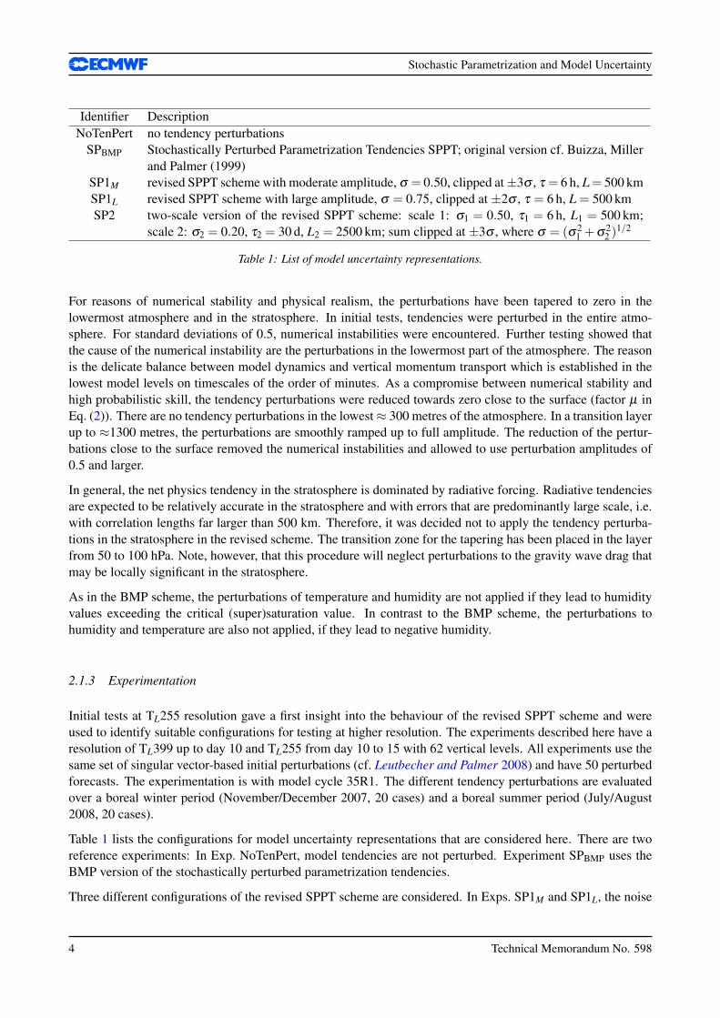
Figure 1: Example of the pattern r used in the revised scheme; contour interval 0.25; red (blue) contours correspond topositive(negative) values.
r has a horizontal correlation length scale of 500 km and a correlation time of 6 h. Thus the spatio-temporalcoherence of the noise is roughly similar to the original BMP version. Figure 1 shows a particular realisationof the pattern for SP1M in three-hourly intervals. The standard deviation of the random pattern r has been setto 0.50 and 0.75 in SP1M and SP1L, respectively. Coarse-graining diagnostic of Cloud Resolving Model outputby Shutts and Palmer (2007) suggests that an uncertainty of this magnitude is not unrealistic (cf. Section 5).
In Exp. SP2, the pattern r is the sum of two independent patterns r1 and r2 that represent errors on differentspatial and temporal scales. Both patterns r1 and r2 are defined by the same algorithm used for SP1M andSP1L. Pattern r1 represents fast evolving synoptic scale errors and has the same correlation characteristicsand amplitude as the pattern in SP1M. Pattern r2 represents slower evolving, planetary scale errors; it hasa correlation length scale of 2500 km and a correlation time of 30 d. The standard deviation of r2 is set to0.20. Therefore, the sum of r1 and r2 has a standard deviation of 0.54. Now, the different experiments will becompared in terms of upper air verification and precipitation.
2.1.4 Results: Upper air verification
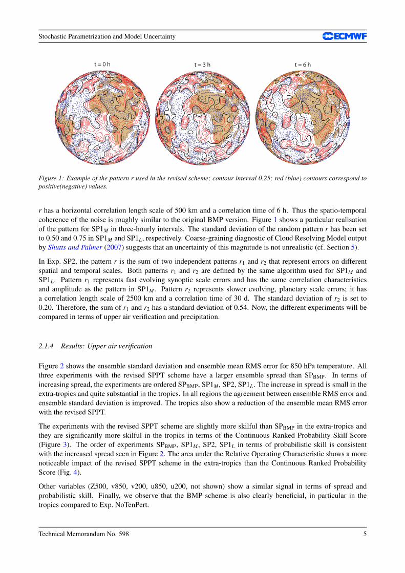
Figure 2 shows the ensemble standard deviation and ensemble mean RMS error for 850 hPa temperature. Allthree experiments with the revised SPPT scheme have a larger ensemble spread than SPBMP. In terms ofincreasing spread, the experiments are ordered SPBMP, SP1M, SP2, SP1L. The increase in spread is small in theextra-tropics and quite substantial in the tropics. In all regions the agreement between ensemble RMS error andensemble standard deviation is improved. The tropics also show a reduction of the ensemble mean RMS errorwith the revised SPPT.
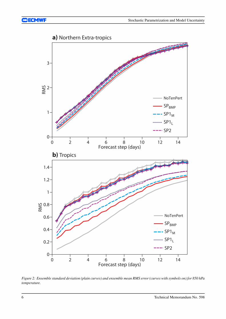
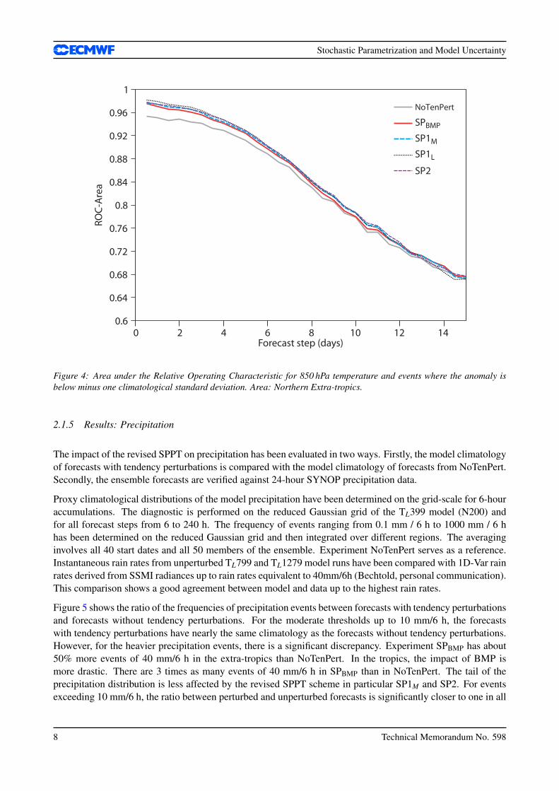
The experiments with the revised SPPT scheme are slightly more skilful than SPBMP in the extra-tropics andthey are significantly more skilful in the tropics in terms of the Continuous Ranked Probability Skill Score(Figure 3). The order of experiments SPBMP, SP1M, SP2, SP1L in terms of probabilistic skill is consistentwith the increased spread seen in Figure 2. The area under the Relative Operating Characteristic shows a morenoticeable impact of the revised SPPT scheme in the extra-tropics than the Continuous Ranked ProbabilityScore (Fig. 4).
Other variables (Z500, v850, v200, u850, u200, not shown) show a similar signal in terms of spread andprobabilistic skill. Finally, we observe that the BMP scheme is also clearly beneficial, in particular in thetropics compared to Exp. NoTenPert.
Technical Memorandum No. 598 5
Stochastic Parametrization and Model Uncertainty
Forecast step (days)
0
1
2
3
RMS
NoTenPert
SPBMP
SP1M
SP1L
SP2
NoTenPert
SPBMP
SP1M
SP1L
SP2
Forecast step (days)
0
0.2
0.4
0.6
0.8
1
1.2
1.4
RMS
0 2 4 6 8 10 12 14
0 2 4 6 8 10 12 14
a) Northern Extra-tropics
b) Tropics
Figure 2: Ensemble standard deviation (plain curves) and ensemble mean RMS error (curves with symbols on) for 850 hPatemperature.
6 Technical Memorandum No. 598
Stochastic Parametrization and Model Uncertainty
Forecast step (days)
NoTenPert
SPBMP
SP1M
SP1L
SP2
NoTenPert
SPBMP
SP1M
SP1L
SP2
Forecast step (days)
0 2 4 6 8 10 12 14
0 2 4 6 8 10 12 14
0
0.1
0.2
0.3
0.4
0.5
0.6
0.7
0.8
0.9CR
PSS
0.06
0
0.12
0.18
0.24
0.3
0.36
0.42
0.48
0.54
0.6
CRPS
Sa) Northern Extra-tropics
b) Tropics
Figure 3: Continuous Ranked Probability Skill Score for 850 hPa temperature.
Technical Memorandum No. 598 7
Stochastic Parametrization and Model Uncertainty
Forecast step (days)
0.6
0.64
0.68
0.72
0.76
0.8
0.84
0.88
0.92
0.96
1RO
C-A
rea
NoTenPert
SPBMP
SP1M
SP1L
SP2
0 2 4 6 8 10 12 14
Figure 4: Area under the Relative Operating Characteristic for 850 hPa temperature and events where the anomaly isbelow minus one climatological standard deviation. Area: Northern Extra-tropics.
2.1.5 Results: Precipitation
The impact of the revised SPPT on precipitation has been evaluated in two ways. Firstly, the model climatologyof forecasts with tendency perturbations is compared with the model climatology of forecasts from NoTenPert.Secondly, the ensemble forecasts are verified against 24-hour SYNOP precipitation data.
Proxy climatological distributions of the model precipitation have been determined on the grid-scale for 6-houraccumulations. The diagnostic is performed on the reduced Gaussian grid of the TL399 model (N200) andfor all forecast steps from 6 to 240 h. The frequency of events ranging from 0.1 mm / 6 h to 1000 mm / 6 hhas been determined on the reduced Gaussian grid and then integrated over different regions. The averaginginvolves all 40 start dates and all 50 members of the ensemble. Experiment NoTenPert serves as a reference.Instantaneous rain rates from unperturbed TL799 and TL1279 model runs have been compared with 1D-Var rainrates derived from SSMI radiances up to rain rates equivalent to 40mm/6h (Bechtold, personal communication).This comparison shows a good agreement between model and data up to the highest rain rates.
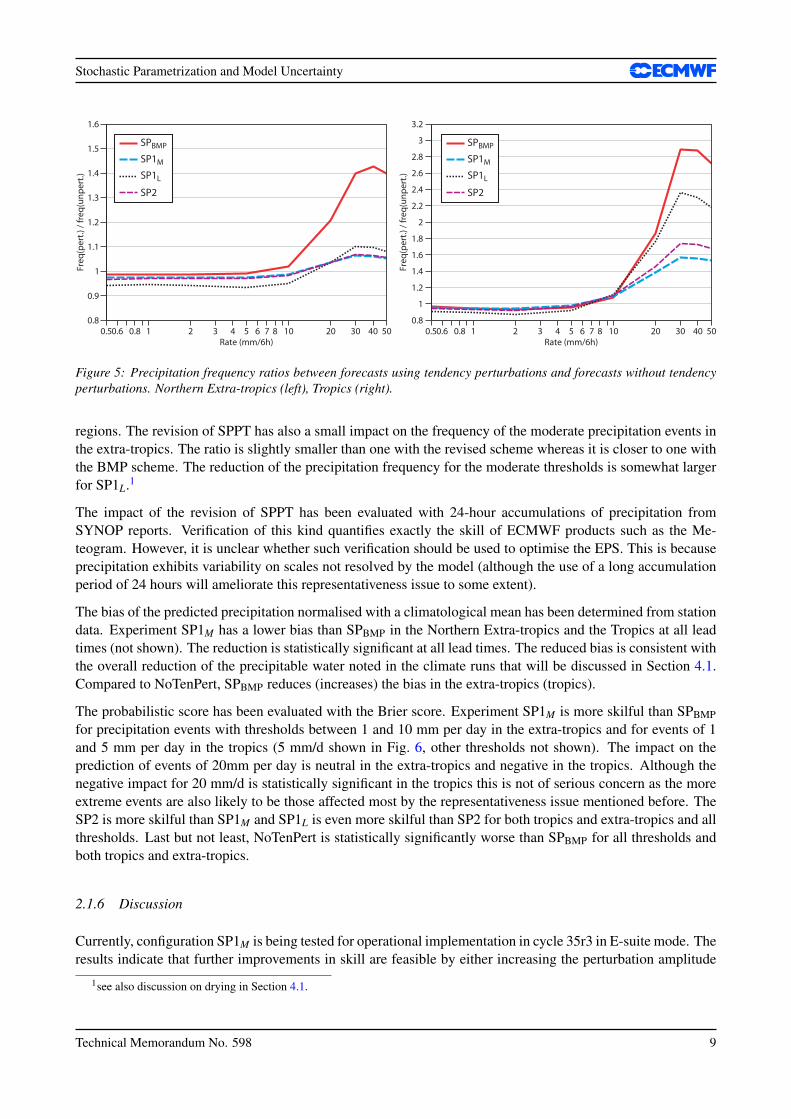
Figure 5 shows the ratio of the frequencies of precipitation events between forecasts with tendency perturbationsand forecasts without tendency perturbations. For the moderate thresholds up to 10 mm/6 h, the forecastswith tendency perturbations have nearly the same climatology as the forecasts without tendency perturbations.However, for the heavier precipitation events, there is a significant discrepancy. Experiment SPBMP has about50% more events of 40 mm/6 h in the extra-tropics than NoTenPert. In the tropics, the impact of BMP ismore drastic. There are 3 times as many events of 40 mm/6 h in SPBMP than in NoTenPert. The tail of theprecipitation distribution is less affected by the revised SPPT scheme in particular SP1M and SP2. For eventsexceeding 10 mm/6 h, the ratio between perturbed and unperturbed forecasts is significantly closer to one in all
8 Technical Memorandum No. 598
Stochastic Parametrization and Model Uncertainty
5040302010876543210.80.60.5Rate (mm/6h)
0.8
0.9
1
1.1
1.2
1.3
1.4
1.5
1.6
Freq
(per
t.) /
freq
(unp
ert.)
5040302010876543210.80.60.5Rate (mm/6h)
0.8
1
1.2
1.4
1.6
1.8
2
2.2
2.4
2.6
2.8
3
3.2
Freq
(per
t.) /
freq
(unp
ert.)
SPBMP
SP1M
SP1L
SP2
SPBMP
SP1M
SP1L
SP2
Figure 5: Precipitation frequency ratios between forecasts using tendency perturbations and forecasts without tendencyperturbations. Northern Extra-tropics (left), Tropics (right).
regions. The revision of SPPT has also a small impact on the frequency of the moderate precipitation events inthe extra-tropics. The ratio is slightly smaller than one with the revised scheme whereas it is closer to one withthe BMP scheme. The reduction of the precipitation frequency for the moderate thresholds is somewhat largerfor SP1L.1
The impact of the revision of SPPT has been evaluated with 24-hour accumulations of precipitation fromSYNOP reports. Verification of this kind quantifies exactly the skill of ECMWF products such as the Me-teogram. However, it is unclear whether such verification should be used to optimise the EPS. This is becauseprecipitation exhibits variability on scales not resolved by the model (although the use of a long accumulationperiod of 24 hours will ameliorate this representativeness issue to some extent).
The bias of the predicted precipitation normalised with a climatological mean has been determined from stationdata. Experiment SP1M has a lower bias than SPBMP in the Northern Extra-tropics and the Tropics at all leadtimes (not shown). The reduction is statistically significant at all lead times. The reduced bias is consistent withthe overall reduction of the precipitable water noted in the climate runs that will be discussed in Section 4.1.Compared to NoTenPert, SPBMP reduces (increases) the bias in the extra-tropics (tropics).
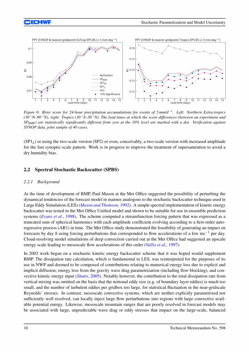
The probabilistic score has been evaluated with the Brier score. Experiment SP1M is more skilful than SPBMPfor precipitation events with thresholds between 1 and 10 mm per day in the extra-tropics and for events of 1and 5 mm per day in the tropics (5 mm/d shown in Fig. 6, other thresholds not shown). The impact on theprediction of events of 20mm per day is neutral in the extra-tropics and negative in the tropics. Although thenegative impact for 20 mm/d is statistically significant in the tropics this is not of serious concern as the moreextreme events are also likely to be those affected most by the representativeness issue mentioned before. TheSP2 is more skilful than SP1M and SP1L is even more skilful than SP2 for both tropics and extra-tropics and allthresholds. Last but not least, NoTenPert is statistically significantly worse than SPBMP for all thresholds andboth tropics and extra-tropics.
2.1.6 Discussion
Currently, configuration SP1M is being tested for operational implementation in cycle 35r3 in E-suite mode. Theresults indicate that further improvements in skill are feasible by either increasing the perturbation amplitude
1see also discussion on drying in Section 4.1.
Technical Memorandum No. 598 9
Stochastic Parametrization and Model Uncertainty
1 2 3 4 5 6 7 8 9 10 11 12 13 14 15Lead time (days)
0.08
0.1
0.07
0.09
BS
NoTenPertSPBMPSP1MSP1LSP210% Significance
PPT (SYNOP & nearest gridpoint) ExTrop EPS BS (≥ 5 mm day−1)
1 2 3 4 5 6 7 8 9 10 11 12 13 14 15Lead time (days)
0.12
0.13
0.14
0.15
0.16
BS
PPT (SYNOP & nearest gridpoint) Tropics EPS BS (≥ 5 mm day−1)
Figure 6: Brier score for 24-hour precipitation accumulations for events of 5 mm/d−1. Left: Northern Extra-tropics(30 N–90 N), right: Tropics (30 S–30 N). The lead times at which the score differences (between an experiment andSPBMP) are statistically significantly different from zero at the 10% level are marked with a dot. Verification againstSYNOP data, joint sample of 40 cases.
(SP1L) or using the two-scale version (SP2) or even, conceivably, a two-scale version with increased amplitudefor the fast synoptic-scale pattern. Work is in progress to improve the treatment of supersaturation to avoid adry humidity bias.
2.2 Spectral Stochastic Backscatter (SPBS)
2.2.1 Background
At the time of development of BMP, Paul Mason at the Met Office suggested the possibility of perturbing thedynamical tendencies of the forecast model in manner analogous to the stochastic backscatter technique used inLarge Eddy Simulation (LES) (Mason and Thomson, 1992). A simple spectral implementation of kinetic energybackscatter was tested in the Met Office Unified model and shown to be suitable for use in ensemble predictionsystems (Evans et al., 1998). The scheme computed a streamfunction forcing pattern that was expressed as atruncated sum of spherical harmonics with each amplitude coefficient evolving according to a first-order auto-regressive process (AR1) in time. The Met Office study demonstrated the feasibility of generating an impact onforecasts by day 8 using forcing perturbations that corresponded to flow accelerations of a few ms−1 per day.Cloud-resolving model simulations of deep convection carried out at the Met Office had suggested an upscaleenergy scale leading to mesoscale flow accelerations of this order (Vallis et al., 1997).
In 2003 work began on a stochastic kinetic energy backscatter scheme that it was hoped would supplementBMP. The dissipation rate calculation, which is fundamental to LES, was reinterpreted for the purposes of itsuse in NWP and deemed to be composed of contributions relating to numerical energy loss due to explicit andimplicit diffusion; energy loss from the gravity wave drag parametrization (including flow blocking), and con-vective kinetic energy input (Shutts, 2005). Notably however, the contribution to the total dissipation rate fromvertical mixing was omitted on the basis that the notional eddy size (e.g. of boundary layer eddies) is much toosmall, and the number of turbulent eddies per gridbox too large, for statistical fluctuation in the near-gridscaleReynolds’ stresses. In contrast, mesoscale convective systems, which are neither explicitly parametrized norsufficiently well resolved, can locally inject large flow perturbations into regions with large convective avail-able potential energy. Likewise, mesoscale mountain ranges that are poorly resolved in forecast models maybe associated with large, unpredictable wave drag or eddy stresses that impact on the large-scale, balanced
10 Technical Memorandum No. 598
Stochastic Parametrization and Model Uncertainty
dynamics.
By perturbing streamfunction (or equivalently vorticity), the forecast model responds with less noise than if thewind components were independently perturbed (in fact options exist in the present code to compute temper-ature perturbations consistent with the linear or non-linear balance equations). Unlike stochastic backscatter’suse in LES, the streamfunction forcing perturbations in the IFS are horizontally non-divergent and provide sub-stantial energy input across the whole spectrum of wavenumbers. As will be seen later, generating sufficientimpact on ensemble spread requires considerable input of energy in the sub-synoptic scales of motion. In thisrespect our approach to backscatter differs from Frederiksen and Davies (1997) who consider upscale energytransfer in two-dimensional flow on the sphere. Their work emphasises the injection of energy near the trunca-tion scale of a forecast model whereas stochastic backscatter includes upscale energy transfer from unbalancedmotions associated with convection and gravity waves.
The first stochastic backscatter scheme tested at ECMWF was called CASBS (Cellular Automaton StochasticBackscatter) and used a Cellular Automaton (CA) pattern generator to define the form of the streamfunctionforcing field. As in LES backscatter, the amplitude of the forcing function was modulated by the square-rootof a dissipation rate field. The choice of a CA was originally motivated by the idea of generating patterns thatwould resemble the organization of convective cloud clusters in which the scale and evolution of the patternscould be linked to the local large-scale flow through their corresponding rulesets (Palmer, 2001). Whilst thisapproach is still under investigation using probabilistic CAs, a more pragmatic approach was to revert to theoriginal spectrally-based scheme that had been tested at the Met Office.
Using a triangularly-truncated spherical harmonic expansion it is possible to ensure that the streamfunctionforcing field is spatially-isotropic on the sphere and has a power spectrum of a chosen form. The auto-correlation time scale of the AR1 process for the spectral coefficients can also be made a function of wavenum-ber and calibrated using the procedure outlined in Section 5. The resulting scheme, called Spectral StochasticBackscatter Scheme (SPBS) is described fully in Berner et al. (2009b) and has been the subject of consider-able development in the last year. A major new extension not present in the Berner et al formulation is theintroduction of vertical phase correlations for which autocorrelation scale is a function of horizontal spectralwavenumber.
2.2.2 The pattern generator and net streamfunction forcing
SPBS is conveniently formulated in terms of a streamfunction forcing function (Fψ ) prescribed on each modellevel and given by:
Fψ =(
bRDtot
Btot
)1/2
Fψ∗ (3)
where Fψ∗ is a three-dimensional random pattern field constructed to have specific statistical properties andwhich, if used by itself as a streamfunction forcing, would imply an ensemble-mean energy input rate of Btot .Dtot(x,y,z, t) is the total dissipation rate and bR is a backscatter ratio so that the factor (bRDtot/Btot)
1/2 locallyrescales the energy input rate to be bRDtot . Since Fψ only affects the rotational wind, it is less likely to destroythe dynamical balance between pressure and wind fields than an arbitrary wind forcing. The spectral powerdistribution pattern field is assumed to be of the form of a power law in spherical harmonic degree n with theexponent inferred from a coarse-graining procedure (see Section 5). In all of the forecasts presented here thatuse SPBS, the auto-correlation time scale is set 25000 s (i.e. ≈ 7 hours). Further mathematical details of SPBScan be found in Appendix 8.2.
Technical Memorandum No. 598 11
Stochastic Parametrization and Model Uncertainty
2.2.3 The dissipation rate calculation
The total dissipation rate Dtot is computed on all model levels and is made up of three components:
• numerical dissipation rate (Dnum) as an estimate of the combined contributions from explicit biharmonicdiffusion and interpolation error in the semi-Lagrangian advection scheme
• the combined effect of kinetic energy dissipation due to orographic Gravity Wave Drag (GWD) and flowblocking (DGWD)
• the rate of kinetic energy export from sub-gridscale deep convection into the resolved flow (Dcon).
The numerical kinetic energy dissipation rate is given by the expression
Dnum = αnumK |∇ζ |2 (4)
where ζ is the relative vorticity, K is the bi-harmonic diffusion coefficient and αnum is a factor to augment thedissipation rate to include the effects of semi-Lagrangian interpolation error (currently set to 3).
The gravity wave/mountain drag contribution to the energy dissipation rate (DGWD) is obtained simply as thevector product of the parametrized wind vector tendency with the wind itself.
The convective contribution is not a dissipation rate as such but a term that represents the rate of transformationof convectively-generated kinetic energy to quasi-balanced, resolved flow. Specifically, Dcon is given by:
Dcon = αcon
(sin(φ)+
ζ
2Ω
)2
Mdρw2 (5)
where αcon is an area fraction factor, φ is latitude, Ω is the Earth’s rotation rate, Md is the convective massdetrainment rate and w is a vertically-averaged convective updraught velocity. Excluding the bracketed factor,this term is a parametrization for the rate of detrainment of convective cloud kinetic energy to the resolvedscales. The bracketed factor is a normalized absolute vorticity equivalent to (ζ + f )/2Ω. It approximatelyexpresses the fraction of the kinetic energy released that is captured in balanced motion and will be referredto as the ‘inertial stability factor’ (Shutts and Gray, 1994). Deep convective mass transfer creates distinctivepotential vorticity (PV) features in an environment with background PV. Near the equator, the background PV isvery weak and so most of the convective energy release goes into unbalanced modes whereas in middle latitudesmesoscale convective systems generate intense PV anomalies that influence the development of baroclinic wavesystems.
The streamfunction forcing Fψ given by eq. (3) is evolved in time for each EPS member using the AR1 processdefined in eq. (21) (see appendix) and the different random number sets r j
m,n ensure different model error forcingpatterns.
2.2.4 Impacts in the IFS
Our results focus on ensemble forecasts with start dates in July and August so that the effect on tropical cyclonefrequency could be monitored. Early experience had shown that SPBS in conjunction with SPBMP led to anexcessively high frequency of tropical cyclones and tropical depressions. In this section, attention will befocused on the temperature at 850 hPa (T850) and for reference the corresponding results for SP1M are shown.
12 Technical Memorandum No. 598
Stochastic Parametrization and Model Uncertainty
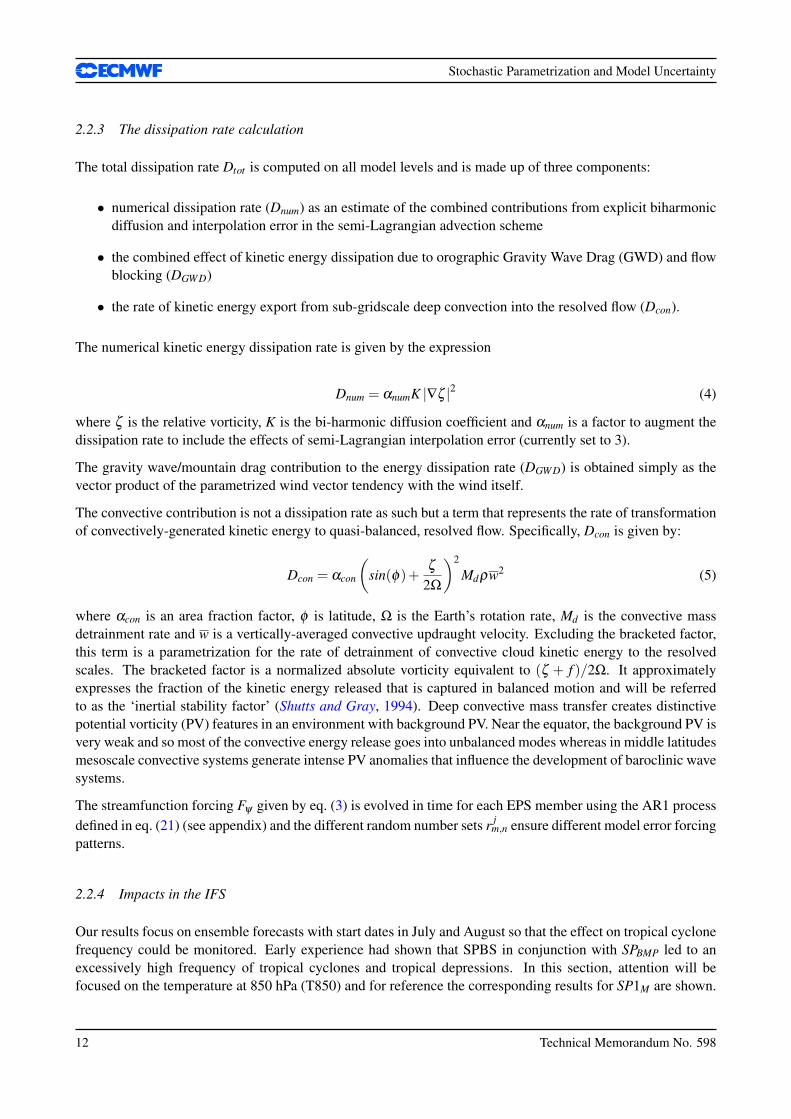
Figure 7 shows the error of the ensemble-mean and spread (left column) together with the associated Con-tinuous Rank Probability Skill Score (CRPSS; right column) for TL255 ensemble forecasts made with (i) nostochastic tendency perturbations; (ii) revised SPPT (SP1M) and (iii) SPBS alone with bR = 0.085. It can beseen that the impact of SPBS is comparable with SP1M except in the first 3 days where SPBS produces less addi-tional spread compared to SP1M. This is probably due to the fact that SPBS does not directly force temperaturewhereas SPPT does. Both SPBS and SP1M substantially increase ensemble spread (particularly in the tropics)and this is reflected in the CRPSS which are increased over the forecasts without stochastic perturbations. Theerror in the ensemble-mean is reduced with the biggest reduction being in the tropics with SPBS.
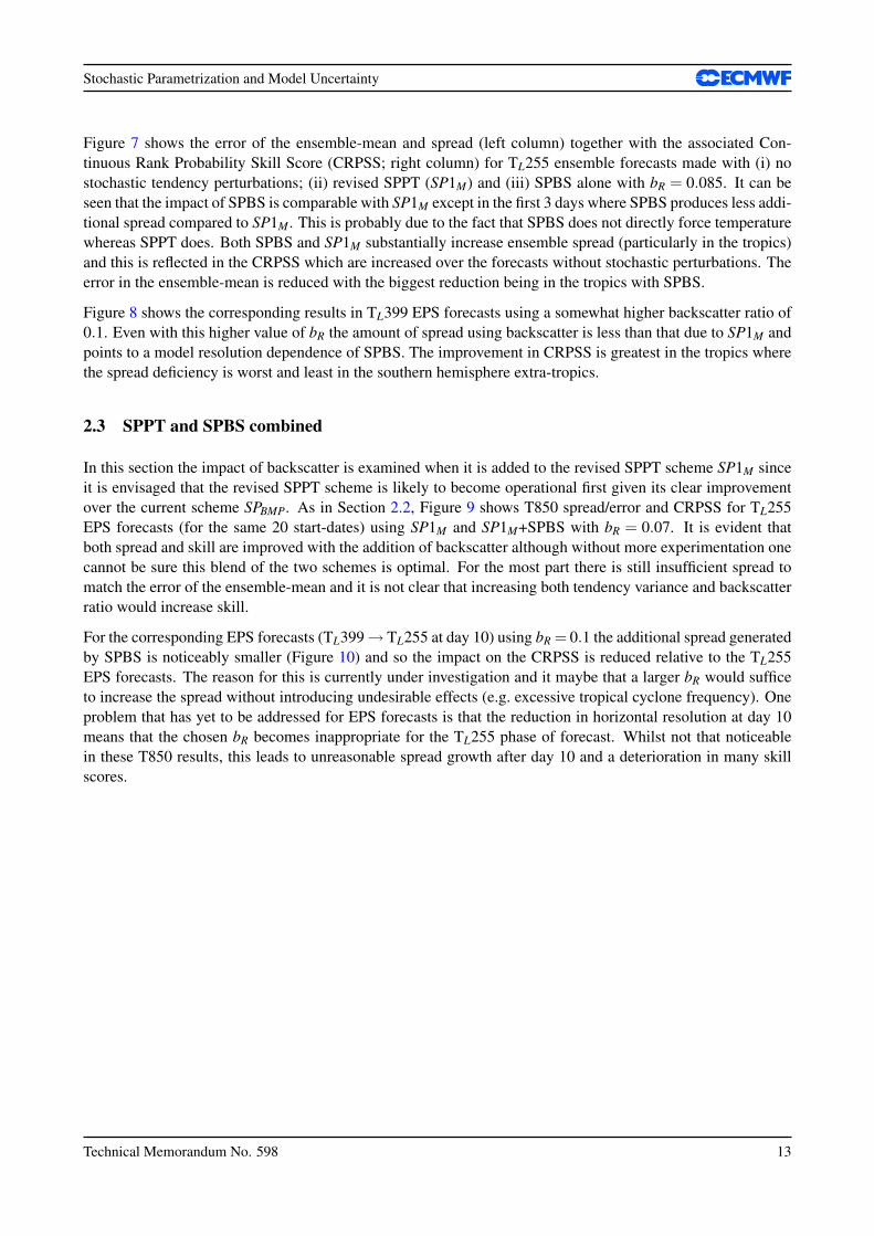
Figure 8 shows the corresponding results in TL399 EPS forecasts using a somewhat higher backscatter ratio of0.1. Even with this higher value of bR the amount of spread using backscatter is less than that due to SP1M andpoints to a model resolution dependence of SPBS. The improvement in CRPSS is greatest in the tropics wherethe spread deficiency is worst and least in the southern hemisphere extra-tropics.
2.3 SPPT and SPBS combined
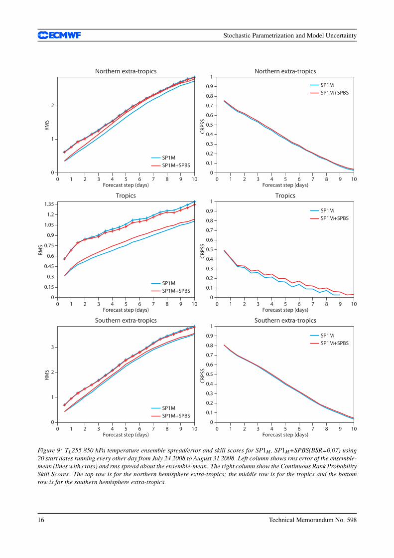
In this section the impact of backscatter is examined when it is added to the revised SPPT scheme SP1M sinceit is envisaged that the revised SPPT scheme is likely to become operational first given its clear improvementover the current scheme SPBMP. As in Section 2.2, Figure 9 shows T850 spread/error and CRPSS for TL255EPS forecasts (for the same 20 start-dates) using SP1M and SP1M+SPBS with bR = 0.07. It is evident thatboth spread and skill are improved with the addition of backscatter although without more experimentation onecannot be sure this blend of the two schemes is optimal. For the most part there is still insufficient spread tomatch the error of the ensemble-mean and it is not clear that increasing both tendency variance and backscatterratio would increase skill.
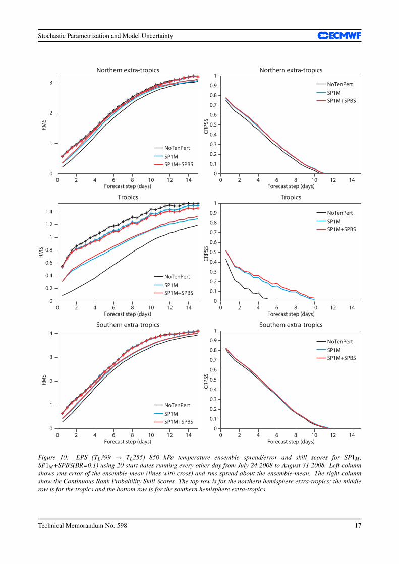
For the corresponding EPS forecasts (TL399→ TL255 at day 10) using bR = 0.1 the additional spread generatedby SPBS is noticeably smaller (Figure 10) and so the impact on the CRPSS is reduced relative to the TL255EPS forecasts. The reason for this is currently under investigation and it maybe that a larger bR would sufficeto increase the spread without introducing undesirable effects (e.g. excessive tropical cyclone frequency). Oneproblem that has yet to be addressed for EPS forecasts is that the reduction in horizontal resolution at day 10means that the chosen bR becomes inappropriate for the TL255 phase of forecast. Whilst not that noticeablein these T850 results, this leads to unreasonable spread growth after day 10 and a deterioration in many skillscores.
Technical Memorandum No. 598 13
Stochastic Parametrization and Model Uncertainty
Forecast step (days)
0
1
2
RMS
Northern extra-tropics
0
0.1
0.2
0.3
0.4
0.5
0.6
0.7
0.8
0.9
1
CRPS
S
Northern extra-tropics
0
0.15
0.3
0.45
0.6
0.75
0.9
1.05
1.2
1.35
RMS
Tropics
0
0.1
0.2
0.3
0.4
0.5
0.6
0.7
0.8
0.9
1CR
PSS
Tropics
0
1
2
3
RMS
Southern extra-tropics
NoTenPert
SP1MSPBS
NoTenPert
SP1MSPBS
NoTenPert
SP1MSPBS
NoTenPert
SP1MSPBS
NoTenPert
SP1MSPBS
NoTenPert
SP1MSPBS
0
0.1
0.2
0.3
0.4
0.5
0.6
0.7
0.8
0.9
1
CRPS
S
Southern extra-tropics
0 1 2 3 4 5 6 7 8 9 10Forecast step (days)
0 1 2 3 4 5 6 7 8 9 10
Forecast step (days)0 1 2 3 4 5 6 7 8 9 10
Forecast step (days)0 1 2 3 4 5 6 7 8 9 10
Forecast step (days)0 1 2 3 4 5 6 7 8 9 10
Forecast step (days)0 1 2 3 4 5 6 7 8 9 10
Figure 7: TL255 850 hPa temperature ensemble spread/error and skill scores for NoTendPert, SP1M and SPBS(BSR=0.085) using 20 start dates running every other day from July 24 2008 to August 31 2008. Left column showsrms error of the ensemble-mean (lines with cross) and rms spread about the ensemble-mean. The right column show theContinuous Rank Probability Skill Scores. The top row is for the northern hemisphere extra-tropics; the middle row is forthe tropics and the bottom row is for the southern hemisphere extra-tropics.
14 Technical Memorandum No. 598
Stochastic Parametrization and Model Uncertainty
Forecast step (days)
Northern extra-tropics
0
0.1
0.2
0.3
0.4
0.5
0.6
0.7
0.8
0.9
1
CRPS
S
Northern extra-tropics
Tropics
0
0.1
0.2
0.3
0.4
0.5
0.6
0.7
0.8
0.9
1CR
PSS
Tropics
Southern extra-tropics
NoTenPert
SP1MSPBS
NoTenPert
SP1MSPBS
NoTenPert
SP1MSPBS
NoTenPert
SP1MSPBS
NoTenPert
SP1MSPBS
NoTenPert
SP1MSPBS
0
0.1
0.2
0.3
0.4
0.5
0.6
0.7
0.8
0.9
1
CRPS
S
Southern extra-tropics
0
1
2
3
RMS
0
0.2
0.4
0.6
0.8
1
1.2
1.4
RMS
0
1
2
3
4
RMS
0 2 4 6 8 10 12 14
Forecast step (days)0 2 4 6 8 10 12 14
Forecast step (days)0 2 4 6 8 10 12 14
Forecast step (days)0 2 4 6 8 10 12 14
Forecast step (days)0 2 4 6 8 10 12 14
Forecast step (days)0 2 4 6 8 10 12 14
Figure 8: EPS (TL399 → TL255) 850 hPa temperature ensemble spread/error and skill scores for NoTendPert, SP1Mand SPBS(BSR=0.1) 20 start dates running every other day from July 24 2008 to August 31 2008. Left column showsrms error of the ensemble-mean (lines with cross) and rms spread about the ensemble-mean. The right column show theContinuous Rank Probability Skill Scores. The top row is for the northern hemisphere extra-tropics; the middle row is forthe tropics and the bottom row is for the southern hemisphere extra-tropics.
Technical Memorandum No. 598 15
Stochastic Parametrization and Model Uncertainty
0
1
2
RMS
Northern extra-tropics
0
0.1
0.2
0.3
0.4
0.5
0.6
0.7
0.8
0.9
1
CRPS
S
Northern extra-tropics
0
0.15
0.3
0.45
0.6
0.75
0.9
1.05
1.2
1.35
RMS
Tropics
0
0.1
0.2
0.3
0.4
0.5
0.6
0.7
0.8
0.9
1CR
PSS
Tropics
0
1
2
3
RMS
Southern extra-tropics
0
0.1
0.2
0.3
0.4
0.5
0.6
0.7
0.8
0.9
1
CRPS
S
Southern extra-tropics
Forecast step (days)1 2 3 4 5 6 7 8 9 10
Forecast step (days)1 2 3 4 5 6 7 8 9 10
Forecast step (days)0 1 2 3 4 5 6 7 8 9 10
SP1MSP1M+SPBS
SP1MSP1M+SPBS
SP1MSP1M+SPBS
SP1MSP1M+SPBS
SP1MSP1M+SPBS
SP1MSP1M+SPBS
Forecast step (days)1 2 3 4 5 6 7 8 9 10
Forecast step (days)1 2 3 4 5 6 7 8 9 10
Forecast step (days)0
0 0
0 0
1 2 3 4 5 6 7 8 9 10
Figure 9: TL255 850 hPa temperature ensemble spread/error and skill scores for SP1M , SP1M+SPBS(BSR=0.07) using20 start dates running every other day from July 24 2008 to August 31 2008. Left column shows rms error of the ensemble-mean (lines with cross) and rms spread about the ensemble-mean. The right column show the Continuous Rank ProbabilitySkill Scores. The top row is for the northern hemisphere extra-tropics; the middle row is for the tropics and the bottomrow is for the southern hemisphere extra-tropics.
16 Technical Memorandum No. 598
Stochastic Parametrization and Model Uncertainty
Forecast step (days)
Northern extra-tropics
0
0.1
0.2
0.3
0.4
0.5
0.6
0.7
0.8
0.9
1
CRPS
S
Northern extra-tropics
Tropics
0
0.1
0.2
0.3
0.4
0.5
0.6
0.7
0.8
0.9
1CR
PSS
Tropics
Southern extra-tropics
0
0.1
0.2
0.3
0.4
0.5
0.6
0.7
0.8
0.9
1
CRPS
S
Southern extra-tropics
0
1
2
3
RMS
0
0.2
0.4
0.6
0.8
1
1.2
1.4
RMS
0
1
2
3
4
RMS
0 2 4 6 8 10 12 14
Forecast step (days)0 2 4 6 8 10 12 14
Forecast step (days)0 2 4 6 8 10 12 14
Forecast step (days)0 2 4 6 8 10 12 14
Forecast step (days)0 2 4 6 8 10 12 14
Forecast step (days)0 2 4 6 8 10 12 14
NoTenPert
SP1MSP1M+SPBS
NoTenPert
SP1MSP1M+SPBS
NoTenPert
SP1MSP1M+SPBS
NoTenPert
SP1MSP1M+SPBS
NoTenPert
SP1MSP1M+SPBS
NoTenPert
SP1MSP1M+SPBS
Figure 10: EPS (TL399 → TL255) 850 hPa temperature ensemble spread/error and skill scores for SP1M ,SP1M+SPBS(BR=0.1) using 20 start dates running every other day from July 24 2008 to August 31 2008. Left columnshows rms error of the ensemble-mean (lines with cross) and rms spread about the ensemble-mean. The right columnshow the Continuous Rank Probability Skill Scores. The top row is for the northern hemisphere extra-tropics; the middlerow is for the tropics and the bottom row is for the southern hemisphere extra-tropics.
Technical Memorandum No. 598 17
Stochastic Parametrization and Model Uncertainty
3 Use of stochastic parametrization schemes in ensemble data assimilation
One of the key aspects that ensemble prediction systems need to simulate to provide accurate probabilisticpredictions is the effect on forecast error of initial uncertainties. At ECMWF these uncertainties have beensimulated with singular vectors (SVs), perturbations characterized by the fastest growth, measured using a totalenergy norm (Buizza and Palmer, 1995; Palmer et al., 1998), over a finite time interval. In the current systemdifferent sets of singular vectors are used to better sample the initial uncertainties. Initial-time SVs growinginto the first 48 hours of the forecast range, which represent uncertainties growing during the forecast time, aremixed with evolved SVs computed to grow during the 48 hours leading to the analysis time, which representuncertainties that have been growing during the current and past data-assimilation cycles. The initial-time andevolved SVs are combined and scaled to have an amplitude comparable to the analysis error estimate providedby the ECMWF data assimilation system (Barkmeijer et al., 1999).
Buizza et al. (2008) showed that perturbations defined by an ensemble data assimilation (EDA) system pro-vide a better representation of the uncertainties growing during the data assimilation cycle than the set of theevolved singular vectors currently used in the operational EPS. In their work, ensembles of 10 perturbed and1 unperturbed analyses were generated by randomly perturbing the observations in each single assimilationcycle at TL399L91 resolution, with a 12-hour 4D-Var with TL159L91 inner loops, and by including a versionof the stochastic backscatter scheme (Shutts, 2005; Berner et al., 2009b). For each observation (apart fromcloud-track winds) perturbations were defined by randomly sampling a Gaussian distribution with zero meanand standard deviation defined by the observation error standard deviation. For cloud-track wind observations,perturbations were horizontally correlated (Bormann et al., 2003). Sea-surface temperature fields were alsoperturbed with correlated patterns as in the current operational ECMWF seasonal ensemble forecasting system(Vialard et al., 2005). Buizza et al. (2008)’s results indicated that if used alone to define EPS initial uncer-tainties, EDA-based perturbations lead to an under-dispersive and less skilful ensemble then the one based oninitial-time SVs only. By contrast, combining the EDA and the initial-time SVs improves the ensemble spread,reduces the ensemble-mean error, and provides more skilful probabilistic forecasts than the current operationalsystem based on initial-time and evolved SVs.
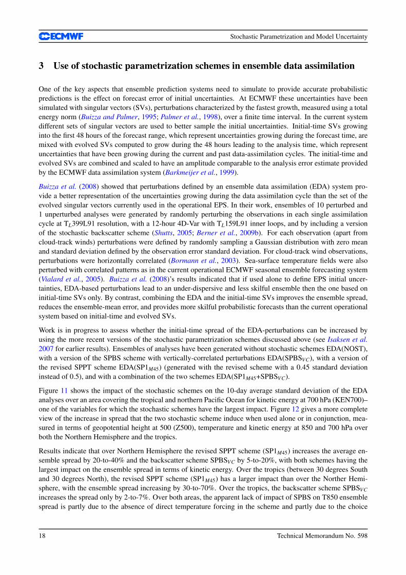
Work is in progress to assess whether the initial-time spread of the EDA-perturbations can be increased byusing the more recent versions of the stochastic parametrization schemes discussed above (see Isaksen et al.2007 for earlier results). Ensembles of analyses have been generated without stochastic schemes EDA(NOST),with a version of the SPBS scheme with vertically-correlated perturbations EDA(SPBSVC), with a version ofthe revised SPPT scheme EDA(SP1M45) (generated with the revised scheme with a 0.45 standard deviationinstead of 0.5), and with a combination of the two schemes EDA(SP1M45+SPBSVC).
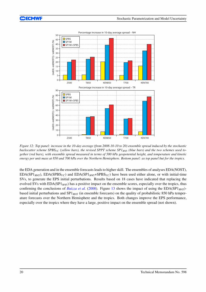
Figure 11 shows the impact of the stochastic schemes on the 10-day average standard deviation of the EDAanalyses over an area covering the tropical and northern Pacific Ocean for kinetic energy at 700 hPa (KEN700)–one of the variables for which the stochastic schemes have the largest impact. Figure 12 gives a more completeview of the increase in spread that the two stochastic scheme induce when used alone or in conjunction, mea-sured in terms of geopotential height at 500 (Z500), temperature and kinetic energy at 850 and 700 hPa overboth the Northern Hemisphere and the tropics.
Results indicate that over Northern Hemisphere the revised SPPT scheme (SP1M45) increases the average en-semble spread by 20-to-40% and the backscatter scheme SPBSVC by 5-to-20%, with both schemes having thelargest impact on the ensemble spread in terms of kinetic energy. Over the tropics (between 30 degrees Southand 30 degrees North), the revised SPPT scheme (SP1M45) has a larger impact than over the Norther Hemi-sphere, with the ensemble spread increasing by 30-to-70%. Over the tropics, the backscatter scheme SPBSVC
increases the spread only by 2-to-7%. Over both areas, the apparent lack of impact of SPBS on T850 ensemblespread is partly due to the absence of direct temperature forcing in the scheme and partly due to the choice
18 Technical Memorandum No. 598
Stochastic Parametrization and Model Uncertainty
20°S
0°
20°N
40°N
60°N
160°E 160°W 120°W
20°S
0°
20°N
40°N
60°N
160°E 160°W 120°W
20°S
0°
20°N
40°N
60°N
160°E 160°W 120°W
20°S
0°
20°N
40°N
60°N
160°E 160°W 120°W
0.5 1 1.5 2 2.5 3 3.5 4 4.5 5
Figure 11: Top-left panel: 10-day average (from 2008-10-10 to 20) std of the EDA measured in terms of kinetic energy perunit mass at 700 hPa generated without stochastic schemes. Top-right: difference between the std of the EDA generatedwith the revised SPPT scheme SP1M45 and without stochastic schemes. Bottom-left: difference between the std of theEDA generated with the stochastic backscatter scheme SPBSVC and without stochastic schemes. Bottom-right: differencebetween the std of the EDA generated with SP1M45+SPBSVC and without stochastic schemes. Contour interval: 0.5 m2/s2
for full field, and 0.25 m2/s2 for differences.
of backscatter ratio. For TL399 forecasts, a backscatter ratio of twice the value used here would have been amore appropriate choice. The experiments will be rerun using the latest implementations of the schemes, whichinclude a standard deviation of 0.5 for SPPT and a backscatter ratio of 0.1 for SPBS. Overall, the revised SPPTscheme (SP1M45) has a larger impact, and the combined use of the two schemes leads to a stronger impact onthe ensemble spread.
In data-assimilation, an ensemble of analyses can be used to compute flow-dependent background error statis-tics to improve the assimilation of observations (more specifically, the plan is to run the latest high-resolutiondata-assimilation cycle with background error statistics computed using a lower-resolution ensemble of analy-ses run during the previous data assimilation cycle). Work is in progress to assess the impact of the stochasticschemes on the spread of the EDA analyses, and thus on the background statistics.
In ensemble prediction, a very recent set of experiments has indicated that the use of the revised SPPT scheme in
Technical Memorandum No. 598 19
Stochastic Parametrization and Model Uncertainty
Percentage increase in 10-day average spread – NH
0
5
10
15
20
25
30
35
40
45
50
Z500 T850 KEN850 T700 KEN700
[std
(X)–
std(
NO
ST)]
/ std
(NO
ST) (
%)
Percentage increase in 10-day average spread – TR
0
10
20
30
40
50
60
70
80
90
Z500 T850 KEN850 T700 KEN700
[std
(X)–
std(
NO
ST)]
/ std
(NO
ST) (
%)
SPBSSP1MSP1M+SPBS
SPBSSP1MSP1M+SPBS
Figure 12: Top panel: increase in the 10-day average (from 2008-10-10 to 20) ensemble spread induced by the stochasticbackscatter scheme SPBSVC (yellow bars), the revised SPPT scheme SP1M45 (blue bars) and the two schemes used to-gether (red bars), with ensemble spread measured in terms of 500 hPa geopotential height, and temperature and kineticenergy per unit mass at 850 and 700 hPa over the Northern Hemisphere. Bottom panel: as top panel but for the tropics.
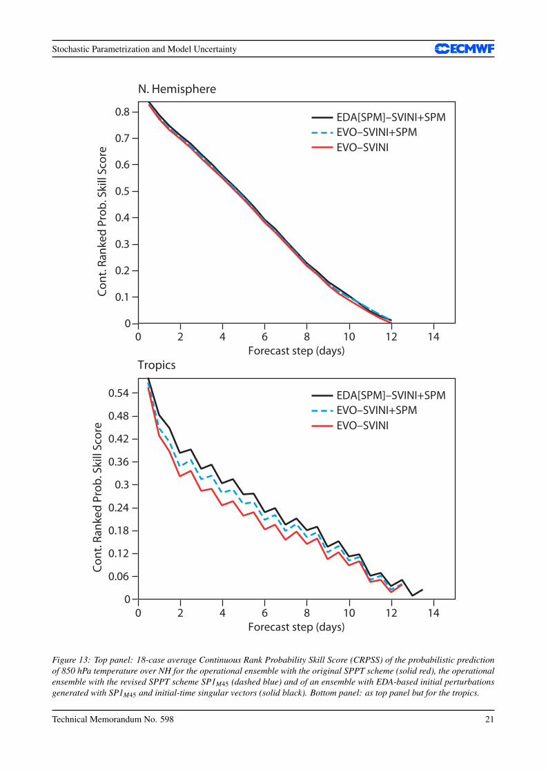
the EDA generation and in the ensemble forecasts leads to higher skill. The ensembles of analyses EDA(NOST),EDA(SP1M45), EDA(SPBSVC) and EDA(SP1M45+SPBSVC) have been used either alone, or with initial-timeSVs, to generate the EPS initial perturbations. Results based on 18 cases have indicated that replacing theevolved SVs with EDA(SP1M45) has a positive impact on the ensemble scores, especially over the tropics, thusconfirming the conclusions of Buizza et al. (2008). Figure 13 shows the impact of using the EDA(SP1M45)-based initial perturbations and SP1M45 (in ensemble forecasts) on the quality of probabilistic 850 hPa temper-ature forecasts over the Northern Hemisphere and the tropics. Both changes improve the EPS performance,especially over the tropics where they have a large, positive impact on the ensemble spread (not shown).
20 Technical Memorandum No. 598
Stochastic Parametrization and Model Uncertainty
Forecast step (days)
0
0.1
0.2
0.3
0.4
0.5
0.6
0.7
0.8Co
nt. R
anke
d Pr
ob. S
kill
Scor
eN. Hemisphere
EDA[SPM]–SVINI+SPMEVO–SVINI+SPMEVO–SVINI
EDA[SPM]–SVINI+SPMEVO–SVINI+SPMEVO–SVINI
0
0.06
0.12
0.18
0.24
0.3
0.36
0.42
0.48
0.54
Cont
. Ran
ked
Prob
. Ski
ll Sc
ore
Tropics
0 2 4 6 8 10 12 14
Forecast step (days)0 2 4 6 8 10 12 14
Figure 13: Top panel: 18-case average Continuous Rank Probability Skill Score (CRPSS) of the probabilistic predictionof 850 hPa temperature over NH for the operational ensemble with the original SPPT scheme (solid red), the operationalensemble with the revised SPPT scheme SP1M45 (dashed blue) and of an ensemble with EDA-based initial perturbationsgenerated with SP1M45 and initial-time singular vectors (solid black). Bottom panel: as top panel but for the tropics.
Technical Memorandum No. 598 21
Stochastic Parametrization and Model Uncertainty
4 Impact on seasonal integrations
As part of the routine assessment of changes in the physics of the IFS, long uncoupled (atmosphere-only)climate integrations are usually carried out at a relatively low horizontal resolution. Diagnosis of these longintegrations provides a good idea as to whether the proposed changes have neutral, positive or detrimental im-pacts on certain aspects of the model’s climate (Rodwell and Jung, 2008). Given that the implementation ofstochastic parametrization schemes constitutes a substantial modification of the physics of the IFS, it has beendecided to carry out a detailed investigation to understand the impact that the various stochastic parametrizationschemes have on the model’s climate. In fact, in previous studies it has been found that stochastic parametriza-tion generally improve the climate of the model, especially in terms of the extratropical atmospheric circulation(Jung et al., 2005; Palmer et al., 2005; Berner et al., 2009a). Results from these latest experiments are discussedin Section 4.1.
Since the operational introduction of System 3 in 2007, seasonal forecast and hindcast ensembles with thecoupled IFS-HOPE system have been using the original version of SPPT (SPBMP) for representing model un-certainty. However, the ensembles of seasonal integrations are, in general, underdispersive, i.e., the ensemblestandard deviation around the ensemble mean is substantially smaller than the RMSE of the ensemble mean.The lack of spread becomes apparent from the first month of the integrations and remains relatively constantover all lead times.
An earlier version of the stochastic backscatter scheme based on a cellular automaton pattern generator (CASBS)had been applied to a test set of seasonal hindcasts using the IFS atmospheric cycle CY29R2. The resultsshowed a reduction in some of the systematic errors, for example for tropical rainfall and SSTs in the ENSOregion, and significant improvements in probabilistic skill scores for a number of variables (Berner et al., 2008).
In the ENSEMBLES project, the CASBS simulations were compared with two alternative ways to addressmodel uncertainty on the seasonal time range, namely with a multi-model ensemble and a perturbed physicalparameter ensemble. It was found in Doblas-Reyes et al. (2009) that the multi-model ensemble performed beston lead times shorter than five months.
In Section 4.2 we discuss recent progress that has been made in coupled IFS-HOPE seasonal integrations withthe atmospheric cycle CY35R2 using the revised SPPT and SPBS schemes. A total of 3 different experimentswere performed: SP2 using the two-scale version of the revised SPPT scheme with the parameter settingsaccording to Table 1; SPBS with a backscatter ratio bR = 0.05; and the combination of SP2 + SPBS. Thecontrol experiment Ctrl was done using the original version of SPPT, SPBMP.
4.1 Systematic error in uncoupled integrations
In order to study the impact of the different stochastic parametrization schemes on the climate of the ECMWFmodel, a large set of 13-months long integrations, started on 15 November of each of the years 1990–2005,was carried out for the different model formulations summarized in Tab. 1. All integrations are based on cycle35R1 with a horizontal resolution of TL159 and 91 levels in the vertical. Observed SST and sea ice fields wereprescribed as lower boundary conditions. Here we analyse the impact of stochastic parametrization schemes onthe first season of the integrations only (i.e. DJF).
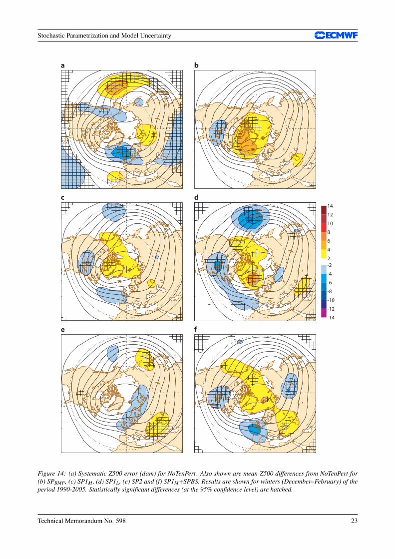
The impact on the wintertime atmospheric circulation over the Northern Hemisphere can be inferred fromFig. 14. Albeit much reduced compared to IFS cycles used before 2008 (Jung et al., 2009), there are stillnotable systematic Z500 error for NoTenPert (cycle 35R1) over the Northern Hemisphere, especially in thenortheastern North Atlantic and the North Pacific (Fig. 14a). Generally, mean Z500 differences between the
22 Technical Memorandum No. 598
Stochastic Parametrization and Model Uncertainty
-2
-2
-2
-2
-2
-2
-2
-2
2
2
2
2
2
a
-2
2
2
2
b
-2
-2
-2 2
2
e
-2
-2
-2
-2
-2
-2
-2
-2
2
2
2
2
d
-14
-12
-10
-8
-6
-4
-22
4
6
8
10
12
14
-2 -2
-2
-2
2
2
2
2
c
-2
-2
-2
-2
-2
2
2
2
2
2
f
Figure 14: (a) Systematic Z500 error (dam) for NoTenPert. Also shown are mean Z500 differences from NoTenPert for(b) SPBMP, (c) SP1M , (d) SP1L, (e) SP2 and (f) SP1M+SPBS. Results are shown for winters (December–February) of theperiod 1990-2005. Statistically significant differences (at the 95% confidence level) are hatched.
Technical Memorandum No. 598 23

Stochastic Parametrization and Model Uncertainty
sensitivity experiments with stochastic parametrizations and NoTenPert show that the impact of the variousstochastic parametrization schemes is only slightly smaller than the magnitude of systematic Z500 error forNoTenPert (Fig. 14b–f). The first thing to notice is that none of the schemes leads to a significant deteriorationof the mean horizontal circulation. The strongest, and largely beneficial impact on the mean Z500 field is foundfor the revised SPPT scheme with large perturbations (SP1L, Fig. 14d). The smallest impact is found for therevised two-scale SPPT scheme, SP2 (Fig. 14e). A comparison between SP1M and SP1M+SPBS suggests thatthe revised SPPT scheme has a larger impact onto the model climate than the stochastic backscatter component(similar results are found for other parameters, regions and seasons). During boreal summer the impact ofthe stochastic parametrization schemes on the mean horizontal circulation over the Northern Hemisphere isgenerally smaller (not shown).
The impact of the stochastic parametrization schemes on synoptic activity in the Northern Hemisphere wintercan be summarized as follows: synoptic activity in the subtropical and polar regions (mid-latitude storm tracks)is increased (reduced) compared to NoTenPert. These changes are generally positive for they tend to opposesystematic errors apparent in the integrations with NoTenPert.
In the tropics, the largest impact of the stochastic parametrization schemes can be found during boreal summer.In particular the different versions of the revised SPPT scheme (SP1M, SP1L and SP2) lead to a drying ofthe tropical atmosphere. A comparison with total precipitable water (TPW) climatologies over the oceansfrom SSM/I data suggests that this drying is largely beneficial. At least some of the drying, however, mightactually be artificial due to the treatment of supersaturation; in fact, preliminary tests with a more realisticsupersaturation treatment suggest that the drying is significantly reduced, especially for very strong forcing(SP1L).
The Indian Summer Monsoon, the African Summer Monsoon and precipitation over the Maritime Continenttend to weaken with the introduction of the revised SPPT schemes (the stronger the forcing the larger theweakening). At least for the Indian Summer Monsoon and precipitation over the Maritime Continent, thisweakening is beneficial. The sole influence of the SPBS scheme is generally smaller than that from the revisedSPPT schemes.
In terms of tropical variability (OLR and rainfall) it is found that the use of the revised SPPT schemes leadsto increased (reduced) levels of synoptic (low-frequency intraseasonal) variability, especially during borealwinter; the impact of the SPBS scheme is relatively small. None of the schemes cures the problems seen inthe NoTenPert integration (and all previous model cycles) in simulating a realistic Madden-Julian Oscillation(MJO). There is some evidence, however, that the revised SPPT schemes increase quasi-periodic variabilitywith a period of about 30 days (the observed ‘peak’ is found in the 40–60 day range), especially during borealsummer.
In summary, it can be concluded that the impact of the various stochastic parametrization schemes on theclimate of the (uncoupled) atmospheric model in the extra-tropics is comparable to the errors present in theexperiment without tendency perturbations. In the tropics, however, the impact is significantly smaller than thesystematic errors present in the control integration.
4.2 Coupled integrations
The experimental set-up of the seasonal hindcasts consists of 7-month long integrations with the coupled IFS-CY35R2-HOPE system in TL159L62 resolution. The hindcasts were started twice a year on the 1st of Mayand November and thus cover, with different lead times, all 4 seasons. The hindcasts were run over the 18-yearperiod 1991-2008, although some of the results shown will be for the slightly shorter period 1991-2005 becausethe ENSEMBLES multi-model ensemble is not available after 2005. The seasonal hindcast ensemble are based
24 Technical Memorandum No. 598
Stochastic Parametrization and Model Uncertainty
Precipitation f5us–GPCP (12-2 1991–2005)
10
4
2
0.5
–0.5
–2
–4
–10
Figure 15: Systematic error of precipitation in DJF (Ctrlminus GPCP).
10
4
2
0.5
–0.5
–2
–4
–10
Total precipitation f79m–f5us (12-2 1991–2005)
Figure 16: Precipitation difference SP2 + SPBS minusCtrl in DJF
1
0.8
0.6
0.4
0.2
0
–0.2
–0.4
–0.6
–0.8
–1
Drif
t (°C
)
0 1 2 3 4 5 6 7 8 9Calendar month
Tropics (sea) mean Sfc T drift
10 11 12 13 14 15 16 17 18
Figure 17: Tropical SST drift in coupled seasonal hindcasts estimated for May and Nov start dates over the period1991-2005. Red: Ctrl and blue: SP2+SPBS
on 9 ensemble members that were created by initialising the hindcasts from 5 different ocean analyses withadded SST perturbations and atmospheric singular vectors.
4.2.1 Systematic errors
For the two start dates of seasonal hindcasts in May and November, an assessment of the systematic errors inthe atmosphere for the DJF and JJA seasons with lead times 2-4 months has been performed. The error wasestimated using all available hindcasts and ensemble members.
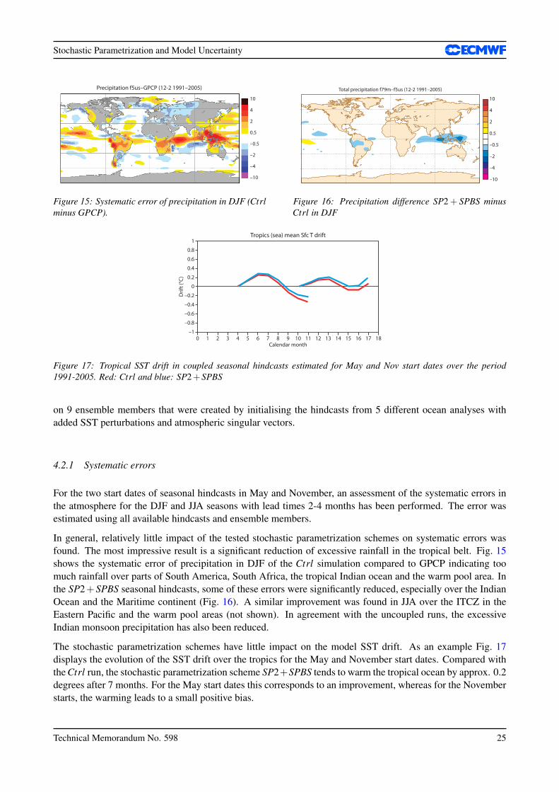
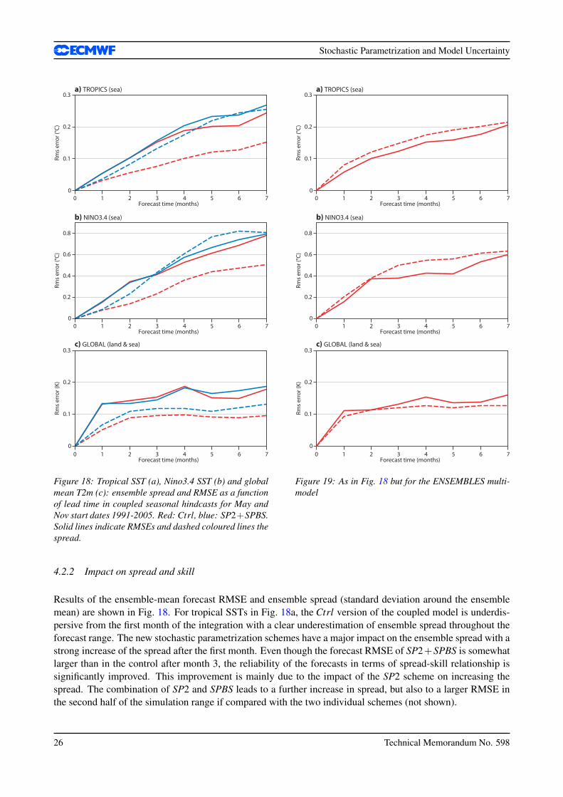
In general, relatively little impact of the tested stochastic parametrization schemes on systematic errors wasfound. The most impressive result is a significant reduction of excessive rainfall in the tropical belt. Fig. 15shows the systematic error of precipitation in DJF of the Ctrl simulation compared to GPCP indicating toomuch rainfall over parts of South America, South Africa, the tropical Indian ocean and the warm pool area. Inthe SP2+SPBS seasonal hindcasts, some of these errors were significantly reduced, especially over the IndianOcean and the Maritime continent (Fig. 16). A similar improvement was found in JJA over the ITCZ in theEastern Pacific and the warm pool areas (not shown). In agreement with the uncoupled runs, the excessiveIndian monsoon precipitation has also been reduced.
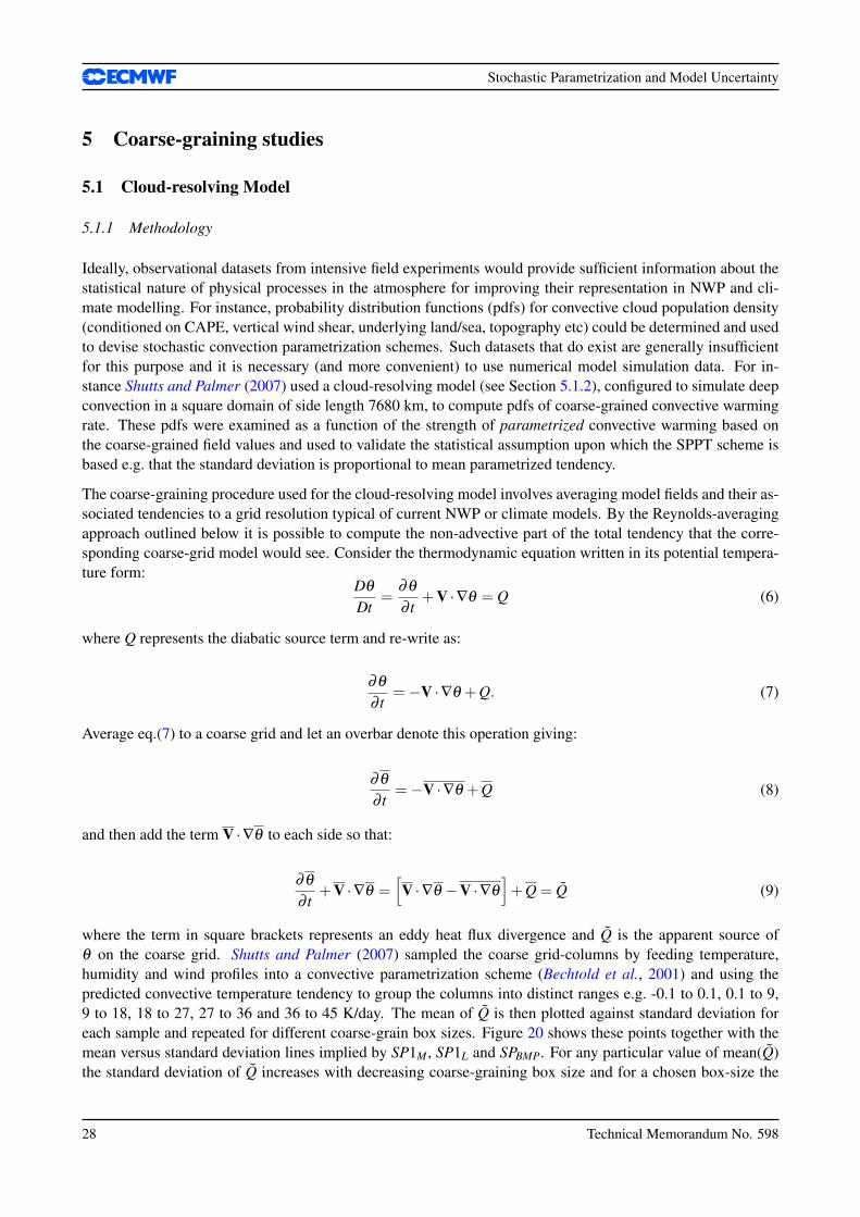
The stochastic parametrization schemes have little impact on the model SST drift. As an example Fig. 17displays the evolution of the SST drift over the tropics for the May and November start dates. Compared withthe Ctrl run, the stochastic parametrization scheme SP2+SPBS tends to warm the tropical ocean by approx. 0.2degrees after 7 months. For the May start dates this corresponds to an improvement, whereas for the Novemberstarts, the warming leads to a small positive bias.
Technical Memorandum No. 598 25
Stochastic Parametrization and Model Uncertainty
Forecast time (months)
0
0.1
0.2
0.3
Rms
erro
r (°C
)
a) TROPICS (sea)
0
0.2
0.4
0.6
0.8
Rms
erro
r (°C
)
b) NINO3.4 (sea)
0
0.1
0.2
0.3
Rms
erro
r (K)
c) GLOBAL (land & sea)
0 1 2 3 4 5 6 7
Forecast time (months)0 1 2 3 4 5 6 7
Forecast time (months)0 1 2 3 4 5 6 7
Figure 18: Tropical SST (a), Nino3.4 SST (b) and globalmean T2m (c): ensemble spread and RMSE as a functionof lead time in coupled seasonal hindcasts for May andNov start dates 1991-2005. Red: Ctrl, blue: SP2+SPBS.Solid lines indicate RMSEs and dashed coloured lines thespread.
Forecast time (months)
0
0.1
0.2
0.3
Rms
erro
r (°C
)
a) TROPICS (sea)
0
0.2
0.4
0.6
0.8
Rms
erro
r (°C
)
b) NINO3.4 (sea)
0
0.1
0.2
0.3
Rms
erro
r (K)
c) GLOBAL (land & sea)
0 1 2 3 4 5 6 7
Forecast time (months)0 1 2 3 4 5 6 7
Forecast time (months)0 1 2 3 4 5 6 7
Figure 19: As in Fig. 18 but for the ENSEMBLES multi-model
4.2.2 Impact on spread and skill
Results of the ensemble-mean forecast RMSE and ensemble spread (standard deviation around the ensemblemean) are shown in Fig. 18. For tropical SSTs in Fig. 18a, the Ctrl version of the coupled model is underdis-persive from the first month of the integration with a clear underestimation of ensemble spread throughout theforecast range. The new stochastic parametrization schemes have a major impact on the ensemble spread with astrong increase of the spread after the first month. Even though the forecast RMSE of SP2+SPBS is somewhatlarger than in the control after month 3, the reliability of the forecasts in terms of spread-skill relationship issignificantly improved. This improvement is mainly due to the impact of the SP2 scheme on increasing thespread. The combination of SP2 and SPBS leads to a further increase in spread, but also to a larger RMSE inthe second half of the simulation range if compared with the two individual schemes (not shown).
26 Technical Memorandum No. 598

Stochastic Parametrization and Model Uncertainty
In the tropical Pacific (Fig. 18b), the increase of ensemble spread due to the new stochastic schemes is evenmore pronounced. Here the forecasts become slightly overdispersive on longer lead times. The increased spreadhas a positive impact on probabilistic forecasts scores that show a higher reliability component of the Brier skillscores than the Ctrl, especially on lead times beyond 3 months (not shown).
The impact of a much increased ensemble spread in SP2+SPBS can also be seen in global mean 2m temperatureforecasts, see Fig. 18c. The spread increases by roughly one quarter over the Ctrl, but is still too small ifcompared with the forecast error. The RMSE in SP2+SPBS remains unchanged vs Ctrl up to forecast month4 and increases slightly beyond that range. The underestimation of ensemble spread is mainly associated withthe oceanic areas (not shown), whereas over land the match between spread and error is, in general, good.
4.2.3 Comparison with the ENSEMBLES multi-model ensemble
We here compare the latest stochastic parametrization results for seasonal forecasting with the multi-modelensemble predictions of the ENSEMBLES project. In ENSEMBLES, 5 coupled climate models from differentinstitutions across Europe have completed a set of 7-month long seasonal hindcasts over the period 1960–2005with 4 start dates per year (Weisheimer et al., 2009).
Fig. 19a shows, similar to Fig. 18a, the evolution of the tropical SST RMSE and ensemble spread for theENSEMBLES multi-model using the same start dates and hindcast period as for the stochastic parametrizationexperiment. While the multi-model ensemble is slightly overdispersive from the first month onwards, theforecast error is smaller than for both Ctrl and SP2+SPBS in Fig. 18a.
Similar conclusions hold for the tropical Pacific SSTs (Fig. 19b). While in the IFS/HOPE coupled system theRMSE continues to grow over lead time, the multi-model ensemble forecast error saturates between months 2and 5 at a level that is below the IFS/HOPE level. Again, the multi-model ensemble is slightly over dispersive.In terms of probabilistic skill scores (not shown), the multi-model ensemble performs, on average, better thanthe Ctrl and the SP2 + SPBS versions of IFS/HOPE. However, for certain events and seasons (upper tercileSST predictions starting in May) the improved reliability components in SP2 + SPBS perform equally well asfor the multi-model ensemble.
Looking at the global scales, the comparison of global mean 2m temperature forecasts between the EN-SEMBLES multi-model ensemble in Fig. 19c and the corresponding figure for IFS/HOPE with stochasticparametrization in Fig. 18c reveals that the multi-model ensemble performs better by generating smaller RM-SEs and a very good match between the ensemble spread and error on all lead times.
Technical Memorandum No. 598 27
Stochastic Parametrization and Model Uncertainty
5 Coarse-graining studies
5.1 Cloud-resolving Model
5.1.1 Methodology
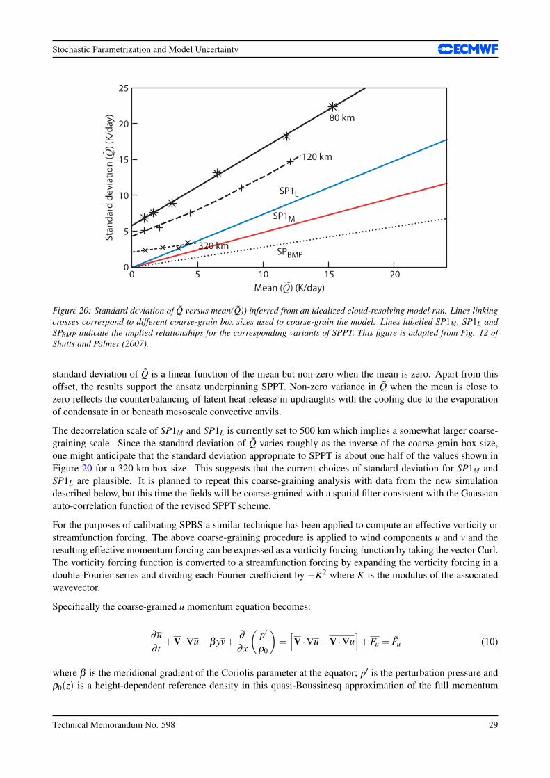
Ideally, observational datasets from intensive field experiments would provide sufficient information about thestatistical nature of physical processes in the atmosphere for improving their representation in NWP and cli-mate modelling. For instance, probability distribution functions (pdfs) for convective cloud population density(conditioned on CAPE, vertical wind shear, underlying land/sea, topography etc) could be determined and usedto devise stochastic convection parametrization schemes. Such datasets that do exist are generally insufficientfor this purpose and it is necessary (and more convenient) to use numerical model simulation data. For in-stance Shutts and Palmer (2007) used a cloud-resolving model (see Section 5.1.2), configured to simulate deepconvection in a square domain of side length 7680 km, to compute pdfs of coarse-grained convective warmingrate. These pdfs were examined as a function of the strength of parametrized convective warming based onthe coarse-grained field values and used to validate the statistical assumption upon which the SPPT scheme isbased e.g. that the standard deviation is proportional to mean parametrized tendency.
The coarse-graining procedure used for the cloud-resolving model involves averaging model fields and their as-sociated tendencies to a grid resolution typical of current NWP or climate models. By the Reynolds-averagingapproach outlined below it is possible to compute the non-advective part of the total tendency that the corre-sponding coarse-grid model would see. Consider the thermodynamic equation written in its potential tempera-ture form:
Dθ
Dt=
∂θ
∂ t+V ·∇θ = Q (6)
where Q represents the diabatic source term and re-write as:
∂θ
∂ t=−V ·∇θ +Q. (7)
Average eq.(7) to a coarse grid and let an overbar denote this operation giving:
∂θ
∂ t=−V ·∇θ +Q (8)
and then add the term V ·∇θ to each side so that:
∂θ
∂ t+V ·∇θ =
[V ·∇θ −V ·∇θ
]+Q = Q (9)
where the term in square brackets represents an eddy heat flux divergence and Q is the apparent source ofθ on the coarse grid. Shutts and Palmer (2007) sampled the coarse grid-columns by feeding temperature,humidity and wind profiles into a convective parametrization scheme (Bechtold et al., 2001) and using thepredicted convective temperature tendency to group the columns into distinct ranges e.g. -0.1 to 0.1, 0.1 to 9,9 to 18, 18 to 27, 27 to 36 and 36 to 45 K/day. The mean of Q is then plotted against standard deviation foreach sample and repeated for different coarse-grain box sizes. Figure 20 shows these points together with themean versus standard deviation lines implied by SP1M, SP1L and SPBMP. For any particular value of mean(Q)the standard deviation of Q increases with decreasing coarse-graining box size and for a chosen box-size the
28 Technical Memorandum No. 598
Stochastic Parametrization and Model Uncertainty
25
20
15
10
5
00 5 10 15 20
80 km
120 km
320 km
SP1L
SP1M
SPBMP
Figure 20: Standard deviation of Q versus mean(Q)) inferred from an idealized cloud-resolving model run. Lines linkingcrosses correspond to different coarse-grain box sizes used to coarse-grain the model. Lines labelled SP1M , SP1L andSPBMP indicate the implied relationships for the corresponding variants of SPPT. This figure is adapted from Fig. 12 ofShutts and Palmer (2007).
standard deviation of Q is a linear function of the mean but non-zero when the mean is zero. Apart from thisoffset, the results support the ansatz underpinning SPPT. Non-zero variance in Q when the mean is close tozero reflects the counterbalancing of latent heat release in updraughts with the cooling due to the evaporationof condensate in or beneath mesoscale convective anvils.
The decorrelation scale of SP1M and SP1L is currently set to 500 km which implies a somewhat larger coarse-graining scale. Since the standard deviation of Q varies roughly as the inverse of the coarse-grain box size,one might anticipate that the standard deviation appropriate to SPPT is about one half of the values shown inFigure 20 for a 320 km box size. This suggests that the current choices of standard deviation for SP1M andSP1L are plausible. It is planned to repeat this coarse-graining analysis with data from the new simulationdescribed below, but this time the fields will be coarse-grained with a spatial filter consistent with the Gaussianauto-correlation function of the revised SPPT scheme.
For the purposes of calibrating SPBS a similar technique has been applied to compute an effective vorticity orstreamfunction forcing. The above coarse-graining procedure is applied to wind components u and v and theresulting effective momentum forcing can be expressed as a vorticity forcing function by taking the vector Curl.The vorticity forcing function is converted to a streamfunction forcing by expanding the vorticity forcing in adouble-Fourier series and dividing each Fourier coefficient by −K2 where K is the modulus of the associatedwavevector.
Specifically the coarse-grained u momentum equation becomes:
∂u∂ t
+V ·∇u−βyv+∂
∂x
(p′
ρ0
)=[V ·∇u−V ·∇u
]+Fu = Fu (10)
where β is the meridional gradient of the Coriolis parameter at the equator; p′ is the perturbation pressure andρ0(z) is a height-dependent reference density in this quasi-Boussinesq approximation of the full momentum
Technical Memorandum No. 598 29
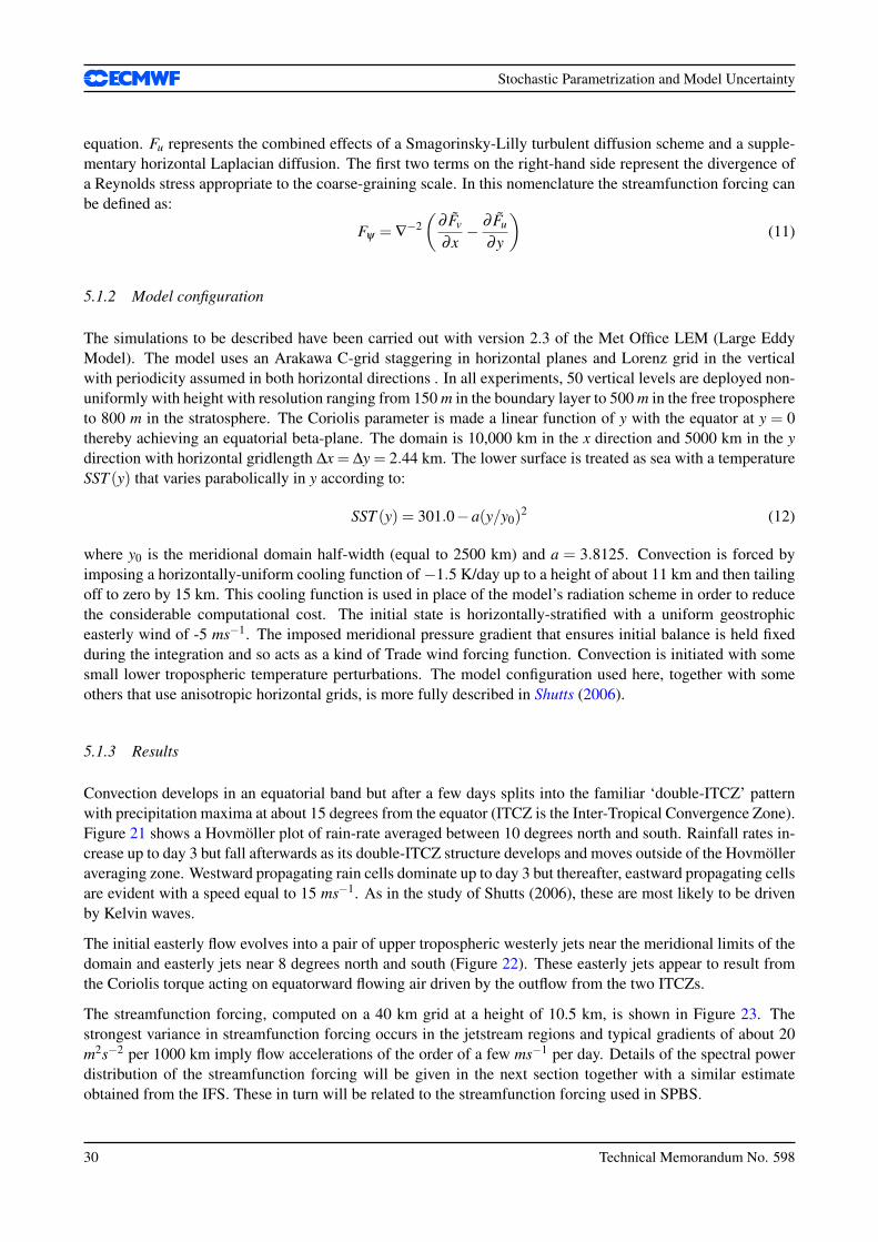
Stochastic Parametrization and Model Uncertainty
equation. Fu represents the combined effects of a Smagorinsky-Lilly turbulent diffusion scheme and a supple-mentary horizontal Laplacian diffusion. The first two terms on the right-hand side represent the divergence ofa Reynolds stress appropriate to the coarse-graining scale. In this nomenclature the streamfunction forcing canbe defined as:
Fψ = ∇−2(
∂ Fv
∂x− ∂ Fu
∂y
)(11)
5.1.2 Model configuration
The simulations to be described have been carried out with version 2.3 of the Met Office LEM (Large EddyModel). The model uses an Arakawa C-grid staggering in horizontal planes and Lorenz grid in the verticalwith periodicity assumed in both horizontal directions . In all experiments, 50 vertical levels are deployed non-uniformly with height with resolution ranging from 150 m in the boundary layer to 500 m in the free troposphereto 800 m in the stratosphere. The Coriolis parameter is made a linear function of y with the equator at y = 0thereby achieving an equatorial beta-plane. The domain is 10,000 km in the x direction and 5000 km in the ydirection with horizontal gridlength ∆x = ∆y = 2.44 km. The lower surface is treated as sea with a temperatureSST (y) that varies parabolically in y according to:
SST (y) = 301.0−a(y/y0)2 (12)
where y0 is the meridional domain half-width (equal to 2500 km) and a = 3.8125. Convection is forced byimposing a horizontally-uniform cooling function of−1.5 K/day up to a height of about 11 km and then tailingoff to zero by 15 km. This cooling function is used in place of the model’s radiation scheme in order to reducethe considerable computational cost. The initial state is horizontally-stratified with a uniform geostrophiceasterly wind of -5 ms−1. The imposed meridional pressure gradient that ensures initial balance is held fixedduring the integration and so acts as a kind of Trade wind forcing function. Convection is initiated with somesmall lower tropospheric temperature perturbations. The model configuration used here, together with someothers that use anisotropic horizontal grids, is more fully described in Shutts (2006).
5.1.3 Results
Convection develops in an equatorial band but after a few days splits into the familiar ‘double-ITCZ’ patternwith precipitation maxima at about 15 degrees from the equator (ITCZ is the Inter-Tropical Convergence Zone).Figure 21 shows a Hovmoller plot of rain-rate averaged between 10 degrees north and south. Rainfall rates in-crease up to day 3 but fall afterwards as its double-ITCZ structure develops and moves outside of the Hovmolleraveraging zone. Westward propagating rain cells dominate up to day 3 but thereafter, eastward propagating cellsare evident with a speed equal to 15 ms−1. As in the study of Shutts (2006), these are most likely to be drivenby Kelvin waves.
The initial easterly flow evolves into a pair of upper tropospheric westerly jets near the meridional limits of thedomain and easterly jets near 8 degrees north and south (Figure 22). These easterly jets appear to result fromthe Coriolis torque acting on equatorward flowing air driven by the outflow from the two ITCZs.
The streamfunction forcing, computed on a 40 km grid at a height of 10.5 km, is shown in Figure 23. Thestrongest variance in streamfunction forcing occurs in the jetstream regions and typical gradients of about 20m2s−2 per 1000 km imply flow accelerations of the order of a few ms−1 per day. Details of the spectral powerdistribution of the streamfunction forcing will be given in the next section together with a similar estimateobtained from the IFS. These in turn will be related to the streamfunction forcing used in SPBS.
30 Technical Memorandum No. 598
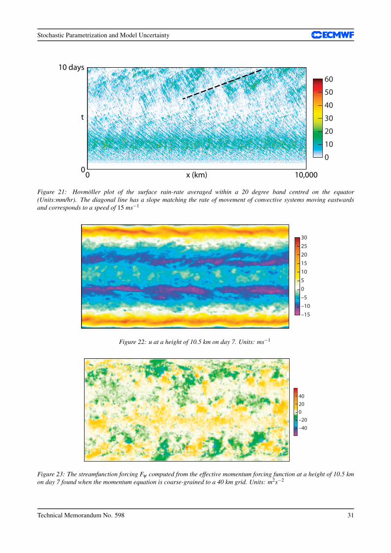
Stochastic Parametrization and Model Uncertainty
10,0000 x (km)
t
0
10 days60
50
40
30
20
10
0
Figure 21: Hovmoller plot of the surface rain-rate averaged within a 20 degree band centred on the equator(Units:mm/hr). The diagonal line has a slope matching the rate of movement of convective systems moving eastwardsand corresponds to a speed of 15 ms−1
302520151050–5–10–15
Figure 22: u at a height of 10.5 km on day 7. Units: ms−1
40200–20–40
Figure 23: The streamfunction forcing Fψ computed from the effective momentum forcing function at a height of 10.5 kmon day 7 found when the momentum equation is coarse-grained to a 40 km grid. Units: m2s−2
Technical Memorandum No. 598 31
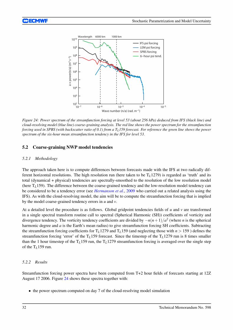
Stochastic Parametrization and Model Uncertainty
102
103
104
105
106
107
108
109
1010
10−7 10−6 10−5 10–4 10–3
a ×
pow
er(n
/a) (
m3 s
−2)
Wave number (n/a) (rad. m−1)
IFS psi forcing LEM psi forcing SPBS forcing6−hour psi tend.
1000 km6000 kmWavelength
Figure 24: Power spectrum of the streamfunction forcing at level 53 (about 256 hPa) deduced from IFS (black line) andcloud-resolving model (blue line) coarse-graining analysis. The red line shows the power spectrum for the streamfunctionforcing used in SPBS (with backscatter ratio of 0.1) from a TL159 forecast. For reference the green line shows the powerspectrum of the six-hour mean streamfunction tendency in the IFS for level 53.
5.2 Coarse-graining NWP model tendencies
5.2.1 Methodology
The approach taken here is to compute differences between forecasts made with the IFS at two radically dif-ferent horizontal resolutions. The high resolution run (here taken to be TL1279) is regarded as ‘truth’ and itstotal (dynamical + physical) tendencies are spectrally-smoothed to the resolution of the low resolution model(here TL159). The difference between the coarse-grained tendency and the low-resolution model tendency canbe considered to be a tendency error (see Hermanson et al., 2009 who carried out a related analysis using theIFS). As with the cloud-resolving model, the aim will be to compute the streamfunction forcing that is impliedby the model coarse-grained tendency errors in u and v.
At a detailed level the procedure is as follows. Global gridpoint tendencies fields of u and v are transformedin a single spectral transform routine call to spectral (Spherical Harmonic (SH)) coefficients of vorticity anddivergence tendency. The vorticity tendency coefficients are divided by −n(n+1)/a2 (where n is the sphericalharmonic degree and a is the Earth’s mean radius) to give streamfunction forcing SH coefficients. Subtractingthe streamfunction forcing coefficients for TL1279 and TL159 (and neglecting those with n > 159 ) defines thestreamfunction forcing ‘error’ of the TL159 forecast. Since the timestep of the TL1279 run is 8 times smallerthan the 1 hour timestep of the TL159 run, the TL1279 streamfunction forcing is averaged over the single stepof the TL159 run.
5.2.2 Results
Streamfunction forcing power spectra have been computed from T+2 hour fields of forecasts starting at 12ZAugust 17 2006. Figure 24 shows these spectra together with:
• the power spectrum computed on day 7 of the cloud-resolving model simulation
32 Technical Memorandum No. 598
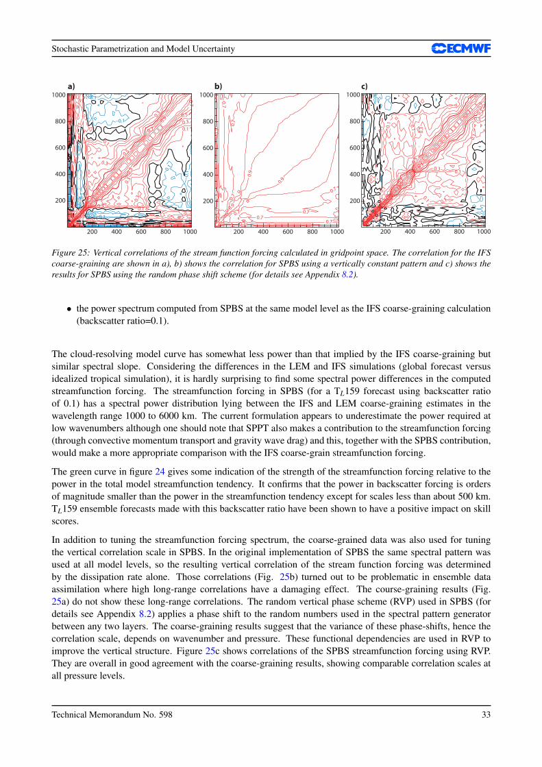
Stochastic Parametrization and Model Uncertainty
200 400 600 800 1000
200
400
600
800
1000
0.1
0.1
0.1
0.1
0.1 0.
1
0.1
0.1
0.3
0.3
0.3
0.3
0.5
0.5
0.5
0.7
0.7
0.7
200 400 600 800 1000
200
400
600
800
1000
200 400 600 800 1000
200
400
600
800
1000
−0.1
−0.1
−0.1
−0.1
−0.1
−0.1
0.1
0.1
0.1
0.1
0.1
0.1
0.30.
3
0.3
0.3
0.3
0.3
0.5
0.50.5
0.7
0.7
0.7
0.9
a) b) c)
0.5
0.5
0.5
0.70.7
0.7
0.70.7
0.7
0.7
0.7
0.9
0.9
0.9
Figure 25: Vertical correlations of the stream function forcing calculated in gridpoint space. The correlation for the IFScoarse-graining are shown in a), b) shows the correlation for SPBS using a vertically constant pattern and c) shows theresults for SPBS using the random phase shift scheme (for details see Appendix 8.2).
• the power spectrum computed from SPBS at the same model level as the IFS coarse-graining calculation(backscatter ratio=0.1).
The cloud-resolving model curve has somewhat less power than that implied by the IFS coarse-graining butsimilar spectral slope. Considering the differences in the LEM and IFS simulations (global forecast versusidealized tropical simulation), it is hardly surprising to find some spectral power differences in the computedstreamfunction forcing. The streamfunction forcing in SPBS (for a TL159 forecast using backscatter ratioof 0.1) has a spectral power distribution lying between the IFS and LEM coarse-graining estimates in thewavelength range 1000 to 6000 km. The current formulation appears to underestimate the power required atlow wavenumbers although one should note that SPPT also makes a contribution to the streamfunction forcing(through convective momentum transport and gravity wave drag) and this, together with the SPBS contribution,would make a more appropriate comparison with the IFS coarse-grain streamfunction forcing.
The green curve in figure 24 gives some indication of the strength of the streamfunction forcing relative to thepower in the total model streamfunction tendency. It confirms that the power in backscatter forcing is ordersof magnitude smaller than the power in the streamfunction tendency except for scales less than about 500 km.TL159 ensemble forecasts made with this backscatter ratio have been shown to have a positive impact on skillscores.
In addition to tuning the streamfunction forcing spectrum, the coarse-grained data was also used for tuningthe vertical correlation scale in SPBS. In the original implementation of SPBS the same spectral pattern wasused at all model levels, so the resulting vertical correlation of the stream function forcing was determinedby the dissipation rate alone. Those correlations (Fig. 25b) turned out to be problematic in ensemble dataassimilation where high long-range correlations have a damaging effect. The course-graining results (Fig.25a) do not show these long-range correlations. The random vertical phase scheme (RVP) used in SPBS (fordetails see Appendix 8.2) applies a phase shift to the random numbers used in the spectral pattern generatorbetween any two layers. The coarse-graining results suggest that the variance of these phase-shifts, hence thecorrelation scale, depends on wavenumber and pressure. These functional dependencies are used in RVP toimprove the vertical structure. Figure 25c shows correlations of the SPBS streamfunction forcing using RVP.They are overall in good agreement with the coarse-graining results, showing comparable correlation scales atall pressure levels.
Technical Memorandum No. 598 33
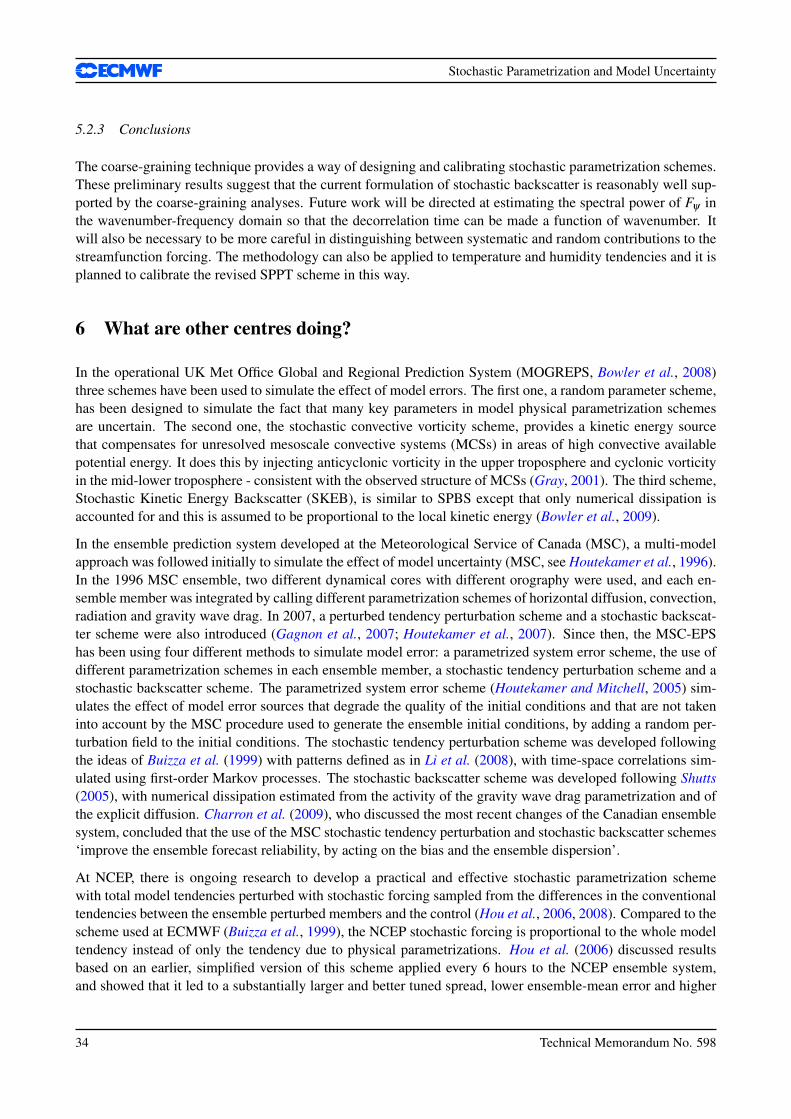
Stochastic Parametrization and Model Uncertainty
5.2.3 Conclusions
The coarse-graining technique provides a way of designing and calibrating stochastic parametrization schemes.These preliminary results suggest that the current formulation of stochastic backscatter is reasonably well sup-ported by the coarse-graining analyses. Future work will be directed at estimating the spectral power of Fψ inthe wavenumber-frequency domain so that the decorrelation time can be made a function of wavenumber. Itwill also be necessary to be more careful in distinguishing between systematic and random contributions to thestreamfunction forcing. The methodology can also be applied to temperature and humidity tendencies and it isplanned to calibrate the revised SPPT scheme in this way.
6 What are other centres doing?
In the operational UK Met Office Global and Regional Prediction System (MOGREPS, Bowler et al., 2008)three schemes have been used to simulate the effect of model errors. The first one, a random parameter scheme,has been designed to simulate the fact that many key parameters in model physical parametrization schemesare uncertain. The second one, the stochastic convective vorticity scheme, provides a kinetic energy sourcethat compensates for unresolved mesoscale convective systems (MCSs) in areas of high convective availablepotential energy. It does this by injecting anticyclonic vorticity in the upper troposphere and cyclonic vorticityin the mid-lower troposphere - consistent with the observed structure of MCSs (Gray, 2001). The third scheme,Stochastic Kinetic Energy Backscatter (SKEB), is similar to SPBS except that only numerical dissipation isaccounted for and this is assumed to be proportional to the local kinetic energy (Bowler et al., 2009).
In the ensemble prediction system developed at the Meteorological Service of Canada (MSC), a multi-modelapproach was followed initially to simulate the effect of model uncertainty (MSC, see Houtekamer et al., 1996).In the 1996 MSC ensemble, two different dynamical cores with different orography were used, and each en-semble member was integrated by calling different parametrization schemes of horizontal diffusion, convection,radiation and gravity wave drag. In 2007, a perturbed tendency perturbation scheme and a stochastic backscat-ter scheme were also introduced (Gagnon et al., 2007; Houtekamer et al., 2007). Since then, the MSC-EPShas been using four different methods to simulate model error: a parametrized system error scheme, the use ofdifferent parametrization schemes in each ensemble member, a stochastic tendency perturbation scheme and astochastic backscatter scheme. The parametrized system error scheme (Houtekamer and Mitchell, 2005) sim-ulates the effect of model error sources that degrade the quality of the initial conditions and that are not takeninto account by the MSC procedure used to generate the ensemble initial conditions, by adding a random per-turbation field to the initial conditions. The stochastic tendency perturbation scheme was developed followingthe ideas of Buizza et al. (1999) with patterns defined as in Li et al. (2008), with time-space correlations sim-ulated using first-order Markov processes. The stochastic backscatter scheme was developed following Shutts(2005), with numerical dissipation estimated from the activity of the gravity wave drag parametrization and ofthe explicit diffusion. Charron et al. (2009), who discussed the most recent changes of the Canadian ensemblesystem, concluded that the use of the MSC stochastic tendency perturbation and stochastic backscatter schemes‘improve the ensemble forecast reliability, by acting on the bias and the ensemble dispersion’.
At NCEP, there is ongoing research to develop a practical and effective stochastic parametrization schemewith total model tendencies perturbed with stochastic forcing sampled from the differences in the conventionaltendencies between the ensemble perturbed members and the control (Hou et al., 2006, 2008). Compared to thescheme used at ECMWF (Buizza et al., 1999), the NCEP stochastic forcing is proportional to the whole modeltendency instead of only the tendency due to physical parametrizations. Hou et al. (2006) discussed resultsbased on an earlier, simplified version of this scheme applied every 6 hours to the NCEP ensemble system,and showed that it led to a substantially larger and better tuned spread, lower ensemble-mean error and higher
34 Technical Memorandum No. 598
Stochastic Parametrization and Model Uncertainty
probabilistic scores. More recent results (Hou et al., 2008) indicated that a refined version of the scheme cansignificantly improve the performance of the NCEP ensemble system.
In the US Navy Operational Global Atmospheric Prediction System (NOGAPS) ensemble system, a ‘stochasticconvection’ approach (Teixeira and Reynolds, 2008) is used to simulate model error uncertainties mainly due toconvection parametrization. Within this approach, parametrization schemes are used with control parameterssampled from a distribution of probable values instead of with a unique, most likely value. They showed thatthis approach led to a substantial increase of the NOGAPS ensemble spread in the tropics, and a small increasein the extra-tropics, with positive impacts on some measurements of ensemble forecast skill. Reynolds et al.(2008) showed that the use of this scheme helps to mitigate a fundamental problem, namely, that ensemblesystems with initial conditions defined using Ensemble Transformed methods have too little initial variance inthe tropics and too much variance in the extra-tropics.
7 Conclusions and Discussion
Two complementary stochastic parametrization schemes have been developed and their impacts have beenstudied on medium-range and seasonal forecast timescales.
Research will continue to develop and extend these stochastic parametrizations. For example, results for theseasonal predictions indicate that, despite SPPT and SPBS, the EPS remains underdispersive for 2m temper-ature. This may indicate that a stochastic element should be included in the land surface component of theforecast model. However, more likely, such underdispersion suggests that variables associated with cloudamount should be treated stochastically. Work to extend the stochastic parametrizations in this direction willbegin shortly.
Currently, the stochastic parametrizations discussed in this paper are applied only to the atmospheric model.However, there is no reason in principle why they should be so restricted, and further developments should seestochastic parametrization schemes being applied to the land and oceanic components of the ECMWF forecastsystem.
Both stochastic schemes discussed in Section 2 use spectral stochastic pattern generators. There are otherschemes which allow one to focus on spatially confined features of the flow. For example, Palmer (1997,2001) suggested the use of stochastic cellular automata as providing pattern generators to represent individualmesoscale convective complexes. Early results using a cellular automaton pattern generator in seasonal forecastmode have been promising (Berner et al., 2008). There are some advantages to such cellular automata schemes.For example, it is straightforward to represent the advection of a convective complex by some steering levelflow. In this way, information about convective instability can propagate from one grid box to a neighbouringone, in a way which a conventional convective parametrization cannot do. It is possible that the representationof advection of convective systems by the trade winds may be an important process missing in conventionalschemes, for the correct development of the Madden-Julian Oscillation and research is underway to test this.
Ultimately, stochastic representations should be incorporated ab initio into the development of parametrizationschemes; the schemes described in Section 2 are essentially “bolt on” extras, to be added to standard determin-istic parametrization schemes. An example of an approach where a parametrization is considered stochastic abinitio is the scheme developed by Plant and Craig (2008), where one assumes a statistical ensemble of convec-tive plumes with inherently small sample size, leading to significant dispersion of some underlying probabilitydistribution.
As discussed in the text, very high resolution cloud-resolving models provide a rigorous approach to the devel-opment of stochastic parametrization and will become an increasingly important tool for the future.
Technical Memorandum No. 598 35
Stochastic Parametrization and Model Uncertainty
This paper has focused on the application of stochastic parametrization on prediction timescales from themedium range to the seasonal. However, on the basis that insights and constraints on these timescales caninform prediction on longer timescales where verification data does not yet exist - the seamless predictionparadigm - it would seem reasonable to conjecture that stochastic parametrization should play a key role inthe development of Earth System Models for multi-decadal and centennial climate prediction. Indeed since anEarth System Model purports to be a comprehensive representation of processes and aspects needed to pre-dict climate, it should by definition be capable of predicting uncertainty. Currently, individual Earth SystemModels are not so capable, and standard ways of predicting uncertainty (e.g. in IPCC assessment reports) makeuse of the multi-model ensemble. Additionally, as discussed in the context of seasonal prediction timescales,stochastic parametrizations can reduce systematic biases, and therefore in some sense could be considered a“poor man’s” alternative to higher resolution. This consideration may be particularly important when limitedcomputer resources are needed to represent biogeochemistry, the dynamic cryosphere, and other aspects ofEarth-System complexity. It seems reasonable therefore to propose that next-generation Earth System Modelsshould be explicitly stochastic (Palmer et al., 2009).
8 Appendix
8.1 Stochastically Perturbed Parametrization Tendencies
Now, the details of the pattern generator for the multiplicative noise used in the revised stochastically perturbedparametrization tendencies scheme are described. Let r denote, as before, the pattern in grid point space and rits spectral transform, i.e.
r = ∑mn
rmnYmn, (13)
where Ymn, m and n denote a spherical harmonic, the zonal wavenumber and the total wavenumber, respectively.The spectral coefficients rmn ∈ C evolve according to an AR(1) process
rmn(t +∆t) = φ rmn(t)+σnηmn(t), (14)
where the ηmn ∈ C denote random numbers. Real part and imaginary part of ηmn are independent Gaussianrandom numbers with unit variance and zero mean. Furthermore, ηmn are also independent for different spher-ical harmonics and white in time. The temporal correlation of rmn is controlled by φ , which is the correlationover one timestep ∆t. Given a decorrelation timescale τ , the one-timestep correlation is set to
φ = exp(−∆t/τ). (15)
The variance of rmn depends on the one-timestep correlation according to
var(Re rmn) = var(Im rmn) =σ2
n
1−φ 2 . (16)
The standard deviation in (14) is set to
σn = F0 exp(−κT n(n+1)/2) with (17)
F0 =
(var(r)
(1−φ 2
)2∑
Nn=1(2n+1)exp(−κT n(n+1))
)1/2
(18)
36 Technical Memorandum No. 598
Stochastic Parametrization and Model Uncertainty
The choice of the normalisation factor F0 ensures that the variance at any point on the sphere is given by var(r)as the variance in grid point space is uniform and equals the total variance in spectral space.
The variance spectrum of rmn depends on total wavenumber as exp(−κT n(n+1)), where parameter κT deter-mines the horizontal correlation length. Therefore, the pattern has a spatial autocorrelation corresponding tothe equivalent of a Gaussian on the sphere according to Weaver and Courtier (2001). The correlation lengthscale is approximately given by (2κT )1/2RE , where RE denotes the earth’s radius.
At initial time, the spectral random numbers are initialised by
rmn(0) = (1−φ2)−1/2
σnηmn(0). (19)
Thus, a statistically steady state is achieved immediately without having to spin up the AR(1) processes.
In order to avoid arithmetic overflow, the random numbers ηmn and the spectral coefficients rmn are bounded tothe range of ±10 standard deviations. This has no practical impact on the distribution but makes the code nu-merically safe. Furthermore, the pattern is bounded in grid point space in order to avoid numerical instabilities.The range is limited to ±3 standard deviations for SP1M and to ±2 standard deviations for SP1L.
8.2 Stochastic backscatter
The streamfunction forcing (Fψ ) is defined to be the product of a pattern field and the square root of a totaldissipation rate function (Dtot). The pattern field evolves in time and contains information about the powerspectrum of the forcing with the dissipation rate factor acting as an amplitude modulator. The horizontalstructure of the pattern field (Fψ∗) is represented by:
F jψ∗,k =
N
∑m=−N
N
∑n=|m|
f jm,n,kP|m|n (µ) exp(imλ ) (20)
where m is the zonal wavenumber, n is the degree of the associated Legendre function Pmn (µ), f j
m,n,k is thespectral coefficient satisfying the reality condition
f jm,n,k = f j∗
−m,n,k
where the superscript ∗ denotes the complex conjugate , µ is the sine of the latitude, λ is the longitude, k is themodel level number and j is the number of timesteps of length ∆t. This series expansion represents a triangularspectral truncation at spherical harmonic degree N. The time evolution of the spectral coefficients f j
m,n,k isassumed to be governed by a first-order auto-regressive process defined by:
f j+1m,n,k = [1−α(n)] f j
m,n,k +√
α(n)g(n)r jm,n,k (21)
where α(n) is a wavenumber-dependent parameter lying between 0 (no stochastic forcing) and 1 (white noiseforcing); g(n) is a real function controlling the spectral power in each mode and r j
m,n,k = a jm,n,k + ib j
m,n,k where
a jm,n,k and b j
m,n,k are random numbers with zero mean and variance Σ2. Therefore, each spherical harmonicmode, characterized by (m,n), is associated with a discrete time series of complex random numbers indexed byj. Inspection of the ‘memory term’ in equation (21) suggests the definition α(n) = 1− exp(−∆t/τ(n)) whereτ(n) is a exponential time scale. In general the decorrelation time should be dependent on spatial scale and soallowance is made for that in the definition of τ .
Technical Memorandum No. 598 37
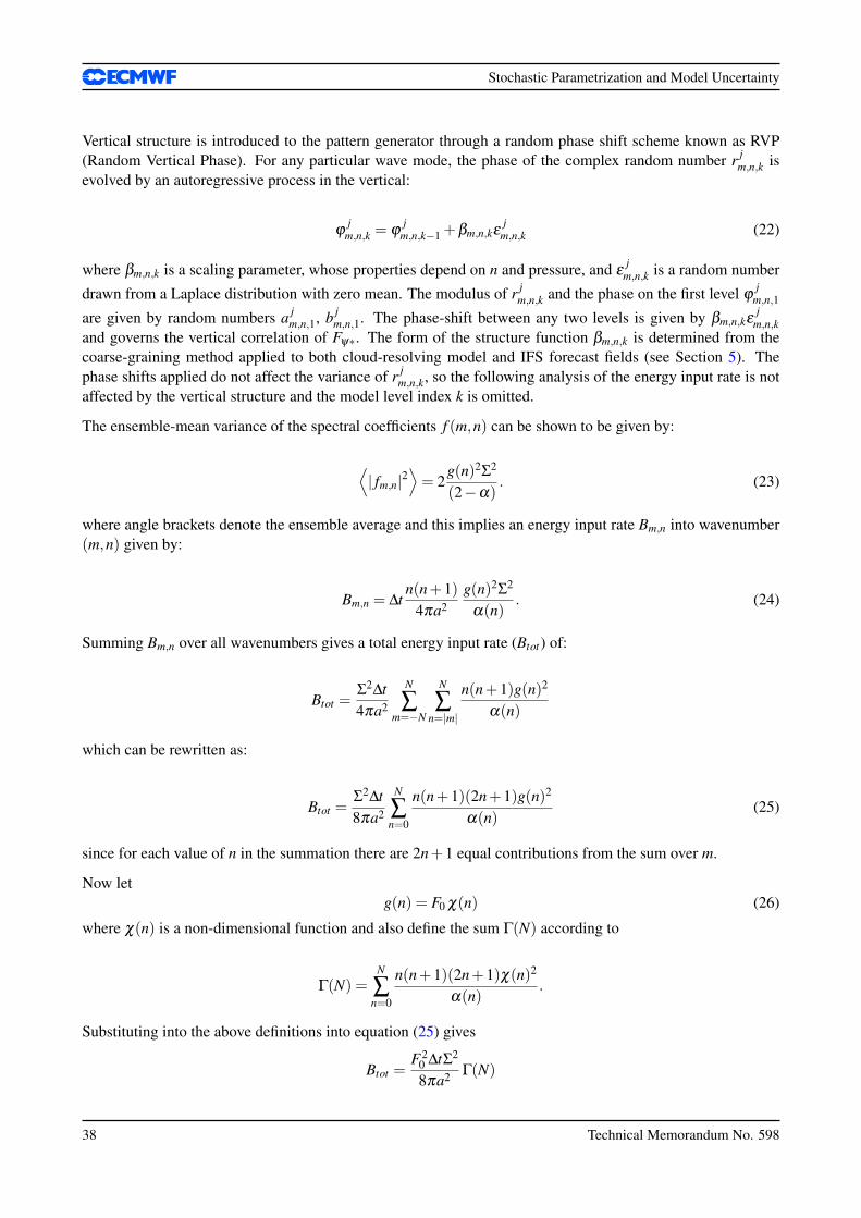
Stochastic Parametrization and Model Uncertainty
Vertical structure is introduced to the pattern generator through a random phase shift scheme known as RVP(Random Vertical Phase). For any particular wave mode, the phase of the complex random number r j
m,n,k isevolved by an autoregressive process in the vertical:
ϕj
m,n,k = ϕj
m,n,k−1 +βm,n,kεj
m,n,k (22)
where βm,n,k is a scaling parameter, whose properties depend on n and pressure, and εj
m,n,k is a random number
drawn from a Laplace distribution with zero mean. The modulus of r jm,n,k and the phase on the first level ϕ
jm,n,1
are given by random numbers a jm,n,1, b j
m,n,1. The phase-shift between any two levels is given by βm,n,kεj
m,n,kand governs the vertical correlation of Fψ∗. The form of the structure function βm,n,k is determined from thecoarse-graining method applied to both cloud-resolving model and IFS forecast fields (see Section 5). Thephase shifts applied do not affect the variance of r j
m,n,k, so the following analysis of the energy input rate is notaffected by the vertical structure and the model level index k is omitted.
The ensemble-mean variance of the spectral coefficients f (m,n) can be shown to be given by:
⟨| fm,n|2
⟩= 2
g(n)2Σ2
(2−α). (23)
where angle brackets denote the ensemble average and this implies an energy input rate Bm,n into wavenumber(m,n) given by:
Bm,n = ∆tn(n+1)
4πa2g(n)2Σ2
α(n). (24)
Summing Bm,n over all wavenumbers gives a total energy input rate (Btot) of:
Btot =Σ2∆t4πa2
N
∑m=−N
N
∑n=|m|
n(n+1)g(n)2
α(n)
which can be rewritten as:
Btot =Σ2∆t8πa2
N
∑n=0
n(n+1)(2n+1)g(n)2
α(n)(25)
since for each value of n in the summation there are 2n+1 equal contributions from the sum over m.
Now letg(n) = F0 χ(n) (26)
where χ(n) is a non-dimensional function and also define the sum Γ(N) according to
Γ(N) =N
∑n=0
n(n+1)(2n+1)χ(n)2
α(n).
Substituting into the above definitions into equation (25) gives
Btot =F2
0 ∆tΣ2
8πa2 Γ(N)
38 Technical Memorandum No. 598
Stochastic Parametrization and Model Uncertainty
which on rearranging for F0 gives:
F0 =(
8πa2Btot
∆t Γ(N)Σ2
)1/2
. (27)
The coarse-graining studies to be discussed in Section 5 suggest that χ(n) may behave like a power law forlarge n and our current implementation assumes:
χ(n) = (1+n)−1.27. (28)
Therefore the energy input rate can be controlled through F0 and equated to a diagnosed total dissipation ratemultiplied by a backscatter ratio bR. The full streamfunction forcing is therefore given by:
Fψ =(
bRDtot
Btot
)1/2
Fψ∗ (29)
which expresses the fact that if Fψ∗ gives an energy input rate of Btot per unit mass then Fψ gives an energyinput rate of bRDtot i.e. a fraction bR of the total dissipation rate Dtot .
Acknowledgements.
We are grateful to several people that contributed to this work through discussions, diagnostics or numericalexperimentation: Michael Ball, Peter Bechtold, Anton Beljaars, Judith Berner, Lars Isaksen, Philippe Lopez,Martin Miller, Franco Molteni, Mark Rodwell, Frederic Vitart.
References
Barkmeijer, J., R. Buizza, and T. N. Palmer (1999), 3D-Var Hessian singular vectors and their potential use inthe ECMWF Ensemble Prediction System, Quart. J. Roy. Meteorol. Soc., 125, 2333–2351.
Bechtold, P., E. Bazile, F. Guichard, P. Mascart, and E. Richard (2001), A mass flux convection scheme forregional and global models., Q.J.R.Meteorol.Soc., 127, 869–886.
Berner, J., F. Doblas-Reyes, T. N. Palmer, G. J. Shutts, and A. Weisheimer (2008), Impact of a quasi-stochasticcellular automaton backscatter scheme on the systematic error and seasonal prediction skill of a global cli-mate model., Phil. Trans. R. Soc. A, 366, 2561–2579, doi:10.1098/rsta.2008.0033.
Berner, J., T. Jung, and T. N. Palmer (2009a), Influence of stochastic parametrization versus horizontal resolu-tion on systematic model error, manuscript in preparation.
Berner, J., G. J. Shutts, M. Leutbecher, and T. N. Palmer (2009b), A spectral stochastic kinetic energy backscat-ter scheme and its impact on flow-dependent predictability in the ECMWF ensemble prediction system, J.Atmos. Sci., 66, 603–626.
Bormann, N., S. Saarinen, G. Kelly, and J. N. Thepaut (2003), The spatial structure of observation errors inatmospheric motion vectors from geostationary satellite data, Mon. Weather Rev., 131, 706–718.
Bowler, N. E., A. Arribas, K. R. Mylne, K. B. Robertson, and S. E. Beare (2008), The MOGREPS short-rangeensemble prediction system, Quart. J. Roy. Meteorol. Soc., 134, 703–722.
Technical Memorandum No. 598 39
Stochastic Parametrization and Model Uncertainty
Bowler, N. E., A. Arribas, S. E. Beare, K. R. Mylne, and G. J. Shutts (2009), The local ETKF and SKEB:Upgrade to the MOGREPS short-range ensemble prediction system, Quart. J. Roy. Meteorol. Soc., 135,767–776.
Buizza, R., and T. N. Palmer (1995), The singular-vector structure of the atmospheric general circulation, J.Atmos. Sci., 52, 1434–1456.
Buizza, R., M. Miller, and T. N. Palmer (1999), Stochastic representation of model uncertainties in the ECMWFEnsemble Prediction System, Quart. J. Roy. Meteorol. Soc., 125, 2887–2908.
Buizza, R., M. Leutbecher, and L. Isaksen (2008), Potential use of an ensemble of analyses in the ECMWFEnsemble Prediction System, Quart. J. Roy. Meteorol. Soc., 134, 2051–2066.
Charron, M., G. Pellerin, L. Spacek, P. L. Houtekamer, N. Gagnon, H. L. Mitchell, and L. Michelin (2009),The Canadian global ensemble prediction system with a single dynamical core and stochastic physical per-turbations, submitted to Mon. Weather Rev.
Doblas-Reyes, F., A. Weisheimer, M. Deque, N. Keenlyside, M. McVean, J. M. Murphy, P. Rogel, D. Smith, andT. N. Palmer (2009), Addressing model uncertainty in seasonal and annual dynamical ensemble forecasts.,Quart. J. Roy. Meteorol. Soc., 135(643), 1538–1559.
Evans, R. E., R. J. Graham, M. S. J. Harrison, and G. J. Shutts (1998), Preliminary investigations into the effectof adding stochastic backscatter to the Unified Model, Met Office Forecasting Research Technical Report,No. 241, Met Office, Exeter, UK.
Frederiksen, J. S., and A. G. Davies (1997), Eddy viscosity and stochastic backscatter parameterizations on thesphere for atmospheric circulation models., J. Atmos. Sci., 54, 2475–2492.
Gagnon, N., G. Pellerin, M. Charron, P. Houtekamer, H. Mitchell, G. Candille, L. Spacek, X.-X. Deng, B. He,and R. Verret (2007), An update on the CMC ensemble medium-range forecast system, in Proceedings ofthe ECMWF 11th Workshop on Meteorological Operational Systems, 12-16 November 2007, pp. 55–59,ECMWF, Shinfield Park, Reading, Berkshire RG2 9AX, UK.
Gray, M. E. B. (2001), The impact of mesoscale convective-system potential-vorticity anomalies on numerical-weather-prediction forecasts, Q. J. R. Meteorol. Soc., 127, 73–88.
Hermanson, L., B. J. Hoskins, and T. N. Palmer (2009), A comparative method to evaluate and validate stochas-tic parametrizations, Q. J. R. Meteorol. Soc., 135, 10.1002/qj.436.
Hou, D., Z. Toth, and Y. Zhu (2006), A stochastic parameterisation scheme within NCEP global ensembleforecast system, in Proceedings of the 18th AMS Conference on Probability and Statistics, 29 January - 2February 2006, Atlanta, GA.
Hou, D., Z. Toth, Y. Zhu, and W. Yang (2008), Impact of a stochastic perturbation scheme on NCEP globalensemble forecast system, in Proceedings of the 19th AMS Conference on Probability and Statistics, 21-24January 2008, New Orleans, Louisiana.
Houtekamer, P. L., and H. L. Mitchell (2005), Ensemble Kalman filtering, Quart. J. Roy. Meteorol. Soc., 131,3269–3289.
Houtekamer, P. L., L. Lefaivre, J. Derome, H. Ritchie, and H. L. Mitchell (1996), A system simulation approachto ensemble prediction, Mon. Weather Rev., 124, 1225–1242.
40 Technical Memorandum No. 598
Stochastic Parametrization and Model Uncertainty
Houtekamer, P. L., M. Charron, H. L. Mitchell, and G. Pellerin (2007), Status of the global EPS at EnvironmentCanada, in Proceedings of the ECMWF Workshop on Ensemble Prediction, 7-9 November 2007, pp. 57–68,ECMWF, Shinfield Park, Reading, Berkshire RG2 9AX, UK.
Isaksen, L., M. Fisher, and J. Berner (2007), Use of analysis ensembles in estimating flow-dependent back-ground error variance, in ECMWF Workshop on ”Flow-dependent aspects of data assimilation”, 11-13 June2007, pp. 65–86, ECMWF, Shinfield Park, Reading, Berkshire RG2 9AX, UK.
Jung, T., T. N. Palmer, and G. J. Shutts (2005), Influence of a stochastic parameterization on the frequencyof occurrence of North Pacific weather regimes in the ECMWF model, Geophys. Res. Lett., 32, L23,811,doi:10.1029/2005GL024248.
Jung, T., G. Balsamo, P. Bechtold, A. Beljaars, M. Kohler, M. Miller, J.-J. Morcrette, A. Orr, M. J. Rodwell,and A. M. Tompkins (2009), The ECMWF model climate: Recent progress through improved physicalparametrizations, in Proceedings of ECMWF Seminar on Parametrization of Subgrid Physical Processes,pp. 233–250, ECMWF, Shinfield Park, Reading, Berkshire RG2 9AX, UK.
Leutbecher, M., and T. N. Palmer (2008), Ensemble forecasting, J. Comp. Phys., 227, 3515–3539.
Li, X., M. Charron, L. Spacek, and G. Candille (2008), A regional ensemble prediction system based on moisttargeted singular vectors and stochastic parameter perturbations, Mon. Weather Rev., 136, 443–462.
Mason, P. J., and D. J. Thomson (1992), Stochastic backscatter in large-eddy simulations of boundary layers.,J. Fluid Mech., 242, 51–78.
Palmer, T. N. (1997), On parametrizing scales that are only somewhat smaller than the smallest resolved scales,with application to convection and orography, in Proceedings of the ECMWF Workshop on New Insightsand Approaches to Convective Parametrization, 4-7 November 1996, pp. 328–337, ECMWF, Shinfield Park,Reading, Berkshire RG2 9AX, UK.
Palmer, T. N. (2001), A nonlinear dynamical perspective on model error: A proposal for non-local stochastic-dynamic parametrization in weather and climate prediction models, Q. J. R. Meteorol. Soc., 127, 279–304.
Palmer, T. N., R. Gelaro, J. Barkmeijer, and R. Buizza (1998), Singular vectors, metrics, and adaptive observa-tions, J. Atmos. Sci., 55, 633–653.
Palmer, T. N., A. Alessandri, U. Andersen, P. Cantelaube, M. Davey, P. Delecluse, M. Deque, E. Dıez, F. J.Doblas-Reyes, H. Feddersen, R. Graham, S. Gualdi, J. F. Gueremy, R. Hagedorn, M. Hoshen, N. Keenlyside,M. Latif, A. Lazar, E. Maisonnave, V. Marletto, A. P. Morse, B. Orfila, P. Rogel, J. M. Terres, and M. C.Thomson (2004), Development of a european multimodel ensemble system for seasonal-to-interannual pre-diction (demeter), Bull. Amer. Meteor. Soc., 85, 853–872.
Palmer, T. N., G. J. Shutts, R. Hagedorn, F. Doblas-Reyes, T. Jung, and M. Leutbecher (2005), Representingmodel uncertainty in weather and climate prediction, Ann. Rev. Earth Planet. Sci., 33, 163–193.
Palmer, T. N., F.-J. Doblas-Reyes, A. Weisheimer, G. J. Shutts, J. Berner, and J. M. Murphy (2009), Towardsthe Probabilistic Earth-System Model, arxiv.org: 0812.1074.
Plant, R. S., and G. C. Craig (2008), A stochastic parameterization for deep convection based on equilibriumstatistics, J. Atmos. Sci., 65, 87–105.
Reynolds, C. A., J. Teixeira, and J. G. McLay (2008), Impact of stochastic convection on the Ensemble Trans-form, Notes and Correspondences of Mon. Wea. Rev., 136, 4517–4526.
Technical Memorandum No. 598 41
Stochastic Parametrization and Model Uncertainty
Rodwell, M. J., and T. Jung (2008), The ECMWF ‘Diagnostic Explorer’: A web tool to aid forecast systemassessment and development, ECMWF Newsletter 117, ECMWF, Shinfield Park, Reading, Berkshire RG29AX, UK.
Shutts, G. J. (2005), A kinetic energy backscatter algorithm for use in ensemble prediction systems, Q. J. R.Meteorol. Soc., 131, 3079–3102.
Shutts, G. J. (2006), Upscale effects in simulations of tropical convection on an equatorial beta-plane, DynamicsOf Atmospheres And Oceans, 42, 30–58.
Shutts, G. J., and M. E. B. Gray (1994), A numerical modelling study of the geostrophic adjustment processfollowing deep convection, Q. J. R. Meteorol. Soc., 120, 1145–1178.
Shutts, G. J., and T. N. Palmer (2007), Convective forcing fluctuations in a cloud-resolving model: Relevanceto the stochastic parameterization problem, J. Clim., 20, 187–202.
Teixeira, J., and C. A. Reynolds (2008), Stochastic nature of physical parameterisations in ensemble prediction:a stochastic convection approach, Mon. Weather Rev., 136, 483–496.
Tompkins, A. M., K. Gierens, and G. Radel (2007), Ice supersaturation in the ECMWF integrated forecastsystem, Quart. J. Roy. Meteorol. Soc., 133, 53–63.
Vallis, G. K., G. J. Shutts, and M. E. B. Gray (1997), Balanced mesoscale motion and stratified turbulenceforced by convection, Quarterly Journal Of The Royal Meteorological Society, 123, 1621–1652.
Vialard, J., F. Vitart, M. Balmaseda, T. Stockdale, and D. Anderson (2005), An ensemble generation methodfor seasonal forecasting with an ocean atmosphere coupled model, Mon. Weather Rev., 133, 441–453.
Weaver, A., and P. Courtier (2001), Correlation modelling on the sphere using a generalized diffusion equation,Quart. J. Roy. Meteorol. Soc., 127, 1815–1846.
Weisheimer, A., F. Doblas-Reyes, T. N. Palmer, A. Alessandri, A. Arribas, M. Deque, N. Keenlyside,M. MacVean, A. Navarra, and P. Rogel (2009), Ensembles - a new multi-model ensemble for seasonal-to-annual predictions: Skill and progress beyond demeter in forecasting tropical pacific ssts., Geophys. Res.Lett., accepted.
42 Technical Memorandum No. 598