Stochastic modelling of economic risk and application to LMI

reserving

Prepared by Eamon Kelly & Kent Smith

Presented to the Institute of Actuaries of Australia XVth General Insurance Seminar 16-19 October 2005

This paper has been prepared for the Institute of Actuaries of Australia’s (Institute) XVth General Insurance Seminar 2005. The Institute Council wishes it to be understood that opinions put forward herein are not necessarily those of the

Institute and the Council is not responsible for those opinions.

© PricewaterhouseCoopers 2005

The Institute will ensure that all reproductions of the paper acknowledge the Author/s as the author/s, and include the above copyright statement:

The Institute of Actuaries of Australia Level 7 Challis House 4 Martin Place

Sydney NSW Australia 2000 Telephone: +61 2 9233 3466 Facsimile: +61 2 9233 3446

Email: actuaries@actuaries.asn.au Website: www.actuaries.asn.au

1

Stochastic modelling of economic risk and application to LMI reserving Abstract

Lenders mortgage insurance (“LMI”) business is a unique class of insurance business in that it is more significantly affected, than other classes of insurance, by the economic environment. In recent years, LMI business has appeared very profitable as property prices have increased and the economy is strong. However, the area of greatest concern to an insurer (and regulator) is what will happen if economic circumstances change significantly, how likely that is to occur and consequently how much capital an insurer needs to cover such events.

This paper will work through a deterministic approach to reserving for LMI business based on an approach developed by Dr G.C. Taylor in 1991.

We then describe the derivation of a stochastic economic model, based on Cointegration techniques, that generates the key economic variables that affect LMI claims.

We develop a stochastic approach to valuation of LMI via the combination of the deterministic valuation approach with the stochastic economic model. This allows us to derive a distribution of the unexpired risk liability.

Finally, we derive an estimate of the risk margin for the premium liability using quantitative analysis of the economic risk component and qualitative estimates of other risk factors.

2

1 Introduction

1.1 LMI business in Australia

Typically with LMI business the insurer receives a single premium at the time of advance of the loan. The insurer undertakes to indemnify the Bank, up to a cap, for losses arising on default of such loans advanced by the Bank. The liability under this indemnity vests at the time of advance of the loan, but materialises in subsequent years.

In August 2004, the Australian Prudential Regulatory Authority (“APRA”) released a discussion paper on proposed reforms to prudential supervision of lenders mortgage insurance, aiming to increase the protection provided to policyholders and address inconsistencies between the regulation of offshore and onshore LMI insurers and ADIs (Authorised Deposit-taking Institution).

APRA noted in the August 2004 paper that “LMI insurers are mono-line insurers ... there are currently 15 LMI insurers operating in the Australian market. Of the 13 LMI insurers domiciled in Australia, six are captive insurers of ADIs. The remaining two are captive LMI insurers domiciled in Singapore and regulated by the Monetary Authority of Singapore. LMI insurers insure more than $200 billion worth of loans, including loans made and retained by ADIs and lenders that are not regulated by APRA, and securitised loans.”

After initial feedback from the industry, a revised paper was issued in February 2005, outlining amendments to the proposed reforms. They have proposed

• A prescriptive maximum event retention (“MER”) model,

• Changes to the MER reporting requirement; and

• Clarification of the proposed definition of LMI insurers for qualifying capital concessions to ADI’s.

They have also maintained the requirement for LMI insurers to operate as mono-line insurers.

There is recognition of premium liabilities in the MER framework. However, the MER calculation is prescriptive and has no link with the insurance liability calculation or risk margin calculations. The calculation of the insurance liability and risk margins for LMI business are governed by GPS210. We refer the interested reader to the APRA discussion papers for full details of these proposed reforms.

3

2 Deterministic Valuation

2.1 Basic valuation approach

At any particular date, the insurer is subject to a liability in respect of loans advanced in the past which will generate defaults, and thence claims, in the future. Such a liability is, in insurance terminology, in the nature of an unexpired risk reserve (“UXR”).

There is generally a very short delay between incidence and reporting of claims. We do not consider liability for outstanding claims.

The liability for unexpired risk as at the valuation date (say 30 June 2005) is estimated by means of projection of claims arising after that date but in respect of loans advanced prior to that date. We perform separate projections of the numbers of claims and the average sizes of these claims. These two projections are then combined to produce a projection of future claim payments. The total liability is the sum of claim payments emerging over all future years of exposure.

Typically there is an allowance for expenses of administrating the claims and any recoveries collected from borrowers who default. The resulting total cashflows are then discounted to the valuation date.

The Bank will usually have a number of different residential loan product types (e.g. low-doc loans, reverse mortgages etc) which can have significantly different borrower characteristics and default experience. For the purposes of this paper we have modelled a portfolio of standard loans.

1991 model by Dr Taylor

A 1991 paper by Dr G.C. Taylor detailed a sophisticated approach to modelling claim experience for mortgage insurance claims, in the context of market conditions at the time.

The authors have utilised this model, or derivatives of it, for a number of years in analysing the performance of loan portfolios of a number of mortgage insurers and home lenders.

The model derived by Taylor (1991) consists of two sub-models, for claim frequency and claim size respectively. It is described in brief below. Readers should refer to the original paper for full detail.

4

2.2 Claim frequency model

2.2.1 Model formulation

Claim frequency is assumed to be a function of some subset of the variables describing the characteristics of an individual loan (such as LVR) together with macroeconomic variables which can be reasonably considered to influence the claims process.

This is carried out by fitting a generalised linear model (GLM) to the claim frequency. Variables with most explanatory power were first incorporated in the model, and others tested for further explanatory power before being either accepted or rejected for inclusion.

The following variables were statistically significant in explaining claim frequency:

o development year

o loan-to-valuation ratio (LVR)

o dwelling type

o home affordability

o geographic area

o property price growth.

The following variables were investigated for possible inclusion in the model but rejected as having insufficient explanatory power:

o loan band (either independently or correlated with dwelling type)

o loan term

o interest type

o unemployment rate

Property price growth, which includes the use of suburban property indices for metropolitan Sydney, has high predictive value.

5

2.2.2 Adopted model

The adopted model of claim frequency is given by the following formula:

Claim frequency in Development Year t = EXP [A + logdy * B + Area factor + Dwelling Type Factor + log(LVR) * C

+

log(Home Affordability Factor)* D +

log(Property Growth Factor)* E

+

Logexp]

where

LVR = Loan to Valuation Ratio.

Area Factor = derived from postcode of the property:

Dwelling Type Factor = derived from dwelling type (eg House/Unit etc)

Home Affordability Factor = (value of home affordability index at middle of development year t-1) / (value of home affordability index at middle of (year of advance - 1)

Property Growth Factor = (value of property index at end of development year t-1) / (value of property index at middle of year of advance)

A, B, C, D and E are constants (derived from the GLM fit) and 'logdy' is log of development year t.

The adopted model implies that claim frequency (for this particular portfolio)

• varies by development year in a manner similar to that suggested by one-way analysis;

6

• is highly dependent on LVR;

• varies by geographic area and dwelling type;

• significantly depends on home affordability and (especially) growth in property prices;

The 2 most significant explanatory variables are LVR and property growth.

2.2.3 Model verification

The normal tests of a GLM were carried out to verify the model.

A number of complications arose including:

• Significant changes in portfolio mix in the past

• Significant changes in administrative practices including recording (and accuracy) of loan details.

• Particularly favourable claims experience in recent years.

A notable difficulty is the choice of time period over which to fit the model. We need to balance the need for a sufficient volume of data (to ensure statistical significance) with the continued relevance of the relationships (between variables). This is particularly important given recent favourable claims experience with this class of insurance.

2.3 Average claim size model

Average claim sizes are projected cell by cell, as was the case for numbers of claims.

As was the case for claim frequency, a model is constructed by examining the possible explanatory power of loan characteristics and economic indicators.

The final model expresses the average of the claim size as a function of:

• development year,

• size of loan advanced, and

• geographic state of the property.

Other characteristics which might be considered as having potential predictive power, such as LVR and geographic area, did not prove statistically significant.

7

2.4 Total Claim Amount Projection

Projected Payments

Sections 2.2 and 2.3 described how future numbers of claims and average claim sizes were projected cell by cell. These two projections have been used to estimate future amounts of claims. This quantity has been estimated for each cell as:

Amount of claims =

Number of loans exposed

* estimated claim frequency (in the relevant cell)

* estimated average claim size (in that cell).

2.5 Projection assumptions

The next stage in the process (after the model fit) is to set our projection assumptions, ie

• Price and wage inflation

• Mortgage interest rates

• Future property growth

• Investment return

• Discharge rates

• Expense and recovery assumptions

Price and wage inflation:

The home affordability index depends on movements in prices and wages, (as well as mortgage rates and tax rates). The future rates of change in price inflation and wage inflation are set by reference to a number of sources, for example:

• The insurer’s economic forecasts

• Various bank forecasts,

• State and Federal treasury forecasts

• Boutique economic forecasters (e.g. Access Economics, BIS Shrapnel)

8

The key assumption is the gap between wage and price inflation ie real increases in earnings. A positive gap, in the absence of change in the other inputs, will lead to a natural increase in home affordability over time.

Mortgage rates:

This leads us to mortgage rates. Increases in mortgage rates naturally lead to a reduction in home affordability (and thus increased likelihood of a claim).

The major sources of forecasts of future mortgage rates are similar to those for inflation. However a number of forecasts focus on the short term (ie next 12-18 months). The key area of exposure for LMI business is generally the first 5 years of development. As with most economic assumptions there will necessarily be an element of actuarial judgement required.

Property growth:

There are varying sources of information regarding past property growth. Unfortunately these varying sources can often indicate widely different movements in prices (often due to varying composition of the index, information sources and sampling methods). Generally these indices are broadly consistent over the medium term (say yearly intervals). For the purposes of this analysis we have used the Residex series for Sydney and ABS for the other states.

We note that the Reserve Bank of Australia (“RBA”) has recently developed a new series, called a composition adjusted series (as outlined in their statement on monetary policy dated 8 August 2005). We have not had the opportunity to fit a model based on this series and we believe use of this new series is unlikely to have a major impact on the projections.

There are few forecasters willing to project future property growth. A notable exception is BIS Shrapnel. However these forecasts often assume a set sequence of events for the next few years and which may not necessarily be a mean (or median) forecast.

Investment return:

Future investment return ie for determining discount rates will need to be consistent with the accounting standards.

The Australian accounting standard AASB 1023, prescribes that this rate of return "shall be determined by reference to market-determined risk-adjusted rates of return appropriate to the insurer" (Paragraph 14).

The quoted requirement of the Accounting Standard has two aspects, namely the "market-determined" and "risk adjusted" aspects. These are dealt with in turn.

9

It may be demonstrated that the market value of a portfolio of liabilities (known with certainty) is equal to the present value of those liabilities, discounted at risk-free spot yields at the valuation date.

Any risk adjustment required by the accounting standard should recognise the risk (ie uncertainty) associated with the amount and incidence of liabilities. Modern finance theory demonstrates that this risk adjustment should be related to the correlation between movements in claims liabilities and stock market prices. For this portfolio of liabilities it is expected that the correlation is negative and therefore, the risk adjustment should consist of a shift of the discount rates downward from the risk-free spot yields mentioned above. However, as it is extremely problematic to determine the extent of any such shift, no adjustment has been made. This is an area for further work. We are aware of the use of stochastic discount factors for stochastic valuation models. This is also an area for further work.

We have thus set our assumed future investment returns based on the risk free yield curve at the valuation date.

Discharge rates:

Future turnover in the loan portfolio is incorporated by assuming a future rate of discharge.

This is a very important assumption as it determines how exposure will reduce over time (aside from term expiry and/or a claim). This can vary quite significantly between products and across the economic cycle. Analysis indicated that the rate of discharge is influenced by property price movements (among other things).

We have developed a GLM model of discharge. However, for the purposes of brevity, we have assumed a constant rate of discharge of 10% pa.

Expense and recovery assumptions:

These are set as appropriate to the portfolio being valued.

2.6 Stress testing

The 2 main approaches to stress testing are sensitivity analysis and scenario analysis

Sensitivity analysis

Sensitivity analysis is an assumptions based approach whereby we recalculate the liability estimate after changing specific assumption(s). The difference in value indicates the impact of the assumption and its relative importance.

10

It is apparent from the form of model of claim frequency adopted that frequency is extremely sensitive to economic conditions. As either borrowers' disposable incomes reduce or property values decline (or even fail to increase at the expected rate), claim frequency responds with a sharp increase.

We would typically consider a number of assumption changes where we would apply a proportionate shift in the assumption. Naturally one attempts to take a realistic view of the possible assumption changes.

There are a number of limitations with this approach, namely:

• There is no allowance for the likelihood or otherwise of these events,

• There is no allowance for the interrelationship of these economic variables (and/or events of interest)

• There is no allowance for the timing of such changes, the simplest approach is to shift all future values for the chosen assumption. Such events may be more likely to occur, for example in 2 years time.

• There is no allowance for the likely path that these economic variables might follow over time (such as an interest rate rise, followed by inflation reducing etc).

This led us to the development of a dynamic economic model that attempts to overcome these shortcomings. It is still however, a model and thus will itself imply certain assumptions about behaviour of economic variables.

Scenario analysis

Scenario analysis could involve replacing a whole set of economic assumptions by that of a particular forecaster.

Another approach to scenario analysis would be to modify the exposure period used for fitting the claim frequency model (such as excluding the favourable experience of recent years). This could introduce an unintended bias into the model which itself would need to be assessed and quantified.

2.7 Risk margins

Sources of variation

For LMI liabilities uncertainty needs to be considered as the product of:

Systemic causes, in particular

• those related to economic outcomes such as interest rates and property price movements. Dependency on economic outcomes

11

causes most of the systemic uncertainty in the liability, and results in serial correlation across exposure years (cyclicality). Property price growth is especially significant because of its potential dual effect of reducing risk for existing exposures (by reducing the effective LVR of the loan at time of default) while increasing risk for current and future loan advances (through increasing loan to income ratios).

other systemic effects such as restatement of data through correction of errors.

Independent causes, for example random fluctuations in the past claims experience result in uncertainty in the parameters fitted to the model. These effects can be estimated with reasonable accuracy through examination of the model fit.

Quantifying the variation

Ideally we would quantify both sources of variation using statistical analysis. However, when we are using a deterministic approach to valuing UXR for LMI business we usually need to make some subjective assessments of these sources of variation.

Typically the approach would be to assume some distributional form (such as lognormal) for each source of variation and then estimate a coefficient of variation (CoV). We would then aggregate up to a total CoV allowing for any correlation of this variation. There are 2 major shortcomings with approach, namely:

• the true distribution may not be as assumed, and

• the CoV estimates could be significantly incorrect

Traditional statistical approaches to determining parameter risk (such as bootstrapping) are not appropriate due to the predominance of economic risk.

The deterministic approach is often quite subjective (and uninformative) and this led us to develop a stochastic approach to determining risk margins.

The first stage of this process is the development of a stochastic economic model which we now discuss.

12

3 Stochastic economic model

3.1 Introduction

This section describes the development of a model for house prices in Greater Sydney. The model relies heavily on the use of time series techniques in its specification and estimation, with particular attention being given to the non-stationary nature of the underlying economic variables. It is the absence of any tendency to revert to a long term mean or trend that suggests these variables are generated by non-stationary stochastic processes and follow stochastic trends.

Recent developments in econometric modelling (see Royal Swedish Academy of Science (2003)) have allowed for the effects of non-stationarity to be incorporated in the analysis of time series. In particular, Engle and Granger (1987) demonstrate that common stochastic trends may exist between non-stationary economic variables implying that linear combinations of these series are stationary. That is, the series are said to be ‘cointegrated’ and may be represented in ‘error correction form’ according to the Granger Representation Theorem.

Section 3.2 provides an overview of the model, including its statistical and economic foundations. Section 3.3 discusses the estimation of the model using data over the last 20 years. Section 3.4 illustrates the Monte Carlo method and provides some analysis of the resultant simulations.

3.2 Model Overview

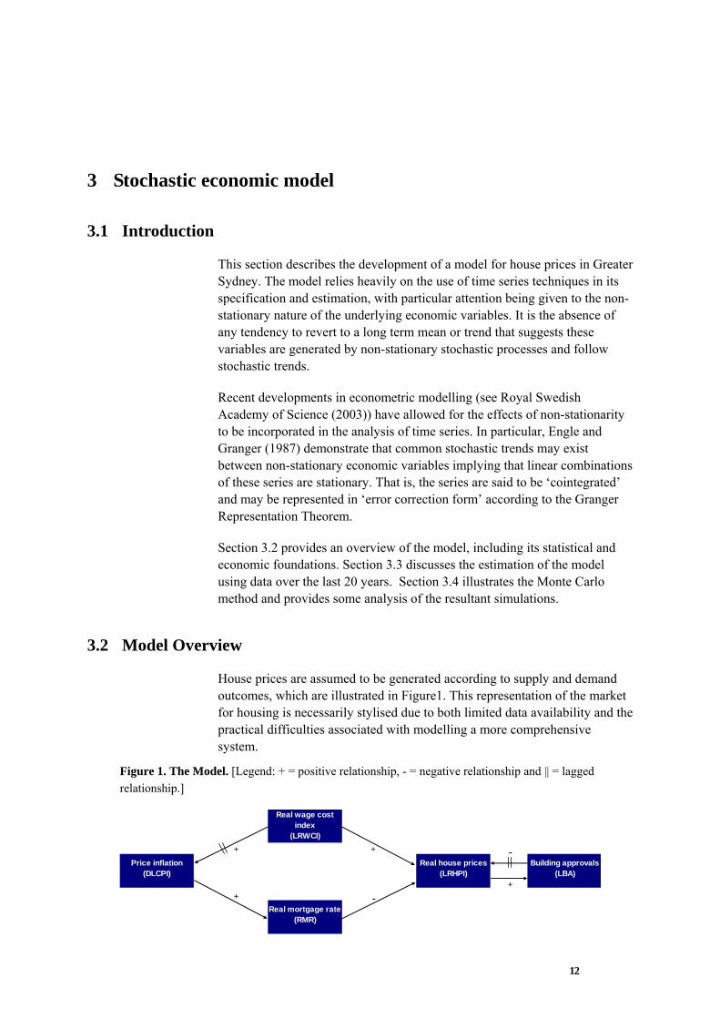
House prices are assumed to be generated according to supply and demand outcomes, which are illustrated in Figure1. This representation of the market for housing is necessarily stylised due to both limited data availability and the practical difficulties associated with modelling a more comprehensive system.

Figure 1. The Model. [Legend: + = positive relationship, - = negative relationship and || = lagged relationship.]

Price inflation(DLCPI)

Real wage cost index

(LRWCI)

Real house prices (LRHPI)

Real mortgage rate (RMR)

Building approvals(LBA)

++

+ +

-

-

13

The supply of housing, to the right of Figure 1, is captured exclusively by the number of building approvals, which is the Reserve Bank of Australia’s (RBA) preferred measure of investment in new dwelling construction. The hypothesised interaction is fairly intuitive: an increase in real house price levels will stimulate new dwelling construction causing a rise in building approvals, which, after a time lag, will result in housing supply growth and with other things being equal, a fall in real prices.

The demand for housing, to the left of Figure 1, is generated via a combination of real wage levels, real mortgage rates and inflation. As the diagram suggests, the interaction of these variables is largely circular in nature. An increase in real wage levels stimulates aggregate demand (including demand for housing), which will place upwards pressure on house prices. If this situation is sustained sufficiently long to outstrip aggregate supply, inflation will rise above the RBA’s target rate, leading to a rise in official interest rates with a knock-on effect to the real mortgage rate. The relationship between real mortgage rates and real house prices will be negative due to the increased cost of borrowing. A more detailed discussion of the determination of house prices may be found in section III.1 of the PricewaterhouseCoopers UK Economic Outlook (October 1999).

A Vector Error Correction Model (VECM) was used to capture these hypothesised economic features. The advantages of a VECM in this context are twofold:

• Long-run equilibrium effects and short-run dynamics are identified explicitly; and

• All economic series are determined simultaneously on the basis of the equilibrium relationship and their own (combined) history;

To identify the long-run equilibrium, the VECM takes advantage of any cointegrating relationships that may exist between the non-stationary economic series (see Section 3.3) used in its estimation. Statistically, these cointegrating relationships represent linear combinations of the (non-stationary) series that are, in fact, stationary as described in Engle and Granger (1987). When appropriately restricted, these linear combinations may be interpreted in terms of hypothesised economic relationships, such as that discussed above (see, for example, Johansen and Juselius (1990)).

14

3.3 Model Estimation

3.3.1 Data

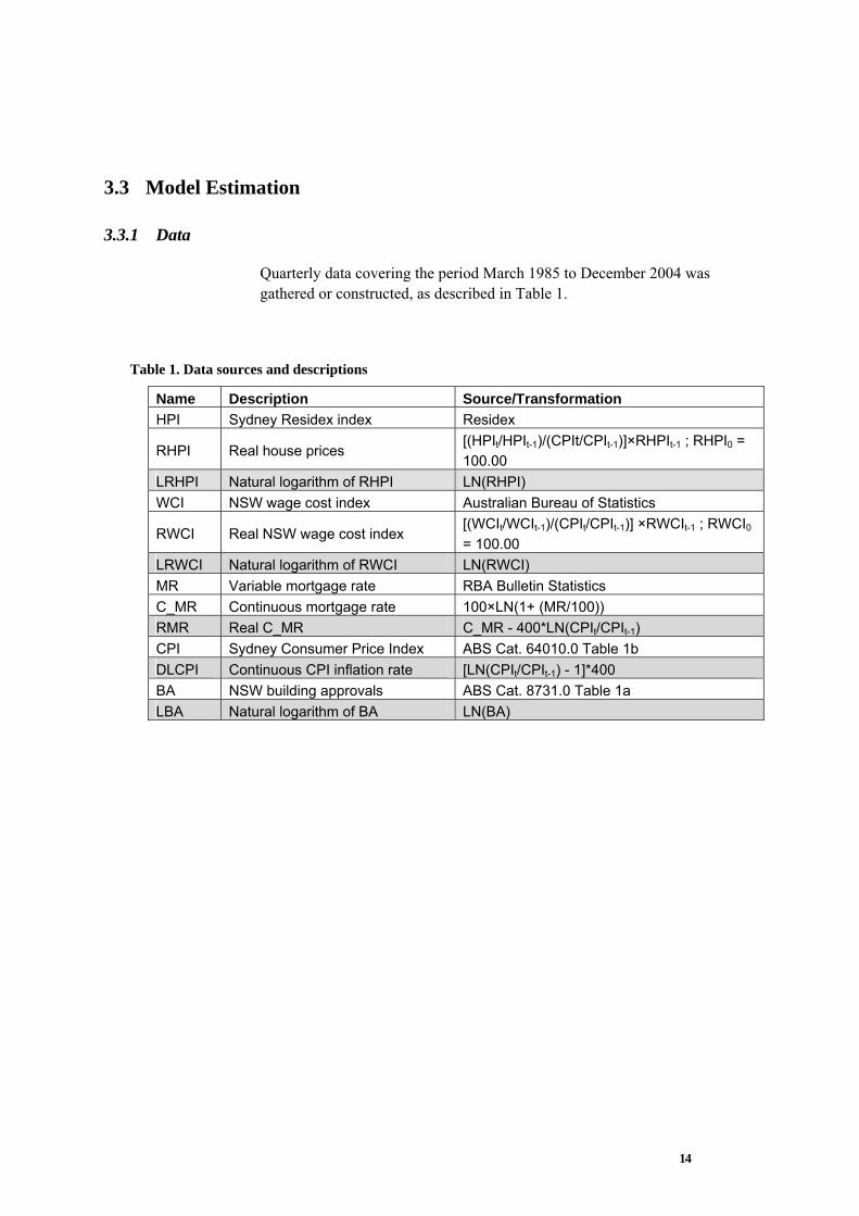
Quarterly data covering the period March 1985 to December 2004 was gathered or constructed, as described in Table 1.

Table 1. Data sources and descriptions

Name Description Source/Transformation HPI Sydney Residex index Residex

RHPI Real house prices [(HPIt/HPIt-1)/(CPIt/CPIt-1)]×RHPIt-1 ; RHPI0 = 100.00

LRHPI Natural logarithm of RHPI LN(RHPI) WCI NSW wage cost index Australian Bureau of Statistics

RWCI Real NSW wage cost index [(WCIt/WCIt-1)/(CPIt/CPIt-1)] ×RWCIt-1 ; RWCI0 = 100.00

LRWCI Natural logarithm of RWCI LN(RWCI) MR Variable mortgage rate RBA Bulletin Statistics C_MR Continuous mortgage rate 100×LN(1+ (MR/100)) RMR Real C_MR C_MR - 400*LN(CPIt/CPIt-1) CPI Sydney Consumer Price Index ABS Cat. 64010.0 Table 1b DLCPI Continuous CPI inflation rate [LN(CPIt/CPIt-1) - 1]*400 BA NSW building approvals ABS Cat. 8731.0 Table 1a LBA Natural logarithm of BA LN(BA)

15

3.3.2 Data Testing

The highlighted series in Table 2 were used for the estimation of the VECM. As discussed in Section 3.2, these series must be non-stationary if a long-run relationship is to be identified. The usual test for non-stationarity is the Augmented Dickey Fuller (1979) (ADF) test with a null hypothesis of non-stationarity. The results are presented in Table 2.

Table 2. Augmented Dickey Fuller testing. A more detailed discussion of this testing is provided in the Appendix.

Series ADF specification Test statistic 95% Critical

value LRHPI Trend; Lag 2 -3.2251 -3.4659LRWCI Trend; Lag 0 -3.1227 -3.4659RMR Intercept; Lag 2 -2.3278 -2.8976DLCPI Intercept; Lag 2 -2.1454 -2.8976LBA Intercept; Lag 0 -3.3963 -2.8976∆LRHPI Intercept; Lag 0 -5.0112 -2.8981∆LRWCI Intercept; Lag 0 -7.3213 -2.8981∆RMR Intercept; Lag 1 -11.7523 -2.8981∆DLCPI Intercept; Lag 0 -10.9587 -2.8981∆LBA Intercept; Lag 0 -9.9348 -2.8981

The ADF regressions (refer Appendices) test for the presence of unit roots causing non-stationarity. If x unit roots are present, the series is said to be integrated of order x, or I(x). Differencing an I(x) series x times will result in stationarity. The VECM requires the series to be I(1), that is, the null should be accepted for the series in levels and rejected for the series in differences. Table 2 shows this to be the case for all series except LBA, which appears to be stationary in levels. However, given that LBA is non-stationary at the 1% level, we consider this series to be appropriate for inclusion in the VECM.

16

3.3.3 Model Specification

The VECM to be fitted to the data is given in Equation 1 below.

tt

p

iititt DXXX εαβµ +Ψ+∆Γ++=∆ ∑

−

=−−

1

11

` (1)

Where, Xt = {LRHPI, LRWCI, RMR, DLCPI, LBA};

t = September 2000 Otherwise

εt is the vector of residuals at time t µ, α, β, Гi, Ψ are parameter matrices

p is the lag order

Points to note include:

• Dt is a dummy variable included to remove the once-off inflationary effects associated with the introduction of the Goods and Services Tax (GST);

• The number of columns (i.e. rank, r) of β determines the number of cointegrating relationships present in the VECM;

• The parameter α can be interpreted as the speed of adjustment to the equilibrium relationship[s] contained in β;

• To ensure consistent and unbiased estimation, it is necessary for the εt’s to possess multivariate normal distributions that are serially independent.

We also note that a VECM represents a restricted Vector Autoregressive (VAR) model of the I(1) model variables in levels. This is an extension (from two dimensions) of the Granger Representation Theorem (see Engle and Granger (1987)).

⎩⎨⎧

=01

tD

17

Lag Order Selection

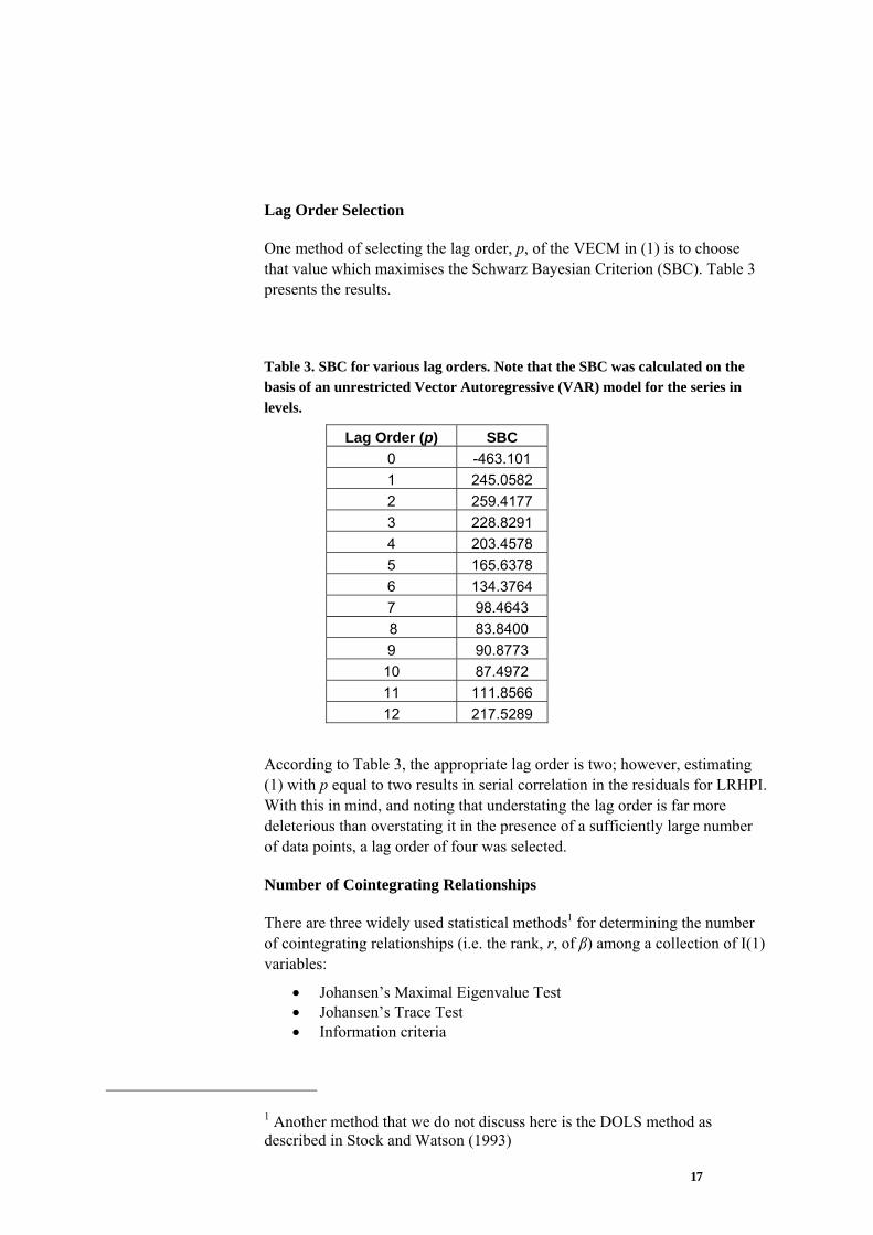
One method of selecting the lag order, p, of the VECM in (1) is to choose that value which maximises the Schwarz Bayesian Criterion (SBC). Table 3 presents the results.

Table 3. SBC for various lag orders. Note that the SBC was calculated on the basis of an unrestricted Vector Autoregressive (VAR) model for the series in levels.

Lag Order (p) SBC 0 -463.101 1 245.0582 2 259.4177 3 228.8291 4 203.4578 5 165.6378 6 134.3764 7 98.4643 8 83.8400 9 90.8773 10 87.4972 11 111.8566 12 217.5289

According to Table 3, the appropriate lag order is two; however, estimating (1) with p equal to two results in serial correlation in the residuals for LRHPI. With this in mind, and noting that understating the lag order is far more deleterious than overstating it in the presence of a sufficiently large number of data points, a lag order of four was selected.

Number of Cointegrating Relationships

There are three widely used statistical methods1 for determining the number of cointegrating relationships (i.e. the rank, r, of β) among a collection of I(1) variables:

• Johansen’s Maximal Eigenvalue Test • Johansen’s Trace Test • Information criteria

1 Another method that we do not discuss here is the DOLS method as described in Stock and Watson (1993)

18

For details of the first two tests we refer the reader to Johansen (1991).

The results for the series LRHPI, LRWCI, RMR, DLCPI and LBA are presented in Table 4.

Table 4. Beta rank testing. LL = Log Likelihood; AIC = Akaike Information Criterion; SBC = Schwarz Bayesian Criterion; HQC = Hannan-Quinn Criterion.

Johansen’s Maximal Eigenvalue Test

Null Alternative Statistic 95% Critical

Value 90%Critical

Value r = 0 r = 1 32.9911 33.64 31.02r<= 1 r = 2 18.9924 27.42 24.99r<= 2 r = 3 16.0845 21.12 19.02r<= 3 r = 4 7.5648 14.88 12.98r<= 4 r = 5 2.3764 8.07 6.50

Johansen’s Trace Test

Null Alternative Statistic 95% Critical

Value 90%Critical

Value r = 0 r>= 1 78.0092 70.49 66.23r<= 1 r>= 2 45.0181 48.88 45.70r<= 2 r>= 3 26.0257 31.54 28.78r<= 3 r>= 4 9.9412 17.86 15.75r<= 4 r = 5 2.3764 8.07 6.50

Information Criteria

Rank Maximized

LL AIC SBC HQC

r = 0 413.4288 328.4288 229.3727 288.8412r = 1 429.9244 335.9244 226.3799 292.1451r = 2 439.4206 338.4206 220.7185 291.3812r = 3 447.4628 341.4628 217.9339 292.0947r = 4 451.2452 342.2452 215.2203 291.4799r = 5 452.4334 342.4334 214.2431 291.2024

At the 95% confidence level, the Trace test suggests a single cointegrating relationship while the Maximal Eigenvalue test supports the null hypothesis of no cointegration. The SBC also supports this null hypothesis, while the AIC and HQC imply five and one cointegrating relationships respectively.

19

In order to reconcile these disparate results, we note that the conclusion of the Maximal Eigenvalue test is marginal; that is, while it suggests no cointegration is present at the 95% confidence level, it supports a single cointegrating vector at the 90% confidence level. In addition, the presence of five cointegrating vectors, as given by the AIC, implies each of the modelled series are stationary, which contradicts the testing carried out in Section 3.3.2.

In light of the above, a beta rank of r = 1 seems appropriate. Moreover, this result is consistent with the discussion in Section 3.2, which alluded to a single long run equilibrium relationship existing between the series.

Residual Testing

A requirement of the maximum likelihood estimation procedure we have adopted (see Johansen (1991)) is that the residuals of (1) are normally distributed and independent (or at least uncorrelated) through time2. Assuming beta takes the form given in the third column of Table 6, the results of tests to this effect are as reported in Table 5.

Table 5. Residual testing. CV = Critical Value. Note the null hypotheses are the absence of serial correlation, the presence of normality, and the absence of heteroskedasticity respectively.

Serial Correlation3 Normality4 Heteroskedasticity5 Statistic p-value Statistic p-value Statistic p-value

LRHPI 3.6034 46.2% 6.6895 3.5% 8.0602 0.5%LRWCI 1.4460 83.6% 0.4323 80.6% 0.5710 45.0%RMR 15.0464 0.5% 9.5052 0.9% 0.0015 96.9%DLCPI 13.6016 0.9% 8.2208 1.6% 0.0063 93.7%LBA 6.2059 18.4% 8.0919 1.7% 0.1815 67.0%

The p-values represent the probability that the relevant test statistic is greater than or equal to its observed value assuming the null hypothesis is true; that is, the p-value can be thought of as the probability that the null hypothesis is true. Therefore, a p-value below a specified significance level will lead to a rejection of the null hypothesis.

2 We note that if the residuals are both normally distributed and serially uncorrelated, they are also serially independent. 3 Godfrey’s Lagrange Multiplier test for autocorrelation 4 Jarque-Bera test for normality 5 Lagrange Multiplier type test based on the regression of squared residuals on squared fitted values

20

At a 1% significance level, the results in Table 5 suggest that:

• The residuals of the equation for RMR are serially correlated and non-normal;

• The residuals of the equation for DLCPI are serially correlated; and

• The variance of the residuals of the equation for LRHPI is dependent on the values of one or more model variables (i.e. exhibits heteroskedasticity).

From a purely statistical point-of-view, the results of the above testing would appear to invalidate the estimation procedure. However, we must bear in mind that alternative specifications of the testing may lead to different, but equally applicable, conclusions. This is especially relevant here as the conclusions we have drawn are marginal at the 1% significance level. In particular,

• The Durbin-Watson test for serial correlation yields insignificant (at the 1% level) results at lags 1 through 12 for both RMR and DLCPI residuals;

• The Anderson-Darling goodness-of-fit test reveals the RMR residuals to be normally distributed; and

• The Engle Lagrange Multiplier test for Autoregressive Conditional Heteroskedasticity (ARCH) effects produces insignificant (at the 1% level) results at lags 1 through12 for the LRHPI residuals.

In light of these results, we conclude that the residuals are multivariate normal white noise.

3.3.4 The long-run equilibrium relationship

Although (1) specifies the error correction equations of each of the five endogenous model variables, we will concentrate our discussion on the error correction equation of LRHPI, which is given by:

(2)

Where, Yt = {LRWCI, RMR, DLCPI, LBA}; µ1, α1, Ψ1, εt

1 = the first elements of µ, α, Ψ and εt in (1) Гi

1 = the first row of Гi in (1) θ = the final four elements of β in (1)

( ) 11

3

1

11111 tt

iitittt DXYLRHPILRHPI εθαµ +Ψ+∆Γ+−+=∆ ∑

=−−−

21

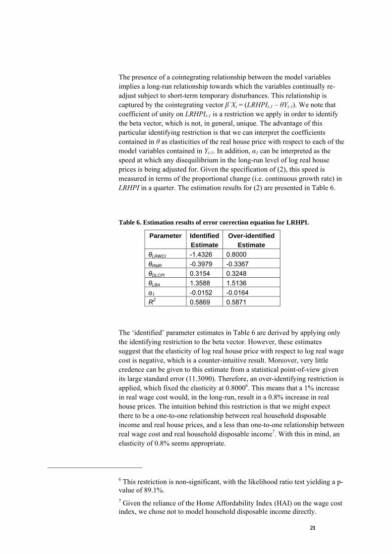
The presence of a cointegrating relationship between the model variables implies a long-run relationship towards which the variables continually re-adjust subject to short-term temporary disturbances. This relationship is captured by the cointegrating vector β`Xt = (LRHPIt-1 – θYt-1). We note that coefficient of unity on LRHPIt-1 is a restriction we apply in order to identify the beta vector, which is not, in general, unique. The advantage of this particular identifying restriction is that we can interpret the coefficients contained in θ as elasticities of the real house price with respect to each of the model variables contained in Yt-1. In addition, α1 can be interpreted as the speed at which any disequilibrium in the long-run level of log real house prices is being adjusted for. Given the specification of (2), this speed is measured in terms of the proportional change (i.e. continuous growth rate) in LRHPI in a quarter. The estimation results for (2) are presented in Table 6.

Table 6. Estimation results of error correction equation for LRHPI.

Parameter IdentifiedEstimate

Over-identified Estimate

θLRWCI -1.4326 0.8000 θRMR -0.3979 -0.3367 θDLCPI 0.3154 0.3248 θLBA 1.3588 1.5136 α1 -0.0152 -0.0164 R2 0.5869 0.5871

The ‘identified’ parameter estimates in Table 6 are derived by applying only the identifying restriction to the beta vector. However, these estimates suggest that the elasticity of log real house price with respect to log real wage cost is negative, which is a counter-intuitive result. Moreover, very little credence can be given to this estimate from a statistical point-of-view given its large standard error (11.3090). Therefore, an over-identifying restriction is applied, which fixed the elasticity at 0.80006. This means that a 1% increase in real wage cost would, in the long-run, result in a 0.8% increase in real house prices. The intuition behind this restriction is that we might expect there to be a one-to-one relationship between real household disposable income and real house prices, and a less than one-to-one relationship between real wage cost and real household disposable income7. With this in mind, an elasticity of 0.8% seems appropriate.

6 This restriction is non-significant, with the likelihood ratio test yielding a p-value of 89.1%. 7 Given the reliance of the Home Affordability Index (HAI) on the wage cost index, we chose not to model household disposable income directly.

22

Conversely, a 1% increase in the level of building approvals is associated with a 1.51% increase in real house prices in the long run. This result is surprising as we originally posited that increased building approvals would eventually lead to a fall in real house prices due to growth in the supply of housing stock (see Figure 1). However, since the cointegrating relationship represents contemporaneous equilibrium levels of each of the model variables and, historically, increased building approvals have been associated with strong growth in real house prices, this conclusion is not entirely unexpected.

The elasticities of real house prices with respect to real mortgage rates and consumer price inflation are, respectively, -33% and 32%8. For example, a 1% increase in real mortgage rates over the course of a quarter will result in a 33% fall in real house prices. Clearly, this is an unrealistic outcome. However, as the nominal mortgage rate historically has been stable compared to the inflation rate, a fall in the real mortgage rate is strongly correlated to a rise in the inflation rate. Therefore, noting the positive inflation rate elasticity of real house prices (i.e. 32%), the long run net effect of a 1% increase in real mortgage rates on real house prices, for example, is likely to be small. Notwithstanding the magnitude of these elasticities, their signs are broadly sensible. That is, an increase in the inflation rate may be viewed by prospective home owners as a sign of expected growth in the inflation rate, therefore encouraging investment in housing as an inflation hedge. This is at odds with the relationship presented in Figure 1, which suggests the inflation rate does not directly impact on house prices in the long run. Conversely, the negative impact of increased real mortgage rates on real house prices is as expected.

Finally, the over-identified estimate of α1 reveals the speed of adjustment to the long run relationship to be relatively slow, with real house price adjustments to equilibrium occurring at a rate of 1.6% per quarter. That is, all things being equal, we would expect house prices to reach equilibrium after approximately 15 years. We can extend this result to incorporate the speed at which the entire system (i.e. not just log real house prices) adjusts to equilibrium by examining the ‘persistence profile’. This profile illustrates how the impact of a system wide shock to the cointegrating vector (i.e. β`Xt) resolves over time. The shock is defined by the covariance matrix of εt in (1), and scaled to equal unity on impact.

8 As we are modelling real mortgage rates and consumer price inflation as percentages, the parameter estimates (θRMR and θDLCPI) are decimals not percentages.

23

Figure 2. Persistence profile of cointegrating vector to system-wide shock

0.0

0.2

0.4

0.6

0.8

1.0

1.2

0 5 10 15 20 25

Therefore, the entire system reaches equilibrium after around 4 years. This is substantially quicker than real house prices alone due to the allowance of interaction effects between all of the model variables in the long-run adjustment process. Nonetheless, this remains a comparatively lengthy ‘equilibrating timeframe’ (see Pesaran and Shin (1996)).

3.3.5 Impulse Response Analysis

The primary limitation of analysing the long-run relationship in isolation is that it fails to capture the complex short-run interactions that occur within the VECM. Therefore, we derive impulse response functions, which show how a model variable of interest responds, over time, to a single standard error shock in another model variable. Again, we will focus our discussion on real house prices. Figure 3 through Figure 6 show the impulse responses of LRHPI to shocks in each of the five model variables as a function of the projection quarter.

Figure 3. Impulse response of LRHPI to a 1 s.e. shock to LRHPI.

0.0%

1.0%

2.0%

3.0%

4.0%

5.0%

6.0%

0 10 20 30 40

24

Figure 4. Impulse response of LRHPI to a 1 s.e. shock to RMR.

-4.0%

-3.5%

-3.0%

-2.5%

-2.0%

-1.5%

-1.0%

-0.5%

0.0%0 10 20 30 40

Figure 5. Impulse response of LRHPI to a 1 s.e. shock to LRWCI.

-3.0%

-2.5%

-2.0%

-1.5%

-1.0%

-0.5%

0.0%0 10 20 30 40

Figure 6. Impulse response of LRHPI to a 1 s.e. shock to LBA.

0.0%

2.0%

4.0%

6.0%

8.0%

10.0%

12.0%

0 10 20 30 40

25

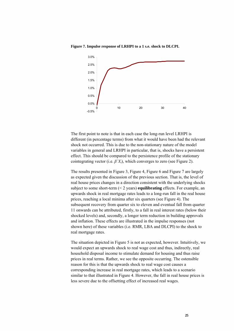
Figure 7. Impulse response of LRHPI to a 1 s.e. shock to DLCPI.

-0.5%

0.0%

0.5%

1.0%

1.5%

2.0%

2.5%

3.0%

0 10 20 30 40

The first point to note is that in each case the long-run level LRHPI is different (in percentage terms) from what it would have been had the relevant shock not occurred. This is due to the non-stationary nature of the model variables in general and LRHPI in particular, that is, shocks have a persistent effect. This should be compared to the persistence profile of the stationary cointegrating vector (i.e. β`Xt), which converges to zero (see Figure 2).

The results presented in Figure 3, Figure 4, Figure 6 and Figure 7 are largely as expected given the discussion of the previous section. That is, the level of real house prices changes in a direction consistent with the underlying shocks subject to some short-term (< 2 years) equilibrating effects. For example, an upwards shock in real mortgage rates leads to a long-run fall in the real house prices, reaching a local minima after six quarters (see Figure 4). The subsequent recovery from quarter six to eleven and eventual fall from quarter 11 onwards can be attributed, firstly, to a fall in real interest rates (below their shocked levels) and, secondly, a longer term reduction in building approvals and inflation. These effects are illustrated in the impulse responses (not shown here) of these variables (i.e. RMR, LBA and DLCPI) to the shock to real mortgage rates.

The situation depicted in Figure 5 is not as expected, however. Intuitively, we would expect an upwards shock to real wage cost and thus, indirectly, real household disposal income to stimulate demand for housing and thus raise prices in real terms. Rather, we see the opposite occurring. The ostensible reason for this is that the upwards shock to real wage cost causes a corresponding increase in real mortgage rates, which leads to a scenario similar to that illustrated in Figure 4. However, the fall in real house prices is less severe due to the offsetting effect of increased real wages.

26

3.4 Simulation

The method of simulation is based on the VECM presented in (1) with some adjustments to reflect recent market conditions9. For each projection quarter (t: t œ {1, 2…n}), m independent random drawings from εt were taken. In accordance with results from the residual testing carried out in Section 3.3.3, was taken to be a set of independent multivariate normal random vectors.

Given that the frequency of claims in the LMI business is most strongly dependent on the growth rate of nominal house prices10, we deal exclusively with these simulations. Figure 8 presents a selection of percentiles and sample simulations of the quarterly nominal growth rate over 40 projection quarters. The most recent historical quarterly growth rates are also provided.

Figure 8. Quarterly growth rates in nominal house prices in Greater Sydney

9 In particular, these adjustments relate to the covariance matrix εt and current expectations of the long-run growth rates of model variables. 10 Nominal house prices were derived by combing the inflation rate and real house price levels, which are both direct outputs of the model.

{ }ntt 1=ε

27

Figure 8 is useful insofar as it offers a means of superficially analysing whether the simulations are plausible realisations of the growth rate. However, it does not offer any insight into whether the model is capable of generating extreme outcomes that are likely to have a significant impact on the claim experience, and therefore solvency, of the LMI business. In particular, the insurer will want to know the probability of realising several consecutive quarters of negative nominal house price growth as well as the average growth rate should this occur.

To this end, Figure 9 presents a histogram providing the empirical probabilities associated with maximum run lengths of negative nominal house prices growth. So, for example, the probability that there will be no more than 2 consecutive quarters of negative house price growth in 40 projection quarters is 20%. Figure 10 presents the average negative growth rate associated with these runs, with each dot representing a single simulation. Therefore, continuing the example, simulations possessing a maximum run length of 2 have mean negative growth rates ranging from -3.9% to -0.05%.

Figure 9. Distribution of maximum run lengths of quarterly negative nominal house price growth

28

Figure 10. Average negative quarterly nominal house price growth rate associated with the maximum run lengths in Figure 9

The above analysis illustrates the model’s potential to generate extreme outcomes in the housing market. For example, in excess of 20 consecutive quarters of negative nominal growth rates with a mean of -3.7% per quarter is possible albeit highly unlikely. Therefore, we can have confidence that the empirical distribution of nominal house price growth adequately captures the inherent uncertainty in the market.

3.5 Conclusions

The above analysis and discussion has demonstrated that house prices in Greater Sydney can be adequately modelled using a VECM. This conclusion is subject to some caveats, however.

• Firstly, in the absence of further testing we can not be sure that a VECM ‘Data Generation Process’ (DGP) is the closest econometric approximation to the true DGP.

• Secondly, the short-term component of the model is heavily over-parameterised, that is, a large proportion of the parameter estimates are statistically insignificant.

• Thirdly, while the model residuals could be classified as multivariate normal white noise at the 1% significance level, not all can be classified as white noise at the 5% significance level. This suggests

29

that some of the parameter estimates may be biased and the model may fail to capture significant non-linear effects.

Therefore, this model, like any other, must be applied with care.

We do however believe that this model is sufficiently robust to be used in assessing economic risk for LMI business and risk margins in general under APRA requirements.

30

4 Stochastic Valuation

4.1 Reserving

4.1.1 Deterministic valuation

In performing the deterministic valuation we have set the relevant projection assumptions equal to the median results from the stochastic economic model.

For all other assumptions we have made a specific deterministic assumption i.e. discharge rate, investment return, claims admin expenses and recoveries. The relevant assumptions feed into the claim frequency and claim size model which we then use to project future claims costs (as per Section 2.4).

This then provides us with the deterministic liability. This is the deterministic estimate from a standard deterministic valuation. However we will need to make a distinction between this and the median (or mean) result from the stochastic valuation. We will discuss this further below.

The methodology we adopt to calculate the deterministic liability estimate is considered to be equivalent to a single simulation, albeit with the simulated economic assumptions set equal to the median results (from the stochastic economic model).

4.1.2 Stochastic valuation

In order to run a stochastic valuation (say with 1,000 trials) we follow an iterative process whereby we simply repeat the deterministic calculation 1,000 times. For each calculation we use the projection assumptions coming from a single simulation from the stochastic economic model.

To recap, the simulated values that we use from the stochastic economic model are, namely:

• Mortgage rates

• Price inflation

• Wage inflation.

• House price movements

Note that the first 3 series are used to construct the HAI series.

When we have completed all our iterations we can then summarise the liability in a number of ways, usually by state, LVR, YOE and YOA.

31

In adopting this approach we are making a number of simplifying assumptions, namely:

• Discount factors are unchanged across all simulations. One would expect that the more significant property price reductions would be occurring along with upwards movements in interest rates. The use of a constant discount factor ignores any possible link. We have noted that there is literature in the area of stochastic discount factors. For the purposes of this paper we have ignored this issue but we have highlighted this as an area for further work.

• That the linear relationships underpinning the GLM will be unchanged under all simulations (including the extreme ones). Some of these relationships may break down in such extreme circumstances. However the intent of this work was the estimation of a premium liability at the 75th percentile and we have not placed significant reliance on the upper percentiles (such as 90th and above).

• Fixed rate of discharge. As we noted earlier, analysis has indicated that the rate of discharge is affected by movements in the property price (along with other factors). Some initial modelling indicates that this will increase the variability in the estimate. However, one has to consider how this will interact with any change in the rate of discharge and how rapid or otherwise the exposure runs off. This is an area for further work.

Sample output

The graph below illustrates the run-off in exposure and projected claims, for all years of advance. This is for the run-off exposure for an illustrative insurer, MortCo as at 30 June 2005.

Discharge Model (Deterministic)

2006

2007

2008

2009

2010

2011

2012

2013

2014

2015

2016

2017

2018

2019

Proj

ecte

d Lo

ans

Expo

sed

('000

)

Proj

ecte

d C

laim

s

Pro jected Loans Exposed ('000) Projected Claims

Comments are as follows:

32

• We note that there is a steady run-off in exposure which is consistent with a fixed rate of discharge.

• We note that there is a slight ‘hump’ in projected claims at the 2007 YOE. This is due to the projected experience for the most recent years of advance. We discuss this further below.

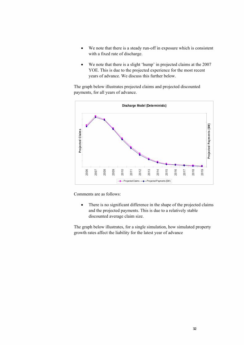
The graph below illustrates projected claims and projected discounted payments, for all years of advance.

Discharge Model (Deterministic)

2006

2007

2008

2009

2010

2011

2012

2013

2014

2015

2016

2017

2018

2019

Proj

ecte

d C

laim

s

Proj

ecte

d Pa

ymen

ts ($

M)

Projected Claims Pro jected Payments ($M )

Comments are as follows:

• There is no significant difference in the shape of the projected claims and the projected payments. This is due to a relatively stable discounted average claim size.

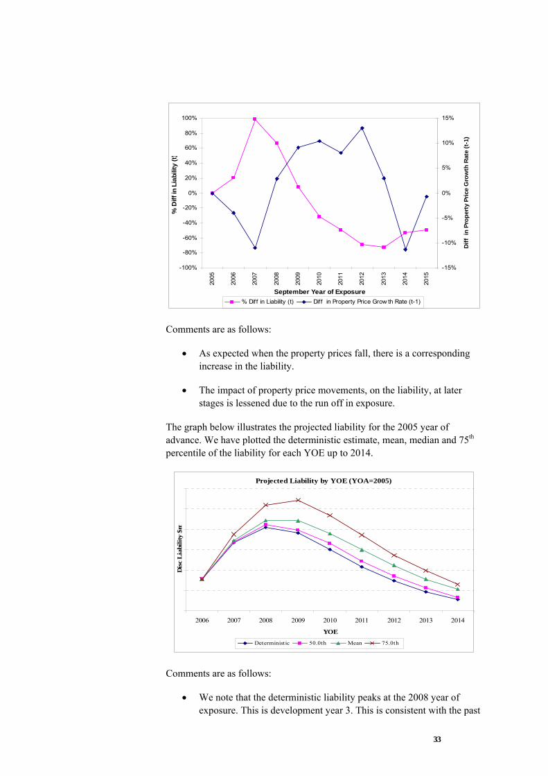
The graph below illustrates, for a single simulation, how simulated property growth rates affect the liability for the latest year of advance

33

-100%

-80%

-60%

-40%

-20%

0%

20%

40%

60%

80%

100%

2005

2006

2007

2008

2009

2010

2011

2012

2013

2014

2015

September Year of Exposure

% D

iff in

Lia

bilit

y (t)

-15%

-10%

-5%

0%

5%

10%

15%

Diff

in

Prop

erty

Pric

e G

row

th R

ate

(t-1

)

% Diff in Liability (t) Diff in Property Price Grow th Rate (t-1)

Comments are as follows:

• As expected when the property prices fall, there is a corresponding increase in the liability.

• The impact of property price movements, on the liability, at later stages is lessened due to the run off in exposure.

The graph below illustrates the projected liability for the 2005 year of advance. We have plotted the deterministic estimate, mean, median and 75th percentile of the liability for each YOE up to 2014.

Projected Liability by YOE (YOA=2005)

2006 2007 2008 2009 2010 2011 2012 2013 2014

YOE

Dis

c L

iabi

lity

$m

Deterministic 50.0th Mean 75.0th

Comments are as follows:

• We note that the deterministic liability peaks at the 2008 year of exposure. This is development year 3. This is consistent with the past

34

claims experience as noted in Section 2.2. We also noted earlier that the GLM formula includes development year as an explanatory variable.

• It is interesting that the shape of the projected liability is largely maintained when we plot the median, mean and 75th percentile. However when we move to the 75th percentile the peak moves to the 2009 year of exposure.

The graph below illustrates the projected liability for the 2003 year of advance using an approach consistent with the preceding graph

Projected Liability by YOE (YOA=2003)

2006 2007 2008 2009 2010 2011 2012 2013 2014

YOE

Dis

c L

iabi

lity

$m

Deterministic 50.0th Mean 75.0th

Comments are as follows:

• This is a similar picture to that in the preceding graph, except we now have 2 more years of development. However in this case the peak occurs at the same YOE for all (including the 75th percentile).

The graph below illustrates the projected liability for all years of advance, again using a consistent approach to the preceding graphs

35

Projected Liability by YOE (all YOA)

2006 2007 2008 2009 2010 2011 2012 2013 2014

YOE

Dis

c L

iabi

lity

$m

Deterministic 50.0th Mean 75.0th

Comments are as follows:

• We note that this consists of a mix of years of advance and has a similar shape to that of the 2005 year of advance. This is not surprising as the recent years of advance (at least for this particular portfolio) make up the vast majority of the liability.

4.2 Stress testing and risk margins

4.2.1 Stress testing

As noted earlier, there are 2 main approaches to stress testing a deterministic valuation, namely sensitivity analysis and scenario analysis.

When we perform a stochastic valuation, sensitivity analysis is no longer appropriate. All feasible assumption values should be captured in the simulations. Any interrelationship between the economic variables and their co-dependence should also be captured by the stochastic economic model.

With a stochastic valuation, possible scenario analysis includes:

• Refitting the economic model over a shorter time period.

• Running the economic model from a different starting point

• Refitting the GLM excluding recent experience

Adopting any of the above scenarios may alter the mean estimate of the stochastic valuation. However this may not significantly alter the relationship between the 75th percentile and the mean and any associated risk margins. This is an area for further work.

36

4.2.2 Risk Margins

The use of a stochastic model allows us to generate results based on a range of outcomes for significant economic variables. This assists in the determination of the major systemic risk factors affecting the liabilities.

The stochastic model shows that many of the outcomes are skewed towards the downside. This is a result of a number of factors:

• The underlying nature of insurance is that the insurer always picks up extreme downside risk, eg. claim numbers can never improve by more than 100% of expected levels, but can deteriorate indefinitely.

• Economic outcomes are themselves skewed to some extent (eg. interest rates can rise more than they can fall).

• Credit risk has threshold effects (eg. the property value on realisation must fall below the outstanding loan amount) which can rapidly accumulate once the conditions are right (eg. a rise in interest rates producing an increase in loan arrears and a fall in property prices).

• Cyclicality in economic outcomes introduces serial correlation in year-to-year outcomes (eg. property price can remain depressed for several years) which have a progressive cumulative effect on insurance outcomes.

• The key relationships are very sensitive to changes in independent variables due to non-linear effects. For example, risk increases exponentially with loan LVR. This introduces further asymmetry in outcomes.

We now discuss the results for the illustrative insurer MortCo.

The modelling showed that the median outcome from the stochastic model lies between 5-10% above that produced from the deterministic model. We suspect this result is dependent on the current benign point in the economic cycle. This means that more of the stochastic economic scenarios increase claim numbers rather than reducing them, thus raising the median outcome relative to that produced by a single scenario (based on the median of the simulated economic variables).

The modelling showed that the mean lies, as expected, above the median. The margin was quite large (in the order of 10-20%), and indicative of a high degree of skewness. This is confirmed when the actual distribution is examined (see below).

37

0

20

40

60

80

100

120

140

160

180

19.892

28.196

36.500

44.804

53.108

61.412

69.716

78.021

86.325

94.629

102.933

111.237

119.541

127.845

136.149

More

ALL

In total the mean (central estimate) of the stochastic model is significantly higher than the deterministic estimate (within the range 15-30%). This raises an interesting issue; that is, when valuing a liability which has significant positive skewness, is a deterministic central estimate truly the mean (i.e. does the valuation model properly allow for the skewness)? This problem is overcome when we use a stochastic model as we can easily calculate the mean of the liability

The 75th percentile result is a further 15-25% above the mean.

The 75th percentile is equivalent to a log-normal coefficient of variation of between 25-35%. However, the CoV-equivalent of the 90th percentile and the 95th percentile were significantly different to that at the 75th percentile. This indicates that the distribution is not log-normal in nature, but more highly-skewed.

Overall risk margins

In order to produce an overall risk margin at the 75th percentile outcome, the results of the stochastic model need to be adjusted for sources of uncertainty other than from future economic factors.

We have allowed for these by adopting coefficients of variation for each of the substantial factors, as follows:

• Data errors and limitations

• Exposure – i.e. projected exposure across various key risk factors

• Model fit error and future process uncertainty

38

Each of these effects is taken to be log-normally distributed, and to be independent from the others, and from systemic economic risk.

These other sources of uncertainty only added a minimal amount to the total CoV. The vast majority of uncertainty, for LMI business, arises from systemic economic risk.

For this particular portfolio, the 75th percentile produced a risk margin below the APRA minimum (of half of the overall CoV).

Therefore the provision will include a risk margin based on half the COV.

4.3 Conclusion

The above analysis and discussion has demonstrated a number of key points which we summarise below:

• A stochastic valuation model can be used to determine the central estimate and the risk margin. This ensures a consistent approach.

• The stochastic approach will more accurately capture the inherent skewness (non-lognormal) in the liability for this class of business.

• The use of lognormal assumption may not be appropriate and may lead to misleading results

• A deterministic approach to valuing this insurance liability may not appropriately capture the skewness and the deterministic estimate may thus be significantly different from the true mean of the liability.

• Systemic economic risk accounts for the vast majority of uncertainty for this class of business

39

5 Further work

The preceding analysis and discussion highlighted a number of areas for further work. We summarise these areas below:

• Discount factors are unchanged across all simulations. One would expect that the more significant property price reductions would be occurring along with upwards movements in interest rates. Deterministic discount factors, as used here, ignore any possible link and should be replaced with stochastic discount factors

• Stochastic discharge factors. As we noted earlier, analysis has indicated that the rate of discharge is affected by movements in the property price (along with other factors). Some initial modelling indicates that this will increase the variability in the estimate. However, one has to consider how this will interact with any change in the rate of discharge and how rapid or otherwise the exposure runs off.

• Default model: We have modelled the numbers of claims with respect to loans exposed. Before a claim occurs there are a number of preceding stages including the loan falling into arrears and any subsequent default. Given a reasonable volume of data we would develop a probability of default (PD) model and then a loss given default model (LGD) using, for example, Markov chain techniques.

• Loan characteristic model dynamics. Another unknown is the behavioural aspect of borrowers (and subsequent repayments and/or default/claims). Certain borrowers may be more likely to churn than others and preliminary analysis has identified certain predictors of this behaviour. This is an area for further work.

• Asset – liability modelling: The use of a stochastic economic model to estimate the liability can be extended to simulate returns on the assets and thus assist the insurer in assessing capital requirements.

40

6 Acknowledgements and references

Acknowledgements:

We are indebted to Conor O’Dowd, Sylvia Wong and Ajay Singh for the contribution they have made to the evolution of this paper through discussion, debate and challenge. While acknowledging the great benefit we have obtained from this dialogue, any errors or omissions are entirely those of the authors alone.

We would also like to acknowledge St George Insurance Pte Ltd and in particular Mr Peter Morgan and the credit risk team for their assistance in this project.

References:

• Abelson, P., R. Joyuex, G. Milunovich and D. Chung (2004), “House prices in Australia: 1970 to 2003 facts and explanations”, Macquarie Economics Research Papers

• Ayat, L. and P. Burridge (2000), “Unit root tests in the presence of uncertainty about the non-stochastic trend”, Journal of Econometrics, 95(1), 71-96

• Chen, M. and K. Patel (1998), “House price dynamics and granger causality: an analysis of Taipei new dwelling market”, Journal of the Asian Real Estate Society, 1(1), 101-126

• Dickey, D. and W. Fuller (1979), “Distribution of the estimators for autoregressive time series with a unit root”, Journal of the American Statistical Association, 74, 427-431

• Engle, R.F. and C.W.J Granger, 1987, “Co-integration and error correction: Representation, estimation and testing”, Econometrica, 55, 251-276

• Garratt, A., Lee, K., Pesaran, M. H. and Shin, Y. (2001), “A Long Run Structural Macroeconometric Model of the UK”, The Economic Journal , 113(487), 412-455

• Johansen, S. (1991), ”Estimation and hypothesis testing of cointegrating vectors in Gaussian vector autoregressive models”, Econometrics, 59, 1551-80

• Johansen, S. and K. Juselius (1990), “Maximum likelihood estimation and inference on cointegration – with applications to the

41

demand for money”, Oxford Bulletin of Economics and Statistics, 52(2)

• Ley S., O’Dowd C., (1997), “The changing face of home lending”, Proceedings of the 11th General Insurance Seminar, November 1997.

• PricewaterhouseCoopers UK Economic Outlook (October 1999)

• Sherris, M., Tedesco, L. and Zehnwirth, B. (1997), “Stochastic Investment Models: Unit Roots, Cointegration, State Space and GARCH Models for Australian data”, ARCH, 1997.1, 95-144.

• Taylor G., (1991a), “Modelling mortgage insurance claims experience: A Case Study”, A Coopers and Lybrand research report

• Taylor G., (1991b), “Economic and Statistical Aspects of Mortgage Insurance Claims Experience”, A Coopers and Lybrand research report

• Taylor G., (1993), “The incidence of risk under credit insurance”, A Coopers and Lybrand research report

• Taylor G., (1994), “Modelling mortgage insurance claims experience: A Case Study”, ASTIN Bulletin , 24(1) 1994

• Royal Swedish Academy of Science Advanced information on the Bank of Sweden Prize in Economic Sciences in Memory of Alfred Nobel, 8. October, 2003. “Time Series Econometrics: Cointegration and Autoregressive Conditional Heteroscedasticity (Nobel Laureates in Economics, 2003, Robert F. Engle and Clive W. J. Granger)”

42

Appendices

A. Augmented Dickey Fuller Testing

The Augmented Dickey Fuller regression tests for the presence of random walk effects – and thus a unit root causing non-stationarity – by performing the following regressions on the univariate series Xt:

∑

∑

∑

=−−

=−−

=−−

+∆+++=∆

+∆++=∆

+∆+=∆

q

ittitt

q

ittitt

q

ittitt

ZaXtZ

ZaXZ

ZaXZ

11110

1110

111

δργγ

δργ

δρ

Where,

δt = IID(0,σ2)

ρ, γ0, γ1, and the ai’s are constants to be estimated

(Note that the autoregressive terms contained in the summation operator are designed to remove serial correlation from the εt’s.)

Depending on the values of γ0 and γ1, the null hypothesis is that the series is a random walk, a random walk with drift, or a random walk with a linear trend. In each case the null is equivalent to ρ = 0, which is tested for using the t ratio applied to special critical values.

In order to select the appropriate form of the ADF regression (i.e. nature of deterministic component and lag length, q), we apply the following testing strategy adapted from Ayat and Burridge (2000).

Step 1

Perform preliminary unit root testing invariant to a linear trend under the null; i.e. test for ρ = 0 under the third specification in (A.1), where the lag length q is selected according to the minimum Schwarz Bayesian Information Criteria (SBC) in conjunction with Durbin’s t test for first order autocorrelation of residuals.

(A.1)

43

Step 2a

If the unit root is not rejected at Step 1, then provisionally maintain the null hypothesis (ρ = 0) and estimate:

t

q

iitit ZZ ec

10 +∆+=∆ ∑

=−β (A.2)

Then test for the null that γ 1 = 0 in (A.1) using the t ratio on β0 referred to standard tables.

Step 2b

If the unit root is rejected at Step 1, then test for γ 1 = 0 using the t ratio on γ 1 – based on an estimation of the third specification in (A.1) – referred to standard tables.

Step 3a

If γ 1 = 0 is rejected at Step 2, then stop. (The unit root test carried out in Step 1 contains the ‘correct’ deterministic component.)

Step 3b

If γ 1 = 0 is not rejected at Step 2, perform a provisional unit root test invariant to the mean under the null; i.e. test for ρ = 0 under the second specification in (A.1), where the lag length q is again selected according to the minimum SBC in conjunction with Durbin’s t test.

Step 4a

If a unit root is rejected at Step 3b, then stop.

Step 4b

If the unit root is not rejected at Step 3b, test the magnitude of the initial observation, Z0, relative to the increments in Z using the following test ratio referred to N(0,1):

( )∑ ∆=

− 210

tZT

Zz (A.3)

Where, T = number of observations.

Step 5a

44

If z differs significantly from 0 in Step 4b, then stop.

Step 5b

If the null of z = 0 is accepted in Step 4b, then perform a unit root test that is not invariant to the mean under the null; i.e. test for ρ = 0 under the first specification in (1), where the lag length q is again selected according to the minimum SBC in conjunction with Durbin’s t test.